From images to descriptors and back again Patrick Pérez

funding:

FGMIA 2014

Searching in image and video databases

One scenario: query-by-example

Input: one query image

Output

Ranked list of “relevant” visual content

Information on object/scene visible in query

Some existing systems

Google Image and Goggles / Amazon Flow / Kooaba (Qualcom)

2

Visual search

1/16/2014

Raw images can’t be compared pixel-wise

Relevant information is lost in clutter and changes place

No invariance or robustness

Meaningful and robust representation

Global statistics

Local descriptors aggregated in a global signature

Efficient approximate comparisons

3

Large scale image comparison

1/16/2014

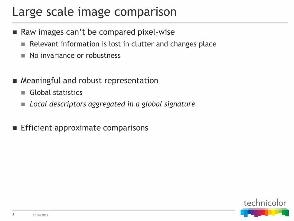
Select/detect image fragments, normalize and describe them

Robust to some geometric and photometric changes

Most popular: SIFT ∈ ℝ128

Precise image comparison: match fragments based on descriptors

Works very well … but way too expensive on a large scale

Local descriptors

4

[Mikolajczyk , Schmid. IJCV 2004]

[Lowe. IJCV 2004]

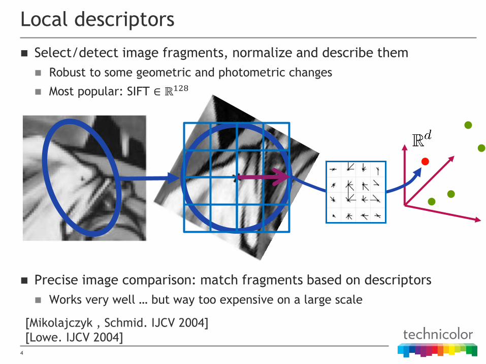
Forget about precise descriptors

Vector-quantization using a dictionary of

𝑘 “visual words” learned off-line

Forget about fragment location

Counting visual words

BoW: sparse fixed size signature by

aggregation of a variable number of

quantized local descriptors

5

Bag of “Visual Words” pipeline

1/16/2014

extract local descriptors quantization

BoW visual word histogram

query image

[Sivic, Zisserman. ICCV 2003][Csurca et al. 2004]

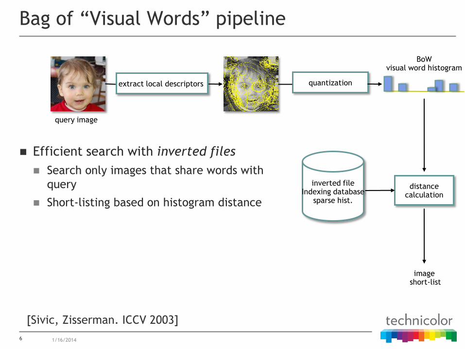
Efficient search with inverted files

Search only images that share words with

query

Short-listing based on histogram distance

6

Bag of “Visual Words” pipeline

1/16/2014

extract local descriptors quantization

distance calculation

image short-list

query image

inverted file Indexing database

sparse hist.

[Sivic, Zisserman. ICCV 2003]

BoW visual word histogram

Geometrical post-verification

Match local features

Infer most likely geometric transform

Rank short list based on goodness-of-fit

7

Bag of “Visual Words” pipeline

1/16/2014

extract local descriptors quantization

distance calculation

image short-list

query image

geometrical post-verification

inverted file Indexing database

sparse hist.

final image short-list

[Sivic, Zisserman. ICCV 2003]

BoW visual word histogram

Precise search requires large dictionary (𝑘 ~20,000-200,000 words)

Difficult to learn

Costly to compute (𝑘 distances per descriptor) on database

Memory footprint still too large (~10KB per image)

With 40GB RAM, search 10M images in 2s

Does not scale up to web-scale (∝ 1011 images)

Contribution*

Novel aggregation of local descriptors into image signature

Combined with efficient indexing

Low memory footprint (20B per image, 200MB RAM for 10M images)

Fast search (50ms to search within 10M images on laptop)

8

Limitations and contributions

1/16/2014

*[Jégou, Douze, Schmid, Pérez. CVPR 2010]

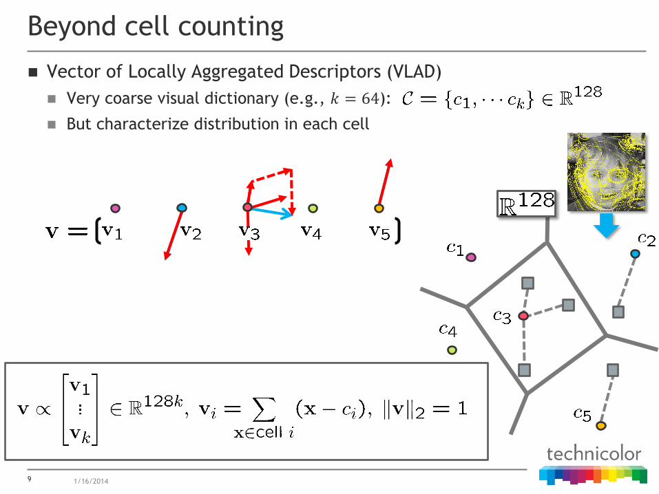
Vector of Locally Aggregated Descriptors (VLAD)

Very coarse visual dictionary (e.g., 𝑘 = 64):

But characterize distribution in each cell

9

Beyond cell counting

1/16/2014

Vectors of size 𝐷 = 128 × 𝑘, 𝑘 SIFT-like blocks

10 1/16/2014

VLAD

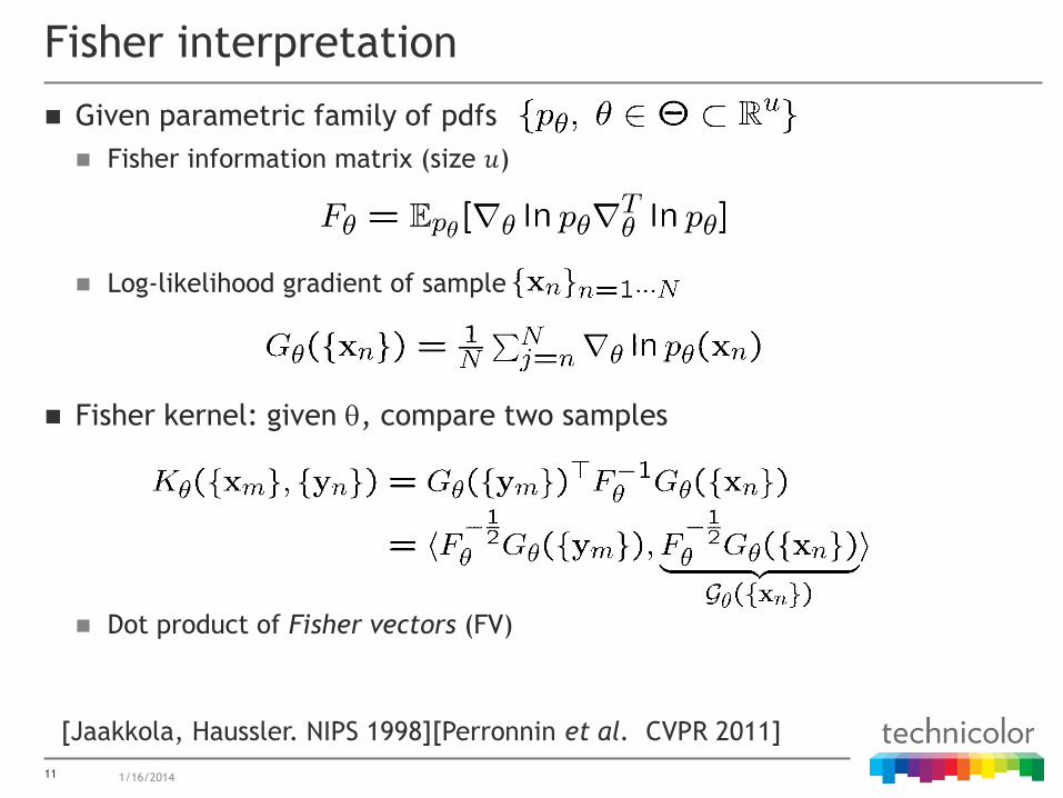
Given parametric family of pdfs

Fisher information matrix (size 𝑢)

Log-likelihood gradient of sample

Fisher kernel: given , compare two samples

Dot product of Fisher vectors (FV)

11

Fisher interpretation

1/16/2014

[Jaakkola, Haussler. NIPS 1998][Perronnin et al. CVPR 2011]

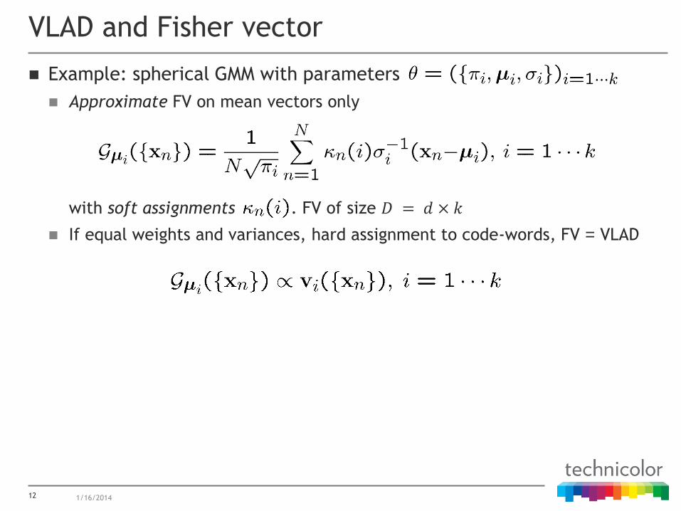
Example: spherical GMM with parameters

Approximate FV on mean vectors only

with soft assignments . FV of size 𝐷 = 𝑑 × 𝑘

If equal weights and variances, hard assignment to code-words, FV = VLAD

12

VLAD and Fisher vector

1/16/2014

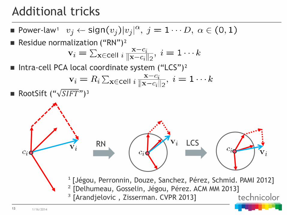
Power-law¹

Residue normalization (“RN”)²

Intra-cell PCA local coordinate system (“LCS”)²

RootSift (“ 𝑆𝐼𝐹𝑇”)³

13

Additional tricks

1/16/2014

¹ [Jégou, Perronnin, Douze, Sanchez, Pérez, Schmid. PAMI 2012]

² [Delhumeau, Gosselin, Jégou, Pérez. ACM MM 2013]

³ [Arandjelovic , Zisserman. CVPR 2013]

RN LCS

Comparisons to BoW on Holidays (1500 images with relevance GT)

14

Exhaustive search

1/16/2014

Image signature dim mAP (%)

BoW-20K 20,000 43.7

BoW-200K 200,000 54.0

VLAD-64 8192 51.8

+ 𝛼 = 0.2 54.9

+ 𝑆𝐼𝐹𝑇 57.3

+ RN 63.1

+ LCS 65.8

+ dense SIFTs 76.6

Towards large scale search

PCA reduction of image signature to 𝐷’ = 128

Very fine quantization with Product Quantizer (PQ)*

Results on Oxford105K and Holydays+1M Flickr distractors

15

Getting short and compact

1/16/2014

Image signature Ox105K Hol+1M

Best VLAD-64 (8192 dim) 45.6 −

Reduced (128 dim) 26.6 39.2

Quantized (16 bytes) 22.2 32.3

*[Jégou, Douze, Schmid. PAMI 2010]

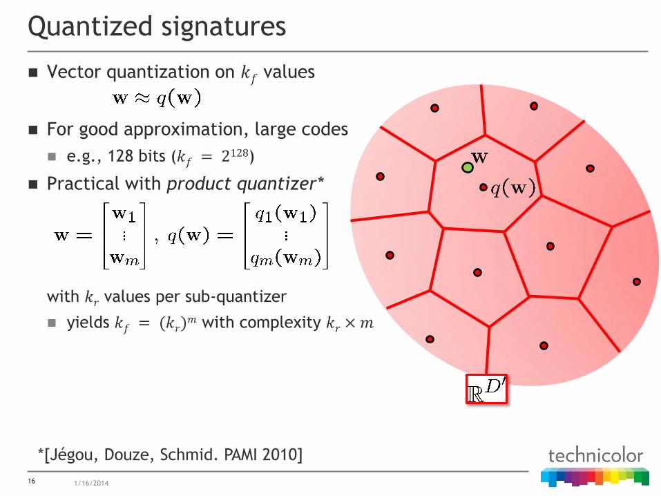
Vector quantization on 𝑘𝑓 values

For good approximation, large codes

e.g., 128 bits (𝑘𝑓 = 2128)

Practical with product quantizer*

with 𝑘𝑟 values per sub-quantizer

yields 𝑘𝑓 = (𝑘𝑟)𝑚 with complexity 𝑘𝑟 × 𝑚

16

Quantized signatures

1/16/2014

*[Jégou, Douze, Schmid. PAMI 2010]

17

Quantized signatures

1/16/2014

8 components

256 quantized values

1 Byte 16 Bytes index ⇐

Given query signature v, distance

to a basis signature w:

Exhaustive search among 𝑁𝑏 basis

images

18

Asymmetric Distance Computation (ADC)

1/16/2014

𝑘𝑟 possible values

𝑚𝑘𝑟 distances + (𝑚 − 1)𝑁𝑏 sums

Two-level quantization of signatures

Coarse quantization (e.g., 𝑘𝑐 = 28 values)

One inverted list per code-vector

Compare only within lists of 𝑤 nearest code-vectors to query

Fine PQ quantization of residual signatures (e.g., 𝑘𝑓 = 2128)

Search among 𝑁𝑏 basis images

𝑤 = 16, 𝑚 = 16, 𝑘𝑟 = 𝑘𝑐 = 256 ⇒ one sum only per image with almost no

accuracy change!

19

ADC with Inverted Files (IVF-ADC)

1/16/2014

𝑚𝑘𝑟 distances + 𝑤 𝑚 − 1 𝑁𝑏𝑘𝑐−1 sums

20

Performance w.r.t. memory footprint

1/16/2014

Image signature bytes mAP

(%)

BoW-20K 10,364 43.7

BoW-200K 12,886 54.0

FV-64 59.5

Spectral Hashing* 128 bits 16 39.4

PQ, 𝑚 = 16, 𝑘𝑟 = 256 16 50.6

bytes

*[Weiss et al. NIPS 2008]

21

Large scale experiments

1/16/2014

Holidays + up to 10M distractors from Flickr

𝑘 = 64, exact, 7s

𝑘 = 256, 320B

𝑘 = 64, 16B, 45ms

BoW-200K

Copydays + up to 100M distractors from Exalead

22

Larger scale experiments

1/16/2014

64B, 245ms

64B, 160ms

[GIST: Oliva, Torralab. PBR 2006][GISTIS: Douze et al. AMC-MM 2009]

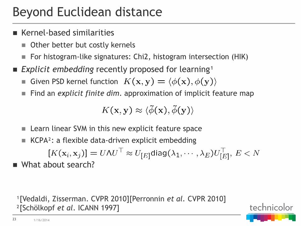
Kernel-based similarities

Other better but costly kernels

For histogram-like signatures: Chi2, histogram intersection (HIK)

Explicit embedding recently proposed for learning¹

Given PSD kernel function

Find an explicit finite dim. approximation of implicit feature map

Learn linear SVM in this new explicit feature space

KCPA²: a flexible data-driven explicit embedding

What about search?

23

Beyond Euclidean distance

1/16/2014

¹[Vedaldi, Zisserman. CVPR 2010][Perronnin et al. CVPR 2010]

²[Schölkopf et al. ICANN 1997]

Simple proposed approach* (“KPCA+PQ”)

Embed database vectors with learned KPCA

Efficient Euclidean ANN with PQ coding

Kernel-based re-ranking in original space

Competitors: binary search in implicit space

Kernelised Locally Sensitive Hashing (KLSH) [Kulis, Grauman. ICCV09]

Random Maximum Margin Hashing (RMMH) [Joly, Buisson. CVPR11]

Experiments

Data: 1.2M images from ImageNet with BoW signatures

Chi2 similarity measure

Tested also: “KPCA+LSH”(binary search in explicit space)

24

Approximate search with short codes

1/16/2014

*[Bourrier, Perronnin, Gribonval, Pérez, Jégou. TR 2012]

Results averaged over 10 runs

25 1/16/2014

Recall@R

𝐸 = 128, 𝐵 = 256 bits, 𝑀 = 1024

Recall@1000

𝐵 = 32 → 256bits

Reconstructing an image from descriptors

26 1/16/2014

If sparse local descriptors only are known

Better insight into what local descriptors capture, with multiple

applications

extract key points and local descriptors

original image

“Invert” the process ?

Reconstructing an image from descriptors

27 1/16/2014

Possible to some extent

[Weinzaepfel, Jégou, Pérez. CVPR’2011]

Inverting local description

28 1/16/2014

Local description, severely lossy by construction

Color, absolute intensity, spatial arrangement in each cell are lost

Non-invertible many-to-one map

Example-based regularization: use key-points from arbitrary images

Patch collection must be large and diverse enough (e.g., 6M)

…

Inverting local description

29 1/16/2014

Progressive collage

Dead-leaf procedure, largest patches first

Seamless cloning*

Harmonic correction: smooth change to remove boundary discrepancies

Final hole filling

Harmonic interpolation

Assembling recovered patches

30 1/16/2014

*[Pérez, Gangnet, Blake. Siggraph 2003]

Reconstruction

31 1/16/2014

Reconstruction

32 1/16/2014

Reconstruction

1/16/2014 33

New: reconstruction from dense local features

Human-understandable images can be reconstructed

Visual insight into information exploited by detectors and classifiers

Visual information leakage in image indexing systems: privacy?

34

Outlook

1/16/2014

¹ [D'Angelo, Alahi, P. Vandergheynst. ICPR 2012]

² [Vondrick, Khosla, Malisiewicz, Torralba. ICCV 2013]

local binary pattern¹

HOG (Hoggles)²