Embed Size (px)
Citation preview
From homogenization to averaging in cellular flows
Gautam Iyer∗ Tomasz Komorowski† Alexei Novikov‡ Lenya Ryzhik§
August 1, 2011
Abstract
We consider an elliptic eigenvalue problem with a fast cellular flow of amplitude A, in a two-dimensional domain with L2 cells. For fixed A, and L→∞, the problem homogenizes, and hasbeen well studied. Also well studied is the limit when L is fixed, and A → ∞. In this case thesolution equilibrates along stream lines.
In this paper, we show that if both A → ∞ and L → ∞, then a transition between thehomogenization and averaging regimes occurs at A ≈ L4. When A L4, the principal Dirichleteigenvalue is approximately constant. On the other hand, when A L4, the principal eigenvaluebehaves like σ(A)/L2, where σ(A) ≈
√AI is the effective diffusion matrix. A similar transition
is observed for the solution of the exit time problem. The proof in the homogenization regimeinvolves bounds on the second correctors. Miraculously, if the slow profile is quadratic, theseestimates can be obtained using drift independent Lp → L∞ estimates for elliptic equations withan incompressible drift. This provides effective sub and super-solutions for our problem.
1 Introduction
Consider an advection diffusion equation of the form
∂tϕ+Av(x) · ∇ϕ−∆ϕ = 0. (1.1)
where A is the non-dimensional strength of a prescribed vector field v(x). Under reasonable as-sumptions when A→∞, the solution ϕ becomes constant on the trajectories of v. Indeed, dividing(1.1) by A and passing to the limit A→∞ formally shows
v(x) · ∇ϕ = 0,
which, of course, forces ϕ to be constant along trajectories of v. Well known “averaging” results [8,15,20] study the slow evolution of ϕ(t, x) across various trajectories.
On the other hand, if we fix A = 1, classical homogenization results [2,12,20] determine the longtime behavior of solutions of (1.1). For such results it is usually convenient to choose ε 1 small,and rescale (1.1) to time scales of order 1/ε2, and distance scales of order 1/ε. This gives
∂tϕε +1
εv(xε
)· ∇ϕε −∆ϕε = 0. (1.2)
∗Department of Mathematical Sciences, Carnegie Mellon University, Pittsburgh, PA 15213; [email protected]†Institute of Mathematics, UMCS, pl. Marii Curie-Sk lodowskiej 1, 20-031, Lublin and IMPAN, ul. Sniadeckich 8,
00-956 Warsaw, Poland, e-mail: [email protected]‡Department of Mathematics, Pennsylvania State University, State College PA 16802, [email protected]§Department of Mathematics, Stanford University, Stanford, CA 94305, USA, e-mail: [email protected]
1
Assuming v is periodic, and that the initial condition varies slowly (i.e. ϕε(x, 0) is independent ofε), standard homogenization results show that ϕε → ϕ, as ε → 0. Further, ϕ is the solution of theeffective problem
∂ϕ
∂t= ∇ · (σ∇ϕ), (1.3)
and σ is the effective diffusion matrix, which can be computed as follows. Define the correctors χ1,. . . , χn to be the mean-zero periodic solutions of
−∆χj + v(x) · ∇χj = −vj(x), j = 1, . . . , n. (1.4)
Then
σij = δij +1
|Q|
∫Q∇χi · ∇χj dx, i, j = 1, . . . , n. (1.5)
Q is the period cell of the flow v(x), and δij is the Kronecker delta function.The main focus of this paper is to study a transition between the two well known regimes
described above. To this end, rescale (1.1) by choosing time scales of the order 1/ε2 and lengthscales of order 1/ε. This gives
∂tϕε,A +A
εv(xε
)· ∇ϕε,A −∆ϕε,A = 0, (1.6)
where A 1 and ε 1 are two independent parameters. Of course, if we keep ε fixed, and sendA → ∞, the well known averaging results apply. Alternately, if we keep A fixed and send ε → 0,we are in the regime of standard homogenization results. The present paper considers (1.6) withboth ε→ 0 and A→∞. Our main result shows that if v is a 2D cellular flow, then we see a sharptransition between the homogenization and averaging regimes at A ≈ 1/ε4.
Before stating our precise results (Theorems 1.1 and 1.2 below), we provide a brief explanation asto why one expects the transition to occur at A ≈ 1/ε4. For simplicity and concreteness, we choosethe stream function H(x1, x2) = 1
π sin(πx1) sin(πx2), and define v(x1, x2) = (−∂2H, ∂1H). Even inthis simple setting, to the best of our knowledge, the transition from averaging to homogenizationhas not been studied before.
First, for any fixed A, we let σ(A) = (σij(A)) denote the effective diffusion matrix obtained inthe limit ε→ 0 (see [18] for a comprehensive review). If χAj is the mean zero, 2-periodic solution to
−∆χAj +Av(x) · ∇χj = −Avj(x), for j ∈ 1, 2, (1.7)
then the effective diffusivity (as a function of A) is given by (1.5). As A → ∞, the behaviour ofthe correctors χAj is well understood [5, 6, 10,17,19,21,24,25]. Except on a boundary layer of order
1/√A, each of the functions χj(x) + xj become constant in cell interiors. Using this one can show
(see for instance [5, 6]) that asymptotically, as A→∞, the effective diffusion matrix behaves like
σ(A) = σ0
√AI + o(
√A) (1.8)
Here I is the identity matrix, and σ0 > 0 is an explicitly computable constant. Consequently, if weconsider (1.6), with the Dirichlet boundary conditions on the unit square, we expect
ϕε,A(x, t) ≈ exp(−σ0
√At), as t→∞, for small ε. (1.9)
On the other hand, if we keep ε fixed and send A→∞, we know [8,25] that ϕ becomes constanton stream lines of H. In particular, because of the Dirichlet boundary condition on the outside
2
boundary, we must also have ϕ = 0 on the boundary of all interior cells. Since these cells have sidelength ε, we expect
ϕε,A(x, t) ≈ exp(−π2t/ε2), as t→∞ for large A. (1.10)
Matching (1.9) and (1.10) leads us to believe√A ≈ 1/ε2 marks the transition between the two
regimes.
With this explanation, we state our main results. Our first two results study the averagingto homogenization transition for the principal Dirichlet eigenvalue. Let L be an even integer,D = [−L/2, L/2] × [−L/2, L/2] be a square of side length L, and A > 0 be given. We studythe principal eigenvalue problem on D
−∆ϕ+Av · ∇ϕ = λϕ in D
ϕ = 0 on ∂D
ϕ > 0 in D,
(1.11)
as both L,A→∞. We observe two distinct behaviors of λ with a sharp transition. If A L4, thenthe principal eigenvalue stays bounded, and can be read off using the variational principle in [3] inthe limit A→∞. This is the averaging regime, and exactly explains (1.10). On the other hand, ifA L4, then the principal eigenvalue is of the order σ(A)/L2. This is the homogenization regime,and when rescaled to a domain of size 1, exactly explains (1.9). Our precise results are stated below.
Theorem 1.1 (The averaging regime). Let ϕ = ϕL,A be the solution of (1.11) and λ = λL,A be theprincipal eigenvalue. If A→∞, and L = L(A) varies such that
lim infA→∞
√A
L2 logA logL> 0, (1.12)
then there exist two constants λ0, λ1, independent of L and A, such that
0 < λ0 6 λL,A 6 λ1 <∞ (1.13)
for all A sufficiently large.
Theorem 1.2 (The homogenization regime). As with Theorem 1.1, let ϕ = ϕL,A be the solutionof (1.11) and λ = λL,A be the principal eigenvalue. If L→∞, and A = A(L) varies such that
1
cL4−α 6 A 6 cL4−α, for some α > 0, (1.14)
then there exists a constant C = C(α, c) > 0, independent of L and A, such that
1
C
√A
L26 λL,A 6 C
√A
L2(1.15)
for all L sufficiently large.
Remark. In the special case where A = Lβ, for β > 4, assumption (1.12) is satisfied, and consequentlythe principal eigenvalue remains bounded and non-zero. For β < 4, assumption (1.14) is satisfiedand the principal eigenvalue behaves like that of the homogenized equation.
3
In the averaging regime (Theorem 1.1), the proof of the upper bound in (1.13) follows directlyusing ideas of [3]. The lower bound, however, is much more intricate. The main idea is to controlthe oscillation of ϕ between neighbouring cells, and use this to show that the effect of the coldboundary propagates inward along separatrices, all the way to the center cell. The techniques usedare similar to [7, 16]. The main new (and non-trivial) difficulty in our situation is that the numberof cells also increases with the amplitude. This requires us to estimate the oscillation of ϕ betweencells in terms of energies localised to each cell (Proposition 2.4, below). Here the assumption thatL is not too large comes into play. Finally, the key idea in the proof is to use a min-max argument(Lemma 2.5, below) to show that ϕ is small on the boundaries of all cells.
Moreover, once smallness on separatrices is established, our proof may be modified to show thatunder a stronger assumption
lim infA→∞
√A
L2 logA logL= +∞, (1.16)
we have a precise asymptotics
limA→∞
λL,A = inf
∫Q|∇w|2
∣∣∣∣ w ∈ H10 (Q),
∫Qw2 = 1, and w · ∇v = 0
, (1.17)
where Q is a single cell. This is the same as the variational principle in [3]. We remark howeverthat [3] only gives (1.17) for fixed L as A→∞.
Turning to the homogenization regime (Theorem 1.2), we remark first that homogenization ofeigenvalues has not been as extensively studied as other homogenization problems. This is possiblybecause eigenvalues involve the infinite time horizon. We refer to [1,13,14,22,23] that all study self-adjoint problems for some results on the homogenization of the eigenvalues in oscillatory periodicmedia. The extra difficulties in the present paper come both from two sources. First, since theproblem is not self adjoint, a variational principle for the eigenvalue is not available. Second, as Aand L tend to ∞, we don’t have suitable aprori bounds because either the domain is not compact,or the effective diffusivity is unbounded.
Our proof uses a multi-scale expansion to construct appropriate sub and super solutions. WhenA is fixed, it usually suffices to consider a multi-scale expansion to the first corrector. However, inour situation, this is not enough, and we are forced to consider a multi-scale expansion up to thesecond corrector.
Of course an asymptotic profile, and explicit bounds are readily available [6] for the first corrector.However, to the best of our knowledge, bounds on the second corrector as A → ∞ have not beenstudied. There are two main problems to obtaining these bounds. The first problem is appearanceof that terms involving the slow gradient of the second corrector multiplied by A. In general, wehave no way of bounding these terms. Luckily, if we choose our slow profile to be quadratic, thenthese terms idnetically vanish and present no problem at all!
The second problem with obtaining bounds on the second corrector is that it satisfies an equationwhere the first order terms depend on A. So one would expect the bounds to also depend on A,which would be catastrophic in our situation. However, for elliptic equations with a divergence freedrift, we have apriori Lp → L∞ estimates which are independent of the drift [4, 7]. This, combinedwith an explicit knowledge of the first corrector, allows us to obtain bounds on the second correctorthat decay when A L4.
The sub and super solutions we construct for eigenvalue problem are done through the expectedexit time. Since these are interesting in their own right, we describe them below. Let τ = τL,A be
4
the solution of −∆τ +Av · ∇τ = 1 in D
τ = 0 on ∂D,(1.18)
where v and D are as in (1.11). Though we do not use any probabilistic arguments in this paper, itis useful to point out the connection between τ and diffusions. Let X be the diffusion
dXt = −Av(Xt) dt+√
2dWt (1.19)
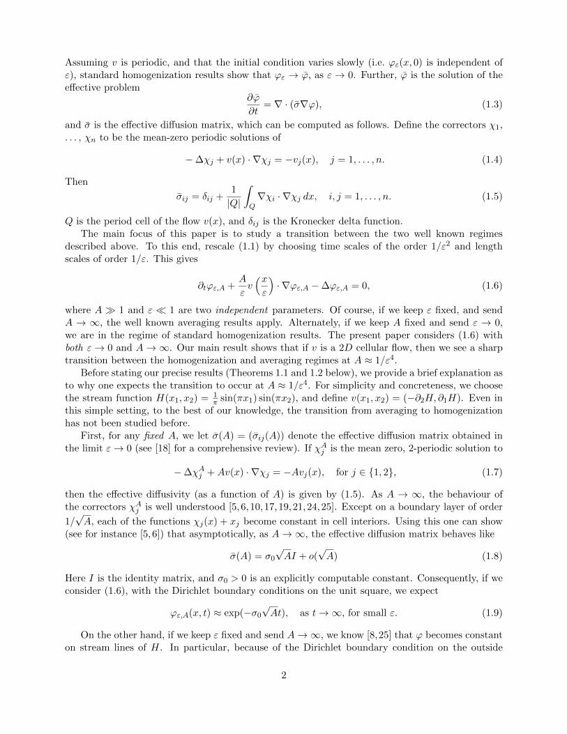
where W is a standard 2-dimensional Brownian motion. It is well known that τ is the expected exittime of the diffusion X from the domain D. Numerical simulations of three realizations of X areshown in Figure 1. Note that for “small” amplitude (A = L3), trajectories of X behave similarly tothose of the Brownian motion. For a “large” amplitude (A = L4.5), trajectories of X tend to moveballistically along the skeleton of the separatrices.
(a) Small amplitude (A = L3) (b) Large amplitude (A = L4.5)
Figure 1: Trajectories of three realizations of the diffusion (1.19).
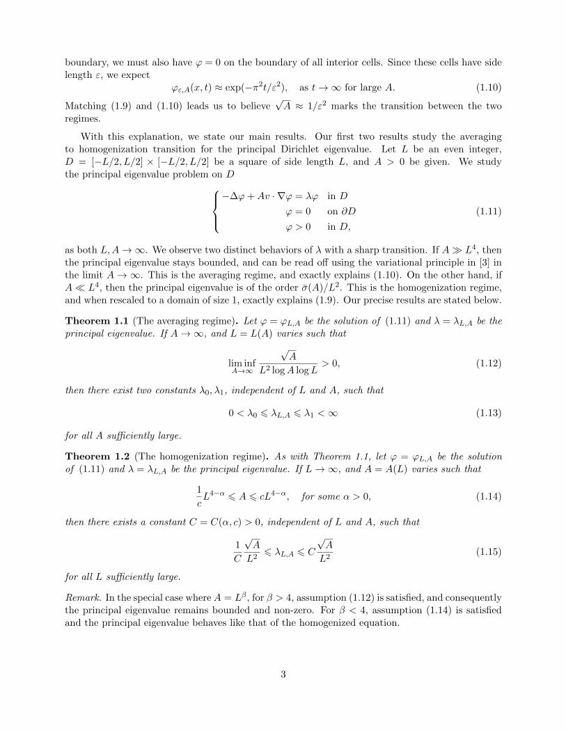
(a) Small amplitude (A = L3) (b) Large amplitude (A = L5)
Figure 2: A contour plot of τ(x, y).
Similar to the eigenvalue problem, the behaviour of τ is described by two distinct regimes witha sharp transition. If A L4, then the stirring is strong enough to force the diffusion X to exit
5
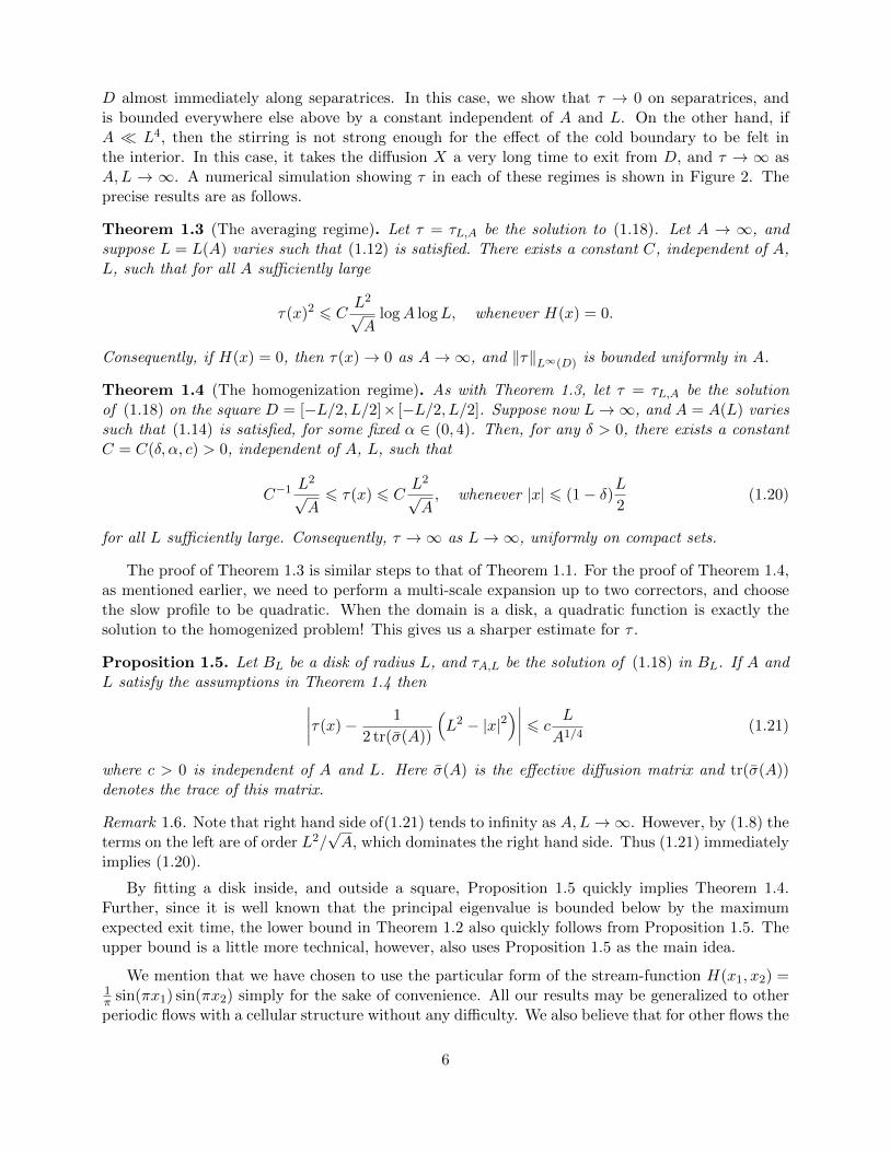
D almost immediately along separatrices. In this case, we show that τ → 0 on separatrices, andis bounded everywhere else above by a constant independent of A and L. On the other hand, ifA L4, then the stirring is not strong enough for the effect of the cold boundary to be felt inthe interior. In this case, it takes the diffusion X a very long time to exit from D, and τ → ∞ asA,L → ∞. A numerical simulation showing τ in each of these regimes is shown in Figure 2. Theprecise results are as follows.
Theorem 1.3 (The averaging regime). Let τ = τL,A be the solution to (1.18). Let A → ∞, andsuppose L = L(A) varies such that (1.12) is satisfied. There exists a constant C, independent of A,L, such that for all A sufficiently large
τ(x)2 6 CL2
√A
logA logL, whenever H(x) = 0.
Consequently, if H(x) = 0, then τ(x)→ 0 as A→∞, and ‖τ‖L∞(D) is bounded uniformly in A.
Theorem 1.4 (The homogenization regime). As with Theorem 1.3, let τ = τL,A be the solutionof (1.18) on the square D = [−L/2, L/2]× [−L/2, L/2]. Suppose now L→∞, and A = A(L) variessuch that (1.14) is satisfied, for some fixed α ∈ (0, 4). Then, for any δ > 0, there exists a constantC = C(δ, α, c) > 0, independent of A, L, such that
C−1 L2
√A
6 τ(x) 6 CL2
√A, whenever |x| 6 (1− δ)L
2(1.20)
for all L sufficiently large. Consequently, τ →∞ as L→∞, uniformly on compact sets.
The proof of Theorem 1.3 is similar steps to that of Theorem 1.1. For the proof of Theorem 1.4,as mentioned earlier, we need to perform a multi-scale expansion up to two correctors, and choosethe slow profile to be quadratic. When the domain is a disk, a quadratic function is exactly thesolution to the homogenized problem! This gives us a sharper estimate for τ .
Proposition 1.5. Let BL be a disk of radius L, and τA,L be the solution of (1.18) in BL. If A andL satisfy the assumptions in Theorem 1.4 then∣∣∣∣τ(x)− 1
2 tr(σ(A))
(L2 − |x|2
)∣∣∣∣ 6 cL
A1/4(1.21)
where c > 0 is independent of A and L. Here σ(A) is the effective diffusion matrix and tr(σ(A))denotes the trace of this matrix.
Remark 1.6. Note that right hand side of(1.21) tends to infinity as A,L→∞. However, by (1.8) theterms on the left are of order L2/
√A, which dominates the right hand side. Thus (1.21) immediately
implies (1.20).
By fitting a disk inside, and outside a square, Proposition 1.5 quickly implies Theorem 1.4.Further, since it is well known that the principal eigenvalue is bounded below by the maximumexpected exit time, the lower bound in Theorem 1.2 also quickly follows from Proposition 1.5. Theupper bound is a little more technical, however, also uses Proposition 1.5 as the main idea.
We mention that we have chosen to use the particular form of the stream-function H(x1, x2) =1π sin(πx1) sin(πx2) simply for the sake of convenience. All our results may be generalized to otherperiodic flows with a cellular structure without any difficulty. We also believe that for other flows the
6
transition from the averaging to the homogenization regime happens when the effective diffusivityσ(A) balances with the domain size L. That is, when the “homogenized eigenvalue” σ(A)/L2 is ofthe same order as the “strong flow” eigenvalue:
limA→∞
σ(A)
L2λL,A≈ 1. (1.22)
We leave this question for a future study.This paper is organized as follows. The averaging regime is considered in Sections 2 and 3. The
former contains the proof of Theorem 1.1 and the latter of Theorem 1.3. The rest of the paperaddresses the homogenization regime. The key step here is Proposition 1.5 proved in Section 4.From this, Theorem 1.4 quickly follows, and the proof is presented the same section. Theorem 1.2is proved in Section 5.
Acknowledgement
GI was supported by NSF grant DMS-1007914, TK by Polish Ministry of Science and HigherEducation grant NN 201419139, AN by NSF grant DMS-0908011, and LR by NSF grant DMS-0908507, and NSSEFF fellowship. We thank Po-Shen Loh for suggesting the proof of Lemma 2.5.
2 The eigenvalue in the strong flow regime
In this section we present the proof of Theorem 1.1. First, we discuss the proof of the upperbound in (1.13), followed by the proof of the corresponding lower bound, and, finally, of the limitingbehavior in (1.17).
2.1 The upper bound
The upper bound for λ in (1.13) follows directly from the techniques of [3]. We carry outthe details below. Following [3], given any test function w ∈ H1
0 (D), and a number α > 0, wemultiply (1.11) by w2/(ϕ+ α) and integrate over D to obtain
λ
∫D
w2ϕ
ϕ+ α= −
∫D
w2∆ϕ
ϕ+ α+A
∫D
w2
ϕ+ αv · ∇ϕ. (2.1)
For the first term on the right, we have
−∫D
w2∆ϕ
ϕ+ α=
∫D∇ϕ ·
(2w(ϕ+ α)∇w − w2∇ϕ
(ϕ+ α)2
)=
∫D|∇w|2 −
∫D
|w∇ϕ− (ϕ+ α)∇w|2
(ϕ+ α)26∫D|∇w|2.
For the second term on the right of (2.1) we have, since u is incompressible,∫D
w2
ϕ+ αv · ∇ϕ =
∫Dw2v · ∇ ln(ϕ+ α) = −2
∫D
ln(ϕ+ α)w(v · ∇w).
Hence, equation (2.1) reduces to
λ
∫D
w2ϕ
ϕ+ α6∫D|∇w|2 − 2A
∫D
ln(ϕ+ α)w(v · ∇w). (2.2)
7
Now, choose w to be any H10 (D) first integral of v (that is, v · ∇w = 0). Then, equation (2.2)
reduces to
λ
∫D
w2ϕ
ϕ+ α6∫D|∇w|2.
Upon sending α→ 0, the Monotone Convergence Theorem shows
λ
∫Dw2 6
∫D|∇w|2
for any H10 (D) first integral of v. Choosing w = H(x), which, of course, does not depend on L, we
immediately see that
λ 6
(∫DH2
)−1 ∫D|∇H|2 =
(L2
∫Q0
H2
)−1
L2
∫Q0
|∇H|2 =
(∫Q0
H2
)−1 ∫Q0
|∇H|2,
where Q0 is any cell in D. This gives a finite upper bound for λ that is independent of L and A.
2.2 The lower bound
The outline of the proof is as follows. The basic idea is that if the domain size L is not toolarge, and the flow is sufficiently strong, the eigenfunction ϕ should be small not only near theboundary ∂D but also on the whole skeleton of separatrices inside D. Therefore, the Dirichleteigenvalue problem for the whole domain D is essentially equivalent to a one-cell Dirichlet problem,which gives the correct asymptotics for the eigenvalue for A large. To this end, we first estimate theoscillation of ϕ along a streamline of v inside one cell that is sufficiently close to the separatrix, andshow that this oscillation is small: see Lemma 2.2. Next, we show that the difference of the valuesof ϕ on two streamlines of v (sufficiently close to the separatrix) in two neighbouring cells must besmall, as in Lemma 2.3 below. These two steps are very similar to those in [7], and their proofs areonly sketched.
Now, considering the ‘worst case scenario’ of the above oscillation estimates, we obtain a point-wise upper bound on ϕ on streamlines of v near separatrices in terms of the principal eigenvalueλ, and ‖ϕ‖2L2 : see Lemma 2.5. Next, we show that the streamlines above enclose a large enoughregion to encompass most of the mass of ϕ2. Finally, we use the drift independent apriori estimatesin [4, 11] to obtain the desired lower bound on λ.
A streamline oscillation estimate
The basic reason behind the fact that the eigenfunction is constant on streamlines is the followingestimate, originally due to S. Heinze [10].
Lemma 2.1. There exists a constant C > 0 so that we have∫D|v · ∇ϕ|2dx 6
C
A
∫D|∇ϕ|2dx =
Cλ
A‖ϕ‖2L2 . (2.3)
Proof. Let us use the normalization ‖ϕ‖L2 = 1. We multiply (1.11) by v · ∇ϕ, and integrate overQi. This gives
A
∫D|v · ∇ϕ|2 = λ
∫Dϕ(v · ∇ϕ) +
∫D
∆ϕ(v · ∇ϕ).
Notice that ∫Dϕ(v · ∇ϕ) =
1
2
∫Dv · ∇
(ϕ2)
= 0,
8
since v · ν = 0 on ∂Qi and ∇ · v = 0. Similarly, we have, as v · ∇ϕ = 0 on ∂D:
∫D
∆ϕ(v · ∇ϕ) = −2∑j=1
∫D∂jϕ (∂jv · ∇ϕ)−
2∑j=1
∫D∂jϕ (v · ∇∂jϕ) +
∫∂D
(ν · ∇ϕ)(v · ∇ϕ) dS
6 ‖∇v‖L∞(Qi)‖∇ϕ‖2L2(D) −
1
2
2∑j=1
∫D∇ ·(v (∂jϕ)2
)= Cλ,
and consequently we obtain (2.3).
The next lemma bounds locally the oscillation on streamlines in terms of the L2-norm of v ·∇ϕ.
Lemma 2.2. Let Qi be any cell. For any δ0 > 0, there exists Γi ⊂ Qi such that Γi is a level set ofH, |H(Γi)| ∈ (δ0, 2δ0), and
supx1,x2∈Γi
|ϕ(x1)− ϕ(x2)|2 6 C1
δ0log
(1
δ0
)∫Qi
|v · ∇ϕ|2. (2.4)
for some constant C independent of A,L, δ0.
We will see that δ0 is the ‘width’ of the boundary layer, and will eventually be chosen to beδ0 ≈ 1/
√A.
Proof. The proof is straightforward and similar bounds have already appeared in [7,16]. We sketchthe details here for convenience. First we introduce curvilinear coordinates in the cell Qi. For this,let (xi, yi) be the center of Qi, and Θi be the solution of
∇Θi · ∇H = 0 in Qi − (xi + t, yi)∣∣ t > 0
Θi(x, y) = tan−1
(y − yix− xi
)on ∂Qi.
(2.5)
As usual, we extend Θ to Qi by defining it to be 0 (or 2π) on (xi + t, yi) | t > 0.In the coordinates (h, θ) given by the functions H and Θi, it is easy to check that
∂ϕ
∂θ=
v · ∇ϕ|∇Θi||∇H|
.
Assume, for simplicity, that H > 0 on Qi. Then for any h ∈ (δ0, 2δ0), we have
supθ1,θ2
|ϕ(h, θ1)− ϕ(h, θ2)|2 6
(∫H=h
|v · ∇ϕ| dθ
|∇Θi||∇H|
)2
6∫H=h
|v · ∇ϕ|2 dθ
|∇Θi||∇H|
∫H=h
dθ
|∇Θi||∇H|
6 C ln
(1
δ0
)∫H=h
|v · ∇ϕ|2 dθ
|∇Θi||∇H|.
The last inequality follows from the fact that∫H=h
dθ
|∇Θi||∇H|6 C ln
1
δ0,
9
as the length element along the contour dl = dθ/|∇Θ|. Now integrating over (δ0, 2δ0), we get∫ 2δ0
δ0
supθ1,θ2
|ϕ(h, θ1)− ϕ(h, θ2)|2 dh 6 C ln1
δ0
∫Qi
|v · ∇ϕ|2
and (2.4) follows from the mean value theorem.
Variation between neighboring cells
Now, we consider two streamlines on which the solution is nearly constant and estimate thepossible jump in the value of ϕ between them.
Lemma 2.3. Let Qi and Qj be two neighbouring cells, Γi ⊂ Qi, Γj ⊂ Qj the respective level setsfrom Lemma 2.2, and let hi = H(Γi), hj = H(Γj). Then there exists xi ∈ Γi and xj ∈ Γj such that
|ϕ(xi)− ϕ(xj)|2 6 Cδ0
∫Qi∪Qj
|∇ϕ|2 + C1
δ0log
(1
δ0
)∫Qi∪Qj
|v · ∇ϕ|2. (2.6)
Proof. Assume again for simplicity that H > 0 on Qi, and Qi is to the left of Qj . Then, using thelocal curvilinear coordinates (h, θ) around the common boundary between the cells Qi and Qj , asin (2.5), we have
ϕ(hi, θ)− ϕ(hj , θ) =
∫ hi
hj
∂ϕ
∂hdh.
Now, let δ1 ∈ (0, π2 ) be fixed. In the region |h| 6 hi, and |θ| 6 δ1, we know that |∇H| ≈ 1 and|∇Θ| ≈ 1. Hence, we have∫
Qi
|∇ϕ|2 > C
∫ δ1
−δ1
∫ hj
hi
∣∣∣∣∂ϕ∂h∣∣∣∣2 >
C
δ0inf|θ|6δ1
|ϕ(hj , θ)− ϕ(hi, θ)|2.
However, Lemma 2.2 shows that
sup|θ|6δ1
|ϕ(hj , θ)− ϕ(hi, θ)|2 6 inf|θ|6δ1
|ϕ(hj , θ)− ϕ(hi, θ)|2 + C1
δ0log
(1
δ0
)∫Qi∪Qj
|v · ∇ϕ|2. (2.7)
This concludes the proof of (2.6).
Variation between two far away cells
For each cell Qi, we set
αi =
∫Qi
(|∇ϕ|2 +A|v · ∇ϕ|2
)dx.
Choosing δ0 = 1/√A, Lemmas 2.2 and 2.3 immediately give the following oscillation estimate.
Proposition 2.4. If Qi and Qj are any two cells, and Γi ⊂ Qi, Γj ⊂ Qj the respective level setsfrom Lemma 2.2, then ∣∣∣∣ sup
xi∈Γi
ϕ(xi)− infxj∈Γj
ϕ(xj)
∣∣∣∣ 6 C(logA)1/2
A1/4
∑line
√αk.
where the sum is taken over any path of cells that connects Qi and Qj, consisting of only horizontaland vertical line segments.
10
Lemma 2.1 implies that ∑j
αj 6 Cλ‖ϕ‖2L2(D), (2.8)
with the summation taken over all cells in D. Now, the key to the proof of the lower bound inTheorem 1.1 is to obtain an estimate on ‖ϕ‖L∞(Γi)
in terms of (∑
i αi)1/2. A direct application of
Cauchy-Schwartz to Proposition 2.4 is wasteful and does not yield a good enough estimate. Whatis required is a more careful estimate of the ‘worst case scenario’ for the values of αi. This is thecontent of our next Lemma.
Lemma 2.5. On any cell Qi, we have
supx∈Γi
|ϕ(x)|2 6 ClogA logL
A1/2
∑all cells
αi 6 ClogA logL
A1/2λ‖ϕ‖2L2(D)
where Γi ⊂ Qi is the level set from Lemma 2.2.
Proof. For notational convenience, in this proof only, we will assume that D = (−L− 12 , L+ 1
2)2 isthe square of side length 2L+1 centered (0, 0), and Qi,j = (x, y) | x ∈ [i− 1
2 , i+12), y ∈ [j− 1
2 , j+ 12)
is the cell with center (i, j). Note that in the present proof we label the cells, (and contours Γijinside the cell Qij we use below) by two indices that correspond to the coordinates of the center ofthe cell.
Let Gi0,j0 denote the set of all paths of cells that join the boundary ∂D to the cell Qi0,j0 using
only horizontal and vertical line segments. Let β = (βi,j) ∈ R(2L+1)2 , βi,j > 0, be a collection ofnon-negative numbers assigned to each cell, and denote
qi0,j0(β) = ming∈Gi0,j0
∑(i,j)∈g
√βi,j . (2.9)
We first claim there exists an explicitly computable constant C, independent of L, β, i0, j0 such that
qi0,j0(β)2 6 C logLL∑
i,j=−Lβi,j , (2.10)
which is an obvious improvement over the Cauchy-Schwartz estimate applied blindly to (2.9). Thisimprovement comes because we are taking the minimum over all such paths in (2.9).
To prove (2.10), we define
qavgi0,j0
(β,G′i0,j0) =1
|G′(i0,j0)|∑
g∈G′i0,j0
∑(i,j)∈g
√βi,j .
where G′(i0,j0) is any collection of (possibly repeated) paths in G(i0,j0). Since the minimum of acollection of numbers is not bigger than the average of any subset, we certainly have
qi0,j0(β) 6 qavgi0,j0
(β,G′i0,j0)
for any collection G′i0,j0 . The idea is to choose such a sub-collection in a convenient way.We prove the claim for (i0, j0) = (0, 0). We choose G′0,0 to consist of (L + 1)! paths, with the
following property. All paths stay in the upper-right quadrant. The last cell visited by all paths is(0, 0). The second to last cell visited by (L+ 1)!/2 paths (half of the collection) is (1, 0), and the
11
second to last cell visited by the remaining paths is (0, 1). Amongst the paths who’s second to lastcell is (1, 0), we choose G′0,0 so that two thirds of these paths have (2, 0) as the third to last cell,and one third have (1, 1) as the third to last cell. Symmetrically, we choose G′0,0 so that amongstall the paths who’s second to last cell is (0, 1), two thirds of these paths have (0, 2) as the third lastcell, and one third have (1, 1) as the third to last cell. Consequently exactly (L+ 1)!/3 paths havethird to last cell (2, 0), exactly (L+ 1)!/3 paths in G′0,0 have third to last cell (1, 1), and exactly(L+ 1)!/3 paths in G′0,0 have third to last cell (0, 2).
Continuing similarly, we see that G′0,0 can be chosen so that for any cell (i, j) with i + j 6 L,
exactly (L+ 1)!/(i+ j + 1) paths visit the cell (i, j) as the (i + j + 1)th to last cell. Finally, weassume that all paths in G′0,0 start on the top boundary and proceed directly vertically downwarduntil they hit a cell of the form (k, L− k).
Let us count how many times each term√βi,j appears in the averaged sum qavg
0,0 (β,G′0,0). Clearly,
if i+j 6 L, then the cell (i, j) appears in exactly (L+1)!i+j+1 paths in G′0,0. On the other hand, if i+j > L,
then the cell (i, j) appears exactly (L+1)!L+1 paths. Consequently, we have
qavg0,0 (β,G′0,0) =
L−1∑k=0
1
k + 1
k∑i=0
√βi,k−i +
1
L+ 1
L∑i=0
L∑j=L−i
√βi,j . (2.11)
We now maximize the sum in (2.11) with the constraint
L∑i,j=0
βij = σ. (2.12)
Let S denote the right side of (2.11), then at the maximizer of S we have
∂S
∂βij=
1
2(L+ 1)√βij
, for i+ j > L,
and∂S
∂βij=
1
2(i+ j + 1)√βij
, for i+ j 6 L.
The Euler-Lagrange equations now imply that
βij =γ
4(L+ 1)2for i+ j > L,
andβij =
γ
4(i+ j + 1)2for 0 6 i+ j 6 L.
Here γ is the Lagrange multiplier that can be computed from the constraint (2.12):
γ(L+ 1)(L+ 2)
4(L+ 1)2+ γ
L−1∑j=0
(j + 1)
4(j + 1)2= σ.
It follows thatγ = σγ(L),
12
with γ(L) = O(1/ logL) as L→ +∞. Hence, for the maximizer we get
S 6C√σ√
logL
L−1∑k=0
1
k + 1+ C√γ = C
√σ logL,
and thus (2.10) holds for i0, j0 = (0, 0). However, it is immediate to see that the previous argumentcan be applied to any cell considering appropriate collection of paths that say up and to the rightof (i0, j0), whence (2.10) holds for all (i0, j0).
With (2.10) in hand, we observe that Proposition 2.4 implies
‖ϕ‖2L∞(Γi0,j0 ) 6 ClogA√Aqi0,j0(α)2 6 C
logA√A
logLL∑
i=−L
L∑j=−L
αi,j 6 ClogA logL√
Aλ‖ϕ‖2L2 ,
where the last inequality follows from Lemma 2.1. This concludes the proof.
Our next step shows that the mass of ϕ2 in the regions enclosed by the level sets Γi is comparableto ‖ϕ‖2L2(D).
Lemma 2.6. Let Qi be a cell, and Γi ⊂ Qi the level set from Lemma 2.2. Let hi = H(Γi), andSi = Qi ∩ |H| < |hi| be a neighbourhood of ∂Qi. Let Q′i = Qi − Si. Then, for A sufficiently large,we have ∑
i
‖ϕ‖2L2(Q′i)>
1
2‖ϕ‖2L2(D) (2.13)
Proof. For any cell Qi, the Sobolev restriction theorem shows∫H=h|ϕ(h, θ)|2 dθ
|∇Θ|= ‖ϕ‖2L2(H−1(h)∩Qi) 6 C‖ϕ‖2H1(Qi)
= C(αi + ‖ϕ‖2L2(Qi)
).
Thus, using curvilinear coordinates with respect to the cell Qi, and assuming, for simplicity, thathi = H(Γi) > 0, gives
‖ϕ‖2L2(Si)=
∫ hi
h=0
∫ 2π
θ=0ϕ(h, θ)2 1
|∇Θ||∇H|dθ dh
6∫ 2δ0
h=0
(∫ 2π
θ=0ϕ(h, θ)2 1
|∇Θ|dθ
)(sup
θ∈[0,2π]
1
|∇H|
)dh
6 C(αi + ‖ϕ‖2L2(Qi)
)∫ 2δ0
h=0
1√hdh = C
√δ0
(αi + ‖ϕ‖2L2(Qi)
).
Summing over all cells gives∑i
‖ϕ‖2L2(Si)6 C
√δ0
(‖∇ϕ‖2L2(D) + ‖ϕ‖2L2(D)
)6 C
√δ0 (1 + λ) ‖ϕ‖2L2(D) 6 C
√δ0‖ϕ‖2L2(D)
where the last inequality follows using the upper bound in (1.13) which was proved in Section 2.1.Since δ0 → 0 as A→∞, and
‖ϕ‖2L2(D) =∑i
‖ϕ‖2L2(Si)+∑i
‖ϕ‖2L2(Q′i),
inequality (2.13) follows.
13
Our final ingredient is a drift independent Lp → L∞ estimate in [4]. We recall it here forconvenience.
Lemma 2.7 (Lemma 1.3 in [4]). Let Ω ⊂ Rd be a domain, w be divergence free, and θ be the solutionto
−∆θ + w · ∇θ = f in Ω
θ = 0 on ∂Ω,
with f ∈ Lp(Ω) for some p > d. There exists a constant c = c(Ω, d, p) > 0, independent of w, suchthat ‖θ‖L∞ 6 c‖f‖Lp.
We are now ready to prove the lower bound in Theorem 1.1.
Proof of the lower bound in Theorem 1.1. Using the notation from Lemma 2.6, define D′ =⋃iQ′i, and let Qj be a cell such that ‖ϕ‖L∞(Q′j)
= ‖ϕ‖L∞(D′). Then
‖ϕ‖2L2(D′) =∑i
‖ϕ‖2L2(Q′i)6 L2‖ϕ‖2L∞(Q′j)
, (2.14)
and it follows from Lemmas 2.5 and 2.7 that
‖ϕ‖L∞(Q′j)6 C
(λ‖ϕ‖L∞(Q′i)
+ ‖ϕ‖L∞(Γj)
)6 C
(λ‖ϕ‖L∞(Q′j)
+1
A1/4(logA logL)1/2
√λ‖ϕ‖L2(D)
)6 C
(λ‖ϕ‖L∞(Q′j)
+1
A1/4(logA logL)1/2
√λ‖ϕ‖L2(D′)
)where the last inequality follows from Lemma 2.6. Consequently,
λ >1
2Cor λ >
‖ϕ‖2L∞(Q′j)
‖ϕ‖2L2(D′)
A1/2
2C logA logL>
A1/2
2CL2 logA logL
where the last inequality follows from equation (2.14). This proves the lower bound on λ in Theo-rem 1.1.
3 The exit time in the strong flow regime
In this section we sketch the proof of Theorem 1.3. The techniques in Section 2.2 readily showthat oscillation of τ on stream lines of v becomes small. Now, the key observation in the proof ofTheorem 1.3 is an explicit, drift independent upper bound on the exit time. We state this below.
Lemma 3.1 (Theorem 1.2 in [11]). Let Ω ⊂ Rd be a bounded, piecewise C1 domain, and u : Ω→ Rna C1 divergence free vector field tangential to ∂Ω. Let τ ′ be the solution to
−∆τ ′ + u · ∇τ ′ = 1 in Ω
τ ′ = 0 on ∂Ω,(3.1)
Then for any p ∈ [1,∞],‖τ ′‖Lp(Ω) 6 ‖τ
′r‖Lp(B),
where B ⊂ Rn is a ball with the same Lebesgue measure as Ω, and τ ′r is the (radial, explicitlycomputable) solution to (3.1) on B with u ≡ 0.
14
With this, we present the proof of Theorem 1.3.
Proof of Theorem 1.3. Following the same method as that in Section 2.2, we obtain (analogousto Lemma 2.5)
supx∈Γi
|τ(x)|2 6C logA logL√
A
∑all cells
αi, (3.2)
with αi now equal αi =∫Qi|∇τ |2, where Qi is the ith cell. The sets Γi ⊂ Qi appearing in (3.2) are
level sets of H on which the oscillation of τ is small (analogous to Lemma 2.2).Now observe that ∑
all cells
αi =
∫D|∇τ |2 =
∫Dτ,
and so (3.2) reduces to
supx∈Γi
|τ(x)|2 6C logA logL√
A
∫Dτ. (3.3)
Letting Q′i be the region enclosed by Γi, we obtain (similar to Lemma 2.6)∫Dτ 6 2
∑all cells
∫Q′i
τ (3.4)
for large enough A. By Lemma 3.1 we see∫Q′i
τ 6 C(
1 + ‖τ‖L∞(Γi)
)and hence ∫
Dτ 6 CL2 + CL2 (logA logL)1/2
A1/4
(∫Dτ
)1/2
.
Solving the above inequality quickly yields∫Dτ 6 C
(L2 +
L4
√A
logA logL
)6 CL2,
where the second inequality above follows from the assumption (1.12). Substituting this in (3.3)immediately shows that
‖τ‖2L∞(Γi)6 C
L2
√A
logA logL.
Now, to conclude the proof, we appeal to Lemma 3.1 again. Let S = D−∪iQ′i be the (fattened)
skeleton of the separatrices. Observe that |S| 6 C L2√A
which, by assumption (1.12), remains bounded
uniformly in A. Consequently, by Lemma 3.1,
‖τ‖L∞(S) 6 C|S|2 + ‖τ‖L∞(∂S) 6 CL2
√A
logA logL,
which immediately yields the desired result.
15
4 The exit time in the homogenization regime
Exit time from a disk.
The key step in our analysis in the homogenization regime is Proposition 1.5, and we begin withit’s proof. The idea of the proof is to construct good sub and super solutions for the exit timeproblem in a disk of radius one. Let τ be the solution of (1.18) in a ball of radius L. Let B1 be aball of radius 1, and let τ1(x) = τ(Lx)/L2. Then τ1 is a solution of the PDE
−∆τ1 +ALv(Lx) · ∇τ1 = 1 in B1,
τ1 = 0 on ∂B1.(4.1)
We begin by constructing an approximate solution τ1, by defining
τ1(x) = τ10(x) +1
Lτ11(x, y) +
1
L2τ12(y), (4.2)
where y = Lx is the ‘fast variable’. We define τ10 explicitly by
τ10(x) =1− |x|2
2, (4.3)
and obtain equations for τ11 and τ12 using the standard periodic homogenization multi-scale expan-sion. Using the identities
∇ = ∇x + L∇y and ∆ = ∆x + 2L∇x · ∇y + L2∆y
we compute
−∆τ +ALv · ∇τ =−∆xτ10 +ALv · ∇xτ10
+1
L
(−∆xτ11 − 2L∇x · ∇yτ11 − L2∆yτ11
+ LAv · ∇xτ11 + L2Av · ∇yτ11
)+
1
L2
(−L2∆yτ12 + L2Av · ∇yτ12
).
We choose τ11 to formally balance the O(L) terms. That is, we define τ11 to be the mean-zero,periodic function such that
−∆yτ11 +Av · ∇yτ11 = −Av(y) · ∇xτ10. (4.4)
We clarify that when dealing with functions of the fast variable, we say that a function θ is periodicif θ(y1 + 2, y2) = θ(y1, y2 + 2) = θ(y1, y2) for all (y1, y2) ∈ R2. This is because our drift v is periodic,with period 2 in the fast variable, and each cell is a square of side length 2, in the fast variable.
Now we choose τ12 to formally balance the O(1) terms. Define τ12 to be the mean-zero, periodicfunction such that
−∆yτ12 +Av · ∇yτ12 = 2∇x · ∇yτ11 −A (v · ∇xτ11 − 〈v · ∇xτ11〉) , (4.5)
where 〈·〉 denotes the mean with respect to the fast variable y. Observe that we had to introduce theterm A〈v ·∇xτ11〉 above to ensure that the right hand side is mean zero, to satisfy the compatibilitycondition.
16
We write
τ11(x, y) = χ1(y)∂x1τ10(x) + χ2(y)∂x2τ10(x) = −χ1(y)x1 − χ2(y)x2, (4.6)
where χj = χj(y), j = 1, 2 are the mean zero, periodic solutions to
−∆yχj +Av · ∇yχj = −Avj . (4.7)
Using this expression for τ11 and (4.3) we simplify (4.5) to
−∆yτ12 +Av · ∇yτ12 = −2∂y1χ1 − 2∂y2χ2 +A(v1χ1 + v2χ2 − 〈v1χ1〉 − 〈v2χ2〉). (4.8)
The key observation is that with our choice of τ10, the right side of (4.8) is independent of theslow variable. Our aim is to show that τ satisfies the estimates (4.9) and (4.10) below.
Lemma 4.1. There exists a positive constant c0 = c0(α) independent of A, L, such that for τdefined by (4.2) we have
|τ(x)− τ10(x)| 6 c0L−α/4 for x ∈ B1 (4.9)
and−∆τ +ALv(Lx) · ∇xτ = tr(σ(A)). (4.10)
Here σ(A) is the effective diffusion matrix, given by (1.5).
We first use the Lemma to finish the proof of Proposition 1.5.
Proof of Proposition 1.5. The key observation we obtain from Lemma 4.1 is that, except for theboundary condition, the function τ ′(x) = τ(x)/ tr(σ(A)) satisfies exactly (4.1). This is a miraclethat happens only when the domain is a disk. Then we get sub- and super-solutions for τ1(x) bysetting
τ(x) =1
tr(σ(A))
[τ(x) +
2c0
Lα/4
],
and
τ(x) =1
tr(σ(A))
[τ(x)− 2c0
Lα/4
].
Lemma 4.1 implies that
−∆τ(x) +ALv(Lx) · ∇τ(x) = −∆τ(x) +ALv(Lx) · ∇τ(x) = 1.
Further, since τ10(x) = 0 on ∂B1, equation (4.9) implies that τ(x) > 0 and τ(x) < 0 on ∂B1.Consequently, τ is a super solution, and τ is a sub solution of (4.1), and hence
1
tr(σ(A))
[τ(x)− 2c0
Lα/4
]6 τ1(x) 6
1
tr(σ(A))
[τ(x) +
2c0
Lα/4
]. (4.11)
Rescaling to the ball of radius L, we see∣∣∣∣τ(x)− L2
tr(σ(A))τ10
(xL
)∣∣∣∣ 6 L2
tr(σ(A))
4c0
Lα/4.
Now using (1.8) and (1.14) we obtain (1.21).
It remains to prove Lemma 4.1.
17
Proof of Lemma 4.1. By our definition of τ10, τ11, τ12, we have
−∆τ +ALv · ∇τ = −∆xτ10 −1
L∆xτ11 −A[〈v1χ1〉+ 〈v2χ2〉] = 2 +
⟨|∇χ1|2 + |∇χ2|2
⟩= tr(σ(A)),
where the second inequality follows from (4.7). This is exactly (4.10).To prove (4.9), we will show
1
L‖τ11‖L∞ +
1
L2‖τ12‖L∞ 6 c0L
−α/4, (4.12)
for some constant c0 = c0(α), independent of A and L. We will subsequently adopt the conventionthat c is a constant, depending only on α, which can change from line to line.
We first bound τ11. Let Q = (−1, 1)2 be the fundamental domain of the fast variable. Let ∂vQand ∂hQ denote the vertical and horizaondal boundaries of Q respectively. Since χ1(y1, y2) is odd iny1 and even in y2, by symmetry we have χ1 = 0 on ∂vQ, and ∂y2χ1 = 0 on ∂hQ. Now if we considerthe function χ1 + y1, we have
−∆y(χ1 + y1) +Av · ∇y(χ1 + y1) = 0,
|χ1(y) + y1| 6 1 on ∂vQ, and∂
∂n(χ1 + y1) = 0 on ∂hQ.
Thus the Hopf Lemma implies χ1 + y1 does not attain it’s maximum on ∂hQ, except possibly atcorner points. So by the maximum principle χ1 + y1 attains its maximum on ∂vQ, and so
‖χ1‖L∞ 6 1.
Since χ2 is bounded similarly, we immediately have
‖τ11‖L∞L
6 cL−1 6 cL−α/4. (4.13)
The last step is to prove a bound on ‖τ12‖L∞ . The crucial idea to bound τ12 is to split theright hand side of (4.8) into terms which are small in Lp, and terms which can be absorbed by theconvection term. To this end, write τ12 = η+ψ1 +ψ2 where η, ψi are mean-zero, periodic solutionsto
−∆yη +Av · ∇yη = −22∑i=1
∂yiχi
−∆yψ1 +Av · ∇yψ1 = A2∑i=1
[vi
(χi + yi −
1
2sign(yi)
)− 〈viχi〉
]
−∆yψ2 +Av · ∇yψ2 = −A2∑i=1
vi
(yi −
1
2sign(yi)
).
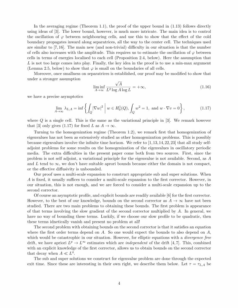
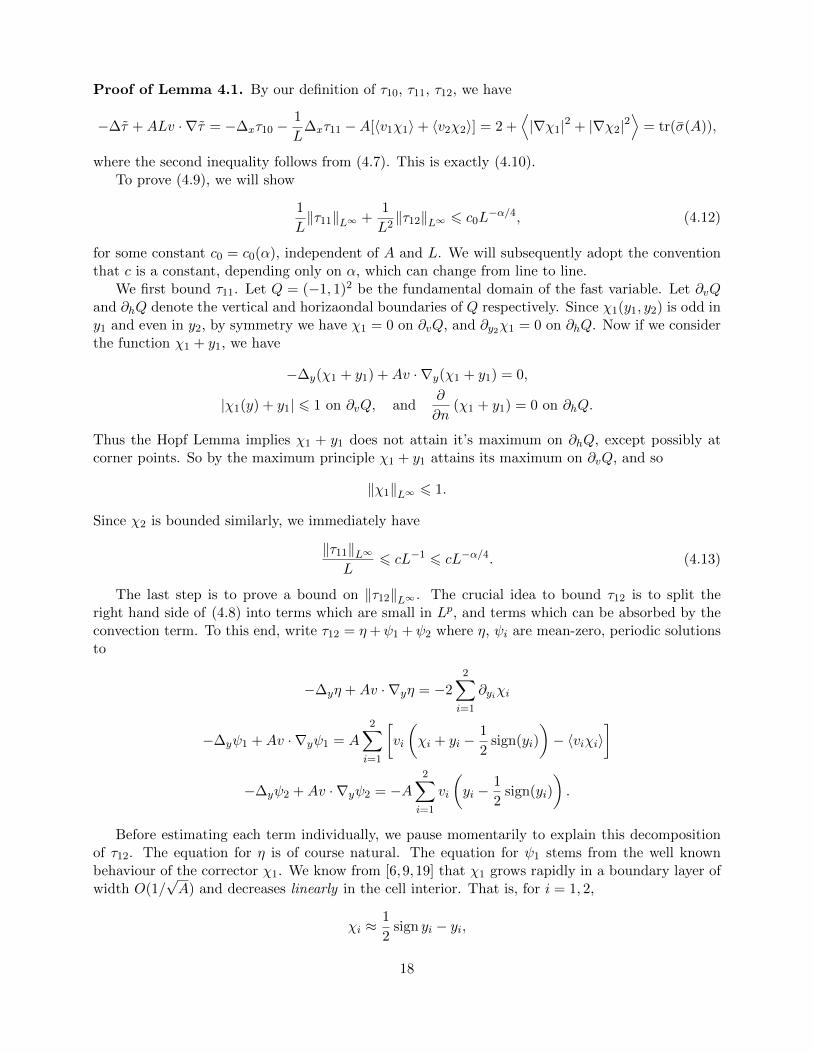
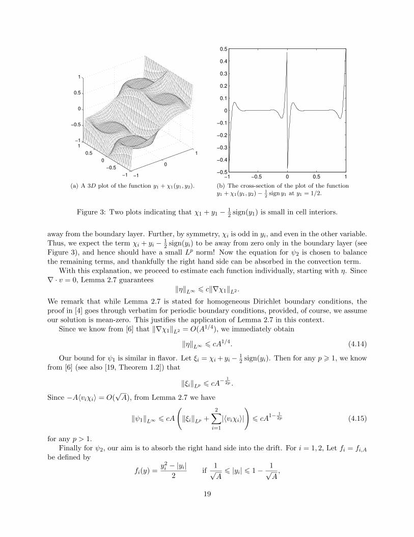
Before estimating each term individually, we pause momentarily to explain this decompositionof τ12. The equation for η is of course natural. The equation for ψ1 stems from the well knownbehaviour of the corrector χ1. We know from [6,9,19] that χ1 grows rapidly in a boundary layer ofwidth O(1/
√A) and decreases linearly in the cell interior. That is, for i = 1, 2,
χi ≈1
2sign yi − yi,
18
−1
0
1
−1
−0.5
0
0.5
1
−1
−0.5
0
0.5
1
(a) A 3D plot of the function y1 + χ1(y1, y2).
−1 −0.5 0 0.5 1−0.5
−0.4
−0.3
−0.2
−0.1
0
0.1
0.2
0.3
0.4
0.5
(b) The cross-section of the plot of the functiony1 + χ1(y1, y2) − 1
2sign y1 at y1 = 1/2.
Figure 3: Two plots indicating that χ1 + y1 − 12 sign(y1) is small in cell interiors.
away from the boundary layer. Further, by symmetry, χi is odd in yi, and even in the other variable.Thus, we expect the term χi + yi − 1
2 sign(yi) to be away from zero only in the boundary layer (seeFigure 3), and hence should have a small Lp norm! Now the equation for ψ2 is chosen to balancethe remaining terms, and thankfully the right hand side can be absorbed in the convection term.
With this explanation, we proceed to estimate each function individually, starting with η. Since∇ · v = 0, Lemma 2.7 guarantees
‖η‖L∞ 6 c‖∇χ1‖L2 .
We remark that while Lemma 2.7 is stated for homogeneous Dirichlet boundary conditions, theproof in [4] goes through verbatim for periodic boundary conditions, provided, of course, we assumeour solution is mean-zero. This justifies the application of Lemma 2.7 in this context.
Since we know from [6] that ‖∇χ1‖L2 = O(A1/4), we immediately obtain
‖η‖L∞ 6 cA1/4. (4.14)
Our bound for ψ1 is similar in flavor. Let ξi = χi + yi− 12 sign(yi). Then for any p > 1, we know
from [6] (see also [19, Theorem 1.2]) that
‖ξi‖Lp 6 cA− 1
2p .
Since −A〈viχi〉 = O(√A), from Lemma 2.7 we have
‖ψ1‖L∞ 6 cA
(‖ξi‖Lp +
2∑i=1
|〈viχi〉|
)6 cA
1− 12p (4.15)
for any p > 1.Finally for ψ2, our aim is to absorb the right hand side into the drift. For i = 1, 2, Let fi = fi,A
be defined by
fi(y) =y2i − |yi|
2if
1√A
6 |yi| 6 1− 1√A,
19
and extended to be a C1, periodic function on R2 in the natural way. Set θ = ψ2 +∑2
i=1(fi− 〈fi〉),then θ is a periodic, mean-zero solution to
−∆yθ +Av · ∇yθ =2∑i=1
(Avigi −∆yfi) .
where
gi(y) = ∂yifi − yi +1
2sign(yi)
Since for any p > 1, we can explicitly compute
‖gi‖Lp 6 cA− 1
2p and ‖∆yfi‖Lp 6 cA12− 1
2p ,
by Lemma 2.7 we obtain
‖ψ2‖L∞ 6 1 + ‖θ‖L∞ 6 cA1− 1
2p (4.16)
for any p > 1.Thus combining (4.14), (4.15) and (4.16), we see ‖τ12‖L∞ 6 cA1−1/(2p). Thus using (1.14) and
choosing p = 8−2α8−3α when 0 < α < 8/3, and p =∞ for α > 8/3, we see
‖τ12‖L∞L2
6 cL−α4
proving (4.12). This completes the proof.
Exit time from a square.
Theorem 1.4 follows immediately from Proposition 1.4.
Proof of Theorem 1.4. The proof of Theorem 1.4 is now trivial. We simply inscribe a disk D =|x| 6 L/2 into the square D = [−L/2, L/2]2, and circumscribe a bigger disk D = |x| 6 L/
√2
around D. The corresponding exit times satisfy the inequality
τ(x) 6 τ(x) 6 τ(x), for all x ∈ D.
Using the bounds obtained from Proposition 1.5 applied to D and D, the inequality (1.20) follows.
5 The eigenvalue in the homogenization regime
5.1 The lower bound
The lower bound for the eigenvalue stated in Theorem 1.2 follows, quickly from the upper boundon the expected exit time.
Proof of the lower bound in Theorem 1.2. We claim that in general, we have the principaleigenvalue and expected exit time satisfy
λ >1
‖τ‖L∞. (5.1)
20
To see this, pick any ε > 0, and suppose for contradiction that λ < 1/‖τ + ε‖L∞ . Then,
−∆(τ + ε) +Av · ∇(τ + ε) = 1 >1
‖τ + ε‖L∞(τ + ε) .
Also
−∆ϕ+Av · ∇ϕ = λϕ 61
‖τ + ε‖L∞ϕ.
Rescaling ϕ if necessary to ensure ‖ϕ‖L∞ 6 ε, we see have ϕ 6 τ + ε in D. Thus Perron’s methodimplies the existence of a function φ such that
−∆φ+Av · ∇φ =1
‖τ + ε‖L∞φ in D,
φ = 0 on ∂D,
ϕ 6 φ 6 τ in D
This immediately implies 1/‖τ + ε‖L∞ equals the principal eigenvalue λ, which contradicts ourassumption. Thus, for any ε > 0, we must have λ > 1/‖τ + ε‖L∞ . Sending ε→ 0, we obtain (5.1).Applying Theorem 1.4 concludes the proof.
5.2 The upper bound
In this section we prove the upper bound in Theorem 1.2. We will do this by using a multi-scaleexpansion of a sub-solution. As we have seen in the preceding sections, our multi-scale expansionsare all forced to use a quadratic ‘slow’ profile, in order to avoid extra terms in the expansion. Thismakes the construction of the sub-solution slightly more difficult. As customary with homogenizationproblems, we rescale the problem so that the cell size goes to 0, and the domain is fixed.
Lemma 5.1. Let h > 0, and ψ be the solution of−∆ψ +ALv(Lx) · ∇ψ = χB1−h in B1
ψ = 0 on ∂B1,(5.2)
where Br = |x| 6 r, and χS is the characteristic function of the set S. Assume that A and L varysuch that (1.14) holds. Then there exists h > 0, and c = c(h) > 0 such that
ψ(x) >c√A
for all x ∈ B1−h. (5.3)
provided A and L are sufficiently large.
Lemma 5.1 immediately implies the desired upper bound. We present this argument belowbefore delving into the technicalities of Lemma 5.1.
Proof of the upper bound in Theorem 1.2. Let ϕ1, µ1 be the principal eigenfunction and theprincipal eigenvalue respectively for the rescaled problem
−∆ϕ1 +ALv(Lx) · ∇ϕ1 = µ1ϕ1 in B1
ϕ1 = 0 on ∂B1,
ϕ1 > 0 in B1.
(5.4)
21
Assume, for contradiction, µ1 >√Ac , where c is the constant in Lemma 5.1, then
−∆ϕ1 +ALv(Lx) · ∇ϕ1 = µ1ϕ1 >
√A
cϕ1.
Also, if ψ is the function from Lemma 5.1, then by the maximum principle, ψ > 0 in B1−h. Hence,
−∆ψ +ALv(Lx) · ∇ψ = χB1−h 6
√A
cψ.
By the Hopf lemma, we know ∂ϕ1
∂n < 0 on ∂B1, and so ϕ1 can be rescaled to ensure ϕ1 > ψ. Perron’smethod now implies that there exists a function φ that satisfies
−∆φ+ALv(Lx) · ∇φ =
√A
cφ in B1
φ = 0 on ∂B1,
φ > 0 in B1,
(5.5)
and, in addition, ψ(x) 6 φ(x) 6 ϕ1(x). Therefore, µ1 =√A/c is the principal eigenvalue, which
contradicts our assumption µ1 >√A/c. Hence µ1 6
√A/c.
Now rescaling back so the cell size is 1, let λ′ and φ′ be the principal eigenvalue and principaleigenfunction respectively of the problem (1.11) on the ball of radius L/2. Since λ′ = 4µ1/L
2, wehave λ′ 6 4
√A/(cL2). Finally, let D be the square with side length L, and λ, ϕ are the principal
eigenvalue and eigenfunction respectively of the problem (1.11) on D. Then, since BL/2 ⊂ D, theprincipal eigenvalues must satisfy λ 6 λ′, from which the theorem follows.
It remains to prove Lemma 5.1.
Proof of Lemma 5.1. Let θ = τ1 − ψ, where τ1 is the solution of (4.1), the expected exit timeproblem from the unit disk. Now rescaling (1.21) to the ball of radius 1, (or directly using (4.11),which was what lead to (1.21)), we obtain∣∣∣∣τ1(x)− 1
2 tr(σ(A))
(1− |x|2
)∣∣∣∣ 6 c3L−α/4√A
(5.6)
provided A and L are large enough and satisfy (1.14). Here c3 > 0 is a fixed constant independentof A and L. Thus, (5.3) will follow if we show that
‖θ‖L∞(B1−h) 6 (1− ε′) infx∈B1−h
τ1(x) (5.7)
for some small ε′ > 0. Observe that (5.6) implies that the right hand side of (5.7) is O(h/√A).
Therefore, to establish (5.7), it suffices to show that there exists constants h0 > 0 and c > 0 suchthat for all h 6 h0, there exists A0 = A0(h) and L0 = L0(h) such that
‖θ‖L∞(B1−h) 6c√Ah3/2, (5.8)
provided A > A0, L > L0 and (1.14) holds. Above any power of h strictly larger than 1 will do; ourconstruction below obtains h3/2, however, in reality one would expect the power to be h2.
We will obtain (5.8) by considering a Poisson problem on the annulus
A1−2h,1 = 1− 2h 6 |x| 6 1.
22
If we impose a large enough constant boundary condition on the inner boundary, the (inward) normalderivative will be negative on ∂B1−2h. Now, if we extend this function inward by a constant, wewill have a super-solution giving the desired estimate for θ(x). We first state a lemma guaranteeingthe sign of the normal derivative of an appropriate Poisson problem.
Lemma 5.2. There exists h0 and c2 > 0, such that for all h < h0, there exists A0, L0 > 0 suchthat the solution θ1 of the PDE
−∆θ1 +ALv(Lx) · ∇θ1 = χA1,1−h in A1−2h,1
θ1 = 0 on ∂B1,
θ1 =c2√Ah3/2 on ∂B1−2h,
(5.9)
satisfies∂θ1
∂r6 0 on ∂B1−2h,
provided L > L0, A > A0 and (1.14) holds. Here ∂∂r denotes the derivative with respect to the radial
direction. Moreover, the function θ1 attains its maximum on |x| = 1− 2h, and θ1(x) 6 c2h3/2/√A
for all x ∈ A1−2h,1.
Now, postponing the proof of Lemma 5.2, we prove (5.8). Choose h small, and A,L large, asguaranteed by Lemma 5.2, and define θ by
θ(x) =
θ1(x) when |x| > 1− 2hc2√Ah3/2 when |x| < 1− 2h.
where θ1 and c2 are as in Lemma 5.2. Then θ ∈ C(B1) ∩ C2(B1−2h ∪ A1−2h,1), and
(−∆ +ALv(Lx) · ∇) θ(x) =
1 when |x| > 1− h0 when |x| < 1− h & |x| 6= 1− 2h
Further, when |x| = 1− 2h,∂θ
∂r−= 0 and
∂θ
∂r+6 0
where the second inequality follows from Lemma 5.2. Thus θ is a viscosity super solution to thePDE
−∆θ +ALv(Lx) · ∇θ = χA1,1−h in B1
θ = 0 on ∂B1.
By the comparison principle, we must have θ > θ, which immediately proves (5.8). From this (5.7)follows, and using (5.6) we obtain (5.2), concluding the proof.
It remains to prove Lemma 5.2. Roughly speaking, if we choose the constant c2 sufficientlylarge, the function θ1 is nearly harmonic. The inhomogeneity of the boundary conditions dominatesthe right side of the equation. A “nearly harmonic” function should attain its maximum on theboundary, implying the conclusion of Lemma 5.2.
The reason we believe the constant c2h3/2/√A is large enough, is because the homogenized exit
time from the annulus is quadratic in the width of the annulus. Unfortunately, the slow profile
23
is not quadratic in Cartesian coordinates, and so the best we can do is obtain upper and lowerbounds, which need not be sharp. We begin by showing that the expected exit time from anannulus of width h grows like h3/2. While we certainly don’t expect the exponent 3/2 to be sharp,any exponent strictly larger than 1 will suffice for our needs.
Lemma 5.3. Let A1−h,1 be the annulus A1−h,1def= B1\B1−h, and τann be the solution of the Poisson
problem −∆τann +ALv(Lx) · ∇τann = 1 in A1−h,1
τann = 0 on ∂A1−h,1(5.10)
Suppose L and A vary so that (1.14) holds. Then there exists constants h0 > 0 and c > 0 such thatfor all h < h0, there exists A0 = A0(h) and L0 = L0(h) such that
‖τann‖L∞(A1−h,1) 6c1√Ah3/2
provided L > L0, A > A0 and (1.14) holds.
Proof. The main idea behind the proof is that as A,L→∞, we know that τ1 tends to an explicit(homogenized) parabolic profile and is constant on ∂B1−h. Now if we subtract off a harmonicfunction with these boundary values, then we should get a super solution for τann. Finally, we willshow that a harmonic function with constant boundary values grows linearly near ∂B1, at the samerate as τ1. Thus the above super solution will give an upper bound for τann which is super-linear inthe annulus width.
We proceed to carry out the details. Let η′ be the solution of−∆η′ +ALv(Lx) · ∇η′ = 0 in A1−h,1
η′ = 0 on ∂B1
η′ =2h− h2
2 tr(σ(A))on ∂B1−h,
(5.11)
and define
τann = τ1 − η′ +c3L−α/4√A
,
where c3 is as in (5.6). Then τann satisfies−∆τann +ALv(Lx) · ∇τann = 1 in A1−h,1
τann > 0 on ∂B1
τann > 0 on ∂B1−h.
The first boundary condition follows because both η′ and τ1 are 0 on ∂B1. The second followsfrom (5.6) and the boundary condition for η′. Thus, the maximum principle immediately impliesthat τann > τann.
Since (5.6) gives the asymptotics for τ1, to conclude the proof we need a lower bound on η′ thatis ‘linear’ in the radial direction near ∂B1. We separate this estimate as a lemma.
Lemma 5.4. Let η be the solution of−∆η +ALv(Lx) · ∇η = 0 in A1−h,1
η = 0 on ∂B1
η = h on ∂B1−h,
(5.12)
24
Then there exists a constant c, independent of h, A and L, such that
η(x) > 1− |x| − c
(h3/2 +
L−α/4√h
)(5.13)
when L and A are sufficiently large.
Returning to the proof of Lemma 5.3, we see that Lemma 5.4 gives
η′(x) >2− h
2 tr(σ(A))
[1− |x| − c
(h3/2 +
L−α/4√h
)].
Now using the above and (1.8), it follows that
τann(x) 6 τann(x) = τ1(x)− η′(x) +cL−α/4√
A
61
2 tr(σ(A))
(1− |x|2 − (2− h)(1− |x|) + ch3/2
)+
1√A
(cL−α/4 +
cL−α/4√h
)
=1
2 tr(σ(A))
((1− |x|) (h− (1− |x|)) + ch3/2
)+
1√A
(cL−α/4√
h
)
61
2 tr(σ(A))
(h2 + ch3/2
)+
1√A
(cL−α/4√
h
)obtaining Lemma 5.3 as desired.
To complete the proof of Lemma 5.3, we need to prove Lemma 5.4. We do this next.
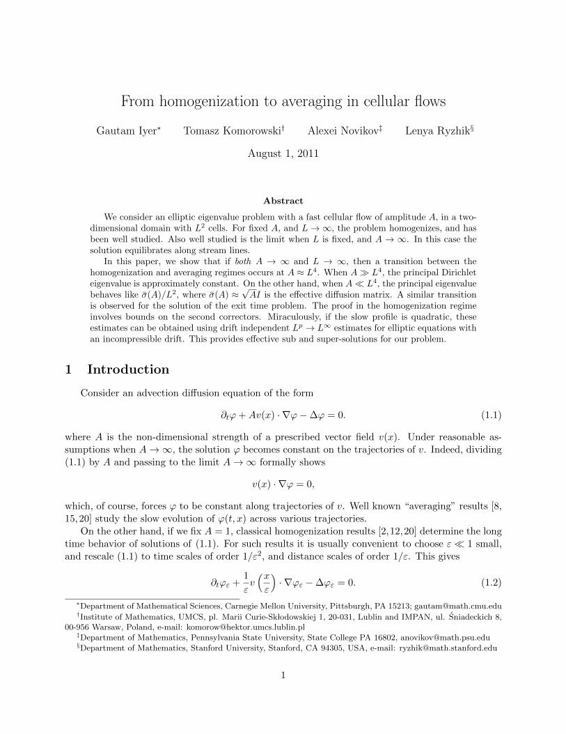
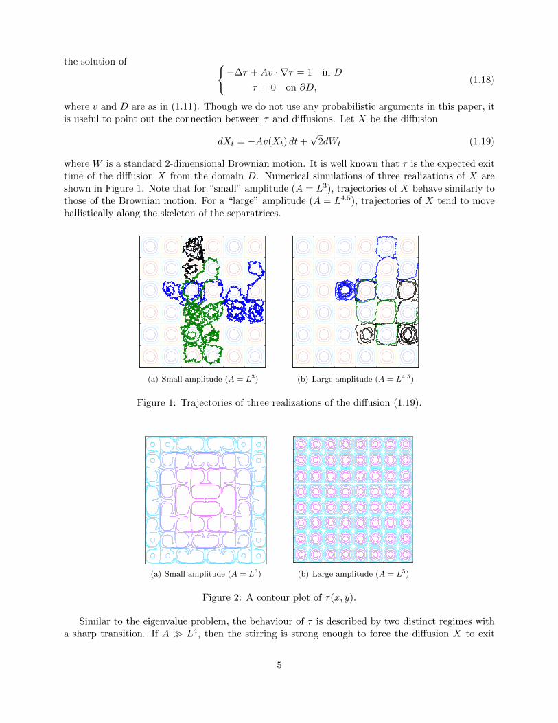
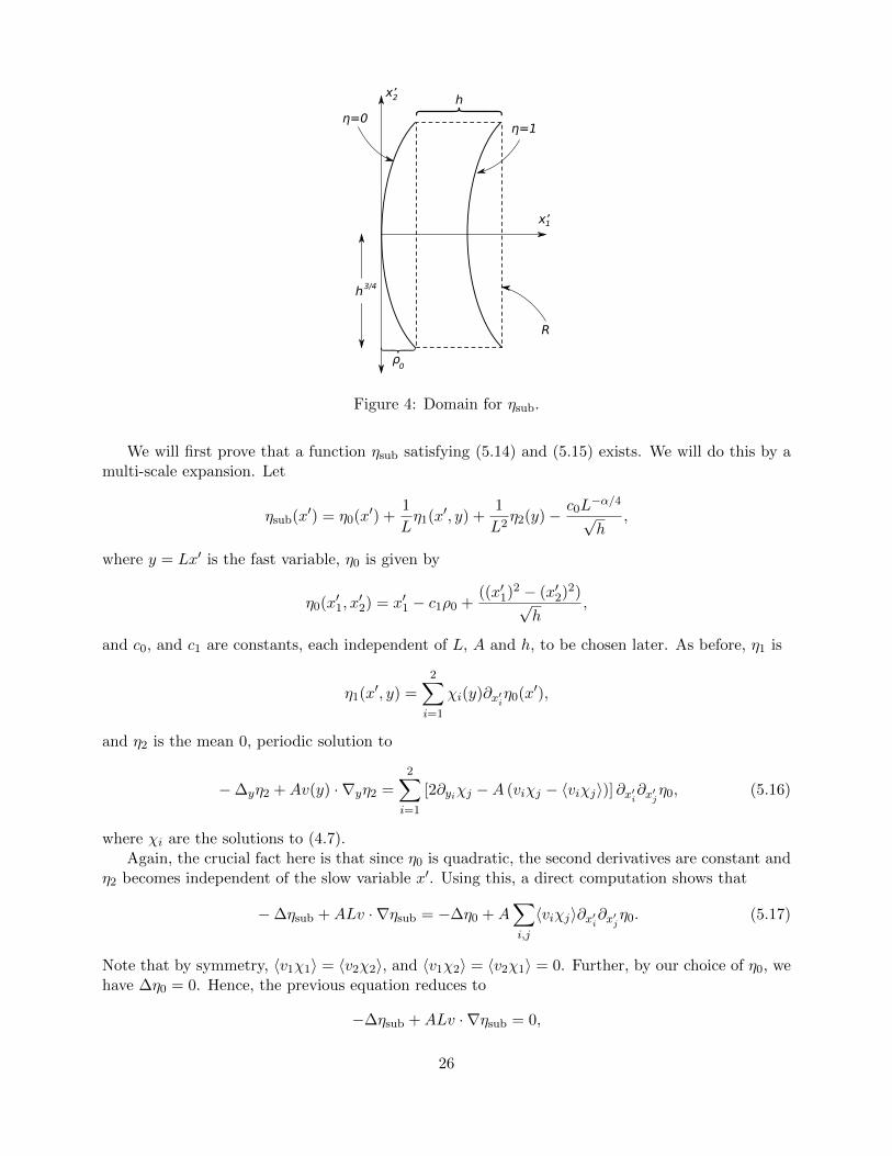
Proof of Lemma 5.4. We will construct a sub-solution of equation (5.12) in small rectangles over-lapping A1−h,1. For convenience, we now shift the origin to (−1, 0), and consider new coordinates
(x′1, x′2)
def= (x1 + 1, x2). In these coordinates, let R be the rectangle of height 2h3/4, width h and
top left corner (ρ0, h3/4), where ρ0 = 1− (1− h3/2)1/2 (see Figure 4).
We will construct a function ηsub such that−∆ηsub +ALv(Lx) · ∇ηsub = 0 in A1−h,1,
ηsub 6 h on the right boundary of R,
ηsub 6 0 on the other three boundaries of R,
(5.14)
and ηsub satisfies the linear growth condition
ηsub(x′1, 0) > x′1 − c
(h3/2 +
L−α/4√h
)when x′1 ∈ [ρ0, ρ0 + h], (5.15)
for some constant c independent of L, A and h.Before proving that the function ηsub exists, we remark that by the maximum principle, we
ηsub 6 η on R ∩ A1−h,h. Moreover, as ρ0 = O(h3/2), the estimate (5.13) can be extended tox′1 ∈ [0, ρ0] as well, possibly by increasing the constant c. This proves Lemma 5.4 when x is onthe negative x1-axis. Now, if (5.15) is still valid when the coordinate frame is rotated, our proof ofLemma 5.4 will be complete!
25
η=0η=1
R
h3/4
x’1
x’2
ρ0
⎧ ⎨ ⎩
h ⎧⎪⎨⎪⎩
Figure 4: Domain for ηsub.
We will first prove that a function ηsub satisfying (5.14) and (5.15) exists. We will do this by amulti-scale expansion. Let
ηsub(x′) = η0(x′) +1
Lη1(x′, y) +
1
L2η2(y)− c0L
−α/4√h
,
where y = Lx′ is the fast variable, η0 is given by
η0(x′1, x′2) = x′1 − c1ρ0 +
((x′1)2 − (x′2)2)√h
,
and c0, and c1 are constants, each independent of L, A and h, to be chosen later. As before, η1 is
η1(x′, y) =2∑i=1
χi(y)∂x′iη0(x′),
and η2 is the mean 0, periodic solution to
−∆yη2 +Av(y) · ∇yη2 =2∑i=1
[2∂yiχj −A (viχj − 〈viχj〉)] ∂x′i∂x′jη0, (5.16)
where χi are the solutions to (4.7).Again, the crucial fact here is that since η0 is quadratic, the second derivatives are constant and
η2 becomes independent of the slow variable x′. Using this, a direct computation shows that
−∆ηsub +ALv · ∇ηsub = −∆η0 +A∑i,j
〈viχj〉∂x′i∂x′jη0. (5.17)
Note that by symmetry, 〈v1χ1〉 = 〈v2χ2〉, and 〈v1χ2〉 = 〈v2χ1〉 = 0. Further, by our choice of η0, wehave ∆η0 = 0. Hence, the previous equation reduces to
−∆ηsub +ALv · ∇ηsub = 0,
26
as required by the first equation in (5.14).Next, we show that if c1 is appropriately chosen, we can arrange the boundary conditions claimed
in (5.14) for η0. Notice that ρ0 = O(h3/2), and on the top and bottom boundary we have x′2 = ±h3/4
and x′1 ∈ (ρ0, ρ0 + h). Thus
x′1 −(x′2)2
√h
6 ρ0 and(x′1)2
√h
6 O(h3/2).
So choosing c1 large enough, we can ensure η0 6 0 on the top and bottom of R.On the left of R, we have x′1 = ρ0 and |x2| 6 h3/4. So (x′1)2/
√h 6 O(h5/2) = o(ρ0), and choosing
c1 large we can again ensure η0 6 0 on the left of R. Finally, on the right of R, we have x′1 = ρ0 +hand |x′2| 6 h3/4, and we immediately see that for c1 large enough, we have η0 6 h on the right of R.Thus η0 satisfies the boundary conditions in (5.14).
To see that ηsub also satisfies the boundary conditions in (5.14), we need to bound the correctorsappropriately. Exactly as in the proof of Lemma 4.1, we obtain∥∥∥∥ 1
Lη1 +
1
L2η2
∥∥∥∥L∞
6cL−α/4√
h, (5.18)
where c > 0 is independent of L, A and h. We remark that the extra 1/√h factor arises because
derivatives of η0 are of the order 1/√h and they appear as multiplicative factors in the expressions
for η1 and η2.Consequently, if c0 is chosen to be larger than c, we have
1
Lη1 +
1
L2η2 −
c0L−α/4√h
6 0. (5.19)
Since η0 already satisfies the boundary conditions in (5.14), this immediately implies that ηsub
must also satisfy these boundary conditions. Finally, since η0 certainly satisfies (5.15), it followsfrom (5.19) that ηsub also satisfies (5.15). This proves the existence of ηsub.
Now, as remarked earlier, the only thing remaining to complete the proof of the Lemma is toverify that if the rectangle R, and the coordinate frame are both rotated arbitrarily about the centerof the annulus, then there still exists a function ηsub satisfying (5.14) and (5.15) in new coordinates.This, however, is immediate. The new coordinates can be expressed in terms of the old coordinatesas a linear function. Consequently, our initial profile for η0 will still be a quadratic function of thenew coordinates. Of course, by the rotational invariance of the Laplacian, it will also be harmonic,and the remainder of the proof goes through nearly verbatim. The only modification is that afterthe rotation the mixed derivative ∂x′1∂x′2η0 no longer vanishes, and the terms involving v1χ2 andv2χ1 do appear in (5.16) and (5.17). However, they can be treated in an identical fashion, as inthe proof of Lemma 4.1 using the precise asymptotics for χ1 and χ2 from [19]. This concludes theproof.
Finally, we are ready for the proof of Lemma 5.2.
Proof of Lemma 5.2. For a given c2, let η′ be the solution of−∆η′ +ALv(Lx) · ∇η′ = 0 in A1−2h,1
η′ = 0 on ∂B1
η′ =c2√Ah3/2 on ∂B1−2h,
27
Then, we haveθ1 − η′ = 0 on ∂A1−2h,1,
and−∆θ1 +ALv(Lx) · ∇θ1 6 1 in A1−2h,1.
Consequently θ1 − η′ 6 τann, where τann is the solution of (5.10) on the annulus A1−2h,1. Thusapplying Lemma 5.3, we see
θ1(x) 6c1√A
(2h)3/2 + η′(x) (5.20)
The function η′ decreases at most linearly with |x|. This can be seen immediately from anasymptotic expansion for a super solution. Indeed, starting with
η0(x) =c2
√h
2√A
(1− x1)
and choosing η1 and η2 as in the proof of Lemma 5.4, we immediately see that
η′(x1, 0) 6c2
√h
2√A
(1− x1) + c√hA−1/2L−α/4.
We remark again that the extra√hA−1/2 factor arises from the gradient of η0. Now by rotating the
initial profile η0 appropriately, we obtain the linear decrease
η′(x) 6c2
√h
2√A
(1− |x|) + c√hA−1/2L−α/4. (5.21)
as claimed.We claim that (5.20) and (5.21) quickly conclude the proof. To see this, note first that equa-
tion (5.20) and (5.21) immediately give
θ1(x) 6c1√A
(2h)3/2 +c2
2√Ah3/2 + c
√hA−1/2L−α/4 whenever x ∈ A1−h,1. (5.22)
However, since−∆θ1 +ALv(Lx) · ∇θ1 = 0
on A1−2h,1−h, the maximum principle implies that θ1 can not attain it’s maximum in the interior ofthe annulus A1−2h,1−h. Consequently (5.22) must hold on the interior of the entire annulus A1−2h,1.
Now if we choose c2 large enough so that 23/2c1 <c24 , and then choose L,A large enough so that
cA−1/2L−α/4 < c24 , we see that θ1 is forced to attain it’s maximum on the inner boundary ∂B1−2h,
and the Lemma follows immediately.
References
[1] G. Allaire and Y. Capdeboscq, Homogenization of a spectral problem in neutronic multigroup diffusion, Comput.Methods Appl. Mech. Engrg. 187 2000, no. 1-2, 91–117.
[2] A. Bensoussan, J.-L. Lions, and G. Papanicolaou, Asymptotic analysis for periodic structures, Studies in Mathe-matics and its Applications, vol. 5, North-Holland Publishing Co., Amsterdam, 1978.
[3] H. Berestycki, F. Hamel, and N. Nadirashvili, Elliptic eigenvalue problems with large drift and applications tononlinear propagation phenomena, Comm. Math. Phys. 253 2005, no. 2, 451–480.
[4] H. Berestycki, A. Kiselev, A. Novikov, and L. Ryzhik, Explosion problem in a flow, to appear.
28
[5] S. Childress, Alpha-effect in flux ropes and sheets, Phys. Earth Planet Inter. 20 1979, 172–180.
[6] A. Fannjiang and G. Papanicolaou, Convection enhanced diffusion for periodic flows, SIAM J. Appl. Math. 541994, no. 2, 333–408.
[7] A. Fannjiang, A. Kiselev, and L. Ryzhik, Quenching of reaction by cellular flows, Geom. Funct. Anal. 16 2006,no. 1, 40–69.
[8] M. I. Freidlin and A. D. Wentzell, Random perturbations of dynamical systems, 2nd ed., Grundlehren der Math-ematischen Wissenschaften [Fundamental Principles of Mathematical Sciences], vol. 260, Springer-Verlag, NewYork, 1998. Translated from the 1979 Russian original by Joseph Szucs.
[9] Y. Gorb, D. Nam, and A. Novikov, Numerical simulations of diffusion in cellular flows at high Peclet numbers,Discrete Contin. Dyn. Syst. Ser. B 15 2011, no. 1, 75–92.
[10] S. Heinze, Diffusion-advection in cellular flows with large Peclet numbers, Arch. Ration. Mech. Anal. 168 2003,no. 4, 329–342.
[11] G. Iyer, A. Novikov, L. Ryzhik, and A. Zlatos, Exit times for diffusions with incompressible drift, SIAM J. Math.Anal. 2010, to appear, available at arXiv:0911.2294.
[12] V. V. Jikov, S. M. Kozlov, and O. A. Oleınik, Homogenization of differential operators and integral functionals,Springer-Verlag, Berlin, 1994. Translated from the Russian by G. A. Yosifian [G. A. Iosif′yan].
[13] S. Kesavan, Homogenization of elliptic eigenvalue problems. I, Appl. Math. Optim. 5 1979, no. 2, 153–167 (English,with French summary).
[14] S. Kesavan, Homogenization of elliptic eigenvalue problems. II, Appl. Math. Optim. 5 1979, no. 3, 197–216(English, with French summary).
[15] Y. Kifer, Random perturbations of dynamical systems, Progress in Probability and Statistics, vol. 16, BirkhauserBoston Inc., Boston, MA, 1988.
[16] A. Kiselev and L. Ryzhik, Enhancement of the traveling front speeds in reaction-diffusion equations with advection,Ann. Inst. H. Poincare Anal. Non Lineaire 18 2001, no. 3, 309–358 (English, with English and French summaries).
[17] L. Koralov, Random perturbations of 2-dimensional Hamiltonian flows, Probab. Theory Related Fields 129 2004,no. 1, 37–62.
[18] A. J. Majda and P. R. Kramer, Simplified models for turbulent diffusion: theory, numerical modelling, and physicalphenomena, Phys. Rep. 314 1999, no. 4-5, 237–574.
[19] A. Novikov, G. Papanicolaou, and L. Ryzhik, Boundary layers for cellular flows at high Peclet numbers, Comm.Pure Appl. Math. 58 2005, no. 7, 867–922.
[20] G. A. Pavliotis and A. M. Stuart, Multiscale methods, Texts in Applied Mathematics, vol. 53, Springer, New York,2008. Averaging and homogenization.
[21] M. N. Rosenbluth, H. L. Berk, I. Doxas, and W. Horton, Effective diffusion in laminar convective flows, Phys.Fluids 30 1987, 2636–2647.
[22] F. Santosa and M. Vogelius, First-order corrections to the homogenized eigenvalues of a periodic composite medium,SIAM J. Appl. Math. 53 1993, no. 6, 1636–1668.
[23] F. Santosa and M. Vogelius, Erratum to the paper: “First-order corrections to the homogenized eigenvalues ofa periodic composite medium” [SIAM J. Appl. Math. 53 (1993), no. 6, 1636–1668; MR1247172 (94h:35188)],SIAM J. Appl. Math. 55 1995, no. 3, 864.
[24] B. Shraiman, Diffusive transport in a Raleigh-Bernard convection cell, Phys. Rev. A 36 1987, 261–267.
[25] P. B. Rhines and W. R. Young, How rapidly is passive scalar mixed within closed streamlines?, J. Fluid Mech.133 1983, 135–145.
29