CHAPTER 5: STATIONARY PERTURBATION THEORY

(From Cohen-Tannoudji, Chapter XI)

A. DESCRIPTION OF THE METHOD

Approximation methods to obtain analytical solution of eigenvalue problems.

1. Statement of the problem

We consider a time-independent perturbation

H = H0 + W (5.1)

of the time-independent Hamiltonian H0, whose eigenvalues and eigenvectors areknown and which captures the essential physics, by an additional term

W = λW (5.2)

λ � 1 (5.3)

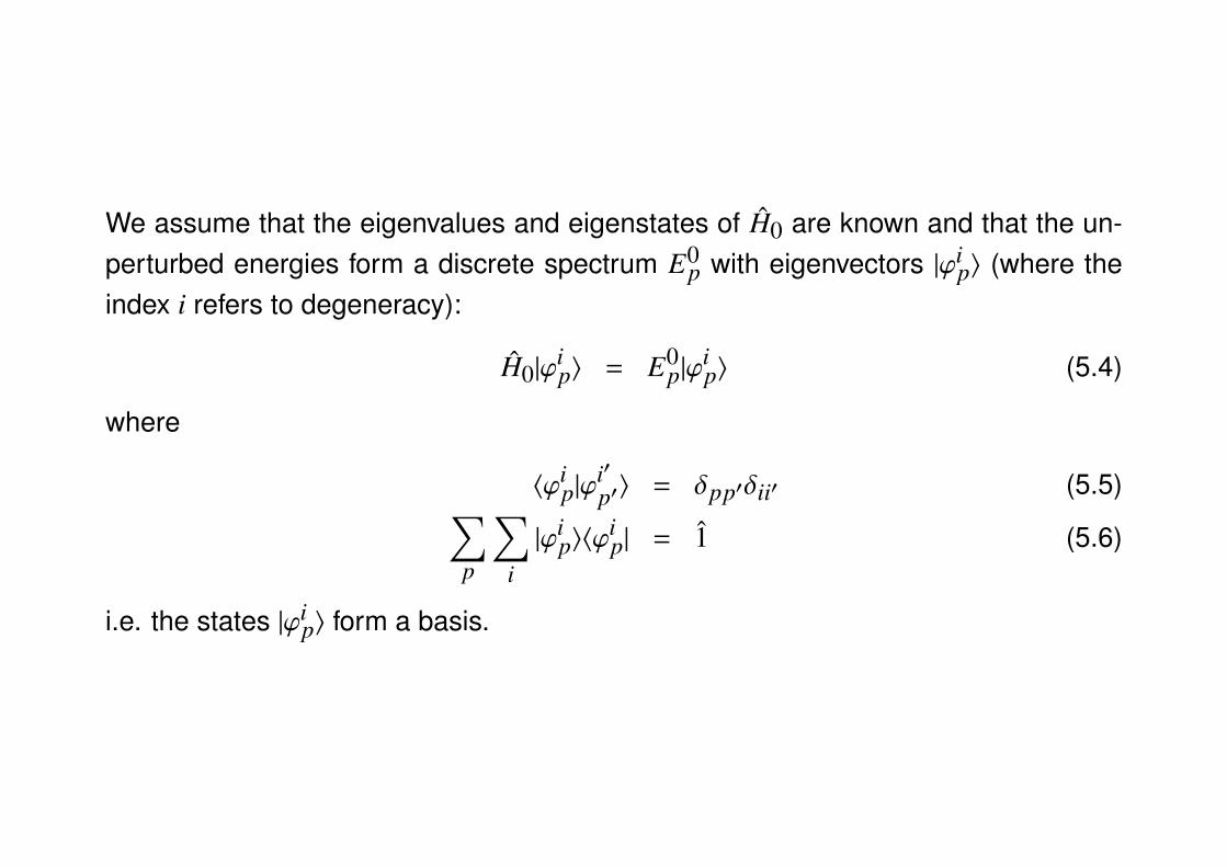
We assume that the eigenvalues and eigenstates of H0 are known and that the un-perturbed energies form a discrete spectrum E0

p with eigenvectors |ϕip〉 (where the

index i refers to degeneracy):

H0|ϕip〉 = E0

p|ϕip〉 (5.4)

where

〈ϕip|ϕ

i′p′〉 = δpp′δii′ (5.5)∑

p

∑i|ϕi

p〉〈ϕip| = 1 (5.6)

i.e. the states |ϕip〉 form a basis.

We seek an approximative solution of the full Hamiltonian H(λ) = H0 + λW

H(λ)|ψ(λ)〉 = E(λ)|ψ(λ)〉 (5.7)

where the eigenvalue and eigenvector can be expanded in terms of λ

E(λ) = ε0 + λε1 + . . . + λqεq + . . . (5.8)

|ψ(λ)〉 = |0〉 + λ|1〉 + . . . + λq|q〉 + . . . (5.9)

Inserting these into the eigenvalue equation yields

(H0 + λW

) ∞∑q=0

λq|q〉

=

∞∑q′=0

λq′εq′

∞∑q=0

λq|q〉

(5.10)

As this equation must hold for any (small) value of λ, it must hold for each power ofλ separately, giving the equations for various orders of the perturbation:0th-order: is just the eigenvalue equation of the unperturbed Hamiltonian, ε0 = E0

n

H0|0〉 = ε0|0〉 (5.11)

1st order: (H0 − ε0

)|1〉 +

(W − ε1

)|0〉 = 0 (5.12)

2nd order (H0 − ε0

)|2〉 +

(W − ε1

)|1〉 − ε2|0〉 = 0 (5.13)

q-th order (H0 − ε0

)|q〉 +

(W − ε1

)|q − 1〉 − ε2|q − 2〉 . . . − εq|0〉 = 0 (5.14)

We shall write |ψ(λ)〉 to be normalized and its phase will be chosen s.t. 〈0|ψ(λ)〉 ∈ R.For 0th order we have

〈0|0〉 = 1 (5.15)

and to the 1st order we get

〈ψ(λ)|ψ(λ)〉 = [〈0| + λ〈1|] [|0〉 + λ|1〉] + O(λ2

)(5.16)

= 〈0|0〉 + λ [〈1|0〉 + 〈0|1〉] + O(λ2

)(5.17)

Since both 〈0|0〉 = 1 and 〈ψ(λ)|ψ(λ)〉 = 1 we get to the 1st order

λ [〈1|0〉 + 〈0|1〉] = 0

⇒ 〈0|1〉 = 〈1|0〉 = 0 (5.18)

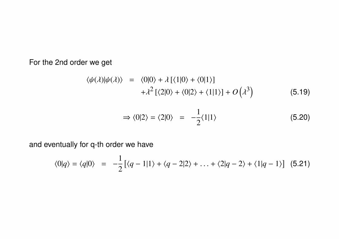
For the 2nd order we get

〈ψ(λ)|ψ(λ)〉 = 〈0|0〉 + λ [〈1|0〉 + 〈0|1〉]

+λ2 [〈2|0〉 + 〈0|2〉 + 〈1|1〉] + O(λ3

)(5.19)

⇒ 〈0|2〉 = 〈2|0〉 = −12〈1|1〉 (5.20)

and eventually for q-th order we have

〈0|q〉 = 〈q|0〉 = −12[〈q − 1|1〉 + 〈q − 2|2〉 + . . . + 〈2|q − 2〉 + 〈1|q − 1〉

](5.21)

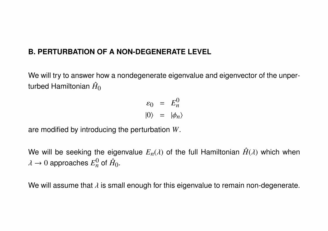
B. PERTURBATION OF A NON-DEGENERATE LEVEL

We will try to answer how a nondegenerate eigenvalue and eigenvector of the unper-turbed Hamiltonian H0

ε0 = E0n

|0〉 = |φn〉

are modified by introducing the perturbation W.

We will be seeking the eigenvalue En(λ) of the full Hamiltonian H(λ) which whenλ→ 0 approaches E0

n of H0.

We will assume that λ is small enough for this eigenvalue to remain non-degenerate.

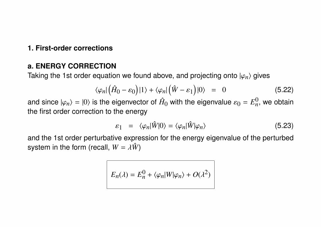
1. First-order corrections

a. ENERGY CORRECTIONTaking the 1st order equation we found above, and projecting onto |ϕn〉 gives

〈ϕn|(H0 − ε0

)|1〉 + 〈ϕn|

(W − ε1

)|0〉 = 0 (5.22)

and since |ϕn〉 = |0〉 is the eigenvector of H0 with the eigenvalue ε0 = E0n, we obtain

the first order correction to the energy

ε1 = 〈ϕn|W |0〉 = 〈ϕn|W |ϕn〉 (5.23)

and the 1st order perturbative expression for the energy eigenvalue of the perturbedsystem in the form (recall, W = λW)

En(λ) = E0n + 〈ϕn|W |ϕn〉 + O(λ2)

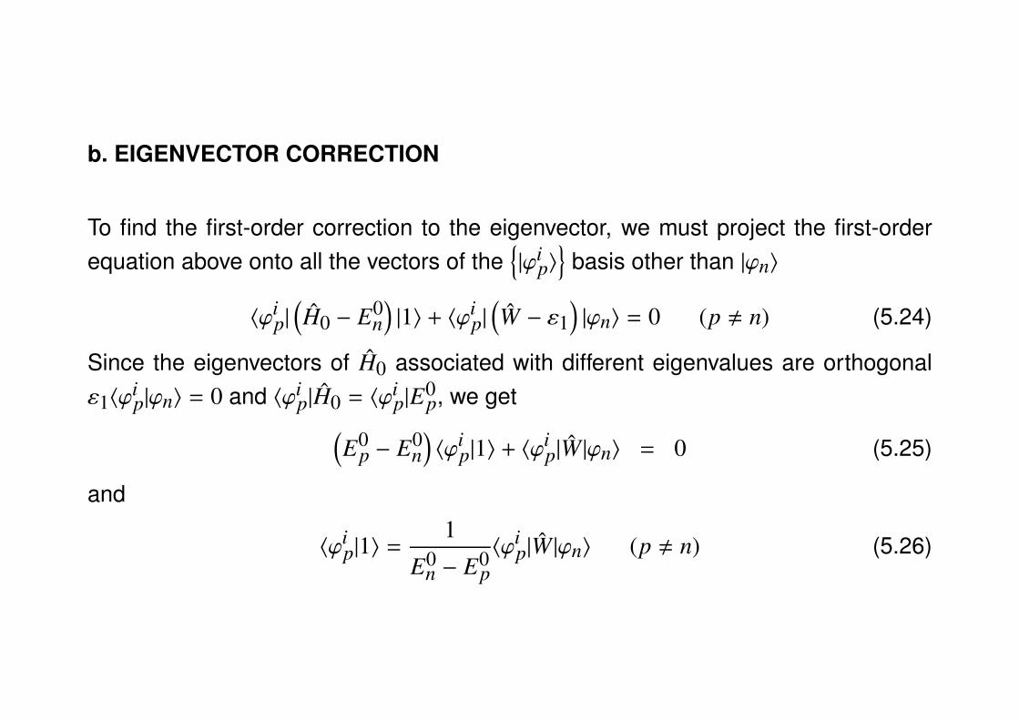
b. EIGENVECTOR CORRECTION

To find the first-order correction to the eigenvector, we must project the first-orderequation above onto all the vectors of the

{|ϕi

p〉}

basis other than |ϕn〉

〈ϕip|

(H0 − E0

n)|1〉 + 〈ϕi

p|(W − ε1

)|ϕn〉 = 0 (p , n) (5.24)

Since the eigenvectors of H0 associated with different eigenvalues are orthogonalε1〈ϕ

ip|ϕn〉 = 0 and 〈ϕi

p|H0 = 〈ϕip|E

0p, we get(

E0p − E0

n)〈ϕi

p|1〉 + 〈ϕip|W |ϕn〉 = 0 (5.25)

and

〈ϕip|1〉 =

1

E0n − E0

p〈ϕi

p|W |ϕn〉 (p , n) (5.26)

and, since 〈ϕn|1〉 = 〈0|1〉 = 0, the first order correction to the eigenvector can bewritten as

|1〉 =∑p,n

∑i

〈ϕip|W |ϕn〉

E0n − E0

p|ϕi

p〉 (5.27)

The expression for the eigenvector of the perturbed Hamiltonian to the first-order isthus

|ψn(λ)〉 = |ϕn〉 +∑p,n

∑i

〈ϕip|W |ϕn〉

E0n − E0

p|ϕi

p〉 + O(λ2

)(5.28)

The perturbation W mixes the state |φn〉 with the other eigenstates of H0.

2. Second-order corrections

a. ENERGY CORRECTION

We proceed in a way similar to the previous case. We project the 2nd order equationobtained above onto |ϕn〉

〈ϕn|(H0 − E0

n)|2〉 + 〈ϕn|

(W − ε1

)|1〉 − ε2〈ϕn|ϕn〉 = 0 (5.29)

Since |ϕn〉 = |0〉 is the eigenvector of H0 with the eigenvalue ε0 = E0n, the first term is

zero and the second order correction becomes

ε2 = 〈ϕn|W |1〉 (5.30)

With the expression for |1〉 obtained above we can write the second order correctionto the energy eigenvalue as

ε2 =∑p,n

∑i

∣∣∣〈ϕip|W |ϕn〉

∣∣∣2E0

n − E0p

(5.31)

The 2nd order expression for the energy eigenvalue of the perturbed system be-comes

En(λ) = E0n + 〈ϕn|W |ϕn〉 +

∑p,n

∑i

∣∣∣〈ϕip|W |ϕn〉

∣∣∣2E0

n − E0p

+ O(λ3) (5.32)

b. EIGENVECTOR CORRECTION

The eigenvector corrections |2〉 can be obtained by projecting the equation(H0 − ε0

)|2〉 +

(W − ε1

)|1〉 − ε2|0〉 = 0 (5.33)

onto the set of basis vectors |φip〉 different from |φn〉 and by using the condition

〈0|2〉 = 〈2|0〉 = −12〈1|1〉 (5.34)

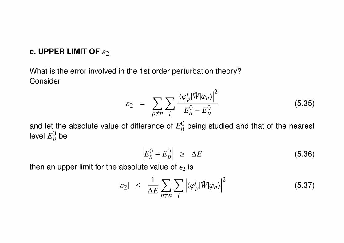
c. UPPER LIMIT OF ε2

What is the error involved in the 1st order perturbation theory?Consider

ε2 =∑p,n

∑i

∣∣∣〈ϕip|W |ϕn〉

∣∣∣2E0

n − E0p

(5.35)

and let the absolute value of difference of E0n being studied and that of the nearest

level E0p be ∣∣∣∣E0

n − E0p

∣∣∣∣ ≥ ∆E (5.36)

then an upper limit for the absolute value of ε2 is

|ε2| ≤1

∆E

∑p,n

∑i

∣∣∣∣〈ϕip|W |ϕn〉

∣∣∣∣2 (5.37)

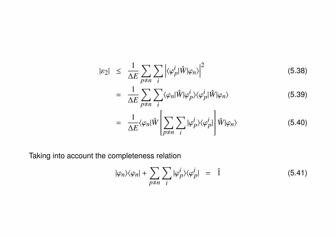
|ε2| ≤1

∆E

∑p,n

∑i

∣∣∣∣〈ϕip|W |ϕn〉

∣∣∣∣2 (5.38)

=1

∆E

∑p,n

∑i〈ϕn|W |ϕi

p〉〈ϕip|W |ϕn〉 (5.39)

=1

∆E〈ϕn|W

∑p,n

∑i|ϕi

p〉〈ϕip|

W |ϕn〉 (5.40)

Taking into account the completeness relation

|ϕn〉〈ϕn| +∑p,n

∑i|ϕi

p〉〈ϕip| = 1 (5.41)

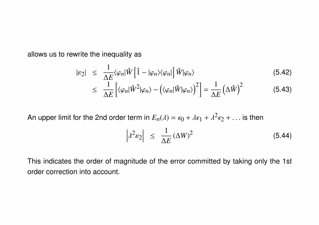
allows us to rewrite the inequality as

|ε2| ≤1

∆E〈ϕn|W

[1 − |ϕn〉〈ϕn|

]W |ϕn〉 (5.42)

≤1

∆E

[〈ϕn|W2|ϕn〉 −

(〈ϕn|W |ϕn〉

)2]

=1

∆E

(∆W

)2(5.43)

An upper limit for the 2nd order term in En(λ) = ε0 + λε1 + λ2ε2 + . . . is then∣∣∣∣λ2ε2

∣∣∣∣ ≤ 1∆E

(∆W)2 (5.44)

This indicates the order of magnitude of the error committed by taking only the 1storder correction into account.

C. PERTURBATION OF A DEGENERATE STATE

Assume that the level E0n to be gn-fold degenerate, and E0

n be the correspondinggn-fold dimensional eigenspace of H0.

Now the choice

ε0 = E0n (5.45)

is not sufficient to determine |0〉 since the equation H0|0〉 = ε0|0〉can be satisfied byany linear combination of vectors in E0

n.

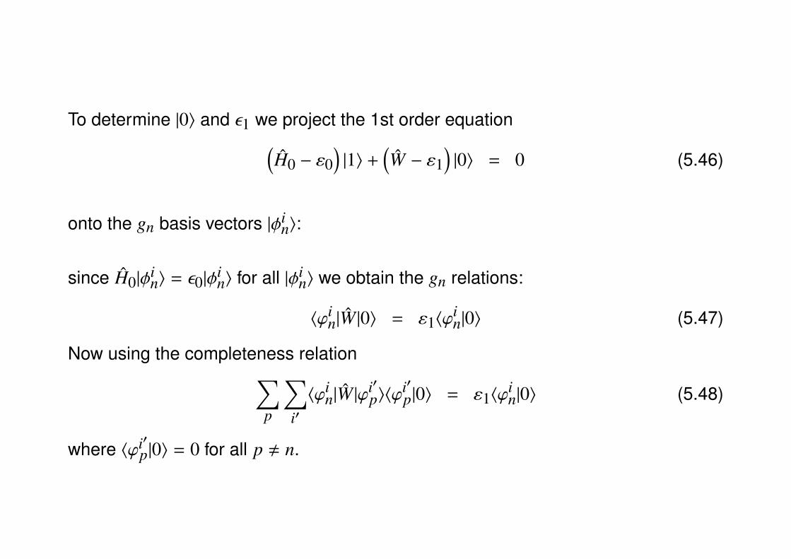
To determine |0〉 and ε1 we project the 1st order equation(H0 − ε0

)|1〉 +

(W − ε1

)|0〉 = 0 (5.46)

onto the gn basis vectors |φin〉:

since H0|φin〉 = ε0|φ

in〉 for all |φi

n〉 we obtain the gn relations:

〈ϕin|W |0〉 = ε1〈ϕ

in|0〉 (5.47)

Now using the completeness relation∑p

∑i′〈ϕi

n|W |ϕi′p〉〈ϕ

i′p|0〉 = ε1〈ϕ

in|0〉 (5.48)

where 〈ϕi′p|0〉 = 0 for all p , n.

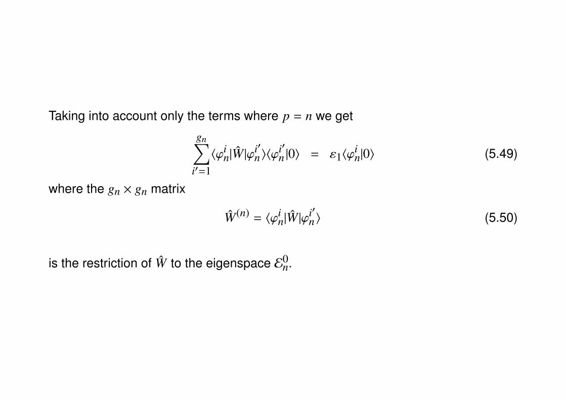
Taking into account only the terms where p = n we get

gn∑i′=1〈ϕi

n|W |ϕi′n〉〈ϕ

i′n |0〉 = ε1〈ϕ

in|0〉 (5.49)

where the gn × gn matrix

W(n) = 〈ϕin|W |ϕ

i′n〉 (5.50)

is the restriction of W to the eigenspace E0n.

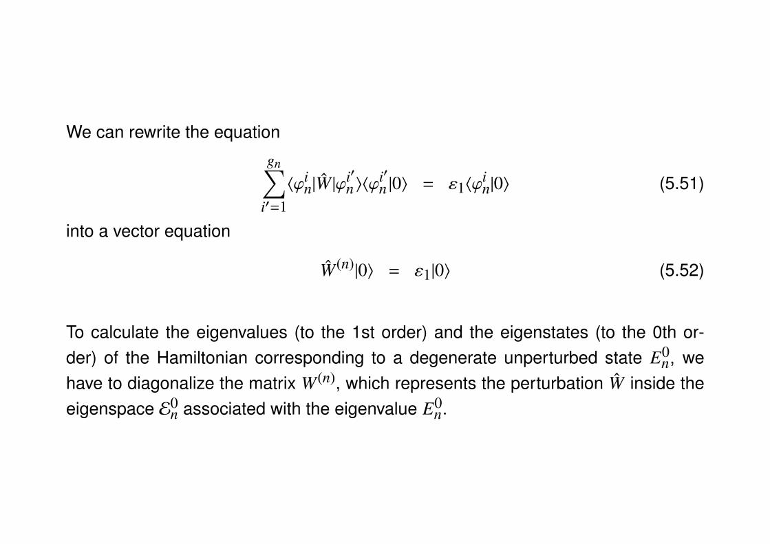
We can rewrite the equation

gn∑i′=1〈ϕi

n|W |ϕi′n〉〈ϕ

i′n |0〉 = ε1〈ϕ

in|0〉 (5.51)

into a vector equation

W(n)|0〉 = ε1|0〉 (5.52)

To calculate the eigenvalues (to the 1st order) and the eigenstates (to the 0th or-der) of the Hamiltonian corresponding to a degenerate unperturbed state E0

n, wehave to diagonalize the matrix W(n), which represents the perturbation W inside theeigenspace E0

n associated with the eigenvalue E0n.

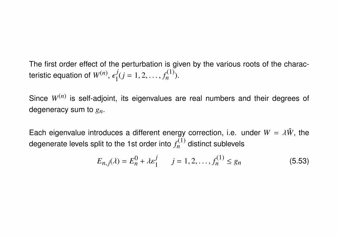
The first order effect of the perturbation is given by the various roots of the charac-teristic equation of W(n), ε j

1( j = 1, 2, . . . , f (1)n ).

Since W(n) is self-adjoint, its eigenvalues are real numbers and their degrees ofdegeneracy sum to gn.

Each eigenvalue introduces a different energy correction, i.e. under W = λW, thedegenerate levels split to the 1st order into f (1)

n distinct sublevels

En, j(λ) = E0n + λε

j1 j = 1, 2, . . . , f (1)

n ≤ gn (5.53)

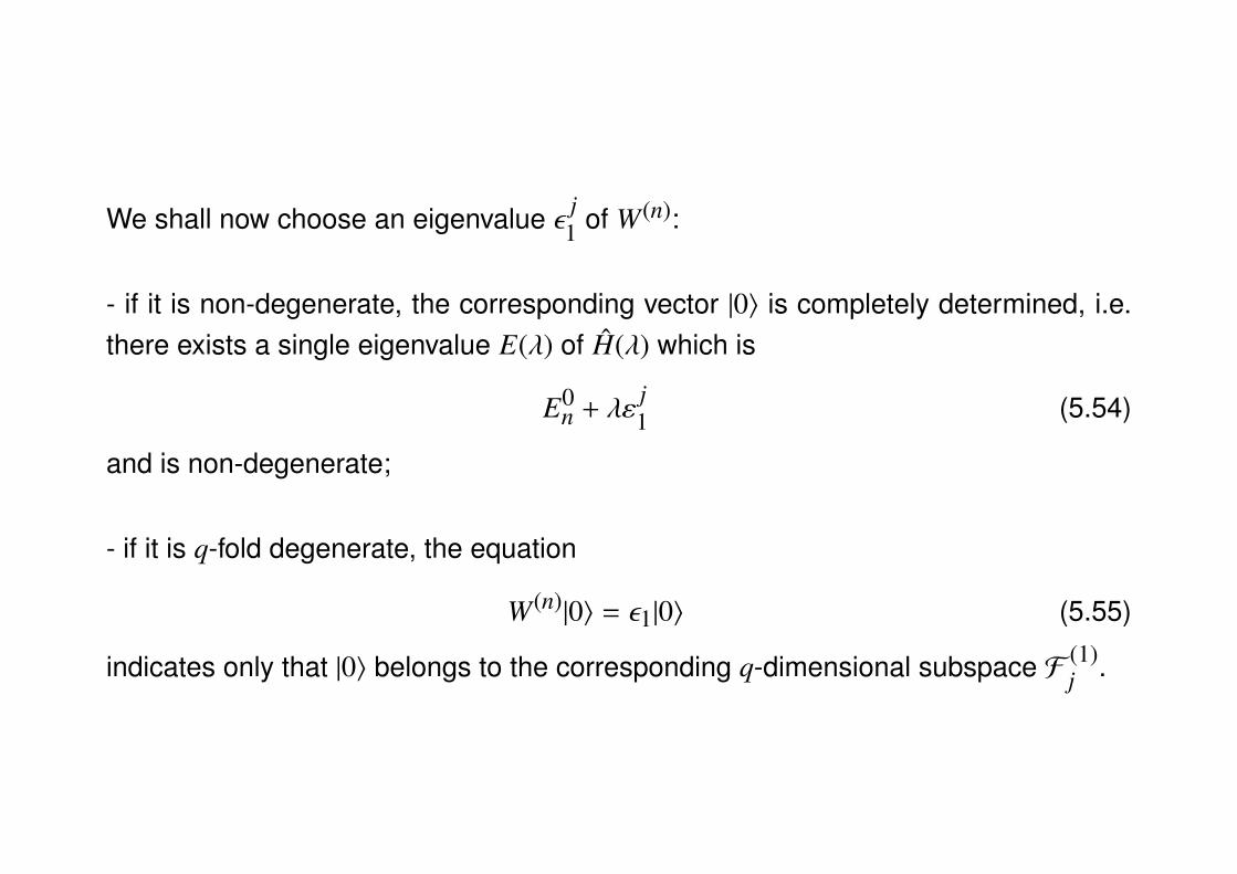
We shall now choose an eigenvalue ε j1 of W(n):

- if it is non-degenerate, the corresponding vector |0〉 is completely determined, i.e.there exists a single eigenvalue E(λ) of H(λ) which is

E0n + λε

j1 (5.54)

and is non-degenerate;

- if it is q-fold degenerate, the equation

W(n)|0〉 = ε1|0〉 (5.55)

indicates only that |0〉 belongs to the corresponding q-dimensional subspace F (1)j .