Embed Size (px)
Citation preview
APPROVED FOR PUBLIC RELEASE: DISTRIBUTION UNLIMITED
(25 November 1997)
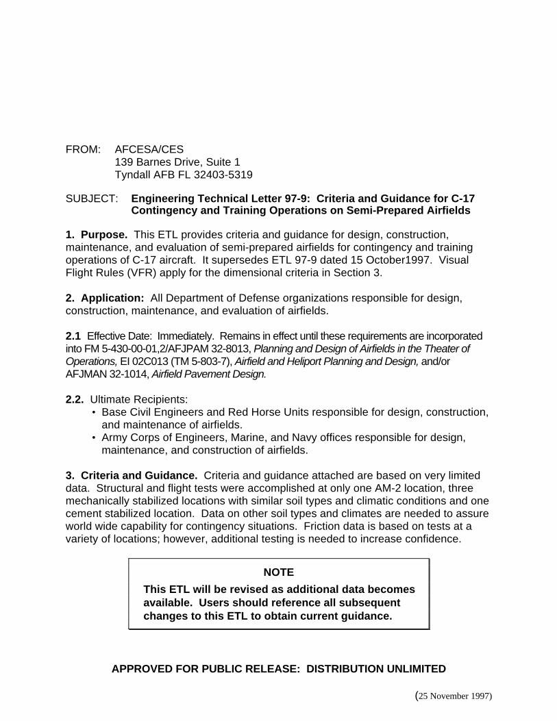
FROM: AFCESA/CES139 Barnes Drive, Suite 1Tyndall AFB FL 32403-5319
SUBJECT: Engineering Technical Letter 97-9: Criteria and Guidance for C-17Contingency and Training Operations on Semi-Prepared Airfields
1. Purpose. This ETL provides criteria and guidance for design, construction,maintenance, and evaluation of semi-prepared airfields for contingency and trainingoperations of C-17 aircraft. It supersedes ETL 97-9 dated 15 October1997. VisualFlight Rules (VFR) apply for the dimensional criteria in Section 3.
2. Application: All Department of Defense organizations responsible for design,construction, maintenance, and evaluation of airfields.
2.1 Effective Date: Immediately. Remains in effect until these requirements are incorporatedinto FM 5-430-00-01,2/AFJPAM 32-8013, Planning and Design of Airfields in the Theater ofOperations, EI 02C013 (TM 5-803-7), Airfield and Heliport Planning and Design, and/orAFJMAN 32-1014, Airfield Pavement Design.
2.2. Ultimate Recipients:• Base Civil Engineers and Red Horse Units responsible for design, construction,
and maintenance of airfields.• Army Corps of Engineers, Marine, and Navy offices responsible for design,
maintenance, and construction of airfields.
3. Criteria and Guidance. Criteria and guidance attached are based on very limiteddata. Structural and flight tests were accomplished at only one AM-2 location, threemechanically stabilized locations with similar soil types and climatic conditions and onecement stabilized location. Data on other soil types and climates are needed to assureworld wide capability for contingency situations. Friction data is based on tests at avariety of locations; however, additional testing is needed to increase confidence.
NOTE
This ETL will be revised as additional data becomesavailable. Users should reference all subsequentchanges to this ETL to obtain current guidance.
(25 November 1997)
4. Contacts. Mr. Jim Greene, DSN 523-6334, commercial (850)283-6334; or Mr. DickSmith, DSN 523-6084, commercial (850)283-6084.
William G. Schauz, Colonel, USAF 2 AtchDirector of Technical Support 1. Criteria for Design, Maintenance, and
Evaluation of Semi-Prepared Airfieldsfor Contingency Operations of the C-17Aircraft
2. Distribution List
Atch 1(1 of 162)
(25 November 1997)
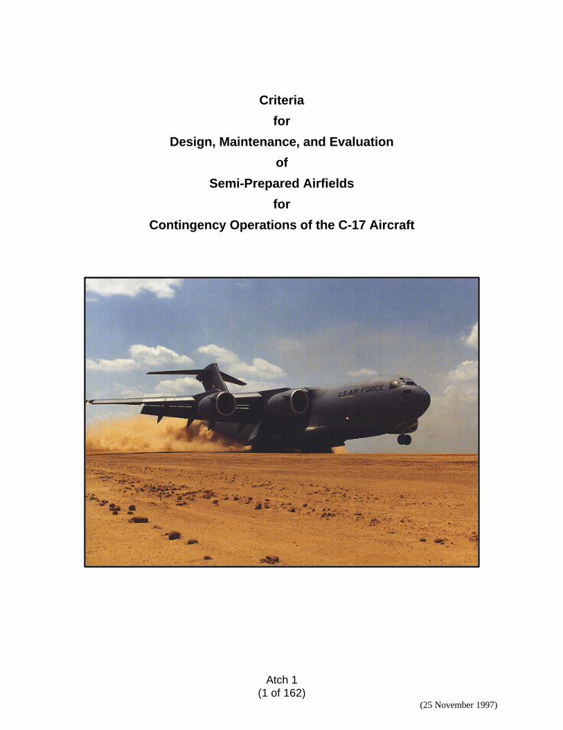
Criteria
for
Design, Maintenance, and Evaluation
of
Semi-Prepared Airfields
for
Contingency Operations of the C-17 Aircraft
Atch 1(2 of 162)
(25 November 1997)
Contents
Section
1 Introduction
2 Aircraft Characteristics
3 Dimensional Criteria
4 Structural Design Criteria
Appendixes
A Classification and Field Identification of Soils
B Condition Survey and Maintenance Procedures
C Structural Evaluation Procedures for Contingency Operations
D Friction Test Procedures for Contingency Operations
E Landing Zone Checklist

Atch 1(3 of 162)
(25 November 1997)
Section 1. Introduction
1.1. References:• FM 5-430-00-01, 02/ AFJPAM 32-8013, Volumes I and II, Planning and Design
of Roads, Airfields, and Heliports in the Theater of Operations• EI 02C013 (TM 5-803-7) / AFJMAN 32-1013, Airfield and Heliport Planning and
Design• Pavement-Transportation Computer Aided Structural Engineering (PCASE)
design and evaluation computer programs:− Dynamic Cone Penetrometer (DCP) program is used to plot DCP data and
establish soil layer thicknesses and strengths.− Unsurfaced Design (UNSURF) program is used to aid in design of semi-
prepared airfields.− Unsurfaced Evaluation (UNSEVA) program is used to determine aircraft
allowable gross weights and/or passes based upon layer structuresestablished with the DCP.
• Airfield Friction Meter MK2 Operating Instructions, Rev 3.1x, Issue 3, BowmonkLtd., Norwich, England, 1995
PCASE programs are available on the World Wide WEB (WWW) at http://pavement.wes.army.mil/pcase.html. For access, open a Uniform Resource Listing/Locator(URL) to the address, which will jump to the PCASE homepage for computer programaccess. For File Transfer Protocol (FTP) Anonymous Network Access, FTP to:pavement.wes.army.mil using 'anonymous' as the log in name, and 'pcase' as thepassword. Change directory to 'pub' (cd pub) and look at directory contents (ls).Change transfer type to binary (binary) and then use the 'get' command to retrieve anyfile you wish. For example, if you wish to get the file 'unsurf1_0.exe' then type 'getunsurf1_0.exe".
Note: All programs on the WWW homepage and FTP site are compressedexecutables. Upon first time execution of any program, multiple files will be extracted,therefore; it is vital that each program is put in its own subdirectory with no otherfiles when it is first executed.
1.2. Definitions.
1.2.1. Acronyms:• ACN – Aircraft Classification Number• CBR – California Bearing Ratio• DCP – Dynamic Cone Penetrometer• ETL – Engineering Technical Letter• FASSI – Frost Area Soil Support Index• FTP – File Transfer Protocol• HMMWV – High Mobility Multi-purpose Wheeled Vehicle
Atch 1(4 of 162)
(25 November 1997)
• PCASE – Pavement-Transportation Computer Aided Structural Design andEvaluation computer Programs
• PCN – Pavement Classification Number• RCR –Runway Condition Rating• RRM – Rolling Resistant Material• SPACI – Semi-prepared Airfield Condition Index• SST – Special Tactics Team• UNSEVA – Unsurfaced Evaluation Program• UNSURF – Unsurfaced Design Program• USCS – Unified Soil Classification System• VAMP – Visual Assault Zone Marker Panel• VFR – Visual Flight Rules
1.2.2. Terms:• Pass – The movement of an aircraft over a specific spot or location on a
pavement feature.• Base or Subbase Courses – Natural or processed materials placed on the
subgrade.• Subgrade – Natural in-place soil upon which a pavement, base, or subbase
course is constructed.• Compacted Subgrade – The upper part of the subgrade.
1.3. Airfield Types. The C-17 can operate on paved or semi-prepared airfields andmatting. Paved airfields consist of conventional rigid and flexible pavements and aregenerally used for routine operations. A “semi-prepared” airfield refers to an unpavedairfield. The amount of engineering effort required to develop a semi-prepared airfielddepends on the planned operation, the service life needed to support these operations,and the existing soil and weather conditions. Semi-prepared construction/maintenancepreparations may range from those sufficient for limited use to those required forcontinuous routine operations. Options for surface preparation may includestabilization, addition of an aggregate course, compaction of in-place soils, or matting.
1.4. Types of Operations. Three types of operations are anticipated with the C-17aircraft. Visual flight rules apply for contingency and training operations.
• Routine operations consist of normal day to day operations conducted on pavedsurfaces.
• Contingency operations are normally short term operations connected withconflicts or emergencies. Airfields for contingency operations can be paved orunpaved. Since operations are limited, structural requirements are not as great.In addition, higher risk to aircraft and personnel may be justified, sorequirements such as clearances, are not as stringent.
• Training operations involve training for contingency situations. They can beconducted on paved or unpaved runways (semi-prepared). Since trainingairfields are for long-term operations, semi-prepared surface structural and
Atch 1(5 of 162)
(25 November 1997)
dimensional requirements are more stringent than for contingency airfields.Stabilization may be required.
1.5. Purpose. The purpose of this document is to provide criteria and guidance toDoD organizations concerned with planning, design, construction, evaluation andmaintenance of semi-prepared airfields for contingency and training operations of theC-17. This document will remain in effect until the criteria and data are incorporatedinto FM 5-430-00-01.02/AFJPAM 32-8013, Volumes I and II, Planning and Design ofRoads, Airfields, and Heliports in the Theater of Operations. Criteria for planning anddesign of airfields for C-17 routine and training operations will be contained in EI02C013 / AFJMAN 32-1013.
Atch 1(6 of 162)
(25 November 1997)
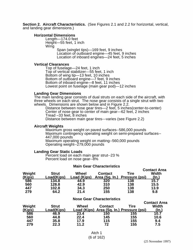
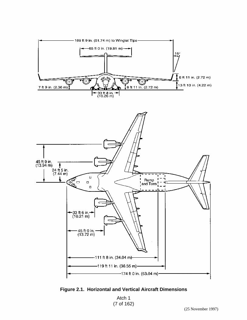
Section 2. Aircraft Characteristics. (See Figures 2.1 and 2.2 for horizontal, vertical,and landing gear dimensions.)
Horizontal DimensionsLength—174.0 feetHeight—55 feet, 1 inchWing
Span (winglet tips)—169 feet, 9 inchesLocation of outboard engine—45 feet, 9 inchesLocation of inboard engines—24 feet, 5 inches
Vertical ClearancesTop of fuselage—24 feet, 1 inchTop of vertical stabilizer—55 feet, 1 inchBottom of wing tip—13 feet, 10 inchesBottom of outboard engine—7 feet, 9 inchesBottom of inboard engine—8 feet, 11 inchesLowest point on fuselage (main gear pod)—12 inches
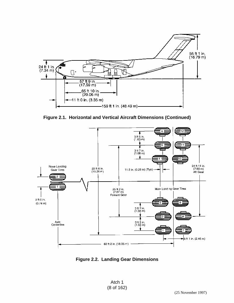
Landing Gear DimensionsThe main landing gear consists of dual struts on each side of the aircraft, withthree wheels on each strut. The nose gear consists of a single strut with twowheels. Dimensions are shown below and in Figure 2.2.
Distance between nose gear tires—2 feet, 5 inches(center-to-center)Center of nose gear to center of main gear—62 feet, 2 inchesTread –33 feet, 8 inchesDistance between main gear tires---varies (see Figure 2.2)
Aircraft WeightsMaximum gross weight on paved surfaces--586,000 poundsMaximum contingency operating weight on semi-prepared surfaces--447,000 poundsMaximum operating weight on matting--560,000 poundsOperating weight--279,000 pounds
Landing Gear Static LoadsPercent load on each main gear strut--23 %Percent load on nose gear--8%
Main Gear Characteristics Contact Area
Weight Strut Wheel Contact Tire Width(Kips) Load(Kips) Load (Kips) Area (Sq. In.) Pressure (psi) (In.)
586 134.8 44.9 320 138 15.7560 128.8 42.9 310 138 15.5447 102.8 34.3 250 138 13.9279 64.2 21.4 155 138 9.8
Nose Gear Characteristics Contact Area
Weight Strut Wheel Contact Tire Width(Kips) Load(Kips) Load (Kips) Area (Sq. In.) Pressure (psi) (In.)
586 46.9 23.4 150 155 10.7560 44.8 22.4 145 155 10.6447 35.8 17.9 115 155 9.4279 22.3 11.2 72 155 7.5
Atch 1(7 of 162)
(25 November 1997)
Figure 2.1. Horizontal and Vertical Aircraft Dimensions
Atch 1(8 of 162)
(25 November 1997)
Figure 2.1. Horizontal and Vertical Aircraft Dimensions (Continued)
Figure 2.2. Landing Gear Dimensions
Atch 1(9 of 162)
(25 November 1997)
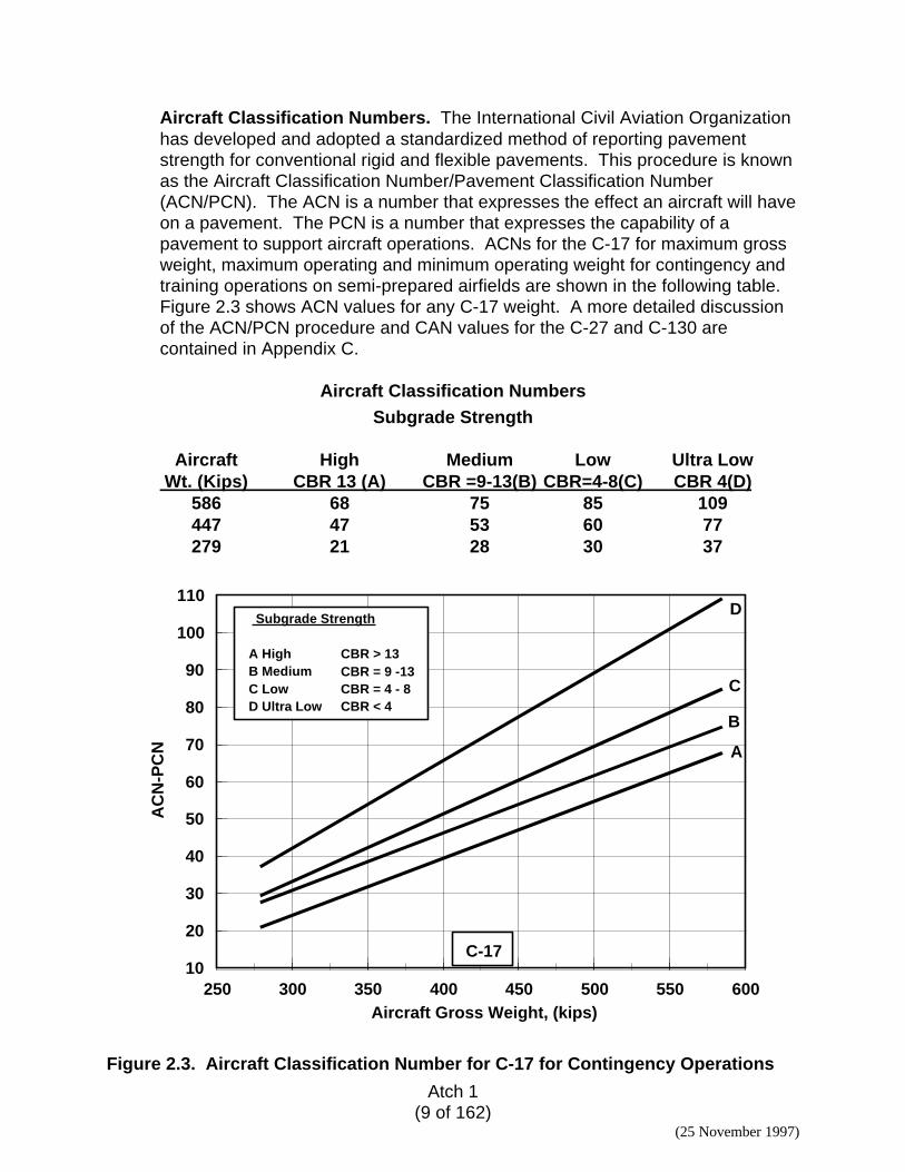
Aircraft Classification Numbers. The International Civil Aviation Organizationhas developed and adopted a standardized method of reporting pavementstrength for conventional rigid and flexible pavements. This procedure is knownas the Aircraft Classification Number/Pavement Classification Number(ACN/PCN). The ACN is a number that expresses the effect an aircraft will haveon a pavement. The PCN is a number that expresses the capability of apavement to support aircraft operations. ACNs for the C-17 for maximum grossweight, maximum operating and minimum operating weight for contingency andtraining operations on semi-prepared airfields are shown in the following table.Figure 2.3 shows ACN values for any C-17 weight. A more detailed discussionof the ACN/PCN procedure and CAN values for the C-27 and C-130 arecontained in Appendix C.
Aircraft Classification NumbersSubgrade Strength
Aircraft High Medium Low Ultra Low Wt. (Kips) CBR 13 (A) CBR =9-13(B) CBR=4-8(C) CBR 4(D)
586 68 75 85 109447 47 53 60 77279 21 28 30 37
250 300 350 400 450 500 550 600Aircraft Gross Weight, (kips)
10
20
30
40
50
60
70
80
90
100
110
AC
N-P
CN A
C-17
B
C
D Subgrade Strength
A High B Medium C Low D Ultra Low
CBR > 13CBR = 9 -13 CBR = 4 - 8 CBR < 4
Figure 2.3. Aircraft Classification Number for C-17 for Contingency Operations
Atch 1(10 of 162)
(25 November 1997)
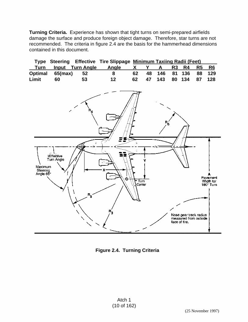
Turning Criteria. Experience has shown that tight turns on semi-prepared airfieldsdamage the surface and produce foreign object damage. Therefore, star turns are notrecommended. The criteria in figure 2.4 are the basis for the hammerhead dimensionscontained in this document.
Type Steering Effective Tire Slippage Minimum Taxiing Radii (Feet) Turn Input Turn Angle Angle X Y A R3 R4 R5 R6Optimal 65(max) 52 8 62 48 146 81 136 88 129Limit 60 53 12 62 47 143 80 134 87 128
Figure 2.4. Turning Criteria
Atch 1(11 of 162)
(25 November 1997)
Section 3. Dimensional Criteria
3.1. Contents. This section presents design considerations unique for C-17contingency airfields. This criteria is given as a supplement to the criteria given inAFJPAM 32-8013/FM 5-430-00-2, Planning and Design of Roads, Airfields andHeliports. With introduction of the C-17 came the requirement to validate existingdesign criteria or develop new criteria as required to accommodate contingencyoperations on semi-prepared runway surfaces.
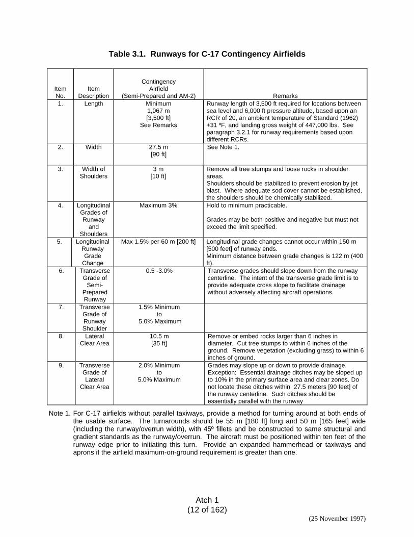
3.2. Runway and Overrun Descriptions. Tables 3.1 and 3.2 provide dimensionalcriteria for layout and design of assault landing zones.
3.2.1. Length. For a semi-prepared runway located between sea level and 6,000 feetpressure altitude, the minimum length requirement for C-17 operations is 3,500 feetwith 300-foot overruns on each end. This length requirement, based upon an RCR of20, assumes an ambient temperature equal Standard (1962) plus 31 ºF, and a landinggross weight of 447,000 pounds. Based upon these same temperature and weightassumptions, the runway length will vary with different RCRs as follows:
Note: The runway lengths do not include under/overruns.
3.2.2. Width. The widths of these landing surfaces must be sufficient to protect theaircraft landing gear and the engines. Table 3.1 provides the minimum runway width.
3.2.3. Longitudinal Gradients of Operational Surfaces. Gradient constraints are basedupon reverse aircraft operations conducted on hard surfaces. Caution should be usedwhen backing aircraft on soft soil conditions, at any gradient.
3.2.4. Shoulders. Shoulders are graded and cleared of obstacles and slope downwardaway from the runway where practical to facilitate drainage.
RCRPressure Altitude
(feet)Runway Length
(feet)
20 0 -6,000 3,500
16 0 - 2,000 3,5002,001 - 5,000 4,0005,001 - 6,000 4,500
12 0 - 2,000 4,0002,001 - 5,000 4,5005,001 - 6,000 5,000
8 0 - 3,000 5,000
4
3,001 - 5,0005,001 - 6,000
0 - 2,0002,001 - 4,0004,001 - 6,000
5,5006,0006,0006,5007,000
Atch 1(12 of 162)
(25 November 1997)
Table 3.1. Runways for C-17 Contingency Airfields
ItemNo.
ItemDescription
ContingencyAirfield
(Semi-Prepared and AM-2) Remarks1. Length Minimum
1,067 m[3,500 ft]
See Remarks
Runway length of 3,500 ft required for locations betweensea level and 6,000 ft pressure altitude, based upon anRCR of 20, an ambient temperature of Standard (1962)+31 ºF, and landing gross weight of 447,000 lbs. Seeparagraph 3.2.1 for runway requirements based upondifferent RCRs.
2. Width 27.5 m[90 ft]
See Note 1.
3. Width ofShoulders
3 m[10 ft]
Remove all tree stumps and loose rocks in shoulderareas.Shoulders should be stabilized to prevent erosion by jetblast. Where adequate sod cover cannot be established,the shoulders should be chemically stabilized.
4. LongitudinalGrades ofRunway
andShoulders
Maximum 3% Hold to minimum practicable.
Grades may be both positive and negative but must notexceed the limit specified.
5. LongitudinalRunwayGrade
Change
Max 1.5% per 60 m [200 ft] Longitudinal grade changes cannot occur within 150 m[500 feet] of runway ends.Minimum distance between grade changes is 122 m (400ft).
6. TransverseGrade of
Semi-PreparedRunway
0.5 -3.0% Transverse grades should slope down from the runwaycenterline. The intent of the transverse grade limit is toprovide adequate cross slope to facilitate drainagewithout adversely affecting aircraft operations.
7. TransverseGrade ofRunwayShoulder
1.5% Minimumto
5.0% Maximum
8. LateralClear Area
10.5 m[35 ft]
Remove or embed rocks larger than 6 inches indiameter. Cut tree stumps to within 6 inches of theground. Remove vegetation (excluding grass) to within 6inches of ground.
9. TransverseGrade ofLateral
Clear Area
2.0% Minimumto
5.0% Maximum
Grades may slope up or down to provide drainage.Exception: Essential drainage ditches may be sloped upto 10% in the primary surface area and clear zones. Donot locate these ditches within 27.5 meters [90 feet] ofthe runway centerline. Such ditches should beessentially parallel with the runway
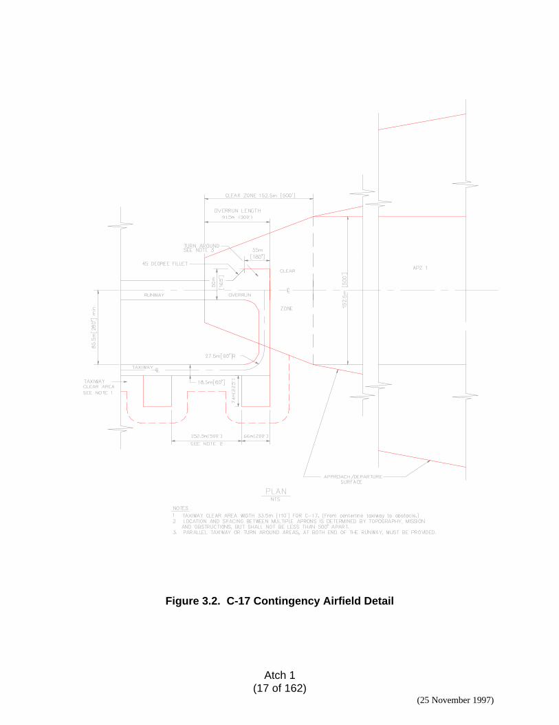
Note 1. For C-17 airfields without parallel taxiways, provide a method for turning around at both ends ofthe usable surface. The turnarounds should be 55 m [180 ft] long and 50 m [165 feet] wide(including the runway/overrun width), with 45º fillets and be constructed to same structural andgradient standards as the runway/overrun. The aircraft must be positioned within ten feet of therunway edge prior to initiating this turn. Provide an expanded hammerhead or taxiways andaprons if the airfield maximum-on-ground requirement is greater than one.
Atch 1(13 of 162)
(25 November 1997)
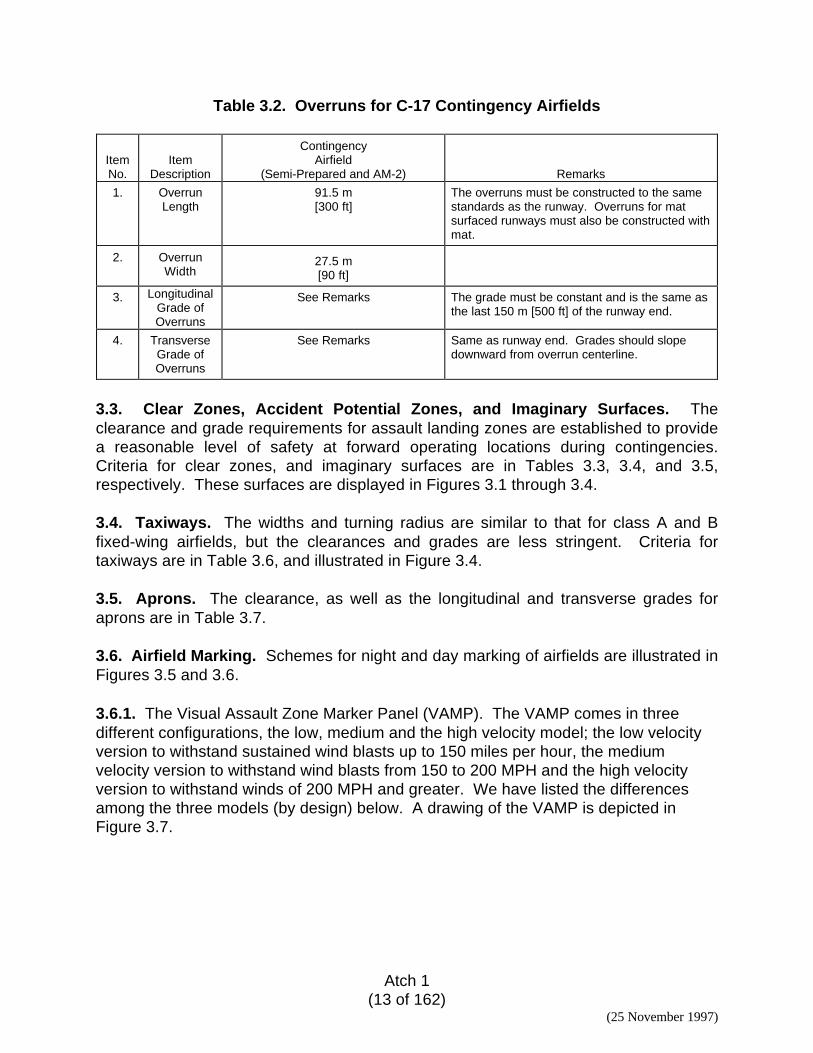
Table 3.2. Overruns for C-17 Contingency Airfields
ItemNo.
ItemDescription
ContingencyAirfield
(Semi-Prepared and AM-2) Remarks
1. OverrunLength
91.5 m[300 ft]
The overruns must be constructed to the samestandards as the runway. Overruns for matsurfaced runways must also be constructed withmat.
2. OverrunWidth
27.5 m[90 ft]
3. LongitudinalGrade ofOverruns
See Remarks The grade must be constant and is the same asthe last 150 m [500 ft] of the runway end.
4. TransverseGrade ofOverruns
See Remarks Same as runway end. Grades should slopedownward from overrun centerline.
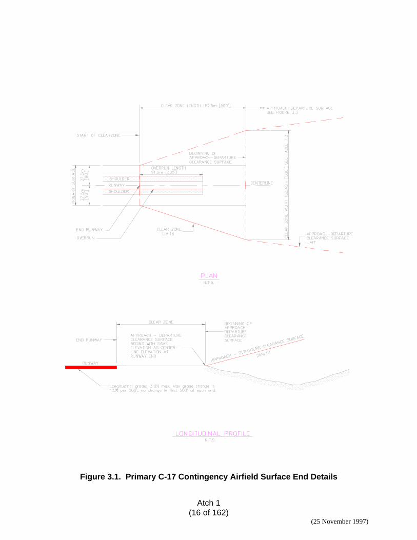
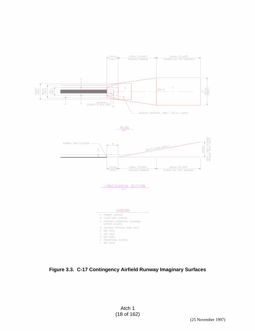
3.3. Clear Zones, Accident Potential Zones, and Imaginary Surfaces. Theclearance and grade requirements for assault landing zones are established to providea reasonable level of safety at forward operating locations during contingencies.Criteria for clear zones, and imaginary surfaces are in Tables 3.3, 3.4, and 3.5,respectively. These surfaces are displayed in Figures 3.1 through 3.4.
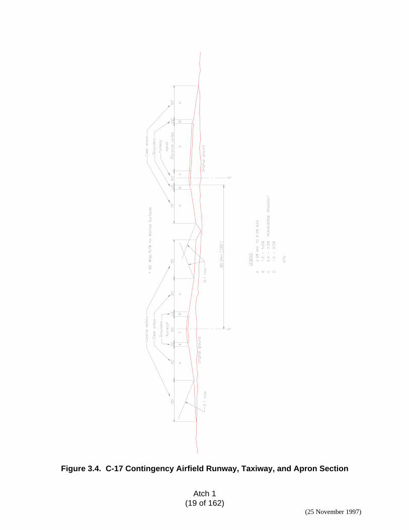
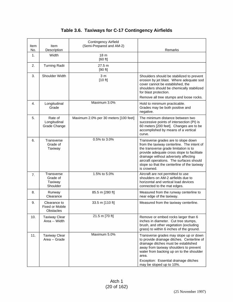
3.4. Taxiways. The widths and turning radius are similar to that for class A and Bfixed-wing airfields, but the clearances and grades are less stringent. Criteria fortaxiways are in Table 3.6, and illustrated in Figure 3.4.
3.5. Aprons. The clearance, as well as the longitudinal and transverse grades foraprons are in Table 3.7.
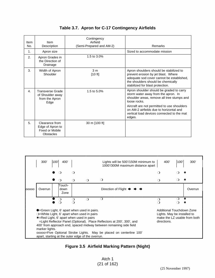
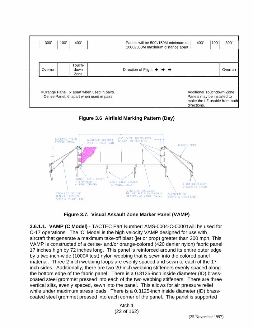
3.6. Airfield Marking. Schemes for night and day marking of airfields are illustrated inFigures 3.5 and 3.6.
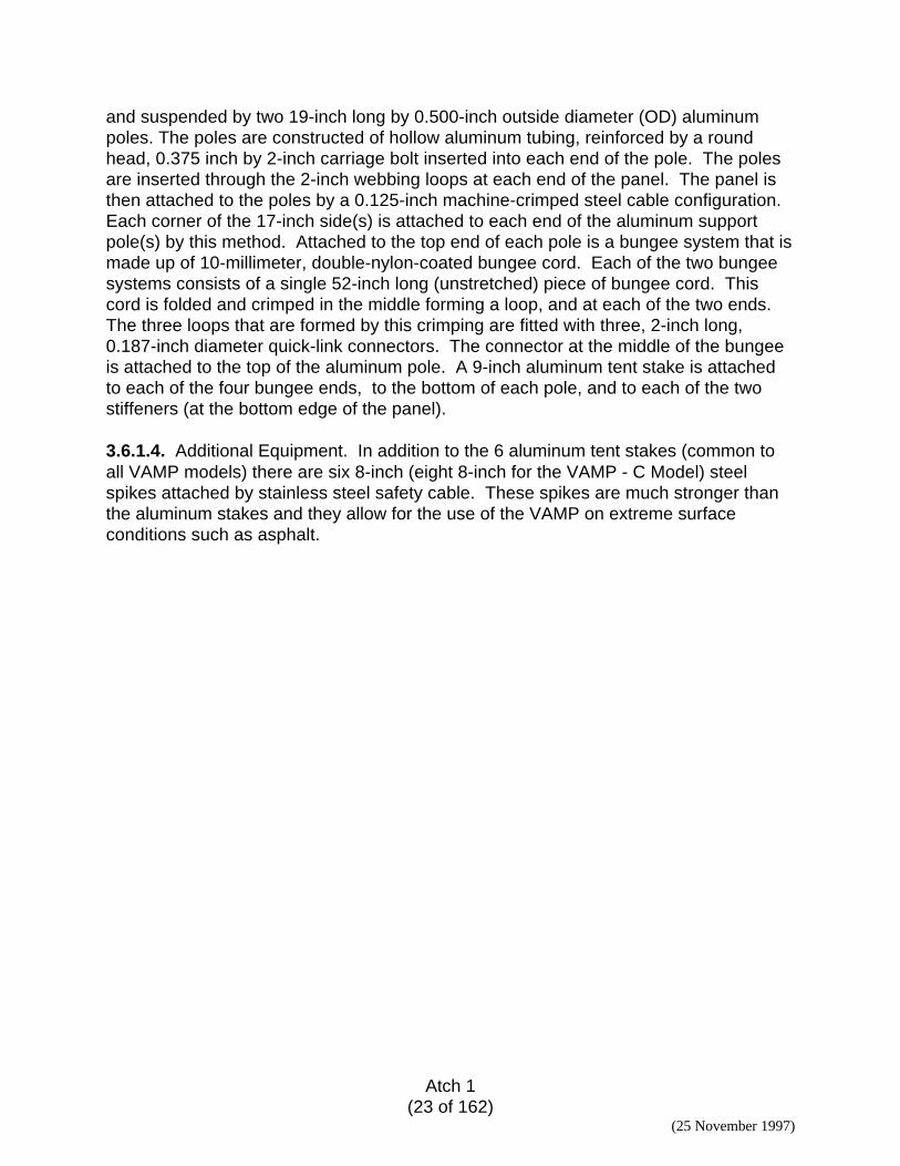
3.6.1. The Visual Assault Zone Marker Panel (VAMP). The VAMP comes in threedifferent configurations, the low, medium and the high velocity model; the low velocityversion to withstand sustained wind blasts up to 150 miles per hour, the mediumvelocity version to withstand wind blasts from 150 to 200 MPH and the high velocityversion to withstand winds of 200 MPH and greater. We have listed the differencesamong the three models (by design) below. A drawing of the VAMP is depicted inFigure 3.7.
Atch 1(14 of 162)
(25 November 1997)
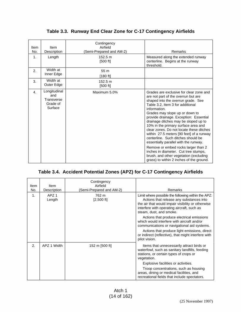
Table 3.3. Runway End Clear Zone for C-17 Contingency Airfields
ItemNo.
ItemDescription
ContingencyAirfield
(Semi-Prepared and AM-2) Remarks
1. Length 152.5 m[500 ft]
Measured along the extended runwaycenterline. Begins at the runwaythreshold.
2. Width atInner Edge
55 m
[180 ft]
3. Width atOuter Edge
152.5 m[500 ft]
4. Longitudinaland
TransverseGrade ofSurface
Maximum 5.0% Grades are exclusive for clear zone andare not part of the overrun but areshaped into the overrun grade. SeeTable 3.2, Item 3 for additionalinformation.Grades may slope up or down toprovide drainage. Exception: Essentialdrainage ditches may be sloped up to10% in the primary surface area andclear zones. Do not locate these ditcheswithin 27.5 meters [90 feet] of a runwaycenterline. Such ditches should beessentially parallel with the runway.
Remove or embed rocks larger than 2inches in diameter. Cut tree stumps,brush, and other vegetation (excludinggrass) to within 2 inches of the ground.
Table 3.4. Accident Potential Zones (APZ) for C-17 Contingency Airfields
ItemNo.
ItemDescription
ContingencyAirfield
(Semi-Prepared and AM-2) Remarks
1. APZ 1Length
762 m[2,500 ft]
Limit where possible the following within the APZ:Actions that release any substances into
the air that would impair visibility or otherwiseinterfere with operating aircraft, such assteam, dust, and smoke.
Actions that produce electrical emissionswhich would interfere with aircraft and/orcommunications or navigational aid systems.
Actions that produce light emissions, director indirect (reflective), that might interfere withpilot vision.
2. APZ 1 Width 152 m [500 ft] Items that unnecessarily attract birds orwaterfowl, such as sanitary landfills, feedingstations, or certain types of crops orvegetation.
Explosive facilities or activities.
Troop concentrations, such as housingareas, dining or medical facilities, andrecreational fields that include spectators.
Atch 1(15 of 162)
(25 November 1997)
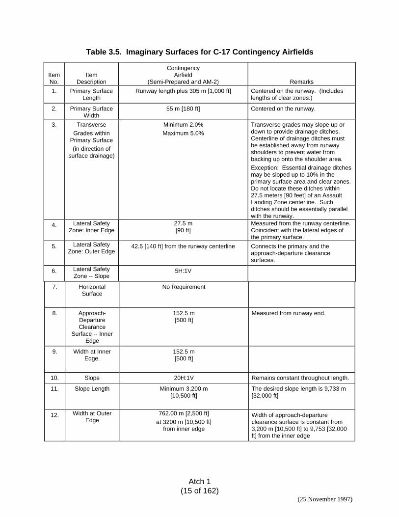
Table 3.5. Imaginary Surfaces for C-17 Contingency Airfields
ItemNo.
ItemDescription
ContingencyAirfield
(Semi-Prepared and AM-2) Remarks
1. Primary SurfaceLength
Runway length plus 305 m [1,000 ft] Centered on the runway. (Includeslengths of clear zones.)
2. Primary SurfaceWidth
55 m [180 ft] Centered on the runway.
3. Transverse
Grades withinPrimary Surface
(in direction ofsurface drainage)
Minimum 2.0%
Maximum 5.0%
Transverse grades may slope up ordown to provide drainage ditches.Centerline of drainage ditches mustbe established away from runwayshoulders to prevent water frombacking up onto the shoulder area.
Exception: Essential drainage ditchesmay be sloped up to 10% in theprimary surface area and clear zones.Do not locate these ditches within27.5 meters [90 feet] of an AssaultLanding Zone centerline. Suchditches should be essentially parallelwith the runway.
4. Lateral SafetyZone: Inner Edge
27.5 m[90 ft]
Measured from the runway centerline.Coincident with the lateral edges ofthe primary surface.
5. Lateral SafetyZone: Outer Edge
42.5 [140 ft] from the runway centerline Connects the primary and theapproach-departure clearancesurfaces.
6. Lateral SafetyZone -- Slope
5H:1V
7. HorizontalSurface
No Requirement
8. Approach-DepartureClearance
Surface -- InnerEdge
152.5 m[500 ft]
Measured from runway end.
9. Width at InnerEdge.
152.5 m[500 ft]
10. Slope 20H:1V Remains constant throughout length.
11. Slope Length Minimum 3,200 m[10,500 ft]
The desired slope length is 9,733 m[32,000 ft]
12. Width at OuterEdge
762.00 m [2,500 ft]
at 3200 m [10,500 ft]from inner edge
Width of approach-departureclearance surface is constant from3,200 m [10,500 ft] to 9,753 [32,000ft] from the inner edge
Atch 1(16 of 162)
(25 November 1997)
Figure 3.1. Primary C-17 Contingency Airfield Surface End Details
Atch 1(17 of 162)
(25 November 1997)
Figure 3.2. C-17 Contingency Airfield Detail
Atch 1(18 of 162)
(25 November 1997)
Figure 3.3. C-17 Contingency Airfield Runway Imaginary Surfaces
Atch 1(19 of 162)
(25 November 1997)
Figure 3.4. C-17 Contingency Airfield Runway, Taxiway, and Apron Section
Atch 1(20 of 162)
(25 November 1997)
Table 3.6. Taxiways for C-17 Contingency Airfields
ItemNo.
ItemDescription
Contingency Airfield(Semi-Prepared and AM-2)
Remarks
1. Width 18 m[60 ft]
2. Turning Radii 27.5 m[90 ft]
3. Shoulder Width 3 m[10 ft]
Shoulders should be stabilized to preventerosion by jet blast. Where adequate sodcover cannot be established, theshoulders should be chemically stabilizedfor blast protection.
Remove all tree stumps and loose rocks.
4. LongitudinalGrade
Maximum 3.0% Hold to minimum practicable.Grades may be both positive andnegative.
5. Rate ofLongitudinal
Grade Change
Maximum 2.0% per 30 meters [100 feet] The minimum distance between twosuccessive points of intersection (PI) is60 meters [200 feet]. Changes are to beaccomplished by means of a verticalcurve.
6. TransverseGrade ofTaxiway
0.5% to 3.0% Transverse grades are to slope downfrom the taxiway centerline. The intent ofthe transverse grade limitation is toprovide adequate cross slope to facilitatedrainage without adversely affectingaircraft operations. The surfaces shouldslope so that the centerline of the taxiwayis crowned.
7. TransverseGrade ofTaxiwayShoulder
1.5% to 5.0% Aircraft are not permitted to useshoulders on AM-2 airfields due tohorizontal and vertical load devicesconnected to the mat edges.
8. RunwayClearance
85.5 m [280 ft] Measured from the runway centerline tonear edge of the taxiway.
9. Clearance toFixed or Mobile
Obstacles
33.5 m [110 ft] Measured from the taxiway centerline.
10. Taxiway ClearArea -- Width
21.5 m [70 ft] Remove or embed rocks larger than 6inches in diameter. Cut tree stumps,brush, and other vegetation (excludinggrass) to within 6 inches of the ground.
11. Taxiway ClearArea -- Grade
Maximum 5.0% Transverse grades may slope up or downto provide drainage ditches. Centerline ofdrainage ditches must be establishedaway from taxiway shoulders to preventwater from backing up on to the shoulderarea.
Exception: Essential drainage ditchesmay be sloped up to 10%.
Atch 1(21 of 162)
(25 November 1997)
Table 3.7. Apron for C-17 Contingency Airfields
ItemNo.
ItemDescription
ContingencyAirfield
(Semi-Prepared and AM-2) Remarks
1. Apron size Sized to accommodate mission
2. Apron Grades inthe Direction of
Drainage
1.5 to 3.0%
3. Width of ApronShoulder
3 m[10 ft]
Apron shoulders should be stabilized toprevent erosion by jet blast. Whereadequate sod cover cannot be established,the shoulders should be chemicallystabilized for blast protection.
4. Transverse Gradeof Shoulder awayfrom the Apron
Edge
1.5 to 5.0% Apron shoulder should be graded to carrystorm water away from the apron. Inshoulder areas, remove all tree stumps andloose rocks.
Aircraft are not permitted to use shoulderson AM-2 airfields due to horizontal andvertical load devices connected to the matedges.
5. Clearance fromEdge of Apron toFixed or Mobile
Obstacles
30 m [100 ft]
300’ 100’ 400’ Lights will be 500’/150M minimum to1000’/300M maximum distance apart
400’ 100’ 300’
l m m m m Y
l m••• m • m • m m • m Y
Touch-ooooo Overrun down Direction of Flight è è è Overrun
Zone
l m••• m • m • m m • m Yl m m m m Y
l=Green Light, 6’ apart when used in pairs.m=White Light, 6’ apart when used in pairsY=Red Light, 6’ apart when used in pairs•=Light Reflector Panel (Optional). Place Reflectors at 200’, 300’, and400’ from approach end, spaced midway between remaining side fieldmarker lights.ooooo=Five Optional Strobe Lights. May be placed on centerline 100’apart, starting at the outer edge of the overrun.
Additional Touchdown ZoneLights. May be installed tomake the LZ usable from bothdirections.
Figure 3.5 Airfield Marking Pattern (Night)
Atch 1(22 of 162)
(25 November 1997)
300’ 100’ 400’ Panels will be 500’/150M minimum to1000’/300M maximum distance apart
400’ 100’ 300’
æ � � � � �æ � � � � � � �
Touch-Overrun down Direction of Flight è è è Overrun
Zoneæ � � � � � � �æ � � � � �
æ=Orange Panel, 6’ apart when used in pairs.� =Cerise Panel, 6’ apart when used in pairs
Additional Touchdown ZonePanels may be installed tomake the LZ usable from bothdirections.
Figure 3.6 Airfield Marking Pattern (Day)
Figure 3.7. Visual Assault Zone Marker Panel (VAMP)
3.6.1.1. VAMP (C Model) - TACTEC Part Number: AMS-0004-C-00001will be used forC-17 operations. The ‘C’ Model is the high velocity VAMP designed for use withaircraft that generate a maximum take-off blast (jet or prop) greater than 200 mph. ThisVAMP is constructed of a cerise- and/or orange-colored (420 denier nylon) fabric panel17 inches high by 72 inches long. This panel is reinforced around its entire outer edgeby a two-inch-wide (1000# test) nylon webbing that is sewn into the colored panelmaterial. Three 2-inch webbing loops are evenly spaced and sewn to each of the 17-inch sides. Additionally, there are two 20-inch webbing stiffeners evenly spaced alongthe bottom edge of the fabric panel. There is a 0.3125-inch inside diameter (ID) brass-coated steel grommet pressed into each of the two webbing stiffeners. There are threevertical slits, evenly spaced, sewn into the panel. This allows for air pressure reliefwhile under maximum stress loads. There is a 0.3125-inch inside diameter (ID) brass-coated steel grommet pressed into each corner of the panel. The panel is supported
Atch 1(23 of 162)
(25 November 1997)
and suspended by two 19-inch long by 0.500-inch outside diameter (OD) aluminumpoles. The poles are constructed of hollow aluminum tubing, reinforced by a roundhead, 0.375 inch by 2-inch carriage bolt inserted into each end of the pole. The polesare inserted through the 2-inch webbing loops at each end of the panel. The panel isthen attached to the poles by a 0.125-inch machine-crimped steel cable configuration.Each corner of the 17-inch side(s) is attached to each end of the aluminum supportpole(s) by this method. Attached to the top end of each pole is a bungee system that ismade up of 10-millimeter, double-nylon-coated bungee cord. Each of the two bungeesystems consists of a single 52-inch long (unstretched) piece of bungee cord. Thiscord is folded and crimped in the middle forming a loop, and at each of the two ends.The three loops that are formed by this crimping are fitted with three, 2-inch long,0.187-inch diameter quick-link connectors. The connector at the middle of the bungeeis attached to the top of the aluminum pole. A 9-inch aluminum tent stake is attachedto each of the four bungee ends, to the bottom of each pole, and to each of the twostiffeners (at the bottom edge of the panel).
3.6.1.4. Additional Equipment. In addition to the 6 aluminum tent stakes (common toall VAMP models) there are six 8-inch (eight 8-inch for the VAMP - C Model) steelspikes attached by stainless steel safety cable. These spikes are much stronger thanthe aluminum stakes and they allow for the use of the VAMP on extreme surfaceconditions such as asphalt.
Atch 1(24 of 162)
(25 November 1997)
Section 4. Structural Design Criteria
4.1. Introduction. This section presents the procedures for the structural design ofsemi-prepared airfields for the C-17 aircraft. This criteria is submitted as a supplementto that given in AFJPAM 32-8013/FM 5-430-00-2, Planning and Design of Roads,Airfields, and Heliports in the Theater of Operations. The introduction of the C-17resulted in the requirement to validate existing design criteria or develop new criteriafor contingency operations on semi-prepared runways. Semi-prepared airfields includeunsurfaced, aggregate-surfaced, and matted airfields. The criteria presented providesguidance for designing unsurfaced, aggregate-surfaced, and AM-2 mat-surfacedairfields for the operation of the C-17 aircraft.
4.2. Site Investigation. The site investigation for input to the structural design of asemi-prepared airfield is required to determine the in-place material properties and theproperties of the materials that are available for use in constructing a contingencyairfield. If an existing airfield is to be used, the evaluation portion of this document(Appendix C)should be used for investigating the capability of the airfield to support C-17 aircraft operations. If an existing airfield is not capable of supporting operations ofthe C-17 aircraft, the airfield will need to be upgraded or repairs and maintenance willbe required periodically during the mission. If it is determined that an existing airfieldwill be upgraded, the design portion of this document should be used and the materialcharacteristics of the existing airfield and available materials for upgrading will berequired for input to the design procedure. Knowledge of the current field condition ata site to be used for a contingency airfield is important (FM 5-430-00-2/AFJPAM 32-8013, Vol II). A proper description of the field condition at a proposed site includes thefollowing elements:
• ground cover (vegetation).• natural slopes.• soil types (classification).• soil density.• moisture content.• soil consistency (soft or hard).• existing drainage.• natural soil strength (in terms of California Bearing Ratio).
The information listed above is needed to determine the construction effort required toprovide an airfield capable of supporting the design number of operations of the C-17aircraft.
4.3. Base, Subbase, and Subgrade. A semi-prepared pavement structure typicallyconsists of three layers, the existing subgrade, a subbase, and a base course. A semi-prepared airfield may or may not have a subbase or a base. If the existing material (thesubgrade) is determined to be capable of supporting aircraft operations, no subbase orbase will be required. A subbase may consist of subbase material and a selectmaterial if a select material is available and of better quality than the subgrade (see FM5-430-00-1/AFPAM 32-8013, Vol 1, Chapter 5). The subgrade, potential subbase and
Atch 1(25 of 162)
(25 November 1997)
potential base materials need to be identified according to the Unified SoilClassification System (USCS). The evaluation portion of this document details theUSCS and field procedures for identifying soils and categorizing them according to theUSCS.
4.4. Soil Strength. The strength of the existing soil and any layers that will beconstructed above it are important parameters that are input to the design procedure.For semi-prepared pavements, the parameter used for indicating the strength of thelayers is the California Bearing Ratio (CBR). The CBR is a measure of the shearingresistance or strength of the soil. The evaluation portion of this document discussesthe tools and procedures for quickly obtaining an estimate of the CBR of in-place soils.For soils or materials that are to be placed (i.e. excavated, hauled, placed andcompacted) it will be necessary to determine the CBR that will be obtainable. Amoisture-density relationship (proctor curve) with accompanying laboratory CBR valuesis preferred for determining the CBR obtainable in the field and for specifying moistureand density requirements during construction. The CBR value of a material to beplaced may be significantly different than the in-place CBR of the material. Some soilsloose strength with remolding (see Chap 8 FM 5-410). Other soils if properly placedcan achieve CBR values greater than existed naturally. This is accomplished bycompacting the soil at or near optimum moisture content with an appropriatecompactive effort to obtain near maximum density. If maximum density is not achieved,a reduction in available performance results with a reduction in the number of aircraftoperations the airfield can support before failure occurs. Appendix C providesinformation on ranges of CBR that can be expected for different soil types. Aconservative estimate of CBR based on the material type may be used for preliminarydesign. During construction, the actual CBR can be measured with the dynamic conepenetrometer (DCP), and the design of the semi-prepared pavement can be adjustedas necessary. It should be noted that the CBR may change with time as the materialbecomes saturated. Saturation of the material usually results in a reduction in theCBR, this fact should be accounted for in the design of the airfield. Soaked laboratoryCBR values provide a good indication of the reduction in the CBR that may beexpected. Otherwise, conservative values based on the material type and the CBRdetermined in the field should be used for design. The gradation portion of thisdocument also provides an indication of the CBR that may be expected for materialsmeeting gradation and compaction requirements.
4.5. Soil Behavior. Soil is compacted to improve its load-carrying capability (5-430-00-2/AFJPAM 32-8013, Vol II). The compaction of soil reduces its natural variabilityproviding a more uniform structure for operating aircraft. Compaction also reduces thesoils permeability and susceptibility to erosion. Stabilization of soils can be used toimprove the strength of the soil or to reduce the effects of plasticity and high liquidlimits. Stabilizing can also provide dustproofing and waterproofing. Stabilization isaddressed in Section 4.8 of this document.
4.6. Gradation Requirements. The recommended gradation requirements and designCBR values for the subbase and select material (FM 5-430-00-1/AFPAM 32-8013, Vol
Atch 1(26 of 162)
(25 November 1997)
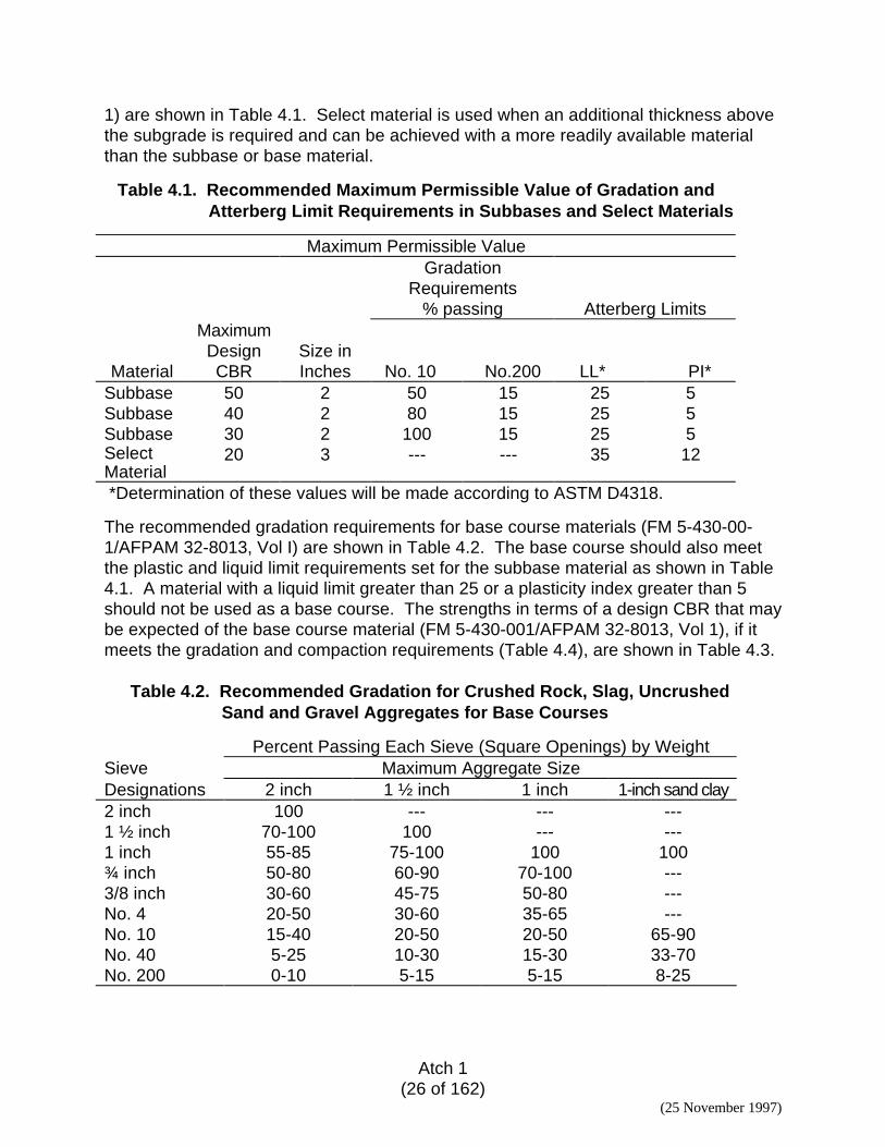
1) are shown in Table 4.1. Select material is used when an additional thickness abovethe subgrade is required and can be achieved with a more readily available materialthan the subbase or base material.
Table 4.1. Recommended Maximum Permissible Value of Gradation andAtterberg Limit Requirements in Subbases and Select Materials
Maximum Permissible ValueGradation
Requirements% passing Atterberg Limits
Material
MaximumDesignCBR
Size inInches No. 10 No.200 LL* PI*
Subbase 50 2 50 15 25 5Subbase 40 2 80 15 25 5Subbase 30 2 100 15 25 5SelectMaterial
20 3 --- --- 35 12
*Determination of these values will be made according to ASTM D4318.
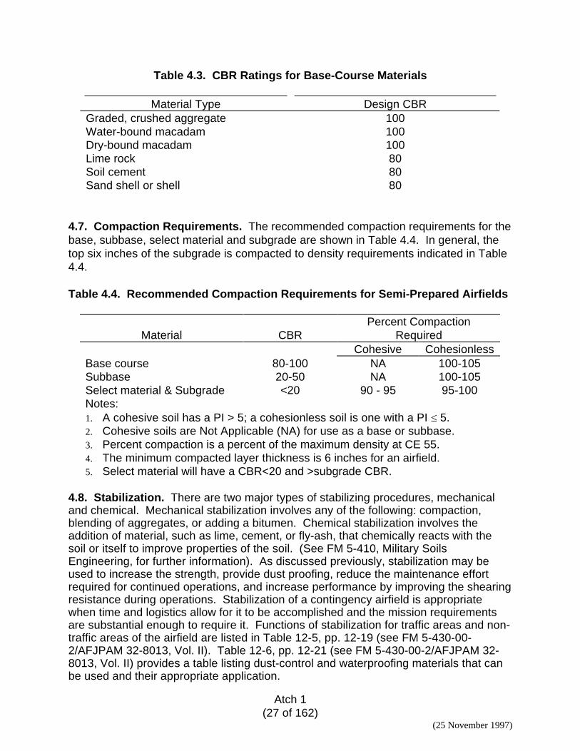
The recommended gradation requirements for base course materials (FM 5-430-00-1/AFPAM 32-8013, Vol I) are shown in Table 4.2. The base course should also meetthe plastic and liquid limit requirements set for the subbase material as shown in Table4.1. A material with a liquid limit greater than 25 or a plasticity index greater than 5should not be used as a base course. The strengths in terms of a design CBR that maybe expected of the base course material (FM 5-430-001/AFPAM 32-8013, Vol 1), if itmeets the gradation and compaction requirements (Table 4.4), are shown in Table 4.3.
Table 4.2. Recommended Gradation for Crushed Rock, Slag, UncrushedSand and Gravel Aggregates for Base Courses
Percent Passing Each Sieve (Square Openings) by WeightSieve Maximum Aggregate SizeDesignations 2 inch 1 ½ inch 1 inch 1-inch sand clay2 inch 100 --- --- ---1 ½ inch 70-100 100 --- ---1 inch 55-85 75-100 100 100¾ inch 50-80 60-90 70-100 ---3/8 inch 30-60 45-75 50-80 ---No. 4 20-50 30-60 35-65 ---No. 10 15-40 20-50 20-50 65-90No. 40 5-25 10-30 15-30 33-70No. 200 0-10 5-15 5-15 8-25
Atch 1(27 of 162)
(25 November 1997)
Table 4.3. CBR Ratings for Base-Course Materials
Material Type Design CBRGraded, crushed aggregate 100Water-bound macadam 100Dry-bound macadam 100Lime rock 80Soil cement 80Sand shell or shell 80
4.7. Compaction Requirements. The recommended compaction requirements for thebase, subbase, select material and subgrade are shown in Table 4.4. In general, thetop six inches of the subgrade is compacted to density requirements indicated in Table4.4.
Table 4.4. Recommended Compaction Requirements for Semi-Prepared Airfields
Material CBRPercent Compaction
RequiredCohesive Cohesionless
Base course 80-100 NA 100-105Subbase 20-50 NA 100-105Select material & Subgrade <20 90 - 95 95-100Notes:1. A cohesive soil has a PI > 5; a cohesionless soil is one with a PI ≤ 5.2. Cohesive soils are Not Applicable (NA) for use as a base or subbase.3. Percent compaction is a percent of the maximum density at CE 55.4. The minimum compacted layer thickness is 6 inches for an airfield.5. Select material will have a CBR<20 and >subgrade CBR.
4.8. Stabilization. There are two major types of stabilizing procedures, mechanicaland chemical. Mechanical stabilization involves any of the following: compaction,blending of aggregates, or adding a bitumen. Chemical stabilization involves theaddition of material, such as lime, cement, or fly-ash, that chemically reacts with thesoil or itself to improve properties of the soil. (See FM 5-410, Military SoilsEngineering, for further information). As discussed previously, stabilization may beused to increase the strength, provide dust proofing, reduce the maintenance effortrequired for continued operations, and increase performance by improving the shearingresistance during operations. Stabilization of a contingency airfield is appropriatewhen time and logistics allow for it to be accomplished and the mission requirementsare substantial enough to require it. Functions of stabilization for traffic areas and non-traffic areas of the airfield are listed in Table 12-5, pp. 12-19 (see FM 5-430-00-2/AFJPAM 32-8013, Vol. II). Table 12-6, pp. 12-21 (see FM 5-430-00-2/AFJPAM 32-8013, Vol. II) provides a table listing dust-control and waterproofing materials that canbe used and their appropriate application.
Atch 1(28 of 162)
(25 November 1997)
4.8.1. Stabilization Recommendations. For training airfields, stabilization of thesurfacing material is desirable. When stabilizing the airfield surface to improve thestrength of the existing material, cement and/or lime generally will be the mostappropriate stabilizing agent to use. Bituminous materials are appropriate forstabilizing coarse-grained materials. However, to provide a quality layer, thebituminous stabilized material should be mixed in a plant -- not mixed in-place. It isvery difficult to obtain the mixing, compaction, and grade control required using in-placemixing of bituminous materials. Army TM 5-822-14/Air Force AFJMAN 32-1019, SoilStabilization for Pavements, provides detailed guidance on design and construction ofstabilized layers. The following paragraphs provide general design and constructionguidance.
4.8.2. General Design Guidance. The thickness requirement for the stabilized layershould be determined from Figure 4.2. No reduction in thickness is allowed due tostabilizing.Note: A minimum six inches of stabilized material should be used.Stabilization results in improved performance and durability. Materials to be stabilizedwith cement or lime should attain a minimum unconfined compressive strength of 5,170kPa (750 psi), using curing periods of 7 days for cement stabilization and 28 days forlime stabilization.
4.8.3. General Construction Guidance. The following guidance applies to stabilizingwith cement and/or lime. Construction of stabilized layers should only be performedwhen temperatures will remain above 40o F throughout construction and curing.
4.8.3.1. Subgrade. The subgrade which will support the stabilized material should befirm and uniform. Wind-rowing the in-place material to be stabilized, thereby exposingthe subgrade, allows the subgrade to be worked and any problems corrected beforeplacing the stabilized layer. The subgrade should be rolled with the largest rolleravailable -- either a rubber-tired or steel-wheeled roller. Any weak areas that yield ormove excessively under the roller should be replaced with a select fill material.
4.8.3.2. Pulverizing. Material to be stabilized should be pulva-mixed before placing thestabilizing agent. Pulva-mixing should be continued until the material to be stabilizedpasses 100 percent of the 1 inch U.S. Standard Sieve, and 50 to 60 percent passes theNo. 4 U.S. Standard Sieve. Pulverizing ensures proper mixing and reaction with all ofthe material. If the material is not well-pulverized, clay balls or zones of weak,unstabilized material may result in subsequent poor performance of the airfield.
4.8.3.3. Mixing. The material to be stabilized should be at optimum moisture contentwhen the stabilizing agent is added. The stabilizing agent should be uniformlydistributed over the surface of the airfield. Mixing should continue with the pulva-mixeruntil the material is uniform in color through the depth of the layer being stabilized.Streaks or stripes are indications that mixing has not been thorough and weak areaswill result if the mixing is not continued. Add water as needed to maintain optimum
Atch 1(29 of 162)
(25 November 1997)
moisture content. If the weather is dry and windy, moisture will be lost rapidly duringmixing, requiring more frequent additions of water.
4.8.3.4. Grade Control. If the material must be stabilized in-place, it should be broughtto the final grade and the final elevation, plus an additional thickness for the expectedreduction due to compaction, after pulverizing and before the addition of the stabilizingagent. The addition of the stabilizing agent and subsequent mixing should notsignificantly affect the grades and elevations. A reduction of 10 to 30 percent in layerthickness can be expected due to compaction. A small trial section should beconstructed to determine the loss in thickness that can be expected for the localconditions. It is important that the materials be placed as close as possible to finalgrades prior to compaction. Minor adjustments in the grades following initialcompaction can result in thin layers of material that may delaminate and causepotential FOD and roughness problems. Once compaction is begun, the grades shouldnot be adjusted. If the grades have to be adjusted, a minimum depth of six inches ofmaterial should be pulva-mixed, the grade adjusted, and then compaction begun again.
4.8.3.5. Compaction. Compaction should begin as soon as possible after mixing withcement stabilization. In no case should compaction be finished later than four hoursafter the start of mixing of the cement mixture. Roller patterns may be adjusted until theminimum number of passes results in the density required. The required densityshould be at least 95 percent of the mix design density. For lime stabilization,compaction may be delayed as long as 24 hours. The materials should be kept nearoptimum moisture content after mixing and before compaction occurs. The delay incompaction allows the material to react chemically (a process termed "mellowing" forlime stabilized materials).
4.8.3.6. Curing. Curing is required to maintain the moisture content and allow thehydration process to continue uninterrupted, thereby allowing the stabilized material toachieve maximum strength. Normally, spray-on membranes, such as a bitumen or acuring compound, may be used for curing. However, since the stabilized layer will bethe airfield surface, membranes are not recommended. Sprinklers, hay, or burlapblankets can be used for moist curing. Plastic sheeting that can be removed after thecuring period may also be used. The curing period should last at least seven days, butcuring beyond seven days will help the stabilized material develop maximum strength.If sprinklers or other systems are used for wet curing, the surface should be monitoredto ensure that surface erosion does not occur.
4.9. Design Parameters. The design of contingency airfields requires a knowledge ofthe design aircraft, the gross weight of the aircraft, the mission traffic requirements, thetype of traffic area, preliminary soil strength data, and frost conditions. Each of theseparameters is described below.
4.9.1. Design Aircraft. The criteria presented is for the design of contingency airfieldsexclusively for the C-17 aircraft. If the C-17 is to be used in conjunction with other
Atch 1(30 of 162)
(25 November 1997)
aircraft (i.e. C-130), the C-17 will be the critical aircraft for the structural design ofcontingency airfields.
4.9.2. Aircraft Gross Weight. The gross weight of the aircraft is the combined weightof the empty aircraft, the cargo, and the fuel. The operating weight of the C-17 aircraftis 279,000 lbs or 279 kips. The maximum gross weight of the aircraft is 586 kips.However, the maximum gross weight for operations on contingency airfields for the C-17 aircraft is 447 kips which is also typically the design gross weight for contingencyoperations.
4.9.3. Mission Traffic Requirements. The mission traffic requirements refer to thenumber of aircraft passes that an airfield must sustain in order to fulfill missionrequirements. Contingency airfields typically have a short design life, and areasonable estimate of the mission’s requirements in terms of aircraft passes isrequired in order to produce an adequate airfield design with the minimum resourcerequirements. From the mission statement or an estimate of the situation, determinethe minimum number of design aircraft passes that will accomplish the mission. Forcontingency airfields that have a parallel taxiway, one aircraft pass is defined as onetakeoff and one landing. For contingency airfields that do not possess a paralleltaxiway, one aircraft landing and one takeoff each count as an aircraft pass. Thus, if anairfield is to be designed for 100 aircraft operations (landings and takeoffs), the designaircraft passes would be 100 if the design includes the construction of a paralleltaxiway. If a parallel taxiway is not in the overall design, then the design aircraftpasses should be 200. Additional design passes should be incorporated if multipleaircraft movements are expected on the airfield. For each additional movementexpected, one design aircraft pass should be added to the design traffic level.
4.9.4. Traffic Area. Military airfields are typically divided into traffic areas based uponthe frequency and type of aircraft loading. All pavement facilities of contingencyairfields are classified as Type A traffic areas. Type A traffic areas are pavementfacilities that receive channelized traffic and the full design weight of the aircraft.
4.9.5. Soil Strength. The strength of the in-place subgrade will determine the type ofsurfacing required (if any) and the allowable number of passes of the design aircraft.The strength of the subgrade and construction materials can be determined in terms ofthe California Bearing Ratio (CBR) by using the laboratory CBR test, airfield conepenetrometer, trafficability penetrometer, or the Dynamic Cone Penetrometer (DCP).The soil strengths in terms of CBR can be determined based upon procedures outlinedin Chapter 5, FM 5-430-00-1/AFPAM 32-8013, Vol. 1. A preliminary site investigationis essential in order to properly design contingency airfields. The procedure forconducting site evaluations is provided in Appendix C of this document.
4.9.6. Frost Conditions. Frost action can cause subgrade strengths to be reducedsignificantly during thaw periods. Detrimental frost action will occur if the subgradecontains frost-susceptible materials, the temperature remains below freezing for aconsiderable amount of time, and an ample supply of ground water exists. If thesubgrade is frost-susceptible, determine its frost group from Table 4.5 below (FM 5-430-00-1/AFPAM 32-8013, Vol. 1.
Atch 1(31 of 162)
(25 November 1997)
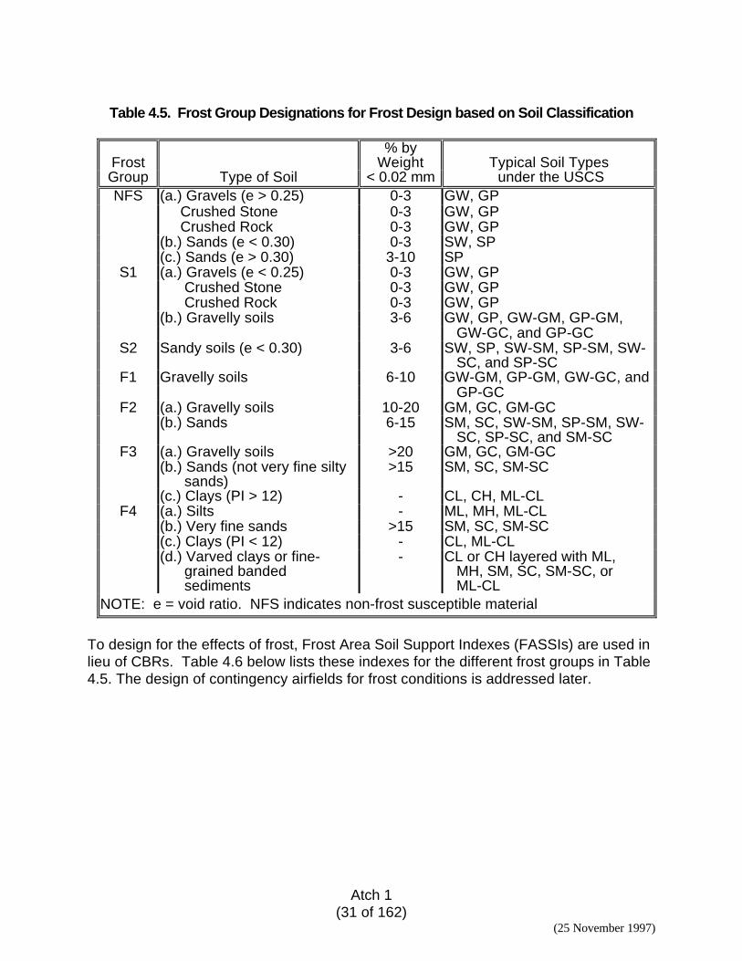
Table 4.5. Frost Group Designations for Frost Design based on Soil Classification
Frost% by
Weight Typical Soil TypesGroup Type of Soil < 0.02 mm under the USCSNFS (a.) Gravels (e > 0.25) 0-3 GW, GP
Crushed Stone 0-3 GW, GP Crushed Rock 0-3 GW, GP(b.) Sands (e < 0.30) 0-3 SW, SP(c.) Sands (e > 0.30) 3-10 SP
S1 (a.) Gravels (e < 0.25) 0-3 GW, GP Crushed Stone 0-3 GW, GP Crushed Rock 0-3 GW, GP(b.) Gravelly soils 3-6 GW, GP, GW-GM, GP-GM,
GW-GC, and GP-GCS2 Sandy soils (e < 0.30) 3-6 SW, SP, SW-SM, SP-SM, SW-
SC, and SP-SCF1 Gravelly soils 6-10 GW-GM, GP-GM, GW-GC, and
GP-GCF2 (a.) Gravelly soils 10-20 GM, GC, GM-GC
(b.) Sands 6-15 SM, SC, SW-SM, SP-SM, SW- SC, SP-SC, and SM-SC
F3 (a.) Gravelly soils >20 GM, GC, GM-GC(b.) Sands (not very fine silty sands)
>15 SM, SC, SM-SC
(c.) Clays (PI > 12) - CL, CH, ML-CLF4 (a.) Silts - ML, MH, ML-CL
(b.) Very fine sands >15 SM, SC, SM-SC(c.) Clays (PI < 12) - CL, ML-CL(d.) Varved clays or fine- grained banded sediments
- CL or CH layered with ML, MH, SM, SC, SM-SC, or ML-CL
NOTE: e = void ratio. NFS indicates non-frost susceptible material
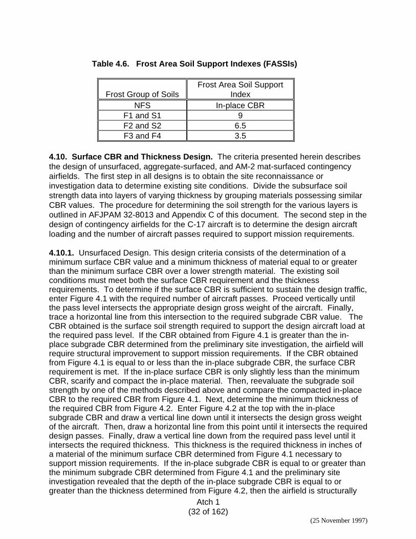
To design for the effects of frost, Frost Area Soil Support Indexes (FASSIs) are used inlieu of CBRs. Table 4.6 below lists these indexes for the different frost groups in Table4.5. The design of contingency airfields for frost conditions is addressed later.
Atch 1(32 of 162)
(25 November 1997)
Table 4.6. Frost Area Soil Support Indexes (FASSIs)
Frost Group of SoilsFrost Area Soil Support
IndexNFS In-place CBR
F1 and S1 9F2 and S2 6.5F3 and F4 3.5
4.10. Surface CBR and Thickness Design. The criteria presented herein describesthe design of unsurfaced, aggregate-surfaced, and AM-2 mat-surfaced contingencyairfields. The first step in all designs is to obtain the site reconnaissance orinvestigation data to determine existing site conditions. Divide the subsurface soilstrength data into layers of varying thickness by grouping materials possessing similarCBR values. The procedure for determining the soil strength for the various layers isoutlined in AFJPAM 32-8013 and Appendix C of this document. The second step in thedesign of contingency airfields for the C-17 aircraft is to determine the design aircraftloading and the number of aircraft passes required to support mission requirements.
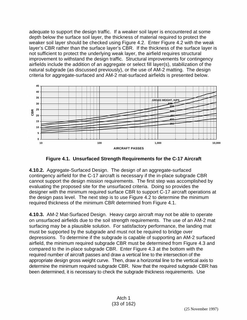
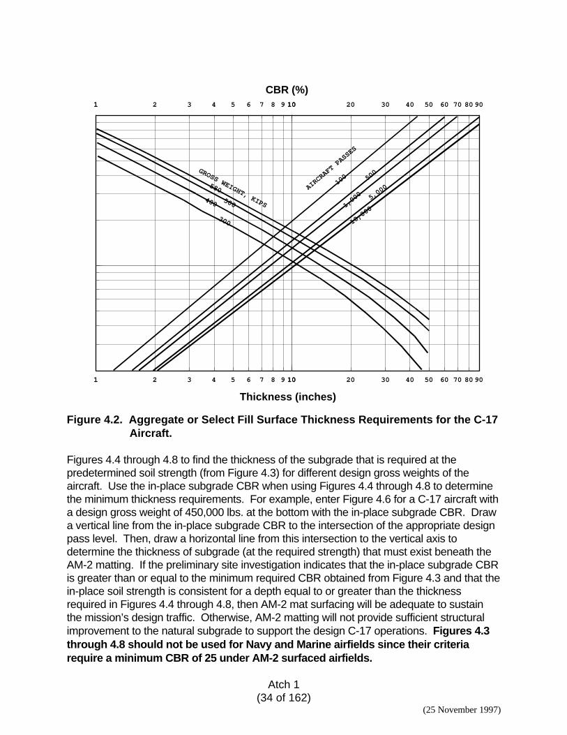
4.10.1. Unsurfaced Design. This design criteria consists of the determination of aminimum surface CBR value and a minimum thickness of material equal to or greaterthan the minimum surface CBR over a lower strength material. The existing soilconditions must meet both the surface CBR requirement and the thicknessrequirements. To determine if the surface CBR is sufficient to sustain the design traffic,enter Figure 4.1 with the required number of aircraft passes. Proceed vertically untilthe pass level intersects the appropriate design gross weight of the aircraft. Finally,trace a horizontal line from this intersection to the required subgrade CBR value. TheCBR obtained is the surface soil strength required to support the design aircraft load atthe required pass level. If the CBR obtained from Figure 4.1 is greater than the in-place subgrade CBR determined from the preliminary site investigation, the airfield willrequire structural improvement to support mission requirements. If the CBR obtainedfrom Figure 4.1 is equal to or less than the in-place subgrade CBR, the surface CBRrequirement is met. If the in-place surface CBR is only slightly less than the minimumCBR, scarify and compact the in-place material. Then, reevaluate the subgrade soilstrength by one of the methods described above and compare the compacted in-placeCBR to the required CBR from Figure 4.1. Next, determine the minimum thickness ofthe required CBR from Figure 4.2. Enter Figure 4.2 at the top with the in-placesubgrade CBR and draw a vertical line down until it intersects the design gross weightof the aircraft. Then, draw a horizontal line from this point until it intersects the requireddesign passes. Finally, draw a vertical line down from the required pass level until itintersects the required thickness. This thickness is the required thickness in inches ofa material of the minimum surface CBR determined from Figure 4.1 necessary tosupport mission requirements. If the in-place subgrade CBR is equal to or greater thanthe minimum subgrade CBR determined from Figure 4.1 and the preliminary siteinvestigation revealed that the depth of the in-place subgrade CBR is equal to orgreater than the thickness determined from Figure 4.2, then the airfield is structurally
Atch 1(33 of 162)
(25 November 1997)
adequate to support the design traffic. If a weaker soil layer is encountered at somedepth below the surface soil layer, the thickness of material required to protect theweaker soil layer should be checked using Figure 4.2. Enter Figure 4.2 with the weaklayer’s CBR rather than the surface layer’s CBR. If the thickness of the surface layer isnot sufficient to protect the underlying weak layer, the airfield requires structuralimprovement to withstand the design traffic. Structural improvements for contingencyairfields include the addition of an aggregate or select fill layer(s), stabilization of thenatural subgrade (as discussed previously), or the use of AM-2 matting. The designcriteria for aggregate-surfaced and AM-2 mat-surfaced airfields is presented below.
0
5
10
15
20
25
30
35
40
45
10 100 1,000 10,000
AIRCRAFT PASSES
CB
R
GROSS WEIGHT, KIPS580
550
500
450400
350
Figure 4.1. Unsurfaced Strength Requirements for the C-17 Aircraft
4.10.2. Aggregate-Surfaced Design. The design of an aggregate-surfacedcontingency airfield for the C-17 aircraft is necessary if the in-place subgrade CBRcannot support the design mission requirements. The first step was accomplished byevaluating the proposed site for the unsurfaced criteria. Doing so provides thedesigner with the minimum required surface CBR to support C-17 aircraft operations atthe design pass level. The next step is to use Figure 4.2 to determine the minimumrequired thickness of the minimum CBR determined from Figure 4.1.
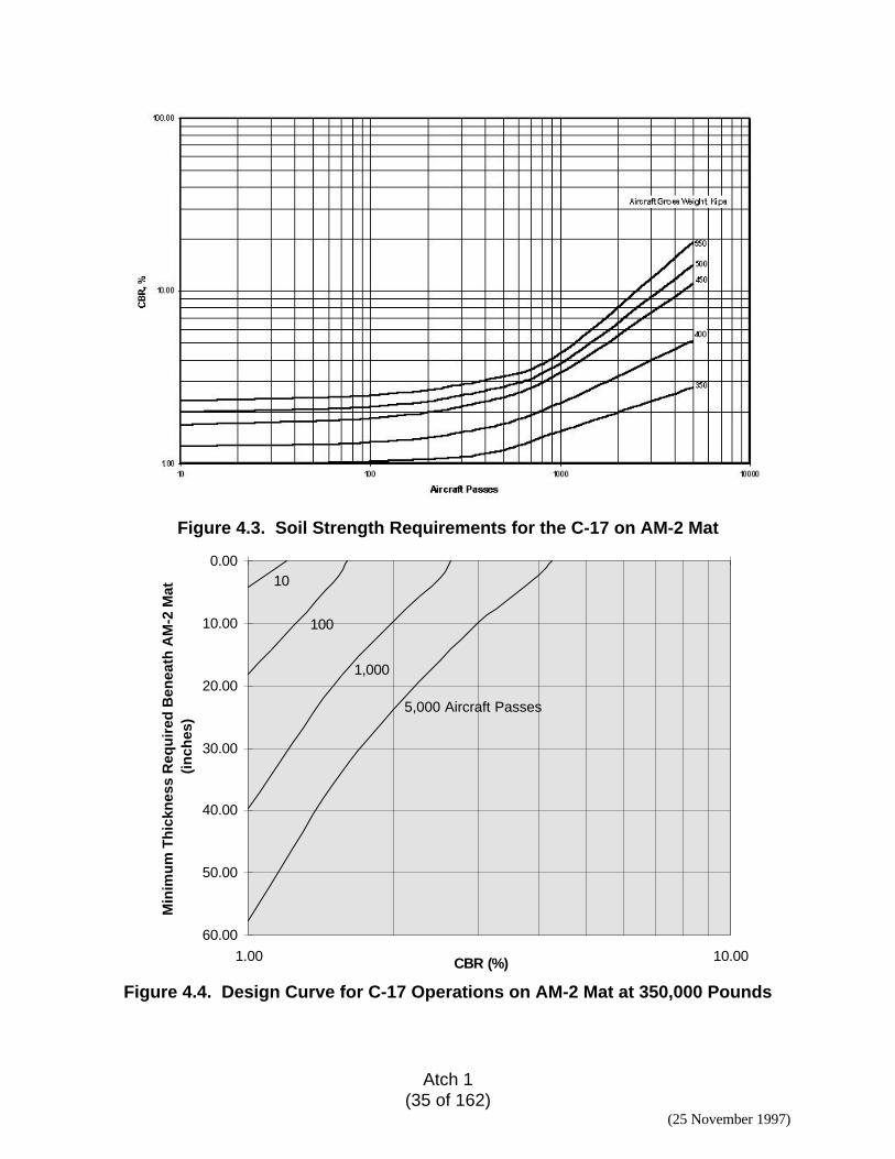
4.10.3. AM-2 Mat-Surfaced Design. Heavy cargo aircraft may not be able to operateon unsurfaced airfields due to the soil strength requirements. The use of an AM-2 matsurfacing may be a plausible solution. For satisfactory performance, the landing matmust be supported by the subgrade and must not be required to bridge overdepressions. To determine if the subgrade is capable of supporting an AM-2 surfacedairfield, the minimum required subgrade CBR must be determined from Figure 4.3 andcompared to the in-place subgrade CBR. Enter Figure 4.3 at the bottom with therequired number of aircraft passes and draw a vertical line to the intersection of theappropriate design gross weight curve. Then, draw a horizontal line to the vertical axis todetermine the minimum required subgrade CBR. Now that the required subgrade CBR hasbeen determined, it is necessary to check the subgrade thickness requirements. Use
Atch 1(34 of 162)
(25 November 1997)
1 2 3 4 5 6 7 8 9 10 20 30 40 50 60 70 80 901 10
Thickness (inches)
1 2 3 4 5 6 7 8 9 10 20 30 40 50 60 70 80 901 10
CBR (%)
580
500400
300
100 50
0
1,000 5,
000
10,000
AIRCRAFT PASSES
GROSS WEIGHT, KIPS
Figure 4.2. Aggregate or Select Fill Surface Thickness Requirements for the C-17Aircraft.
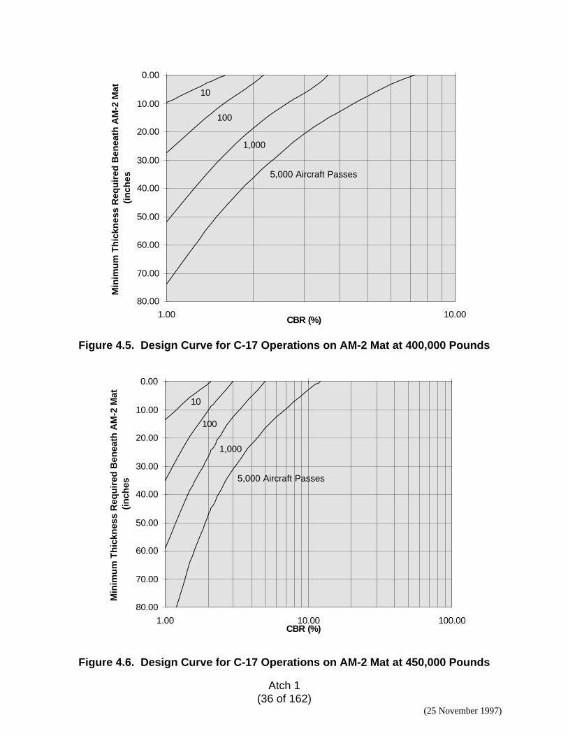
Figures 4.4 through 4.8 to find the thickness of the subgrade that is required at thepredetermined soil strength (from Figure 4.3) for different design gross weights of theaircraft. Use the in-place subgrade CBR when using Figures 4.4 through 4.8 to determinethe minimum thickness requirements. For example, enter Figure 4.6 for a C-17 aircraft witha design gross weight of 450,000 lbs. at the bottom with the in-place subgrade CBR. Drawa vertical line from the in-place subgrade CBR to the intersection of the appropriate designpass level. Then, draw a horizontal line from this intersection to the vertical axis todetermine the thickness of subgrade (at the required strength) that must exist beneath theAM-2 matting. If the preliminary site investigation indicates that the in-place subgrade CBRis greater than or equal to the minimum required CBR obtained from Figure 4.3 and that thein-place soil strength is consistent for a depth equal to or greater than the thicknessrequired in Figures 4.4 through 4.8, then AM-2 mat surfacing will be adequate to sustainthe mission’s design traffic. Otherwise, AM-2 matting will not provide sufficient structuralimprovement to the natural subgrade to support the design C-17 operations. Figures 4.3through 4.8 should not be used for Navy and Marine airfields since their criteriarequire a minimum CBR of 25 under AM-2 surfaced airfields.
Atch 1(35 of 162)
(25 November 1997)
Figure 4.3. Soil Strength Requirements for the C-17 on AM-2 Mat
0.00
10.00
20.00
30.00
40.00
50.00
60.00
1.00 10.00CBR (%)
Min
imu
m T
hic
knes
s R
equ
ired
Ben
eath
AM
-2 M
at
(in
ches
)
10
100
1,000
5,000 Aircraft Passes
Figure 4.4. Design Curve for C-17 Operations on AM-2 Mat at 350,000 Pounds
Atch 1(36 of 162)
(25 November 1997)
0.00
10.00
20.00
30.00
40.00
50.00
60.00
70.00
80.001.00 10.00
CBR (%)
Min
imu
m T
hic
knes
s R
equ
ired
Ben
eath
AM
-2 M
at
(in
ches
10
100
1,000
5,000 Aircraft Passes
Figure 4.5. Design Curve for C-17 Operations on AM-2 Mat at 400,000 Pounds
0.00
10.00
20.00
30.00
40.00
50.00
60.00
70.00
80.00
1.00 10.00 100.00CBR (%)
Min
imu
m T
hic
knes
s R
equ
ired
Ben
eath
AM
-2 M
at
(in
ches
10
100
1,000
5,000 Aircraft Passes
Figure 4.6. Design Curve for C-17 Operations on AM-2 Mat at 450,000 Pounds
Atch 1(37 of 162)
(25 November 1997)
0.00
10.00
20.00
30.00
40.00
50.00
60.00
70.00
80.001.00 10.00 100.00
CBR (%)
Min
imu
m T
hic
knes
s R
equ
ired
Ben
eath
AM
-2 M
at
(in
ches
10
100
1,000
5,000 Aircraft Passes
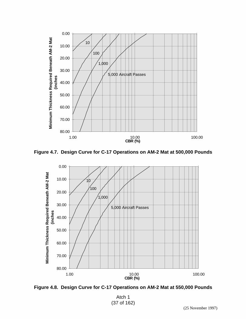
Figure 4.7. Design Curve for C-17 Operations on AM-2 Mat at 500,000 Pounds
0.00
10.00
20.00
30.00
40.00
50.00
60.00
70.00
80.00
1.00 10.00 100.00CBR (%)
Min
imu
m T
hic
knes
s R
equ
ired
Ben
eath
AM
-2 M
at
(in
ches
10
100
1,000
5,000 Aircraft Passes
Figure 4.8. Design Curve for C-17 Operations on AM-2 Mat at 550,000 Pounds
Atch 1(38 of 162)
(25 November 1997)
4.10.4. Design for Frost Conditions. Typically, contingency airfields are not designedfor protection against frost action due to their short design life. However, in somecontingency situations, designing for frost conditions may be warranted. The design forfrost conditions utilizes the reduced subgrade strength criteria which assigns a materialto a frost group based upon the material’s properties. Table 4.5 shows the frost groupdesignations for various material types. Each material is then assigned a Frost AreaSoil Support Index (FASSI) number based upon its frost group designation. The FASSInumbers for each frost group are illustrated in Table 4.6. The material’s FASSI numberis then used in lieu of the in-place subgrade CBR to enter the design curves.Therefore, to design for frost conditions determine the material’s FASSI number, thenperform a typical contingency design utilizing the FASSI number instead of the in-placesubgrade CBR. However, if the FASSI designation is greater than the in-place soil’sCBR, the in-place soil’s CBR should be used for the final design. For a more detailedfrost design refer to AFM 88-6, Chapter 4.
4.11. Design Examples. To illustrate usage of the design criteria outlined above,several examples are provided below for designing contingency airfields for various C-17 aircraft missions.
4.11.1. Example 1. Design an airfield in the theater of operations for 200 operations ofa C-17. A special tactics team determined that the soil’s in-place CBR was 16 for adepth of approximately 24 inches beyond which there is a 12-inch layer of 10 CBRmaterial. The airfield’s geometric design does not include a parallel taxiway.
Note: The number of required passes should be multiplied by two to accountfor the aircraft taxiing down the runway to takeoff or unload cargo.
Step 1. The design aircraft has been designated as the C-17. The design grossweight of the C-17 is 447 kips which seems reasonable in regard to missionrequirements.
Step 2. The design aircraft passes stated were 200, however, for designpurposes (as noted above) 400 passes will be used to account for taximovements.
Step 3. Using Figure 4.1, determine the minimum required subgrade strength tosupport 400 passes of a 447 kip C-17 aircraft. Enter Figure 4.1 with 400 passesand draw a vertical line to just below the 450 kip gross weight curve. From thispoint, draw a horizontal line to the vertical axis to determine the required CBR.The required subgrade CBR for 400 passes of a 447 kip C-17 is approximately15 CBR.
Step 4. Since the minimum required CBR is less than the in-place CBR (15 <16), then the in-place subgrade surface strength is sufficient to support mission
Atch 1(39 of 162)
(25 November 1997)
requirements. It must also be determined if adequate thickness of the 16 CBRmaterial is available. Enter Figure 4.2 at the top with the in-place subgrade CBR(16) and draw a vertical line down until it intersects the design gross weight ofthe C-17 or 447 kips. Next, draw a horizontal line from this intersection until itintersects the design pass level of 400 passes. Finally, draw a vertical line fromthis intersection downward until you intercept the required thickness. Seveninches of 16 CBR material is required to support 400 passes of a 447 kip C-17aircraft. Since the in-place soil has 24 inches of 16 CBR material, theunsurfaced airfield can support the design aircraft for the design passes withoutstructural improvement.
Step 5. Since there is a 12-inch layer of weaker material underlying the surfacelayer, it must be determined if the surface soil layer has adequate thickness toprotect the underlying weaker layer. Enter Figure 4.2 with the weak layer’s CBR(10) and draw a vertical line down until it intersects the design gross weight ofthe aircraft or 447 kips. Next, draw a horizontal line from this intersection until itintersects the design pass level of 400 passes. Finally, draw a vertical line fromthis intersection downward until you intercept the required material thickness.Nine inches of a 15 CBR material is required to protect the weak subsurface soillayer. Since the in-place soil has 24 inches of a 16 CBR material, the weaklayer is adequately protected and the design is valid.
4.11.2. Example 2. Developments in the theater of operations require the design of asecond contingency airfield to support 200 passes of a C-17. The special tactics teamdetermined that the soil’s in-place CBR at the second site is 12 for a depth ofapproximately 20 inches beyond which the CBR of the material increased. This airfieldwill not possess a parallel taxiway.
Step 1. The design aircraft has been designated as the C-17. The design grossweight of the C-17 is 447 kips which seems reasonable in regard to missionrequirements.
Step 2. The design aircraft passes stated were 200, however, for designpurposes (as noted in Example 1) 400 passes will be used to account for taximovements.
Step 3. Using Figure 4.1, determine the minimum required subgrade strength tosupport 400 passes of a 447 kip C-17 aircraft. Enter Figure 4.1 with 400 passesand draw a vertical line to just below the 450 kip gross weight curve. From thispoint, draw a horizontal line to the vertical axis to determine the required CBR.The required subgrade CBR for 400 passes of a 447 kip C-17 is approximately15 CBR.
Step 4. Since the required CBR is greater than the in-place CBR (15 > 12), thenthe subgrade must be improved structurally to support mission requirements.First, determine the thickness of 15 CBR material required above the subgrade
Atch 1(40 of 162)
(25 November 1997)
to support mission requirements. Enter Figure 4.2 at the top with the in-placesubgrade CBR (12) and draw a vertical line down until it intersects the designgross weight of the C-17 or 447 kips. Next, draw a horizontal line from thisintersection until it intersects the design pass level of 400 passes. Finally, drawa vertical line from this intersection downward until you intercept the requiredthickness. The design requires 8 inches of 15 CBR material be placed over thein-place subgrade in order to support 400 passes of a 447 kip C-17 aircraft.
4.11.3. Example 3. Developments have led to the need for a contingency airfield.Estimation of the mission suggests that the design pass level should be 1,000 passesof a 447 kip C-17. The only available site has a CBR of 4 for a depth of 12 incheswhere it increases to an 8 CBR for an additional 24 inches.
Note: The mission requirements include plans for a parallel taxiway and asmall apron. Thus, the number of required passes should remain at1,000 due to the probability that the aircraft will use the taxiway andapron for all movements other than takeoffs or landings.
Step 1. The design aircraft has been designated as the C-17. The design grossweight of the C-17 is 447 kips which seems reasonable in regard to missionrequirements.
Step 2. The design aircraft passes stated were 1,000. All pavements are A typetraffic areas and will use the same design.
Step 3. Using Figure 4.1, determine the minimum required subgrade strength tosupport 1,000 passes of a 447 kip C-17 aircraft. Enter Figure 4.1 with 1,000passes and draw a vertical line to just below the 450 kip gross weight curve.From this point, draw a horizontal line to the vertical axis to determine theminimum required CBR. The required subgrade CBR for 1,000 passes of a 447kip C-17 is approximately 18 CBR.
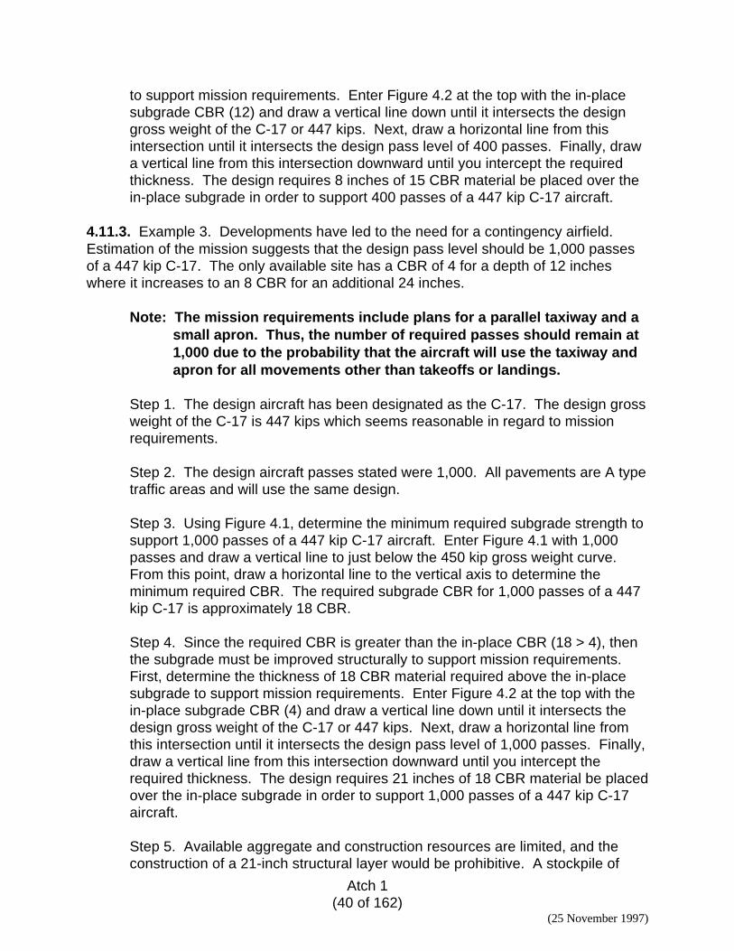
Step 4. Since the required CBR is greater than the in-place CBR (18 > 4), thenthe subgrade must be improved structurally to support mission requirements.First, determine the thickness of 18 CBR material required above the in-placesubgrade to support mission requirements. Enter Figure 4.2 at the top with thein-place subgrade CBR (4) and draw a vertical line down until it intersects thedesign gross weight of the C-17 or 447 kips. Next, draw a horizontal line fromthis intersection until it intersects the design pass level of 1,000 passes. Finally,draw a vertical line from this intersection downward until you intercept therequired thickness. The design requires 21 inches of 18 CBR material be placedover the in-place subgrade in order to support 1,000 passes of a 447 kip C-17aircraft.
Step 5. Available aggregate and construction resources are limited, and theconstruction of a 21-inch structural layer would be prohibitive. A stockpile of
Atch 1(41 of 162)
(25 November 1997)
AM-2 landing mat is available, and a decision is made to determine theplausibility of an AM-2 mat-surfaced airfield. First, determine the minimumsubgrade surface CBR requirements beneath the landing mat from Figure 4.3.Enter the chart at the bottom with the design aircraft passes (1,000) and draw avertical line until it intersects the design gross weight of the aircraft. From thisintersection, draw a horizontal line across to the vertical axis to determine theminimum subgrade CBR that is required beneath the AM-2 mat. The requiredsubgrade CBR for 1,000 passes of a 447 kip C-17 on AM-2 landing mat is 3.2CBR or ~ 3.5 CBR.
Step 6. Since the required subgrade CBR beneath the AM-2 matting is less thanthe existing in-place subgrade CBR (3.5 < 4), the surface CBR requirements aremet. Next, determine the minimum thickness of the subgrade required tosupport the mission’s design traffic. Enter Figure 4.6 for a 450 kip C-17 with thein-place CBR of 4 and draw a vertical line until it intersects the design pass levelof 1,000. Then, draw a horizontal line until it intersects the vertical axis todetermine the minimum thickness of 4 CBR material required beneath the AM-2matting. A thickness of 5 inches of 4 CBR material is required beneath the AM-2mat to support 1,000 passes of a 447 kip C-17. Since the in-place CBR of 4exists for a depth of 12 inches, the thickness requirements beneath AM-2 matare met and AM-2 mat-surfacing is sufficient to support the design missiontraffic.
4.11.4. Example 4. Information provided by headquarters indicates that the airfield inExample 3 will be required to support 5,000 passes of a C-17 rather than the original1,000 passes. Redesign the airfield accordingly.
Step 1. The design aircraft and its design gross weight are denoted above as a447 kip C-17.
Step 2. Due to changes in mission requirements, the design pass level wasincreased from 1,000 passes to 5,000 passes.
Step 3. Following the guidance in Step 3 of the example above, the unsurfacedcriteria minimum surface CBR requirement is determined to be a 23 CBR. Sincethe in-place subgrade CBR is much less than the required subgrade CBR (4 <23), the in-place subgrade must be improved structurally to support the mission’sdesign traffic.
Step 4. Use the guidance in step 4 of the above example to determine theminimum required thickness of an aggregate or select fill layer of at least a 23CBR to be placed above the in-place subgrade material. The criteria in Figure4.2 indicate that approximately 25 inches of a 23 CBR material is required tosupport 5,000 passes of a 447 kip C-17.
Atch 1(42 of 162)
(25 November 1997)
Step 5. Since logistics prohibits the use of a large amount of fill, AM-2 mat-surfacing should be considered. As shown in step 5 above, determine theminimum surface subgrade CBR required to support AM-2 matting for the designmission traffic. From Figure 4.3, it is determined that a 10 CBR material isrequired to support mission requirements. Since the in-place subgrade CBR isless than the required CBR (4 < 10), the in-place subgrade must be structurallyimproved.
Step 6. To determine the thickness required of the 10 CBR material, use theguidance in step 6 above and Figure 4.6. Entering the figure with the in-placesubgrade CBR (4) indicates that 22 inches of a 10 CBR is required beneath theAM-2 mat to support design traffic requirements.
Thus, the design of the airfield includes the construction of a 22-inch select fill oraggregate layer of at least a 10 CBR to be placed on top of the 4 CBR in-placesubgrade. The surfacing will consist of the use of AM-2 matting for all traffic areas.Alternate designs incorporating various layers of differing soil strengths may beconsidered provided that they meet the criteria presented herein.
4.11.5. Example 5. Design an airfield for contingency operations of a C-17 in an areasusceptible to frost action. 50 passes are expected during the spring thaw period.Preliminary site investigations identified that the subgrade was classified as a low-plasticity clay (CL) with a Plasticity Index (PI) of 15 and an in-place subgrade CBR of10 for 36 inches. No taxiways will be constructed.
Step 1. The design aircraft is a 447 kip C-17.
Step 2. The expected number of aircraft passes is 50, but the airfield will nothave any taxiways so the design pass level is adjusted to 100 (see Note inExample 1).
Step 3. The first step in designing for frost is to determine the Frost Group towhich the subgrade belongs. Using the site investigation data and Table 4.1, itis determined that the subgrade is in the F3 Frost Group. The next step is todetermine the Frost Area Soil Support Index (FASSI) for the subgrade. UsingTable 4.2, the FASSI for an F3 material is 3.5.
Step 4. Since the FASSI is less than the in-place subgrade CBR (3.5 < 10), thenthe FASSI must be used in lieu of the in-place CBR for determining soil strengthand thickness requirements. Enter Figure 4.1 with the design passes (100) andthe gross aircraft weight (447 kips) to determine the subgrade surface CBRrequired to support the design mission traffic. Following the steps in Example 1,Step 3, it is determined that a minimum surface CBR of 12 is required to support100 passes of a 447 kip C-17.
Atch 1(43 of 162)
(25 November 1997)
Step 5. Since the minimum required surface CBR is greater than the in-placesubgrade CBR for frost design (12 > 3.5), the subgrade requires structuralimprovement to withstand the design traffic. Using Figure 4.2, enter the chartwith an in-place subgrade CBR of 3.5 to determine the thickness of 12 CBRmaterial required above the subgrade to support the design traffic. Followingthe guidance in Example 1, Step 4, it is determined that 15 inches of 12 CBRmaterial is required above the 3.5 CBR (frost) subgrade.
At this point, an analysis of available construction materials would determine whether15 inches of an 12 CBR non frost-susceptible material would be plausible. If not, thedesign procedure for the use of AM-2 matting should proceed if sufficient mat isavailable. Otherwise, alternate means of strengthening the in-place subgrade shouldbe explored as discussed earlier.
4.12. Drainage Design. Adequate surface drainage should be provided in order tominimize moisture damage to the airfield. The rapid removal of surface water reducesthe potential for absorption and helps to ensure more consistent soil strength. Thesurface geometry of the airfield should be designed so that drainage is provided at allpoints. Depending upon the surrounding terrain, surface drainage may be achieved bya continual cross slope or by an interconnected series of cross slopes. Except inspecial circumstances the two year storm frequency is considered a satisfactory designfrequency for contingency airfields. Design of surface drainage should be inaccordance with TM 5-820-3/AFM 88-5, Chapter 3. Requirements for subsurfacedrainage are outlined in TM 5-820-2/AFM 88-5, Chapter 2.
4.13. Dust Control. The primary objective of a dust palliative is to prevent soilparticles from becoming airborne as a result of wind or traffic. Dust palliatives must beable to withstand the abrasion of wheels and tracks. The abrasive action of aircraftlanding gear may be too serious for the use of some dust palliatives. However, the useof dust palliatives in non-braking areas should be considered especially in arid andsemi-arid climates. No one product has been identified as universally acceptable for allproblem situations that may be encountered. Several materials have beenrecommended for use and are discussed in TM 5-830-3/AFM 88-17, Chapter 3.
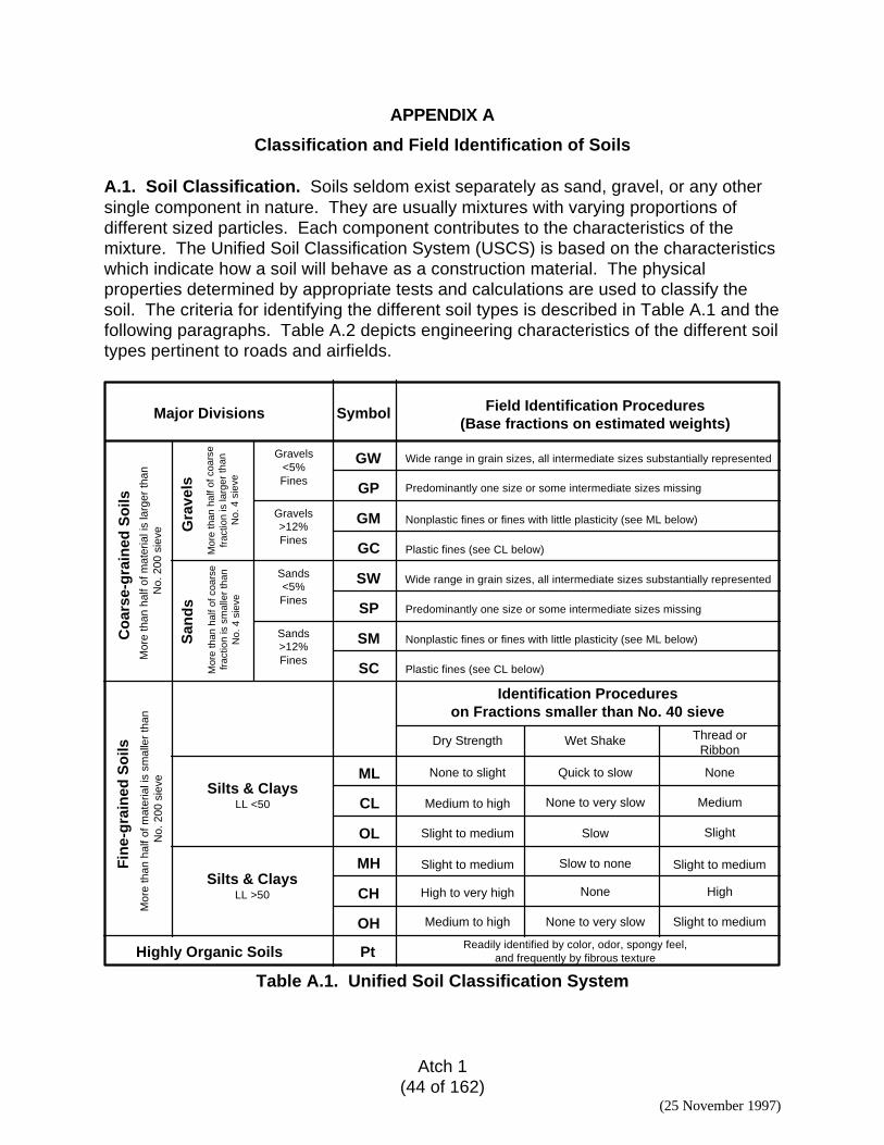
Atch 1(44 of 162)
(25 November 1997)
APPENDIX A
Classification and Field Identification of Soils
A.1. Soil Classification. Soils seldom exist separately as sand, gravel, or any othersingle component in nature. They are usually mixtures with varying proportions ofdifferent sized particles. Each component contributes to the characteristics of themixture. The Unified Soil Classification System (USCS) is based on the characteristicswhich indicate how a soil will behave as a construction material. The physicalproperties determined by appropriate tests and calculations are used to classify thesoil. The criteria for identifying the different soil types is described in Table A.1 and thefollowing paragraphs. Table A.2 depicts engineering characteristics of the different soiltypes pertinent to roads and airfields.
Major Divisions Symbol Field Identification Procedures(Base fractions on estimated weights)
GW
GP
GM
GC
SW
SP
SM
SC
ML
CL
OL
MH
CH
OH
Pt
Gravels<5%Fines
Sands<5%Fines
Sands>12%Fines
Gravels>12%Fines
Silts & ClaysLL <50
Silts & ClaysLL >50
Highly Organic Soils
Fin
e-g
rain
ed S
oils
Co
arse
-gra
ined
So
ils
Gra
vels
San
ds
Mor
e th
an h
alf o
f coa
rse
frac
tion
is la
rger
than
No.
4 s
ieve
Mor
e th
an h
alf o
f coa
rse
frac
tion
is s
mal
ler
than
No.
4 s
ieve
Mor
e th
an h
alf o
f mat
eria
l is
larg
er th
an
No.
200
sie
veM
ore
than
hal
f of m
ater
ial i
s sm
alle
r th
an
No.
200
sie
ve
Readily identified by color, odor, spongy feel,and frequently by fibrous texture
Wide range in grain sizes, all intermediate sizes substantially represented
Nonplastic fines or fines with little plasticity (see ML below)
Plastic fines (see CL below)
Wide range in grain sizes, all intermediate sizes substantially represented
Predominantly one size or some intermediate sizes missing
Nonplastic fines or fines with little plasticity (see ML below)
Plastic fines (see CL below)
Identification Procedureson Fractions smaller than No. 40 sieve
Predominantly one size or some intermediate sizes missing
Dry Strength Wet Shake Thread orRibbon
None to slight
Medium to high
Slight to medium
Slight to medium
High to very high
Medium to high
Quick to slow
None to very slow
Slow
Slow to none
None
None to very slow
None
Medium
Slight
Slight to medium
High
Slight to medium
Table A.1. Unified Soil Classification System
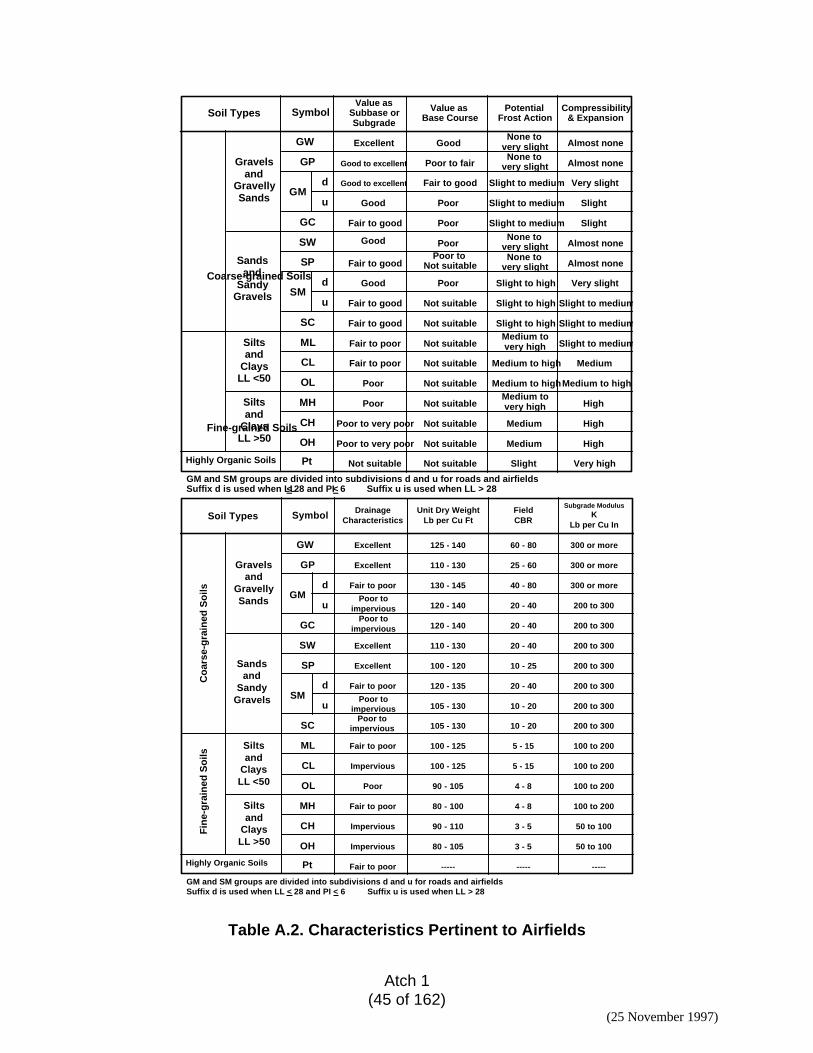
Atch 1(45 of 162)
(25 November 1997)
Soil Types Symbol
GW
GP
GM
GC
SW
SP
SM
SC
ML
CL
OL
MH
CH
OH
Pt
Siltsand
ClaysLL <50
Siltsand
ClaysLL >50
Highly Organic Soils
Fine-grained Soils
Coarse-grained Soils
Gravelsand
GravellySands
Sandsand
SandyGravels
d
u
d
u
GM and SM groups are divided into subdivisions d and u for roads and airfieldsSuffix d is used when LL< 28 and PI< 6 Suffix u is used when LL > 28
Value asSubbase orSubgrade
Value asBase Course
PotentialFrost Action
Compressibility& Expansion
Excellent
Good to excellent
Good to excellent
Good
Good
Good
Good
Fair to good
Fair to good
Fair to good
Fair to good
Fair to good
Fair to poor
Fair to poor
Poor
Poor
Poor
Poor
Poor
Poor
Poor to fair
Poor toNot suitable
Not suitable
Not suitable
Not suitable
Not suitable Not suitable
Not suitable
Not suitable
Not suitable
Not suitable
Not suitable
Poor to very poor
Poor to very poor
None tovery slightNone to
very slight
None tovery slightNone to
very slight
Slight to medium
Slight to medium
Slight to medium
Slight to medium
Slight to medium
Slight to medium
Slight to high
Slight to high
Slight to highMedium tovery high
Medium tovery high
Medium to high
Medium to highMedium to high
Medium
Medium
Medium
Slight
Slight
Slight
Almost none
Almost none
Almost none
Almost none
Very slight
Very slight
High
High
High
Very high
Soil Types Symbol
GW
GP
GM
GC
SW
SP
SM
SC
ML
CL
OL
MH
CH
OH
Pt
Siltsand
ClaysLL <50
Siltsand
ClaysLL >50
Highly Organic Soils
Fin
e-g
rain
ed S
oils
Co
arse
-gra
ined
So
ils
Gravelsand
GravellySands
Sandsand
SandyGravels
d
u
d
u
GM and SM groups are divided into subdivisions d and u for roads and airfieldsSuffix d is used when LL < 28 and PI < 6 Suffix u is used when LL > 28
DrainageCharacteristics
Unit Dry WeightLb per Cu Ft
FieldCBR
Subgrade ModulusK
Lb per Cu In
Excellent
Excellent
Excellent
Excellent
Fair to poor
Fair to poor
Fair to poor
Fair to poor
Fair to poor ----- ----- -----
Impervious
Impervious
Impervious
Poor
Poor toimpervious
Poor toimpervious
Poor toimpervious
Poor toimpervious
125 - 140
110 - 130
130 - 145
120 - 140
120 - 140
110 - 130
100 - 120
120 - 135
105 - 130
105 - 130
60 - 80
25 - 60
40 - 80
20 - 40
20 - 40
20 - 40
10 - 25
20 - 40
10 - 20
10 - 20
300 or more
300 or more
300 or more
200 to 300
200 to 300
200 to 300
200 to 300
200 to 300
200 to 300
200 to 300
100 to 200
100 to 200
100 to 200
100 to 200
50 to 100
50 to 100
100 - 125
100 - 125
90 - 105
90 - 110
80 - 105
80 - 100
5 - 15
5 - 15
4 - 8
4 - 8
3 - 5
3 - 5
Table A.2. Characteristics Pertinent to Airfields
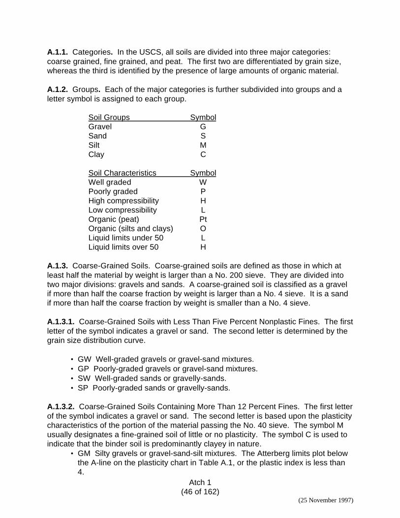
Atch 1(46 of 162)
(25 November 1997)
A.1.1. Categories. In the USCS, all soils are divided into three major categories:coarse grained, fine grained, and peat. The first two are differentiated by grain size,whereas the third is identified by the presence of large amounts of organic material.
A.1.2. Groups. Each of the major categories is further subdivided into groups and aletter symbol is assigned to each group.
Soil Groups SymbolGravel GSand SSilt MClay C
Soil Characteristics SymbolWell graded WPoorly graded PHigh compressibility HLow compressibility LOrganic (peat) PtOrganic (silts and clays) OLiquid limits under 50 LLiquid limits over 50 H
A.1.3. Coarse-Grained Soils. Coarse-grained soils are defined as those in which atleast half the material by weight is larger than a No. 200 sieve. They are divided intotwo major divisions: gravels and sands. A coarse-grained soil is classified as a gravelif more than half the coarse fraction by weight is larger than a No. 4 sieve. It is a sandif more than half the coarse fraction by weight is smaller than a No. 4 sieve.
A.1.3.1. Coarse-Grained Soils with Less Than Five Percent Nonplastic Fines. The firstletter of the symbol indicates a gravel or sand. The second letter is determined by thegrain size distribution curve.
• GW Well-graded gravels or gravel-sand mixtures.• GP Poorly-graded gravels or gravel-sand mixtures.• SW Well-graded sands or gravelly-sands.• SP Poorly-graded sands or gravelly-sands.
A.1.3.2. Coarse-Grained Soils Containing More Than 12 Percent Fines. The first letter
of the symbol indicates a gravel or sand. The second letter is based upon the plasticitycharacteristics of the portion of the material passing the No. 40 sieve. The symbol Musually designates a fine-grained soil of little or no plasticity. The symbol C is used toindicate that the binder soil is predominantly clayey in nature.
• GM Silty gravels or gravel-sand-silt mixtures. The Atterberg limits plot belowthe A-line on the plasticity chart in Table A.1, or the plastic index is less than4.
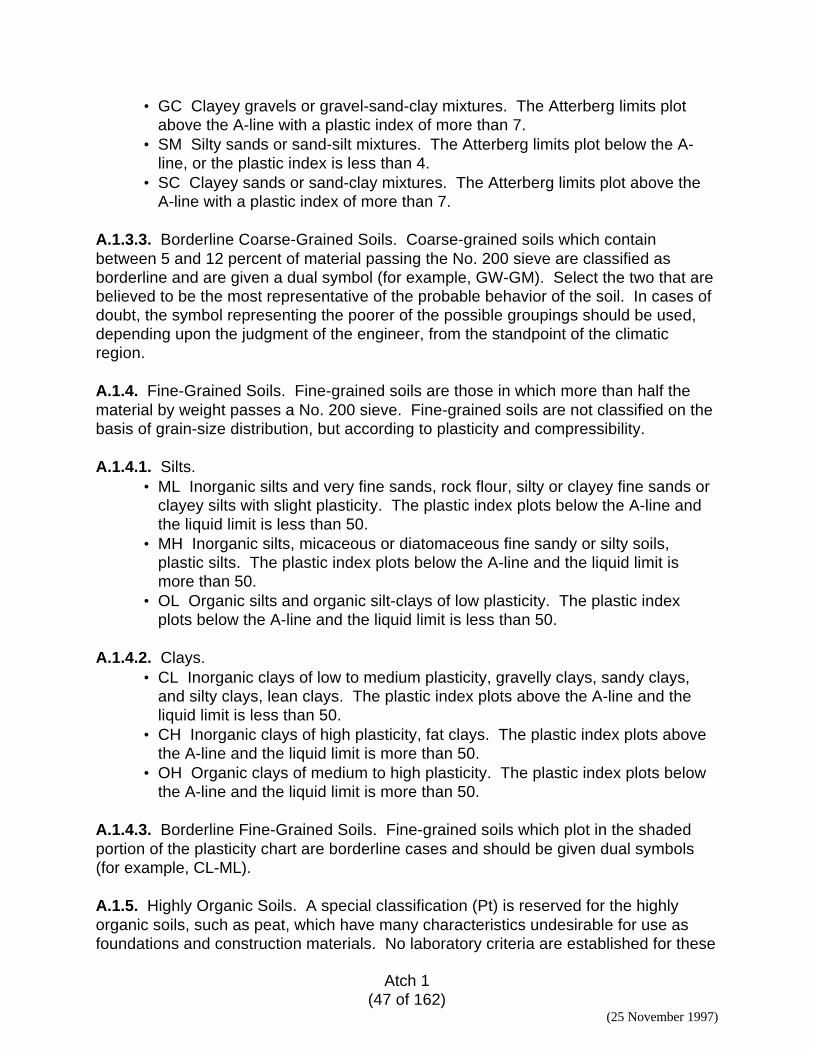
Atch 1(47 of 162)
(25 November 1997)
• GC Clayey gravels or gravel-sand-clay mixtures. The Atterberg limits plotabove the A-line with a plastic index of more than 7.
• SM Silty sands or sand-silt mixtures. The Atterberg limits plot below the A-line, or the plastic index is less than 4.
• SC Clayey sands or sand-clay mixtures. The Atterberg limits plot above theA-line with a plastic index of more than 7.
A.1.3.3. Borderline Coarse-Grained Soils. Coarse-grained soils which containbetween 5 and 12 percent of material passing the No. 200 sieve are classified asborderline and are given a dual symbol (for example, GW-GM). Select the two that arebelieved to be the most representative of the probable behavior of the soil. In cases ofdoubt, the symbol representing the poorer of the possible groupings should be used,depending upon the judgment of the engineer, from the standpoint of the climaticregion.
A.1.4. Fine-Grained Soils. Fine-grained soils are those in which more than half thematerial by weight passes a No. 200 sieve. Fine-grained soils are not classified on thebasis of grain-size distribution, but according to plasticity and compressibility.
A.1.4.1. Silts.• ML Inorganic silts and very fine sands, rock flour, silty or clayey fine sands or
clayey silts with slight plasticity. The plastic index plots below the A-line andthe liquid limit is less than 50.
• MH Inorganic silts, micaceous or diatomaceous fine sandy or silty soils,plastic silts. The plastic index plots below the A-line and the liquid limit ismore than 50.
• OL Organic silts and organic silt-clays of low plasticity. The plastic indexplots below the A-line and the liquid limit is less than 50.
A.1.4.2. Clays.• CL Inorganic clays of low to medium plasticity, gravelly clays, sandy clays,
and silty clays, lean clays. The plastic index plots above the A-line and theliquid limit is less than 50.
• CH Inorganic clays of high plasticity, fat clays. The plastic index plots abovethe A-line and the liquid limit is more than 50.
• OH Organic clays of medium to high plasticity. The plastic index plots belowthe A-line and the liquid limit is more than 50.
A.1.4.3. Borderline Fine-Grained Soils. Fine-grained soils which plot in the shadedportion of the plasticity chart are borderline cases and should be given dual symbols(for example, CL-ML).
A.1.5. Highly Organic Soils. A special classification (Pt) is reserved for the highlyorganic soils, such as peat, which have many characteristics undesirable for use asfoundations and construction materials. No laboratory criteria are established for these
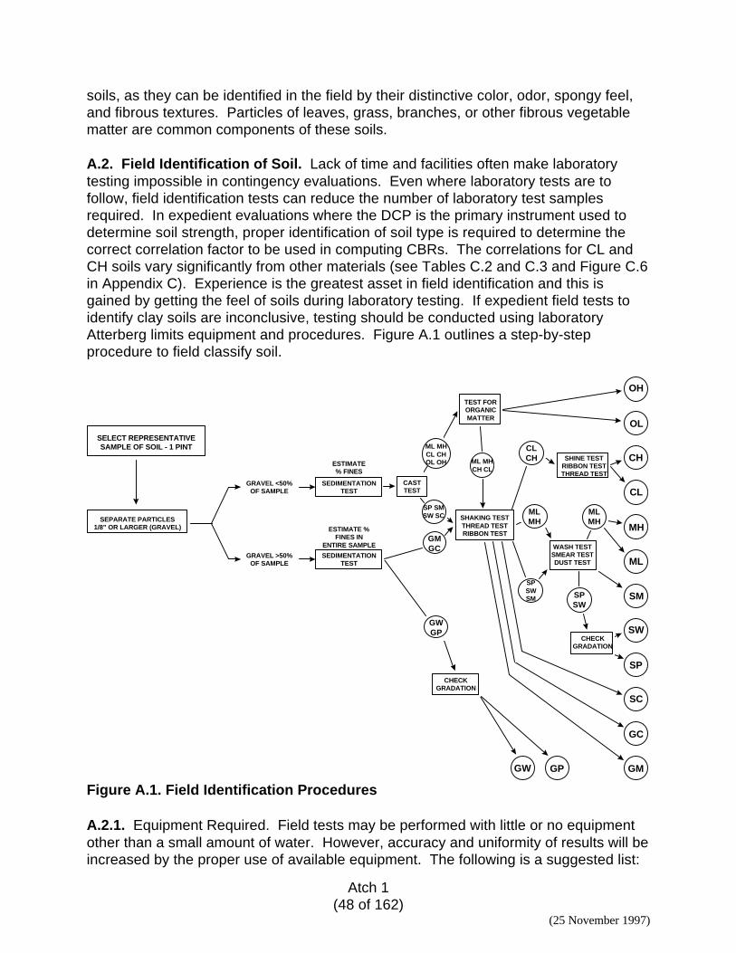
Atch 1(48 of 162)
(25 November 1997)
soils, as they can be identified in the field by their distinctive color, odor, spongy feel,and fibrous textures. Particles of leaves, grass, branches, or other fibrous vegetablematter are common components of these soils.
A.2. Field Identification of Soil. Lack of time and facilities often make laboratorytesting impossible in contingency evaluations. Even where laboratory tests are tofollow, field identification tests can reduce the number of laboratory test samplesrequired. In expedient evaluations where the DCP is the primary instrument used todetermine soil strength, proper identification of soil type is required to determine thecorrect correlation factor to be used in computing CBRs. The correlations for CL andCH soils vary significantly from other materials (see Tables C.2 and C.3 and Figure C.6in Appendix C). Experience is the greatest asset in field identification and this isgained by getting the feel of soils during laboratory testing. If expedient field tests toidentify clay soils are inconclusive, testing should be conducted using laboratoryAtterberg limits equipment and procedures. Figure A.1 outlines a step-by-stepprocedure to field classify soil.
SELECT REPRESENTATIVESAMPLE OF SOIL - 1 PINT
SEPARATE PARTICLES1/8” OR LARGER (GRAVEL)
GRAVEL <50%OF SAMPLE
GRAVEL >50%OF SAMPLE
SEDIMENTATIONTEST
SEDIMENTATIONTEST
ESTIMATE% FINES
ESTIMATE %FINES IN
ENTIRE SAMPLE
CASTTEST
SHAKING TESTTHREAD TESTRIBBON TEST
TEST FORORGANICMATTER
WASH TESTSMEAR TESTDUST TEST
SHINE TESTRIBBON TESTTHREAD TEST
CHECKGRADATION
CHECKGRADATION
OH
OL
CH
CL
MH
ML
SM
SW
SP
SC
GC
GMGPGW
SPSW
MLMH
MLMH
CLCH
GWGP
GMGC
SP SMSW SC
SPSWSM
ML MHCH CL
ML MHCL CHOL OH
Figure A.1. Field Identification Procedures
A.2.1. Equipment Required. Field tests may be performed with little or no equipmentother than a small amount of water. However, accuracy and uniformity of results will beincreased by the proper use of available equipment. The following is a suggested list:
Atch 1(49 of 162)
(25 November 1997)
• Sieves:− No. 40. All tests used to identify the fine-grained portions of any soil are
performed on the portion of the material which passes the No. 40 sieve. Ifthis sieve is not available, a rough separation may be made by spreadingthe material on a flat surface and removing the gravel and larger sandparticles.
− No. 4. This sieve defines the limit between gravels and sands.− No. 200. This sieve defines the limit between sands and fines. The
sedimentation test may also be used to separate the sands and fines. Thistest requires a transparent cup or jar.
• Pan and oven or other heating device.• Mixing bowl and pestle.• Scales or balances.• Knife or small spatula.
A.2.2. Tests for Field Identification. The USCS considers three soil properties: thepercentage of gravel, sand, or fines; the shape of the grain-size distribution curve; andthe plasticity. The purpose of field tests is to get the best possible identification andclassification in the field. Tests appropriate to a given soil sample should be made.When a simple visual examination will define the soil type, only the tests needed toverify this are necessary. When results from a test are inconclusive, some of thesimilar tests should be tried to establish the best identification.
A.2.2.1. Visual Examination. This test should establish the color, grain sizes, grainshapes of the coarse-grained portion, approximate gradation, and some properties ofthe undisturbed soil.
A.2.2.1.1. Color. Color helps in distinguishing between soil types and aids inidentifying soil types. It may also indicate the presence of certain chemicals, minerals,or impurities. Color often varies with moisture content. Thus the moisture content atthe time of identification should be included. Colors generally become darker as themoisture content increases and lighter as the soil dries. Some fine-grained soil (OH,OL) with dark, drab shades of brown or gray, including almost black, contain organicmaterial. In contrast, clean, bright shades of gray, olive green, brown, red, yellow, andwhite are associated with inorganic soils. Gray-blue or gray-and-yellow mottled colorsfrequently result from poor drainage. Red, yellow, and yellowish-brown result from thepresence of iron oxides. White to pink may indicate considerable silica, calciumcarbonate, or aluminum compounds.
A.2.2.1.2. Grain Size. The maximum particle size of each sample should beestablished. This determines the upper limit of the gradation curve. Gravels rangedown to the size of peas. Sands start just below this size and decrease until theindividual grains are just distinguishable by the naked eye. Silt and clay particles areindistinguishable as individual particles.
Atch 1(50 of 162)
(25 November 1997)
A.2.2.1.3. Grain Shape. The shapes of the visible particles should be determined.They may vary from sharp and angular to smooth and rounded.
A.2.2.1.4. Grain Size Distribution. An approximate identification can be made byexamining a dry sample spread on a flat surface. All lumps should be pulverized untilindividual grains are exposed, but not broken. A rubber-faced or wooden pestle and amixing bowl are recommended, but mashing the sample underfoot on a smooth surfacewill suffice for an approximate identification. Separate the larger grains (gravels andsome sands) by picking them out individually. Examine the remainder of the soil andestimate the proportions of visible individual particles and the fines. Convert theseestimates into percentages by weight of the total sample. If the fines exceed 50percent, the soil is considered fine-grained (M, C, or O). If the coarse material exceeds50 percent, the soil is coarse-grained (G or S). Examine coarse-grained soil forgradation of the particle sizes from the largest to the smallest. A good distribution of allsizes means the soil is well graded (W). Overabundance or lack of any size means thematerial is poorly graded (P). Estimate the percentage of the fine-grained portion ofthe of the coarse-grained soil for further classification. Fine-grained soils and fine-grained portions of coarse-grained soils require other tests for identification.
A.2.2.1.5. Undisturbed Soil Properties. Characteristics of the soil in the undisturbedstate may be helpful in identification. The compactness of gravels or sands may beloose, medium, or dense. Clays may be hard, stiff, or soft. The ease or difficulty ofsample removal should be recorded. The moisture content of the soil influences the in-place characteristics. It is helpful to know the weather just prior to and during the fieldevaluation to determine how the soil has or will react to weather changes. Thepresence of decayed roots, leaves, grasses, and other vegetable matter in organic soilsproduces soil which is usually dark when moist, having a soft spongy feel and adistinctive odor of rotting organic matter. The odor may be musky and slightlyoffensive. The odor is especially apparent in undisturbed conditions or in freshsamples. It is less pronounced as the sample is exposed to air. The odor can be madestronger by heating a wet sample.
A.2.2.2. Sedimentation Test. From visual examination it is relatively easy toapproximate the proportions of gravels and sands in a soil sample. Determining theproportion of fine-grained particles is more difficult but just as important. In thelaboratory and in some field testing situations, the fines may be separated from thesample using the No. 200 sieve. The sedimentation test provides an alternate fieldmethod to separate fines from the sand particles in a soil sample.
• Smaller particles will settle through water at a slower rate than large particles.Placing a small amount of the fine fraction of a soil (such as a heapingteaspoon) in a transparent cup or jar, covering it with about 5 inches of water,and agitating it by stirring or shaking will completely suspend the soil in water.With cohesive soils, it will be necessary to break up all lumps of soil beforeadding the water. After the soil particles have been dispersed in the water andthen left, they will start to settle to the bottom, beginning with the larger sizedparticles, in time periods indicated in Table A.3.
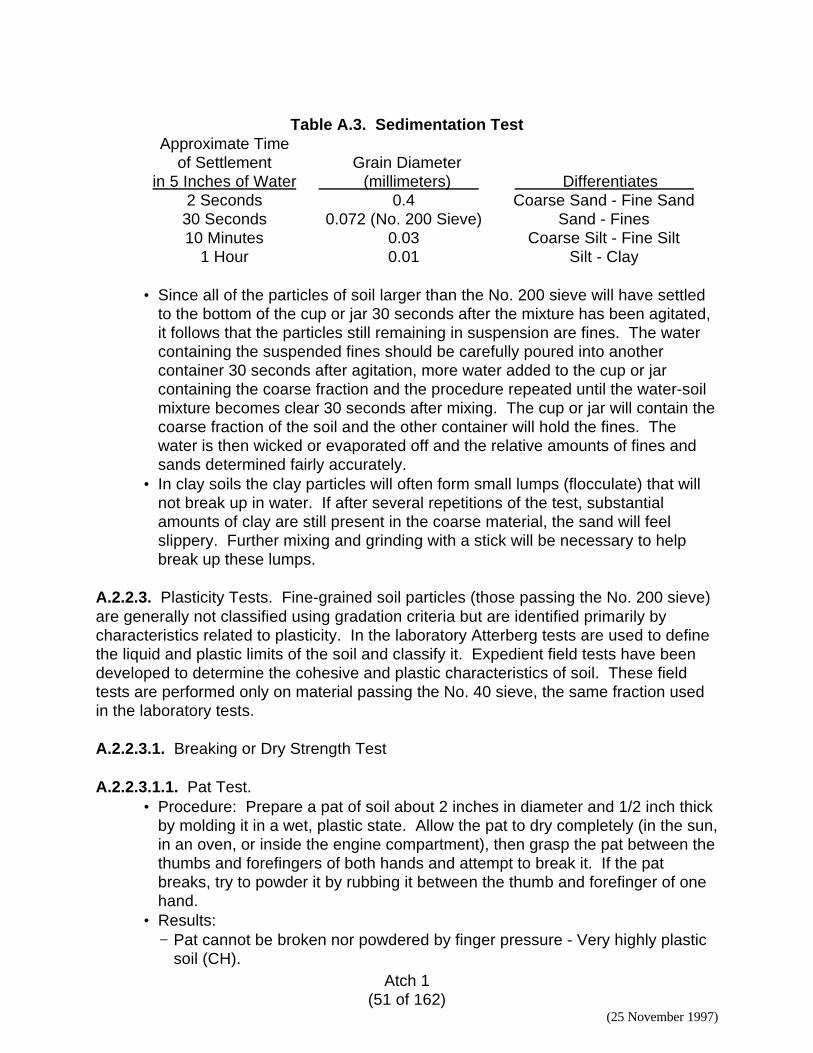
Atch 1(51 of 162)
(25 November 1997)
Table A.3. Sedimentation TestApproximate Time
of Settlementin 5 Inches of Water
Grain Diameter (millimeters) Differentiates
2 Seconds 0.4 Coarse Sand - Fine Sand30 Seconds 0.072 (No. 200 Sieve) Sand - Fines10 Minutes 0.03 Coarse Silt - Fine Silt
1 Hour 0.01 Silt - Clay
• Since all of the particles of soil larger than the No. 200 sieve will have settledto the bottom of the cup or jar 30 seconds after the mixture has been agitated,it follows that the particles still remaining in suspension are fines. The watercontaining the suspended fines should be carefully poured into anothercontainer 30 seconds after agitation, more water added to the cup or jarcontaining the coarse fraction and the procedure repeated until the water-soilmixture becomes clear 30 seconds after mixing. The cup or jar will contain thecoarse fraction of the soil and the other container will hold the fines. Thewater is then wicked or evaporated off and the relative amounts of fines andsands determined fairly accurately.
• In clay soils the clay particles will often form small lumps (flocculate) that willnot break up in water. If after several repetitions of the test, substantialamounts of clay are still present in the coarse material, the sand will feelslippery. Further mixing and grinding with a stick will be necessary to helpbreak up these lumps.
A.2.2.3. Plasticity Tests. Fine-grained soil particles (those passing the No. 200 sieve)are generally not classified using gradation criteria but are identified primarily bycharacteristics related to plasticity. In the laboratory Atterberg tests are used to definethe liquid and plastic limits of the soil and classify it. Expedient field tests have beendeveloped to determine the cohesive and plastic characteristics of soil. These fieldtests are performed only on material passing the No. 40 sieve, the same fraction usedin the laboratory tests.
A.2.2.3.1. Breaking or Dry Strength Test
A.2.2.3.1.1. Pat Test.• Procedure: Prepare a pat of soil about 2 inches in diameter and 1/2 inch thick
by molding it in a wet, plastic state. Allow the pat to dry completely (in the sun,in an oven, or inside the engine compartment), then grasp the pat between thethumbs and forefingers of both hands and attempt to break it. If the patbreaks, try to powder it by rubbing it between the thumb and forefinger of onehand.
• Results:− Pat cannot be broken nor powdered by finger pressure - Very highly plastic
soil (CH).
Atch 1(52 of 162)
(25 November 1997)
− Pat can be broken with great effort, but cannot be powdered - Highly plasticsoil (CL).
− Pat can be broken and powdered, but with some effort - Medium plastic soil(CL).
− Pat breaks easily and powders readily - Slightly plastic soil (ML, MH, or CL).− Pat has little or no dry strength and crumbles or powders when picked up -
Nonplastic soil (ML or MH) or (OL or OH).
Note: Dry pats of highly plastic clays often display shrinkage cracks. Breaking the patalong such a crack may not give a true indication of the strength. It is important todistinguish between a break along such a crack and a clean, fresh break that indicatesthe true dry strength of the soil.
A.2.2.3.1.2. Ball Test (Alternative to Pat Test).• Procedure: Select enough material to mold into a ball about one inch in
diameter. Mold the material until it has the consistency of putty, adding waterif necessary. From the molded material, make at three test specimens, 1/2inch diameter balls. Allow the test specimens to dry in the air, sun or byartificial means, as long as the temperature does not exceed 60 degrees C.Test the strength of the material by crushing between the fingers.
• Results:− No strength. The dry specimen crumbles into powder with mere pressure of
handling. (ML).− Low strength. The dry specimen crumbles into powder with some finger
pressure. (ML or MH).− Medium strength. The dry specimen breaks into pieces or crumbles with
considerable finger pressure. (MH or CL).− High strength. The dry specimen cannot be broken with finger pressure, but
will break into pieces between the thumb and a hard surface. (CL or CH).− Very High strength. The dry specimen cannot be broken between the thumb
and a hard surface. (CH).
Note: Natural dry lumps about 1/2 inch in diameter may be used, but do not use theresults if any of the lumps contain particles of coarse sand. The presence of highlycementitious materials in the soil such as calcium carbonate may produce exceptionallyhigh strengths.
A.2.2.3.2. Roll or Thread Test.• Procedure: A representative portion of the sample is mixed with water until it
can be molded or shaped without sticking to the fingers. This moisture contentis referred to as being just below the sticky limit. Prepare a nonabsorbentrolling surface by placing a sheet of glass or heavy wax paper on a flat or levelsupport, then shape the sample into an elongated cylinder and roll theprepared soil cylinder on the surface rapidly into a thread approximately 1/8inch in diameter. If the moist soil rolls into a thread, it has some plasticity.
Atch 1(53 of 162)
(25 November 1997)
The number of times it can be rolled into a thread without crumbling is ameasure of the degree of plasticity. Soils that cannot be rolled are nonplastic.
• Results:− Soil may be molded into a ball or cylinder and deformed under very firm
finger pressure without crumbling or cracking - High plasticity (CH).− Soil may be molded, but it cracks or crumbles under finger pressure -
Medium plasticity (CL).− Soil cannot be lumped into a ball or cylinder without breaking up - Low
plasticity (CL, ML, or MH).− Soil forms a soft, spongy ball or thread when molded - Organic material (OL
or OH).− Soil cannot be rolled into a thread at any moisture content - Nonplastic soil
(ML or MH).− The higher the soil is on the plasticity chart, the stiffer the threads are as
they dry out and the tougher the lumps are if the soil is remolded afterrolling.
Note: Micaceous silts and sands can be rolled due to the flaky nature of the mica. Thewet shaking test is the only way to distinguish this property.
A.2.2.3.3. Ribbon Test.• Procedure: Prepare a soil sample as in the roll or thread test. Form a roll of
soil about 1/2 to 3/4 inch in diameter and 3 to 5 inches long. Lay the rollacross the palm of one hand (palm up), and starting at one end, squeeze theroll between the thumb and forefinger over the edge of the hand to form a flatunbroken ribbon about 1/8 to 1/4 inch thick. Allow the ribbon as formed tohang free and unsupported. Continue squeezing and handling the rollcarefully to form the maximum length of ribbon that can be supported only bythe cohesive properties of the soil.
• Results:− Sample holds together for a length of 8 to 10 inches without breaking -
Highly plastic and highly compressive (CH).− Soil can be ribboned only with difficulty to 3 to 8 inch lengths - Low plasticity
(CL).
A.2.2.3.4. Wet Shaking Test.• Procedure:
− Form a ball of soil about 3/4 inch in diameter, moistened with water to justbelow the sticky limit. Smooth the soil pat in the palm of the hand with aknife blade or small spatula, shake it horizontally, and strike the back of thehand vigorously against the other hand. When shaking, water comes to thesurface of the sample producing a smooth, shiny, or livery appearance.
− Squeeze the sample between the thumb and forefinger of the other hand.The surface water will disappear. The surface will become dull and the
Atch 1(54 of 162)
(25 November 1997)
sample will become firm, resisting deformation. Cracks will occur aspressure is continued and the sample will crumble.
− If the water content is still adequate, shaking the broken pieces will causethem to liquefy again and flow together.
• Results: This process can only occur when the soil grains are bulky andnoncohesive. Very fine sands and silts are readily identified by this test. Evensmall amounts of clay will tend to retard the reaction to this test.− A rapid reaction is typical of nonplastic, fine sands and silts.− A sluggish reaction indicates slight plasticity indicating the silt has small
amounts of clay or organic silts.− No reaction at all does not indicate a complete absence of silt or fine sand.
A.2.2.3.5. Bite or Grit Test.• Procedure: Grind a small pinch of soil lightly between the teeth.• Results:
− Sandy soils. The sharp hard particles of even fine sands will grate veryharshly between the teeth and will be highly objectionable.
− Silty soils. Silt grains are not particularly gritty, but their presence is stillquite unpleasant and easily detected.
− Clayey soils. Clay grains feel smooth and powdery like flour. Dry lumps willstick when lightly touched with the tongue.
A.2.2.3.6. Shine Test.• Procedure: Rub a clay sample with a fingernail or smooth metal surface such
as a knife blade.• Results:
− Highly plastic clay will produce a definite shine.− Lean clays will remain dull.
A.2.2.3.7. Feel Test.• Consistency. Squeeze a piece of undisturbed soil between the thumb and
forefinger. It may be hard, stiff, brittle, friable, sticky, plastic, or soft. Remoldthe soil by working it between the hands. This can indicate the natural watercontent. Clays which become fluid on remolding are probably near their liquidlimit. If they remain stiff and crumble, they are probably below their liquid limit.
• Texture. Rub a portion of fine-grained soil between the fingers or on a moresensitive area such as the inside of the wrist. Results are similar to the bite orgrit test.
Atch 1(55 of 162)
(25 November 1997)
APPENDIX B
Condition Survey and Maintenance Procedures
B.1. Condition Survey Procedure
B.1.1. Introduction. During contingency or expedient operations, it is important thatpersonnel have the ability and tools to quickly and accurately assess a pre-existing ornewly constructed unsurfaced airfield and to monitor it for required maintenance. Thisrating system will show you how to divide the airfield into features (runway, taxiway,apron, hammerhead, and overruns) and sections, identify the distresses (problems)that exist or develop, rate the severity of each distress, and determine whether theairfield is operational or should be closed for repairs.
B.1.2. Equipment Required: Measuring wheel or 100-foot steel tape, carpenter’s6-foot folding rule, straightedge (8-foot 2´4 or other), stringline (if enough personnel areavailable), clipboard, inspection sheets, this appendix, and pens or pencils.
B.1.3. How the Method Works. The method for rating the condition of semi-preparedairfields has four steps:
Step 1: Divide the airfield into features and sections.Step 2: Inspect the airfield and identify the distresses.Step 3: Calculate the rating for each section.Step 4: Use the ratings to determine if the airfield is
GREEN • Operational for low-risk operations
AMBER • Needs monitoring and should be repaired if possible;medium-risk operations
RED • Dangerous and must be repaired; high-risk operations
When the surface condition is rated as amber, maintenance should be performed asthe mission allows. If any single distress is rated as red, the landing zone safety officerwill determine the feasibility of each operation.
Inspections should increase in frequency as the condition of the airfield degrades. Ifthe condition approaches red, inspection could be as frequent as before eachoperation.
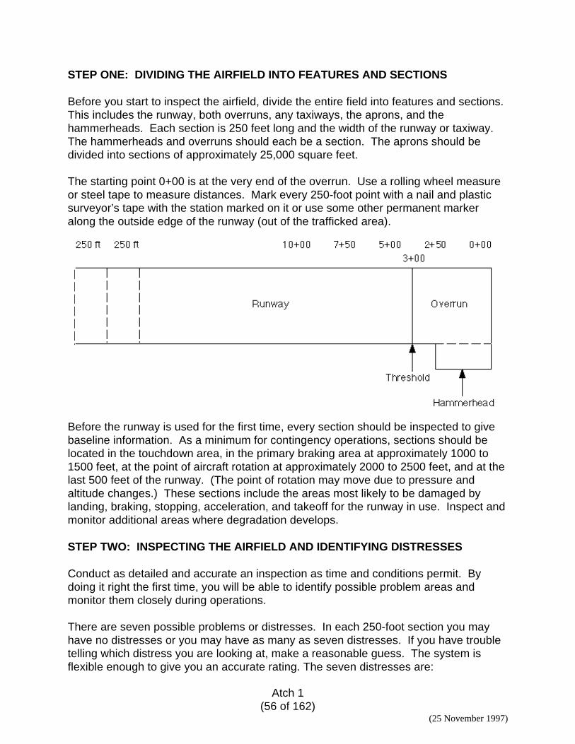
Atch 1(56 of 162)
(25 November 1997)
STEP ONE: DIVIDING THE AIRFIELD INTO FEATURES AND SECTIONS
Before you start to inspect the airfield, divide the entire field into features and sections.This includes the runway, both overruns, any taxiways, the aprons, and thehammerheads. Each section is 250 feet long and the width of the runway or taxiway.The hammerheads and overruns should each be a section. The aprons should bedivided into sections of approximately 25,000 square feet.
The starting point 0+00 is at the very end of the overrun. Use a rolling wheel measureor steel tape to measure distances. Mark every 250-foot point with a nail and plasticsurveyor’s tape with the station marked on it or use some other permanent markeralong the outside edge of the runway (out of the trafficked area).
Before the runway is used for the first time, every section should be inspected to givebaseline information. As a minimum for contingency operations, sections should belocated in the touchdown area, in the primary braking area at approximately 1000 to1500 feet, at the point of aircraft rotation at approximately 2000 to 2500 feet, and at thelast 500 feet of the runway. (The point of rotation may move due to pressure andaltitude changes.) These sections include the areas most likely to be damaged bylanding, braking, stopping, acceleration, and takeoff for the runway in use. Inspect andmonitor additional areas where degradation develops.
STEP TWO: INSPECTING THE AIRFIELD AND IDENTIFYING DISTRESSES
Conduct as detailed and accurate an inspection as time and conditions permit. Bydoing it right the first time, you will be able to identify possible problem areas andmonitor them closely during operations.
There are seven possible problems or distresses. In each 250-foot section you mayhave no distresses or you may have as many as seven distresses. If you have troubletelling which distress you are looking at, make a reasonable guess. The system isflexible enough to give you an accurate rating. The seven distresses are:

Atch 1(57 of 162)
(25 November 1997)
91. Potholes92. Ruts93. Loose aggregate94. Dust95. Rolling resistant material96. Jet blast erosion97. Stabilized layer failure
(The numbers 91–97 are associated with the Micro-Paver Pavement ManagementSystem and will be used in the computerized version of this system.)
Fill in the identifying information on the top of the inspection sheet and record theseverity levels on the table. The following pages will give you the definition of eachdistress and explain how to determine the severity level for that distress.
Unless otherwise stated, the distress severity measurements for contingency andtraining operations are the same.
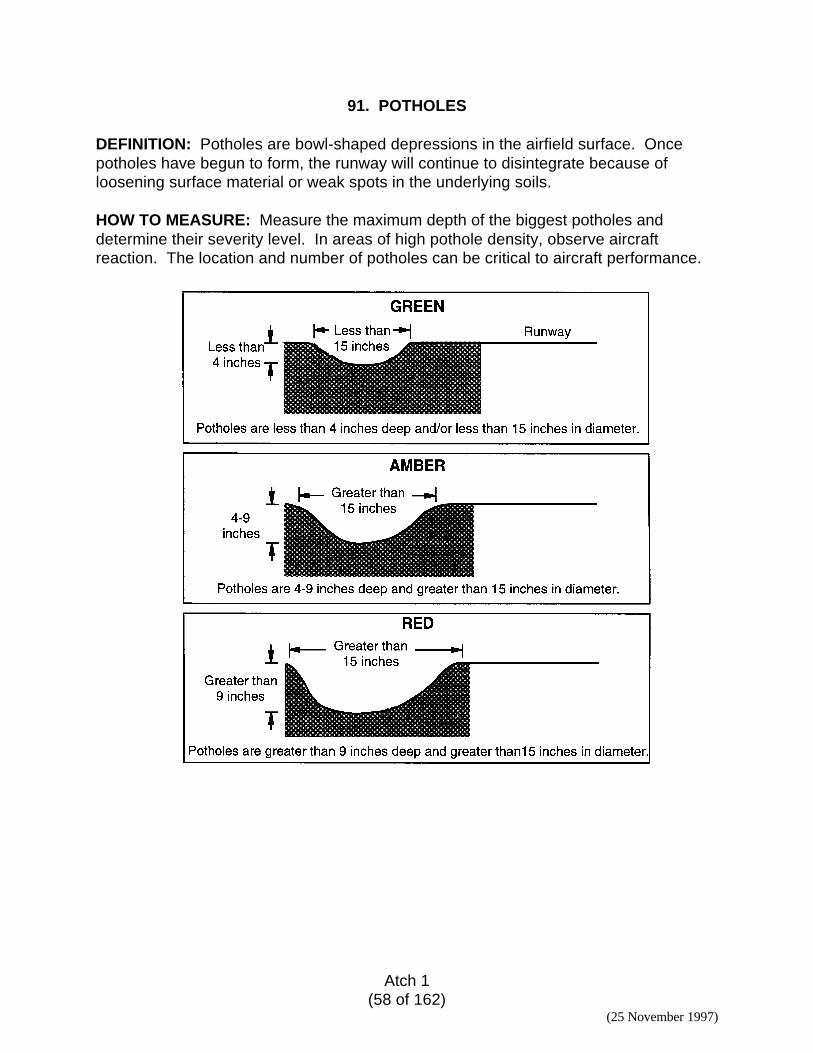
Atch 1(58 of 162)
(25 November 1997)
91. POTHOLES
DEFINITION: Potholes are bowl-shaped depressions in the airfield surface. Oncepotholes have begun to form, the runway will continue to disintegrate because ofloosening surface material or weak spots in the underlying soils.
HOW TO MEASURE: Measure the maximum depth of the biggest potholes anddetermine their severity level. In areas of high pothole density, observe aircraftreaction. The location and number of potholes can be critical to aircraft performance.
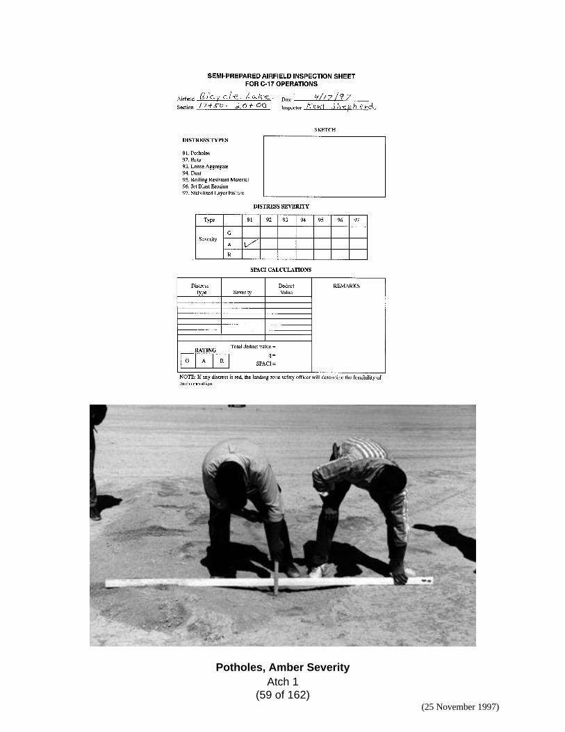
Atch 1(59 of 162)
(25 November 1997)
Potholes, Amber Severity
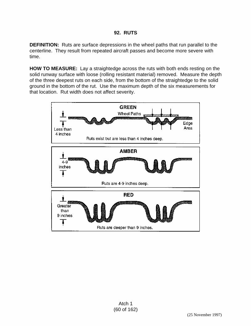
Atch 1(60 of 162)
(25 November 1997)
92. RUTS
DEFINITION: Ruts are surface depressions in the wheel paths that run parallel to thecenterline. They result from repeated aircraft passes and become more severe withtime.
HOW TO MEASURE: Lay a straightedge across the ruts with both ends resting on thesolid runway surface with loose (rolling resistant material) removed. Measure the depthof the three deepest ruts on each side, from the bottom of the straightedge to the solidground in the bottom of the rut. Use the maximum depth of the six measurements forthat location. Rut width does not affect severity.
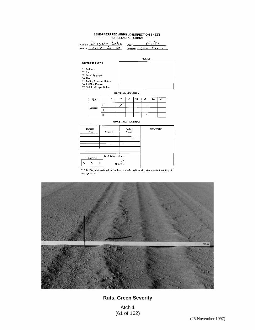
Atch 1(61 of 162)
(25 November 1997)
Ruts, Green Severity
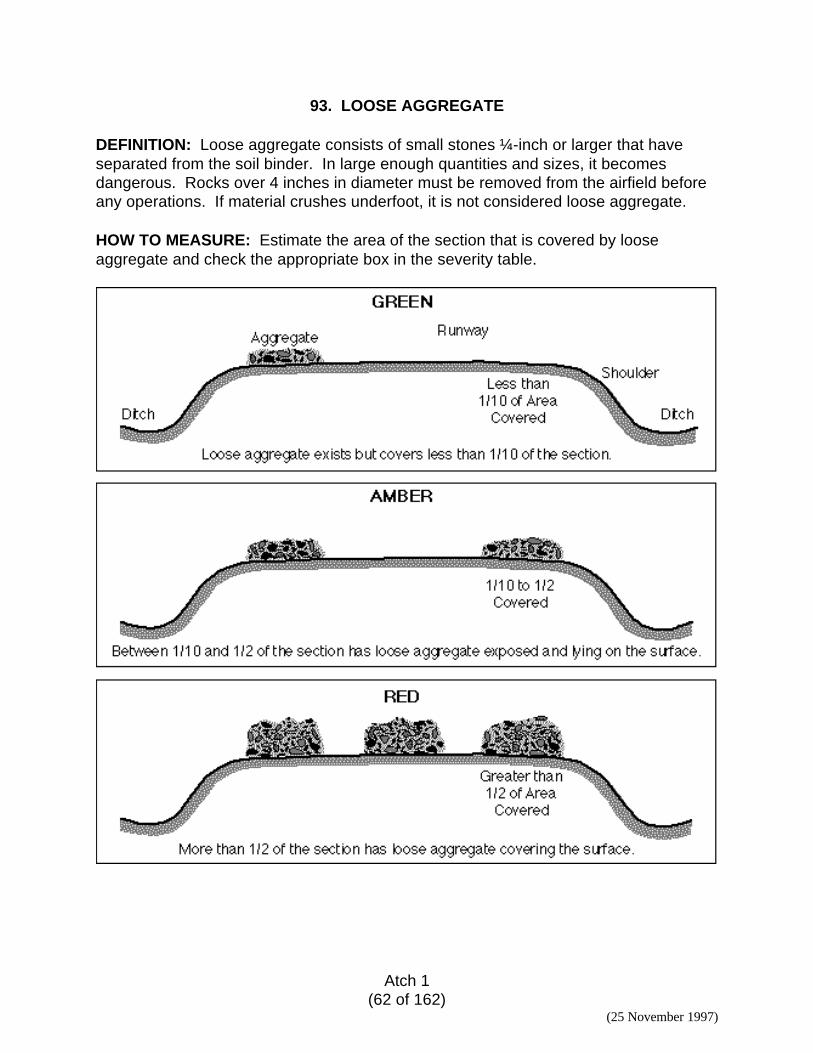
Atch 1(62 of 162)
(25 November 1997)
93. LOOSE AGGREGATE
DEFINITION: Loose aggregate consists of small stones ¼-inch or larger that haveseparated from the soil binder. In large enough quantities and sizes, it becomesdangerous. Rocks over 4 inches in diameter must be removed from the airfield beforeany operations. If material crushes underfoot, it is not considered loose aggregate.
HOW TO MEASURE: Estimate the area of the section that is covered by looseaggregate and check the appropriate box in the severity table.
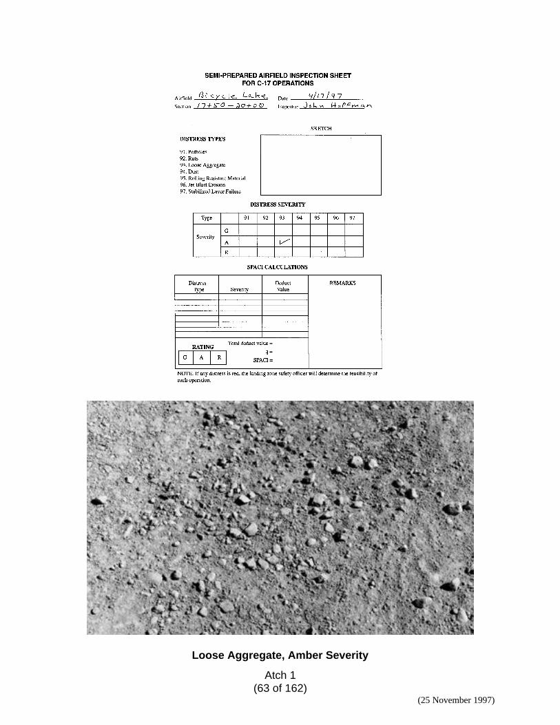
Atch 1(63 of 162)
(25 November 1997)
Loose Aggregate, Amber Severity
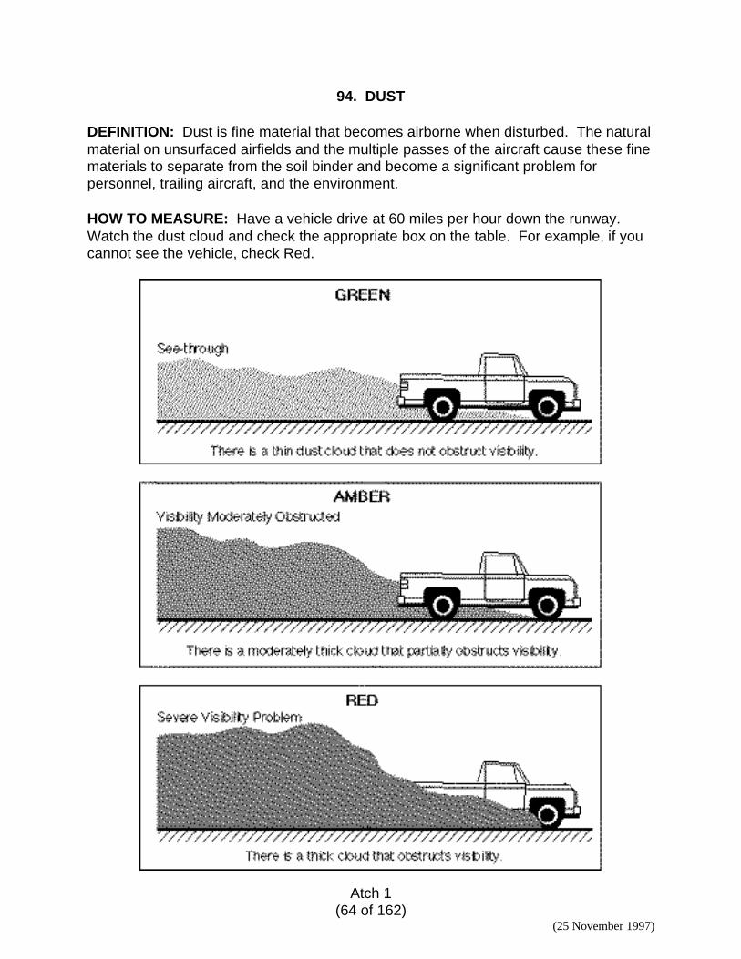
Atch 1(64 of 162)
(25 November 1997)
94. DUST
DEFINITION: Dust is fine material that becomes airborne when disturbed. The naturalmaterial on unsurfaced airfields and the multiple passes of the aircraft cause these finematerials to separate from the soil binder and become a significant problem forpersonnel, trailing aircraft, and the environment.
HOW TO MEASURE: Have a vehicle drive at 60 miles per hour down the runway.Watch the dust cloud and check the appropriate box on the table. For example, if youcannot see the vehicle, check Red.
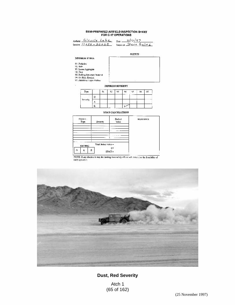
Atch 1(65 of 162)
(25 November 1997)
Dust, Red Severity
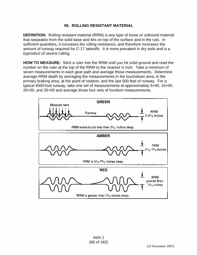
Atch 1(66 of 162)
(25 November 1997)
95. ROLLING RESISTANT MATERIAL
DEFINITION: Rolling resistant material (RRM) is any type of loose or unbound materialthat separates from the solid base and lies on top of the surface and in the ruts. Insufficient quantities, it increases the rolling resistance, and therefore increases theamount of runway required for C-17 takeoffs. It is more prevalent in dry soils and is abyproduct of severe rutting.
HOW TO MEASURE: Stick a ruler into the RRM until you hit solid ground and read thenumber on the ruler at the top of the RRM to the nearest ¼ inch. Take a minimum ofseven measurements in each gear path and average those measurements. Determineaverage RRM depth by averaging the measurements in the touchdown area, in theprimary braking area, at the point of rotation, and the last 500 feet of runway. For atypical 4000-foot runway, take one set of measurements at approximately 5+00, 10+00,20+00, and 35+00 and average those four sets of fourteen measurements.
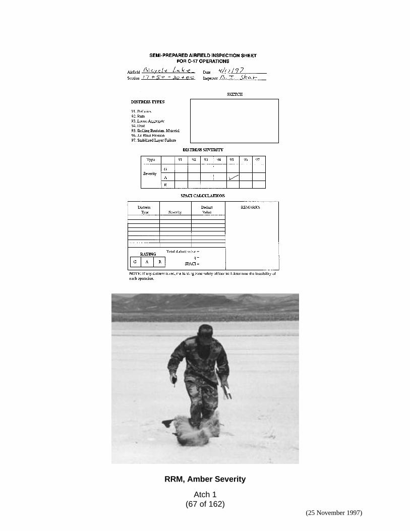
Atch 1(67 of 162)
(25 November 1997)
RRM, Amber Severity
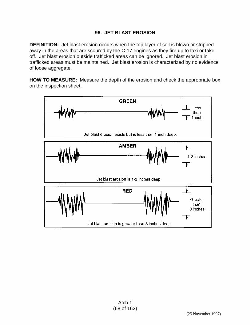
Atch 1(68 of 162)
(25 November 1997)
96. JET BLAST EROSION
DEFINITION: Jet blast erosion occurs when the top layer of soil is blown or strippedaway in the areas that are scoured by the C-17 engines as they fire up to taxi or takeoff. Jet blast erosion outside trafficked areas can be ignored. Jet blast erosion intrafficked areas must be maintained. Jet blast erosion is characterized by no evidenceof loose aggregate.
HOW TO MEASURE: Measure the depth of the erosion and check the appropriate boxon the inspection sheet.
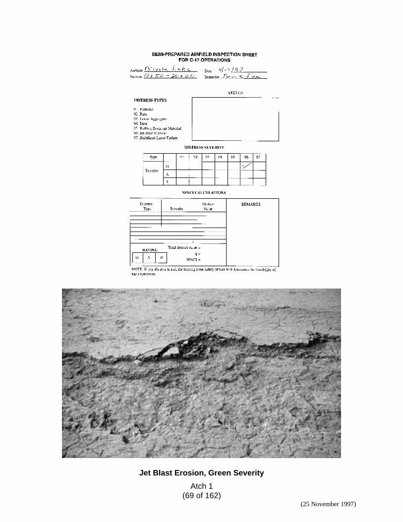
Atch 1(69 of 162)
(25 November 1997)
Jet Blast Erosion, Green Severity
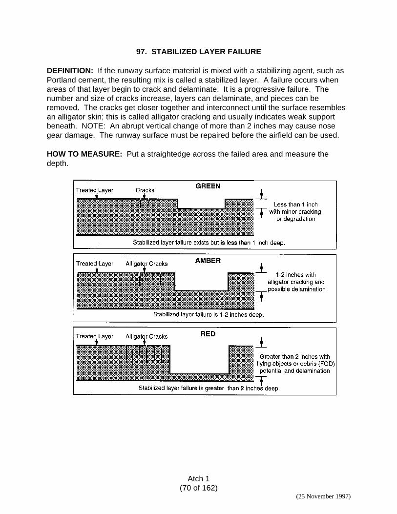
Atch 1(70 of 162)
(25 November 1997)
97. STABILIZED LAYER FAILURE
DEFINITION: If the runway surface material is mixed with a stabilizing agent, such asPortland cement, the resulting mix is called a stabilized layer. A failure occurs whenareas of that layer begin to crack and delaminate. It is a progressive failure. Thenumber and size of cracks increase, layers can delaminate, and pieces can beremoved. The cracks get closer together and interconnect until the surface resemblesan alligator skin; this is called alligator cracking and usually indicates weak supportbeneath. NOTE: An abrupt vertical change of more than 2 inches may cause nosegear damage. The runway surface must be repaired before the airfield can be used.
HOW TO MEASURE: Put a straightedge across the failed area and measure thedepth.
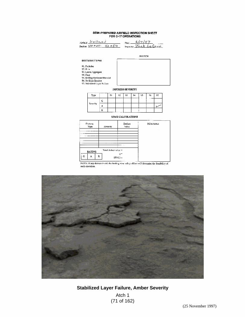
Atch 1(71 of 162)
(25 November 1997)
Stabilized Layer Failure, Amber Severity
Atch 1(72 of 162)
(25 November 1997)
STEP THREE: CALCULATING THE RATINGS
The distress measurements are used to calculate the Semi-Prepared Airfield ConditionIndex (SPACI), based on deduct values. A deduct value is a number from 0 to 100,with 0 meaning that the distress has no impact on the airfield condition and 100meaning that the airfield has completely failed. Deduct values for runways andtaxiways where the aircraft is moving are different than those on aprons andhammerheads where the C-17 may be offloading equipment. The deduct value tablereflects these differences. We will show how to do this calculation by running throughan example.
1. Fill in the identifying information at the top of the inspection sheet.
2. Put a check mark in the severity box corresponding to the distresses you find. Ifyou don’t find some distresses, leave those boxes blank.
3. Refer to the “Table of Deduct Values for C-17 Operations ” on page 77. Eachdistress has a deduct value for each severity level.
4. For potholes of Green severity on the runway, the deduct value is 4.
5. Record that number in the correct box on the bottom left side of the inspectionsheet.
6. For ruts at Amber severity, the deduct value is 18.
7. For loose aggregate at Amber severity, the deduct value is 6.
8. For dust at Amber severity, the deduct value is 4.
9. Add all the distress values and record the total on the line labeled “Total deductvalue.” In this case, the total deduct value is 32.
10. Count the total number of distresses that have deduct values greater than 5.That is the q value. Record it on the line labeled q. For this example, q is 2.
11. On the SPACI curve (page 77), locate the “Total Deduct Value.” Go across thenumbers on the bottom of the graph until you reach the total deduct value of 32.
12. Go up the vertical line until it intersects with the curved line that matches your qnumber (in this example, 2). From that point, follow the line across to the left tofind the rating (the SPACI). For this example, the SPACI is 77.
13. Go to the SPACI scale (page 77), which shows that 77 is in the Green range.
14. Circle this overall rating on the bottom left of the inspection sheet.
15. This is the rating for this section. The rating for the runway is the average of theratings from all the sections. For example, SPACIs of 63, 59 and 67 in differentsections would give an average SPACI of 63 for the whole runway.
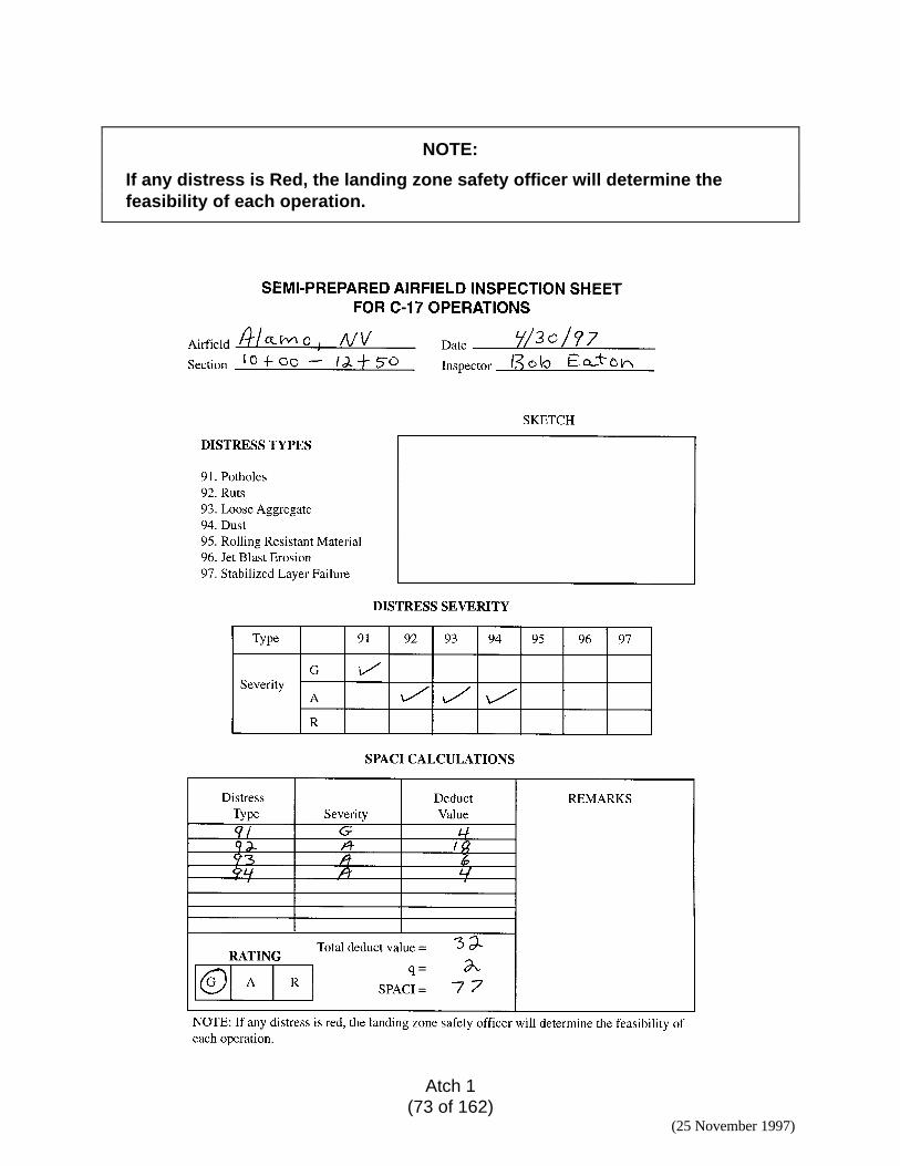
Atch 1(73 of 162)
(25 November 1997)
NOTE:
If any distress is Red, the landing zone safety officer will determine thefeasibility of each operation.
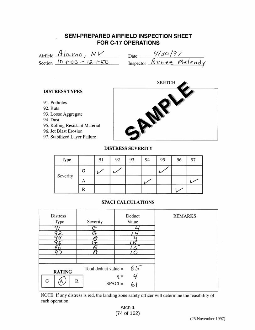
Atch 1(74 of 162)
(25 November 1997)

Atch 1(75 of 162)
(25 November 1997)
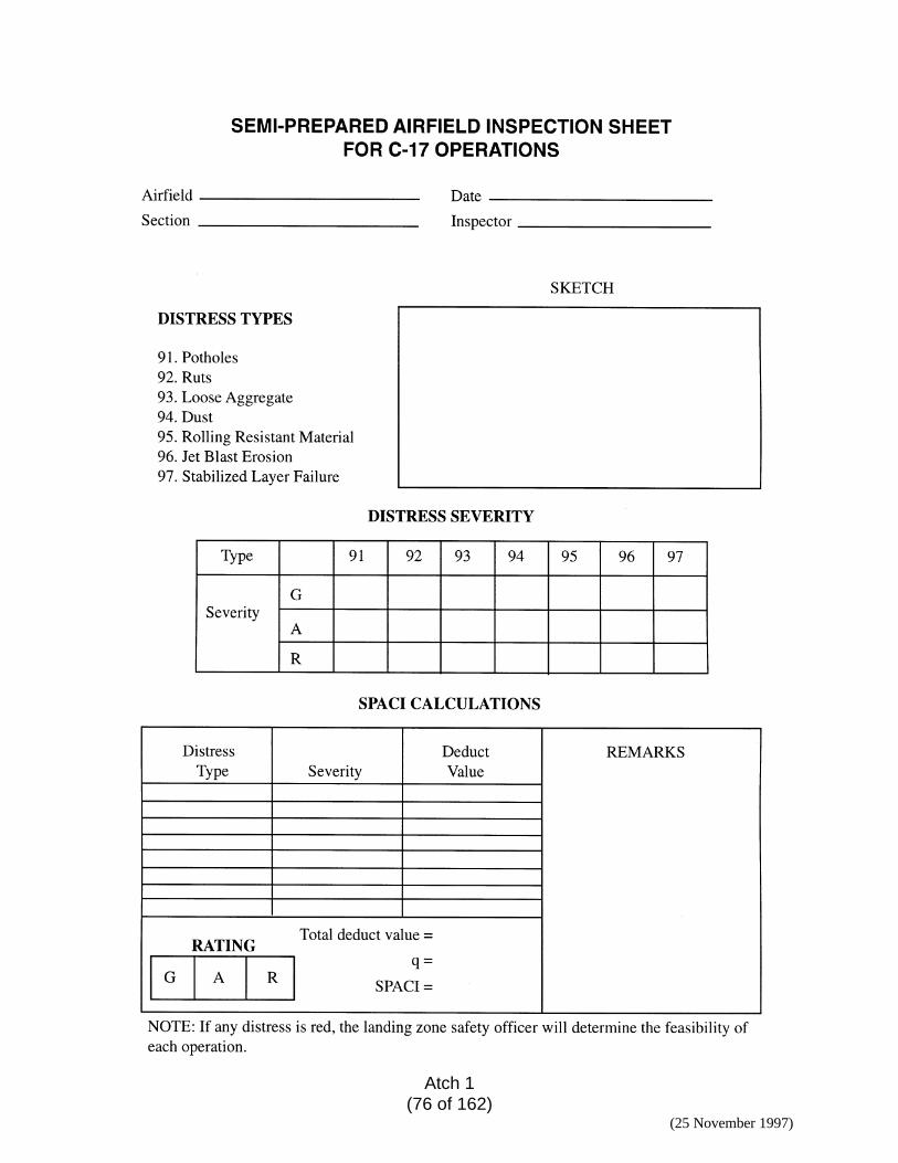
Atch 1(76 of 162)
(25 November 1997)
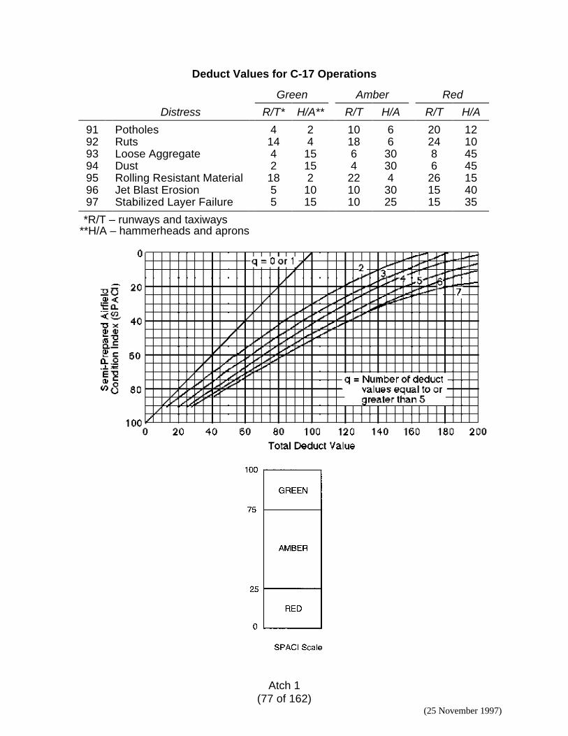
Atch 1(77 of 162)
(25 November 1997)
Deduct Values for C-17 Operations
Green Amber Red
Distress R/T* H/A** R/T H/A R/T H/A
91 Potholes 4 2 10 6 20 1292 Ruts 14 4 18 6 24 1093 Loose Aggregate 4 15 6 30 8 4594 Dust 2 15 4 30 6 4595 Rolling Resistant Material 18 2 22 4 26 1596 Jet Blast Erosion 5 10 10 30 15 4097 Stabilized Layer Failure 5 15 10 25 15 35
*R/T – runways and taxiways**H/A – hammerheads and aprons
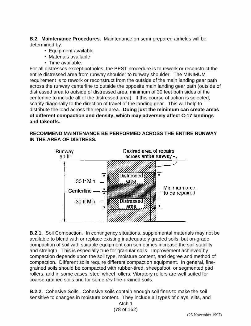
Atch 1(78 of 162)
(25 November 1997)
B.2. Maintenance Procedures. Maintenance on semi-prepared airfields will bedetermined by:
• Equipment available• Materials available• Time available.
For all distresses except potholes, the BEST procedure is to rework or reconstruct theentire distressed area from runway shoulder to runway shoulder. The MINIMUMrequirement is to rework or reconstruct from the outside of the main landing gear pathacross the runway centerline to outside the opposite main landing gear path (outside ofdistressed area to outside of distressed area, minimum of 30 feet both sides of thecenterline to include all of the distressed area). If this course of action is selected,scarify diagonally to the direction of travel of the landing gear. This will help todistribute the load across the repair area. Doing just the minimum can create areasof different compaction and density, which may adversely affect C-17 landingsand takeoffs.
RECOMMEND MAINTENANCE BE PERFORMED ACROSS THE ENTIRE RUNWAYIN THE AREA OF DISTRESS.
B.2.1. Soil Compaction. In contingency situations, supplemental materials may not beavailable to blend with or replace existing inadequately graded soils, but on-gradecompaction of soil with suitable equipment can sometimes increase the soil stabilityand strength. This is especially true for granular soils. Improvement achieved bycompaction depends upon the soil type, moisture content, and degree and method ofcompaction. Different soils require different compaction equipment. In general, fine-grained soils should be compacted with rubber-tired, sheepsfoot, or segmented padrollers, and in some cases, steel wheel rollers. Vibratory rollers are well suited forcoarse-grained soils and for some dry fine-grained soils.
B.2.2. Cohesive Soils. Cohesive soils contain enough soil fines to make the soilsensitive to changes in moisture content. They include all types of clays, silts, and
Atch 1(79 of 162)
(25 November 1997)
clayey and silty sands and gravels, such as CH, CL, MH, ML, SC, SM, GC, and GM.For a given compactive effort and method of compaction, there is an optimum moisturecontent which results in the maximum dry density of the soil. At any other moisturecontent, the resulting soil dry density will be less for the same compactive effort.Compact cohesive soils at or slightly higher than the optimum moisture content, exceptwhen using a vibratory roller. Rubber-tired and sheepsfoot rollers are most effective forcompacting cohesive soils. A towed sheepsfoot with a contact pressure of 400–600 psior a 35- to 50-ton rubber-tired roller with four wheels will usually yield satisfactoryresults. Vibratory rollers are effective on some cohesive soils, particularly thosecontaining granular fractions such as SC, SM, GC, and GM. Use steel wheel rollers toseal the surface of cohesive soils to decrease rainfall penetration.
B.2.3. Cohesionless Soils. These soils are relatively clean sands and gravels, nothighly moisture sensitive and relatively pervious. They include SW, SP, GW, and GPsoil types. Optimum moisture content and maximum dry density may need to beconsidered depending upon the type and quantity of soil fines. If a granular soilcontains essentially no fines, optimum density can be achieved when the soil is almostsaturated. Cohesionless soils often require continuous wetting during compaction toprevent bulking. These soils can be compacted most effectively by vibratory rollerswith a total drum force of 15–20 tons. Rubber-tired rollers are somewhat less effective.Steel wheel rollers are normally used to obtain a smooth finish surface.
B.2.4. Compaction Method. The choice of compaction equipment should depend uponsoil type and moisture content. Equipment should be tracked over the material at leastfour times, both parallel and perpendicular to the centerline of the runway. Traffickingshould continue until no further densification of the material can be observed. Ifadditional passes do not increase soil strength, the material is probably too dry or toowet. Pumping of the material in front of the roller also indicates the material is too wet.
B.2.5. Equipment Sizes. Sizes referenced in paragraphs B.2.2 and B.2.3 shouldprovide adequate compaction to depths of 6–9 inches. If the available compactionequipment is smaller, the soil must be compacted in thinner lifts with more passes, untilno further densification of the material can be observed on each lift.
B.2.6. Repairs. Passes should begin on the outside of the repair adjacent to theexisting adequate surface, and should proceed toward the center of the repair. Passesshould overlap, and the equipment should “crawl,” rather than race, across the surface.
B.2.7. Soil Testing. Where time or available equipment precludes moisture/densitytests to confirm compaction, dynamic cone penetrometer (DCP) tests should beperformed following compaction to determine if the material is strong enough to supportaircraft operations.
Atch 1(80 of 162)
(25 November 1997)
91. POTHOLES
1. Cut to at least 2 inches below the base of the pothole and at least 2feet around the hole.
2. Add material identical to the surrounding material. This is especiallyimportant if the soil is stabilized.
3. Wet as required to obtain the optimum water content.4. Compact to obtain the optimum density.5. Lift thickness may have to be reduced to 2- to 3-inch lifts to obtain the
optimum density depending on the compaction equipment available.
92. RUTS
1. Wet if dry.2. Scarify.3. Add material as required.4. Rewet if necessary.5. Grade to a proper cross-section.6. Rewet as required.7. Compact to a required optimum density.8. Repeat 5, 6, and 7 in 2- to 3-inch lifts if needed to achieve the
optimum density with the compaction equipment available.
93. LOOSE AGGREGATE
1. Wet if dry.2. Scarify if conditions are severe.3. Rewet as needed.4. Add material if necessary.5. Rescarify if material is added.6. Rewet as needed.7. Grade to a proper cross-section.8. Compact to the optimum density.9. Wet and compact again if necessary to obtain the optimum density
with the compaction equipment available.
94. DUST1. Wet as needed.2. Use a dust palliative.3. Stabilize if time and resources are available.4. Install matting if required by the mission.
Atch 1(81 of 162)
(25 November 1997)
95. ROLLING RESISTANT MATERIAL
1. Wet.2. Scarify.3. Rewet as needed.4. Grade to a proper cross-section.5. Rewet as needed.6. Compact to obtain the optimum density.7. Repeat 5 and 6 in lifts if necessary to obtain the optimum density with
the compaction equipment available.
96. JET BLAST EROSION
1. Wet if dry.2. Scarify to include the undisturbed area to ensure good adhesion or
bonding of the repair.3. Rewet and add material if necessary.4. Rescarify if material is added.5. Grade to a proper cross-section.6. Rewet as needed.7. Compact to obtain the optimum density.8. Repeat steps 6 and 7 if necessary to obtain the optimum density with
the compaction equipment available.
97. STABILIZED LAYER FAILURE
Procedure One1. Determine the stabilizing additive and amounts.2. Pulverize.3. Add material if necessary.4. Obtain optimum moisture content.5. Add the identical stabilizing additive.6. Mix the materials. Be sure to scarify at least 2 inches into the existing
stabilized material to achieve a proper cold joint both below andaround the repair area.
7. Grade to a proper cross-section.8. Add additional water if necessary to obtain optimum moisture content.9. Grade and compact, in lifts, to obtain the optimum density.*10. Check the cold joints for proper adhesion, with a pneumatic roller if
available.11. If failure is evident, repeat steps 6–10.
Procedure Two1. Remove all failed material.2. Mix up repair stabilized material on site.3. Follow procedure in TM 5-822-7, Appendix D, page D-11.
*See TM 5-822-7, Appendix D, page D-11 for specific guidance.
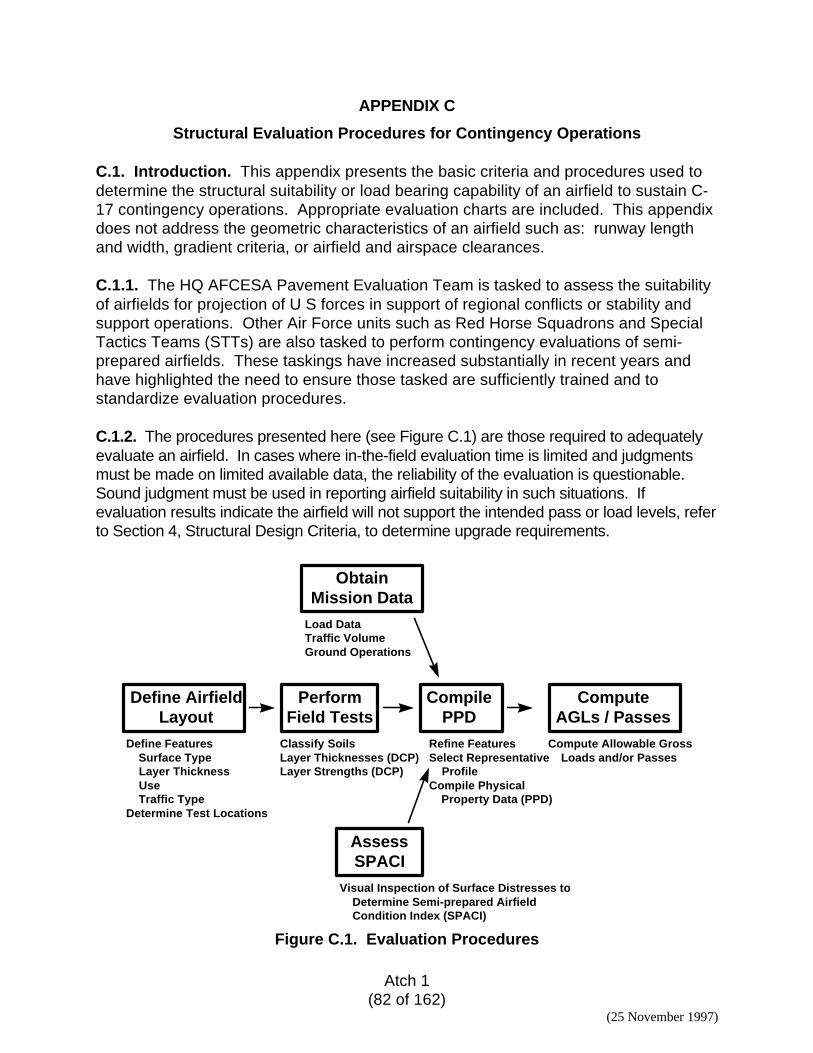
Atch 1(82 of 162)
(25 November 1997)
APPENDIX C
Structural Evaluation Procedures for Contingency Operations
C.1. Introduction. This appendix presents the basic criteria and procedures used todetermine the structural suitability or load bearing capability of an airfield to sustain C-17 contingency operations. Appropriate evaluation charts are included. This appendixdoes not address the geometric characteristics of an airfield such as: runway lengthand width, gradient criteria, or airfield and airspace clearances.
C.1.1. The HQ AFCESA Pavement Evaluation Team is tasked to assess the suitabilityof airfields for projection of U S forces in support of regional conflicts or stability andsupport operations. Other Air Force units such as Red Horse Squadrons and SpecialTactics Teams (STTs) are also tasked to perform contingency evaluations of semi-prepared airfields. These taskings have increased substantially in recent years andhave highlighted the need to ensure those tasked are sufficiently trained and tostandardize evaluation procedures.
C.1.2. The procedures presented here (see Figure C.1) are those required to adequatelyevaluate an airfield. In cases where in-the-field evaluation time is limited and judgmentsmust be made on limited available data, the reliability of the evaluation is questionable.Sound judgment must be used in reporting airfield suitability in such situations. Ifevaluation results indicate the airfield will not support the intended pass or load levels, referto Section 4, Structural Design Criteria, to determine upgrade requirements.
ObtainMission Data
Define AirfieldLayout
PerformField Tests
CompilePPD
ComputeAGLs / Passes
AssessSPACI
Load DataTraffic VolumeGround Operations
Visual Inspection of Surface Distresses to Determine Semi-prepared Airfield Condition Index (SPACI)
Define Features Surface Type Layer Thickness Use Traffic TypeDetermine Test Locations
Classify SoilsLayer Thicknesses (DCP)Layer Strengths (DCP)
Compute Allowable Gross Loads and/or Passes
Refine FeaturesSelect Representative ProfileCompile Physical Property Data (PPD)
Figure C.1. Evaluation Procedures
Atch 1(83 of 162)
(25 November 1997)
C.1.3. If questions arise in the field, one of the following should be contacted:
• HQ AFCESA/CESC139 Barnes Drive, Suite 1Tyndall AFB, FL 32403-5319
Mr James Greene, DSN 523-6334 Comm (850) 283-6334USAF Pavements Manager
Mr Richard Smith, DSN 523-6084 Comm (850) 283-6084Pavements Laboratory Manager
FAX DSN 523-6499 Comm (850) 283-6499
• CEWES-GP-NAirfields and Pavements DivisionGeotechnical LaboratoryU S Army Engineer Waterways Experiment Station3909 Halls Ferry RoadVicksburg, MS 39180-6199
Dr Albert Bush Comm (601) 634-3545 or 1-800-522-6937 ext 3545Mr Don Alexander Comm (601) 634-2731 or 1-800-522-6937 ext 2731
FAX Comm (601) 634-3020
C.2. Define Initial Airfield Layout
C.2.1. Make an initial tour of the airfield.
C.2.1.1. Verify dimensions of the airfield and accuracy of existing drawings if available.Existing information on the airfield such as: soil boring data; geological, topographical,and agricultural maps; and aerial photographs would also be helpful if available.
C.2.1.2. Use expedient methods to survey (taping, measuring wheel, or pacing).
C.2.1.3. Update existing plans or make new scaled drawing as required.
C.2.2. Divide the airfield pavement system into features based upon commoncharacteristics which are: the surface type, thickness, and construction history data;available subsurface layer data; use; and traffic type.
C.2.2.1. Surface Types:• AM-2 Mat• Gravel / Unsurfaced• Stabilized Material
Note: A specific feature contains only one surface type.
Atch 1(84 of 162)
(25 November 1997)
C.2.2.2. Surface Layer Thickness and Construction History Data. All surface materialin a specific feature must share a constant nominal thickness within reason and acommon construction history. Construction history is comprised of data regarding thematerials used and year of original construction, as well as all subsequent maintenanceand repair materials and techniques.
C.2.2.3. Subsurface Layers:• Types• Thicknesses• Strengths
C.2.2.4. Use:• R = Runway• O = Overrun• T = Taxiway• A = Apron
C.2.2.5. Traffic Type:• A = Channelized traffic, full design weight of aircraft (All areas of contingency
airfields should be evaluated as A traffic.)
C.2.3. Determine Test Locations. The numbers and locations of soil strength tests andsamples will vary with the type of airfield, size of airfield, proposed mission of theairfield, number of features, and time available for conducting the tests. Test locationsmust be chosen wisely and should accurately cover each feature or aspect of theairfield, yet may need to be minimized due to aircraft operations or time constraints.Soil conditions are extremely variable; therefore, as many tests as time andcircumstance will permit should be taken. The strength range and uniformity of thearea will control the number of tests required. In all cases it is advisable to testapparent weak areas first, since the weakest conditions control the pavementevaluation. In areas of doubtful strength or where evidences of changing layerstructure occur, the tests may be closely spaced. On the other hand, in areas wherethe structure appears to be firm and uniform, tests may be few and widely spaced.After weak areas have been tested, areas of high traffic intensity or loading such astake-off/touch-down zones, runway/taxiway intersections, and taxi lanes on apronsshould be tested. Figure C.2 shows recommended test locations for semi-preparedairfields. Conduct as many tests as possible in the time available.
C.3. Collect Field Data to Determine Airfield Structural Properties
C.3.1. Types.• Identify surface and any underlying base, subbase, and subgrade materials
using field identification methods and classify using the United SoilClassification System (USCS). See Appendix A.
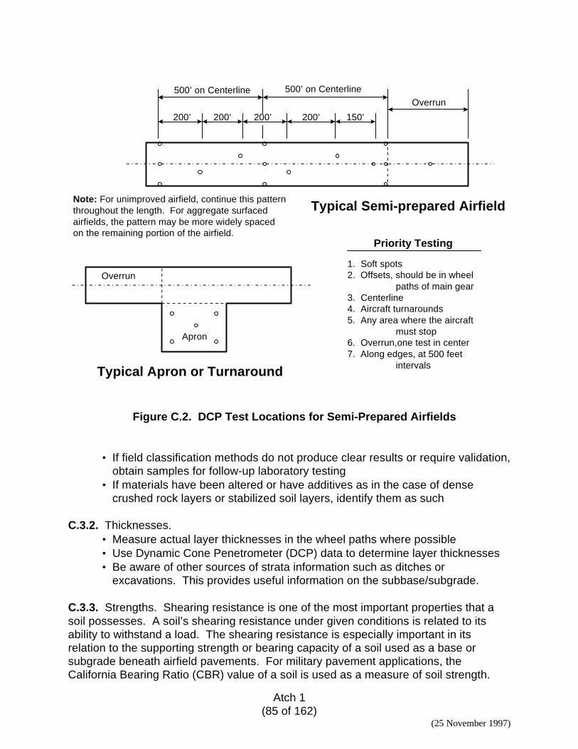
Atch 1(85 of 162)
(25 November 1997)
500’ on Centerline 500’ on CenterlineOverrun
200’200’ 200’200’ 150’
Note: For unimproved airfield, continue this patternthroughout the length. For aggregate surfacedairfields, the pattern may be more widely spacedon the remaining portion of the airfield.
Typical Semi-prepared Airfield
Priority Testing
1. Soft spots2. Offsets, should be in wheel
paths of main gear3. Centerline4. Aircraft turnarounds5. Any area where the aircraft
must stop6. Overrun,one test in center7. Along edges, at 500 feet
intervalsTypical Apron or Turnaround
Overrun
Apron
Figure C.2. DCP Test Locations for Semi-Prepared Airfields
• If field classification methods do not produce clear results or require validation,obtain samples for follow-up laboratory testing
• If materials have been altered or have additives as in the case of densecrushed rock layers or stabilized soil layers, identify them as such
C.3.2. Thicknesses.• Measure actual layer thicknesses in the wheel paths where possible• Use Dynamic Cone Penetrometer (DCP) data to determine layer thicknesses• Be aware of other sources of strata information such as ditches or
excavations. This provides useful information on the subbase/subgrade.
C.3.3. Strengths. Shearing resistance is one of the most important properties that asoil possesses. A soil’s shearing resistance under given conditions is related to itsability to withstand a load. The shearing resistance is especially important in itsrelation to the supporting strength or bearing capacity of a soil used as a base orsubgrade beneath airfield pavements. For military pavement applications, theCalifornia Bearing Ratio (CBR) value of a soil is used as a measure of soil strength.
Atch 1(86 of 162)
(25 November 1997)
Laboratory methods of determining CBR values are time consuming and thusimpractical for expedient or contingency evaluations. Several methods are available todetermine CBR values in the field.
• Dynamic Cone Penetrometer. The DCP is the preferred method ofobtaining CBR field data. It will penetrate layers having CBR strengths inexcess of 100 and will measure soil strengths less than 1. It is a powerful,relatively compact, sturdy device that produces consistent results. Its use willbe discussed in detail later in this section.
• Airfield Cone Penetrometer (ACP). The ACP is a probe-type instrument thatwhen pushed down through the soil gives an airfield index (AI) of soil strength.This AI can be correlated to CBR values. This instrument is commonly usedby USAF SSTs for expedient evaluations because of its portability andsimplicity to operate. Its range is limited to 0 to 18 CBR and it will notpenetrate many crusts, thin base course, or gravel materials. Consistency oftest results is also difficult due to variability of soil strengths that impact therate of penetration. Due to this and depth constraints, it is not recommendedfor C-17 evaluations.
• Electronic Cone Penetrometer (ECP). The contingency soils van operated byHQ AFCESA is equipped with an ECP that is hydraulically pushed through thesoil layers to depths of typically five to seven feet. The cone tip pressure ismeasured and recorded by the on-board computer system and is correlated toCBR values. Soil cohesion measurements are also recorded and used inconjunction with the tip pressure to assist in soil classification. This one-of-a-kind item is also equipped with a core drill capable of coring through flexibleand rigid pavement layers as required, is air-transportable by C-130, C-141,C-5, and C-17 aircraft, and provides accurate, consistent data. This van is notavailable nor appropriate for all contingency evaluations, but its use should beconsidered when other methods of data collection do not provide clear results.
• Field Small Aperture CBR Test. Standard CBR tests may also be performedon the surface or through core holes in the pavement surface. This use isnormally limited to tests on the surface of the base course. These tests maybe performed in conjunction with DCP tests to validate the data or as standalone tests in cases where use of the DCP is not applicable. These tests aredescribed in detail in FM 5-530/AFM 89-3.
• USCS Correlation. This is the quickest, yet least accurate method ofdetermining CBR values. For each soil type, empirical studies havedetermined a range of CBR values. These values are shown on the TableA.2, Soil Characteristics Chart in Appendix A. These CBR ranges are onlyestimates and due to the varying soil types and strengths encountered acrossan airfield, the lowest CBR values in the range should be used, and then withjudgment and caution.
C.3.3.1. Measure soil layer thickness and strengths using the DCP.
C.3.3.1.1. Description. The DCP consists of a 16-mm-diameter stainless steel rod witha cone attached to one end which is driven into the soil by means of an 8 kg sliding
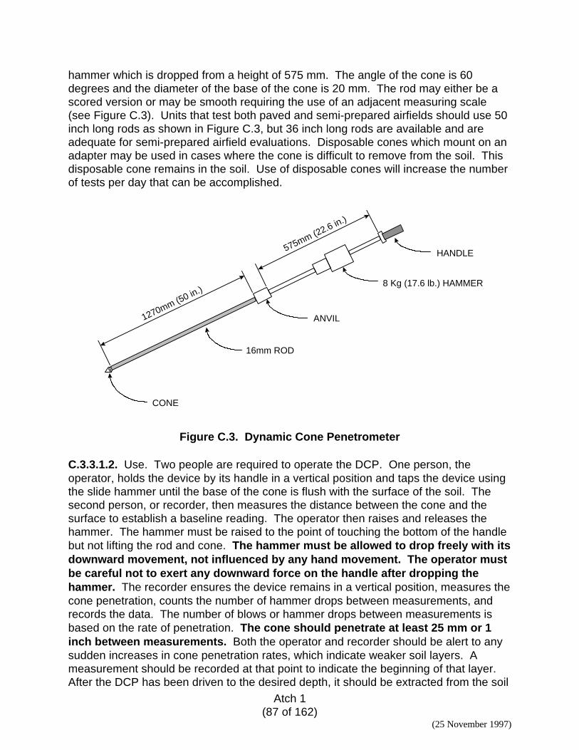
Atch 1(87 of 162)
(25 November 1997)
hammer which is dropped from a height of 575 mm. The angle of the cone is 60degrees and the diameter of the base of the cone is 20 mm. The rod may either be ascored version or may be smooth requiring the use of an adjacent measuring scale(see Figure C.3). Units that test both paved and semi-prepared airfields should use 50inch long rods as shown in Figure C.3, but 36 inch long rods are available and areadequate for semi-prepared airfield evaluations. Disposable cones which mount on anadapter may be used in cases where the cone is difficult to remove from the soil. Thisdisposable cone remains in the soil. Use of disposable cones will increase the numberof tests per day that can be accomplished.
1270mm (50 in.)
575mm (22.6 in.)
CONE
16mm ROD
ANVIL
8 Kg (17.6 lb.) HAMMER
HANDLE
Figure C.3. Dynamic Cone Penetrometer
C.3.3.1.2. Use. Two people are required to operate the DCP. One person, theoperator, holds the device by its handle in a vertical position and taps the device usingthe slide hammer until the base of the cone is flush with the surface of the soil. Thesecond person, or recorder, then measures the distance between the cone and thesurface to establish a baseline reading. The operator then raises and releases thehammer. The hammer must be raised to the point of touching the bottom of the handlebut not lifting the rod and cone. The hammer must be allowed to drop freely with itsdownward movement, not influenced by any hand movement. The operator mustbe careful not to exert any downward force on the handle after dropping thehammer. The recorder ensures the device remains in a vertical position, measures thecone penetration, counts the number of hammer drops between measurements, andrecords the data. The number of blows or hammer drops between measurements isbased on the rate of penetration. The cone should penetrate at least 25 mm or 1inch between measurements. Both the operator and recorder should be alert to anysudden increases in cone penetration rates, which indicate weaker soil layers. Ameasurement should be recorded at that point to indicate the beginning of that layer.After the DCP has been driven to the desired depth, it should be extracted from the soil
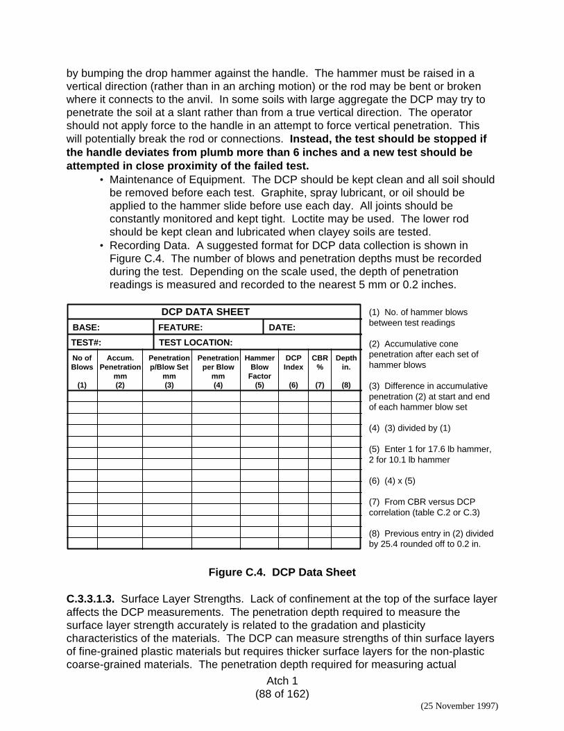
Atch 1(88 of 162)
(25 November 1997)
by bumping the drop hammer against the handle. The hammer must be raised in avertical direction (rather than in an arching motion) or the rod may be bent or brokenwhere it connects to the anvil. In some soils with large aggregate the DCP may try topenetrate the soil at a slant rather than from a true vertical direction. The operatorshould not apply force to the handle in an attempt to force vertical penetration. Thiswill potentially break the rod or connections. Instead, the test should be stopped ifthe handle deviates from plumb more than 6 inches and a new test should beattempted in close proximity of the failed test.
• Maintenance of Equipment. The DCP should be kept clean and all soil shouldbe removed before each test. Graphite, spray lubricant, or oil should beapplied to the hammer slide before use each day. All joints should beconstantly monitored and kept tight. Loctite may be used. The lower rodshould be kept clean and lubricated when clayey soils are tested.
• Recording Data. A suggested format for DCP data collection is shown inFigure C.4. The number of blows and penetration depths must be recordedduring the test. Depending on the scale used, the depth of penetrationreadings is measured and recorded to the nearest 5 mm or 0.2 inches.
DCP DATA SHEET
No ofBlows
(1)
Accum.Penetration
mm(2)
Penetrationp/Blow Set
mm(3)
Penetrationper Blow
mm(4)
HammerBlow
Factor(5)
DCPIndex
(6)
CBR%
(7)
Depthin.
(8)
BASE: DATE:
TEST#:
FEATURE:
TEST LOCATION:
(1) No. of hammer blowsbetween test readings
(2) Accumulative cone penetration after each set ofhammer blows
(3) Difference in accumulativepenetration (2) at start and endof each hammer blow set
(4) (3) divided by (1)
(5) Enter 1 for 17.6 lb hammer,2 for 10.1 lb hammer
(6) (4) x (5)
(7) From CBR versus DCPcorrelation (table C.2 or C.3)
(8) Previous entry in (2) dividedby 25.4 rounded off to 0.2 in.
Figure C.4. DCP Data Sheet
C.3.3.1.3. Surface Layer Strengths. Lack of confinement at the top of the surface layeraffects the DCP measurements. The penetration depth required to measure thesurface layer strength accurately is related to the gradation and plasticitycharacteristics of the materials. The DCP can measure strengths of thin surface layersof fine-grained plastic materials but requires thicker surface layers for the non-plasticcoarse-grained materials. The penetration depth required for measuring actual
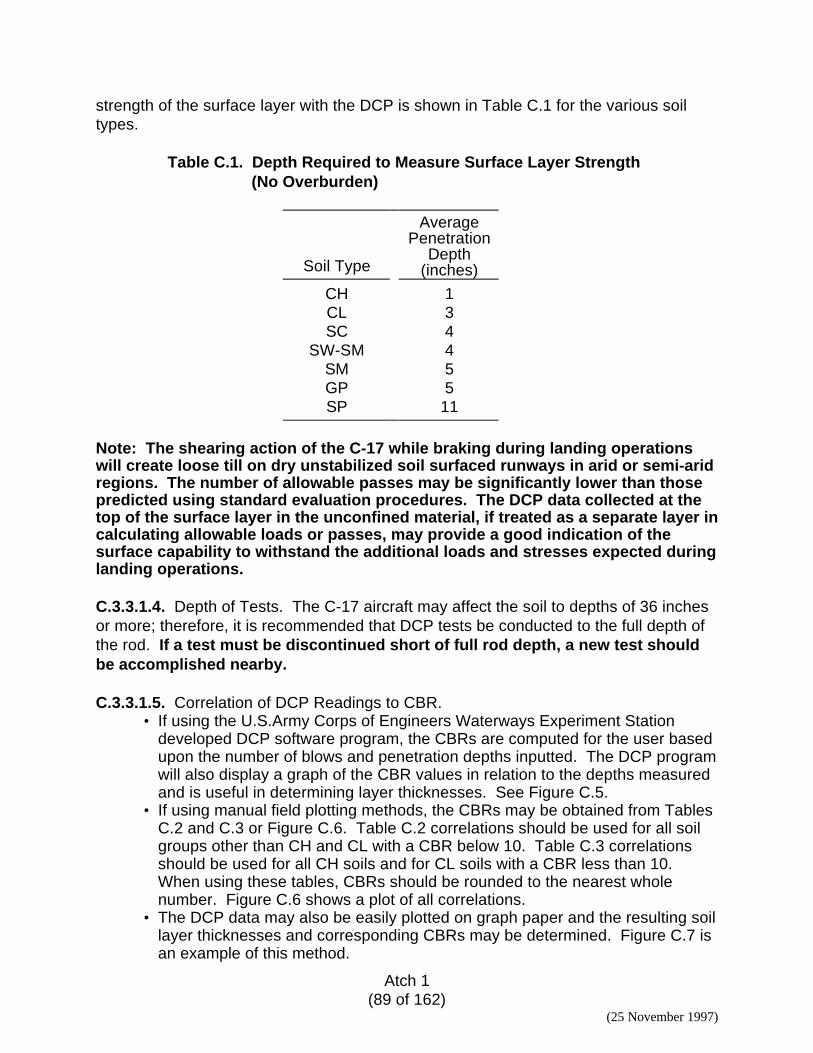
Atch 1(89 of 162)
(25 November 1997)
strength of the surface layer with the DCP is shown in Table C.1 for the various soiltypes.
Table C.1. Depth Required to Measure Surface Layer Strength(No Overburden)
Soil Type
AveragePenetration
Depth(inches)
CH 1CL 3SC 4
SW-SM 4SM 5GP 5SP 11
Note: The shearing action of the C-17 while braking during landing operationswill create loose till on dry unstabilized soil surfaced runways in arid or semi-aridregions. The number of allowable passes may be significantly lower than thosepredicted using standard evaluation procedures. The DCP data collected at thetop of the surface layer in the unconfined material, if treated as a separate layer incalculating allowable loads or passes, may provide a good indication of thesurface capability to withstand the additional loads and stresses expected duringlanding operations.
C.3.3.1.4. Depth of Tests. The C-17 aircraft may affect the soil to depths of 36 inchesor more; therefore, it is recommended that DCP tests be conducted to the full depth ofthe rod. If a test must be discontinued short of full rod depth, a new test shouldbe accomplished nearby.
C.3.3.1.5. Correlation of DCP Readings to CBR.• If using the U.S.Army Corps of Engineers Waterways Experiment Station
developed DCP software program, the CBRs are computed for the user basedupon the number of blows and penetration depths inputted. The DCP programwill also display a graph of the CBR values in relation to the depths measuredand is useful in determining layer thicknesses. See Figure C.5.
• If using manual field plotting methods, the CBRs may be obtained from TablesC.2 and C.3 or Figure C.6. Table C.2 correlations should be used for all soilgroups other than CH and CL with a CBR below 10. Table C.3 correlationsshould be used for all CH soils and for CL soils with a CBR less than 10.When using these tables, CBRs should be rounded to the nearest wholenumber. Figure C.6 shows a plot of all correlations.
• The DCP data may also be easily plotted on graph paper and the resulting soillayer thicknesses and corresponding CBRs may be determined. Figure C.7 isan example of this method.
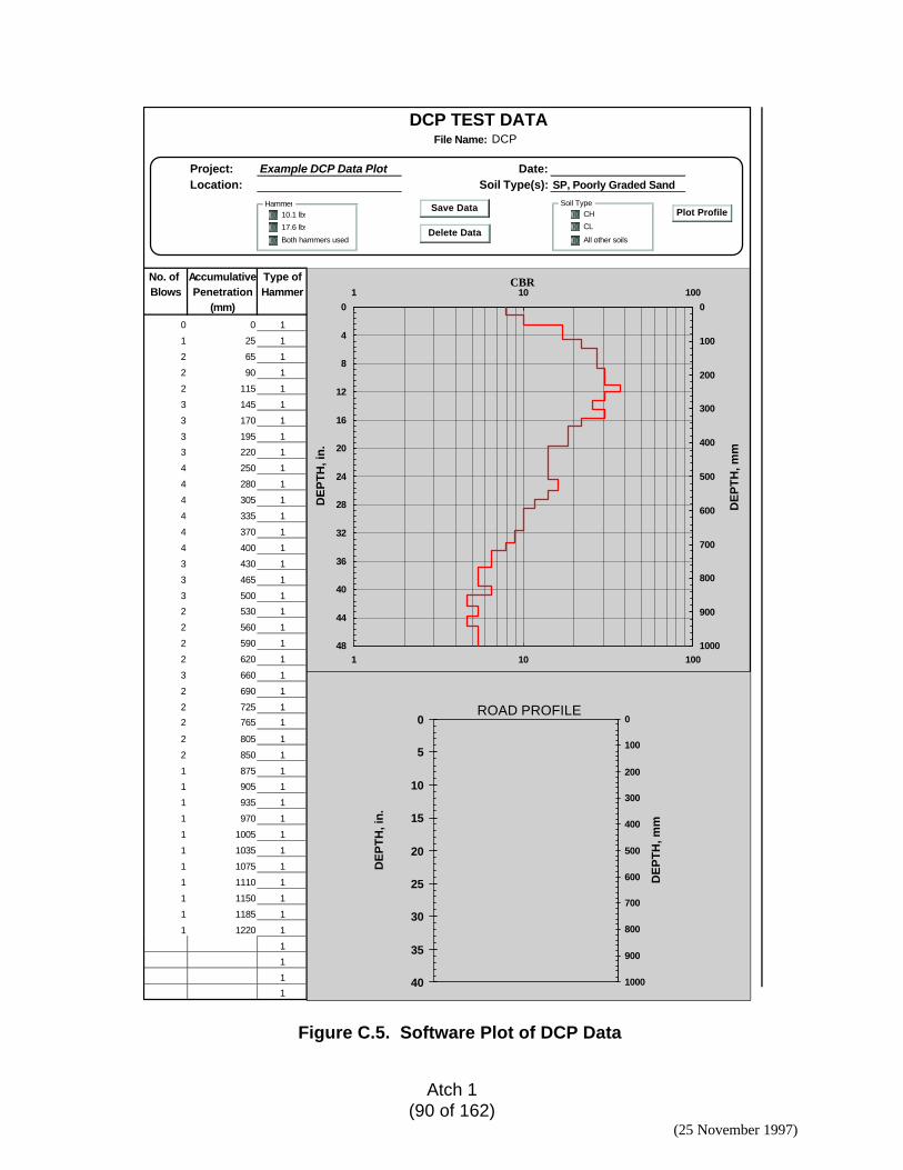
Atch 1(90 of 162)
(25 November 1997)
DCP TEST DATAFile Name: DCP
Project: Example DCP Data Plot Date:Location: Soil Type(s): SP, Poorly Graded Sand
4
No. of Accumulative Type ofBlows Penetration Hammer
(mm)
0 0 1
1 25 1
2 65 1
2 90 1
2 115 1
3 145 1
3 170 1
3 195 1
3 220 1
4 250 1
4 280 1
4 305 1
4 335 1
4 370 1
4 400 1
3 430 1
3 465 1
3 500 1
2 530 1
2 560 1
2 590 1
2 620 1
3 660 1
2 690 1
2 725 1
2 765 1
2 805 1
2 850 1
1 875 1
1 905 1
1 935 1
1 970 1
1 1005 1
1 1035 1
1 1075 1
1 1110 1
1 1150 1
1 1185 1
1 1220 1
1
1
1
1
Delete Data
0
4
8
12
16
20
24
28
32
36
40
44
48
1 10 100CBR
DE
PT
H, i
n.
0
100
200
300
400
500
600
700
800
900
10001 10 100
DE
PT
H, m
m
10.1 lbs
17.6 lbs
Both hammers used
Save Data Soil TypeCH
CL
All other soils
HammerPlot Profile
ROAD PROFILE0
5
10
15
20
25
30
35
40
DE
PT
H, i
n.
0
100
200
300
400
500
600
700
800
900
1000
DE
PT
H, m
m
ROAD PROFILE0
5
10
15
20
25
30
35
40
DE
PT
H, i
n.
0
100
200
300
400
500
600
700
800
900
1000
DE
PT
H, m
m
ROAD PROFILE0
5
10
15
20
25
30
35
40
DE
PT
H, i
n.
0
100
200
300
400
500
600
700
800
900
1000
DE
PT
H, m
m
ROAD PROFILE0
5
10
15
20
25
30
35
40
DE
PT
H, i
n.
0
100
200
300
400
500
600
700
800
900
1000
DE
PT
H, m
m
Figure C.5. Software Plot of DCP Data
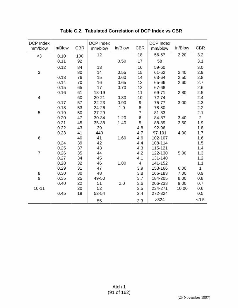
Atch 1(91 of 162)
(25 November 1997)
Table C.2. Tabulated Correlation of DCP Index vs CBR
DCP Indexmm/blow in/Blow CBR
DCP Indexmm/blow in/Blow CBR
DCP Indexmm/blow in/Blow CBR
<3 0.10 100 12 18 56-57 2.20 3.2
0.11 92 0.50 17 58 3.1
0.12 84 13 16 59-60 3.03 80 14 0.55 15 61-62 2.40 2.9
0.13 76 15 0.60 14 63-64 2.50 2.80.14 70 16 0.65 13 65-66 2.60 2.70.15 65 17 0.70 12 67-68 2.60.16 61 18-19 11 69-71 2.80 2.5
4 60 20-21 0.80 10 72-74 2.40.17 57 22-23 0.90 9 75-77 3.00 2.30.18 53 24-26 1.0 8 78-80 2.2
5 0.19 50 27-29 7 81-83 2.10.20 47 30-34 1.20 6 84-87 3.40 20.21 45 35-38 1.40 5 88-89 3.50 1.90.22 43 39 4.8 92-96 1.80.23 41 440 4.7 97-101 4.00 1.7
6 40 41 1.60 4.6 102-107 1.60.24 39 42 4.4 108-114 1.50.25 37 43 4.3 115-121 1.4
7 0.26 35 44 4.2 122-130 5.00 1.30.27 34 45 4.1 131-140 1.20.28 32 46 1.80 4 141-152 1.10.29 31 47 3.9 153-166 6.00 1
8 0.30 30 48 3.8 166-183 7.00 0.99 0.35 25 49-50 3.7 184-205 8.00 0.8
0.40 22 51 2.0 3.6 206-233 9.00 0.710-11 20 52 3.5 234-271 10.00 0.6
0.45 19 53-54 3.4 272-324 0.5
55 3.3 >324 <0.5
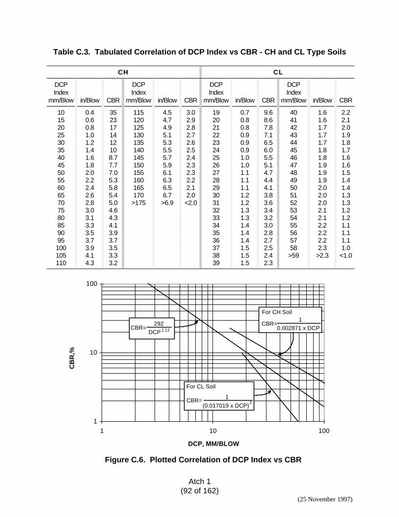
Atch 1(92 of 162)
(25 November 1997)
Table C.3. Tabulated Correlation of DCP Index vs CBR - CH and CL Type Soils
CH CL
DCPIndex
mm/Blow in/Blow CBR
DCPIndex
mm/Blow in/Blow CBR
DCPIndex
mm/Blow in/Blow CBR
DCPIndex
mm/Blow in/Blow CBR
10 0.4 35 115 4.5 3.0 19 0.7 9.6 40 1.6 2.215 0.6 23 120 4.7 2.9 20 0.8 8.6 41 1.6 2.120 0.8 17 125 4.9 2.8 21 0.8 7.8 42 1.7 2.025 1.0 14 130 5.1 2.7 22 0.9 7.1 43 1.7 1.930 1.2 12 135 5.3 2.6 23 0.9 6.5 44 1.7 1.835 1.4 10 140 5.5 2.5 24 0.9 6.0 45 1.8 1.740 1.6 8.7 145 5.7 2.4 25 1.0 5.5 46 1.8 1.645 1.8 7.7 150 5.9 2.3 26 1.0 5.1 47 1.9 1.650 2.0 7.0 155 6.1 2.3 27 1.1 4.7 48 1.9 1.555 2.2 5.3 160 6.3 2.2 28 1.1 4.4 49 1.9 1.460 2.4 5.8 165 6.5 2.1 29 1.1 4.1 50 2.0 1.465 2.6 5.4 170 6.7 2.0 30 1.2 3.8 51 2.0 1.370 2.8 5.0 >175 >6.9 <2.0 31 1.2 3.6 52 2.0 1.375 3.0 4.6 32 1.3 3.4 53 2.1 1.280 3.1 4.3 33 1.3 3.2 54 2.1 1.285 3.3 4.1 34 1.4 3.0 55 2.2 1.190 3.5 3.9 35 1.4 2.8 56 2.2 1.195 3.7 3.7 36 1.4 2.7 57 2.2 1.1100 3.9 3.5 37 1.5 2.5 58 2.3 1.0105 4.1 3.3 38 1.5 2.4 >59 >2.3 <1.0110 4.3 3.2 39 1.5 2.3
1
10
100
1 10 100
DCP, MM/BLOW
CB
R,%
(0.017019 x DCP)
For CL Soil
CBR= 1
2
For CH Soil
CBR=0.002871 x DCP
1CBR=
292
DCP 1.12
Figure C.6. Plotted Correlation of DCP Index vs CBR
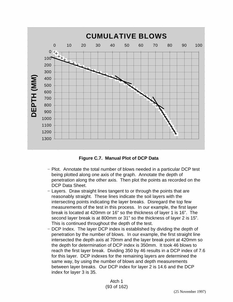
Atch 1(93 of 162)
(25 November 1997)
0
100
200
300
400
500
600
700
800
900
1000
1100
1200
1300
0 10 20 30 40 50 60 70 80 90 100
CUMULATIVE BLOWSD
EP
TH
(M
M)
Figure C.7. Manual Plot of DCP Data
− Plot. Annotate the total number of blows needed in a particular DCP testbeing plotted along one axis of the graph. Annotate the depth ofpenetration along the other axis. Then plot the points as recorded on theDCP Data Sheet.
− Layers. Draw straight lines tangent to or through the points that arereasonably straight. These lines indicate the soil layers with theintersecting points indicating the layer breaks. Disregard the top fewmeasurements of the test in this process. In our example, the first layerbreak is located at 420mm or 16” so the thickness of layer 1 is 16”. Thesecond layer break is at 800mm or 31” so the thickness of layer 2 is 15”.This is continued throughout the depth of the test.
− DCP Index. The layer DCP index is established by dividing the depth ofpenetration by the number of blows. In our example, the first straight lineintersected the depth axis at 70mm and the layer break point at 420mm sothe depth for determination of DCP index is 350mm. It took 46 blows toreach the first layer break. Dividing 350 by 46 results in a DCP index of 7.6for this layer. DCP indexes for the remaining layers are determined thesame way, by using the number of blows and depth measurementsbetween layer breaks. Our DCP index for layer 2 is 14.6 and the DCPindex for layer 3 is 35.
Atch 1(94 of 162)
(25 November 1997)
− CBRs. Tables C.2 and C.3 are then used to determine the CBRs for eachlayer. In our example, the soils tested were classified as SP or poorlygraded sand so we used Table C.2. Our depth measurements were inmilimeters so we enter the table in the DCP Index mm/blow columns asappropriate to find the corresponding CBRs. A CBR of 32 resulted for layer1, CBR 14 for layer 2, and CBR 5 for layer 3.
C.3.3.1.6. Special Considerations.• DCP tests in highly plastic clays are generally accurate for depths to
approximately 12 inches. At deeper depths, clay sticking to the lower rod mayindicate higher CBR values than actually exist. Oiling the rod will help, withoutsignificantly impacting the test results. It may be wise to auger out the testhole after each 12 inch depth encountered to eliminate the clay related frictionproblems and allow more accurate measurements.
• Many sands occur in a loose state. Such sands when relatively dry will showlow DCP index values for the top few inches and then may show increasingstrength with depth. The confining action of aircraft tires will increase thestrength of sand. All sands and gravels in a “quick” condition (waterpercolating through them) must be avoided. Evaluation of moist sands shouldbe based upon DCP test data.
• If the cone does not penetrate significantly (approximately one-half inch) after10 blows, the test should be stopped. If the material encountered is astabilized material or high strength aggregate base course which doesnot produce accurate results when penetrated with the DCP, it should becored or augered through its depth and the DCP operation resumedbeneath it. An appropriate CBR should be assigned to this layer. If largeaggregate is encountered, the test should be stopped and a new test shouldbe performed within a few feet of the first location. The DCP is generally notsuitable for soils having significant amounts of aggregate larger than 2inches. CBR values for unpenetrable materials must be carefully selectedbased upon their service behavior. Suggested CBR values for such materialsare:− Graded Crushed Aggregate 100− Macadam 100− Bituminous Binder 100− Limerock 80− Stabilized Aggregate 80− Soil Cement 80− Sand/Shell or Shell 80− Sand Asphalt 80
C.3.3.2. Other Strength Factors
C.3.3.2.1. Surface and Subsurface Drainage.• Locate depth of water table
Atch 1(95 of 162)
(25 November 1997)
• Look at contours in area, signs of surface drainage problems, and wet orswampy areas
• Coarse-grained soils have better internal drainage• Moisture content plays significant role in bearing capacity• Note the size and depth of any storm drain culverts under the pavement
C.3.3.2.2. Cut/fill areas indicate possible feature changes based on changingsubsurface layers.
C.3.3.2.3. Frost Areas.• Subgrade strengths are reduced significantly during thaw periods if the
potential exists for structural failure due to frost. Detrimental frost action willoccur if the subgrade contains frost-susceptible materials, the temperatureremains below freezing for a considerable amount of time, and an amplesupply of ground water is available. If all three conditions exist and frostdamage is apparent, Frost Area Soil Support Indexes (FASSIs) are used inlieu of CBRs.− F1 and S1 Soils = 9.0 FASSI− F2 and S2 Soils = 6.5 FASSI− F3 and F4 Soils = 3.5 FASSI
• Clays , silts, and some gravelly and sandy soils with high percentages of finesare frost susceptible. See Table C.4, Frost Design Soil Classifications.
• Areas of frost heave when no longer frozen may have large subsurface voidsand will not support projected loads. These areas must be properlyrecompacted.
C.3.3.2.4. Wet Climate.• Soil layer strengths in areas subject to heavy seasonal rains or flooding may
react similarly to those in frost susceptible areas. This is particularly true inthe case of fine-grained materials containing clays and/or silts where there isno adequate surface seal, or positive drainage away.
• Moisture conditions at the time of testing should be documented (Is it dry,damp, or wet?) and anticipated conditions for the projected usage period mustbe considered in determining the validity of test data for intended aircraftoperations.
C.4. Obtain Aircraft Operational Requirements
C.4.1. Obtain aircraft operational requirements from the Site Operations Officer, localCommand Section, or the tasking OPR.
C.4.2. Data Required for C-17 Aircraft
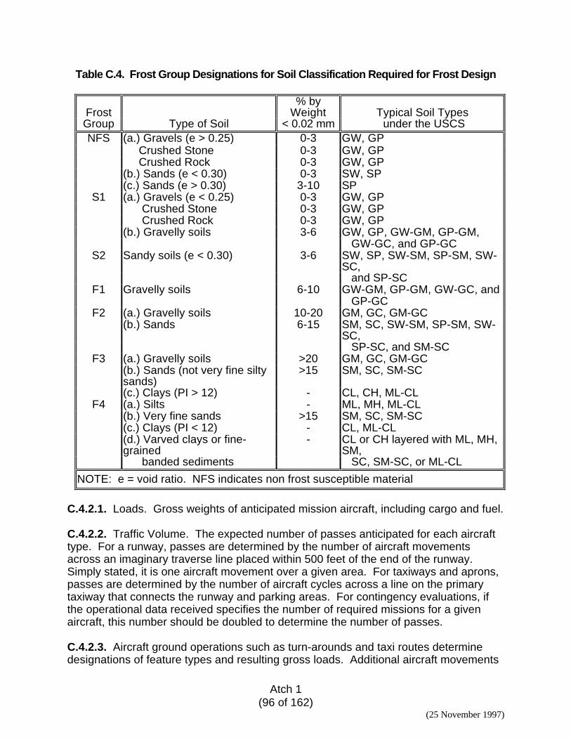
Atch 1(96 of 162)
(25 November 1997)
Table C.4. Frost Group Designations for Soil Classification Required for Frost Design
Frost% by
Weight Typical Soil TypesGroup Type of Soil < 0.02 mm under the USCSNFS (a.) Gravels (e > 0.25) 0-3 GW, GP
Crushed Stone 0-3 GW, GP Crushed Rock 0-3 GW, GP(b.) Sands (e < 0.30) 0-3 SW, SP(c.) Sands (e > 0.30) 3-10 SP
S1 (a.) Gravels (e < 0.25) 0-3 GW, GP Crushed Stone 0-3 GW, GP Crushed Rock 0-3 GW, GP(b.) Gravelly soils 3-6 GW, GP, GW-GM, GP-GM,
GW-GC, and GP-GCS2 Sandy soils (e < 0.30) 3-6 SW, SP, SW-SM, SP-SM, SW-
SC, and SP-SC
F1 Gravelly soils 6-10 GW-GM, GP-GM, GW-GC, and GP-GC
F2 (a.) Gravelly soils 10-20 GM, GC, GM-GC(b.) Sands 6-15 SM, SC, SW-SM, SP-SM, SW-
SC, SP-SC, and SM-SC
F3 (a.) Gravelly soils >20 GM, GC, GM-GC(b.) Sands (not very fine siltysands)
>15 SM, SC, SM-SC
(c.) Clays (PI > 12) - CL, CH, ML-CLF4 (a.) Silts - ML, MH, ML-CL
(b.) Very fine sands >15 SM, SC, SM-SC(c.) Clays (PI < 12) - CL, ML-CL(d.) Varved clays or fine-grained
- CL or CH layered with ML, MH,SM,
banded sediments SC, SM-SC, or ML-CL
NOTE: e = void ratio. NFS indicates non frost susceptible material
C.4.2.1. Loads. Gross weights of anticipated mission aircraft, including cargo and fuel.
C.4.2.2. Traffic Volume. The expected number of passes anticipated for each aircrafttype. For a runway, passes are determined by the number of aircraft movementsacross an imaginary traverse line placed within 500 feet of the end of the runway.Simply stated, it is one aircraft movement over a given area. For taxiways and aprons,passes are determined by the number of aircraft cycles across a line on the primarytaxiway that connects the runway and parking areas. For contingency evaluations, ifthe operational data received specifies the number of required missions for a givenaircraft, this number should be doubled to determine the number of passes.
C.4.2.3. Aircraft ground operations such as turn-arounds and taxi routes determinedesignations of feature types and resulting gross loads. Additional aircraft movements
Atch 1(97 of 162)
(25 November 1997)
on the runway, i.e. back-taxiing in the case of an airfield with no parallel taxiway andapron system, will also increase the number of passes per each planned mission.
C.5. Conduct Surface Condition Visual Assessment. Visual surveys of the airfieldsurface can provide information on apparent structural integrity, operational condition,and projected performance. A cursory inspection of the features should be performedand the distress types, quantities, and severity levels as described in Appendix Bshould be identified. The features should then be assigned overall condition ratings.
C.6. Refine Airfield Layout/Compile Summary of Physical Property Data (PPD).Update the airfield layout based upon aircraft operational requirements, surfacecondition assessment, and results of field test data. Each feature should now bedistinguishable by the characteristics of surface type, thickness, and condition;subsurface layer types, thicknesses, and strengths; construction history; use; and traffictype. One method to consolidate the cross section or pavement system profile dataobtained from field tests and construction history into specific features is to:
C.6.1. Arrange pavement and soil profile data in relation to the actual test locations onthe airfield. This will show the range of values and relationship of any given testlocation data to that at adjacent test locations.
C.6.2. Group those containing common characteristics into features.
C.6.3. Establish the representative profile for each feature. In most cases, the CBRvalues selected for a feature should be a low average of those collected from all thetest locations within the feature, but this is not always true. Conditions are seldomuniform and sound engineering judgment should be used.
C.6.4. Compile the characteristics for each feature into the Summary of PPD. Thisinformation will be used to determine the allowable gross loads and/or allowablepasses for the airfield (see Figure C.8).
C.7. Determine Allowable Gross Loads (AGLs)/ Allowable Passes
C.7.1. Semi-Prepared Airfields. Semi-prepared airfields may be evaluated for variousaircraft using the US Army Waterways Experiment Station developed software programUNSEVA, Computer Aided Evaluation of Expedient Airfields or manually using FigureC.9, CBR Nomograph and Semi-Prepared Surface Evaluation Curve, Figure C.10.
C.7.1.1. If using the UNSEVA program:
C.7.1.1.1. Double-click on the icon to bring up the Expedient Airfields screen. Inputsfrom this screen are somewhat self-explanatory.
C.7.1.1.2. Choose the aircraft type from the list.
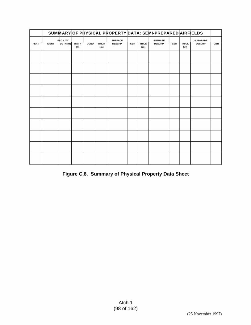
Atch 1(98 of 162)
(25 November 1997)
SUMMARY OF PHYSICAL PROPERTY DATA: SEMI-PREPARED AIRFIELDS
FACILITY SURFACE SUBBASE SUBGRADEFEAT IDENT LGTH (ft) WDTH
(ft)COND THICK
(in)DESCRP CBR THICK
(in)DESCRP CBR THICK
(in)DESCRP CBR
Figure C.8. Summary of Physical Property Data Sheet
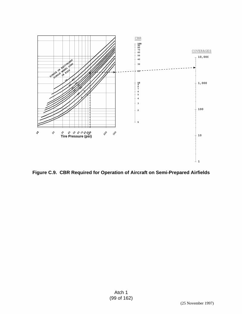
Atch 1(99 of 162)
(25 November 1997)
10 20 30 40 50 60 70 80 90100
200
30010 100
Tire Pressure (psi)
75 60
5040
35
30
2520
10
52
1
SINGLE OR EQUIVALENT
SINGLE WHEEL LOAD
IN KIPS
1
2
3
4
5
678910
20
30
40
50
60708090100
1
10
100
1
10
100
1,000
10,000
CBR
COVERAGES
Figure C.9. CBR Required for Operation of Aircraft on Semi-Prepared Airfields
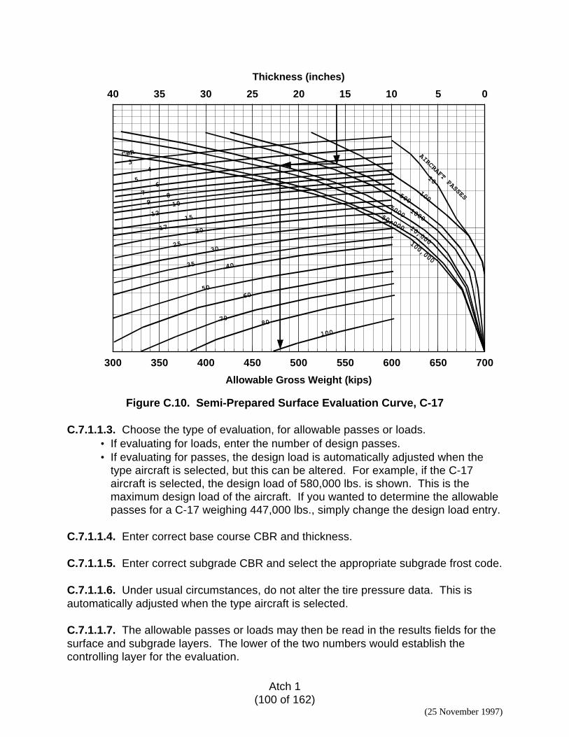
Atch 1(100 of 162)
(25 November 1997)
300 350 400 450 500 550 600 650 700
Allowable Gross Weight (kips)
0510152025303540
Thickness (inches)
AIRCRAFT PASSES100
10,000
50,000
5000 1000
100,000
500
CBR
34
56
7 89 10
1215
17 20
2530
35 40
5060
7080
100
10
Figure C.10. Semi-Prepared Surface Evaluation Curve, C-17
C.7.1.1.3. Choose the type of evaluation, for allowable passes or loads.• If evaluating for loads, enter the number of design passes.• If evaluating for passes, the design load is automatically adjusted when the
type aircraft is selected, but this can be altered. For example, if the C-17aircraft is selected, the design load of 580,000 lbs. is shown. This is themaximum design load of the aircraft. If you wanted to determine the allowablepasses for a C-17 weighing 447,000 lbs., simply change the design load entry.
C.7.1.1.4. Enter correct base course CBR and thickness.
C.7.1.1.5. Enter correct subgrade CBR and select the appropriate subgrade frost code.
C.7.1.1.6. Under usual circumstances, do not alter the tire pressure data. This isautomatically adjusted when the type aircraft is selected.
C.7.1.1.7. The allowable passes or loads may then be read in the results fields for thesurface and subgrade layers. The lower of the two numbers would establish thecontrolling layer for the evaluation.
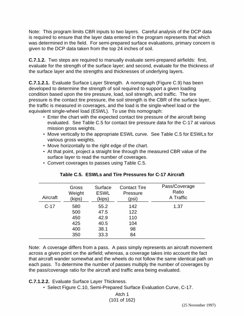
Atch 1(101 of 162)
(25 November 1997)
Note: This program limits CBR inputs to two layers. Careful analysis of the DCP datais required to ensure that the layer data entered in the program represents that whichwas determined in the field. For semi-prepared surface evaluations, primary concern isgiven to the DCP data taken from the top 24 inches of soil.
C.7.1.2. Two steps are required to manually evaluate semi-prepared airfields: first,evaluate for the strength of the surface layer; and second, evaluate for the thickness ofthe surface layer and the strengths and thicknesses of underlying layers.
C.7.1.2.1. Evaluate Surface Layer Strength. A nomograph (Figure C.9) has beendeveloped to determine the strength of soil required to support a given loadingcondition based upon the tire pressure, load, soil strength, and traffic. The tirepressure is the contact tire pressure, the soil strength is the CBR of the surface layer,the traffic is measured in coverages, and the load is the single-wheel load or theequivalent single-wheel load (ESWL). To use this nomograph:
• Enter the chart with the expected contact tire pressure of the aircraft beingevaluated. See Table C.5 for contact tire pressure data for the C-17 at variousmission gross weights.
• Move vertically to the appropriate ESWL curve. See Table C.5 for ESWLs forvarious gross weights.
• Move horizontally to the right edge of the chart.• At that point, project a straight line through the measured CBR value of the
surface layer to read the number of coverages.• Convert coverages to passes using Table C.5.
Table C.5. ESWLs and Tire Pressures for C-17 Aircraft
Aircraft
GrossWeight(kips)
SurfaceESWL(kips)
Contact TirePressure
(psi)
Pass/CoverageRatio
A Traffic
C-17 580 55.2 142 1.37500 47.5 122450 42.9 110425 40.5 104400 38.1 98350 33.3 84
Note: A coverage differs from a pass. A pass simply represents an aircraft movementacross a given point on the airfield; whereas, a coverage takes into account the factthat aircraft wander somewhat and the wheels do not follow the same identical path oneach pass. To determine the number of passes multiply the number of coverages bythe pass/coverage ratio for the aircraft and traffic area being evaluated.
C.7.1.2.2. Evaluate Surface Layer Thickness.• Select Figure C.10, Semi-Prepared Surface Evaluation Curve, C-17.
Atch 1(102 of 162)
(25 November 1997)
• Using the layer data from the PPD, enter the top of the chart with the thicknessof the aggregate surface layer. Draw a vertical line (Line 1) downward throughthe aircraft pass levels. Also enter the bottom of the chart at the desired grossweight, draw a line vertically to the curve depicting the CBR of the layerimmediately beneath the surface layer, then horizontally to intersect Line 1.This point of intersection defines the allowable number of passes. If thisnumber is equal to or exceeds the number of passes computed during theevaluation of the surface layer strength then the thickness of the surface layeris adequate.
Note: This step evaluates the layer immediately beneath the surface layer as well asthe thickness of the surface layer.
C.7.1.2.3. Evaluate remaining subsurface layers. Repeat this procedure for each soillayer. Enter the top of the chart with the thickness above the layer being evaluated anduse the CBR of the layer being evaluated. The layer that produces the lowestallowable number of passes is the controlling layer for the evaluation.
Example: Determine the allowable number of passes for a 400,000 lb. C-17 aircraft onthe following soil cross section in an A traffic area:
8” Aggregate Surface Course, CBR: 208” Subbase Course, CBR: 15Subgrade, CBR: 5
Solution:• Step 1, Evaluate Surface Course Strength:
− Enter the nomograph chart at 98 PSI, the expected contact tire pressure forthe C-17.
− Move vertically to the 38.1 ESWL curve and then horizontally to the rightedge of the chart.
− Draw a straight line from this point through the CBR line at 20 and read4,000 coverages.
− Multiply 4,000 coverages by 1.37 to determine the allowable number ofpasses, which is 5,480.
• Step 2, Evaluate Surface Layer Thickness:− Select the Semi-Prepared Surface Evaluation Curve for the C-17.− Enter the top of the chart at 8 inches drawing a vertical line (Line 1)
downward through the aircraft pass curves.− Enter the bottom of the chart at 400,000 lbs and draw a vertical line up to
the 15 CBR curve, then horizontally to intersect with Line 1.− The point of intersection indicates an allowable pass number of
approximately 2,500.• Step 3, Evaluate the Subgrade:
− Enter the top of the chart at 16 inches drawing a vertical line (Line 1)downward through the aircraft passes.
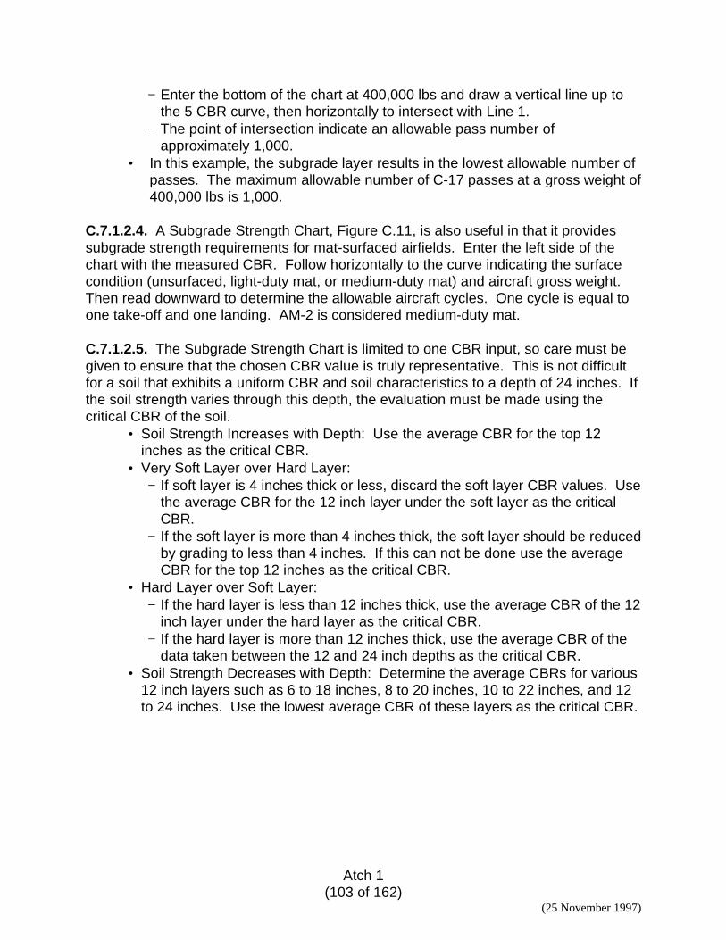
Atch 1(103 of 162)
(25 November 1997)
− Enter the bottom of the chart at 400,000 lbs and draw a vertical line up tothe 5 CBR curve, then horizontally to intersect with Line 1.
− The point of intersection indicate an allowable pass number ofapproximately 1,000.
• In this example, the subgrade layer results in the lowest allowable number ofpasses. The maximum allowable number of C-17 passes at a gross weight of400,000 lbs is 1,000.
C.7.1.2.4. A Subgrade Strength Chart, Figure C.11, is also useful in that it providessubgrade strength requirements for mat-surfaced airfields. Enter the left side of thechart with the measured CBR. Follow horizontally to the curve indicating the surfacecondition (unsurfaced, light-duty mat, or medium-duty mat) and aircraft gross weight.Then read downward to determine the allowable aircraft cycles. One cycle is equal toone take-off and one landing. AM-2 is considered medium-duty mat.
C.7.1.2.5. The Subgrade Strength Chart is limited to one CBR input, so care must begiven to ensure that the chosen CBR value is truly representative. This is not difficultfor a soil that exhibits a uniform CBR and soil characteristics to a depth of 24 inches. Ifthe soil strength varies through this depth, the evaluation must be made using thecritical CBR of the soil.
• Soil Strength Increases with Depth: Use the average CBR for the top 12inches as the critical CBR.
• Very Soft Layer over Hard Layer:− If soft layer is 4 inches thick or less, discard the soft layer CBR values. Use
the average CBR for the 12 inch layer under the soft layer as the criticalCBR.
− If the soft layer is more than 4 inches thick, the soft layer should be reducedby grading to less than 4 inches. If this can not be done use the averageCBR for the top 12 inches as the critical CBR.
• Hard Layer over Soft Layer:− If the hard layer is less than 12 inches thick, use the average CBR of the 12
inch layer under the hard layer as the critical CBR.− If the hard layer is more than 12 inches thick, use the average CBR of the
data taken between the 12 and 24 inch depths as the critical CBR.• Soil Strength Decreases with Depth: Determine the average CBRs for various
12 inch layers such as 6 to 18 inches, 8 to 20 inches, 10 to 22 inches, and 12to 24 inches. Use the lowest average CBR of these layers as the critical CBR.
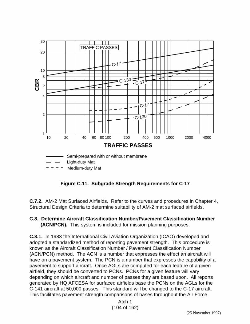
Atch 1(104 of 162)
(25 November 1997)
10 20 40 1008060 200 400 1000 40002000600
30
20
10
8
6
4
2
1
CB
R
TRAFFIC PASSES
Semi-prepared with or without membraneLight-duty MatMedium-duty Mat
TRAFFIC PASSES
C-17
C-17
C-17
C-130
C-130
Figure C.11. Subgrade Strength Requirements for C-17
C.7.2. AM-2 Mat Surfaced Airfields. Refer to the curves and procedures in Chapter 4,Structural Design Criteria to determine suitability of AM-2 mat surfaced airfields.
C.8. Determine Aircraft Classification Number/Pavement Classification Number(ACN/PCN). This system is included for mission planning purposes.
C.8.1. In 1983 the International Civil Aviation Organization (ICAO) developed andadopted a standardized method of reporting pavement strength. This procedure isknown as the Aircraft Classification Number / Pavement Classification Number(ACN/PCN) method. The ACN is a number that expresses the effect an aircraft willhave on a pavement system. The PCN is a number that expresses the capability of apavement to support aircraft. Once AGLs are computed for each feature of a givenairfield, they should be converted to PCNs. PCNs for a given feature will varydepending on which aircraft and number of passes they are based upon. All reportsgenerated by HQ AFCESA for surfaced airfields base the PCNs on the AGLs for theC-141 aircraft at 50,000 passes. This standard will be changed to the C-17 aircraft.This facilitates pavement strength comparisons of bases throughout the Air Force.
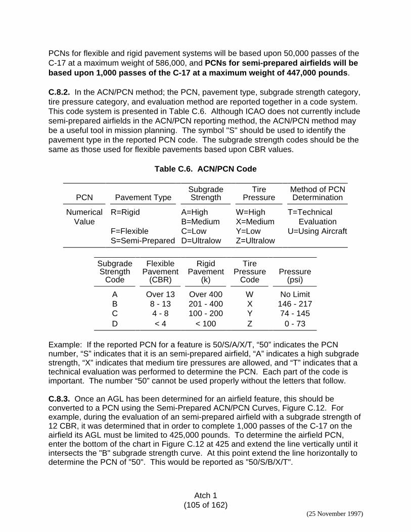
Atch 1(105 of 162)
(25 November 1997)
PCNs for flexible and rigid pavement systems will be based upon 50,000 passes of theC-17 at a maximum weight of 586,000, and PCNs for semi-prepared airfields will bebased upon 1,000 passes of the C-17 at a maximum weight of 447,000 pounds.
C.8.2. In the ACN/PCN method; the PCN, pavement type, subgrade strength category,tire pressure category, and evaluation method are reported together in a code system.This code system is presented in Table C.6. Although ICAO does not currently includesemi-prepared airfields in the ACN/PCN reporting method, the ACN/PCN method maybe a useful tool in mission planning. The symbol "S" should be used to identify thepavement type in the reported PCN code. The subgrade strength codes should be thesame as those used for flexible pavements based upon CBR values.
Table C.6. ACN/PCN Code
PCN Pavement TypeSubgradeStrength
TirePressure
Method of PCNDetermination
NumericalValue
R=Rigid A=HighB=Medium
W=HighX=Medium
T=TechnicalEvaluation
F=Flexible C=Low Y=Low U=Using AircraftS=Semi-Prepared D=Ultralow Z=Ultralow
SubgradeStrength
Code
FlexiblePavement
(CBR)
RigidPavement
(k)
TirePressure
CodePressure
(psi)
A Over 13 Over 400 W No LimitB 8 - 13 201 - 400 X 146 - 217C 4 - 8 100 - 200 Y 74 - 145D < 4 < 100 Z 0 - 73
Example: If the reported PCN for a feature is 50/S/A/X/T, “50” indicates the PCNnumber, “S” indicates that it is an semi-prepared airfield, “A” indicates a high subgradestrength, “X” indicates that medium tire pressures are allowed, and “T” indicates that atechnical evaluation was performed to determine the PCN. Each part of the code isimportant. The number “50” cannot be used properly without the letters that follow.
C.8.3. Once an AGL has been determined for an airfield feature, this should beconverted to a PCN using the Semi-Prepared ACN/PCN Curves, Figure C.12. Forexample, during the evaluation of an semi-prepared airfield with a subgrade strength of12 CBR, it was determined that in order to complete 1,000 passes of the C-17 on theairfield its AGL must be limited to 425,000 pounds. To determine the airfield PCN,enter the bottom of the chart in Figure C.12 at 425 and extend the line vertically until itintersects the "B" subgrade strength curve. At this point extend the line horizontally todetermine the PCN of "50". This would be reported as "50/S/B/X/T".
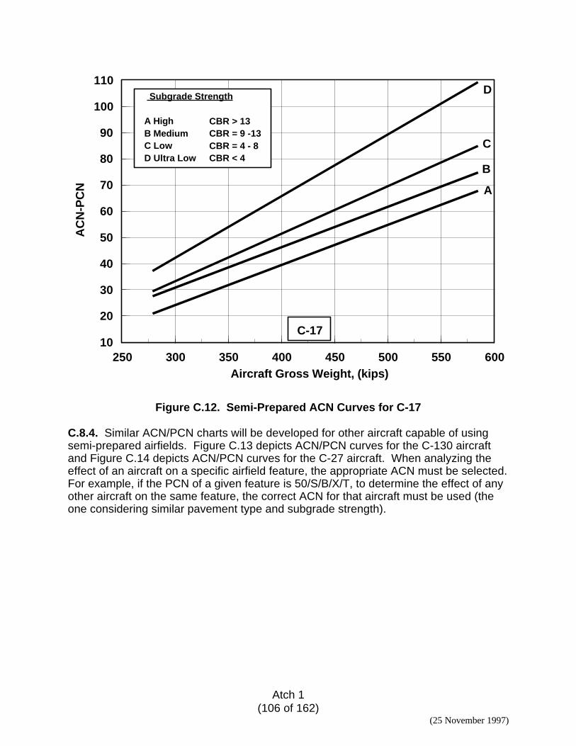
Atch 1(106 of 162)
(25 November 1997)
250 300 350 400 450 500 550 600Aircraft Gross Weight, (kips)
10
20
30
40
50
60
70
80
90
100
110A
CN
-PC
N A
C-17
B
C
D Subgrade Strength
A High B Medium C Low D Ultra Low
CBR > 13CBR = 9 -13 CBR = 4 - 8 CBR < 4
Figure C.12. Semi-Prepared ACN Curves for C-17
C.8.4. Similar ACN/PCN charts will be developed for other aircraft capable of usingsemi-prepared airfields. Figure C.13 depicts ACN/PCN curves for the C-130 aircraftand Figure C.14 depicts ACN/PCN curves for the C-27 aircraft. When analyzing theeffect of an aircraft on a specific airfield feature, the appropriate ACN must be selected.For example, if the PCN of a given feature is 50/S/B/X/T, to determine the effect of anyother aircraft on the same feature, the correct ACN for that aircraft must be used (theone considering similar pavement type and subgrade strength).
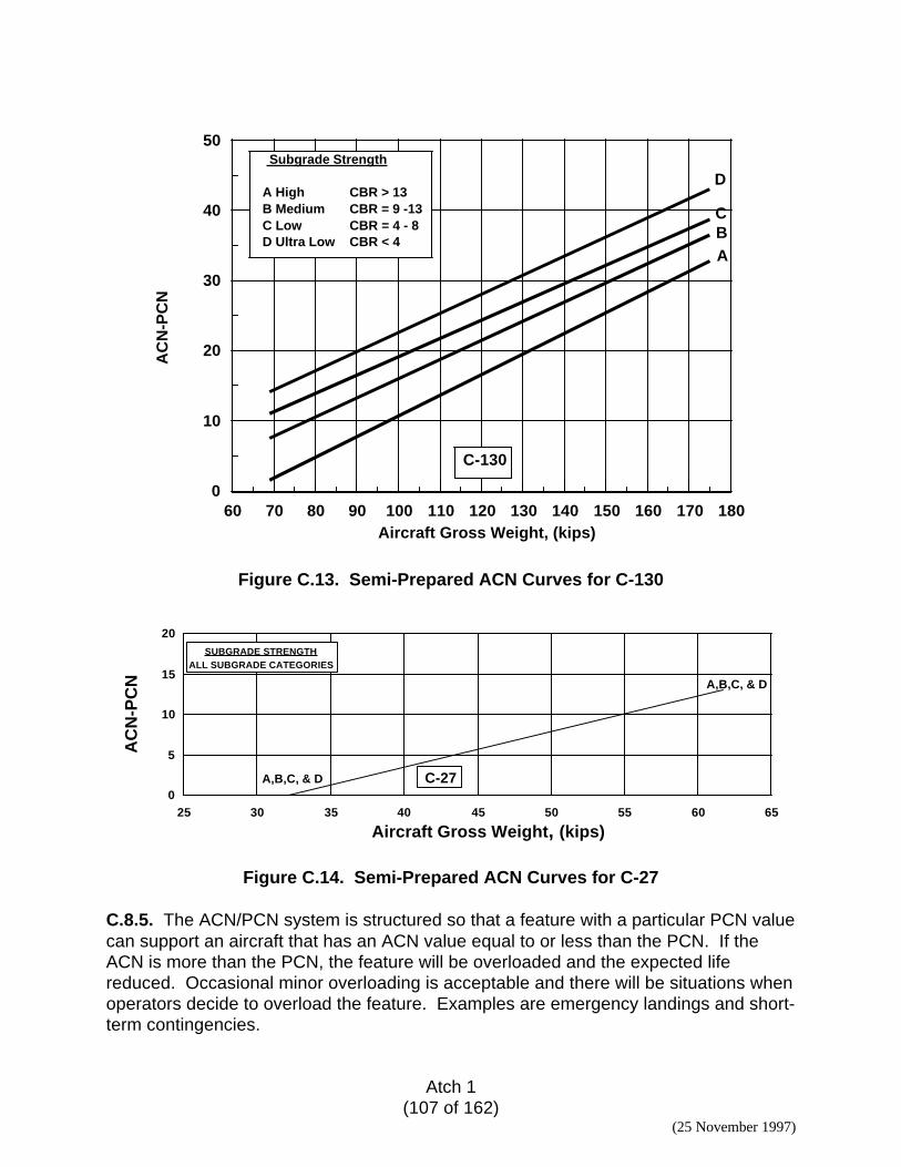
Atch 1(107 of 162)
(25 November 1997)
60 70 80 90 100 110 120 130 140 150 160 170 180Aircraft Gross Weight, (kips)
0
10
20
30
40
50A
CN
-PC
N
ABC
D Subgrade Strength
A High B Medium C Low D Ultra Low
CBR > 13CBR = 9 -13 CBR = 4 - 8 CBR < 4
C-130
Figure C.13. Semi-Prepared ACN Curves for C-130
C-270
5
10
15
20
25 30 35 40 45 50 55 60 65
Aircraft Gross Weight, (kips)
AC
N-P
CN
SUBGRADE STRENGTHALL SUBGRADE CATEGORIES
A,B,C, & D
A,B,C, & D
Figure C.14. Semi-Prepared ACN Curves for C-27
C.8.5. The ACN/PCN system is structured so that a feature with a particular PCN valuecan support an aircraft that has an ACN value equal to or less than the PCN. If theACN is more than the PCN, the feature will be overloaded and the expected lifereduced. Occasional minor overloading is acceptable and there will be situations whenoperators decide to overload the feature. Examples are emergency landings and short-term contingencies.

Atch 1(108 of 162)
(25 November 1997)
• Overload movements should not be allowed on pavements exhibiting signs ofstructural distresses or failure.
• For frost susceptible regions, overloading should be avoided during periods ofthaw or when the subgrade appears weakened.
• For seasonally wet regions, overloading should be avoided if the subgradeappears saturated or weakened by water.
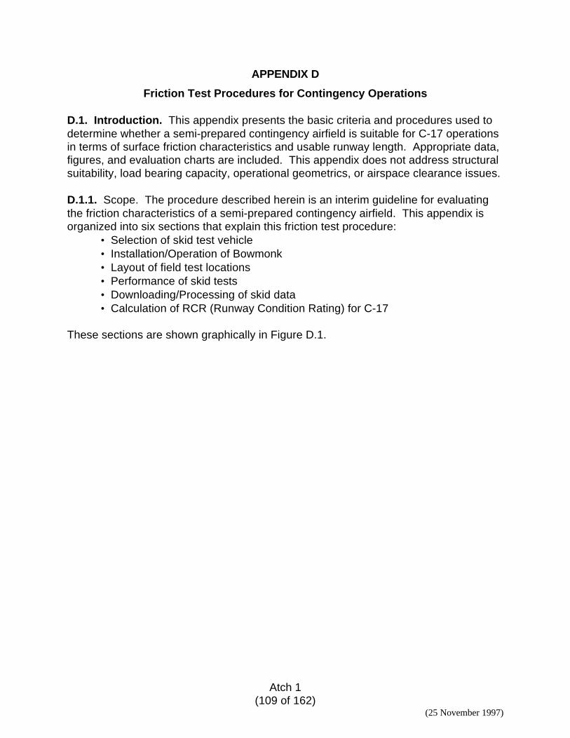
Atch 1(109 of 162)
(25 November 1997)
APPENDIX D
Friction Test Procedures for Contingency Operations
D.1. Introduction. This appendix presents the basic criteria and procedures used todetermine whether a semi-prepared contingency airfield is suitable for C-17 operationsin terms of surface friction characteristics and usable runway length. Appropriate data,figures, and evaluation charts are included. This appendix does not address structuralsuitability, load bearing capacity, operational geometrics, or airspace clearance issues.
D.1.1. Scope. The procedure described herein is an interim guideline for evaluatingthe friction characteristics of a semi-prepared contingency airfield. This appendix isorganized into six sections that explain this friction test procedure:
• Selection of skid test vehicle• Installation/Operation of Bowmonk• Layout of field test locations• Performance of skid tests• Downloading/Processing of skid data• Calculation of RCR (Runway Condition Rating) for C-17
These sections are shown graphically in Figure D.1.
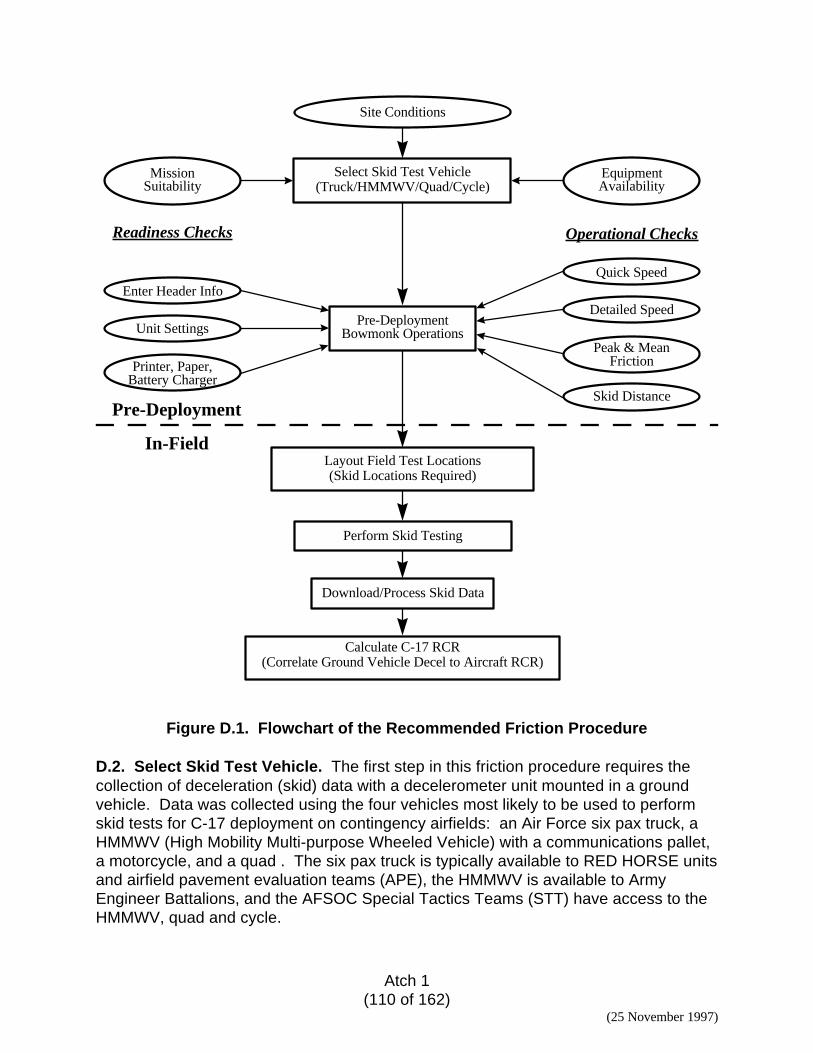
Atch 1(110 of 162)
(25 November 1997)
Pre-DeploymentBowmonk Operations
Select Skid Test Vehicle(Truck/HMMWV/Quad/Cycle)
MissionSuitability
Site Conditions
Perform Skid Testing
Download/Process Skid Data
Layout Field Test Locations(Skid Locations Required)
Calculate C-17 RCR(Correlate Ground Vehicle Decel to Aircraft RCR)
EquipmentAvailability
Readiness Checks
Enter Header Info
Unit Settings
Printer, Paper,Battery Charger
Operational Checks
Quick Speed
Detailed Speed
Peak & MeanFriction
Skid DistancePre-Deployment
In-Field
Figure D.1. Flowchart of the Recommended Friction Procedure
D.2. Select Skid Test Vehicle. The first step in this friction procedure requires thecollection of deceleration (skid) data with a decelerometer unit mounted in a groundvehicle. Data was collected using the four vehicles most likely to be used to performskid tests for C-17 deployment on contingency airfields: an Air Force six pax truck, aHMMWV (High Mobility Multi-purpose Wheeled Vehicle) with a communications pallet,a motorcycle, and a quad . The six pax truck is typically available to RED HORSE unitsand airfield pavement evaluation teams (APE), the HMMWV is available to ArmyEngineer Battalions, and the AFSOC Special Tactics Teams (STT) have access to theHMMWV, quad and cycle.
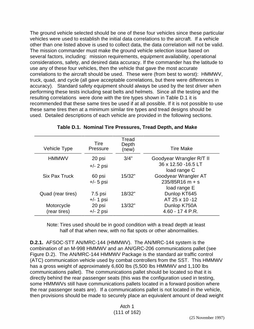
Atch 1(111 of 162)
(25 November 1997)
The ground vehicle selected should be one of these four vehicles since these particularvehicles were used to establish the initial data correlations to the aircraft. If a vehicleother than one listed above is used to collect data, the data correlation will not be valid.The mission commander must make the ground vehicle selection issue based onseveral factors, including: mission requirements, equipment availability, operationalconsiderations, safety, and desired data accuracy. If the commander has the latitude touse any of these four vehicles, then the vehicle that gave the most accuratecorrelations to the aircraft should be used. These were (from best to worst): HMMWV,truck, quad, and cycle (all gave acceptable correlations, but there were differences inaccuracy). Standard safety equipment should always be used by the test driver whenperforming these tests including seat belts and helmets. Since all the testing and theresulting correlations were done with the tire types shown in Table D.1 it isrecommended that these same tires be used if at all possible. If it is not possible to usethese same tires then at a minimum similar tire types and tread designs should beused. Detailed descriptions of each vehicle are provided in the following sections.
Table D.1. Nominal Tire Pressures, Tread Depth, and Make
Vehicle TypeTire
Pressure
TreadDepth(new) Tire Make
HMMWV 20 psi
+/- 2 psi
3/4” Goodyear Wrangler R/T II36 x 12.50 -16.5 LT
load range CSix Pax Truck 60 psi
+/- 5 psi15/32” Goodyear Wrangler AT
235/85R16 m + sload range E
Quad (rear tires) 7.5 psi+/- 1 psi
18/32” Dunlop KT645AT 25 x 10 -12
Motorcycle(rear tires)
20 psi+/- 2 psi
13/32” Dunlop K750A4.60 - 17 4 P.R.
Note: Tires used should be in good condition with a tread depth at leasthalf of that when new, with no flat spots or other abnormalities.
D.2.1. AFSOC-STT AN/MRC-144 (HMMWV). The AN/MRC-144 system is thecombination of an M-998 HMMWV and an AN/GRC-206 communications pallet (seeFigure D.2). The AN/MRC-144 HMMWV Package is the standard air traffic control(ATC) communication vehicle used by combat controllers from the SST. This HMMWVhas a gross weight of approximately 6,600 lbs (5,500 lbs HMMWV and 1,100 lbscommunications pallet). The communications pallet should be located so that it isdirectly behind the rear passenger seats (this was the configuration used in testing,some HMMWVs still have communications pallets located in a forward position wherethe rear passenger seats are). If a communications pallet is not located in the vehicle,then provisions should be made to securely place an equivalent amount of dead weight
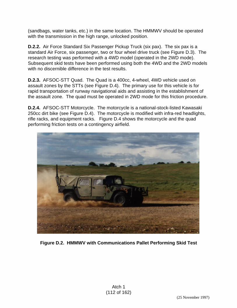
Atch 1(112 of 162)
(25 November 1997)
(sandbags, water tanks, etc.) in the same location. The HMMWV should be operatedwith the transmission in the high range, unlocked position.
D.2.2. Air Force Standard Six Passenger Pickup Truck (six pax). The six pax is astandard Air Force, six passenger, two or four wheel drive truck (see Figure D.3). Theresearch testing was performed with a 4WD model (operated in the 2WD mode).Subsequent skid tests have been performed using both the 4WD and the 2WD modelswith no discernible difference in the test results.
D.2.3. AFSOC-STT Quad. The Quad is a 400cc, 4-wheel, 4WD vehicle used onassault zones by the STTs (see Figure D.4). The primary use for this vehicle is forrapid transportation of runway navigational aids and assisting in the establishment ofthe assault zone. The quad must be operated in 2WD mode for this friction procedure.
D.2.4. AFSOC-STT Motorcycle. The motorcycle is a national-stock-listed Kawasaki250cc dirt bike (see Figure D.4). The motorcycle is modified with infra-red headlights,rifle racks, and equipment racks. Figure D.4 shows the motorcycle and the quadperforming friction tests on a contingency airfield.
Figure D.2. HMMWV with Communications Pallet Performing Skid Test
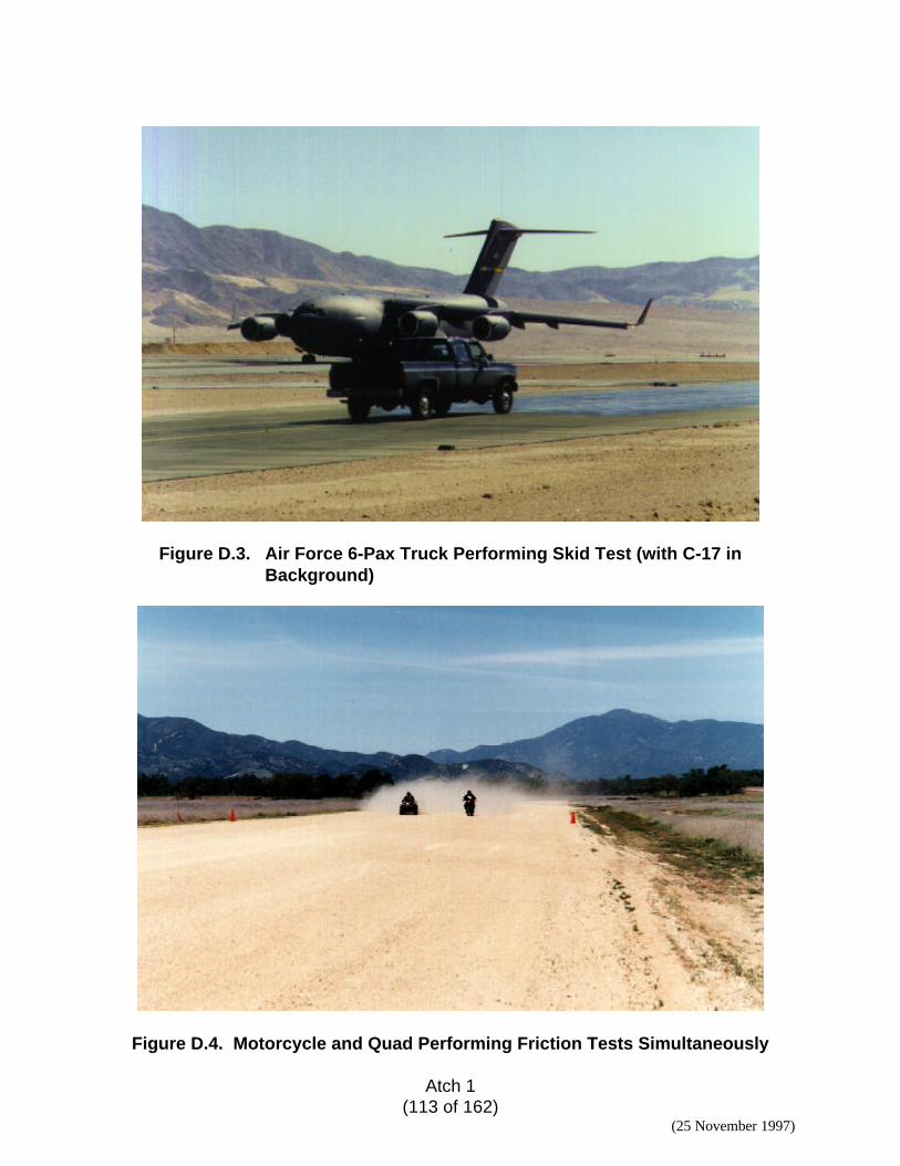
Atch 1(113 of 162)
(25 November 1997)
Figure D.3. Air Force 6-Pax Truck Performing Skid Test (with C-17 inBackground)
Figure D.4. Motorcycle and Quad Performing Friction Tests Simultaneously
Atch 1(114 of 162)
(25 November 1997)
D.3. Bowmonk Unit. The Bowmonk Airfield Friction Meter Mk II was the device usedfor this research testing. The use of any other device is not recommended since thedata correlations were developed with this unit. The Bowmonk is manufactured inEngland and was designed to provide airfield managers with a simple, consistent, andautomated method for predicting the available friction between the aircraft tires andrunway surface. The unit was originally designed for use on paved runway surfaces,such as asphalt or concrete, but has now been evaluated for applicability to skid testingon semi-prepared contingency airfields. A skid test is performed with the decelerometerunit installed on a flat and level surface in the ground vehicle and the resulting groundvehicle deceleration measurement is used to predict aircraft stopping performance. Inthis section, the hardware will be discussed, the fundamental measurements will bedescribed, specific installation recommendations will be provided, and procedures fortesting and operating the Bowmonk will be detailed.
D.3.1. Hardware Description. The Bowmonk unit measures approximately 6 inches by9 inches by 3 inches, and weighs only 6 pounds. It is relatively simple to operate andis portable for field use. The unit is battery powered and can operate for up to 16hours in the field on a single charge. If necessary it may be recharged or operated witha 12 VDC cigarette lighter plug found in most vehicles. The Bowmonk includes aconnection for exporting data via an RS-232 serial port to a personal computer forpermanent storage and analysis.
The internal memory of the Bowmonk AFM-2 will hold up to 99 tests before it must bedownloaded to a PC. A stripchart printer is provided for real-time hardcopy printouts ofthe data in the field. See Figure D.5 for a close up of the instrument panel of theBowmonk unit.
D.3.2. Measurement Parameters. The Bowmonk measures the deceleration of thevehicle during a skid test. The values are reported as a percentage of the accelerationdue to gravity (%g). Both peak and average (mean) calculated decelerations areprovided, as well as calculated stopping distance, time of deceleration, and velocity atthe start of the skid. This ground vehicle deceleration data can then be correlated tothe required aircraft Runway Condition Rating (RCR) for comparing available runwaylength to stopping distance required by the aircraft.
D.3.3. Bowmonk Installation. In the HMMWV and six pax the Bowmonk unit is placedbeside the driver and secured in a horizontal configuration. With the motorcycle andquad, the unit is placed on the equipment racks. The unit should be horizontal to within15 degrees. The unit does not have to be perfectly level, since it has an internalsoftware routine that compensates for small deviations from level. It will be necessaryto construct plywood boxes to use the units with the six pax, quad, and cycle. The boxfor the six pax should be constructed so that it will hold the Bowmonk unit securely andallow the unit to be strapped in level on the front seat using the middle seat belt. Boxesfor the quad and cycle should be constructed so that they hold the units firmly (so theunits can be slid in and out of the boxes), and these boxes should be attached to theequipment racks with plastic wire/zip ties. Bungee cord should be placed across the
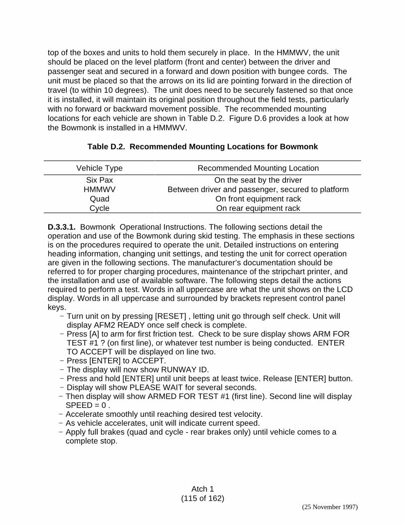
Atch 1(115 of 162)
(25 November 1997)
top of the boxes and units to hold them securely in place. In the HMMWV, the unitshould be placed on the level platform (front and center) between the driver andpassenger seat and secured in a forward and down position with bungee cords. Theunit must be placed so that the arrows on its lid are pointing forward in the direction oftravel (to within 10 degrees). The unit does need to be securely fastened so that onceit is installed, it will maintain its original position throughout the field tests, particularlywith no forward or backward movement possible. The recommended mountinglocations for each vehicle are shown in Table D.2. Figure D.6 provides a look at howthe Bowmonk is installed in a HMMWV.
Table D.2. Recommended Mounting Locations for Bowmonk
Vehicle Type Recommended Mounting Location
Six Pax On the seat by the driverHMMWV Between driver and passenger, secured to platform
Quad On front equipment rackCycle On rear equipment rack
D.3.3.1. Bowmonk Operational Instructions. The following sections detail theoperation and use of the Bowmonk during skid testing. The emphasis in these sectionsis on the procedures required to operate the unit. Detailed instructions on enteringheading information, changing unit settings, and testing the unit for correct operationare given in the following sections. The manufacturer’s documentation should bereferred to for proper charging procedures, maintenance of the stripchart printer, andthe installation and use of available software. The following steps detail the actionsrequired to perform a test. Words in all uppercase are what the unit shows on the LCDdisplay. Words in all uppercase and surrounded by brackets represent control panelkeys.
− Turn unit on by pressing [RESET] , letting unit go through self check. Unit willdisplay AFM2 READY once self check is complete.
− Press [A] to arm for first friction test. Check to be sure display shows ARM FORTEST #1 ? (on first line), or whatever test number is being conducted. ENTERTO ACCEPT will be displayed on line two.
− Press [ENTER] to ACCEPT.− The display will now show RUNWAY ID.− Press and hold [ENTER] until unit beeps at least twice. Release [ENTER] button.− Display will show PLEASE WAIT for several seconds.− Then display will show ARMED FOR TEST #1 (first line). Second line will display
SPEED = 0 .− Accelerate smoothly until reaching desired test velocity.− As vehicle accelerates, unit will indicate current speed.− Apply full brakes (quad and cycle - rear brakes only) until vehicle comes to a
complete stop.
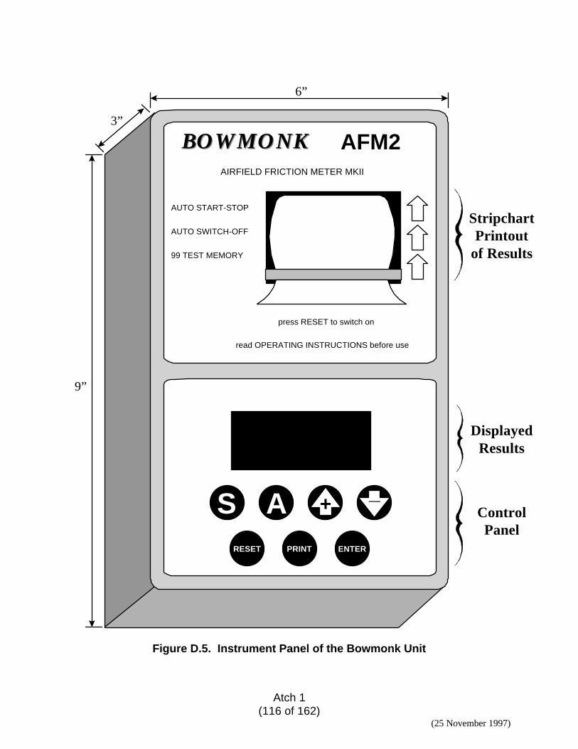
Atch 1(116 of 162)
(25 November 1997)
A + _
BOWMONKBOWMONKAIRFIELD FRICTION METER MKII
AFM2
AUTO START-STOP
AUTO SWITCH-OFF
99 TEST MEMORY
press RESET to switch on
read OPERATING INSTRUCTIONS before use
RESET PRINT ENTER
S
6”
3”
9”
StripchartPrintout
of Results
DisplayedResults
ControlPanel
Figure D.5. Instrument Panel of the Bowmonk Unit
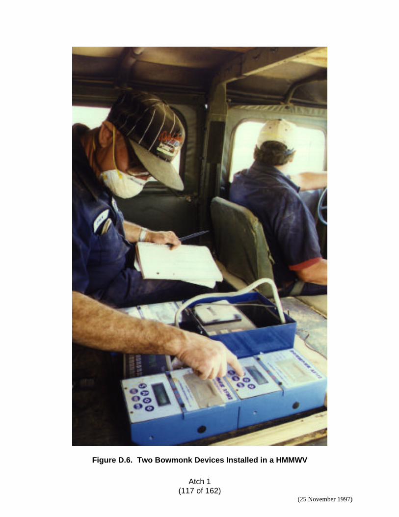
Atch 1(117 of 162)
(25 November 1997)
Figure D.6. Two Bowmonk Devices Installed in a HMMWV
Atch 1(118 of 162)
(25 November 1997)
− Unit will display DON’T MOVE - CALCULATING.− Keep the vehicle stationary to allow unit to complete its internal calculations and
display results.− Unit will now display measured PERCENT G (first line) and SPEED (second line).− If the results are acceptable, save the test results by pressing [A] to accept this
test. The unit will now display AFM2 READY.− If the result is not acceptable, press [RESET], the instrument will discard the
current test and display AFM2 READY. Another test can be performed and savedwith the same test number.
− Ready vehicle for next test and repeat from step 2 to perform subsequent tests.
Continue until desired number of friction tests are completed. The Bowmonk unit willautomatically shut down after 4 minutes of inactivity to save the battery. To turn it backon, simply press [RESET], testing can then continue . To check the amount of memoryused and the battery condition press and hold [RESET] once unit is on and displayingAFM2 READY. Release [RESET] to return to normal on state. This is recommended iflarge numbers of tests are conducted or battery is suspected to be low. Print out and/ordownload data if memory approaches full or battery level becomes low to avoid a lossof data.
D.3.3.2. Printing Test Results. After completion of the friction tests, the followingsteps are required to print out a summary of the test results. A results summary printoutfrom a series of tests is shown in Figure D.7. Note that the friction values are the peakfriction measurements (not mean). Also note that the overall average is an average ofthe peak friction measurements. The overall average peak friction value (63%g inFigure D.7) can be used in Table D.7 to calculate a C-17 RCR. However, an overallaverage mean friction value is highly preferable to a peak value for determining anRCR. The results are more consistent and the measurement is less likely to be madeincorrectly.
− After completion/acceptance of last test, display will show AFM2 READY− If unit has shutdown press [RESET] to turn unit back on.− Press [PRINT] . The display will show PRINT TEST FOR RUNWAY ?− (check the instrument and make sure it shows correct RUNWAY ID).− Data may have inadvertently been collected under more than one runway id.− The [UP ARROW] and [DOWN ARROW] can be used to select runway id to print.− Press ENTER once (this will print a results summary stripchart report that shows
the test number, the calculated velocity at braking, and the peak friction results forall tests performed.
− Remove stripchart printout, label with additional information if necessary (vehicle,driver, test conditions) and store in an appropriate place.
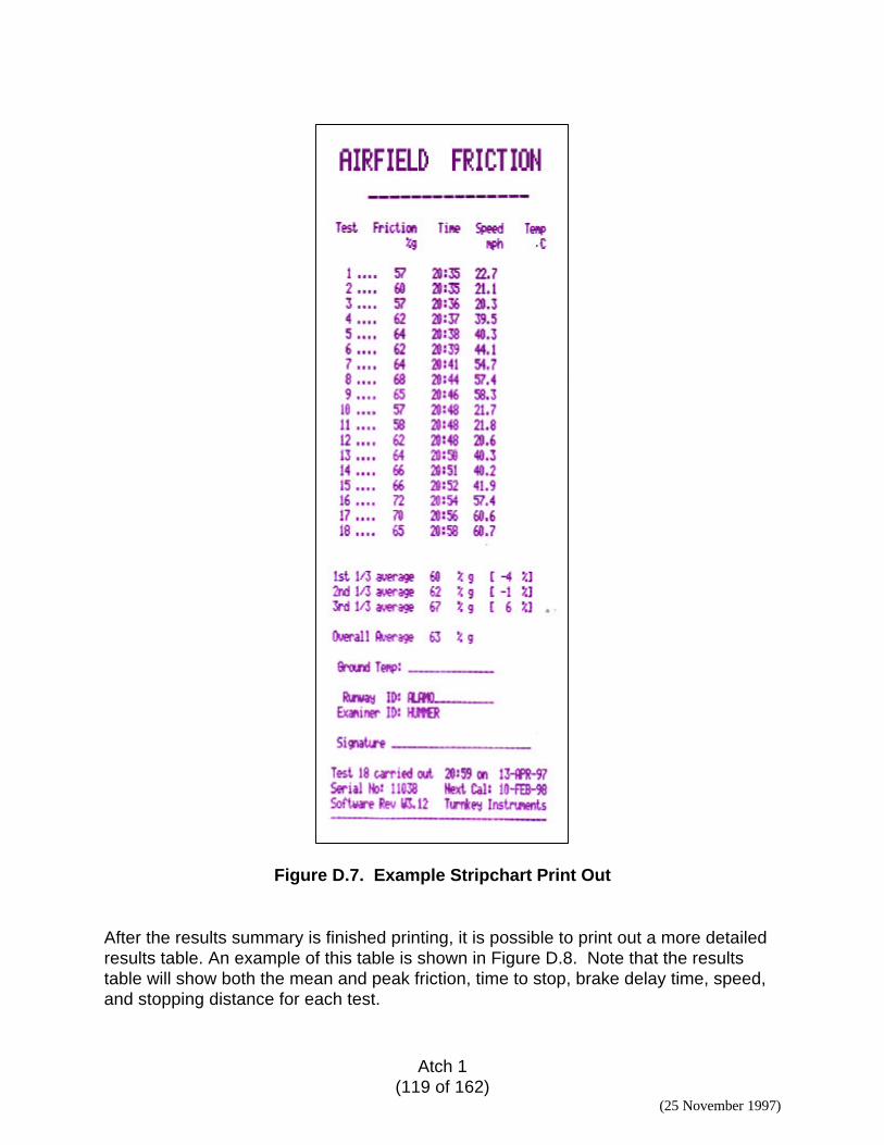
Atch 1(119 of 162)
(25 November 1997)
Figure D.7. Example Stripchart Print Out
After the results summary is finished printing, it is possible to print out a more detailedresults table. An example of this table is shown in Figure D.8. Note that the resultstable will show both the mean and peak friction, time to stop, brake delay time, speed,and stopping distance for each test.
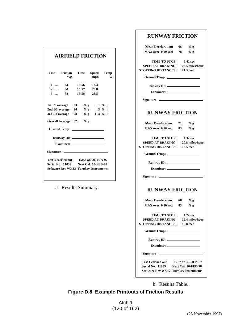
Atch 1(120 of 162)
(25 November 1997)
AIRFIELD FRICTION
Test Friction%g
Time Speedmph
TempC
123
838478
….….….
15:5615:5715:58
18.420.823.5
1st 1/3 average2nd 1/3 average3rd 1/3 average
838478 % g
% g% g
[ -4 % ][ 3 % ][ 1 % ]
Overall Average 82 % g
Ground Temp:
Runway ID:
Examiner:
Signature
Test 3 carried out 15:58 on 26-JUN-97Serial No: 11039 Next Cal: 10-FEB-98Software Rev W3.12 Turnkey Instruments
RUNWAY FRICTION
Mean Deceleration: 66 % g
MAX over 0.20 sec: 78 % g
TIME TO STOP: 1.41 secSPEED AT BRAKING: 23.5 miles/hour
STOPPING DISTANCES: 21.3 feet
Ground Temp:
Runway ID:
Examiner:
Signature
RUNWAY FRICTION
Mean Deceleration: 71 % g
MAX over 0.20 sec: 83 % g
TIME TO STOP: 1.32 secSPEED AT BRAKING: 20.8 miles/hour
STOPPING DISTANCES: 19.5 feet
Ground Temp:
Runway ID:
Examiner:
Signature
RUNWAY FRICTION
Mean Deceleration: 68 % g
MAX over 0.20 sec: 83 % g
TIME TO STOP: 1.22 secSPEED AT BRAKING: 18.4 miles/hour
STOPPING DISTANCES: 15.8 feet
Ground Temp:
Runway ID:
Examiner:
Signature
Test 1 carried out 15:57 on 26-JUN-97Serial No: 11039 Next Cal: 10-FEB-98Software Rev W3.12 Turnkey Instruments
a. Results Summary.
b. Results Table.
Figure D.8 Example Printouts of Friction Results
Atch 1(121 of 162)
(25 November 1997)
To print out a results table, continue with the following steps:− Press [PRINT] for a second time.− Use [UP ARROW] or [DOWN ARROW] to select test number to print.− Press [ENTER] to start printing a results table for that test number.
All the tests stored in the unit can also be printed. The following steps can be used toprint the results tables from the test number indicated on the unit up to the last testcarried out.
− Unit will display PRINT TEST N.− Press [A] instead of [ENTER] as described in the steps above. This only applies to
a results table printout.− Unit will print results tables from test N up to the last test carried out.− Press [RESET] at anytime to terminate printout.
See Figure D.8-b (Results Table) printout for an example. Note that both peak andmean values are given for each test. If using the mean friction value measurements todetermine a C-17 RCR, then the average for all the means must be calculated. Afterperforming the skid tests in the number and manner described elsewhere in thisappendix, a results table must be printed out for each test. Total the mean values foreach test then divide that total by the number of tests to determine the overall averagemean friction value for that series of tests. As an example, look at the data shown inFigure D.8-b (Results Table). The three mean friction values are 66%g, 71%g, and68%g. The total value is 205%g. Divide 205%g by a total of three tests for an averagemean value of 68.3%g for this series of tests. This overall average mean friction valueis the number that is used in Table D.7 to calculate a C-17 RCR. An overall averagemean friction value is highly preferable to an overall average peak friction value fordetermining a C-17 RCR.
D.3.3.3. Download Skid Data. The following procedure is to be used for uploadingdata from the Bowmonk Mk II Airfield Friction Meter to a field laptop or portablecomputer. This procedure is not critical to contingency airfield operations, but it doespreserve the data collected in more detail and allow for a more in-depth analysis of thedata later if necessary. Field computer must meet these minimum requirements : 386SXprocessor, at least 4 MB of RAM, a hard disk with at least 4 MB of free space, oneRS232 serial port, VGA or SVGA screen, a mouse, and Microsoft Windows 3.1 or later.The manufacturer supplied program (AFM2 for Windows) must also be installed on thefield computer. Note that only the software and Bowmonk units purchased together arecompatible due to the encoding of serial numbers on the units and software. Units andsoftware purchased separately will not work.
− Attach manufacturer supplied download cable to both Bowmonk and RS232 serialport of computer.
− Press [RESET] on Bowmonk to turn on if not already on.− Press and hold [RESET].
Atch 1(122 of 162)
(25 November 1997)
− Unit will display battery voltage and percent memory used. If percent memory usedis greater than 95%, then unit should not be downloaded (doing so will causesoftware to crash and will corrupt computer database, resulting in loss of data andrequiring re-installation of software).
− If data in Bowmonk has not been printed, it should be done now (in case ofdownloading problems).
− If memory used was > 95%, then unit must be cleared and tests redone.− Start up “AFM2 for Windows” program in Windows on the laptop computer.− Note the serial numbers that are displayed when program starts up. Check to see
if the unit you wish to download matches one of these numbers The serial numberof the unit is located on the bottom of the test summary strip chart printout. If notthen data cannot be downloaded.
− Click on OK button on windows program to start it.− Click on UPLOAD button to begin process of uploading.− During the upload do not disturb the computer, Bowmonk , or connecting cable.− Once uploading is complete, access and browse through database to ensure that
the recently collected test data has downloaded.− Exit database. If another unit is not going to be downloaded immediately, then exit
completely from the AFM2 program. If the AFM2 program remains running and thecomputer suffers from a glitch, lockup, or shutdown due to sleep mode or lowbattery, the database will be corrupted, resulting in loss of data and requiring re-installation of software.
− Disconnect cable and shutdown both the Bowmonk and computer to save power ifthey are not going to be used immediately.
− Reset unit to prepare for next series of tests.
D.3.3.4. Clearing and Resetting Bowmonk. The following steps are required to readythe unit for the next series of tests. This procedure will clear out all the test resultscollected so far. Unit settings will not be affected by this procedure.
− Press [RESET] to turn unit on if not already on.− Display will show AFM2 READY.− Press [ENTER] to enter Editing Mode.− Use [UP ARROW] and [DOWN ARROW] to move between menus.− Move to CLEAR MY MEMORY? menu.− Press [ENTER].− Unit will display ALL RECORDS LOST?, PRESS [ENTER] TO ACCEPT, [RESET]
TO ESCAPE.− Press [ENTER] to clear memory.− Unit will display AFM2 READY.− Press [S] and [PRINT] at the same time to turn unit off.
D.3.4. Predeployment Operational Checks and Procedures. The following sectionsdetail procedures that can be performed as predeployment steps to save time in thefield or verify proper functioning of unit before actual deployment.
Atch 1(123 of 162)
(25 November 1997)
D.3.4.1. Entering Header Information. This section details the steps necessary toenter "Header" information in the Bowmonk unit. This can be done before arriving onsite to save time in the field. The unit will retain this information until it is changed.Entering this information is useful for data documentation but not necessary for properoperation of the unit.
− Press [RESET] to turn unit on if not already on. Unit will display AFM2 READY.− Press [ENTER]. The display will show EDITING MODE.− Press [UP ARROW] and the display will show EXAMINER ID.− Press [ENTER] again. You may now enter the Examiner ID.− Use the [UP ARROW] and [DOWN ARROW] to select a letter.− Press [ENTER] to accept that letter and move to the next letter.− Press and hold [ENTER] when Examiner ID is correctly input.− The display will now show RUNWAY ID.− Press [ENTER] again to enter the Runway ID.− Use the [UP ARROW] and [DOWN ARROW] to select a letter.− Press [ENTER] to accept that letter and move on to the next letter.− Press and hold [ENTER] when Runway ID is correctly input.− The display will show NAME OF AIRPORT.− Press [ENTER] again to enter the Name of Airport− Use [UP ARROW] and [DOWN ARROW] to select a letter.− Press [ENTER] to accept that letter and move on to the next letter.− Press and hold [ENTER] when Name of Airport is correct.− Press the [RESET] . The display will now read AFM2 READY.
D.3.4.2.1. Bowmonk Configuration Menus. The following sections detail the stepsnecessary to access and modify important unit settings. These settings should not bemodified unless they differ from settings recommended in this appendix. It should notbe necessary to perform any of these modifications. This section is included mainly todocument these settings and provide a way for the user to check them should the unitnot appear to be operating correctly. Each Bowmonk unit comes with a manufacturersupplied password. This is to prevent inadvertent changes to important unit settingswhich is possible (without a password) due to the nature of the control panel. It is highlyrecommended that the password for the unit be documented and stored in multiplelocations and accessible in the field. Some settings cannot be modified or evenchecked without the password. Anyone using the password to check or modify settingsshould use caution and document any setting numbers before and after any changes.The manufacture’s user manual should also be consulted. If the correct password isgiven to the Configuration Prompt in the Editing Mode, the following menus appear:
a) Advanced Setupb) Trim Parametersc) Trim Zerosd) Adjust Clocke) Re-Calibrate
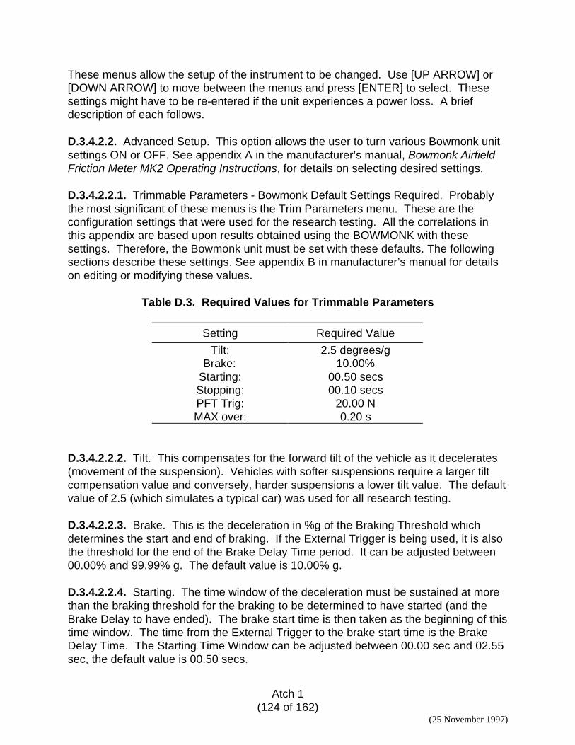
Atch 1(124 of 162)
(25 November 1997)
These menus allow the setup of the instrument to be changed. Use [UP ARROW] or[DOWN ARROW] to move between the menus and press [ENTER] to select. Thesesettings might have to be re-entered if the unit experiences a power loss. A briefdescription of each follows.
D.3.4.2.2. Advanced Setup. This option allows the user to turn various Bowmonk unitsettings ON or OFF. See appendix A in the manufacturer’s manual, Bowmonk AirfieldFriction Meter MK2 Operating Instructions, for details on selecting desired settings.
D.3.4.2.2.1. Trimmable Parameters - Bowmonk Default Settings Required. Probablythe most significant of these menus is the Trim Parameters menu. These are theconfiguration settings that were used for the research testing. All the correlations inthis appendix are based upon results obtained using the BOWMONK with thesesettings. Therefore, the Bowmonk unit must be set with these defaults. The followingsections describe these settings. See appendix B in manufacturer’s manual for detailson editing or modifying these values.
Table D.3. Required Values for Trimmable Parameters
Setting Required Value
Tilt: 2.5 degrees/gBrake: 10.00%
Starting: 00.50 secsStopping: 00.10 secsPFT Trig: 20.00 NMAX over: 0.20 s
D.3.4.2.2.2. Tilt. This compensates for the forward tilt of the vehicle as it decelerates(movement of the suspension). Vehicles with softer suspensions require a larger tiltcompensation value and conversely, harder suspensions a lower tilt value. The defaultvalue of 2.5 (which simulates a typical car) was used for all research testing.
D.3.4.2.2.3. Brake. This is the deceleration in %g of the Braking Threshold whichdetermines the start and end of braking. If the External Trigger is being used, it is alsothe threshold for the end of the Brake Delay Time period. It can be adjusted between00.00% and 99.99% g. The default value is 10.00% g.
D.3.4.2.2.4. Starting. The time window of the deceleration must be sustained at morethan the braking threshold for the braking to be determined to have started (and theBrake Delay to have ended). The brake start time is then taken as the beginning of thistime window. The time from the External Trigger to the brake start time is the BrakeDelay Time. The Starting Time Window can be adjusted between 00.00 sec and 02.55sec, the default value is 00.50 secs.
Atch 1(125 of 162)
(25 November 1997)
D.3.4.2.2.5. Stopping. The time window (after a valid start) of the deceleration must besustained at less than braking threshold for the braking to be determined to haveended (and the vehicle to have stopped). The brake end time is then taken as thebeginning of this time window. The time between the brake start and brake end timesis the Braking Time. The average deceleration will be calculated over this intervalunless you have specifically included in the average the deceleration during the BrakeDelay Time as well. The Stopping Time Window can be adjusted between 00.00 secand 02.55 sec, the default value is 00.10 secs.
D.3.4.2.2.6. PFT Trig. This is the brake pedal force in Newtons required to trigger theinstrument when using the pedal force transducer. Not applicable to the BowmonkAFM2 model unit.
D.3.4.2.2.7. Max Over. The time window interval in seconds over which the developedor sustained peak friction reading is determined. This setting will cause the frictionvalue to be the greatest lowest value seen as the window is scanned across the data.
D.3.4.2.3. Trim Parameters. The Bowmonk unit is programmed with some adjustableparameters whose values can be changed. This editing option allows their value to bechanged.
D.3.4.2.4. Trim Zeros. This menu allows the user to periodically check and trim thetransducer zero levels. Zeroing can be done on any flat surface by following theprompts on the display. Properly trimmed zeros allow the instrument to be used tomake accurate measurements of ground slope. Note that the zero trimming surfacedoes not have to be exactly horizontal but it must be flat. Make the first measurementwith the instrument handle nearest to you, then rotate the instrument through 180degrees and make the second measurement with the handle pointed away from you.
D.3.4.2.5. Adjust Clock. This menu allows the time to be changed to compensate fordaylight savings time. On selection, the minutes value will flash to indicate it can beadjusted, press [UP ARROW] or [DOWN ARROW] to change, then [ENTER] to savethe new value. The hours value will then flash and can be adjusted likewise. The datecan only be changed at the factory.
D.3.4.2.6. Re-Calibrate. Shows the latest calibration information and allows thefactory/distributor to re-calibrate the instrument. Press [P] to print a calibration report.Calibration reports are supplied by the manufacturer when a unit is purchased or re-calibrated. Copies of this report should be made and stored in appropriate locations forfuture reference. Units must be shipped back to manufacturer once a year for yearlycalibration.
D.3.5. Operational Checks. The following sections detail procedures that can beperformed before or after deployment if necessary to verify proper operation of theBowmonk unit. These are recommended as predeployment activities due to the lengthof time and manpower required to perform these tests. These tests are also useful for
Atch 1(126 of 162)
(25 November 1997)
operators who need to become familiar with the operation and accuracy of these units.In the process of performing these procedures, all safety considerations and vehicleskidding procedures described in this appendix should still be followed.
D.3.5.1. Quick Verification of Speed Measurement. For this operational check, a long,flat, level area is required. The Bowmonk unit is placed in the vehicle of choice asrecommended. The unit is armed and operated as normal. Make sure the unit displaysa speed of 0.0 when starting and that the vehicle is accelerated smoothly anduniformly. As the vehicle increases in speed towards the target speed, the driverwatches the speed as displayed on the Bowmonk (this is impossible on the cycle, andin the HMMWV and six pax a passenger to observe the unit is helpful). If whenreaching target speed the difference between the speedometer and the Bowmonk isless than 5% then the unit is likely working correctly. Multiple units can also be usedsimultaneously to make comparisons between Bowmonk units. This test assumes thatthe vehicle speedometer is accurate and functioning correctly.
D.3.5.2. Detailed Verification of the "Speed" Measurement. For this operational check,a long distance must be measured out on flat, level ground (at least 1000') with largephysical markers placed at either end (such as cones, flagging, or airfield distancemarkers). The distance should be measured to an accuracy of 1% (1000’ +/- 10’ or4000’ +/- 40’ for example). The distance between 1000' markers on most airfields is notalways exactly 1000.0', so it is important to verify this accurately. The driver thenaccelerates the vehicle to the target speed and maintains the vehicle at this constantspeed for at least 2 seconds to stabilize the vehicle speed. The driver then uses astopwatch (accurate to at least 0.1 sec) to time how long it takes to traverse this knowndistance. The marker time measurements should be made to within 0.25 seconds anda passenger to make the timing measurements is helpful. The driver should maintain asconstant a speed as possible over the length of the timing course by watching theodometer closely. This total distance in feet is divided by the time to cover thatdistance in seconds, to obtain a velocity in feet per second. This velocity in feet persecond is then converted to mph by multiplying the speed in feet per second by 0.6818.After the driver passes the second timing marker, then a skid test is performed. Theskid test must be of high quality, i.e. a smooth, level skid with little vehicle bounce, withthe vehicle ending straight for this operational check to be made (see section on skidtest procedures and requirements). The speed calculated from the time to traverse themeasured distance is the actual velocity. This actual velocity is then compared to theodometer indicated velocity and the Bowmonk measured velocity. If the percentdifference between these three ways to measure velocity is less than 5%, then theBowmonk "speed" measurement is accurate. Multiple tests may be performed and theaverage of all the tests for each measurement technique may then be compared. Thistest measures the accuracy of the speedometer as well as the Bowmonk.
D.3.5.3. Verification of Peak Friction or Mean Friction Measurement. For thisprocedure, simply run two or more Bowmonk units (if available) simultaneously in thedesired vehicle (this will only work on the HMMWV or truck, the cycle and quad do nothave enough room). Perform at least three skid tests at the target speed for thatvehicle and then compare the average results. Either peak or average (mean) frictionmeasurements may be compared. If the overall average between units differs by less

Atch 1(127 of 162)
(25 November 1997)
than 3%, then the units are most likely reading correctly. If the averages differ by morethan 3% then more tests should be conducted. If a large number of tests are conductedand the overall average between units still differ by more than 3%, then one or moreunits may be malfunctioning. Check to see if the unit settings are the same and thatnone of the units is due for its annual calibration.
D.3.5.4. Verification by Direct Measurement Of Skid Distance. This procedure may beused to directly measure the average braking friction of any vehicle used. Directcomparison of measured skid distance (or this number converted into anaverage(mean) friction) with the values calculated by a Bowmonk unit may be used toperform an operational check. In addition, this procedure can be used to determine thecontingency airfield friction (and C-17 RCR) if a Bowmonk unit should not be available,or is functioning improperly. The most to least preferable vehicles for this testing arestill the HMMWV, six pax, quad and cycle. The following steps are required to performthis operational check.
1. Perform safety checks.2. Review skidding procedure.3. Review Bowmonk settings and operational sections if checking
Bowmonk for proper operation.4. Install Bowmonk unit in chosen vehicle if checking unit for proper
operation.5. Identify a long, smooth, level area to perform skid test. If performing
this procedure in lieu of Bowmonk measurements at a contingencyairfield line up at appropriate location to perform the next skid test .
6. Place marker at chosen area (orange cone, flag, etc.) and observer ifavailable.
7. Observer should be at marker position, the same longitudinaldistance down the runway, but a safe distance laterally displaced (50feet left or right of skid location).
8. Select appropriate test speed, considering operational, equipment,and safety factors. Higher speeds (40 mph or greater) are preferredas they are more accurate.
10. Setup Bowmonk unit for normal operation, if applicable.11. Begin acceleration as per normal skid procedure.12. Driver accelerates down runway towards marker, reaching and
maintaining selected test speed as accurately as possible.13. Driver performs standard braking procedure when front tires are even
with marker. Remember that for the quad and the motorcycle thatonly the rear brakes are to be used for braking (no front brakes).
14. Driver remains stopped and operates Bowmonk unit (accepting orrejecting data) as necessary.
15. If testing Bowmonk unit, the vehicle must be straight to withinapproximately 15 degrees of original direction of travel. If greater than15 degrees repeat test.
Atch 1(128 of 162)
(25 November 1997)
16. Observer notes where braking actually begins and if braking wheelslocked up resulting in a true skid. If braking wheels did not appear tolock up, repeat test.
17. Locate point on runway where rear tires actually began skidding.18. Observer and/or driver measure the point from where braking of the
rear tires began to the point where the rear tires are located when thevehicle came to a complete stop.
19. Distance is measured in feet. Most preferably with survey wheel orsurvey tape.
20. Record vehicle used and skid distance in feet.21. Locate measured distance in column one of Table D.4. Round up to
next higher distance if measurement falls between two values.22. Move horizontally along that row until column for speed at which test
was conducted is located.23. This number is the average(mean) friction (in percent g) that the test
vehicle experienced. Record this number.24. Repeat test procedure if performing more than one test. Ready
vehicle for next skid test if collecting data in lieu of Bowmonkmeasurements.
25. If this was last test, print out Bowmonk data and download data ifnecessary.
Once the test or tests are completed, the average(mean) friction as measured by theBowmonk can be compared with the average(mean) friction derived from table D-4. Ifthese values differ by less than approximately 5%, the Bowmonk unit is probablyfunctioning correctly. If the values differ by more than 5%, check to see if the unitsettings are correct and that the unit is not due for its annual calibration. It may bedesirable to perform multiple tests and compare the average results of the sequence oftests. If performing these tests as a substitute for actual Bowmonk measurements,standard skidding procedures, skidding locations, and data analysis must still befollowed.
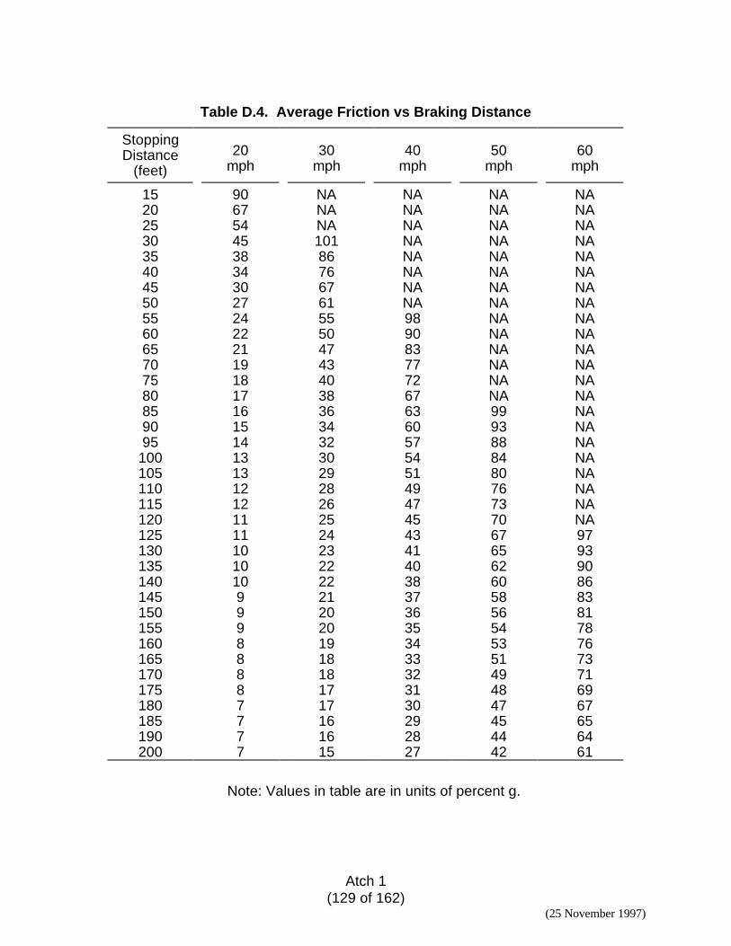
Atch 1(129 of 162)
(25 November 1997)
Table D.4. Average Friction vs Braking Distance
StoppingDistance
(feet)20
mph30
mph40
mph50
mph60
mph
15 90 NA NA NA NA20 67 NA NA NA NA25 54 NA NA NA NA30 45 101 NA NA NA35 38 86 NA NA NA40 34 76 NA NA NA45 30 67 NA NA NA50 27 61 NA NA NA55 24 55 98 NA NA60 22 50 90 NA NA65 21 47 83 NA NA70 19 43 77 NA NA75 18 40 72 NA NA80 17 38 67 NA NA85 16 36 63 99 NA90 15 34 60 93 NA95 14 32 57 88 NA
100 13 30 54 84 NA105 13 29 51 80 NA110 12 28 49 76 NA115 12 26 47 73 NA120 11 25 45 70 NA125 11 24 43 67 97130 10 23 41 65 93135 10 22 40 62 90140 10 22 38 60 86145 9 21 37 58 83150 9 20 36 56 81155 9 20 35 54 78160 8 19 34 53 76165 8 18 33 51 73170 8 18 32 49 71175 8 17 31 48 69180 7 17 30 47 67185 7 16 29 45 65190 7 16 28 44 64200 7 15 27 42 61
Note: Values in table are in units of percent g.
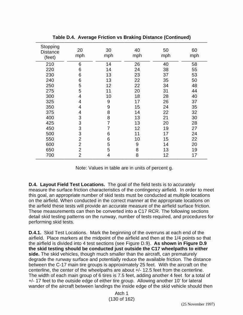
Atch 1(130 of 162)
(25 November 1997)
Table D.4. Average Friction vs Braking Distance (Continued)
StoppingDistance
(feet)
20mph
30mph
40mph
50mph
60mph
210 6 14 26 40 58220 6 14 24 38 55230 6 13 23 37 53240 6 13 22 35 50250 5 12 22 34 48275 5 11 20 31 44300 4 10 18 28 40325 4 9 17 26 37350 4 9 15 24 35375 4 8 14 22 32400 3 8 13 21 30425 3 7 13 20 28450 3 7 12 19 27500 3 6 11 17 24550 2 6 10 15 22600 2 5 9 14 20650 2 5 8 13 19700 2 4 8 12 17
Note: Values in table are in units of percent g.
D.4. Layout Field Test Locations. The goal of the field tests is to accuratelymeasure the surface friction characteristics of the contingency airfield. In order to meetthis goal, an appropriate number of skid tests must be conducted at multiple locationson the airfield. When conducted in the correct manner at the appropriate locations onthe airfield these tests will provide an accurate measure of the airfield surface friction.These measurements can then be converted into a C17 RCR. The following sectionsdetail skid testing patterns on the runway, number of tests required, and procedures forperforming skid tests.
D.4.1. Skid Test Locations. Mark the beginning of the overruns at each end of theairfield. Place markers at the midpoint of the airfield and then at the 1/4 points so thatthe airfield is divided into 4 test sections (see Figure D.9). As shown in Figure D.9the skid testing should be conducted just outside the C17 wheelpaths to eitherside. The skid vehicles, though much smaller than the aircraft, can prematurelydegrade the runway surface and potentially reduce the available friction. The distancebetween the C-17 main tire groups is approximately 25 feet. With the aircraft on thecenterline, the center of the wheelpaths are about +/- 12.5 feet from the centerline.The width of each main group of 6 tires is 7.5 feet, adding another 4 feet for a total of+/- 17 feet to the outside edge of either tire group. Allowing another 10' for lateralwander of the aircraft between landings the inside edge of the skid vehicle should then
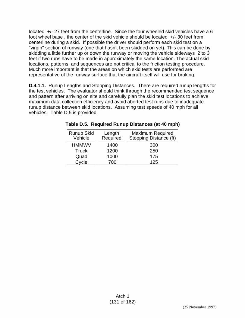
Atch 1(131 of 162)
(25 November 1997)
located +/- 27 feet from the centerline. Since the four wheeled skid vehicles have a 6foot wheel base , the center of the skid vehicle should be located +/- 30 feet fromcenterline during a skid. If possible the driver should perform each skid test on a"virgin" section of runway (one that hasn’t been skidded on yet). This can be done byskidding a little further up or down the runway or moving the vehicle sideways 2 to 3feet if two runs have to be made in approximately the same location. The actual skidlocations, patterns, and sequences are not critical to the friction testing procedure.Much more important is that the areas on which skid tests are performed arerepresentative of the runway surface that the aircraft itself will use for braking.
D.4.1.1. Runup Lengths and Stopping Distances. There are required runup lengths forthe test vehicles. The evaluator should think through the recommended test sequenceand pattern after arriving on site and carefully plan the skid test locations to achievemaximum data collection efficiency and avoid aborted test runs due to inadequaterunup distance between skid locations. Assuming test speeds of 40 mph for allvehicles, Table D.5 is provided.
Table D.5. Required Runup Distances (at 40 mph)
Runup SkidVehicle
LengthRequired
Maximum RequiredStopping Distance (ft)
HMMWV 1400 300Truck 1200 250Quad 1000 175Cycle 700 125
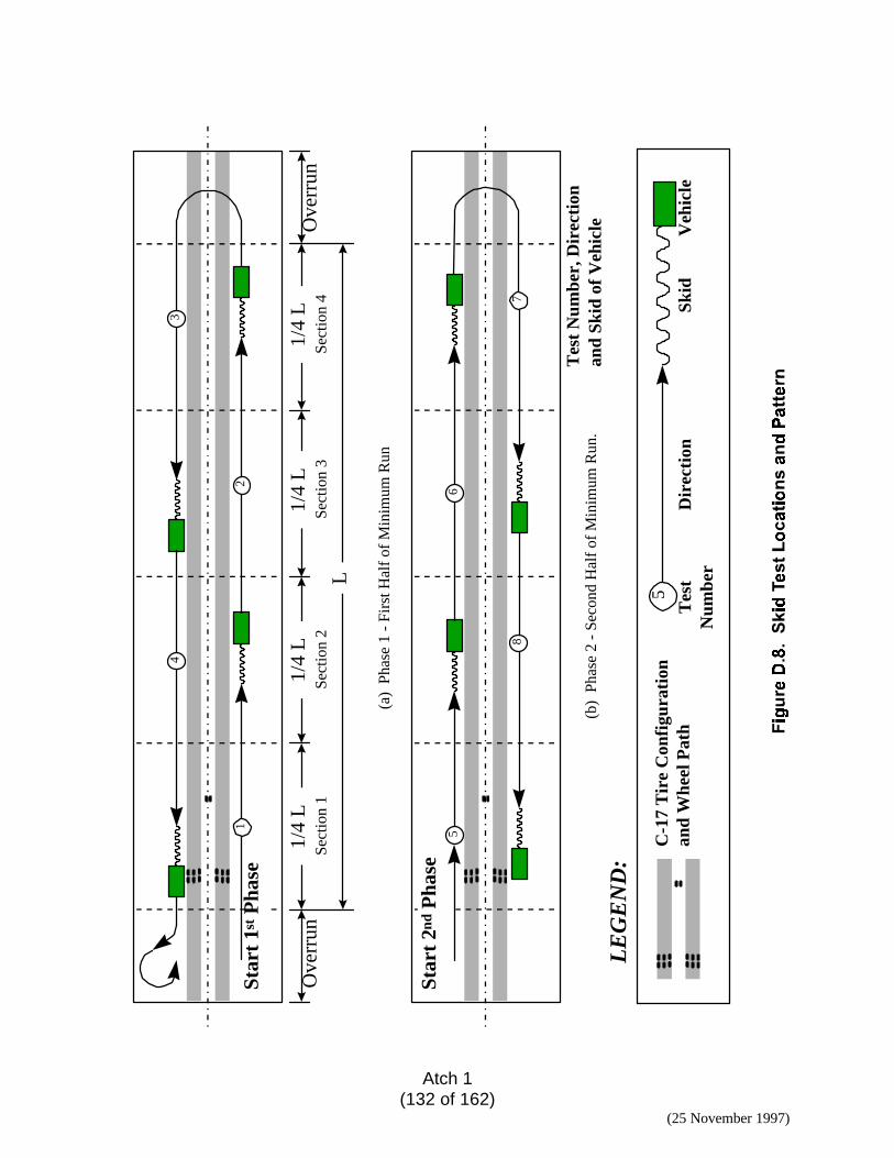
Atch 1(132 of 162)
(25 November 1997)
L
1/4
LSe
ctio
n 1
Ove
rrun
Ove
rrun
(a)
Pha
se 1
- F
irst
Hal
f of
Min
imum
Run
12
43
Star
t 1s
t Pha
se
6
87
(b)
Pha
se 2
- S
econ
d H
alf
of M
inim
um R
un.
C-1
7 T
ire
Con
figu
rati
onan
d W
heel
Pat
hT
est
Num
ber
5
LE
GE
ND
:
Star
t 2n
d P
hase
5
1/4
LSe
ctio
n 2
1/4
LSe
ctio
n 3
1/4
LSe
ctio
n 4
Tes
t N
umbe
r, D
irec
tion
and
Skid
of
Veh
icle
Dir
ecti
on
Skid
V
ehic
le
Atch 1(133 of 162)
(25 November 1997)
Note that if the approach ends of the runway provide extra runup room (in addition tothe 500-foot overruns), they can be used if they allow for smooth, uniform acceleration.Overruns can be used for vehicle acceleration but should not be used for skid testing.
D.4.2. Number of Tests Required. Preliminary analysis of the research data hasdetermined the number of tests required for a typical contingency airfield evaluation(4000'x90' as an example), as shown in Table D.5. Times shown in Table D.6 are onlyapproximate and can vary highly depending on vehicle type, vehicle condition, length ofrunway, driver technique, and data collection efficiency.
Table D.6. Number of Tests Required
Number of Tests Confidence Level Time to Complete
8 Minimum Required 20 minutes16 Standard 35 minutes
24 or more Desired 50 minutes or more
D.4.2.1. Minimum Number of Tests. The minimum number of tests required is 8. Theairfield evaluator should perform these tests in the approximate locations as shown inFigure D.9 . To perform this minimum number of tests the driver conducts skid tests 1through 4 at the locations shown in Figure D.9 (a). The driver then conducts skid tests5 through 8 at the locations shown in Figure D.9 (b). The skid locations shown withineach section are just guidelines. It is preferable to skid in the center of each section butif runway length or vehicle performance require skidding elsewhere that is acceptable,as long as a skid remains in the appropriate section. For extremely short runways thedriver may back the vehicle up after a skid to allow more runup distance for the nextskid.
D.4.1.2. Medium Confidence Level. A more accurate answer will result from theevaluator performing 16 tests. To perform this larger number of tests, conduct theprocedure described in Section D.4.2.1. twice; reversing direction on the second set.This insures that an even number of tests are conducted in either direction. This helpsto compensate for the effects of the wind on the friction measurements.
D.4.1.3. High Confidence Level. The most accurate results will be achieved if theevaluator has the time to perform 24 or more skid tests. The driver repeats the two testpatterns shown in Figure D.9 (reversing direction after each subset of 8 tests) until thetotal number of tests reaches the desired number. With the test pattern shown, 24 or32 tests can easily be performed. It is unnecessary to collect more than 32 tests.
D.5. Perform Skid Testing. The following section lists the general steps required toperform one friction test at one skid location. Any of the following items in bold areextremely important and must be followed for the test to be accurate.
Atch 1(134 of 162)
(25 November 1997)
1. Align test vehicle with runway on one of the two longitudinal test linesshown in Figure D.9. Both vehicle and tires should be straight.
2. Arm Bowmonk unit for test. Device should be armed just prior tovehicle acceleration. If unit is armed and a delay of more than 15seconds occurs, unit should be reset and then rearmed.
3. Begin vehicle acceleration smoothly but quickly. Acceleration shouldbe uniform without spinning tires or excessive vehicle bounce.Proceed down runway, accelerating uniformly to target test speed.
4. Once test speed has been reached, maintain uniform speed for 2 sec.
5. Perform skid test. Apply full-braking until coming to a completestop. Remember full rear braking only for quad and cycle.
6. Bring vehicle to a complete stop. Vehicle and driver MUST remainstill for several seconds while Bowmonk unit calculates andrecords braking information.
7. Check test results in the Bowmonk display.
8. If data appears valid, accept test. If data appears invalid reject andrepeat test.
10. Ready Bowmonk for next skid test.
If data appears invalid, reject test, return to previous starting location and repeat steps1 through 8. If vehicle is not properly aligned with the runway after skidding to a stop(wheels pointed straight ahead) then pull forward and align vehicle and wheels for nextskid. Several of the above steps are discussed in greater detail in the followingsections.
D.5.1.1. Target Speed at Braking. The following target speeds are recommended foroperational skid testing: 60 mph for the HMMWV and six pax, 50 mph for the quadand cycle. Please note that the cycle may not have a speedometer or tachometer, sothe operator must establish speed when using this test vehicle. If the cycle speed iscorrect to within +/- 10 mph an adequate deceleration value will be measured. With allvehicles, the driver should attempt to obtain correct target speed within reason.However, attempts to maintain proper speed should not override other considerationsdescribed in this appendix which are required to perform testing properly.
D.5.1.2. Braking Procedure. The correct braking procedure is to apply full braking untilcompletely stopped. For the HMMWV and six pax, this means pushing on thebrake pedal as hard as possible to lock up all four tires and then skidding to acomplete stop. For the cycle and quad, it is unsafe to lock up both the front andback brakes so the procedure requires locking up the back brakes only. Full-braking must be used for operational testing. Note: Warm up test skids should beperformed, starting at lower test speeds and using non-skid braking (partial braking) toconfirm proper braking action and determine vehicle braking behavior at the particularairfield.
Atch 1(135 of 162)
(25 November 1997)
D.5.1.3. Steering During Skids. During the skids, a nominal amount of steering will berequired to maintain as straight a line as possible. This is acceptable and will notsignificantly affect the test results. If the vehicle twists more than +/- 15 degreesfrom a longitudinal line, then the test must be repeated.
D.6. Calculate C-17 RCR. There are three ways to calculate the Runway ConditionRating (RCR) value required for C-17 contingency operations:
− Convert Bowmonk “Mean Deceleration” readings into RCR− Convert Soil Type to RCR− Convert Ground Vehicle Skid Distance Measurements to RCR
D.6.1. Convert Bowmonk “Mean Deceleration” Readings into Aircraft RCR Values.This section describes the first method, which is by far the most accurate. Datacollected with the Bowmonk can be used in Table D.7 to convert the frictionmeasurements into an equivalent C17 RCR. The mean deceleration measurementsare used to calculate an overall average mean value. This average value is comparedto the values in column two (mean) and the appropriate C17 RCR value is determined.
D.6.2. Alternate Friction Prediction Procedures. There are two alternate frictionprediction procedures: correlating the soil type to RCR, and directly measuring the skiddistance with a ground vehicle and correlating to RCR. Of the two alternateprocedures, measuring the skid distance is more accurate, and is preferred overcorrelating RCR to soil type only.
Table D.7. Stopping Friction Guidance (Preliminary)
Semi-PreparedRunway
Surface ConditionHUMVEEBowmonkReading
(at 40 mph)*
RCR
Unstabilized Visibly dry, dry depth 2” >61 20Cement Stabilized Visibly dry, no puddles >61 20
Either Damp to wet N/A 4
Note: Average of all eight “mean decel (in %g) readings.
Table D.8. Correlation Between Soil Type and RCR
Soil TypeUSCS
ClassificationWater
Content C-17 RCR
Well Graded Gravels GW Dry 20Clean Sands (< 5% fines) SW, SP Dry 22Clayey Sands, Silty Sands (>12% fines) SC, SM Dry 22Low Plasticity Clays & Silts CL, ML Dry 23
Atch 1(136 of 162)
(25 November 1997)
D.6.2.1. Mean Deceleration Measurements from Measured Skid Distance. If aBowmonk unit is not available or if the unit should malfunction in the field, thisprocedure can be used to obtain an RCR value. The skidding and distancemeasurement procedure as described in the operational paragraph D.3.5.6,"Verification by Direct Measurement of Skid Distance," should be followed. Actual skidtests should be conducted in the number described in paragraph D.4.2, "Number ofTests Required," and in the test patterns shown in Figure D.9. Skidding tests shouldbe conducted as described in paragraph D.5, "Performing Skid Test." Skid speeds of40 mph should be used. Once testing is complete each skid distance measurement isconverted to a mean deceleration value as described in paragraph D.3.5.6,"Verification by Direct Measurement of Skid Distance," and shown in Table D.4. Theoverall average for these mean deceleration values is then calculated. This averagemean value is compared to column three of Table D.7 to determine the equivalent C-17RCR value.
D.6.2.2. Correlation with Soil Type/Classification. In lieu of collecting any actual skidtest data on the airfield surface, the characteristic friction parameter (RCR) may beestimated based on soil type and classification or strength data collected to assess thestructural suitability of the airfield. This method is the least accurate and should only beused as a last resort. Appendix A provides the soil test methods that should be used todetermine the soil type in the field. Table D.8 provides the correlation used to estimateRCR.
D.7. Rolling Friction Estimation. The rolling friction factor is important when theunsurfaced airfield is soft enough to produce appreciable loose till. The aircraft must“plow” through this loose till and this produces a requirement for slightly longer takeoffdistances. This loose till depth should be measured at five locations on the runway inaccordance with the measuring procedures described in Appendix B. Suggestedmeasurement locations include; touchdown area, initial braking zone, point of rotation,departure end of runway, and other areas where the surface may be softened due topoor drainage, improper construction, aircraft turning, etc. Calculate the average ofthese five till depth measurements to establish the overall runway till depth, then referto Table D.9 to determine the approximate rolling friction factor for the runway surfacemeasured.
Table D.9. Rolling Friction Guidance
Semi-preparedRunway
Dry Till Depth Rolling Friction Factor
Unstabilized (dry) 0 to 1.5 inches 51.51 to 3.5 inches 10
3.51 to 5.75 inches 155.76 to 7.75 inches 20
>7.75 inches Maintenance RequiredUnstabilized (damp to wet) 0 to 1.0 inches 5
Cement stabilized 0 to 0.5 inches 2

Atch 1(137 of 162)
(25 November 1997)
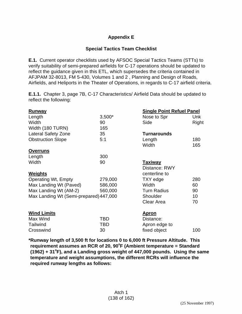
Atch 1(138 of 162)
(25 November 1997)
Appendix E
Special Tactics Team Checklist
E.1. Current operator checklists used by AFSOC Special Tactics Teams (STTs) toverify suitability of semi-prepared airfields for C-17 operations should be updated toreflect the guidance given in this ETL, which supersedes the criteria contained inAFJPAM 32-8013, FM 5-430, Volumes 1 and 2 , Planning and Design of Roads,Airfields, and Heliports in the Theater of Operations, in regards to C-17 airfield criteria.
E.1.1. Chapter 3, page 7B, C-17 Characteristics/ Airfield Data should be updated toreflect the following:
Runway Single Point Refuel PanelLength 3,500* Nose to Spr UnkWidth 90 Side RightWidth (180 TURN) 165Lateral Safety Zone 35 TurnaroundsObstruction Slope 5:1 Length 180
Width 165OverrunsLength 300Width 90 Taxiway
Distance: RWYWeights centerline toOperating Wt, Empty 279,000 TXY edge 280Max Landing Wt (Paved) 586,000 Width 60Max Landing Wt (AM-2) 560,000 Turn Radius 90Max Landing Wt (Semi-prepared)447,000 Shoulder 10
Clear Area 70
Wind Limits ApronMax Wind TBD Distance:Tailwind TBD Apron edge toCrosswind 30 fixed object 100
*Runway length of 3,500 ft for locations 0 to 6,000 ft Pressure Altitude. Thisrequirement assumes an RCR of 20, 90oF (Ambient temperature = Standard(1962) + 31oF), and a Landing gross weight of 447,000 pounds. Using the sametemperature and weight assumptions, the different RCRs will influence therequired runway lengths as follows:
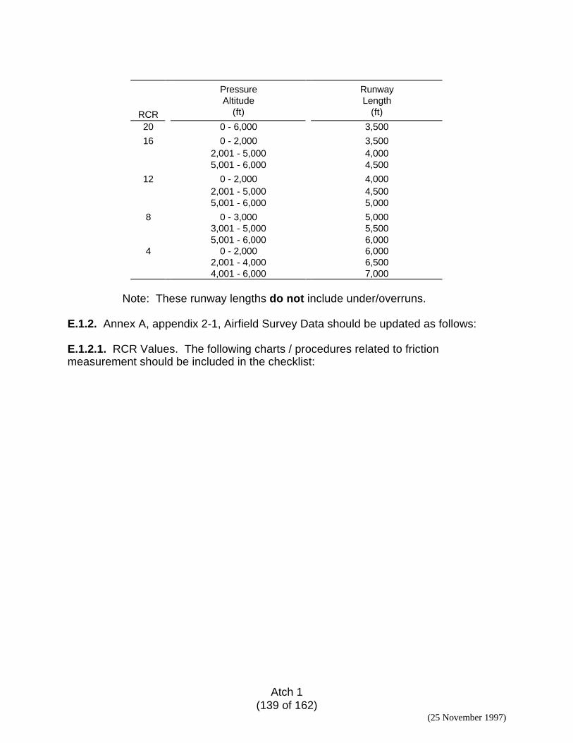
Atch 1(139 of 162)
(25 November 1997)
RCR
PressureAltitude
(ft)
RunwayLength
(ft)
20 0 - 6,000 3,500
16 0 - 2,000 3,5002,001 - 5,000 4,0005,001 - 6,000 4,500
12 0 - 2,000 4,0002,001 - 5,000 4,5005,001 - 6,000 5,000
8 0 - 3,000 5,0003,001 - 5,000 5,500
45,001 - 6,000
0 - 2,0002,001 - 4,0004,001 - 6,000
6,0006,0006,5007,000
Note: These runway lengths do not include under/overruns.
E.1.2. Annex A, appendix 2-1, Airfield Survey Data should be updated as follows:
E.1.2.1. RCR Values. The following charts / procedures related to frictionmeasurement should be included in the checklist:
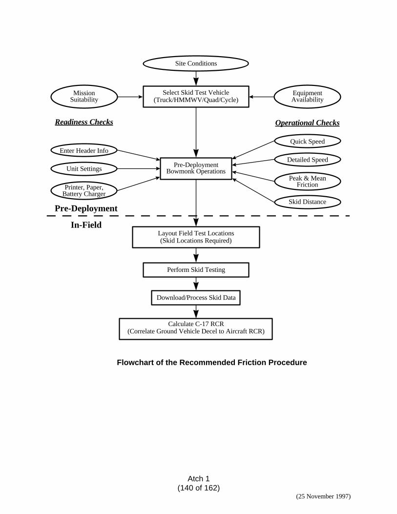
Atch 1(140 of 162)
(25 November 1997)
Pre-DeploymentBowmonk Operations
Select Skid Test Vehicle(Truck/HMMWV/Quad/Cycle)
MissionSuitability
Site Conditions
Perform Skid Testing
Download/Process Skid Data
Layout Field Test Locations(Skid Locations Required)
Calculate C-17 RCR(Correlate Ground Vehicle Decel to Aircraft RCR)
EquipmentAvailability
Readiness Checks
Enter Header Info
Unit Settings
Printer, Paper,Battery Charger
Operational Checks
Quick Speed
Detailed Speed
Peak & MeanFriction
Skid DistancePre-Deployment
In-Field
Flowchart of the Recommended Friction Procedure
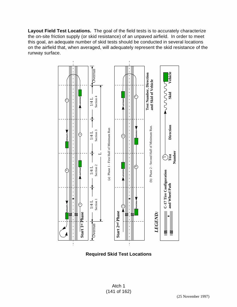
Atch 1(141 of 162)
(25 November 1997)
Layout Field Test Locations. The goal of the field tests is to accurately characterizethe on-site friction supply (or skid resistance) of an unpaved airfield. In order to meetthis goal, an adequate number of skid tests should be conducted in several locationson the airfield that, when averaged, will adequately represent the skid resistance of therunway surface.
L
1/4
LSe
ctio
n 1
Ove
rrun
Ove
rrun
(a)
Pha
se 1
- F
irst
Hal
f of
Min
imum
Run
12
43
Star
t 1s
t Pha
se
6
87
(b)
Pha
se 2
- S
econ
d H
alf
of M
inim
um R
un.
C-1
7 T
ire
Con
figu
rati
onan
d W
heel
Pat
hT
est
Num
ber
5
LE
GE
ND
:
Star
t 2n
d P
hase
5
1/4
LSe
ctio
n 2
1/4
LSe
ctio
n 3
1/4
LSe
ctio
n 4
Tes
t N
umbe
r, D
irec
tion
and
Skid
of
Veh
icle
Dir
ecti
on
Skid
V
ehic
le
Required Skid Test Locations
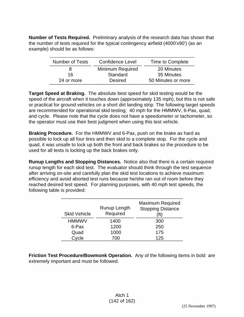
Atch 1(142 of 162)
(25 November 1997)
Number of Tests Required. Preliminary analysis of the research data has shown thatthe number of tests required for the typical contingency airfield (4000'x90') (as anexample) should be as follows:
Number of Tests Confidence Level Time to Complete
8 Minimum Required 20 Minutes16 Standard 35 Minutes
24 or more Desired 50 Minutes or more
Target Speed at Braking. The absolute best speed for skid testing would be thespeed of the aircraft when it touches down (approximately 135 mph), but this is not safeor practical for ground vehicles on a short dirt landing strip. The following target speedsare recommended for operational skid testing; 40 mph for the HMMWV, 6-Pax, quad,and cycle. Please note that the cycle does not have a speedometer or tachometer, sothe operator must use their best judgment when using this test vehicle.
Braking Procedure. For the HMMWV and 6-Pax, push on the brake as hard aspossible to lock up all four tires and then skid to a complete stop. For the cycle andquad, it was unsafe to lock up both the front and back brakes so the procedure to beused for all tests is locking up the back brakes only.
Runup Lengths and Stopping Distances. Notice also that there is a certain requiredrunup length for each skid test. The evaluator should think through the test sequenceafter arriving on-site and carefully plan the skid test locations to achieve maximumefficiency and avoid aborted test runs because he/she ran out of room before theyreached desired test speed. For planning purposes, with 40 mph test speeds, thefollowing table is provided:
Skid VehicleRunup Length
Required
Maximum RequiredStopping Distance
(ft)HMMWV 1400 300
6-Pax 1200 250Quad 1000 175Cycle 700 125
Friction Test Procedure/Bowmonk Operation. Any of the following items in bold areextremely important and must be followed.
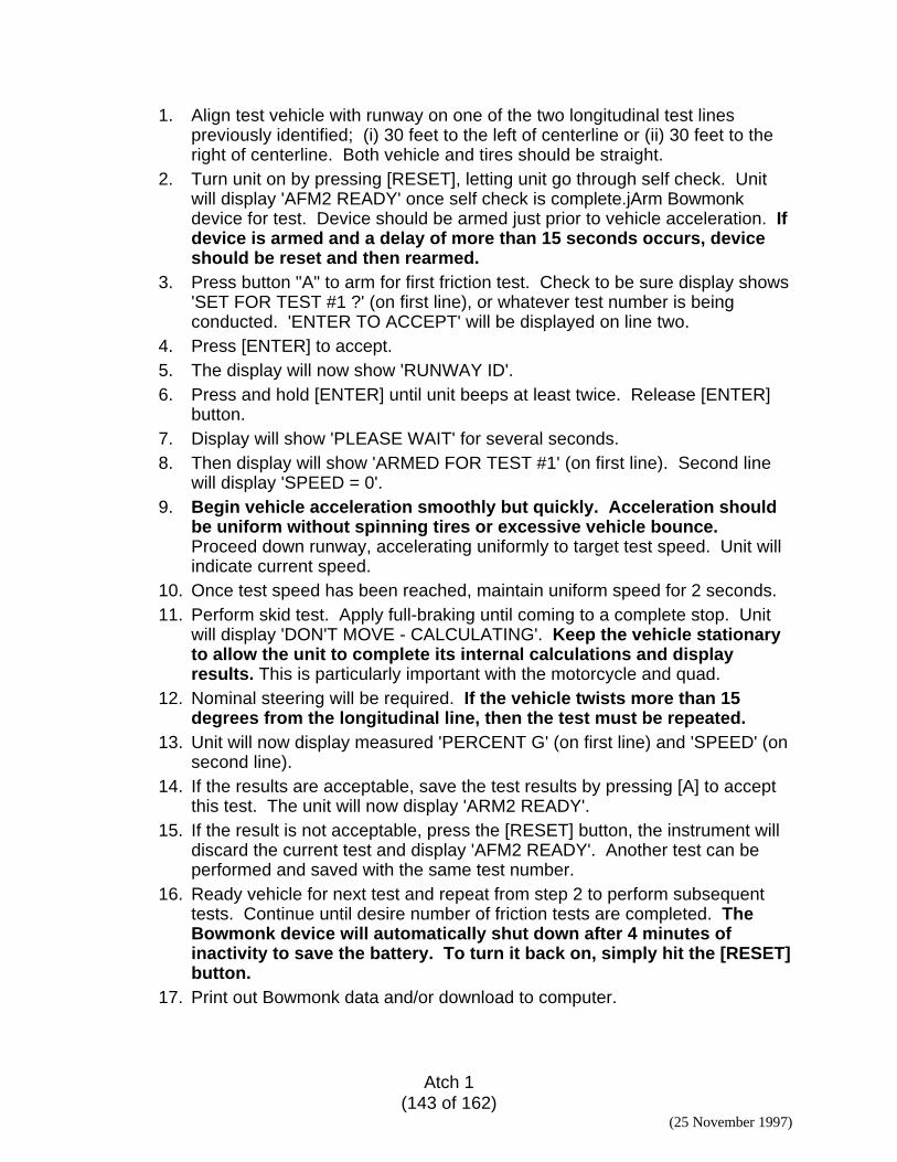
Atch 1(143 of 162)
(25 November 1997)
1. Align test vehicle with runway on one of the two longitudinal test linespreviously identified; (i) 30 feet to the left of centerline or (ii) 30 feet to theright of centerline. Both vehicle and tires should be straight.
2. Turn unit on by pressing [RESET], letting unit go through self check. Unitwill display 'AFM2 READY' once self check is complete.jArm Bowmonkdevice for test. Device should be armed just prior to vehicle acceleration. Ifdevice is armed and a delay of more than 15 seconds occurs, deviceshould be reset and then rearmed.
3. Press button "A" to arm for first friction test. Check to be sure display shows'SET FOR TEST #1 ?' (on first line), or whatever test number is beingconducted. 'ENTER TO ACCEPT' will be displayed on line two.
4. Press [ENTER] to accept.5. The display will now show 'RUNWAY ID'.6. Press and hold [ENTER] until unit beeps at least twice. Release [ENTER]
button.7. Display will show 'PLEASE WAIT' for several seconds.8. Then display will show 'ARMED FOR TEST #1' (on first line). Second line
will display 'SPEED = 0'.9. Begin vehicle acceleration smoothly but quickly. Acceleration should
be uniform without spinning tires or excessive vehicle bounce.Proceed down runway, accelerating uniformly to target test speed. Unit willindicate current speed.
10. Once test speed has been reached, maintain uniform speed for 2 seconds.11. Perform skid test. Apply full-braking until coming to a complete stop. Unit
will display 'DON'T MOVE - CALCULATING'. Keep the vehicle stationaryto allow the unit to complete its internal calculations and displayresults. This is particularly important with the motorcycle and quad.
12. Nominal steering will be required. If the vehicle twists more than 15degrees from the longitudinal line, then the test must be repeated.
13. Unit will now display measured 'PERCENT G' (on first line) and 'SPEED' (onsecond line).
14. If the results are acceptable, save the test results by pressing [A] to acceptthis test. The unit will now display 'ARM2 READY'.
15. If the result is not acceptable, press the [RESET] button, the instrument willdiscard the current test and display 'AFM2 READY'. Another test can beperformed and saved with the same test number.
16. Ready vehicle for next test and repeat from step 2 to perform subsequenttests. Continue until desire number of friction tests are completed. TheBowmonk device will automatically shut down after 4 minutes ofinactivity to save the battery. To turn it back on, simply hit the [RESET]button.
17. Print out Bowmonk data and/or download to computer.
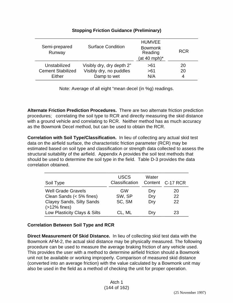
Atch 1(144 of 162)
(25 November 1997)
Stopping Friction Guidance (Preliminary)
Semi-preparedRunway
Surface ConditionHUMVEEBowmonkReading
(at 40 mph)*
RCR
Unstabilized Visibly dry, dry depth 2” >61 20Cement Stabilized Visibly dry, no puddles >61 20
Either Damp to wet N/A 4
Note: Average of all eight “mean decel (in %g) readings.
Alternate Friction Prediction Procedures. There are two alternate friction predictionprocedures; correlating the soil type to RCR and directly measuring the skid distancewith a ground vehicle and correlating to RCR. Neither method has as much accuracyas the Bowmonk Decel method, but can be used to obtain the RCR.
Correlation with Soil Type/Classification. In lieu of collecting any actual skid testdata on the airfield surface, the characteristic friction parameter (RCR) may beestimated based on soil type and classification or strength data collected to assess thestructural suitability of the airfield. Appendix A provides the soil test methods thatshould be used to determine the soil type in the field. Table D-3 provides the datacorrelation obtained.
Soil TypeUSCS
ClassificationWater
Content C-17 RCR
Well Grade Gravels GW Dry 20Clean Sands (< 5% fines) SW, SP Dry 22Clayey Sands, Silty Sands(>12% fines)
SC, SM Dry 22
Low Plasticity Clays & Silts CL, ML Dry 23
Correlation Between Soil Type and RCR
Direct Measurement Of Skid Distance. In lieu of collecting skid test data with theBowmonk AFM-2, the actual skid distance may be physically measured. The followingprocedure can be used to measure the average braking friction of any vehicle used.This provides the user with a method to determine airfield friction should a Bowmonkunit not be available or working improperly. Comparison of measured skid distance(converted into an average friction) with the value calculated by a Bowmonk unit mayalso be used in the field as a method of checking the unit for proper operation.
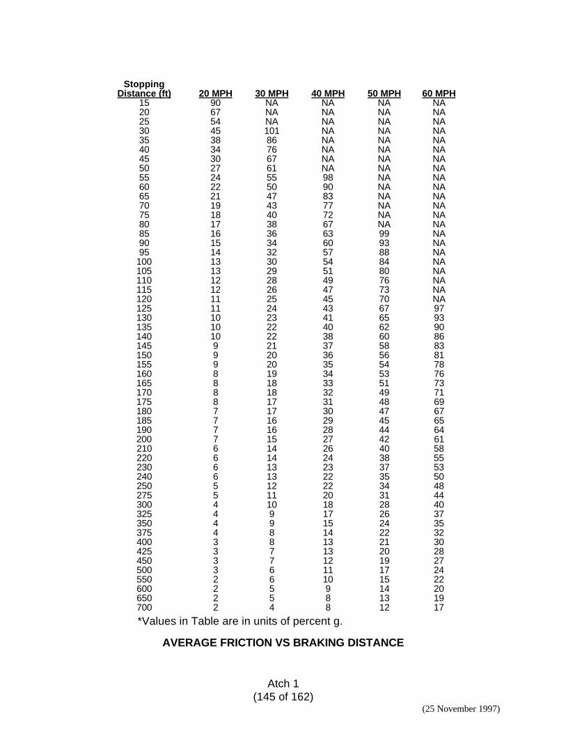
Atch 1(145 of 162)
(25 November 1997)
StoppingDistance (ft) 20 MPH 30 MPH 40 MPH 50 MPH 60 MPH
15 90 NA NA NA NA20 67 NA NA NA NA25 54 NA NA NA NA30 45 101 NA NA NA35 38 86 NA NA NA40 34 76 NA NA NA45 30 67 NA NA NA50 27 61 NA NA NA55 24 55 98 NA NA60 22 50 90 NA NA65 21 47 83 NA NA70 19 43 77 NA NA75 18 40 72 NA NA80 17 38 67 NA NA85 16 36 63 99 NA90 15 34 60 93 NA95 14 32 57 88 NA
100 13 30 54 84 NA105 13 29 51 80 NA110 12 28 49 76 NA115 12 26 47 73 NA120 11 25 45 70 NA125 11 24 43 67 97130 10 23 41 65 93135 10 22 40 62 90140 10 22 38 60 86145 9 21 37 58 83150 9 20 36 56 81155 9 20 35 54 78160 8 19 34 53 76165 8 18 33 51 73170 8 18 32 49 71175 8 17 31 48 69180 7 17 30 47 67185 7 16 29 45 65190 7 16 28 44 64200 7 15 27 42 61210 6 14 26 40 58220 6 14 24 38 55230 6 13 23 37 53240 6 13 22 35 50250 5 12 22 34 48275 5 11 20 31 44300 4 10 18 28 40325 4 9 17 26 37350 4 9 15 24 35375 4 8 14 22 32400 3 8 13 21 30425 3 7 13 20 28450 3 7 12 19 27500 3 6 11 17 24550 2 6 10 15 22600 2 5 9 14 20650 2 5 8 13 19700 2 4 8 12 17
*Values in Table are in units of percent g.
AVERAGE FRICTION VS BRAKING DISTANCE
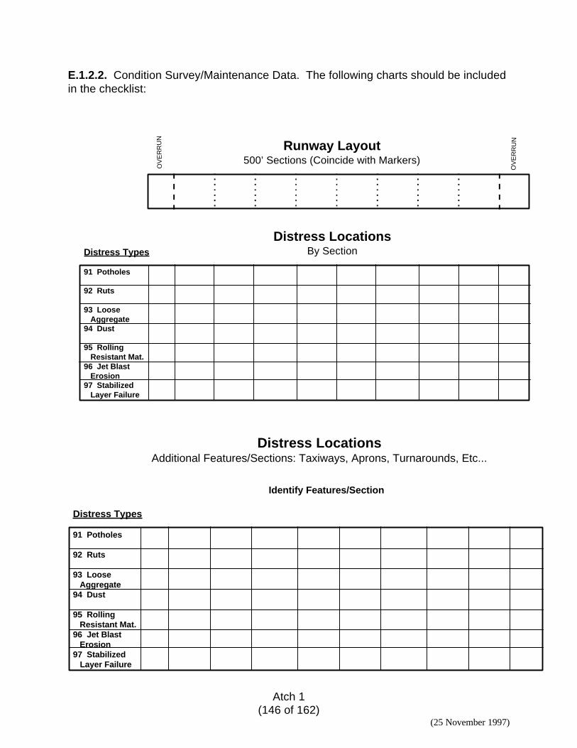
Atch 1(146 of 162)
(25 November 1997)
E.1.2.2. Condition Survey/Maintenance Data. The following charts should be includedin the checklist:
Runway Layout500’ Sections (Coincide with Markers)
OV
ER
RU
N
OV
ER
RU
N
Distress LocationsBy SectionDistress Types
91 Potholes
92 Ruts
93 Loose Aggregate94 Dust
95 Rolling Resistant Mat.96 Jet Blast Erosion97 Stabilized Layer Failure
Distress LocationsAdditional Features/Sections: Taxiways, Aprons, Turnarounds, Etc...
Identify Features/Section
Distress Types
91 Potholes
92 Ruts
93 Loose Aggregate94 Dust
95 Rolling Resistant Mat.96 Jet Blast Erosion97 Stabilized Layer Failure
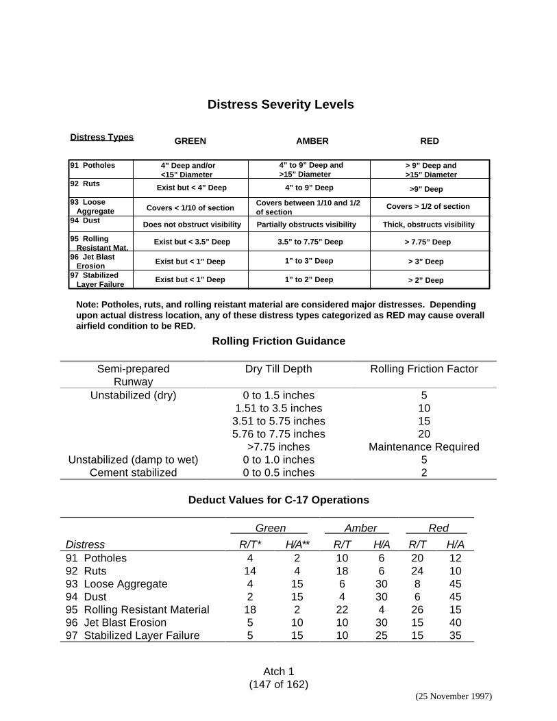
Atch 1(147 of 162)
(25 November 1997)
Distress Severity Levels
Distress Types
91 Potholes
92 Ruts
93 Loose Aggregate94 Dust
95 Rolling Resistant Mat.96 Jet Blast Erosion97 Stabilized Layer Failure
GREEN AMBER RED
4” Deep and/or<15” Diameter
4” to 9” Deep and>15” Diameter
> 9” Deep and>15” Diameter
Exist but < 4” Deep 4” to 9” Deep >9” Deep
Covers < 1/10 of sectionCovers between 1/10 and 1/2 of section
Covers > 1/2 of section
Does not obstruct visibility Partially obstructs visibility Thick, obstructs visibility
Exist but < 3.5” Deep 3.5” to 7.75” Deep > 7.75” Deep
Exist but < 1” Deep 1” to 3” Deep > 3” Deep
Exist but < 1” Deep 1” to 2” Deep > 2” Deep
Note: Potholes, ruts, and rolling reistant material are considered major distresses. Depending upon actual distress location, any of these distress types categorized as RED may cause overall airfield condition to be RED.
Rolling Friction Guidance
Semi-preparedRunway
Dry Till Depth Rolling Friction Factor
Unstabilized (dry) 0 to 1.5 inches 51.51 to 3.5 inches 10
3.51 to 5.75 inches 155.76 to 7.75 inches 20
>7.75 inches Maintenance RequiredUnstabilized (damp to wet) 0 to 1.0 inches 5
Cement stabilized 0 to 0.5 inches 2
Deduct Values for C-17 Operations
Green Amber Red
Distress R/T* H/A** R/T H/A R/T H/A91 Potholes 4 2 10 6 20 1292 Ruts 14 4 18 6 24 1093 Loose Aggregate 4 15 6 30 8 4594 Dust 2 15 4 30 6 4595 Rolling Resistant Material 18 2 22 4 26 1596 Jet Blast Erosion 5 10 10 30 15 4097 Stabilized Layer Failure 5 15 10 25 15 35
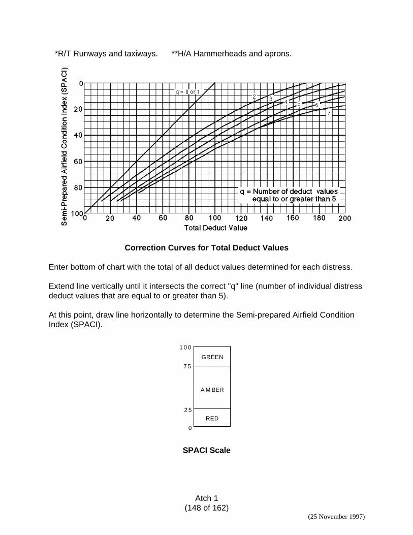
Atch 1(148 of 162)
(25 November 1997)
*R/T Runways and taxiways. **H/A Hammerheads and aprons.
Correction Curves for Total Deduct Values
Enter bottom of chart with the total of all deduct values determined for each distress.
Extend line vertically until it intersects the correct "q" line (number of individual distressdeduct values that are equal to or greater than 5).
At this point, draw line horizontally to determine the Semi-prepared Airfield ConditionIndex (SPACI).
GREEN
A M BER
RED
1 0 0
7 5
2 5
0
SPACI Scale
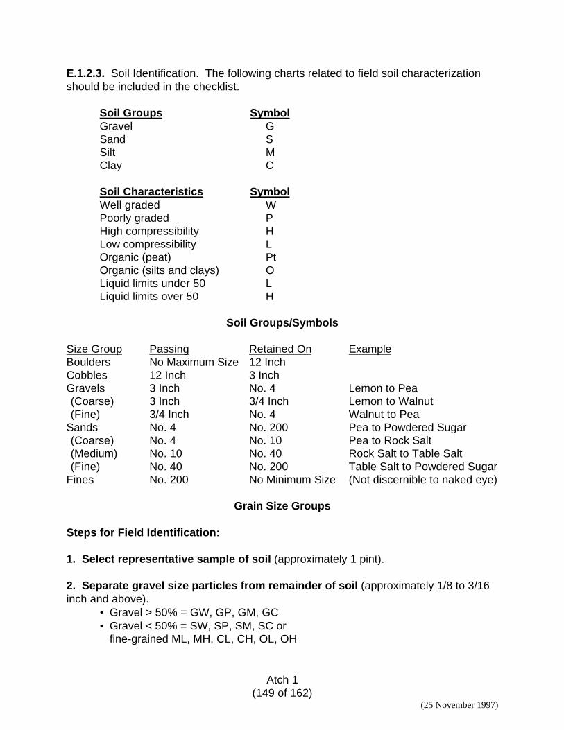
Atch 1(149 of 162)
(25 November 1997)
E.1.2.3. Soil Identification. The following charts related to field soil characterizationshould be included in the checklist.
Soil Groups SymbolGravel GSand SSilt MClay C
Soil Characteristics SymbolWell graded WPoorly graded PHigh compressibility HLow compressibility LOrganic (peat) PtOrganic (silts and clays) OLiquid limits under 50 LLiquid limits over 50 H
Soil Groups/Symbols
Size Group Passing Retained On ExampleBoulders No Maximum Size 12 InchCobbles 12 Inch 3 InchGravels 3 Inch No. 4 Lemon to Pea(Coarse) 3 Inch 3/4 Inch Lemon to Walnut(Fine) 3/4 Inch No. 4 Walnut to Pea
Sands No. 4 No. 200 Pea to Powdered Sugar(Coarse) No. 4 No. 10 Pea to Rock Salt(Medium) No. 10 No. 40 Rock Salt to Table Salt(Fine) No. 40 No. 200 Table Salt to Powdered Sugar
Fines No. 200 No Minimum Size (Not discernible to naked eye)
Grain Size Groups
Steps for Field Identification:
1. Select representative sample of soil (approximately 1 pint).
2. Separate gravel size particles from remainder of soil (approximately 1/8 to 3/16inch and above).
• Gravel > 50% = GW, GP, GM, GC• Gravel < 50% = SW, SP, SM, SC or
fine-grained ML, MH, CL, CH, OL, OH
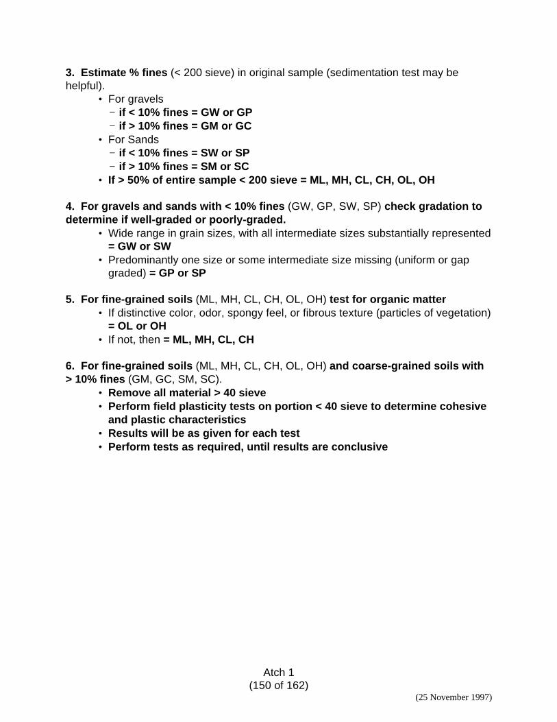
Atch 1(150 of 162)
(25 November 1997)
3. Estimate % fines (< 200 sieve) in original sample (sedimentation test may behelpful).
• For gravels− if < 10% fines = GW or GP− if > 10% fines = GM or GC
• For Sands− if < 10% fines = SW or SP− if > 10% fines = SM or SC
• If > 50% of entire sample < 200 sieve = ML, MH, CL, CH, OL, OH
4. For gravels and sands with < 10% fines (GW, GP, SW, SP) check gradation todetermine if well-graded or poorly-graded.
• Wide range in grain sizes, with all intermediate sizes substantially represented= GW or SW
• Predominantly one size or some intermediate size missing (uniform or gapgraded) = GP or SP
5. For fine-grained soils (ML, MH, CL, CH, OL, OH) test for organic matter• If distinctive color, odor, spongy feel, or fibrous texture (particles of vegetation)
= OL or OH• If not, then = ML, MH, CL, CH
6. For fine-grained soils (ML, MH, CL, CH, OL, OH) and coarse-grained soils with> 10% fines (GM, GC, SM, SC).
• Remove all material > 40 sieve• Perform field plasticity tests on portion < 40 sieve to determine cohesive
and plastic characteristics• Results will be as given for each test• Perform tests as required, until results are conclusive
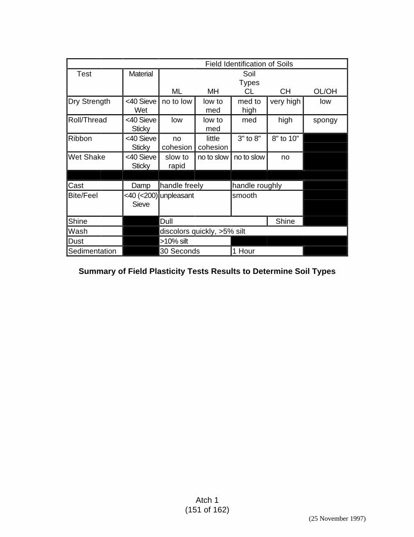
Atch 1(151 of 162)
(25 November 1997)
Field Identification of SoilsTest Material Soil
TypesML MH CL CH OL/OH
Dry Strength <40 SieveWet
no to low low tomed
med tohigh
very high low
Roll/Thread <40 SieveSticky
low low tomed
med high spongy
Ribbon <40 SieveSticky
nocohesion
littlecohesion
3" to 8" 8" to 10"
Wet Shake <40 SieveSticky
slow torapid
no to slow no to slow no
Cast Damp handle freely handle roughlyBite/Feel <40 (<200)
Sieveunpleasant smooth
Shine Dull ShineWash discolors quickly, >5% siltDust >10% siltSedimentation 30 Seconds 1 Hour
Summary of Field Plasticity Tests Results to Determine Soil Types
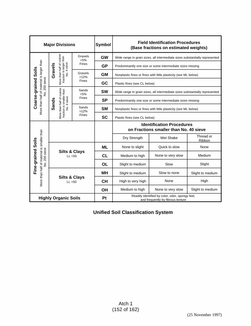
Atch 1(152 of 162)
(25 November 1997)
Major Divisions Symbol Field Identification Procedures(Base fractions on estimated weights)
GW
GP
GM
GC
SW
SP
SM
SC
ML
CL
OL
MH
CH
OH
Pt
Gravels<5%Fines
Sands<5%Fines
Sands>12%Fines
Gravels>12%Fines
Silts & ClaysLL <50
Silts & ClaysLL >50
Highly Organic Soils
Fin
e-g
rain
ed S
oils
Co
arse
-gra
ined
So
ils
Gra
vels
San
ds
Mor
e th
an h
alf o
f coa
rse
frac
tion
is la
rger
than
No.
4 s
ieve
Mor
e th
an h
alf o
f coa
rse
frac
tion
is s
mal
ler
than
No.
4 s
ieve
Mor
e th
an h
alf o
f mat
eria
l is
larg
er th
an
No.
200
sie
veM
ore
than
hal
f of m
ater
ial i
s sm
alle
r th
an
No.
200
sie
ve
Readily identified by color, odor, spongy feel,and frequently by fibrous texture
Wide range in grain sizes, all intermediate sizes substantially represented
Nonplastic fines or fines with little plasticity (see ML below)
Plastic fines (see CL below)
Wide range in grain sizes, all intermediate sizes substantially represented
Predominantly one size or some intermediate sizes missing
Nonplastic fines or fines with little plasticity (see ML below)
Plastic fines (see CL below)
Identification Procedureson Fractions smaller than No. 40 sieve
Predominantly one size or some intermediate sizes missing
Dry Strength Wet Shake Thread orRibbon
None to slight
Medium to high
Slight to medium
Slight to medium
High to very high
Medium to high
Quick to slow
None to very slow
Slow
Slow to none
None
None to very slow
None
Medium
Slight
Slight to medium
High
Slight to medium
Unified Soil Classification System
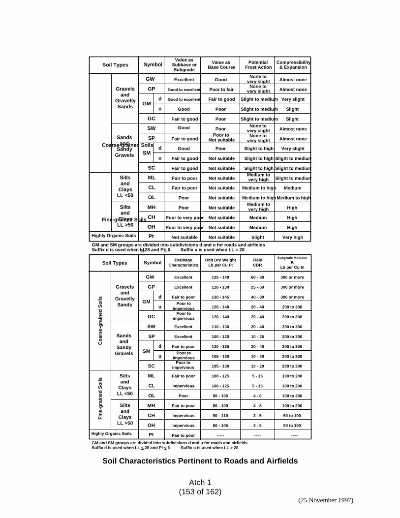
Atch 1(153 of 162)
(25 November 1997)
Soil Types Symbol
GW
GP
GM
GC
SW
SP
SM
SC
ML
CL
OL
MH
CH
OH
Pt
Siltsand
ClaysLL <50
Siltsand
ClaysLL >50
Highly Organic Soils
Fine-grained Soils
Coarse-grained Soils
Gravelsand
GravellySands
Sandsand
SandyGravels
d
u
d
u
GM and SM groups are divided into subdivisions d and u for roads and airfieldsSuffix d is used when LL< 28 and PI< 6 Suffix u is used when LL > 28
Value asSubbase orSubgrade
Value asBase Course
PotentialFrost Action
Compressibility& Expansion
Excellent
Good to excellent
Good to excellent
Good
Good
Good
Good
Fair to good
Fair to good
Fair to good
Fair to good
Fair to good
Fair to poor
Fair to poor
Poor
Poor
Poor
Poor
Poor
Poor
Poor to fair
Poor toNot suitable
Not suitable
Not suitable
Not suitable
Not suitable Not suitable
Not suitable
Not suitable
Not suitable
Not suitable
Not suitable
Poor to very poor
Poor to very poor
None tovery slightNone to
very slight
None tovery slightNone to
very slight
Slight to medium
Slight to medium
Slight to medium
Slight to medium
Slight to medium
Slight to medium
Slight to high
Slight to high
Slight to highMedium tovery high
Medium tovery high
Medium to high
Medium to highMedium to high
Medium
Medium
Medium
Slight
Slight
Slight
Almost none
Almost none
Almost none
Almost none
Very slight
Very slight
High
High
High
Very high
Soil Types Symbol
GW
GP
GM
GC
SW
SP
SM
SC
ML
CL
OL
MH
CH
OH
Pt
Siltsand
ClaysLL <50
Siltsand
ClaysLL >50
Highly Organic Soils
Fin
e-g
rain
ed S
oils
Co
arse
-gra
ined
So
ils
Gravelsand
GravellySands
Sandsand
SandyGravels
d
u
d
u
GM and SM groups are divided into subdivisions d and u for roads and airfieldsSuffix d is used when LL < 28 and PI < 6 Suffix u is used when LL > 28
DrainageCharacteristics
Unit Dry WeightLb per Cu Ft
FieldCBR
Subgrade ModulusK
Lb per Cu In
Excellent
Excellent
Excellent
Excellent
Fair to poor
Fair to poor
Fair to poor
Fair to poor
Fair to poor ----- ----- -----
Impervious
Impervious
Impervious
Poor
Poor toimpervious
Poor toimpervious
Poor toimpervious
Poor toimpervious
125 - 140
110 - 130
130 - 145
120 - 140
120 - 140
110 - 130
100 - 120
120 - 135
105 - 130
105 - 130
60 - 80
25 - 60
40 - 80
20 - 40
20 - 40
20 - 40
10 - 25
20 - 40
10 - 20
10 - 20
300 or more
300 or more
300 or more
200 to 300
200 to 300
200 to 300
200 to 300
200 to 300
200 to 300
200 to 300
100 to 200
100 to 200
100 to 200
100 to 200
50 to 100
50 to 100
100 - 125
100 - 125
90 - 105
90 - 110
80 - 105
80 - 100
5 - 15
5 - 15
4 - 8
4 - 8
3 - 5
3 - 5
Soil Characteristics Pertinent to Roads and Airfields
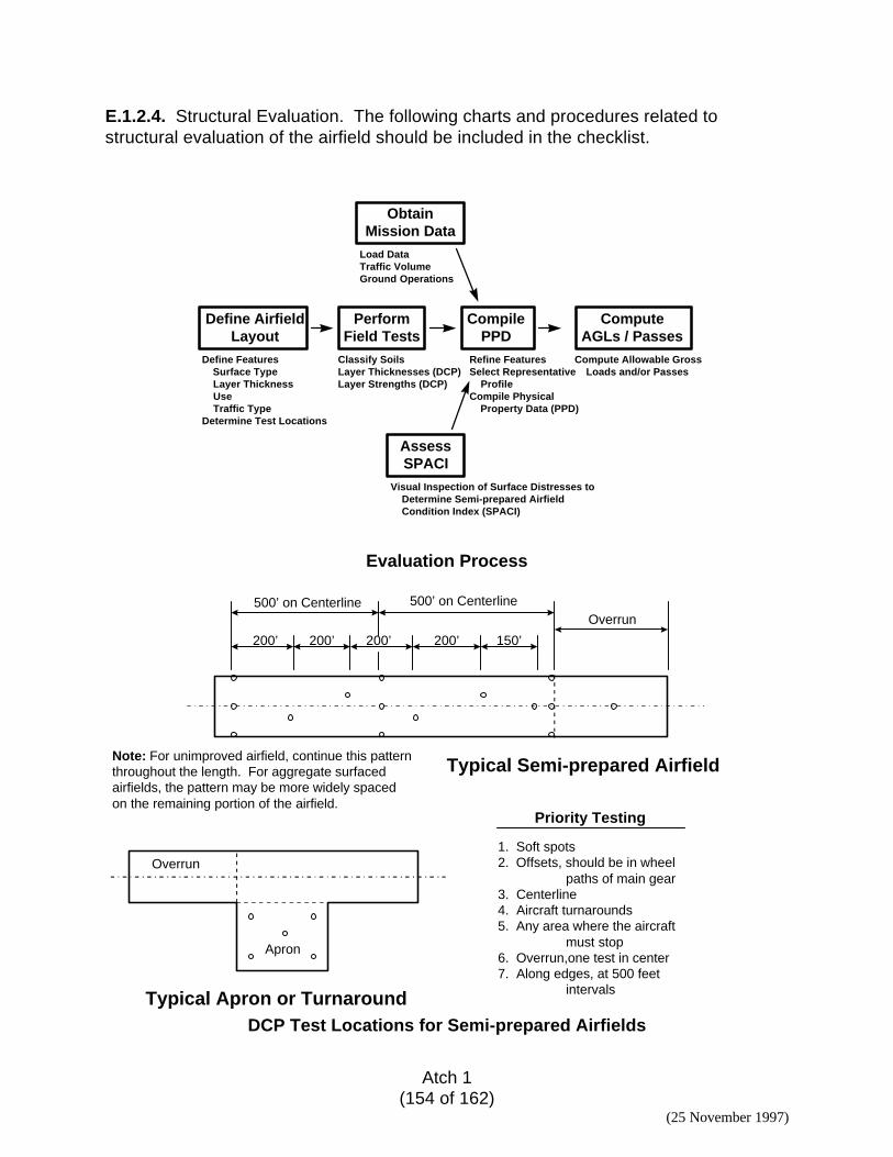
Atch 1(154 of 162)
(25 November 1997)
E.1.2.4. Structural Evaluation. The following charts and procedures related tostructural evaluation of the airfield should be included in the checklist.
ObtainMission Data
Define AirfieldLayout
PerformField Tests
CompilePPD
ComputeAGLs / Passes
AssessSPACI
Load DataTraffic VolumeGround Operations
Visual Inspection of Surface Distresses to Determine Semi-prepared Airfield Condition Index (SPACI)
Define Features Surface Type Layer Thickness Use Traffic TypeDetermine Test Locations
Classify SoilsLayer Thicknesses (DCP)Layer Strengths (DCP)
Compute Allowable Gross Loads and/or Passes
Refine FeaturesSelect Representative ProfileCompile Physical Property Data (PPD)
Evaluation Process
500’ on Centerline 500’ on CenterlineOverrun
200’200’ 200’200’ 150’
Note: For unimproved airfield, continue this patternthroughout the length. For aggregate surfacedairfields, the pattern may be more widely spacedon the remaining portion of the airfield.
Typical Semi-prepared Airfield
Priority Testing
1. Soft spots2. Offsets, should be in wheel
paths of main gear3. Centerline4. Aircraft turnarounds5. Any area where the aircraft
must stop6. Overrun,one test in center7. Along edges, at 500 feet
intervalsTypical Apron or Turnaround
Overrun
Apron
DCP Test Locations for Semi-prepared Airfields
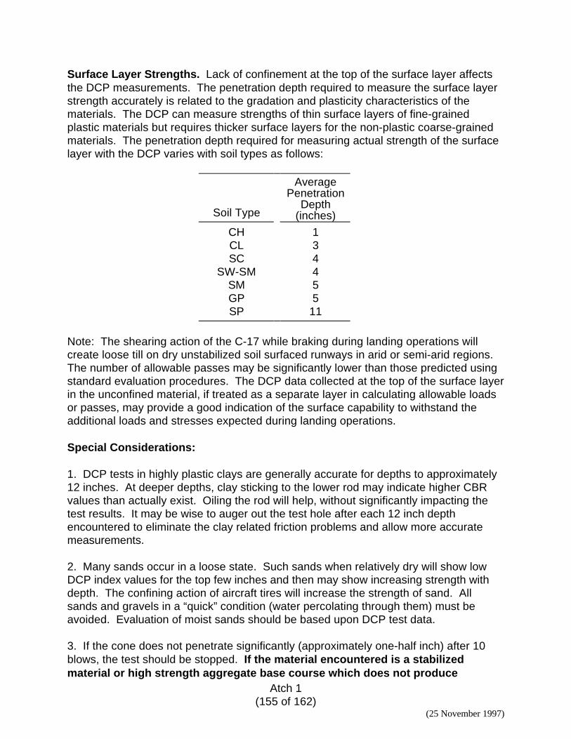
Atch 1(155 of 162)
(25 November 1997)
Surface Layer Strengths. Lack of confinement at the top of the surface layer affectsthe DCP measurements. The penetration depth required to measure the surface layerstrength accurately is related to the gradation and plasticity characteristics of thematerials. The DCP can measure strengths of thin surface layers of fine-grainedplastic materials but requires thicker surface layers for the non-plastic coarse-grainedmaterials. The penetration depth required for measuring actual strength of the surfacelayer with the DCP varies with soil types as follows:
Soil Type
AveragePenetration
Depth(inches)
CH 1CL 3SC 4
SW-SM 4SM 5GP 5SP 11
Note: The shearing action of the C-17 while braking during landing operations willcreate loose till on dry unstabilized soil surfaced runways in arid or semi-arid regions.The number of allowable passes may be significantly lower than those predicted usingstandard evaluation procedures. The DCP data collected at the top of the surface layerin the unconfined material, if treated as a separate layer in calculating allowable loadsor passes, may provide a good indication of the surface capability to withstand theadditional loads and stresses expected during landing operations.
Special Considerations:
1. DCP tests in highly plastic clays are generally accurate for depths to approximately12 inches. At deeper depths, clay sticking to the lower rod may indicate higher CBRvalues than actually exist. Oiling the rod will help, without significantly impacting thetest results. It may be wise to auger out the test hole after each 12 inch depthencountered to eliminate the clay related friction problems and allow more accuratemeasurements.
2. Many sands occur in a loose state. Such sands when relatively dry will show lowDCP index values for the top few inches and then may show increasing strength withdepth. The confining action of aircraft tires will increase the strength of sand. Allsands and gravels in a “quick” condition (water percolating through them) must beavoided. Evaluation of moist sands should be based upon DCP test data.
3. If the cone does not penetrate significantly (approximately one-half inch) after 10blows, the test should be stopped. If the material encountered is a stabilizedmaterial or high strength aggregate base course which does not produce
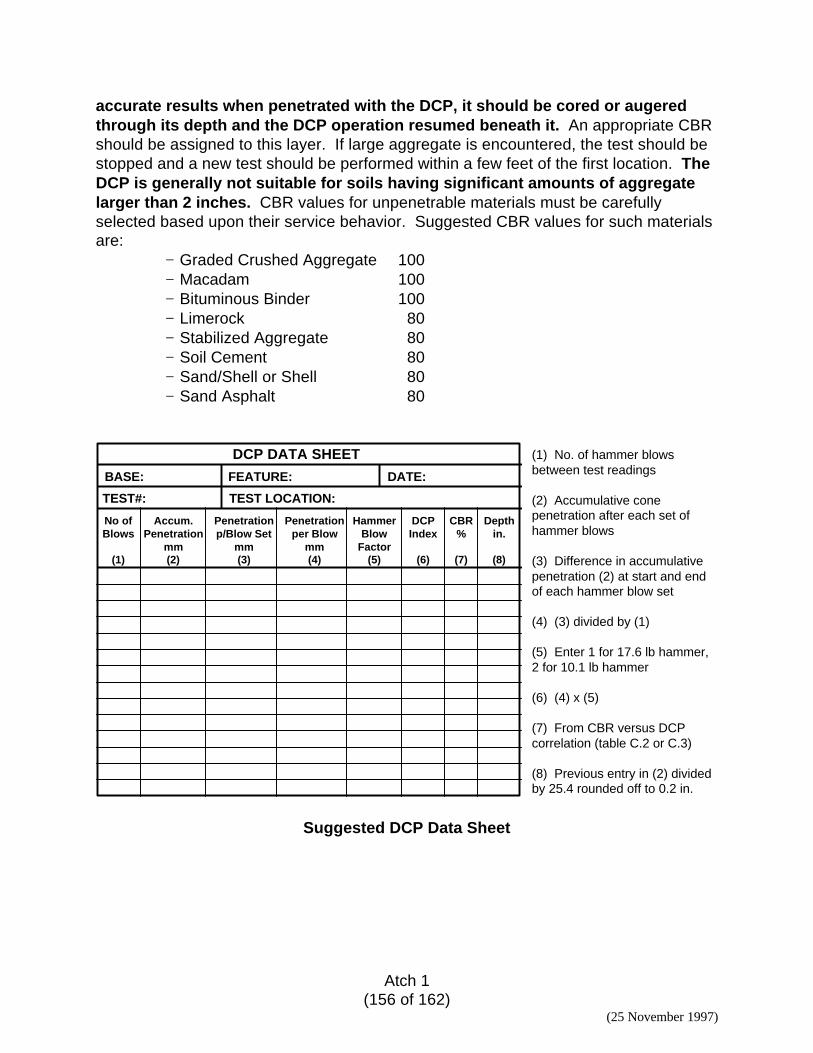
Atch 1(156 of 162)
(25 November 1997)
accurate results when penetrated with the DCP, it should be cored or augeredthrough its depth and the DCP operation resumed beneath it. An appropriate CBRshould be assigned to this layer. If large aggregate is encountered, the test should bestopped and a new test should be performed within a few feet of the first location. TheDCP is generally not suitable for soils having significant amounts of aggregatelarger than 2 inches. CBR values for unpenetrable materials must be carefullyselected based upon their service behavior. Suggested CBR values for such materialsare:
− Graded Crushed Aggregate 100− Macadam 100− Bituminous Binder 100− Limerock 80− Stabilized Aggregate 80− Soil Cement 80− Sand/Shell or Shell 80− Sand Asphalt 80
DCP DATA SHEET
No ofBlows
(1)
Accum.Penetration
mm(2)
Penetrationp/Blow Set
mm(3)
Penetrationper Blow
mm(4)
HammerBlow
Factor(5)
DCPIndex
(6)
CBR%
(7)
Depthin.
(8)
BASE: DATE:
TEST#:
FEATURE:
TEST LOCATION:
(1) No. of hammer blowsbetween test readings
(2) Accumulative cone penetration after each set ofhammer blows
(3) Difference in accumulativepenetration (2) at start and endof each hammer blow set
(4) (3) divided by (1)
(5) Enter 1 for 17.6 lb hammer,2 for 10.1 lb hammer
(6) (4) x (5)
(7) From CBR versus DCPcorrelation (table C.2 or C.3)
(8) Previous entry in (2) dividedby 25.4 rounded off to 0.2 in.
Suggested DCP Data Sheet
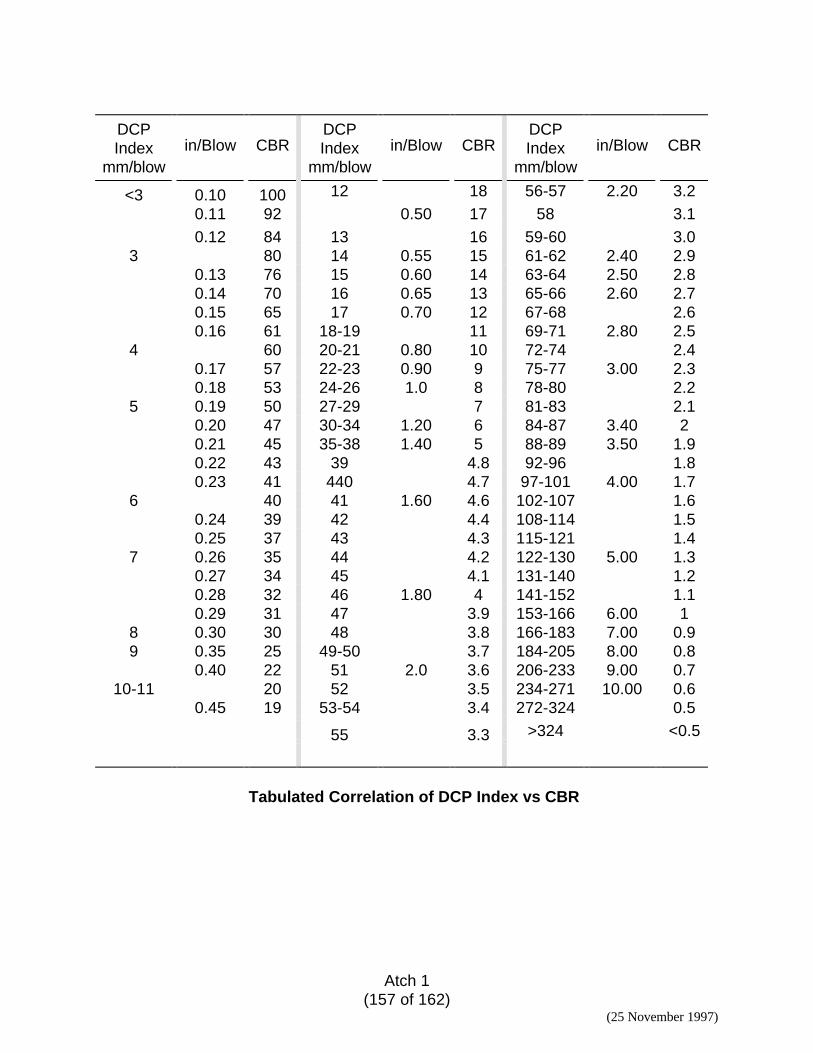
Atch 1(157 of 162)
(25 November 1997)
DCPIndex
mm/blowin/Blow CBR
DCPIndex
mm/blowin/Blow CBR
DCPIndex
mm/blowin/Blow CBR
<3 0.10 100 12 18 56-57 2.20 3.20.11 92 0.50 17 58 3.10.12 84 13 16 59-60 3.0
3 80 14 0.55 15 61-62 2.40 2.90.13 76 15 0.60 14 63-64 2.50 2.80.14 70 16 0.65 13 65-66 2.60 2.70.15 65 17 0.70 12 67-68 2.60.16 61 18-19 11 69-71 2.80 2.5
4 60 20-21 0.80 10 72-74 2.40.17 57 22-23 0.90 9 75-77 3.00 2.30.18 53 24-26 1.0 8 78-80 2.2
5 0.19 50 27-29 7 81-83 2.10.20 47 30-34 1.20 6 84-87 3.40 20.21 45 35-38 1.40 5 88-89 3.50 1.90.22 43 39 4.8 92-96 1.80.23 41 440 4.7 97-101 4.00 1.7
6 40 41 1.60 4.6 102-107 1.60.24 39 42 4.4 108-114 1.50.25 37 43 4.3 115-121 1.4
7 0.26 35 44 4.2 122-130 5.00 1.30.27 34 45 4.1 131-140 1.20.28 32 46 1.80 4 141-152 1.10.29 31 47 3.9 153-166 6.00 1
8 0.30 30 48 3.8 166-183 7.00 0.99 0.35 25 49-50 3.7 184-205 8.00 0.8
0.40 22 51 2.0 3.6 206-233 9.00 0.710-11 20 52 3.5 234-271 10.00 0.6
0.45 19 53-54 3.4 272-324 0.5
55 3.3 >324 <0.5
Tabulated Correlation of DCP Index vs CBR
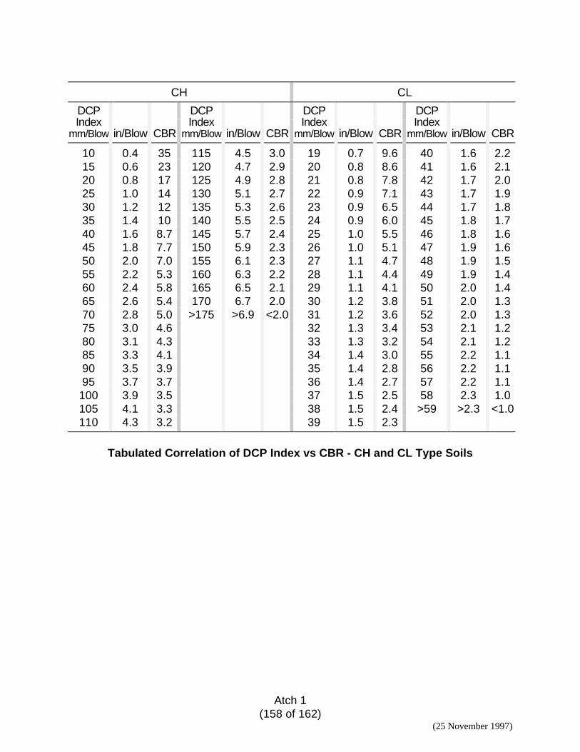
Atch 1(158 of 162)
(25 November 1997)
CH CL
DCPIndex
mm/Blow in/Blow CBR
DCPIndex
mm/Blow in/Blow CBR
DCPIndex
mm/Blow in/Blow CBR
DCPIndex
mm/Blow in/Blow CBR
10 0.4 35 115 4.5 3.0 19 0.7 9.6 40 1.6 2.215 0.6 23 120 4.7 2.9 20 0.8 8.6 41 1.6 2.120 0.8 17 125 4.9 2.8 21 0.8 7.8 42 1.7 2.025 1.0 14 130 5.1 2.7 22 0.9 7.1 43 1.7 1.930 1.2 12 135 5.3 2.6 23 0.9 6.5 44 1.7 1.835 1.4 10 140 5.5 2.5 24 0.9 6.0 45 1.8 1.740 1.6 8.7 145 5.7 2.4 25 1.0 5.5 46 1.8 1.645 1.8 7.7 150 5.9 2.3 26 1.0 5.1 47 1.9 1.650 2.0 7.0 155 6.1 2.3 27 1.1 4.7 48 1.9 1.555 2.2 5.3 160 6.3 2.2 28 1.1 4.4 49 1.9 1.460 2.4 5.8 165 6.5 2.1 29 1.1 4.1 50 2.0 1.465 2.6 5.4 170 6.7 2.0 30 1.2 3.8 51 2.0 1.370 2.8 5.0 >175 >6.9 <2.0 31 1.2 3.6 52 2.0 1.375 3.0 4.6 32 1.3 3.4 53 2.1 1.280 3.1 4.3 33 1.3 3.2 54 2.1 1.285 3.3 4.1 34 1.4 3.0 55 2.2 1.190 3.5 3.9 35 1.4 2.8 56 2.2 1.195 3.7 3.7 36 1.4 2.7 57 2.2 1.1
100 3.9 3.5 37 1.5 2.5 58 2.3 1.0105 4.1 3.3 38 1.5 2.4 >59 >2.3 <1.0110 4.3 3.2 39 1.5 2.3
Tabulated Correlation of DCP Index vs CBR - CH and CL Type Soils

Atch 1(159 of 162)
(25 November 1997)
SUMMARY OF PHYSICAL PROPERTY DATA: SEMI-PREPARED AIRFIELDSFACILITY SURFACE SUBBASE SUBGRADE
FEAT IDENT LGTH(ft)
WDTH(ft)
COND THCK (in)
DESCRP CBR THCK (in)
DESCRP CBR THCK (in)
DESCRP CBR
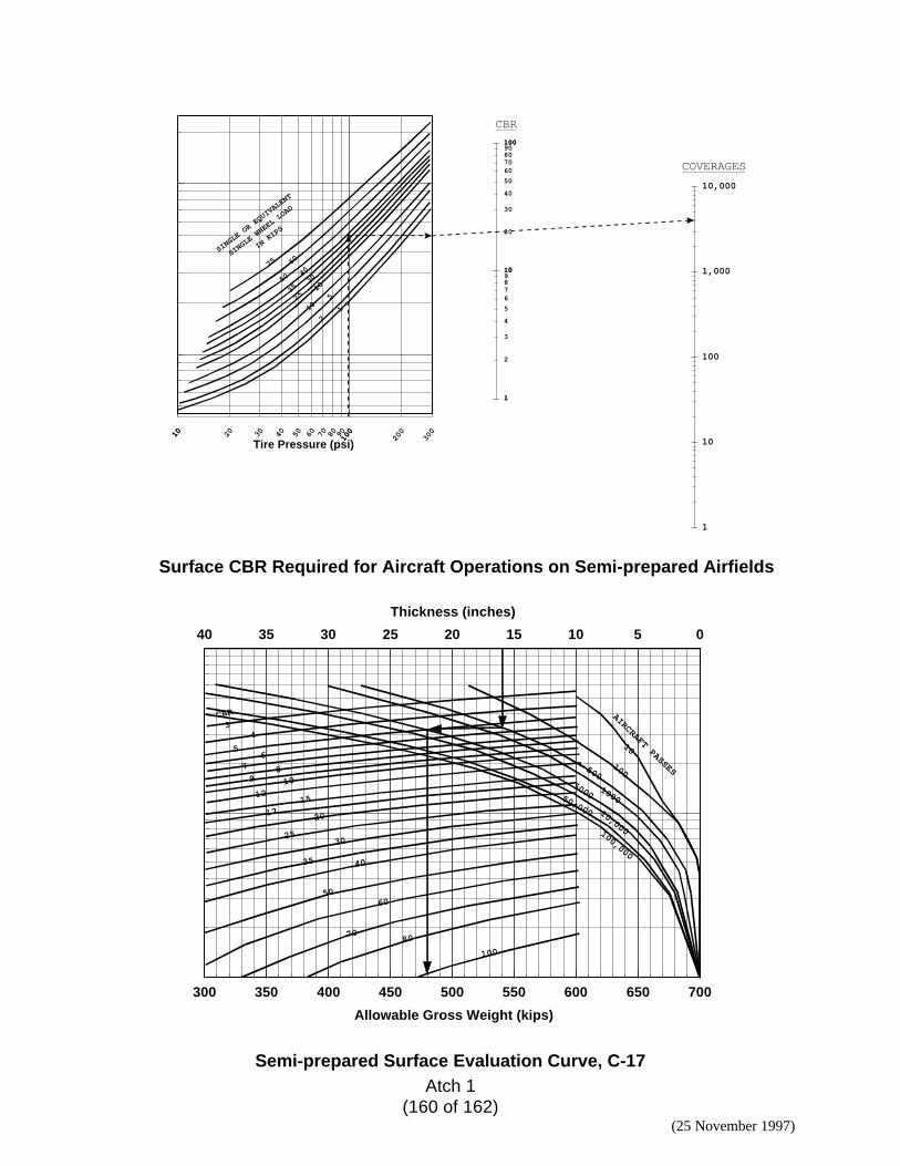
Atch 1(160 of 162)
(25 November 1997)
10 20 30 40 50 60 70 80 90100
200
30010 100
Tire Pressure (psi)
75 60
5040
35
30
2520
10
52
1
SINGLE OR EQUIVALENT
SINGLE WHEEL LOAD
IN KIPS
1
2
3
4
5
678910
20
30
40
50
60708090100
1
10
100
1
10
100
1,000
10,000
CBR
COVERAGES
Surface CBR Required for Aircraft Operations on Semi-prepared Airfields
300 350 400 450 500 550 600 650 700
Allowable Gross Weight (kips)
0510152025303540
Thickness (inches)
AIRCRAFT PASSES100
10,000
50,000
50001000
100,000
500
CBR
34
56
7 89 10
1215
17 20
2530
35 40
5060
7080
100
10
Semi-prepared Surface Evaluation Curve, C-17
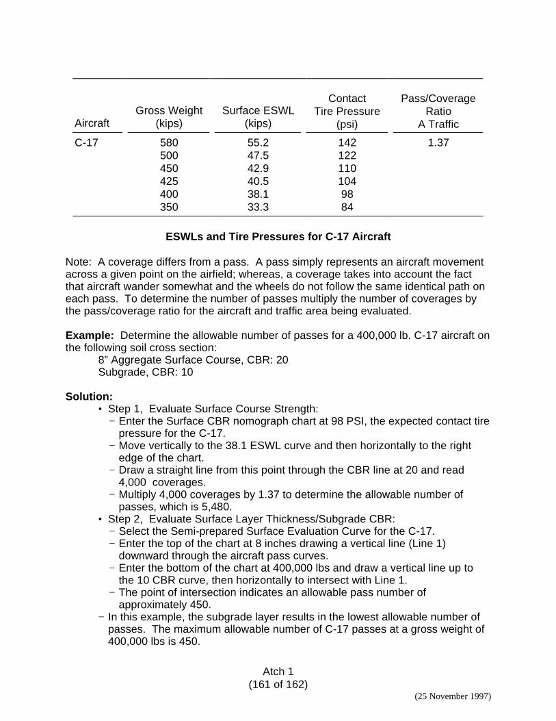
Atch 1(161 of 162)
(25 November 1997)
AircraftGross Weight
(kips)Surface ESWL
(kips)
ContactTire Pressure
(psi)
Pass/CoverageRatio
A Traffic
C-17 580 55.2 142 1.37500 47.5 122450 42.9 110425 40.5 104400 38.1 98350 33.3 84
ESWLs and Tire Pressures for C-17 Aircraft
Note: A coverage differs from a pass. A pass simply represents an aircraft movementacross a given point on the airfield; whereas, a coverage takes into account the factthat aircraft wander somewhat and the wheels do not follow the same identical path oneach pass. To determine the number of passes multiply the number of coverages bythe pass/coverage ratio for the aircraft and traffic area being evaluated.
Example: Determine the allowable number of passes for a 400,000 lb. C-17 aircraft onthe following soil cross section:
8” Aggregate Surface Course, CBR: 20Subgrade, CBR: 10
Solution:• Step 1, Evaluate Surface Course Strength:
− Enter the Surface CBR nomograph chart at 98 PSI, the expected contact tirepressure for the C-17.
− Move vertically to the 38.1 ESWL curve and then horizontally to the rightedge of the chart.
− Draw a straight line from this point through the CBR line at 20 and read4,000 coverages.
− Multiply 4,000 coverages by 1.37 to determine the allowable number ofpasses, which is 5,480.
• Step 2, Evaluate Surface Layer Thickness/Subgrade CBR:− Select the Semi-prepared Surface Evaluation Curve for the C-17.− Enter the top of the chart at 8 inches drawing a vertical line (Line 1)
downward through the aircraft pass curves.− Enter the bottom of the chart at 400,000 lbs and draw a vertical line up to
the 10 CBR curve, then horizontally to intersect with Line 1.− The point of intersection indicates an allowable pass number of
approximately 450.− In this example, the subgrade layer results in the lowest allowable number of
passes. The maximum allowable number of C-17 passes at a gross weight of400,000 lbs is 450.
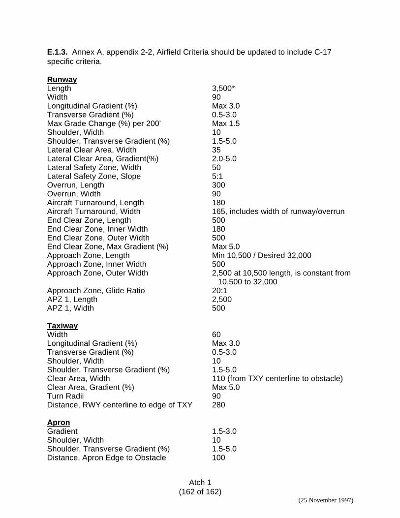
Atch 1(162 of 162)
(25 November 1997)
E.1.3. Annex A, appendix 2-2, Airfield Criteria should be updated to include C-17specific criteria.
RunwayLength 3,500*Width 90Longitudinal Gradient (%) Max 3.0Transverse Gradient (%) 0.5-3.0Max Grade Change (%) per 200' Max 1.5Shoulder, Width 10Shoulder, Transverse Gradient (%) 1.5-5.0Lateral Clear Area, Width 35Lateral Clear Area, Gradient(%) 2.0-5.0Lateral Safety Zone, Width 50Lateral Safety Zone, Slope 5:1Overrun, Length 300Overrun, Width 90Aircraft Turnaround, Length 180Aircraft Turnaround, Width 165, includes width of runway/overrunEnd Clear Zone, Length 500End Clear Zone, Inner Width 180End Clear Zone, Outer Width 500End Clear Zone, Max Gradient (%) Max 5.0Approach Zone, Length Min 10,500 / Desired 32,000Approach Zone, Inner Width 500Approach Zone, Outer Width 2,500 at 10,500 length, is constant from
10,500 to 32,000Approach Zone, Glide Ratio 20:1APZ 1, Length 2,500APZ 1, Width 500
TaxiwayWidth 60Longitudinal Gradient (%) Max 3.0Transverse Gradient (%) 0.5-3.0Shoulder, Width 10Shoulder, Transverse Gradient (%) 1.5-5.0Clear Area, Width 110 (from TXY centerline to obstacle)Clear Area, Gradient (%) Max 5.0Turn Radii 90Distance, RWY centerline to edge of TXY 280
ApronGradient 1.5-3.0Shoulder, Width 10Shoulder, Transverse Gradient (%) 1.5-5.0Distance, Apron Edge to Obstacle 100
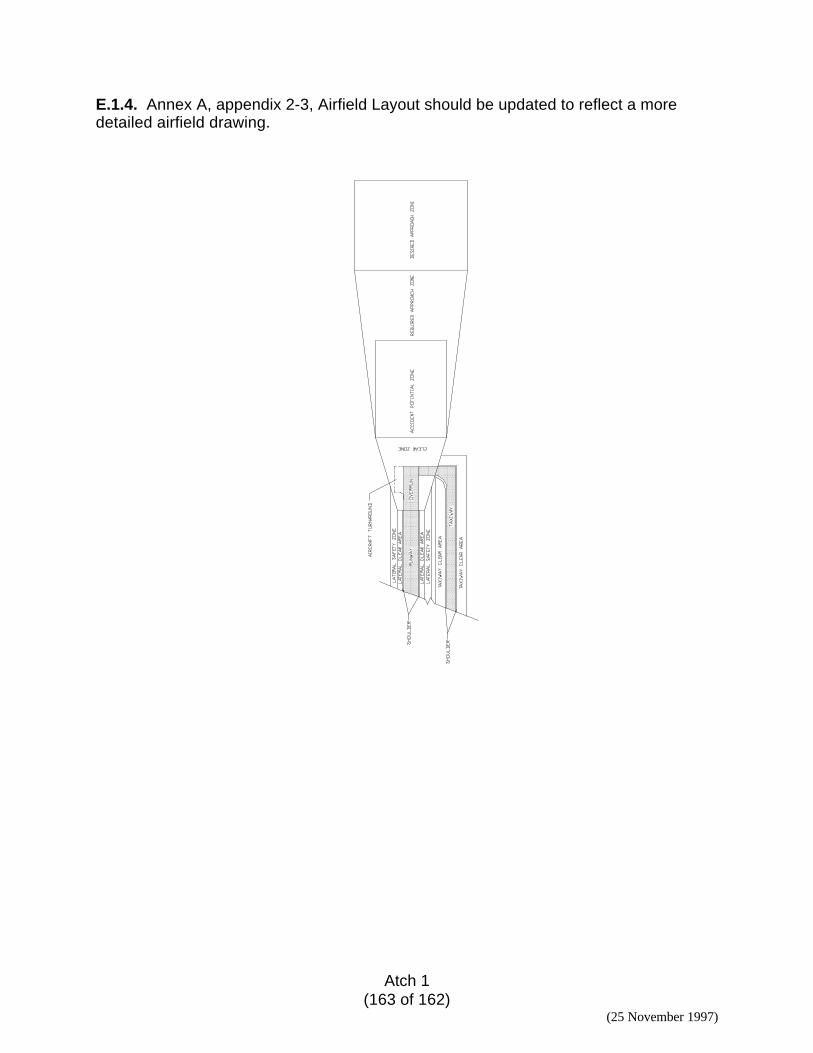
Atch 1(163 of 162)
(25 November 1997)
E.1.4. Annex A, appendix 2-3, Airfield Layout should be updated to reflect a moredetailed airfield drawing.