Embed Size (px)
DESCRIPTION
FRM - Bionic Turtle T3 - Products
Citation preview
T3. Markets & Products FRM 2011 Study Notes – Vol. III
By David Harper, CFA FRM CIPM
www.bionicturtle.com
FRM 2011 MARKETS & PRODUCTS 1 www.bionicturtle.com
Table of Contents
Hull, Chapter 1, Introduction 2
Hull, Chapter 2: Mechanics of Futures Markets 10
Hull, Chapter 3: Hedging Strategies Using Futures 21
Hull, Chapter 4: Interest Rates 30
Hull, Chapter 5: Determination of Forward and Futures Prices 40
Hull, Chapter 6: Interest Rate Futures 56
Hull, Chapter 7: Swaps 72
Hull, Chapter 9: Properties of Stock Options 86
Hull, Chapter 10: Trading Strategies Involving Options 93
McDonald, Chapter 6: Commodity Forwards and Futures 101
Geman, Chapter 1: Fundamentals of Commodity Spot and Futures Markets: Instruments,
Exchanges and Strategies 115
Cornett, Chapter 14: Foreign Exchange Risk 123
Cornett, Appendix 15A: Mechanisms for Dealing with Sovereign Risk Exposure 129
Fabozzi, Chapter 13: Corporate Bonds 132
FRM 2011 MARKETS & PRODUCTS 2 www.bionicturtle.com
Hull, Chapter 1,
Introduction
In this chapter…
Differentiate between an open outcry system and electronic trading. Describe the over‐the‐counter market and how it differs from trading on an
exchange, including advantages and disadvantages. Differentiate between options, forwards, and futures contracts. Calculate and identify option and forward contract payoffs. Describe, contrast, & calculate the payoffs from hedging strategies (and from
speculative strategies) involving forward contracts and options. Calculate an arbitrage payoff and describe how arbitrage opportunities are
ephemeral. Describe some of the risks that can arise from the (mis)use of derivatives. Define:
Derivative Market maker Spot contract, Forward contract, and Futures contract Call option and Put option American option and European option Long position and short position Exercise (strike) price Expiration (maturity) date Bid price and offer price Bid‐offer spread Hedgers and speculators Arbitrageurs
Differentiate between an open outcry system and electronic trading
Open outcry
Traders physically meet on exchange floor, shouting, using hand signals
Electronic trading
Electronic matching of trades
FRM 2011 MARKETS & PRODUCTS 3 www.bionicturtle.com
Describe the over the counter market and how it differs from trading on
an exchange, including advantages and disadvantages
Over-the-counter (OTC)
Network of dealers linked by recorded phone conversations and computers
Trades between two counterparties
Advantage
Non-standard terms: participants can negotiate terms
Disadvantage
Some credit (counterparty) risk
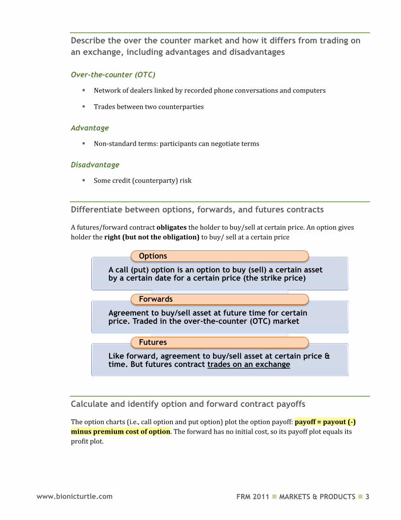
Differentiate between options, forwards, and futures contracts
A futures/forward contract obligates the holder to buy/sell at certain price. An option gives
holder the right (but not the obligation) to buy/ sell at a certain price
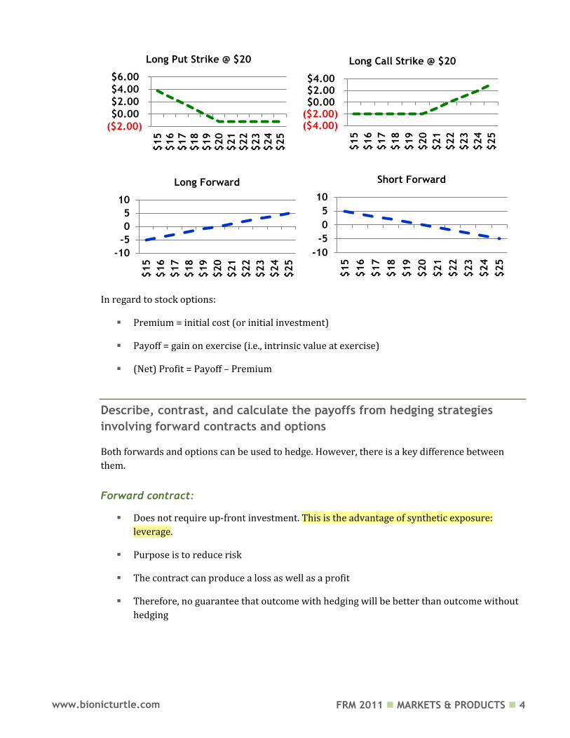
Calculate and identify option and forward contract payoffs
The option charts (i.e., call option and put option) plot the option payoff: payoff = payout (-)
minus premium cost of option. The forward has no initial cost, so its payoff plot equals its
profit plot.
A call (put) option is an option to buy (sell) a certain asset by a certain date for a certain price (the strike price)
Options
Agreement to buy/sell asset at future time for certain price. Traded in the over-the-counter (OTC) market
Forwards
Like forward, agreement to buy/sell asset at certain price & time. But futures contract trades on an exchange
Futures
FRM 2011 MARKETS & PRODUCTS 4 www.bionicturtle.com
In regard to stock options:
Premium = initial cost (or initial investment)
Payoff = gain on exercise (i.e., intrinsic value at exercise)
(Net) Profit = Payoff – Premium
Describe, contrast, and calculate the payoffs from hedging strategies
involving forward contracts and options
Both forwards and options can be used to hedge. However, there is a key difference between
them.
Forward contract:
Does not require up-front investment. This is the advantage of synthetic exposure:
leverage.
Purpose is to reduce risk
The contract can produce a loss as well as a profit
Therefore, no guarantee that outcome with hedging will be better than outcome without
hedging
($2.00)
$0.00
$2.00
$4.00
$6.00
$15
$16
$17
$18
$19
$20
$21
$22
$23
$24
$25
Long Put Strike @ $20
($4.00)($2.00)$0.00$2.00$4.00
$15
$16
$17
$18
$19
$20
$21
$22
$23
$24
$25
Long Call Strike @ $20
-10
-5
0
5
10
$15
$16
$17
$18
$19
$20
$21
$22
$23
$24
$25
Long Forward
-10
-5
0
5
10
$15
$16
$17
$18
$19
$20
$21
$22
$23
$24
$25
Short Forward
FRM 2011 MARKETS & PRODUCTS 5 www.bionicturtle.com
Option:
Requires up-front premium
Asymmetric
Provides insurance
Unlike the forward contract, limits downside. This is the essential difference between a
forward hedge and an option hedge (e.g., buying a put option): the forward does not have
a premium, while the option requires a premium. But the option is asymmetric: it does
not need to be exercised, so the gain can be preserved.
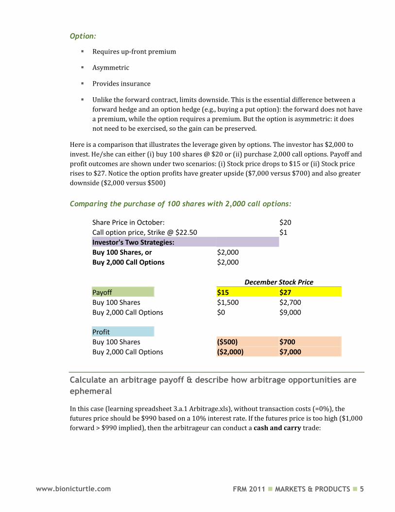
Here is a comparison that illustrates the leverage given by options. The investor has $2,000 to
invest. He/she can either (i) buy 100 shares @ $20 or (ii) purchase 2,000 call options. Payoff and
profit outcomes are shown under two scenarios: (i) Stock price drops to $15 or (ii) Stock price
rises to $27. Notice the option profits have greater upside ($7,000 versus $700) and also greater
downside ($2,000 versus $500)
Comparing the purchase of 100 shares with 2,000 call options:
Share Price in October: $20
Call option price, Strike @ $22.50 $1
Investor's Two Strategies:
Buy 100 Shares, or $2,000
Buy 2,000 Call Options $2,000
December Stock Price
Payoff
$15 $27
Buy 100 Shares $1,500 $2,700
Buy 2,000 Call Options $0 $9,000
Profit
Buy 100 Shares ($500) $700
Buy 2,000 Call Options ($2,000) $7,000
Calculate an arbitrage payoff & describe how arbitrage opportunities are
ephemeral
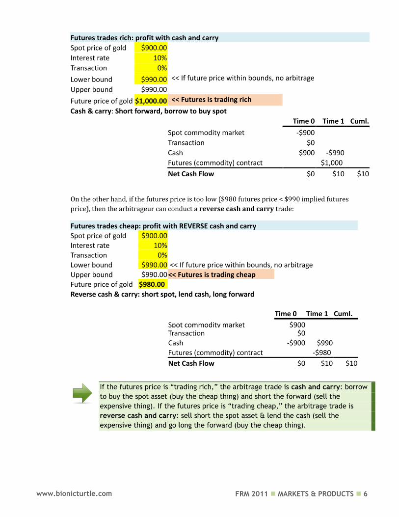
In this case (learning spreadsheet 3.a.1 Arbitrage.xls), without transaction costs (=0%), the
futures price should be $990 based on a 10% interest rate. If the futures price is too high ($1,000
forward > $990 implied), then the arbitrageur can conduct a cash and carry trade:
FRM 2011 MARKETS & PRODUCTS 6 www.bionicturtle.com
Futures trades rich: profit with cash and carry
Spot price of gold $900.00 Interest rate 10% Transaction 0% Lower bound $990.00 << If future price within bounds, no arbitrage
Upper bound $990.00 Future price of gold $1,000.00 << Futures is trading rich
Cash & carry: Short forward, borrow to buy spot
Time 0 Time 1 Cuml.
Spot commodity market -$900
Transaction $0
Cash $900 -$990
Futures (commodity) contract
$1,000
Net Cash Flow $0 $10 $10
On the other hand, if the futures price is too low ($980 futures price < $990 implied futures
price), then the arbitrageur can conduct a reverse cash and carry trade:
Futures trades cheap: profit with REVERSE cash and carry Spot price of gold $900.00
Interest rate 10%
Transaction 0%
Lower bound $990.00 << If future price within bounds, no arbitrage Upper bound $990.00 << Futures is trading cheap
Future price of gold $980.00
Reverse cash & carry: short spot, lend cash, long forward
2
reverse cash & carry
Time 0 Time 1 Cuml.
Spot commodity market $900
Transaction $0
Cash -$900 $990
Futures (commodity) contract
-$980
Net Cash Flow $0 $10 $10
If the futures price is “trading rich,” the arbitrage trade is cash and carry: borrow
to buy the spot asset (buy the cheap thing) and short the forward (sell the
expensive thing). If the futures price is “trading cheap,” the arbitrage trade is
reverse cash and carry: sell short the spot asset & lend the cash (sell the
expensive thing) and go long the forward (buy the cheap thing).
FRM 2011 MARKETS & PRODUCTS 7 www.bionicturtle.com
Describe some of the risks that can arise from the (mis)use of derivatives
There are three primary derivative uses:
Hedging
Speculation
Arbitrage
The key risk (danger) is that traders with mandates to hedge (or arbitrage) become speculators.
Other Derivative Mishaps and What We Can Learn (Unassigned Hull, Chapter 34):
Risk must be quantified and risk limits defined
Exceeding risk limits not acceptable even when profits result
Do not assume that a trader with a good track record will always be right
Be diversified
Scenario analysis and stress testing is important
Lessons for Financial Institutions (Unassigned Hull, Chapter 34):
Do not give too much independence to star traders
Separate the front middle and back office
Models can be wrong
Be conservative in recognizing inception profits
Do not sell clients inappropriate products
Liquidity risk is very important
There are dangers when many are following the same strategy
Do not finance long-term assets with short-term liabilities
Market transparency is important
Lessons for non-Financial Institutions (Unassigned Hull, Chapter 34)
It is important to fully understand the products you trade
Beware of hedgers becoming speculators
It can be dangerous to make the Treasurer’s department a profit center

FRM 2011 MARKETS & PRODUCTS 8 www.bionicturtle.com
Define…
… Derivative
A financial instrument whose value depends on (or derives from) the values of other, more basic,
underlying variables
Underlying can be price of traded asset, or
Anything!
… Market Maker
A trader who is willing to quote both bid and offer prices for an asset.
… Spot contract, Forward contract, and Futures contract
Spot contract: price for immediate delivery
Forward contract: price for future delivery
Futures contract: price for future delivery
… Call option and Put option
Call option: Option (right but not the obligation) to buy asset by date for [strike] price
Put option: Option (right but not obligation) to sell asset by date for [strike] price
… American option and European option
American option: Can be exercised at prior to expiration, perhaps at any time during its
life (if vesting restrictions do not prohibit)
European option: Can be exercised only at maturity
FRM 2011 MARKETS & PRODUCTS 9 www.bionicturtle.com
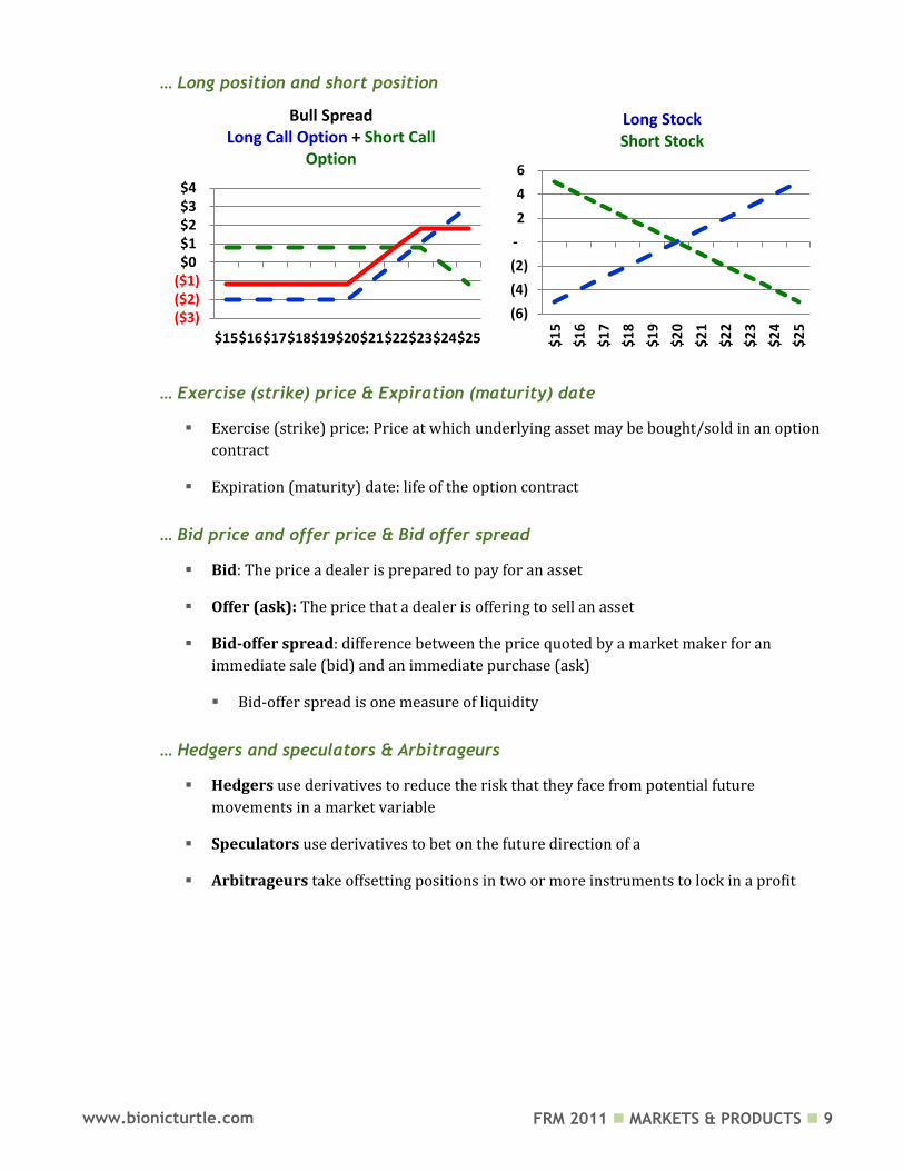
… Long position and short position
… Exercise (strike) price & Expiration (maturity) date
Exercise (strike) price: Price at which underlying asset may be bought/sold in an option
contract
Expiration (maturity) date: life of the option contract
… Bid price and offer price & Bid offer spread
Bid: The price a dealer is prepared to pay for an asset
Offer (ask): The price that a dealer is offering to sell an asset
Bid-offer spread: difference between the price quoted by a market maker for an
immediate sale (bid) and an immediate purchase (ask)
Bid-offer spread is one measure of liquidity
… Hedgers and speculators & Arbitrageurs
Hedgers use derivatives to reduce the risk that they face from potential future
movements in a market variable
Speculators use derivatives to bet on the future direction of a
Arbitrageurs take offsetting positions in two or more instruments to lock in a profit
($3)($2)($1)$0$1$2$3$4
$15$16$17$18$19$20$21$22$23$24$25
Bull Spread Long Call Option + Short Call
Option
(6)
(4)
(2)
-
2
4
6
$1
5
$1
6
$1
7
$1
8
$1
9
$2
0
$2
1
$2
2
$2
3
$2
4
$2
5
Long Stock Short Stock
FRM 2011 MARKETS & PRODUCTS 10 www.bionicturtle.com
Hull, Chapter 2:
Mechanics of
Futures Markets
In this chapter…
Define and describe the key features of a futures contract. Compare and contrast forward and futures contracts. Explain the convergence of futures and spot prices. Describe the rationale for margin requirements and explain how they work. Describe the role of a clearinghouse in futures transactions. Describe the role of collateralization in the over‐the‐counter market and
compare it to the margining system. Identify and describe the differences between a normal and inverted futures
market. Describe the mechanics of the delivery process and contrast it with cash
settlement. Define and demonstrate an understanding of the impact of different order
types, including: market, limit, stop‐loss, stop‐limit, market‐if‐touched, discretionary, time‐of‐day, open, and fill‐or‐kill
Define: Notice of intention to deliver Limit up and limit down Margin account Initial margin, maintenance margin, variation margin and clearing margin Collateralization Settlement price Open interest
Define and describe the key features of a futures contract
A futures contract is a standardized contract that trades on a futures exchange to buy or sell
an underlying asset at a delivery date at a pre-set futures price. The specifications of a futures
contract include, but are not limited to:
Asset
Contract Size
Delivery Arrangement
FRM 2011 MARKETS & PRODUCTS 11 www.bionicturtle.com
Delivery Months
Price Quotes
Price limits and position limits
For example, consider the underlying asset in the case of a Treasury bond/note:
A Treasury bond futures contract is made on the underlying U.S. Treasury with maturity
of at least 15 years and not callable within 15 years (15 years ≤ T bond).
A Treasury note futures contract is made on the underlying U.S. Treasury with maturity
of at least 6.5 years but not greater than 10 years (6.5 ≤ T note ≤ 10 years).
When the asset is a commodity (e.g., cotton, orange juice), the exchange specifies a
grade (quality).
Contract Size
Contract size varies by the type of futures contract:
Treasury bond futures: contract size is a face value of $100,000
S&P 500 futures contract is index $250 (multiplier of 250X)
NASDAQ futures contract is index $100 (multiplier of 100X)
Recently, “mini contracts” have been introduced: These have multipliers of 50X
for the S&P and 20X for the NASDAQ. In other words, each contract is one-fifth the
price in order to attract smaller investors.
A common test question involves S&P 500 Index futures contract. Please note
the multiple for the S&P 500 contract is $250; e.g., if the index value is 1400,
then one contract is worth $350,00
Delivery Arrangement
The exchange specifies delivery location. The exchange must specify the delivery month; this can
be the entire month or a sub-period of the month.
Delivery Months
The exchange must specify the precise period during the month when delivery can be made. For
many futures contracts, the delivery period is the whole month.
Price Quotes
The exchange defines how prices are quoted; e.g., crude oil is quoted in dollars and cents
FRM 2011 MARKETS & PRODUCTS 12 www.bionicturtle.com
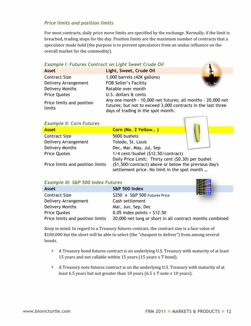
Price limits and position limits
For most contracts, daily price move limits are specified by the exchange. Normally, if the limit is
breached, trading stops for the day. Position limits are the maximum number of contracts that a
speculator made hold (the purpose is to prevent speculators from an undue influence on the
overall market for the commodity).
Example I: Futures Contract on Light Sweet Crude Oil
Asset Light, Sweet, Crude Oil
Contract Size 1,000 barrels (42K gallons)
Delivery Arrangement FOB Seller’s Facility
Delivery Months Ratable over month
Price Quotes U.S. dollars & cents
Price limits and position limits
Any one month - 10,000 net futures; all months - 20,000 net futures; but not to exceed 3,000 contracts in the last three days of trading in the spot month.
Example II: Corn Futures
Asset Corn (No. 2 Yellow.. )
Contract Size 5000 bushels
Delivery Arrangement Toledo, St. Louis
Delivery Months Dec, Mar, May, Jul, Sep
Price Quotes 1/4 cent/bushel ($12.50/contract)
Price limits and position limits Daily Price Limit: Thirty cent ($0.30) per bushel ($1,500/contract) above or below the previous day's settlement price. No limit in the spot month …
Example III: S&P 500 Index Futures
Asset S&P 500 Index
Contract Size $250 x S&P 500 Futures Price
Delivery Arrangement Cash settlement
Delivery Months Mar, Jun, Sep, Dec
Price Quotes 0.05 index points = $12.50
Price limits and position limits 20,000 net long or short in all contract months combined
Keep in mind: In regard to a Treasury futures contract, the contract size is a face value of
$100,000 but the short will be able to select (the “cheapest to deliver”) from among several
bonds.
A Treasury bond futures contract is on underlying U.S. Treasury with maturity of at least
15 years and not callable within 15 years (15 years ≤ T bond).
A Treasury note futures contract is on the underlying U.S. Treasury with maturity of at
least 6.5 years but not greater than 10 years (6.5 ≤ T note ≤ 10 years).
FRM 2011 MARKETS & PRODUCTS 13 www.bionicturtle.com
Mini contracts
S&P 500 futures contract is index $250 (multiplier of 250X)
S&P 500 “mini” = $50 x S&P Index
NASDAQ futures contract is index $100 (multiplier of 100X)
NASDAQ “mini” = $20 x NASDQ (each contract is one-fifth the price, to attract smaller
investors)
Futures Positions: Distinguish between a long futures position and a short futures position and
explain how futures positions are settled
A long-futures position agrees to buy in the future and a short-futures position agrees to sell in
the future. The price mechanism maintains a balance between buyers and sellers. For example, if
there are more buyers than sellers, the price increases until new sellers enter the futures market.
Most futures contracts do not lead to delivery, because most trades “close out” their positions
before delivery. Closing out a position means entering into the opposite type of trade from the
original.
Exchanges and Regulation
Chicago Board of Trade (CBOT, www.cbot.com)
Chicago Mercantile Exchange (CME, www.cme.com)
London International Financial Futures and Options Exchange (www.liffe.com)
Eurex (www.eurexchange.com)
Regulation: Commodity Futures Trading Commission (CFTC, www.cftc.gov)
Operations of Margins: (i) Describe the marking to market procedure, the initial margin, and the
maintenance margin (ii) Compute the variation margin
When an investor enters into a futures contract, the broker requires an initial margin deposit
into the margin account. At the end of each trading day, the margin account is marked-to-market.
If the account balance falls below the maintenance margin (i.e., typically lower than the initial
margin), a margin call requires the investors to “top up” the account back to the initial margin
amount.
Margin account: Broker requires deposit.
Initial margin: Must be deposited when contract is initiated.
Mark-to-market: At the end of each trading day, margin account is adjusted to reflect
gains or losses.
FRM 2011 MARKETS & PRODUCTS 14 www.bionicturtle.com
Maintenance margin: Investor can withdraw funds in the margin account in excess of
the initial margin. A maintenance margin guarantees that the balance in the margin
account never gets negative (the maintenance margin is lower than the initial margin).
Margin call: When the balance in the margin account falls below the maintenance
margin, broker executes a margin call. The next day, the investor needs to “top up” the
margin account back to the initial margin level.
Variation margin: Extra funds deposited by the investor after receiving a margin call.
There is only a variation margin if and when there is a margin call.
Variation margin = initial margin – margin account balance
The maintenance margin is a trigger level—once triggered, the investor must
―top up‖ to the initial margin, which is greater than the maintenance level.
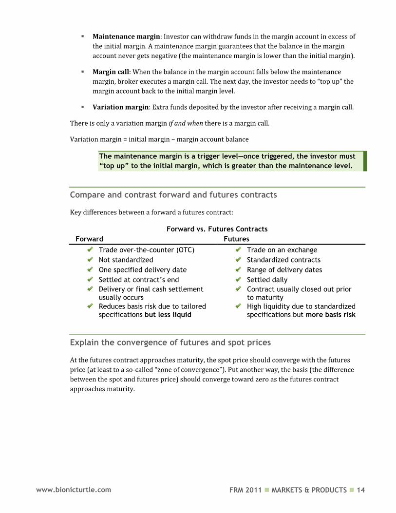
Compare and contrast forward and futures contracts
Key differences between a forward a futures contract:
Forward vs. Futures Contracts
Forward Futures
Trade over-the-counter (OTC) Trade on an exchange
Not standardized Standardized contracts
One specified delivery date Range of delivery dates
Settled at contract’s end Settled daily
Delivery or final cash settlement usually occurs
Contract usually closed out prior to maturity
Reduces basis risk due to tailored specifications but less liquid
High liquidity due to standardized specifications but more basis risk
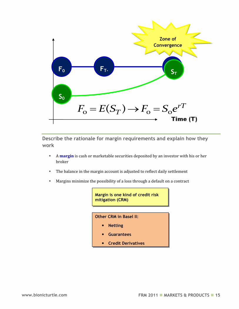
Explain the convergence of futures and spot prices
At the futures contract approaches maturity, the spot price should converge with the futures
price (at least to a so-called “zone of convergence”). Put another way, the basis (the difference
between the spot and futures price) should converge toward zero as the futures contract
approaches maturity.
FRM 2011 MARKETS & PRODUCTS 15 www.bionicturtle.com
Describe the rationale for margin requirements and explain how they
work
A margin is cash or marketable securities deposited by an investor with his or her
broker
The balance in the margin account is adjusted to reflect daily settlement
Margins minimize the possibility of a loss through a default on a contract
F0
S0
ST FT-
1
0 0 0( ) rTTF E S F S e
Zone of
Convergence
Margin is one kind of credit risk mitigation (CRM)
Other CRM in Basel II:
Netting
Guarantees
Credit Derivatives
FRM 2011 MARKETS & PRODUCTS 16 www.bionicturtle.com
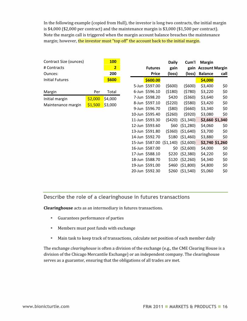
In the following example (copied from Hull), the investor is long two contracts, the initial margin
is $4,000 ($2,000 per contract) and the maintenance margin is $3,000 ($1,500 per contract).
Note the margin call is triggered when the margin account balance breaches the maintenance
margin; however, the investor must “top off” the account back to the initial margin.
Describe the role of a clearinghouse in futures transactions
Clearinghouse acts as an intermediary in futures transactions.
Guarantees performance of parties
Members must post funds with exchange
Main task to keep track of transactions, calculate net position of each member daily
The exchange clearinghouse is often a division of the exchange (e.g., the CME Clearing House is a
division of the Chicago Mercantile Exchange) or an independent company. The clearinghouse
serves as a guarantor, ensuring that the obligations of all trades are met.
Contract Size (ounces) 100
# Contracts 2
Ounces: 200
Initial Futures $600
Margin Per Total
Initial margin $2,000 $4,000
Maintenance margin $1,500 $3,000
Daily Cum'l Margin
Futures gain gain Account Margin
Price (loss) (loss) Balance call
$600.00
$4,000
5-Jun $597.00 ($600) ($600) $3,400 $0
6-Jun $596.10 ($180) ($780) $3,220 $0
7-Jun $598.20 $420 ($360) $3,640 $0
8-Jun $597.10 ($220) ($580) $3,420 $0
9-Jun $596.70 ($80) ($660) $3,340 $0
10-Jun $595.40 ($260) ($920) $3,080 $0
11-Jun $593.30 ($420) ($1,340) $2,660 $1,340
12-Jun $593.60 $60 ($1,280) $4,060 $0
13-Jun $591.80 ($360) ($1,640) $3,700 $0
14-Jun $592.70 $180 ($1,460) $3,880 $0
15-Jun $587.00 ($1,140) ($2,600) $2,740 $1,260
16-Jun $587.00 $0 ($2,600) $4,000 $0
17-Jun $588.10 $220 ($2,380) $4,220 $0
18-Jun $588.70 $120 ($2,260) $4,340 $0
19-Jun $591.00 $460 ($1,800) $4,800 $0
20-Jun $592.30 $260 ($1,540) $5,060 $0
FRM 2011 MARKETS & PRODUCTS 17 www.bionicturtle.com
Describe the role of collateralization in the over‐the‐counter market and
compare it to the margining system
Over-the-counter (OTC) markets traditionally imply significant credit (counterparty) risk
Collateralization
Similar to margining system for exchanges
Value contract each day
OTC contract between Company A & Company B
If contract value to Company A increases, Company B pay cash equal to the
increase
Interest paid on outstanding balances
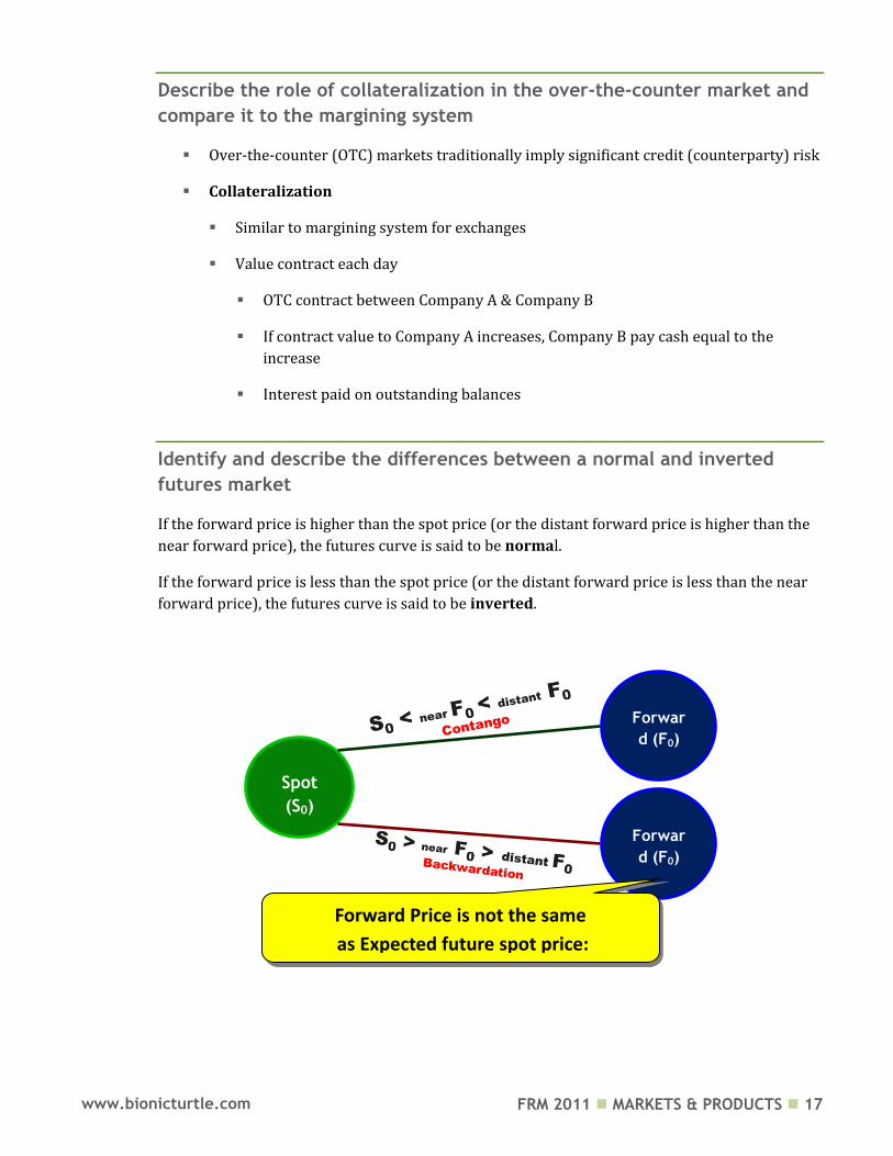
Identify and describe the differences between a normal and inverted
futures market
If the forward price is higher than the spot price (or the distant forward price is higher than the
near forward price), the futures curve is said to be normal.
If the forward price is less than the spot price (or the distant forward price is less than the near
forward price), the futures curve is said to be inverted.
Time (T)
Spot
(S0)
Forwar
d (F0)
Forwar
d (F0)
Forward Price is not the same
as Expected future spot price:
FRM 2011 MARKETS & PRODUCTS 18 www.bionicturtle.com
Describe the mechanics of the delivery process and contrast it with cash
settlement
If a futures contract is not closed out before maturity, it is usually settled by delivering the asset
underlying the contract.
When there are alternatives about what is delivered, where it is delivered, and when it is
delivered, the party with the short position chooses.
A few contracts (for example, those on stock indices and Eurodollars) are settled in cash
Define and demonstrate an understanding of the impact of different order
types, including: market, limit, stop‐loss, stop‐limit, market‐if‐touched,
discretionary, time‐of‐day, open, and fill‐or‐kill
Market order: immediate trade at best price
Limit order: specified price (or more favorable)
Stop-loss: once specified price is breached, immediate trade at best price
Stop-limit (combination of stop and limit): as soon as stop is breached, limit order
applies
Market-if-touched: best available price after a trade occurs at specified price (or better)
Discretionary: market order but may be delayed at broker’s discretion
Time-of-day: specifies a particular period of time during time
Open: in effect until executed or end of trading in contract
Fill-or-kill: immediately or not at all
Define:
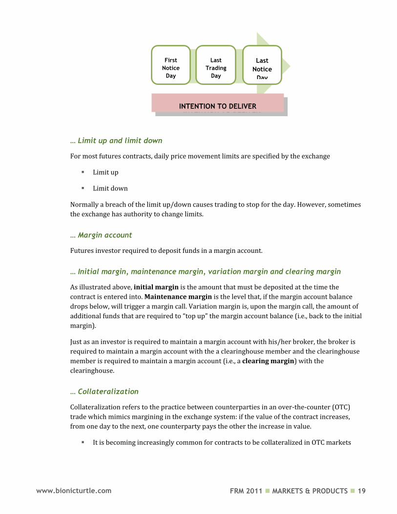
… Notice of intention to deliver
Sometimes the exchange allows for specified alternatives, in regard to grade of the asset and/or
delivery location, that satisfy the contract. When the party with the short position is ready to
deliver, it files a notice of intention to deliver with the exchange. This notice indicates selections
it has made with respect to the grade of the asset that will be delivered and the delivery location.
FRM 2011 MARKETS & PRODUCTS 19 www.bionicturtle.com
… Limit up and limit down
For most futures contracts, daily price movement limits are specified by the exchange
Limit up
Limit down
Normally a breach of the limit up/down causes trading to stop for the day. However, sometimes
the exchange has authority to change limits.
… Margin account
Futures investor required to deposit funds in a margin account.
… Initial margin, maintenance margin, variation margin and clearing margin
As illustrated above, initial margin is the amount that must be deposited at the time the
contract is entered into. Maintenance margin is the level that, if the margin account balance
drops below, will trigger a margin call. Variation margin is, upon the margin call, the amount of
additional funds that are required to “top up” the margin account balance (i.e., back to the initial
margin).
Just as an investor is required to maintain a margin account with his/her broker, the broker is
required to maintain a margin account with the a clearinghouse member and the clearinghouse
member is required to maintain a margin account (i.e., a clearing margin) with the
clearinghouse.
… Collateralization
Collateralization refers to the practice between counterparties in an over-the-counter (OTC)
trade which mimics margining in the exchange system: if the value of the contract increases,
from one day to the next, one counterparty pays the other the increase in value.
It is becoming increasingly common for contracts to be collateralized in OTC markets
First
Notice
Day
Last
Trading
Day
Last
Notice
Day
INTENTION TO DELIVER
FRM 2011 MARKETS & PRODUCTS 20 www.bionicturtle.com
They are then similar to futures contracts in that they are settled regularly (e.g. every day
or every week)
.. Open interest, settlement price and volume trading
Open interest: the total number of contracts outstanding
equal to number of long positions or number of short positions
Settlement price: the price just before the final bell each day
used for the daily settlement process
Volume of trading: the number of trades in 1 day
FRM 2011 MARKETS & PRODUCTS 21 www.bionicturtle.com
Hull, Chapter 3:
Hedging Strategies
Using Futures
In this chapter…
Define and differentiate between short and long hedges and identify situations where they are appropriate.
Describe the arguments for and against hedging and the potential impact of hedging on firm profitability.
Define and compute the basis. Define the various sources of basis risk and explain how basis risks arise when
hedging with futures. Define cross hedging. Define, compute and interpret the minimum variance hedge ratio and hedge
effectiveness. Define, compute and interpret the optimal number of futures contracts needed
to hedge an exposure, including a ―tailing the hedge‖ adjustment. Demonstrate how stock index futures contracts can be used to change a stock
portfolio’s beta. Describe what is meant by ―rolling the hedge forward‖ and discuss some of the
risks that arise from such a strategy.
Define and differentiate between short and long hedges and identify
situations where they are appropriate
A short forward (or futures) hedge is an agreement to sell in the future and is appropriate
when the hedger already owns the asset. The classic example is a farmer who wants to lock in a
sales price for his/her crop, and therefore protect him/herself against a price decline.
A long forward (or futures) hedge is an agreement to buy in the future and is appropriate
when the hedger does not currently own the asset but expects to purchase in the future. An
example is an airline which depends on jet fuel and enters into a forward or futures contract (a
long hedge) in order to protect itself from exposure to high oil prices.
FRM 2011 MARKETS & PRODUCTS 22 www.bionicturtle.com
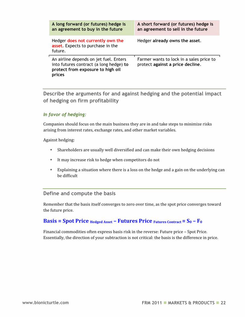
A long forward (or futures) hedge is an agreement to buy in the future
A short forward (or futures) hedge is an agreement to sell in the future
Hedger does not currently own the asset. Expects to purchase in the future.
Hedger already owns the asset.
An airline depends on jet fuel. Enters into futures contract (a long hedge) to protect from exposure to high oil prices
Farmer wants to lock in a sales price to protect against a price decline.
Describe the arguments for and against hedging and the potential impact
of hedging on firm profitability
In favor of hedging:
Companies should focus on the main business they are in and take steps to minimize risks
arising from interest rates, exchange rates, and other market variables.
Against hedging:
Shareholders are usually well diversified and can make their own hedging decisions
It may increase risk to hedge when competitors do not
Explaining a situation where there is a loss on the hedge and a gain on the underlying can
be difficult
Define and compute the basis
Remember that the basis itself converges to zero over time, as the spot price converges toward
the future price.
Basis = Spot Price Hedged Asset – Futures Price Futures Contract = S0 – F0
Financial commodities often express basis risk in the reverse: Future price – Spot Price.
Essentially, the direction of your subtraction is not critical: the basis is the difference in price.
FRM 2011 MARKETS & PRODUCTS 23 www.bionicturtle.com
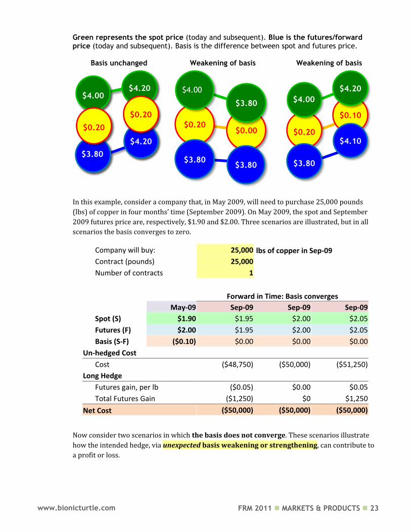
Green represents the spot price (today and subsequent). Blue is the futures/forward price (today and subsequent). Basis is the difference between spot and futures price.
Basis unchanged Weakening of basis Weakening of basis
In this example, consider a company that, in May 2009, will need to purchase 25,000 pounds
(lbs) of copper in four months’ time (September 2009). On May 2009, the spot and September
2009 futures price are, respectively, $1.90 and $2.00. Three scenarios are illustrated, but in all
scenarios the basis converges to zero.
Company will buy: 25,000 lbs of copper in Sep-09
Contract (pounds) 25,000
Number of contracts 1
Forward in Time: Basis converges
May-09 Sep-09 Sep-09 Sep-09
Spot (S) $1.90 $1.95 $2.00 $2.05
Futures (F) $2.00 $1.95 $2.00 $2.05
Basis (S-F) ($0.10) $0.00 $0.00 $0.00
Un-hedged Cost
Cost
($48,750) ($50,000) ($51,250)
Long Hedge
Futures gain, per lb ($0.05) $0.00 $0.05
Total Futures Gain ($1,250) $0 $1,250
Net Cost ($50,000) ($50,000) ($50,000)
Now consider two scenarios in which the basis does not converge. These scenarios illustrate
how the intended hedge, via unexpected basis weakening or strengthening, can contribute to
a profit or loss.
$3.80
$3.80
$4.00
$4.20
$4.20
$0.20
$0.20 $0.20
$0.00
$3.80
$4.00
$3.80
$3.80
$0.20
$0.10
$3.80
$4.00
$4.10
$4.20
FRM 2011 MARKETS & PRODUCTS 24 www.bionicturtle.com
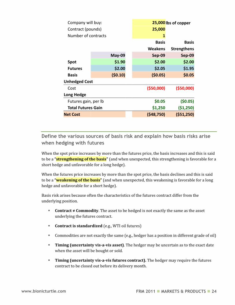
Company will buy:
25,000 lbs of copper
Contract (pounds)
25,000
Number of contracts
1
Basis Basis
Weakens Strengthens
May-09
Sep-09 Sep-09
Spot $1.90
$2.00 $2.00
Futures $2.00
$2.05 $1.95
Basis ($0.10)
($0.05) $0.05
Unhedged Cost
Cost
($50,000) ($50,000)
Long Hedge
Futures gain, per lb
$0.05 ($0.05)
Total Futures Gain
$1,250 ($1,250)
Net Cost ($48,750) ($51,250)
Define the various sources of basis risk and explain how basis risks arise
when hedging with futures
When the spot price increases by more than the futures price, the basis increases and this is said
to be a “strengthening of the basis” (and when unexpected, this strengthening is favorable for a
short hedge and unfavorable for a long hedge).
When the futures price increases by more than the spot price, the basis declines and this is said
to be a “weakening of the basis” (and when unexpected, this weakening is favorable for a long
hedge and unfavorable for a short hedge).
Basis risk arises because often the characteristics of the futures contract differ from the
underlying position.
Contract ≠ Commodity. The asset to be hedged is not exactly the same as the asset
underlying the futures contract.
Contract is standardized (e.g., WTI oil futures)
Commodities are not exactly the same (e.g., hedger has a position in different grade of oil)
Timing (uncertainty vis-a-vis asset). The hedger may be uncertain as to the exact date
when the asset will be bought or sold.
Timing (uncertainty vis-a-vis futures contract). The hedger may require the futures
contract to be closed out before its delivery month.
FRM 2011 MARKETS & PRODUCTS 25 www.bionicturtle.com
Basis risk may be sub-classified in various ways. For example, changes in the cost
of carry model, over time, may give rise to basis risk. But generally, any
particular type of basis risk reduces to one key fact: the asset being hedged is
typically not identical, in all respects, to the commodity underlying the futures
contract.
There is an inherent trade-off between liquidity and basis risk: to reduce basis risk is to require a
tailored hedge.
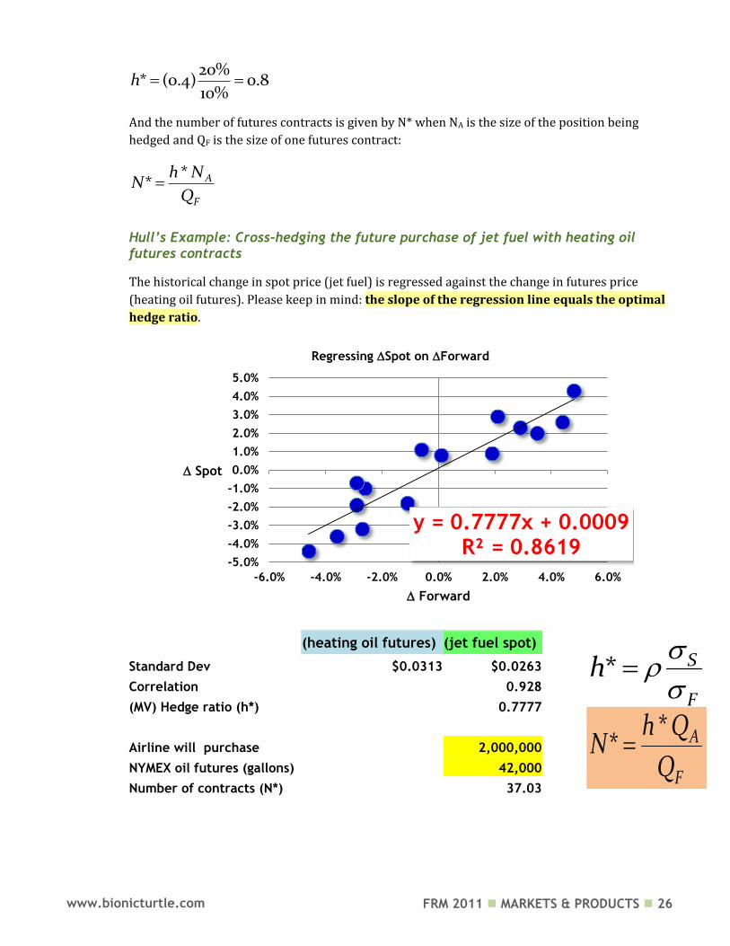
Define cross hedging
A cross hedge is when the asset underlying the hedge is different from the asset being hedged.
For example, an airline may hedge the cost of jet fuel with crude oil futures contracts. Cross-
hedges are necessary because futures are standardized contracts for commodities.
Define, compute and interpret the minimum variance hedge ratio and
hedge effectiveness
If the spot and future positions are perfectly correlated, then a 1:1 hedge ratio results in a perfect
hedge. However, this is not typically the case. The optimal hedge ratio (a.k.a., minimum variance
hedge ratio) is the ratio of futures position relative to the spot position that minimizes the
variance of the position.
Where is the correlation and is the standard deviation, the optimal hedge ratio is given by:
* S
F
h
For example, if the volatility of the spot price is 20%, the volatility of the futures price is 10%,
and their correlation is 0.4, then
TRADE OFF Basis Risk Liquidity
(Exchange)
FRM 2011 MARKETS & PRODUCTS 26 www.bionicturtle.com
20%* (0.4) 0.8
10%h
And the number of futures contracts is given by N* when NA is the size of the position being
hedged and QF is the size of one futures contract:
** A
F
h NN
Q
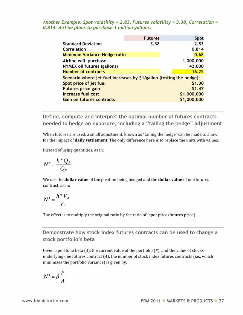
Hull’s Example: Cross-hedging the future purchase of jet fuel with heating oil futures contracts
The historical change in spot price (jet fuel) is regressed against the change in futures price
(heating oil futures). Please keep in mind: the slope of the regression line equals the optimal
hedge ratio.
(heating oil futures) (jet fuel spot)
Standard Dev $0.0313 $0.0263
Correlation
0.928
(MV) Hedge ratio (h*) 0.7777 0.78
Airline will purchase 2,000,000
NYMEX oil futures (gallons) 42,000
Number of contracts (N*) 37.03 37.01
y = 0.7777x + 0.0009 R² = 0.8619
-5.0%
-4.0%
-3.0%
-2.0%
-1.0%
0.0%
1.0%
2.0%
3.0%
4.0%
5.0%
-6.0% -4.0% -2.0% 0.0% 2.0% 4.0% 6.0%
Spot
Forward
Regressing Spot on Forward
*
* A
F
h QN
Q
* S
F
h
FRM 2011 MARKETS & PRODUCTS 27 www.bionicturtle.com
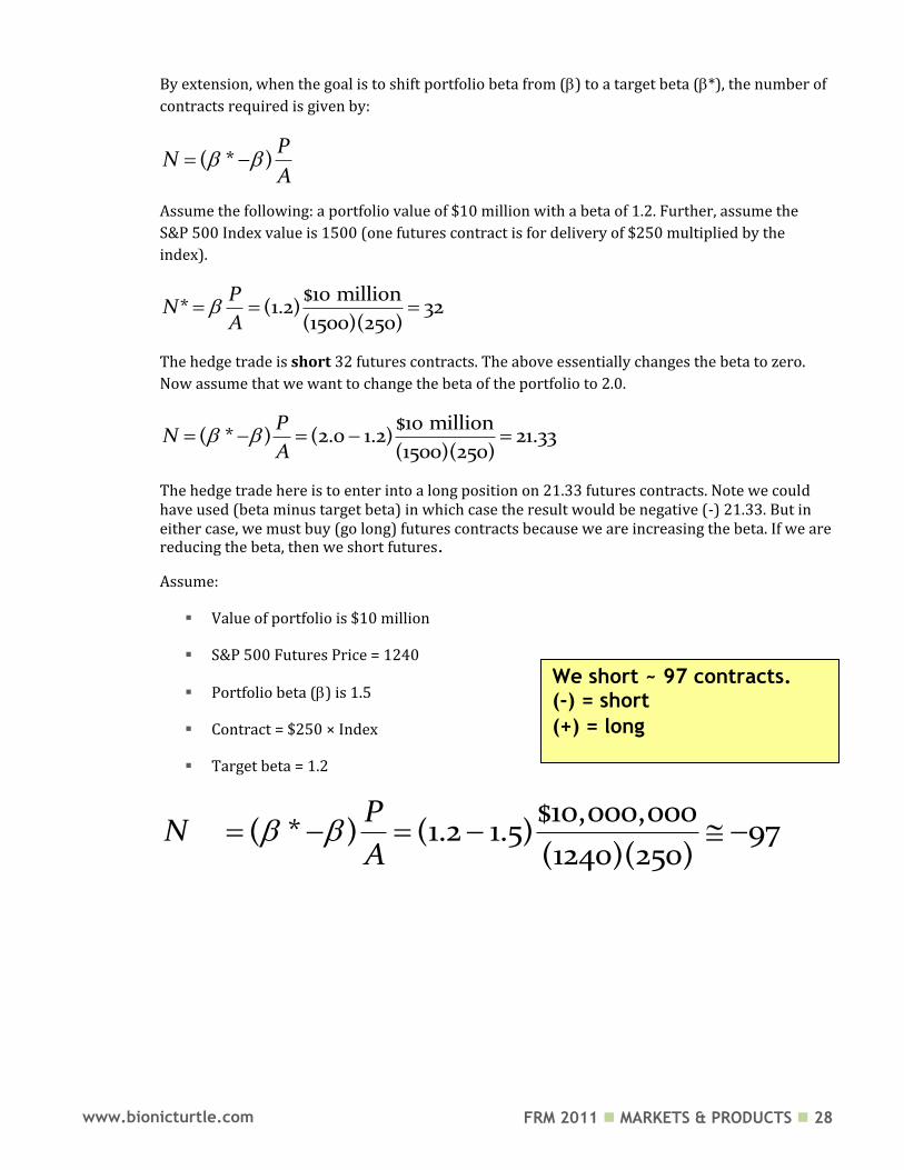
Another Example: Spot volatility = 2.83, Futures volatility = 3.38, Correlation = 0.814. Airline plans to purchase 1 million gallons.
Futures Spot
Standard Deviation 3.38 2.83
Correlation
0.814
Minimum Variance Hedge ratio 0.68
Airline will purchase 1,000,000
NYMEX oil futures (gallons) 42,000
Number of contracts 16.25
Scenario where jet fuel increases by $1/gallon (testing the hedge):
Spot price of jet fuel $1.00
Futures price gain $1.47
Increase fuel cost $1,000,000
Gain on futures contracts $1,000,000
Define, compute and interpret the optimal number of futures contracts
needed to hedge an exposure, including a ―tailing the hedge‖ adjustment
When futures are used, a small adjustment, known as “tailing the hedge” can be made to allow
for the impact of daily settlement. The only difference here is to replace the units with values.
Instead of using quantities, as in:
** A
F
h QN
Q
We use the dollar value of the position being hedged and the dollar value of one futures
contract, as in:
** A
F
h VN
V
The effect is to multiply the original ratio by the ratio of [spot price/futures price].
Demonstrate how stock index futures contracts can be used to change a
stock portfolio’s beta
Given a portfolio beta (), the current value of the portfolio (P), and the value of stocks
underlying one futures contract (A), the number of stock index futures contracts (i.e., which
minimizes the portfolio variance) is given by:
*P
NA
FRM 2011 MARKETS & PRODUCTS 28 www.bionicturtle.com
By extension, when the goal is to shift portfolio beta from () to a target beta (*), the number of
contracts required is given by:
( * )P
NA
Assume the following: a portfolio value of $10 million with a beta of 1.2. Further, assume the
S&P 500 Index value is 1500 (one futures contract is for delivery of $250 multiplied by the
index).
$10 million* (1.2) 32
(1500)(250)
PN
A
The hedge trade is short 32 futures contracts. The above essentially changes the beta to zero.
Now assume that we want to change the beta of the portfolio to 2.0.
$10 million( * ) (2.0 1.2) 21.33
(1500)(250)
PN
A
The hedge trade here is to enter into a long position on 21.33 futures contracts. Note we could have used (beta minus target beta) in which case the result would be negative (-) 21.33. But in either case, we must buy (go long) futures contracts because we are increasing the beta. If we are reducing the beta, then we short futures.
Assume:
Value of portfolio is $10 million
S&P 500 Futures Price = 1240
Portfolio beta () is 1.5
Contract = $250 × Index
Target beta = 1.2
$10,000,000( * ) (1.2 1.5) 97
(1240)(250)
PN
A
We short ~ 97 contracts. (-) = short
(+) = long
FRM 2011 MARKETS & PRODUCTS 29 www.bionicturtle.com
Describe what is meant by ―rolling the hedge forward‖ and discuss some
of the risks that arise from such a strategy
When the delivery date of the futures contract occurs prior to the expiration date of the hedge,
the hedger can roll forward the hedge: close out a futures contract and take the same position on
a new futures contract with a later delivery date.
Rolling the hedge is exposed to:
Basis risk (original hedge)
Basis risk (each new hedge) = also called “rollover basis risk”
FRM 2011 MARKETS & PRODUCTS 30 www.bionicturtle.com
Hull, Chapter 4:
Interest Rates
In this chapter…
Calculate the value of an investment using daily, weekly, monthly, quarterly, semiannual, annual, and continuous compounding. Convert rates based on different compounding frequencies.
Calculate the theoretical price of a coupon paying bond using spot rates. Calculate forward interest rates from a set of spot rates. Value and calculate the cash flows from a forward rate agreement (FRA). Describe the limitations of duration and how convexity addresses some of them. Calculate the change in a bond’s price given duration, convexity, and a change
in interest rates. Define and discuss the major theories of the term structure of interest rates. Define:
Spot rate Par yield Bootstrap method Forward rate agreement Basis point Duration Modified duration Dollar duration Convexity
Calculate the value of an investment using daily, weekly, monthly,
quarterly, semi-annual, annual, and continuous compounding.
Assuming:
R c: rate of interest with continuous compounding
R m
: rate of interest with discrete compounding (m per annum)
n: number of years
FRM 2011 MARKETS & PRODUCTS 31 www.bionicturtle.com
1
1
mnR n mc
mR mc
RAe A
m
Re
m
/ 1
ln 1
R mcm
mc
R m e
RR m
m
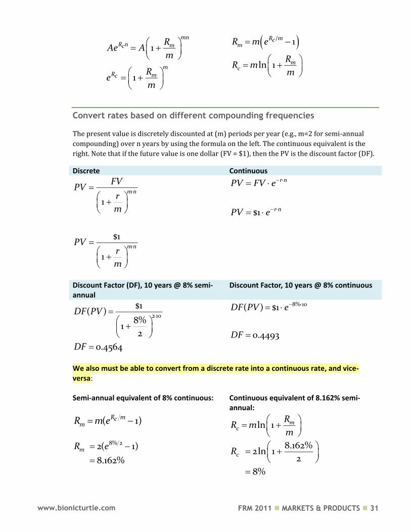
Convert rates based on different compounding frequencies
The present value is discretely discounted at (m) periods per year (e.g., m=2 for semi-annual
compounding) over n years by using the formula on the left. The continuous equivalent is the
right. Note that if the future value is one dollar (FV = $1), then the PV is the discount factor (DF).
Discrete Continuous
1
$1
1
mn
mn
FVPV
r
m
PVr
m
$1
r n
r n
PV FV e
PV e
Discount Factor (DF), 10 years @ 8% semi-annual
Discount Factor, 10 years @ 8% continuous
2 10
$1( )
8%1
2
0.4564
DF PV
DF
8% 10( ) $1
0.4493
DF PV e
DF
We also must be able to convert from a discrete rate into a continuous rate, and vice-versa: Semi-annual equivalent of 8% continuous: Continuous equivalent of 8.162% semi-
annual:
( 1)R mcmR m e ln 1 m
c
RR m
m
8% 22( 1)
8.162%mR e
8.162%2ln 1
2
8%
cR
FRM 2011 MARKETS & PRODUCTS 32 www.bionicturtle.com
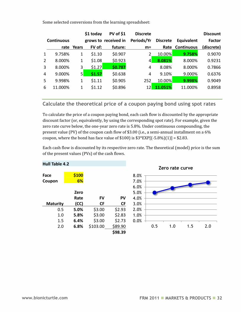
Some selected conversions from the learning spreadsheet:
$1 today PV of $1
Discrete
Discount
Continuous
grows to received in
Periods/Yr Discrete Equivalent Factor
rate Years FV of: future: m= Rate Continuous (discrete)
1 9.758% 1 $1.10 $0.907
2 10.00% 9.758% 0.9070
2 8.000% 1 $1.08 $0.923
4 8.081% 8.000% 0.9231
3 8.000% 3 $1.27 $0.787
4 8.08% 8.000% 0.7866
4 9.000% 5 $1.57 $0.638
4 9.10% 9.000% 0.6376
5 9.998% 1 $1.11 $0.905
252 10.00% 9.998% 0.9049
6 11.000% 1 $1.12 $0.896
12 11.051% 11.000% 0.8958
Calculate the theoretical price of a coupon paying bond using spot rates
To calculate the price of a coupon paying bond, each cash flow is discounted by the appropriate
discount factor (or, equivalently, by using the corresponding spot rate). For example, given the
zero rate curve below, the one-year zero rate is 5.8%. Under continuous compounding, the
present value (PV) of the coupon cash flow of $3.00 (i.e., a semi-annual installment on a 6%
coupon, where the bond has face value of $100) is $3*EXP[(-5.8%)(1)] = $2.83.
Each cash flow is discounted by its respective zero rate. The theoretical (model) price is the sum
of the present values (PVs) of the cash flows.
Hull Table 4.2
Face $100
Coupon 6%
Zero
Rate FV PV
Maturity (CC) CF CF 0.5 5.0% $3.00 $2.93 1.0 5.8% $3.00 $2.83 1.5 6.4% $3.00 $2.73 2.0 6.8% $103.00 $89.90
$98.39
0.0%
1.0%
2.0%
3.0%
4.0%
5.0%
6.0%
7.0%
8.0%
0.5 1.0 1.5 2.0
Zero rate curve
FRM 2011 MARKETS & PRODUCTS 33 www.bionicturtle.com
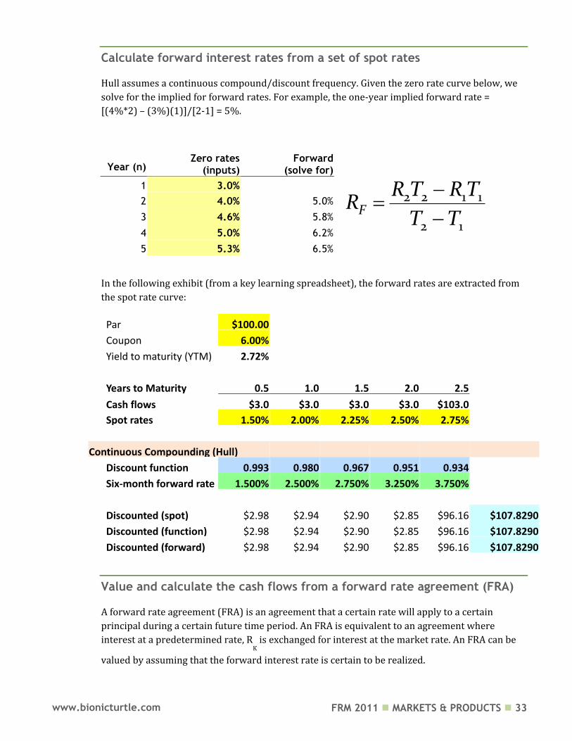
Calculate forward interest rates from a set of spot rates
Hull assumes a continuous compound/discount frequency. Given the zero rate curve below, we
solve for the implied for forward rates. For example, the one-year implied forward rate =
[(4%*2) – (3%)(1)]/[2-1] = 5%.
Year (n) Zero rates
(inputs) Forward
(solve for)
1 3.0%
2 4.0% 5.0%
3 4.6% 5.8%
4 5.0% 6.2%
5 5.3% 6.5%
In the following exhibit (from a key learning spreadsheet), the forward rates are extracted from
the spot rate curve:
Par
$100.00
Coupon 6.00%
Yield to maturity (YTM) 2.72%
Years to Maturity 0.5 1.0 1.5 2.0 2.5
Cash flows $3.0 $3.0 $3.0 $3.0 $103.0
Spot rates 1.50% 2.00% 2.25% 2.50% 2.75%
Continuous Compounding (Hull)
Discount function 0.993 0.980 0.967 0.951 0.934
Six-month forward rate 1.500% 2.500% 2.750% 3.250% 3.750%
Discounted (spot) $2.98 $2.94 $2.90 $2.85 $96.16 $107.8290
Discounted (function) $2.98 $2.94 $2.90 $2.85 $96.16 $107.8290
Discounted (forward) $2.98 $2.94 $2.90 $2.85 $96.16 $107.8290
Value and calculate the cash flows from a forward rate agreement (FRA)
A forward rate agreement (FRA) is an agreement that a certain rate will apply to a certain
principal during a certain future time period. An FRA is equivalent to an agreement where
interest at a predetermined rate, RK is exchanged for interest at the market rate. An FRA can be
valued by assuming that the forward interest rate is certain to be realized.
2 2 1 1
2 1F
R T RTR
T T
FRM 2011 MARKETS & PRODUCTS 34 www.bionicturtle.com
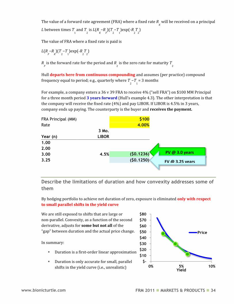
The value of a forward rate agreement (FRA) where a fixed rate RK will be received on a principal
L between times T1
and T2 is L(R
K−R
F)(T
2−T
1)exp(-R
2T
2)
The value of FRA where a fixed rate is paid is
L(RF−R
K)(T
2−T
1)exp(-R
2T
2)
RF is the forward rate for the period and R
2 is the zero rate for maturity T
2
Hull departs here from continuous compounding and assumes (per practice) compound
frequency equal to period; e.g., quarterly where T2−T
1 = 3 months
For example, a company enters a 36 v 39 FRA to receive 4% (“sell FRA”) on $100 MM Principal
for a three month period 3 years forward (Hull’s example 4.3). The other interpretation is that
the company will receive the fixed rate (4%) and pay LIBOR. If LIBOR is 4.5% in 3 years,
company ends up paying. The counterparty is the buyer and receives the payment.
FRA Principal (MM) $100
Rate
4.00%
3 Mo.
Year (n) LIBOR
1.00
2.00
3.00 4.5% ($0.1236)
3.25
($0.1250)
Describe the limitations of duration and how convexity addresses some of
them
By hedging portfolio to achieve net duration of zero, exposure is eliminated only with respect
to small parallel shifts in the yield curve
We are still exposed to shifts that are large or
non-parallel. Convexity, as a function of the second
derivative, adjusts for some but not all of the
“gap” between duration and the actual price change.
In summary:
Duration is a first-order linear approximation
Duration is only accurate for small, parallel
shifts in the yield curve (i.e., unrealistic)
$-
$10
$20
$30
$40
$50
$60
$70
$80
0% 5% 10%Yield
Price
PV @ 3.0 years Basis risk
FV @ 3.25 years
FRM 2011 MARKETS & PRODUCTS 35 www.bionicturtle.com
Convexity adds a term to adjust for the
curvature in the price/yield curve
Convexity is still imprecise
Both utilize the Taylor Series approximation: duration is the first term (or is a function of
the first term) and convexity is (a function of) the second term.
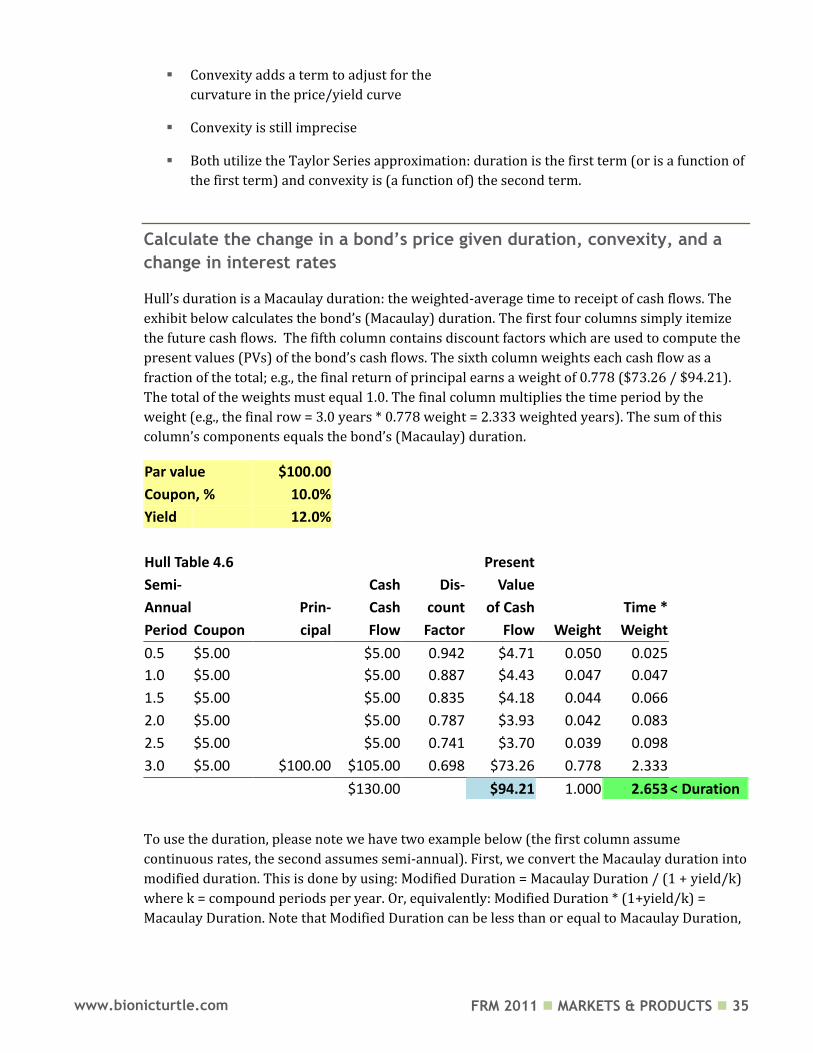
Calculate the change in a bond’s price given duration, convexity, and a
change in interest rates
Hull’s duration is a Macaulay duration: the weighted-average time to receipt of cash flows. The
exhibit below calculates the bond’s (Macaulay) duration. The first four columns simply itemize
the future cash flows. The fifth column contains discount factors which are used to compute the
present values (PVs) of the bond’s cash flows. The sixth column weights each cash flow as a
fraction of the total; e.g., the final return of principal earns a weight of 0.778 ($73.26 / $94.21).
The total of the weights must equal 1.0. The final column multiplies the time period by the
weight (e.g., the final row = 3.0 years * 0.778 weight = 2.333 weighted years). The sum of this
column’s components equals the bond’s (Macaulay) duration.
Par value $100.00
Coupon, % 10.0%
Yield 12.0%
Hull Table 4.6
Present
Semi-
Cash Dis- Value
Annual
Prin- Cash count of Cash
Time *
Period Coupon cipal Flow Factor Flow Weight Weight
0.5 $5.00
$5.00 0.942 $4.71 0.050 0.025
1.0 $5.00
$5.00 0.887 $4.43 0.047 0.047
1.5 $5.00
$5.00 0.835 $4.18 0.044 0.066
2.0 $5.00
$5.00 0.787 $3.93 0.042 0.083
2.5 $5.00
$5.00 0.741 $3.70 0.039 0.098
3.0 $5.00 $100.00 $105.00 0.698 $73.26 0.778 2.333
$130.00
$94.21 1.000 2.653 < Duration
To use the duration, please note we have two example below (the first column assume
continuous rates, the second assumes semi-annual). First, we convert the Macaulay duration into
modified duration. This is done by using: Modified Duration = Macaulay Duration / (1 + yield/k)
where k = compound periods per year. Or, equivalently: Modified Duration * (1+yield/k) =
Macaulay Duration. Note that Modified Duration can be less than or equal to Macaulay Duration,
FRM 2011 MARKETS & PRODUCTS 36 www.bionicturtle.com
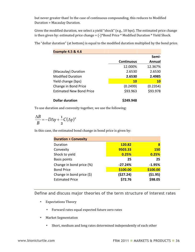
but never greater than! In the case of continuous compounding, this reduces to Modified
Duration = Macaulay Duration.
Given the modified duration, we select a yield “shock” (e.g., 10 bps). The estimated price change
is then given by: estimated price change = (-)*Bond Price * Modified Duration * Yield Shock.
The “dollar duration” (at bottom) is equal to the modified duration multiplied by the bond price.
Example 4.5 & 4.6
Semi-
Continuous Annual
12.000% 12.367%
(Macaulay) Duration 2.6530 2.6530
Modified Duration
2.6530 2.4985
Yield change (bps)
10 10
Change in Bond Price (0.2499) (0.2354)
Estimated New Bond Price $93.963 $93.978
Dollar duration
$249.948
To use duration and convexity together, we use the following:
21( )
2
BD y C y
B
In this case, the estimated bond change in bond price is given by:
Duration + Convexity
Duration
120.82 8
Convexity
9503.33 150
Shock to yield
0.25% 0.25%
Basis points
25 25
Change in bond price (%) -27.24% -1.95%
Bond Price
$100.00 $100.00
Change in bond price ($) ($27.24) ($1.95)
Estimated Price
$72.76 $98.05
Define and discuss major theories of the term structure of interest rates
Expectations Theory
Forward rates equal expected future zero rates
Market Segmentation
Short, medium and long rates determined independently of each other
FRM 2011 MARKETS & PRODUCTS 37 www.bionicturtle.com
Liquidity Preference Theory
Forward rates higher than expected future zero rates
Define:
Spot rate
A zero rate (or spot rate), for maturity T is the rate of interest earned on an investment that
provides a payoff only at time T.
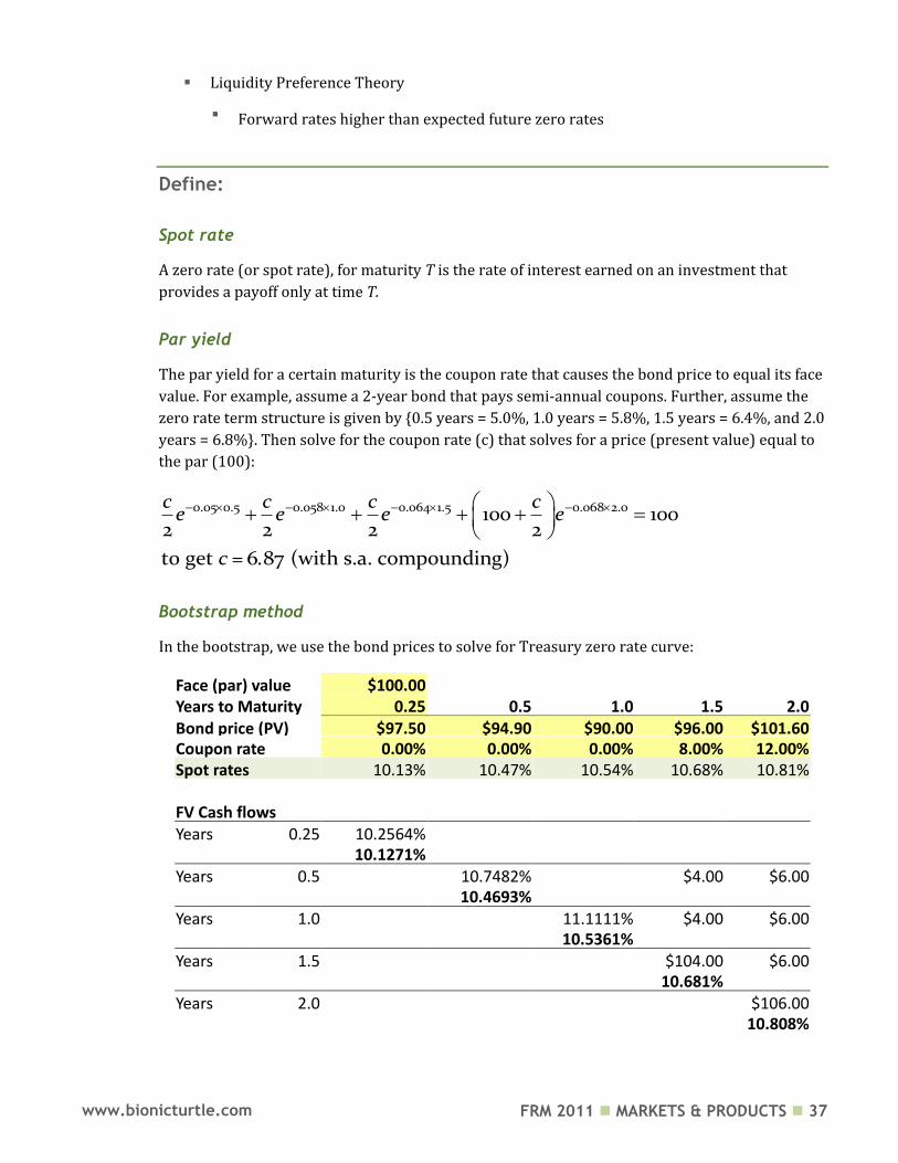
Par yield
The par yield for a certain maturity is the coupon rate that causes the bond price to equal its face
value. For example, assume a 2-year bond that pays semi-annual coupons. Further, assume the
zero rate term structure is given by {0.5 years = 5.0%, 1.0 years = 5.8%, 1.5 years = 6.4%, and 2.0
years = 6.8%}. Then solve for the coupon rate (c) that solves for a price (present value) equal to
the par (100):
0.05 0.5 0.058 1.0 0.064 1.5 0.068 2.0100 1002 2 2 2
to get 6 87 (with s.a. compounding)
c c c ce e e e
c = .
Bootstrap method
In the bootstrap, we use the bond prices to solve for Treasury zero rate curve:
Face (par) value $100.00
Years to Maturity 0.25 0.5 1.0 1.5 2.0 Bond price (PV) $97.50 $94.90 $90.00 $96.00 $101.60 Coupon rate 0.00% 0.00% 0.00% 8.00% 12.00% Spot rates 10.13% 10.47% 10.54% 10.68% 10.81%
FV Cash flows
Years 0.25 10.2564%
10.1271%
Years 0.5 10.7482% $4.00 $6.00
10.4693%
Years 1.0 11.1111% $4.00 $6.00
10.5361%
Years 1.5 $104.00 $6.00
10.681%
Years 2.0 $106.00
10.808%
FRM 2011 MARKETS & PRODUCTS 38 www.bionicturtle.com
Forward rate agreement
A forward rate agreement (FRA) is an agreement that a certain rate will apply to a certain
principal during a certain future time period
An FRA is equivalent to an agreement where interest at a predetermined rate, RK is exchanged
for interest at the market rate
An FRA can be valued by assuming that the forward interest rate is certain to be realized.
Yield
The bond yield is also known as the yield to maturity (YTM). The yield (YTM) is the discount
rate that makes the present value of the cash flows on the bond equal to the market price of the
bond
Suppose that the market price of the bond in our example equals its theoretical price of 98.39
The bond yield (continuously compounded) is given by solving
0.5 1.0 1.5 2.03 3 3 103 98.39y y y ye e e e
to get y=0.0676 or 6.76%.
Basis point
One basis point is equal to 1/100th of one percent, such that 100 basis points = 1.0%.
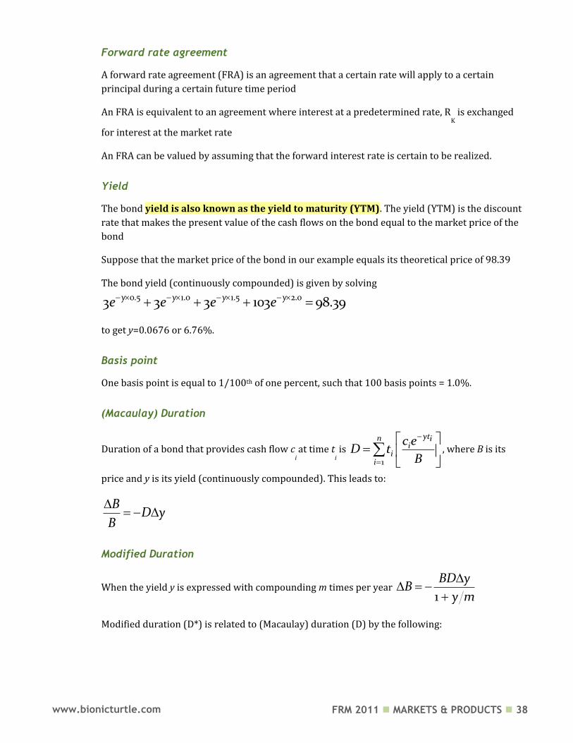
(Macaulay) Duration
Duration of a bond that provides cash flow ci at time t
i is
1
ytn ii
ii
c eD t
B
, where B is its
price and y is its yield (continuously compounded). This leads to:
BD y
B
Modified Duration
When the yield y is expressed with compounding m times per year 1
BD yB
y m
Modified duration (D*) is related to (Macaulay) duration (D) by the following:
FRM 2011 MARKETS & PRODUCTS 39 www.bionicturtle.com
*1
DD
y m
Such that the estimated change in bond price is a function of the modified duration:
*B BD y
Modified duration is the measure of sensitivity, so it is typically more useful to
us than Macaulay Duration. Macaulay duration is convenient, however, because a
zero-coupon bond has a Macualay duration equal to its term to maturity; e.g., a
10-year zero has Macalauy duration of ten and modified duration of (slightly)
less than 10.
Dollar duration
Dollar duration (DD**), also known as value duration, is the slope of the tangent line (a first
partial derivative)
*
* * *
* *
B BD y
D BD
B D y
We use dollar/value duration to aggregate components in a portfolio. For
example, to hedge a bond position with dollar duration of -1000, we will seek an
offsetting position with dollar duration of +1000. It is difficult to aggregate with
modified of Macaulay durations.
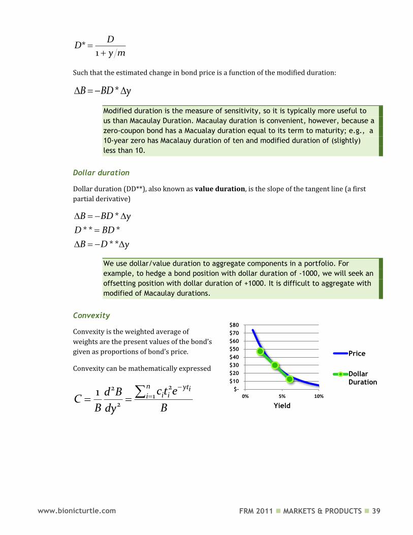
Convexity
Convexity is the weighted average of maturity-squares of a bond, where
weights are the present values of the bond’s cash flows,
given as proportions of bond’s price.
Convexity can be mathematically expressed
221
2
1n yti
i iic t ed B
CB Bdy
$-
$10
$20
$30
$40
$50
$60
$70
$80
0% 5% 10%
Yield
Price
DollarDuration
FRM 2011 MARKETS & PRODUCTS 40 www.bionicturtle.com
Hull, Chapter 5:
Determination of
Forward and
Futures Prices
In this chapter…
Differentiate between investment and consumption assets. Define short‐selling and short squeeze. Discuss the differences between forward and futures contracts and explain the
relationship between forward and spot prices. Calculate the forward price, given the underlying asset’s price, with or without
short sales and/or consideration to the income or yield of the underlying asset. Describe an arbitrage argument in support of these prices.
Explain the relationship between forward and futures prices. Use the interest rate parity relationship to calculate a forward foreign exchange
rate. Define income, storage costs, and convenience yield. Calculate the futures price on commodities incorporating storage costs and/or
convenience yields. Define and calculate, using the cost‐of‐carry model, forward prices where the
underlying asset either does or does not have interim cash flows. Discuss the various delivery options available in the futures markets and how
they can influence futures prices. Analyze the relationship between current futures prices and expected future
spot prices, including the impact of systematic and nonsystematic risk. Define contango and backwardation, interpret the effect contango or
backwardation may have on the relationship between commodity futures and spot prices, and relate the cost‐of‐carry model to contango and backwardation.
Differentiate between investment and consumption assets
An investment asset is an asset that is held for investment purposes by significant numbers of
investors; e.g., stocks, bonds, gold, silver.
A consumption asset is held primarily for consumption; e.g., copper, oil, pork bellies, silver.
Note: silver is an example of both.
FRM 2011 MARKETS & PRODUCTS 41 www.bionicturtle.com
Investment Consumption
[Theory] No-arbitrage implies forward is a function of spot price
Because of convenience yield, forward price is not a simple function of spot
Define short‐selling and short squeeze
In a short sale, the investor wants to profit from a decline in the price of the security. The short-
seller borrows shares of stock from the broker in order to sell the shares. Subsequently, the
short-seller purchases the shares in order to replace the borrowed shares. This is known as
covering the short position.
But the short-seller can experience a short squeeze. In a short-squeeze, the contract is open, the
broker runs out of shares to borrow, and the investor is forced to cover (close out) position
Time Cash Flow
0 Borrow shares, Sell shares + Price
1 Pay dividend - Dividend
2 Buy shares to close short position - Ending Price
Discuss the differences between forward and futures contracts and
explain the relationship between forward and spot prices
Differences between forward and futures contracts
While both forwards and futures are agreements to buy or sell an asset in the future (at a
specified price), a forward contract is traded over-the-counter and the forward is not
standardized. The futures contract is traded on an exchange, standardized (often highly
standardized) and typically closed out before maturity.
FRM 2011 MARKETS & PRODUCTS 42 www.bionicturtle.com
Forward vs. Futures Contracts
Forward Futures
Trade over-the-counter Trade on an exchange
Not standardized Standardized contracts
One specified delivery date Range of delivery dates
Settled at the end of a contract Settled daily
Delivery or final cash settlement usually occurs
Contract usually closed out prior to maturity
… Explain the relationship between forward and spot prices
Notation
The following notations apply to forward contracts:
T: Time until delivery date in a forward/futures contract (in years) S0: Price of the underlying asset (spot price) F0: Today’s forward or futures price K: Delivery price r: Risk-free rate—annual rate but expressed with continuous compounding rf: Foreign risk-free interest rate I: Present value of income received from asset (in dollar terms) q: Dividend yield rate (in percentage terms; e.g., 2% dividend yield) U, u: Storage cost. U = dollar cost and u = cost in % terms y: convenience yield
Cost of Carry Model
The cost-of-carry model sets a futures price as a function of the spot price: the futures price (F)
equals the spot price (S0) compounded at the interest rate (r, required to finance the asset) plus
the storage cost of the asset less any income earned on the asset.
For a non-dividend-paying investment asset (i.e., an asset which has no storage cost) the cost
of carry model says the futures price is given by:
0 0 0 0cT rTF S e F S e
The equations for forward prices are essentially similar to futures prices. The generalized
forward price (F0) is either case (futures or forwards) is therefore given by:
0 0rTF S e
If the asset provides interim cash flows (e.g., a stock that pays dividends), then let (I) equal
the present value of the cash flows received and the cost-of-carry model is then given by:
0 0( ) rTF S I e
FRM 2011 MARKETS & PRODUCTS 43 www.bionicturtle.com
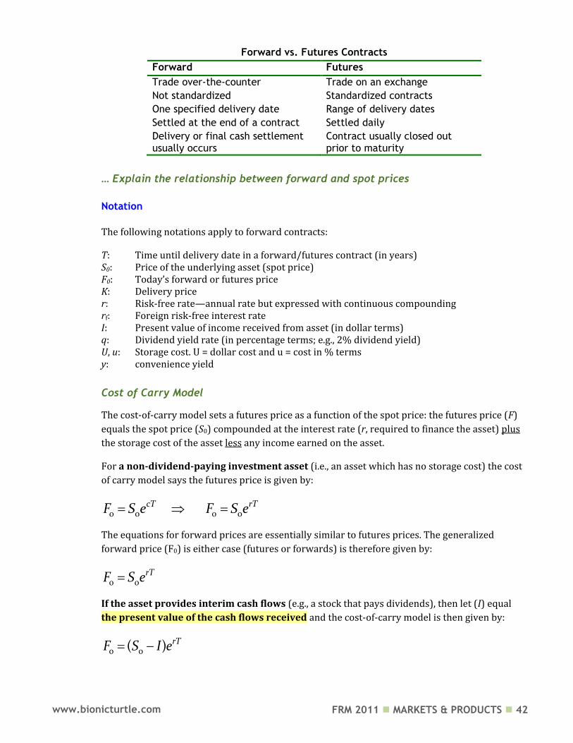
If the asset provides income (e.g., a stock that pays dividends), where the income can be
expressed as a constant percentage of the spot price (given by q), then the model is given by:
( )0 0
r q TF S e
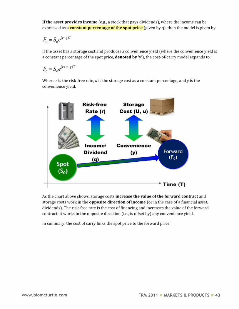
If the asset has a storage cost and produces a convenience yield (where the convenience yield is
a constant percentage of the spot price, denoted by ‘y’), the cost-of-carry model expands to:
( )0 0
r u y TF S e
Where r is the risk-free rate, u is the storage cost as a constant percentage, and y is the
convenience yield.
As the chart above shows, storage costs increase the value of the forward contract and
storage costs work in the opposite direction of income (or in the case of a financial asset,
dividends). The risk-free rate is the cost of financing and increases the value of the forward
contract; it works in the opposite direction (i.e., is offset by) any convenience yield.
In summary, the cost of carry links the spot price to the forward price:
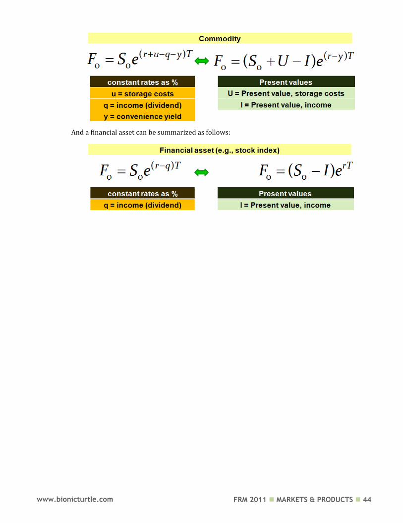
FRM 2011 MARKETS & PRODUCTS 44 www.bionicturtle.com
And a financial asset can be summarized as follows:
FRM 2011 MARKETS & PRODUCTS 45 www.bionicturtle.com
Calculate the forward price, given the underlying asset’s price, with or
without short sales and/or consideration to the income or yield of the
underlying asset. Describe an arbitrage argument in support of these
prices
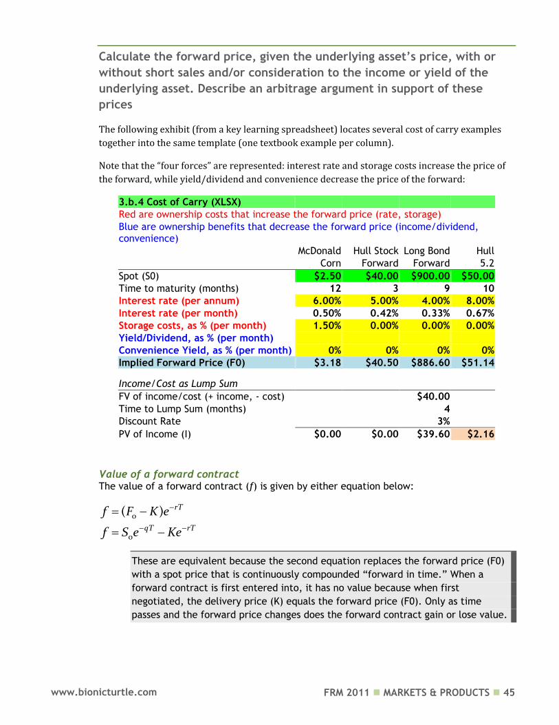
The following exhibit (from a key learning spreadsheet) locates several cost of carry examples
together into the same template (one textbook example per column).
Note that the “four forces” are represented: interest rate and storage costs increase the price of
the forward, while yield/dividend and convenience decrease the price of the forward:
3.b.4 Cost of Carry (XLSX) Red are ownership costs that increase the forward price (rate, storage)
Blue are ownership benefits that decrease the forward price (income/dividend, convenience)
McDonald Hull Stock Long Bond Hull
Corn Forward Forward 5.2
Spot (S0) $2.50 $40.00 $900.00 $50.00
Time to maturity (months) 12 3 9 10
Interest rate (per annum) 6.00% 5.00% 4.00% 8.00%
Interest rate (per month) 0.50% 0.42% 0.33% 0.67%
Storage costs, as % (per month) 1.50% 0.00% 0.00% 0.00%
Yield/Dividend, as % (per month)
Convenience Yield, as % (per month) 0% 0% 0% 0%
Implied Forward Price (F0) $3.18 $40.50 $886.60 $51.14
Income/Cost as Lump Sum
FV of income/cost (+ income, - cost)
$40.00
Time to Lump Sum (months)
4
Discount Rate
3%
PV of Income (I) $0.00 $0.00 $39.60 $2.16
Value of a forward contract The value of a forward contract (f) is given by either equation below:
0
0
( ) rT
qT rT
f F K e
f S e Ke
These are equivalent because the second equation replaces the forward price (F0)
with a spot price that is continuously compounded “forward in time.” When a
forward contract is first entered into, it has no value because when first
negotiated, the delivery price (K) equals the forward price (F0). Only as time
passes and the forward price changes does the forward contract gain or lose value.
FRM 2011 MARKETS & PRODUCTS 46 www.bionicturtle.com
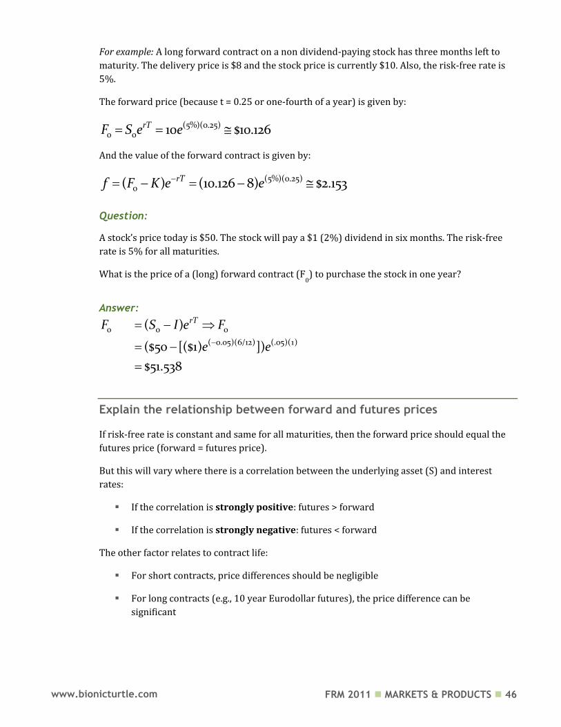
For example: A long forward contract on a non dividend-paying stock has three months left to
maturity. The delivery price is $8 and the stock price is currently $10. Also, the risk-free rate is
5%.
The forward price (because t = 0.25 or one-fourth of a year) is given by:
(5%)(0.25)0 0 10 $10.126rTF S e e
And the value of the forward contract is given by:
(5%)(0.25)0( ) (10.126 8) $2.153rTf F K e e
Question:
A stock’s price today is $50. The stock will pay a $1 (2%) dividend in six months. The risk-free
rate is 5% for all maturities.
What is the price of a (long) forward contract (F0) to purchase the stock in one year?
Answer:
0 0 0
( 0.05)(6/12) (.05)(1)
( )
($50 [($1) ])
$51.538
rTF S I e F
e e
Explain the relationship between forward and futures prices
If risk-free rate is constant and same for all maturities, then the forward price should equal the
futures price (forward = futures price).
But this will vary where there is a correlation between the underlying asset (S) and interest
rates:
If the correlation is strongly positive: futures > forward
If the correlation is strongly negative: futures < forward
The other factor relates to contract life:
For short contracts, price differences should be negligible
For long contracts (e.g., 10 year Eurodollar futures), the price difference can be
significant
FRM 2011 MARKETS & PRODUCTS 47 www.bionicturtle.com
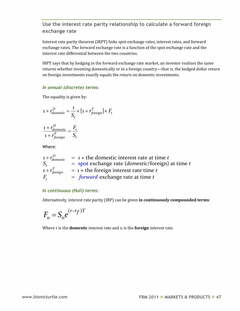
Use the interest rate parity relationship to calculate a forward foreign
exchange rate
Interest rate parity theorem (IRPT) links spot exchange rates, interest rates, and forward
exchange rates. The forward exchange rate is a function of the spot exchange rate and the
interest rate differential between the two countries.
IRPT says that by hedging in the forward exchange rate market, an investor realizes the same
returns whether investing domestically or in a foreign country—that is, the hedged dollar return
on foreign investments exactly equals the return on domestic investments.
In annual (discrete) terms:
The equality is given by:
11 [1 ]D F
domestic foreign tt
r r FS
1
1
Ddomestic tF
tforeign
r F
Sr
Where:
1 1 + the domestic interest rate at time exchange rate ( /foreign) at time
1 1 + the foreign interest rate tspot
ime exchange rate at time
Ddomestic
tFforeign
t
r tS domestic t
r tF tforward
In continuous (Hull) terms:
Alternatively, interest rate parity (IRP) can be given in continuously compounded terms:
( )
0 0
r r TfF S e
Where r is the domestic interest rate and rf is the foreign interest rate.
FRM 2011 MARKETS & PRODUCTS 48 www.bionicturtle.com
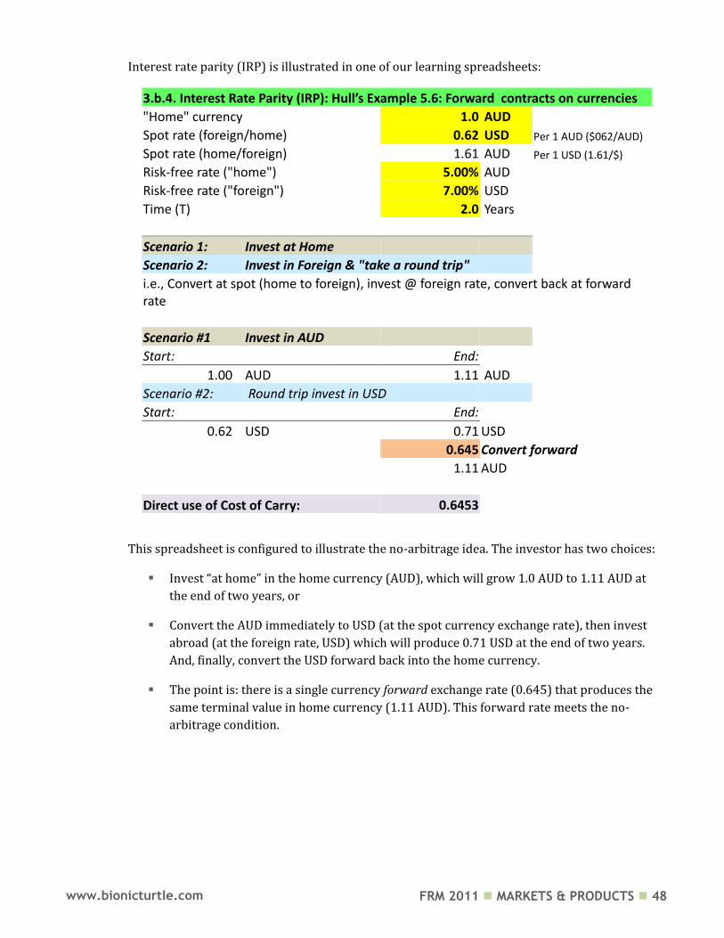
Interest rate parity (IRP) is illustrated in one of our learning spreadsheets:
3.b.4. Interest Rate Parity (IRP): Hull’s Example 5.6: Forward contracts on currencies
"Home" currency
1.0 AUD Spot rate (foreign/home)
0.62 USD Per 1 AUD ($062/AUD)
Spot rate (home/foreign)
1.61 AUD Per 1 USD (1.61/$)
Risk-free rate ("home")
5.00% AUD Risk-free rate ("foreign")
7.00% USD
Time (T)
2.0 Years
Scenario 1: Invest at Home Scenario 2: Invest in Foreign & "take a round trip" i.e., Convert at spot (home to foreign), invest @ foreign rate, convert back at forward
rate
Scenario #1 Invest in AUD
Start:
End: 1.00 AUD 1.11 AUD
Scenario #2: Round trip invest in USD Start: End:
0.62 USD
0.71 USD
0.645 Convert forward
1.11 AUD
Direct use of Cost of Carry: 0.6453
This spreadsheet is configured to illustrate the no-arbitrage idea. The investor has two choices:
Invest “at home” in the home currency (AUD), which will grow 1.0 AUD to 1.11 AUD at
the end of two years, or
Convert the AUD immediately to USD (at the spot currency exchange rate), then invest
abroad (at the foreign rate, USD) which will produce 0.71 USD at the end of two years.
And, finally, convert the USD forward back into the home currency.
The point is: there is a single currency forward exchange rate (0.645) that produces the
same terminal value in home currency (1.11 AUD). This forward rate meets the no-
arbitrage condition.
FRM 2011 MARKETS & PRODUCTS 49 www.bionicturtle.com
Define income, storage costs, and convenience yield
Income refers to a commodity that pays cash the owner (holder) of the asset; the party who is
long the futures or forward contract forgoes the income. Examples include:
Stocks paying known dividends
Coupon-bearing bonds
Storage costs are the cost to store or carry the asset; storage costs are typically associated with
physical commodities.
Convenience Yield
The convenience yield reflects the “excess benefits” conferred by taking physical ownership
of the asset (i.e., as opposed to holding a futures contract). The convenience yield is generally
not relevant for financial assets. But for commodities (physical assets), ownership may confer
positive benefits or may decrease perceived risk.
The convenience yield is the “plug variable” that validates the cost of carry model. The
convenience yield impounds benefits of holding/owning the physical asset. This includes any
real optimality benefits of commodity ownership (i.e., owning the asset gives the owner some
future real option).
For a consumption asset—where (y) is the convenience yield and (c) is the cost of carry—the
futures price is given by:
( )0 0
c y TF S e
Note this is essentially similar to the forward price if we replace the cost of carry (c) with the
risk-free rate (r).
If a non dividend-paying stock offered a “convenience yield” then its forward price calculation
would mirror the above formula:
( )0 0
r y TF S e
Except that a non dividend-paying stock does not offer a convenience yield, so we are left with
the original formula:
( )0 0
r TF S e
Storage costs is economically like negative (-) income. Convenience yield is
economically like income/dividend.
FRM 2011 MARKETS & PRODUCTS 50 www.bionicturtle.com
Calculate the futures price on commodities incorporating storage costs
and/or convenience yields
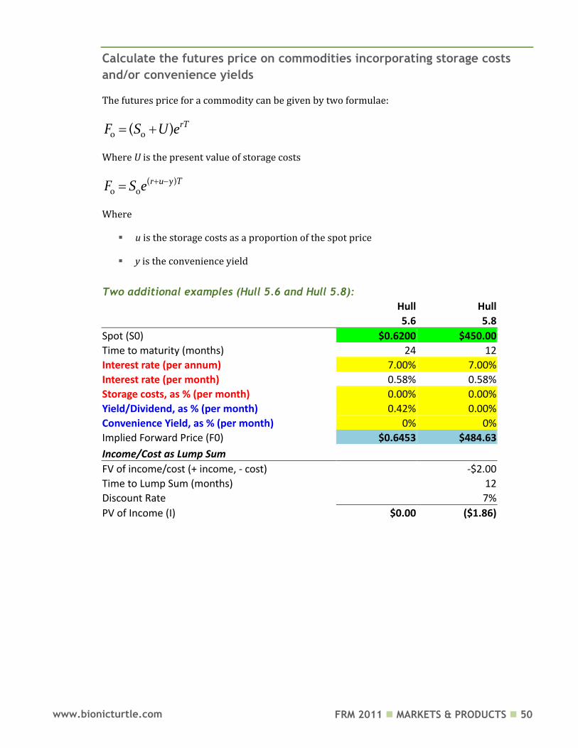
The futures price for a commodity can be given by two formulae:
0 0( ) rTF S U e
Where U is the present value of storage costs
( )0 0
r u y TF S e
Where
u is the storage costs as a proportion of the spot price
y is the convenience yield
Two additional examples (Hull 5.6 and Hull 5.8):
Hull Hull
5.6 5.8
Spot (S0) $0.6200 $450.00
Time to maturity (months) 24 12
Interest rate (per annum) 7.00% 7.00%
Interest rate (per month) 0.58% 0.58%
Storage costs, as % (per month) 0.00% 0.00%
Yield/Dividend, as % (per month) 0.42% 0.00%
Convenience Yield, as % (per month) 0% 0%
Implied Forward Price (F0) $0.6453 $484.63
Income/Cost as Lump Sum
FV of income/cost (+ income, - cost)
-$2.00
Time to Lump Sum (months)
12
Discount Rate
7%
PV of Income (I) $0.00 ($1.86)
FRM 2011 MARKETS & PRODUCTS 51 www.bionicturtle.com
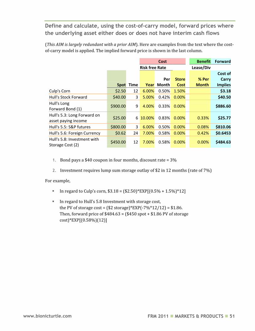
Define and calculate, using the cost‐of‐carry model, forward prices where
the underlying asset either does or does not have interim cash flows
(This AIM is largely redundant with a prior AIM). Here are examples from the text where the cost-
of-carry model is applied. The implied forward price is shown in the last column.
Cost Benefit Forward
Risk free Rate Lease/Div
Spot Time Year
Per Month
Store Cost
% Per Month
Cost of Carry
Implies
Culp's Corn $2.50 12
6.00% 0.50% 1.50%
$3.18
Hull's Stock Forward $40.00 3
5.00% 0.42% 0.00%
$40.50
Hull's Long Forward Bond (1)
$900.00 9
4.00% 0.33% 0.00%
$886.60
Hull's 5.3: Long Forward on asset paying income
$25.00 6 10.00% 0.83% 0.00%
0.33% $25.77
Hull's 5.5: S&P futures $800.00 3
6.00% 0.50% 0.00%
0.08% $810.06
Hull's 5.6: Foreign Currency $0.62 24
7.00% 0.58% 0.00%
0.42% $0.6453
Hull's 5.8: Investment with Storage Cost (2)
$450.00 12
7.00% 0.58% 0.00%
0.00% $484.63
1. Bond pays a $40 coupon in four months, discount rate = 3%
2. Investment requires lump sum storage outlay of $2 in 12 months (rate of 7%)
For example,
In regard to Culp’s corn, $3.18 = ($2.50)*EXP[(0.5% + 1.5%)*12]
In regard to Hull’s 5.8 Investment with storage cost,
the PV of storage cost = ($2 storage)*EXP(-7%*12/12) = $1.86.
Then, forward price of $484.63 = ($450 spot + $1.86 PV of storage
cost)*EXP[(0.58%)(12)]
FRM 2011 MARKETS & PRODUCTS 52 www.bionicturtle.com
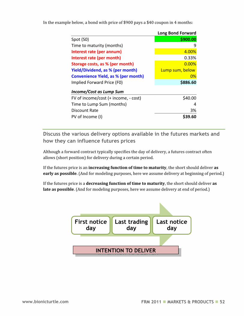
In the example below, a bond with price of $900 pays a $40 coupon in 4 months:
Long Bond Forward
Spot (S0) $900.00
Time to maturity (months) 9
Interest rate (per annum) 4.00%
Interest rate (per month) 0.33%
Storage costs, as % (per month) 0.00%
Yield/Dividend, as % (per month) Lump sum, below
Convenience Yield, as % (per month) 0%
Implied Forward Price (F0) $886.60
Income/Cost as Lump Sum
FV of income/cost (+ income, - cost) $40.00
Time to Lump Sum (months) 4
Discount Rate 3%
PV of Income (I) $39.60
Discuss the various delivery options available in the futures markets and
how they can influence futures prices
Although a forward contract typically specifies the day of delivery, a futures contract often
allows (short position) for delivery during a certain period.
If the futures price is an increasing function of time to maturity, the short should deliver as
early as possible. (And for modeling purposes, here we assume delivery at beginning of period.)
If the futures price is a decreasing function of time to maturity, the short should deliver as
late as possible. (And for modeling purposes, here we assume delivery at end of period.)
First notice day
Last trading day
Last notice day
INTENTION TO DELIVER
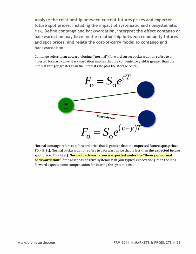
FRM 2011 MARKETS & PRODUCTS 53 www.bionicturtle.com
Analyze the relationship between current futures prices and expected
future spot prices, including the impact of systematic and nonsystematic
risk. Define contango and backwardation, interpret the effect contango or
backwardation may have on the relationship between commodity futures
and spot prices, and relate the cost‐of‐carry model to contango and
backwardation
Contango refers to an upward-sloping (“normal”) forward curve; backwardation refers to an
inverted forward curve. Backwardation implies that the convenience yield is greater than the
interest rate (or greater than the interest rate plus the storage costs):
Normal contango refers to a forward price that is greater than the expected future spot price:
F0 > E[St]. Normal backwardation refers to a forward price that is less than the expected future
spot price: F0 > E[St]. Normal backwardation is expected under the “theory of normal
backwardation:”if the asset has positive systemic risk (our typical expectation), then the long
forward expects some compensation for bearing the systemic risk.
Int
en
0 0
c y TF S e
0 0cTF S e
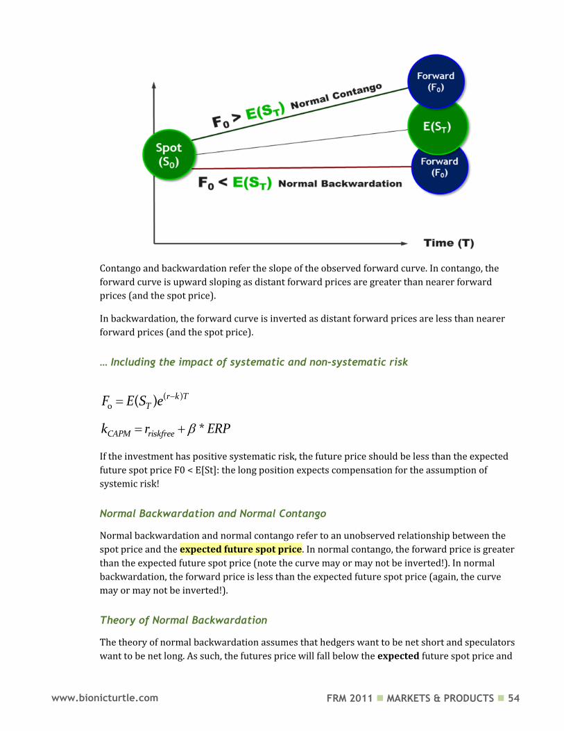
FRM 2011 MARKETS & PRODUCTS 54 www.bionicturtle.com
Contango and backwardation refer the slope of the observed forward curve. In contango, the
forward curve is upward sloping as distant forward prices are greater than nearer forward
prices (and the spot price).
In backwardation, the forward curve is inverted as distant forward prices are less than nearer
forward prices (and the spot price).
… Including the impact of systematic and non-systematic risk
( )0 ( ) r k T
TF E S e
*CAPM riskfreek r ERP
If the investment has positive systematic risk, the future price should be less than the expected
future spot price F0 < E[St]: the long position expects compensation for the assumption of
systemic risk!
Normal Backwardation and Normal Contango
Normal backwardation and normal contango refer to an unobserved relationship between the
spot price and the expected future spot price. In normal contango, the forward price is greater
than the expected future spot price (note the curve may or may not be inverted!). In normal
backwardation, the forward price is less than the expected future spot price (again, the curve
may or may not be inverted!).
Theory of Normal Backwardation
The theory of normal backwardation assumes that hedgers want to be net short and speculators
want to be net long. As such, the futures price will fall below the expected future spot price and
FRM 2011 MARKETS & PRODUCTS 55 www.bionicturtle.com
this is known as normal backwardation. If, instead, hedgers are net long and speculators are net
short, futures prices are greater than expected future spot prices and this is known as contango.
Do not confuse normal backwardation with backwardation. Normal backwardation is when the
when the futures price exceeds the expected future spot price. Backwardation is when the cash
price (i.e., today’s spot price) exceeds the futures price.
FRM 2011 MARKETS & PRODUCTS 56 www.bionicturtle.com
Hull, Chapter 6:
Interest Rate
Futures
In this chapter…
List the most commonly used day count conventions, identify the markets that each one is typically used in, and apply each to an interest calculation.
Convert from a discount rate to a price for a US Treasury bill. Differentiate between the clean and dirty price for a US Treasury bond;
calculate the accrued interest and dirty price on a US Treasury bond. Explain and calculate a US Treasury bond futures contract conversion factor. Calculate the cost of delivering a bond into a Treasury bond futures contract. Describe the impact of the level and shape of the yield curve on the cheapest‐
to‐deliver bond decision. Calculate the theoretical futures price for a Treasury bond futures contract. Calculate the final contract price on a Eurodollar futures contract. Describe and compute the Eurodollar futures contract convexity adjustment. Demonstrate how Eurodollar futures can be used to extend the LIBOR zero
curve. Calculate the duration‐based hedge ratio and describe a duration‐based hedging
strategy using interest rate futures. Explain the limitations of using a duration‐based hedging strategy.
List the most commonly used day count conventions, identify the markets
that each one is typically used in, and apply each to an interest
calculation
Day count conventions are important for computing accrued interest:
Actual/actual: U.S. Treasury bonds
30/360: U.S. corporate and municipal bonds
Actual/360: U.S. Treasury bills and other money market instruments
For example, if coupons pay on March 1st and September 1st, then actual/actual computes based
on actual/184 days while 30/360 would assume 180 days between coupons.
Money Market instruments include:
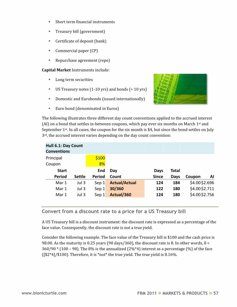
FRM 2011 MARKETS & PRODUCTS 57 www.bionicturtle.com
Short term financial instruments
Treasury bill (government)
Certificate of deposit (bank)
Commercial paper (CP)
Repurchase agreement (repo)
Capital Market Instruments include:
Long term securities
US Treasury notes (1-10 yrs) and bonds (> 10 yrs)
Domestic and Eurobonds (issued internationally)
Euro bond (denominated in Euros)
The following illustrates three different day count conventions applied to the accrued interest
(AI) on a bond that settles in-between coupons, which pay ever six months on March 1st and
September 1st. In all cases, the coupon for the six month is $4, but since the bond settles on July
3rd, the accrued interest varies depending on the day count convention:
Hull 6.1: Day Count Conventions
Principal
$100
Coupon
8%
Start
End Day Days Total
Period Settle Period
Count Since Days Coupon AI
Mar 1 Jul 3 Sep 1 Actual/Actual 124 184 $4.00 $2.696
Mar 1 Jul 3 Sep 1 30/360 122 180 $4.00 $2.711
Mar 1 Jul 3 Sep 1 Actual/360 124 180 $4.00 $2.756
Convert from a discount rate to a price for a US Treasury bill
A US Treasury bill is a discount instrument: the discount rate is expressed as a percentage of the
face value. Consequently, the discount rate is not a true yield.
Consider the following example. The face value of the Treasury bill is $100 and the cash price is
98.00. As the maturity is 0.25 years (90 days/360), the discount rate is 8. In other words, 8 =
360/90 * (100 – 98). The 8% is the annualized (2%*4) interest as a percentage (%) of the face
([$2*4]/$100). Therefore, it is *not* the true yield. The true yield is 8.16%.
FRM 2011 MARKETS & PRODUCTS 58 www.bionicturtle.com
Discount Rate for Treasury Bill Face
$100.00
n (days)
90 P (discount)(%) 8.0 = 8%
Y (cash price) 97.98
Solving for P
8.0 << Hull's formula: P = 360/n*(100-Y)
True Yield versus Discount Rate Discount rate(%) 8.00 Discount rate 8.00% True Yield (1) 8.16% True Yield (2) 8.16%
Differentiate between the clean and dirty price for a US Treasury bond;
calculate the accrued interest and dirty price on a US Treasury bond.
The clean price (i.e., the quoted price) does not reflect the cash price if interest has accrued. The
dirty price (i.e., the full price or the cash price) adds the accrued interest to the clean price. In
short: Cash Price = Quoted Price + Accrued Interest since last coupon date.
The illustration below computes the dirty price by adding the accrued interest (which, recall,
depends on the day count convention) to the quoted (clean) price.
Hull 6.1: Dirty Price of US Treasury Principal
$100
Coupon
11% Quoted Price (Clean) $95.50
Dirty
Start
End Day Days Total
(Full)
Period Settle Period Count Since Days Coupon AI Price
1/10/2010 3/5/2010 7/10/2010 Actual/Actual 54 181 $5.50 $1.641 $97.141
The flat price is also called the “clean price” or simply the “price”. The full price
is also called the “dirty price” or the “invoice price”.
When the accrued interest of a bond is zero (i.e., when the settlement date is a coupon payment
date) the flat and full prices of the bond are equal. When accrued interest is not zero, the amount
paid/received for a bond (i.e., its full price) should equal the present value of its cash flows.
If P is a bond’s flat price, and AI is the accrued interest, then the full price is the present value
(PV) which is given by:
P + AI = PV (future cash flows)
FRM 2011 MARKETS & PRODUCTS 59 www.bionicturtle.com
Where AI equals the accrued interest and is given by:
# of days from last coupon to settlementcoupon
# of days between couponsAI
To summarize, the full price of the bond equals the flat price plus accrued interest (if any).
The invoice price is the amount paid by the buyer and received by the seller; therefore, it is the
face amount multiplied by the full price. Here is another example:
Par $100.00
Last Coupon 1/1/2008
Yield 4%
Settlement 5/16/2008
Coupon (%) 8%
Next Coupon 7/1/2008
Coupon ($)
$4.00
Matures 7/1/2010
Years (from last coupon) 2.50
Present value "street method"
Price (at last coupon) $109.43
Period CF PV
1 $4.00 $3.98
w (days to next coupon) 45
2 $4.00 $3.90
days in coupon period 180
3 $4.00 $3.83
w periods 0.25
4 $4.00 $3.75
Accrued interest (AI) $3.00
5 $104.00 $95.61
Full Price (PV) $111.06
Full price $111.06
Full price (PV) is also the recent price (at last coupon) compounded forward: PV = ($109.43)[(1.02)^(1-w)]
Accrued interest (AI) $3.00 Clean price $108.06
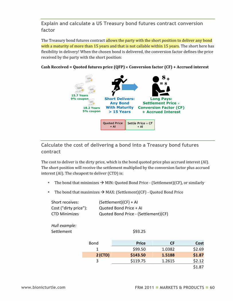
FRM 2011 MARKETS & PRODUCTS 60 www.bionicturtle.com
Explain and calculate a US Treasury bond futures contract conversion
factor
The Treasury bond futures contract allows the party with the short position to deliver any bond
with a maturity of more than 15 years and that is not callable within 15 years. The short here has
flexibility in delivery! When the chosen bond is delivered, the conversion factor defines the price
received by the party with the short position:
Cash Received = Quoted futures price (QFP) Conversion factor (CF) + Accrued interest
Calculate the cost of delivering a bond into a Treasury bond futures
contract
The cost to deliver is the dirty price, which is the bond quoted price plus accrued interest (AI).
The short position will receive the settlement multiplied by the conversion factor plus accrued
interest (AI). The cheapest to deliver (CTD) is:
The bond that minimizes MIN: Quoted Bond Price - (Settlement)(CF), or similarly
The bond that maximizes MAX: (Settlement)(CF) - Quoted Bond Price
Short receives: (Settlement)(CF) + AI
Cost ("dirty price"): Quoted Bond Price + AI
CTD Minimizes Quoted Bond Price - (Settlement)(CF)
Hull example:
Settlement $93.25
Bond Price CF Cost
1 $99.50 1.0382 $2.69
2 (CTD) $143.50 1.5188 $1.87
3 $119.75 1.2615 $2.12
$1.87
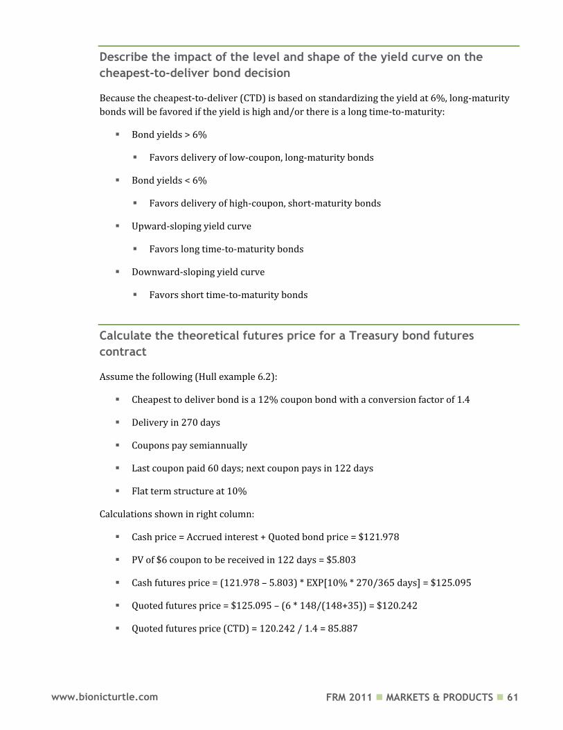
FRM 2011 MARKETS & PRODUCTS 61 www.bionicturtle.com
Describe the impact of the level and shape of the yield curve on the
cheapest‐to‐deliver bond decision
Because the cheapest-to-deliver (CTD) is based on standardizing the yield at 6%, long-maturity
bonds will be favored if the yield is high and/or there is a long time-to-maturity:
Bond yields > 6%
Favors delivery of low-coupon, long-maturity bonds
Bond yields < 6%
Favors delivery of high-coupon, short-maturity bonds
Upward-sloping yield curve
Favors long time-to-maturity bonds
Downward-sloping yield curve
Favors short time-to-maturity bonds
Calculate the theoretical futures price for a Treasury bond futures
contract
Assume the following (Hull example 6.2):
Cheapest to deliver bond is a 12% coupon bond with a conversion factor of 1.4
Delivery in 270 days
Coupons pay semiannually
Last coupon paid 60 days; next coupon pays in 122 days
Flat term structure at 10%
Calculations shown in right column:
Cash price = Accrued interest + Quoted bond price = $121.978
PV of $6 coupon to be received in 122 days = $5.803
Cash futures price = (121.978 – 5.803) * EXP[10% * 270/365 days] = $125.095
Quoted futures price = $125.095 – (6 * 148/(148+35)) = $120.242
Quoted futures price (CTD) = 120.242 / 1.4 = 85.887
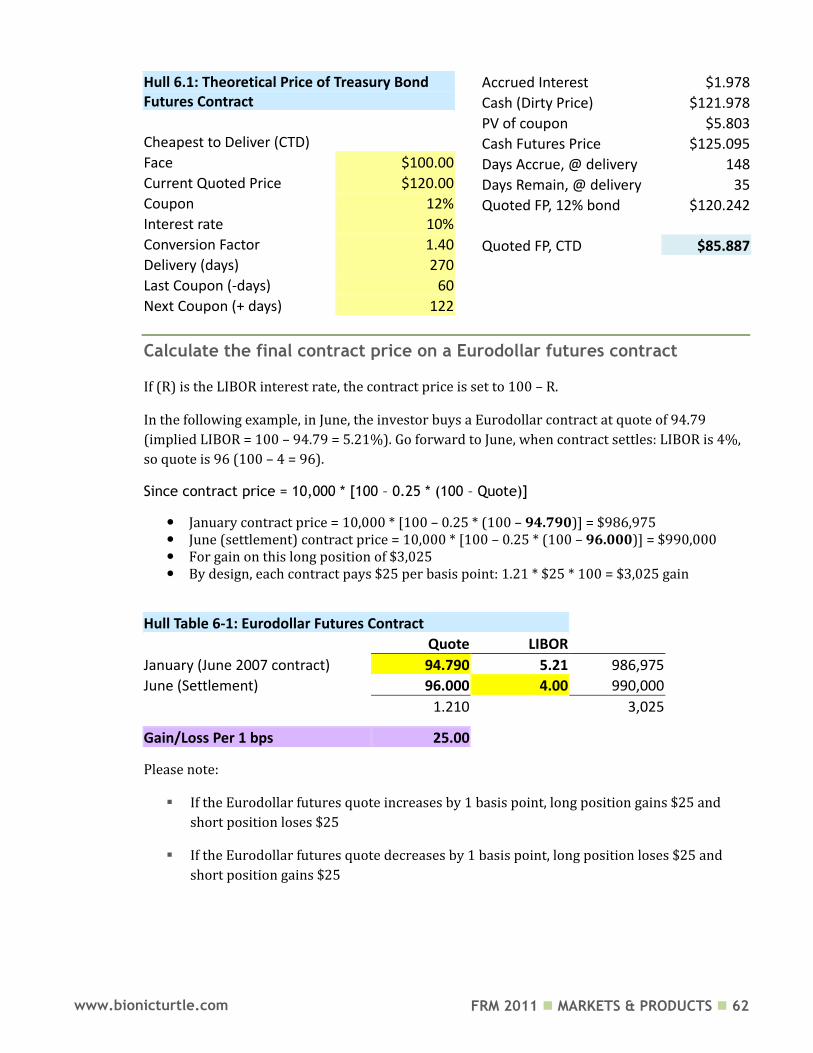
FRM 2011 MARKETS & PRODUCTS 62 www.bionicturtle.com
Calculate the final contract price on a Eurodollar futures contract
If (R) is the LIBOR interest rate, the contract price is set to 100 – R.
In the following example, in June, the investor buys a Eurodollar contract at quote of 94.79
(implied LIBOR = 100 – 94.79 = 5.21%). Go forward to June, when contract settles: LIBOR is 4%,
so quote is 96 (100 – 4 = 96).
Since contract price = 10,000 * [100 – 0.25 * (100 – Quote)]
January contract price = 10,000 * [100 – 0.25 * (100 – 94.790)] = $986,975 June (settlement) contract price = 10,000 * [100 – 0.25 * (100 – 96.000)] = $990,000 For gain on this long position of $3,025 By design, each contract pays $25 per basis point: 1.21 * $25 * 100 = $3,025 gain
Hull Table 6-1: Eurodollar Futures Contract
Quote LIBOR
January (June 2007 contract) 94.790 5.21 986,975
June (Settlement) 96.000 4.00 990,000
1.210
3,025
Gain/Loss Per 1 bps 25.00
Please note:
If the Eurodollar futures quote increases by 1 basis point, long position gains $25 and
short position loses $25
If the Eurodollar futures quote decreases by 1 basis point, long position loses $25 and
short position gains $25
Hull 6.1: Theoretical Price of Treasury Bond Futures Contract
Cheapest to Deliver (CTD)
Face
$100.00
Current Quoted Price $120.00
Coupon
12%
Interest rate 10%
Conversion Factor 1.40
Delivery (days) 270
Last Coupon (-days) 60
Next Coupon (+ days) 122
Accrued Interest $1.978
Cash (Dirty Price) $121.978
PV of coupon $5.803
Cash Futures Price $125.095
Days Accrue, @ delivery 148
Days Remain, @ delivery 35
Quoted FP, 12% bond $120.242
Quoted FP, CTD $85.887
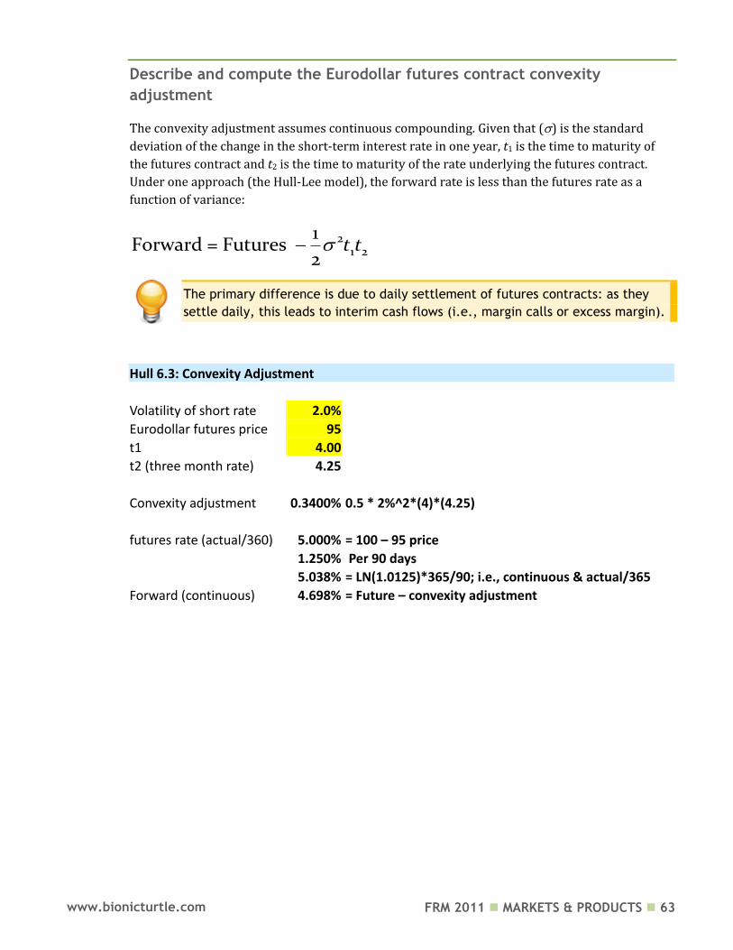
FRM 2011 MARKETS & PRODUCTS 63 www.bionicturtle.com
Describe and compute the Eurodollar futures contract convexity
adjustment
The convexity adjustment assumes continuous compounding. Given that () is the standard
deviation of the change in the short-term interest rate in one year, t1 is the time to maturity of
the futures contract and t2 is the time to maturity of the rate underlying the futures contract.
Under one approach (the Hull-Lee model), the forward rate is less than the futures rate as a
function of variance:
21 2
1Forward = Futures
2t t
The primary difference is due to daily settlement of futures contracts: as they
settle daily, this leads to interim cash flows (i.e., margin calls or excess margin).
Hull 6.3: Convexity Adjustment
Volatility of short rate 2.0%
Eurodollar futures price 95
t1
4.00
t2 (three month rate) 4.25
Convexity adjustment 0.3400% 0.5 * 2%^2*(4)*(4.25)
futures rate (actual/360) 5.000% = 100 – 95 price
1.250% Per 90 days
5.038% = LN(1.0125)*365/90; i.e., continuous & actual/365
Forward (continuous) 4.698% = Future – convexity adjustment
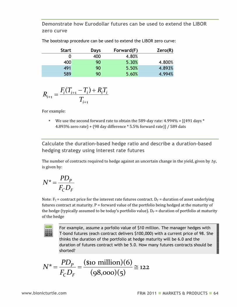
FRM 2011 MARKETS & PRODUCTS 64 www.bionicturtle.com
Demonstrate how Eurodollar futures can be used to extend the LIBOR
zero curve
The bootstrap procedure can be used to extend the LIBOR zero curve:
Start Days Forward(F) Zero(R)
0 400 4.80%
400 90 5.30% 4.800%
491 90 5.50% 4.893%
589 90 5.60% 4.994%
11
1
( )i i i i ii
i
F T T RTR
T
For example:
We use the second forward rate to obtain the 589-day rate: 4.994% = [(491 days *
4.893% zero rate) + (98 day difference * 5.5% forward rate)] / 589 dats
Calculate the duration‐based hedge ratio and describe a duration‐based
hedging strategy using interest rate futures
The number of contracts required to hedge against an uncertain change in the yield, given by y,
is given by:
* P
C F
PDN
F D
Note: FC = contract price for the interest rate futures contract. DF = duration of asset underlying
futures contract at maturity. P = forward value of the portfolio being hedged at the maturity of
the hedge (typically assumed to be today’s portfolio value). DP = duration of portfolio at maturity
of the hedge
For example, assume a porfolio value of $10 million. The manager hedges with
T-bond futures (each contract delivers $100,000) with a current price of 98. She
thinks the duration of the portfolio at hedge maturity will be 6.0 and the
duration of futures contract with be 5.0. How many futures contracts should be
shorted?
($10 million)(6)* 122
(98,000)(5)P
C F
PDN
F D
FRM 2011 MARKETS & PRODUCTS 65 www.bionicturtle.com
Explain the limitations of using a duration‐based hedging strategy
Portfolio immunization or duration matching is when a bank or fund matches the average
duration of assets with the average duration of liabilities.
Duration matching protects or “immunizes” against small, parallel shifts in the yield (interest
rate) curve. The limitation is that it does not protect against nonparallel shifts. The two most
common nonparallel shifts are:
A twist in the slope of the yield curve, or
A change in curvature
Distinguish between treasury rates, London Interbank Offered Rate (LIBOR) and repo rates
Treasury rates are applicable when a government borrows its own currency. Because we
assume the government will not default (e.g., U.S. Treasuries), this is called a risk-free rate.
London Interbank Offered Rate (LIBOR) is the going rate at which large, international banks
lend each other. There is only a small (even tiny) risk of default, but LIBOR rates are not entirely
risk-free and therefore the risk is slightly higher than treasury rates. Because the rate is between
large banks, it is considered a wholesale rate.
The LIBOR rate is not available to all financial institutions. In general, a bank
can borrow at LIBOR if they are AA-rated or better.
A repo rate is the implied rate on a repurchase agreement (i.e., a dealer sells securities today
with the promise to buy them back in the future). An overnight repo is renegotiated each date,
while longer term arrangements are known as term repos.
Calculate simple, semiannual, monthly, daily, and continuously compounded rates given a discount factor or market interest rate for a specified interval (this is useful because it arises again in fixed income)
Use this notation:
Initial investment = A
Interest rate = R per year (per annum)
Number of years = n
To illustrate with examples, we will assume:
An initial investment of (A=$100),
An annual interest rate of 6% per year (R=0.06), and
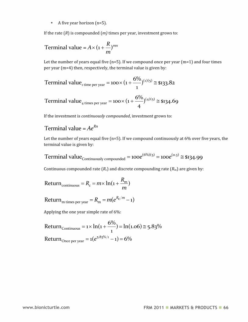
FRM 2011 MARKETS & PRODUCTS 66 www.bionicturtle.com
A five year horizon (n=5).
If the rate (R) is compounded (m) times per year, investment grows to:
Terminal value = (1 )mnRA
m
Let the number of years equal five (n=5). If we compound once per year (m=1) and four times
per year (m=4) then, respectively, the terminal value is given by:
(1)(5)1 time per year
6%Terminal value 100 (1 ) $133.82
1
(4)(5)4 times per year
6%Terminal value 100 (1 ) $134.69
4
If the investment is continuously compounded, investment grows to:
Terminal value = RnAe
Let the number of years equal five (n=5). If we compound continuously at 6% over five years, the
terminal value is given by:
(6%)(5) (0.3)Continuously compoundedTerminal value 100 100 $134.99e e
Continuous compounded rate (Rc) and discrete compounding rate (Rm) are given by:
mcontinuous cReturn ln(1 )
RR m
m
cm times per year mReturn ( 1)R mR m e
Applying the one year simple rate of 6%:
Continuous
5.83% 1Once per year
6%Return 1 ln(1 ) ln(1.06) 5.83%
1
Return 1( 1) 6%e
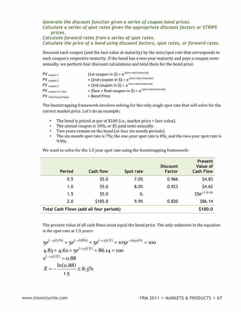
FRM 2011 MARKETS & PRODUCTS 67 www.bionicturtle.com
Generate the discount function given a series of coupon bond prices. Calculate a series of spot rates given the appropriate discount factors or STRIPS
prices. Calculate forward rates from a series of spot rates. Calculate the price of a bond using discount factors, spot rates, or forward rates.
Discount each coupon (and the face value at maturity) by the zero/spot rate that corresponds to
each coupon’s respective maturity. If the bond has a two-year maturity and pays a coupon semi-
annually, we perform four discount calculations and total them for the bond price:
PV coupon 1 (1st coupon in $) e-(zero rate) (maturity) PV coupon 2 + (2nd coupon in $) e-(zero rate) (maturity) PV coupon 3 + (3rd coupon in $) e-(zero rate) (maturity) PV coupon 4 + Face + (face + final coupon in $) e-(zero rate) (maturity) PV Total Future Flows = Bond Price
The bootstrapping framework involves solving for the only single spot rate that will solve for the
correct market price. Let’s do an example:
The bond is priced at par of $100 (i.e., market price = face value). The annual coupon is 10%, or $5 paid semi-annually. Two years remain on the bond (or four six month periods). The six-month spot rate is 7%; the one-year spot rate is 8%; and the two-year spot rate is
9.9%.
We want to solve for the 1.5 year spot rate using the bootstrapping framework:
Period
Cash flow
Spot rate
Discount
Factor
Present Value of
Cash Flow
0.5 $5.0 7.0% 0.966 $4.83
1.0 $5.0 8.0% 0.923 $4.62
1.5 $5.0 X? $5e(-1.5) (X)
2.0 $105.0 9.9% 0.820 $86.14
Total Cash Flows (add all four periods) $100.0
The present value of all cash flows must equal the bond price. The only unknown in the equation
is the spot rate at 1.5 years:
( .5)(7%) ( 1)(8%) ( 1.5)( ) 2(9.9%)
( 1.5)( )
( 1.5)( )
5 5 5 105 100
4.83 4.62 5 86.14 100
0.88
ln(0.88)8.3%
1.5
X
X
X
e e e e
e
e
X
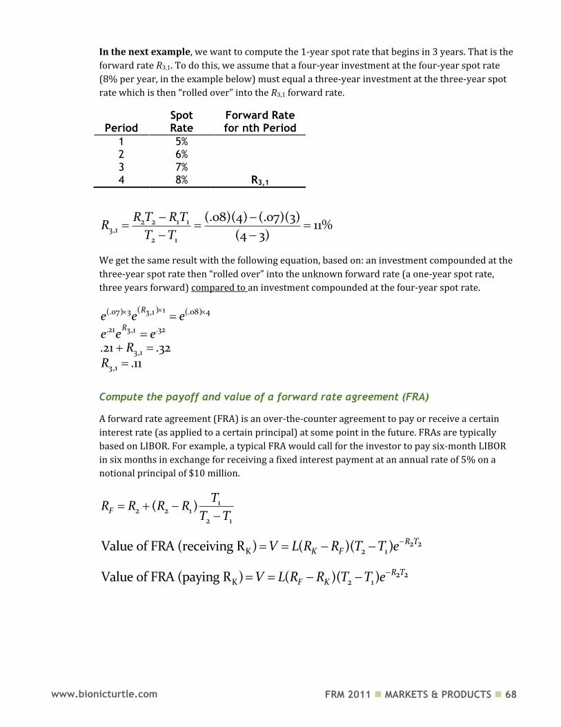
FRM 2011 MARKETS & PRODUCTS 68 www.bionicturtle.com
In the next example, we want to compute the 1-year spot rate that begins in 3 years. That is the
forward rate R3,1. To do this, we assume that a four-year investment at the four-year spot rate
(8% per year, in the example below) must equal a three-year investment at the three-year spot
rate which is then “rolled over” into the R3,1 forward rate.
Period
Spot Rate
Forward Rate for nth Period
1 5% 2 6% 3 7% 4 8% R3,1
2 2 1 13,1
2 1
(.08)(4) (.07)(3)11%
(4 3)
R T RTR
T T
We get the same result with the following equation, based on: an investment compounded at the
three-year spot rate then “rolled over” into the unknown forward rate (a one-year spot rate,
three years forward) compared to an investment compounded at the four-year spot rate.
( ) 1(.07) 3 (.08) 43,1
.21 .323,1
3,1
3,1
.21 .32.11
R
Re e e
e e eR
R
Compute the payoff and value of a forward rate agreement (FRA)
A forward rate agreement (FRA) is an over-the-counter agreement to pay or receive a certain
interest rate (as applied to a certain principal) at some point in the future. FRAs are typically
based on LIBOR. For example, a typical FRA would call for the investor to pay six-month LIBOR
in six months in exchange for receiving a fixed interest payment at an annual rate of 5% on a
notional principal of $10 million.
12 2 1
2 1
( )F
TR R R R
T T
2 2K 2 1Value of FRA (receiving R ) ( )( ) R T
K FV L R R T T e
2 2K 2 1Value of FRA (paying R ) ( )( ) R T
F KV L R R T T e
FRM 2011 MARKETS & PRODUCTS 69 www.bionicturtle.com
FRA Notation
There are two notations used for FRA. Consider an FRA entered into on Jan 1st. The FRA will
expire in six months, at which time ACME Corp. will pay the 6-month LIBOR interest rate and
receive a fixed rate of 5% (the annualized rate, but only six months’ worth of interest will be
collected).
The FRA is entered on Jan 1st; the FRA expires on June 30th and the net payment is determined
at that time based on the LIBOR rate at that time. If for example, LIBOR happens to be 5%, there
is no net settlement. If the 6-month LIBOR, in six months’ time, happens to be 4%, then ACME
Corp. will receive a payment as follows:
Receive-fixed: 5% x ½ Year x Notional Principal ($)
Pay-floating:(-) 4% x ½ Year x Notional Principal ($)
= +1% x ½ Year x Notional Principal ($)
The first notation method to describe this swap is given by:
6 × 12 5%
[Term to Expire, Months] × [Term to End of Period Covered by FRA] [Fixed Rate]
The second notation method to describe this (same) swap:
FRA6,12 = 5%
Explain the following theories of the term structure: expectations theory, market segmentation, and the liquidity preference theory
Expectations theory: Long-term rates reflect expected future short-term rates. Technically, this
says forward rates correspond to future zero rates.
Segmentation theory: Supply and demand determine each segment; this implies no intrinsic
relationship between short, medium and long rates.
Liquidity preference theory: Investors prefer shorter time periods and borrowers prefer
longer time periods. This would explain upper sloping yield curves, where forward rates tend to
exceed future zero rates.
Calculate the duration and modified duration of a bond (covered in fixed income) Duration of a Bond
The duration of a bond (D) is given by a formula that says “the percentage change of a bond’s
price (B) is a function of its duration (D) and the change in the yield:”
FRM 2011 MARKETS & PRODUCTS 70 www.bionicturtle.com
1
BD y
BB
DB y
If we recast the same equation with deltas, we get: the duration multiplied by the change in yield
(D
B
D yB
And solving this equation for the duration (D) gives us:
1B
DB y
This should be familiar. Assume a 50 basis point change produces a $50 price change to a bond
that is currently priced at $950. The duration is given by:
50 1
10.53950 (0.005)
D
Duration is the percentage change (%) in bond price for a 1% (100 basis points)
change in yield. Our duration of about 10.5 above implies that a 1% increase in
yield will produce a -10.5% decrease in price. So, a 50 basis point decline will
produce a 5.25% (10.5%
Modified Duration of a Bond (D*)
*1
DD
y m
Continuing the example, for a given a yield (y), the modified duration is given by:
10.53
*1 2
Dy
This is identical to duration from the Section II.1 readings. Hull’s “duration” is
Macaulay duration (which tends to be expressed as an average number of years)
and the “modified duration” formula above is identical to the modified duration
from earlier readings.
FRM 2011 MARKETS & PRODUCTS 71 www.bionicturtle.com
Duration-Based Hedging
Duration measures the change in value of the portfolio given a change in interest rates. But
duration assumes very small parallel shifts in the yield curve. Therefore, it does not handle:
Nonparallel shifts in the yield curve, and/or
Large parallel shifts in the yield curve
In regard to large parallel shifts, the reason is because the yield curve is not linear (whereas the
duration metric assumes linearity). The curvature of the yield curve can be addressed by
incorporating convexity
FRM 2011 MARKETS & PRODUCTS 72 www.bionicturtle.com
Hull, Chapter 7:
Swaps
In this chapter…
Explain the mechanics of a plain vanilla interest rate swap and compute its cash flows.
Explain how a plain vanilla interest rate swap can be used to transform an asset or a liability and calculate the resulting cash flows.
Explain the role of financial intermediaries in the swaps market. Describe the role of the confirmation in a swap transaction. Describe the comparative advantage argument for the existence of interest rate
swaps and discuss some of the criticisms of this argument. Explain how the discount rates in a plain vanilla interest rate swap are
computed. Value a plain vanilla interest rate swap based on two simultaneous bond
positions. Value a plain vanilla interest rate swap from a sequence of forward rate
agreements (FRAs). Explain the mechanics of a currency swap and compute its cash flows. Describe the comparative advantage argument for the existence of currency
swaps. Explain how a currency swap can be used to transform an asset or liability and
calculate the resulting cash flows. Value a currency swap based on two simultaneous bond positions. Value a currency swap based on a sequence of FRAs. Discuss the role of credit risk inherent in an existing swap position. List and define other types of swaps, including commodity, volatility and exotic
swaps.
Explain the mechanics of a plain vanilla interest rate swap and compute
its cash flows
In a plain-vanilla interest-rate swap, one company agrees to pay a fixed interest rate and receive
a variable interest rate (i.e., “pay-fixed and receive-floating”) and the other company (a.k.a., the
counterparty) agrees to pay a variable rate and receive a fixed interest rate (i.e., “pay-floating
and receive-fixed”).
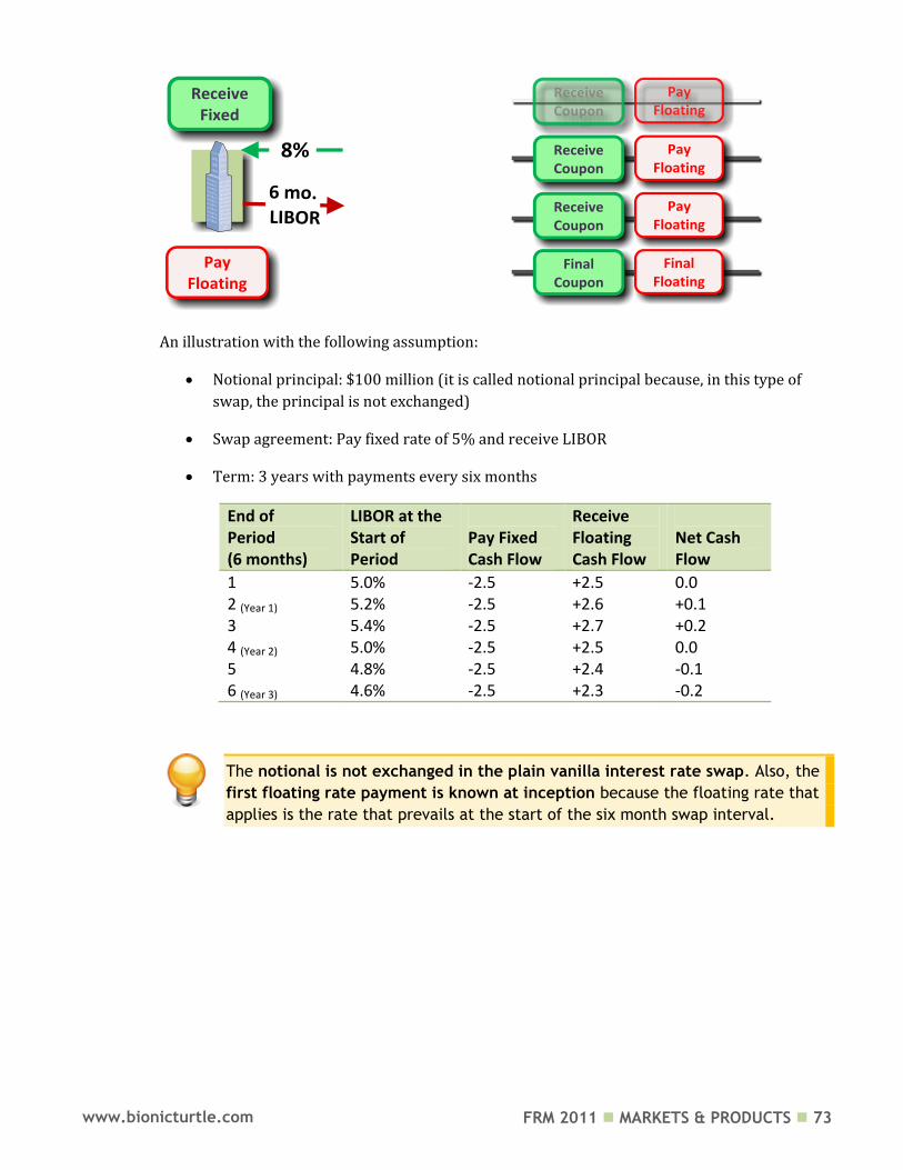
FRM 2011 MARKETS & PRODUCTS 73 www.bionicturtle.com
An illustration with the following assumption:
Notional principal: $100 million (it is called notional principal because, in this type of
swap, the principal is not exchanged)
Swap agreement: Pay fixed rate of 5% and receive LIBOR
Term: 3 years with payments every six months
End of Period (6 months)
LIBOR at the Start of Period
Pay Fixed Cash Flow
Receive Floating Cash Flow
Net Cash Flow
1 5.0% -2.5 +2.5 0.0 2 (Year 1) 5.2% -2.5 +2.6 +0.1 3 5.4% -2.5 +2.7 +0.2 4 (Year 2) 5.0% -2.5 +2.5 0.0 5 4.8% -2.5 +2.4 -0.1 6 (Year 3) 4.6% -2.5 +2.3 -0.2
The notional is not exchanged in the plain vanilla interest rate swap. Also, the
first floating rate payment is known at inception because the floating rate that
applies is the rate that prevails at the start of the six month swap interval.
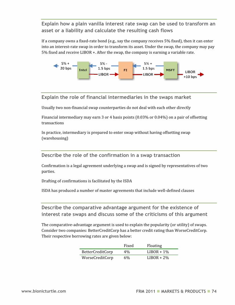
FRM 2011 MARKETS & PRODUCTS 74 www.bionicturtle.com
Explain how a plain vanilla interest rate swap can be used to transform an
asset or a liability and calculate the resulting cash flows
If a company owns a fixed-rate bond (e.g., say the company receives 5% fixed), then it can enter
into an interest-rate swap in order to transform its asset. Under the swap, the company may pay
5% fixed and receive LIBOR +. After the swap, the company is earning a variable rate.
Explain the role of financial intermediaries in the swaps market
Usually two non-financial swap counterparties do not deal with each other directly
Financial intermediary may earn 3 or 4 basis points (0.03% or 0.04%) on a pair of offsetting
transactions
In practice, intermediary is prepared to enter swap without having offsetting swap
(warehousing)
Describe the role of the confirmation in a swap transaction
Confirmation is a legal agreement underlying a swap and is signed by representatives of two
parties.
Drafting of confirmations is facilitated by the ISDA
ISDA has produced a number of master agreements that include well-defined clauses
Describe the comparative advantage argument for the existence of
interest rate swaps and discuss some of the criticisms of this argument
The comparative-advantage argument is used to explain the popularity (or utility) of swaps.
Consider two companies: BetterCreditCorp has a better credit rating than WorseCreditCorp.
Their respective borrowing rates are given below:
Fixed Floating
BetterCreditCorp 4% LIBOR + 1%
WorseCreditCorp 6% LIBOR + 2%
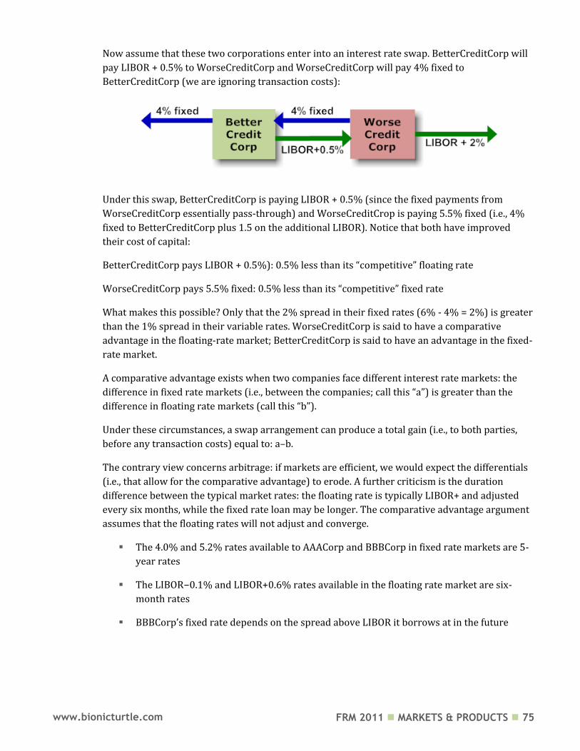
FRM 2011 MARKETS & PRODUCTS 75 www.bionicturtle.com
Now assume that these two corporations enter into an interest rate swap. BetterCreditCorp will
pay LIBOR + 0.5% to WorseCreditCorp and WorseCreditCorp will pay 4% fixed to
BetterCreditCorp (we are ignoring transaction costs):
Under this swap, BetterCreditCorp is paying LIBOR + 0.5% (since the fixed payments from
WorseCreditCorp essentially pass-through) and WorseCreditCrop is paying 5.5% fixed (i.e., 4%
fixed to BetterCreditCorp plus 1.5 on the additional LIBOR). Notice that both have improved
their cost of capital:
BetterCreditCorp pays LIBOR + 0.5%): 0.5% less than its “competitive” floating rate
WorseCreditCorp pays 5.5% fixed: 0.5% less than its “competitive” fixed rate
What makes this possible? Only that the 2% spread in their fixed rates (6% - 4% = 2%) is greater
than the 1% spread in their variable rates. WorseCreditCorp is said to have a comparative
advantage in the floating-rate market; BetterCreditCorp is said to have an advantage in the fixed-
rate market.
A comparative advantage exists when two companies face different interest rate markets: the
difference in fixed rate markets (i.e., between the companies; call this “a”) is greater than the
difference in floating rate markets (call this “b”).
Under these circumstances, a swap arrangement can produce a total gain (i.e., to both parties,
before any transaction costs) equal to: a–b.
The contrary view concerns arbitrage: if markets are efficient, we would expect the differentials
(i.e., that allow for the comparative advantage) to erode. A further criticism is the duration
difference between the typical market rates: the floating rate is typically LIBOR+ and adjusted
every six months, while the fixed rate loan may be longer. The comparative advantage argument
assumes that the floating rates will not adjust and converge.
The 4.0% and 5.2% rates available to AAACorp and BBBCorp in fixed rate markets are 5-
year rates
The LIBOR−0.1% and LIBOR+0.6% rates available in the floating rate market are six-
month rates
BBBCorp’s fixed rate depends on the spread above LIBOR it borrows at in the future
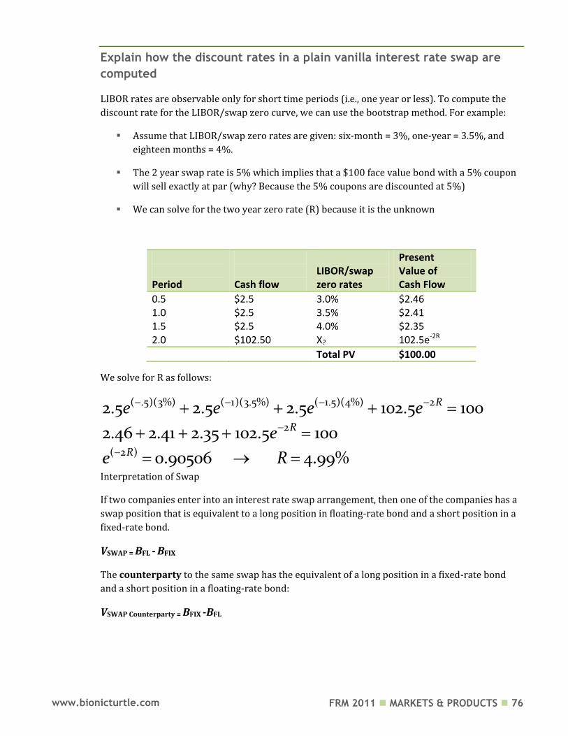
FRM 2011 MARKETS & PRODUCTS 76 www.bionicturtle.com
Explain how the discount rates in a plain vanilla interest rate swap are
computed
LIBOR rates are observable only for short time periods (i.e., one year or less). To compute the
discount rate for the LIBOR/swap zero curve, we can use the bootstrap method. For example:
Assume that LIBOR/swap zero rates are given: six-month = 3%, one-year = 3.5%, and
eighteen months = 4%.
The 2 year swap rate is 5% which implies that a $100 face value bond with a 5% coupon
will sell exactly at par (why? Because the 5% coupons are discounted at 5%)
We can solve for the two year zero rate (R) because it is the unknown
Period
Cash flow
LIBOR/swap zero rates
Present Value of Cash Flow
0.5 $2.5 3.0% $2.46 1.0 $2.5 3.5% $2.41 1.5 $2.5 4.0% $2.35 2.0 $102.50 X? 102.5e-2R
Total PV $100.00
We solve for R as follows:
( .5)(3%) ( 1)(3.5%) ( 1.5)(4%) 2
2
( 2 )
2.5 2.5 2.5 102.5 100
2.46 2.41 2.35 102.5 100
0.90506 4.99%
R
R
R
e e e e
e
e R
Interpretation of Swap
If two companies enter into an interest rate swap arrangement, then one of the companies has a
swap position that is equivalent to a long position in floating-rate bond and a short position in a
fixed-rate bond.
VSWAP = BFL - BFIX
The counterparty to the same swap has the equivalent of a long position in a fixed-rate bond
and a short position in a floating-rate bond:
VSWAP Counterparty = BFIX -BFL
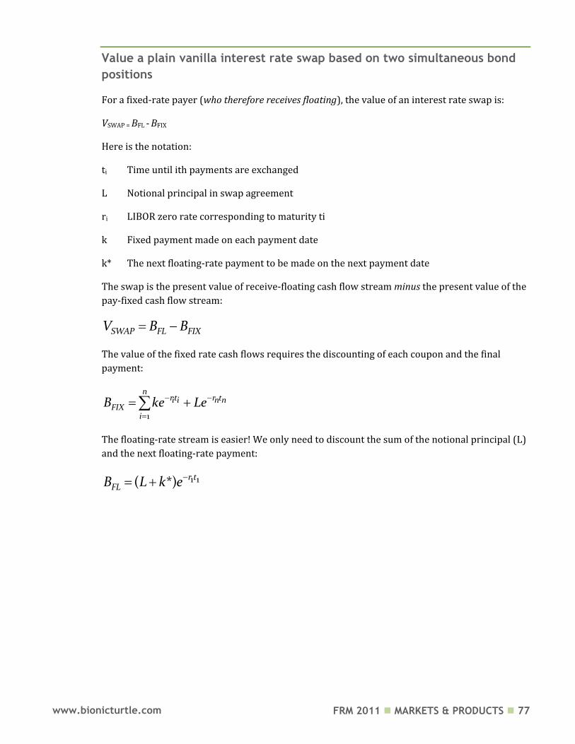
FRM 2011 MARKETS & PRODUCTS 77 www.bionicturtle.com
Value a plain vanilla interest rate swap based on two simultaneous bond
positions
For a fixed-rate payer (who therefore receives floating), the value of an interest rate swap is:
VSWAP = BFL - BFIX
Here is the notation:
ti Time until ith payments are exchanged
L Notional principal in swap agreement
ri LIBOR zero rate corresponding to maturity ti
k Fixed payment made on each payment date
k* The next floating-rate payment to be made on the next payment date
The swap is the present value of receive-floating cash flow stream minus the present value of the
pay-fixed cash flow stream:
SWAP FL FIXV B B
The value of the fixed rate cash flows requires the discounting of each coupon and the final
payment:
1
nrt r ti i n n
FIXi
B ke Le
The floating-rate stream is easier! We only need to discount the sum of the notional principal (L)
and the next floating-rate payment:
1 1( *) r tFLB L k e
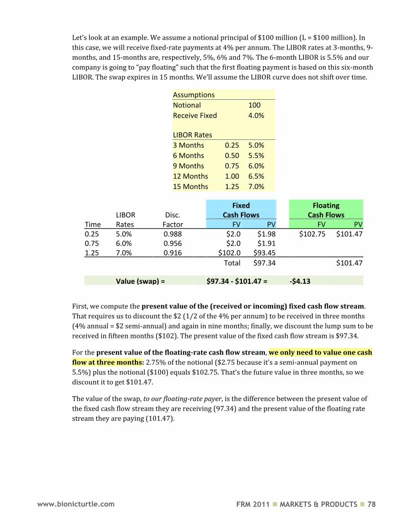
FRM 2011 MARKETS & PRODUCTS 78 www.bionicturtle.com
Let’s look at an example. We assume a notional principal of $100 million (L = $100 million). In
this case, we will receive fixed-rate payments at 4% per annum. The LIBOR rates at 3-months, 9-
months, and 15-months are, respectively, 5%, 6% and 7%. The 6-month LIBOR is 5.5% and our
company is going to “pay floating” such that the first floating payment is based on this six-month
LIBOR. The swap expires in 15 months. We’ll assume the LIBOR curve does not shift over time.
Assumptions
Notional 100
Receive Fixed 4.0%
LIBOR Rates
3 Months 0.25 5.0%
6 Months 0.50 5.5%
9 Months 0.75 6.0%
12 Months 1.00 6.5%
15 Months 1.25 7.0%
Fixed
Floating
LIBOR Disc.
Cash Flows
Cash Flows
Time Rates Factor FV PV FV PV 0.25 5.0% 0.988
$2.0 $1.98
$102.75 $101.47
0.75 6.0% 0.956
$2.0 $1.91
1.25 7.0% 0.916
$102.0 $93.45
Total $97.34 $101.47
Value (swap) = $97.34 - $101.47 = -$4.13
First, we compute the present value of the (received or incoming) fixed cash flow stream.
That requires us to discount the $2 (1/2 of the 4% per annum) to be received in three months
(4% annual = $2 semi-annual) and again in nine months; finally, we discount the lump sum to be
received in fifteen months ($102). The present value of the fixed cash flow stream is $97.34.
For the present value of the floating-rate cash flow stream, we only need to value one cash
flow at three months: 2.75% of the notional ($2.75 because it’s a semi-annual payment on
5.5%) plus the notional ($100) equals $102.75. That’s the future value in three months, so we
discount it to get $101.47.
The value of the swap, to our floating-rate payer, is the difference between the present value of
the fixed cash flow stream they are receiving (97.34) and the present value of the floating rate
stream they are paying (101.47).
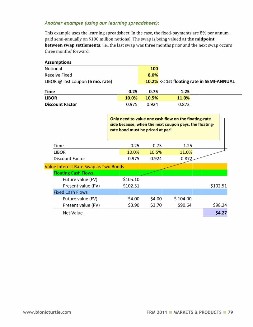
FRM 2011 MARKETS & PRODUCTS 79 www.bionicturtle.com
Another example (using our learning spreadsheet):
This example uses the learning spreadsheet. In the case, the fixed-payments are 8% per annum,
paid semi-annually on $100 million notional. The swap is being valued at the midpoint
between swap settlements; i.e., the last swap was three months prior and the next swap occurs
three months’ forward.
Assumptions Notional
100
Receive Fixed
8.0% LIBOR @ last coupon (6 mo. rate)
10.2% << 1st floating rate in SEMI-ANNUAL
Time 0.25 0.75 1.25
LIBOR 10.0% 10.5% 11.0% Discount Factor 0.975 0.924 0.872
Time 0.25 0.75 1.25
LIBOR 10.0% 10.5% 11.0%
Discount Factor 0.975 0.924 0.872
Value Interest Rate Swap as Two Bonds
Floating Cash Flows
Future value (FV) $105.10
Present value (PV) $102.51
$102.51
Fixed Cash Flows
Future value (FV) $4.00 $4.00 $ 104.00
Present value (PV) $3.90 $3.70 $90.64
$98.24
Net Value $4.27
Only need to value one cash flow on the floating-rate side because, when the next coupon pays, the floating-rate bond must be priced at par!
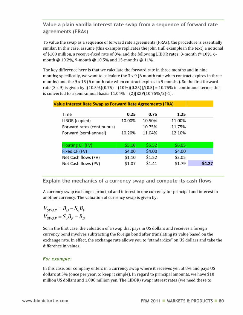
FRM 2011 MARKETS & PRODUCTS 80 www.bionicturtle.com
Value a plain vanilla interest rate swap from a sequence of forward rate
agreements (FRAs)
To value the swap as a sequence of forward rate agreements (FRAs), the procedure is essentially
similar. In this case, assume (this example replicates the John Hull example in the text) a notional
of $100 million, a receive-fixed rate of 8%, and the following LIBOR rates: 3-month @ 10%, 6-
month @ 10.2%, 9-month @ 10.5% and 15-months @ 11%.
The key difference here is that we calculate the forward rate in three months and in nine
months; specifically, we want to calculate the 3 x 9 (6 month rate when contract expires in three
months) and the 9 x 15 (6 month rate when contract expires in 9 months). So the first forward
rate (3 x 9) is given by [(10.5%)(0.75) – (10%)(0.25)]/(0.5) = 10.75% in continuous terms; this
is converted to a semi-annual basis: 11.04% = (2)[EXP(10.75%/2)-1].
Value Interest Rate Swap as Forward Rate Agreements (FRA) Time 0.25 0.75 1.25 LIBOR (copied) 10.00% 10.50% 11.00%
Forward rates (continuous)
10.75% 11.75%
Forward (semi-annual) 10.20% 11.04% 12.10%
Floating CF (FV) $5.10 $5.52 $6.05
Fixed CF (FV) $4.00 $4.00 $4.00
Net Cash flows (FV) $1.10 $1.52 $2.05
Net Cash flows (PV) $1.07 $1.41 $1.79
$4.27
Explain the mechanics of a currency swap and compute its cash flows
A currency swap exchanges principal and interest in one currency for principal and interest in
another currency. The valuation of currency swap is given by:
0
0
SWAP D F
SWAP F D
V B S B
V S B B
So, in the first case, the valuation of a swap that pays in US dollars and receives a foreign
currency bond involves subtracting the foreign bond after translating its value based on the
exchange rate. In effect, the exchange rate allows you to “standardize” on US dollars and take the
difference in values.
For example:
In this case, our company enters in a currency swap where it receives yen at 8% and pays US
dollars at 5% (once per year, to keep it simple). In regard to principal amounts, we have $10
million US dollars and 1,000 million yen. The LIBOR/swap interest rates (we need these to
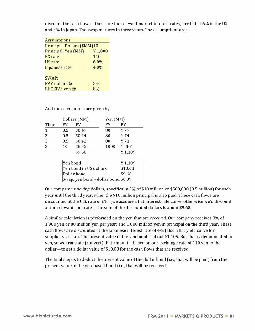
FRM 2011 MARKETS & PRODUCTS 81 www.bionicturtle.com
discount the cash flows – these are the relevant market interest rates) are flat at 6% in the US
and 4% in Japan. The swap matures in three years. The assumptions are:
Assumptions Principal, Dollars ($MM) 10 Principal, Yen (MM) Y 1,000 FX rate
110
US rate 6.0%
Japanese rate 4.0%
SWAP: PAY dollars @ 5%
RECEIVE yen @ 8%
And the calculations are given by:
Dollars (MM)
Yen (MM)
Time FV PV
FV PV 1 0.5 $0.47
80 Y 77
2 0.5 $0.44 80 Y 74
3 0.5 $0.42 80 Y 71
3 10 $8.35 1000 Y 887
$9.68 Y 1,109
Yen bond Y 1,109
Yen bond in US dollars $10.08
Dollar bond
$9.68
Swap, yen bond - dollar bond $0.39
Our company is paying dollars, specifically 5% of $10 million or $500,000 (0.5 million) for each
year until the third year, when the $10 million principal is also paid. These cash flows are
discounted at the U.S. rate of 6%. (we assume a flat interest rate curve, otherwise we’d discount
at the relevant spot rate). The sum of the discounted dollars is about $9.68.
A similar calculation is performed on the yen that are received. Our company receives 8% of
1,000 yen or 80 million yen per year; and 1,000 million yen in principal on the third year. These
cash flows are discounted at the Japanese interest rate of 4% (also a flat yield curve for
simplicity’s sake). The present value of the yen bond is about $1,109. But that is denominated in
yen, so we translate (convert) that amount—based on our exchange rate of 110 yen to the
dollar—to get a dollar value of $10.08 for the cash flows that are received.
The final step is to deduct the present value of the dollar bond (i.e., that will be paid) from the
present value of the yen-based bond (i.e., that will be received).
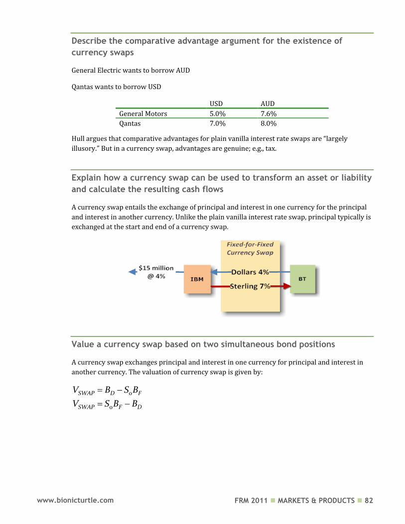
FRM 2011 MARKETS & PRODUCTS 82 www.bionicturtle.com
Describe the comparative advantage argument for the existence of
currency swaps
General Electric wants to borrow AUD
Qantas wants to borrow USD
USD AUD
General Motors 5.0% 7.6%
Qantas 7.0% 8.0%
Hull argues that comparative advantages for plain vanilla interest rate swaps are “largely
illusory.” But in a currency swap, advantages are genuine; e.g., tax.
Explain how a currency swap can be used to transform an asset or liability
and calculate the resulting cash flows
A currency swap entails the exchange of principal and interest in one currency for the principal
and interest in another currency. Unlike the plain vanilla interest rate swap, principal typically is
exchanged at the start and end of a currency swap.
Value a currency swap based on two simultaneous bond positions
A currency swap exchanges principal and interest in one currency for principal and interest in
another currency. The valuation of currency swap is given by:
0
0
SWAP D F
SWAP F D
V B S B
V S B B
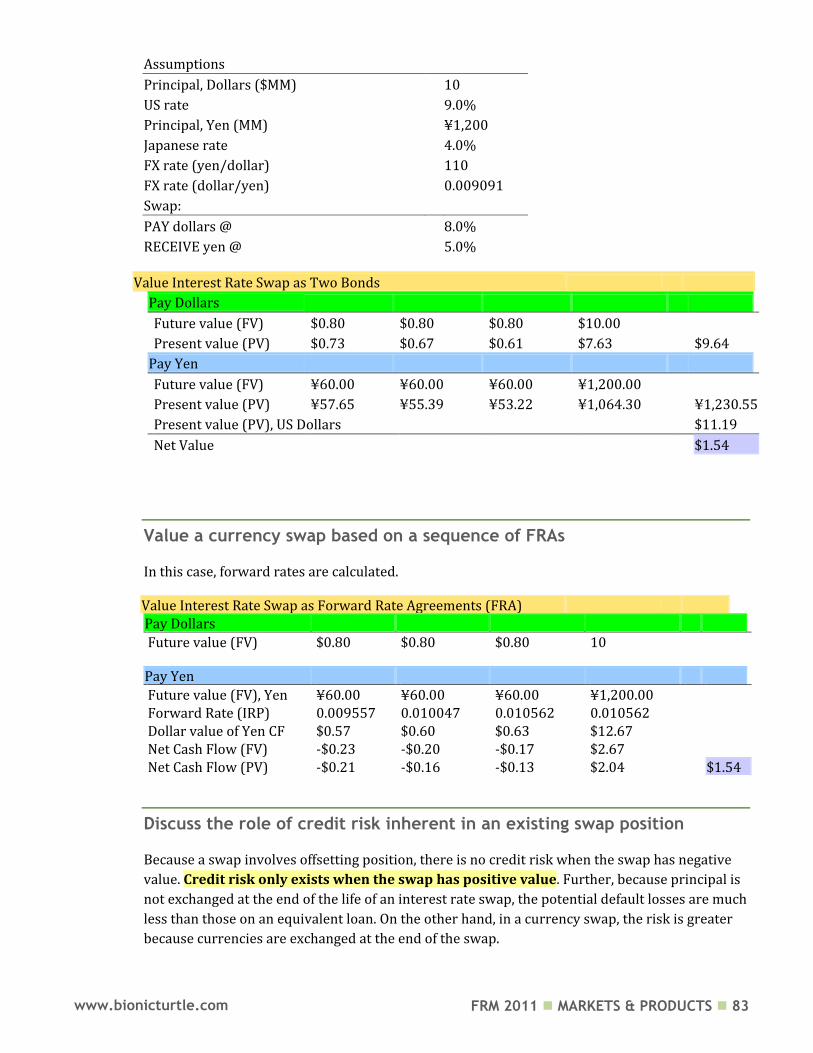
FRM 2011 MARKETS & PRODUCTS 83 www.bionicturtle.com
Value Interest Rate Swap as Two Bonds
Pay Dollars
Future value (FV) $0.80 $0.80 $0.80 $10.00
Present value (PV) $0.73 $0.67 $0.61 $7.63
$9.64
Pay Yen
Future value (FV) ¥60.00 ¥60.00 ¥60.00 ¥1,200.00
Present value (PV) ¥57.65 ¥55.39 ¥53.22 ¥1,064.30
¥1,230.55
Present value (PV), US Dollars
$11.19
Net Value $1.54
Value a currency swap based on a sequence of FRAs
In this case, forward rates are calculated.
Value Interest Rate Swap as Forward Rate Agreements (FRA)
Pay Dollars
Future value (FV) $0.80 $0.80 $0.80 10
Pay Yen
Future value (FV), Yen ¥60.00 ¥60.00 ¥60.00 ¥1,200.00
Forward Rate (IRP) 0.009557 0.010047 0.010562 0.010562
Dollar value of Yen CF $0.57 $0.60 $0.63 $12.67
Net Cash Flow (FV) -$0.23 -$0.20 -$0.17 $2.67
Net Cash Flow (PV) -$0.21 -$0.16 -$0.13 $2.04
$1.54
Discuss the role of credit risk inherent in an existing swap position
Because a swap involves offsetting position, there is no credit risk when the swap has negative
value. Credit risk only exists when the swap has positive value. Further, because principal is
not exchanged at the end of the life of an interest rate swap, the potential default losses are much
less than those on an equivalent loan. On the other hand, in a currency swap, the risk is greater
because currencies are exchanged at the end of the swap.
Assumptions
Principal, Dollars ($MM)
10
US rate
9.0%
Principal, Yen (MM)
¥1,200
Japanese rate
4.0%
FX rate (yen/dollar)
110
FX rate (dollar/yen)
0.009091
Swap:
PAY dollars @
8.0%
RECEIVE yen @
5.0%
FRM 2011 MARKETS & PRODUCTS 84 www.bionicturtle.com
Note the distinction between credit risk and market risk. In the case of a swap,
credit risk includes the risk the counterparty will defaults; market risk includes
the the risk that interest rates and/or currency exchanges rates vary
unfavorably.
List and define other types of swaps, including commodity, volatility and
exotic swaps
The examples in the text refer to a typical “plain vanilla” interest rate swap:
LIBOR is the floating reference rate
Tenor (payment frequency) is six months
Other types of swaps include:
Amortizing Swap: principal reduces in predetermined way
Step-up swap: principal increases
Deferred (forward) swap: parties begin exchange in future
Variations on vanilla fixed-for-floating interest rate swap: tenor is 1 month, 3
months, or 12 months; floating tenor does not match fixed-rate tenor; rates other than
LIBOR (commercial paper)
Principal can vary throught the swap term. Amortizing swap: principal reduces in a
predetermined way. Step-up swap: principle increases in a predetermined way. Forward
(deferred) swap: parties do not begin exchange until some future period.
Constant maturity swap (CMS swap): an agreement to exchange a LIBOR rate for a
swap rate. In a constant maturity Treasury swap (CMT swap), the counterparties agree
to swap a LIBOR rate for a Treasury rate.
Constant maturity Treasury swap: LIBOR for Trate
Compounding swap: interest on one or both sides is compounded forward to the end of
the swap’s life.
LIBOR-in arrears: LIBOR rate used for current (not next) payment.
Accrual: interest on one side accrues if floating rate within a range.
Variations on fixed-for-fixed currency swap. A cross-currency swap is essentially a
fixed-for-floating interest rate swap plus a fixed-for-fixed currency swap. Also, both sides
FRM 2011 MARKETS & PRODUCTS 85 www.bionicturtle.com
can float in a floating-for-floating currency swap. In a diff swap (a.k.a., quanto), a rate
observed in once currency is applied to a principal amount in another currency.
Equity swaps: agreement to exchange total return (gains plus dividends) realized on an
equity index in exchange for LIBOR (both on the same principal).
Options embedded in swaps:
Extendable swap (one counterparty has the option to extend the swap
Puttable (one party has the option to terminate early)
Swaptions (options on swap).
FRM 2011 MARKETS & PRODUCTS 86 www.bionicturtle.com
Hull, Chapter 9:
Properties of Stock
Options
In this chapter…
Identify the six factors that affect an option's price and discuss how these six factors affect the price for both European and American options.
Identify, interpret and compute upper and lower bounds for option prices. Explain put‐call parity and calculate, using the put‐call parity on a non‐dividend‐
paying stock, the value of a European and American option, respectively. Explain the early exercise features of American call and put options on a non‐
dividend‐paying stock and the price effect early exercise may have. Discuss the effects dividends have on the put‐call parity, the bounds of put and
call option prices, and on the early exercise feature of American options.
Notation:
S0 Current stock price
K Strike price (aka, exercise price)
T Time to expiration (aka, term)
ST Stock price at maturity
R Continuously compounded risk-free interest rate
C Value of American call option (option to buy one share)
P Value of American put option (option to sell one share)
c Value of European call option (option to buy one share)
p Value of European put option (option to sell one share)
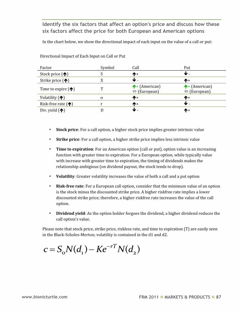
FRM 2011 MARKETS & PRODUCTS 87 www.bionicturtle.com
Identify the six factors that affect an option's price and discuss how these
six factors affect the price for both European and American options
In the chart below, we show the directional impact of each input on the value of a call or put:
Directional Impact of Each Input on Call or Put
Factor Symbol Call Put
Stock price () S + -
Strike price () X - +
Time to expire () T + (American) (European)
+ (American) (European)
Volatility () + +
Risk-free rate () r + -
Div. yield () D - +
Stock price: For a call option, a higher stock price implies greater intrinsic value
Strike price: For a call option, a higher strike price implies less intrinsic value
Time to expiration: For an American option (call or put), option value is an increasing
function with greater time to expiration. For a European option, while typically value
with increase with greater time to expiration, the timing of dividends makes the
relationship ambigious (on dividend payout, the stock tends to drop).
Volatility: Greater volatility increases the value of both a call and a put option
Risk-free rate: For a European call option, consider that the minimum value of an option
is the stock minus the discounted strike price. A higher riskfree rate implies a lower
discounted strike price; therefore, a higher riskfree rate increases the value of the call
option.
Dividend yield: As the option holder forgoes the dividend, a higher dividend reduces the
call option’s value.
Please note that stock price, strike price, riskless rate, and time to expiration (T) are easily seen
in the Black-Scholes-Merton; volatility is contained in the d1 and d2.
0 1 2( ) ( )rTc S N d Ke N d
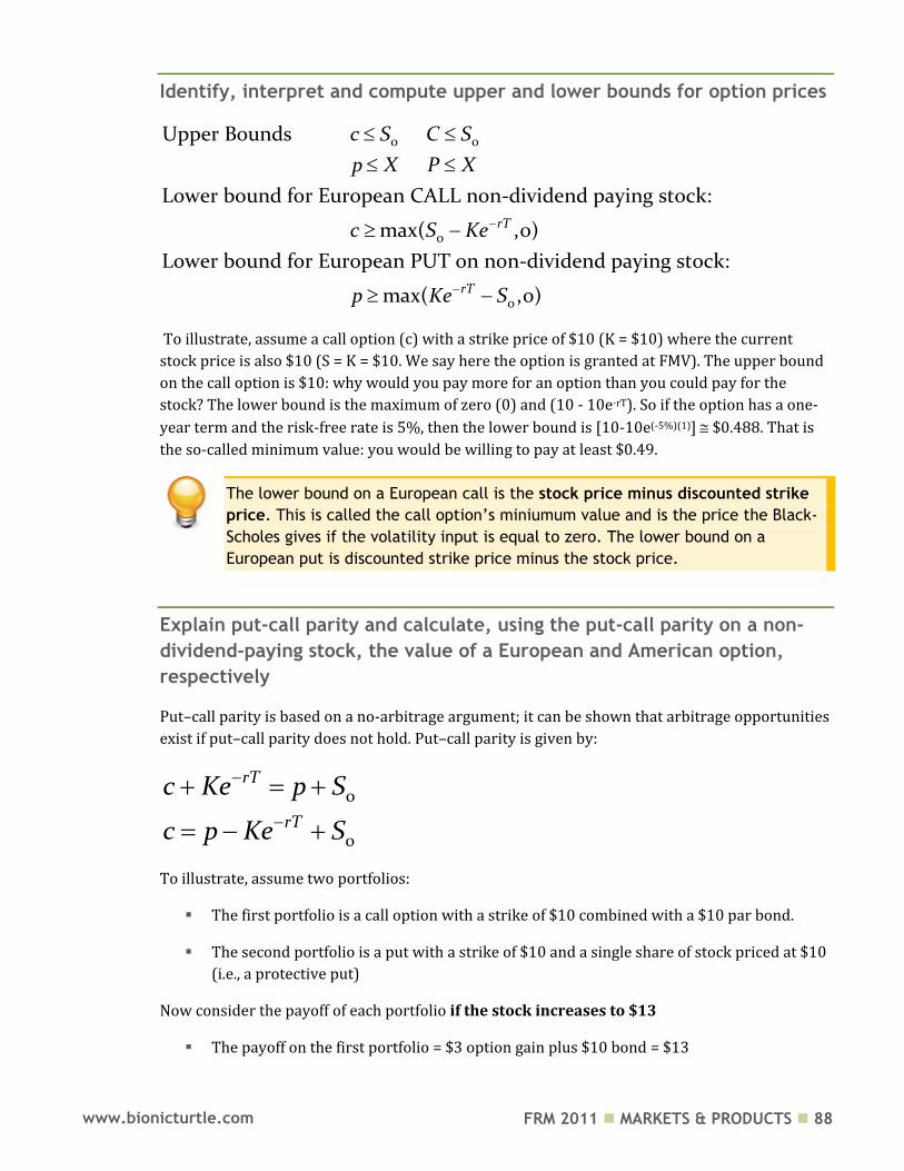
FRM 2011 MARKETS & PRODUCTS 88 www.bionicturtle.com
Identify, interpret and compute upper and lower bounds for option prices
0 0
0
0
Upper Bounds
Lower bound for European CALL non-dividend paying stock:
max( ,0)
Lower bound for European PUT on non-dividend paying stock:
max( ,0)
rT
rT
c S C S
p X P X
c S Ke
p Ke S
To illustrate, assume a call option (c) with a strike price of $10 (K = $10) where the current
stock price is also $10 (S = K = $10. We say here the option is granted at FMV). The upper bound
on the call option is $10: why would you pay more for an option than you could pay for the
stock? The lower bound is the maximum of zero (0) and (10 - 10e-rT). So if the option has a one-
year term and the risk-free rate is 5%, then the lower bound is [10-10e(-5%)(1)] $0.488. That is
the so-called minimum value: you would be willing to pay at least $0.49.
The lower bound on a European call is the stock price minus discounted strike
price. This is called the call option’s miniumum value and is the price the Black-
Scholes gives if the volatility input is equal to zero. The lower bound on a
European put is discounted strike price minus the stock price.
Explain put‐call parity and calculate, using the put‐call parity on a non‐
dividend‐paying stock, the value of a European and American option,
respectively
Put–call parity is based on a no-arbitrage argument; it can be shown that arbitrage opportunities
exist if put–call parity does not hold. Put–call parity is given by:
0
0
rT
rT
c Ke p S
c p Ke S
To illustrate, assume two portfolios:
The first portfolio is a call option with a strike of $10 combined with a $10 par bond.
The second portfolio is a put with a strike of $10 and a single share of stock priced at $10
(i.e., a protective put)
Now consider the payoff of each portfolio if the stock increases to $13
The payoff on the first portfolio = $3 option gain plus $10 bond = $13
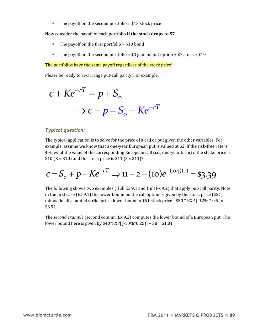
FRM 2011 MARKETS & PRODUCTS 89 www.bionicturtle.com
The payoff on the second portfolio = $13 stock price
Now consider the payoff of each portfolio if the stock drops to $7
The payoff on the first portfolio = $10 bond
The payoff on the second portfolio = $3 gain on put option + $7 stock = $10
The portfolios have the same payoff regardless of the stock price!
Please be ready to re-arrange put-call parity. For example:
Typical question:
The typical application is to solve for the price of a call or put given the other variables. For
example, assume we know that a one-year European put is valued at $2. If the risk-free rate is
4%, what the value of the corresponding European call (i.e., one-year term) if the strike price is
$10 (K = $10) and the stock price is $11 (S = $11)?
(.04)(1)0 11 2 (10) $3.39rTc S p Ke e
The following shows two examples (Hull Ex 9.1 and Hull Ex 9.2) that apply put-call parity. Note
in the first case (Ex 9.1) the lower bound on the call option is given by the stock price ($51)
minus the discounted strike price: lower bound = $51 stock price - $50 * EXP [-12% * 0.5] =
$3.91.
The second example (second column, Ex 9.2) computes the lower bound of a European put. The
lower bound here is given by $40*EXP[(-10%*0.25)] – 38 = $1.01
Forward
(F0)
0
0rT
rT
c p S
c S
Ke
Ke p
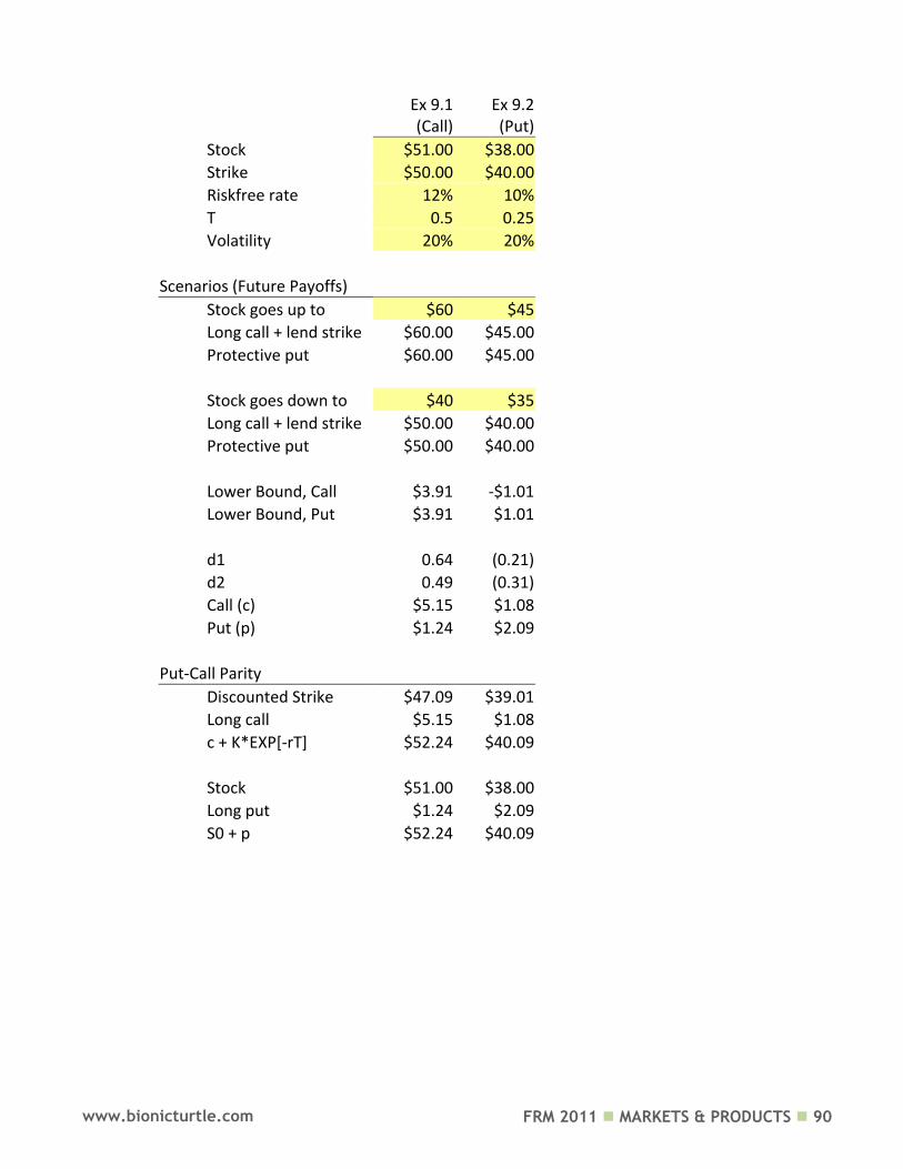
FRM 2011 MARKETS & PRODUCTS 90 www.bionicturtle.com
Ex 9.1 (Call)
Ex 9.2 (Put)
Stock $51.00 $38.00
Strike $50.00 $40.00
Riskfree rate 12% 10%
T 0.5 0.25
Volatility 20% 20%
Scenarios (Future Payoffs)
Stock goes up to $60 $45
Long call + lend strike $60.00 $45.00
Protective put $60.00 $45.00
Stock goes down to $40 $35
Long call + lend strike $50.00 $40.00
Protective put $50.00 $40.00
Lower Bound, Call $3.91 -$1.01
Lower Bound, Put $3.91 $1.01
d1 0.64 (0.21)
d2 0.49 (0.31)
Call (c) $5.15 $1.08
Put (p) $1.24 $2.09
Put-Call Parity
Discounted Strike $47.09 $39.01
Long call $5.15 $1.08
c + K*EXP[-rT] $52.24 $40.09
Stock $51.00 $38.00
Long put $1.24 $2.09
S0 + p $52.24 $40.09
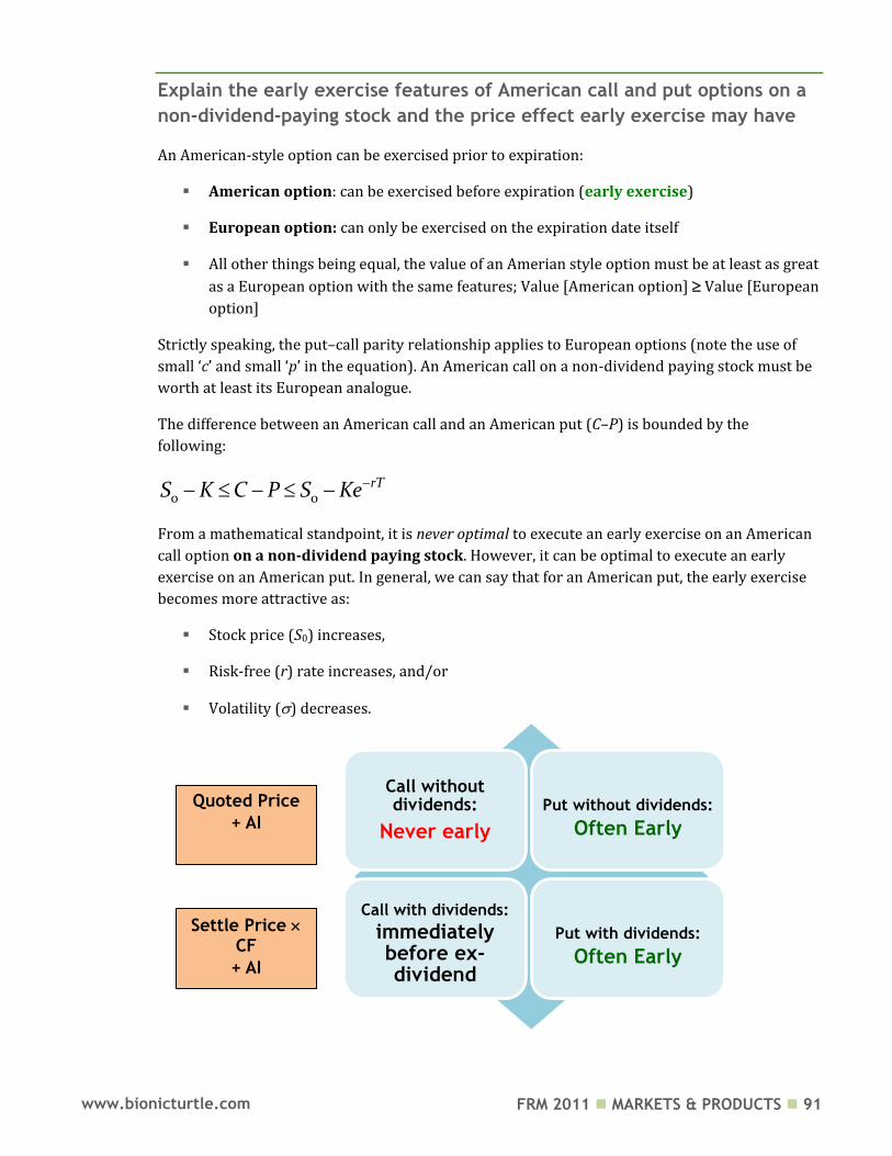
FRM 2011 MARKETS & PRODUCTS 91 www.bionicturtle.com
Explain the early exercise features of American call and put options on a
non‐dividend‐paying stock and the price effect early exercise may have
An American-style option can be exercised prior to expiration:
American option: can be exercised before expiration (early exercise)
European option: can only be exercised on the expiration date itself
All other things being equal, the value of an Amerian style option must be at least as great
as a European option with the same features; Value [American option] Value [European
option]
Strictly speaking, the put–call parity relationship applies to European options (note the use of
small ‘c’ and small ‘p’ in the equation). An American call on a non-dividend paying stock must be
worth at least its European analogue.
The difference between an American call and an American put (C–P) is bounded by the
following:
0 0rTS K C P S Ke
From a mathematical standpoint, it is never optimal to execute an early exercise on an American
call option on a non-dividend paying stock. However, it can be optimal to execute an early
exercise on an American put. In general, we can say that for an American put, the early exercise
becomes more attractive as:
Stock price (S0) increases,
Risk-free (r) rate increases, and/or
Volatility () decreases.
Call without dividends:
Never early
Put without dividends: Often Early
Call with dividends: immediately before ex-dividend
Put with dividends: Often Early
Quoted Price
+ AI
Settle Price CF
+ AI
FRM 2011 MARKETS & PRODUCTS 92 www.bionicturtle.com
Discuss the effects dividends have on the put‐call parity, the bounds of
put and call option prices, and on the early exercise feature of American
options
The ex-dividend date is specified when a dividend is declared. Investors who own shares of the
stock as of the ex-dividend date receive the dividend.
An American option should never be exercised early in the absence of dividends. In the case of
a dividend-paying stock, it would only be optimal to exercise immediately before the stock
goes ex-dividend. Specifically, early exercise would remain sub-optimal if the following
inequality applied:
( )1(1 )r t ti iiD K e
Further, this inequality applies unless the dividend yield is “either close to or above the risk-free
rate of interest”, which typically is not the case. Therefore, early exercise remains sub-optimal in
most cases.
Put–call parity applies to European options (note the use of small ‘c’ and small ‘p’ in the
equation).
An American call on a non-dividend paying stock must be worth at least its European
analogue
The difference between an American call and an American put (C–P) is bounded by the
following:
0 0rTS K C P S Ke
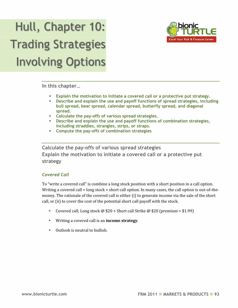
FRM 2011 MARKETS & PRODUCTS 93 www.bionicturtle.com
Hull, Chapter 10:
Trading Strategies
Involving Options
In this chapter…
Explain the motivation to initiate a covered call or a protective put strategy. Describe and explain the use and payoff functions of spread strategies, including
bull spread, bear spread, calendar spread, butterfly spread, and diagonal spread.
Calculate the pay‐offs of various spread strategies. Describe and explain the use and payoff functions of combination strategies,
including straddles, strangles, strips, or straps. Compute the pay‐offs of combination strategies
Calculate the pay‐offs of various spread strategies
Explain the motivation to initiate a covered call or a protective put
strategy
Covered Call
To “write a covered call” is combine a long stock position with a short position in a call option.
Writing a covered call = long stock + short call option. In many cases, the call option is out-of-the-
money. The rationale of the covered call is either (i) to generate income via the sale of the short
call, or (ii) to cover the cost of the potential short call payoff with the stock.
Covered call; Long stock @ $20 + Short call Strike @ $20 (premium = $1.99)
Writing a covered call is an income strategy.
Outlook is neutral to bullish.
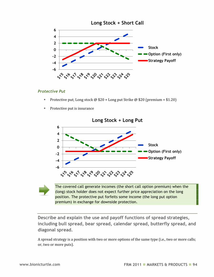
FRM 2011 MARKETS & PRODUCTS 94 www.bionicturtle.com
Protective Put
Protective put; Long stock @ $20 + Long put Strike @ $20 (premium = $1.20)
Protective put is insurance
The covered call generate incomes (the short call option premium) when the
(long) stock holder does not expect further price appreciation on the long
position. The protective put forfeits some income (the long put option
premium) in exchange for downside protection.
Describe and explain the use and payoff functions of spread strategies,
including bull spread, bear spread, calendar spread, butterfly spread, and
diagonal spread.
A spread strategy is a position with two or more options of the same type (i.e., two or more calls;
or, two or more puts).
-6
-4
-2
0
2
4
6
Long Stock + Short Call
Stock
Option (First only)
Strategy Payoff
-6
-4
-2
0
2
4
6
Long Stock + Long Put
Stock
Option (First only)
Strategy Payoff
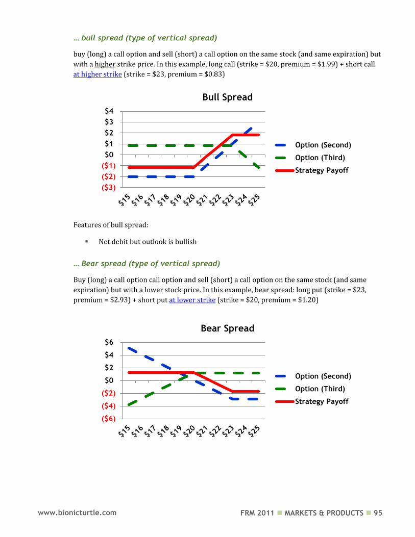
FRM 2011 MARKETS & PRODUCTS 95 www.bionicturtle.com
… bull spread (type of vertical spread)
buy (long) a call option and sell (short) a call option on the same stock (and same expiration) but
with a higher strike price. In this example, long call (strike = $20, premium = $1.99) + short call
at higher strike (strike = $23, premium = $0.83)
Features of bull spread:
Net debit but outlook is bullish
… Bear spread (type of vertical spread)
Buy (long) a call option call option and sell (short) a call option on the same stock (and same
expiration) but with a lower stock price. In this example, bear spread: long put (strike = $23,
premium = $2.93) + short put at lower strike (strike = $20, premium = $1.20)
($3)
($2)
($1)
$0
$1
$2
$3
$4
Bull Spread
Option (Second)
Option (Third)
Strategy Payoff
($6)
($4)
($2)
$0
$2
$4
$6
Bear Spread
Option (Second)
Option (Third)
Strategy Payoff
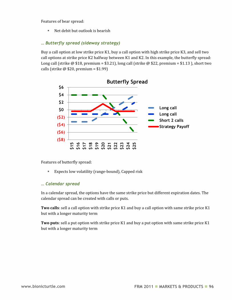
FRM 2011 MARKETS & PRODUCTS 96 www.bionicturtle.com
Features of bear spread:
Net debit but outlook is bearish
… Butterfly spread (sideway strategy)
Buy a call option at low strike price K1, buy a call option with high strike price K3, and sell two
call options at strike price K2 halfway between K1 and K2. In this example, the butterfly spread:
Long call (strike @ $18, premium = $3.21), long call (strike @ $22, premium = $1.13 ), short two
calls (strike @ $20, premium = $1.99)
Features of butterfly spread:
Expects low volatility (range-bound), Capped risk
… Calendar spread
In a calendar spread, the options have the same strike price but different expiration dates. The
calendar spread can be created with calls or puts.
Two calls: sell a call option with strike price K1 and buy a call option with same strike price K1
but with a longer maturity term
Two puts: sell a put option with strike price K1 and buy a put option with same strike price K1
but with a longer maturity term
($8)
($6)
($4)
($2)
$0
$2
$4
$6
$15
$16
$17
$18
$19
$20
$21
$22
$23
$24
$25
Butterfly Spread
Long call
Long call
Short 2 calls
Strategy Payoff
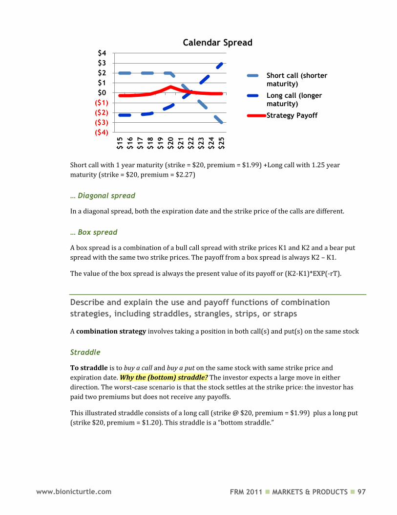
FRM 2011 MARKETS & PRODUCTS 97 www.bionicturtle.com
Short call with 1 year maturity (strike = $20, premium = $1.99) +Long call with 1.25 year
maturity (strike = $20, premium = $2.27)
… Diagonal spread
In a diagonal spread, both the expiration date and the strike price of the calls are different.
… Box spread
A box spread is a combination of a bull call spread with strike prices K1 and K2 and a bear put
spread with the same two strike prices. The payoff from a box spread is always K2 – K1.
The value of the box spread is always the present value of its payoff or (K2-K1)*EXP(-rT).
Describe and explain the use and payoff functions of combination
strategies, including straddles, strangles, strips, or straps
A combination strategy involves taking a position in both call(s) and put(s) on the same stock
Straddle
To straddle is to buy a call and buy a put on the same stock with same strike price and
expiration date. Why the (bottom) straddle? The investor expects a large move in either
direction. The worst-case scenario is that the stock settles at the strike price: the investor has
paid two premiums but does not receive any payoffs.
This illustrated straddle consists of a long call (strike @ $20, premium = $1.99) plus a long put
(strike $20, premium = $1.20). This straddle is a “bottom straddle.”
($4)
($3)
($2)
($1)
$0
$1
$2
$3
$4
$15
$16
$17
$18
$19
$20
$21
$22
$23
$24
$25
Calendar Spread
Short call (shortermaturity)
Long call (longermaturity)
Strategy Payoff
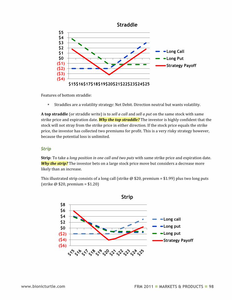
FRM 2011 MARKETS & PRODUCTS 98 www.bionicturtle.com
Features of bottom straddle:
Straddles are a volatility strategy: Net Debit. Direction neutral but wants volatility.
A top straddle (or straddle write) is to sell a call and sell a put on the same stock with same
strike price and expiration date. Why the top straddle? The investor is highly confident that the
stock will not stray from the strike price in either direction. If the stock price equals the strike
price, the investor has collected two premiums for profit. This is a very risky strategy however,
because the potential loss is unlimited.
Strip
Strip: To take a long position in one call and two puts with same strike price and expiration date.
Why the strip? The investor bets on a large stock price move but considers a decrease more
likely than an increase.
This illustrated strip consists of a long call (strike @ $20, premium = $1.99) plus two long puts
(strike @ $20, premium = $1.20)
($4)
($3)
($2)
($1)
$0
$1
$2
$3
$4
$5
$15$16$17$18$19$20$21$22$23$24$25
Straddle
Long Call
Long Put
Strategy Payoff
($6)
($4)
($2)
$0
$2
$4
$6
$8
Strip
Long call
Long put
Long put
Strategy Payoff
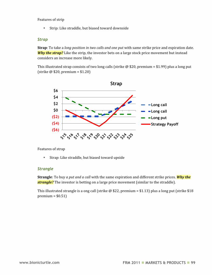
FRM 2011 MARKETS & PRODUCTS 99 www.bionicturtle.com
Features of strip
Strip: Like straddle, but biased toward downside
Strap
Strap: To take a long position in two calls and one put with same strike price and expiration date.
Why the strap? Like the strip, the investor bets on a large stock price movement but instead
considers an increase more likely.
This illustrated strap consists of two long calls (strike @ $20, premium = $1.99) plus a long put
(strike @ $20, premium = $1.20)
Features of strap
Strap: Like straddle, but biased toward upside
Strangle
Strangle: To buy a put and a call with the same expiration and different strike prices. Why the
strangle? The investor is betting on a large price movement (similar to the straddle).
This illustrated strangle is a ong call (strike @ $22, premium = $1.13) plus a long put (strike $18
premium = $0.51)
($6)
($4)
($2)
$0
$2
$4
$6
Strap
Long call
Long call
Long put
Strategy Payoff
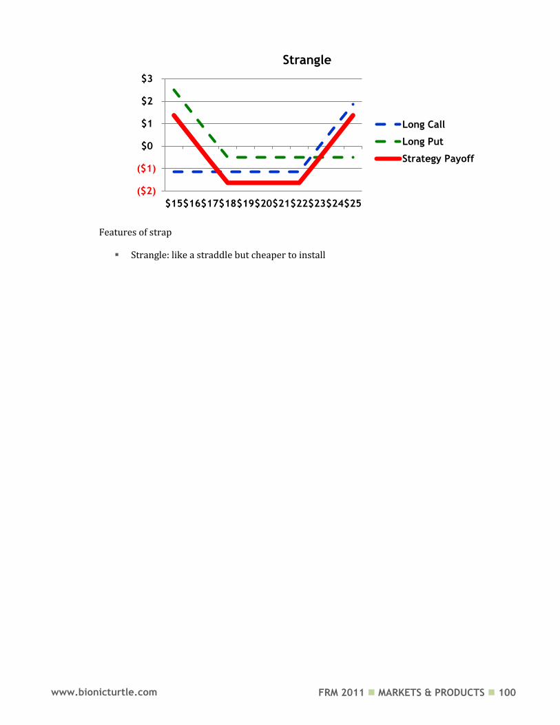
FRM 2011 MARKETS & PRODUCTS 100 www.bionicturtle.com
Features of strap
Strangle: like a straddle but cheaper to install
($2)
($1)
$0
$1
$2
$3
$15$16$17$18$19$20$21$22$23$24$25
Strangle
Long Call
Long Put
Strategy Payoff
FRM 2011 MARKETS & PRODUCTS 101 www.bionicturtle.com
McDonald, Chapter
6: Commodity
Forwards and
Futures
In this chapter…
Define forward strip and forward curve. Describe how to create a synthetic commodity position and use it to explain the
relationship between the forward price and the expected future spot price. Explain the effect non‐storability has on electricity prices. Derive the basic equilibrium formula for pricing commodity forwards and
futures. Explain the implication basic equilibrium has for different types of commodities. Describe an arbitrage transaction in commodity forwards and futures, and
compute the potential arbitrage profit. Define the lease rate and how it determines the no‐arbitrage values for
commodity forwards and futures, and explain the relationship between lease rates and contango and lease rates and backwardation, respectively.
Define carry markets. Explain the impact storage costs and convenience yields have on commodity
forward prices and no‐arbitrage bounds. Compute the forward price of a commodity with storage costs. Compare the lease rate with the convenience yield. Discuss factors that impact gold, corn, natural gas, and crude oil futures prices. Define and compute a commodity spread. Explain how basis risk can occur when hedging commodity price exposure. Evaluate the differences between a strip hedge and a stack hedge and analyze
how these differences impact risk management.
Define forward strip and forward curve
On any given day, for any given commodity, there are different futures contracts available that
expire in different months; i.e., these contracts have different maturities.
The set of prices for different expiration dates for a given commodity is called the forward
curve for the forward strip for the date
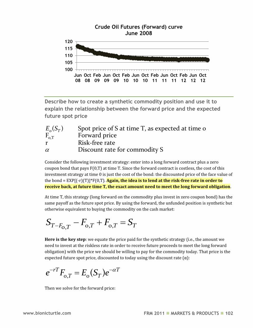
FRM 2011 MARKETS & PRODUCTS 102 www.bionicturtle.com
Describe how to create a synthetic commodity position and use it to
explain the relationship between the forward price and the expected
future spot price
0
0,T
( ) Spot price of S at time T, as expected at time 0F Forward pricer Risk-free rate
Discount rate for commodity S
TE S
Consider the following investment strategy: enter into a long forward contract plus a zero
coupon bond that pays F(0,T) at time T. Since the forward contract is costless, the cost of this
investment strategy at time 0 is just the cost of the bond: the discounted price of the face value of
the bond = EXP[(-r)(T)]*F(0,T). Again, the idea is to lend at the risk-free rate in order to
receive back, at future time T, the exact amount need to meet the long forward obligation.
At time T, this strategy (long forward on the commodity plus invest in zero coupon bond) has the
same payoff as the future spot price. By using the forward, the unfunded position is synthetic but
otherwise equivalent to buying the commodity on the cash market:
0, 0,0,T F T T TTS F F S
Here is the key step: we equate the price paid for the synthetic strategy (i.e., the amount we
need to invest at the riskless rate in order to receive future proceeds to meet the long forward
obligation) with the price we should be willing to pay for the commodity today. That price is the
expected future spot price, discounted to today using the discount rate (α):
0, 0( )rT TT Te F E S e
Then we solve for the forward price:
100
105
110
115
120
Jun08
Oct08
Feb09
Jun09
Oct09
Feb10
Jun10
Oct10
Feb11
Jun11
Oct11
Feb12
Jun12
Oct12
Crude Oil Futures (Forward) curve June 2008
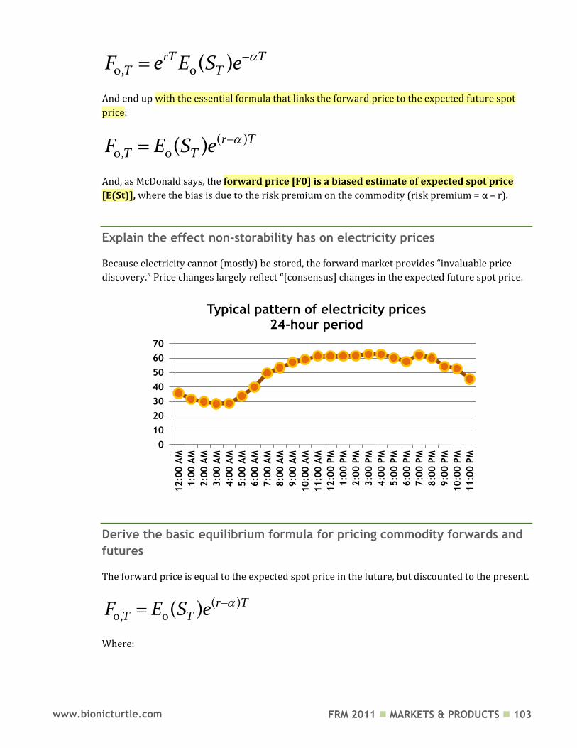
FRM 2011 MARKETS & PRODUCTS 103 www.bionicturtle.com
0, 0( )rT TT TF e E S e
And end up with the essential formula that links the forward price to the expected future spot
price:
( )0, 0( ) r TT TF E S e
And, as McDonald says, the forward price [F0] is a biased estimate of expected spot price
[E(St)], where the bias is due to the risk premium on the commodity (risk premium = α – r).
Explain the effect non‐storability has on electricity prices
Because electricity cannot (mostly) be stored, the forward market provides “invaluable price
discovery.” Price changes largely reflect “[consensus] changes in the expected future spot price.
Derive the basic equilibrium formula for pricing commodity forwards and
futures
The forward price is equal to the expected spot price in the future, but discounted to the present.
( )0, 0( ) r TT TF E S e
Where:
0
10
20
30
40
50
60
70
12:0
0 A
M
1:0
0 A
M
2:0
0 A
M
3:0
0 A
M
4:0
0 A
M
5:0
0 A
M
6:0
0 A
M
7:0
0 A
M
8:0
0 A
M
9:0
0 A
M
10:0
0 A
M
11:0
0 A
M
12:0
0 P
M
1:0
0 P
M
2:0
0 P
M
3:0
0 P
M
4:0
0 P
M
5:0
0 P
M
6:0
0 P
M
7:0
0 P
M
8:0
0 P
M
9:0
0 P
M
10:0
0 P
M
11:0
0 P
M
Typical pattern of electricity prices 24-hour period
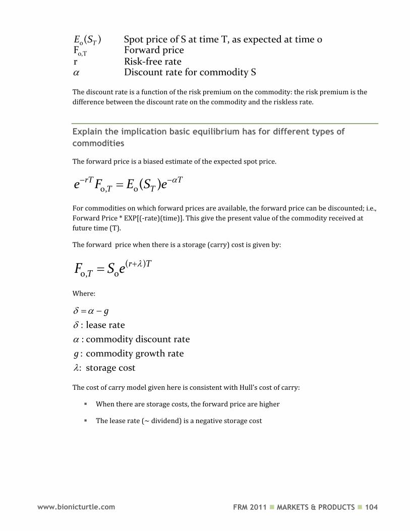
FRM 2011 MARKETS & PRODUCTS 104 www.bionicturtle.com
0
0,T
( ) Spot price of S at time T, as expected at time 0F Forward pricer Risk-free rate
Discount rate for commodity S
TE S
The discount rate is a function of the risk premium on the commodity: the risk premium is the
difference between the discount rate on the commodity and the riskless rate.
Explain the implication basic equilibrium has for different types of
commodities
The forward price is a biased estimate of the expected spot price.
0, 0( )rT TT Te F E S e
For commodities on which forward prices are available, the forward price can be discounted; i.e.,
Forward Price * EXP[(-rate)(time)]. This give the present value of the commodity received at
future time (T).
The forward price when there is a storage (carry) cost is given by:
( )0, 0
r TTF S e
Where:
: lease rate
: commodity discount rate
: commodity growth rate
: storage cost
g
g
The cost of carry model given here is consistent with Hull’s cost of carry:
When there are storage costs, the forward price are higher
The lease rate (~ dividend) is a negative storage cost
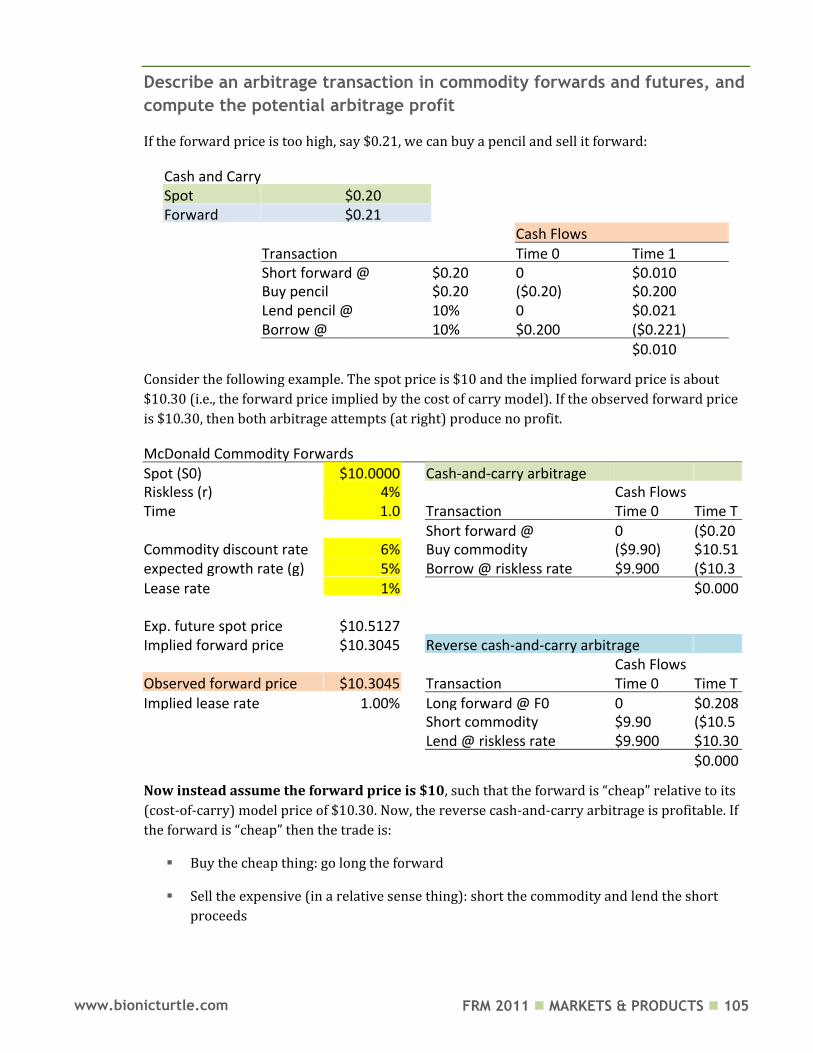
FRM 2011 MARKETS & PRODUCTS 105 www.bionicturtle.com
Describe an arbitrage transaction in commodity forwards and futures, and
compute the potential arbitrage profit
If the forward price is too high, say $0.21, we can buy a pencil and sell it forward:
Cash and Carry
Spot $0.20 Forward $0.21
Cash Flows
Transaction Time 0 Time 1
Short forward @ $0.20 0 $0.010
Buy pencil $0.20 ($0.20) $0.200
Lend pencil @ 10% 0 $0.021
Borrow @ 10% $0.200 ($0.221)
$0.010
Consider the following example. The spot price is $10 and the implied forward price is about
$10.30 (i.e., the forward price implied by the cost of carry model). If the observed forward price
is $10.30, then both arbitrage attempts (at right) produce no profit.
McDonald Commodity Forwards Spot (S0)
$10.0000
Cash-and-carry arbitrage
Riskless (r)
4%
Cash Flows Time
1.0
Transaction Time 0 Time T
Short forward @ F0
0 ($0.20
8) Commodity discount rate (alpha)
6%
Buy commodity
($9.90) $10.513 expected growth rate (g) 5%
Borrow @ riskless rate $9.900 ($10.3
05) Lease rate
1%
$0.0000
Exp. future spot price $10.5127
Implied forward price $10.3045
Reverse cash-and-carry arbitrage
Cash Flows Observed forward price $10.3045
Transaction Time 0 Time T
Implied lease rate 1.00%
Long forward @ F0
0 $0.208
Short commodity
$9.90 ($10.5
13)
Lend @ riskless rate $9.900 $10.305
$0.0000
Now instead assume the forward price is $10, such that the forward is “cheap” relative to its
(cost-of-carry) model price of $10.30. Now, the reverse cash-and-carry arbitrage is profitable. If
the forward is “cheap” then the trade is:
Buy the cheap thing: go long the forward
Sell the expensive (in a relative sense thing): short the commodity and lend the short
proceeds
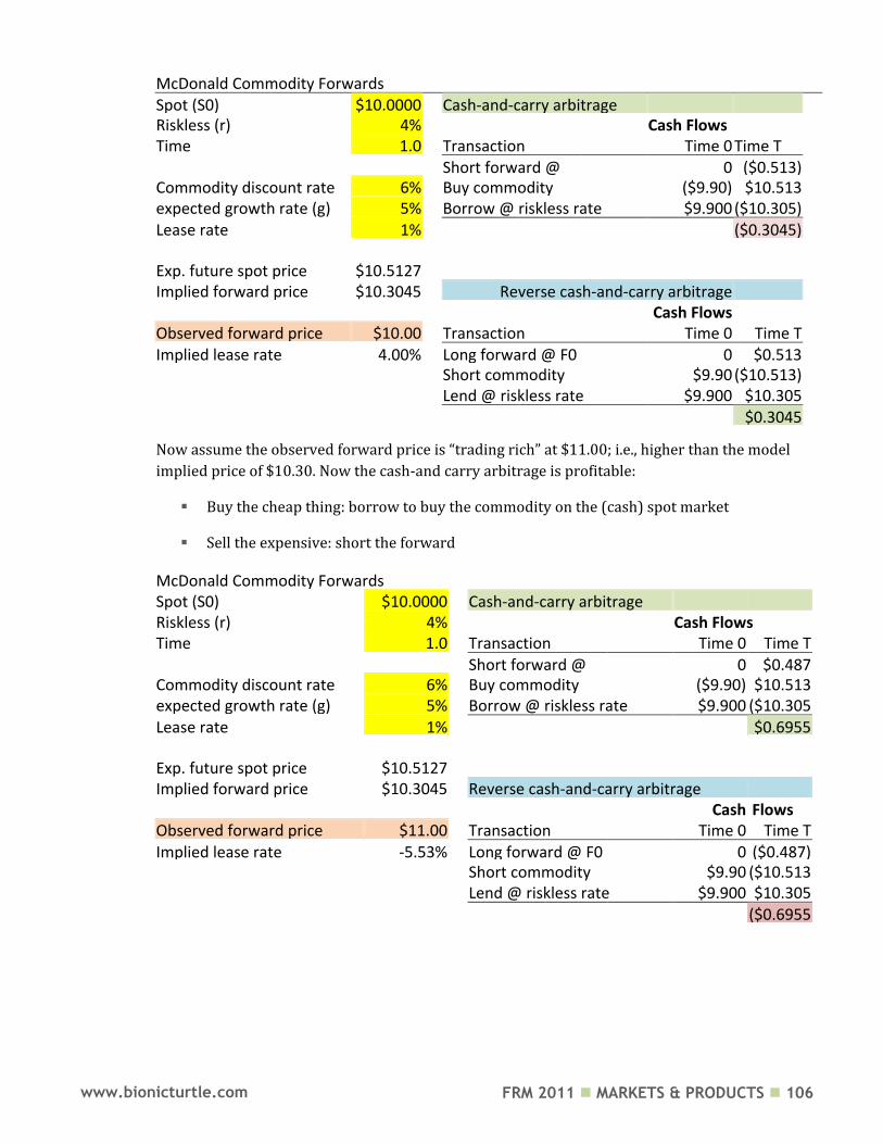
FRM 2011 MARKETS & PRODUCTS 106 www.bionicturtle.com
McDonald Commodity Forwards Spot (S0)
$10.0000
Cash-and-carry arbitrage
Riskless (r)
4%
Cash Flows Time
1.0
Transaction Time 0 Time T
Short forward @ F0
0 ($0.513)
Commodity discount rate (alpha)
6%
Buy commodity
($9.90) $10.513 expected growth rate (g) 5%
Borrow @ riskless rate $9.900 ($10.305)
Lease rate
1%
($0.3045)
Exp. future spot price $10.5127
Implied forward price $10.3045
Reverse cash-and-carry arbitrage
Cash Flows Observed forward price $10.00
Transaction Time 0 Time T
Implied lease rate 4.00%
Long forward @ F0
0 $0.513
Short commodity
$9.90 ($10.513)
Lend @ riskless rate $9.900 $10.305
$0.3045
Now assume the observed forward price is “trading rich” at $11.00; i.e., higher than the model
implied price of $10.30. Now the cash-and carry arbitrage is profitable:
Buy the cheap thing: borrow to buy the commodity on the (cash) spot market
Sell the expensive: short the forward
McDonald Commodity Forwards Spot (S0)
$10.0000
Cash-and-carry arbitrage
Riskless (r)
4%
Cash Flows Time
1.0
Transaction Time 0 Time T
Short forward @ F0
0 $0.487
Commodity discount rate (alpha)
6%
Buy commodity
($9.90) $10.513 expected growth rate (g) 5%
Borrow @ riskless rate $9.900 ($10.305
) Lease rate
1%
$0.6955
Exp. future spot price $10.5127
Implied forward price $10.3045
Reverse cash-and-carry arbitrage
Cash Flows
Flows Observed forward price $11.00
Transaction Time 0 Time T
Implied lease rate -5.53%
Long forward @ F0
0 ($0.487)
Short commodity
$9.90 ($10.513
)
Lend @ riskless rate $9.900 $10.305
($0.6955
)
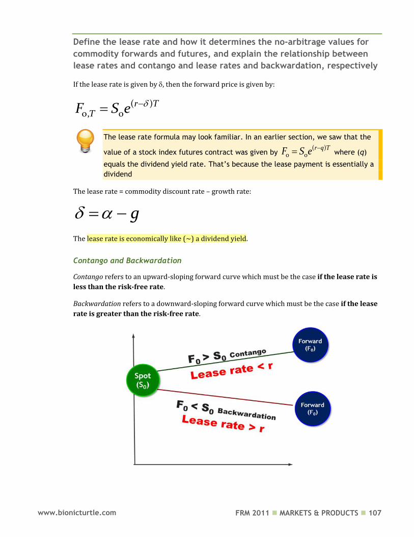
FRM 2011 MARKETS & PRODUCTS 107 www.bionicturtle.com
Define the lease rate and how it determines the no‐arbitrage values for
commodity forwards and futures, and explain the relationship between
lease rates and contango and lease rates and backwardation, respectively
If the lease rate is given by , then the forward price is given by:
( )0, 0
r TTF S e
The lease rate formula may look familiar. In an earlier section, we saw that the
value of a stock index futures contract was given by ( )
0 0r q TF S e where (q)
equals the dividend yield rate. That’s because the lease payment is essentially a
dividend
The lease rate = commodity discount rate – growth rate:
g
The lease rate is economically like (~) a dividend yield.
Contango and Backwardation
Contango refers to an upward-sloping forward curve which must be the case if the lease rate is
less than the risk-free rate.
Backwardation refers to a downward-sloping forward curve which must be the case if the lease
rate is greater than the risk-free rate.
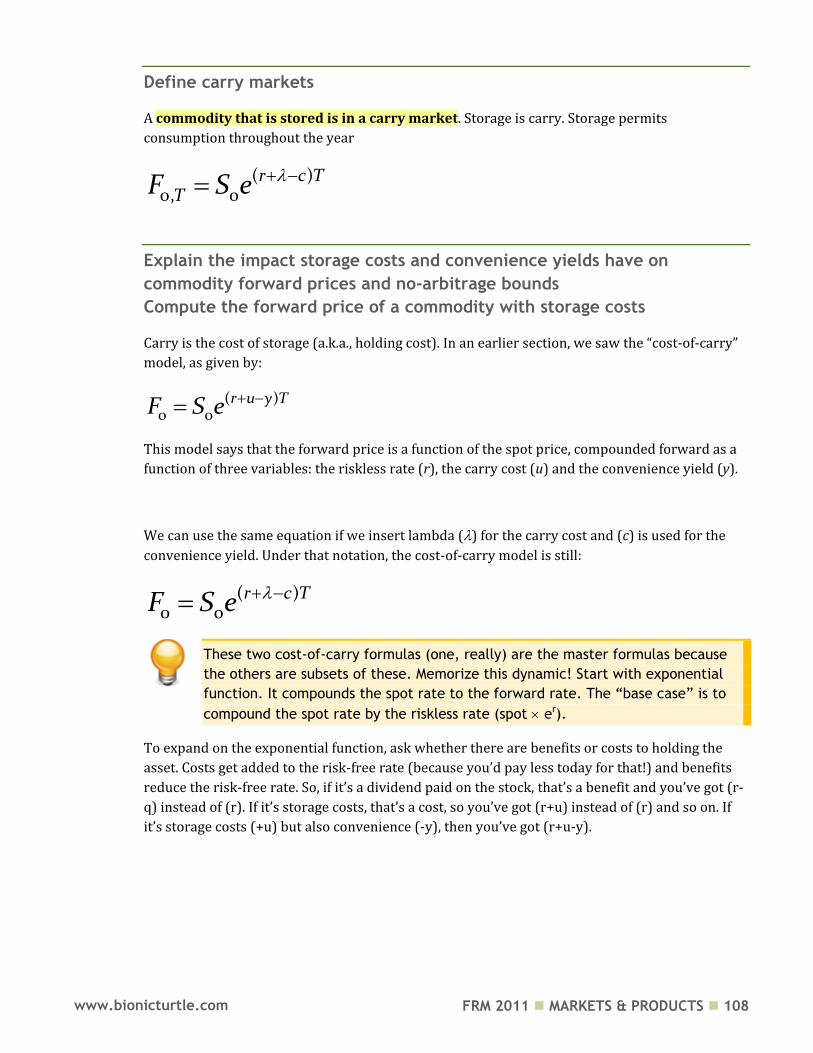
FRM 2011 MARKETS & PRODUCTS 108 www.bionicturtle.com
Define carry markets
A commodity that is stored is in a carry market. Storage is carry. Storage permits
consumption throughout the year
( )0, 0
r c TTF S e
Explain the impact storage costs and convenience yields have on
commodity forward prices and no‐arbitrage bounds
Compute the forward price of a commodity with storage costs
Carry is the cost of storage (a.k.a., holding cost). In an earlier section, we saw the “cost-of-carry”
model, as given by:
( )0 0
r u y TF S e
This model says that the forward price is a function of the spot price, compounded forward as a
function of three variables: the riskless rate (r), the carry cost (u) and the convenience yield (y).
We can use the same equation if we insert lambda () for the carry cost and (c) is used for the
convenience yield. Under that notation, the cost-of-carry model is still:
( )0 0
r c TF S e
These two cost-of-carry formulas (one, really) are the master formulas because
the others are subsets of these. Memorize this dynamic! Start with exponential
function. It compounds the spot rate to the forward rate. The “base case” is to
compound the spot rate by the riskless rate (spot er).
To expand on the exponential function, ask whether there are benefits or costs to holding the
asset. Costs get added to the risk-free rate (because you’d pay less today for that!) and benefits
reduce the risk-free rate. So, if it’s a dividend paid on the stock, that’s a benefit and you’ve got (r-
q) instead of (r). If it’s storage costs, that’s a cost, so you’ve got (r+u) instead of (r) and so on. If
it’s storage costs (+u) but also convenience (-y), then you’ve got (r+u-y).
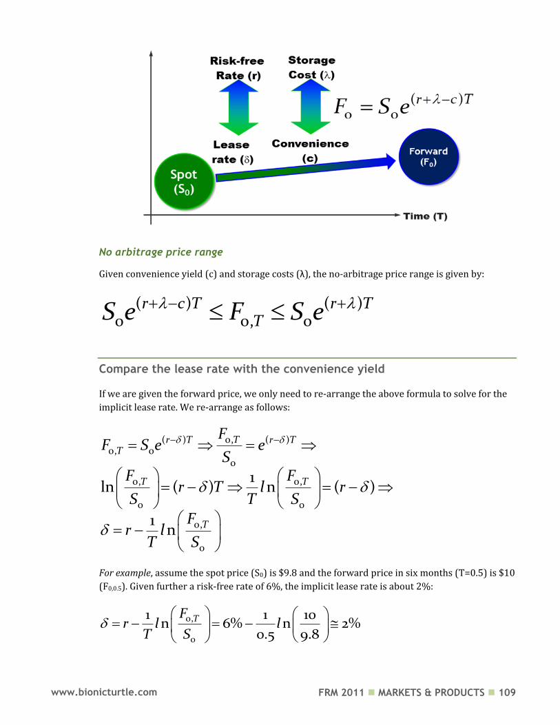
FRM 2011 MARKETS & PRODUCTS 109 www.bionicturtle.com
No arbitrage price range
Given convenience yield (c) and storage costs (λ), the no-arbitrage price range is given by:
( ) ( )0 0, 0
r c T r TTS e F S e
Compare the lease rate with the convenience yield
If we are given the forward price, we only need to re-arrange the above formula to solve for the
implicit lease rate. We re-arrange as follows:
0,( ) ( )0, 0
0
0, 0,
0 0
0,
0
1ln ( ) n ( )
1n
Tr T r TT
T T
T
FF S e e
SF F
r T l rS T S
Fr l
T S
For example, assume the spot price (S0) is $9.8 and the forward price in six months (T=0.5) is $10
(F0,0.5). Given further a risk-free rate of 6%, the implicit lease rate is about 2%:
0,
0
1 1 10n 6% n 2%
0.5 9.8TF
r l lT S
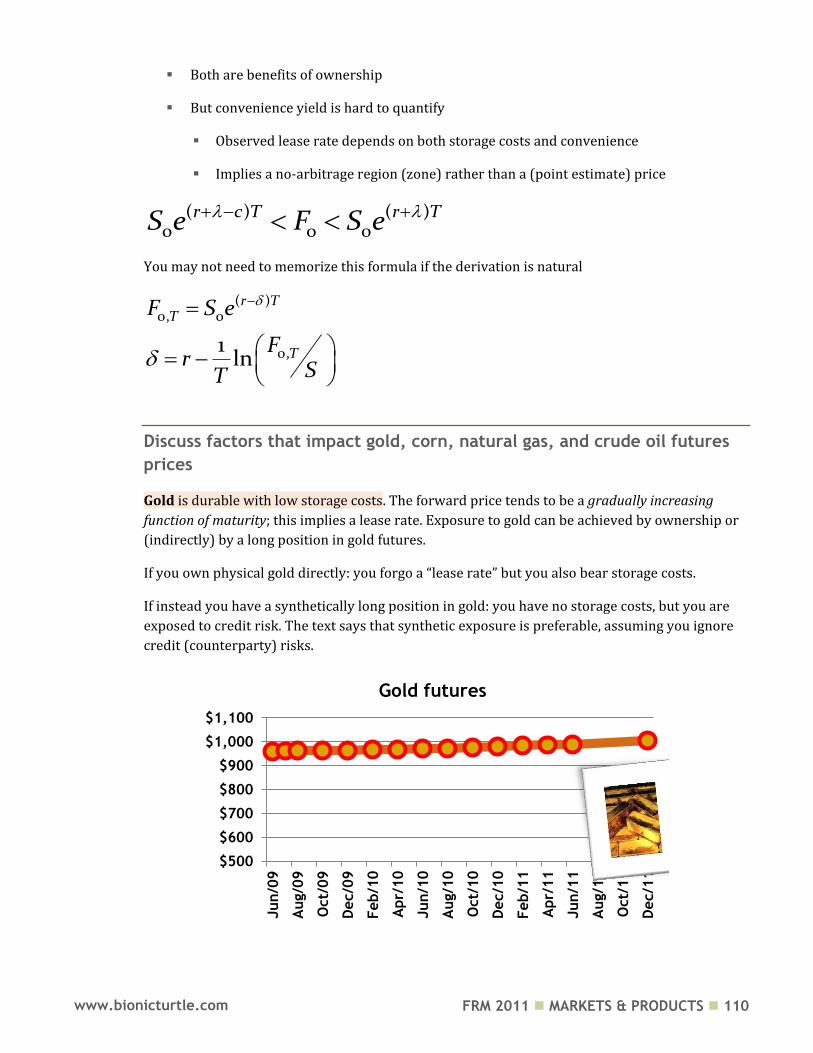
FRM 2011 MARKETS & PRODUCTS 110 www.bionicturtle.com
Both are benefits of ownership
But convenience yield is hard to quantify
Observed lease rate depends on both storage costs and convenience
Implies a no-arbitrage region (zone) rather than a (point estimate) price
( ) ( )0 0 0
r c T r TS e F S e
You may not need to memorize this formula if the derivation is natural
( )0, 0
0,1ln
r TT
T
F S e
Fr
ST
Discuss factors that impact gold, corn, natural gas, and crude oil futures
prices
Gold is durable with low storage costs. The forward price tends to be a gradually increasing
function of maturity; this implies a lease rate. Exposure to gold can be achieved by ownership or
(indirectly) by a long position in gold futures.
If you own physical gold directly: you forgo a “lease rate” but you also bear storage costs.
If instead you have a synthetically long position in gold: you have no storage costs, but you are
exposed to credit risk. The text says that synthetic exposure is preferable, assuming you ignore
credit (counterparty) risks.
$500
$600
$700
$800
$900
$1,000
$1,100
Jun/0
9
Aug/0
9
Oct/
09
Dec/0
9
Feb/1
0
Apr/
10
Jun/1
0
Aug/1
0
Oct/
10
Dec/1
0
Feb/1
1
Apr/
11
Jun/1
1
Aug/1
1
Oct/
11
Dec/1
1
Gold futures
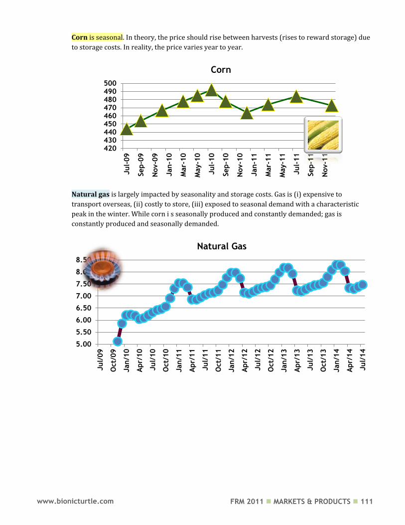
FRM 2011 MARKETS & PRODUCTS 111 www.bionicturtle.com
Corn is seasonal. In theory, the price should rise between harvests (rises to reward storage) due
to storage costs. In reality, the price varies year to year.
Natural gas is largely impacted by seasonality and storage costs. Gas is (i) expensive to
transport overseas, (ii) costly to store, (iii) exposed to seasonal demand with a characteristic
peak in the winter. While corn i s seasonally produced and constantly demanded; gas is
constantly produced and seasonally demanded.
420430440450460470480490500
Jul-
09
Sep-0
9
Nov-0
9
Jan-1
0
Mar-
10
May-1
0
Jul-
10
Sep-1
0
Nov-1
0
Jan-1
1
Mar-
11
May-1
1
Jul-
11
Sep-1
1
Nov-1
1
Corn
5.00
5.50
6.00
6.50
7.00
7.50
8.00
8.50
Jul/
09
Oct/
09
Jan/1
0
Apr/
10
Jul/
10
Oct/
10
Jan/1
1
Apr/
11
Jul/
11
Oct/
11
Jan/1
2
Apr/
12
Jul/
12
Oct/
12
Jan/1
3
Apr/
13
Jul/
13
Oct/
13
Jan/1
4
Apr/
14
Jul/
14
Natural Gas
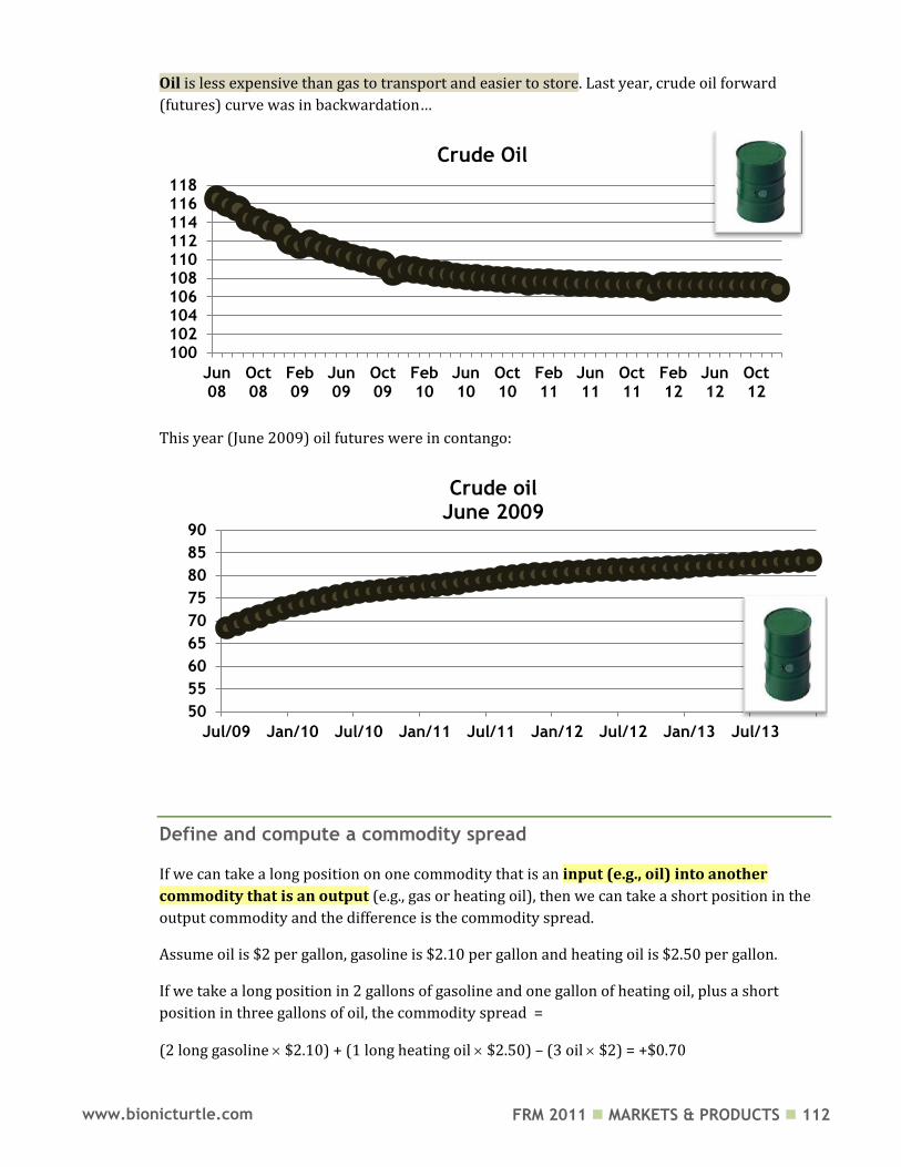
FRM 2011 MARKETS & PRODUCTS 112 www.bionicturtle.com
Oil is less expensive than gas to transport and easier to store. Last year, crude oil forward
(futures) curve was in backwardation…
This year (June 2009) oil futures were in contango:
Define and compute a commodity spread
If we can take a long position on one commodity that is an input (e.g., oil) into another
commodity that is an output (e.g., gas or heating oil), then we can take a short position in the
output commodity and the difference is the commodity spread.
Assume oil is $2 per gallon, gasoline is $2.10 per gallon and heating oil is $2.50 per gallon.
If we take a long position in 2 gallons of gasoline and one gallon of heating oil, plus a short
position in three gallons of oil, the commodity spread =
(2 long gasoline $2.10) + (1 long heating oil $2.50) – (3 oil $2) = +$0.70
100102104106108110112114116118
Jun08
Oct08
Feb09
Jun09
Oct09
Feb10
Jun10
Oct10
Feb11
Jun11
Oct11
Feb12
Jun12
Oct12
Crude Oil
50
55
60
65
70
75
80
85
90
Jul/09 Jan/10 Jul/10 Jan/11 Jul/11 Jan/12 Jul/12 Jan/13 Jul/13
Crude oil June 2009
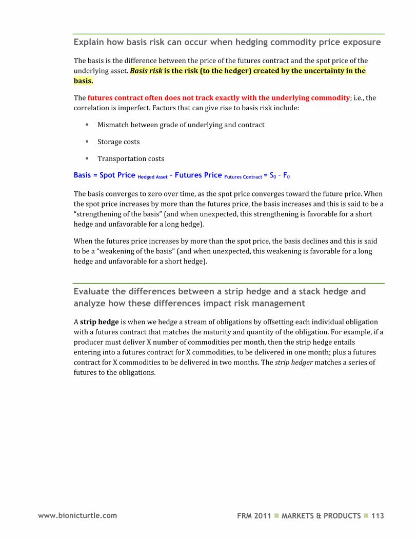
FRM 2011 MARKETS & PRODUCTS 113 www.bionicturtle.com
Explain how basis risk can occur when hedging commodity price exposure
The basis is the difference between the price of the futures contract and the spot price of the
underlying asset. Basis risk is the risk (to the hedger) created by the uncertainty in the
basis.
The futures contract often does not track exactly with the underlying commodity; i.e., the
correlation is imperfect. Factors that can give rise to basis risk include:
Mismatch between grade of underlying and contract
Storage costs
Transportation costs
Basis = Spot Price Hedged Asset – Futures Price Futures Contract = S0 – F0
The basis converges to zero over time, as the spot price converges toward the future price. When
the spot price increases by more than the futures price, the basis increases and this is said to be a
“strengthening of the basis” (and when unexpected, this strengthening is favorable for a short
hedge and unfavorable for a long hedge).
When the futures price increases by more than the spot price, the basis declines and this is said
to be a “weakening of the basis” (and when unexpected, this weakening is favorable for a long
hedge and unfavorable for a short hedge).
Evaluate the differences between a strip hedge and a stack hedge and
analyze how these differences impact risk management
A strip hedge is when we hedge a stream of obligations by offsetting each individual obligation
with a futures contract that matches the maturity and quantity of the obligation. For example, if a
producer must deliver X number of commodities per month, then the strip hedge entails
entering into a futures contract for X commodities, to be delivered in one month; plus a futures
contract for X commodities to be delivered in two months. The strip hedger matches a series of
futures to the obligations.
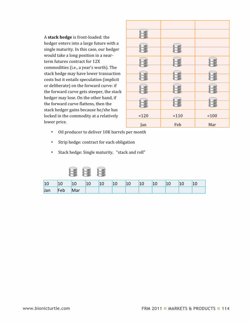
FRM 2011 MARKETS & PRODUCTS 114 www.bionicturtle.com
A stack hedge is front-loaded: the
hedger enters into a large future with a
single maturity. In this case, our hedger
would take a long position in a near-
term futures contract for 12X
commodities (i.e., a year’s worth). The
stack hedge may have lower transaction
costs but it entails speculation (implicit
or deliberate) on the forward curve: if
the forward curve gets steeper, the stack
hedger may lose. On the other hand, if
the forward curve flattens, then the
stack hedger gains because he/she has
locked in the commodity at a relatively
lower price.
Oil producer to deliver 10K barrels per month
Strip hedge: contract for each obligation
Stack hedge: Single maturity, “stack and roll”
10 10 10 10 10 10 10 10 10 10 10 10
Jan Feb Mar
<120 <110 <100
Jan Feb Mar
FRM 2011 MARKETS & PRODUCTS 115 www.bionicturtle.com
Geman, Chapter 1:
Fundamentals of
Commodity Spot
and Futures
Markets:
Instruments,
Exchanges and
Strategies
In this chapter…
Define ―bill of lading‖. Define the major risks involved with commodity spot transactions. Differentiate between ordinary and extraordinary transportation risks. Explain the major differences between spot, forward, and futures transactions,
markets, and contracts. Describe basic risk and its key components. Describe the basic characteristics and differences between hedgers,
speculators, and arbitrageurs. Describe an ―arbitrage portfolio‖ and explain the conditions for a market to be
arbitrage‐free. Define basis risk and the variance of the basis. Identify a commonly used measure for the effectiveness of hedging a spot
position with a futures contract; use this measure to compute and compare the effectiveness of alternative hedges.
Define and differentiate between an Exchange for Physical and agreement and an Alternative Delivery Procedure.
Describe one common measure of market depth.
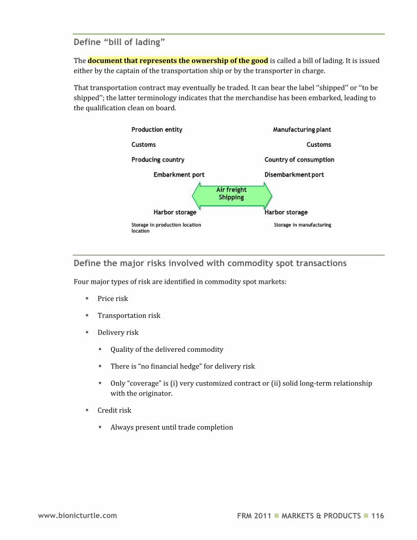
FRM 2011 MARKETS & PRODUCTS 116 www.bionicturtle.com
Define ―bill of lading‖
The document that represents the ownership of the good is called a bill of lading. It is issued
either by the captain of the transportation ship or by the transporter in charge.
That transportation contract may eventually be traded. It can bear the label ‘‘shipped’’ or ‘‘to be
shipped’’; the latter terminology indicates that the merchandise has been embarked, leading to
the qualification clean on board.
Define the major risks involved with commodity spot transactions
Four major types of risk are identified in commodity spot markets:
Price risk
Transportation risk
Delivery risk
Quality of the delivered commodity
There is “no financial hedge” for delivery risk
Only “coverage” is (i) very customized contract or (ii) solid long-term relationship
with the originator.
Credit risk
Always present until trade completion
FRM 2011 MARKETS & PRODUCTS 117 www.bionicturtle.com
Differentiate between ordinary and extraordinary transportation risks
The first category of risks concerns the deterioration, partial or total, of goods during
transportation. Two types of risks are usually recognized in this category:
Ordinary risks;
Extraordinary risks; wars, riots and strikes.
The expeditor of the goods or the FOB buyer directly holds the transportation risk, unless they
purchase an insurance contract to be covered.
Different companies specializing in freight insurance (such as the famous Lloyds of London)
propose various types of contracts. Major oil companies tend to self-insure deliver
transportation risk
Explain the major differences between spot, forward, and futures
transactions, markets, and contracts
Spot trading:
Any transaction where delivery either takes place immediately (which is rarely the case in
practice) or if there is a minimum lag, due to technical constraints, between the trade and
delivery.
Beyond a minimal lag, the trade becomes a forward agreement between the two parties and is
properly documented by a written contract.
Forward Contract
A forward contract is an agreement signed between two parties A and B at time 0, according to
which party A has the obligation of delivering at a fixed future date T an underlying asset and
party B the obligation of paying at that date an amount fixed at date 0, denoted FT
(0) and called
the forward price for date T for the asset.
( ) ( )TS T F T
Futures contracts analogous to forward contracts but key differences:
Standardized in terms of their characteristics (maturity, quantity of the underlying
commodity, quality or variety).
They are traded on an exchange, such as NYMEX or the IPE; hence, they carry no
counterparty risk since both the buyer and the seller of the Futures deal with the clearing
house of the exchange which is in principle fully trustworthy.
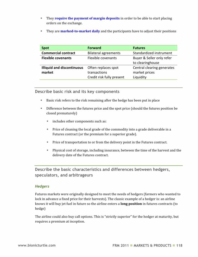
FRM 2011 MARKETS & PRODUCTS 118 www.bionicturtle.com
They require the payment of margin deposits in order to be able to start placing
orders on the exchange.
They are marked-to-market daily and the participants have to adjust their positions
Spot Forward Futures
Commercial contract Bilateral agreements Standardized instrument
Flexible covenants Flexible covenants Buyer & Seller only refer to clearinghouse
Illiquid and discontinuous market
Often replaces spot transactions
Central clearing generates market prices
Credit risk fully present Liquidity
Describe basic risk and its key components
Basic risk refers to the risk remaining after the hedge has been put in place
Difference between the futures price and the spot price (should the futures position be
closed prematurely)
includes other components such as:
Price of cleaning the local grade of the commodity into a grade deliverable in a
Futures contract (or the premium for a superior grade).
Price of transportation to or from the delivery point in the Futures contract.
Physical cost of storage, including insurance, between the time of the harvest and the
delivery date of the Futures contract.
Describe the basic characteristics and differences between hedgers,
speculators, and arbitrageurs
Hedgers
Futures markets were originally designed to meet the needs of hedgers (farmers who wanted to
lock in advance a fixed price for their harvests). The classic example of a hedger is: an airline
knows it will buy jet fuel in future so the airline enters a long position in futures contracts (to
hedge)
The airline could also buy call options. This is “strictly superior” for the hedger at maturity, but
requires a premium at inception.
FRM 2011 MARKETS & PRODUCTS 119 www.bionicturtle.com
Another classic example is a commodity producer who knows he/she will sell crop in future: the
producer enters into a short position in futures contracts in order to hedge.
Speculators
Speculators wish to get exposure to commodity price moves.
For example, Bank ABC (which has no ‘‘natural’’ exposure to the price of fuel) decides to take a
position (e.g., Futures contract on fuel, option on fuel). The position “expresses a view” on
subsequent moves in the fuel price.
Commodities are increasingly attractive to investors who view them as an alternative asset class
allowing them to improve return/risk profile
Futures are the obvious instrument:
Liquidity,
Low transaction costs on the exchange,
Absence of credit risk
Arbitragers
This is an important (but smaller in size) group of participants
An arbitrage is a riskless profit realized by simultaneously entering into several transactions
in two or more markets. Arbitrage opportunities are very desirable but not easy to uncover and
they do not persist.
Describe an ―arbitrage portfolio‖ and explain the conditions for a market
to be arbitrage‐free
If a portfolio requires a null investment and is riskless (there is no possible loss at the horizon
H), then its terminal value at date H has to be zero.
“No free lunch property:” if you start with no money and take no risk, your final wealth
will be zero.
The assumption of ‘‘riskless’’ is crucial
Note: In practice, traders searching for arbitrage opportunities are looking for ‘‘quasi-riskless’’
strategies generating profits.
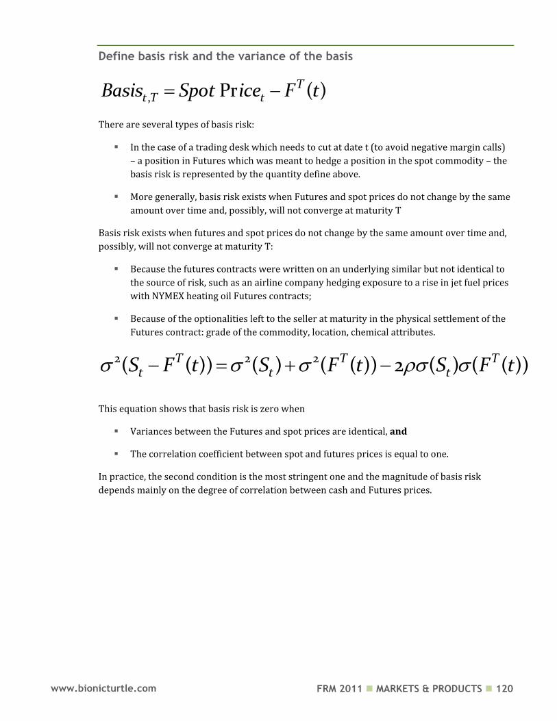
FRM 2011 MARKETS & PRODUCTS 120 www.bionicturtle.com
Define basis risk and the variance of the basis
, Pr ( )Tt T tBasis Spot ice F t
There are several types of basis risk:
In the case of a trading desk which needs to cut at date t (to avoid negative margin calls)
– a position in Futures which was meant to hedge a position in the spot commodity – the
basis risk is represented by the quantity define above.
More generally, basis risk exists when Futures and spot prices do not change by the same
amount over time and, possibly, will not converge at maturity T
Basis risk exists when futures and spot prices do not change by the same amount over time and,
possibly, will not converge at maturity T:
Because the futures contracts were written on an underlying similar but not identical to
the source of risk, such as an airline company hedging exposure to a rise in jet fuel prices
with NYMEX heating oil Futures contracts;
Because of the optionalities left to the seller at maturity in the physical settlement of the
Futures contract: grade of the commodity, location, chemical attributes.
2 2 2( ( )) ( ) ( ( )) 2 ( ) ( ( ))T T Tt t tS F t S F t S F t
This equation shows that basis risk is zero when
Variances between the Futures and spot prices are identical, and
The correlation coefficient between spot and futures prices is equal to one.
In practice, the second condition is the most stringent one and the magnitude of basis risk
depends mainly on the degree of correlation between cash and Futures prices.
FRM 2011 MARKETS & PRODUCTS 121 www.bionicturtle.com
Identify a commonly used measure for the effectiveness of hedging a spot
position with a futures contract; use this measure to compute and
compare the effectiveness of alternative hedges
The classical measure of the effectiveness of hedging a spot position with Futures contracts is
given by:
2
2
( )1
( )t
basish
S
The nearer (h) is to one, the better (more perfect) the hedge.
FRM 2011 MARKETS & PRODUCTS 122 www.bionicturtle.com
Define and differentiate between an Exchange for Physical and agreement
and an Alternative Delivery Procedure
Exchange For Physical
An EFP is an agreement between a party holding a long Futures position and a party with
an equal size short position to enter a bilateral contract specifying the terms of physical
delivery (location and price).
The two parties notify the clearing house of the quantity and price negotiated between
them and both futures positions are then terminated under the terms of the EFP.
In grain markets, this type of transaction is called ‘‘ex pit’’.
Alternative Delivery Procedure
An ADP is available to buyers and sellers who have been matched by the exchange subsequent to
the termination of trading in the spot month contract. If buyer and seller agree to achieve
delivery under terms different from those prescribed in the contract specifications, they may
proceed on that basis after submitting a notice of their intention to the exchange.
Describe one common measure of market depth
Liquidity may be measured by the size of the trade it takes to move the market.
Market depth may be measured by the time it takes for an order of a standard size to be
executed.
FRM 2011 MARKETS & PRODUCTS 123 www.bionicturtle.com
Cornett, Chapter
14: Foreign
Exchange Risk
In this chapter…
Calculate a financial institution’s overall foreign exchange exposure. Demonstrate how a financial institution could alter its net position exposure to
reduce foreign exchange risk. Calculate a financial institution’s potential dollar gain or loss exposure to a
particular currency. List and describe the different types of foreign exchange trading activities. Identify the sources of foreign exchange trading gains and losses. Calculate the potential gain or loss from a foreign currency denominated
investment. Explain balance‐sheet hedging with forwards. Describe how a non‐arbitrage assumption in the foreign exchange markets leads
to the interest rate parity theorem; use this theorem to calculate forward foreign exchange rates.
Explain why diversification in multicurrency asset‐liability positions could reduce portfolio risk.
Describe the relationship between nominal and real interest rates.
Foreign Exchange Rates
Direct quote (US$ Equivalent)
U.S. dollars per one unit of foreign currency
0.9079 USD / CAD
Indirect quote (Currency per US$)
Foreign currency per one US dollar
1.1015 CAD / $USD
FRM 2011 MARKETS & PRODUCTS 124 www.bionicturtle.com
Calculate a financial institution’s overall foreign exchange exposure.
Demonstrate how a financial institution could alter its net position
exposure to reduce foreign exchange risk
Net exposurei = (FX assetsi - FX liabilitiesi) + (FX boughti - FX soldi) = Net foreign assetsi + Net FX
boughti
i = Ith currency
Positive net exposure: net long a currency
Negative net exposure: net short a currency
To reduce its foreign currency exposure:
Bank can match its foreign currency assets to its liabilities
Bank can match buys and sells in trading book
Financial holding companies can aggregate their foreign exchange exposure; e.g., under one
umbrella, commercial bank, insurance company, pension fund
Calculate a financial institution’s potential dollar gain or loss exposure to
a particular currency
The potential size of a bank’s FX exposure given by:
Dollar loss/gain in currency i =
Net exposure in foreign currency I measured in US dollars
Shock (volatility) to the $/foreign currency I exchange rate
List and describe the different types of foreign exchange trading activities
A bank’s position in the FX markets generally reflects four (4) trading activities. The
purchase/sale of foreign currencies …
1. To allow customers to participate in international commercial trade transactions
2. To allow customers to take positions in foreign investments (real or financial assets)
3. For hedging purposes—i.e., to offset currency exposure
4. For speculative purposes
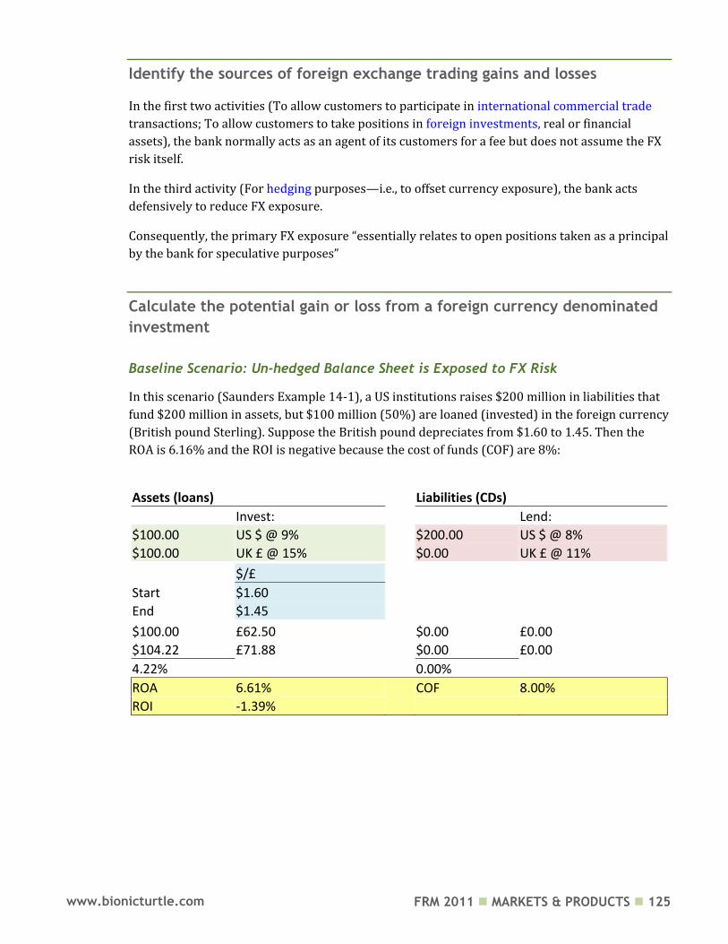
FRM 2011 MARKETS & PRODUCTS 125 www.bionicturtle.com
Identify the sources of foreign exchange trading gains and losses
In the first two activities (To allow customers to participate in international commercial trade
transactions; To allow customers to take positions in foreign investments, real or financial
assets), the bank normally acts as an agent of its customers for a fee but does not assume the FX
risk itself.
In the third activity (For hedging purposes—i.e., to offset currency exposure), the bank acts
defensively to reduce FX exposure.
Consequently, the primary FX exposure “essentially relates to open positions taken as a principal
by the bank for speculative purposes”
Calculate the potential gain or loss from a foreign currency denominated
investment
Baseline Scenario: Un-hedged Balance Sheet is Exposed to FX Risk
In this scenario (Saunders Example 14-1), a US institutions raises $200 million in liabilities that
fund $200 million in assets, but $100 million (50%) are loaned (invested) in the foreign currency
(British pound Sterling). Suppose the British pound depreciates from $1.60 to 1.45. Then the
ROA is 6.16% and the ROI is negative because the cost of funds (COF) are 8%:
Assets (loans)
Liabilities (CDs)
Invest:
Lend:
$100.00 US $ @ 9%
$200.00 US $ @ 8%
$100.00 UK £ @ 15%
$0.00 UK £ @ 11%
$/£
Start $1.60
End $1.45
$100.00 £62.50
$0.00 £0.00
$104.22 £71.88
$0.00 £0.00
4.22%
0.00%
ROA 6.61% COF 8.00%
ROI -1.39%
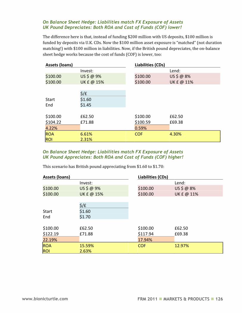
FRM 2011 MARKETS & PRODUCTS 126 www.bionicturtle.com
On Balance Sheet Hedge: Liabilities match FX Exposure of Assets UK Pound Depreciates: Both ROA and Cost of Funds (COF) lower!
The difference here is that, instead of funding $200 million with US deposits, $100 million is
funded by deposits via U.K. CDs. Now the $100 million asset exposure is “matched” (not duration
matching!) with $100 million in liabilities. Now, if the British pound depreciates, the on-balance
sheet hedge works because the cost of funds (COF) is lower, too:
On Balance Sheet Hedge: Liabilities match FX Exposure of Assets UK Pound Appreciates: Both ROA and Cost of Funds (COF) higher!
This scenario has British pound appreciating from $1.60 to $1.70:
Assets (loans)
Liabilities (CDs) Liabilities (CDs)
Invest:
Lend: $100.00 US $ @ 9%
$100.00 US $ @ 8%
$100.00 UK £ @ 15%
$100.00 UK £ @ 11%
$/£
Start $1.60
End $1.45
$100.00 £62.50
$100.00 £62.50 $104.22 £71.88
$100.59 £69.38
4.22%
0.59%
ROA 6.61% COF 4.30% ROI 2.31%
Assets (loans)
Liabilities (CDs)
Invest:
Lend:
$100.00 US $ @ 9%
$100.00 US $ @ 8% $100.00 UK £ @ 15%
$100.00 UK £ @ 11%
$/£
Start $1.60
End $1.70
$100.00 £62.50
$100.00 £62.50 $122.19 £71.88
$117.94 £69.38
22.19%
17.94%
ROA 15.59%
COF 12.97%
ROI 2.63%
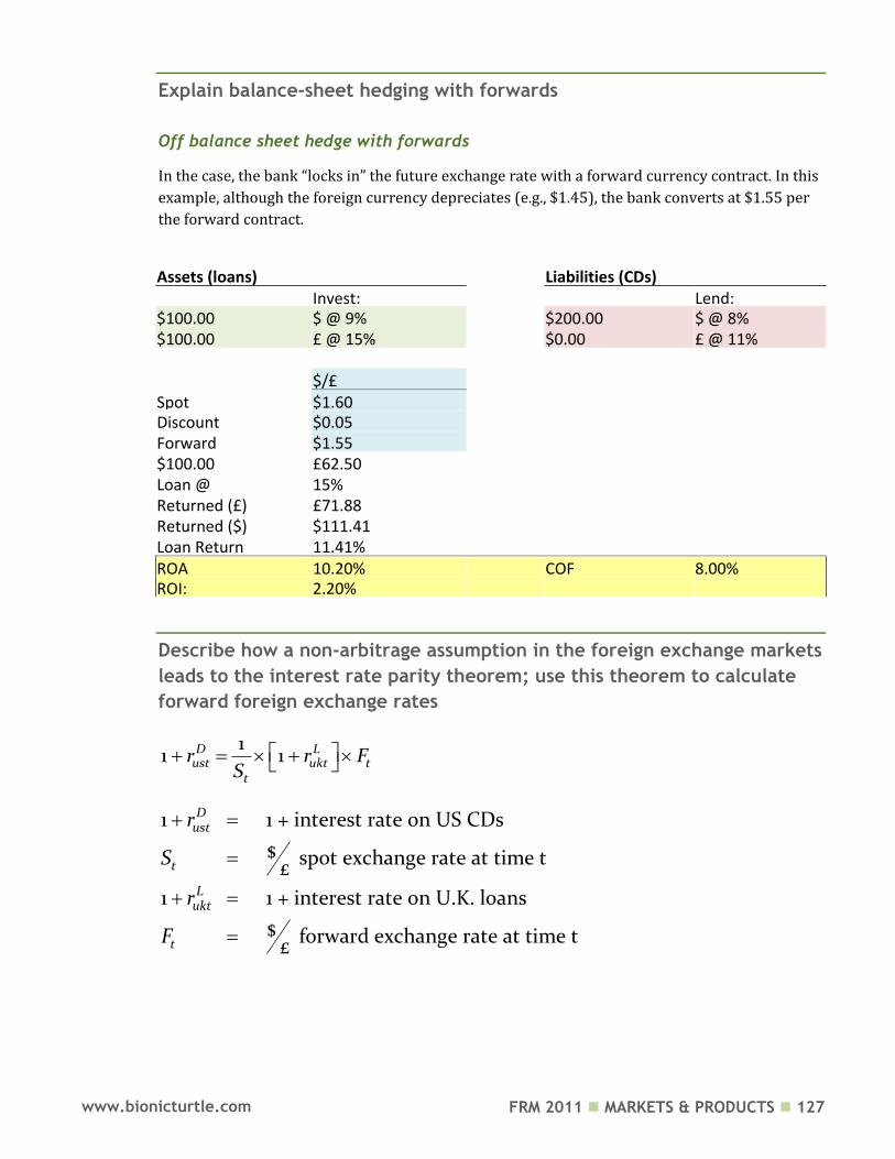
FRM 2011 MARKETS & PRODUCTS 127 www.bionicturtle.com
Explain balance‐sheet hedging with forwards
Off balance sheet hedge with forwards
In the case, the bank “locks in” the future exchange rate with a forward currency contract. In this
example, although the foreign currency depreciates (e.g., $1.45), the bank converts at $1.55 per
the forward contract.
Describe how a non‐arbitrage assumption in the foreign exchange markets
leads to the interest rate parity theorem; use this theorem to calculate
forward foreign exchange rates
11 1D L
ust ukt tt
r r FS
1 1 + interest rate on US CDs
$ spot exchange rate at time t£
1 1 + interest rate on U.K. loans
$ forward exchange rate at time t£
Dust
t
Lukt
t
r
S
r
F
Assets (loans)
Liabilities (CDs)
Invest:
Lend:
$100.00 $ @ 9%
$200.00 $ @ 8% $100.00 £ @ 15%
$0.00 £ @ 11%
$/£
Spot $1.60 Discount $0.05 Forward $1.55 $100.00 £62.50 Loan @ 15% Returned (£) £71.88 Returned ($) $111.41 Loan Return 11.41% ROA 10.20% COF 8.00%
ROI: 2.20%
FRM 2011 MARKETS & PRODUCTS 128 www.bionicturtle.com
Explain why diversification in multicurrency asset‐liability positions could
reduce portfolio risk
To the degree that domestic and foreign interest rates (or stock returns) are not perfectly
correlated, potential gains from asset-liability portfolio diversification can offset risk of asset-
liability currency mismatch.
Describe the relationship between nominal and real interest rates
Nominal interest rate = real interest rate + expected inflation rate
ei i ir rr i
The nominal interest rate in country The real interest rate in country The expected one-period inflation rate in country
i
iei
r irr ii i
FRM 2011 MARKETS & PRODUCTS 129 www.bionicturtle.com
Cornett, Appendix
15A: Mechanisms
for Dealing with
Sovereign Risk
Exposure
In this chapter…
Define four alternative mechanisms for dealing with problem sovereign credits. Describe the major incentives and disincentives for participants in a debt‐for‐
equity swap, including tax considerations and the impact of regulatory constraints.
Describe the advantages and disadvantages of multiyear restructuring agreements.
Define the major elements of a multiyear restructuring agreement, including concessionality.
Describe the major benefits and costs of loan sales. Describe the major benefits and costs of bond‐for‐loan swaps.
Sovereign versus credit risk
Sovereign risk: foreign government may default or fail to honor commitments
In addition to credit quality of firm, two challenges
Even if unlikely, it is possible that the foreign government blocks repayments made in
dollars (e.g., if their reserve position deteriorates)
Unlike the United States, where the lender can seek a legal remedy in bankruptcy court,
there is no international bankruptcy court.
Two-step lending decision (to foreign company):
Lenders must assess the underlying credit quality of the borrower, as it would do for a
normal domestic loan, including setting an appropriate credit risk premium or credit
limits
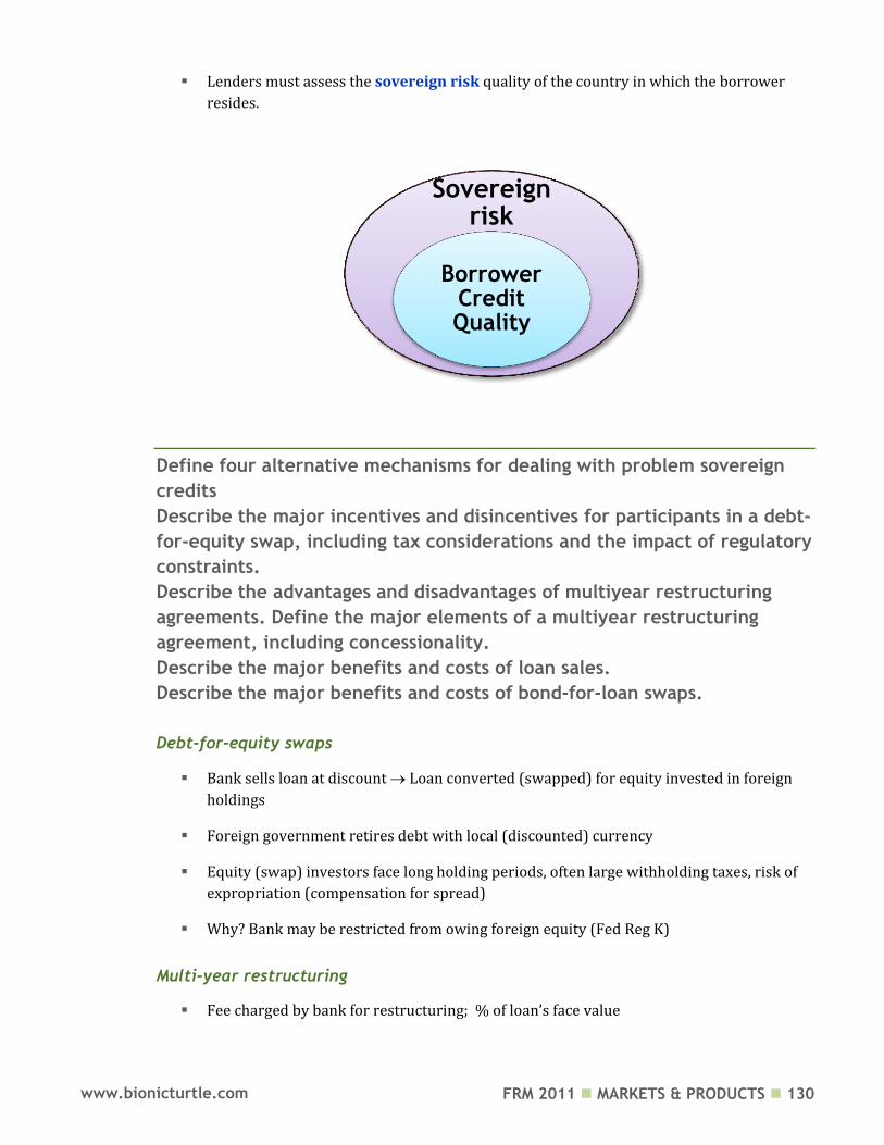
FRM 2011 MARKETS & PRODUCTS 130 www.bionicturtle.com
Lenders must assess the sovereign risk quality of the country in which the borrower
resides.
Define four alternative mechanisms for dealing with problem sovereign
credits
Describe the major incentives and disincentives for participants in a debt‐
for‐equity swap, including tax considerations and the impact of regulatory
constraints.
Describe the advantages and disadvantages of multiyear restructuring
agreements. Define the major elements of a multiyear restructuring
agreement, including concessionality.
Describe the major benefits and costs of loan sales.
Describe the major benefits and costs of bond‐for‐loan swaps.
Debt-for-equity swaps
Bank sells loan at discount Loan converted (swapped) for equity invested in foreign
holdings
Foreign government retires debt with local (discounted) currency
Equity (swap) investors face long holding periods, often large withholding taxes, risk of
expropriation (compensation for spread)
Why? Bank may be restricted from owing foreign equity (Fed Reg K)
Multi-year restructuring
Fee charged by bank for restructuring; % of loan’s face value
Sovereign risk
Borrower Credit Quality
FRM 2011 MARKETS & PRODUCTS 131 www.bionicturtle.com
Interest rate on new loan
Grace period
Maturity extension
Option and guarantee features
LDC Loan Sale
Removal from balance sheet
Signals B/S strength
Government share loss due to tax loss write-off
Loss itself
Bonds-for-loan swaps (Brady bonds)
Becomes highly liquid instrument
But typically at discount
But typically with longer maturity
Posting U.S. debt as collateral can be expensive for LDC
FRM 2011 MARKETS & PRODUCTS 132 www.bionicturtle.com
Fabozzi, Chapter
13: Corporate
Bonds
In this chapter…
Describe a bond indenture and explain the role of the corporate trustee. Explain a bond’s maturity date and how it impacts bond retirements. Describe the main types of interest payment classifications. Describe zero‐coupon bonds, the relationship between original‐issue‐discount
and reinvestment risk, and the treatment of zeroes in bankruptcy. Describe the various security types relevant for corporate bonds, including:
Mortgage bonds Collateral trust bonds Equipment trust certificates Debenture bonds (including subordinated and convertible debentures) Guaranteed bonds
Describe the mechanisms by which corporate bonds can be retired before maturity, including: Call provisions Sinking‐fund provisions Maintenance and replacement funds Tender offers
Describe, and differentiate between credit default risk and credit spread risk. Describe event risk and what may cause it in corporate bonds. Define high‐yield bonds, describe types of high‐yield bond issuers, and some of
the payment features peculiar to high yield bonds. Define and differentiate between an issuer default rate and a dollar default
rate. Define recovery rates and describe the relationship between recovery rates and
seniority.
Describe a bond indenture and explain the role of the corporate trustee
Bond indenture
The contract that contains corporate bond issuer promises and investors’ rights. The indenture
is made out to corporate trustee, who represents bondholders’ interests.
FRM 2011 MARKETS & PRODUCTS 133 www.bionicturtle.com
Corporate trustee
Third party to the contract. Acts in fiduciary capacity for investors
Is a bank or trust company with a corporate trust department and officers who are experts in
performing trustee functions.
Trustee authenticates the bonds issued.
Is the watchdog for the bondholders: ensures that issuer complies with all the covenants of the
indenture.
These covenants are many and technical, and they must be watched during the entire period that
a bond issue is outstanding.
Corporate Bonds
The five broad categories of corporate bonds sold in the United States based on the type of issuer
are
Public utilities,
Transportations,
Industrials,
Banks and finance companies; and
International or Yankee issues.
Explain a bond’s maturity date and how it impacts bond retirements
Bond’s maturity: date on which the issuer’s obligation to satisfy the terms of the indenture is
fulfilled.
Principal is repaid with any premium and accrued interest that may be due.
However, many issues can be retired prior to maturity.
FRM 2011 MARKETS & PRODUCTS 134 www.bionicturtle.com
Describe the main types of interest payment classifications
The three main interest payment classifications of domestically issued corporate bonds are
Straight-coupon bonds,
Zero-coupon bonds, and
Floating-rate, or variable-rate, bonds.
Describe zero‐coupon bonds, the relationship between original‐issue‐
discount and reinvestment risk, and the treatment of zeroes in
bankruptcy
Zero-coupon bonds: bonds without coupons or an interest rate. Zero-coupon
bonds pay only the principal portion at some future date.
Zero-coupon bonds are issued at discounts to par; the difference is the return to the
bondholder.
The difference between the face amount and the offering price when first issued is called
the original-issue discount (OID).
The rate of return depends on the amount of the discount and the period over which it
accretes
Zero coupon bond
A zero-coupon bond eliminates reinvestment risk (shifting all of the risk to interest rate risk;
e.g., duration) because there is no coupon to reinvest. A zero is considered beneficial in
declining-interest-rate markets, but not when interest rates are rising.
Recall Tuckman: a bond investor faces a a tradeoff between reinvestment risk
(the reinvestment of coupons) and interest rate risk.
Investors tend to find zeros less attractive in lower-interest-rate markets
Compounding is not as meaningful when rates are lower (compared to higher rates).
Also, lower the rates are, the more likely it is that they will rise again, making a zero-coupon
investment worth less in the eyes of potential holders.
FRM 2011 MARKETS & PRODUCTS 135 www.bionicturtle.com
Treatment of zeroes in bankruptcy
In bankruptcy, zero-coupon bond creditor claim original offering price
plus accrued and unpaid interest, but not the principal amount of
$1,000.
Zero-coupon bonds are sold at (deep) discounts: liability of the issuer at
maturity may be substantial.
There are no sinking funds on most of these issues.
The potentially large balloon repayment creates a cause for concern among investors. Thus it is
most important to invest in higher-quality issues so as to reduce the risk of a potential problem.
Describe the various security types relevant for corporate bonds,
including:
Mortgage bonds
A mortgage bond grants bondholders a first-mortgage lien on
substantially all its properties.
Issuer is able to borrow at a lower interest rate than unsecured debt
A lien is a legal right to sell mortgaged property to satisfy unpaid
obligations to bondholders.
Foreclosure and sale of mortgaged property are not typical. In default, typically a financial
reorganization; provisions made for settlement of the debt to bondholders
But mortgage lien gives bondholders a very strong bargaining position relative to other creditors
in determining the terms of a reorganization.
Collateral trust bonds
When companies cannot pledge fixed assets or other real property, instead they pledge
securities of other companies
To satisfy the desire of bondholders for security, they pledge stocks, notes,
bonds, or whatever other kinds of obligations they own.
If they are holding companies, the other companies may be their
subsidiaries.
These assets are termed collateral (or personal property), and bonds secured by such assets are
collateral trust bonds.
FRM 2011 MARKETS & PRODUCTS 136 www.bionicturtle.com
Equipment trust certificates
Although railroads have issued the largest amount of equipment trust certificates, airlines also
have used this form of financing. The legal arrangement is one that vests legal title to railway
equipment in a trustee, which is better from the standpoint of investors than a first-mortgage
lien on property. A railway company orders some cars and locomotives from a manufacturer.
When the job is finished, the manufacturer transfers the legal title to the equipment to a trustee.
The trustee leases it to the railroad that ordered it and at the same time sells equipment trust
certificates (ETCs) in an amount equal to a large percentage of the purchase price, normally
80%. Money from sale of certificates is paid to the manufacturer.
Debenture bonds (including subordinated and convertible debentures)
Unsecured bonds are called debentures.
With the exception of the utilities and structured products, nearly all other corporate bonds
issued are unsecured.
Debenture bondholders do have the claim of general creditors on all assets of the issuer not
pledged specifically to secure other debt.
Subordinated debenture bonds: issue ranks after secured debt, after debenture bonds, and
often after some general creditors in its claim on assets and earnings. Owners of this bond “stand
last in line”.
Because subordinated debentures are weaker in their claim on assets, issuers must offer a
higher rate of interest…unless they also offer some special inducement to buy the bonds.
The inducement can be an option to convert bonds into stock of the issuer at the discretion of
bondholders.
This conversion privilege also may be included in the provisions of debentures that are not
subordinated.
The bonds may be convertible into the common stock of a corporation other than that of the
issuer. Such issues are called exchangeable bonds. There are also issues indexed to a
commodity’s price or its cash equivalent at the time of maturity or redemption.
Guaranteed bonds
Guaranteed bonds: a corporation may guarantee the bonds of another corporation.
The guarantee, however, does not mean that these obligations are free of default risk. The safety
of a guaranteed bond depends on the financial capability of the guarantor to satisfy the terms of
the guarantee, as well as the financial capability of the issuer. The terms of the guarantee may
call for the guarantor to guarantee the payment of interest and/or principal repayment
FRM 2011 MARKETS & PRODUCTS 137 www.bionicturtle.com
Describe the mechanisms by which corporate bonds can be retired before
maturity, including:
Retiring bonds before maturity
Call and refunding provisions
Fixed-price call provision
Make-whole call provision
Sinking-fund provision
Maintenance and replacement funds
Redemption through sale of assets
Tender offers
Call provisions
Fixed price
Bond issuer has the option to buy back some or all of the bond issue prior to maturity at a fixed
price (“call price”).
Call prices generally start at a substantial premium over par and decline toward par over time; in
the final years of a bond’s life, the call price is usually par.
Make-whole
Call price is calculated as the present value of the bond’s remaining cash flows subject to a floor
price equal to par value. The discount rate used to determine the present value is the yield on a
comparable maturity
Call provision: Corporate bonds that contains an embedded option that gives the issuer the
right to buy the bonds back at a fixed price prior to maturity, either in whole or in part.
The ability to retire debt before its scheduled maturity date is a valuable option for which
bondholders will demand compensation ex-ante.
Ceteris paribus, bondholders will pay a lower price for a callable bond than an otherwise
identical option-free (i.e., straight) bond.
The difference between the price of an option-free bond and the callable bond is the value of the
embedded call option
FRM 2011 MARKETS & PRODUCTS 138 www.bionicturtle.com
Sinking‐fund provisions
Money applied periodically to redemption of bonds before maturity. Two advantages from the
bondholder’s perspective:
Default risk is reduced
If bond prices decline as a result of an increase in interest rates, price support may be
provided by the issuer or its fiscal agent because it must enter the market on the buy side
in order to satisfy the sinking-fund requirement.
Disadvantage is the bonds may be called at the special sinking-fund call price at a time when
interest rates are lower than rates prevailing at time of issuance.
Maintenance and replacement funds
Maintenance and replacement fund (M&R) provisions first appeared in bond indentures of
electric utilities subject to regulation by the Securities and Exchange Commission (SEC) under
the Public Holding Company Act of 1940. It remained in the indentures even when most of the
utilities were no longer subject to regulation under the act. The original motivation for their
inclusion is straightforward. Property is subject to economic depreciation, and the replacement
fund ostensibly helps to maintain the integrity of the property securing the bonds. An M&R
differs from a sinking fund in that the M&R only helps to maintain the value of the security
backing the debt, whereas a sinking fund is designed to improve the security backing the debt.
Although it is more complex, it is similar in spirit to a provision in a home mortgage requiring
the homeowner to maintain the home in good repair.
Tender offers
At any time a firm may execute a tender offer and announce its desire to buy back specified debt
issues.
Firms employ tender offers to eliminate restrictive covenants or to refund debt.
Usually the tender offer is for “any and all” of the targeted issue, but it also can be for afixed
dollar amount that is less than the outstanding face value.
An offering circular is sent to the bondholders of record stating the price the firm is willing to
pay and the window of time during which bondholders can sell their bonds back to the firm.
FRM 2011 MARKETS & PRODUCTS 139 www.bionicturtle.com
Describe, and differentiate between credit default risk and credit spread
risk
Credit default risk
Any bond investment carries with it the uncertainty as to whether the issuer will make timely
payments of interest and principal as prescribed by the bond’s indenture.
Credit default risk is the risk that a bond issuer will be unable to meet its financial obligations.
The credit spread is the difference between a corporate bond’s yield and the yield on a
comparable-maturity benchmark Treasury security.
What explains the difference?
The difference in yields is due primarily to the corporate bond’s exposure to credit risk. But not
only this!
The risk profile of corporate bonds differs from Treasuries on other dimensions; corporate
bonds are less liquid and may have embedded options.
Credit-spread risk is the risk of financial loss resulting from changes in the level of credit spreads
used in the marking-to-market of a fixed income product. Credit spreads driven by:
Macroeconomic forces include such things as the level and slope of the Treasury yield curve,
the business cycle, and consumer confidence
Issue-specific factors include the corporation’s financial position and the future prospects of
the firm and its industry.
Describe event risk and what may cause it in corporate bonds
Event risk is the risk that a transaction (or corporate event) will devalue bondholder’s position.
Restructurings, recapitalizations, mergers, acquisition, leveraged buyouts, and share
repurchases often cause substantial changes in a corporation’s capital structure, greatly
increased leverage and decreased equity.
Event risk has caused some companies to include other special debt- retirement features in their
indentures.
An example is the maintenance of net worth clause included in the indentures of some lower-
rated bond issues.
FRM 2011 MARKETS & PRODUCTS 140 www.bionicturtle.com
Define high‐yield bonds, describe types of high‐yield bond issuers, and
some of the payment features peculiar to high yield bonds
High-yield bonds are those rated below investment grade by the ratings agencies.
Also known as junk bonds.
Types
Original Issuers
Fallen Angels
Restructurings and Leverage Buyouts
Three types of deferred-coupon structures:
1. Deferred-interest bonds,
2. Step-up bonds, and
3. Payment-in-kind bonds.
Define and differentiate between an issuer default rate and a dollar
default rate
Issuer default rate
Number of issuers that default divided by total number of issuers
Gives no recognition to amount defaulted nor amount of issuance
Dollar default rate
Par value of all defaulted bonds divided by total par value of bonds outstanding during the year
(Altman uses this method)
Average annual default rate
Cumulative $ value of all defaulted bonds ÷ Cumulative $ value of all issuance
average number of years outstanding
Cumulate default rate
Cumulative $ value of all defaulted bonds ÷ Cumulative $ value of all issuance
FRM 2011 MARKETS & PRODUCTS 141 www.bionicturtle.com
Define recovery rates and describe the relationship between recovery
rates and seniority
Measuring the amount recovered is non-trivial
The final distribution to claimants may consist of cash and securities.
Often it is difficult to track what was received and then determine the present value of any
noncash payments received.
Moody’s uses the trading price at the time of default as a proxy for the amount recovered.
The recovery rate is the trading price at that time divided by the par value.
Moody’s found that the recovery rate was 38% for all bonds.
While default rates are the same regardless of the level of seniority, recovery rates differ. The
study found that the higher the level of seniority, the greater is the recovery rate.