Frito-Lay - Supply Chain Impact Analysis

CALIFORNIA POLYTECHNIC STATE UNIVERSITY

Frito-Lay – Supply Chain

Impact Analysis

A Senior Project submitted in partial fulfillment of

the requirements for the degree of Bachelor of

Science in Industrial Engineering

Kerri Blosch, Vincent Phua, Jeffrey Silva

3/20/2015

An examination into the effects of cannibalization when a store selling Frito Lay products opens or closes

in an area. Short-term effects were found between similar stores but long-term effects were inconclusive.

1

Executive Summary

The snack food company Frito-Lay relies on Route Sales Representatives (RSRs) to stock and

maintain shelves of snack foods in every store. Frito-Lay currently does not have a system which

can accurately predict cannibalization, or the effects of a store opening or closing on other stores

of the same chain in the area. The goal is to sort through 1900 stores in a given metropolitan area

to see the effects of cannibalization. In order to tackle the problem, a Microsoft Access program

was created to filter stores based on location or whether the store was open for the full three-year

duration or not.

The analysis of an opening or closing store is divided between the long-term and short-term

effects. An examination of the long-term effects begins by focusing on eliminating seasonal and

yearly trends. Seasonal trends are deemed to be insignificant due to the lack of a dominant

oscillation within the year. Next, yearly trends are eliminated by performing an individual

regression analysis between the introduced store and a nearby store and tracking the sales

changes on control charts. A scatterplot is created using the distance between the neighboring

store and the introduced store versus the sales changes. A trend line is fitted to the data, but little

correlation can be seen. The long-term effects are inconclusive because the model does not

incorporate different factors that could affect sales numbers.

The short-term effects were analyzed using a combination of control charts, percentage changes,

and sales averages before and after the store’s introduction. The most statistically significant

interactions were same-store cannibalization for mass merchandisers and supermarkets. This

supports the already-standing practices by Frito-Lay.

2

Contents

Executive Summary .................................................................................................................................... 1

Introduction ................................................................................................................................................. 4

Background ................................................................................................................................................. 5

Bullwhip Effect .......................................................................................................................................... 5

Vendor-Managed Inventory (VMI) ........................................................................................................... 5

Sales Territories ........................................................................................................................................ 5

Cannibalization ......................................................................................................................................... 6

Supply Chain ............................................................................................................................................. 6

Literature Review ....................................................................................................................................... 7

Measuring Cannibalization ...................................................................................................................... 7

Gains Loss Analysis .................................................................................................................................. 7

Duplication of Purchase Tables ................................................................................................................ 7

Data Mining ............................................................................................................................................ 11

Demand Forecasting ............................................................................................................................... 13

Need for Forecasting Model ............................................................................................................... 13

Forecasting Model .............................................................................................................................. 14

Variables Which Affect Sales of a Chain Retail Store in a Shopping Mall ............................................. 15

Regression Analysis ................................................................................................................................ 15

Integer Programming .............................................................................................................................. 16

Design ......................................................................................................................................................... 18

Provided Data ......................................................................................................................................... 18

Organizing Data ..................................................................................................................................... 19

Intervention Analysis .............................................................................................................................. 19

Long-term Trends.................................................................................................................................... 20

Discussion .................................................................................................................................................. 24

Limitations .............................................................................................................................................. 27

Conclusions ................................................................................................................................................ 28

Works Cited ............................................................................................................................................... 29

Appendix .................................................................................................................................................... 30

3

Table of Figures

Figure 1: Distance Plotted Against Sales Growth .............................................................................10

Figure 2: CRISP-DM Model .........................................................................................................12

Figure 3: Integer Programming County Map ...................................................................................17

Figure 4 - Histogram of Mass Merchandisers' Sales in 2012 .............................................................21

Figure 5: I-MR Chart of Impacted Mass Merchandiser Sales from Introduction of Supermarket ............22

Figure 6: Scatterplot of Distance Versus Deviation in Sales for Mass Merchandisers to Convenience

Stores .........................................................................................................................................25

Table 1: List of Store Types Provided .......................................................................................... 18

Table 2: Results of Closing Store (1-Mile Radius) ....................................................................... 25

Table 3: Results of Closing Store (5-Mile Radius) ....................................................................... 26

Table 4: Results of Opening Store (1-Mile Radius) ..................................................................... 26

Table 5: Results of Opening Store (5-Mile Radius) ..................................................................... 26

4

Introduction

An iconic brand like Frito Lay has many loyal customers throughout the world who understand

how quality of raw materials, packaging, distribution, and marketing combine to make a superior

end-product. Through their “seed to shelf” supply chain management technique, where only Frito

Lay team members handle the product until the consumer purchases it, the snack food company

dominates the market with many of their products. Sales and marketing are keys for success.

With consumer competitions like “Do Us a Flavor,” where actual customers design their dream

chip for a chance to win a million dollars, sales increase along with brand recognition. Frito Lay

utilizes the experience, intelligence, and dedication of their team to excel with core products, and

also expand into new product markets.

In the retail industry, specifically for food vendors, it can be difficult to accurately forecast the

effect of the closing of a store. Similarly, it can be difficult to approximate the impact of a new

store being introduced into a sale zone. For a company like Frito Lay, which manages a breadth

of products that are sold at many convenience stores and supermarkets, developing a system that

is capable of forecasting the effects of changes in certain markets would be beneficial. The

accuracy of their forecasting system directly affects their employees’ lives, especially the Route

Sales Representatives (RSRs). The main job function of an RSR is to deliver Frito Lay products

to stores while visually managing inventory levels. An inaccurate forecast means the possibility

of an RSR losing income, which is tied to the amount of product they are able to distribute.

The objectives of this report are as follows:

● Employ data mining to extract data according to metrics of interest

● Utilize data to construct forecasting model/tool

● Distinguish the different solutions for forecasting methods based on store type

In order to accomplish these objectives, case studies on topics like sales territories, forecasting,

cannibalization, data mining, and operations research will be utilized to devise a solution. The

remainder of the report is broken up into the following sections: background, literature review,

and methodology. The literature review will encompass the analysis of case studies on topics

such as cannibalization, data mining, forecasting and operations research.

5

Background

It is essential to understand the structure of Frito Lay’s sales in order to create a forecasting tool.

Frito Lay employs vendor-managed inventory (VMI), which is driven by their RSRs. This means

that the Sales Representatives have a certain route in which they are responsible for stocking

product, displaying product in an attractive manner, and determining order sales for the next

visit. The buyer (a particular type of store) does not order inventory for the store; rather, Frito

Lay holds that responsibility.

Competition is fierce in the retail store industry all over the world, which causes chains to open

and close stores constantly. Inevitably, markets with a store arriving or departing have a

redistribution of demand driven by several factors such as variety of product, prices, and travel

cost, among others. The topic of demand redistribution will be examined further in the literature

review and the body of the following paper. Below are some concepts that provide background

knowledge for the ensuing report.

Bullwhip Effect

In supply chains with many links, transmission of information can be delayed, disrupted, or

amplified due to each link’s attempt to create a buffer. When demand swings occur, the delay in

information sharing creates huge swings in inventory levels and order sizes. Links further down

the supply chain see a larger bullwhip effect, similar to the way the end of an actual whip

experiences larger range of motion than the section near the handle.

Vendor-Managed Inventory (VMI)

Vendor-Managed Inventory is a distribution operating system by which the supplier/vendor

monitors and manages the inventory at a distributor/retailer. This method helps to reduce the

Bullwhip effect by reducing the amount of times that information is passed from supplier to

distributor, and is very popular in the grocery sector (Nachiappan, 2005).

Sales Territories

Maintaining a balanced network of sales zones is important for Frito Lay. Sales zones with a

greater store count suffer from under-utilization of potentially profitable customers. Sales

Representatives in those zones will generally focus their time on easy accounts and may not

extend their focus to stores with smaller sales generation. On the other hand, Sales

6

Representatives in zones with lower prospects suffer from a decrease in morale, which can lead

to higher turnovers. These Sales Representatives will also spend a disproportionate amount of

time making unproductive calls, such as calls on low-potential customers, which is why

balancing sales zones is necessary (Sinha, 2005).

Cannibalization

There are different meanings of the word cannibalization and the applications depend on the

intended definition. One definition that will be useful to understand for the literature review is

the amount of sales taken from an outlet when a new outlet of the same chain is introduced into

the market. A more exact definition for this project will refer to the brand sales directed to or

from one outlet due to the opening or closing of an outlet of any chain in the market.

Supply Chain

For the purposes of this paper, the definition of supply chain will stand as the flow of goods,

services, and finances from origin to final destination, and the information that accompanies that

flow (Assey Mbang, 2012).

7

Literature Review

A series of literature reviews on topics related to the project can be found in the following pages.

Topics like sales cannibalization, data mining, forecasting, and linear regression will be covered.

Measuring Cannibalization

Due to the dynamic nature of many markets, it is often very difficult to identify cannibalization

without handling the correct data with well-defined procedures. Several methods have been

utilized throughout the years in attempt to get an all-encompassing measure of cannibalization.

Lomax (1997) joined several methods to determine and measure the presence of cannibalization.

For the same purpose, Pancras (2012) developed a dynamic model using a number of relevant

models. While there are still some shortcomings in the latter, it is a more relevant way to analyze

ever-changing markets.

Three recognized methods for measuring cannibalization are (1) gains loss analysis, (2)

duplication of purchase tables, and (3) deviations from expected share movements (Lomax,

1997). In a 1997 study of three liquid detergent product introductions into the UK and German

markets, each of the stated three methods was analyzed for the presence of cannibalization from

the parent product, the preceding powder detergent of the same brand. Cannibalization, in this

study, is defined as sales taken from the parent product due to the launch of a product under the

same brand. After a brief description of each method, some results will be reviewed.

Gains Loss Analysis

Sales are reallocated from the gains or losses of a product’s pre- and post-launch periods in this

method. This is done on a household basis and then aggregated in order to display the difference

in sales as a whole. Understandably, there are questions surrounding the usage of the period

directly after the new product launch due to the market’s tendency to be out of equilibrium at this

point (Lomax, 1997).

Duplication of Purchase Tables

It is known through the “duplication of purchase law” that many consumers of packaged goods

will buy more than one brand of that good—the favorite brand, and also the secondary purchases

of one or more different brands. This method depicts the level of cross-purchasing in two

8

different time periods, the pre-launch period and an extended post-launch period, 13 weeks in

this study (Lomax, 1997).

Deviations from Expected Share Movements

Assuming that the straight share order effect model applies, there should be a proportionate

decrease in sales from each of the other brands in the market based on their size before launch,

due to the launch of the new product. If there is a disproportionate loss in market share for the

parent product, this implies that cannibalization may be occurring, which translates to customers

of the parent product purchasing the new product instead. Therefore, cannibalization results from

competition within a brand (Lomax, 1997).

Some Results

One studied product that results in particularly misleading metrics is Sunil Sulfatfrei, which was

released into the German market as a concentrated liquid detergent in 1989. Due to the minimal

success of this liquid detergent, the gains loss analysis wrongly displays that no brands

contributed any volume. The share loss for the parent brand is only significant to the 5% level,

which is rather weak. However, the duplication of purchases analysis shows that purchasers of

this product are six times more likely to buy the parent brand (Lomax, 1997).

This last metric is arguably the only meaningful output for this particular product release. If this

three-method technique can only give a few meaningful answers, and only when the product and

market environments are ideal, there must be a better way to obtaining the desired measurements

related to cannibalization. This is where Pancras’ (2012) dynamic model of comes into play.

A More Dynamic Model

A more fitting model, this study analyzes a chain of stores within a market, and determines

cannibalization when an outlet of that chain opens or closes in that market. Four particular

factors to consider before starting can be seen below (Pancras, 2012):

9

1. If a chain has an overall growth over the study time, there would most likely be a

performance growth in all outlets—errors can include wrongly underestimating or

overlooking cannibalization due to increase in sales.

2. If many stores are opened in a close proximity, comparing before and after sales for

determining cannibalization for each store is not an accurate analysis.

3. Inference of cannibalization is linked to the estimated travel costs for customers (benefit

as compared to travel time/cost), so opening stores closer to existing stores creates higher

competition between the two.

4. Chains often choose strategic and favorable locations to open new stores, meaning travel

costs are judged lower by customers—errors can include wrongly overestimating travel

costs.

The three main types of models that are incorporated in the dynamic model are gravity models,

state-space models, and exit-entry models (Pancras, 2012). Gravity models help to determine the

travel cost based on the distance from competitors and how far customers will be willing to

travel to a specific outlet. State-space models allow for the most comprehensive understanding of

the long-term role of drivers in the chain’s goodwill. This particular model’s exit-entry technique

is different from those used previously in that it does not assume the existence of a long-term

equilibrium.

Data from 66 outlets of a fast-food chain in a metropolitan area include monthly sales for each

item on the menu, price of each item, street address of each outlet, monthly advertising expenses

(due to the effect of advertising on goodwill, which helps to bring in sales), and results from

quarterly customer satisfaction surveys (Pancras, 2012). In order to determine market size and,

thus, relative market share, census information was used to determine the number of census

tracts and the population within. It was then determined how much of the population eats fast-

food and at what frequency, which provided the market size. Then sales numbers were used to

determine market share for each outlet.

Just one of the many applications of this data lies in determining how sales are affected by stores

opening within a certain radius of existing stores. With respect to this fast-food chain study, it

was seen that outlets with no new out

increases of 13.6%. However, stores with a newly opened outlet

average sales increase of just 3.3% (Pancras,

relation between closeness of the

(Figure 1) is the distance from the existing store to the new store against the growth in sales. It

can be seen that the farther away from the new store, the less negatively affecte

existing store tended to be.

Figure

While customers are motivated by travel costs, there are also the aspects of advertising, price

differences between outlets, and pr

into account within the model for this particular study. However, for replicating this study, it i

necessary to determine if all of these influences are relevant based on the industry and pro

brand in focus.

Each of the above noted studies reveal information about the nature of the market and the level

of fluctuation within a short amount of time. Provided above are several methods to determine if

cannibalization is present; once this is

forecasting the size of cannibalization in pr

was seen that outlets with no new outlet opening within a ten mile radius had average sales

stores with a newly opened outlet within that same

se of just 3.3% (Pancras, 2012). This suggests that there may be some

the opening store and cannibalization of sales. Plotted below


can be seen that the farther away from the new store, the less negatively affected sales of the

Figure 1: Distance Plotted Against Sales Growth


differences between outlets, and preferred location (i.e. proximity to highway) that must be taken

into account within the model for this particular study. However, for replicating this study, it i

these influences are relevant based on the industry and pro



cannibalization is present; once this is discovered, it will be important to understand methods in

forecasting the size of cannibalization in preparation for a store’s opening or closing.

10

erage sales

same radius saw an

2012). This suggests that there may be some

opening store and cannibalization of sales. Plotted below


d sales of the


eferred location (i.e. proximity to highway) that must be taken

into account within the model for this particular study. However, for replicating this study, it is

these influences are relevant based on the industry and product



discovered, it will be important to understand methods in

closing.

11

Data Mining

Data mining is the process of analyzing data for the purpose of finding useful information and

trends. There are two ways to analyze data: online analytical processing (OLAP) and data

mining. OLAP is considered to be the more traditional approach when it comes to data analytics

because it utilizes a more deductive approach. OLAP is generally used for grouping, sorting, or

data aggregation. OLAP requires a more manual process and is intended for those with expertise

in statistical methods and data analysis. The big issue with this method is that trends are not

always visible or cannot be intuitively found. Trying to find trends in large volumes of data has

been described as a shot in the dark (Krisper, 2007).

The recommended route for companies to utilize is data mining. Data mining bridges the gap

between expert and non-expert understanding. The data mining approach differs from the OLAP

approach because it focuses on the end user, whereas OLAP focuses on the analyst (Krisper,

2007).

Although the two differ, they are used together because they effectively answer different

questions. OLAP answers questions regarding the effectiveness of the system in place. Data

mining allows for identifying specific trends in data, like interpreting customer attrition (Krisper,

2007).

Krisper was able to implement the data mining approach through creating a decision support

system, or DSS. The objective of DSS is to improve upon the effectiveness of decision making.

Krisper even stated that “. . . DSS can be developed for the purpose of simulation . . ., analysis . .

., forecasting . . ., and optimization . . .” A DSS has proven to be useful for cases where there is

little to no structure in the data received; this will be helpful for the project because currently

there is no system in place.

12

There are two types of approaches to data mining: data mining software tool approach and data

mining application system approach. The data mining software tool approach requires the user to

have a high level of expertise, which is not applicable to the project problem. Therefore, the data

mining application systems approach will be utilized because of its focus on the model creation

and presentation (Krisper, 2007).

There are multiple forms in which decision support systems come. The form that is most relevant

to the project problem is CRISP-DM (Cross-Industry Standard Process for Data Mining). This

form encompasses six phases to their data mining process, such as business understanding, data

understanding, data preparation, modeling, evaluation, and deployment. Business understanding

is the comprehensions of the overall goals or questions that need to be answered. Data

understanding is to ensure that you have valid data and that it is useful. Data preparation

encompasses choosing data, cleaning data, rearranging data, and formatting data. Modeling

focuses on the methodology of which method(s) will be used to create the data mining models.

Evaluation ensures that the data mining model answers all the questions and that it is tested for

errors. Deployment is presenting the necessary material to the end user and making sure that it is

user-friendly (Krisper, 2007).

Figure 2: CRISP-DM Model

13

The six stages are broken up even further into two stages, preparation and production stage.

Preparation involves the first five phases: business understanding, data understanding, data

preparation, modeling, and evaluation. Production solely encompasses modeling, evaluation, and

deployment. As demonstrated in the model in Figure 2 (page 10), CRISP-DM is an iterative

process that provides multiple opportunities for there to be feedback to correct issues. The

utilization of this data mining development model will play a crucial role in designing the system

that will be utilized for Frito Lay (Krisper, 2007).

In Giles’s and Hormazi’s paper, they talk about data mining being utilized in several areas of the

banking and retail industry. Since Frito Lay operates as a food vendor, they are similar to a

retailer. Therefore, there can be association of how the findings in the retail industry can be

applied to the project’s problem. In their paper they also describe the many ways to utilize data

operations, like clustering, visualization, predictive modeling, link analysis, deviation detection,

dependency modeling, and summarization. In retail, they used data mining to understand risk

management, specifically with customer attrition. The operations that would best suit developing

the project are predictive modeling and visualization. Predictive modeling will be used to

understand the majority of the data and large characteristics of the data. Visualization is the

usage of charts and graphs to better see the intricate patterns in data; mostly for rather unique

data (Giles, 2004).

Demand Forecasting

This section will cover the details of a particular forecasting model and will explain why it is

necessary for a supply chain to have accurate forecasts.

Need for Forecasting Model

In order to minimize the Bullwhip effect in supply chains, Vendor-Managed Inventory (VMI)

can be utilized by suppliers to reduce the distortion during information transfer. VMI is a method

that Frito Lay uses, which makes it a relevant topic in this particular project. VMI has several

objectives that include increased sales, improved customer service level, reduced inventory

throughout the supply chain, and stabilized production demands (Nachiappan, 2007).

14

A problem within most supply chains lies in demand instability and the associated forecast

uncertainty. For this reason, a method more suitable for VMI is required. The different methods

of forecasting demand each have a certain amount of error, depending on the product and market

for which the forecast is being calculated. The proposed model, Forecast Driven Vendor-

Managed Inventory Model (FDVMI), finds the forecasting method with the lowest error while

satisfying the Tracking Signal (TS) constraints. It may then be used to determine operating and

performance parameters, which are useful in measuring the effectiveness of the method

(Nachiappan, 2007).

Forecasting Model

This model has five steps that are imperative in choosing a fitting forecasting method for the

corresponding product or product family. The model displays many different methods for

forecasting including moving average, arithmetic average, last period, linear regression,

exponential single smoothing, exponential double smoothing, power curve, exponential curve-1,

and exponential curve-2. It also measures error using minimum Mean Absolute Deviation

(MAD) and TS in order to measure the most effective forecasting method. It defines vendors as

suppliers, Original Equipment Manufacturers (OEMs), distributors, and retailers while buyers

are defined as OEMs, distributors, retailers, and customers, in that order (Nachiappan, 2007).

The steps for this forecasting model are defined below:

1. Defining Product Classification:

Definition based on the 10%, 20%, 70% rule for determining product classifications as A, B, or

C products, respectively.

2. Calculating Error Estimates:

Error measures MAD, Run Sum Forecast Error (RSFE), and TS are calculated for each method

in question.

3. Select Appropriate Forecasting Method:

This selection is based on the MAD, TS and product classification and has a defined set of steps.

It begins by selecting the forecasting method with the minimum MAD and determining if that

method’s TS satisfies a certain constraint, which is determined by the product classification. If

so, then the method is accepted. If not, then that method is rejected and the process begins again

with the method that has the next lowest MAD.

4. Verifying Forecast Method:

15

The selected forecasting method can be verified by calculating the Moving Range, Average

Moving Range, Upper Control Limit (UCL) and Lower Control Limit (LCL). The range between

the UCL and LCL is split into six sections and a plot of the Moving Range is created. Certain

criteria are then set regarding allowable locations of the points. If all criteria are met, the method

can be verified.

5. Determine Annual Demand Based on Method:

To find annual demand, it is best to determine the monthly demand using the chosen method and

adjusting for a year interval.

This 5-step model helps to filter through a series of forecasting methods in order to select the

correct one. Control parameters, such as service level, safety stock, reorder point, and others, can

be calculated after determining the chosen method. These parameters provide a measure of how

beneficial the selected forecasting method can be for the system (Nachiappan, 2007).

Variables Which Affect Sales of a Chain Retail Store in a Shopping Mall

There have been numerous studies that have looked into the factors which affect the success of a

chain store unit. Studies such as Hise’s and Mejia’s have been applied to the shopping mall

sector, where many chain stores are placed in close proximity to each other.

In a study conducted by Hise, 18 independent variables divided into groups of predictor variables

such as product offerings, promotional efforts, store manager characteristics, and market factors

were identified. More specifically, factors of the study like number of employees, inventory

levels, years the store manager had spent in the same position, fixed assets, and the manager’s

years of experience with the present employer were found to influence the performance of the

retail store (Hise,1983).

Regression Analysis

A regression analysis was used by Hise to identify the relationship between the independent

factors and the performance factor of the store. The regression analysis used the following

equation:

16

��

The beta coefficients are dependent on the units of measurement for Performance Factor (PF)

and the variables represented by X. They are obtained by multiplying bi by (sXt/sPF) where s

denotes the standard deviation of the indicated variable. The standardized beta coefficient can

then be interpreted as the number of standard deviations that PF is expected to change in

response to a one-standard deviation change in X1.

On the other hand, partial correlation coefficients are frequently used in comparing the impact of

variables in multiple-regression equations. These coefficients are independent of the units of

measurement and show the correlation between the performance factor and each of the

independent variables when the influences of the other variables in the equation are held

constant. These partial correlation coefficients must be between 1 and -1.

The regression analysis can be applied to the project by determining the effects of stores within a

certain radius. Each type of store (convenience vs. supermarket) and distance from the store can

be categorized into its own coefficient. For example, a convenience store which is located 5

miles away can be designated the coefficient BC,5 where “B” represents the partial correlation

coefficient, “C” designates the type of store, and “5” is the distance between the store in question

and the current store.

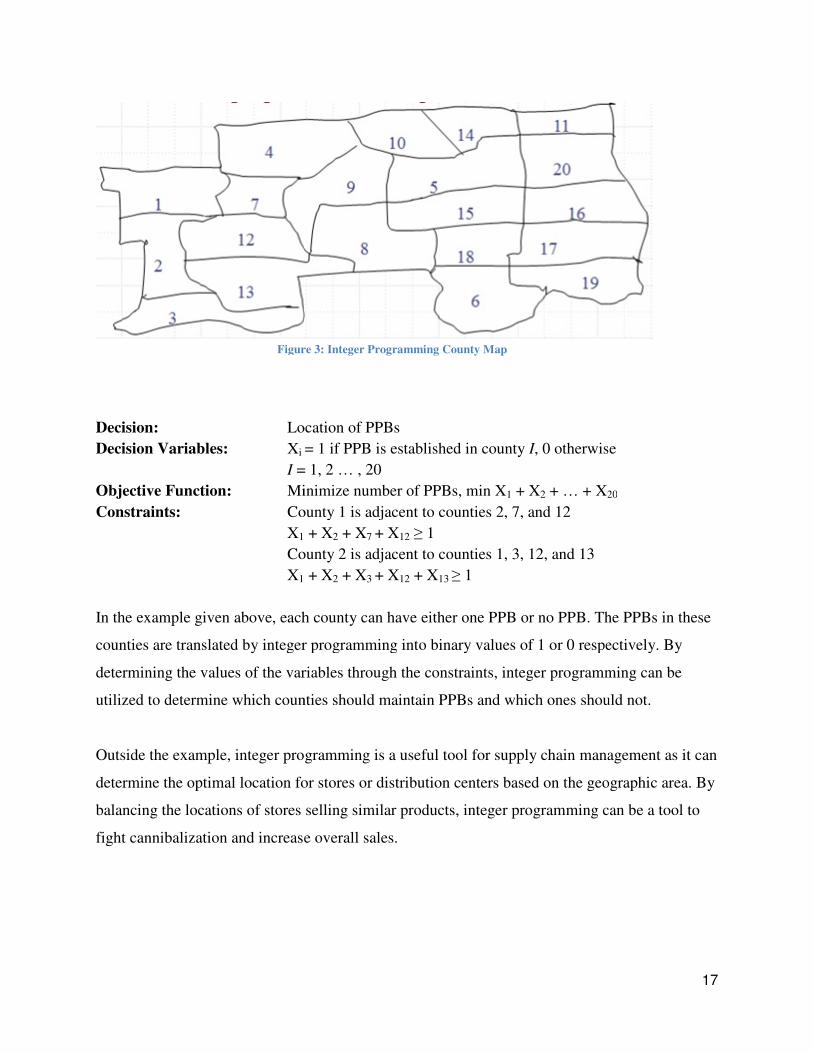
Integer Programming

Integer programming is a type of model where some or all variables are assumed to have integer

values (Freed, 2014). This is useful in facility location (set cover) problems, where the values are

binary (only with 0 or 1 values). In the facility location example, there are 20 counties, shown in

Figure 3 (page 17), which need to be covered by Principle Places of Business (PPBs). The

following is an example of an integer program where binary values are used to determine where

a company will open a facility.

Figure

Decision: Location of PPBs

Decision Variables: Xi

I = 1, 2 … , 20

Objective Function: Minimize number of PPBs, min X

Constraints: County 1 is adjacent to counties 2, 7, and 12

X1

County 2 is adjacent to counties 1, 3, 12, and 13

X1

In the example given above, each county can have either one PPB or no PPB. The PPBs in these

counties are translated by integer programming into binary values of 1 or 0 respectively. By

determining the values of the variables through the constraints, integ

utilized to determine which counties should maintain PPBs and which ones should not.

Outside the example, integer programming is a useful tool for supply chain management as it can

determine the optimal location for stores or distri

balancing the locations of stores selling similar products, integer programming can be a tool to

fight cannibalization and increase overall sales.

Figure 3: Integer Programming County Map

Location of PPBs

i = 1 if PPB is established in county I, 0 otherwise

= 1, 2 … , 20

Minimize number of PPBs, min X1 + X2 + … + X20

County 1 is adjacent to counties 2, 7, and 12

1 + X2 + X7 + X12 ≥ 1

County 2 is adjacent to counties 1, 3, 12, and 13

1 + X2 + X3 + X12 + X13 ≥ 1



determining the values of the variables through the constraints, integer programming can be



determine the optimal location for stores or distribution centers based on the geographic area. By


fight cannibalization and increase overall sales.

17

, 0 otherwise

20



er programming can be



bution centers based on the geographic area. By


18

Design

The following section will discuss the methodology involved in the project. First, the method

used to organize the data will be explained, followed by the long-term and short-term analysis.

Provided Data

Dave Hampton, the Vice President of Go-To Market at Frito Lay, has provided access to sales data in a

given metropolitan area in a Microsoft Excel format. The data provides nearly three years’ worth of sales

values in which each year is divided into 13 4-week periods resulting in a total of 38 sales periods.

Each store is identified by the unique customer number, which refers to the exact store at a specific

longitude and latitude. Description is comprised of the type of store, including but not limited to

convenience stores, supermarkets, mass merchandisers, dollar stores and drug stores. Also incorporated is

level 1 description, which specifies the chain that the store belongs to, and level 2 description, which

specifies the store format. An example of level 1 and 2 store combination would be a Walmart (level 1)

Superstore (level 2). The actual sales numbers are given per 4 week period.

There were a total of 1900 stores with 11 different types, as shown below:

Types of Stores:

Club Line

C-Store (Convenience Store)

Dollar Store

Drug Store

Food Service

Independent Business

Mass Merchandiser

Other Non-UDS (Up-and-Down the Street)

Small Grocery

Supermarket

Vend (Vending Machine) Table 1: List of Store Types Provided

The goal of the project is to determine how much of an effect a store opening or closing has on

neighboring stores based on distance.

19

Organizing Data

The first necessity is to have the ability to sift through the data in order to find stores which could be

geographically related to the store in question.

Because of prior knowledge from the Industrial Engineering curriculum at California Polytechnic State

University, Microsoft Access was the program of choice to filter through the data. Both QBE (Query by

Example) and SQL (Structured Query Language) are used to organize the data.

The stores are then divided into two different types based on the availability of data: complete and

incomplete. A query built using SQL identifies stores from the database which have complete sales data,

or sales values for every period from 2012 to 2014. These stores are known as “complete stores.” All

stores that do not have sales values in every period during the entire interval are labeled as “incomplete

stores.” These incomplete stores include stores which open or close during the given time period, the

primary focus of cannibalization.

Intervention Analysis

The first approach for the problem was to utilize intervention analysis. The sales data for each store

consists of the sales for 38 continuous periods, which reflects a time series. As a type of time series

analysis, intervention analysis combines ARIMA (Autoregressive Integrated Moving Average) modeling

with an intervention to see the effects of an event on a trend. ARIMA has the ability to account for both

seasonal and yearly trends. In intervention analysis, the opening or closing store is the intervention and

the ARIMA model will account for all seasonal and yearly trends.

One of the great challenges in using intervention analysis is learning R, an open-source statistical

software. R has the ability to download packages such as time-series, known as the TSA package, which

can run statistical analysis on the data.

In the end, it was decided not to utilize intervention analysis for two reasons. First, the steep learning

curve of the programming language would have been a great investment of the limited time available for

the project. Second, the problem has extra complexity by incorporating distance as well as time. The TSA

package is able to accommodate time, but distance would involve another type of analysis embedded.

20

Long-term Trends

The objective of long-term analysis is to create a set of charts which track the interaction between a store

which is opening or closing and a neighboring store. On the x-axis is the distance between the store which

is opening or closing and the store being affected. The y-axis displays the deviation from the average

sales experienced by the store being affected. The distance between the two stores can be tracked through

the equation �� , where x1 and y1 are the coordinates of the first store

and x2 and y2 are the coordinates of the second store. This equation takes into account the latitude and

longitude coordinates and the slight asymmetry of the Earth.

On the other hand, the deviation in sales could be found through an X-Bar R chart where the deviations in

sales are shown in the X-Bar chart. By using the MiniTab statistical software, X-bar R charts can be

developed from the data using a subgroup size of 3 because of the need to eliminate excessive deviations

in sales per period. In this scatterplot, the deviation of sales would be a function of the distance between

the two stores. By looking at the chart, an individual could estimate how much the sales of a store would

deviate should a neighboring store open or close. Each interaction between the types of stores is tracked

separately (i.e. an opening mass merchandiser’s effect on a nearby convenience store). A total of three

charts between each interaction are created – 3 periods, 6 periods, and 9 periods after intervention.

One of the greatest challenges to creating future forecasts is to identify trends – both seasonal and yearly.

Seasonal trends are short-term changes which can occur in a matter of a few months. These trends usually

occur every year in a predictable pattern where several months see greater activity than the other months.

In order determine if there is seasonality in the data, visual representations of several random data are

taken in the form of histograms. After visually inspecting the histograms, it can be determined that there

is no truly dominant oscillation in the data (example shown in Figure 4). Because of the lack of a

dominant oscillation, it can be concluded that there is no seasonality which could be accounted for.

21

Figure 4 - Histogram of Mass Merchandisers' Sales in 2012

The year-to-year trend present in the data can be accounted for through the use of a regression analysis

which is performed individually for each store. A regression line for each store is created and the

residuals of the sales can then be tracked and recorded. In order to implement the year-to-year change of

the data, the X-Bar R charts are altered to track the residuals instead of the sales of the original data.

The resulting standard deviations are plotted along with the calculated distances as a scatterplot. In order

to capture an accurate representation of a population, trend lines are then fitted to each scatterplot to find

the overall trend of each interaction between distance and sales deviations. The accuracy of a trend line to

the data that creates it is provided in the form of an R2 value.

Short-term Analysis

Due to the lack of correlation with the long term effects of store closures and openings, the analysis

moves to the investigation of short term effects.

Since analyzing the data in subgroups produced results that were inconclusive, the investigation into

individual measurements was the next step. Individual measurements, as opposed to subgroups, are

common in transactional, business, and service processes for statistical testing. Due to the nature of the

sales data from Frito-Lay, Shewart Control Charts are the most applicable method for analysis.

The use of Individual-Moving Range (I-MR) charts helps to visually determine if any surrounding stores

are impacted by the opening or closing of a particular store. From the I-MR charts, the I chart shows the

$2.60

$2.70

$2.80

$2.90

$3.00

$3.10

$3.20

$3.30

$3.40

$3.50

$3.60

1 2 3 4 5 6 7 8 9 10 11 12 13

Mil

lio

ns

Total Sum of Sales for Mass Merchandisers in

DFW Area (2012)

22

history of the impacted stores sales over the total 38 periods, which is useful in determining if the change

in sales is due to seasonality. The moving range charts indicate the amount of change in sales between the

periods. A good indicator of the introduction or closure of a store having an impact on another

surrounding store is for the sales data point of the neighboring store to go beyond the upper control limit

in the I or MR chart. This is considered a statistically out of control process. For example, in Figure 5, the

store of interest opens during period 2 of 2014 (period 28). As illustrated, the store is beyond the lower

control limit in the period after impact, which means that the change due to impact is probable.

37332925211713951

$100,000.00

$90,000.00

$80,000.00

$70,000.00

$60,000.00

Observation

Individual Value

_X=$80,935.28

UC L=$98,604.14

LC L=$63,266.41

37332925211713951

$20,000.00

$15,000.00

$10,000.00

$5,000.00

$0.00

Observation

Moving Range

__MR=$6,643.49

UC L=$21,706.20

LC L=$0.00

6

51

1

2

2

2

2

I-MR Chart of 11822

Figure 5: I-MR Chart of Impacted Mass Merchandiser Sales from Introduction of Supermarket

After visually inspecting samples of impacted stores’ data, the team thought it would be worth the effort

to track the percentage change in sales from the three periods following the period of impact. The first

period used is the period after the store’s opening or closing because of the need for the first full 4 weeks

of sales.

23

As exhibited by the equations below, sales changes are calculated by computing a percentage difference

of the sales from the period before impact and subtracting that from the first period, second period, and

third period of impact.

�� !�"# %&'"(�)*+,-./� � 0'1�2)*+,-./� � 0'1�2)*+,-.��0'1�2)*+,-.��

�� !�"# %&'"(�)*+,-./ � 0'1�2)*+,-./ � 0'1�2)*+,-.��0'1�2)*+,-.��

�� !�"# %&'"(�)*+,-./3 � 0'1�2)*+,-./3 � 0'1�2)*+,-.��0'1�2)*+,-.��

The purpose of this methodology is to track any trends that could be discovered from plotting the percent

change versus the distance away from the store of interest. However, after plotting the percentage change

against the distance of impact, no visible trends can be seen and there is a lack of correlation between the

two. Therefore, another method is needed due to the inconclusive results.

Needing to prove that the results are statistically significant, the team decided to change the approach on

analysis. To determine the impact made after the first month of the store opening or closing, an analysis is

done using collective averages of each type of store impacted. For instance, if a supermarket opens, the

collective average of the two periods before impact is compared to that of the period of impact and the

next. This is repeated for all opening supermarkets and analyzed for each type of store. Next, the averages

were analyzed through paired t-testing to determine whether the before and after impact averages are

statistically different.

One main issue with this methodology is the limited amount of data supplied to analyze the effect of a

type of store on the varying types of stores. Since the distribution of store locations is not uniform, the

number of stores in the surrounding area is inconsistent. For some impact analyses, there were too few

data points to use a paired t-test. In the “Results” section are the statistically significant percent changes in

sales.

24

Discussion

Included in this section are the results and limitations of the above described analysis. Explanation will

include long-term results, short-term results, followed by some limiting factors.

Long-term Results

The data of the long-term effects were fitted to a logarithmic line. Because the R2 value was anywhere

between 0.08 to 0.15 for the fitted logarithmic line, the data was shown to have no correlation between

distance and sales deviations for periods at least 3 months past the original intervention. The scatterplot

below (Figure 6) shows an example of the deviation of sales of convenience stores within the first three

months after a neighboring supermarket opened. The scatterplot shows that there is little to no correlation

between the distance and the deviation in sales in the long run.

These findings conflicted with the long-term hypothesis that stores sales would be affected by a store

which was either opening or closing nearby. Theoretically, an opening store should negatively impact the

neighboring stores around it. However, as shown in the scatterplot below as Figure 6, there are many

stores which experience a boost in sales within the three months after the opening store intervention. In

the scatterplot, there is one convenience store within one mile of the opening store which experienced a

sales increase of over two standard deviations. One possible explanation for the discrepancy was the sheer

number of neighboring stores which are opening or closing in the 5-mile radius. The large number of

stores which are opening or closing adds extra noise to the dataset which cannot be detected in the model.

Creating a model which can detect other stores which is opening or closing in the neighboring area would

require an extra degree of complexity not present in the current model.

The design of the long-term analysis was a simple and sound model but unfortunately could not factor the

multitude of stores opening or closing in the area. This model most likely would have performed better

had the data been taken from a non-metropolitan area where there are fewer stores.

25

Figure 6: Scatterplot of Distance Versus Deviation in Sales for Mass Merchandisers to Convenience Stores

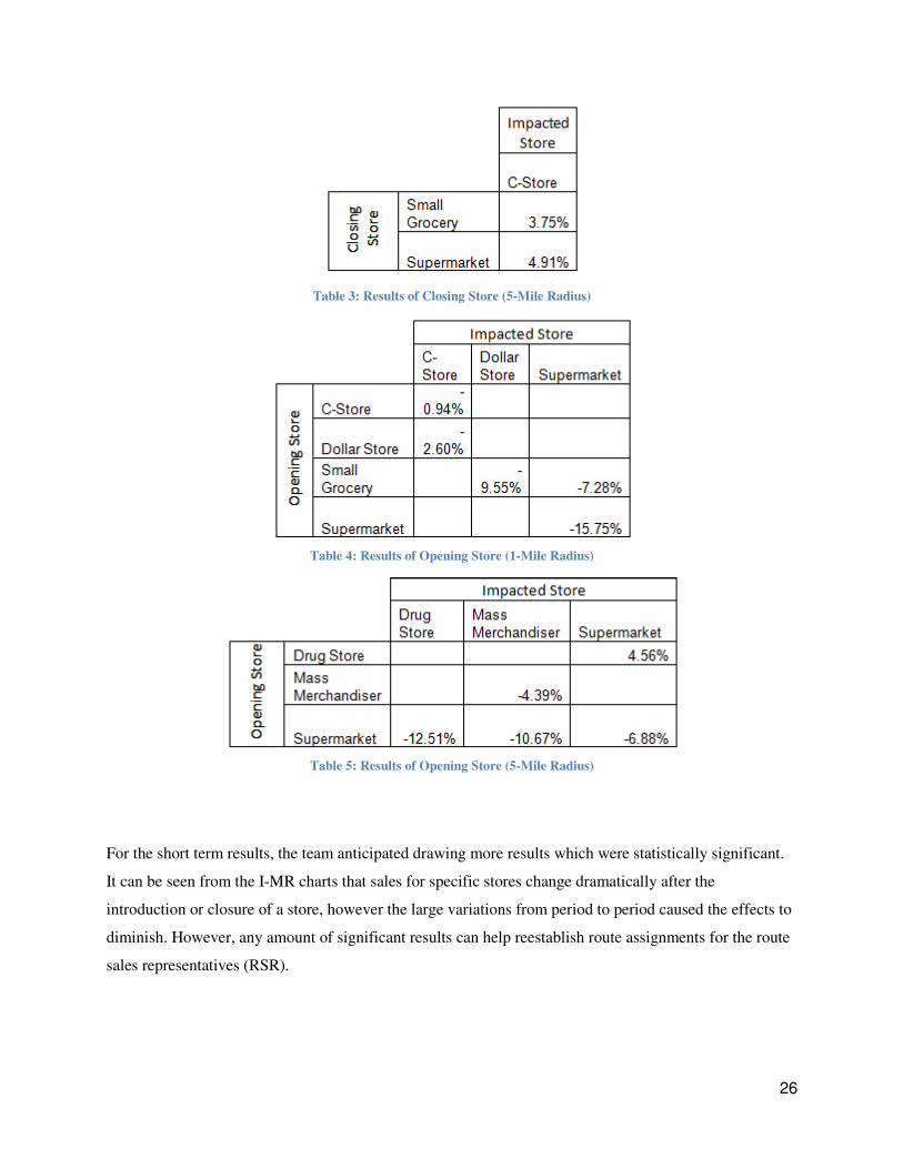
Short-term Results

Results from paired t-testing averages can be seen in Table 2, 3, 4 and 5.The rows denote what type of

store is being closed or opened while the columns denote the type of store that is being evaluated for

changes in sales. Table 2 shows an example of the impact of store closure within a 1-mile radius, while

Table 3 shows the impact of the closure of a store within a 5-mile radius. On the other hand, Table 4

shows the impact of a store introduction with a 1-mile radius and Table 5 shows the impact of a store

introduction within a 5-mile radius.

Table 2: Results of Closing Store (1-Mile Radius)

-4

-3

-2

-1

0

1

2

3

0 1 2 3 4 5 6 7 8

First Three Months After Opening Store Intervention

26

Table 3: Results of Closing Store (5-Mile Radius)

Table 4: Results of Opening Store (1-Mile Radius)

Table 5: Results of Opening Store (5-Mile Radius)

For the short term results, the team anticipated drawing more results which were statistically significant.

It can be seen from the I-MR charts that sales for specific stores change dramatically after the

introduction or closure of a store, however the large variations from period to period caused the effects to

diminish. However, any amount of significant results can help reestablish route assignments for the route

sales representatives (RSR).

27

Limitations

As mentioned previously, there are many factors that affect the sales of particular stores in an area, and

each factor cannot always be accounted for. For example, sales of a store closer to a highway would

typically be higher than the sales of an otherwise equivalent store further away from a highway. The

contributing factor would be proximity to a major thoroughfare, which was not a factor evaluated in this

analysis due to the absence of this data. Though the analysis of seasonality and year-to-year trends was

completed, the countless other factors were not analyzed.

The inability to quantify many of these factors calls into question the sales values that were utilized in the

above analysis. Since most of the average differences came back with large p-values in the paired t-test,

this proposes that there is no effect on surrounding stores when a store opens or closes which does not

appear to align with what theory would suggest. Therefore, it is probable that the countless factors which

were unable to be analyzed affected the sales significantly.

Further analysis into said factors is necessary. This can be investigated through a more detailed regression

analysis, intervention analysis, or one of many other methods. It remains to be determined how to most

accurately compare different markets with different chains which are dynamic through time.

28

Conclusions

While the long-term effects cannot support any statistically significant conclusions, the short-

term effects show a promising lead. The paired t-test validates the hypothesis that an intervening

mass merchandiser or supermarket can affect the sales of their neighboring respective stores but

does not have an effect other types of stores. This means that a customer who shops at a mass

merchandiser will continue to shop at a different mass merchandiser, instead of a dollar store or

supermarket, should the original store close. Frito-Lay has the current practice of assuming that

approximately 90% of sales are cannibalized. The short-term findings provide support for this

theory.

The analysis completed on sales data for Frito-Lay does not solely apply to Frito-Lay — the

importance of this type of analysis spreads much farther. One such application lies in the

recommendation to store chains that a best plan of action when opening a store is to do so

outside of a 5-mile radius. For example, if a Kroger opens within a short distance of another

Kroger, it is highly possible that the new store’s sales will simply be cannibalized from the

existing store, rather than inducing an increment in overall sales. In short, while only sales

numbers for Frito-Lay have been examined, it is possible to expand the results to other

industries.

29

Works Cited

1. Freed, Tali. “Integer Programming.” PDF, 2014. Nov. 18 2014.

2. Hormazi, Amir M., and Stacy Giles. "Data Mining: A Competitive Weapon For Banking

and Retail Industries." Information Systems Management 21.2 (2004): 62-71. ProQuest.

5 Nov. 2014.

3. Lomax, Wendy, Kathy Hammond, Robert East, and Maria Clemente. “The Measurement

of Cannibalization.” The Journal of Product and Brand Management 6.1 (1997): 27-39.

ProQuest. 5 Nov 2014.

4. Ming-Long, Lee, and R. Kelley Pace. "Spatial Distribution of Retail Sales." Journal of

Real Estate Finance and Economics 31.1 (2005): 53-69. ProQuest. 6 Nov. 2014.

5. Nachiappan, SP, N. Jawahar, S. Parthibaraj, and B. Brucelee. “Performance Analysis of

Forecast Driven Vendor Managed Inventory System.” Journal of Advanced

Manufacturing Systems 4.2 (2005): 209-226. ProQuest. 10 Nov 2014.

6. Pancras, Joseph, S. Sriram, and V Kumar. “Empirical Investigation of Retail Expansion

and Cannibalization in a Dynamic Environment.” Management Science 58(11) (2012):

2001-2018. Engineering Village. 7 Nov 2014.

7. Rupnik, Rok, Matjaz Kukar, and Marjan Krisper. "Integrating Data Mining and Decision

Support Through Data Mining Based Decision Support System." The Journal of

Computer Information Systems 47.3 (2007): 89-104. ProQuest. 5 Nov. 2014.

8. Zoltners, Andris A., and Prabhakant Sinha. "The 2004 ISMS Practice Prize Winner: Sales

Territory Design: Thirty Years of Modelng and Implementation." Marketing Science 24.3

(2005): 313-31. ProQuest. 2 Nov. 2014.

30

Appendix

Test Results for I Chart of 11822

TEST 1. One point more than 3.00 standard deviations from center line.

Test Failed at points: 29, 30

TEST 2. 9 points in a row on same side of center line.

Test Failed at points: 21, 22, 23

TEST 5. 2 out of 3 points more than 2 standard deviations from center line (on

one side of CL).

Test Failed at points: 30, 37

TEST 6. 4 out of 5 points more than 1 standard deviation from center line (on

one side of CL).

Test Failed at points: 38

Test Results for MR Chart of 11822

TEST 2. 9 points in a row on same side of center line.

Test Failed at points: 25

* WARNING * If graph is updated with new data, the results above may no

* longer be correct.

Documents

Frito-Lay - Supply Chain Impact Analysis