PHYSICAL REVIEW B 93, 205117 (2016)

Friedel oscillations as a probe of fermionic quasiparticles

Emanuele G. Dalla Torre,1,2 David Benjamin,2 Yang He,2 David Dentelski,1 and Eugene Demler2

1Department of Physics, Bar Ilan University, Ramat Gan 5290002, Israel2Department of Physics, Harvard University, Cambridge, Massachusetts 02138, USA

(Received 21 July 2015; published 11 May 2016)

When immersed in a sea of electrons, local impurities give rise to density modulations known as Friedeloscillations. In spite of the generality of this phenomenon, the exact shape of these modulations is usuallycomputed only for noninteracting electrons with a quadratic dispersion relation. In actual materials, Friedeloscillations are a viable way to access the properties of electronic quasiparticles, including their dispersionrelation, lifetime, and pairing. In this work we analyze the signatures of Friedel oscillations in STM and x-rayscattering experiments, focusing on the concrete example of cuprate superconductors. We identify signaturesof Friedel oscillations seeded by impurities and vortices, and explain experimental observations that have beenpreviously attributed to a competing charge order.

DOI: 10.1103/PhysRevB.93.205117

I. INTRODUCTION

In the study of strongly correlated materials, one ofthe common themes is the appearance of competing and/orintertwined orders (see for example Refs. [1–3] for a review).Recently this subject received considerable attention due to theexperimental observation of incommensurate charge modula-tions that coexist with high-temperature superconductivity incuprates [4–12]. These modulations were originally observedon the surface of BSCCO via scanning tunneling spectroscopy(STM) [13–16], and recently found in the bulk of YBCO andother materials by x-ray scattering experiments [4–9]. It iscommonly believed that these modulations are adiabaticallyconnected to the long-ranged charge order observed at largemagnetic fields by quantum oscillations [17,18] and nuclearmagnetic resonance (NMR) [19]. In our earlier work [20]we proposed an alternative interpretation: the modulationsobserved at small magnetic fields can be understood as Friedeloscillations due to the scattering of quasiparticles with a shortlifetime, rather than as the evidence of a competing order.

Friedel oscillations are density modulations generated bylocal impurities acting on mobile charges, such as electronsin a metal. At the lowest order of perturbation theory, thesemodulations are proportional to the static density-densityresponse function of the unperturbed (homogeneous) system.For free electrons in three dimensions, this function can beanalytically computed and its Fourier transform is peaked attwice the Fermi wave vector (see Ref. [21] for a review).As a consequence, Friedel oscillations can be exploited todirectly measure the electron density [22,23]. In more complexmaterials the shape of Friedel oscillations is determined by theband structure of fermionic quasiparticles, their lifetime, andthe presence of a pairing gap. We suggest that the observationof Friedel oscillations is therefore a viable tool for studying theproperties of quasiparticles in strongly correlated materials.

In this paper we theoretically analyze signatures of Friedeloscillations in x-ray and STM experiments, focusing onthe specific example of superconducting cuprates. The bandstructures of these materials have been extensively studied byangle-resolved photoemission spectroscopy (ARPES). In thenormal phase, these materials have a single Fermi surface,whose phenomenological parameters are well known. This

information allows us to make quantitative predictions for theexpected shape of the Freidel oscillations. At low tempera-tures, the presence of a superconducting gap challenges themain assumption of Friedel oscillations, namely the presenceof an underlying Fermi liquid. As we will see below, Friedeloscillations can occur in a paired state as well, with someimportant differences. In particular, in a superconductor,Friedel oscillations can be seeded by both local modulationsof the chemical potential (as in normal metal) and localmodulations of the pairing gap.

In the following we first present the theoretical frameworkused to analyze Friedel oscillations (Sec. II) and then discussits implications for recent experiments in cuprates (Sec. III).The Appendixes explain in detail several technical details ofthe calculations and in particular how to perform an ensembleaverage over static impurities (Appendix A 1); how to derivethe formalism of resonant elastic scattering using Green’sfunctions (Appendix A 2) and how to relate it to the Lindhardsusceptibility (Appendix A 3); and how to quantify the effectsof the spin-orbit coupling (Appendix A 4) and of the light-fieldpolarization (Appendix A 5).

II. THEORETICAL FRAMEWORK

A. Lindhard susceptibility

We open our theoretical description of Friedel oscillationsby considering (hard) x-ray scattering experiments. This probewas used to detect Friedel oscillations in vanadium-dopedblue bronze [24], a charge density wave (CDW) material. Forthis material, accurate x-ray scattering experiments revealedtwo distinct incommensurate diffraction peaks. These peakswere respectively identified with the CDW wave vector, andwith Friedel oscillations at twice the Fermi wave vector. In anonresonant x-ray experiment the intensity of the scatteredlight is proportional to the zero-frequency density-densityresponse function [25]

χ (q) =∫ ∞

0dt

∫dxeiq·x〈[ρ(x,t),ρ(x,0)]〉, (1)

where [·,·] is the commutation relation and ρ(x,t) =ψ†(x,t)ψ(x,t) is the charge density. For quasiparticles with a

2469-9950/2016/93(20)/205117(15) 205117-1 ©2016 American Physical Society

DALLA TORRE, BENJAMIN, HE, DENTELSKI, AND DEMLER PHYSICAL REVIEW B 93, 205117 (2016)

dispersion relation εk and a finite lifetime �, Eq. (1) becomes

χ (q) =∑

k

nk − nk+q

εk − εk+q + 2i�, (2)

where nk = {1 + exp[(εk − μ)/T ]}−1 is the Fermi-Dirac dis-tribution function, and T is the temperature. By neglectinginteractions between quasiparticles, Eq. (2) disregards possiblecollective modes such as spin waves and paramagnons. Inthe case of free electrons (with εk = k2/2m and � → 0+)and at T = 0, Eq. (2) can be evaluated analytically [21]. Intwo dimensions χ (q) is momentum independent for q < 2kF ,and decays algebraically for q > 2kF , where kF is the Fermimomentum [26]. In actual materials, the dispersion relation ismore complex and an exact analytical evaluation of Eq. (2)is generically not possible. We therefore resort to a numericalevaluation of this expression. As we will see in Sec. III A, thiscalculation leads to sharp peaks in χ (q). When such peaks areobserved in experiments, they may be interpreted as evidenceof static charge density waves (CDW).

B. Local density of states

In contrast to hard x-ray measurements, STM and REXStemporarily change the number of electrons in the conductionband and couple to the density of states, rather than to thedensity-density response function [27]. Specifically, at zerotemperature the STM differential conductivity dI (r)/dV isproportional to the local density of states g(r,ω = V ), givenby the imaginary part of the retarded Green’s function:

g(r,ω) = Im[G(r,ω)] (3)

= Im

[∫ ∞

0dte−iω(t−t ′)〈[ψ†(r,t),ψ(r,t ′)]〉

]. (4)

For disordered materials, g(r,ω) varies in space and is ingeneral unpredictable. It is therefore common to compute thetwo-dimensional Fourier transform of the signal at a fixedvoltage [23]

g(q,ω) =∫

ddreiq·rg(r,ω). (5)

As we will explain in detail below, the absolute value of g(q,ω)depends on the types of scatterers present in the material, butnot on their position (assuming that the sample is large enoughto enable self-averaging of the scatterers’ position).

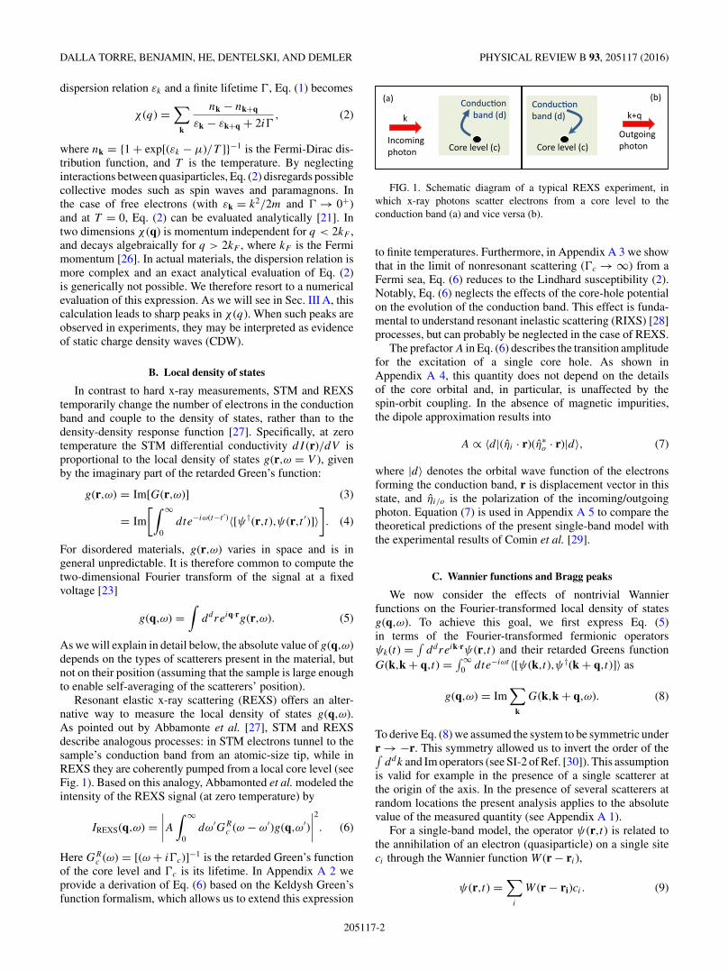
Resonant elastic x-ray scattering (REXS) offers an alter-native way to measure the local density of states g(q,ω).As pointed out by Abbamonte et al. [27], STM and REXSdescribe analogous processes: in STM electrons tunnel to thesample’s conduction band from an atomic-size tip, while inREXS they are coherently pumped from a local core level (seeFig. 1). Based on this analogy, Abbamonted et al. modeled theintensity of the REXS signal (at zero temperature) by

IREXS(q,ω) =∣∣∣∣A

∫ ∞

0dω′GR

c (ω − ω′)g(q,ω′)∣∣∣∣2

. (6)

Here GRc (ω) = [(ω + i�c)]−1 is the retarded Green’s function

of the core level and �c is its lifetime. In Appendix A 2 weprovide a derivation of Eq. (6) based on the Keldysh Green’sfunction formalism, which allows us to extend this expression

Conduc�on band (d)

Core level (c)

Conduc�on band (d)

Core level (c)

k

Incoming photon

k+q

Outgoing photon

(a) (b)

FIG. 1. Schematic diagram of a typical REXS experiment, inwhich x-ray photons scatter electrons from a core level to theconduction band (a) and vice versa (b).

to finite temperatures. Furthermore, in Appendix A 3 we showthat in the limit of nonresonant scattering (�c → ∞) from aFermi sea, Eq. (6) reduces to the Lindhard susceptibility (2).Notably, Eq. (6) neglects the effects of the core-hole potentialon the evolution of the conduction band. This effect is funda-mental to understand resonant inelastic scattering (RIXS) [28]processes, but can probably be neglected in the case of REXS.

The prefactor A in Eq. (6) describes the transition amplitudefor the excitation of a single core hole. As shown inAppendix A 4, this quantity does not depend on the detailsof the core orbital and, in particular, is unaffected by thespin-orbit coupling. In the absence of magnetic impurities,the dipole approximation results into

A ∝ 〈d|(ηi · r)(η∗o · r)|d〉, (7)

where |d〉 denotes the orbital wave function of the electronsforming the conduction band, r is displacement vector in thisstate, and ηi/o is the polarization of the incoming/outgoingphoton. Equation (7) is used in Appendix A 5 to compare thetheoretical predictions of the present single-band model withthe experimental results of Comin et al. [29].

C. Wannier functions and Bragg peaks

We now consider the effects of nontrivial Wannierfunctions on the Fourier-transformed local density of statesg(q,ω). To achieve this goal, we first express Eq. (5)in terms of the Fourier-transformed fermionic operatorsψk(t) = ∫

ddreik·rψ(r,t) and their retarded Greens functionG(k,k + q,t) = ∫ ∞

0 dte−iωt 〈[ψ(k,t),ψ†(k + q,t)]〉 as

g(q,ω) = Im∑

k

G(k,k + q,ω). (8)

To derive Eq. (8) we assumed the system to be symmetric underr → −r. This symmetry allowed us to invert the order of the∫

ddk and Im operators (see SI-2 of Ref. [30]). This assumptionis valid for example in the presence of a single scatterer atthe origin of the axis. In the presence of several scatterers atrandom locations the present analysis applies to the absolutevalue of the measured quantity (see Appendix A 1).

For a single-band model, the operator ψ(r,t) is related tothe annihilation of an electron (quasiparticle) on a single siteci through the Wannier function W (r − ri),

ψ(r,t) =∑

i

W (r − ri)ci . (9)

205117-2

FRIEDEL OSCILLATIONS AS A PROBE OF FERMIONIC . . . PHYSICAL REVIEW B 93, 205117 (2016)

Combining Eqs. (8) and (9) we arrive at the expression [30–33]

g(q,ω) = Im∑

k

W ∗k Glattice(k,k + q,ω)Wk+q, (10)

where W (k) = ∫ddreik·rW (r), Glattice(k,k+q,ω) =∫ ∞

0 dte−iωt

〈[c(k,t),c†(k + q,t)]〉, and ck = ∑i e

ik·xi ci . Note that bydefinition, Glattice(k,k + q,ω) is a periodic function of kand q with a period given by the Bravais lattice vec-tors G. In the absence of impurities Glattice(k,k + q,ω) =G(k,ω)

∑G δ(q − G), where G(k,ω) = G(k,k,ω). This ex-

pression gives rise to well-defined Bragg peaks in g(q,ω),whose intensity is determined by the width of the Wannierfunction.

Cuprates posses a nontrivial Wannier function with d-wavesymmetry [34]. As explained in Ref. [35], this shape affects thephase and intensity of the Fourier-transformed STM signal at alarge wave vector (beyond the central Brillouin zone), leadingto subtle correlations that were interpreted as evidence of acompeting order with d-form factor [10–12]. In this paper wefocus on the central Brillouin zone, where the precise shape ofthe Wannier function is not very important. For convenience,we then approximate W (k) as a Gaussian wave function withwidth σk = 1.8(2π/a), where a is the lattice constant.

D. Scattering from local impurities

In actual materials, as a consequence of disorder, theFourier-transformed density of states g(q,ω) is nonzero evenfor wave vectors that do not correspond to a lattice vector.Performing a first-order perturbation theory in the scatteringpotential (Born approximation) one finds [36]

G(k,k + q,ω) = G(k,ω)∑

G

δ(q − G)

+ G(k,ω)T (k,q)G(k + q,ω), (11)

where G(k,ω) = G(k,k,ω), and T (k,q) describes the scatter-ing of quasiparticles from momentum k to momentum k + q.

One of the main goals of this paper is to consider theeffects of different types of impurities, defined through theirscattering matrices T . We consider here only perturbationsthat are static and quadratic in the quasiparticles’ creation andannihilation operators. Any such perturbation can be describedby the Hamiltonian

Hpert = Vi,j c†i cj =

∑k,q

T (k,q)c†kck+q, (12)

where T (k,q) = ∑i,j Vi,j (eiq·xj eik·(xi−xj ) + eiq·xi eik·(xj −xi )).

If the scatterer acts on a single site (or on the bonds linkedto a single site), the scattering amplitude is given by the sumof two terms, which depend respectively on the momentumof the incoming and outgoing quasiparticles only: T (k,q) =Tk + Tk+q. Combining this expression with Eq. (8) we find

g(q,ω) =∑

k

Im[W ∗

k G(k,ω)Wk+q]∑

G

δ(q − G)

+∑

k

Im[W ∗k G(k,ω)(Tk+Tk+q)G(k + q,ω)Wk+q].

(13)

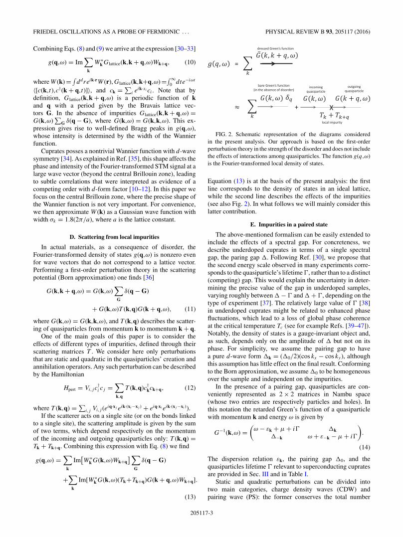
FIG. 2. Schematic representation of the diagrams consideredin the present analysis. Our approach is based on the first-orderperturbation theory in the strength of the disorder and does not includethe effects of interactions among quasiparticles. The function g(q,ω)is the Fourier-transformed local density of states.

Equation (13) is at the basis of the present analysis: the firstline corresponds to the density of states in an ideal lattice,while the second line describes the effects of the impurities(see also Fig. 2). In what follows we will mainly consider thislatter contribution.

E. Impurities in a paired state

The above-mentioned formalism can be easily extended toinclude the effects of a spectral gap. For concreteness, wedescribe underdoped cuprates in terms of a single spectralgap, the paring gap �. Following Ref. [30], we propose thatthe second energy scale observed in many experiments corre-sponds to the quasiparticle’s lifetime �, rather than to a distinct(competing) gap. This would explain the uncertainty in deter-mining the precise value of the gap in underdoped samples,varying roughly between � − � and � + �, depending on thetype of experiment [37]. The relatively large value of � [38]in underdoped cuprates might be related to enhanced phasefluctuations, which lead to a loss of global phase coherenceat the critical temperature Tc (see for example Refs. [39–47]).Notably, the density of states is a gauge-invariant object and,as such, depends only on the amplitude of � but not on itsphase. For simplicity, we assume the pairing gap to havea pure d-wave form �k = (�0/2)(cos kx − cos ky), althoughthis assumption has little effect on the final result. Conformingto the Born approximation, we assume �0 to be homogeneousover the sample and independent on the impurities.

In the presence of a pairing gap, quasiparticles are con-veniently represented as 2 × 2 matrices in Nambu space(whose two entries are respectively particles and holes). Inthis notation the retarded Green’s function of a quasiparticlewith momentum k and energy ω is given by

G−1(k,ω) =(

ω − εk + μ + i� �k�−k ω + ε−k − μ + i�

).

(14)

The dispersion relation εk, the pairing gap �0, and thequasiparticles lifetime � relevant to superconducting cupratesare provided in Sec. III and in Table I.

Static and quadratic perturbations can be divided intotwo main categories, charge density waves (CDW) andpairing wave (PS): the former conserves the total number

205117-3

DALLA TORRE, BENJAMIN, HE, DENTELSKI, AND DEMLER PHYSICAL REVIEW B 93, 205117 (2016)

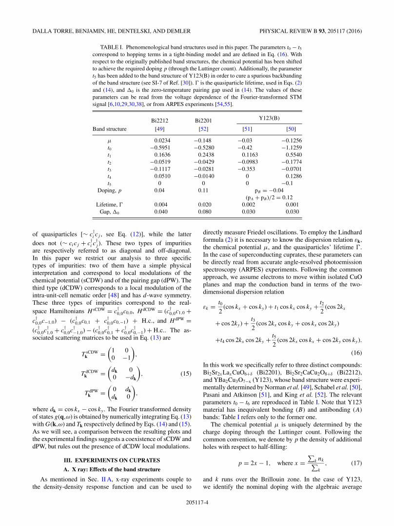
TABLE I. Phenomenological band structures used in this paper. The parameters t0 − t5correspond to hopping terms in a tight-binding model and are defined in Eq. (16). Withrespect to the originally published band structures, the chemical potential has been shiftedto achieve the required doping p (through the Luttinger count). Additionally, the parametert5 has been added to the band structure of Y123(B) in order to cure a spurious backbandingof the band structure (see SI-7 of Ref. [30]). � is the quasiparticle lifetime, used in Eqs. (2)and (14), and �0 is the zero-temperature pairing gap used in (14). The values of theseparameters can be read from the voltage dependence of the Fourier-transformed STMsignal [6,10,29,30,38], or from ARPES experiments [54,55].

Bi2212 Bi2201 Y123(B)

Band structure [49] [52] [51] [50]

μ 0.0234 −0.148 −0.03 −0.1256t0 −0.5951 −0.5280 −0.42 −1.1259t1 0.1636 0.2438 0.1163 0.5540t2 −0.0519 −0.0429 −0.0983 −0.1774t3 −0.1117 −0.0281 −0.353 −0.0701t4 0.0510 −0.0140 0 0.1286t5 0 0 0 −0.1

Doping, p 0.04 0.11 pB = −0.04(pA + pB )/2 = 0.12

Lifetime, � 0.004 0.020 0.002 0.001Gap, �0 0.040 0.080 0.030 0.030

of quasiparticles [∼ c†i cj , see Eq. (12)], while the latter

does not (∼ cicj + c†i c

†j ). These two types of impurities

are respectively referred to as diagonal and off-diagonal.In this paper we restrict our analysis to three specifictypes of impurities: two of them have a simple physicalinterpretation and correspond to local modulations of thechemical potential (sCDW) and of the pairing gap (dPW). Thethird type (dCDW) corresponds to a local modulation of theintra-unit-cell nematic order [48] and has d-wave symmetry.These three types of impurities correspond to the real-space Hamiltonians H sCDW = c

†0,0c0,0, H dCDW = (c†0,0c1,0 +

c†0,0c−1,0) − (c†0,0c0,1 + c

†0,0c0,−1) + H.c., and H dPW =

(c†0,0c†1,0 + c

†0,0c

†−1,0) − (c†0,0c

†0,1 + c

†0,0c

†0,−1) + H.c.. The as-

sociated scattering matrices to be used in Eq. (13) are

T sCDWk =

(1 00 −1

),

T dCDWk =

(dk 00 −dk

), (15)

T dPWk =

(0 dkdk 0

),

where dk = cos kx − cos ky . The Fourier transformed densityof states g(q,ω) is obtained by numerically integrating Eq. (13)with G(k,ω) and Tk respectively defined by Eqs. (14) and (15).As we will see, a comparison between the resulting plots andthe experimental findings suggests a coexistence of sCDW anddPW, but rules out the presence of dCDW local modulations.

III. EXPERIMENTS ON CUPRATES

A. X ray: Effects of the band structure

As mentioned in Sec. II A, x-ray experiments couple tothe density-density response function and can be used to

directly measure Friedel oscillations. To employ the Lindhardformula (2) it is necessary to know the dispersion relation εk,the chemical potential μ, and the quasiparticles’ lifetime �.In the case of superconducting cuprates, these parameters canbe directly read from accurate angle-resolved photoemissionspectroscopy (ARPES) experiments. Following the commonapproach, we assume electrons to move within isolated CuOplanes and map the conduction band in terms of the two-dimensional dispersion relation

εk = t0

2(cos kx + cos ky) + t1 cos kx cos ky + t2

2(cos 2kx

+ cos 2ky) + t3

2(cos 2kx cos ky + cos kx cos 2ky)

+t4 cos 2kx cos 2ky + t5

2(cos 2kx cos kx + cos 2ky cos ky).

(16)

In this work we specifically refer to three distinct compounds:Bi2Sr2xLaxCuO6+δ (Bi2201), Bi2Sr2CaCu2O8+δ (Bi2212),and YBa2Cu3O7−x (Y123), whose band structure were experi-mentally determined by Norman et al. [49], Schabel et al. [50],Pasani and Atkinson [51], and King et al. [52]. The relevantparameters t0 − t6 are reproduced in Table I. Note that Y123material has inequivalent bonding (B) and antibonding (A)bands: Table I refers only to the former one.

The chemical potential μ is uniquely determined by thecharge doping through the Luttinger count. Following thecommon convention, we denote by p the density of additionalholes with respect to half-filling:

p = 2x − 1, where x =∑

k nk∑k

, (17)

and k runs over the Brillouin zone. In the case of Y123,we identify the nominal doping with the algebraic average

205117-4

FRIEDEL OSCILLATIONS AS A PROBE OF FERMIONIC . . . PHYSICAL REVIEW B 93, 205117 (2016)

−1 −0.5 0 0.5 1−1

−0.5

0

0.5

1(a)

kx/π

k y/π 0.2 0.3 0.40

0.5

1

0 0.1 0.2 0.3 0.4 0.50

0.2

0.4

0.6

0.8

1

χ(q)

qx/(2π)

(b)

0.2 0.30.6

0.8

1

0.2 0.30.2

0.3

0.4

0.5

Bi2212La2201Y123(B) [50]Y123(B) [49]

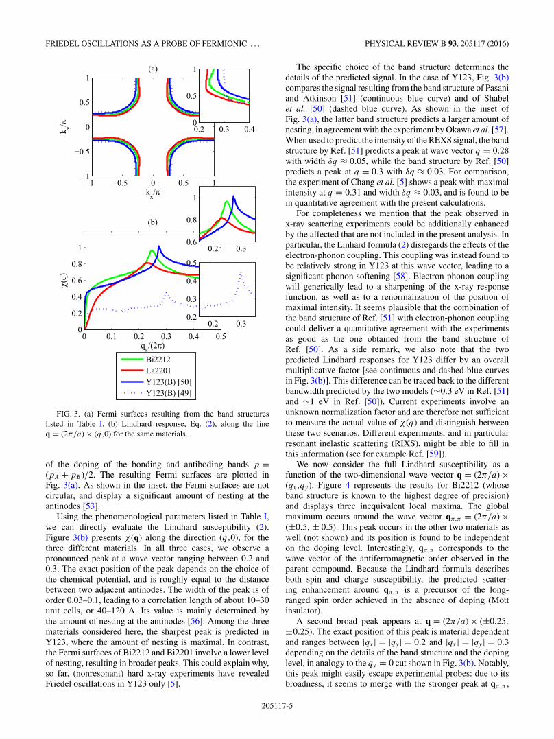
FIG. 3. (a) Fermi surfaces resulting from the band structureslisted in Table I. (b) Lindhard response, Eq. (2), along the lineq = (2π/a) × (q,0) for the same materials.

of the doping of the bonding and antiboding bands p =(pA + pB)/2. The resulting Fermi surfaces are plotted inFig. 3(a). As shown in the inset, the Fermi surfaces are notcircular, and display a significant amount of nesting at theantinodes [53].

Using the phenomenological parameters listed in Table I,we can directly evaluate the Lindhard susceptibility (2).Figure 3(b) presents χ (q) along the direction (q,0), for thethree different materials. In all three cases, we observe apronounced peak at a wave vector ranging between 0.2 and0.3. The exact position of the peak depends on the choice ofthe chemical potential, and is roughly equal to the distancebetween two adjacent antinodes. The width of the peak is oforder 0.03–0.1, leading to a correlation length of about 10–30unit cells, or 40–120 A. Its value is mainly determined bythe amount of nesting at the antinodes [56]: Among the threematerials considered here, the sharpest peak is predicted inY123, where the amount of nesting is maximal. In contrast,the Fermi surfaces of Bi2212 and Bi2201 involve a lower levelof nesting, resulting in broader peaks. This could explain why,so far, (nonresonant) hard x-ray experiments have revealedFriedel oscillations in Y123 only [5].

The specific choice of the band structure determines thedetails of the predicted signal. In the case of Y123, Fig. 3(b)compares the signal resulting from the band structure of Pasaniand Atkinson [51] (continuous blue curve) and of Shabelet al. [50] (dashed blue curve). As shown in the inset ofFig. 3(a), the latter band structure predicts a larger amount ofnesting, in agreement with the experiment by Okawa et al. [57].When used to predict the intensity of the REXS signal, the bandstructure by Ref. [51] predicts a peak at wave vector q = 0.28with width δq ≈ 0.05, while the band structure by Ref. [50]predicts a peak at q = 0.3 with δq ≈ 0.03. For comparison,the experiment of Chang et al. [5] shows a peak with maximalintensity at q = 0.31 and width δq ≈ 0.03, and is found to bein quantitative agreement with the present calculations.

For completeness we mention that the peak observed inx-ray scattering experiments could be additionally enhancedby the affected that are not included in the present analysis. Inparticular, the Linhard formula (2) disregards the effects of theelectron-phonon coupling. This coupling was instead found tobe relatively strong in Y123 at this wave vector, leading to asignificant phonon softening [58]. Electron-phonon couplingwill generically lead to a sharpening of the x-ray responsefunction, as well as to a renormalization of the position ofmaximal intensity. It seems plausible that the combination ofthe band structure of Ref. [51] with electron-phonon couplingcould deliver a quantitative agreement with the experimentsas good as the one obtained from the band structure ofRef. [50]. As a side remark, we also note that the twopredicted Lindhard responses for Y123 differ by an overallmultiplicative factor [see continuous and dashed blue curvesin Fig. 3(b)]. This difference can be traced back to the differentbandwidth predicted by the two models (∼0.3 eV in Ref. [51]and ∼1 eV in Ref. [50]). Current experiments involve anunknown normalization factor and are therefore not sufficientto measure the actual value of χ (q) and distinguish betweenthese two scenarios. Different experiments, and in particularresonant inelastic scattering (RIXS), might be able to fill inthis information (see for example Ref. [59]).

We now consider the full Lindhard susceptibility as afunction of the two-dimensional wave vector q = (2π/a) ×(qx,qy). Figure 4 represents the results for Bi2212 (whoseband structure is known to the highest degree of precision)and displays three inequivalent local maxima. The globalmaximum occurs around the wave vector qπ,π = (2π/a) ×(±0.5, ± 0.5). This peak occurs in the other two materials aswell (not shown) and its position is found to be independenton the doping level. Interestingly, qπ,π corresponds to thewave vector of the antiferromagnetic order observed in theparent compound. Because the Lindhard formula describesboth spin and charge susceptibility, the predicted scatter-ing enhancement around qπ,π is a precursor of the long-ranged spin order achieved in the absence of doping (Mottinsulator).

A second broad peak appears at q = (2π/a) × (±0.25,

±0.25). The exact position of this peak is material dependentand ranges between |qx | = |qy | = 0.2 and |qx | = |qy | = 0.3depending on the details of the band structure and the dopinglevel, in analogy to the qy = 0 cut shown in Fig. 3(b). Notably,this peak might easily escape experimental probes: due to itsbroadness, it seems to merge with the stronger peak at qπ,π ,

205117-5

DALLA TORRE, BENJAMIN, HE, DENTELSKI, AND DEMLER PHYSICAL REVIEW B 93, 205117 (2016)

FIG. 4. Lindhard response Eq. (2) as a function of q = (2π/a) ×(qx,qy) for Bi2212. The response of the other materials is qualitativelysimilar (although the peak position is shifted away from q = 0.25).

especially if only the cut along the line qx = qy is available. Wewill come back to this point in Sec. III C. Finally, the third localmaximum occurs at q = (±0.25, ± 0.1): the wave vector q =(2π/a) × (±0.25,0) is predicted to be a saddle point sittingbetween these local maxima. We note that a similar behaviorwas observed in recent experiments by Thampy et al. [60], whofound sharp peaks at q = (2π/a) × (0.25, ± 0.015), separatedby a saddle point at q = (2π/a) × (0.25,0) [61].

B. STM: Dispersive vs nondispersive peaks

We now proceed to discuss STM experiments, by firstoffering a brief summary of the main results of Ref. [30].Specifically, in that paper we related the emergence ofnondispersive peaks in underdoped cuprates to their relativelylarge inverse quasiparticle lifetime �. In materials where �

is small (such as overdoped cuprates), the STM probe excitesquasiparticles with an energy that precisely corresponds tothe tip-sample voltage. In this case, energy and momentumconservation leads to the well-known “octet model” [62]. Thismodel predicts the emergence of seven inequivalent dispersivepeaks, which can be found by connecting points on the Fermisurface where the pairing gap is equivalent to the tip-samplevoltage. As shown for example by Nowadnick et al. [36], thesepeaks are indeed reproduced by Eq. (13) in the limit of � → 0.In contrast, for a finite �, the argument leading to the octetmodel does not apply because the quasiparticles’ energy is notconserved. In this case, a numerical evaluation of Eq. (13) isnecessary. As shown in Ref. [30] these calculations lead tonondispersive peaks around the wave vectors connecting theantinodes. These scattering wave vectors are enhanced at allvoltages for two reasons: (i) Any scattering is enhanced at theantinodes due to the Fermi surface nesting (in analogy to theanalysis of Sec. III A); and (ii) the modulations of the pairinggap T dPW

k in Eq. (15) are proportional to the pairing gap �kand are therefore enhanced at the antinodes, where the latteris maximal.

The effect of � on the calculated STM maps is highlightedin Fig. 5, where � varies from 1 meV [Fig. 5(a)] to 20 meV

(a) Γ=1meV

qx

0 0.25 0.5

V [m

eV]

0

10

20

30

40(b) Γ=20meV

qx

0 0.25 0.50

10

20

30

40

min

max

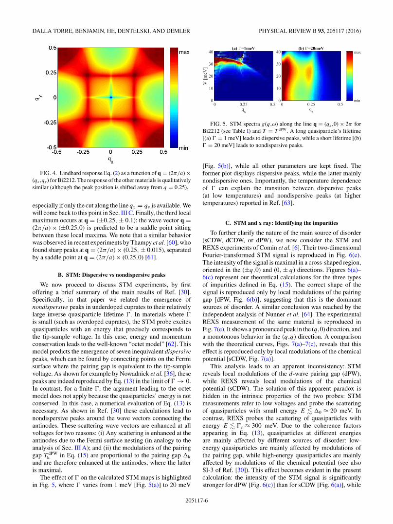
FIG. 5. STM spectra g(q,ω) along the line q = (qx,0) × 2π forBi2212 (see Table I) and T = T dPW. A long quasiparticle’s lifetime[(a) � = 1 meV] leads to dispersive peaks, while a short lifetime [(b)� = 20 meV] leads to nondispersive peaks.

[Fig. 5(b)], while all other parameters are kept fixed. Theformer plot displays dispersive peaks, while the latter mainlynondispersive ones. Importantly, the temperature dependenceof � can explain the transition between dispersive peaks(at low temperatures) and nondispersive peaks (at highertemperatures) reported in Ref. [63].

C. STM and x ray: Identifying the impurities

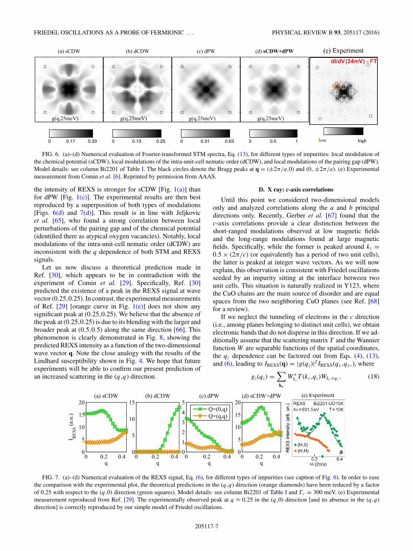
To further clarify the nature of the main source of disorder(sCDW, dCDW, or dPW), we now consider the STM andREXS experiments of Comin et al. [6]. Their two-dimensionalFourier-transformed STM signal is reproduced in Fig. 6(e).The intensity of the signal is maximal in a cross-shaped region,oriented in the (±q,0) and (0, ± q) directions. Figures 6(a)–6(c) represent our theoretical calculations for the three typesof impurities defined in Eq. (15). The correct shape of thesignal is reproduced only by local modulations of the pairinggap [dPW, Fig. 6(b)], suggesting that this is the dominantsources of disorder. A similar conclusion was reached by theindependent analysis of Nunner et al. [64]. The experimentalREXS measurement of the same material is reproduced inFig. 7(e). It shows a pronounced peak in the (q,0) direction, anda monotonous behavior in the (q,q) direction. A comparisonwith the theoretical curves, Figs. 7(a)–7(c), reveals that thiseffect is reproduced only by local modulations of the chemicalpotential [sCDW, Fig. 7(a)].

This analysis leads to an apparent inconsistency: STMreveals local modulations of the d-wave pairing gap (dPW),while REXS reveals local modulations of the chemicalpotential (sCDW). The solution of this apparent paradox ishidden in the intrinsic properties of the two probes: STMmeasurements refer to low voltages and probe the scatteringof quasiparticles with small energy E � �0 ≈ 20 meV. Incontrast, REXS probes the scattering of quasiparticles withenergy E � �c ≈ 300 meV. Due to the coherence factorsappearing in Eq. (13), quasiparticles at different energiesare mainly affected by different sources of disorder: low-energy quasiparticles are mainly affected by modulations ofthe pairing gap, while high-energy quasiparticles are mainlyaffected by modulations of the chemical potential (see alsoSI-3 of Ref. [30]). This effect becomes evident in the presentcalculation: the intensity of the STM signal is significantlystronger for dPW [Fig. 6(c)] than for sCDW [Fig. 6(a)], while

205117-6

FRIEDEL OSCILLATIONS AS A PROBE OF FERMIONIC . . . PHYSICAL REVIEW B 93, 205117 (2016)

g(q,25meV)

(a) sCDW

g(q,25meV)

(b) dCDW

g(q,25meV)

(c) dPW

g(q,25meV)

(d) sCDW+dPW

0 0.17 0.33 0 0.13 0.25 0 0.31 0.63 0 0.5 1

FIG. 6. (a)–(d) Numerical evaluation of Fourier-transformed STM spectra, Eq. (13), for different types of impurities: local modulation ofthe chemical potential (sCDW), local modulations of the intra-unit-cell nematic order (dCDW), and local modulations of the pairing gap (dPW).Model details: see column Bi2201 of Table I. The black circles denote the Bragg peaks at q = (±2π/a,0) and (0, ±2π/a). (e) Experimentalmeasurement from Comin et al. [6]. Reprinted by permission from AAAS.

the intensity of REXS is stronger for sCDW [Fig. 1(a)] thanfor dPW [Fig. 1(c)]. The experimental results are then bestreproduced by a superposition of both types of modulations[Figs. 6(d) and 7(d)]. This result is in line with Jeljkovicet al. [65], who found a strong correlation between localperturbations of the pairing gap and of the chemical potential(identified there as atypical oxygen vacancies). Notably, localmodulations of the intra-unit-cell nematic order (dCDW) areinconsistent with the q dependence of both STM and REXSsignals.

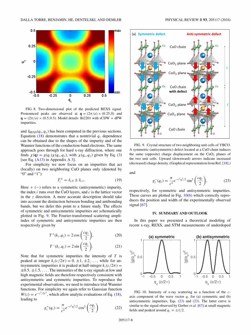
Let us now discuss a theoretical prediction made inRef. [30], which appears to be in contradiction with theexperiment of Comin et al. [29]. Specifically, Ref. [30]predicted the existence of a peak in the REXS signal at wavevector (0.25,0.25). In contrast, the experimental measurementsof Ref. [29] [orange curve in Fig. 1(e)] does not show anysignificant peak at (0.25,0.25). We believe that the absence ofthe peak at (0.25,0.25) is due to its blending with the larger andbroader peak at (0.5,0.5) along the same direction [66]. Thisphenomenon is clearly demonstrated in Fig. 8, showing thepredicted REXS intensity as a function of the two-dimensionalwave vector q. Note the close analogy with the results of theLindhard susceptibility shown in Fig. 4. We hope that futureexperiments will be able to confirm our present prediction ofan increased scattering in the (q,q) direction.

D. X ray: c-axis correlations

Until this point we considered two-dimensional modelsonly and analyzed correlations along the a and b principaldirections only. Recently, Gerber et al. [67] found that thec-axis correlations provide a clear distinction between theshort-ranged modulations observed at low magnetic fieldsand the long-range modulations found at large magneticfields. Specifically, while the former is peaked around kz =0.5 × (2π/c) (or equivalently has a period of two unit cells),the latter is peaked at integer wave vectors. As we will nowexplain, this observation is consistent with Friedel oscillationsseeded by an impurity sitting at the interface between twounit cells. This situation is naturally realized in Y123, wherethe CuO chains are the main source of disorder and are equalspaces from the two neighboring CuO planes (see Ref. [68]for a review).

If we neglect the tunneling of electrons in the c direction(i.e., among planes belonging to distinct unit cells), we obtainelectronic bands that do not disperse in this direction. If we ad-ditionally assume that the scattering matrix T and the Wannierfunction W are separable functions of the spatial coordinates,the qz dependence can be factored out from Eqs. (4), (13),and (6), leading to IREXS(q) = |g(qz)|2IREXS(qx,qy,), where

gz(qz) =∑

kz

W ∗kzT (kz,qz)Wkz+qz

, (18)

0 0.2 0.40

5

10

15

20

q

I REX

S (a.u

.)

(a) sCDW

0 0.2 0.40

5

10

15

q

(b) dCDW

0 0.2 0.40

1

2

3

4

5

q

(c) dPW

0 0.2 0.40

5

10

15

20

q

(d) sCDW+dPW

Q=(0,q)Q=(q,q)

FIG. 7. (a)–(d) Numerical evaluation of the REXS signal, Eq. (6), for different types of impurities (see caption of Fig. 6). In order to easethe comparison with the experimental plot, the theoretical predictions in the (q,q) direction (orange diamonds) have been reduced by a factorof 0.25 with respect to the (q,0) direction (green squares). Model details: see column Bi2201 of Table I and �c = 300 meV. (e) Experimentalmeasurement reproduced from Ref. [29]. The experimentally observed peak at q ≈ 0.25 in the (q,0) direction [and its absence in the (q,q)direction] is correctly reproduced by our simple model of Friedel oscillations.

205117-7

DALLA TORRE, BENJAMIN, HE, DENTELSKI, AND DEMLER PHYSICAL REVIEW B 93, 205117 (2016)

FIG. 8. Two-dimensional plot of the predicted REXS signal.Pronounced peaks are observed at q = (2π/a) × (0.25,0) andq = (2π/a) × (0.5,0.5). Model details: Bi2201 with sCDW + dPWimpurities.

and IREXS(qx,qy) has been computed in the previous sections.Equation (18) demonstrates that a nontrivial qz dependencecan be obtained due to the shapes of the impurity and of theWannier functions of the conduction-band electrons. The sameapproach goes through for hard x-ray diffraction, where onefinds χ (q) = g(qz)χ (qx,qy), with χ (qx,qy) given by Eq. (3)[see Eq. (A13) in Appendix A 3].

For simplicity we now focus on an impurities that act(locally) on two neighboring CuO planes only (denoted by“0” and “1”):

T ±i = δi,0 ± δi,1. (19)

Here + (−) refers to a symmetric (antisymmetric) impurity,the index i runs over the CuO layers, and c is the lattice vectorin the z direction. A more accurate description should takeinto account the distinction between bonding and antibondingbands, but we defer this point to a future study. The effectsof symmetric and antisymmetric impurities are schematicallyplotted in Fig. 9. The Fourier-transformed scattering ampli-tudes of symmetric and antisymmetric impurities are thenrespectively given by

T +(kz,qz) = 2 cos

(cqz

2

), (20)

T −(kz,qz) = 2 sin

(cqz

2

). (21)

Note that for symmetric impurities the intensity of T ispeaked at integer kz(c/2π ) = 0, ±1, ±2, . . . , while for an-tisymmetric impurities it is peaked at half-integer kz(c/2π ) =±0.5, ±1.5, . . . . The intensities of the x-ray signals at low andhigh magnetic fields are therefore respectively consistent withantisymmetric and symmetric impurities. To reproduce theexperimental observations, we need to introduce trial Wannierfunctions. For simplicity we again refer to Gaussian functionW (z) = e−z2/2c2

, which allow analytic evaluations of Eq. (18),leading to

g+z (qz) = π

c2e−c2q2

z /2 cos2

(cqz

2

)(22)

FIG. 9. Crystal structure of two neighboring unit cells of YBCO.A symmetric (antisymmetric) defect located at a CuO chain inducesthe same (opposite) charge displacement on the CuO2 planes ofthe two unit cells. Upward (downward) arrows indicate increased(decreased) charge density. (Graphical representation from Ref. [18].)

and

g−z (qz) = π

c2e−c2q2

z /2 sin2

(cqz

2

), (23)

respectively, for symmetric and antisymmetric impurities.These curves are plotted in Fig. 10(b) which correctly repro-duces the position and width of the experimentally observedsignal [67].

IV. SUMMARY AND OUTLOOK

In this paper we presented a theoretical modeling ofrecent x-ray, REXS, and STM measurements of underdoped

qz (c/2π)

-1 -0.5 0 0.5 1

|g(q

z)|2

0

0.5

1(a) symmetric

qz (c/2π)

-1 -0.5 0 0.5 1

|g(q

z)|2

0

0.5

1(b) antisymmetric

FIG. 10. Intensity of x-ray scattering as a function of the c-axis component of the wave vector qz for (a) symmetric and (b)antisymmetric impurities, Eqs. (23) and (23). The latter curve issimilar to the signal observed by Gerber et al. [67] at small magneticfields and peaked around qz = ±1/2.

205117-8

FRIEDEL OSCILLATIONS AS A PROBE OF FERMIONIC . . . PHYSICAL REVIEW B 93, 205117 (2016)

cuprates, with specific attention to Ghiringhelli et al. [4],Chang et al. [5], and Comin et al. [29]. To interpret theirexperimental findings, these authors assumed the existenceof a competing order, distinct from superconductivity, andassociated with the spontaneous breaking of translationalsymmetry. The pseudogap energy scale could then correspondto the excitation gap required to restore the translationalinvariance. The association between the charge ordering andthe pseudogap phase is however undermined by recent x-rayexperiments revealing the same type of charge ordering inelectron-doped cuprates [69], where a pseudogap phase is notexpected to subsist. In addition, the experiment by Gerberet al. [67] showed that the oscillations observed at smallmagnetic fields have different c-axis correlations than thoseobserved at large magnetic field [67], indicating that these aretwo distinct effects. Similarly, recent measurements of the Hallconductivity [70] show that long-range-ordered modulationsappear only for magnetic fields that are larger than a criticalvalue Hc ≈ 20 T.

Following Ref. [30] we propose here that the modulationsobserved at small magnetic fields are simply due to Friedeloscillations around local sources of disorder. Because ourinterpretation is based on the Born approximation (first-orderperturbation theory in the impurity strength) and we considereach scatterer independently, we expect the correlation lengthof the modulations to be independent on the concentration ofimpurities. This prediction has been now confirmed by twoexperimental observations: (i) Achkar et al. [71] modified theamount of disorder in Y123 through a thermal quench andobserved that the correlation length of the observed oscillationswas unchanged. (ii) The analysis of materials with similarband structure and different amount of intrinsic disorder (suchas Bi2201 [6,7], Bi2212 [8], and Hg1201 [9]) revealed anapproximately constant correlation length. These findings arenot consistent with theories of competing orders, in which thepredicted correlation length should be directly related to theamount of external disorder [72].

By considering the scattering of short-lived quasiparticlesfrom local impurities, we can quantitatively reproduce all theexperimental findings: Our model correctly predicts the wavevector and correlation length of the spatial modulations thatwere observed in x-ray [Figs. 3(b) and 4], STM (Fig. 5),and REXS (Fig. 7) experiments. The wave vector is similar(but not identical) to the distance between adjacent antinodes,where the Fermi surface is often quite nested. Our approachreproduces experimental observations that were interpretedas evidence for the d-wave symmetry of the oscillations(Fig. 7, see also Ref. [35] for an in-depth analysis of the phasecorrelations observed by Fujita et al. [10]). Finally, it naturallyaccounts for the nontrivial c-axis correlations observed in x-rayexperiments (Fig. 10).

To reproduce the experimental results, we introduceddifferent models of local impurities and found that themost dominant type corresponds to local modulations ofthe chemical potential and of the pairing gap. In STM maps,the former contribution is generically dominant along the(q,q) direction, while the latter is dominant along the (0,q)direction (see Fig. 6). The interplay between these two sourcesof disorder connects to the earlier analysis of STM data in thepresence of a magnetic field performed by Hanaguri et al. [73]

T

p

H

SC

PG

CDW

T

HSC

PG

CDW

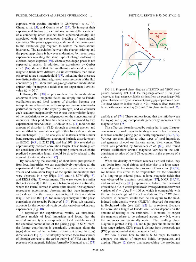
FIG. 11. Proposed phase diagram of BSCCO and YBCO com-pounds, following Ref. [76]: the long-range-ordered CDW phaseobserved at high magnetic field is distinct from the pseudogap (PG)phase, characterized by an incoherent pairing gap of preformed pairs.The inset refers to doping levels p ≈ 0.1, where a direct transitionbetween the superconducting (SC) and CDW phases is observed [76].

and He et al. [74]. These authors found that the ratio betweenthe (q,q) and (0,q) components generically increases withmagnetic field [75].

This effect can be understood by noting that in type-II super-conductors external magnetic fields generate isolated vortices,in whose core the pairing gap is locally suppressed [19,78,79].Vortices are then similar to other types of local impurities,and generate Friedel oscillations around their center. Thiseffect was predicted by Simonucci et al. [80], who foundFriedel oscillations around magnetic vortices in the self-consistent solution of the BCS equations in the presence of avortex.

When the density of vortices reaches a critical value, theycan depin from local defects and give rise to a long-range-ordered phase. Following the proposal of Wu et al. [19,79],we believe this effect to be responsible for the formationof a long-range-ordered phase at large magnetic fields thatwas observed by quantum oscillations [17], NMR [19,79],and sound velocity [81] experiments. Indeed, the measuredcritical field ∼20T corresponds to an average distance betweenvortices of d = √

φ0/B ∼ 100 A, which is comparable withthe correlation length of Friedel oscillations. The CDW phaseobserved in cuprates would then be analogous to the field-induced spin density waves (FISDW) observed for examplein Bechgaard salts (see Ref. [82] for a review). Becausethe correlation length of Friedel oscillations depends on theamount of nesting at the antinodes, it is natural to expectthe magnetic phase to be enhanced around p = 0.1, wherethe antinodes are maximally nested. The resulting phasediagram is plotted in Fig. 11, and highlights our claim that thelong-range ordered CDW phase is distinct from the pseudogap(PG) phase observed at zero magnetic field.

We now discuss how to utilize STM maps to furthercompare the effects of magnetic fields, temperature, anddoping. Figure 12 shows that approaching the pseduogap

205117-9

DALLA TORRE, BENJAMIN, HE, DENTELSKI, AND DEMLER PHYSICAL REVIEW B 93, 205117 (2016)

(a) small H

(b) large H (d) large T (f) small p (h) dominant direction

(c) small T (e) large p (g) dominant direction

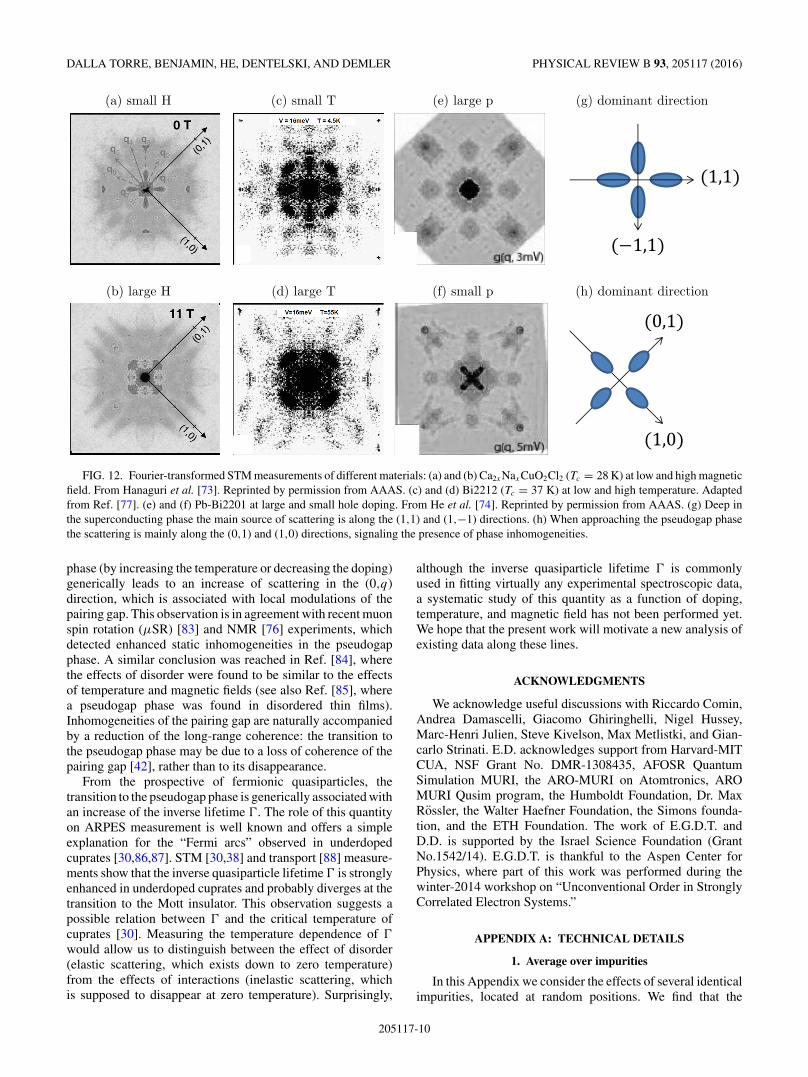
FIG. 12. Fourier-transformed STM measurements of different materials: (a) and (b) Ca2xNaxCuO2Cl2 (Tc = 28 K) at low and high magneticfield. From Hanaguri et al. [73]. Reprinted by permission from AAAS. (c) and (d) Bi2212 (Tc = 37 K) at low and high temperature. Adaptedfrom Ref. [77]. (e) and (f) Pb-Bi2201 at large and small hole doping. From He et al. [74]. Reprinted by permission from AAAS. (g) Deep inthe superconducting phase the main source of scattering is along the (1,1) and (1,−1) directions. (h) When approaching the pseudogap phasethe scattering is mainly along the (0,1) and (1,0) directions, signaling the presence of phase inhomogeneities.

phase (by increasing the temperature or decreasing the doping)generically leads to an increase of scattering in the (0,q)direction, which is associated with local modulations of thepairing gap. This observation is in agreement with recent muonspin rotation (μSR) [83] and NMR [76] experiments, whichdetected enhanced static inhomogeneities in the pseudogapphase. A similar conclusion was reached in Ref. [84], wherethe effects of disorder were found to be similar to the effectsof temperature and magnetic fields (see also Ref. [85], wherea pseudogap phase was found in disordered thin films).Inhomogeneities of the pairing gap are naturally accompaniedby a reduction of the long-range coherence: the transition tothe pseudogap phase may be due to a loss of coherence of thepairing gap [42], rather than to its disappearance.

From the prospective of fermionic quasiparticles, thetransition to the pseudogap phase is generically associated withan increase of the inverse lifetime �. The role of this quantityon ARPES measurement is well known and offers a simpleexplanation for the “Fermi arcs” observed in underdopedcuprates [30,86,87]. STM [30,38] and transport [88] measure-ments show that the inverse quasiparticle lifetime � is stronglyenhanced in underdoped cuprates and probably diverges at thetransition to the Mott insulator. This observation suggests apossible relation between � and the critical temperature ofcuprates [30]. Measuring the temperature dependence of �

would allow us to distinguish between the effect of disorder(elastic scattering, which exists down to zero temperature)from the effects of interactions (inelastic scattering, whichis supposed to disappear at zero temperature). Surprisingly,

although the inverse quasiparticle lifetime � is commonlyused in fitting virtually any experimental spectroscopic data,a systematic study of this quantity as a function of doping,temperature, and magnetic field has not been performed yet.We hope that the present work will motivate a new analysis ofexisting data along these lines.

ACKNOWLEDGMENTS

We acknowledge useful discussions with Riccardo Comin,Andrea Damascelli, Giacomo Ghiringhelli, Nigel Hussey,Marc-Henri Julien, Steve Kivelson, Max Metlistki, and Gian-carlo Strinati. E.D. acknowledges support from Harvard-MITCUA, NSF Grant No. DMR-1308435, AFOSR QuantumSimulation MURI, the ARO-MURI on Atomtronics, AROMURI Qusim program, the Humboldt Foundation, Dr. MaxRossler, the Walter Haefner Foundation, the Simons founda-tion, and the ETH Foundation. The work of E.G.D.T. andD.D. is supported by the Israel Science Foundation (GrantNo.1542/14). E.G.D.T. is thankful to the Aspen Center forPhysics, where part of this work was performed during thewinter-2014 workshop on “Unconventional Order in StronglyCorrelated Electron Systems.”

APPENDIX A: TECHNICAL DETAILS

1. Average over impurities

In this Appendix we consider the effects of several identicalimpurities, located at random positions. We find that the

205117-10

FRIEDEL OSCILLATIONS AS A PROBE OF FERMIONIC . . . PHYSICAL REVIEW B 93, 205117 (2016)

absolute value of g(q,ω) is independent on their position andtherefore is an intrinsic property of the system. In the text[Eq. (8)] we assumed g(r,ω) to be symmetric under r → −r.This approximation is valid in the presence of a single impuritylocated at the origin of the axis [89]. To extend this treatmentto systems with several impurities, we first notice that withinthe present framework (first-order perturbation theory in theimpurity strength) g(q �= G,ω) is given by a sum of terms,each referring to the scattering of quasiparticles from a singleimpurity: g(q,ω) = ∑

i gi(q,ω), where i runs over all theimpurities. To compute gi(q,ω) we first consider a coordinatesystem whose origin is located at the center of the ith impurity,where Eq. (13) applies. We then shift back gi(q,ω) to the com-mon laboratory frame by the multiplication with eiq·ri , and sumall the terms. In the case of N identical impurities we obtain

g(q,ω) =N∑

i=1

eiq·ri g0(q,ω). (A1)

Here g0(q,ω) is the scattering amplitude from an isolatedimpurity located at the axis origin, computed from Eq. (13).In Eq. (A1) the phase of g(q,ω) is determined by the randompositions ri and is therefore not predictable. In contrast, itsabsolute value averages to

〈|g(q,ω)|〉 = Ng0(q,ω). (A2)

Here we used the observation that by definition, g0(q,ω) is areal function.

2. Green’s function approach to REXS

In this Appendix we derive Eq. (6) within the Keldyshpath-integral formalism. This approach allows us to extendthe results of Abbamonte et al. [27] to finite temperatures.In REXS experiments x rays are scattered upon the materialto be examined at a frequency that allows the creation of acore hole, i.e., the excitation of an inner orbital of the atom tothe conduction band (see Fig. 1). The action of the incomingfield can be described as Vin = Eine

iωt δ(t)d†c + H.c., whereEin > 0 describes the amplitude of the incoming x rays, withω its frequency, and d and c are fermionic operators describingelectrons (quasiparticles), respectively, in the conduction band(in cuprates formed by d orbitals) and in the core level. Shortlyafter, an electron from the conduction band fills in the corelevel and emits an x-ray photon, which is observed by theexperimental setup. This decay process can be described by theoperator Vout(t) = a

†oute

−iωt c†d, where a†out creates an outgoing

photon and λ is the light-matter coupling. In perturbationtheory, the outgoing field is given by

Eout(t) = 〈aout〉 ≈ 〈c†de−iωt + H.c.〉, (A3)

where we assumed the initial state to be empty of outgoingphotons. Applying perturbation theory (and neglecting oscil-lating terms), we obtain the Kubo formula

Eout(t) = iEin�(t)〈[d†(0)c(0),c†(t)d(t)]〉, (A4)

where �(t) is the Heaviside theta function and [. . . , . . . ] is thecommutation relation. In Keldysh notation, Eq. (A4) becomesthe sum of eight terms with an odd number of “classical”fields c,d and of “quantum” fields c,d . Four of these terms

contain three quantum fields and their expectation values areidentically equal to zero. We are then left only with termscontaining three classical fields and one quantum field:

Eout(t) = i

2Ein�(t)〈d∗(0)c(0)c∗(t)d(t)

+d∗(0)c(0)c∗(t)d(t) + d∗(0)c(0)c∗(t)d(t)

+d∗(0)c(0)c∗(t)d(t)〉. (A5)

For t > 0 only the first two terms are nonzero (and for t < 0 thelast two are nonzero). Equation (A5) can be further simplifiedby introducing the retarded and Keldysh Green’s functionsGR

d = 〈d∗d〉 and GKd = 〈d∗d〉:

Eout = iEin[GK

d (t)GRc (t) + GK

c (t)GRd (t)

]. (A6)

Each of the two terms of Eq. (A6) corresponds to the productof two Greens functions, evaluated at the same time, orequivalently their convolution in the frequency domain:

Eout(ω) = i

2Ein

∫ ∞

−∞dω′[GK

d (ω − ω′)GRc (ω′)

+GKc (ω′)GR

d (ω − ω′)]. (A7)

At thermal equilibrium the Keldysh components satisfythe fluctuation-dissipation theorem GK

d (ω) = 2Im[GRd ] tanh

(ω/2T ) ≈ 2Im[GRd ]sgn(ω) and GK

c =2Im[GRc ] tanh((ω −

Eh)/2T ) ≈ −2Im[GRc ]. In the limit of T → 0 we find

Eout(ω) = iEin

∫ ∞

−∞dω′[Im[

GRc

](ω − ω′)GR

d (ω′)

+ sgn(ω′)Im[GR

d

](ω′)GR

c (ω − ω′)]. (A8)

The real component of Eout (the component that is in phasewith Ein) has a particularly simple form

Re[Eout](ω) = 2Ein

∫ ∞

0dω′Im

[GR

c

](ω − ω′)Im

[GR

d (ω′)].

(A9)Applying the Karmers-Kronig relation we then obtain

Eout(ω) = 2Ein

∫ ∞

0dω′GR

c (ω − ω′)Im[GR

d (ω′)]. (A10)

For a featureless core level with response function GRc (q,ω) =

[(ω + i�c)]−1, we recover exactly the same expression as inRef. [27] and Eq. (6) with A = 2Ein.

3. From REXS to Lindhard

In the main text we provided an expression for the intensityof the REXS signal at zero temperature, Eq. (6). Here we showthat, in the case of nonresonant scattering from a Fermi gas, thisexpression simply reduces to the Lindhard susceptibility (2).The present derivation is a corollary of a more genericrelation between the nonresonant limit of resonant inelasticscattering (RIXS) and density-density response functions (seeRef. [28] for a review), and is brought here for completeness.Nonresonant scattering can be described as a REXS processin the limit of �c → ∞. In a Fermi gas with a local impurity,G0(k,ω) = 1/(ω−εk + i0+), W (k) = 1, and T (k,k + q) = 1.Under these conditions Eqs. (6) and (8) give IREXS → Ix ray =

205117-11

DALLA TORRE, BENJAMIN, HE, DENTELSKI, AND DEMLER PHYSICAL REVIEW B 93, 205117 (2016)

|(AC(q)/�c|2, with

C(q) =∫ ∞

0dω′ ∑

k

Im

[1

ω′ − εk + i0+1

ω′ − εk+q + i0+

]

= π

∫ ∞

0dω′ ∑

k

δ(ω′ − εk+q)

ω′ − εk+ δ(ω′ − εk)

ω′ − εk+q

= π

∫ ∞

0dω′ ∑

k

δ(ω′ − εk+q)

εk+q − εk+ δ(ω′ − εk)

εk − εk+q

= π∑

k

nk

εk+q − εk+ nk+q

εk − εk+q. (A11)

Here in the transition from the first to the second line we used1/(x + i0+) = 1/x − iπδ(x), and in the transition from thethird to fourth

∫ ∞0 δ(ω − εk) = nk , where nk is the Fermi-Dirac

distribution at T = 0. We obtain

Ix ray =∣∣∣∣∣A

�c

∑k

nk − nk+q

εk − εk+q

∣∣∣∣∣2

=∣∣∣∣ A

�c

χ (q)

∣∣∣∣2

. (A12)

The present derivation can be extended to the case of nontrivialWannier functions, and scattering amplitudes of the formT (k,k + q) = Tq leading to

Ix ray =∣∣∣∣∣A

�c

∑k

WkTqW∗k+q

nk − nk+q

εk − εk+q

∣∣∣∣∣2

. (A13)

4. Spin-orbit effects in REXS

In this Appendix we study the dependence of REXS scatteringon the polarization of the incoming (i) and outgoing (o)photons. As an important result, we will show that in theabsence of magnetic impurities, the intensity of the REXSsignal is not affected by spin-orbit effects. For an isolatedatom, the REXS intensity I is given by the product of dipolematrix elements for the absorption and the emission:

I (ηi ,ηo) ∝ (η∗o · 〈ψi |r|ψn〉)(ηi · 〈ψn|r|ψi〉), (A14)

where ψi is the initial (and final) core electron state andψn is a valence 3dx2−y2 orbital with spin σ at the samesite. In typical experiments one selects a resonance so thatonly 2p core levels with total angular momentum j = 3/2are excited to the valence band. Thus the total polarization-dependent intensity is the sum over spin-orbit eigenstatesmj = −3/2, − 1/2,1/2,3/2:

I (ηi ,ηo) ∝∑mj

(η∗

o · ⟨2p3/2

mj|r|3dx2−y2 ,σ

⟩)

× (ηi · ⟨

3dx2−y2 ,σ |r|2p3/2mj

⟩). (A15)

To compute the dipole matrix elements, we introduce a unitoperator in the basis of separate spin and orbital angular-momentum eigenstates |m�,ms〉,

I ∝∑

mj ,m�,ms,m′�,m

′s

(η∗

o · ⟨2p3/2

mj

∣∣m�,ms

⟩⟨m�,ms |r|3dx2−y2 ,σ

⟩)

× (ηi · ⟨

3dx2−y2 ,σ |r|m′�,m

′s

⟩⟨m′

�,m′s

∣∣2p3/2mj

⟩)(A16)

=∑

mj ,m�,m′�

(η∗

o · ⟨2p3/2

mj

∣∣m�,σ⟩⟨m�|r|3dx2−y2

⟩)

× (ηi · ⟨

3dx2−y2 |r|m′�

⟩⟨m′

�,σ |2p3/2mj

⟩). (A17)

The Clebsch-Gordan matrix elements vanish unless mj =m� + σ = m′

� + σ , and hence we require m′� = m�. We then

have the further simplification:

I ∝∑

mj ,m�

∣∣⟨2p3/2mj

∣∣m�,σ⟩∣∣2

(η∗o · 〈m�|r|3dx2−y2〉)

×(ηi · 〈3dx2−y2 |r|m�〉). (A18)

If the Hamiltonian is spin independent, i.e., if there is nospin-density wave, the amplitude is independent of the spin σ

of the photoelectron in the intermediate state and thus the twospins contribute equally to the coherent sum over histories,and we have

I ∝∑m�

⎡⎣∑

mj ,σ

∣∣⟨2p3/2mj

∣∣m�,σ⟩∣∣2

⎤⎦(η∗

o · 〈m�|r|3dx2−y2〉)

×(ηi · 〈3dx2−y2 |r|m�〉). (A19)

Now∑

mj ,σ|〈2p

3/2mj

|m�,σ 〉|2 is the probability that a coreelectron with orbital angular momentum m� and unknown spinis in a total spin-j = 3/2 state. By spherical symmetry this isobviously independent of m�, since m� is coordinate dependentbut j is not. Since this is an m�-independent quantity, we obtain

I ∝∑m�

(η∗o · 〈m�|r|3dx2−y2〉)(ηi · 〈3dx2−y2 |r|m�〉) (A20)

=〈3dx2−y2 |(ηi · r)(η∗o · r)|3dx2−y2〉. (A21)

We now have a tensorial matrix element that is not modulatedby the spin-orbit effect except for the aforementioned constantprefactor that represents the contribution to resonant scatteringonly from j = 3/2 core states.

5. Polarization dependence of REXS

In this Appendix we study the dependence of the REXSsignal on the wavevector of the incoming photon k. This de-pendence was experimentally measured by Comin et al. [29],and used to identify the dominant type of charge modulations.According to the present single-band approach, the predictedk dependence is instead identical for all types of modulations:Our model corresponds to the s-wave case considered byComin et al. This model is found to be in good agreementwith the experimental measurements (see Fig. 14).

Our starting point is Eq. (7). Because the outgoing beam isnot filtered according to its polarization, the measured signalis proportional to the sum of the intensities of the two outgoingpolarizations:

IREXS ∝∑

o=σ ′,π ′|ηo · M · ηi |2, (A22)

where the tensor M is defined by Mα,β = 〈d|rαrβ |d〉, i = σ,π

is the incoming polarization, and o = σ ′,π ′ is the outgoingpolarization. We denote by F the diagonal matrix correspond-ing to M in the principal axis of the lattice. Its three nonzero

205117-12

FRIEDEL OSCILLATIONS AS A PROBE OF FERMIONIC . . . PHYSICAL REVIEW B 93, 205117 (2016)

o

xyxqz

x

sample

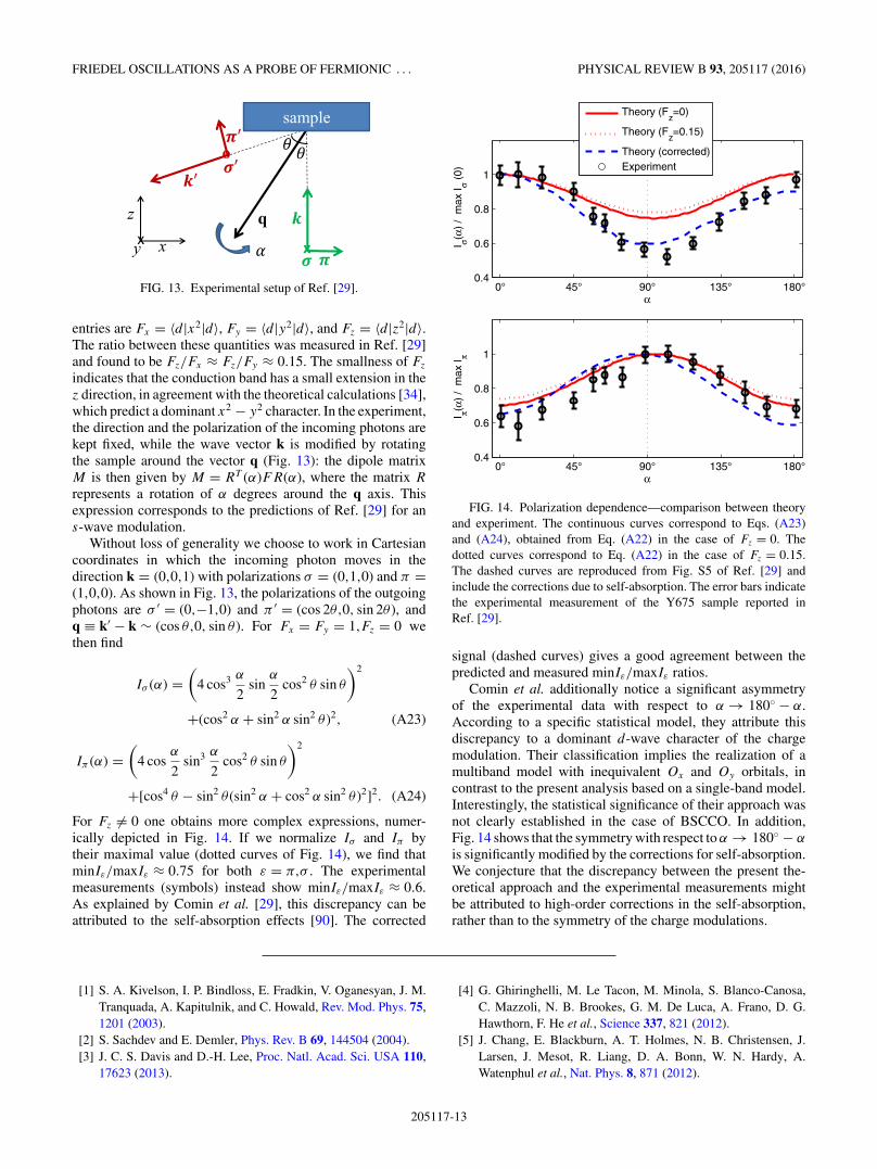
FIG. 13. Experimental setup of Ref. [29].

entries are Fx = 〈d|x2|d〉, Fy = 〈d|y2|d〉, and Fz = 〈d|z2|d〉.The ratio between these quantities was measured in Ref. [29]and found to be Fz/Fx ≈ Fz/Fy ≈ 0.15. The smallness of Fz

indicates that the conduction band has a small extension in thez direction, in agreement with the theoretical calculations [34],which predict a dominant x2 − y2 character. In the experiment,the direction and the polarization of the incoming photons arekept fixed, while the wave vector k is modified by rotatingthe sample around the vector q (Fig. 13): the dipole matrixM is then given by M = RT (α)FR(α), where the matrix R

represents a rotation of α degrees around the q axis. Thisexpression corresponds to the predictions of Ref. [29] for ans-wave modulation.

Without loss of generality we choose to work in Cartesiancoordinates in which the incoming photon moves in thedirection k = (0,0,1) with polarizations σ = (0,1,0) and π =(1,0,0). As shown in Fig. 13, the polarizations of the outgoingphotons are σ ′ = (0,−1,0) and π ′ = (cos 2θ,0, sin 2θ ), andq ≡ k′ − k ∼ (cos θ,0, sin θ ). For Fx = Fy = 1,Fz = 0 wethen find

Iσ (α) =(

4 cos3 α

2sin

α

2cos2 θ sin θ

)2

+(cos2 α + sin2 α sin2 θ )2, (A23)

Iπ (α) =(

4 cosα

2sin3 α

2cos2 θ sin θ

)2

+[cos4 θ − sin2 θ (sin2 α + cos2 α sin2 θ )2]2. (A24)

For Fz �= 0 one obtains more complex expressions, numer-ically depicted in Fig. 14. If we normalize Iσ and Iπ bytheir maximal value (dotted curves of Fig. 14), we find thatminIε/maxIε ≈ 0.75 for both ε = π,σ . The experimentalmeasurements (symbols) instead show minIε/maxIε ≈ 0.6.As explained by Comin et al. [29], this discrepancy can beattributed to the self-absorption effects [90]. The corrected

0° 45° 90° 135° 180°0.4

0.6

0.8

1

α

I σ(α)

/ m

ax I σ (

0)0° 45° 90° 135° 180°

0.4

0.6

0.8

1

I π(α)

/ m

ax I π

α

Theory (Fz=0)

Theory (Fz=0.15)

Theory (corrected)Experiment

FIG. 14. Polarization dependence—comparison between theoryand experiment. The continuous curves correspond to Eqs. (A23)and (A24), obtained from Eq. (A22) in the case of Fz = 0. Thedotted curves correspond to Eq. (A22) in the case of Fz = 0.15.The dashed curves are reproduced from Fig. S5 of Ref. [29] andinclude the corrections due to self-absorption. The error bars indicatethe experimental measurement of the Y675 sample reported inRef. [29].

signal (dashed curves) gives a good agreement between thepredicted and measured minIε/maxIε ratios.

Comin et al. additionally notice a significant asymmetryof the experimental data with respect to α → 180◦ − α.According to a specific statistical model, they attribute thisdiscrepancy to a dominant d-wave character of the chargemodulation. Their classification implies the realization of amultiband model with inequivalent Ox and Oy orbitals, incontrast to the present analysis based on a single-band model.Interestingly, the statistical significance of their approach wasnot clearly established in the case of BSCCO. In addition,Fig. 14 shows that the symmetry with respect to α → 180◦ − α

is significantly modified by the corrections for self-absorption.We conjecture that the discrepancy between the present the-oretical approach and the experimental measurements mightbe attributed to high-order corrections in the self-absorption,rather than to the symmetry of the charge modulations.

[1] S. A. Kivelson, I. P. Bindloss, E. Fradkin, V. Oganesyan, J. M.Tranquada, A. Kapitulnik, and C. Howald, Rev. Mod. Phys. 75,1201 (2003).

[2] S. Sachdev and E. Demler, Phys. Rev. B 69, 144504 (2004).[3] J. C. S. Davis and D.-H. Lee, Proc. Natl. Acad. Sci. USA 110,

17623 (2013).

[4] G. Ghiringhelli, M. Le Tacon, M. Minola, S. Blanco-Canosa,C. Mazzoli, N. B. Brookes, G. M. De Luca, A. Frano, D. G.Hawthorn, F. He et al., Science 337, 821 (2012).

[5] J. Chang, E. Blackburn, A. T. Holmes, N. B. Christensen, J.Larsen, J. Mesot, R. Liang, D. A. Bonn, W. N. Hardy, A.Watenphul et al., Nat. Phys. 8, 871 (2012).

205117-13

DALLA TORRE, BENJAMIN, HE, DENTELSKI, AND DEMLER PHYSICAL REVIEW B 93, 205117 (2016)

[6] R. Comin, A. Frano, M. M. Yee, Y. Yoshida, H. Eisaki, E.Schierle, E. Weschke, R. Sutarto, F. He, A. Soumyanarayananet al., Science 343, 390 (2014).

[7] E. H. da Silva Neto, P. Aynajian, A. Frano, R. Comin, E. Schierle,E. Weschke, A. Gyenis, J. Wen, J. Schneeloch, Z. Xu et al.,Science 343, 393 (2014).

[8] M. Hashimoto, G. Ghiringhelli, W.-S. Lee, G. Dellea, A.Amorese, C. Mazzoli, K. Kummer, N. B. Brookes, B. Moritz,Y. Yoshida et al., Phys. Rev. B 89, 220511(R) (2014).

[9] W. Tabis, Y. Li, M. L. Tacon, L. Braicovich, A. Kreyssig, M.Minola, G. Dellea, E. Weschke, M. J. Veit, M. Ramazanogluet al., Nat. Commun. 5, 5875 (2014).

[10] K. Fujita, M. H. Hamidian, S. D. Edkins, C. K. Kim, Y. Kohsaka,M. Azuma, M. Takano, H. Takagi, H. Eisaki, S.-i. Uchida et al.,Proc. Natl. Acad. Sci. USA 111, E3026 (2014).

[11] M. H. Hamidian, S. D. Edkins, C. K. Kim, J. C. Davis, A. P.Mackenzie, H. Eisaki, S. Uchida, M. J. Lawler, E.-A. Kim, S.Sachdev, and K. Fujita, Nat. Phys. 12, 150 (2016).

[12] M. H. Hamidian, S. D. Edkins, K. Fujita, A. Kostin, A. P.Mackenzie, H. Eisaki, S. Uchida, M. J. Lawler, E.-A. Kim,S. Sachdev, and J. C. S. Davis, arXiv:1508.00620.

[13] J. E. Hoffman, E. W. Hudson, K. M. Lang, V. Madhavan,H. Eisaki, S. Uchida, and J. C. Davis, Science 295, 466(2002).

[14] C. Howald, H. Eisaki, N. Kaneko, M. Greven, and A. Kapitulnik,Phys. Rev. B 67, 014533 (2003).

[15] T. Hanaguri, C. Lupien, Y. Kohsaka, D.-H. Lee, M. Azuma, M.Takano, H. Takagi, and J. C. Davis, Nature (London) 430, 1001(2004).

[16] M. Vershinin, S. Misra, S. Ono, Y. Abe, Y. Ando, and A. Yazdani,Science 303, 1995 (2004).

[17] N. Doiron-Leyraud, C. Proust, D. LeBoeuf, J. Levallois, J.-B.Bonnemaison, R. Liang, D. Bonn, W. Hardy, and L. Taillefer,Nature (London) 447, 565 (2007).

[18] N. Barisic, S. Badoux, M. K. Chan, C. Dorow, W. Tabis, B.Vignolle, G. Yu, J. Beard, X. Zhao, C. Proust et al., Nat. Phys.9, 761 (2013).

[19] T. Wu, H. Mayaffre, S. Kramer, M. Horvatic, C. Berthier, W. N.Hardy, R. Liang, D. A. Bonn, and M.-H. Julien, Nature (London)477, 191 (2011).

[20] E. G. Dalla Torre, D. Benjamin, Y. He, D. Dentelski, and E.Demler (unpublished).

[21] B. Mihaila, arXiv:1111.5337.[22] P. Sprunger, L. Petersen, E. Plummer, E. Lægsgaard, and F.

Besenbacher, Science 275, 1764 (1997).[23] L. Petersen, P. T. Sprunger, P. Hofmann, E. Lægsgaard, B. G.

Briner, M. Doering, H.-P. Rust, A. M. Bradshaw, F. Besenbacher,and E. W. Plummer, Phys. Rev. B 57, R6858 (1998).

[24] S. Rouziere, S. Ravy, J.-P. Pouget, and S. Brazovskii, Phys. Rev.B 62, R16231 (2000).

[25] N. D. M. N. W. Ashcroft, Solid State Physics (Saunders College,London, 1976).

[26] Note that current experiments would detect this situation as apronounced peak at q = 2kF due to the common practice of“background subtraction.”

[27] P. Abbamonte, E. Demler, J. S. Davis, and J.-C. Campuzano,Physica C 481, 15 (2012).

[28] L. J. Ament, M. van Veenendaal, T. P. Devereaux, J. P. Hill, andJ. van den Brink, Rev. Mod. Phys. 83, 705 (2011).

[29] R. Comin, R. Sutarto, F. He, E. da Silva Neto, L. Chauviere,A. Frano, R. Liang, W. Hardy, D. Bonn, Y. Yoshida et al.,Nat. Mater. 14, 796 (2015).

[30] E. G. Dalla Torre, Y. He, D. Benjamin, and E. Demler, New J.Phys. 17, 022001 (2015).

[31] D. Podolsky, E. Demler, K. Damle, and B. I. Halperin,Phys. Rev. B 67, 094514 (2003).

[32] P. Choubey, T. Berlijn, A. Kreisel, C. Cao, and P. J. Hirschfeld,Phys. Rev. B 90, 134520 (2014).

[33] A. Kreisel, P. Choubey, T. Berlijn, W. Ku, B. M. Andersen, andP. J. Hirschfeld, Phys. Rev. Lett. 114, 217002 (2015).

[34] F.C. Zhang and T.M. Rice, Phys. Rev. B 37, 3759 (1988).[35] E. G. Dalla Torre, Y. He, and E. Demler, arXiv:1512.03456.[36] E. A. Nowadnick, B. Moritz, and T. P. Devereaux, Phys. Rev. B

86, 134509 (2012).[37] S. Hufner, M. Hossain, A. Damascelli, and G. Sawatzky,

Rep. Prog. Phys. 71, 062501 (2008).[38] J. W. Alldredge, J. Lee, K. McElroy, M. Wang, K. Fujita, Y.

Kohsaka, C. Taylor, H. Eisaki, S. Uchida, P. J. Hirschfeld et al.,Nat. Phys. 4, 319 (2008).

[39] Y. J. Uemura, G. M. Luke, B. J. Sternlieb, J. H. Brewer, J. F.Carolan, W. N. Hardy, R. Kadono, J. R. Kempton, R. F. Kiefl,S. R. Kreitzman et al., Phys. Rev. Lett. 62, 2317 (1989).

[40] S. Doniach and M. Inui, Phys. Rev. B 41, 6668 (1990).[41] M. Randeria, N. Trivedi, A. Moreo, and R. T. Scalettar,

Phys. Rev. Lett. 69, 2001 (1992).[42] V. Emery and S. Kivelson, Nature (London) 374, 434

(1995).[43] Q. Chen, I. Kosztin, B. Janko, and K. Levin, Phys. Rev. Lett. 81,

4708 (1998).[44] M. Franz and A.J. Millis, Phys. Rev. B 58, 14572 (1998).[45] G. Deutscher, Nature (London) 397, 410 (1999).[46] H.-J. Kwon and A. T. Dorsey, Phys. Rev. B 59, 6438

(1999).[47] E. W. Carlson, S. A. Kivelson, V. J. Emery, and E. Manousakis,

Phys. Rev. Lett. 83, 612 (1999).[48] M. Lawler, K. Fujita, J. Lee, A. Schmidt, Y. Kohsaka, C. K. Kim,

H. Eisaki, S. Uchida, J. Davis, J. Sethna et al., Nature (London)466, 347 (2010).

[49] M. R. Norman, M. Randeria, H. Ding, and J. C. Campuzano,Phys. Rev. B 52, 615 (1995).

[50] M. C. Schabel, C.-H. Park, A. Matsuura, Z.-X. Shen, D. A.Bonn, X. Liang, and W. N. Hardy, Phys. Rev. B 57, 6090(1998).

[51] K. Pasanai and W. A. Atkinson, Phys. Rev. B 81, 134501(2010).

[52] P. D. C. King, J. A. Rosen, W. Meevasana, A. Tamai, E. Rozbicki,R. Comin, G. Levy, D. Fournier, Y. Yoshida, H. Eisaki et al.,Phys. Rev. Lett. 106, 127005 (2011).

[53] The antinodes are here defined as the points at which the Fermisurface reaches the boundaries of the first Brillouin zone.

[54] T. Kondo, T. Takeuchi, S. Tsuda, and S. Shin, Phys. Rev. B 74,224511 (2006).

[55] I. M. Vishik, M. Hashimoto, R.-H. He, W.-S. Lee, F. Schmitt,D. Lu, R. G. Moore, C. Zhang, W. Meevasana, T. Sasagawaet al., Proc. Natl. Acad. Sci. USA 109, 18332 (2012).

[56] Here we use the term “nesting” to indicate segments of the Fermisurface that are parallel to each other, leading to an enhancedscattering at the corresponding wavelength difference

205117-14

FRIEDEL OSCILLATIONS AS A PROBE OF FERMIONIC . . . PHYSICAL REVIEW B 93, 205117 (2016)

[57] M. Okawa, K. Ishizaka, H. Uchiyama, H. Tadatomo, T. Masui,S. Tajima, X.-Y. Wang, C.-T. Chen, S. Watanabe, A. Chainaniet al., Phys. Rev. B 79, 144528 (2009).

[58] M. Le Tacon, A. Bosak, S. Souliou, G. Dellea, T. Loew, R.Heid, K. Bohnen, G. Ghiringhelli, M. Krisch, and B. Keimer,Nat. Phys. 10, 52 (2014).

[59] D. Benjamin, D. Abanin, P. Abbamonte, and E. Demler,Phys. Rev. Lett. 110, 137002 (2013).

[60] V. Thampy, M. P. M. Dean, N. B. Christensen, L. Steinke, Z.Islam, M. Oda, M. Ido, N. Momono, S. B. Wilkins, and J. P.Hill, Phys. Rev. B 90, 100510 (2014).

[61] The quantitative discrepancy between our predictions andtheir finding may be attributed to either the different material(La1.88Sr0.12CuO4), or the different technique (resonant elasticx-ray scattering).

[62] Q.-H. Wang and D.-H. Lee, Phys. Rev. B 67, 020511 (2003).[63] C. V. Parker, P. Aynajian, E. H. da Silva Neto, A. Pushp, S. Ono,

J. Wen, Z. Xu, G. Gu, and A. Yazdani, Nature (London) 468,677 (2010).

[64] T. S. Nunner, W. Chen, B. M. Andersen, A. Melikyan, and P. J.Hirschfeld, Phys. Rev. B 73, 104511 (2006).

[65] I. Zeljkovic, Z. Xu, J. Wen, G. Gu, R. S. Markiewicz, and J. E.Hoffman, Science 337, 320 (2012).

[66] In the experimental curves reproduced in Fig. 1(e), the signalin (0,q) and (q,q) directions were normalized by a differentmultiplicative factor. Indeed, if the same normalization had beenused, the two curves should had converged in the q → 0 limit.As a consequence, the plot of Fig. 1(e) does not convey anyinformation about the ratio between the (0.25,0) and (0.25,0.25)wave vectors, but only describes the behavior of the REXSintensity in the (0,q) and (q,q) direction, independently.

[67] S. Gerber, H. Jang, H. Nojiri, S. Matsuzawa, H. Yasumura, D. A.Bonn, R. Liang, W. N. Hardy, Z. Islam, A. Mehta et al., Science350, 949 (2015).

[68] H. Alloul, J. Bobroff, M. Gabay, and P. Hirschfeld, Rev. Mod.Phys. 81, 45 (2009).

[69] E. H. da Silva Neto, R. Comin, F. He, R. Sutarto, Y. Jiang, R. L.Greene, G. A. Sawatzky, and A. Damascelli, Science 347, 282(2015).

[70] G. Grissonnanche, F. Laliberte, S. Dufour-Beausejour, A.Riopel, S. Badoux, M. Caouette-Mansour, M. Matusiak, A.Juneau-Fecteau, P. Bourgeois-Hope, O. Cyr-Choiniere et al.,arXiv:1508.05486.

[71] A. J. Achkar, X. Mao, C. McMahon, R. Sutarto, F. He, R. Liang,D. A. Bonn, W. N. Hardy, and D. G. Hawthorn, Phys. Rev. Lett.113, 107002 (2014).

[72] L. Nie, G. Tarjus, and S. A. Kivelson, Proc. Natl. Acad. Sci.USA 111, 7980 (2014).

[73] T. Hanaguri, Y. Kohsaka, M. Ono, M. Maltseva, P. Coleman,I. Yamada, M. Azuma, M. Takano, K. Ohishi, and H. Takagi,Science 323, 923 (2009).

[74] Y. He, Y. Yin, M. Zech, A. Soumyanarayanan, M. M. Yee, T.Williams, M. C. Boyer, K. Chatterjee, W. D. Wise, I. Zeljkovicet al., Science 344, 608 (2014).

[75] Because the wave vector (q,0) connects quasiparticles withopposite signs of the pairing gap, while the (q,q) wavevector connects quasiparticles with the same sign, these twocontributions are often referred to as “sign reversing” and “signpreserving.”

[76] T. Wu, H. Mayaffre, S. Kramer, M. Horvatic, C. Berthier, W. N.Hardy, R. Liang, D. A. Bonn, and M.-H. Julien, Nat. Commun.6, 6438 (2015).

[77] K. Fujita, A. R. Schmidt, E.-A. Kim, M. J. Lawler, D. H. Lee,J. C. Davis, H. Eisaki, and S.-i. Uchida, J. Phys. Soc. Jpn. 81,011005 (2012).

[78] T. Pereg-Barnea and M. Franz, Phys. Rev. B 68, 180506(2003).

[79] T. Wu, H. Mayaffre, S. Kramer, M. Horvatic, C. Berthier, P. L.Kuhns, A. P. Reyes, R. Liang, W. N. Hardy, D. A. Bonn et al.,Nat. Commun. 4, 2113 (2013).

[80] S. Simonucci, P. Pieri, and G. C. Strinati, Phys. Rev. B 87,214507 (2013).

[81] D. LeBoeuf, S. Kramer, W. Hardy, R. Liang, D. Bonn, andC. Proust, Nat. Phys. 9, 79 (2013).

[82] P. Chaikin, J. Phys. I 6, 1875 (1996).[83] Z. L. Mahyari, A. Cannell, E. V. L. de Mello, M. Ishikado, H.

Eisaki, R. Liang, D. A. Bonn, and J. E. Sonier, Phys. Rev. B 88,144504 (2013).

[84] T. Cren, D. Roditchev, W. Sacks, J. Klein, J.-B. Moussy, C.Deville-Cavellin, and M. Lagues, Phys. Rev. Lett. 84, 147(2000).

[85] B. Sacepe, T. Dubouchet, C. Chapelier, M. Sanquer, M. Ovadia,D. Shahar, M. Feigel’man, and L. Ioffe, Nat. Phys. 7, 239(2011).

[86] M. R. Norman, A. Kanigel, M. Randeria, U. Chatterjee, andJ. C. Campuzano, Phys. Rev. B 76, 174501 (2007).

[87] T. J. Reber, N. C. Plumb, Z. Sun, Y. Cao, Q. Wang, K. McElroy,H. Iwasawa, M. Arita, J. S. Wen, Z. J. Xu et al., Nat. Phys. 8,606 (2012).

[88] N. Hussey, J. Phys. Chem. Solids 72, 529 (2011).[89] Here we assume the impurity itself to be symmetric with respect

to r → −r . This assumption applies for example to impuritieswith s and d symmetry, but does not apply to impurities with p

symmetry.[90] A. J. Achkar, T. Z. Regier, H. Wadati, Y.-J. Kim, H. Zhang, and

D. G. Hawthorn, Phys. Rev. B 83, 081106 (2011).

205117-15