Embed Size (px)
Citation preview
STA 450/4000 S: January 26 2005
NotesI Friday tutorial on R programmingI reminder office hours on 2-3 F; 3-4 RI The book ”Modern Applied Statistics with S” by Venables
and Ripley is very useful. Make sure you have the MASSlibrary available when using R or Splus (in R typelibrary(MASS) ).
I All the code in the 4th edition of the book is available in afile called ”scripts ”, in the MASS subdirectory of the Rlibrary. On Cquest this is in /usr/lib/R/library .
I Undergraduate Summer Research Awards (USRA): seeStatistics office SS 6018: application due Feb 18
: , 1
Logistic regression (§4.4)
Likelihood methodsI log-likelihood
`(β) = ΣNi=1yiβ
T xi − log(1 + eβT xi )
I Maximum likelihood estimate of β:
∂`(β)
∂β= 0 ⇐⇒ ΣN
i=1yixij = Σpi(β̂)xij , j = 1, . . . , p
I Fisher information
− ∂2`(β)
∂β∂βT = ΣNi=1xix
Ti pi(1− pi)
I Fitting: use an iteratively reweighted least squaresalgorithm; equivalent to Newton-Raphson; p.99
I Asymptotics: β̂d→ N(β, {−`′′(β̂)}−1)
: , 2
Logistic regression (§4.4)
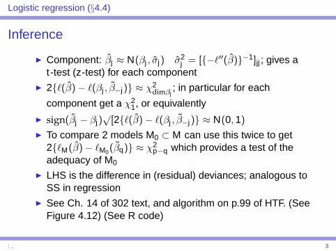
Inference
I Component: β̂j ≈ N(βj , σ̂j) σ̂2j = [{−`′′(β̂)}−1]jj ; gives a
t-test (z-test) for each componentI 2{`(β̂)− `(βj , β̃−j)} ≈ χ2
dimβj; in particular for each
component get a χ21, or equivalently
I sign(β̂j − βj)√
[2{`(β̂)− `(βj , β̃−j)} ≈ N(0, 1)
I To compare 2 models M0 ⊂ M can use this twice to get2{`M(β̂)− `M0
(β̃q)} ≈ χ2p−q which provides a test of the
adequacy of M0
I LHS is the difference in (residual) deviances; analogous toSS in regression
I See Ch. 14 of 302 text, and algorithm on p.99 of HTF. (SeeFigure 4.12) (See R code)
: , 3
Logistic regression (§4.4)
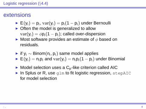
extensionsI E(yi) = pi , var(yi) = pi(1− pi) under BernoulliI Often the model is generalized to allow
var(yi) = φpi(1− pi); called over-dispersionI Most software provides an estimate of φ based on
residuals.
I if yi ∼ Binom(ni , pi) same model appliesI E(yi) = nipi and var(yi) = nipi(1− pi) under Binomial
I Model selection uses a Cp-like criterion called AICI In Splus or R, use glm to fit logistic regression, stepAIC
for model selection
: , 4
Logistic regression (§4.4)
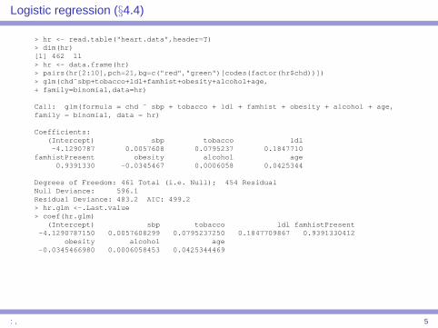
> hr <- read.table("heart.data",header=T)> dim(hr)[1] 462 11> hr <- data.frame(hr)> pairs(hr[2:10],pch=21,bg=c("red","green")[codes(factor(hr$chd))])> glm(chd˜sbp+tobacco+ldl+famhist+obesity+alcohol+age,+ family=binomial,data=hr)
Call: glm(formula = chd ˜ sbp + tobacco + ldl + famhist + obesity + alcohol + age,family = binomial, data = hr)
Coefficients:(Intercept) sbp tobacco ldl
-4.1290787 0.0057608 0.0795237 0.1847710famhistPresent obesity alcohol age
0.9391330 -0.0345467 0.0006058 0.0425344
Degrees of Freedom: 461 Total (i.e. Null); 454 ResidualNull Deviance: 596.1Residual Deviance: 483.2 AIC: 499.2> hr.glm <-.Last.value> coef(hr.glm)
(Intercept) sbp tobacco ldl famhistPresent-4.1290787150 0.0057608299 0.0795237250 0.1847709867 0.9391330412
obesity alcohol age-0.0345466980 0.0006058453 0.0425344469
: , 5
Logistic regression (§4.4)
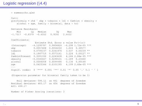
> summary(hr.glm)
Call:glm(formula = chd ˜ sbp + tobacco + ldl + famhist + obesity +
alcohol + age, family = binomial, data = hr)
Deviance Residuals:Min 1Q Median 3Q Max
-1.7517 -0.8379 -0.4552 0.9292 2.4432
Coefficients:Estimate Std. Error z value Pr(>|z|)
(Intercept) -4.1290787 0.9606826 -4.298 1.72e-05 ***sbp 0.0057608 0.0056250 1.024 0.30577tobacco 0.0795237 0.0261876 3.037 0.00239 **ldl 0.1847710 0.0573161 3.224 0.00127 **famhistPresent 0.9391330 0.2243638 4.186 2.84e-05 ***obesity -0.0345467 0.0290531 -1.189 0.23440alcohol 0.0006058 0.0044490 0.136 0.89168age 0.0425344 0.0101295 4.199 2.68e-05 ***---Signif. codes: 0 ‘***’ 0.001 ‘**’ 0.01 ‘*’ 0.05 ‘.’ 0.1 ‘ ’ 1
(Dispersion parameter for binomial family taken to be 1)
Null deviance: 596.11 on 461 degrees of freedomResidual deviance: 483.17 on 454 degrees of freedomAIC: 499.17
Number of Fisher Scoring iterations: 3
: , 6
Logistic regression (§4.4)
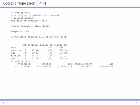
> library(MASS)> hr.step <- stepAIC(hr.glm,trace=F)> anova(hr.step)Analysis of Deviance Table
Model: binomial, link: logit
Response: chd
Terms added sequentially (first to last)
Df Deviance Resid. Df Resid. DevNULL 461 596.11tobacco 1 41.46 460 554.65ldl 1 23.13 459 531.52famhist 1 24.28 458 507.24age 1 21.80 457 485.44> coef(hr.step)
(Intercept) tobacco ldl famhistPresent age-4.20381991 0.08069792 0.16757435 0.92406001 0.04403574
: , 7
Logistic regression (§4.4)
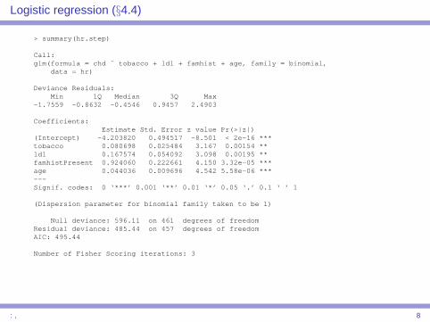
> summary(hr.step)
Call:glm(formula = chd ˜ tobacco + ldl + famhist + age, family = binomial,
data = hr)
Deviance Residuals:Min 1Q Median 3Q Max
-1.7559 -0.8632 -0.4546 0.9457 2.4903
Coefficients:Estimate Std. Error z value Pr(>|z|)
(Intercept) -4.203820 0.494517 -8.501 < 2e-16 ***tobacco 0.080698 0.025484 3.167 0.00154 **ldl 0.167574 0.054092 3.098 0.00195 **famhistPresent 0.924060 0.222661 4.150 3.32e-05 ***age 0.044036 0.009696 4.542 5.58e-06 ***---Signif. codes: 0 ‘***’ 0.001 ‘**’ 0.01 ‘*’ 0.05 ‘.’ 0.1 ‘ ’ 1
(Dispersion parameter for binomial family taken to be 1)
Null deviance: 596.11 on 461 degrees of freedomResidual deviance: 485.44 on 457 degrees of freedomAIC: 495.44
Number of Fisher Scoring iterations: 3
: , 8
Logistic regression (§4.4)
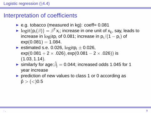
Interpretation of coefficientsI e.g. tobacco (measured in kg): coeff= 0.081I logit{pi(β)} = βT xi ; increase in one unit of xij , say, leads to
increase in logitpi of 0.081; increase in pi/(1− pi) ofexp(0.081) = 1.084.
I estimated s.e. 0.026, logitpi ± 0.026,exp(0.081 + 2× .026), exp(0.081− 2× .026)) is(1.03, 1.14).
I similarly for age:β̂j = 0.044; increased odds 1.045 for 1year increase
I prediction of new values to class 1 or 0 according asp̂ > (<)0.5
: , 9
Logistic regression (§4.4)
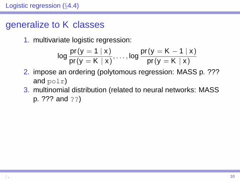
generalize to K classes
1. multivariate logistic regression:
logpr(y = 1 | x)
pr(y = K | x), . . . , log
pr(y = K − 1 | x)
pr(y = K | x)
2. impose an ordering (polytomous regression: MASS p. ???and polr )
3. multinomial distribution (related to neural networks: MASSp. ??? and ??)
: , 10
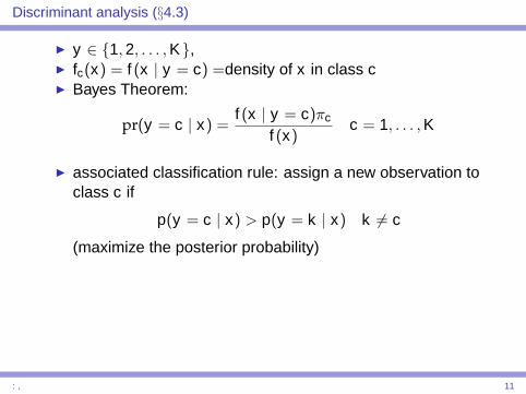
Discriminant analysis (§4.3)
I y ∈ {1, 2, . . . , K},I fc(x) = f (x | y = c) =density of x in class cI Bayes Theorem:
pr(y = c | x) =f (x | y = c)πc
f (x)c = 1, . . . , K
I associated classification rule: assign a new observation toclass c if
p(y = c | x) > p(y = k | x) k 6= c
(maximize the posterior probability)
: , 11
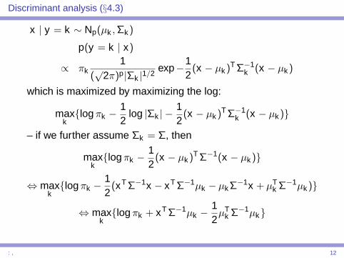
Discriminant analysis (§4.3)
x | y = k ∼ Np(µk ,Σk )
p(y = k | x)
∝ πk1
(√
2π)p|Σk |1/2exp−1
2(x − µk )T Σ−1
k (x − µk )
which is maximized by maximizing the log:
maxk{log πk −
12
log |Σk | −12(x − µk )T Σ−1
k (x − µk )}
– if we further assume Σk = Σ, then
maxk{log πk −
12(x − µk )T Σ−1(x − µk )}
⇔ maxk{log πk −
12(xT Σ−1x − xT Σ−1µk − µkΣ−1x + µT
k Σ−1µk )}
⇔ maxk{log πk + xT Σ−1µk −
12µT
k Σ−1µk}
: , 12
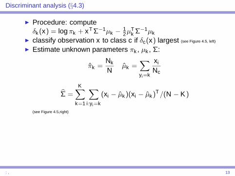
Discriminant analysis (§4.3)
I Procedure: computeδk (x) = log πk + xT Σ−1µk − 1
2µTk Σ−1µk
I classify observation x to class c if δc(x) largest (see Figure 4.5, left)
I Estimate unknown parameters πk , µk , Σ:
π̂k =Nk
Nµ̂k =
∑yi=k
xi
Nc
Σ̂ =K∑
k=1
∑i:yi=k
(xi − µ̂k )(xi − µ̂k )T /(N − K )
(see Figure 4.5,right)
: , 13
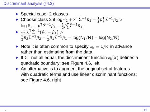
Discriminant analysis (§4.3)
I Special case: 2 classesI Choose class 2 if log π̂2 + xT Σ̂−1µ̂2 − 1
2 µ̂T2 Σ̂−1µ̂2 >
log π̂1 + xT Σ̂−1µ̂1 − 12 µ̂T
1 Σ̂−1µ̂1,I ⇔ xT Σ̂−1(µ̂2 − µ̂1) >
12 µ̂2Σ̂
−1µ̂2 − 12 µ̂1Σ̂
−1µ̂1 + log(N1/N)− log(N2/N)
I Note it is often common to specify πk = 1/K in advancerather than estimating from the data
I If Σk not all equal, the discriminant function δk (x) defines aquadratic boundary; see Figure 4.6, left
I An alternative is to augment the original set of featureswith quadratic terms and use linear discriminant functions;see Figure 4.6, right
: , 14
Discriminant analysis (§4.3)
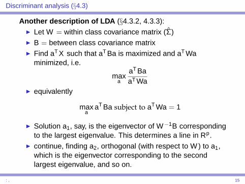
Another description of LDA (§4.3.2, 4.3.3):I Let W = within class covariance matrix (Σ̂)I B = between class covariance matrixI Find aT X such that aT Ba is maximized and aT Wa
minimized, i.e.
maxa
aT BaaT Wa
I equivalently
maxa
aT Ba subject to aT Wa = 1
I Solution a1, say, is the eigenvector of W−1B correspondingto the largest eigenvalue. This determines a line in Rp.
I continue, finding a2, orthogonal (with respect to W ) to a1,which is the eigenvector corresponding to the secondlargest eigenvalue, and so on.
: , 15
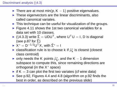
Discriminant analysis (§4.3)
I There are at most min(p, K − 1) positive eigenvalues.I These eigenvectors are the linear discriminants, also
called canonical variates.I This technique can be useful for visualization of the groups.I Figure 4.11 shows the 1st two canonical variables for a
data set with 10 classes.I (§4.3.3) write Σ̂ = UDUT , where UT U = I, D is diagonal
(see p.87 for Σ̂)I X ∗ = D−1/2UT X , with Σ̂∗ = II classification rule is to choose k if µ̂∗k is closest (closest
class centroid)I only needs the K points µ̂∗k , and the K − 1 dimension
subspace to compute this, since remaining directions areorthogonal (in the X ∗ space)
I if K = 3 can plot the first two variates (cf wine data)I See p.92, Figures 4.4 and 4.8 (algorithm on p.92 finds the
best in order, as described on the previous slide): , 16
Discriminant analysis (§4.3)
NotesI §4.2 considers linear regression of 0, 1 variable on several
inputs (odd from a statistical point of view)I how to choose between logistic regression and
discriminant analysis?I they give the same classification error on the heart data (is
this a coincidence?)I logistic regression and generalizations to K classes
doesn’t assume any distribution for the inputsI discriminant analysis more efficient if the assumed
distribution is correctI warning: in §4.3 x and xi are p × 1 vectors, and we
estimate β0 and β, the latter a p × 1 vectorI in §4.4 they are (p + 1)× 1 with first element equal to 1
and β is (p + 1)× 1.
: , 17
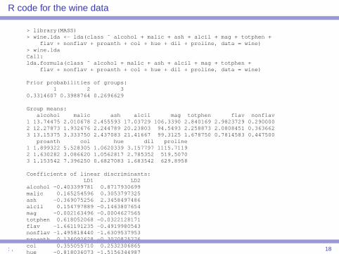
R code for the wine data
> library(MASS)> wine.lda <- lda(class ˜ alcohol + malic + ash + alcil + mag + totphen +
flav + nonflav + proanth + col + hue + dil + proline, data = wine)> wine.ldaCall:lda.formula(class ˜ alcohol + malic + ash + alcil + mag + totphen +
flav + nonflav + proanth + col + hue + dil + proline, data = wine)
Prior probabilities of groups:1 2 3
0.3314607 0.3988764 0.2696629
Group means:alcohol malic ash alcil mag totphen flav nonflav
1 13.74475 2.010678 2.455593 17.03729 106.3390 2.840169 2.9823729 0.2900002 12.27873 1.932676 2.244789 20.23803 94.5493 2.258873 2.0808451 0.3636623 13.15375 3.333750 2.437083 21.41667 99.3125 1.678750 0.7814583 0.447500
proanth col hue dil proline1 1.899322 5.528305 1.0620339 3.157797 1115.71192 1.630282 3.086620 1.0562817 2.785352 519.50703 1.153542 7.396250 0.6827083 1.683542 629.8958
Coefficients of linear discriminants:LD1 LD2
alcohol -0.403399781 0.8717930699malic 0.165254596 0.3053797325ash -0.369075256 2.3458497486alcil 0.154797889 -0.1463807654mag -0.002163496 -0.0004627565totphen 0.618052068 -0.0322128171flav -1.661191235 -0.4919980543nonflav -1.495818440 -1.6309537953proanth 0.134092628 -0.3070875776col 0.355055710 0.2532306865hue -0.818036073 -1.5156344987dil -1.157559376 0.0511839665proline -0.002691206 0.0028529846
Proportion of trace:LD1 LD2
0.6875 0.3125> plot(wine.lda)
: , 18
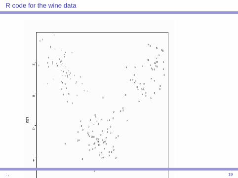
R code for the wine data
-6 -4 -2 0 2 4-6
-4-2
02
LD1LD2
1
1
1
1
1
111
1
1
1 111
1
11
1
1
1
1
11
1
11
1
11
1 1
1
1
11
1
1
1
1
1
1
1
1
1
1
1
1
1
1
1
1
11
1
1
1
1
11
2
2 2
2
2
2
2
22
2
2
2
2
2
2
2
2
2
2
2
2
2
2
2
2
2
2
22
2
2
2 2
2
2 2
2
2
2
2
2
2
2
2
2
2
2
2
2
2
2
2
2
2
2
2
2
22
2
2
2
2
2
2
2
2
2
2
2
2
3
3
3
3
3
3
3
3
3
3
3
3
33
3
3
3
33
33 3
3
3
3
3
3
3
3
3
3
3
3
3
3
3
3
33
3
3
3
33
3
3
3
3
: , 19
Separating hyperplanes (§4.5)
I assume two classes only; change notation so that y = ±1I use linear combinations of inputs to predict y
y =
{−1+1
asβ0 + xT β < 0β0 + xT β > 0
I misclassification error D(β, β0) = −Σi∈Myi(β0 + xTi β)
whereI M = {j ; yj(β0 + xT
j β) < 0}I note that D(β) > 0 and proportional to the ’size’ of β0 +xT
i β
I Can show that an algorithm to minimize D(β, β0) exists andconverges the the plane that separates y = +1 fromy = −1 if such a plane exists
I But it will cycle if no such plane exists and be very slow ifthe ’gap’ is small
: , 20
Separating hyperplanes (§4.5)
I Also if one plane exists there is likely many (Figure 4.13)I The plane that defines the ”largest” gap is defined to be
”best”I can show that this needs to
minβ0,β
12||β||2
s.t. yi(β0 + xTi β) ≥ 1, i = 1, . . . N (4.44)
I See Figure 4.15I the points on the edges (margin) of the gap called support
points or support vectors; there are typically many fewer ofthese than original points
I this is the basis for the development of Support VectorMachines (SVM), more later
I sometimes add features by using basis expansions; to bediscussed first in the context of regression (Chapter 5)
: , 21