Embed Size (px)
Citation preview

Research Division Federal Reserve Bank of St. Louis Working Paper Series
Frictionless Technology Diffusion: The Case of Tractors
Rodolfo E. Manuelli
and Ananth Seshadri
Working Paper 2013-022B
http://research.stlouisfed.org/wp/2013/2013-022.pdf
February 2013 Revised July 2013
FEDERAL RESERVE BANK OF ST. LOUIS Research Division
P.O. Box 442 St. Louis, MO 63166
______________________________________________________________________________________
The views expressed are those of the individual authors and do not necessarily reflect official positions of the Federal Reserve Bank of St. Louis, the Federal Reserve System, or the Board of Governors.
Federal Reserve Bank of St. Louis Working Papers are preliminary materials circulated to stimulate discussion and critical comment. References in publications to Federal Reserve Bank of St. Louis Working Papers (other than an acknowledgment that the writer has had access to unpublished material) should be cleared with the author or authors.

Frictionless Technology Diffusion: The Case of
Tractors
Rodolfo E. Manuelli
Washington University in St. Louis
and Federal Reserve Bank of St. Louis
Ananth Seshadri ∗
University of Wisconsin-Madison
July 9, 2013
Abstract
Many new technologies display long adoption lags, and this is often interpreted as
evidence of frictions inconsistent with the standard neoclassical model. In this paper
we study the diffusion of the tractor in American agriculture between 1910 and 1960
– a well known case of slow diffusion – and show that the speed of adoption was
consistent with the predictions of a simple neoclassical growth model. The reason
for the slow rate was that tractor quality kept improving over this period and, more
importantly, that only when wages increased did it become relatively unprofitable to
operate the alternative, labor-intensive, horse technology.

I. Introduction
Understanding the determinants of the rate at which new technologies are created and
adopted is a critical element in the analysis of growth. Even though modeling equilibrium
technology creation can be somewhat challenging for standard economic theory, understand-
ing technology adoption should not be. Specifically, once the technology is available, the
adoption decision is equivalent to picking a point on the appropriate isoquant. Dynamic con-
siderations make this calculation more complicated, but they still leave it in the realm of
the neoclassical model. A simple minded application of the theory of the firm suggests that
profitable innovations should be adopted instantaneously, or with some delay depending on
various forms of cost of adjustment.
The evidence on the adoption of new technologies seems to contradict this prediction.
Jovanovic and Lach (1997) report that, for a group of 21 innovations, it takes 15 years for
its diffusion to go from 10% to 90%, the 10-90 lag. They also cite the results of a study
by Grübler (1991) covering 265 innovations who finds that, for most diffusion processes, the
10-90 lag is between 15 and 30 years.1
In response to this apparent failure of the simple neoclassical model, a large number
of papers have introduced ‘frictions’ to account for the ‘slow’adoption rate. These fric-
tions include, among others, learning-by-doing (e.g. Jovanovic and Lach (1989), Jovanovic
and Nyarko (1996), Greenwood and Yorukoglu (1997), Felli and Ortalo-Magné (1997), and
Atkeson and Kehoe (2001)), vintage human capital (e.g. Chari and Hopenhayn (1994) and
Greenwood and Yorukoglu (1997)), informational barriers and spillovers across firms (e.g.
Jovanovic and Macdonald (1994)), resistance on the part of sectoral interests (e.g. Parente
and Prescott (1994)), coordination problems (e.g. Shleifer (1986)), search-type frictions (e.g.
Manuelli (2002)) and indivisibilities (e.g. Greenwood, Seshadri and Yorukoglu (2004)).
In this paper we take a step back and revisit the implications of the neoclassical fric-
tionless model for the equilibrium rate of diffusion of a new technology. Our model has
two features that influence the rate at which a new technology is adopted: changes in the
1

price of inputs other than the new technology and changes in the quality of the technology.2
The application that we consider throughout is another famous case of ‘slow’adoption: the
farm tractor in American agriculture. The tractor was a very important innovation that
dramatically changed the way farming was carried out and had a very large impact on farm
productivity, making this a study worthwhile in its own right. In addition, there is a large
literature on the diffusion of the tractor technology and the common finding in this literature
is that diffusion was too slow.3
We assume a standard neoclassical technology that displays constant returns to scale
in all factors. In order to eliminate frictions associated with indivisible inputs, we study
the case in which there are perfect rental markets for all inputs.4 The representative farm
operator maximizes profits choosing the mix of inputs. Given our market structure, this is
a static problem. We take prices and the quality of all inputs as exogenous and we let the
model determine the price of one input, land, so as to guarantee that demand equals the
available stock.
We use a mixture of calibration and estimation to pin down the relevant parameters. We
then use the model, driven by the observed changes in prices, wages and real interest rates to
predict the number the tractors and employment for the entire 1910-1960 period. The model
is very successful in explaining the diffusion of the tractor – including the S-shape diffusion
curve– and does reasonably well in tracing the demise of the horse. Even though it was not
designed for this purpose, it does a very good job in capturing the change in employment
over the same time period. In addition, the implications for land prices are in line with
the available evidence. We conclude that there is no tension between the predictions of a
frictionless neoclassical model and the rate at which tractors diffused in U.S. agriculture.
More generally, our findings show that stable S-shape diffusion curves need not be
structural objects. Rather, their shape need not reflect the “frictions” that we described
above, and may simply be the outcome of standard profit maximization when the model is
correctly specified. In particular, we find that ignoring changes in the quality of a technology
2
over time and in the costs of operating alternative (often less productive) technologies can
account for the pattern of diffusion.
The paper is organized as follows. In section 2 we present a brief historical account of
the diffusion of the tractor and of the price and quality variables that are the driving forces
in our model. Section 3 describes the model, and Section 4 discusses the determination of
the relevant parameters. Sections 5 and 6 present our results, and section 7 offers some
concluding comments.
II. Some Historical Observations
This section presents some evidence the use of tractors and horses by U.S. farmers, and
on the behavior of wages and employment in the U.S. agricultural sector.
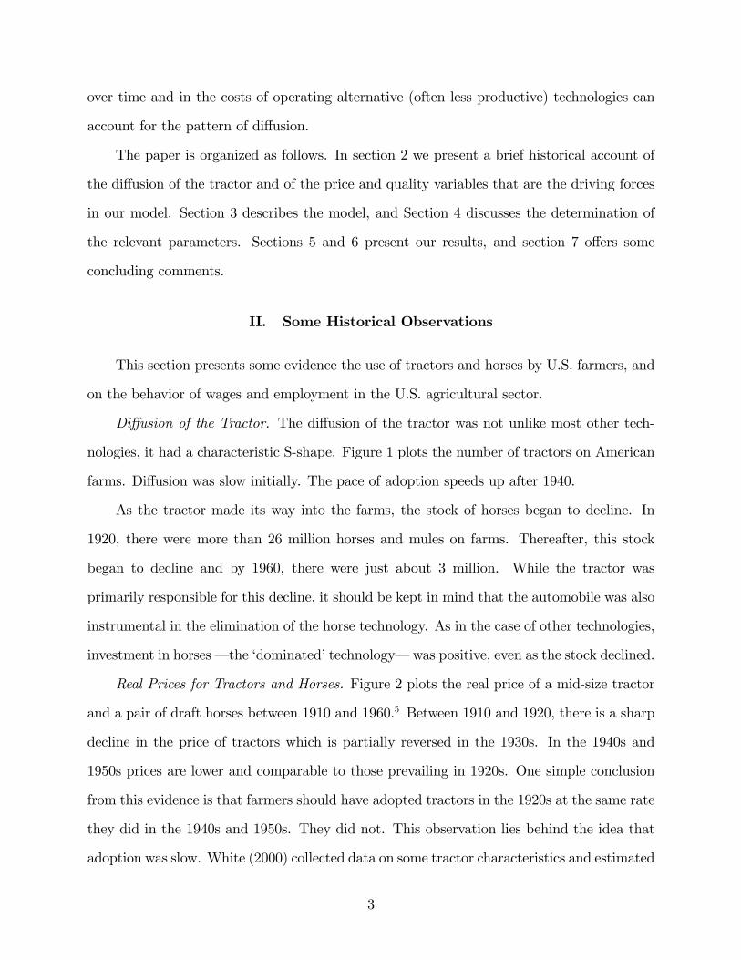
Diffusion of the Tractor. The diffusion of the tractor was not unlike most other tech-
nologies, it had a characteristic S-shape. Figure 1 plots the number of tractors on American
farms. Diffusion was slow initially. The pace of adoption speeds up after 1940.
As the tractor made its way into the farms, the stock of horses began to decline. In
1920, there were more than 26 million horses and mules on farms. Thereafter, this stock
began to decline and by 1960, there were just about 3 million. While the tractor was
primarily responsible for this decline, it should be kept in mind that the automobile was also
instrumental in the elimination of the horse technology. As in the case of other technologies,
investment in horses – the ‘dominated’technology– was positive, even as the stock declined.
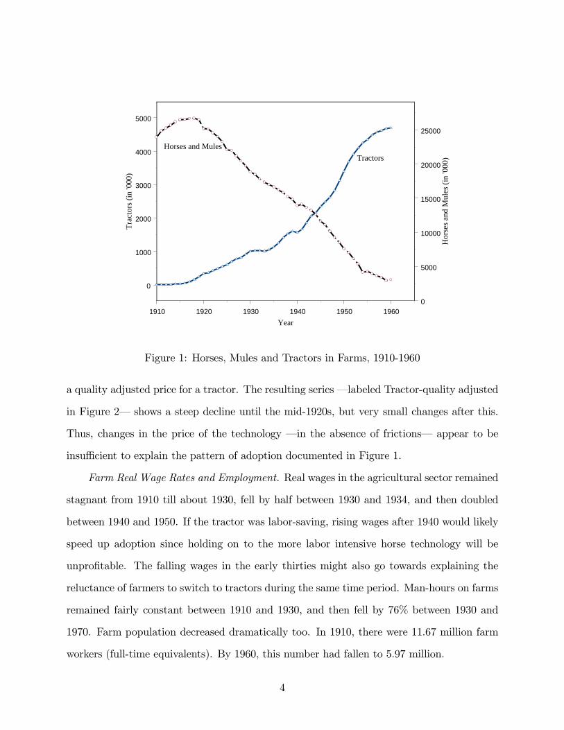
Real Prices for Tractors and Horses. Figure 2 plots the real price of a mid-size tractor
and a pair of draft horses between 1910 and 1960.5 Between 1910 and 1920, there is a sharp
decline in the price of tractors which is partially reversed in the 1930s. In the 1940s and
1950s prices are lower and comparable to those prevailing in 1920s. One simple conclusion
from this evidence is that farmers should have adopted tractors in the 1920s at the same rate
they did in the 1940s and 1950s. They did not. This observation lies behind the idea that
adoption was slow. White (2000) collected data on some tractor characteristics and estimated
3
1910 1920 1930 1940 1950 1960Year
0
1000
2000
3000
4000
5000Tr
acto
rs (i
n '0
00)
0
5000
10000
15000
20000
25000
Hor
ses a
nd M
ules
(in
'000
)
Horses and MulesTractors
Figure 1: Horses, Mules and Tractors in Farms, 1910-1960
a quality adjusted price for a tractor. The resulting series – labeled Tractor-quality adjusted
in Figure 2– shows a steep decline until the mid-1920s, but very small changes after this.
Thus, changes in the price of the technology – in the absence of frictions– appear to be
insuffi cient to explain the pattern of adoption documented in Figure 1.
Farm Real Wage Rates and Employment. Real wages in the agricultural sector remained
stagnant from 1910 till about 1930, fell by half between 1930 and 1934, and then doubled
between 1940 and 1950. If the tractor was labor-saving, rising wages after 1940 would likely
speed up adoption since holding on to the more labor intensive horse technology will be
unprofitable. The falling wages in the early thirties might also go towards explaining the
reluctance of farmers to switch to tractors during the same time period. Man-hours on farms
remained fairly constant between 1910 and 1930, and then fell by 76% between 1930 and
1970. Farm population decreased dramatically too. In 1910, there were 11.67 million farm
workers (full-time equivalents). By 1960, this number had fallen to 5.97 million.
4

1910 1920 1930 1940 1950 1960Year
0
20
40
60
80
100
120R
eal P
rice
of H
orse
s and
Tra
ctor
s
Horse
Tractor quality adjusted
Tractor
0.2
0.7
1.2
1.7
2.2
2.7
Rea
l Wag
e R
ate
Wage
Figure 2: Real Prices for Tractors, Horses and Labor: 1910-1960
In what follows we develop a simple neoclassical growth model of agricultural production
and investment and show that the previous evidence is consistent with optimal frictionless
adoption of tractors once the change in the effective price of operating the tractor technology
– which depends on changes in quality and price of tractors as well as wage rates– relative
to the cost of operating the more labor intensive horse technology are explicitly taken into
account. In our setting, “slow” adoption is neither evidence of deviations from perfect
markets, indivisibilities, or other “frictions.”
Alternative Explanations. The standard approach to studying the diffusion of the tractor
is based on the ‘threshold’model. In its simplest form, the model takes as given the size
of the farm (in acres) and considers the costs of different combinations of horse-drawn and
tractor-drawn technologies required to produce a given amount of services. By choosing the
cost minimizing technology, the model selects the type (size) of farm that should adopt a
tractor. The predictions of the model – given the size distribution of farms – are then
5

compared with the data. These calculations find that in the 1920’s and early 1930’s, U.S.
farmers were too slow to adopt the relatively new tractor technology. Allowing for imperfect
capital markets (Clarke (1991)) or introducing uncertainty about the value of output (Lew
(2001)) help improve the fit of the model, but not to the point where it is consistent with
the evidence. More recently Olmstead and Rhode (2001) estimate that changes in the price
of horses and in the size distribution delayed, to some extent, the adoption of tractors. In
their model the size distribution is exogenous. White (2000) emphasizes the role of prices
and quality of tractors. Using a hedonic regression, he computes a quality-adjusted price
series for tractors. White conjectures that the increase in tractor quality should be taken
into account to understand adoption decisions.
III. A Simple Model of Farming
Our approach is to model technology adoption using a standard profit maximization
argument. Since we assume complete rental markets, the maximization problem is static.6
The one period profit of a farmer is given by,
πt(qt, ct, wt) ≡ maxkt,ht,nt,at
pctF (kt, ht, nt, at)−t∑
τ=−∞[qkt(τ) + ckt(τ)]mkt(τ)− [qht + cht]ht − wtn̄t − [qat + cat]at,
where F (kt, ht, nt, at) is a standard production function which we assume to be homogeneous
of degree one in all inputs, and kt is the demand for tractor services, ht is the demand for
horse services (which we assume proportional to the stock of horses), nt = (nht, nkt, nyt)
is a vector of labor services corresponding to three potential uses: operating horses, nht,
operating tractors, nkt, or other farm tasks, nyt, and at is the demand for land services
(which we assume proportional to acreage), and n̄t = nht + nkt + nyt is the total demand for
labor.
On the cost side, qht + cht is the full cost of operating a draft of horses. The term
6
qht is the rental price of a horse, and cht includes operating costs (e.g. feed and veterinary
services). The term qat + cat is the full cost of using one acre of land, and wt is the cost of
one unit of (farm) labor. Effective one period rental prices for horses and land (two durable
goods) are given by
qjt ≡ pjt −(1− δjt)pjt+1
1 + rt+1, j = h, a,
where δjt are the relevant depreciation factors, and rt is the interest rate.
Since we view changes in the quality of tractors as a major factor influencing the decision
to adopt the technology, we specified the model so that it could capture such variations.
Specifically, we assume that tractor services can be provided by tractors of different vintages,
τ , according to
kt =t∑
τ=−∞mkt(τ)k̃t(τ),
where k̃t(τ) is the quantity of tractor services provided by a tractor of vintage τ (i.e. built
in period τ) at time t, and mkt(τ) is the number of tractors of vintage τ operated at time t.
We assume that the amount of tractor services provided at time t by a tractor of vintage τ
is given by,
k̃t(τ) ≡ v(xτ )(1− δkτ )t−τ ,
where δkτ is the depreciation rate of a vintage τ tractor, and v(xτ ) maps model-specific
characteristics, the vector xτ , into an overall index of tractor ‘services’or ‘quality.’ Thus,
our model assumes that the characteristics of a tractor are fixed over its lifetime (i.e. no
upgrades), and that tractors depreciate at a rate that is (possibly) vintage specific. The
rental price of a tractor is given by
qkt(τ) = pkt(τ)− pkt+1(τ)
1 + rt+1,
where pkt(τ) is the price at time t of a t− τ year old tractor, while the term ckt(τ) captures
the variable cost (fuel, repairs) associated with operating one tractor of vintage τ at time t.
7
The resulting demand for input functions for is denoted by
mt = m(qt, ct, wFt ),
where m ∈ {k, h, a, n̄} indicates the input type, qt is a vector of rental prices, ct is a vector
of operating costs, and wFt denotes real wages in the farm sector. Given that agricultural
prices are largely set in world markets, and that domestic and total demand do not coincide,
we impose as an equilibrium condition that the demand for land equal the available supply.
Thus, land prices are endogenously determined.
A. Aggregate Implications
Aggregation in this model is standard. However, it is useful to make explicit the con-
nection between the demand for tractor services and the demand for tractors.
The aggregate demand for tractor services at time t, Kt is given by
(1) Kt = k(qt, ct, wt),
while the number of tractors purchased at t, mkt is
(2) mkt =Kt − (1− δkt−1)Kt−1
v(xt).
The law of motion for the stock of tractors (in units), Kt, is7
(3) Kt = (1− δkt−1)Kt−1 +mkt.
It follows that to compute the implications of the model for the stock of tractors, which
is the variable that we observe, it is necessary to determine the depreciation factors and the
quality of tractors of each vintage.
We assume that horse services are proportional to the stock of horses and, by choice of
8

a constant, we set the proportionality ratio to one. Thus, the aggregate demand for horses
is
(4) Ht = h(qt, ct, wt).
We let the price of land adjust so that the demand for land predicted by the model
equals the total supply of agricultural land denoted by At. Thus, given wages, agricultural
prices and horse and tractor prices, the price of land, pat, adjusts so that
(5) At = a(qt, ct, wt).
B. Modeling Tractor Prices
From the point of view of an individual farmer the relevant price of tractor is qkt(τ) : the
price of tractor services corresponding to a t− τ year old tractor in period t. Unfortunately,
data on these prices are not available. However, given a model of tractor price formation, it is
possible to determine rental prices for all vintages using standard, no-arbitrage, arguments.
As indicated above, we assume that a new tractor at time t offers tractor services given
by k̃t(t) = v(xt), where v(xt) is a function that maps the characteristics of a tractor into
tractor services. We assume that, at time t, the price of a new tractor is given by
pkt =v(xt)
γct.
In this setting γ−1ct is a measure of markup over the level of quality. If the industry is
competitive, it is interpreted as the amount of aggregate consumption required to produce
one unit of tractor services using the best available technology xt.8 However, if there is
imperfect competition, it is a mixture of the cost per unit of quality and a standard markup.
For the purposes of understanding tractor adoption we need not distinguish between these
two interpretations: any factor – technological change or variation in markups– that affects
9

the cost of tractors will have an impact on the demand for them. In what follows we ignore
this distinction, and we label γct as productivity in the tractor industry.
No arbitrage arguments imply that
(6) qkt(t) = pkt
[1−Rt(1)(1− δkt)
γctγct+1
]+ (1−∆t)C(t+ 1, T − 1),
where
∆t =v(xt)(1− δkt)
v(xt+1),
C(t+ 1, T − 1) ≡T−1∑j=0
Rt+1(j)ckt+1+j,
Rt(j) ≡j∏
k=1
(1 + rt+k)−1
given that T is the lifetime of a tractor, and ckt is the cost of operating a tractor in period t.
This expression has a simple interpretation. The first term, 1 − Rt(1)(1 − δkt)γctγct+1
,
translates the price of a tractor into its flow equivalent. If there were no changes in the
unit cost of tractor quality, i.e. γct = γct+1, this term is just that standard capital cost,
(rt+1 + δkt)/(1 + rt+1). The second term is the flow equivalent of the present discounted
value of the costs of operating a tractor from t to t + T − 1, C(t + 1, T − 1). In this case,
the adjustment factor, 1 −∆t, includes more than just depreciation: total costs have to be
corrected by the change in the ‘quality’of tractors, which is captured by the ratio v(xt)v(xt+1)
.
Equation 6 illustrates the forces at work in determining the rental price of a tractor:
• Increases in the price of a new tractor, pkt(t), increase the cost of operating it. This is
the (standard) price effect.
• Periods of anticipated productivity increases – low values of γctγct+1
– result in increases
in the rental price of tractors. This effect is the complete markets analog of the option
value of waiting: buyers of a tractor at t know that, due to decreases in the price of
10

new tractors in the future, the value of their used unit will be lower. In order to get
compensated for this, they require a higher rental price.
• The term (1 − ∆t+1)C(t + 1, T − 1) captures the increase in cost per unit of tractor
services associated with operating a one year old tractor, relative to a new tractor.
IV. Model Specification, Calibration and Estimation
We begin by describing how we estimate the rental price of tractor services. To compute
qkt(t) we need to separately identify v(xt) and γct.9 To this end we specified that the price
of a tractor of model m, produced by manufacturer k at time t, pmkt, is given by
pmkt = e−dtΠNj=1(x
mjt)
λjeεmt ,
where xmt = (xm1t, xm2t, ...x
mNt) is a vector of characteristics of a particular model produced at
time t, the dt variables are time dummies, and εmt is a shock. This formulation is consistent
with the findings of White (2000).10 We used data on prices, tractor sales and a large
number of characteristics for almost all models of tractors produced between 1919 and 1955 to
estimate this equation. In the Appendix, we describe the data and the estimation procedure.
Given our estimates of the time dummy, d̂t, and the price of each tractor, p̂mkt, we computed
our estimate of average quality, v̄(xt) as
v̄(xt) = p̄ktγ̂ct,
where
p̄kt =∑m
smktp̂mkt,
γ̂ct = ed̂t ,
11

Figure 3: Tractor Prices, Quality and Productivity. 1920-1955. Estimation Results.
with smkt being the share of model m produced by manufacturer k in total sales at time t.
The resulting time-series for v̄(xt), γ̂ct and p̄kt are shown in Figure 3.
Even though the real price of the average tractor does not show much of trend after
1920, its components do. Over the whole period our index of quality more than doubles,
and our measure of productivity shows a substantial, but temporary, increase in the 1940s
relative to trend, only to return to trend in the 1950s. In the 1920-1955 period γct increases
by about 50%. Thus, during this period there were substantial increases in quality and
decreases in costs; however, these two factors compensated each other (except at the very
end), so that the real price of a tractor shows a modest increase.
We assume that the interest rate is time varying and that R = (1 + r)−1. We consider
12
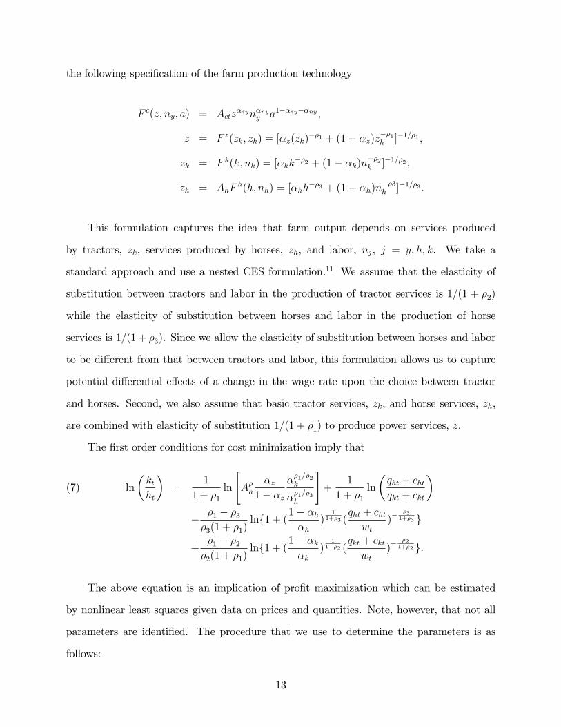
the following specification of the farm production technology
F c(z, ny, a) = Actzαzynαnyy a1−αzy−αny ,
z = F z(zk, zh) = [αz(zk)−ρ1 + (1− αz)z−ρ1h ]−1/ρ1 ,
zk = F k(k, nk) = [αkk−ρ2 + (1− αk)n−ρ2k ]−1/ρ2 ,
zh = AhFh(h, nh) = [αhh
−ρ3 + (1− αh)n−ρ3h ]−1/ρ3 .
This formulation captures the idea that farm output depends on services produced
by tractors, zk, services produced by horses, zh, and labor, nj, j = y, h, k. We take a
standard approach and use a nested CES formulation.11 We assume that the elasticity of
substitution between tractors and labor in the production of tractor services is 1/(1 + ρ2)
while the elasticity of substitution between horses and labor in the production of horse
services is 1/(1 + ρ3). Since we allow the elasticity of substitution between horses and labor
to be different from that between tractors and labor, this formulation allows us to capture
potential differential effects of a change in the wage rate upon the choice between tractor
and horses. Second, we also assume that basic tractor services, zk, and horse services, zh,
are combined with elasticity of substitution 1/(1 + ρ1) to produce power services, z.
The first order conditions for cost minimization imply that
ln
(ktht
)=
1
1 + ρ1ln
[Aρh
αz1− αz
αρ1/ρ2k
αρ1/ρ3h
]+
1
1 + ρ1ln
(qht + chtqkt + ckt
)(7)
− ρ1 − ρ3ρ3(1 + ρ1)
ln{1 + (1− αhαh
)1
1+ρ3 (qht + chtwt
)− ρ31+ρ3 }
+ρ1 − ρ2ρ2(1 + ρ1)
ln{1 + (1− αkαk
)1
1+ρ2 (qkt + cktwt
)− ρ21+ρ2 }.
The above equation is an implication of profit maximization which can be estimated
by nonlinear least squares given data on prices and quantities. Note, however, that not all
parameters are identified. The procedure that we use to determine the parameters is as
follows:
13

1. Given values of (αzy, αny, αz, αk, αh), we estimate equation (7). This allows us to
recover value of the parameters that determine the elasticities of substitution ρ1, ρ2, ρ3)
as well an estimate of Ah.
2. Given those estimates, and using the series for full prices of the two technologies –
(qkt + ckt) and (qht + cht)– we obtain the unit costs of zk and zh, the services of the
two technologies.
3. With estimates of unit costs and given the level of gross farm output, F c, we determine
the quantity of each factor (k, h, ny, nk, nh) used in the production of farm output from
the profit maximization conditions. We adjust TFP so that the model’s predictions
for output match what is observed in the data each year.
4. Next, we compute the implications of the model for:
(a) Land share in agriculture.
(b) The (stock) of horses relative to output in 1910 and 1960.
(c) The (stock) of tractors relative to output in 1910 and 1960.12
5. Finally, we iterate by choosing different values of (αzy, αny, αz, αk, αh), and reestimat-
ing the model in each round, until the predictions of the model match the data.
The results of the NLLS estimation of equation (7) with a Gaussian error term added
to it are given in Table 1.13 The dependent Variable is ln(ktht
): the ratio of tractor services
to horse services which is a variable that we constructed according to the model described
in the previous section.
We take the process {Act} to correspond to total factor productivity. Even though there
are estimates of the evolution of TFP for the agricultural sector, it is by no means obvious
how to use them. The problem is that, conditional on the model, part of measured TFP
changes is due to changes in the quality of tractors, v(xt), as well as the rate of diffusion
14

Variable Estimate t-statisticρ1 -0.8167 -8.26ρ2 -0.4068 -2.88ρ3 -0.100 -2.31
R2(adj) 0.920
Table 1: NLLS Estimation
of tractors. Thus, in our model, conventionally measured TFP is endogenous. To compute
(truly) exogenous TFP we used the following identification assumption: TFP is adjusted so
that the model’s prediction for the change in output between 1910 and 1960 match the data.
This gives us an estimate of γ,the growth rate of TFP, which corresponds to an end-to-end
change by a factor of 1.6. By way of comparison, the Historical Statistics reports that overall
farm TFP grew by a factor of 2.3.
Table 2 presents the match between the model and U.S. data for our chosen specification
- the five moments are used for calibration purposes. The match is good in terms of all of
the aggregate moments.
1910 1960Moment Model Data Model Data SourceLand - share of output 0.2 0.2 Binswanger and Ruttan (1978)Horses/output ratio 0.25 0.25 0.009 0.01 Hist.Stat.of U.S.Tractors/output ratio 0.0031 0.0031 0.135 0.135 Hist.Stat.of U.S.
Table 2: Match Between Model and Data, 1910 & 1960
The parameters that we use are in Table 3.14
Parameter Ah αzy αny αz αk αhValue 0.75 0.38 0.42 0.56 0.54 0.41
Table 3: Calibration
The estimated values for ρ1, ρ2 and ρ3 deserve some discussion. The estimate of the de-
gree of substitutability between the two services, ρ1 is 5.46. This implies that tractor services
and horse services are very good substitutes. Furthermore, the degree of substitutability be-
tween tractors and labor (1.7) is greater than the degree of substitutability between horses
15

7.9
8.4
8.9
9.4
9.9
10.4
0
1
2
3
4
5
6
7
8
9
1910 1915 1920 1925 1930 1935 1940 1945 1950 1955 1960Year
Tractors Model
Tractors Data
Horses DataHorses Model
Figure 4: Transitional Dynamics, 1910-1960 - Tractors and Horses
and labor (1.1). This differential substitution effect plays an important role when the wage
rate changes.15
V. Was Diffusion Too Slow?
The results for 1960 indicate that the model does a reasonable job of matching some of
the key features of the data. However, they are silent about the model’s ability to account
for the speed at which the tractor was adopted.
Was diffusion too slow? To answer this question, the entire dynamic path from 1910 to
1960 needs to be computed. To do this, we took the observed path for prices (pk, ph, pc, w, r),
operating costs (ck, ch, ca) and depreciation rates (δk, δh, δa), and use them as inputs to
compute the predictions of the model for the 1910-1960 period.16 At the same time, we
adjusted the time path of TFP so that the model matches the data in terms of the time
path of agricultural output, the analog of our steady state procedure. This helps to get
the scale right along the entire transition. Thus, the model matches agricultural output by
construction.
16
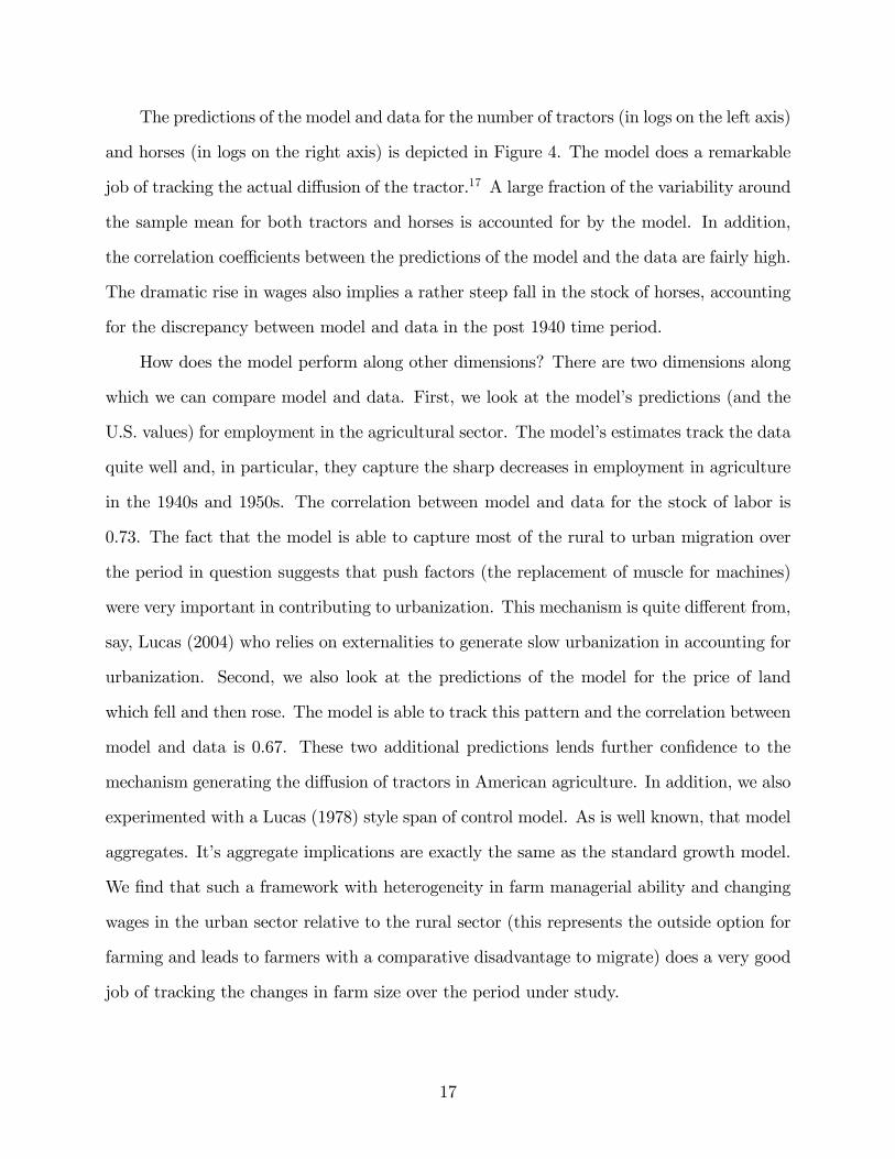
The predictions of the model and data for the number of tractors (in logs on the left axis)
and horses (in logs on the right axis) is depicted in Figure 4. The model does a remarkable
job of tracking the actual diffusion of the tractor.17 A large fraction of the variability around
the sample mean for both tractors and horses is accounted for by the model. In addition,
the correlation coeffi cients between the predictions of the model and the data are fairly high.
The dramatic rise in wages also implies a rather steep fall in the stock of horses, accounting
for the discrepancy between model and data in the post 1940 time period.
How does the model perform along other dimensions? There are two dimensions along
which we can compare model and data. First, we look at the model’s predictions (and the
U.S. values) for employment in the agricultural sector. The model’s estimates track the data
quite well and, in particular, they capture the sharp decreases in employment in agriculture
in the 1940s and 1950s. The correlation between model and data for the stock of labor is
0.73. The fact that the model is able to capture most of the rural to urban migration over
the period in question suggests that push factors (the replacement of muscle for machines)
were very important in contributing to urbanization. This mechanism is quite different from,
say, Lucas (2004) who relies on externalities to generate slow urbanization in accounting for
urbanization. Second, we also look at the predictions of the model for the price of land
which fell and then rose. The model is able to track this pattern and the correlation between
model and data is 0.67. These two additional predictions lends further confidence to the
mechanism generating the diffusion of tractors in American agriculture. In addition, we also
experimented with a Lucas (1978) style span of control model. As is well known, that model
aggregates. It’s aggregate implications are exactly the same as the standard growth model.
We find that such a framework with heterogeneity in farm managerial ability and changing
wages in the urban sector relative to the rural sector (this represents the outside option for
farming and leads to farmers with a comparative disadvantage to migrate) does a very good
job of tracking the changes in farm size over the period under study.
17
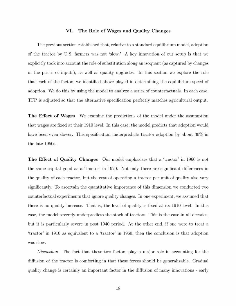
VI. The Role of Wages and Quality Changes
The previous section established that, relative to a standard equilibriummodel, adoption
of the tractor by U.S. farmers was not ‘slow.’ A key innovation of our setup is that we
explicitly took into account the role of substitution along an isoquant (as captured by changes
in the prices of inputs), as well as quality upgrades. In this section we explore the role
that each of the factors we identified above played in determining the equilibrium speed of
adoption. We do this by using the model to analyze a series of counterfactuals. In each case,
TFP is adjusted so that the alternative specification perfectly matches agricultural output.
The Effect of Wages We examine the predictions of the model under the assumption
that wages are fixed at their 1910 level. In this case, the model predicts that adoption would
have been even slower. This specification underpredicts tractor adoption by about 30% in
the late 1950s.
The Effect of Quality Changes Our model emphasizes that a ‘tractor’in 1960 is not
the same capital good as a ‘tractor’ in 1920. Not only there are significant differences in
the quality of each tractor, but the cost of operating a tractor per unit of quality also vary
significantly. To ascertain the quantitative importance of this dimension we conducted two
counterfactual experiments that ignore quality changes. In one experiment, we assumed that
there is no quality increase. That is, the level of quality is fixed at its 1910 level. In this
case, the model severely underpredicts the stock of tractors. This is the case in all decades,
but it is particularly severe in post 1940 period. At the other end, if one were to treat a
‘tractor’in 1910 as equivalent to a ‘tractor’in 1960, then the conclusion is that adoption
was slow.
Discussion: The fact that these two factors play a major role in accounting for the
diffusion of the tractor is comforting in that these forces should be generalizable. Gradual
quality change is certainly an important factor in the diffusion of many innovations - early
18

incarnations of the new technology are pretty crude and slowly evolve with time.18 While
quality change has been considered before, they have not been modeled in the gradual fashion
in which we model it. The close tie up between the our estimation and our model simulation
is a feature worth emphasizing. Furthermore, most other work (see, for instance, Greenwood
and Yorukoglu, 1997) model the evolution of quality as a one shot event, moving up to the
frontier right away - even though they assume a gradual decline in the price of capital. Our
results make it very clear that such a consideration would lead the researcher to conclude,
rather incorrectly, that diffusion was slow!
One of the key mechanisms identified in the prevailing literature on technology diffusion
is that if old capital and new capital are complementary inputs, the marginal product of
investment depends not only on the vintage of technology but also on the amount of old
capital available for that specific vintage. Even when new technologies are available, people
invest in old technologies if there exist abundant old capital for these technologies. As a
consequence, diffusion of new technologies is slow. This is the mechanism at work in both
Chari and Hopenhayn (1991) and many subsequent papers. Indeed in Chari and Hopenhayn
(1991) ρ1 = −1; in this case, only one of the two technologies will be in use and the gradual
diffusion will be inconsistent with the standard model. The mechanisms at work in our model
generate a slower pattern of adoption if the services obtained from the two technologies are
(imperfect) substitutes. Imperfect substitutability of the two technologies plays a crucial
role in understanding the diffusion of the tractor.
VII. The Role of Other Factors
We explored the sensitivity of the results to changes in a number of other factors. For
brevity, we do not report the detailed results. Our analysis describes the effects of other
‘counterfactuals’holding the path of TFP constant.
19

The Role of Horse Prices Recent research on the topic of adoption of tractors has
emphasized that adjustment of horse prices delayed the diffusion of tractors (see Olmstead
and Rhode (2001)). In the context of this model, fixing horse prices at their 1910 levels has
hardly any effect on adoption. The reason is simple: horse prices are a relatively unimportant
component of the cost of operating the horse technology. Should we conclude that explicitly
modeling the fact that farmers had a choice between an ‘old’ and a ‘new’ technology is
an unnecessary feature of the model? No. The reason is simple: given that the horse
technology is labor intensive, we would have missed a channel through which wage changes
induce changes in the degree of mechanization.
Elasticity of Substitution Our specification of the technology is such that, at our pre-
ferred parameterization, the elasticity of substitution between tractor and horse services is
rather high. In order to quantitatively assess the importance of this specification, we studied
a version of the model in which ρ1 = ρ2 = ρ3 = 0. In this case, the model severely under-
predicts the diffusion of the tractor. The reason for this result is simple: the Cobb-Douglas
functional form implies constant input shares. In the absence of spectacular price decreases
in the own price – and tractor prices showed a large, but not spectacular decrease over this
period – the model predicts modest increases in the quantities demanded.
Finally, one can ask whether the level of generality in the nested CES added value. We
conducted a series of experiments and our conclusion is that the degree of substitutability
between tractor and horse services is the most important one. Indeed, if we set ρ1 = ρ2 and
set ρ3 = 0, the equation governing the k/h ratio becomes linear and the fit of the equation
is nearly as good as the NLLS presented above. This experiment suggests that the key to
our results is allowing for the two types of services to be substitutable. Restricting the horse
services technology to be Cobb-Douglas and assuming that the degree of substitutability
between the two types of services to be the same as that between capital and labor in the
production of tractor services does little violence to the predictions of the model.
20

VIII. Conclusions
The frictionless neoclassical framework has been used to study a wide variety of phe-
nomena including growth and development.19 However, the perception that the observed
rate at which many new technologies have been adopted is too slow to be consistent with the
model, has led to the development of alternative frameworks which include some ‘frictions.’
In this paper we argue that a careful modeling of the shocks faced by an industry suggests
that the neoclassical model can be consistent with ‘slow’adoption.20 Since most models
with ‘frictions’are such that the equilibrium is not optimal, the choice between standard
convex models and the various alternatives has important policy implications. It is clearly
an open question how far our results can be generalized. By this, we mean the idea that to
understand the speed at which a technology diffuses it is necessary to carefully model both
the cost of operating alternative technologies and the evolution of quality. We point to some
examples that suggest that the forces that we emphasize play a role more generally.
Consider first, the diffusion of nuclear power plants. While the technology to harness
electricity from atoms was clearly available in the 1950s, diffusion of Nuclear power plants
was rather ‘slow’. Rapid diffusion did not take place until 1971. In 1971, Nuclear’s share
of total electricity generation was less than 4%. This number shot up to 11% by 1980 and
around 20% by 1990 and remained at that level. What was the impetus for such a change?
The obvious factor was the oil shock of the 1970s which dramatically increased the real
price of crude oil and induced a substitution away from the use of fossil fuels to uranium.
Furthermore, when the price of oil came down, the United States stopped building nuclear
reactors. The other factor that played an important role in putting a stop to the diffusion of
nuclear power plants is the high operating cost associated with waste disposal. Nuclear power
plants have generated 35000 tons of radioactive waste, most of which is stored at the plants
in special pools or canisters. But the plants are running out of room and until a permanent
storage facility is opened up, the diffusion of nuclear power plants will proceed slowly. All
this suggests that changes in the price of substitutes (oil) and changes in operating costs can
21

go a long way toward accounting for the diffusion of nuclear power plants.
A second example is the case of diesel-electric locomotives. The first diesel locomotive
was built in the U.S. in 1924, but the technology did not diffuse until the 1940s and 1950s.
It seems that the key factor in this case was a substantial improvement in quality: increased
fuel effi ciency relative to its steam counterpart and possibly more important, reduced labor
requirements. Since, as we documented in the paper, wages rose substantially during World
War II, quality improvements reduced the cost of operating the diesel technology relative to
the steam technology.
Our theory is rather simple - perhaps the simplest possible theory wherein the evolution
of relative prices can account for slow adoption. There is nothing inherent in the Neoclassical
theory that suggests that adoption will be slow. However, not all historical episodes suggest
slow adoption. One example is the rather rapid adoption of ATM machines replacing bank
tellers in India. Our preliminary analysis of that case study indicates that changes in the
prices of ATMs relative to wages can account for a very large fraction of diffusion.
Of course, a few examples, no matter how persuasive they appear, cannot ‘prove’that
factors that are usually ignored in the macro literature on adoption are important. However,
at the very least, they cast a doubt on the necessity of ‘frictions’in accounting for the rate
of diffusion of new technologies.
22

REFERENCES
Acemoglu, Daron and Fabrizio Zilibotti, ‘Productivity Differences,’Quarterly Journal of
Economics, Vol. 115, No. 3 (2001): 563-606.
Atkeson, Andrew and Patrick Kehoe, ‘The Transition to a New Economy After the Second
Industrial Revolution,’NBER Working Paper No.W8676, Dec. 2001.
Becker, Gary S, Human Capital: A Theoretical and Empirical Analysis, with Special Refer-
ence to Education, University of Chicago Press, 1964.
Bils, Mark and Pete Klenow, ‘Quantifying Quality Growth,’American Economic Review 91
(September 2001): 1006-1030.
Binswanger, H., and V. W. Ruttan. 1978. Induced Innovation: Technology, Institutions and
Development. Baltimore: Johns Hopkins University Press.
Chari, V.V. and H. Hopenhayn, ‘Vintage Human Capital, Growth and the Diffusion of New
Technology’Journal of Political Economy,Vol. 99, No. 6. (Dec. 1991): 1142-1165.
Clarke, Sally, ‘New Deal Regulation and the Revolution in American Farm Productivity:
A Case Study of the Diffusion of the Tractor in the Corn Belt, 1920-1940,’The Journal of
Economic History, Vol. 51, No. 1. (Mar., 1991): 101-123.
Cole, Harold and Lee Ohanian, ‘New Deal Policies and the Persistence of the Great Depres-
sion: A General Equilibrium Analysis,’Journal of Political Economy, forthcoming.
Dunning, Lorry, The Ultimate American Farm Tractor Data Book : Nebraska Test Tractors
1920-1960 (Farm Tractor Data Books), 1999.
Ortalo-Magné, François and Leonardo Felli “Technological Innovations: Slumps and Booms,”
with , Centre for Economic Performance, Paper No. 394, London School of Economics, 1998.
23

Greenwood, Jeremy, “The Third Industrial Revolution: Technology, Productivity and In-
come Inequality," AEI Studies on Understanding Economic Inequality, Washington, DC:
The AEI Press, 1997.
Greenwood, Jeremy, Ananth Seshadri and Mehmet Yorukoglu, ‘Engines of Liberation,’Re-
view of Economic Studies, forthcoming.
Greenwood, Jeremy and Mehmet Yorukoglu, “1974,”Carnegie-Rochester Series on Public
Policy, 46, (June 1997): 49-95.
Griliches, Zvi. ‘Hybrid Corn: An Exploration of the Economics of Technological Change.’In
Technology, Education and Productivity: Early Papers with Notes to Subsequent Literature.
pp. 27-52 (New York, Basil Blackwell, 1957).
Jovanovic, Boyan and Glenn M. MacDonald, “Competitive Diffusion,”Journal of Political
Economy, Vol. 102, No. 1. (Feb., 1994): 24-52.
Jovanovic, Boyan and Yaw Nyarko, “Learning by Doing and the Choice of Technology,”
Econometrica, Vol. 64, No. 6. (Nov., 1996): 1299-1310.
Jovanovic, Boyan and Saul Lach, “Entry, Exit, and Diffusion with Learning by Doing,”
American Economic Review, Vol. 79, No. 4. (Sep., 1989): 690-99.
Jovanovic, Boyan and Saul Lach, “Product Innovation and the Business Cycle,”International
Economic Review, Vol. 38, Issue 1. (Feb., 1997): 3-22.
Kislev, Yoav and Willis Peterson, ‘Prices, Technology, and Farm Size,’Journal of Political
Economy, Vol. 90, No. 3. (Jun. 1982): 578-595.
Lew, Byron, ‘The Diffusion of Tractors on the Canadian Prairies: The Threshold Model and
the Problem of Uncertainty,’Explorations in Economic History 37, (2000): 189—216.
Lucas, Robert E. Jr., ‘On the Size Distribution of Business Firms,’Bell Journal of Economics
9, no.2 (Autumn 1978): 508-23.
24
Lucas, Robert E. Jr., ‘Life Earnings and Rural-Urban Migration,’The Journal of Political
Economy, Vol. 112, No. 1 (Feb. 2004): S29-S59.
Manuelli, Rodolfo, ‘Technological Change, the Labor Market, and the Stock Market,’mimeo,
University of Wisconsin-Madison, 2002.
Olmstead, Alan L., and Paul W. Rhode, "Reshaping the Landscape: The Impact and Diffu-
sion of the Tractor in American Agriculture, 1910—1960," Journal of Economic History, 61
(Sept. 2001), 663—98.
Oster, Sharon, “The Diffusion of Innovation Among Steel Firms: The Basic Oxygen Fur-
nace,”The Bell Journal of Economics, Volume 13, Issue 1, (Spring, 1982): 45-56.
Parente, Stephen L. and Edward C. Prescott. “Barriers to Technology Adoption and Devel-
opment,”Journal of Political Economy, Vol., 102, No. 2 (Apr. 1994): 298-321.
Rose, Nancy L and Paul L. Joskow, “The Diffusion of New Technologies: Evidence from
the Electric Utility Industry,”The RAND Journal of Economics, Vol. 21, Issue 3 (Autumn,
1990): 354-373.
Shleifer, A. (1986), “Implementation Cycles”, Journal of Political Economy, Vol. 94, 1163—
1190.
Whatley, Warren C., “A History of Mechanization in the Cotton South: The Institutional
Hypothesis,”The Quarterly Journal of Economics, Vol. 100, No. 4, (Nov. 1985), pp: 1191-
1215.
White, William J. III, ‘An Unsung Hero: The Farm Tractor’s Contribution to Twentieth-
Century United States Economic Growth,’unpublished dissertation, The Ohio State Uni-
versity, 2000.
USDA. 1936 Agricultural Statistics. Washington, DC: GPO, 1936.
25

USDA. 1942 Agricultural Statistics. Washington, DC: GPO, 1942.
USDA. 1949 Agricultural Statistics. Washington, DC: GPO, 1949.
USDA. 1960 Agricultural Statistics. Washington, DC: GPO, 1961.
USDA. Income Parity for Agriculture, Part III. Prices Paid by Farmers for Commodities
and Services, Section 4, Prices Paid by Farmers for Farm Machinery and Motor Vehicles,
1910-38. Prel. Washington DC, (May 1939).
USDA. Income Parity for Agriculture, Part II: Expenses for Agricultural Production, Section
3: Purchases, Depreciation, and Value of Farm Automobiles, Motortrucks, Tractors and
Other Farm Machinery. Washington, DC: GPO, 1940.
U.S. Bureau of the Census. Historical Statistics of the United States: Millennial Edition
Online. http://hsus.cambridge.org
26

IX. Appendix
A. Data Sources
This section details the available data, the sources which they were obtained and what
they were used for. The data were used to calibrate the model and to compare the model
and the data.
Income and Output
Value of Gross Farm Output : HS Series Da1271 - used for computing factor shares and for
calibration.
Land
Land in Farms: HS Series Da566-used to compute the prices of land over time and to
compare model and data.
Land Prices
Lindert, Peter H. (1998), "Long-run Trends in American Farmland Values," Working
Paper, UC-Davis
Labor
Farm Employment : HS Series Da612 - used to compute Labor’s share of income and to
compare model and data.
Wage Rates: Data provided by Heady used to compute labor’s share of farm income and as
an exogenous driving process
Capital - Tractors and Horses
Number of Tractors on farms: HS Series Da623 - used to compute tractor’s share of farm
income
Number of Horses and Mules on farms: HS Series Da991 and Da992 - used to compute
horses’s share of farm income
Depreciation Rates and Operating Costs for Tractors: For the period 1910-1940, we used
data from USDA. Income Parity for Agriculture, Part II. For the period 1941-1960, we used
27
data from USDA, Agricultural Statistics - used as exogenous driving processes
Horse Prices: Data provided by Paul Rhode - used to compute horses’s share of farm income
and as an exogenous driving process
Tractor Prices: From 1920 to 1955, we used data from on our hedonic estimations. These
estimations were based upon data on tractor prices and characteristics kindly provided to us
by WilliamWhite and augmented to include additional characteristics from Dunning (2000).
For the period 1910-1919, and 1956-1960, we extrapolated the data using our estimation and
data on average price of tractor available from the USDA, Agricultural Statistics. The exact
manner in which this was done is described in the Appendix. This series is used to compute
tractor’s share of farm income and as an exogenous driving process.
B. Derivation of the User Cost of a Tractor
From
pkt(t) =v(xt)
γct,
and given that a vintage-τ tractor at time t provides tractor services equal to k̃t(τ) ≡
v(xτ )(1− δkτ )t−τ , the rental price of such a tractor at time t is
qkt(τ) = pkt(τ)− pkt+1(τ)
1 + rt+1.
This simply says that a t−τ year old tractor at time t will be a t−τ +1 year old tractor
at t+ 1. This formula has the drawback that it depends on the price of used tractors. Since
there are no data available on used tractor prices we now proceed to derive an expression for
qkt(τ) using simple arbitrage arguments. One can show that the optimal choice of mkt(τ)
requires that
pctFk(t)k̃t(τ) = pkt(τ)− pkt+1(τ)
1 + rt+1+ ckt(τ).
Iterating forward and denoting by T (τ , t) the number of periods of useful life that a
28

t− τ old tractor has left, we get that
pkt(τ) =
T (τ ,t)∑j=0
Rt(j){pct+jFk(t+ j)k̃t+j(τ)− ckt+j(τ)},
where Rt(j) is as defined in the text. Using the special structure of kt(τ) it follows that
pkt+1(τ) = γkτv(xτ )(1−δkτ )t+1−τT (τ ,t+1)∑j=0
Rt+1(j)pct+1+jFk(t+1+j)(1−δkτ )j−T (τ ,t+1)∑j=0
Rt+1(j)ckt+1+j(τ).
Let the present discounted value of the cost of operating a tractor for T − 1 periods starting
at t+ 1 be given by
C(t+ 1, T − 1) ≡T−1∑j=0
Rt+1(j)ckt+1+j.
Let T (τ , t) be the remaining lifetime at time t of a tractor of time τ vintage. Then, it follows
that
pkt+1(t) =v(xt)(1− δkt)
v(xt+1)pkt+1(t+ 1)−
[1− v(xt)(1− δkt)
v(xt+1)
] T (t,t+1)∑j=0
Rt+1(j)ckt+1+j
+v(xt)(1− δkt)
v(xt+1){T (t,t+1)∑j=0
Rt+1(j)pct+1+jFk(t+ 1 + j)(1− δkt)j(1− (1 + ϕ)j)
−T (t+1,t+1)∑j=T (t,t+1)
Rt+1(j)[pct+1+jFk(t+ 1 + j)(1− δkt+1)j − ckt+1+j]},
where
δkt+1 = δkt − ϕ(1− δkt).
To simplify the presentation we assume that two consecutive vintages of tractors have
the same depreciation and economic lifetime (ϕ = 0 and T (t + 1, t + 1) = T (t, t + 1) + 1).
Moreover, we assume that operating costs vary over time, but are not a function of the
vintage, i.e. ckt+j(τ) = ckt+j, for all τ . In this case, using the previous formula for τ = t
29

(one period old tractors) and τ = t+ 1 (new tractors) it follows that
pkt+1(t) =v(xt)(1− δkt)
v(xt+1)pkt+1(t+ 1)−
[1− v(xt)(1− δkt)
v(xt+1)
] T−1∑j=0
Rt+1(j)ckt+1+j(t)
+v(xt)(1− δkt)
v(xt+1)Rt+1(T )
[pct+1+TFk(t+ 1 + T )v(xt+1)(1− δkt)T − ckt+1+T
].
However, the last term in square brackets must be zero, since a tractor of vintage
t + 1 is optimally scrapped when the marginal product of its remaining tractor services,
pct+1+TFk(t+ 1 + T )v(xt+1)(1− δkt)T , equals the marginal cost of operating it, ckt+1+T .
Let the present discounted value of the cost of operating a tractor for T − 1 periods
starting at t+ 1 be given by
C(t+ 1, T − 1) ≡T−1∑j=0
Rt+1(j)ckt+1+j,
and the ‘effective’depreciation of a vintage t tractor between t and t+1 be∆t+1 ≡ v(xt)(1−δkt)v(xt+1)
.
It follows that,
qkt(t) = pkt(t)
[1−Rt(1)(1− δkt)
γctγct+1
]+ (1−∆t+1)C(t+ 1, T − 1)
which is the expression (6) in the text.
C. Estimation of Tractor Prices
In order to compute the user cost of tractor services, we need to estimate the effect that
different factors have upon tractor prices. Our basic specification is
ln pmkt = −dt +
N∑j=0
λj lnxmjt + εmt,
30

where pmkt is the price of a model m tractor produced by manufacturer m at time t, the
vector xmt = (xm1t, xm2t, ...x
mNt) is a vector of characteristics of a particular model produced at
time t, the dt variables are time dummies, and εmt is a shock that we take to be independent
of the xmjt variables and independent across models and years. We estimated the previous
equation by OLS using a sample of 1345 tractor-year pairs covering the period 1920-1955.
The basic data comes from two sources. William White very generously shared with us
the data he collected which includes prices, sales volume and several technical variables. A
description of the sample can be found in his dissertation, White (2000). We complemented
White’s sample with additional technical information obtained from the Nebraska Tractor
Tests covering the 1920-1960 period, as reported by Dunning (1999). The variables in the x
vector included technical specifications as well as manufacturer dummies. In the following
table we present the point estimates of the technical variables.21
Variable Estimate t Variable Estimate tFuelCost 0.129 5.19 Row Crop (D) -0.031 -2.56Cylinders 0.047 0.93 High Clear (D) -0.026 -0.98Gears 0.103 3.58 Rubber Tires (D) 0.162 5.17RPM -0.170 -3.26 Tractor Fuel (D) -0.164 -2.82HP 0.627 21.89 Kerosene-Gasoline (D) 0.028 1.27Plow Speed 0.067 1.33 Distillate-Gasoline (D) -0.029 -1.74Slippage -0.030 -2.38 All Fuel (D) -0.041 -1.70Length -0.127 -2.36 Diesel-Gasoline (D) -0.042 -1.65Weight 0.163 5.24 Diesel (D) 0.006 0.09Speed -0.081 -2.38 LPG (D) -0.207 -1.95
Table 4: Regression Results. Point Estimates and t-statistics. A (D) denotes a dummyvariable.
In addition, we included 15 manufacturer dummies and 35 time dummies. We selected
the variables we used from a larger set, from which we eliminated one of a pair whenever the
simple correlation coeffi cient between two variables exceeded 0.80. We experimented using
a smaller set of variables as in White (2000), but our estimates of the time dummies were
practically identical.22
Our data covers the period 1920-1955. However, the period we are interested in studying
31
is 1910-1960. Thus, we need to extend the average price and the time dummies to cover the
missing years. The price data for 1910-1919 come from Olmstead and Rhode (2001), and
it corresponds to the price of a ‘medium tractor’. For the period 1956-1960 we used the
price of an average tractor as published by the USDA. Inspection of the pattern of the time
dummies – the line labeled Gamma in Figure 3– suggest a fairly non-linear trend. If we
exclude the war-time years, it seems as if productivity was relatively constant since the mid
1930s. Thus, for the 1956-1960 period we assume that there was no change in γct. The
situation is quite different from 1910 to 1920, as this is a period of rapidly falling prices. We
estimated the time dummies for the period 1910-1919 from a regression of the time dummies
over the 1920-1935 period (before they ‘stabilize’) on time and time square. Our estimated
values imply that most of the drop in tractor prices in this period is due to increases in
productivity (more than 80%). This is consistent with the accounts that important changes
in the tractor technology did not occurred until the 1920s.
32