Frictional Wage Dispersion in Search Models:

A Quantitative Assessment

Andreas Hornstein∗ Per Krusell† Giovanni L. Violante‡

August 10, 2010

Abstract

In a large class of search models, we derive a tight prediction for a measureof frictional wage dispersion—the mean-min wage ratio—that depends on statis-tics of labor-market turnover (unemployment inflow and outflow rates, job-to-jobtransitions) and preference parameters (discount rate, value of non-market time),but is independent of the wage-offer distribution. For plausible parameterizationsof preferences, the observed magnitude of worker flows implies that in the basicsearch model, and in most of its extensions, frictional wage dispersion is very small.Notable exceptions are some of the most recent models of on-the-job search, wheresizeable frictional wage dispersion can coexist with observed labor-market transi-tions. Because of its broad applicability, our new metric allows us to rationalize thediverse empirical findings in the large literature estimating structural labor-marketmodels with frictions. Our findings are also relevant for business-cycle studies, asthey reveal that search models face a trade-off between frictional wage dispersionin the cross-section and cyclical unemployment fluctuations in the time-series.

∗Federal Reserve Bank of Richmond†IIES Stockholm University, CEPR, and NBER‡New York University, CEPR and NBER

1 Introduction

Does the law of one price hold in the labor market, i.e., are identical workers paid the

same wage? We use the term frictional wage dispersion for any departures from the law

of one price, and the goal in this paper is to assess its quantitative magnitude. Since the

labor market is the main source of income for most individuals, the amount of frictional

wage inequality should be informative for anyone interested in efficiency, equity, and the

provision of social insurance.1

Our approach is to use observed worker choice, along with search theory (as in McCall,

1970, Mortensen, 1970, and countless follow-up studies), to infer the frictional component

of wage dispersion. The specific observations that we exploit are worker flow data from

the labor market (such as unemployment duration and separation rates). Moreover, we

place quantitative restrictions on the preference parameters that appear in our search

models (discount rates and the value of non-market time).

A central methodological finding in our paper is that for the wide range of search

models we consider, one can derive a measure of frictional wage dispersion without any

knowledge of the wage-offer distribution the worker is drawing from. This measure is

the “mean-min wage ratio”, i.e., the ratio of the average accepted wage to the lowest

accepted, or reservation, wage. It turns out that the mean-min ratio in all these search

models can be related, in simple closed form, to the preference parameters and the flow

statistics; in the very most basic search model, for example, the mean-min ratio is an easily

interpretable function of the discount rate, the value of non-market time, the separation

rate, and the unemployment duration. This tight relation between the mean-min ratio and

a small set of model parameters is merely an implication of optimal job search behavior,

and it is independent of the particular equilibrium mechanism underlying the wage-offer

distribution.

Thus, we argue that it is a misconception to think that search models can generate

any amount of wage differentials as long as the wage-offer distribution is sufficiently dis-

persed, because there is a causal link—dictated by optimal job search behavior—between

the wage-offer dispersion and worker flows, on which there is reliable survey data. Put

differently, for given preference parameters, the amount of frictional wage dispersion in

search models is constrained by the observed size of the transition rates of workers.

When calibrating the baseline search model, for plausible values of preference param-

eters, the observed labor-market transition rates imply a mean-min ratio of 1.05, i.e., the

1A similar view is expressed in Mortensen (2005, page 2).

1

average wage can only be five percent above the lowest wage paid. Through the lenses

of this particular class of search models, deviations from the law of one price are thus

minor. The key reason for this finding is the short duration of unemployment spells in

the data. Intuitively, given that unemployed workers choose to take jobs quickly, they

must not perceive a high option value of waiting for better job offers. In the basic model,

this option value is determined precisely by wage dispersion. Taking workers’ flow data at

face value, one can escape the conclusion of a very low mean-min ratio only if workers are

implausibly impatient or have an implausibly low (indeed negative) value of non-market

time.

We use search models, together with worker flow data, to quantify the extent of fric-

tional wage dispersion because direct empirical estimates are fraught with measurement

problems. Ideally, a direct estimate of frictional wage dispersion requires the empirical

distribution of wages for identical workers employed in the same narrowly defined labor

market. In practice though, it is very difficult, if not impossible, to obtain such reliable

data. Individual surveys offer very limited information on worker and job characteristics;

e.g., differences across workers in their skills, preferences, and outside opportunities and

across jobs in their amenities are inherently challenging to appraise and thus make it

hard to isolate wage dispersion due to frictions alone. The most common measures are

estimates of “residual” wage dispersion from a Mincerian wage regression with as many

control variables as possible. These regressions typically imply 50-10 wage percentile ra-

tios between 1.7 and 1.9 for male workers in the recent years (Acemoglu, 2002, Figure 3;

Lemieux, 2006, Figure 1A; Autor, Katz and Kearney, 2008, Figure 8). Given the skew-

ness of the wage distribution and the fact that the 10th percentile is above the lowest

wage paid, the 50-10 ratio is a conservative estimate of the mean-min ratio. Because of

the omitted variables in the regression, these wage ratios based on residual inequality

represent upper bounds for actual frictional wage dispersion.2

In the second part of the paper, we ask what type of changes in the basic model would

allow greater frictional wage dispersion to coexist with empirical observations on worker

flows. The basic search model relies on four assumptions that we relax one by one: (i)

perfect correlation between job values and initial wage; (ii) risk neutrality; (iii) random

search; and (iv) no on-the-job search. For all of these extensions, we can derive closed-form

expressions for the mean-min ratio that are easy to interpret and evaluate quantitatively.

The generality of our analysis builds on the fact that a solution for the mean-min ratio

2In Hornstein et al. (2007a), we use a variety of data sources and methodologies to control forunobserved heterogeneity and measurement error. We arrive at estimates of residual wage dispersionwhich imply mean-min ratios between 1.5 and 2.

2

always arises very naturally from the reservation wage equation, the cornerstone of optimal

job search.

The first three extensions—where we allow for imperfect correlation between job value

and wages, for risk aversion, and for directed search—do not lead to anything but very

minor adjustments of the benchmark mean-min ratio. Thus, our basic quantitative finding

that frictional wage dispersion is small holds in a wider range of search models.

The fourth extension, allowing on-the-job search, has much richer implications. In-

tuitively, if workers can also search while employed, they may optimally choose to exit

quickly from unemployment even in presence of a very dispersed distribution of wage of-

fers, since they do not completely give up the option value of search. The mean-min wage

ratio derived from Burdett’s (1978) job ladder model shows that the higher the arrival

rate of offers on the job, the larger is frictional wage dispersion in the model. Therefore,

in models of on-the-job search, it is the frequency of job-to-job transitions, besides unem-

ployment duration, that constrains the magnitude of frictional wage dispersion. Under the

same calibration for preferences as in the baseline model, now the observed labor-market

flows can coexist with wage dispersion up to five times as large, i.e., the mean-min wage

ratio is around 1.25. Therefore, through the lenses of models with on-the-job search, de-

viations from the law of one price are more significant, albeit still fairly minor in absolute

size.

We continue our study of models with on-the-job search by considering environments

where search effort is endogenous (Christensen et al., 2005), and where employers have the

ability to make counteroffers (Postel-Vinay and Robin, 2002a, 2002b; Dey and Flinn, 2005;

Cahuc, Postel-Vinay and Robin, 2006) or to commit to wage-tenure contracts (Stevens,

1999; Burdett and Coles, 2000). Our analysis based on the mean-min ratio reveals that in

these models it is possible to obtain much greater frictional wage dispersion, e.g., mean-

min ratios above 2, without any apparent conflict with available flow data. However,

the environment with endogenous search effort still implies a substantial disutility from

non-market time and the assumed wage contracting schemes are not uncontroversial.

Our result that the size of frictional wage dispersion is constrained by observed worker

flows is useful as an organizing tool for interpreting the findings of the empirical literature

where search models are structurally estimated by jointly fitting cross-sectional data on

worker flows and the whole wage distribution (see Eckstein and Van den Berg, 2007, for a

recent survey). Unlike our approach, which does not use wage data, this literature takes

the view that worker characteristics can be either proxied by observables, or estimated.

Typically, in order to match wage data it finds very low (negative and large) estimates of

3

the value of non-market time, extremely high estimates of the interest rate, substantial

estimates of unobserved worker heterogeneity, or very large estimates of measurement

error.3

The relevance of the value of non-market time in our analysis time does suggest a po-

tential link to the recent debate on the ability of search models to replicate the business-

cycle volatility of unemployment and vacancies (see, e.g., Hall, 2005; Shimer, 2005; Hage-

dorn and Manovskii, 2008): while high values of non-market time are needed for large

unemployment volatility in the time-series, low, often negative, values are required for

large wage dispersion in the cross-section. An important qualification is that, as elab-

orated upon above, while our analysis exploits the idea that labor-market transitions,

such as unemployment outflow rates, reflect an optimal response to the perceived wage

dispersion, unemployment may be caused more directly by frictions, such as in the canon-

ical single-productivity matching (Pissarides, 1985) or mismatch (Shimer, 2007a) models.

Thus, our analysis does not have any implications for these settings.

Finally, we note that there are few other attempts in the literature to directly quantify

the extent of actual search frictions. While we investigate wage dispersion induced by

frictions, Gautier and Teulings (2006) measure the output loss from misallocation when

adding random search to an assignment model of the labor market with heterogeneous

workers and firms, and Van den Berg and Van Vuuren (2008) estimate how average wages

are affected by search frictions proxied by the number of job offers per unit of time.

The rest of the paper is organized as follows. Section 2 derives the expression for

the mean-min ratio in the canonical search model. Section 3 quantifies its implications.

Sections 4, 5, 6, and 7 outline the four significant generalizations of the canonical model

and evaluate them quantitatively. Section 8 discusses the empirical search literature from

the perspective of our findings. Section 9 concludes the paper. Several of the theoretical

propositions in the present paper are proved in a separate Technical Appendix: Hornstein,

Krusell, and Violante (2009).

2 A new measure of wage dispersion

We begin with the canonical search model of the labor market, the sequential search model

developed by McCall (1970) and Mortensen (1970). We formulate this model, and all the

others we study, in continuous time. We show that one can easily derive an analytical

3When a successful fit is achieved without the need for sizeable measurement error or heterogeneity,often the consequences of the parameter estimates for the model-implied value of non-market time and/orthe discount rate are not fully pursued. See Section 8 for details.

4

expression for a particular measure of frictional wage dispersion: the mean-min ratio, i.e.,

the ratio between the average wage and the lowest wage paid in the labor market to an

employed worker. Next, we argue that allowing the wage-offer distribution, exogenous in

the basic search model, to be determined in equilibrium has no impact on the result.

2.1 The sequential search model

Consider an economy populated by ex-ante equal, risk-neutral, infinitely lived individuals

who discount the future at rate r. Unemployed agents receive job offers at the instanta-

neous rate λu. Conditionally on receiving an offer, the wage is drawn from a well-behaved

distribution function F (w) with upper support wmax. Draws are i.i.d. over time and across

agents. If a job offer w is accepted, the worker is paid a wage w until the job is exoge-

nously destroyed. Separations occur at rate σ. While unemployed, the worker receives

a utility flow b which includes unemployment benefits and a value of leisure and home

production, net of search costs and of the direct disutility of being jobless.

Under these assumptions, the optimal search behavior of the worker is a reservation-

wage strategy: the unemployed worker accepts all wage offers w above the threshold w∗,

the “reservation wage”, characterized by

w∗ = b +λu

r + σ

∫ wmax

w∗

[w − w∗] dF (w) .

See, for example, Rogerson, Shimer and Wright (2006) for a formal derivation of this reser-

vation wage equation. Without loss of generality, let b = ρw, where w = E [w|w ≥ w∗] .

Then,

w∗ = ρw +λu [1 − F (w∗)]

r + σ

∫ wmax

w∗

[w − w∗]dF (w)

1 − F (w∗)

= ρw +λ∗

u

r + σ[w − w∗] , (1)

where λ∗

u ≡ λu [1 − F (w∗)] is the job-finding rate. Equation (1) relates the lowest wage

paid (the reservation wage) to the average wage paid in the economy through a small set

of model parameters.

If we now define the mean-min wage ratio as Mm ≡ w/w∗ and rearrange terms in (1),

we arrive at

Mm =

λ∗

u

r+σ+ 1

λ∗

u

r+σ+ ρ

. (2)

5

The mean-min ratio Mm is our new metric for frictional wage dispersion, i.e., wage

differentials entirely determined by luck in the search process. This measure has one

important property: it does not depend directly on the wage-offer distribution F . Put

differently, the theory allows predictions on the magnitude of frictional wage dispersion,

measured by Mm, without requiring any information on F. The reason is that all that is

relevant to know about F , i.e., its probability mass below w∗, is already contained in the

job-finding rate λ∗

u, which we can measure directly through labor-market transitions, and

treat as a parameter.4

The model’s mean-min ratio can thus be written as a function of a four-parameter

vector, (r, σ, ρ, λ∗

u). Thus, looking at this relation, if we measure the discount rate r to

be high (high impatience), for given estimates of σ, ρ, and λ∗

u, an increased Mm must

follow. Similarly, a higher measure of the separation rate σ increases Mm (it reduces

job durations and thus decreases the value of waiting for a better job opportunity). A

lower estimate of the value of non-market time ρ would also increase Mm (agents are

then induced to accept worse matches). Finally, a lower contact rate λu pushes Mm up,

too (it makes the option value of search less attractive).

2.2 Equilibrium determination of the wage-offer distribution

The fact that in the sequential search model the wage-offer distribution F (w) is exoge-

nously given is not at all restrictive. To make this argument more formally, consider

the two standard equilibrium versions of the canonical search model, the island model of

Lucas and Prescott (1974), and the matching model of Pissarides (1985), in its version

with heterogeneous match productivities.

The island model Consider the stylized version of the island model described in Roger-

son, Shimer, and Wright (2006). The economy has a continuum of islands. Each island is

indexed by its productivity level p, distributed as F (p). On each island there is a large

number of firms operating a linear technology in labor y = pn, where n is the number

of workers employed. In every period, there is a perfectly competitive spot market for

labor on each island. An employed worker is subject to exogenous separations at rate

σ. Upon separation, she enters the unemployment pool. Unemployed workers search for

employment and at rate λu they run into an island drawn randomly from F (p).

4In Hornstein et al. (2007a), we compare the Mm ratio to other commonly used dispersion measures.We point out that in the context of the literature on “ideal” inequality indexes (Cowell, 2000), the Mmratio has the same properties as quantile ratios, a class of indexes that is routinely used in the empiricalinequality literature. We also show, for example, that if the wage distribution belongs to the Gammafamily with shape parameter γ, then cv = 1√

γ

[

Mm−1

Mm

]

where cv is the coefficient of variation.

6

Competition among firms drives profits to zero, and thus in equilibrium w = p. It is

immediate that one obtains exactly the same set of Bellman equations for the employed

and the unemployed worker as in the sequential search model. As a consequence, the

search island model yields also the same reservation wage equation (1) , and the same

expression for Mm as in (2) .

The matching model The equilibrium matching model of Pissarides (1985)—extended

to allow for heterogeneous match productivities—has three key additional features relative

to the sequential search problem described in Section (2.1). First, there is free entry of

vacant firms (or jobs). Second, the flow of contacts between vacant jobs and unemployed

workers is governed by an aggregate matching technology. Third, workers and firms are

ex-ante equal, but upon meeting they jointly draw a value p, distributed according to

F (p), which determines flow output of their potential match. Once p is realized, they

bargain over the match surplus in a Nash fashion and determine the wage w (p).

In the Technical Appendix, we prove that this matching model implies exactly the same

reservation wage equation (1) , and the same expression for Mm (2) as in the canonical

model. Intuitively, free entry and the matching function only play the role of determining

endogenously the value for λu. Nash bargaining provides a mapping between the exogenous

distribution of match productivities F (p) and the wage-offer distribution F (w).5

Similarly, suppose that efficiency-wage theory lies behind F : identical workers may

be offered different wages because different employers have different assessments of what

wage is most appropriate in their firm to elicit effort. From the worker’s perspective, the

end result is still a wage distribution F from which they must sample. In conclusion,

the equation based on the Mm ratio appears to be of remarkably general use in order

to understand frictional wage dispersion. It is independent of the particular equilibrium

mechanism underlying the wage-offer distribution F . It is merely an implication of optimal

search behavior of homogeneous workers—all facing the same set of labor parameters

(r, σ, ρ, λu, F )—in any model with 1) perfect correlation between job values and initial

wages, 2) risk neutrality, 3) random search, 4) no on-the-job search.

5It is immediate to see that the same argument applies to the large class of search models with vintagecapital, where the productivity of a job is linked to the technological vintage embodied in the job (e.g.,Aghion and Howitt, 1994; Mortensen and Pissarides, 1998; Hornstein et al., 2007b).

7

3 Quantitative implications for the mean-min ratio

In this section, we explore the quantitative implications of the class of search models

defined in Section 2 for our statistic of frictional wage dispersion, the mean-min ratio

Mm. We ask the question: how large is the frictional component of wage dispersion

implied by these models, when plausibly calibrated?

U.S. baseline calibration We set the period to one month.6 An interest rate of 5%

per year implies r = 0.0041. For a two-state model of the labor market with ex-ante equal

workers, Shimer (2007b) computes, for the period 1994:Q1-2007:Q1, an average monthly

separation rate σ of 3% and a monthly job-finding probability of 43%. These two numbers

imply a mean unemployment duration of 2.3 months, and an average unemployment rate

of 6.5%.7

Shimer (2005) sets ρ to 41% mainly based on average unemployment insurance re-

placement rates. As discussed by Hagedorn and Manovskii (2008), this is likely to be a

lower bound. For example, taxes increase the value of ρ since leisure and home production

activities are not taxed. Given that higher values for b will reinforce our argument, we

proceed conservatively and set ρ = 0.4. Below, we discuss the implications of setting ρ to

higher and lower values.

This choice of parameters implies Mm = 1.046: the model predicts a 4.6% “frictional”

differential between the average wage and the lowest wage paid in the labor market. This

number appears very small. Why does the most basic search model predict such small

frictional wage dispersion, once plausibly parameterized? We answer in two ways. First,

just mechanically, note that

Mm =

λ∗

u

r+σ+ 1

λ∗

u

r+σ+ ρ

=0.43

0.0341+ 1

0.430.0341

+ 0.4=

12.6 + 1

12.6 + 0.4= 1.046. (3)

This “unpleasant search arithmetic” illustrates that what accounts quantitatively for our

finding is that the job-finding rate λ∗

u is an order of magnitude larger than the separation

rate σ; hence, the term λ∗

u/ (σ + r) dominates both 1 and ρ, the other two terms of the

expression in (3) .

The second, more intuitive, interpretation of our finding is that in the search models

discussed in Section 2, workers remain unemployed if the option value of search is high.

6The Mm ratio has the desirable property of being invariant to the length of the time interval.A change in the length of the period affects the numerator and denominator of the ratio λ∗

u/ (r + σ)proportionately, leaving the ratio unchanged. The parameter ρ is unaffected by the period length.

7We focus on the post 1994 period because estimates of job-to-job flows that we use in Section 7 referto this period.

8

The latter, in turn, is determined by the dispersion of wage opportunities.8 The short

unemployment durations, as in the U.S. data, thus reveal that agents do not find it

worthwhile to wait because frictional wage inequality is tiny. The message of search

theory is that “good things come to those who wait,” so if the wait is short, it must be

that good things are not likely to happen.

A “European” calibration It is well known that in Europe unemployment spells

last much longer; they are up to five or ten times higher for some countries (Machin and

Manning, 1999, Table 5). Does this observation mean that the search model would pre-

dict much higher frictional wage dispersion for European labor markets? Not necessarily,

because what matters for the Mm ratio is unemployment durations relative to job dura-

tions (λ∗

u/σ) and in European data they are both longer than in the U.S. labor market.

To see this, recall that steady-state unemployment is u = σ/ (σ + λ∗

u) . Using this formula

in expression (2) allows one to rewrite the Mm ratio as

Mm =σ

r+σ1−u

u+ 1

σr+σ

1−uu

+ ρ≃

1−uu

+ 11−u

u+ ρ

,

where the “approximately equal” sign is obtained by setting r = 0, a step justified by the

fact that r is of second order compared to the other parameters in that expression. Even

setting the unemployment rate to 15%, an upper bound for Europe, with ρ = 0.4 one

obtains Mm = 1.099. This is a twofold increase over the baseline, but in absolute terms

it remains a small number.9

Sensitivity analysis To calibrate the pair (λ∗

u, σ), we used the definitions of job-finding

and separation rates which are consistent with the two-state model of the labor market

implicit in the canonical search framework. When adding an explicit “inactivity state”,

Shimer (2007b) estimates the monthly employment-unemployment transition rate to be

2% and the monthly unemployment-employment transition rate to be 32% (1994:Q1-

2007:Q1). Note that both λ∗

u and σ decrease, and what matters for frictional wage disper-

sion is their ratio. When using these new estimates together with values of r and ρ as in

the baseline calibration, we obtain Mm = 1.044. We conclude that the precise definition

8As explained in the Introduction, this argument does not apply to the original Pissarides (1985)model without productivity (or wage) heterogeneity. In that model, equilibrium unemployment existsbecause of the frictions generated by the aggregate matching function, and thus unemployment durationis not linked to wage dispersion.

9Moreover, social benefits for the unemployed are much more generous in Europe than in the US. Forexample, Hansen (1998) calculates benefits replacement ratios with respect to the average wage up to75% in some European countries. A larger ρ reduces the mean-min ratio.

9

of “unemployment” does not affect our findings.10

With respect to the interest rate r, we have used a standard value, but it is possible

that unemployed workers, especially the long-term unemployed, face a higher interest

rate if they want to access unsecured credit. However, even by setting r = 0.035, i.e., an

interest rate of over 50% per year, undoubtedly an upper bound, the implied Mm ratio

is only 1.085. In Section 5 we develop this point further.

3.1 The value of non-market time

Much less is known about the value of non-market time as a fraction of the mean wage,

i.e., ρ. The baseline calibration of ρ = 0.4 based on Shimer (2005) does not take into

account direct search costs, or the psychological cost of unemployment. With a lower

net value of non-market time, the observed unemployment durations would be consistent

with larger frictional wage dispersion.

Search costs In the Technical Appendix, we solve a version of the baseline search

model with endogenous search effort choice.11 The mean-min ratio is given by

Mm =

λ∗

u

r+σ1

1+γ+ 1

λ∗

u

r+σ1

1+γ+ ρ

, (4)

where 1/γ is the elasticity of marginal return to search with respect to the search effort

level. This expression highlights the role of search costs. The larger is γ, the less sensitive

are returns to search to effort. Optimal effort must be high to affect the job offer rate,

and search costs increase making unemployment less attractive. In turn, this lowers the

reservation wage and raises the Mm ratio. Christensen et al. (2005) estimate that γ is

around one, which in the baseline calibration implies Mm = 1.088. Therefore, explicitly

incorporating search costs of plausible magnitude goes in the right direction, but does not

affect our conclusion.

“Psychological” costs of unemployment Perhaps the psychological cost of being

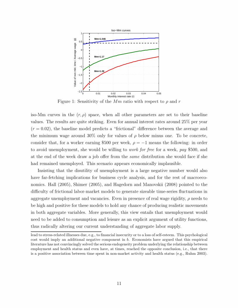
unemployed, over and beyond search effort, is truly very large.12 Figure 1 plots various

10Throughout the paper we only consider models with two employment states. Gautier, Moraga-Gonzales, and Wolthoff (2009) develop a frictional model of the labor market with nonparticipationdriven by shocks to job-search cost. They report that our key findings arise in that environment as well.

11In the model, the unemployed agent optimally chooses λu by trading-off the direct disutility ofsearch cu (λu), and the returns from choosing a higher contact rate. We follow Christensen et al. (2005)

in selecting the isoelastic functional form for the search cost cu (λu) = κuλ1+1/γu where κu is a scaling

constant. In Section 7 we extend our analysis to a version of this model with on-the-job search.12A number of authors in the health and social behavioral sciences have argued that unemployment can

10

0 0.01 0.02 0.03 0.04 0.05−2.5

−2

−1.5

−1

−0.5

0

0.5

1

Monthly interest rate (r)

Val

ue o

f non

mkt

. tim

e / A

vera

ge w

age

(ρ)

Iso−Mm curves

Mm=1.046

Mm=1.17

Mm=1.28

Figure 1: Sensitivity of the Mm ratio with respect to ρ and r

iso-Mm curves in the (r, ρ) space, when all other parameters are set to their baseline

values. The results are quite striking. Even for annual interest rates around 25% per year

(r = 0.02), the baseline model predicts a “frictional” difference between the average and

the minimum wage around 30% only for values of ρ below minus one. To be concrete,

consider that, for a worker earning $500 per week, ρ = −1 means the following: in order

to avoid unemployment, she would be willing to work for free for a week, pay $500, and

at the end of the week draw a job offer from the same distribution she would face if she

had remained unemployed. This scenario appears economically implausible.

Insisting that the disutility of unemployment is a large negative number would also

have far-fetching implications for business cycle analysis, and for the rest of macroeco-

nomics. Hall (2005), Shimer (2005), and Hagedorn and Manovskii (2008) pointed to the

difficulty of frictional labor-market models to generate sizeable time-series fluctuations in

aggregate unemployment and vacancies. Even in presence of real wage rigidity, ρ needs to

be high and positive for these models to hold any chance of producing realistic movements

in both aggregate variables. More generally, this view entails that unemployment would

need to be added to consumption and leisure as an explicit argument of utility functions,

thus radically altering our current understanding of aggregate labor supply.

lead to stress-related illnesses due, e.g., to financial insecurity or to a loss of self-esteem. This psychologicalcost would imply an additional negative component in b. Economists have argued that this empiricalliterature has not convincingly solved the serious endogeneity problem underlying the relationship betweenemployment and health status and even have, at times, reached the opposite conclusion, i.e., that thereis a positive association between time spent in non-market activity and health status (e.g., Ruhm 2003).

11

3.2 Taking stock

When plausibly calibrated to match labor-market flows the baseline search model implies

that wage differentials arising among similar workers purely because of search frictions

are very small. Intuitively, frictional wage dispersion in search models is constrained by

the size of worker flows. Our sensitivity analysis establishes the robustness of this finding.

Only with large and negative values of non market time will the model predict sizeable

Mm ratios while remaining consistent with the observed unemployment duration. Even

though direct knowledge of this parameter is scant, we argued that negative values of ρ

are economically implausible.

The baseline model relies on 1) perfect correlation between job values and initial wages,

2) risk neutrality, 3) random search, and 4) no on-the-job search. In the rest of the paper,

we relax these four key assumptions one by one. These extensions allows us to inspect

some of the most recent contributions to the search literature.

4 Imperfect correlation between job values and wages

There are three main reasons why the initial wage drawn by the unemployed worker may

not map one for one into the corresponding job value.

Compensating differentials Wages are only one component of total compensation.

In a search model where a job offer is a bundle of a wage and other amenities, short

unemployment duration can coexist with large wage dispersion, as long as non-wage job

attributes are negatively correlated with wages so that the dispersion of total job values

is indeed small.

This hypothesis, which combines the theory of compensating differentials with search

theory, does not show too much promise. First, it is well known that certain key non-

wage benefits such as health insurance tend to be positively correlated with the salary,

e.g., through firm size.13 Similarly, layoff rates are larger for low-paid jobs (see Pin-

heiro and Vissers, 2006 for a survey of the evidence). Second, illness or injury risks are

very occupation-specific and consumption deflators are very location-specific, while our

implications for frictional wage dispersion apply to labor markets narrowly defined by

occupational and geographical boundaries. Third, differences in work shifts and part-

time penalties are quantitatively small. Kostiuk (1990) shows that genuine compensating

13For example, the mean wage in jobs offering health insurance coverage is 15%-20% higher than inthose not offering it; see Dey and Flinn (2008).

12

differentials between day and night shifts can explain at most 9% of wage gaps in se-

lected occupations. Manning and Petrongolo (2005) calculate that part-time penalties for

observationally similar workers are around 3%.14

Stochastic wages If wages fluctuate randomly on the job, the initial wage offer is not

a good predictor of the continuation value of employment. Since employment maintains

an option value, unemployed workers will be more willing to accept initially low wage

offers, which reduces the reservation wage w∗ and increases frictional dispersion.

In the Technical Appendix we develop an extension of the baseline model where

unemployed workers draw wage offers from the distribution F (w) at rate λu, but now

these wage offers are not permanent. At rate δ, the employed worker draws again from

F (w). Draws are i.i.d. over time. Separations are now endogenous and will occur at rate

σ∗ ≡ δF (w∗).15 In this model, the Mm ratio becomes

Mm =

λ∗

u−δ+σ∗

r+δ+ 1

λ∗

u−δ+σ∗

r+δ+ ρ

. (5)

As δ → 0, the Mm ratio converges to equation (2) with σ∗ = 0, since without any shock

during employment every job lasts forever. As δ → λu, unemployed workers accept every

offer above b since being on the job has an option value equal to being unemployed.

The parameter δ maps into the degree of persistence of the wage process during a job

spell. In particular, in a discrete time model where δ ∈ (0, 1) the autocorrelation coefficient

of the wage process is 1− δ.16 Longitudinal data offer overwhelming evidence that wages

are very persistent, indeed near a random walk at annual frequency, so plausible values of

δ are close to zero.17 In conclusion, adding wage randomness with plausible persistence

has negligible impact on the size of frictional dispersion in search models.18

14Recently, Bonhomme and Jolivet (2009) have estimated a search model where a job has several non-wage attributes (commuting, working times, job security, etc...) beyond its monetary compensation andfind that they command insignificant compensating differentials, which are often found to be of the wrongsign.

15The setup of Mortensen and Pissarides (1994) is similar to that described here, with one difference:upon employment, all workers start with the highest wage, wmax, and thus they only sample from F (w)while employed. In the Technical Appendix we show that the resulting Mm ratio for the Mortensen-Pissarides model is strictly bounded above by that in equation (5) below.

16In the Technical Appendix we also show that a discrete time version of this model leads exactly toequation (5) .

17Even for an autocorrelation of 0.5 at annual frequency—undoubtedly a lower bound for persistence—the monthly value for δ would be 0.056 implying a Mm ratio of 1.084 (in the baseline, Mm = 1.046).

18Recently, Alvarez and Shimer (2009) encounter this problem in a Lucas-Prescott-style environmentwhere each island/industry has a very persistent wage process. In order to match the observed industrywage differentials in the cross section, they are forced to assume huge search costs (i.e., ρ negative).

13

Returns to experience If workers accumulate experience during employment, then

the value of the job has a dynamic component untied to the current payoff. An unemployed

worker is willing to lower her reservation wage in exchange for such long-term gains,

i.e., she is willing to pay for work experience. This environment can generate a larger

Mm ratio. Consider a version of the baseline search model where, during employment,

experience h is expected to grow at the instantaneous rate η. Earnings for the worker are

wh, i.e., the wage offered by hiring firms is per unit of experience. In order to bound the

growth of experience, we must assume that individuals quit the labor force at rate φ.

In the Technical Appendix, we show that in this economy the mean-min ratio of wages

per unit of experience (hence among similar workers) is given by

Mm =

λ∗

u

r+φ+σ−η+ 1

1−η/(r+φ)

λ∗

u

r+φ+σ−η+ ρ

, (6)

an expression that includes (2) as a special case when φ = η = 0. The Mm rises with

returns to experience η, as expected.19

We set the average duration of working life to 40 years, and assume that wages grow

by a factor of 2 over the working life because of accumulated experience. Both values are

fairly uncontroversial. At a monthly frequency, this parameterization implies φ = 0.0021

and η = 0.0017. Plugging these two values, together with those in Section 3, in equation

(6) yields Mm = 1.076. Even though frictional wage dispersion almost doubles, it remains

small in absolute value.

5 Risk aversion

Risk-averse workers particularly dislike states with low consumption, like unemployment.

Compared to risk-neutral workers, ceteris paribus, they lower their reservation wage in

order to exit unemployment rapidly, thus allowing Mm to increase.

No storage Let u (c) be the utility of consumption, with u′ > 0, and u′′ < 0. To make

progress analytically, we assume that workers have no access to storage, i.e., c = w when

employed, and c = b when unemployed. It is clear that this model will give an upper bound

for the role of risk aversion: with any access to storage, self-insurance or borrowing, agents

can better smooth consumption, thus becoming effectively less risk-averse.

19This expression is related to that uncovered by Burdett, Carrillo-Tudela and Coles (2009). Theyincorporate these same considerations in a version of the Burdett and Mortensen (1998) model of on-the-job search. They derive a closed-form expression for the Mm ratio which, as ours, clearly shows thatqualitatively returns to experience can increase frictional wage dispersion.

14

2 4 6 8 10 12 140

0.1

0.2

0.3

0.4

0.5

0.6

0.7

0.8

0.9

Relative risk aversion (θ)

Val

ue o

f non

mkt

. tim

e / A

vera

ge w

age

(ρ)

Iso−Mm curves

Mm=1.20

Mm=1.47

Mm=1.88

Figure 2: Sensitivity of the Mm ratio with respect to ρ and risk aversion

With risk averse agents, in the Bellman equations for the value of employment and

unemployment, the monetary flow values of work and leisure are simply replaced by their

corresponding utility values. The reservation-wage equation (1) then becomes

u (w∗) = u (ρw) +λ∗

u

r + σ[Ew∗ [u (w)] − u (w∗)] , (7)

with Ew∗ [u (w)] = E [u (w) |w ≥ w∗]. In the Technical Appendix, we show how to obtain

the approximation

Mm ≃

[

λ∗

u

r+σ

(

1 + 12(θ − 1) θcv2

)

+ ρ1−θ

λ∗

u

r+σ+ 1

]1

θ−1

(8)

of the mean-min ratio for a CRRA utility function u (w) with coefficient of relative risk

aversion θ and a wage distribution with coefficient of variation cv. It is immediate to see

that, for θ = 0, the risk-neutrality case, the expression above equals that in equation (2) .

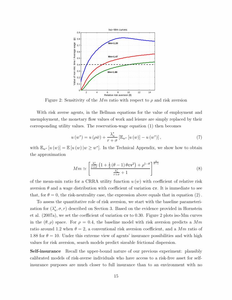
To assess the quantitative role of risk aversion, we start with the baseline parameteri-

zation for (λ∗

u, σ, r) described on Section 3. Based on the evidence provided in Hornstein

et al. (2007a), we set the coefficient of variation cv to 0.30. Figure 2 plots iso-Mm curves

in the (θ, ρ) space. For ρ = 0.4, the baseline model with risk aversion predicts a Mm

ratio around 1.2 when θ = 2, a conventional risk aversion coefficient, and a Mm ratio of

1.88 for θ = 10. Under this extreme view of agents’ insurance possibilities and with high

values for risk aversion, search models predict sizeable frictional dispersion.

Self-insurance Recall the upper-bound nature of our previous experiment: plausibly

calibrated models of risk-averse individuals who have access to a risk-free asset for self-

insurance purposes are much closer to full insurance than to an environment with no

15

storage (see, e.g., Aiyagari, 1994).20 In such models, workers choose their precautionary

savings so that their marginal utility in equilibrium becomes near constant, and hence

wage (and other) outcomes are close to those in a model with linear utility. This obser-

vation severely limits risk aversion as a source of large frictional wage dispersion. For

example, Krusell, Mukoyama, and Sahin (2009) embed the Pissarides (1985) matching

model into an economy where individual unemployment risk is uninsurable. Households

can save through a risk-free asset, but borrowing is precluded. Differences in outside

options related to cross-sectional wealth inequality induce wage dispersion among ex-ante

equal workers through Nash bargaining. However, wage dispersion introduced through

this channel remains extremely small for reasonable calibrations.21

6 Directed search

The directed search model (Moen, 1997) provides an important alternative view to random

search. The model assumes that firms post wages, unemployed workers observe all the

wages offered and direct their search towards the most attractive firms. A higher wage

attracts more applicants to the job. In turn, more applicants means a lower contact rate

for the unemployed. Therefore, in directing their search, workers trade-off higher wages

with longer expected unemployment durations and, in equilibrium, they are indifferent

about where to apply.

As in all other derivations, to characterize the Mm ratio in this model we do not need

to make any assumption on firms’ wage-posting behavior. It suffices to focus on workers’

search behavior. Consider the value for an unemployed worker directing her search to

firm i, rUi = b + λi (Wi − Ui), where λi is the worker’s contact rate. If hired by firm i,

the value of employment for this worker is rWi = wi − σ (Wi − U), where wi is the wage

promised by the hiring firm. Combining these two equations yields

rUi =b (r + σ) + λiwi

r + σ + λi

= rU,

where the second equality is the equilibrium condition requiring unemployed workers to

be indifferent about where to direct their search.

20For example, it is well known that as r → 0, the bond economy with “natural debt limits” convergesto complete markets (Levine and Zame, 2002).

21In the Technical Appendix, we study a sequential search environment where workers with CARApreferences can borrow and save through a riskless asset. The CARA assumption allows to derive theMm ratio in closed form. The quantitative predictions of this model for frictional wage dispersion arevery similar to the risk-neutral case, even with a relative risk aversion of ten.

16

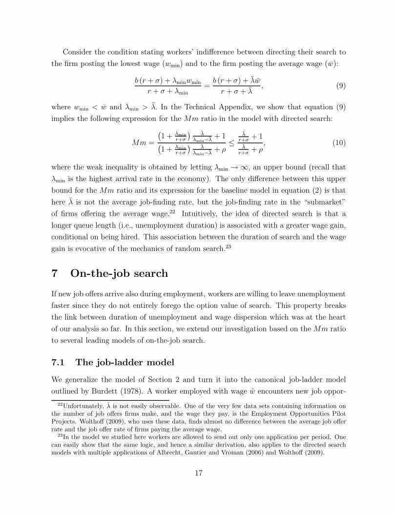
Consider the condition stating workers’ indifference between directing their search to

the firm posting the lowest wage (wmin) and to the firm posting the average wage (w):

b (r + σ) + λminwmin

r + σ + λmin=

b (r + σ) + λw

r + σ + λ, (9)

where wmin < w and λmin > λ. In the Technical Appendix, we show that equation (9)

implies the following expression for the Mm ratio in the model with directed search:

Mm =

(

1 + λmin

r+σ

)

λλmin−λ

+ 1(

1 + λmin

r+σ

)

λλmin−λ

+ ρ≤

λr+σ

+ 1

λr+σ

+ ρ, (10)

where the weak inequality is obtained by letting λmin → ∞, an upper bound (recall that

λmin is the highest arrival rate in the economy). The only difference between this upper

bound for the Mm ratio and its expression for the baseline model in equation (2) is that

here λ is not the average job-finding rate, but the job-finding rate in the “submarket”

of firms offering the average wage.22 Intuitively, the idea of directed search is that a

longer queue length (i.e., unemployment duration) is associated with a greater wage gain,

conditional on being hired. This association between the duration of search and the wage

gain is evocative of the mechanics of random search.23

7 On-the-job search

If new job offers arrive also during employment, workers are willing to leave unemployment

faster since they do not entirely forego the option value of search. This property breaks

the link between duration of unemployment and wage dispersion which was at the heart

of our analysis so far. In this section, we extend our investigation based on the Mm ratio

to several leading models of on-the-job search.

7.1 The job-ladder model

We generalize the model of Section 2 and turn it into the canonical job-ladder model

outlined by Burdett (1978). A worker employed with wage w encounters new job oppor-

22Unfortunately, λ is not easily observable. One of the very few data sets containing information onthe number of job offers firms make, and the wage they pay, is the Employment Opportunities PilotProjects. Wolthoff (2009), who uses these data, finds almost no difference between the average job offerrate and the job offer rate of firms paying the average wage.

23In the model we studied here workers are allowed to send out only one application per period. Onecan easily show that the same logic, and hence a similar derivation, also applies to the directed searchmodels with multiple applications of Albrecht, Gautier and Vroman (2006) and Wolthoff (2009).

17

tunities w at rate λe. These opportunities are randomly drawn from the wage-offer distri-

bution F (w) and they are accepted if w > w. A large class of equilibrium wage-posting

models with random search, starting from the seminal work by Burdett and Mortensen

(1998), derives the optimal wage policy of the firms and the implied equilibrium wage-offer

distribution as a function of structural parameters. As for our analysis in Section 2, it is

not necessary, at any point in our derivations, to specify what F looks like; our expression

for Mm will hold for any F as long as every worker (employed or unemployed) faces the

same wage-offer distribution. Without loss of generality, to simplify the algebra, we posit

that no firm would offer a wage below the reservation wage w∗; thus, F (w∗) = 0.

In the Technical Appendix, we show that under these assumptions the reservation-

wage equation becomes

w∗ = b + (λu − λe)

∫ wmax

w∗

1 − F (z)

r + σ + λe [1 − F (z)]dz. (11)

It is easy to see that, in steady state, the cross-sectional wage distribution among employed

workers is

G (w) =σF (w)

σ + λe [1 − F (w)]. (12)

Using this relation between G (w) and F (w) in the reservation-wage equation (11), and

exploiting the fact that the average wage is

w = w∗ +

∫ wmax

w∗

[1 − G(z)] dz, (13)

we arrive at the new expression for the Mm ratio,

Mm ≃λu−λe

r+σ+λe+ 1

λu−λe

r+σ+λe+ ρ

, (14)

in the model with on-the-job search. The details of this derivation are in the Technical

Appendix.24

Since the Mm ratio is increasing in λe, the model with on-the-job search will generate

more frictional wage inequality than the baseline model. In the extreme case where the

search technology is the same in both employment states and λe = λu, the reservation

24In particular, the “approximately equal” sign originates from one step of the derivation where wehave set

r + σ

r + σ + λe [1 − F (z)]≈

σ

σ + λe [1 − F (z)],

a valid approximation since, for plausible calibrations, r is negligible compared to σ.

18

0.05 0.10 0.15 0.20 0.250.01

0.015

0.02

0.025

0.03

0.035

0.04

0.045

0.05Job−to−Job flows

Mon

thly

EE

rat

e

Monthly offer arrival rate on the job ( λe )

0.05 0.1 0.15 0.2 0.25−2

−1.5

−1

−0.5

0

0.5

Iso−Mm Curves

Monthly offer arrival rate on the job ( λe )

Val

ue o

f non

−m

kt ti

me

(ρ)

EE rate=0.032

EE rate=0.022

Mm=1.16

Mm=1.27 Mm=1.55

Figure 3: Sensitivity of the Mm ratio with respect to ρ and λe

wage will be equal to b, since searching when unemployed gives no better arrival rate of

new job offers, and Mm = 1/ρ.

The crucial new parameter of this model is the arrival rate of offers on the job λe. To

pin down λe, note that the average employment-to-employment (EE) transition rate χ in

the model is given by the expression

χ = λe

∫

w∗

[1 − F (w)] dG (w) =σ (λe + σ) log

(

σ+λe

σ

)

λe− σ. (15)

For a given a value of the employment-to-unemployment (EU) flow rate σ, there is a

one-to-one mapping between χ and λe. The most recent empirical evidence sets monthly

job-to-job flows χ between 2.2% and 3.2% of employment. From SIPP data, Nagypal

(2008, Table 6) sets χ to 2.2%. Based on monthly CPS data, Fallick and Fleischman

(2004) estimate χ = 2.7%, and Nagypal (2008, Table 4) estimates χ = 2.9%. Moscarini

and Vella (2008) argue that a different treatment of missing records in the monthly CPS

leads to an upward revision of χ up to 3.2%.25

In what follows, we ask how much frictional wage inequality the canonical on-the-job

search model predicts, in terms of the Mm ratio, while at the same time being consistent

with the labor-market transitions between employment and unemployment discussed in

Section 3 and, in addition, a monthly job-to-job transition rate between 2.2% and 3.2%.

Figure 3 illustrates that the model with on-the-job search predicts a significantly

larger frictional component of wage dispersion. Once λe is chosen so that the model can

25Maintaining that σ = 0.03, SIPP and CPS imply a total monthly separation rate between 5.2% and6.2%. Estimates of worker flows from JOLTS are roughly consistent with this range. Davis et al. (2008)develop a method to improve statistics of worker flows based on raw survey data from JOLTS, and arriveat a monthly separation rate around 5% in 2000.

19

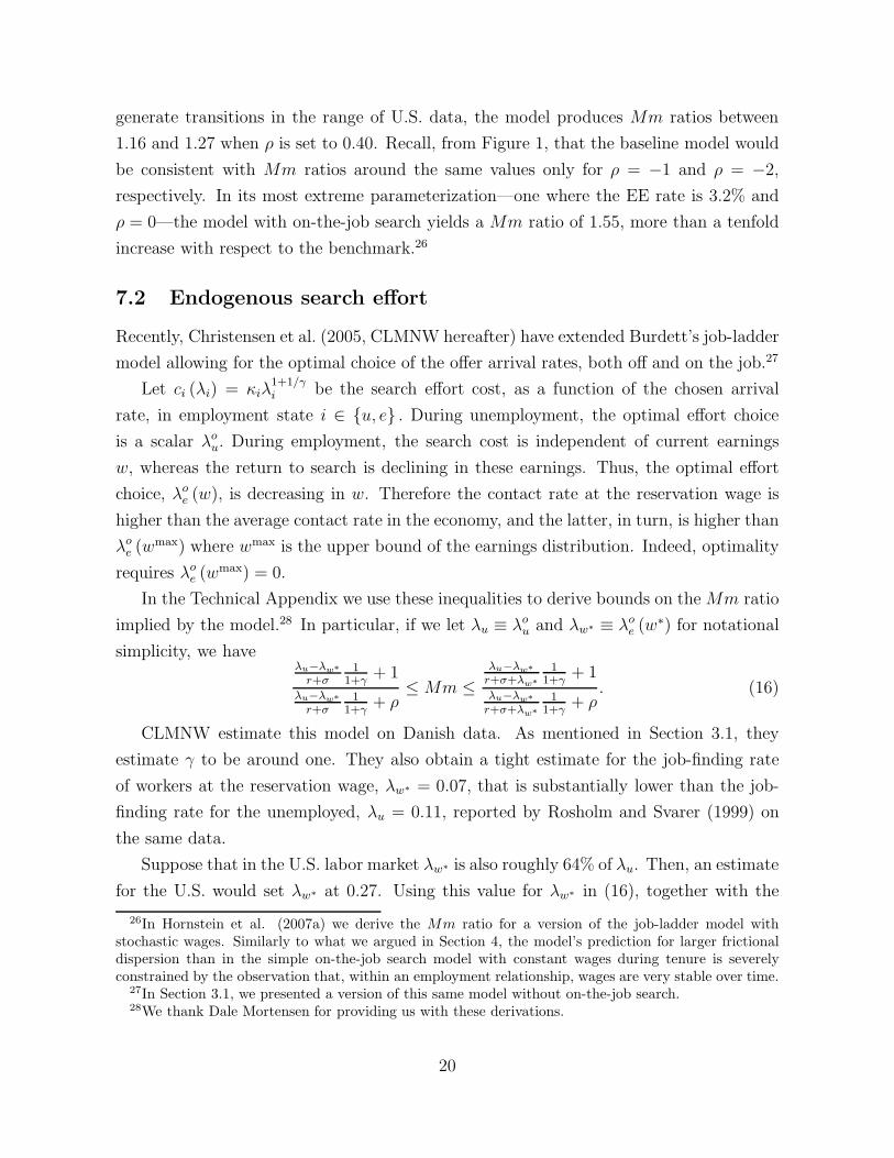
generate transitions in the range of U.S. data, the model produces Mm ratios between

1.16 and 1.27 when ρ is set to 0.40. Recall, from Figure 1, that the baseline model would

be consistent with Mm ratios around the same values only for ρ = −1 and ρ = −2,

respectively. In its most extreme parameterization—one where the EE rate is 3.2% and

ρ = 0—the model with on-the-job search yields a Mm ratio of 1.55, more than a tenfold

increase with respect to the benchmark.26

7.2 Endogenous search effort

Recently, Christensen et al. (2005, CLMNW hereafter) have extended Burdett’s job-ladder

model allowing for the optimal choice of the offer arrival rates, both off and on the job.27

Let ci (λi) = κiλ1+1/γi be the search effort cost, as a function of the chosen arrival

rate, in employment state i ∈ {u, e} . During unemployment, the optimal effort choice

is a scalar λou. During employment, the search cost is independent of current earnings

w, whereas the return to search is declining in these earnings. Thus, the optimal effort

choice, λoe (w), is decreasing in w. Therefore the contact rate at the reservation wage is

higher than the average contact rate in the economy, and the latter, in turn, is higher than

λoe (wmax) where wmax is the upper bound of the earnings distribution. Indeed, optimality

requires λoe (wmax) = 0.

In the Technical Appendix we use these inequalities to derive bounds on the Mm ratio

implied by the model.28 In particular, if we let λu ≡ λou and λw∗ ≡ λo

e (w∗) for notational

simplicity, we haveλu−λw∗

r+σ1

1+γ+ 1

λu−λw∗

r+σ1

1+γ+ ρ

≤ Mm ≤

λu−λw∗

r+σ+λw∗

11+γ

+ 1λu−λw∗

r+σ+λw∗

11+γ

+ ρ. (16)

CLMNW estimate this model on Danish data. As mentioned in Section 3.1, they

estimate γ to be around one. They also obtain a tight estimate for the job-finding rate

of workers at the reservation wage, λw∗ = 0.07, that is substantially lower than the job-

finding rate for the unemployed, λu = 0.11, reported by Rosholm and Svarer (1999) on

the same data.

Suppose that in the U.S. labor market λw∗ is also roughly 64% of λu. Then, an estimate

for the U.S. would set λw∗ at 0.27. Using this value for λw∗ in (16), together with the

26In Hornstein et al. (2007a) we derive the Mm ratio for a version of the job-ladder model withstochastic wages. Similarly to what we argued in Section 4, the model’s prediction for larger frictionaldispersion than in the simple on-the-job search model with constant wages during tenure is severelyconstrained by the observation that, within an employment relationship, wages are very stable over time.

27In Section 3.1, we presented a version of this same model without on-the-job search.28We thank Dale Mortensen for providing us with these derivations.

20

values for the other parameters already discussed in the paper, we obtain a lower bound

of 1.22 and an upper bound of 1.90 for Mm. Therefore, it appears that the model could

be consistent with a large amount of frictional wage dispersion.

How large is the value of non-market time, net of search costs, implied by this pa-

rameterization? Recall from Section 3.1 that search costs, which make unemployment

unattractive relative to employment, can be thought of as lowering ρ. The bounds on

the Mm ratio, together with the first-order condition for optimal search effort during

unemployment, allow us to construct bounds for the search cost during unemployment

cu (λu) as a fraction of the average wage w. In the Technical Appendix, we show that

λu

r + σ + λw∗

γ

1 + γ

(

1 −1

Mm

)

≤cu (λu)

w≤

λu

r + σ

γ

1 + γ

(

1 −1

Mm

)

. (17)

Assuming an Mm ratio of 1.56, the average of the two bounds in (16), the inequalities

in (17) yield a lower bound of 0.25 and an upper bound of 2.26 for the normalized search

cost during unemployment. With ρ = 0.4, the implied net-of-search-cost value of non-

market time (ρ − cu (λu)) /w is then close to zero or, most likely, largely negative.

This calculation echoes one of the central observations of our paper: even with on-the-

job search, sizeable frictional dispersion hinges upon a large disutility of unemployment.

7.3 Sequential auctions and wage-tenure contracts

In a series of recent papers, Postel-Vinay and Robin (2002a, 2002b), Dey and Flinn

(2005), and Cahuc et al. (2006) have developed a new search model where firms are

allowed to make counteroffers when one of their employees is contacted by an outside

firm. The competition between the two employers may result either in a job-to-job move

or in a salary increase on the current job, depending on the productivity gap between

the two competing firms. Through the second channel, the wage distribution can fan

out even without a separation occurring. Therefore, this model contains a much weaker

link between wage dispersion and job-to-job flows, which is what prevents the standard

on-the-job search environment from generating large frictional dispersion.29

Consider a simple version of the sequential auction model where all firms have equal

productivity p. The wage determination mechanism is based on Dey and Flinn (2005)

and Cahuc et al. (2006). An unemployed worker extracts a fraction β of the the surplus

from the firm, but an employed worker who is contacted by an outside firm extracts all

29The argument developed in our paper suggests that what would further discipline the amount offrictional wage dispersion in this model is data on the frequency of job offers matched by the currentemployer. Such data, at the moment, is not available.

21

the surplus from the current employer and receives wage w = p. It is easy to see that the

reservation-wage equation (derived in the Technical Appendix) is

w∗ = b +β (r + σ + λu) − (1 − β)λe

r + σ + βλu(p − b) . (18)

This expression implies that, for low values of workers’ bargaining power β, one can

achieve w∗ < b. This is, for example, the case in the Postel-Vinay and Robin (2002a,

2002b) version of the model, where β = 0. As long as λe > 0, the worker expects to earn

a higher wage after she has been hired, and thus she is willing to accept a low entry-wage.

As a result, Mm > 1/ρ.30

Stevens (1999) and Burdett and Coles (2001) generalize the wage-posting model of

Burdett and Mortensen (1998) by allowing employers to offer long-term wage-tenure con-

tracts on a take-it-or-leave-it basis. This long-term wage tenure contract is observationally

equivalent to the wage path arising in the counteroffer model with β = 0. Consider the

same simple economy with homogenous firms, and restrict attention to a family of con-

tracts (w∗, wT , λT ) such that the entrant worker is paid w∗ (optimally determined by the

firm in equilibrium) and then, at rate λT , i.e., after an expected tenure length of 1/λT ,

her wage jumps up to wT . Clearly, an optimal contract that minimizes costly turnover for

the firm sets wT = p. This wage contract is isomorphic to the wage in the counteroffer

model if λT = λe. This equivalence means that in search environments with wage-tenure

contracts, frictional wage dispersion can be large, even allowing Mm > 1/ρ.

Although the sequential auction model is undoubtedly a good representation for cer-

tain high-skill occupations (e.g., academic jobs), it does not appear to be a widespread

mechanism for wage setting in the labor market at large.31 An additional limit of this

model is that, for high values of λe, the entry wage w∗ may be negative.32 The version with

wage-tenure contracts avoids this problem by restricting contracts so that w∗ = ω ∈ (0, b)

with equation (18) determining the expected tenure 1/λT at which the worker sees his

salary increasing to p. A possible drawback of the Stevens-Burdett-Coles model is its heavy

reliance on the assumption that firms can commit to long-term contracts. In practice, it

30Papp (2009) develops a general-equilibrium version of this model with heterogeneous firms and showsthat, once parsimoniously parameterized, it can generate Mm ratios beyond 2.0 for ρ = 0.4 and r set at4% per year, while at the same time being consistent with the empirically observed size of labor-marketflows.

31One reason is that in many labor markets asymmetric information may prevent the firm from beingable to verify the outside offer. See Mortensen (2005) for a discussion of why counteroffers are uncommonin actual labor markets.

32In the Technical Appendix, we show that if β = 0, our baseline calibration would indeed imply thatw∗ < 0, independently of p.

22

appears that renegotiation is frequent.33

Conditional on these question marks, a further analysis of which is beyond the scope

of our paper, this new set of search environments seems to yield sizeable frictional wage

dispersion while, at the same time, matching observed labor-market flows.

8 Relation to structural estimation of search models

Since the pioneering effort of Flinn and Heckman (1983), a rather vast literature on

structural estimation of search models has developed (see Eckstein and van den Berg,

2007, for a recent survey). These contributions have generated many valuable insights on

the functioning of labor markets and on policy analysis. From our perspective though, it is

important to highlight the difficulty that these models have in simultaneously matching

the wage dispersion and labor-market flows with a plausible parameterization without

resorting to measurement error or unobserved skill heterogeneity to soak up the large

wage residuals in the data. We now proceed to discussing a number of examples from the

literature.

In one of the first attempts at a full structural estimation, Eckstein and Wolpin (1990)

estimate the Albrecht and Axell (1984) search model with worker heterogeneity in the

value of non-market productivity and conclude that their model cannot generate any sig-

nificant wage dispersion, and that almost all of the observed wage dispersion is explained

through measurement error. Eckstein and Wolpin (1995) reach a far better match between

model and data, by introducing a five-point distribution of unobserved worker heterogene-

ity within each race/education group (8 groups in total). In spite of such heterogeneity,

however, for many of the groups the estimates of b remain extremely small or negative

(see their Table 7, page 284). In this work, thus, wage dispersion is for the most part

accounted for by heterogeneity in observable and unobservable characteristics. In our

view, this procedure, which is quite frequent in this literature, can perhaps be categorized

more as part of the human-capital theory of wages: it delivers wage inequality, but this

inequality is not frictional in nature.34

33Kiyotaki and Lagos (2006) develop an equilibrium model of two-sided, on-the-job search with nocommitment (i.e., with continuous renegotiation) where the worker, even when facing only one employer,always has the chance of making a take-it-or-leave-it offer with a fixed probability.

34A theoretical argument has also been raised against this kind of model of frictional wage dispersion.Gaumont et al. (2006) demonstrate that wage dispersion in an Albrecht and Axell (1984) model withworker heterogeneity in the value of leisure is fragile. As soon as an arbitrarily small search cost isintroduced, the equilibrium unravels and we are back to the “Diamond paradox”, i.e., to an equilibriumwith a unique wage.

23

Negative estimates of the net value of non market time are quite common. The survey

paper by Bunzel et al. (2001) estimates several models with on-the-job search on Danish

data. When firms are assumed to be homogeneous, the point estimate for ρ is −2. With

heterogeneity in firms’ productivity it increases to just about zero. Only the model with

measurement error produces a large and positive estimate of ρ.35 Flinn (2006) estimates

a Pissarides-style matching model of the labor market, without on-the-job search, to

evaluate the impact of the minimum wage on employment and welfare. In his model, as

is typical in estimation exercises, the pair (ρ, r) is not separately identified. Setting r to

5% annually in his model implies roughly ρ = −4.36

An example of extreme parameter estimates can even be found in Postel-Vinay and

Robin (2002a)—an environment that, we argued, has the potential of generating large

frictional dispersion while matching labor market flows. Under risk neutrality, their es-

timates of the discount rate r always exceed 30% per year in every occupational group,

reaching 55% for unskilled workers, where they find no role for unobserved heterogeneity.

Recall, from our analysis of Section 3 that a negative value for ρ and a high value for r

are two sides of the same coin.

Whenever authors restrict (r, ρ) to plausible values ex-ante, not surprisingly in light

of our results, they end up finding that frictions play a minor role. For example, Van den

Berg and Ridder (1998) estimate the Burdett-Mortensen model on Dutch data allowing for

measurement error and observed worker heterogeneity (58 groups defined by education,

age and occupation). They set r to zero and b to equal unemployment benefits for each

group, i.e., roughly 60% of the average wage. They conclude that observed heterogeneity

and measurement error account for over 80% of the empirical wage variation. Moscarini

(2003, 2005) develops an equilibrium search model where workers learn about their match

values, based on Jovanovic (1979). When the model is calibrated, r is set to 5% annually

and ρ to 0.6. His model generates a Mm ratio of just 1.16 (Moscarini, 2003, Table 2).

A number of papers in the literature claim that the (on-the-job search) model is suc-

cessful in simultaneously matching both the wage distribution and labor-market transition

data (see, e.g., Bontemps et al., 2000; Jolivet et al., 2005). These claims of success need

to be properly reinterpreted in light of our findings. The typical strategy in these papers

is, first, to estimate the employment wage distribution G(w) non-parametrically without

using the search model. Next, the model is used to predict the wage-offer distribution

F (w) through a steady-state relationship like (12), where the structural parameters of

35These values for ρ are obtained from Bunzel et al. (2001) by dividing the estimates of b for the entiresample, in Tables II and V, by the average wage from Table I.

36Calculations are available upon request.

24

the relationship (σ, λu, λe) are estimated by matching transition data. Success is then

expressed as a good fit (in some specific metric). However, the exercise is incomplete

because it neglects the implications of the joint estimates of F (w) and of the transition

parameters for the relative value of non-market time ρ (or, similarly, for the interest rate

r). The key additional “test” that we are advocating would thus entail using the estimated

F (w) in the reservation-wage equation (11) and, given an estimate of w∗ (for example,

the bottom-percentile wage observed), backing out the implied value for ρ. In light of our

results, we maintain that ρ would be often negative or close to zero.

In conclusion, while we recognize substantial progress in this literature, the success is

often only partial when it relies on “free parameters”. In short, important parameters,

such as the value of non-market time and the discount rate, respectively, are considered

free parameters, i.e., values that are far from what we view as plausible are routinely

“accepted” in the estimation. Alternatively, unobserved heterogeneity or measurement

error must be introduced, with amounts that are also free parameters, in order to match

the data. Our contribution in this context is to show that, through the lenses of the

mean-min ratio, one can organize many seemingly puzzling and unrelated findings in the

literature on structural estimation of search models in a unified way.

9 Conclusions

Search theory maintains that similar workers looking for jobs in the same labor market

may end up earning different wages according to their luck in the search process. The

resulting wage dispersion has a “frictional” nature. An important question in macroeco-

nomics and labor economics is: how large is this component of wage inequality empiri-

cally? This paper has proposed a simple, but widely applicable, structural method for

quantifying the frictional component of wage dispersion predicted by search models. The

strategy is based on a particular measure of wage differentials, the mean-min ratio, that

arises very naturally, in closed form, from the reservation-wage equation, the cornerstone

of a vast class of search models. A key property of our proposed metric is that it does not

require any knowledge about the wage-offer distribution, and its derivation is independent

of the specific equilibrium mechanism underlying the wage-offer distribution.

We begin by proving that, when plausibly calibrated to match labor-market transition

data, the textbook search model (perfect correlation between wage and job value, risk

neutrality, random search, no on-the-job search) would imply that frictions play virtually

no role in determining wage inequality among ex-ante similar workers: the mean-min wage

25

ratio is less than 1.05. In the remainder of the paper we then relax the key assumptions

of the canonical model one by one. While most of these generalized models predict larger

frictional wage dispersion, in absolute terms its size remains small. However, the most

recent developments of on-the-job-search models, including those with endogenous search

effort, sequential auctions among competing employers, and firm posting of wage-tenure

contracts, seem to more easily accommodate sizeable frictional wage dispersion with labor-

market flows of the observed magnitude.

The mean-min ratio also turns out to be a valuable tool for interpreting the findings

in the literature. In particular, it allows us to interpret a number of arguably enigmatic

and unrelated findings within the literature that structurally estimates search models—

notably, the necessity to tolerate large measurement error, sizeable unobserved workers’

heterogeneity, or implausible parameter values needed in order to jointly account for both

transition and wage data.

A far-reaching, and general, implication of our findings is that the smaller the value

of non-market time (denoted ρ above, expressing this benefit as a fraction of the average

wage), the larger the component of cross-sectional wage dispersion that is attributable

to frictions. Recently Hall (2005), Shimer (2005), and Hagedorn and Manovskii (2008)

sparked a debate over the ability of the canonical matching model (Pissarides, 2000)

to generate enough time-series fluctuations in aggregate unemployment and vacancies.

There, it is pointed out that the model requires a very high ρ in order to produce sharp

movements in vacancy and unemployment rates. Therefore, the time-series facts neces-

sitate a value of ρ close to one to explain the data, and cross-sectional facts demand a

value of ρ below zero.37 It is paramount, in future work, to keep this tension between

time series and cross-section in mind while developing and using frictional theories of the

labor market.

37Building on our insight, Bils, Chang, and Kim (2010) explore this trade-off in the Mortensen-Pissarides (1994) version of the matching model with aggregate and idiosyncratic shocks, and find thatit jeopardizes its performance: the model cannot produce both realistic cross-sectional wage dispersionand realistic cyclical fluctuations in unemployment.

26

References

[1] Acemoglu, D. (2002). “Technical Change, Inequality, and the Labor Market,” Journal ofEconomic Literature, vol. 40(1), pages 7–72.

[2] Autor, D., L. Katz, and M. Kerney (2008). “Trends in U.S. Wage Inequality: Revising theRevisionists,” Review of Economics and Statistics, vol. 90(2), pages 300–323.

[3] Aiyagari, R. (1994). “Uninsured Idiosyncratic Risk and Aggregate Saving,” Quarterly Jour-nal of Economics, vol. 109(3), pages 659-684.

[4] Albrecht J., and B. Axell (1984). “An Equilibrium Model of Search Unemployment,” Jour-nal of Political Economy, vol. 92, pages 824-840.

[5] Albrecht J., P.A. Gautier, and S. Vroman (2006). “An Equilibrium Directed Search withMultiple Applications,” Review of Economic Studies,vol. 73(4), pages 869–891.

[6] Alvarez F., and R. Shimer (2009). “Search and Rest Unemployment,” mimeo, Universityof Chicago.

[7] Aghion, P. and P. Howitt (1994), “Growth and Unemployment,”Review of Economic Stud-ies, vol. 61, pages 477-494.

[8] Bils, M., Y. Chang, and S.B. Kim (2010). “Worker Heterogeneity and Endogenous Sepa-rations in a Matching Model of Unemployment Fluctuations,”forthcoming, American Eco-nomic Journal: Macroeconomics.

[9] Bonhomme, S. and G. Jolivet (2009). “The Pervasive Absence of Compensating Differen-tials,”Journal of Applied Econometrice, forthcoming.

[10] Bontemps, C., J.-M. Robin, and G. J. Van den Berg (2000). “Equilibrium Search withContinuous Productivity Dispersion Theory and Non Parametric Estimation,” InternationalEconomic Review, vol. 41(2), pages 305-358.

[11] Burdett, K. (1978). “A Theory of Employee Job Search and Quit Rates,” American Eco-nomic Review, vol. 68, pages 212-220.

[12] Burdett, K., C. Carrillo-Tudela, and M. Coles (2009). “Human Capital Accumulation andLabour Market Equilibrium,” mimeo, University of Essex.

[13] Burdett, K. and M. Coles (2000). “Equilibrium Wage-Tenure Contracts,” Econometrica,vol. 71, pages 1377-1404.

[14] Burdett, K., and D. T. Mortensen (1998). “Wage Differentials, Employer Size, and Unem-ployment,” International Economic Review, vol. 39(2), pages 257-273.

[15] Bunzel, H., B. J. Christensen, P. Jensen, N. M. Kiefer, L. Korsholm, L. Muus, G. R.Neumann, and M. Rosholm (2001). “Specification and Estimation of Equilibrium SearchModels,” Review of Economic Dynamics, vol. 4, pages 90-126.

[16] Cahuc, P., F. Postel-Vinay, and J.-M. Robin (2006). “Wage Bargaining with On-the-jobSearch: Theory and Evidence,”Econometrica, vol. 74(2), pages 323-64.

[17] Christensen, B. J., R. Lentz, D. T. Mortensen, G. R. Neumann, and A. Wervatz (2005).“On the Job Search and the Wage Distribution,” Journal of Labor Economics, vol. 23(1),pages 31-58.

[18] Cowell, F. (2000). “Measurement of Inequality,” Handbook of Income Distribution, A.Atkinson and F. Bourgignon eds., North Holland, pages 87-166.

27

[19] Davis S., J. Faberman, J. Haltiwanger, and I Rucker (2008). “Adjusted Estimates of WorkerFlows and Job Openings in JOLTS,”NBER WP 14137.

[20] Dey, M. and C. Flinn (2005). “An Equilibrium Model of Health Insurance Provision andWage Determination,” Econometrica, vol. 73(2), pages 571-627.

[21] Dey, M. and C. Flinn (2008). “Household Search and Health Insurance Coverage,” Journalof Econometrics, vol. 145(1-2), pages 43-63.

[22] Eckstein, Z., and G. Van den Berg (2007). “Empirical Labor Search: A Survey,” Journalof Econometrics, vol. 136(2), pages 531-564.

[23] Eckstein, Z., and K. Wolpin (1990). “Estimating a Market Equilibrium Search Model fromPanel Data on Individuals,” Econometrica, vol. 4, pages 783-808.

[24] Eckstein, Z., and K. Wolpin (1995). “Duration to First Job and the Return to Schooling:Estimates from a Search-Matching Model,” Review of Economic Studies, vol. 62, pages263-286.

[25] Fallick, B. and C. A. Fleischman (2004). “Employer-to-Employer Flows in the U.S. LaborMarket: The Complete Picture of Gross Worker Flows,” Finance and Economics DiscussionSeries 2004-34. Washington: Board of Governors of the Federal Reserve System.

[26] Flinn, C. (2006). “Minimum Wage Effects on Labor Market Outcomes Under Search, Bar-gaining, and Endogenous Contact Rates,” Econometrica, vol. 74, pages 1013-1062.

[27] Flinn, C. and J. Heckman (1983). “Are Unemployment and Out of the Labor Force Be-haviorally Distinct Labor Force States?,” Journal of Labor Economics, vol. 1(1), pages28-42.

[28] Gautier, P. and C. Teulings (2006). “How Large Are Search Frictions?,” Journal of theEuropean Economic Association, vol. 4(6), pages 1193-1225.

[29] Gaumont, D., M. Schindler, and R. Wright (2006). “Alternative Theories of Wage Disper-sion,” European Economic Review, vol. 50(4), pages 831-848.

[30] Hagedorn, M., and I. Manovskii (2008). “The Cyclical Behavior of Equilibrium Unemploy-ment and Vacancies Revisited,” American Economic Review, vol. 98(4), pages 1692-1706.

[31] Hall, R. E. (2005). “Employment Fluctuations with Equilibrium Wage Stickiness,” Ameri-can Economic Review, vol. 95(1), pages 50-65.

[32] Hansen, H. (1998). “Transition from Unemployment Benefits to Social Assistance in SevenEuropean OECD Countries,” Empirical Economics, vol. 23(1), pages 5-30.

[33] Hornstein, A., P. Krusell and G.L. Violante (2007a). “Frictional Wage Dispersion in SearchModels: A Quantitative Assessment,” NBER WP 13674.

[34] Hornstein, A., P. Krusell and G.L. Violante (2007b). “Technology-Policy Interaction inFrictional Labor Markets,” Review of Economic Studies, vol. 74(4), pages 1089-1124.

[35] Hornstein, A., P. Krusell and G.L. Violante (2009). “Technical Appendix for Fric-tional Wage Dispersion in Search Models: A Quantitative Assessment,” available athttp://www.econ.nyu.edu/user/violante/research.htm

[36] Jolivet, G., F. Postel-Vinay and J.-M. Robin (2006). “The Empirical Content of the JobSearch Model: Labor Mobility and Wage Dispersion in Europe and the U.S.,”EuropeanEconomic Review, vol. 50(4), pages 877-907

28

[37] Jovanovic, B. (1979). “Job Matching and the Theory of Turnover,” Journal of PoliticalEconomy, vol. 87(5), pages 972-990.

[38] Kostiuk, P. (1990). “Compensating Differentials for Shift Work,” Journal of Political Econ-omy, vol. 98, pages 1054-1075.

[39] Kiyotaki N., and R. Lagos (2006). “A Model of Job and Worker Flows,” Journal of PoliticalEconomy, vol. 115(5), pages 770-819.

[40] Krusell, P., T. Mukoyama, and A. Sahin (2009). “Labor-Market Matching with Precaution-ary Savings and Aggregate Fluctuations,” Review of Economic Studies, forthcoming.

[41] Lemieux, T. (2006). “Increasing Residual Wage Inequality: Composition Effects, NoisyData, or Rising Demand for Skills?,” American Economic Review, vol. 96(3), pages 461–498.

[42] Levine, D. and W. Zame (2002). “Does Market Incompleteness Matter?” Econometrica,vol. 70(5), pages 1805-1839.

[43] Lucas, R. E., and E. Prescott (1974). “Equilibrium Search and Unemployment,” Journalof Economic Theory, vol. 7(2), pages 188-209.

[44] Machin, S., and A. Manning (1999). “The Causes and Consequences of Long-Term Unem-ployment in Europe,” in Handbook of Labor Economics, (edited by Ashenfelter, O., andD. Card), North-Holland.

[45] Manning, A., and B. Petrongolo (2005). “The Part-Time Pay Penalty,” CEP DiscussionPaper No. 679.

[46] McCall, J. (1970). “Economics of Information and Job Search,” Quarterly Journal of Eco-nomics, vol. 84(1), pages 113-126.

[47] Moen, E. (1997). “Competitive Search Equilibrium,” Journal of Political Economy, vol.105(2), pages 385-41.

[48] Mortensen, D. T. (1970). “Job Search, the Duration of Unemployment, and the PhillipsCurve,” American Economic Review, vol. 60(5), pages 847-62.

[49] Mortensen, D. T. (2005). Wage Dispersion: Why Are Similar Workers Paid Differently?,MIT Press.

[50] Mortensen, D. T., and C. Pissarides (1994). “Job Creation and Job Destruction in theTheory of Unemployment,” Review of Economic Studies, vol. 61(3), pages 397-415.

[51] Mortensen, D.T. and C. Pissarides (1998); “Technological Progress, Job Creation, and JobDestruction,”Review of Economic Dynamics, vol. 1(4), pages 733-53.

[52] Moscarini, G. (2003). “Skill and Luck in the Theory of Turnover,” mimeo, Yale University.

[53] Moscarini, G. (2005) “Job Matching and the Wage Distribution,”Econometrica, vol. 73(2),pages 481-516.

[54] Moscarini, G., and F. Vella (2008). “Occupational Mobility and the Business Cycle,”NBERWP 13819.

[55] Nagypal, E. (2008). “Worker Reallocation Over the Business Cycle: The Importance ofJob-to-Job Transitions,” mimeo, Northwestern University.

[56] Papp, T. (2008). “Explaining Frictional Wage Dispersion,” mimeo, Princeton University.

29

[57] Pinheiro, R. and L. Visschers (2006). “Job Security and Wage Differentials,” mimeo, Uni-versity of Pennsylvania.

[58] Pissarides, C. (1985). “Short-run Equilibrium Dynamics of Unemployment Vacancies, andReal Wages,” American Economic Review, vol. 75(4), pages 676-90.

[59] Pissarides, C. (2000). Equilibrium Unemployment Theory, MIT Press.

[60] Postel-Vinay, F. and J.-M. Robin (2002a). “Equilibrium Wage Dispersion with Worker andEmployer Heterogeneity,” Econometrica, vol. 70(6), pages 2295-2350.

[61] Postel-Vinay, F. and J.-M. Robin (2002b). “The Distribution of Earnings in an EquilibriumSearch Model with State-Dependent Offers and Counteroffers,” International EconomicReview, vol. 43(4), pages 989-1016.

[62] Rogerson, R., R. Shimer, and R. Wright (2006). “Search Theoretic Models of the LaborMarket,” Journal of Economic Literature, vol. 43 (4), pages 959-988.

[63] Rosholm, M. and M. Svarer (2005). “Endogenous Wage Dispersion in a Search-MatchingModel,” Labor Economics, vol. 11(5), pages 623-645.

[64] Ruhm, C. (2003). “Good Times Makes You Sick,” Journal of Health Economics, vol. 22(4),pages 637-658.

[65] Shimer, R. (2005). “The Cyclical Behavior of Equilibrium Unemployment and Vacancies,”American Economic Review, vol. 95(1), pages 25-49.

[66] Shimer, R. (2007a) “Mismatch,” American Economic Review, vol. 97(4), pages 1074-1101.

[67] Shimer, R. (2007b). “Reassessing the Ins and Outs of Unemployment”, mimeo, Universityof Chicago.

[68] Stevens, M. (1999). “Wage-Tenure Contracts in a Frictional Labour Market: Firms’ Strate-gies for Recruitment and Retention,” Reviw of Economic Studies, vol. 71, pages 535-551.

[69] Van den Berg, G., and G. Ridder (1998). “An Empirical Equilibrium Search Model of theLabor Market,” Econometrica, vol. 66(5), pages 1183-1221.

[70] Van den Berg, G., and A. Van Vuuren (2008). “The Effect of Search Frictions onWages,”mimeo, Tinbergen Institute.

[71] Wolthoff, R. (2009). “Applications and Interviews: A Structural Analysis of Two-SidedSimultaneous Search,”mimeo, University of Chicago.

30