Embed Size (px)
Citation preview
HAL Id: hal-00782485https://hal-upec-upem.archives-ouvertes.fr/hal-00782485
Submitted on 29 Jan 2013
HAL is a multi-disciplinary open accessarchive for the deposit and dissemination of sci-entific research documents, whether they are pub-lished or not. The documents may come fromteaching and research institutions in France orabroad, or from public or private research centers.
L’archive ouverte pluridisciplinaire HAL, estdestinée au dépôt et à la diffusion de documentsscientifiques de niveau recherche, publiés ou non,émanant des établissements d’enseignement et derecherche français ou étrangers, des laboratoirespublics ou privés.
Friction and wear during twin-disc experiments underambient and cryogenic conditions
Luc Chevalier, S. Cloupet, M. Quillien
To cite this version:Luc Chevalier, S. Cloupet, M. Quillien. Friction and wear during twin-disc experiments underambient and cryogenic conditions. Tribology International, Elsevier, 2006, 39 (11), pp.1376-1387.�10.1016/j.triboint.2005.12.003�. �hal-00782485�
1
Submitted to Tribology International, Nov. 2004 Revised version, November 2005
Friction and Wear during Twin-disc Experiments under Ambient and Cryogenic
Conditions
L. Chevalier1*, S. Cloupet1, M. Quillien2
1LaM, Université de Marne la Vallée
5 boulevard Descartes
Champs sur Marne
77454 Marne la Vallée Cedex, France
Tel.: (33) 1 60 95 77 85
Email: [email protected]
Email: [email protected]
URL: http://www.univ-mlv.fr/lam/lam.htm
2ISMEP - LISMMA, 3 rue Fernand Hainaut
93407 St Ouen Cedex - France
Tel: (33) 1 49 45 29 55
Email: [email protected]
* corresponding author
2
Friction and Wear during Twin-disc Experiments under Ambient and Cryogenic
Conditions
L. Chevalier, S. Cloupet, M. Quillien
Abstract: We present a classical rolling contact apparatus where two discs roll and slide under
a constant normal loading. Experimental results concerning bearing steel used in ambient air
or under severe temperature conditions (Liquid Nitrogen) are presented. A simplified model
proposed by Kalker (Fastsim) is used to identify the dynamic friction coefficient between
these discs and to study the apparatus parameters influence on dissipated energy. Wear
evolution is simulated using classical Archard’s law and compared to measured profiles.
Influence of ambient conditions is highlighted by comparing friction and wear coefficients.
Keywords: Twin-disc experiment, dynamic friction coefficient measurement, wear simulation,
Fastsim
1. Introduction
Bearing track lubrication limits the dynamic friction coefficient value when the bearing balls
are loaded. Consequently, the wear which results from this friction is also limited. In the case
of turbopump bearings used in the space shuttle launch engine, the important loading makes
this point very sensitive. Moreover, these bearings work in particularly harsh thermal
environments since they are bathed in liquid oxygen (90 K) or liquid hydrogen (20 K). At
such temperatures one is interested to know the effects of friction and wear. Because it is very
difficult to manage lubrication at this temperature, our goal is to study the influence of the
temperature on dynamic friction coefficient and wear factor in the absence of lubrication.
3
Twin disc apparatus is used to perform dynamic friction coefficient evolution measurements
under constant normal load and variable slip (see Quillien & al. [1]). After testing,
information on wear may be obtained. In this study we focus on modelling the experiment in
order to evaluate dynamic friction coefficient and wear factor for the two situations: ambient
temperature and cryogenic conditions (-196°C).
First, we briefly recall the mechanical problem to solve and estimate the tangential force
during the twin-disc experiment. Then we compare the experimental results to the simulation
in order to discuss: (i) the evolution of the apparent friction coefficient versus longitudinal
slip; (ii) the influence of temperature on coefficient of friction. Afterwards, we present the
wear measurements and recall Archard’s law used for simulation. An updated Hertzian
approach is used to take into account the wear profile evolution. Finally, we discuss the
results of the simulation and make conclusions on the wear factor value in cryogenic or
ambient air.
2. Dynamic friction coefficient identification
2.1 Twin-disc apparatus description
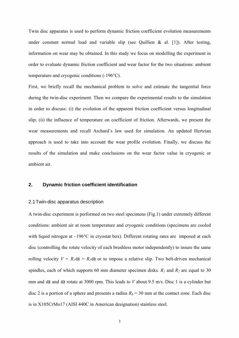
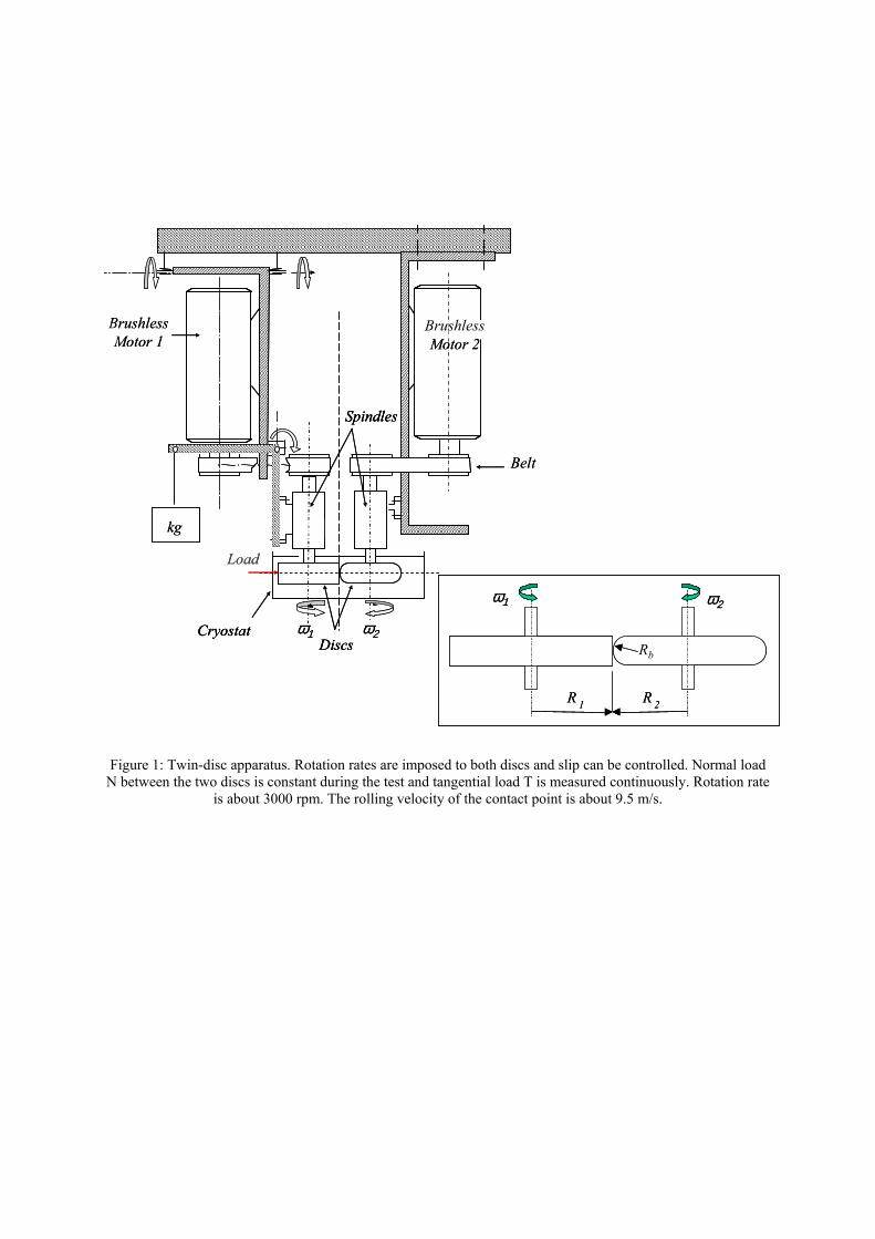
A twin-disc experiment is performed on two steel specimens (Fig.1) under extremely different
conditions: ambient air at room temperature and cryogenic conditions (specimens are cooled
with liquid nitrogen at –196°C in cryostat box). Different rotating rates are imposed at each
disc (controlling the rotate velocity of each brushless motor independently) to insure the same
rolling velocity V = R1ω1 = R2ω2 or to impose a relative slip. Two belt-driven mechanical
spindles, each of which supports 60 mm diameter specimen disks. R1 and R2 are equal to 30
mm and ω1 and ω2 rotate at 3000 rpm. This leads to V about 9.5 m/s. Disc 1 is a cylinder but
disc 2 is a portion of a sphere and presents a radius Rb = 30 mm at the contact zone. Each disc
is in X105CrMo17 (AISI 440C in American designation) stainless steel.
4
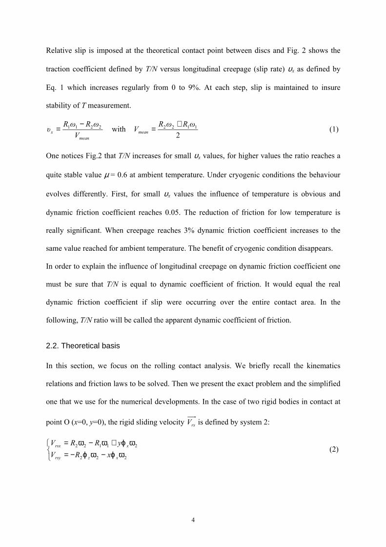
Relative slip is imposed at the theoretical contact point between discs and Fig. 2 shows the
traction coefficient defined by T/N versus longitudinal creepage (slip rate) υx as defined by
Eq. 1 which increases regularly from 0 to 9%. At each step, slip is maintained to insure
stability of T measurement.
2with 11222211 ωRωR
V V
ωRωRυ mean
mean
x
+=
−= (1)
One notices Fig.2 that T/N increases for small υx values, for higher values the ratio reaches a
quite stable value µ = 0.6 at ambient temperature. Under cryogenic conditions the behaviour
evolves differently. First, for small υx values the influence of temperature is obvious and
dynamic friction coefficient reaches 0.05. The reduction of friction for low temperature is
really significant. When creepage reaches 3% dynamic friction coefficient increases to the
same value reached for ambient temperature. The benefit of cryogenic condition disappears.
In order to explain the influence of longitudinal creepage on dynamic friction coefficient one
must be sure that T/N is equal to dynamic coefficient of friction. It would equal the real
dynamic friction coefficient if slip were occurring over the entire contact area. In the
following, T/N ratio will be called the apparent dynamic coefficient of friction.
2.2. Theoretical basis
In this section, we focus on the rolling contact analysis. We briefly recall the kinematics
relations and friction laws to be solved. Then we present the exact problem and the simplified
one that we use for the numerical developments. In the case of two rigid bodies in contact at
point O (x=0, y=0), the rigid sliding velocity rsV is defined by system 2:
ωϕ−ωϕ−=ωϕ+ω−ω=
222
21122
xzrsy
xrsx
xRV
yRRV (2)
5
Where rsxV and rsyV are the x-coordinate and y-coordinate of rsV , φx and φz are angular
defects between the two bodies. Since bodies have an elastic behaviour, the relative velocity
has a complementary term and system 2 becomes:
∂∂−−−=
∂∂−+−=
x
yxvVxRw
x
yxuVyRRw
xzy
xx
),(
),(
222
21122
ωϕωϕ
ωϕωω (3)
Where ),( yxwr
is the sliding velocity between two elastic bodies and wx and wy its
components. u(x,y) and v(x,y) are the relative displacements in x-direction and y-direction. w
can be divided by V and system (3) becomes:
∂∂−φ+υ=
∂∂−φ−υ=
),(
),(
x
yxvx
V
wx
yxuy
V
w
y
y
x
x
with
ωϕ=φ
ωϕ−=υ
V
V
R
x
zy
2
22
(4)
υx and υy are called longitudinal (υx is also usually called “slip rate”) and lateral creepages, φ
is the spin in the contact area and V is the speed of the theoretical contact point when bodies
are supposed to be perfectly rigid. In our case, we want to know the tangential
traction ),( yxτr , the normal load ),( yxp and the sliding velocity ),( yxwr
in the contact area.
This problem can be solved with two approaches: first is the exact theory and the second is
the simplified theory. According to the Coulomb’s friction laws (Eq. 5), if sliding velocity is
equal to zero then the tangential traction is lower than friction coefficient multiplied by
normal pressure. Otherwise the tangential traction is equal to friction coefficient multiplied by
normal pressure.
−==⇒≠
≤⇒=
yxwyxw
yxpyx and yxpyxyxw
yxpyxyxw
),(),(
),(),(),(),(0),(
),(),(0),(r
rrrrr
rrr
µτµτ
µτ (5)
u, v, w are related with τx, τy and p by the elastic behaviour laws of the two bodies. Since Love
[2] first proposed the analytical solution of concentrated loading on a semi infinite elastic
6
body, it has been possible to establish relation between normal and tangential traction and the
relative displacement in the contact area of two semi-infinite bodies (Johnson [3], Kalker [4],
Middlin [5]).
2.2.1 Initial approach: exact theory
It has been established (see Jacobson & Kalker [6] for example) that for two quasi-identical
bodies (same elastic material properties: G shear modulus and ν Poisson’s ratio), normal and
tangential problems are uncoupled and relative displacements are related to tractions τx, τy and
p by relations in Eq. 6.
∫∫
∫∫
∫∫
πν−=
τ
−ν+ν−+τ−−ν
π=
τ−−ν+τ
−ν+ν−
π=
areacontact
areacontact 3
2
3
areacontact 33
2
'')','(1
),(
'')','()'(1
)','()')('(1
),(
'')','()')('(
)','()'(11
),(
dydxr
yxp
Gyxw
dydxyxr
yy
ryx
r
yyxx
Gyxv
dydxyxr
yyxxyx
r
xx
rGyxu
yx
yx
(6)
Global G and ν are defined from the elastic coefficients for each body by:
2
2
1
1
21 22 ;
2
1
2
11
GGGGGG
ν+
ν=ν+= (7)
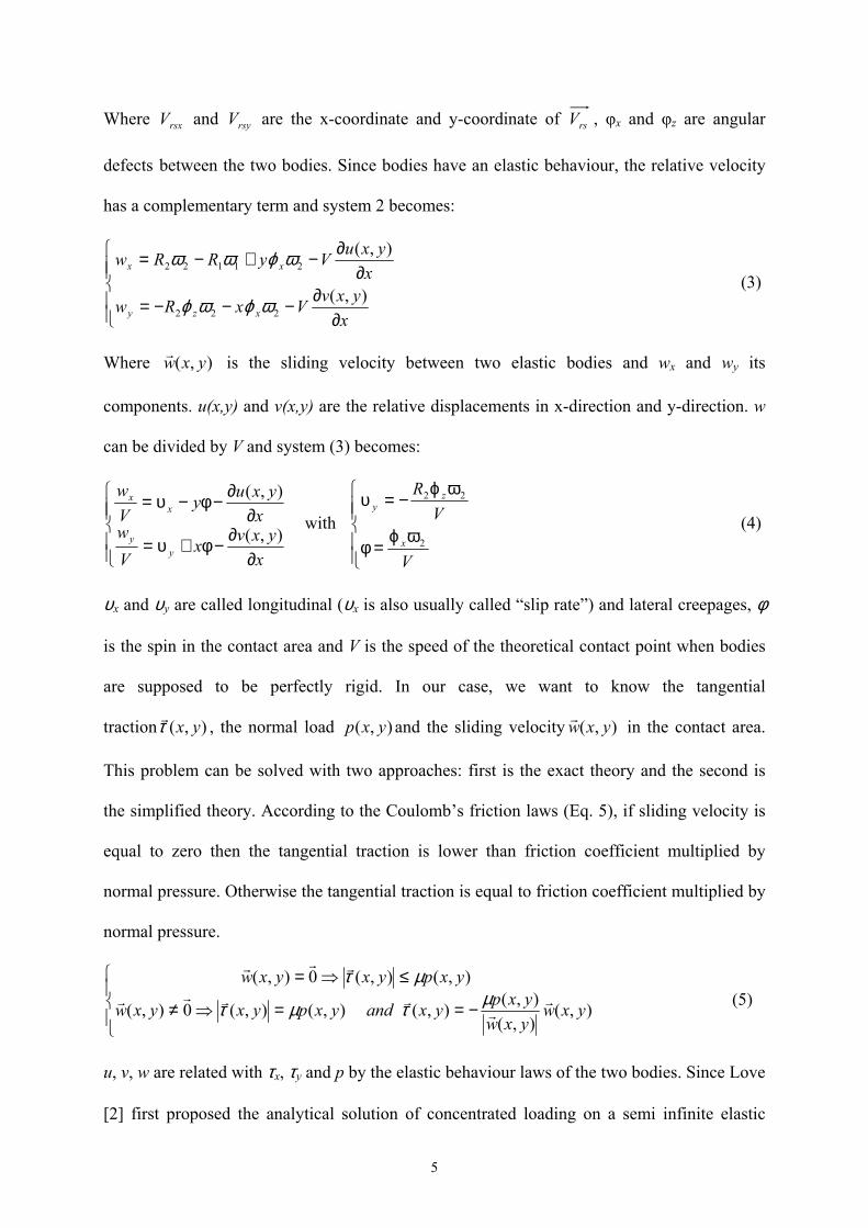
Where (x, y, z) are co-ordinates in x-direction, y-direction and z-direction of point M and (x’,
y’, z’) the co-ordinates of point M’ as presented in Fig 3.
The third relation of Eq.6, in the case of constant curvature in the contact area, is analogous to
the Hertz problem. Pressure distribution ),( yxp is elliptic, and contact area is an ellipse
where half lengths in both X and Y directions are denoted a and b and can be solved
separately from the first two relations in Eq. 6. The tangential problem is still coupled with
the normal problem by the friction law.
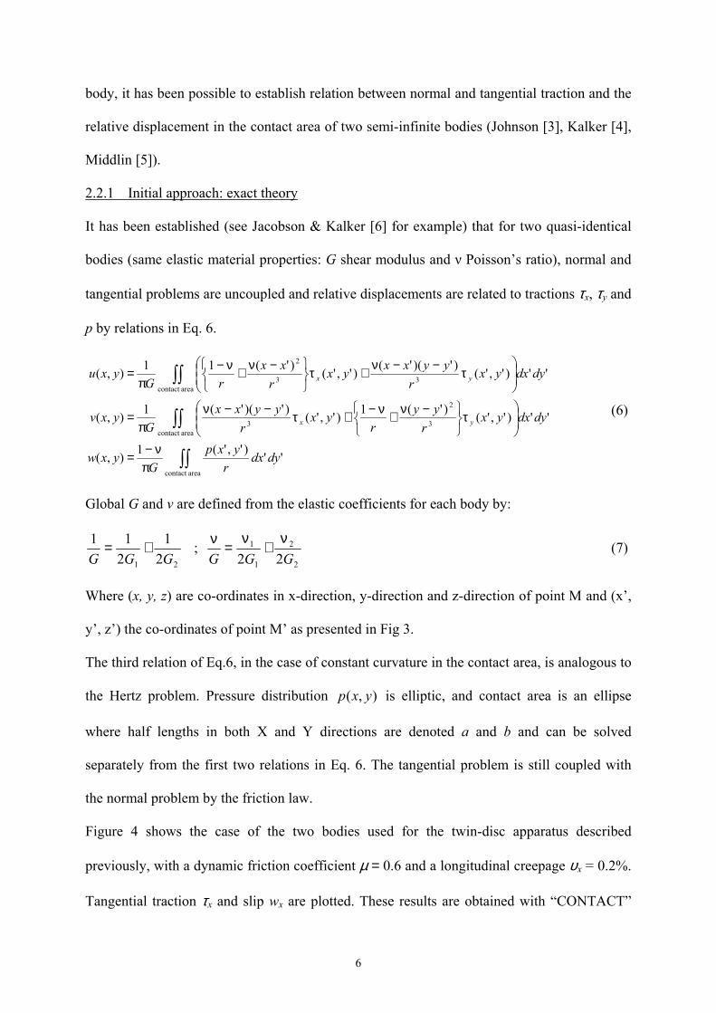
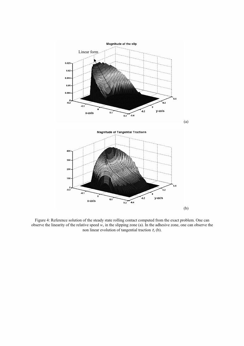
Figure 4 shows the case of the two bodies used for the twin-disc apparatus described
previously, with a dynamic friction coefficient µ = 0.6 and a longitudinal creepage υx = 0.2%.
Tangential traction τx and slip wx are plotted. These results are obtained with “CONTACT”
7
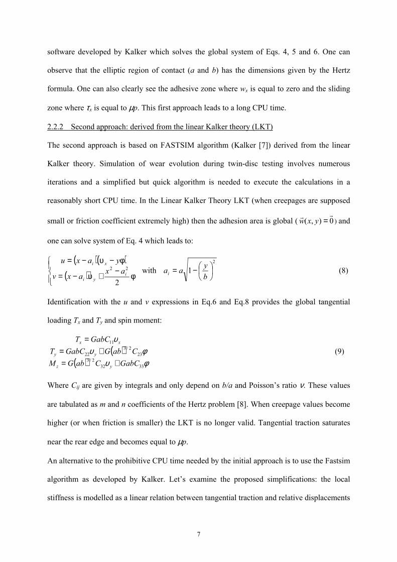
software developed by Kalker which solves the global system of Eqs. 4, 5 and 6. One can
observe that the elliptic region of contact (a and b) has the dimensions given by the Hertz
formula. One can also clearly see the adhesive zone where wx is equal to zero and the sliding
zone where τx is equal to µp. This first approach leads to a long CPU time.
2.2.2 Second approach: derived from the linear Kalker theory (LKT)
The second approach is based on FASTSIM algorithm (Kalker [7]) derived from the linear
Kalker theory. Simulation of wear evolution during twin-disc testing involves numerous
iterations and a simplified but quick algorithm is needed to execute the calculations in a
reasonably short CPU time. In the Linear Kalker Theory LKT (when creepages are supposed
small or friction coefficient extremely high) then the adhesion area is global ( 0),(rr =yxw ) and
one can solve system of Eq. 4 which leads to:
( )( )( )
φ−
+υ−=
φ−υ−=
2
22i
yi
xi
axaxv
yaxu
with 2
1
−=b
yaai (8)
Identification with the u and v expressions in Eq.6 and Eq.8 provides the global tangential
loading Tx and Ty and spin moment:
( )( ) φυ
φυυ
3332
2/323
2/3
22
11
GabCCabGM
CabGGabCT
GabCT
yz
yy
xx
+=+=
= (9)
Where Cij are given by integrals and only depend on b/a and Poisson’s ratio ν. These values
are tabulated as m and n coefficients of the Hertz problem [8]. When creepage values become
higher (or when friction is smaller) the LKT is no longer valid. Tangential traction saturates
near the rear edge and becomes equal to µp.
An alternative to the prohibitive CPU time needed by the initial approach is to use the Fastsim
algorithm as developed by Kalker. Let’s examine the proposed simplifications: the local
stiffness is modelled as a linear relation between tangential traction and relative displacements
8
u and v (i.e. u = L.τx. and v = L. τy). The L value depends of Cij coefficient, shear elastic
modulus G and ellipse dimensions a and b, but we must introduce three values to ensure that
the Tx and Ty components of LKT are identical in the case of global adhesion:
GC
baa
LGC
aL
GC
aL
23
3
22
2
11
14
,3
8,
3
8 π=== (10)
The simplified problem to solve is expressed by the relations of Eq.11. It is easy to see that
for an elliptic pressure distribution, the slip component will lead to infinity at the rear edge of
the contact. This is in contradiction with Fig. 4 and one can solve this problem using a
parabolic pressure distribution. This is an approximation that increases the maximum pressure
Po for 25% but gives good agreement in the tangential problem case.
∂∂
−+=
∂∂−−=
xL
x
LVL
w
xL
y
LVL
w
yyy
xxx
τφυ
τφυ
32
31 (11)
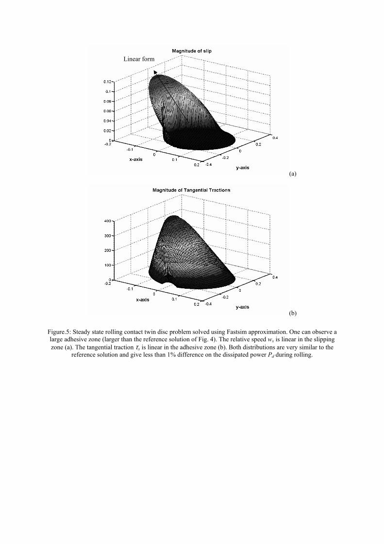
Solving the system in Eq. 11 leads to an analytical solution when spin is neglected. In the case
of µ = 0.6 and υx = 0.2 %, the solution is plotted in Fig. 5. We have compared the two
approaches in Fig. 4 and Fig. 5 and accuracy of the Fastsim solution is satisfactory.
Consequently we will solve the Fastsim approximation instead of the exact system in what
follows.
2.3. Dynamic friction coefficient identification
It has been shown in the previous section that when longitudinal creepage is sufficiently small
tangential traction τx is not equal to µp over the whole contact area. Consequently, summing
τx on this area gives a tangential global load T in the X direction which is lower than µN: the
ratio T/N is an apparent friction coefficient denoted µa. Figure 6 shows this apparent dynamic
friction coefficient versus longitudinal creepage for a µ value set to 0.6. One can see that
9
sliding becomes complete over the contact area for longitudinal creepage higher than 1%.
Even if the apparent friction coefficient gives a close approximation, one can see that it does
not superpose the measured points. This means that the real dynamic friction coefficient
varies for small values of creepage.
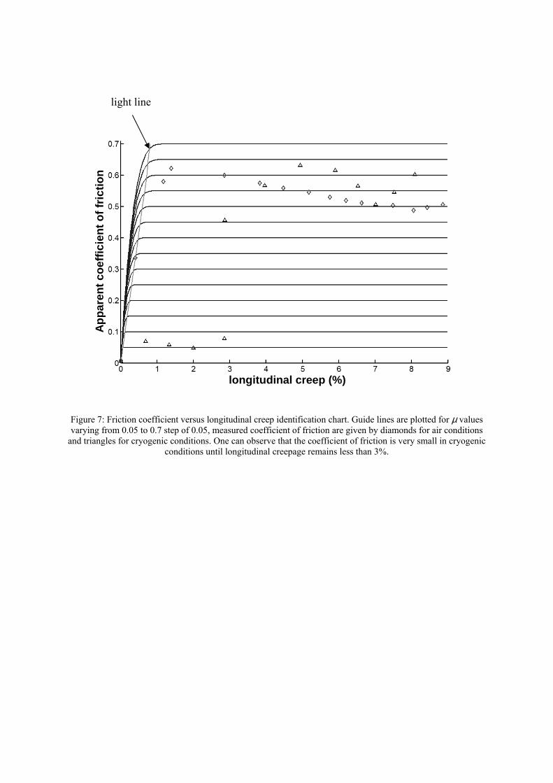
To conduct dynamic friction coefficient identification we propose the chart in Fig.7. Each
curve is obtained for a constant dynamic friction coefficient µ varying from 0.05 to 0.7. The
light line separates the small creepage values where an adhesive zone remains (local stick
area) on the contact area (in this case the slip is not global), and the higher values of υx where
sliding is complete on the contact area and the apparent dynamic friction coefficient is over
98% of the real value. The light line is obtained by plotting each point where µa equals 98 %
of µ.
One can see that experimental data always appear on the saturated zone of the apparent
dynamic friction coefficient excepted for the very first point in ambient air conditions. In case
of cryogenic condition, friction coefficient value is smaller and saturation appears for very
small values of longitudinal creepage. In both cases, this means that the sliding area appears
to be the total elliptic area of the contact zone for the measured points. Apparent dynamic
friction coefficient given by T/N is in fact, the real dynamic coefficient of friction. To
summarise our conclusions, the foregoing measurements have shown that:
(i) The dynamic friction coefficient depends on the longitudinal creepage value.
For very small values, friction is an increasing function of creepage. This
observation may appear to be a strange remark since it is classically admitted
that the adhesive friction coefficient is higher than the sliding dynamic
coefficient of friction. The steady state rolling calculation cannot provide the
static solution so we shall not further discuss on this first remark.
10
(ii) For high creepage values the dynamic friction coefficient is quite constant
(from 0.55 to 0.62 at ambient temperature and from 0.05 to 0.07 under Liquid
Nitrogen).
(iii) Cooling the rolling contact with Liquid Nitrogen reduces significantly the
sliding dynamic friction coefficient (about 10 times) but when sliding becomes
greater (about υx = 5%) the reducing effect of Liquid Nitrogen on the friction
coefficient vanishes.
This last remark requires a additional comment. The test has been repeated many times and
this “instability” of the friction coefficient always appears more or less at the same creepage
value. Some thermal effect may be in competition with the liquid nitrogen cooling . If one
could be able to quantify dissipated energy during the test it might be possible to quantify the
associated rise of temperature . This is point is developed in the final section.
The stick–slip partition of the contact area in steady state rolling has an impact on dissipated
power. Wear occurs and contact profiles fluctuate during the test. In the next section, we will
present the updating of the solid curvatures during the twin-disc test and will simulate both
wear evolution and temperature increase to conclude on the “instability” presented above. The
method used for wear simulation and other very similar methods have already been presented
in the literature (see [9], [10], [11] for example).
3. Wear simulation analysis
3.1 Loading history and wear measurement
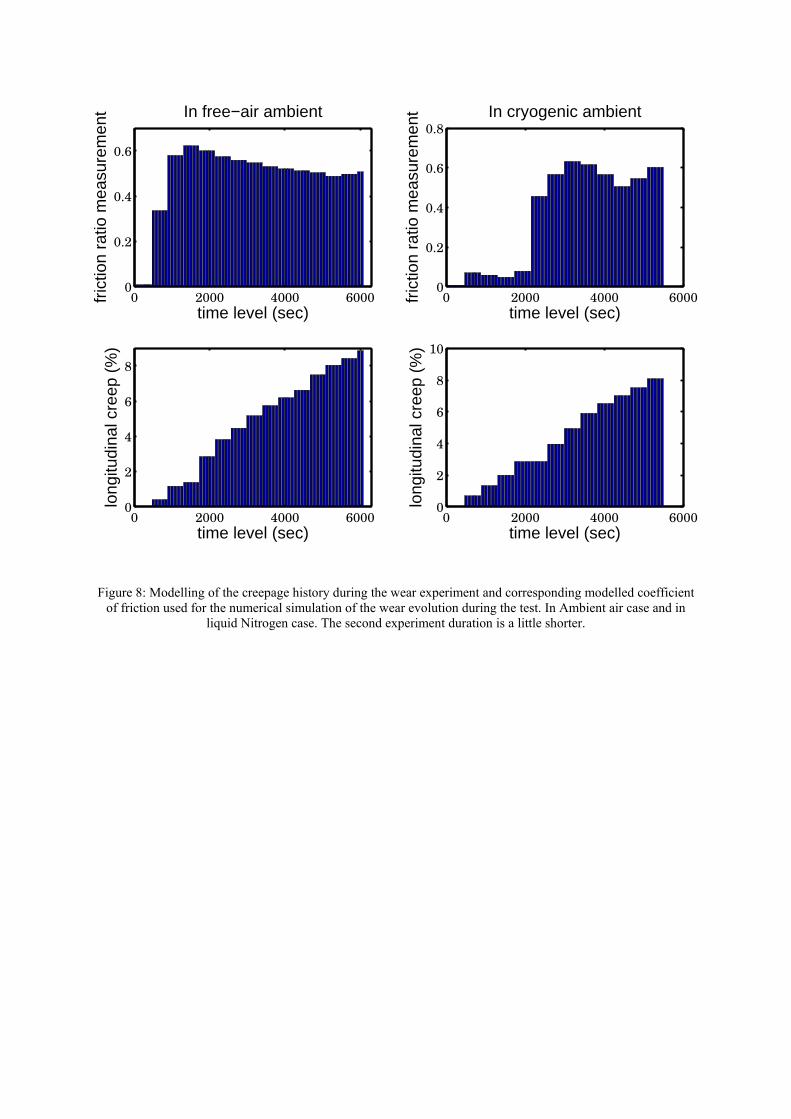
During the twin-disc experiment, a constant normal load N (N = 72 N) is applied but
longitudinal creepage υx and the friction coefficient vary following steps shown on Fig. 8 for
the two environments. Each step of υx is imposed for 5 iterations except the two last steps for
ambient air. One iteration corresponds to 4200 revolutions of each disc. These diagrams
11
present the paths followed in friction coefficient and in longitudinal creepage during
simulations in ambient cryogenic and ambient air. In the previous section we identified a
friction coefficient value µ for each one of these steps. Because friction coefficient µ and
longitudinal creepage υx influence dissipated power in the contact surface, they are factors
governing wear evolution. It is not surprising to observe that the rolling zone of the discs was
modified by the experiment.
Figure 9 shows the profile measured after the experiment for the two environments. One can
observe that both depth and width of the wear profile are smaller for ambient cryogenic than
for ambient air condition. This is logical if we consider that the dynamic friction coefficient is
lower for a considerable duration of the experiment. Nevertheless, the magnitudes of wear
depth fall within the same range of values (6 µm instead of 4.4 µm with liquid nitrogen) and
the width wear profile are smaller in ambient cryogenic than in ambient air (15.1 mm against
18 mm). The values of υx over 3% greatly effects the wear process. In order to compare both
wear evolutions, we performed numerical simulation of the wear process. At each step of the
simulation the increase of temperature has been evaluated.
3.2 Updated Hertzian approach for wear simulation
A model for material loss due to the cyclic rolling contact loading is provided by Archard’s
law [12]. A similar form was proposed by Zi Li & Kalker [11] and the mathematical
expression is given by Eq.12.
TLH
KW = (12)
W (m3) is the volume of wear, L (m) is the sliding length of the abrasive particle, T (N) is the
tangential load and H (N/m2) is the material hardness. Micro-hardness have been done and H
= 700 Hv. In Eq.12, K is a dimensionless coefficient characteristic of the materials in contact.
Simple microscopic interpretation of the “Archard’s factor” K is frequently given (see Felder
12
[13] or François & al. [14] for example) which suggests a relation between the factor K and
the dynamic friction coefficient µ. In that way, a low dynamic friction coefficient leads to
very small wear because of slight dissipated power during slip coupled with a small wear
factor. We will test this assumption in the following.
Tangential dissipated work is calculated by the product T times L. In an instantaneous form of
this model, the wear rate (m3/s) is directly proportional to the dissipated power Pd as defined
in Eq.13.
dPH
KW =& (13)
Pd is not uniformly distributed over the contact area and it is necessary to calculate the
tangential surface-traction distribution τ and the sliding velocity wg at each point on the
contact area to specify the distribution of dissipated energy per unit surface. We define the
wear depth rate u& (m/s) by Eq.14.
g
dW Ku w
dS Hτ= =
&& (14)
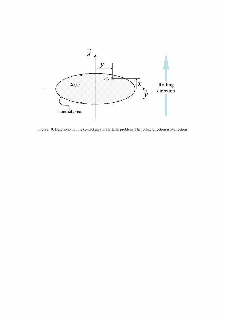
During a single pass of the roller on the cam track, the increment of the wear depth is obtained
by an integration over the time (t) of the wear depth rate from zero to ∆t = 2a(y)/V. Where V
is the rolling velocity and 2a(y) is the length of the contact stripe at abscise y as shown in Fig.
10. This yields to the incremental wear depth per roller passage δu/δn given by Eq.15 where
Pl(y) is the dissipated power per unit length.
)()(
yPHV
K
n
yul=
δδ
(15)
Pl(y) is calculated by integration over x (rolling direction) of tangential traction τ(x,y) times
sliding velocity w(x,y). Those quantities are inputs for the wear simulation software. For each
step of the simulation (one bar in the Fig.8 chart) wear is calculated from the dissipated power
per unit length with Eq.15. The best circle to fit the new profile is determined using a classical
13
least square distance method. Principal curvatures are updated and a new Fastsim calculation
is carried out. The evolution of wear profile can be estimated step by step.
3.3 Wear law identification
The wear factor K is unknown and must be identified from the experimental data. Different
methods (Newton-Raphson, Monte-Carlo ...) can be used to manage this identification. We
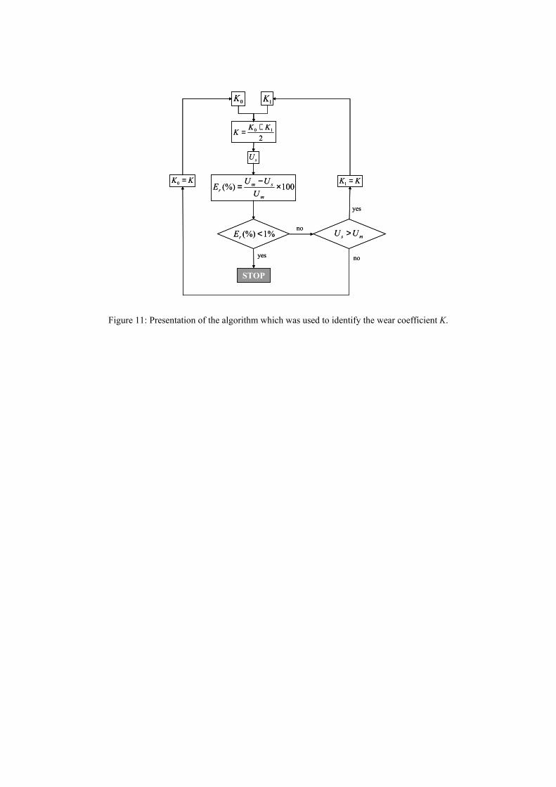
implement the following identification procedure by dichotomy:
(i) K0 and K1 values are chosen arbitrarily but these two values must include the solution
K. Then we define the solution K as it being the mean of K0 and K1.
210 KK
K+
= (16)
The principle of this method is to reduce the interval [K0 K1] to converge and to have
the solution K0 = K1 =K
(ii) The wear simulation is managed with the K value defined by Eq. 16 following the
conditions defined by Fig. 8. A wear profile )(yu s is obtained and we define Us as the
minimum of )(yu s . Us is compared to the minimum Um of wear measures.
(iii) An error Er(%) is defined by Eq. 17:
100(%) ×−
=m
smr
U
UUE (17)
(iv) If Er (%) < 1% then the calculation stops, otherwise
if Us > Um → the upper limit of the interval [K0 K1] was replaced by K: K1 = K
otherwise → the lower limit of the interval [K0 K1] was replaced by K: K0 = K
This procedure, summarised in Fig. 11, continues until the condition Er < 1% is satisfied.
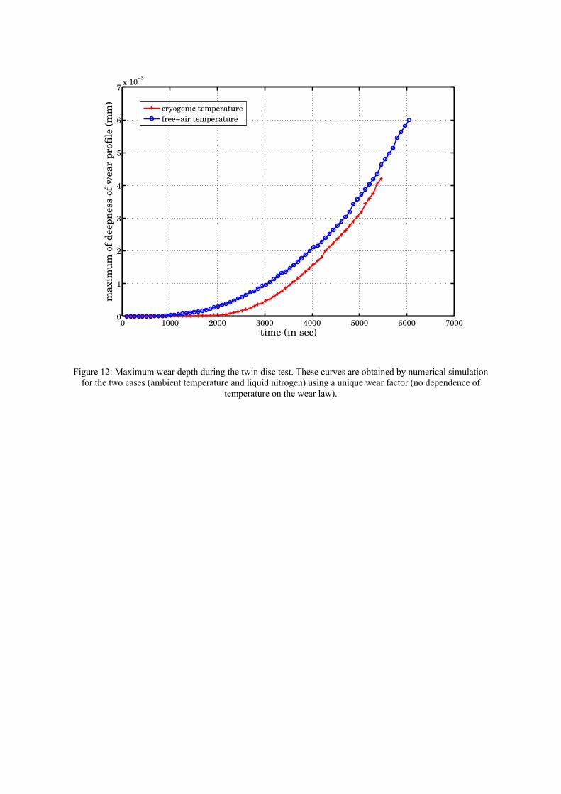
Using such a procedure for the ambient air case, we have identified the K value of 9.89.10-4.
Wear simulation in ambient cryogenic is then carried out. Figure 12 shows the maximum
depth of cryogenic conditions is accurately modelled with the same K value. This result is
14
important because it shows that the wear process is not influenced by the temperature and
only depends on the two materials. We believe that this conclusion must be accepted with
caution. We have here an identification obtained from on a global process where large
differences occur between the friction coefficient at the beginning of the Liquid Nitrogen test
(about 0.05) and the second part of the test where the friction coefficient rises up to 0.5.
Figure 12 shows that the wear evolution really begins after 2000 sec., which is the moment
where the friction coefficient increases and becomes equal to the one measured in ambient air
condition. This rise in the friction coefficient in cryogenic conditions may be due to an
increase in temperature at the contact point. Therefor then is a need to model the thermal
evolution originating from the dissipated power during rolling.
Assuming that the thermal problem is axisymetric and that the temperature is constant over
the thickness of the disc, the temperature is only a function of the radius r and time t The heat
transfer equation yields to Eq.18.
[ ])(1)(
∞−−=∆
∆TTShP
Cvt
tTwcd λ
ρ (18)
T is the mean temperature inside the disc at time t, Tw is the wall temperature on the external
radius of the disc r=R and ∞T is the temperature of the external ambient. C is the heat
capacity, v is the volume of disc, ρ is the disc density, S is the exchange surface, λ is the
thermal conductivity and hc is the forced convection exchange coefficient.
In order to estimate the contact temperature during the twin-disc test, we assume thatT has
the same order as wT . Eq. 18 can then be solved step by step and yields Eq. 19.
[ ])( 11 ∞++ −−∆+= TTShPCv
tTT icdii λ
ρ (19)
Ti+1 is computed at each time step i. ∞T will be set to the room temperature for the ambient air
test or to –196°C for the cryogenic condition. This calculation of the temperature evolution
15
necessitates a previous calculation of the power dissipated by rolling at each step of the
iterative numerical simulation managed to compute wear evolution.
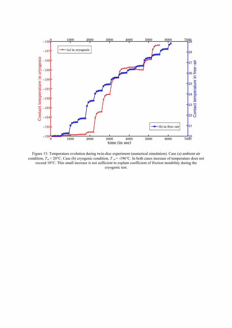
The temperature evolution for ambient conditions or cryogenic conditions is given on Fig.13.
It appears that the temperature increase during the ambient air test is about 10 °C. One can
note that the increase in temperature is nearly the same value as for the cryogenic conditions
and cannot explain the instability in the friction coefficient chart. We can observe a fall of
temperature near 4500 sec. in Fig. 13-b. This fall due to the decrease of the friction coefficient
imposed (Fig.8) in cryogenic conditions, and thus this can be explained by the low value of
dissipated power in regard of a small temperature growth.
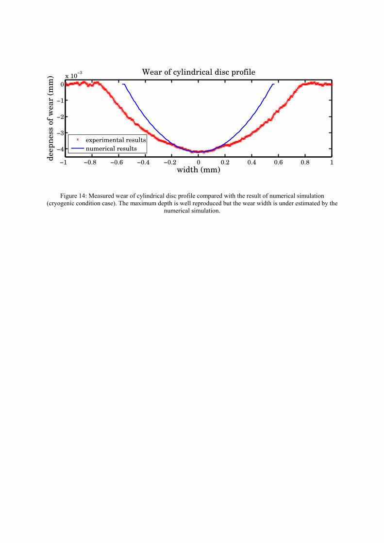
Figure 14 shows that the wear profile obtained by numerical simulation compares favourably
the depth of the measured wear profile of the cryogenic test. This is already a good point
because the wear factor has been identified from the ambient air test. One can observe that the
wear width is too small compared to the measured profile. This is certainly the consequence
of the procedure used to update curvatures at each step of the simulation and can be improved
by using a non linear wear law or by developing a semi-hertzian procedure as proposed by Zi
Li & Kalker [15] or by Ayasse & Chollet [16].
4. Conclusions
Experimental data obtained during twin-disc tests managed under ambient air and cryogenic
conditions have been analysed using a simplified modelling of steady state rolling. This
analysis enables accurate identification of slip influence on the friction ratio between discs.
The influence of temperature conditions has also been discussed and it appears that the
cooling contact yields to a spectacular decrease of the friction ratio compared to ambient
temperature conditions. Unfortunately, this low value is not stable and for 5% relative slip, the
friction coefficient rises to the nearly same value than at ambient temperature. It has been
16
shown that dissipation is not responsible for this instability, and at this time there is no
explanation for its existence.
Further investigation of the wear evolution that occurs during the test has been provided using
a classical Archard model. It appears that using the same wear factor at ambient air or
cryogenic conditions enables an accurate prediction of the wear profile depth at the end of the
test. Nevertheless, a semi Herztian approach must be implemented to be able to predict also
the wear profile width.
Nomenclature
a,b half length of elliptical surface (m) a(y) half length of contact band (m) Cij Kalker coefficients for elliptical contact C heat capacity E Young modulus (Pa) Er Error between Us et Um (%) G shear elastic modulus (Pa) or modulus of rigidity H material hardness (N/m²) hc forced convection exchange coefficient K non-dimensional coefficient that characterized a couple of materials: wear coefficient Lij value which depends of Cij Mz spin momentum around z-direction N normal load (N) n number of roller passage Po Hertz pressure (Pa) Pd dissipated power (W) Pl dissipated power per unit length (W/m) p(x,y) pressure distribution (Pa) L sliding length of the abrasive particle (m) Ri radius of disc i (m) Rb radius of spherical disc (m) T tangential load (N) Tx tangential load in x-direction Ty tangential load in y-direction
∞T temperature of the external ambient
Tw wall temperature on the external radius of the disc u& wear depth rate (m/s) u deepness of wear (m) ur displacement field : [ ]),(),,(),,( yxwyxvyxuu =r
Us minimum wear profile simulation us(y) (m) Um minimum of wear measure (m) V rolling velocity (m/s) Vd Volume of disc (m3) Vmean mean of rolling velocity (m/s)
rsV rigid sliding velocity (m/s)
Vrsx, Vrsy x-coordinate and y-coordinate of the rigid sliding velocity (m/s) W volume of wear (m3)
W& wear rate (m3/s)
17
w(x,y) sliding velocity (m/s) wx sliding velocity in x-direction (m/s) wy sliding velocity in y-direction (m/s) Greek letters
λ thermal conductivity µ friction coefficient µa apparent friction coefficient ν Poisson’s ratio υx longitudinal creep coefficient υy transversal creep coefficient τ(x,y) tangential traction (Pa) τx tangential traction in x-direction (Pa) τy tangential traction in y-direction (Pa) φ spin in the contact area (m-1) φx, φy angular defect of positioning body (rad) ωi rotating velocity (rad/s) of disc i
List of figures
Figure 1: Twin-disc apparatus. Rotation rates are imposed to both discs and slip can be controlled. Normal load N between the two discs is constant during the test and tangential load T is measured continuously. Rotation rate is about 3000 rpm. The velocity of the contact point is about 9.5 m/s.
Figure 2: Longitudinal creep (slip rate) and traction coefficient T/N versus time respectively imposed and measured during the twin disc experimentation in ambient air and in cryogenic ambient Figure 3: Potential contact area considered to solve the exact problem. d(MM’) is the relative displacement between two points M and M’.
Figure 4: Reference solution of the steady state rolling contact computed from the exact problem. One can observe the linearity of the relative speed wx in the slipping zone (a). In the adhesive zone, one can observe the non linear evolution of tangential traction τx (b).
Figure 5: Steady state rolling contact twin disc problem solved using Fastsim approximation. One can observe a large adhesive zone (larger than the reference solution of Fig. 4). The relative speed wx is linear in the slipping zone (a). The tangential traction τx is linear in the adhesive zone (b). Both distributions are very similar to the reference solution and give less than 1% difference on the dissipated power Pd during rolling.
Figure 6: Apparent coefficient of friction µa versus longitudinal creep for µ = 0.6. Experimental values of ambient air test are superposed (diamonds) and follow approximately the same evolution. The partition between slipping zone and adhesive zone is illustrated for several longitudinal creepage values. When slip occurs on the complete contact area the apparent coefficient of friction µa is equal to the real coefficient of friction µ.
Figure 7: Friction coefficient versus longitudinal creep identification chart. Guide lines are plotted for µ values varying from 0.05 to 0.7 step of 0.05, measured coefficient of friction are given by diamonds for air conditions and triangles for cryogenic conditions. One can observe that the coefficient of friction is very small in cryogenic conditions until longitudinal creepage remains less than 3%.
Figure 8: Modelling of the creepage history during the wear experiment and corresponding modelled coefficient of friction used for the numerical simulation of the wear evolution during the test. In Ambient air case and in liquid Nitrogen case. The second experiment duration is a little shorter.
Figure 9: Rolling zone profile for disc 1 after the experiment for N = 72N in ambient air (top) and in Liquid nitrogen condition (bottom). One can see that wear depth is lower for cryogenic condition than for ambient air condition, which is easily justified by the lower value of the mean friction ratio during the test and the smaller duration of the same test.
Figure 10: Description of the contact area in Hertzian problem. The rolling direction is in x-direction
Figure 11: Presentation of the algorithm which was used to identify the wear coefficient K
18
Figure 12: Maximum wear depth during the twin disc test. These curves are obtained by numerical simulation for the two cases (ambient temperature and liquid nitrogen) using a unique wear factor (no dependence of temperature on the wear law).
Figure 13: Temperature evolution during twin-disc experiment (numerical simulation). Case (a) ambient air condition, T∞ = 20°C. Case (b) cryogenic condition, T ∞
= -196°C. In both cases increase of temperature does not exceed 10°C. This small increase is not sufficient to explain friction ratio instability during the cryogenic test.
Figure 14: Measured wear of cylindrical disc profile compared with the result of numerical simulation (cryogenic condition case). The maximum depth is well reproduced but the wear width is under estimated by the numerical simulation.
References
[1] M. Quillien, R. Gras, L. Collongeat, Th. Kachler, ‘A testing device for rolling-sliding behavior in harsh environments : the twin-disk cryotribometer’ Trib. Int. 34 (2001) 287-292 [2] A.E.H. Love, ‘A treatise on the theory of elasticity’, 4th Ed. Cambridge University press (1926) [3] K.L. Johnson, ‘Contact Mechanics’, Cambridge University Press (1985) [4] J. J. Kalker, ‘Three-Dimensional Elastic Bodies in Rolling Contact’, Kluwer Academic (1991) [5] R.D. Mindlin, ‘Compliance of elastic bodies in contact’,ASME J. Appl. Mech. (1949), 259-268 [6] B. Jacobson, J.J. Kalker, ‘Rolling Contact Phenomena’, CISM Lecture No. 411, Springer, Berlin (2000). [7] J. J. Kalker, ‘A Fast Algorithm for the Simplified Theory of Rolling Contact’, (program FASTSIM), Vehicle Systems Dynamics, Vol. 11 pp 1-13, SWETS & ZEITLINGER B.V. - LISSE, (1982) [8] H. Hertz, ‘Über die berührung fester elasticher körper (on the contact of elastic solids)’, J. Reine und Angewandte Mathematik 92, (1882) 156-171, translated and reprinted in Hertz’s Miscelaneous Papers, MacMillan & Co, London, (1896). [9] L.Chevalier et H.Chollet, ‘Endommagement des pistes de roulement’, Mec. Ind.(2000) 1, 593-602 [10] W.Kik, J.Piotrowski, 'A fast approximate method to calculate normal load at contact between wheel and rail, and creep forces during rolling', Warsaw Technical University, 2nd mini-conference on contact mechanics and wear of rail/wheel systems, Budapest, July 29-31 (1996) [11] Zi-Li Li, Kalker J.J., ‘Simulation of Severe Wheel-Rail Wear’, Delft University 1996 [12] J.F. Archard, ‘Contact and rubbing of flat surfaces’, J.Appl. Phys. 24 (1953), 981-988 [13] E.Felder, ‘Mécanismes physiques et modélisation mécanique du frottement entre corps solides’, Mec. Ind. 1 2 (2000) 555-561 [14] D.François, A.Pineau, A.Zaoui, ‘Comportement mécanique des matériaux, tome 2’, Hermès (1993), 401-450 159-166 [15] Z.L.Li, J.J.Kalker, ‘Computation of wheel-rail conformal contact’, Proc. of 4th world cong. on computational mechanics, BuenosAires, (July 1998) [16] Ayasse J.B., Chollet H., ‘Determination of the wheel rail contact patch in semi-Hertzian conditions, Vehicle Systems Dynamics, 43, 3 (2005) 161-172
ω1
R2
R1
Brushless
Motor 1
Spindles
DiscsCryostat
Load
kg
Belt
Rb
Brushless
Motor 2
ω2
ω2ω1
ω1
R2
R1
Brushless
Motor 1
SpindlesSpindles
DiscsDiscsCryostatCryostat
Load
kg
Belt
Rb
Brushless
Motor 2
ω2
ω2ω1
Figure 1: Twin-disc apparatus. Rotation rates are imposed to both discs and slip can be controlled. Normal load N between the two discs is constant during the test and tangential load T is measured continuously. Rotation rate
is about 3000 rpm. The rolling velocity of the contact point is about 9.5 m/s.
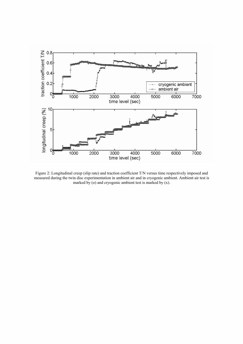
Figure 2: Longitudinal creep (slip rate) and traction coefficient T/N versus time respectively imposed and measured during the twin disc experimentation in ambient air and in cryogenic ambient. Ambient air test is
marked by (o) and cryogenic ambient test is marked by (x).

X
Y
M
M’
d(MM’)
Aire potentielle de contact
Élément desurface dS(M’)Elementary area dS (M’)
Potential contact area
X
Y
M
M’
d(MM’)
Aire potentielle de contact
Élément desurface dS(M’)Elementary area dS (M’)
Potential contact area
Figure 3: Potential contact area considered to solve the exact problem. The distance d(MM’) between two points
M and M’ is noted ‘r’ in the text: d(MM’) = 22 )'()'( yyxxr −+−= .
(a)
(b)
Figure 4: Reference solution of the steady state rolling contact computed from the exact problem. One can observe the linearity of the relative speed wx in the slipping zone (a). In the adhesive zone, one can observe the
non linear evolution of tangential traction τx (b).
Linear form
(a)
(b)
Figure.5: Steady state rolling contact twin disc problem solved using Fastsim approximation. One can observe a large adhesive zone (larger than the reference solution of Fig. 4). The relative speed wx is linear in the slipping zone (a). The tangential traction τx is linear in the adhesive zone (b). Both distributions are very similar to the
reference solution and give less than 1% difference on the dissipated power Pd during rolling.
Linear form
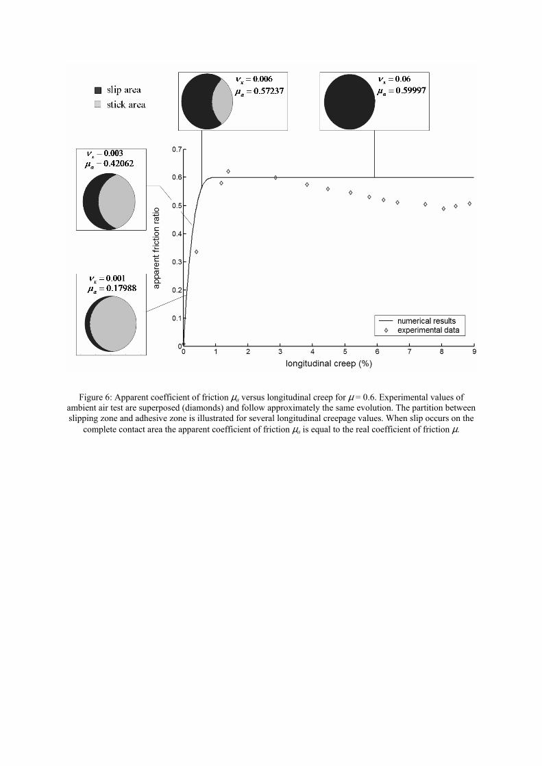
Figure 6: Apparent coefficient of friction µa versus longitudinal creep for µ = 0.6. Experimental values of ambient air test are superposed (diamonds) and follow approximately the same evolution. The partition between slipping zone and adhesive zone is illustrated for several longitudinal creepage values. When slip occurs on the
complete contact area the apparent coefficient of friction µa is equal to the real coefficient of friction µ.
longitudinal creep (%)
Ap
par
ent
coef
fici
ent
of
fric
tio
n
longitudinal creep (%)
Ap
par
ent
coef
fici
ent
of
fric
tio
n
Figure 7: Friction coefficient versus longitudinal creep identification chart. Guide lines are plotted for µ values varying from 0.05 to 0.7 step of 0.05, measured coefficient of friction are given by diamonds for air conditions and triangles for cryogenic conditions. One can observe that the coefficient of friction is very small in cryogenic
conditions until longitudinal creepage remains less than 3%.
light line
0 2000 4000 60000
0.2
0.4
0.6
time level (sec)
fric
tion
ratio
mea
sure
men
t In free−air ambient
0 2000 4000 60000
2
4
6
8
time level (sec)
long
itudi
nal c
reep
(%
)
0 2000 4000 60000
0.2
0.4
0.6
0.8
time level (sec)
fric
tion
ratio
mea
sure
men
t In cryogenic ambient
0 2000 4000 60000
2
4
6
8
10
time level (sec)
long
itudi
nal c
reep
(%
)
Figure 8: Modelling of the creepage history during the wear experiment and corresponding modelled coefficient of friction used for the numerical simulation of the wear evolution during the test. In Ambient air case and in
liquid Nitrogen case. The second experiment duration is a little shorter.
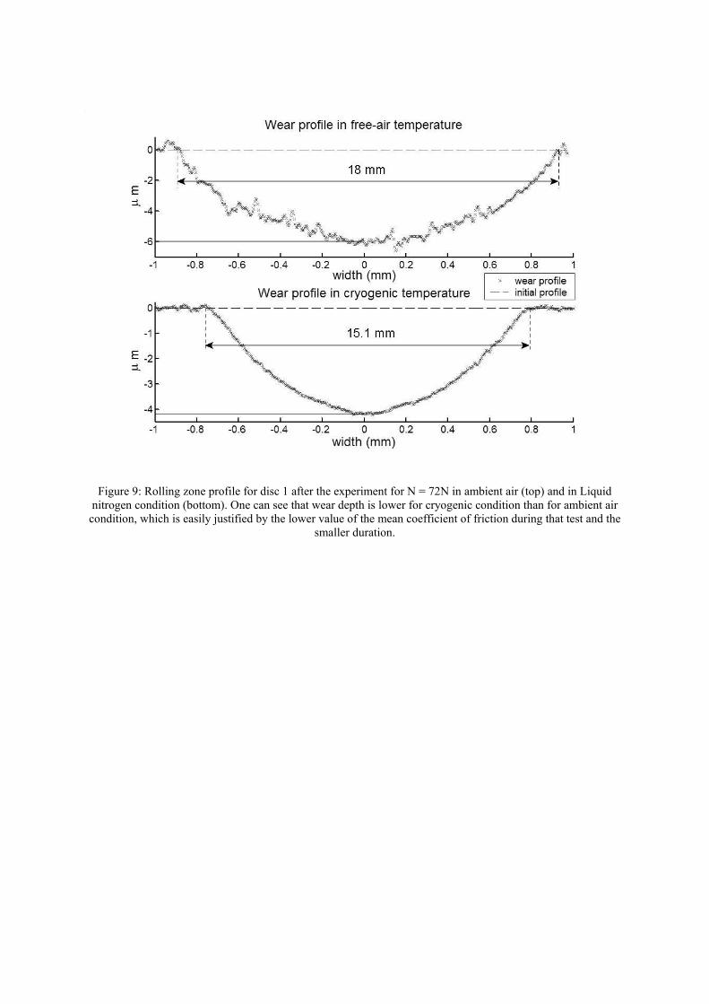
Figure 9: Rolling zone profile for disc 1 after the experiment for N = 72N in ambient air (top) and in Liquid nitrogen condition (bottom). One can see that wear depth is lower for cryogenic condition than for ambient air condition, which is easily justified by the lower value of the mean coefficient of friction during that test and the
smaller duration.
Rolling directionRolling directionRolling direction
Figure 10: Description of the contact area in Hertzian problem. The rolling direction is x-direction
0K 1K
210 KK
K+
=
sU
100(%) ×−
=m
sm
rU
UUE
%1(%) <rE
STOP
yes
noms UU >
KK =1KK =0
yes
no
0K 1K
210 KK
K+
=
sU
100(%) ×−
=m
sm
rU
UUE
%1(%) <rE
STOP
yes
noms UU >
KK =1KK =0
yes
no
Figure 11: Presentation of the algorithm which was used to identify the wear coefficient K.
0 1000 2000 3000 4000 5000 6000 70000
1
2
3
4
5
6
7x 10
−3
time (in sec)
maxim
um
of
deep
ness
of
wear
pro
file
(m
m)
cryogenic temperature
free−air temperature
Figure 12: Maximum wear depth during the twin disc test. These curves are obtained by numerical simulation for the two cases (ambient temperature and liquid nitrogen) using a unique wear factor (no dependence of
temperature on the wear law).
0 1000 2000 3000 4000 5000 6000 7000−196
−195
−194
−193
−192
−191
−190
−189
−188
−187
−186
time (in sec)
Con
tact
tem
pera
ture
in
cry
ogen
ic
(a) in cryogenic
0 1000 2000 3000 4000 5000 6000 7000
20
21
22
23
24
25
26
27
28
29
Con
tact
tem
pera
ture
in fr
ee−
air
(b) in free−air
Figure 13: Temperature evolution during twin-disc experiment (numerical simulation). Case (a) ambient air
condition, T∞ = 20°C. Case (b) cryogenic condition, T ∞ = -196°C. In both cases increase of temperature does not
exceed 10°C. This small increase is not sufficient to explain coefficient of friction instability during the cryogenic test.
−1 −0.8 −0.6 −0.4 −0.2 0 0.2 0.4 0.6 0.8 1
−4
−3
−2
−1
0
x 10−3
width (mm)
deep
ness
of
wea
r (m
m)
Wear of cylindrical disc profile
experimental results
numerical results
Figure 14: Measured wear of cylindrical disc profile compared with the result of numerical simulation (cryogenic condition case). The maximum depth is well reproduced but the wear width is under estimated by the
numerical simulation.