Embed Size (px)
Citation preview
Introduction
1 Introduction2 Combinatorial Methods
3 Binomial Coefficients4 The Theory in Practice
1 Introduction In recent years, the growth of statistics has made itself felt in almost every phaseof human activity. Statistics no longer consists merely of the collection of data andtheir presentation in charts and tables; it is now considered to encompass the scienceof basing inferences on observed data and the entire problem of making decisionsin the face of uncertainty. This covers considerable ground since uncertainties aremet when we flip a coin, when a dietician experiments with food additives, when anactuary determines life insurance premiums, when a quality control engineer acceptsor rejects manufactured products, when a teacher compares the abilities of students,when an economist forecasts trends, when a newspaper predicts an election, andeven when a physicist describes quantum mechanics.
It would be presumptuous to say that statistics, in its present state of devel-opment, can handle all situations involving uncertainties, but new techniques areconstantly being developed and modern statistics can, at least, provide the frame-work for looking at these situations in a logical and systematic fashion. In otherwords, statistics provides the models that are needed to study situations involvinguncertainties, in the same way as calculus provides the models that are needed todescribe, say, the concepts of Newtonian physics.
The beginnings of the mathematics of statistics may be found in mid-eighteenth-century studies in probability motivated by interest in games of chance. The theorythus developed for “heads or tails” or “red or black” soon found applications in sit-uations where the outcomes were “boy or girl,” “life or death,” or “pass or fail,” andscholars began to apply probability theory to actuarial problems and some aspectsof the social sciences. Later, probability and statistics were introduced into physicsby L. Boltzmann, J. Gibbs, and J. Maxwell, and by this century they have foundapplications in all phases of human endeavor that in some way involve an elementof uncertainty or risk. The names that are connected most prominently with thegrowth of mathematical statistics in the first half of the twentieth century are thoseof R. A. Fisher, J. Neyman, E. S. Pearson, and A. Wald. More recently, the work ofR. Schlaifer, L. J. Savage, and others has given impetus to statistical theories basedessentially on methods that date back to the eighteenth-century English clergymanThomas Bayes.
Mathematical statistics is a recognized branch of mathematics, and it can bestudied for its own sake by students of mathematics. Today, the theory of statistics isapplied to engineering, physics and astronomy, quality assurance and reliability, drugdevelopment, public health and medicine, the design of agricultural or industrialexperiments, experimental psychology, and so forth. Those wishing to participate
From Chapter 1 of John E. Freund’s Mathematical Statistics with Applications,Eighth Edition. Irwin Miller, Marylees Miller. Copyright 2014 by Pearson Education, Inc.All rights reserved.

Introduction
in such applications or to develop new applications will do well to understand themathematical theory of statistics. For only through such an understanding can appli-cations proceed without the serious mistakes that sometimes occur. The applicationsare illustrated by means of examples and a separate set of applied exercises, manyof them involving the use of computers. To this end, we have added at the end of thechapter a discussion of how the theory of the chapter can be applied in practice.
We begin with a brief review of combinatorial methods and binomialcoefficients.
2 Combinatorial Methods
In many problems of statistics we must list all the alternatives that are possible in agiven situation, or at least determine how many different possibilities there are. Inconnection with the latter, we often use the following theorem, sometimes called thebasic principle of counting, the counting rule for compound events, or the rule for
the multiplication of choices.
THEOREM 1. If an operation consists of two steps, of which the first can bedone in n1 ways and for each of these the second can be done in n2 ways,then the whole operation can be done in n1·n2 ways.
Here, “operation” stands for any kind of procedure, process, or method of selection.To justify this theorem, let us define the ordered pair (xi, yj) to be the outcome
that arises when the first step results in possibility xi and the second step results inpossibility yj. Then, the set of all possible outcomes is composed of the followingn1·n2 pairs:
(x1, y1), (x1, y2), . . . , (x1, yn2)
(x2, y1), (x2, y2), . . . , (x2, yn2)
. . .
. . .
. . .
(xn1 , y1), (xn1 , y2), . . . , (xn1 , yn2)
EXAMPLE 1
Suppose that someone wants to go by bus, train, or plane on a week’s vacation to oneof the five East North Central States. Find the number of different ways in which thiscan be done.
Solution
The particular state can be chosen in n1 = 5 ways and the means of transportationcan be chosen in n2 = 3 ways. Therefore, the trip can be carried out in 5 · 3 = 15possible ways. If an actual listing of all the possibilities is desirable, a tree diagram
like that in Figure 1 provides a systematic approach. This diagram shows that thereare n1 = 5 branches (possibilities) for the number of states, and for each of thesebranches there are n2 = 3 branches (possibilities) for the different means of trans-portation. It is apparent that the 15 possible ways of taking the vacation are repre-sented by the 15 distinct paths along the branches of the tree.
!

Introduction
bus
train
plane
Illinois
bus
train
plane
Ohio
India
na
Michigan
Wisco
nsin
bus
train
plane
bus
train
plane
bus
train
plane
Figure 1. Tree diagram.
EXAMPLE 2
How many possible outcomes are there when we roll a pair of dice, one red andone green?
Solution
The red die can land in any one of six ways, and for each of these six ways the greendie can also land in six ways. Therefore, the pair of dice can land in 6 · 6 = 36 ways.
Theorem 1 may be extended to cover situations where an operation consists oftwo or more steps. In this case, we have the following theorem.
"

Introduction
THEOREM 2. If an operation consists of k steps, of which the first can bedone in n1 ways, for each of these the second step can be done in n2 ways,for each of the first two the third step can be done in n3 ways, and so forth,then the whole operation can be done in n1 ·n2 · . . . ·nk ways.
EXAMPLE 3
A quality control inspector wishes to select a part for inspection from each of fourdifferent bins containing 4, 3, 5, and 4 parts, respectively. In how many different wayscan she choose the four parts?
Solution
The total number of ways is 4 · 3 · 5 · 4 = 240.
EXAMPLE 4
In how many different ways can one answer all the questions of a true–false testconsisting of 20 questions?
Solution
Altogether there are
2 · 2 · 2 · 2 · . . . · 2 · 2 = 220 = 1,048,576
different ways in which one can answer all the questions; only one of these corre-sponds to the case where all the questions are correct and only one corresponds tothe case where all the answers are wrong.
Frequently, we are interested in situations where the outcomes are the differentways in which a group of objects can be ordered or arranged. For instance, we mightwant to know in how many different ways the 24 members of a club can elect a presi-dent, a vice president, a treasurer, and a secretary, or we might want to know in howmany different ways six persons can be seated around a table. Different arrange-ments like these are called permutations.
DEFINITION 1. PERMUTATIONS. A permutation is a distinct arrangement of n differ-
ent elements of a set.
EXAMPLE 5
How many permutations are there of the letters a, b, and c?
Solution
The possible arrangements are abc, acb, bac, bca, cab, and cba, so the number ofdistinct permutations is six. Using Theorem 2, we could have arrived at this answerwithout actually listing the different permutations. Since there are three choices to
#

Introduction
select a letter for the first position, then two for the second position, leaving onlyone letter for the third position, the total number of permutations is 3 · 2 · 1 = 6.
Generalizing the argument used in the preceding example, we find that n distinctobjects can be arranged in n(n− 1)(n− 2) · . . . · 3 · 2 · 1 different ways. To simplify ournotation, we represent this product by the symbol n!, which is read “n factorial.”Thus, 1! = 1, 2! = 2 · 1 = 2, 3! = 3 · 2 · 1 = 6, 4! = 4 · 3 · 2 · 1 = 24, 5! = 5 · 4 · 3 · 2 · 1 =120, and so on. Also, by definition we let 0! = 1.
THEOREM 3. The number of permutations of n distinct objects is n!.
EXAMPLE 6
In how many different ways can the five starting players of a basketball team beintroduced to the public?
Solution
There are 5! = 5 · 4 · 3 · 2 · 1 = 120 ways in which they can be introduced.
EXAMPLE 7
The number of permutations of the four letters a, b, c, and d is 24, but what is thenumber of permutations if we take only two of the four letters or, as it is usually put,if we take the four letters two at a time?
Solution
We have two positions to fill, with four choices for the first and then three choices forthe second. Therefore, by Theorem 1, the number of permutations is 4 · 3 = 12.
Generalizing the argument that we used in the preceding example, we find that n
distinct objects taken r at a time, for r > 0, can be arranged in n(n− 1) · . . . ·(n− r+ 1) ways. We denote this product by nPr, and we let nP0 = 1 by definition.Therefore, we can state the following theorem.
THEOREM 4. The number of permutations of n distinct objects taken r at atime is
nPr =n!
(n− r)!
for r = 0, 1, 2, . . . , n.
Proof The formula nPr = n(n− 1) · . . . · (n− r+ 1) cannot be used forr = 0, but we do have
nP0 =n!
(n− 0)!= 1
$

Introduction
For r = 1, 2, . . . , n, we have
nPr = n(n− 1)(n− 2) · . . . · (n− r− 1)
=n(n− 1)(n− 2) · . . . · (n− r− 1)(n− r)!
(n− r)!
=n!
(n− r)!
In problems concerning permutations, it is usually easier to proceed by usingTheorem 2 as in Example 7, but the factorial formula of Theorem 4 is somewhateasier to remember. Many statistical software packages provide values of nPr andother combinatorial quantities upon simple commands. Indeed, these quantities arealso preprogrammed in many hand-held statistical (or scientific) calculators.
EXAMPLE 8
Four names are drawn from among the 24 members of a club for the offices of pres-ident, vice president, treasurer, and secretary. In how many different ways can thisbe done?
Solution
The number of permutations of 24 distinct objects taken four at a time is
24P4 =24!
20!= 24 · 23 · 22 · 21 = 255,024
EXAMPLE 9
In how many ways can a local chapter of the American Chemical Society schedulethree speakers for three different meetings if they are all available on any of fivepossible dates?
Solution
Since we must choose three of the five dates and the order in which they are chosen(assigned to the three speakers) matters, we get
5P3 =5!
2!=
120
2= 60
We might also argue that the first speaker can be scheduled in five ways, the sec-ond speaker in four ways, and the third speaker in three ways, so that the answer is5 · 4 · 3 = 60.
Permutations that occur when objects are arranged in a circle are calledcircular permutations. Two circular permutations are not considered different (andare counted only once) if corresponding objects in the two arrangements have thesame objects to their left and to their right. For example, if four persons are playingbridge, we do not get a different permutation if everyone moves to the chair at hisor her right.
%

Introduction
EXAMPLE 10
How many circular permutations are there of four persons playing bridge?
Solution
If we arbitrarily consider the position of one of the four players as fixed, we can seat(arrange) the other three players in 3! = 6 different ways. In other words, there aresix different circular permutations.
Generalizing the argument used in the preceding example, we obtain the follow-ing theorem.
THEOREM 5. The number of permutations of n distinct objects arranged ina circle is (n− 1)!.
We have been assuming until now that the n objects from which we select r
objects and form permutations are all distinct. Thus, the various formulas cannot beused, for example, to determine the number of ways in which we can arrange theletters in the word “book,” or the number of ways in which three copies of one noveland one copy each of four other novels can be arranged on a shelf.
EXAMPLE 11
How many different permutations are there of the letters in the word “book”?
Solution
If we distinguish for the moment between the two o’s by labeling them o1 and o2,there are 4! = 24 different permutations of the symbols b, o1, o2, and k. However, ifwe drop the subscripts, then bo1ko2 and bo2ko1, for instance, both yield boko, andsince each pair of permutations with subscripts yields but one arrangement withoutsubscripts, the total number of arrangements of the letters in the word “book” is242 = 12.
EXAMPLE 12
In how many different ways can three copies of one novel and one copy each of fourother novels be arranged on a shelf?
Solution
If we denote the three copies of the first novel by a1, a2, and a3 and the other fournovels by b, c, d, and e, we find that with subscripts there are 7! different permuta-tions of a1, a2, a3, b, c, d, and e. However, since there are 3! permutations of a1, a2,and a3 that lead to the same permutation of a, a, a, b, c, d, and e, we find that thereare only 7!
3! = 7 · 6 · 5 · 4 = 840 ways in which the seven books can be arranged on ashelf.
Generalizing the argument that we used in the two preceding examples, weobtain the following theorem.
&

Introduction
THEOREM 6. The number of permutations of n objects of which n1 are ofone kind, n2 are of a second kind, . . . , nk are of a kth kind, andn1+n2+ · · ·+nk = n is
n!
n1! ·n2! · . . . ·nk!
EXAMPLE 13
In how many ways can two paintings by Monet, three paintings by Renoir, and twopaintings by Degas be hung side by side on a museum wall if we do not distinguishbetween the paintings by the same artists?
Solution
Substituting n = 7, n1 = 2, n2 = 3, and n3 = 2 into the formula of Theorem 6, we get
7!
2! · 3! · 2!= 210
There are many problems in which we are interested in determining the numberof ways in which r objects can be selected from among n distinct objects without
regard to the order in which they are selected.
DEFINITION 2. COMBINATIONS. A combination is a selection of r objects taken from
n distinct objects without regard to the order of selection.
EXAMPLE 14
In how many different ways can a person gathering data for a market research orga-nization select three of the 20 households living in a certain apartment complex?
Solution
If we care about the order in which the households are selected, the answer is
20P3 = 20 · 19 · 18 = 6,840
but each set of three households would then be counted 3! = 6 times. If we do notcare about the order in which the households are selected, there are only6,840
6= 1,140 ways in which the person gathering the data can do his or her job.
Actually, “combination” means the same as “subset,” and when we ask for thenumber of combinations of r objects selected from a set of n distinct objects, we aresimply asking for the total number of subsets of r objects that can be selected froma set of n distinct objects. In general, there are r! permutations of the objects in asubset of r objects, so that the nPr permutations of r objects selected from a set ofn distinct objects contain each subset r! times. Dividing nPr by r! and denoting the
result by the symbol(
nr
)
, we thus have the following theorem.
'

Introduction
THEOREM 7. The number of combinations of n distinct objects taken r at atime is
(
n
r
)
=n!
r!(n− r)!
for r = 0, 1, 2, . . . , n.
EXAMPLE 15
In how many different ways can six tosses of a coin yield two heads and four tails?
Solution
This question is the same as asking for the number of ways in which we can selectthe two tosses on which heads is to occur. Therefore, applying Theorem 7, we findthat the answer is
(
62
)
=6!
2! · 4!= 15
This result could also have been obtained by the rather tedious process of enumer-ating the various possibilities, HHTTTT, TTHTHT, HTHTTT, . . . , where H standsfor head and T for tail.
EXAMPLE 16
How many different committees of two chemists and one physicist can be formedfrom the four chemists and three physicists on the faculty of a small college?
Solution
Since two of four chemists can be selected in
(
42
)
=4!
2! · 2!= 6 ways and one of
three physicists can be selected in
(
31
)
=3!
1! · 2!= 3 ways, Theorem 1 shows that the
number of committees is 6 · 3 = 18.
A combination of r objects selected from a set of n distinct objects may be con-sidered a partition of the n objects into two subsets containing, respectively, the r
objects that are selected and the n− r objects that are left. Often, we are concernedwith the more general problem of partitioning a set of n distinct objects into k sub-sets, which requires that each of the n objects must belong to one and only one ofthe subsets.† The order of the objects within a subset is of no importance.
EXAMPLE 17
In how many ways can a set of four objects be partitioned into three subsets contain-ing, respectively, two, one, and one of the objects?
†Symbolically, the subsets A1, A2, . . . , Ak constitute a partition of set A if A1 ∪A2 ∪ · · · ∪Ak = A and Ai ∩Aj =Ø for all i Z j.
(

Introduction
Solution
Denoting the four objects by a, b, c, and d, we find by enumeration that there arethe following 12 possibilities:
ab|c|d ab|d|c ac|b|d ac|d|bad|b|c ad|c|b bc|a|d bc|d|abd|a|c bd|c|a cd|a|b cd|b|a
The number of partitions for this example is denoted by the symbol(
42, 1, 1
)
= 12
where the number at the top represents the total number of objects and the numbersat the bottom represent the number of objects going into each subset.
Had we not wanted to enumerate all the possibilities in the preceding example,we could have argued that the two objects going into the first subset can be chosen in(
42
)
= 6 ways, the object going into the second subset can then be chosen in
(
21
)
= 2
ways, and the object going into the third subset can then be chosen in
(
11
)
= 1 way.
Thus, by Theorem 2 there are 6 · 2 · 1 = 12 partitions. Generalizing this argument, wehave the following theorem.
THEOREM 8. The number of ways in which a set of n distinct objects can bepartitioned into k subsets with n1 objects in the first subset, n2 objects inthe second subset, . . . , and nk objects in the kth subset is
(
n
n1, n2, . . . , nk
)
=n!
n1! ·n2! · . . . ·nk!
Proof Since the n1 objects going into the first subset can be chosen in(
nn1
)
ways, the n2 objects going into the second subset can then be chosen
in(
n−n1n2
)
ways, the n3 objects going into the third subset can then be
chosen in(
n−n1−n2n3
)
ways, and so forth, it follows by Theorem 2 that
the total number of partitions is
(
n
n1, n2, . . . , nk
)
=
(
n
n1
)
·
(
n− n1
n2
)
· . . . ·
(
n− n1− n2− · · ·− nk−1
nk
)
=n!
n1! · (n− n1)!·
(n− n1)!
n2! · (n− n1− n2)!
· . . . ·(n− n1− n2− · · ·− nk−1)!
nk! · 0!
=n!
n1! · n2! · . . . · nk!
)

Introduction
EXAMPLE 18
In how many ways can seven businessmen attending a convention be assigned to onetriple and two double hotel rooms?
Solution
Substituting n = 7, n1 = 3, n2 = 2, and n3 = 2 into the formula of Theorem 8, we get
(
73, 2, 2
)
=7!
3! · 2! · 2!= 210
3 Binomial Coefficients
If n is a positive integer and we multiply out (x+ y)n term by term, each term will bethe product of x’s and y’s, with an x or a y coming from each of the n factors x+ y.For instance, the expansion
(x+ y)3 = (x+ y)(x+ y)(x+ y)
= x · x · x+ x · x · y+ x · y · x+ x · y · y
+ y · x · x+ y · x · y+ y · y · x+ y · y · y
= x3+ 3x2y+ 3xy2+ y3
yields terms of the form x3, x2y, xy2, and y3. Their coefficients are 1, 3, 3, and 1, and
the coefficient of xy2, for example, is(
32
)
= 3, the number of ways in which we can
choose the two factors providing the y’s. Similarly, the coefficient of x2y is(
31
)
= 3,
the number of ways in which we can choose the one factor providing the y, and the
coefficients of x3 and y3 are(
30
)
= 1 and(
33
)
= 1.
More generally, if n is a positive integer and we multiply out (x+ y)n term by
term, the coefficient of xn−ryr is(
nr
)
, the number of ways in which we can choose
the r factors providing the y’s. Accordingly, we refer to(
nr
)
as a binomial coefficient.
Values of the binomial coefficients for n = 0, 1, . . . , 20 and r = 0, 1, . . . , 10 are givenin table Factorials and Binomial Coefficients of “Statistical Tables.” We can nowstate the following theorem.
THEOREM 9.
(x+ y)n =n∑
r=0
(
n
r
)
xn−ryr for any positive integer n

Introduction
DEFINITION 3. BINOMIAL COEFFICIENTS. The coefficient of xn−ryr in the binomial
expansion of (x+ y)n is called the binomial coefficient(n
r
)
.
The calculation of binomial coefficients can often be simplified by making useof the three theorems that follow.
THEOREM 10. For any positive integers n and r = 0, 1, 2, . . . , n,
(
n
r
)
=
(
n
n− r
)
Proof We might argue that when we select a subset of r objects from a setof n distinct objects, we leave a subset of n− r objects; hence, there are asmany ways of selecting r objects as there are ways of leaving (or selecting)n− r objects. To prove the theorem algebraically, we write
(
n
n− r
)
=n!
(n− r)![n− (n− r)]!=
n!
(n− r)!r!
=n!
r!(n− r)!=
(
n
r
)
Theorem 10 implies that if we calculate the binomial coefficients forr = 0, 1, . . . , n
2 when n is even and for r = 0, 1, . . . , n−12 when n is odd, the remaining
binomial coefficients can be obtained by making use of the theorem.
EXAMPLE 19
Given
(
40
)
= 1,
(
41
)
= 4, and
(
42
)
= 6, find
(
43
)
and
(
44
)
.
Solution(
43
)
=
(
44− 3
)
=
(
41
)
= 4 and
(
44
)
=
(
44− 4
)
=
(
40
)
= 1
EXAMPLE 20
Given
(
50
)
= 1,
(
51
)
= 5, and
(
52
)
= 10, find
(
53
)
,
(
54
)
, and
(
55
)
.
Solution(
53
)
=
(
55− 3
)
=
(
52
)
= 10,
(
54
)
=
(
55− 4
)
=
(
51
)
= 5, and
(
55
)
=
(
55− 5
)
=
(
50
)
= 1
It is precisely in this fashion that Theorem 10 may have to be used in connectionwith table Factorials and Binomial Coefficients of “Statistical Tables.”
!
Introduction
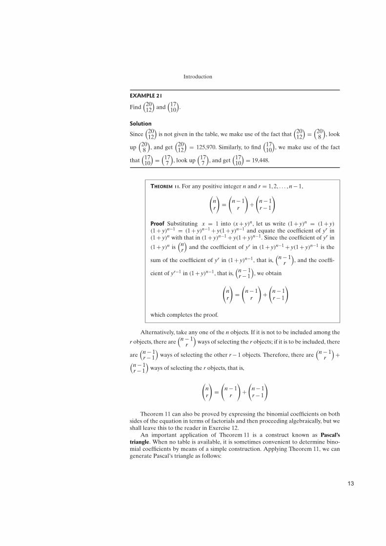
EXAMPLE 21
Find(
2012
)
and(
1710
)
.
Solution
Since(
2012
)
is not given in the table, we make use of the fact that(
2012
)
=(
208
)
, look
up(
208
)
, and get(
2012
)
= 125,970. Similarly, to find(
1710
)
, we make use of the fact
that(
1710
)
=(
177
)
, look up(
177
)
, and get(
1710
)
= 19,448.
THEOREM 11. For any positive integer n and r = 1, 2, . . . , n− 1,
(
n
r
)
=
(
n− 1r
)
+
(
n− 1r− 1
)
Proof Substituting x = 1 into (x+ y)n, let us write (1+ y)n = (1+ y)
(1+ y)n−1 = (1+ y)n−1+ y(1+ y)n−1 and equate the coefficient of yr in(1+ y)n with that in (1+ y)n−1+ y(1+ y)n−1. Since the coefficient of yr in
(1+ y)n is(
nr
)
and the coefficient of yr in (1+ y)n−1+ y(1+ y)n−1 is the
sum of the coefficient of yr in (1+ y)n−1, that is,(
n− 1r
)
, and the coeffi-
cient of yr−1 in (1+ y)n−1, that is,(
n− 1r− 1
)
, we obtain
(
n
r
)
=
(
n− 1r
)
+
(
n− 1r− 1
)
which completes the proof.
Alternatively, take any one of the n objects. If it is not to be included among the
r objects, there are(
n− 1r
)
ways of selecting the r objects; if it is to be included, there
are(
n− 1r− 1
)
ways of selecting the other r− 1 objects. Therefore, there are(
n− 1r
)
+(
n− 1r− 1
)
ways of selecting the r objects, that is,
(
n
r
)
=
(
n− 1r
)
+
(
n− 1r− 1
)
Theorem 11 can also be proved by expressing the binomial coefficients on bothsides of the equation in terms of factorials and then proceeding algebraically, but weshall leave this to the reader in Exercise 12.
An important application of Theorem 11 is a construct known as Pascal’s
triangle. When no table is available, it is sometimes convenient to determine bino-mial coefficients by means of a simple construction. Applying Theorem 11, we cangenerate Pascal’s triangle as follows:
"

Introduction
11 1
1 2 11 3 3 1
1 4 6 4 11 5 10 10 5 1. . . . . . . . . . . . . . . . . . . . . . . . . . . .
In this triangle, the first and last entries of each row are the numeral “1” each otherentry in any given row is obtained by adding the two entries in the preceding rowimmediately to its left and to its right.
To state the third theorem about binomial coefficients, let us make the following
definition:(
nr
)
= 0 whenever n is a positive integer and r is a positive integer greater
than n. (Clearly, there is no way in which we can select a subset that contains moreelements than the whole set itself.)
THEOREM 12.k∑
r=0
(
m
r
)(
n
k− r
)
=
(
m+n
k
)
Proof Using the same technique as in the proof of Theorem 11, let usprove this theorem by equating the coefficients of yk in the expressionson both sides of the equation
(1+ y)m+n = (1+ y)m(1+ y)n
The coefficient of yk in (1+y)m+n is(
m+n
k
)
, and the coefficient of yk in
(1+ y)m(1+ y)n =
(
m
0
)
+
(
m
1
)
y+ · · ·+
(
m
m
)
ym
*
(
n
0
)
+
(
n
1
)
y+ · · ·+
(
n
n
)
yn
is the sum of the products that we obtain by multiplying the constantterm of the first factor by the coefficient of yk in the second factor, thecoefficient of y in the first factor by the coefficient of yk−1 in the secondfactor, . . . , and the coefficient of yk in the first factor by the constant termof the second factor. Thus, the coefficient of yk in (1+ y)m(1+ y)n is
(
m
0
)(
n
k
)
+
(
m
1
)(
n
k− 1
)
+
(
m
2
)(
n
k− 2
)
+ · · ·+
(
m
k
)(
n
0
)
=k∑
r=0
(
m
r
)(
n
k− r
)
and this completes the proof.
#

Introduction
EXAMPLE 22
Verify Theorem 12 numerically for m = 2, n = 3, and k = 4.
Solution
Substituting these values, we get
(
20
)(
34
)
+
(
21
)(
33
)
+
(
22
)(
32
)
+
(
23
)(
31
)
+
(
24
)(
30
)
=
(
54
)
and since(
34
)
,(
23
)
, and(
24
)
equal 0 according to the definition on the previous page,
the equation reduces to
(
21
)(
33
)
+
(
22
)(
32
)
=
(
54
)
which checks, since 2 · 1+ 1 · 3 = 5.
Using Theorem 8, we can extend our discussion to multinomial coefficients, thatis, to the coefficients that arise in the expansion of (x1+ x2+ · · ·+ xk)n. The multi-nomial coefficient of the term x
r11 · x
r22 · . . . · xrk
k in the expansion of (x1+ x2+ · · ·+xk)n is
(
n
r1, r2, . . . , rk
)
=n!
r1! · r2! · . . . · rk!
EXAMPLE 23
What is the coefficient of x31x2x2
3 in the expansion of (x1+ x2+ x3)6?
Solution
Substituting n = 6, r1 = 3, r2 = 1, and r3 = 2 into the preceding formula, we get
6!
3! · 1! · 2!= 60
Exercises
1. An operation consists of two steps, of which the firstcan be made in n1 ways. If the first step is made in the ithway, the second step can be made in n2i ways.†
(a) Use a tree diagram to find a formula for the total num-ber of ways in which the total operation can be made.
(b) A student can study 0, 1, 2, or 3 hours for a historytest on any given day. Use the formula obtained in part(a) to verify that there are 13 ways in which the studentcan study at most 4 hours for the test on two consecutivedays.
2. With reference to Exercise 1, verify that if n2i equalsthe constant n2, the formula obtained in part (a) reducesto that of Theorem 1.
3. With reference to Exercise 1, suppose that there is athird step, and if the first step is made in the ith way andthe second step in the jth way, the third step can be madein n3ij ways.(a) Use a tree diagram to verify that the whole operationcan be made in
†The first subscript denotes the row to which a particular element belongs, and the second subscript denotes the column.
$

Introduction
n1∑
i=1
n2i∑
j=1
n3ij
different ways.
(b) With reference to part (b) of Exercise 1, use the for-mula of part (a) to verify that there are 32 ways in whichthe student can study at most 4 hours for the test on threeconsecutive days.
4. Show that if n2i equals the constant n2 and n3ij equalsthe constant n3, the formula of part (a) of Exercise 3reduces to that of Theorem 2.
5. In a two-team basketball play-off, the winner is the firstteam to win m games.(a) Counting separately the number of play-offs requiringm, m+ 1, . . . , and 2m− 1 games, show that the total num-ber of different outcomes (sequences of wins and lossesby one of the teams) is
2
[
(
m− 1m− 1
)
+(
mm− 1
)
+ · · ·+(
2m− 2m− 1
)
]
(b) How many different outcomes are there in a “2 outof 3” play-off, a “3 out of 5” play-off, and a “4 out of 7”play-off?
6. When n is large, n! can be approximated by means ofthe expression
√2πn
(
n
e
)n
called Stirling’s formula, where e is the base of naturallogarithms. (A derivation of this formula may be found inthe book by W. Feller cited among the references at theend of this chapter.)(a) Use Stirling’s formula to obtain approximations for10! and 12!, and find the percentage errors of theseapproximations by comparing them with the exact val-ues given in table Factorials and Binomial Coefficients of“Statistical Tables.”
(b) Use Stirling’s formula to obtain an approximation forthe number of 13-card bridge hands that can be dealt withan ordinary deck of 52 playing cards.
7. Using Stirling’s formula (see Exercise 6) to approxi-mate 2n! and n!, show that
(
2nn
)
√πn
22nL 1
8. In some problems of occupancy theory we are con-cerned with the number of ways in which certain distin-guishable objects can be distributed among individuals,urns, boxes, or cells. Find an expression for the number ofways in which r distinguishable objects can be distributedamong n cells, and use it to find the number of ways in
which three different books can be distributed among the12 students in an English literature class.
9. In some problems of occupancy theory we are con-cerned with the number of ways in which certain indistin-guishable objects can be distributed among individuals,urns, boxes, or cells. Find an expression for the numberof ways in which r indistinguishable objects can be dis-tributed among n cells, and use it to find the number ofways in which a baker can sell five (indistinguishable)loaves of bread to three customers. (Hint: We might arguethat L|LLL|L represents the case where the three cus-tomers buy one loaf, three loaves, and one loaf, respec-tively, and that LLLL||L represents the case where thethree customers buy four loaves, none of the loaves, andone loaf. Thus, we must look for the number of waysin which we can arrange the five L’s and the two verti-cal bars.)
10. In some problems of occupancy theory we are con-cerned with the number of ways in which certain indistin-guishable objects can be distributed among individuals,urns, boxes, or cells with at least one in each cell. Findan expression for the number of ways in which r indistin-guishable objects can be distributed among n cells withat least one in each cell, and rework the numerical partof Exercise 9 with each of the three customers getting atleast one loaf of bread.
11. Construct the seventh and eighth rows of Pascal’s tri-angle and write the binomial expansions of (x+ y)6 and(x+ y)7.
12. Prove Theorem 11 by expressing all the binomialcoefficients in terms of factorials and then simplifyingalgebraically.
13. Expressing the binomial coefficients in terms of fac-torials and simplifying algebraically, show that
(a)
(
nr
)
=n− r+ 1
r·(
nr− 1
)
;
(b)
(
nr
)
=n
n− r·(
n− 1r
)
;
(c) n
(
n− 1r
)
= (r+ 1)
(
nr+ 1
)
.
14. Substituting appropriate values for x and y into theformula of Theorem 9, show that
(a)
n∑
r=0
(
nr
)
= 2n;
(b)
n∑
r=0
(−1)r
(
nr
)
= 0;
(c)
n∑
r=0
(
nr
)
(a− 1)r = an.
%
Introduction
15. Repeatedly applying Theorem 11, show that
(
nr
)
=r+1∑
i=1
(
n− ir− i+ 1
)
16. Use Theorem 12 to show that
n∑
r=0
(
nr
)2
=(
2nn
)
17. Show thatn∑
r=0
r
(
nr
)
= n2n−1 by setting x = 1 in The-
orem 9, then differentiating the expressions on both sideswith respect to y, and finally substituting y = 1.
18. Rework Exercise 17 by making use of part (a) ofExercise 14 and part (c) of Exercise 13.
19. If n is not a positive integer or zero, the binomialexpansion of (1+ y)n yields, for −1 < y < 1, the infi-nite series
1+(
n1
)
y+(
n2
)
y2+(
n3
)
y3+ · · ·+(
nr
)
yr+ · · ·
where
(
nr
)
=n(n− 1) · . . . · (n− r+ 1)
r!for r = 1, 2, 3, . . . .
Use this generalized definition of binomial coefficientsto evaluate
(a)
(
124
)
and
(
−33
)
;
(b)√
5 writing√
5 = 2(1+ 14 )1/2 and using the first four
terms of the binomial expansion of (1+ 14 )1/2.
20. With reference to the generalized definition of bino-mial coefficients in Exercise 19, show that
(a)
(
−1r
)
= (−1)r;
(b)
(
−nr
)
= (−1)r
(
n+ r− 1r
)
for n > 0.
21. Find the coefficient of x2y3z3 in the expansion of(x+ y+ z)8.
22. Find the coefficient of x3y2z3w in the expansion of(2x+ 3y− 4z+w)9.
23. Show that
(
nn1, n2, . . . , nk
)
=(
n− 1n1− 1, n2, . . . , nk
)
+(
n− 1n1, n2− 1, . . . , nk
)
+ · · ·
+(
n− 1n1, n2, . . . , nk− 1
)
by expressing all these multinomial coefficients in termsof factorials and simplifying algebraically.
4 The Theory in Practice
Applications of the preceding theory of combinatorial methods and binomial coeffi-cients are quite straightforward, and a variety of them have been given in Sections 2and 3. The following examples illustrate further applications of this theory.
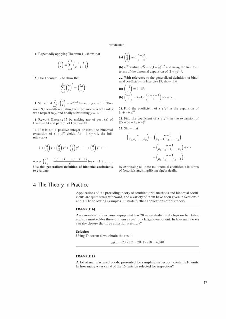
EXAMPLE 24
An assembler of electronic equipment has 20 integrated-circuit chips on her table,and she must solder three of them as part of a larger component. In how many wayscan she choose the three chips for assembly?
Solution
Using Theorem 6, we obtain the result
20P3 = 20!/17! = 20 · 19 · 18 = 6,840
EXAMPLE 25
A lot of manufactured goods, presented for sampling inspection, contains 16 units.In how many ways can 4 of the 16 units be selected for inspection?
&

Introduction
Solution
According to Theorem 7,
(
164
)
= 16!/4!12! = 16 · 15 · 14 · 13/4 · 3 · 2 · 1 = 1,092 ways
Applied Exercises SECS. 1–4
24. A thermostat will call for heat 0, 1, or 2 times a night.Construct a tree diagram to show that there are 10 differ-ent ways that it can turn on the furnace for a total of 6times over 4 nights.
25. On August 31 there are five wild-card terms in theAmerican League that can make it to the play-offs, andonly two will win spots. Draw a tree diagram which showsthe various possible play-off wild-card teams.
26. There are four routes, A, B, C, and D, between a per-son’s home and the place where he works, but route Bis one-way, so he cannot take it on the way to work, androute C is one-way, so he cannot take it on the way home.(a) Draw a tree diagram showing the various ways theperson can go to and from work.
(b) Draw a tree diagram showing the various ways hecan go to and from work without taking the same routeboth ways.
27. A person with $2 in her pocket bets $1, even money,on the flip of a coin, and she continues to bet $1 as longas she has any money. Draw a tree diagram to show thevarious things that can happen during the first four flipsof the coin. After the fourth flip of the coin, in how manyof the cases will she be(a) exactly even;
(b) exactly $2 ahead?
28. The pro at a golf course stocks two identical sets ofwomen’s clubs, reordering at the end of each day (fordelivery early the next morning) if and only if he has soldthem both. Construct a tree diagram to show that if hestarts on a Monday with two sets of the clubs, there arealtogether eight different ways in which he can make saleson the first two days of that week.
29. Suppose that in a baseball World Series (in which thewinner is the first team to win four games) the NationalLeague champion leads the American League championthree games to two. Construct a tree diagram to show thenumber of ways in which these teams may win or lose theremaining game or games.
30. If the NCAA has applications from six universitiesfor hosting its intercollegiate tennis championships in two
consecutive years, in how many ways can they select thehosts for these championships(a) if they are not both to be held at the same university;
(b) if they may both be held at the same university?
31. Counting the number of outcomes in games of chancehas been a popular pastime for many centuries. This wasof interest not only because of the gambling that wasinvolved, but also because the outcomes of games ofchance were often interpreted as divine intent. Thus, itwas just about a thousand years ago that a bishop in whatis now Belgium determined that there are 56 differentways in which three dice can fall provided one is inter-ested only in the overall result and not in which die doeswhat. He assigned a virtue to each of these possibilitiesand each sinner had to concentrate for some time on thevirtue that corresponded to his cast of the dice.(a) Find the number of ways in which three dice can allcome up with the same number of points.
(b) Find the number of ways in which two of the threedice can come up with the same number of points, whilethe third comes up with a different number of points.
(c) Find the number of ways in which all three of the dicecan come up with a different number of points.
(d) Use the results of parts (a), (b), and (c) to verifythe bishop’s calculations that there are altogether 56possibilities.
32. In a primary election, there are four candidates formayor, five candidates for city treasurer, and two candi-dates for county attorney.(a) In how many ways can a voter mark his ballot for allthree of these offices?
(b) In how many ways can a person vote if he exerciseshis option of not voting for a candidate for any or all ofthese offices?
33. The five finalists in the Miss Universe contest are MissArgentina, Miss Belgium, Miss U.S.A., Miss Japan, andMiss Norway. In how many ways can the judges choose(a) the winner and the first runner-up;
(b) the winner, the first runner-up, and the secondrunner-up?
'
Introduction
34. A multiple-choice test consists of 15 questions, eachpermitting a choice of three alternatives. In how many dif-ferent ways can a student check off her answers to thesequestions?
35. Determine the number of ways in which a distributorcan choose 2 of 15 warehouses to ship a large order.
36. The price of a European tour includes four stopoversto be selected from among 10 cities. In how many differ-ent ways can one plan such a tour(a) if the order of the stopovers matters;
(b) if the order of the stopovers does not matter?
37. A carton of 15 light bulbs contains one that is defec-tive. In how many ways can an inspector choose 3 of thebulbs and(a) get the one that is defective;
(b) not get the one that is defective?
38. In how many ways can a television director sched-ule a sponsor’s six different commercials during the sixtime slots allocated to commercials during a two-hourprogram?
39. In how many ways can the television director of Exer-cise 38 fill the six time slots for commercials if there arethree different sponsors and the commercial for each is tobe shown twice?
40. In how many ways can five persons line up to get ona bus? In how many ways can they line up if two of thepersons refuse to follow each other?
41. In how many ways can eight persons form a circle fora folk dance?
42. How many permutations are there of the letters in theword(a) “great”;
(b) “greet”?
43. How many distinct permutations are there of the let-ters in the word “statistics”? How many of these beginand end with the letter s?
44. A college team plays 10 football games during a sea-son. In how many ways can it end the season with fivewins, four losses, and one tie?
45. If eight persons are having dinner together, in howmany different ways can three order chicken, four ordersteak, and one order lobster?
46. In Example 4 we showed that a true–false test consist-ing of 20 questions can be marked in 1,048,576 differentways. In how many ways can each question be markedtrue or false so that
(a) 7 are right and 13 are wrong;
(b) 10 are right and 10 are wrong;
(c) at least 17 are right?
47. Among the seven nominees for two vacancies on acity council are three men and four women. In how manyways can these vacancies be filled(a) with any two of the seven nominees;
(b) with any two of the four women;
(c) with one of the men and one of the women?
48. A shipment of 10 television sets includes three thatare defective. In how many ways can a hotel purchasefour of these sets and receive at least two of the defectivesets?
49. Ms. Jones has four skirts, seven blouses, and threesweaters. In how many ways can she choose two of theskirts, three of the blouses, and one of the sweaters to takealong on a trip?
50. How many different bridge hands are possible con-taining five spades, three diamonds, three clubs, and twohearts?
51. Find the number of ways in which one A, three B’s,two C’s, and one F can be distributed among seven stu-dents taking a course in statistics.
52. An art collector, who owns 10 paintings by famousartists, is preparing her will. In how many different wayscan she leave these paintings to her three heirs?
53. A baseball fan has a pair of tickets for six differenthome games of the Chicago Cubs. If he has five friendswho like baseball, in how many different ways can he takeone of them along to each of the six games?
54. At the end of the day, a bakery gives everything thatis unsold to food banks for the needy. If it has 12 applepies left at the end of a given day, in how many differentways can it distribute these pies among six food banks forthe needy?
55. With reference to Exercise 54, in how many differ-ent ways can the bakery distribute the 12 apple piesif each of the six food banks is to receive at leastone pie?
56. On a Friday morning, the pro shop of a tennis clubhas 14 identical cans of tennis balls. If they are all soldby Sunday night and we are interested only in how manywere sold on each day, in how many different ways couldthe tennis balls have been sold on Friday, Saturday, andSunday?
57. Rework Exercise 56 given that at least two of the cansof tennis balls were sold on each of the three days.
(

Introduction
References
Among the books on the history of statistics there are
Walker, H. M., Studies in the History of StatisticalMethod. Baltimore: The Williams & Wilkins Company,1929,
Westergaard, H., Contributions to the History of Statis-tics. London: P. S. King & Son, 1932,
and the more recent publications
Kendall, M. G., and Plackett, R. L., eds., Studies in theHistory of Statistics and Probability, Vol. II. New York:Macmillan Publishing Co., Inc., 1977,
Pearson, E. S., and Kendall, M. G., eds., Studies in theHistory of Statistics and Probability. Darien, Conn.:Hafner Publishing Co., Inc., 1970,
Porter, T. M., The Rise of Statistical Thinking, 1820–1900. Princeton, N.J.: Princeton University Press, 1986,
andStigler, S. M., The History of Statistics. Cambridge,
Mass.: Harvard University Press, 1986.
A wealth of material on combinatorial methods can befound in
Cohen, D. A., Basic Techniques of Combinatorial The-ory. New York: John Wiley & Sons, Inc., 1978,
Eisen, M., Elementary Combinatorial Analysis. NewYork: Gordon and Breach, Science Publishers, Inc.,1970,
Feller, W., An Introduction to Probability Theory and ItsApplications, Vol. I, 3rd ed. New York: John Wiley &Sons, Inc., 1968,
Niven, J., Mathematics of Choice. New York: RandomHouse, Inc., 1965,
Roberts, F. S., Applied Combinatorics. Upper SaddleRiver, N.J.: Prentice Hall, 1984,
andWhitworth, W. A., Choice and Chance, 5th ed. New
York: Hafner Publishing Co., Inc., 1959, which hasbecome a classic in this field.
More advanced treatments may be found in
Beckenbach, E. F., ed., Applied Combinatorial Mathe-matics. New York: John Wiley & Sons, Inc., 1964,
David, F. N., and BARTON, D. E., CombinatorialChance. New York: Hafner Publishing Co., Inc., 1962,
andRiordan, J., An Introduction to Combinatorial Analysis.
New York: John Wiley & Sons, Inc., 1958.
Answers to Odd-Numbered Exercises
1 (a)
n∑
i=1
n2ni.
5 (b) 6, 20, and 70.
9
(
r+n− 1r
)
and 21.
11 Seventh row: 1, 6, 15, 20, 15, 6, 1; Eighth row: 1, 7, 21, 35,35, 27, 7, 1.
19 (a) −15384 and −10; (b) 2.230.
21 560.
27 (a) 5; (b) 4.
31 (a) 6; (b) 30; (c) 20; (d) 56.
33 (a) 20; (b) 60.
35 (a) 105.
37 (a) 91; (b) 364.
39 90.
41 5040.
43 50,400 and 3360.
45 280.
47 (a) 21; (b) 6; (c) 12.
49 630.
51 420.
53 15,625.
55 462.
57 45.
!)

Probability
1 Introduction2 Sample Spaces3 Events4 The Probability of an Event5 Some Rules of Probability
6 Conditional Probability7 Independent Events8 Bayes’ Theorem9 The Theory in Practice
1 Introduction Historically, the oldest way of defining probabilities, the classical probability con-
cept, applies when all possible outcomes are equally likely, as is presumably the casein most games of chance. We can then say that if there are N equally likely possibili-
ties, of which one must occur and n are regarded as favorable, or as a “success,” then
the probability of a “success” is given by the ratio nN .
EXAMPLE 1
What is the probability of drawing an ace from an ordinary deck of 52 playing cards?
Solution
Since there are n = 4 aces among the N = 52 cards, the probability of drawingan ace is 4
52 = 113 . (It is assumed, of course, that each card has the same chance of
being drawn.)
Although equally likely possibilities are found mostly in games of chance, theclassical probability concept applies also in a great variety of situations where gam-bling devices are used to make random selections—when office space is assigned toteaching assistants by lot, when some of the families in a township are chosen in sucha way that each one has the same chance of being included in a sample study, whenmachine parts are chosen for inspection so that each part produced has the samechance of being selected, and so forth.
A major shortcoming of the classical probability concept is its limited applica-bility, for there are many situations in which the possibilities that arise cannot allbe regarded as equally likely. This would be the case, for instance, if we are con-cerned with the question whether it will rain on a given day, if we are concernedwith the outcome of an election, or if we are concerned with a person’s recoveryfrom a disease.
Among the various probability concepts, most widely held is the frequency inter-
pretation, according to which the probability of an event (outcome or happening) isthe proportion of the time that events of the same kind will occur in the long run.If we say that the probability is 0.84 that a jet from Los Angeles to San Franciscowill arrive on time, we mean (in accordance with the frequency interpretation) thatsuch flights arrive on time 84 percent of the time. Similarly, if the weather bureau
From Chapter 2 of John E. Freund’s Mathematical Statistics with Applications,Eighth Edition. Irwin Miller, Marylees Miller. Copyright 2014 by Pearson Education, Inc.All rights reserved.
!

Probability
predicts that there is a 30 percent chance for rain (that is, a probability of 0.30), thismeans that under the same weather conditions it will rain 30 percent of the time.More generally, we say that an event has a probability of, say, 0.90, in the same sensein which we might say that our car will start in cold weather 90 percent of the time.We cannot guarantee what will happen on any particular occasion—the car may startand then it may not—but if we kept records over a long period of time, we shouldfind that the proportion of “successes” is very close to 0.90.
The approach to probability that we shall use in this chapter is the axiomatic
approach, in which probabilities are defined as “mathematical objects” that behaveaccording to certain well-defined rules. Then, any one of the preceding probabilityconcepts, or interpretations, can be used in applications as long as it is consistentwith these rules.
2 Sample Spaces
Since all probabilities pertain to the occurrence or nonoccurrence of events, let usexplain first what we mean here by event and by the related terms experiment, out-
come, and sample space.It is customary in statistics to refer to any process of observation or measure-
ment as an experiment. In this sense, an experiment may consist of the simple pro-cess of checking whether a switch is turned on or off; it may consist of counting theimperfections in a piece of cloth; or it may consist of the very complicated processof determining the mass of an electron. The results one obtains from an experi-ment, whether they are instrument readings, counts, “yes” or “no” answers, or valuesobtained through extensive calculations, are called the outcomes of the experiment.
DEFINITION 1. SAMPLE SPACE. The set of all possible outcomes of an experiment is
called the sample space and it is usually denoted by the letter S. Each outcome
in a sample space is called an element of the sample space, or simply a samplepoint.
If a sample space has a finite number of elements, we may list the elements inthe usual set notation; for instance, the sample space for the possible outcomes ofone flip of a coin may be written
S = {H, T}
where H and T stand for head and tail. Sample spaces with a large or infinite numberof elements are best described by a statement or rule; for example, if the possibleoutcomes of an experiment are the set of automobiles equipped with satellite radios,the sample space may be written
S = {x|x is an automobile with a satellite radio}
This is read “S is the set of all x such that x is an automobile with a satellite radio.”Similarly, if S is the set of odd positive integers, we write
S = {2k + 1|k = 0, 1, 2, . . .}
How we formulate the sample space for a given situation will depend on theproblem at hand. If an experiment consists of one roll of a die and we are interestedin which face is turned up, we would use the sample space
!!

Probability
S1 = {1, 2, 3, 4, 5, 6}
However, if we are interested only in whether the face turned up is even or odd, wewould use the sample space
S2 = {even, odd}
This demonstrates that different sample spaces may well be used to describe anexperiment. In general, it is desirable to use sample spaces whose elements cannot
be divided (partitioned or separated) into more primitive or more elementary kinds
of outcomes. In other words, it is preferable that an element of a sample space not
represent two or more outcomes that are distinguishable in some way. Thus, in thepreceding illustration S1 would be preferable to S2.
EXAMPLE 2
Describe a sample space that might be appropriate for an experiment in which weroll a pair of dice, one red and one green. (The different colors are used to emphasizethat the dice are distinct from one another.)
Solution
The sample space that provides the most information consists of the 36 points given by
S1 = {(x, y)|x = 1, 2, . . . , 6; y = 1, 2, . . . , 6}
where x represents the number turned up by the red die and y represents the numberturned up by the green die. A second sample space, adequate for most purposes(though less desirable in general as it provides less information), is given by
S2 = {2, 3, 4, . . . , 12}
where the elements are the totals of the numbers turned up by the two dice.
Sample spaces are usually classified according to the number of elements thatthey contain. In the preceding example the sample spaces S1 and S2 contained afinite number of elements; but if a coin is flipped until a head appears for the firsttime, this could happen on the first flip, the second flip, the third flip, the fourth flip,. . ., and there are infinitely many possibilities. For this experiment we obtain thesample space
S = {H, TH, TTH, TTTH, TTTTH, . . .}
with an unending sequence of elements. But even here the number of elements canbe matched one-to-one with the whole numbers, and in this sense the sample spaceis said to be countable. If a sample space contains a finite number of elements or aninfinite though countable number of elements, it is said to be discrete.
The outcomes of some experiments are neither finite nor countably infinite. Suchis the case, for example, when one conducts an investigation to determine the dis-tance that a certain make of car will travel over a prescribed test course on 5 litersof gasoline. If we assume that distance is a variable that can be measured to anydesired degree of accuracy, there is an infinity of possibilities (distances) that can-not be matched one-to-one with the whole numbers. Also, if we want to measurethe amount of time it takes for two chemicals to react, the amounts making up thesample space are infinite in number and not countable. Thus, sample spaces need
!"

Probability
not be discrete. If a sample space consists of a continuum, such as all the points ofa line segment or all the points in a plane, it is said to be continuous. Continuoussample spaces arise in practice whenever the outcomes of experiments are measure-ments of physical properties, such as temperature, speed, pressure, length, . . ., thatare measured on continuous scales.
3 Events In many problems we are interested in results that are not given directly by a specificelement of a sample space.
EXAMPLE 3
With reference to the first sample space S1 on the previous page, describe the eventA that the number of points rolled with the die is divisible by 3.
Solution
Among 1, 2, 3, 4, 5, and 6, only 3 and 6 are divisible by 3. Therefore, A is representedby the subset {3, 6} of the sample space S1.
EXAMPLE 4
With reference to the sample space S1 of Example 2, describe the event B that thetotal number of points rolled with the pair of dice is 7.
Solution
Among the 36 possibilities, only (1, 6), (2, 5), (3, 4), (4, 3), (5, 2), and (6, 1) yielda total of 7. So, we write
B = {(1, 6), (2, 5), (3, 4), (4, 3), (5, 2), (6, 1)}
Note that in Figure 1 the event of rolling a total of 7 with the two dice is representedby the set of points inside the region bounded by the dotted line.
1
2
3
4
5
6
1 2 3 4 5Red die
Greendie
6
Figure 1. Rolling a total of 7 with a pair of dice.
!#

Probability
In the same way, any event (outcome or result) can be identified with a collectionof points, which constitute a subset of an appropriate sample space. Such a subsetconsists of all the elements of the sample space for which the event occurs, and inprobability and statistics we identify the subset with the event.
DEFINITION 2. EVENT. An event is a subset of a sample space.
EXAMPLE 5
If someone takes three shots at a target and we care only whether each shot is a hitor a miss, describe a suitable sample space, the elements of the sample space thatconstitute event M that the person will miss the target three times in a row, and theelements of event N that the person will hit the target once and miss it twice.
Solution
If we let 0 and 1 represent a miss and a hit, respectively, the eight possibilities (0, 0, 0),(1, 0, 0), (0, 1, 0), (0, 0, 1), (1, 1, 0), (1, 0, 1), (0, 1, 1), and (1, 1, 1) may be displayedas in Figure 2. Thus, it can be seen that
M = {(0, 0, 0)}
and
N = {(1, 0, 0), (0, 1, 0), (0, 0, 1)}
(0, 1, 1)
(0, 1, 0)
(0, 0, 0)
(0, 0, 1)(1, 0, 1)
(1, 1, 1)
(1, 0, 0)
(1, 1, 0)
Thirdshot
Firstshot
Secondshot
Figure 2. Sample space for Example 5.
EXAMPLE 6
Construct a sample space for the length of the useful life of a certain electroniccomponent and indicate the subset that represents the event F that the componentfails before the end of the sixth year.
!$

Probability
Solution
If t is the length of the component’s useful life in years, the sample space may bewritten S = {t|t G 0}, and the subset F = {t|0 F t < 6} is the event that the componentfails before the end of the sixth year.
According to our definition, any event is a subset of an appropriate samplespace, but it should be observed that the converse is not necessarily true. For dis-crete sample spaces, all subsets are events, but in the continuous case some ratherabstruse point sets must be excluded for mathematical reasons. This is discussed fur-ther in some of the more advanced texts listed among the references at the end ofthis chapter.
In many problems of probability we are interested in events that are actuallycombinations of two or more events, formed by taking unions, intersections, andcomplements. Although the reader must surely be familiar with these terms, let usreview briefly that, if A and B are any two subsets of a sample space S, their unionA ∪ B is the subset of S that contains all the elements that are either in A, in B,or in both; their intersection A ∩ B is the subset of S that contains all the elementsthat are in both A and B; and the complement A′ of A is the subset of S that con-tains all the elements of S that are not in A. Some of the rules that control theformation of unions, intersections, and complements may be found in Exercises 1through 4.
Sample spaces and events, particularly relationships among events, are oftendepicted by means of Venn diagrams, in which the sample space is represented bya rectangle, while events are represented by regions within the rectangle, usually bycircles or parts of circles. For instance, the shaded regions of the four Venn diagramsof Figure 3 represent, respectively, event A, the complement of event A, the unionof events A and B, and the intersection of events A and B. When we are dealingwith three events, we usually draw the circles as in Figure 4. Here, the regions arenumbered 1 through 8 for easy reference.
Figure 3. Venn diagrams.
!%

Probability
Figure 4. Venn diagram.
Figure 5. Diagrams showing special relationships among events.
To indicate special relationships among events, we sometimes draw diagramslike those of Figure 5. Here, the one on the left serves to indicate that events A andB are mutually exclusive.
DEFINITION 3. MUTUALLY EXCLUSIVE EVENTS. Two events having no elements in com-
mon are said to be mutually exclusive.
When A and B are mutually exclusive, we write A ∩ B = ∅, where ∅ denotesthe empty set, which has no elements at all. The diagram on the right serves toindicate that A is contained in B, and symbolically we express this by writingA ( B.
Exercises
1. Use Venn diagrams to verify that(a) (A ∪ B)∪ C is the same event as A ∪ (B ∪ C);
(b) A ∩ (B ∪ C) is the same event as (A ∩ B)∪ (A ∩ C);
(c) A ∪ (B ∩ C) is the same event as (A ∪ B)∩ (A ∪ C).
2. Use Venn diagrams to verify the two De Morgan laws:(a) (A ∩ B)′ = A′ ∪ B′; (b) (A ∪ B)′ = A′ ∩ B′.
3. Use Venn diagrams to verify that(a) (A ∩ B)∪ (A ∩ B′) = A;
(b) (A ∩ B)∪ (A ∩ B′)∪ (A′ ∩ B) = A ∪ B;
(c) A ∪ (A′ ∩ B) = A ∪ B.
4. Use Venn diagrams to verify that if A is contained inB, then A ∩ B = A and A ∩ B′ = ∅.
!

Probability
4 The Probability of an Event
To formulate the postulates of probability, we shall follow the practice of denotingevents by means of capital letters, and we shall write the probability of event A asP(A), the probability of event B as P(B), and so forth. The following postulates ofprobability apply only to discrete sample spaces, S.
POSTULATE 1 The probability of an event is a nonnegative real number;that is, P(A) G 0 for any subset A of S.
POSTULATE 2 P(S) = 1.POSTULATE 3 If A1, A2, A3, . . ., is a finite or infinite sequence of mutually
exclusive events of S, then
P(A1 ∪ A2 ∪ A3 ∪ · · · ) = P(A1)+ P(A2)+ P(A3)+ · · ·
Postulates per se require no proof, but if the resulting theory is to be applied,we must show that the postulates are satisfied when we give probabilities a “real”meaning. Let us illustrate this in connection with the frequency interpretation; therelationship between the postulates and the classical probability concept will bediscussed below, while the relationship between the postulates and subjective prob-abilities is left for the reader to examine in Exercises 16 and 82.
Since proportions are always positive or zero, the first postulate is in completeagreement with the frequency interpretation. The second postulate states indirectlythat certainty is identified with a probability of 1; after all, it is always assumed thatone of the possibilities in S must occur, and it is to this certain event that we assigna probability of 1. As far as the frequency interpretation is concerned, a probabilityof 1 implies that the event in question will occur 100 percent of the time or, in otherwords, that it is certain to occur.
Taking the third postulate in the simplest case, that is, for two mutually exclusiveevents A1 and A2, it can easily be seen that it is satisfied by the frequency interpreta-tion. If one event occurs, say, 28 percent of the time, another event occurs 39 percentof the time, and the two events cannot both occur at the same time (that is, they aremutually exclusive), then one or the other will occur 28 + 39 = 67 percent of thetime. Thus, the third postulate is satisfied, and the same kind of argument applieswhen there are more than two mutually exclusive events.
Before we study some of the immediate consequences of the postulates of prob-ability, let us emphasize the point that the three postulates do not tell us how toassign probabilities to events; they merely restrict the ways in which it can be done.
EXAMPLE 7
An experiment has four possible outcomes, A, B, C, and D, that are mutually exclu-sive. Explain why the following assignments of probabilities are not permissible:
(a) P(A) = 0.12, P(B) = 0.63, P(C) = 0.45, P(D) = −0.20;
(b) P(A) = 9120 , P(B) = 45
120 , P(C) = 27120 , P(D) = 46
120 .
Solution
(a) P(D) = −0.20 violates Postulate 1;
(b) P(S) = P(A ∪ B ∪ C ∪ D) = 9120 + 45
120 + 27120 + 46
120 = 127120 Z 1, and this violates
Postulate 2.
"

Probability
Of course, in actual practice probabilities are assigned on the basis of past expe-rience, on the basis of a careful analysis of all underlying conditions, on the basisof subjective judgments, or on the basis of assumptions—sometimes the assumptionthat all possible outcomes are equiprobable.
To assign a probability measure to a sample space, it is not necessary to specifythe probability of each possible subset. This is fortunate, for a sample space with asfew as 20 possible outcomes has already 220 = 1,048,576 subsets, and the numberof subsets grows very rapidly when there are 50 possible outcomes, 100 possibleoutcomes, or more. Instead of listing the probabilities of all possible subsets, weoften list the probabilities of the individual outcomes, or sample points of S, andthen make use of the following theorem.
THEOREM 1. If A is an event in a discrete sample space S, then P(A) equalsthe sum of the probabilities of the individual outcomes comprising A.
Proof Let O1, O2, O3, . . ., be the finite or infinite sequence of outcomesthat comprise the event A. Thus,
A = O1 ∪ O2 ∪ O3 · · ·
and since the individual outcomes, the O’s, are mutually exclusive, thethird postulate of probability yields
P(A) = P(O1)+ P(O2)+ P(O3)+ · · ·
This completes the proof.
To use this theorem, we must be able to assign probabilities to the individualoutcomes of experiments. How this is done in some special situations is illustratedby the following examples.
EXAMPLE 8
If we twice flip a balanced coin, what is the probability of getting at least one head?
Solution
The sample space is S = {HH, HT, TH, TT}, where H and T denote head and tail.Since we assume that the coin is balanced, these outcomes are equally likely and weassign to each sample point the probability 1
4 . Letting A denote the event that wewill get at least one head, we get A = {HH, HT, TH} and
P(A) = P(HH)+ P(HT)+ P(TH)
=1
4+
1
4+
1
4
=3
4
#

Probability
EXAMPLE 9
A die is loaded in such a way that each odd number is twice as likely to occur as eacheven number. Find P(G), where G is the event that a number greater than 3 occurson a single roll of the die.
Solution
The sample space is S = {1, 2, 3, 4, 5, 6}. Hence, if we assign probability w to eacheven number and probability 2w to each odd number, we find that 2w + w + 2w +w + 2w + w = 9w = 1 in accordance with Postulate 2. It follows that w = 1
9 and
P(G) =1
9+
2
9+
1
9=
4
9
If a sample space is countably infinite, probabilities will have to be assigned tothe individual outcomes by means of a mathematical rule, preferably by means of aformula or equation.
EXAMPLE 10
If, for a given experiment, O1, O2, O3, . . ., is an infinite sequence of outcomes, ver-ify that
P(Oi) =(
1
2
)i
for i = 1, 2, 3, . . .
is, indeed, a probability measure.
Solution
Since the probabilities are all positive, it remains to be shown that P(S) = 1. Getting
P(S) =1
2+
1
4+
1
8+
1
16+ · · ·
and making use of the formula for the sum of the terms of an infinite geometricprogression, we find that
P(S) =12
1 − 12
= 1
In connection with the preceding example, the word “sum” in Theorem 1 willhave to be interpreted so that it includes the value of an infinite series.
The probability measure of Example 10 would be appropriate, for example, ifOi is the event that a person flipping a balanced coin will get a tail for the first timeon the ith flip of the coin. Thus, the probability that the first tail will come on thethird, fourth, or fifth flip of the coin is
(1
2
)3
+(
1
2
)4
+(
1
2
)5
=7
32
and the probability that the first tail will come on an odd-numbered flip of the coin is
(1
2
)1
+(
1
2
)3
+(
1
2
)5
+ · · · =12
1 − 14
=2
3
$%
Probability
Here again we made use of the formula for the sum of the terms of an infinite geo-metric progression.
If an experiment is such that we can assume equal probabilities for all the samplepoints, as was the case in Example 8, we can take advantage of the following specialcase of Theorem 1.
THEOREM 2. If an experiment can result in any one of N different equallylikely outcomes, and if n of these outcomes together constitute event A,then the probability of event A is
P(A) =n
N
Proof Let O1, O2, . . . , ON represent the individual outcomes in S, each
with probability1
N. If A is the union of n of these mutually exclusive
outcomes, and it does not matter which ones, then
P(A) = P(O1 ∪ O2 ∪ · · · ∪ On)
= P(O1)+ P(O2)+ · · · + P(On)
=1
N+
1
N+ · · · +
1
N︸ ︷︷ ︸
n terms
=n
N
Observe that the formula P(A) =n
Nof Theorem 2 is identical with the one for
the classical probability concept (see below). Indeed, what we have shown here isthat the classical probability concept is consistent with the postulates ofprobability—it follows from the postulates in the special case where the individualoutcomes are all equiprobable.
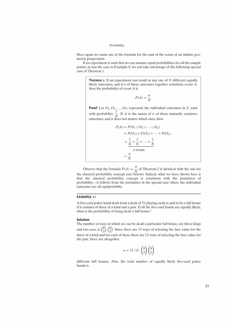
EXAMPLE 11
A five-card poker hand dealt from a deck of 52 playing cards is said to be a full houseif it consists of three of a kind and a pair. If all the five-card hands are equally likely,what is the probability of being dealt a full house?
Solution
The number of ways in which we can be dealt a particular full house, say three kings
and two aces, is(
43
) (42
)
. Since there are 13 ways of selecting the face value for the
three of a kind and for each of these there are 12 ways of selecting the face value forthe pair, there are altogether
n = 13 · 12 ·(
43
)(
42
)
different full houses. Also, the total number of equally likely five-card pokerhands is
$&

Probability
N =(
525
)
and it follows by Theorem 2 that the probability of getting a full house is
P(A) =n
N=
13 · 12
(
43
)(
42
)
(
525
) = 0.0014
5 Some Rules of Probability
Based on the three postulates of probability, we can derive many other rules thathave important applications. Among them, the next four theorems are immediateconsequences of the postulates.
THEOREM 3. If A and A′ are complementary events in a sample space S, then
P(A′) = 1 − P(A)
Proof In the second and third steps of the proof that follows, we makeuse of the definition of a complement, according to which A and A′ aremutually exclusive and A ∪ A′ = S. Thus, we write
1 = P(S) (by Postulate 2)
= P(A ∪ A′)
= P(A)+ P(A′) (by Postulate 3)
and it follows that P(A′) = 1 − P(A).
In connection with the frequency interpretation, this result implies that if anevent occurs, say, 37 percent of the time, then it does not occur 63 percent ofthe time.
THEOREM 4. P(∅) = 0 for any sample space S.
Proof Since S and ∅ are mutually exclusive and S ∪∅ = S in accordancewith the definition of the empty set ∅, it follows that
P(S) = P(S ∪∅)
= P(S)+ P(∅) (by Postulate 3)
and, hence, that P(∅) = 0.
It is important to note that it does not necessarily follow from P(A) = 0 thatA = ∅. In practice, we often assign 0 probability to events that, in colloquial terms,
$

Probability
would not happen in a million years. For instance, there is the classical example thatwe assign a probability of 0 to the event that a monkey set loose on a typewriter willtype Plato’s Republic word for word without a mistake. The fact that P(A) = 0 doesnot imply that A = ∅ is of relevance, especially, in the continuous case.
THEOREM 5. If A and B are events in a sample space S and A ( B, thenP(A) F P(B).
Proof Since A ( B, we can write
B = A ∪ (A′ ∩ B)
as can easily be verified by means of a Venn diagram. Then, since A andA′ ∩ B are mutually exclusive, we get
P(B) = P(A)+ P(A′ ∩ B) (by Postulate 3)
G P(A) (by Postulate 1)
In words, this theorem states that if A is a subset of B, then P(A) cannot begreater than P(B). For instance, the probability of drawing a heart from an ordinarydeck of 52 playing cards cannot be greater than the probability of drawing a red card.Indeed, the probability of drawing a heart is 1
4 , compared with 12 , the probability of
drawing a red card.
THEOREM 6. 0 F P(A) F 1 for any event A.
Proof Using Theorem 5 and the fact that ∅( A ( S for any event A in S,we have
P(∅) F P(A) F P(S)
Then, P(∅) = 0 and P(S) = 1 leads to the result that
0 F P(A) F 1
The third postulate of probability is sometimes referred to as the special addi-
tion rule; it is special in the sense that events A1, A2, A3, . . ., must all be mutuallyexclusive. For any two events A and B, there exists the general addition rule, or theinclusion–exclusion principle:
THEOREM 7. If A and B are any two events in a sample space S, then
P(A ∪ B) = P(A)+ P(B)− P(A ∩ B)
Proof Assigning the probabilities a, b, and c to the mutually exclusiveevents A ∩ B, A ∩ B′, and A′ ∩ B as in the Venn diagram of Figure 6, wefind that
P(A ∪ B) = a + b + c
= (a + b)+ (c + a)− a
= P(A)+ P(B)− P(A ∩ B)
$$

Probability
A B
b a c
Figure 6. Venn diagram for proof of Theorem 7.
EXAMPLE 12
In a large metropolitan area, the probabilities are 0.86, 0.35, and 0.29, respectively,that a family (randomly chosen for a sample survey) owns a color television set, aHDTV set, or both kinds of sets. What is the probability that a family owns either orboth kinds of sets?
Solution
If A is the event that a family in this metropolitan area owns a color television setand B is the event that it owns a HDTV set, we have P(A) = 0.86, P(B) = 0.35, andP(A ∩ B) = 0.29; substitution into the formula of Theorem 7 yields
P(A ∪ B) = 0.86 + 0.35 − 0.29
= 0.92
EXAMPLE 13
Near a certain exit of I-17, the probabilities are 0.23 and 0.24, respectively, thata truck stopped at a roadblock will have faulty brakes or badly worn tires. Also,the probability is 0.38 that a truck stopped at the roadblock will have faulty brakesand/or badly worn tires. What is the probability that a truck stopped at this roadblockwill have faulty brakes as well as badly worn tires?
Solution
If B is the event that a truck stopped at the roadblock will have faulty brakes and T
is the event that it will have badly worn tires, we have P(B) = 0.23, P(T) = 0.24, andP(B ∪ T) = 0.38; substitution into the formula of Theorem 7 yields
0.38 = 0.23 + 0.24 − P(B ∩ T)
Solving for P(B ∩ T), we thus get
P(B ∩ T) = 0.23 + 0.24 − 0.38 = 0.09
Repeatedly using the formula of Theorem 7, we can generalize this addition ruleso that it will apply to any number of events. For instance, for three events we obtainthe following theorem.
$'

Probability
THEOREM 8. If A, B, and C are any three events in a sample space S, then
P(A ∪ B ∪ C) = P(A)+ P(B)+ P(C)− P(A ∩ B)− P(A ∩ C)
− P(B ∩ C)+ P(A ∩ B ∩ C)
Proof Writing A ∪ B ∪ C as A ∪ (B ∪ C) and using the formula of Theo-rem 7 twice, once for P[A ∪ (B ∪ C)] and once for P(B ∪ C), we get
P(A ∪ B ∪ C) = P[A ∪ (B ∪ C)]
= P(A)+ P(B ∪ C)− P[A ∩ (B ∪ C)]
= P(A)+ P(B)+ P(C)− P(B ∩ C)
− P[A ∩ (B ∪ C)]
Then, using the distributive law that the reader was asked to verify in part(b) of Exercise 1, we find that
P[A ∩ (B ∪ C)] = P[(A ∩ B)∪ (A ∩ C)]
= P(A ∩ B)+ P(A ∩ C)− P[(A ∩ B)∩ (A ∩ C)]
= P(A ∩ B)+ P(A ∩ C)− P(A ∩ B ∩ C)
and hence that
P(A ∪ B ∪ C) = P(A)+ P(B)+ P(C)− P(A ∩ B)− P(A ∩ C)
− P(B ∩ C)+ P(A ∩ B ∩ C)
(In Exercise 12 the reader will be asked to give an alternative proof of this the-orem, based on the method used in the text to prove Theorem 7.)
EXAMPLE 14
If a person visits his dentist, suppose that the probability that he will have his teethcleaned is 0.44, the probability that he will have a cavity filled is 0.24, the probabilitythat he will have a tooth extracted is 0.21, the probability that he will have his teethcleaned and a cavity filled is 0.08, the probability that he will have his teeth cleanedand a tooth extracted is 0.11, the probability that he will have a cavity filled anda tooth extracted is 0.07, and the probability that he will have his teeth cleaned,a cavity filled, and a tooth extracted is 0.03. What is the probability that a personvisiting his dentist will have at least one of these things done to him?
Solution
If C is the event that the person will have his teeth cleaned, F is the event that hewill have a cavity filled, and E is the event that he will have a tooth extracted, weare given P(C) = 0.44, P(F) = 0.24, P(E) = 0.21, P(C ∩ F) = 0.08, P(C ∩ E) = 0.11,P(F ∩ E) = 0.07, and P(C ∩ F ∩ E) = 0.03, and substitution into the formula ofTheorem 8 yields
P(C ∪ F ∪ E) = 0.44 + 0.24 + 0.21 − 0.08 − 0.11 − 0.07 + 0.03
= 0.66
$(

Probability
Exercises
5. Use parts (a) and (b) of Exercise 3 to show that(a) P(A) G P(A ∩ B);
(b) P(A) F P(A ∪ B).
6. Referring to Figure 6, verify that
P(A ∩ B′) = P(A)− P(A ∩ B)
7. Referring to Figure 6 and letting P(A′ ∩ B′) = d, ver-ify that
P(A′ ∩ B′) = 1 − P(A)− P(B)+ P(A ∩ B)
8. The event that “A or B but not both” will occur can bewritten as
(A ∩ B′)∪ (A′ ∩ B)
Express the probability of this event in terms of P(A),P(B), and P(A ∩ B).
9. Use the formula of Theorem 7 to show that(a) P(A ∩ B) F P(A)+ P(B);
(b) P(A ∩ B) G P(A)+ P(B)− 1.
10. Use the Venn diagram of Figure 7 with the prob-abilities a, b, c, d, e, f , and g assigned to A ∩ B ∩ C,A ∩ B ∩ C′, . . ., and A ∩ B′ ∩ C′ to show that if P(A) =P(B) = P(C) = 1, then P(A ∩ B ∩ C) = 1. [Hint: Startwith the argument that since P(A) = 1, it follows thate = c = f = 0.]
11. Give an alternative proof of Theorem 7 by makinguse of the relationships A ∪ B = A ∪ (A′ ∩ B) and B =(A ∩ B)∪ (A′ ∩ B).
12. Use the Venn diagram of Figure 7 and the method bywhich we proved Theorem 7 to prove Theorem 8.
A B
C
g e
d c
b
a
f
Figure 7. Venn diagram for Exercises 10, 12, and 13.
13. Duplicate the method of proof used in Exercise 12 toshow that
P(A ∪ B ∪ C ∪ D) = P(A)+ P(B)+ P(C)+ P(D)
− P(A ∩ B)− P(A ∩ C)− P(A ∩ D)
− P(B ∩ C)− P(B ∩ D)− P(C ∩ D)
+ P(A ∩ B ∩ C)+ P(A ∩ B ∩ D)
+ P(A ∩ C ∩ D)+ P(B ∩ C ∩ D)
− P(A ∩ B ∩ C ∩ D)
(Hint: With reference to the Venn diagram of Figure 7,divide each of the eight regions into two parts, designat-ing one to be inside D and the other outside D and lettinga, b, c, d, e, f , g, h, i, j, k, l, m, n, o, and p be the probabili-ties associated with the resulting 16 regions.)
14. Prove by induction that
P(E1 ∪ E2 ∪ · · · ∪ En) F
n∑
i=1
P(Ei)
for any finite sequence of events E1, E2, . . ., and En.
15. The odds that an event will occur are given by theratio of the probability that the event will occur to theprobability that it will not occur, provided neither proba-bility is zero. Odds are usually quoted in terms of positiveintegers having no common factor. Show that if the oddsare A to B that an event will occur, its probability is
p =A
A + B
16. Subjective probabilities may be determined by expos-ing persons to risk-taking situations and finding the oddsat which they would consider it fair to bet on the outcome.The odds are then converted into probabilities by meansof the formula of Exercise 15. For instance, if a personfeels that 3 to 2 are fair odds that a business venture willsucceed (or that it would be fair to bet $30 against $20
that it will succeed), the probability is3
3 + 2= 0.6 that
the business venture will succeed. Show that if subjectiveprobabilities are determined in this way, they satisfy(a) Postulate 1;
(b) Postulate 2.
See also Exercise 82.
$)

Probability
6 Conditional Probability
Difficulties can easily arise when probabilities are quoted without specification ofthe sample space. For instance, if we ask for the probability that a lawyer makesmore than $75,000 per year, we may well get several different answers, and they mayall be correct. One of them might apply to all those who are engaged in the privatepractice of law, another might apply to lawyers employed by corporations, and soforth. Since the choice of the sample space (that is, the set of all possibilities underconsideration) is by no means always self-evident, it often helps to use the symbolP(A|S) to denote the conditional probability of event A relative to the sample spaceS or, as we also call it, “the probability of A given S.” The symbol P(A|S) makes itexplicit that we are referring to a particular sample space S, and it is preferable tothe abbreviated notation P(A) unless the tacit choice of S is clearly understood. It isalso preferable when we want to refer to several sample spaces in the same example.If A is the event that a person makes more than $75,000 per year, G is the event thata person is a law school graduate, L is the event that a person is licensed to practicelaw, and E is the event that a person is actively engaged in the practice of law, thenP(A|G) is the probability that a law school graduate makes more than $75,000 peryear, P(A|L) is the probability that a person licensed to practice law makes morethan $75,000 per year, and P(A|E) is the probability that a person actively engagedin the practice of law makes more than $75,000 per year.
Some ideas connected with conditional probabilities are illustrated in the fol-lowing example.
EXAMPLE 15
A consumer research organization has studied the services under warranty providedby the 50 new-car dealers in a certain city, and its findings are summarized in thefollowing table.
Good service
under warranty
Poor service
under warranty
In business 10 years or more 16 4
In business less than 10 years 10 20
If a person randomly selects one of these new-car dealers, what is the probability thathe gets one who provides good service under warranty? Also, if a person randomlyselects one of the dealers who has been in business for 10 years or more, what is theprobability that he gets one who provides good service under warranty?
Solution
By “randomly” we mean that, in each case, all possible selections are equally likely,and we can therefore use the formula of Theorem 2. If we let G denote the selectionof a dealer who provides good service under warranty, and if we let n(G) denotethe number of elements in G and n(S) the number of elements in the whole samplespace, we get
P(G) =n(G)
n(S)=
16 + 10
50= 0.52
This answers the first question.
$!

Probability
For the second question, we limit ourselves to the reduced sample space, whichconsists of the first line of the table, that is, the 16 + 4 = 20 dealers who have beenin business 10 years or more. Of these, 16 provide good service under warranty, andwe get
P(G|T) =16
20= 0.80
where T denotes the selection of a dealer who has been in business 10 years ormore. This answers the second question and, as should have been expected, P(G|T)
is considerably higher than P(G).
Since the numerator of P(G|T) is n(T ∩ G) = 16 in the preceding example, thenumber of dealers who have been in business for 10 years or more and provide goodservice under warranty, and the denominator is n(T), the number of dealers whohave been in business 10 years or more, we can write symbolically
P(G|T) =n(T ∩ G)
n(T)
Then, if we divide the numerator and the denominator by n(S), the total number ofnew-car dealers in the given city, we get
P(G|T) =n(T∩G)
n(S)
n(T)n(S)
=P(T ∩ G)
P(T)
and we have, thus, expressed the conditional probability P(G|T) in terms of twoprobabilities defined for the whole sample space S.
Generalizing from the preceding, let us now make the following definition ofconditional probability.
DEFINITION 4. CONDITIONAL PROBABILITY. If A and B are any two events in a sample
space S and P(A)Z 0, the conditional probability of B given A is
P(B|A) =P(A ∩ B)
P(A)
EXAMPLE 16
With reference to Example 15, what is the probability that one of the dealers whohas been in business less than 10 years will provide good service under warranty?
Solution
Since P(T ′ ∩ G) =10
50= 0.20 and P(T ′) =
10 + 20
50= 0.60, substitution into the
formula yields
P(G|T ′) =P(T ′ ∩ G)
P(T ′)=
0.20
0.60=
1
3
$"

Probability
Although we introduced the formula for P(B|A) by means of an example inwhich the possibilities were all equally likely, this is not a requirement for its use.
EXAMPLE 17
With reference to the loaded die of Example 9, what is the probability that the num-ber of points rolled is a perfect square? Also, what is the probability that it is aperfect square given that it is greater than 3?
Solution
If A is the event that the number of points rolled is greater than 3 and B is the eventthat it is a perfect square, we have A = {4, 5, 6}, B = {1, 4}, and A ∩ B = {4}. Sincethe probabilities of rolling a 1, 2, 3, 4, 5, or 6 with the die are 2
9 , 19 , 2
9 , 19 , 2
9 , and 19 , we
find that the answer to the first question is
P(B) =2
9+
1
9=
1
3
To determine P(B|A), we first calculate
P(A ∩ B) =1
9and P(A) =
1
9+
2
9+
1
9=
4
9
Then, substituting into the formula of Definition 4, we get
P(B|A) =P(A ∩ B)
P(A)=
1
94
9
=1
4
To verify that the formula of Definition 4 has yielded the “right” answer in thepreceding example, we have only to assign probability v to the two even numbersin the reduced sample space A and probability 2v to the odd number, such that thesum of the three probabilities is equal to 1. We thus have v + 2v + v = 1, v = 1
4 , and,
hence, P(B|A) = 14 as before.
EXAMPLE 18
A manufacturer of airplane parts knows from past experience that the probabilityis 0.80 that an order will be ready for shipment on time, and it is 0.72 that an orderwill be ready for shipment on time and will also be delivered on time. What is theprobability that such an order will be delivered on time given that it was ready forshipment on time?
Solution
If we let R stand for the event that an order is ready for shipment on time and D bethe event that it is delivered on time, we have P(R) = 0.80 and P(R ∩ D) = 0.72, andit follows that
P(D|R) =P(R ∩ D)
P(R)=
0.72
0.80= 0.90
$#
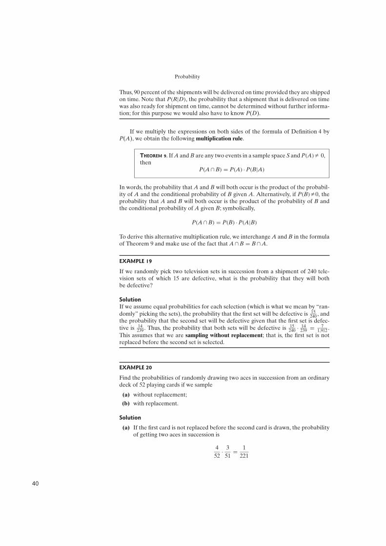
Probability
Thus, 90 percent of the shipments will be delivered on time provided they are shippedon time. Note that P(R|D), the probability that a shipment that is delivered on timewas also ready for shipment on time, cannot be determined without further informa-tion; for this purpose we would also have to know P(D).
If we multiply the expressions on both sides of the formula of Definition 4 byP(A), we obtain the following multiplication rule.
THEOREM 9. If A and B are any two events in a sample space S and P(A)Z 0,then
P(A ∩ B) = P(A) · P(B|A)
In words, the probability that A and B will both occur is the product of the probabil-ity of A and the conditional probability of B given A. Alternatively, if P(B)Z 0, theprobability that A and B will both occur is the product of the probability of B andthe conditional probability of A given B; symbolically,
P(A ∩ B) = P(B) · P(A|B)
To derive this alternative multiplication rule, we interchange A and B in the formulaof Theorem 9 and make use of the fact that A ∩ B = B ∩ A.
EXAMPLE 19
If we randomly pick two television sets in succession from a shipment of 240 tele-vision sets of which 15 are defective, what is the probability that they will bothbe defective?
Solution
If we assume equal probabilities for each selection (which is what we mean by “ran-domly” picking the sets), the probability that the first set will be defective is 15
240 , andthe probability that the second set will be defective given that the first set is defec-tive is 14
239 . Thus, the probability that both sets will be defective is 15240 · 14
239 = 71,912 .
This assumes that we are sampling without replacement; that is, the first set is notreplaced before the second set is selected.
EXAMPLE 20
Find the probabilities of randomly drawing two aces in succession from an ordinarydeck of 52 playing cards if we sample
(a) without replacement;
(b) with replacement.
Solution
(a) If the first card is not replaced before the second card is drawn, the probabilityof getting two aces in succession is
4
52·
3
51=
1
221
'%

Probability
(b) If the first card is replaced before the second card is drawn, the correspondingprobability is
4
52·
4
52=
1
169
In the situations described in the two preceding examples there is a definitetemporal order between the two events A and B. In general, this need not be thecase when we write P(A|B) or P(B|A). For instance, we could ask for the probabil-ity that the first card drawn was an ace given that the second card drawn (withoutreplacement) is an ace—the answer would also be 3
51 .Theorem 9 can easily be generalized so that it applies to more than two events;
for instance, for three events we have the following theorem.
THEOREM 10. If A, B, and C are any three events in a sample space S suchthat P(A ∩ B)Z 0, then
P(A ∩ B ∩ C) = P(A) · P(B|A) · P(C|A ∩ B)
Proof Writing A ∩ B ∩ C as (A ∩ B)∩ C and using the formula of Theo-rem 9 twice, we get
P(A ∩ B ∩ C) = P[(A ∩ B)∩ C]
= P(A ∩ B) · P(C|A ∩ B)
= P(A) · P(B|A) · P(C|A ∩ B)
EXAMPLE 21
A box of fuses contains 20 fuses, of which 5 are defective. If 3 of the fuses are selectedat random and removed from the box in succession without replacement, what is theprobability that all 3 fuses are defective?
Solution
If A is the event that the first fuse is defective, B is the event that the second fuseis defective, and C is the event that the third fuse is defective, then P(A) = 5
20 ,
P(B|A) = 419 , P(C|A ∩ B) = 3
18 , and substitution into the formula yields
P(A ∩ B ∩ C) =5
20·
4
19·
3
18
=1
114
Further generalization of Theorems 9 and 10 to k events is straightforward, andthe resulting formula can be proved by mathematical induction.
'&

Probability
7 Independent Events
Informally speaking, two events A and B are independent if the occurrence or nonoc-currence of either one does not affect the probability of the occurrence of the other.For instance, in the preceding example the selections would all have been indepen-dent had each fuse been replaced before the next one was selected; the probabilityof getting a defective fuse would have remained 5
20 .Symbolically, two events A and B are independent if P(B|A) = P(B) and
P(A|B) = P(A), and it can be shown that either of these equalities implies the otherwhen both of the conditional probabilities exist, that is, when neither P(A) nor P(B)equals zero (see Exercise 21).
Now, if we substitute P(B) for P(B|A) into the formula of Theorem 9, we get
P(A ∩ B) = P(A) · P(B|A)
= P(A) · P(B)
and we shall use this as our formal definition of independence.
DEFINITION 5. INDEPENDENCE. Two events A and B are independent if and only if
P(A ∩ B) = P(A) · P(B)
Reversing the steps, we can also show that Definition 5 implies the definition of inde-pendence that we gave earlier.
If two events are not independent, they are said to be dependent. In the deriva-tion of the formula of Definition 5, we assume that P(B|A) exists and, hence, thatP(A)Z 0. For mathematical convenience, we shall let the definition apply also whenP(A) = 0 and/or P(B) = 0.
EXAMPLE 22
A coin is tossed three times and the eight possible outcomes, HHH, HHT, HTH,THH, HTT, THT, TTH, and TTT, are assumed to be equally likely. If A is the eventthat a head occurs on each of the first two tosses, B is the event that a tail occurson the third toss, and C is the event that exactly two tails occur in the three tosses,show that
(a) events A and B are independent;
(b) events B and C are dependent.
Solution
Since
A = {HHH, HHT}
B = {HHT, HTT, THT, TTT}
C = {HTT, THT, TTH}
A ∩ B = {HHT}
B ∩ C = {HTT, THT}
'

Probability
the assumption that the eight possible outcomes are all equiprobable yieldsP(A) = 1
4 , P(B) = 12 , P(C) = 3
8 , P(A ∩ B) = 18 , and P(B ∩ C) = 1
4 .
(a) Since P(A) · P(B) = 14 · 1
2 = 18 = P(A ∩ B), events A and B are independent.
(b) Since P(B) · P(C) = 12 · 3
8 = 316 Z P(B ∩ C), events B and C are not inde-
pendent.
In connection with Definition 5, it can be shown that if A and B are independent,then so are A and B′, A′ and B, and A′ and B′. For instance, consider the followingtheorem.
THEOREM 11. If A and B are independent, then A and B′ are also indepen-dent.
Proof Since A = (A ∩ B)∪ (A ∩ B′), as the reader was asked to show inpart (a) of Exercise 3, A ∩ B and A ∩ B′ are mutually exclusive, and A andB are independent by assumption, we have
P(A) = P[(A ∩ B)∪ (A ∩ B′)]
= P(A ∩ B)+ P(A ∩ B′)
= P(A) · P(B)+ P(A ∩ B′)
It follows that
P(A ∩ B′) = P(A)− P(A) · P(B)
= P(A) · [1 − P(B)]
= P(A) · P(B′)
and hence that A and B′ are independent.
In Exercises 22 and 23 the reader will be asked to show that if A and B areindependent, then A′ and B are independent and so are A′ and B′, and if A and B
are dependent, then A and B′ are dependent.To extend the concept of independence to more than two events, let us make the
following definition.
DEFINITION 6. INDEPENDENCE OF MORE THAN TWO EVENTS. Events A1, A2, . . . , and
Ak are independent if and only if the probability of the intersections of any 2, 3,
. . . , or k of these events equals the product of their respective probabilities.
For three events A, B, and C, for example, independence requires that
P(A ∩ B) = P(A) · P(B)
P(A ∩ C) = P(A) · P(C)
P(B ∩ C) = P(B) · P(C)
'$

Probability
andP(A ∩ B ∩ C) = P(A) · P(B) · P(C)
It is of interest to note that three or more events can be pairwise independent
without being independent.
EXAMPLE 23
Figure 8 shows a Venn diagram with probabilities assigned to its various regions.Verify that A and B are independent, A and C are independent, and B and C areindependent, but A, B, and C are not independent.
Solution
As can be seen from the diagram, P(A) = P(B) = P(C) = 12 , P(A ∩ B) =
P(A ∩ C) = P(B ∩ C) = 14 , and P(A ∩ B ∩ C) = 1
4 . Thus,
P(A) · P(B) =1
4= P(A ∩ B)
P(A) · P(C) =1
4= P(A ∩ C)
P(B) · P(C) =1
4= P(B ∩ C)
but
P(A) · P(B) · P(C) =1
8Z P(A ∩ B ∩ C)
A B
C
14
14
14
14
Figure 8. Venn diagram for Example 23.
Incidentally, the preceding example can be given a “real” interpretation by con-sidering a large room that has three separate switches controlling the ceiling lights.These lights will be on when all three switches are “up” and hence also when oneof the switches is “up” and the other two are “down.” If A is the event that the firstswitch is “up,” B is the event that the second switch is “up,” and C is the event thatthe third switch is “up,” the Venn diagram of Figure 8 shows a possible set of prob-abilities associated with the switches being “up” or “down” when the ceiling lightsare on.
''

Probability
It can also happen that P(A ∩ B ∩ C) = P(A) · P(B) · P(C) without A, B, and C
being pairwise independent—this the reader will be asked to verify in Exercise 24.Of course, if we are given that certain events are independent, the probability
that they will all occur is simply the product of their respective probabilities.
EXAMPLE 24
Find the probabilities of getting
(a) three heads in three random tosses of a balanced coin;
(b) four sixes and then another number in five random rolls of a balanced die.
Solution
(a) The probability of a head on each toss is1
2and the three outcomes are inde-
pendent. Thus we can multiply, obtaining
1
2·
1
2·
1
2=
1
8
(b) The probability of a six on each toss is1
6; thus the probability of tossing a
number other than 6 is5
6. Inasmuch as the tosses are independent, we can
multiply the respective probabilities to obtain
1
6·
1
6·
1
6·
1
6·
5
6=
5
7, 776
8 Bayes’ Theorem
In many situations the outcome of an experiment depends on what happens in var-ious intermediate stages. The following is a simple example in which there is oneintermediate stage consisting of two alternatives:
EXAMPLE 25
The completion of a construction job may be delayed because of a strike. The prob-abilities are 0.60 that there will be a strike, 0.85 that the construction job will becompleted on time if there is no strike, and 0.35 that the construction job will becompleted on time if there is a strike. What is the probability that the constructionjob will be completed on time?
Solution
If A is the event that the construction job will be completed on time and B is theevent that there will be a strike, we are given P(B) = 0.60, P(A|B′) = 0.85, andP(A|B) = 0.35. Making use of the formula of part (a) of Exercise 3, the fact that A ∩B and A ∩ B′ are mutually exclusive, and the alternative form of the multiplicationrule, we can write
P(A) = P[(A ∩ B)∪ (A ∩ B′)]
= P(A ∩ B)+ P(A ∩ B′)
= P(B) · P(A|B)+ P(B′) · P(A|B′)
'(
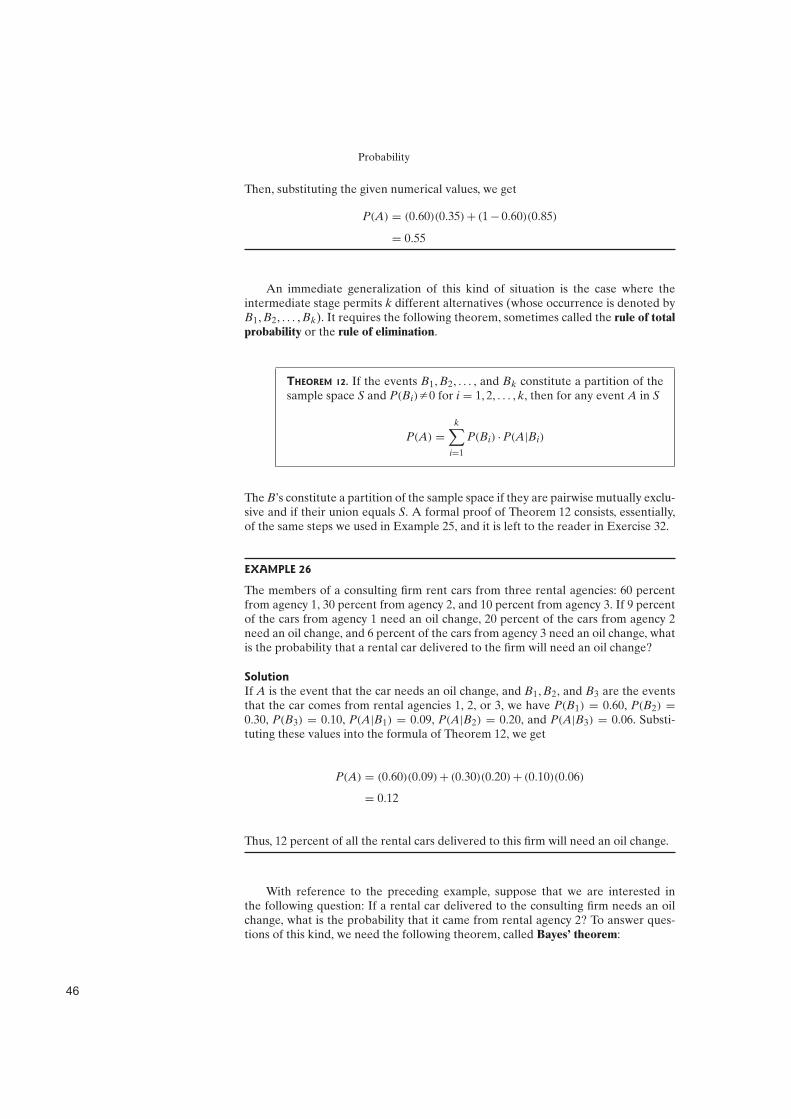
Probability
Then, substituting the given numerical values, we get
P(A) = (0.60)(0.35)+ (1 − 0.60)(0.85)
= 0.55
An immediate generalization of this kind of situation is the case where theintermediate stage permits k different alternatives (whose occurrence is denoted byB1, B2, . . . , Bk). It requires the following theorem, sometimes called the rule of total
probability or the rule of elimination.
THEOREM 12. If the events B1, B2, . . . , and Bk constitute a partition of thesample space S and P(Bi)Z 0 for i = 1, 2, . . . , k, then for any event A in S
P(A) =k∑
i=1
P(Bi) · P(A|Bi)
The B’s constitute a partition of the sample space if they are pairwise mutually exclu-sive and if their union equals S. A formal proof of Theorem 12 consists, essentially,of the same steps we used in Example 25, and it is left to the reader in Exercise 32.
EXAMPLE 26
The members of a consulting firm rent cars from three rental agencies: 60 percentfrom agency 1, 30 percent from agency 2, and 10 percent from agency 3. If 9 percentof the cars from agency 1 need an oil change, 20 percent of the cars from agency 2need an oil change, and 6 percent of the cars from agency 3 need an oil change, whatis the probability that a rental car delivered to the firm will need an oil change?
Solution
If A is the event that the car needs an oil change, and B1, B2, and B3 are the eventsthat the car comes from rental agencies 1, 2, or 3, we have P(B1) = 0.60, P(B2) =0.30, P(B3) = 0.10, P(A|B1) = 0.09, P(A|B2) = 0.20, and P(A|B3) = 0.06. Substi-tuting these values into the formula of Theorem 12, we get
P(A) = (0.60)(0.09)+ (0.30)(0.20)+ (0.10)(0.06)
= 0.12
Thus, 12 percent of all the rental cars delivered to this firm will need an oil change.
With reference to the preceding example, suppose that we are interested inthe following question: If a rental car delivered to the consulting firm needs an oilchange, what is the probability that it came from rental agency 2? To answer ques-tions of this kind, we need the following theorem, called Bayes’ theorem:
')

Probability
THEOREM 13. If B1, B2, . . . , Bk constitute a partition of the sample spaceS and P(Bi)Z 0 for i = 1, 2, . . . , k, then for any event A in S such thatP(A)Z 0
P(Br|A) =P(Br) · P(A|Br)
k∑
i=1
P(Bi) · P(A|Bi)
for r = 1, 2, . . . , k.
In words, the probability that event A was reached via the rth branchof the tree diagram of Figure 9, given that it was reached via one ofits k branches, is the ratio of the probability associated with the rthbranch to the sum of the probabilities associated with all k branches ofthe tree.
Proof Writing P(Br|A) =P(A ∩ Br)
P(A)in accordance with the definition
of conditional probability, we have only to substitute P(Br) · P(A|Br) forP(A ∩ Br) and the formula of Theorem 12 for P(A).
P(B 1)
P(B2)
P(Bk)
B1
B2
etc. etc.
A
A
A
P(B1) ? P(AuB1)P(AuB1)
P(AuB2)
P(AuBk)
P(B2) ? P(AuB2)
P(Bk) ? P(AuBk)Bk
Figure 9. Tree diagram for Bayes’ theorem.
EXAMPLE 27
With reference to Example 26, if a rental car delivered to the consulting firm needsan oil change, what is the probability that it came from rental agency 2?
Solution
Substituting the probabilities on the previous page into the formula of Theorem 13,we get
P(B2|A) =(0.30)(0.20)
(0.60)(0.09)+ (0.30)(0.20)+ (0.10)(0.06)
=0.060
0.120
= 0.5
Observe that although only 30 percent of the cars delivered to the firm come fromagency 2, 50 percent of those requiring an oil change come from that agency.
'!

Probability
EXAMPLE 28
A rare but serious disease, D, has been found in 0.01 percent of a certain population.A test has been developed that will be positive, p, for 98 percent of those who havethe disease and be positive for only 3 percent of those who do not have the disease.Find the probability that a person tested as positive does not have the disease.
Solution
Let D and p represent the events that a person randomly selected from the givenpopulation, respectively, does not have the disease and is found negative for the dis-ease by the test. Substituting the given probabilities into the formula of Theorem 13,we get
P(D|p) =P(D)P(p|D)
P(D)P(p|D)+ P(D)P(p|D)=
0.9999 · 0.03
0.0001 · 0.98 + 0.9999 · 0.03= 0.997
This example demonstrates the near impossibility of finding a test for a rare diseasethat does not have an unacceptably high probability of false positives.
Although Bayes’ theorem follows from the postulates of probability and thedefinition of conditional probability, it has been the subject of extensive controversy.There can be no question about the validity of Bayes’ theorem, but considerablearguments have been raised about the assignment of the prior probabilities P(Bi).Also, a good deal of mysticism surrounds Bayes’ theorem because it entails a “back-ward,” or “inverse,” sort of reasoning, that is, reasoning “from effect to cause.” Forinstance, in Example 27, needing an oil change is the effect and coming from agency2 of is a possible cause.
Exercises
17. Show that the postulates of probability are satisfiedby conditional probabilities. In other words, show that ifP(B)Z 0, then(a) P(A|B) G 0;
(b) P(B|B) = 1;
(c) P(A1 ∪ A2 ∪ . . . |B) = P(A1|B)+ P(A2|B)+ · · · forany sequence of mutually exclusive events A1, A2, . . ..
18. Show by means of numerical examples that P(B|A)+P(B|A′)(a) may be equal to 1;
(b) need not be equal to 1.
19. Duplicating the method of proof of Theorem 10,show that P(A∩B∩C∩D) = P(A) ·P(B|A) ·P(C|A∩B) ·P(D|A ∩ B ∩ C) provided that P(A ∩ B ∩ C)Z 0.
20. Given three events A, B, and C such thatP(A ∩ B ∩ C)Z 0 and P(C|A ∩ B) = P(C|B), show thatP(A|B ∩ C) = P(A|B).
21. Show that if P(B|A) = P(B) and P(B)Z 0, thenP(A|B) = P(A).
22. Show that if events A and B are independent, then(a) events A′ and B are independent;
(b) events A′ and B′ are independent.
23. Show that if events A and B are dependent, thenevents A and B′ are dependent.
24. Refer to Figure 10 to show that P(A ∩ B ∩ C) =P(A) · P(B) · P(C) does not necessarily imply that A, B,and C are all pairwise independent.
25. Refer to Figure 10 to show that if A is independentof B and A is independent of C, then B is not necessarilyindependent of C.
26. Refer to Figure 10 to show that if A is independent ofB and A is independent of C, then A is not necessarilyindependent of B ∪ C.
27. If events A, B, and C are independent, show that(a) A and B ∩ C are independent;
(b) A and B ∪ C are independent.
28. If P(A|B)< P(A), prove that P(B|A)< P(B).
'"

Probability
A B
C
0.06 0.18
0.06 0.14
0.24
0.24
0.06
0.02
Figure 10. Diagram for Exercises 24, 25, and 26.
29. If A1, A2, . . . , An are independent events, prove that
P(A1 ∪ A2 ∪ · · · ∪ An) = 1 −{1 − P(A1)} ·
{1 − P(A2)} . . . {1 − P(An)}
30. Show that 2k − k − 1 conditions must be satisfied fork events to be independent.
31. For any event A, show that A and ∅ areindependent.
32. Prove Theorem 12 by making use of the followinggeneralization of the distributive law given in part (b) ofExercise 1:
A∩ (B1∪B2∪· · ·∪Bk)=(A∩B1)∪(A∩B2)∪· · ·∪(A∩Bk)
33. Suppose that a die has n sides numbered i = 1,2, . . . , n. Assume that the probability of it coming up onthe side numbered i is the same for each value of i. The dieis rolled n times (assume independence) and a “match” isdefined to be the occurrence of side i on the ith roll. Provethat the probability of at least one match is given by
1 −(
n − 1
n
)n
= 1 −(
1 −1
n
)n
34. Show that P(A ∪ B)Ú 1 − P(A′)− P(B′) for any twoevents A and B defined in the sample space S. (Hint: UseVenn diagrams.)
9 The Theory in Practice
The word “probability” is a part of everyday language, but it is difficult to define thisword without using the word “probable” or its synonym “likely” in the definition.∗
To illustrate, Webster’s Third New International Dictionary defines “probability” as“the quality or state of being probable.” If the concept of probability is to be usedin mathematics and scientific applications, we require a more exact, less circular,definition.
The postulates of probability given in Section 4 satisfy this criterion. Togetherwith the rules given in Section 5, this definition lends itself to calculations of proba-bilities that “make sense” and that can be verified experimentally. The entire theoryof statistics is based on the notion of probability. It seems remarkable that the entirestructure of probability and, therefore of statistics, can be built on the relativelystraightforward foundation given in this chapter.
Probabilities were first considered in games of chance, or gambling. Players ofvarious games of chance observed that there seemed to be “rules” that governedthe roll of dice or the results of spinning a roulette wheel. Some of them went as faras to postulate some of these rules entirely on the basis of experience. But differ-ences arose among gamblers about probabilities, and they brought their questionsto the noted mathematicians of their day. With this motivation, the modern theoryof probability began to be developed.
Motivated by problems associated with games of chance, the theory of prob-ability first was developed under the assumption of equal likelihood, expressed inTheorem 2. Under this assumption one only had to count the number of “success-ful” outcomes and divide by the total number of “possible” outcomes to arrive atthe probability of an event.
The assumption of equal likelihood fails when we attempt, for example, to findthe probability that a trifecta at the race track will pay off. Here, the different horseshave different probabilities of winning, and we are forced to rely on a differentmethod of evaluating probabilities. It is common to take into account the various
∗From MERRIAM-WEBSTER’S COLLEGIATE DICTIONARY, ELEVENTH EDITION. Copyright 2012by Merriam-Webster, Incorporated (www.Merriam-Webster.com). Reprinted with permission.
'#
Probability
horses’ records in previous races, calculating each horse’s probability of winning bydividing its number of wins by the number of starts. This idea gives rise to the fre-
quency interpretation of probabilities, which interprets the probability of an event tobe the proportion of times the event has occurred in a long series of repeated exper-iments. Application of the frequency interpretation requires a well-documented his-tory of the outcomes of an event over a large number of experimental trials. In theabsence of such a history, a series of experiments can be planned and their resultsobserved. For example, the probability that a lot of manufactured items will have atmost three defectives is estimated to be 0.90 if, in 90 percent of many previous lotsproduced to the same specifications by the same process, the number of defectiveswas three or less.
A more recently employed method of calculating probabilities is called the sub-
jective method. Here, a personal or subjective assessment is made of the probabilityof an event which is difficult or impossible to estimate in any other way. For exam-ple, the probability that the major stock market indexes will go up in a given futureperiod of time cannot be estimated very well using the frequency interpretationbecause economic and world conditions rarely replicate themselves very closely. Asanother example, juries use this method when determining the guilt or innocence ofa defendant “beyond a reasonable doubt.” Subjective probabilities should be usedonly when all other methods fail, and then only with a high level of skepticism.
An important application of probability theory relates to the theory of reliabil-
ity. The reliability of a component or system can be defined as follows.
DEFINITION 7. RELIABILITY. The reliability of a product is the probability that it
will function within specified limits for a specified period of time under specified
environmental conditions.
Thus, the reliability of a “standard equipment” automobile tire is close to 1 for 10,000miles of operation on a passenger car traveling within the speed limits on pavedroads, but it is close to zero for even short distances at the Indianapolis “500.”
The reliability of a system of components can be calculated from the reliabil-ities of the individual components if the system consists entirely of componentsconnected in series, or in parallel, or both. A series system is one in which all com-ponents are so interrelated that the entire system will fail if any one (or more) of itscomponents fails. A parallel system will fail only if all its components fail. An exam-ple of a series system is a string of Christmas lights connected electrically “in series.”If one bulb fails, the entire string will fail to light. Parallel systems are sometimescalled “redundant” systems. For example, if the hydraulic system on a commercialaircraft that lowers the landing wheels fails, they may be lowered manually with acrank.
We shall assume that the components connected in a series system are indepen-dent; that is, the performance of one part does not affect the reliability of the others.Under this assumption, the reliability of a parallel system is given by an extension ofDefinition 5. Thus, we have the following theorem.
THEOREM 14. The reliability of a series system consisting of n independentcomponents is given by
Rs =n∏
i=1
Ri
where Ri is the reliability of the ith component.
Proof The proof follows immediately by iterating in Definition 5.
(%

Probability
Theorem 14 vividly demonstrates the effect of increased complexity on reliability.For example, if a series system has 5 components, each with a reliability of 0.970,the reliability of the entire system is only (0.970)5 = 0.859. If the system complexitywere increased so it now has 10 such components, the reliability would be reducedto (0.970)10 = 0.738.
One way to improve the reliability of a series system is to introduce parallelredundancy by replacing some or all of its components by several components con-nected in parallel. If a system consists of n independent components connected inparallel, it will fail to function only if all components fail. Thus, for the ith com-ponent, the probability of failure is Fi = 1 − Ri, called the “unreliability” of thecomponent. Again applying Definition 5, we obtain the following theorem.
THEOREM 15. The reliability of a parallel system consisting of n indepen-dent components is given by
Rp = 1 −n∏
i=1
(1 − Ri)
Proof The proof of this theorem is identical to that of Theorem 14, with(1 − Ri) replacing Ri.
EXAMPLE 29
Consider the system diagramed in Figure 11, which consists of eight componentshaving the reliabilities shown in the figure. Find the reliability of the system.
Solution
The parallel subsystem C, D, E can be replaced by an equivalent component, C′
having the reliability 1 − (1 − 0.70)3 = 0.973. Likewise, F, G can be replaced by F ′
having the reliability 1 − (1 − 0.75)2 = 0.9375. Thus, the system is reduced to the par-allel system A, B, C′, F ′, H, having the reliability (0.95)(0.99)(0.973)(0.9375)(0.90) =0.772.
BA
0.95 0.99
C
0.70
D
0.70
E
0.70
H
0.90
F
0.75
G
0.75
Figure 11. Combination of series and parallel systems.
(&

Probability
Applied Exercises SECS. 1–3
35. If S = {1, 2, 3, 4, 5, 6, 7, 8, 9}, A = {1, 3, 5, 7}, B ={6, 7, 8, 9}, C = {2, 4, 8}, and D = {1, 5, 9}, list the elementsof the subsets of S corresponding to the following events:
(a) A′ ∩ B; (b) (A′ ∩ B)∩ C; (c) B′ ∪ C;
(d) (B′ ∪ C)∩ D; (e) A′ ∩ C; (f) (A′ ∩ C)∩ D.
36. An electronics firm plans to build a research labora-tory in Southern California, and its management has todecide between sites in Los Angeles, San Diego, LongBeach, Pasadena, Santa Barbara, Anaheim, Santa Mon-ica, and Westwood. If A represents the event that theywill choose a site in San Diego or Santa Barbara, B repre-sents the event that they will choose a site in San Diego orLong Beach, C represents the event that they will choosea site in Santa Barbara or Anaheim, and D representsthe event that they will choose a site in Los Angeles orSanta Barbara, list the elements of each of the followingsubsets of the sample space, which consists of the eightsite selections:
(a) A′; (b) D′; (c) C ∩ D;
(d) B ∩ C; (e) B ∪ C; (f) A ∪ B;
(g) C ∪ D; (h) (B ∪ C)′; (i) B′ ∩ C′.
37. Among the eight cars that a dealer has in his show-room, Car 1 is new and has air-conditioning, power steer-ing, and bucket seats; Car 2 is one year old and has air-conditioning, but neither power steering nor bucket seats;Car 3 is two years old and has air-conditioning and powersteering, but no bucket seats; Car 4 is three years oldand has air-conditioning, but neither power steering norbucket seats; Car 5 is new and has no air-conditioning, nopower steering, and no bucket seats; Car 6 is one yearold and has power steering, but neither air-conditioningnor bucket seats; Car 7 is two years old and has no air-conditioning, no power steering, and no bucket seats; andCar 8 is three years old, and has no air-conditioning, buthas power steering as well as bucket seats. If a customerbuys one of these cars and the event that he chooses anew car, for example, is represented by the set {Car 1,Car 5}, indicate similarly the sets that represent theevents that(a) he chooses a car without air-conditioning;
(b) he chooses a car without power steering;
(c) he chooses a car with bucket seats;
(d) he chooses a car that is either two or three years old.
38. With reference to Exercise 37, state in words whatkind of car the customer will choose, if his choice isgiven by(a) the complement of the set of part (a);
(b) the union of the sets of parts (b) and (c);
(c) the intersection of the sets of parts (c) and (d);
(d) the intersection of parts (b) and (c) of this exercise.
39. If Ms. Brown buys one of the houses advertised forsale in a Seattle newspaper (on a given Sunday), T is theevent that the house has three or more baths, U is theevent that it has a fireplace, V is the event that it costsmore than $200,000, and W is the event that it is new,describe (in words) each of the following events:
(a) T ′; (b) U′; (c) V′;
(d) W′; (e) T ∩ U; (f) T ∩ V;
(g) U′ ∩ V; (h) V ∪ W; (i) V′ ∪ W;
(j) T ∪ U; (k) T ∪ V; (l) V ∩ W.
40. A resort hotel has two station wagons, which it usesto shuttle its guests to and from the airport. If the largerof the two station wagons can carry five passengers andthe smaller can carry four passengers, the point (0, 3)represents the event that at a given moment the largerstation wagon is empty while the smaller one has threepassengers, the point (4, 2) represents the event that atthe given moment the larger station wagon has four pas-sengers while the smaller one has two passengers, . . . ,draw a figure showing the 30 points of the correspondingsample space. Also, if E stands for the event that at leastone of the station wagons is empty, F stands for the eventthat together they carry two, four, or six passengers, andG stands for the event that each carries the same num-ber of passengers, list the points of the sample space thatcorrespond to each of the following events:
(a) E; (b) F; (c) G;
(d) E ∪ F; (e) E ∩ F; (f) F ∪ G;
(g) E ∪ F ′; (h) E ∩ G′; (i) F ′ ∩ E′.
41. A coin is tossed once. Then, if it comes up heads, adie is thrown once; if the coin comes up tails, it is tossedtwice more. Using the notation in which (H, 2), for exam-ple, denotes the event that the coin comes up heads andthen the die comes up 2, and (T, T, T) denotes the eventthat the coin comes up tails three times in a row, list(a) the 10 elements of the sample space S;
(b) the elements of S corresponding to event A thatexactly one head occurs;
(c) the elements of S corresponding to event B that atleast two tails occur or a number greater than 4 occurs.
42. An electronic game contains three componentsarranged in the series–parallel circuit shown in Figure 12.At any given time, each component may or may not beoperative, and the game will operate only if there is acontinuous circuit from P to Q. Let A be the eventthat the game will operate; let B be the event that
(

Probability
P Q
y
x
z
Figure 12. Diagram for Exercise 42.
the game will operate though component x is not oper-ative; and let C be the event that the game will operatethough component y is not operative. Using the notationin which (0, 0, 1), for example, denotes that component zis operative but components x and y are not,(a) list the elements of the sample space S and also theelements of S corresponding to events A, B, and C;
(b) determine which pairs of events, A and B, A and C, orB and C, are mutually exclusive.
43. An experiment consists of rolling a die until a 3appears. Describe the sample space and determine(a) how many elements of the sample space correspondto the event that the 3 appears on the kth roll of the die;
(b) how many elements of the sample space correspondto the event that the 3 appears not later than the kth rollof the die.
44. Express symbolically the sample space S that consistsof all the points (x, y) on or in the circle of radius 3 cen-tered at the point (2, −3).
45. If S = {x|0 < x < 10}, M = {x|3 < x F 8}, and N ={x|5 < x < 10}, find
(a) M ∪ N; (b) M ∩ N;
(c) M ∩ N′; (d) M′ ∪ N.
46. In Figure 13, L is the event that a driver has liabilityinsurance and C is the event that she has collision insur-ance. Express in words what events are represented byregions 1, 2, 3, and 4.
2 1 3
4
L C
Figure 13. Venn diagram for Exercise 46.
47. With reference to Exercise 46 and Figure 13, whatevents are represented by(a) regions 1 and 2 together;
(b) regions 2 and 4 together;
(c) regions 1, 2, and 3 together;
(d) regions 2, 3, and 4 together?
48. In Figure 14, E, T, and N are the events that a carbrought to a garage needs an engine overhaul, transmis-sion repairs, or new tires. Express in words the eventsrepresented by(a) region 1;
(b) region 3;
(c) region 7;
(d) regions 1 and 4 together;
(e) regions 2 and 5 together;
(f) regions 3, 5, 6, and 8 together.
7 2
1
6 8
5
4 3
E T
N
Figure 14. Venn diagram for Exercise 48.
49. With reference to Exercise 48 and Figure 14, list theregion or combinations of regions representing the eventsthat a car brought to the garage needs(a) transmission repairs, but neither an engine overhaulnor new tires;
(b) an engine overhaul and transmission repairs;
(c) transmission repairs or new tires, but not anengine overhaul;
(d) new tires.
50. A market research organization claims that, among500 shoppers interviewed, 308 regularly buy Product X,266 regularly buy Product Y, 103 regularly buy both, and59 buy neither on a regular basis. Using a Venn diagramand filling in the number of shoppers associated with thevarious regions, check whether the results of this studyshould be questioned.
51. In a group of 200 college students, 138 are enrolledin a course in psychology, 115 are enrolled in a course insociology, and 91 are enrolled in both. How many of thesestudents are not enrolled in either course? (Hint: Draw asuitable Venn diagram and fill in the numbers associatedwith the various regions.)
52. Among 120 visitors to Disneyland, 74 stayed for atleast 3 hours, 86 spent at least $20, 64 went on the Mat-terhorn ride, 60 stayed for at least 3 hours and spent at
($

Probability
least $20, 52 stayed for at least 3 hours and went on theMatterhorn ride, 54 spent at least $20 and went on theMatterhorn ride, and 48 stayed for at least 3 hours, spentat least $20, and went on the Matterhorn ride. Drawing aVenn diagram with three circles (like that of Figure 4) andfilling in the numbers associated with the various regions,find how many of the 120 visitors to Disneyland(a) stayed for at least 3 hours, spent at least $20, but didnot go on the Matterhorn ride;
(b) went on the Matterhorn ride, but stayed less than 3hours and spent less than $20;
(c) stayed less than 3 hours, spent at least $20, but did notgo on the Matterhorn ride.
SECS. 4–5
53. An experiment has five possible outcomes, A, B, C, D,and E, that are mutually exclusive. Check whether the fol-lowing assignments of probabilities are permissible andexplain your answers:(a) P(A) = 0.20, P(B) = 0.20, P(C) = 0.20, P(D) = 0.20,and P(E) = 0.20;
(b) P(A) = 0.21, P(B) = 0.26, P(C) = 0.58, P(D) = 0.01,and P(E) = 0.06;
(c) P(A) = 0.18, P(B) = 0.19, P(C) = 0.20, P(D) = 0.21,and P(E) = 0.22;
(d) P(A) = 0.10, P(B) = 0.30, P(C) = 0.10, P(D) = 0.60,and P(E) = −0.10;
(e) P(A) = 0.23, P(B) = 0.12, P(C) = 0.05, P(D) = 0.50,and P(E) = 0.08.
54. If A and B are mutually exclusive, P(A) = 0.37, andP(B) = 0.44, find
(a) P(A′); (b) P(B′); (c) P(A ∪ B);
(d) P(A ∩ B); (e) P(A ∩ B′); (f) P(A′ ∩ B′).
55. Explain why there must be a mistake in each of thefollowing statements:(a) The probability that Jean will pass the bar examina-tion is 0.66 and the probability that she will not pass is−0.34.
(b) The probability that the home team will win anupcoming football game is 0.77, the probability that it willtie the game is 0.08, and the probability that it will win ortie the game is 0.95.
(c) The probabilities that a secretary will make 0, 1, 2, 3, 4,or 5 or more mistakes in typing a report are, respectively,0.12, 0.25, 0.36, 0.14, 0.09, and 0.07.
(d) The probabilities that a bank will get 0, 1, 2, or 3 ormore bad checks on any given day are, respectively, 0.08,0.21, 0.29, and 0.40.
56. The probabilities that the serviceability of a newX-ray machine will be rated very difficult, difficult, aver-age, easy, or very easy are, respectively, 0.12, 0.17, 0.34,0.29, and 0.08. Find the probabilities that the serviceabil-ity of the machine will be rated
(a) difficult or very difficult;
(b) neither very difficult nor very easy;
(c) average or worse;
(d) average or better.
57. Suppose that each of the 30 points of the sample spaceof Exercise 40 is assigned the probability 1
30 . Find theprobabilities that at a given moment(a) at least one of the station wagons is empty;
(b) each of the two station wagons carries the same num-ber of passengers;
(c) the larger station wagon carries more passengers thanthe smaller station wagon;
(d) together they carry at least six passengers.
58. A hat contains 20 white slips of paper numbered from1 through 20, 10 red slips of paper numbered from 1through 10, 40 yellow slips of paper numbered from 1through 40, and 10 blue slips of paper numbered from 1through 10. If these 80 slips of paper are thoroughly shuf-fled so that each slip has the same probability of beingdrawn, find the probabilities of drawing a slip of paperthat is(a) blue or white;
(b) numbered 1, 2, 3, 4, or 5;
(c) red or yellow and also numbered 1, 2, 3, or 4;
(d) numbered 5, 15, 25, or 35;
(e) white and numbered higher than 12 or yellow andnumbered higher than 26.
59. A police department needs new tires for its patrolcars and the probabilities are 0.15, 0.24, 0.03, 0.28, 0.22,and 0.08, respectively, that it will buy Uniroyal tires,Goodyear tires, Michelin tires, General tires, Goodrichtires, or Armstrong tires. Find the probabilities that itwill buy(a) Goodyear or Goodrich tires;
(b) Uniroyal, Michelin, or Goodrich tires;
(c) Michelin or Armstrong tires;
(d) Uniroyal, Michelin, General, or Goodrich tires.
60. Two cards are randomly drawn from a deck of 52playing cards. Find the probability that both cards will begreater than 3 and less than 8.
61. Four candidates are seeking a vacancy on a schoolboard. If A is twice as likely to be elected as B, and Band C are given about the same chance of being elected,while C is twice as likely to be elected as D, what are theprobabilities that(a) C will win;
(b) A will not win?
62. In a poker game, five cards are dealt at random froman ordinary deck of 52 playing cards. Find the probabili-ties of getting
('

Probability
(a) two pairs (any two distinct face values occurringexactly twice);
(b) four of a kind (four cards of equal face value).
63. In a game of Yahtzee, five balanced dice are rolledsimultaneously. Find the probabilities of getting(a) two pairs;
(b) three of a kind;
(c) a full house (three of a kind and a pair);
(d) four of a kind.
64. Explain on the basis of the various rules ofExercises 5 through 9 why there is a mistake in each ofthe following statements:(a) The probability that it will rain is 0.67, and the proba-bility that it will rain or snow is 0.55.
(b) The probability that a student will get a passing gradein English is 0.82, and the probability that she will get apassing grade in English and French is 0.86.
(c) The probability that a person visiting the San DiegoZoo will see the giraffes is 0.72, the probability that hewill see the bears is 0.84, and the probability that he willsee both is 0.52.
65. Among the 78 doctors on the staff of a hospital, 64carry malpractice insurance, 36 are surgeons, and 34 ofthe surgeons carry malpractice insurance. If one of thesedoctors is chosen by lot to represent the hospital staff atan A.M.A. convention (that is, each doctor has a proba-bility of 1
78 of being selected), what is the probability thatthe one chosen is not a surgeon and does not carry mal-practice insurance?
66. A line segment of length l is divided by a pointselected at random within the segment. What is the prob-ability that it will divide the line segment in a ratio greaterthan 1:2? What is the probability that it will divide thesegment exactly in half?
67. A right triangle has the legs 3 and 4 units, respectively.Find the probability that a line segment, drawn at randomparallel to the hypotenuse and contained entirely in thetriangle, will divide the triangle so that the area betweenthe line and the vertex opposite the hypotenuse will equalat least half the area of the triangle.
68. For married couples living in a certain suburb, theprobability that the husband will vote in a school boardelection is 0.21, the probability that the wife will vote inthe election is 0.28, and the probability that they will bothvote is 0.15. What is the probability that at least one ofthem will vote?
69. Given P(A) = 0.59, P(B) = 0.30, and P(A ∩ B) =0.21, find
(a) P(A ∪ B); (b) P(A ∩ B′);
(c) P(A′ ∪ B′); (d) P(A′ ∩ B′).
70. At Roanoke College it is known that 13 of the stu-
dents live off campus. It is also known that 59 of the stu-
dents are from within the state of Virginia and that 34
of the students are from out of state or live on campus.What is the probability that a student selected at ran-dom from Roanoke College is from out of state and liveson campus?
71. A biology professor has two graduate assistants help-ing her with her research. The probability that the olderof the two assistants will be absent on any given day is0.08, the probability that the younger of the two will beabsent on any given day is 0.05, and the probability thatthey will both be absent on any given day is 0.02. Find theprobabilities that(a) either or both of the graduate assistants will be absenton any given day;
(b) at least one of the two graduate assistants will not beabsent on any given day;
(c) only one of the two graduate assistants will be absenton any given day.
72. Suppose that if a person visits Disneyland, the prob-ability that he will go on the Jungle Cruise is 0.74, theprobability that he will ride the Monorail is 0.70, the prob-ability that he will go on the Matterhorn ride is 0.62, theprobability that he will go on the Jungle Cruise and ridethe Monorail is 0.52, the probability that he will go on theJungle Cruise as well as the Matterhorn ride is 0.46, theprobability that he will ride the Monorail and go on theMatterhorn ride is 0.44, and the probability that he willgo on all three of these rides is 0.34. What is the proba-bility that a person visiting Disneyland will go on at leastone of these three rides?
73. Suppose that if a person travels to Europe for thefirst time, the probability that he will see London is 0.70,the probability that he will see Paris is 0.64, the proba-bility that he will see Rome is 0.58, the probability thathe will see Amsterdam is 0.58, the probability that hewill see London and Paris is 0.45, the probability that hewill see London and Rome is 0.42, the probability thathe will see London and Amsterdam is 0.41, the probabil-ity that he will see Paris and Rome is 0.35, the probabilitythat he will see Paris and Amsterdam is 0.39, the proba-bility that he will see Rome and Amsterdam is 0.32, theprobability that he will see London, Paris, and Rome is0.23, the probability that he will see London, Paris, andAmsterdam is 0.26, the probability that he will see Lon-don, Rome, and Amsterdam is 0.21, the probability thathe will see Paris, Rome, and Amsterdam is 0.20, and theprobability that he will see all four of these cities is 0.12.What is the probability that a person traveling to Europefor the first time will see at least one of these four cities?(Hint: Use the formula of Exercise 13.)
((

Probability
74. Use the formula of Exercise 15 to convert each of thefollowing odds to probabilities:(a) If three eggs are randomly chosen from a carton of 12eggs of which 3 are cracked, the odds are 34 to 21 that atleast one of them will be cracked.
(b) If a person has eight $1 bills, five $5 bills, and one $20bill, and randomly selects three of them, the odds are 11to 2 that they will not all be $1 bills.
(c) If we arbitrarily arrange the letters in the word “nest,”the odds are 5 to 1 that we will not get a meaningful wordin the English language.
75. Use the definition of “odds” given in Exercise 15 toconvert each of the following probabilities to odds:(a) The probability that the last digit of a car’s licenseplate is a 2, 3, 4, 5, 6, or 7 is 6
10 .
(b) The probability of getting at least two heads in fourflips of a balanced coin is 11
16 .
(c) The probability of rolling “7 or 11” with a pair of bal-anced dice is 2
9 .
SECS. 6–8
76. There are 90 applicants for a job with the news depart-ment of a television station. Some of them are collegegraduates and some are not; some of them have at leastthree years’ experience and some have not, with the exactbreakdown being
Collegegraduates
Notcollegegraduates
At least three years’ experience 18 9
Less than three years’ experience 36 27
If the order in which the applicants are interviewed bythe station manager is random, G is the event that thefirst applicant interviewed is a college graduate, and T isthe event that the first applicant interviewed has at leastthree years’ experience, determine each of the followingprobabilities directly from the entries and the row andcolumn totals of the table:
(a) P(G); (b) P(T ′); (c) P(G ∩ T);
(d) P(G′ ∩ T ′); (e) P(T|G); (f) P(G′|T ′).
77. Use the results of Exercise 76 to verify that
(a) P(T|G) = P(G∩T)P(G)
;
(b) P(G′|T ′) = P(G′∩T′)P(T′) .
78. With reference to Exercise 65, what is the probabilitythat the doctor chosen to represent the hospital staff atthe convention carries malpractice insurance given thathe or she is a surgeon?
79. With reference to Exercise 68, what is the probabilitythat a husband will vote in the election given that his wifeis going to vote?
80. With reference to Exercise 70, what is the probabilitythat one of the students will be living on campus giventhat he or she is from out of state?
81. A bin contains 100 balls, of which 25 are red, 40 arewhite, and 35 are black. If two balls are selected from thebin without replacement, what is the probability that onewill be red and one will be white?
82. If subjective probabilities are determined by themethod suggested in Exercise 16, the third postulate ofprobability may not be satisfied. However, proponentsof the subjective probability concept usually impose thispostulate as a consistency criterion; in other words, theyregard subjective probabilities that do not satisfy the pos-tulate as inconsistent.(a) A high school principal feels that the odds are 7 to 5against her getting a $1,000 raise and 11 to 1 against hergetting a $2,000 raise. Furthermore, she feels that it is aneven-money bet that she will get one of these raises orthe other. Discuss the consistency of the correspondingsubjective probabilities.
(b) Asked about his political future, a party officialreplies that the odds are 2 to 1 that he will not run forthe House of Representatives and 4 to 1 that he will notrun for the Senate. Furthermore, he feels that the oddsare 7 to 5 that he will run for one or the other. Are thecorresponding probabilities consistent?
83. If we let x = the number of spots facing up when apair of dice is cast, then we can use the sample space S2 ofExample 2 to describe the outcomes of the experiment.(a) Find the probability of each outcome in S2.
(b) Verify that the sum of these probabilities is 1.
84. There are two Porsches in a road race in Italy, and areporter feels that the odds against their winning are 3to 1 and 5 to 3. To be consistent (see Exercise 82), whatodds should the reporter assign to the event that eithercar will win?
85. Using a computer program that can generate randomintegers on the interval (0, 9) with equal probabilities,generate 1,000 such integers and use the frequency inter-pretation to estimate the probability that such a randomlychosen integer will have a value less than 1.
86. Using the method of Exercise 85, generate a secondset of 1,000 random integers on (0, 9). Estimate the prob-ability that A: an integer selected at random from the firstset will be less than 1 or B: an integer selected at randomfrom the second set will be less than 1(a) using the frequency interpretation of probabilities;
(b) using Theorem 7 and P(A ∩ B) = 181 .
()

Probability
87. It is felt that the probabilities are 0.20, 0.40, 0.30,and 0.10 that the basketball teams of four universities,T, U, V, and W, will win their conference championship.If university U is placed on probation and declaredineligible for the championship, what is the probabil-ity that university T will win the conference champi-onship?
88. With reference to Exercise 72, find the probabilitiesthat a person who visits Disneyland will(a) ride the Monorail given that he will go on the Jun-gle Cruise;
(b) go on the Matterhorn ride given that he will go on theJungle Cruise and ride the Monorail;
(c) not go on the Jungle Cruise given that he will ride theMonorail and/or go on the Matterhorn ride;
(d) go on the Matterhorn ride and the Jungle Cruise giventhat he will not ride the Monorail.
(Hint: Draw a Venn diagram and fill in the probabilitiesassociated with the various regions.)
89. Crates of eggs are inspected for blood clots by ran-domly removing three eggs in succession and examiningtheir contents. If all three eggs are good, the crate isshipped; otherwise it is rejected. What is the probabilitythat a crate will be shipped if it contains 120 eggs, of which10 have blood clots?
90. The probability of surviving a certain transplant oper-ation is 0.55. If a patient survives the operation, the prob-ability that his or her body will reject the transplant withina month is 0.20. What is the probability of surviving bothof these critical stages?
91. Suppose that in Vancouver, B.C., the probability thata rainy fall day is followed by a rainy day is 0.80 and theprobability that a sunny fall day is followed by a rainyday is 0.60. Find the probabilities that a rainy fall day isfollowed by(a) a rainy day, a sunny day, and another rainy day;
(b) two sunny days and then a rainy day;
(c) two rainy days and then two sunny days;
(d) rain two days later.
[Hint: In part (c) use the formula of Exercise 19.]
92. Use the formula of Exercise 19 to find the probabilityof randomly choosing (without replacement) four healthyguinea pigs from a cage containing 20 guinea pigs, ofwhich 15 are healthy and 5 are diseased.
93. A sharpshooter hits a target with probability 0.75.Assuming independence, find the probabilities of getting(a) a hit followed by two misses;
(b) two hits and a miss in any order.
94. A balanced die is tossed twice. If A is the event thatan even number comes up on the first toss, B is the eventthat an even number comes up on the second toss, and Cis the event that both tosses result in the same number,are the events A, B, and C(a) pairwise independent;
(b) independent?
95. A shipment of 1,000 parts contains 1 percent defectiveparts. Find the probability that(a) the first four parts chosen arbitrarily for inspection arenondefective;
(b) the first defective part found will be on the fourthinspection.
96. A coin is loaded so that the probabilities of heads andtails are 0.52 and 0.48, respectively. If the coin is tossedthree times, what are the probabilities of getting(a) all heads;
(b) two tails and a head in that order?
97. If 5 of a company’s 10 delivery trucks do not meetemission standards and 3 of them are chosen for inspec-tion, what is the probability that none of the trucks cho-sen will meet emission standards?
98. Medical records show that one out of 10 persons ina certain town has a thyroid deficiency. If 12 persons inthis town are randomly chosen and tested, what is theprobability that at least one of them will have a thy-roid deficiency?
99. If a person randomly picks 4 of the 15 gold coins adealer has in stock, and 6 of the coins are counterfeits,what is the probability that the coins picked will all becounterfeits?
100. A department store that bills its charge-account cus-tomers once a month has found that if a customer payspromptly one month, the probability is 0.90 that he orshe will also pay promptly the next month; however, ifa customer does not pay promptly one month, the prob-ability that he or she will pay promptly the next month isonly 0.40. (Assume that the probability of paying or notpaying on any given month depends only on the outcomeof the previous month.)(a) What is the probability that a customer who payspromptly one month will also pay promptly the nextthree months?
(b) What is the probability that a customer who does notpay promptly one month will also not pay promptly thenext two months and then make a prompt payment themonth after that?
101. With reference to Figure 15, verify that events A, B,C, and D are independent. Note that the region repre-senting A consists of two circles, and so do the regionsrepresenting B and C.
(!

Probability
A B
C
A
D
B
C
118
118
118
118
118
118
118
19
19
19
19
118
136
136
136
136
Figure 15. Diagram for Exercise 101.
102. At an electronics plant, it is known from past expe-rience that the probability is 0.84 that a new worker whohas attended the company’s training program will meetthe production quota, and that the corresponding prob-ability is 0.49 for a new worker who has not attendedthe company’s training program. If 70 percent of all newworkers attend the training program, what is the proba-bility that a new worker will meet the production quota?
103. It is known from experience that in a certain indus-try 60 percent of all labor–management disputes are overwages, 15 percent are over working conditions, and 25percent are over fringe issues. Also, 45 percent of thedisputes over wages are resolved without strikes, 70 per-cent of the disputes over working conditions are resolvedwithout strikes, and 40 percent of the disputes over fringeissues are resolved without strikes. What is the probabil-ity that a labor–management dispute in this industry willbe resolved without a strike?
104. In a T-maze, a rat is given food if it turns left and anelectric shock if it turns right. On the first trial there isa 50–50 chance that a rat will turn either way; then, if itreceives food on the first trial, the probability is 0.68 thatit will turn left on the next trial, and if it receives a shockon the first trial, the probability is 0.84 that it will turn lefton the next trial. What is the probability that a rat willturn left on the second trial?
105. With reference to Exercise 103, what is the probabil-ity that if a labor–management dispute in this industry isresolved without a strike, it was over wages?
106. The probability that a one-car accident is due tofaulty brakes is 0.04, the probability that a one-car acci-dent is correctly attributed to faulty brakes is 0.82, and
the probability that a one-car accident is incorrectlyattributed to faulty brakes is 0.03. What is the probabil-ity that(a) a one-car accident will be attributed to faulty brakes;
(b) a one-car accident attributed to faulty brakes wasactually due to faulty brakes?
107. With reference to Example 25, suppose that we dis-cover later that the job was completed on time. What isthe probability that there had been a strike?
108. In a certain community, 8 percent of all adults over50 have diabetes. If a health service in this communitycorrectly diagnoses 95 percent of all persons with dia-betes as having the disease and incorrectly diagnoses 2percent of all persons without diabetes as having the dis-ease, find the probabilities that(a) the community health service will diagnose an adultover 50 as having diabetes;
(b) a person over 50 diagnosed by the health service ashaving diabetes actually has the disease.
109. An explosion at a construction site could haveoccurred as the result of static electricity, malfunctioningof equipment, carelessness, or sabotage. Interviews withconstruction engineers analyzing the risks involved ledto the estimates that such an explosion would occur withprobability 0.25 as a result of static electricity, 0.20 as aresult of malfunctioning of equipment, 0.40 as a result ofcarelessness, and 0.75 as a result of sabotage. It is alsofelt that the prior probabilities of the four causes of theexplosion are 0.20, 0.40, 0.25, and 0.15. Based on all thisinformation, what is(a) the most likely cause of the explosion;
(b) the least likely cause of the explosion?
("

Probability
110. A mail-order house employs three stock clerks, U,V, and W, who pull items from shelves and assemblethem for subsequent verification and packaging. U makesa mistake in an order (gets a wrong item or the wrongquantity) one time in a hundred, V makes a mistake inan order five times in a hundred, and W makes a mistakein an order three times in a hundred. If U, V, and W fill,respectively, 30, 40, and 30 percent of all orders, what arethe probabilities that(a) a mistake will be made in an order;
(b) if a mistake is made in an order, the order was filledby U;
(c) if a mistake is made in an order, the order was filledby V?
111. An art dealer receives a shipment of five old paint-ings from abroad, and, on the basis of past experience,she feels that the probabilities are, respectively, 0.76, 0.09,0.02, 0.01, 0.02, and 0.10 that 0, 1, 2, 3, 4, or all 5 of themare forgeries. Since the cost of authentication is fairlyhigh, she decides to select one of the five paintings at ran-dom and send it away for authentication. If it turns outthat this painting is a forgery, what probability should shenow assign to the possibility that all the other paintingsare also forgeries?
112. To get answers to sensitive questions, we sometimesuse a method called the randomized response technique.Suppose, for instance, that we want to determine whatpercentage of the students at a large university smokemarijuana. We construct 20 flash cards, write “I smokemarijuana at least once a week” on 12 of the cards, where12 is an arbitrary choice, and “I do not smoke marijuanaat least once a week” on the others. Then, we let each stu-dent (in the sample interviewed) select one of the 20 cardsat random and respond “yes” or “no” without divulgingthe question.(a) Establish a relationship between P(Y), the probabil-ity that a student will give a “yes” response, and P(M),the probability that a student randomly selected at thatuniversity smokes marijuana at least once a week.
(b) If 106 of 250 students answered “yes” under theseconditions, use the result of part (a) and 106
250 as an esti-mate of P(Y) to estimate P(M).
SEC. 9
113. A series system consists of three components, eachhaving the reliability 0.95, and three components, eachhaving the reliability 0.99. Find the reliability of thesystem.
114. Find the reliability of a series systems having fivecomponents with reliabilities 0.995, 0.990, 0.992, 0.995,and 0.998, respectively.
115. What must be the reliability of each component in aseries system consisting of six components that must havea system reliability of 0.95?
116. Referring to Exercise 115, suppose now that thereare 10 components, and the system reliability must be0.90.
117. Suppose a system consists of four components, con-nected in parallel, having the reliabilities 0.8, 0.7, 0.7, and0.65, respectively. Find the system reliability.
118. Referring to Exercise 117, suppose now that the sys-tem has five components with reliabilities 0.85, 0.80, 0.65,0.60, and 0.70, respectively. Find the system reliability.
119. A system consists of two components having the reli-abilities 0.95 and 0.90, connected in series to two parallelsubsystems, the first containing four components, eachhaving the reliability 0.60, and the second containing twocomponents, each having the reliability 0.75. Find the sys-tem reliability.
120. A series system consists of two components havingthe reliabilities 0.98 and 0.99, respectively, connected to aparallel subsystem containing five components having thereliabilities 0.75, 0.60, 0.65, 0.70, and 0.60, respectively.Find the system reliability.
References
Among the numerous textbooks on probability theorypublished in recent years, one of the most popular is
Feller, W., An Introduction to Probability Theory and ItsApplications, Vol. I, 3rd ed. New York: John Wiley &Sons, Inc., 1968.
More elementary treatments may be found in
Barr, D. R., and Zehna, P. W., Probability: ModelingUncertainty. Reading, Mass.: Addison-Wesley Publish-ing Company, Inc., 1983,
Draper, N. R., and Lawrence, W. E., Probability: AnIntroductory Course. Chicago: Markam PublishingCompany, 1970,
Freund, J. E., Introduction to Probability. New York:Dover Publications, Inc., 1993 Reprint,
Goldberg, S., Probability—An Introduction. Mineola,N.Y.: Dover Publications, Inc. (republication of 1960edition),
Hodges, J. L., and Lehmann, E. L., Elements of FiniteProbability. San Francisco: Holden Day, Inc.,1965,
Nosal, M., Basic Probability and Applications. Philadel-phia: W. B. Saunders Company, 1977.
More advanced treatments are given in many texts,for instance,
(#
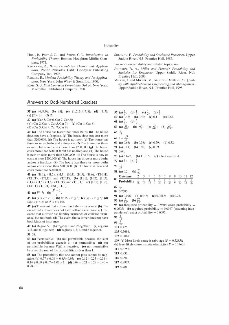
Probability
Hoel, P., Port, S. C., and Stone, C. J., Introduction toProbability Theory. Boston: Houghton Mifflin Com-pany, 1971,
Khazanie, R., Basic Probability Theory and Applica-tions. Pacific Palisades, Calif.: Goodyear PublishingCompany, Inc., 1976,
Parzen, E., Modern Probability Theory and Its Applica-tions. New York: John Wiley & Sons, Inc., 1960,
Ross, S., A First Course in Probability, 3rd ed. New York:Macmillan Publishing Company, 1988.
Solomon, F., Probability and Stochastic Processes. UpperSaddle River, N.J.: Prentice Hall, 1987.
For more on reliability and related topics, see
Johnson, R. A., Miller and Freund’s Probability andStatistics for Engineers. Upper Saddle River, N.J.:Prentice Hall, 2000,
Miller, I. and Miller, M., Statistical Methods for Qual-ity with Applications to Engineering and Management.Upper Saddle River, N.J.: Prentice Hall, 1995.
Answers to Odd-Numbered Exercises
35 (a) {6, 8, 9}; (b) {8}; (c) {1, 2, 3, 4, 5, 8}; (d) {1, 5};(e) {2, 4, 8}; (f) Ø.
37 (a) {Car 5, Car 6, Car 7, Car 8};(b) {Car 2, Car 4, Car 5, Car 7}; (c) {Car 1, Car 8};(d) {Car 3, Car 4, Car 7, Car 8}.39 (a) The house has fewer than three baths. (b) The housedoes not have a fireplace. (c) The house does not cost morethan $200,000. (d) The house is not new. (e) The house hasthree or more baths and a fireplace. (f) The house has threeor more baths and costs more than $200,000. (g) The housecosts more than $200,000 but has no fireplace. (h) The houseis new or costs more than $200,000. (i) The house is new orcosts at most $200,000. (j) The house has three or more bathsand/or a fireplace. (k) The house has three or more bathsand/or costs more than $200,000. (l) The house is new andcosts more than $200,000.
41 (a) (H,1), (H,2), (H,3), (H,4), (H,5), (H,6), (T,H,H),(T,H,T), (T,T,H), and (T,T,T); (b) (H,1), (H,2), (H,3),(H,4), (H,5), (H,6), (T,H,T), and (T,T,H); (c) (H,5), (H,6),(T,H,T), (T,T,H), and (T,T,T).
43 (a) 5k−1; (b)5k − 1
4.
45 (a) (x|3 < x < 10); (b) (x|15 < x ≤ 8); (c) (x|3 < x ≤ 5); (d)
(x|0 < x ≤ 3) or (5 < x < 10).
47 (a) The event that a driver has liability insurance. (b) Theevent that a driver does not have collision insurance. (c) Theevent that a driver has liability insurance or collision insur-ance, but not both. (d) The event that a driver does not haveboth kinds of insurance.
49 (a) Region 5; (b) regions 1 and 2 together; (c) regions3, 5, and 6 together; (d) regions 1, 3, 4, and 6 together.
51 38.
53 (a) Permissible; (b) not permissible because the sumof the probabilities exceeds 1; (c) permissible; (d) notpermissible because P(E) is negative; (e) not permissiblebecause the sum of the probabilities is less than 1.
55 (a) The probability that she cannot pass cannot be neg-ative. (b) 0.77 + 0.08 = 0.85 Z 0.95; (c) 0.12 + 0.25 + 0.36 +0.14 + 0.09 + 0.07=1.03 > 1; (d) 0.08 + 0.21 + 0.29 + 0.40=0.98 < 1.
57 (a) 13 ; (b) 1
6 ; (c) 12 ; (d) 1
3 .
59 (a) 0.46; (b) 0.40; (c) 0.11 (d) 0.68.
61 (a) 29 ; (b) 5
9 .
63 (a) 25108 ; (b) 25
162 ; (c) 25648 ; (d) 25
1296 .
65 213 .
67 1 −√
22 .
69 (a) 0.68; (b) 0.38; (c) 0.79; (d) 0.32.
71 (a) 0.11; (b) 0.98; (c) 0.09.
73 0.94.
75 (a) 3 to 2; (b) 11 to 5; (c) 7 to 2 against it.
77 (a) 13 ; (b) 3
7 .
79 1528 .
81 (a) 0.2; (b) 2099 .
83Outcome 2 3 4 5 6 7 8 9 10 11 12
Probability 136
118
112
19
536
16
536
19
112
118
136
87 13 .
89 0.7685.
91 (a) 0.096; (b) 0.048; (c) 0.0512; (d) 0.76.
93 (a) 364 ; (b) 27
64 .
95 (a) Required probability = 0.9606; exact probability =0.9605; (b) required probability = 0.0097 (assuming inde-pendence); exact probability = 0.0097.
97 112 .
99 191 .
103 0.475.
105 0.5684.
107 0.3818.
109 (a) Most likely cause is sabotage (P = 0.3285);(b) least likely cause is static electricity (P = 0.1460).
111 0.6757.
113 0.832.
115 0.991.
117 0.9937.
119 0.781.
)%
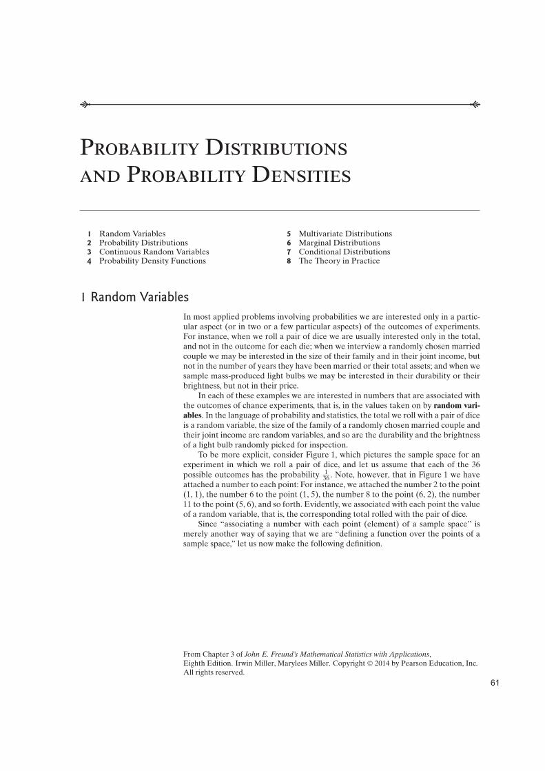
Probability Distributions
and Probability Densities
1 Random Variables2 Probability Distributions3 Continuous Random Variables4 Probability Density Functions
5 Multivariate Distributions6 Marginal Distributions7 Conditional Distributions8 The Theory in Practice
1 Random Variables
In most applied problems involving probabilities we are interested only in a partic-ular aspect (or in two or a few particular aspects) of the outcomes of experiments.For instance, when we roll a pair of dice we are usually interested only in the total,and not in the outcome for each die; when we interview a randomly chosen marriedcouple we may be interested in the size of their family and in their joint income, butnot in the number of years they have been married or their total assets; and when wesample mass-produced light bulbs we may be interested in their durability or theirbrightness, but not in their price.
In each of these examples we are interested in numbers that are associated withthe outcomes of chance experiments, that is, in the values taken on by random vari-
ables. In the language of probability and statistics, the total we roll with a pair of diceis a random variable, the size of the family of a randomly chosen married couple andtheir joint income are random variables, and so are the durability and the brightnessof a light bulb randomly picked for inspection.
To be more explicit, consider Figure 1, which pictures the sample space for anexperiment in which we roll a pair of dice, and let us assume that each of the 36possible outcomes has the probability 1
36 . Note, however, that in Figure 1 we haveattached a number to each point: For instance, we attached the number 2 to the point(1, 1), the number 6 to the point (1, 5), the number 8 to the point (6, 2), the number11 to the point (5, 6), and so forth. Evidently, we associated with each point the valueof a random variable, that is, the corresponding total rolled with the pair of dice.
Since “associating a number with each point (element) of a sample space” ismerely another way of saying that we are “defining a function over the points of asample space,” let us now make the following definition.
From Chapter 3 of John E. Freund’s Mathematical Statistics with Applications,Eighth Edition. Irwin Miller, Marylees Miller. Copyright 2014 by Pearson Education, Inc.All rights reserved.
)&

Probability Distributions and Probability Densities
12 3 4 5 6 7
3 4 5 6 7 8
4 5 6 7 8 9
5 6 7 8 9 10
6 7 8 9 10 11
7 8 9 10 11 12
1
2
3
4
5
6
2 3 4 5 6Red die
Greendie
Figure 1. The total number of points rolled with a pair of dice.
DEFINITION 1. RANDOM VARIABLE. If S is a sample space with a probability measure
and X is a real-valued function defined over the elements of S, then X is called a
random variable.†
In this chapter we shall denote random variables by capital letters and their valuesby the corresponding lowercase letters; for instance, we shall write x to denote avalue of the random variable X.
With reference to the preceding example and Figure 1, observe that the randomvariable X takes on the value 9, and we write X = 9 for the subset
{(6, 3), (5, 4), (4, 5), (3, 6)}
of the sample space S. Thus, X = 9 is to be interpreted as the set of elements of S
for which the total is 9 and, more generally, X = x is to be interpreted as the set ofelements of the sample space for which the random variable X takes on the value x.This may seem confusing, but it reminds one of mathematicians who say “f (x) is afunction of x” instead of “f (x) is the value of a function at x.”
EXAMPLE 1
Two socks are selected at random and removed in succession from a drawer contain-ing five brown socks and three green socks. List the elements of the sample space, thecorresponding probabilities, and the corresponding values w of the random variableW, where W is the number of brown socks selected.
†Instead of “random variable,” the terms “chance variable,” “stochastic variable,” and “variate” are also used insome books.
!

Probability Distributions and Probability Densities
Solution
If B and G stand for brown and green, the probabilities for BB, BG, GB, and GG
are, respectively, 58 ·
47 =
514 , 5
8 ·37 =
1556 , 3
8 ·57 =
1556 , and 3
8 ·27 =
328 , and the results are
shown in the following table:
Element of
sample space Probability w
BB5
142
BG15
561
GB15
561
GG3
280
Also, we can write P(W = 2) = 514 , for example, for the probability of the event that
the random variable W will take on the value 2.
EXAMPLE 2
A balanced coin is tossed four times. List the elements of the sample space that arepresumed to be equally likely, as this is what we mean by a coin being balanced, andthe corresponding values x of the random variable X, the total number of heads.
Solution
If H and T stand for heads and tails, the results are as shown in the following table:
Element of
sample space Probability x
HHHH1
164
HHHT1
163
HHTH1
163
HTHH1
163
THHH1
163
HHTT1
162
HTHT1
162
"
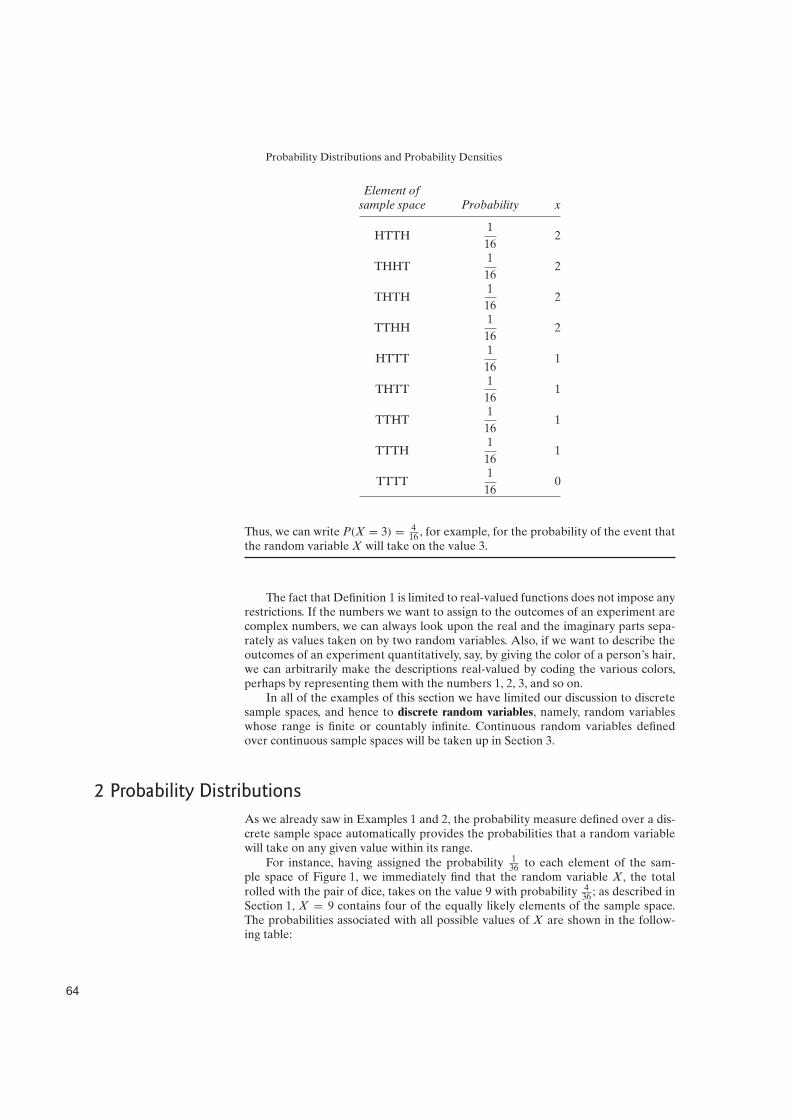
Probability Distributions and Probability Densities
Element of
sample space Probability x
HTTH1
162
THHT1
162
THTH1
162
TTHH1
162
HTTT1
161
THTT1
161
TTHT1
161
TTTH1
161
TTTT1
160
Thus, we can write P(X = 3) = 416 , for example, for the probability of the event that
the random variable X will take on the value 3.
The fact that Definition 1 is limited to real-valued functions does not impose anyrestrictions. If the numbers we want to assign to the outcomes of an experiment arecomplex numbers, we can always look upon the real and the imaginary parts sepa-rately as values taken on by two random variables. Also, if we want to describe theoutcomes of an experiment quantitatively, say, by giving the color of a person’s hair,we can arbitrarily make the descriptions real-valued by coding the various colors,perhaps by representing them with the numbers 1, 2, 3, and so on.
In all of the examples of this section we have limited our discussion to discretesample spaces, and hence to discrete random variables, namely, random variableswhose range is finite or countably infinite. Continuous random variables definedover continuous sample spaces will be taken up in Section 3.
2 Probability Distributions
As we already saw in Examples 1 and 2, the probability measure defined over a dis-crete sample space automatically provides the probabilities that a random variablewill take on any given value within its range.
For instance, having assigned the probability 136 to each element of the sam-
ple space of Figure 1, we immediately find that the random variable X, the totalrolled with the pair of dice, takes on the value 9 with probability 4
36 ; as described inSection 1, X = 9 contains four of the equally likely elements of the sample space.The probabilities associated with all possible values of X are shown in the follow-ing table:
#

Probability Distributions and Probability Densities
x P(X = x)
21
36
32
36
43
36
54
36
65
36
76
36
85
36
94
36
103
36
112
36
121
36
Instead of displaying the probabilities associated with the values of a randomvariable in a table, as we did in the preceding illustration, it is usually preferable togive a formula, that is, to express the probabilities by means of a function such thatits values, f (x), equal P(X = x) for each x within the range of the random variableX. For instance, for the total rolled with a pair of dice we could write
f (x) =6− |x− 7|
36for x = 2, 3, . . . , 12
as can easily be verified by substitution. Clearly,
f (2) =6− |2− 7|
36=
6− 5
36=
1
36
f (3) =6− |3− 7|
36=
6− 4
36=
2
36. . . . . . . . . . . . . . . . . . . . .
f (12) =6− |12− 7|
36=
6− 5
36=
1
36
and all these values agree with the ones shown in the preceding table.
DEFINITION 2. PROBABILITY DISTRIBUTION. If X is a discrete random variable, the
function given by f(x) = P(X = x) for each x within the range of X is called the
probability distribution of X.
$

Probability Distributions and Probability Densities
Based on the postulates of probability, we obtain the following theorem.
THEOREM 1. A function can serve as the probability distribution of a dis-crete random variable X if and only if its values, f (x), satisfy the conditions
1. f (x) G 0 for each value within its domain;
2.∑
xf (x) = 1, where the summation extends over all the values within
its domain.
EXAMPLE 3
Find a formula for the probability distribution of the total number of heads obtainedin four tosses of a balanced coin.
Solution
Based on the probabilities in the table, we find that P(X = 0) = 116 , P(X = 1) =
416 , P(X = 2) = 6
16 , P(X = 3) = 416 , and P(X = 4) = 1
16 . Observing that thenumerators of these five fractions, 1, 4, 6, 4, and 1, are the binomial coefficients(
40
)
,
(
41
)
,
(
42
)
,
(
43
)
, and
(
44
)
, we find that the formula for the probability distri-
bution can be written as
f (x) =
(
4x
)
16for x = 0, 1, 2, 3, 4
EXAMPLE 4
Check whether the function given by
f (x) =x+ 2
25for x = 1, 2, 3, 4, 5
can serve as the probability distribution of a discrete random variable.
Solution
Substituting the different values of x, we get f (1) = 325 , f (2) = 4
25 , f (3) = 525 ,
f (4) = 625 , and f (5) = 7
25 . Since these values are all nonnegative, the first conditionof Theorem 1 is satisfied, and since
f (1)+ f (2)+ f (3)+ f (4)+ f (5) =3
25+
4
25+
5
25+
6
25+
7
25
= 1
the second condition of Theorem 1 is satisfied. Thus, the given function can serve asthe probability distribution of a random variable having the range {1, 2, 3, 4, 5}. Ofcourse, whether any given random variable actually has this probability distributionis an entirely different matter.
In some problems it is desirable to present probability distributions graphi-cally, and two kinds of graphical presentations used for this purpose are shown inFigures 2 and 3. The one shown in Figure 2, called a probability histogram, repre-sents the probability distribution of Example 3. The height of each rectangle equals

Probability Distributions and Probability Densities
0 1 2
Number of heads
3 4x
f (x)
616
416
116
Figure 2. Probability histogram.
0 1 2
Number of heads
3 4x
f (x)
616
416
116
Figure 3. Bar chart.
the probability that X takes on the value that corresponds to the midpoint of itsbase. By representing 0 with the interval from −0.5 to 0.5, 1 with the interval from0.5 to 1.5, . . ., and 4 with the interval from 3.5 to 4.5, we are, so to speak, “spreading”the values of the given discrete random variable over a continuous scale.
Since each rectangle of the probability histogram of Figure 2 has unit width, wecould have said that the areas of the rectangles, rather than their heights, equal the
%

Probability Distributions and Probability Densities
corresponding probabilities. There are certain advantages to identifying the areasof the rectangles with the probabilities, for instance, when we wish to approximatethe graph of a discrete probability distribution with a continuous curve. This can bedone even when the rectangles of a probability histogram do not all have unit widthby adjusting the heights of the rectangles or by modifying the vertical scale.
The graph of Figure 3 is called a bar chart, but it is also referred to as a his-togram. As in Figure 2, the height of each rectangle, or bar, equals the probability ofthe corresponding value of the random variable, but there is no pretense of havinga continuous horizontal scale. Sometimes, as shown in Figure 4, we use lines (rect-angles with no width) instead of the rectangles, but we still refer to the graphs asprobability histograms.
In this chapter, histograms and bar charts are used mainly in descriptive statis-tics to convey visually the information provided by a probability distribution or adistribution of actual data (see Section 8).
There are many problems in which it is of interest to know the probability thatthe value of a random variable is less than or equal to some real number x. Thus,let us write the probability that X takes on a value less than or equal to x as F(x) =P(X F x) and refer to this function defined for all real numbers x as the distribution
function, or the cumulative distribution, of X.
0 1 2
Number of heads
3 4x
f (x)
616
416
116
Figure 4. Probability histogram.
DEFINITION 3. DISTRIBUTION FUNCTION. If X is a discrete random variable, the func-
tion given by
F(x) = P(X ≤ x) =∑
t≤x
f (t) for −q< x<q
where f(t) is the value of the probability distribution of X at t, is called the distri-bution function, or the cumulative distribution of X.
&

Probability Distributions and Probability Densities
Based on the postulates of probability and some of their immediate consequences,we obtain the following theorem.
THEOREM 2. The values F(x) of the distribution function of a discrete ran-dom variable X satisfy the conditions
1. F(−q) = 0 and F(q) = 1;
2. if a<b, then F(a) F F(b) for any real numbers a and b.
If we are given the probability distribution of a discrete random variable, thecorresponding distribution function is generally easy to find.
EXAMPLE 5
Find the distribution function of the total number of heads obtained in four tossesof a balanced coin.
Solution
Given f (0) = 116 , f (1) = 4
16 , f (2) = 616 , f (3) = 4
16 , and f (4) = 116 from Example 3, it
follows that
F(0) = f (0) =1
16
F(1) = f (0)+ f (1) =5
16
F(2) = f (0)+ f (1)+ f (2) =11
16
F(3) = f (0)+ f (1)+ f (2)+ f (3) =15
16F(4) = f (0)+ f (1)+ f (2)+ f (3)+ f (4) = 1
Hence, the distribution function is given by
F(x) =
0 for x< 01
16for 0 F x< 1
5
16for 1 F x< 2
11
16for 2 F x< 3
15
16for 3 F x< 4
1 for x G 4
Observe that this distribution function is defined not only for the values taken onby the given random variable, but for all real numbers. For instance, we can writeF(1.7) = 5
16 and F(100) = 1, although the probabilities of getting “at most 1.7 heads”or “at most 100 heads” in four tosses of a balanced coin may not be of any realsignificance.
'

Probability Distributions and Probability Densities
EXAMPLE 6
Find the distribution function of the random variable W of Example 1 and plotits graph.
Solution
Based on the probabilities given in the table in Section 1, we can write f (0) =328 , f (1) = 15
56 +1556 =
1528 , and f (2) = 5
14 , so that
F(0) = f (0) =3
28
F(1) = f (0)+ f (1) =9
14
F(2) = f (0)+ f (1)+ f (2) = 1
Hence, the distribution function of W is given by
F(w) =
0 for w< 0
3
28for 0 F w< 1
9
14for 1 F w< 2
1 for w G 2
The graph of this distribution function, shown in Figure 5, was obtained by first plot-ting the points (w, F(w)) for w = 0, 1, and 2 and then completing the step functionas indicated. Note that at all points of discontinuity the distribution function takeson the greater of the two values, as indicated by the heavy dots in Figure 5.
Figure 5. Graph of the distribution function of Example 6.
%(

Probability Distributions and Probability Densities
We can also reverse the process illustrated in the two preceding examples, thatis, obtain values of the probability distribution of a random variable from its distri-bution function. To this end, we use the following result.
THEOREM 3. If the range of a random variable X consists of the values x1<
x2< x3< · · ·< xn, then f (x1) = F(x1) and
f (xi) = F(xi)−F(xi−1) for i = 2, 3, . . . , n
EXAMPLE 7
If the distribution function of X is given by
F(x) =
0 for x< 2
1
36for 2 F x< 3
3
36for 3 F x< 4
6
36for 4 F x< 5
10
36for 5 F x< 6
15
36for 6 F x< 7
21
36for 7 F x< 8
26
36for 8 F x< 9
30
36for 9 F x< 10
33
36for 10 F x< 11
35
36for 11 F x< 12
1 for x G 12
find the probability distribution of this random variable.
Solution
Making use of Theorem 3, we get f (2) = 136 , f (3) = 3
36 −136 = 2
36 , f (4) = 636 −
336 =
336 , f (5) = 10
36 −6
36 =436 , . . . , f (12) = 1− 35
36 =136 , and comparison with the
probabilities in the table in Section 2 reveals that the random variable with whichwe are concerned here is the total number of points rolled with a pair of dice.
In the remainder of this chapter we will be concerned with continuous ran-dom variables and their distributions and with problems relating to the simultaneousoccurrence of the values of two or more random variables.
%)

Probability Distributions and Probability Densities
Exercises
1. For each of the following, determine whether thegiven values can serve as the values of a probability dis-tribution of a random variable with the range x = 1, 2, 3,and 4:
(a) f (1) = 0.25, f (2) = 0.75, f (3) = 0.25, and f (4) =
−0.25;
(b) f (1) = 0.15, f (2) = 0.27, f (3) = 0.29, and f (4) = 0.29;
(c) f (1) =1
19, f (2) =
10
19, f (3) =
2
19, and f (4) =
5
19.
2. For each of the following, determine whether the givenfunction can serve as the probability distribution of a ran-dom variable with the given range:
(a) f (x) =x− 2
5for x = 1, 2, 3, 4, 5;
(b) f (x) =x2
30for x = 0, 1, 2, 3, 4;
(c) f (x) =1
5for x = 0, 1, 2, 3, 4, 5.
3. Verify that f (x) =2x
k(k+ 1)for x = 1, 2, 3, . . . , k can
serve as the probability distribution of a random variablewith the given range.
4. For each of the following, determine c so that the func-tion can serve as the probability distribution of a randomvariable with the given range:
(a) f (x) = cx for x = 1, 2, 3, 4, 5;
(b) f (x) = c
(
5
x
)
for x = 0, 1, 2, 3, 4, 5;
(c) f (x) = cx2 for x = 1, 2, 3, . . . , k;
(d) f (x) = c
(
1
4
)x
for x = 1, 2, 3, . . . .
5. For what values of k can
f (x) = (1−k)kx
serve as the values of the probability distribution of arandom variable with the countably infinite range x =0, 1, 2, . . .?
6. Show that there are no values of c such that
f (x) =c
x
can serve as the values of the probability distributionof a random variable with the countably infinite rangex = 1, 2, 3, . . . .
7. Construct a probability histogram for each of the fol-lowing probability distributions:
(a) f (x) =
2
x
4
3− x
6
3
for x = 0, 1, 2;
(b) f (x) =(
5
x
)(
1
5
)x (4
5
)5−x
for x = 0, 1, 2, 3, 4, 5.
8. Prove Theorem 2.
9. For each of the following, determine whether the givenvalues can serve as the values of a distribution function ofa random variable with the range x = 1, 2, 3, and 4:(a) F(1) = 0.3, F(2) = 0.5, F(3) = 0.8, and F(4) = 1.2;
(b) F(1) = 0.5, F(2) = 0.4, F(3) = 0.7, and F(4) = 1.0;
(c) F(1) = 0.25, F(2) = 0.61, F(3) = 0.83, andF(4) = 1.0.
10. Find the distribution function of the random variableof part (a) of Exercise 7 and plot its graph.
11. If X has the distribution function
F(x) =
0 for x< 1
1
3for 1 F x< 4
1
2for 4 F x< 6
5
6for 6 F x< 10
1 for x G 10
find(a) P(2<X F 6);
(b) P(X = 4);
(c) the probability distribution of X.
12. Find the distribution function of the random variablethat has the probability distribution
f (x) =x
15for x = 1, 2, 3, 4, 5
%!

Probability Distributions and Probability Densities
13. If X has the distribution function
F(x) =
0 for x<−1
1
4for −1 F x< 1
1
2for 1 F x< 3
3
4for 3 F x< 5
1 for x G 5
find
(a) P(X F 3); (b) P(X = 3); (c) P(X < 3);
(d) P(X G 1); (e) P(−0.4<X < 4); (f) P(X = 5).
14. With reference to Example 4, verify that the values ofthe distribution function are given by
F(x) =x2+ 5x
50
for x = 1, 2, 3, 4, and 5.
15. With reference to Theorem 3, verify that
(a) P(X > xi) = 1−F(xi) for i = 1, 2, 3, . . . , n;
(b) P(X G xi) = 1−F(xi−1) for i = 2, 3, . . . , n,
and P(X G x1) = 1.
3 Continuous Random Variables
In Section 1 we introduced the concept of a random variable as a real-valued func-tion defined over the points of a sample space with a probability measure, and inFigure 1 we illustrated this by assigning the total rolled with a pair of dice to eachof the 36 equally likely points of the sample space. In the continuous case, whererandom variables can take on values on a continuous scale, the procedure is verymuch the same. The outcomes of experiments are represented by the points on linesegments or lines, and the values of random variables are numbers appropriatelyassigned to the points by means of rules or equations. When the value of a ran-dom variable is given directly by a measurement or observation, we generally donot bother to distinguish between the value of the random variable (the measure-ment that we obtain) and the outcome of the experiment (the corresponding pointon the real axis). Thus, if an experiment consists of determining the actual content ofa 230-gram jar of instant coffee, the result itself, say, 225.3 grams, is the value of therandom variable with which we are concerned, and there is no real need to add thatthe sample space consists of a certain continuous interval of points on the positivereal axis.
The problem of defining probabilities in connection with continuous samplespaces and continuous random variables involves some complications. To illustrate,let us consider the following situation.
EXAMPLE 8
Suppose that we are concerned with the possibility that an accident will occur on afreeway that is 200 kilometers long and that we are interested in the probability thatit will occur at a given location, or perhaps on a given stretch of the road. The samplespace of this “experiment” consists of a continuum of points, those on the intervalfrom 0 to 200, and we shall assume, for the sake of argument, that the probability
that an accident will occur on any interval of length d isd
200, with d measured in
%"
Probability Distributions and Probability Densities
kilometers. Note that this assignment of probabilities is consistent with Postulates 1and 2. (Postulate 1 states that probability of an event is a nonnegative real number;that is, P(A)G 0 for any subset A of S but in Postulate 2 P(S) = 1.) The probabilities
d
200are all nonnegative and P(S) =
200
200= 1. So far this assignment of probabilities
applies only to intervals on the line segment from 0 to 200, but if we use Postulate 3(Postulate 3: If A1, A2, A3, . . . , is a finite or infinite sequence of mutually exclusiveevents of S, then P(A1 ∪A2 ∪A3 ∪ · · · ) = P(A1)+P(A2)+P(A3)+ · · · ), we canalso obtain probabilities for the union of any finite or countably infinite sequenceof nonoverlapping intervals. For instance, the probability that an accident will occuron either of two nonoverlapping intervals of length d1 and d2 is
d1+d2
200
and the probability that it will occur on any one of a countably infinite sequence ofnonoverlapping intervals of length d1, d2, d3, . . . is
d1+d2+d3+ · · ·200
With reference to Example 8, observe also that the probability of the accidentoccurring on a very short interval, say, an interval of 1 centimeter, is only 0.00000005,which is very small. As the length of the interval approaches zero, the probabilitythat an accident will occur on it also approaches zero; indeed, in the continuous casewe always assign zero probability to individual points. This does not mean that thecorresponding events cannot occur; after all, when an accident occurs on the 200-kilometer stretch of road, it has to occur at some point even though each point haszero probability.
4 Probability Density Functions
The way in which we assigned probabilities in Example 8 is very special, and it issimilar in nature to the way in which we assign equal probabilities to the six facesof a die, heads and tails, the 52 playing cards in a standard deck, and so forth.To treat the problem of associating probabilities with values of continuous ran-dom variables more generally, suppose that a bottler of soft drinks is concernedabout the actual amount of a soft drink that his bottling machine puts into16-ounce bottles. Evidently, the amount will vary somewhat from bottle to bottle;it is, in fact, a continuous random variable. However, if he rounds the amountsto the nearest tenth of an ounce, he will be dealing with a discrete random vari-able that has a probability distribution, and this probability distribution may bepictured as a histogram in which the probabilities are given by the areas of rect-angles, say, as in the diagram at the top of Figure 6. If he rounds the amounts tothe nearest hundredth of an ounce, he will again be dealing with a discrete randomvariable (a different one) that has a probability distribution, and this probabilitydistribution may be pictured as a probability histogram in which the probabilities
%#

Probability Distributions and Probability Densities
15.9
Amounts rounded to nearest tenth of an ounce
16.0 16.1
15.9 16.0 16.1
15.90
Amounts rounded to nearest hundredth of an ounce
16.00 16.10
Figure 6. Definition of probability in the continuous case.
are given by the areas of rectangles, say, as in the diagram in the middle ofFigure 6.
It should be apparent that if he rounds the amounts to the nearest thousandthof an ounce or to the nearest ten-thousandth of an ounce, the probability histogramsof the probability distributions of the corresponding discrete random variables willapproach the continuous curve shown in the diagram at the bottom of Figure 6,and the sum of the areas of the rectangles that represent the probability that theamount falls within any specified interval approaches the corresponding area underthe curve.
Indeed, the definition of probability in the continuous case presumes foreach random variable the existence of a function, called a probability density
function, such that areas under the curve give the probabilities associated with thecorresponding intervals along the horizontal axis. In other words, a probabilitydensity function, integrated from a to b (with a F b), gives the probability thatthe corresponding random variable will take on a value on the interval froma to b.
%$
Probability Distributions and Probability Densities
DEFINITION 4. PROBABILITY DENSITY FUNCTION. A function with values f(x), defined
over the set of all real numbers, is called a probability density function of the
continuous random variable X if and only if
P(a ≤ X ≤ b) =∫ b
a
f (x)dx
for any real constants a and b with a…b.
Probability density functions are also referred to, more briefly, as probability densi-
ties, density functions, densities, or p.d.f.’s.Note that f (c), the value of the probability density of X at c, does not give
P(X = c) as in the discrete case. In connection with continuous random variables,probabilities are always associated with intervals and P(X = c) = 0 for any realconstant c. This agrees with what we said on the previous page and it also followsdirectly from Definition 4 with a = b = c.
Because of this property, the value of a probability density function can bechanged for some of the values of a random variable without changing the prob-abilities, and this is why we said in Definition 4 that f (x) is the value of a probabilitydensity, not the probability density, of the random variable X at x. Also, in view ofthis property, it does not matter whether we include the endpoints of the intervalfrom a to b; symbolically, we have the following theorem.
THEOREM 4. If X is a continuous random variable and a and b are realconstants with a F b, then
P(a F X F b) = P(a F X <b) = P(a<X F b) = P(a<X <b)
Analogous to Theorem 1, let us now state the following properties of probabilitydensities, which again follow directly from the postulates of probability.
THEOREM 5. A function can serve as a probability density of a continuousrandom variable X if its values, f (x), satisfy the conditions†
1. f (x) G 0 for −q< x<q;
2.
∫
q
−qf (x)dx = 1.
EXAMPLE 9
If X has the probability density
f (x) =
{
k · e−3x for x> 0
0 elsewhere
find k and P(0.5 F X F 1).
†The conditions are not “if and only if” as in Theorem 1 because f (x) could be negative for some values ofthe random variable without affecting any of the probabilities. However, both conditions of Theorem 5 will besatisfied by nearly all the probability densities used in practice and studied in this text.
%
Probability Distributions and Probability Densities
Solution
To satisfy the second condition of Theorem 5, we must have
∫
q
−qf (x)dx =
∫
q
0k · e−3x dx = k · lim
t→q
e−3x
−3
∣
∣
∣
t
0=
k
3= 1
and it follows that k = 3. For the probability we get
P(0.5 F X F 1) =∫ 1
0.53e−3x dx = −e−3x
∣
∣
∣
1
0.5= −e−3+ e−1.5 = 0.173
Although the random variable of the preceding example cannot take on negativevalues, we artificially extended the domain of its probability density to include allthe real numbers. This is a practice we shall follow throughout this text.
As in the discrete case, there are many problems in which it is of interest toknow the probability that the value of a continuous random variable X is less thanor equal to some real number x. Thus, let us make the following definition analogousto Definition 3.
DEFINITION 5. DISTRIBUTION FUNCTION. If X is a continuous random variable and
the value of its probability density at t is f(t), then the function given by
F(x) = P(X ≤ x) =∫ x
−qf (t)dt for −q< x<q
is called the distribution function or the cumulative distribution function of X.
The properties of distribution functions given in Theorem 2 hold also for thecontinuous case; that is, F(−q) = 0, F(q) = 1, and F(a) F F(b) when a<b. Fur-thermore, based on Definition 5, we can state the following theorem.
THEOREM 6. If f (x) and F(x) are the values of the probability density andthe distribution function of X at x, then
P(a F X F b) = F(b)−F(a)
for any real constants a and b with a F b, and
f (x) =dF(x)
dx
where the derivative exists.
EXAMPLE 10
Find the distribution function of the random variable X of Example 9, and use it toreevaluate P(0.5 F X F 1).
%%

Probability Distributions and Probability Densities
Solution
For x> 0,
F(x) =∫ x
−qf (t)dt =
∫ x
03e−3tdt = −e−3t
∣
∣
∣
x
0= 1− e−3x
and since F(x) = 0 for x F 0, we can write
F(x) =
{
0 for x F 0
1− e−3x for x> 0
To determine the probability P(0.5 F X F 1), we use the first part of Theorem 6,getting
P(0.5 F X F 1) = F(1)−F(0.5)
= (1− e−3)− (1− e−1.5)
= 0.173
This agrees with the result obtained by using the probability density directly inExample 9.
EXAMPLE 11
Find a probability density function for the random variable whose distribution func-tion is given by
F(x) =
0 for x F 0
x for 0< x< 1
1 for x G 1
and plot its graph.
Solution
Since the given density function is differentiable everywhere except at x = 0 and x =1, we differentiate for x< 0, 0< x< 1, and x> 1, getting 0, 1, and 0. Thus, accordingto the second part of Theorem 6, we can write
f (x) =
0 for x< 0
1 for 0< x< 1
0 for x> 1
To fill the gaps at x = 0 and x = 1, we let f (0) and f (1) both equal zero. Actually, itdoes not matter how the probability density is defined at these two points, but thereare certain advantages for choosing the values in such a way that the probabilitydensity is nonzero over an open interval. Thus, we can write the probability densityof the original random variable as
f (x) =
{
1 for 0< x< 1
0 elsewhere
Its graph is shown in Figure 7.
%&
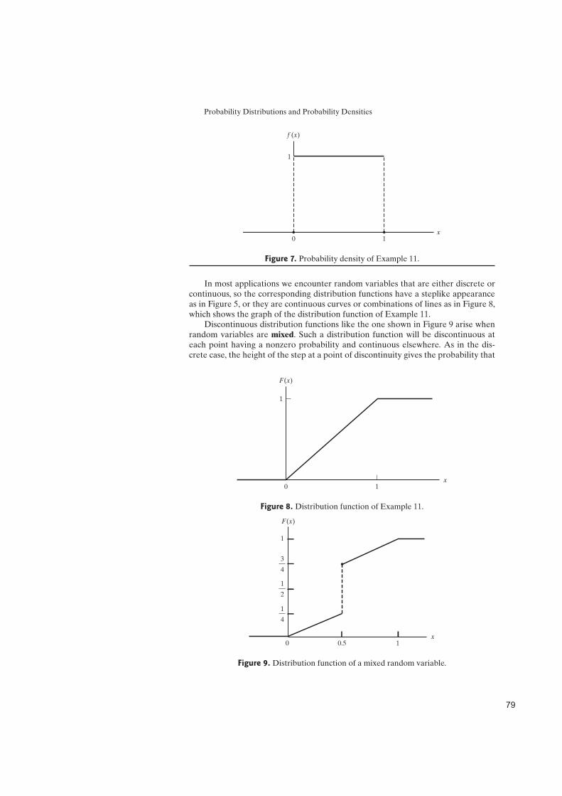
Probability Distributions and Probability Densities
0
f (x)
x1
1
Figure 7. Probability density of Example 11.
In most applications we encounter random variables that are either discrete orcontinuous, so the corresponding distribution functions have a steplike appearanceas in Figure 5, or they are continuous curves or combinations of lines as in Figure 8,which shows the graph of the distribution function of Example 11.
Discontinuous distribution functions like the one shown in Figure 9 arise whenrandom variables are mixed. Such a distribution function will be discontinuous ateach point having a nonzero probability and continuous elsewhere. As in the dis-crete case, the height of the step at a point of discontinuity gives the probability that
10x
F(x)
1
Figure 8. Distribution function of Example 11.
0
F(x)
x0.5 1
1
4
1
2
3
4
1
Figure 9. Distribution function of a mixed random variable.
%'

Probability Distributions and Probability Densities
the random variable will take on that particular value. With reference to Figure 9,P(X = 0.5) = 3
4 −14 =
12 , but otherwise the random variable is like a continuous
random variable.In this chapter we shall limit ourselves to random variables that are discrete or
continuous with the latter having distribution functions that are differentiable for allbut a finite set of values of the random variables.
Exercises
16. Find the distribution function of the random variableX of Exercise 17 and use it to reevaluate part (b).
17. The probability density of the continuous randomvariable X is given by
f (x) =
1
5for 2< x< 7
0 elsewhere
(a) Draw its graph and verify that the total area under thecurve (above the x-axis) is equal to 1.
(b) Find P(3<X < 5).
18. (a) Show that
f (x) = e−x for 0< x<q
represents a probability density function.
(b) Sketch a graph of this function and indicate the areaassociated with the probability that x> 1.
(c) Calculate the probability that x> 1.
19. (a) Show that
f (x) = 3x2 for 0< x< 1
represents a density function.
(b) Sketch a graph of this function, and indicate the areaassociated with the probability that 0.1< x< 0.5.
(c) Calculate the probability that 0.1< x< 0.5.
20. The probability density of the random variable Y isgiven by
f (y) =
1
8(y+ 1) for 2< y< 4
0 elsewhere
Find P(Y< 3.2) and P(2.9<Y< 3.2).
21. Find the distribution function of the random variableY of Exercise 20 and use it to determine the two proba-bilities asked for in that exercise.
22. The p.d.f. of the random variable X is given by
f (x) =
c√
xfor 0< x< 4
0 elsewhere
Find(a) the value of c;
(b) P(X < 14 ) and P(X > 1).
23. Find the distribution function of the random variableX of Exercise 22 and use it to determine the two proba-bilities asked for in part (b) of that exercise.
24. The probability density of the random variable Z isgiven by
f (z) =
{
kze−z2for z> 0
0 for z F 0
Find k and draw the graph of this probability density.
25. With reference to Exercise 24, find the distributionfunction of Z and draw its graph.
26. The density function of the random variable X isgiven by
g(x) =
{
6x(1− x) for 0< x< 1
0 elsewhere
Find P(X < 14 ) and P(X > 1
2 ).
27. With reference to Exercise 26, find the distributionfunction of X and use it to reevaluate the two probabili-ties asked for in that exercise.
28. Find the distribution function of the random variableX whose probability density is given by
f (x) =
x for 0< x< 1
2− x for 1 F x< 2
0 elsewhere
&(

Probability Distributions and Probability Densities
Also sketch the graphs of the probability density and dis-tribution functions.
29. Find the distribution function of the random variableX whose probability density is given by
f (x) =
1
3for 0< x< 1
1
3for 2< x< 4
0 elsewhere
Also sketch the graphs of the probability density and dis-tribution functions.
30. With reference to Exercise 28, find P(0.8<X < 1.2)using(a) the probability density;
(b) the distribution function.
31. Find the distribution function of the random variableX whose probability density is given by
f (x) =
x
2for 0< x F 1
1
2for 1< x F 2
3− x
2for 2< x< 3
0 elsewhere
Also sketch the graphs of these probability density anddistribution functions.
32. The distribution function of the random variable X isgiven by
F(x) =
0 for x<−1
x+ 1
2for −1 F x< 1
1 for x G 1
Find P(− 12 <X < 1
2 ) and P(2<X < 3).
33. With reference to Exercise 32, find the probabilitydensity of X and use it to recalculate the two proba-bilities.
34. The distribution function of the random variable Y isgiven by
F(y) =
1−9
y2for y> 3
0 elsewhere
Find P(Y F 5) and P(Y> 8).
35. With reference to Exercise 34, find the probabil-ity density of Y and use it to recalculate the twoprobabilities.
36. With reference to Exercise 34 and the result ofExercise 35, sketch the graphs of the distributionfunction and the probability density of Y, lettingf (3) = 0.
37. The distribution function of the random variable X isgiven by
F(x) =
{
1− (1+ x)e−x for x> 0
0 for x F 0
Find P(X F 2), P(1<X < 3), and P(X > 4).
38. With reference to Exercise 37, find the probabilitydensity of X.
39. With reference to Figure 9, find expressions for thevalues of the distribution function of the mixed randomvariable X for
(a) x F 0; (b) 0< x< 0.5;
(c) 0.5 F x< 1; (d) x G 1.
40. Use the results of Exercise 39 to find expressions forthe values of the probability density of the mixed randomvariable X for
(a) x< 0; (b) 0< x< 0.5;
(c) 0.5< x< 1; (d) x> 1.
P(X = 0.5) = 12 , and f (0) and f (1) are undefined.
41. The distribution function of the mixed random vari-able Z is given by
F(z) =
0 for z<−2
z+ 4
8for −2 F z< 2
1 for z G 2
Find P(Z = −2), P(Z = 2), P(−2<Z< 1), and P(0 F
Z F 2).
&)
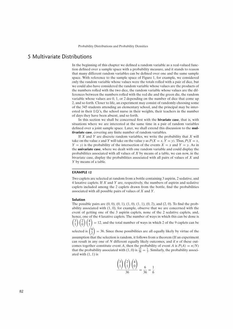
Probability Distributions and Probability Densities
5 Multivariate Distributions
In the beginning of this chapter we defined a random variable as a real-valued func-tion defined over a sample space with a probability measure, and it stands to reasonthat many different random variables can be defined over one and the same samplespace. With reference to the sample space of Figure 1, for example, we consideredonly the random variable whose values were the totals rolled with a pair of dice, butwe could also have considered the random variable whose values are the products ofthe numbers rolled with the two dice, the random variable whose values are the dif-ferences between the numbers rolled with the red die and the green die, the randomvariable whose values are 0, 1, or 2 depending on the number of dice that come up2, and so forth. Closer to life, an experiment may consist of randomly choosing someof the 345 students attending an elementary school, and the principal may be inter-ested in their I.Q.’s, the school nurse in their weights, their teachers in the numberof days they have been absent, and so forth.
In this section we shall be concerned first with the bivariate case, that is, withsituations where we are interested at the same time in a pair of random variablesdefined over a joint sample space. Later, we shall extend this discussion to the mul-
tivariate case, covering any finite number of random variables.If X and Y are discrete random variables, we write the probability that X will
take on the value x and Y will take on the value y as P(X = x, Y = y). Thus, P(X = x,Y = y) is the probability of the intersection of the events X = x and Y = y. As inthe univariate case, where we dealt with one random variable and could display theprobabilities associated with all values of X by means of a table, we can now, in thebivariate case, display the probabilities associated with all pairs of values of X andY by means of a table.
EXAMPLE 12
Two caplets are selected at random from a bottle containing 3 aspirin, 2 sedative, and4 laxative caplets. If X and Y are, respectively, the numbers of aspirin and sedativecaplets included among the 2 caplets drawn from the bottle, find the probabilitiesassociated with all possible pairs of values of X and Y.
Solution
The possible pairs are (0, 0), (0, 1), (1, 0), (1, 1), (0, 2), and (2, 0). To find the prob-ability associated with (1, 0), for example, observe that we are concerned with theevent of getting one of the 3 aspirin caplets, none of the 2 sedative caplets, and,hence, one of the 4 laxative caplets. The number of ways in which this can be done is(
31
)(
20
)(
41
)
= 12, and the total number of ways in which 2 of the 9 caplets can be
selected is
(
92
)
= 36. Since those possibilities are all equally likely by virtue of the
assumption that the selection is random, it follows from a theorem (If an experimentcan result in any one of N different equally likely outcomes, and if n of these out-comes together constitute event A, then the probability of event A is P(A) = n/N)
that the probability associated with (1, 0) is 1236 =
13 . Similarly, the probability associ-
ated with (1, 1) is(
31
)(
21
)(
40
)
36=
6
36=
1
6
&!
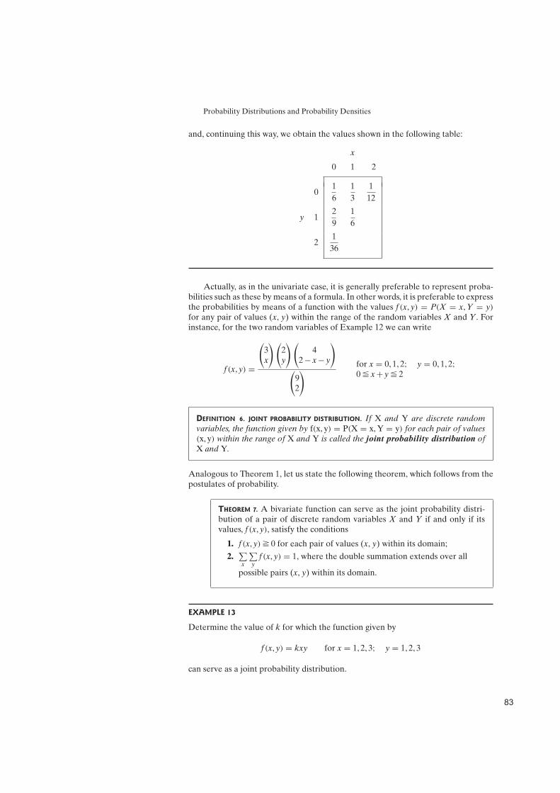
Probability Distributions and Probability Densities
and, continuing this way, we obtain the values shown in the following table:
x
0 1 2
01
6
1
3
1
12
y 12
9
1
6
21
36
Actually, as in the univariate case, it is generally preferable to represent proba-bilities such as these by means of a formula. In other words, it is preferable to expressthe probabilities by means of a function with the values f (x, y) = P(X = x, Y = y)
for any pair of values (x, y) within the range of the random variables X and Y. Forinstance, for the two random variables of Example 12 we can write
f (x, y) =
(
3x
)(
2y
)(
42− x− y
)
(
92
)
for x = 0, 1, 2; y = 0, 1, 2;0 F x+ y F 2
DEFINITION 6. JOINT PROBABILITY DISTRIBUTION. If X and Y are discrete random
variables, the function given by f(x, y) = P(X = x, Y = y) for each pair of values
(x, y) within the range of X and Y is called the joint probability distribution of
X and Y.
Analogous to Theorem 1, let us state the following theorem, which follows from thepostulates of probability.
THEOREM 7. A bivariate function can serve as the joint probability distri-bution of a pair of discrete random variables X and Y if and only if itsvalues, f (x, y), satisfy the conditions
1. f (x, y) G 0 for each pair of values (x, y) within its domain;
2.∑
x
∑
yf (x, y) = 1, where the double summation extends over all
possible pairs (x, y) within its domain.
EXAMPLE 13
Determine the value of k for which the function given by
f (x, y) = kxy for x = 1, 2, 3; y = 1, 2, 3
can serve as a joint probability distribution.
&"

Probability Distributions and Probability Densities
Solution
Substituting the various values of x and y, we get f (1, 1) = k, f (1, 2) = 2k, f (1, 3) =3k, f (2, 1) = 2k, f (2, 2) = 4k, f (2, 3) = 6k, f (3, 1) = 3k, f (3, 2) = 6k, and f (3, 3) = 9k.To satisfy the first condition of Theorem 7, the constant k must be nonnegative, andto satisfy the second condition,
k+ 2k+ 3k+ 2k+ 4k+ 6k+ 3k+ 6k+ 9k = 1
so that 36k = 1 and k = 136 .
As in the univariate case, there are many problems in which it is of interest toknow the probability that the values of two random variables are less than or equalto some real numbers x and y.
DEFINITION 7. JOINT DISTRIBUTION FUNCTION. If X and Y are discrete random vari-
ables, the function given by
F(x, y) = P(X ≤ x, Y ≤ y) =∑
s≤x
∑
t≤y
f (s, t) for −q< x<q
−q< y<q
where f(s, t) is the value of the joint probability distribution of X and Y at (s, t), is
called the joint distribution function, or the joint cumulative distribution of Xand Y.
In Exercise 48 the reader will be asked to prove properties of joint distribution func-tions that are analogous to those of Theorem 2.
EXAMPLE 14
With reference to Example 12, find F(1, 1).
SolutionF(1, 1) = P(X F 1, Y F 1)
= f (0, 0)+ f (0, 1)+ f (1, 0)+ f (1, 1)
=1
6+
2
9+
1
3+
1
6
=8
9
As in the univariate case, the joint distribution function of two random variablesis defined for all real numbers. For instance, for Example 12 we also get F(−2, 1) =P(X F −2, Y F 1) = 0 and F(3.7, 4.5) = P(X F 3.7, Y F 4.5) = 1.
Let us now extend the various concepts introduced in this section to the contin-uous case.
&#

Probability Distributions and Probability Densities
DEFINITION 8. JOINT PROBABILITY DENSITY FUNCTION. A bivariate function with
values f(x, y) defined over the xy-plane is called a joint probability densityfunction of the continuous random variables X and Y if and only if
P(X, Y) ∈ A =∫∫
A
f (x, y)dxdy
for any region A in the xy-plane.
Analogous to Theorem 5, it follows from the postulates of probability that
THEOREM 8. A bivariate function can serve as a joint probability densityfunction of a pair of continuous random variables X and Y if its values,f (x, y), satisfy the conditions
1. f (x, y) G 0 for −q< x<q, −q< y<q;
2.
∫
q
−q
∫
q
−qf (x, y)dx dy = 1.
EXAMPLE 15
Given the joint probability density function
f (x, y) =
3
5x(y+ x) for 0< x< 1, 0< y< 2
0 elsewhere
of two random variables X and Y, find P[(X, Y) ∈ A], where A is the region {(x, y)|0<x< 1
2 , 1< y< 2}.
Solution
P[(X, Y) ∈ A] = P
(
0<X <1
2, 1<Y< 2
)
=∫ 2
1
∫ 12
0
3
5x(y+ x)dx dy
=∫ 2
1
3x2y
10+
3x3
15
∣
∣
∣
∣
∣
x= 12
dy
=∫ 2
1
(
3y
40+
1
40
)
dy =3y2
80+
y
40
∣
∣
∣
∣
2
1
=11
80
Analogous to Definition 7, we have the following definition of the joint distribu-tion function of two continuous random variables.
&$

Probability Distributions and Probability Densities
DEFINITION 9. JOINT DISTRIBUTION FUNCTION. If X and Y are continuous random
variables, the function given by
F(x, y) = P(X ≤ x, Y ≤ y) =∫ y
−q
∫ x
−qf (s, t)ds dt for −q< x<q,
−q< y<q
where f(s, t) is the joint probability density of X and Y at (s, t), is called the jointdistribution function of X and Y.
Note that the properties of joint distribution functions, which the reader will beasked to prove in Exercise 48 for the discrete case, hold also for the continuous case.
As in Section 4, we shall limit our discussion here to random variables whosejoint distribution function is continuous everywhere and partially differentiable withrespect to each variable for all but a finite set of values of the two random variables.
Analogous to the relationship f (x) =dF(x)
dxof Theorem 6, partial differentia-
tion in Definition 9 leads to
f (x, y) =
2
xyF(x, y)
wherever these partial derivatives exist. As in Section 4, the joint distribution func-tion of two continuous random variables determines their joint density (short forjoint probability density function) at all points (x, y) where the joint density is con-tinuous. Also as in Section 4, we generally let the values of joint probability densitiesequal zero wherever they are not defined by the above relationship.
EXAMPLE 16
If the joint probability density of X and Y is given by
f (x, y) =
{
x+ y for 0< x< 1, 0< y< 1
0 elsewhere
find the joint distribution function of these two random variables.
Solution
If either x< 0 or y< 0, it follows immediately that F(x, y) = 0. For 0< x< 1 and0< y< 1 (Region I of Figure 10), we get
F(x, y) =∫ y
0
∫ x
0(s+ t)ds dt =
1
2xy(x+ y)
for x> 1 and 0< y< 1 (Region II of Figure 10), we get
F(x, y) =∫ y
0
∫ 1
0(s+ t)ds dt =
1
2y(y+ 1)
&

Probability Distributions and Probability Densities
Figure 10. Diagram for Example 16.
for 0< x< 1 and y> 1 (Region III of Figure 10), we get
F(x, y) =∫ 1
0
∫ x
0(s+ t)ds dt =
1
2x(x+ 1)
and for x> 1 and y> 1 (Region IV of Figure 10), we get
F(x, y) =∫ 1
0
∫ 1
0(s+ t)ds dt = 1
Since the joint distribution function is everywhere continuous, the boundariesbetween any two of these regions can be included in either one, and we can write
F(x, y) =
0 for x F 0 or y F 0
1
2xy(x+ y) for 0< x< 1, 0< y< 1
1
2y(y+ 1) for x G 1, 0< y< 1
1
2x(x+ 1) for 0< x< 1, y G 1
1 for x G 1, y G 1
EXAMPLE 17
Find the joint probability density of the two random variables X and Y whose jointdistribution function is given by
F(x, y) =
{
(1− e−x)(1− e−y) for x> 0 and y> 0
0 elsewhere
Also use the joint probability density to determine P(1<X < 3, 1<Y < 2).
&%

Probability Distributions and Probability Densities
Solution
Since partial differentiation yields
2
xyF(x, y) = e−(x+y)
for x> 0 and y> 0 and 0 elsewhere, we find that the joint probability density of X
and Y is given by
f (x, y) =
{
e−(x+y) for x> 0 and y> 0
0 elsewhere
Thus, integration yields
∫ 2
1
∫ 3
1e−(x+y) dx dy = (e−1− e−3)(e−1− e−2)
= e−2− e−3− e−4+ e−5
= 0.074
for P(1<X < 3, 1<Y < 2).
For two random variables, the joint probability is, geometrically speaking, a sur-face, and the probability that we calculated in the preceding example is given by thevolume under this surface, as shown in Figure 11.
All the definitions of this section can be generalized to the multivariate case,where there are n random variables. Corresponding to Definition 6, the values ofthe joint probability distribution of n discrete random variables X1, X2, . . ., and Xn
are given by
f (x1, x2, . . . , xn) = P(X1 = x1, X2 = x2, . . . , Xn = xn)
f (x, y)
x
y
f (x, y) e (x y)
1
1 2 3
2
3
Figure 11. Diagram for Example 17.
&&

Probability Distributions and Probability Densities
for each n-tuple (x1, x2, . . . , xn) within the range of the random variables; and corre-sponding to Definition 7, the values of their joint distribution function are given by
F(x1, x2, . . . , xn) = P(X1 F x1, X2 F x2, . . . , Xn F xn)
for −q< x1<q,−q< x2<q, . . . ,−q< xn<q.
EXAMPLE 18
If the joint probability distribution of three discrete random variables X, Y, and Z
is given by
f (x, y, z) =(x+ y)z
63for x = 1, 2; y = 1, 2, 3; z = 1, 2
find P(X = 2, Y+Z F 3).
SolutionP(X = 2, Y+Z F 3) = f (2, 1, 1)+ f (2, 1, 2)+ f (2, 2, 1)
=3
63+
6
63+
4
63
=13
63
In the continuous case, probabilities are again obtained by integrating the jointprobability density, and the joint distribution function is given by
F(x1, x2, . . . , xn) =∫ xn
−q. . .
∫ x2
−q
∫ x1
−qf (t1, t2, . . . , tn)dt1 dt2 . . . dtn
for −q< x1<q,−q< x2<q, . . . ,−q< xn<q, analogous to Definition 9. Also,partial differentiation yields
f (x1, x2, . . . , xn) =
n
x1x2 · · · xnF(x1, x2, . . . , xn)
wherever these partial derivatives exist.
EXAMPLE 19
If the trivariate probability density of X1, X2, and X3 is given by
f (x1, x2, x3) =
{
(x1+ x2)e−x3 for 0< x1< 1, 0< x2< 1, x3> 0
0 elsewhere
find P[(X1, X2, X3) ∈ A], where A is the region
{
(x1, x2, x3)|0< x1<1
2,
1
2< x2< 1, x3< 1
}
&'

Probability Distributions and Probability Densities
Solution
P[(X1, X2, X3) ∈ A] = P
(
0<X1<1
2,
1
2<X2< 1, X3< 1
)
=∫ 1
0
∫ 1
12
∫ 12
0(x1+ x2)e
−x3 dx1 dx2 dx3
=∫ 1
0
∫ 1
12
(
1
8+
x2
2
)
e−x3 dx2 dx3
=∫ 1
0
1
4e−x3 dx3
=1
4(1− e−1) = 0.158
Exercises
42. If the values of the joint probability distribution of Xand Y are as shown in the table
x0 1 2
01
12
1
6
1
24
11
4
1
4
1
40
y2
1
8
1
20
31
120
find
(a) P(X = 1, Y = 2); (b) P(X = 0, 1 F Y< 3);
(c) P(X +Y F 1); (d) P(X >Y).
43. With reference to Exercise 42, find the following val-ues of the joint distribution function of the two ran-dom variables:
(a) F(1.2, 0.9); (b) F(−3, 1.5);
(c) F(2, 0); (d) F(4, 2.7).
44. If the joint probability distribution of X and Y isgiven by
f (x, y) = c(x2+ y2) for x = −1, 0, 1, 3; y = −1, 2, 3
find the value of c.
45. With reference to Exercise 44 and the value obtai-ned for c, find(a) P(X F 1, Y> 2);
(b) P(X = 0, Y F 2);
(c) P(X +Y> 2).
46. Show that there is no value of k for which
f (x, y) = ky(2y− x) for x = 0, 3; y = 0, 1, 2
can serve as the joint probability distribution of two ran-dom variables.
47. If the joint probability distribution of X and Y isgiven by
f (x, y) =1
30(x+ y) for x = 0, 1, 2, 3; y = 0, 1, 2
construct a table showing the values of the joint distribu-tion function of the two random variables at the 12 points(0, 0), (0, 1), . . . , (3, 2).
48. If F(x, y) is the value of the joint distribution func-tion of two discrete random variables X and Y at (x, y),show that(a) F(−q,−q) = 0;
(b) F(q,q) = 1;
(c) if a<b and c<d, then F(a, c) F F(b, d).
49. Determine k so that
f (x, y) ={
kx(x− y) for 0< x< 1,−x< y< x
0 elsewhere
can serve as a joint probability density.
50. If the joint probability density of X and Y is given by
f (x, y) ={
24xy for 0< x< 1, 0< y< 1, x+ y< 1
0 elsewhere
find P(X +Y< 12 ).
'(

Probability Distributions and Probability Densities
51. If the joint probability density of X and Y is given by
f (x, y) =
{
2 for x> 0, y> 0, x+ y< 1
0 elsewhere
find(a) P(X F
12 , Y F
12 );
(b) P(X +Y> 23 );
(c) P(X > 2Y).
52. With reference to Exercise 51, find an expression forthe values of the joint distribution function of X and Ywhen x> 0, y> 0, and x+ y< 1, and use it to verify theresult of part (a).
53. If the joint probability density of X and Y is given by
f (x, y) =
1
yfor 0< x< y, 0< y< 1
0 elsewhere
find the probability that the sum of the values of X and Y
will exceed 12 .
54. Find the joint probability density of the two randomvariables X and Y whose joint distribution function isgiven by
F(x, y) =
{
(1− e−x2)(1− e−y2
) for x> 0, y> 0
0 elsewhere
55. Use the joint probability density obtained in Exer-cise 54 to find P(1<X F 2, 1<Y F 2).
56. Find the joint probability density of the two randomvariables X and Y whose joint distribution function isgiven by
F(x, y) =
{
1− e−x− e−y+ e−x−y for x> 0, y> 0
0 elsewhere
57. Use the joint probability density obtained in Exer-cise 56 to find P(X +Y> 3).
58. If F(x, y) is the value of the joint distribution func-tion of the two continuous random variables X and Y at(x, y), express P(a<X F b, c<Y F d) in terms of F(a, c),F(a, d), F(b, c), and F(b, d). Observe that the result holdsalso for discrete random variables.
59. Use the formula obtained in Exercise 58 to verify theresult, 0.074, of Example 17.
60. Use the formula obtained in Exercise 58 to verify theresult of Exercise 55.
61. Use the formula obtained in Exercise 58 to verify theresult of Exercise 57.
62. Find k if the joint probability distribution of X, Y, andZ is given by
f (x, y, z) = kxyz
for x = 1, 2; y = 1, 2, 3; z = 1, 2.
63. With reference to Exercise 62, find(a) P(X = 1, Y F 2, Z = 1);
(b) P(X = 2, Y+Z = 4).
64. With reference to Exercise 62, find the following val-ues of the joint distribution function of the three ran-dom variables:(a) F(2, 1, 2);
(b) F(1, 0, 1);
(c) F(4, 4, 4).
65. Find k if the joint probability density of X, Y, and Zis given by
f (x, y, z) =
kxy(1− z) for 0< x< 1, 0< y< 1,
0< z< 1, x+ y+ z< 1
0 elsewhere
66. With reference to Exercise 65, find P(X +Y< 12 ).
67. Use the result of Example 16 to verify that the jointdistribution function of the random variables X1, X2, andX3 of Example 19 is given by
F(x1, x2, x3) =
0 for x1 F 0, x2 F 0, or x3 F 0
1
2x1x2(x1 + x2)(1− e−x3 ) for 0< x1 < 1, 0< x2 < 1, x3 > 0
1
2x2(x2 + 1)(1− e−x3 ) for x1 G 1, 0< x2 < 1, x3 > 0
1
2x1(x1 + 1)(1− e−x3 ) for 0< x1 < 1, x2 G 1, x3 > 0
1− e−x3 for x1 G 1, x2 G 1, x3 > 0
68. If the joint probability density of X, Y, and Z isgiven by
f (x, y, z) =
1
3(2x+ 3y+ z) for 0< x< 1, 0< y< 1,
0< z< 1
0 elsewhere
find(a) P(X = 1
2 , Y = 12 , Z = 1
2 );
(b) P(X < 12 , Y< 1
2 , Z< 12 ).
')

Probability Distributions and Probability Densities
6 Marginal Distributions
To introduce the concept of a marginal distribution, let us consider the followingexample.
EXAMPLE 20
In Example 12 we derived the joint probability distribution of two random variablesX and Y, the number of aspirin caplets and the number of sedative caplets includedamong two caplets drawn at random from a bottle containing three aspirin, two seda-tive, and four laxative caplets. Find the probability distribution of X alone and thatof Y alone.
Solution
The results of Example 12 are shown in the following table, together with the marginaltotals, that is, the totals of the respective rows and columns:
x
0 1 2
01
6
1
3
1
12
7
12
y 12
9
1
6
7
18
21
36
1
36
5
12
1
2
1
12
The column totals are the probabilities that X will take on the values 0, 1, and 2. Inother words, they are the values
g(x) =2∑
y=0
f (x, y) for x = 0, 1, 2
of the probability distribution of X. By the same token, the row totals are the values
h(y) =2∑
x=0
f (x, y) for y = 0, 1, 2
of the probability distribution of Y.
We are thus led to the following definition.
DEFINITION 10. MARGINAL DISTRIBUTION. If X and Y are discrete random variables
and f(x, y) is the value of their joint probability distribution at (x, y), the function
given by
g(x) =∑
y
f (x, y)
'!
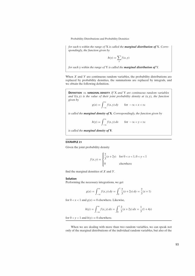
Probability Distributions and Probability Densities
for each x within the range of X is called the marginal distribution of X. Corre-
spondingly, the function given by
h(y) =∑
x
f (x, y)
for each y within the range of Y is called the marginal distribution of Y.
When X and Y are continuous random variables, the probability distributions arereplaced by probability densities, the summations are replaced by integrals, andwe obtain the following definition.
DEFINITION 11. MARGINAL DENSITY. If X and Y are continuous random variables
and f(x, y) is the value of their joint probability density at (x, y), the function
given by
g(x) =∫
q
−qf (x, y)dy for −q< x<q
is called the marginal density of X. Correspondingly, the function given by
h(y) =∫
q
−qf (x, y)dx for −q< y<q
is called the marginal density of Y.
EXAMPLE 21
Given the joint probability density
f (x, y) =
2
3(x+ 2y) for 0< x< 1, 0< y< 1
0 elsewhere
find the marginal densities of X and Y.
Solution
Performing the necessary integrations, we get
g(x) =∫
q
−qf (x, y)dy =
∫ 1
0
2
3(x+ 2y)dy =
2
3(x+ 1)
for 0< x< 1 and g(x) = 0 elsewhere. Likewise,
h(y) =∫
q
−qf (x, y)dx =
∫ 1
0
2
3(x+ 2y)dx =
1
3(1+ 4y)
for 0< y< 1 and h(y) = 0 elsewhere.
When we are dealing with more than two random variables, we can speak notonly of the marginal distributions of the individual random variables, but also of the
'"
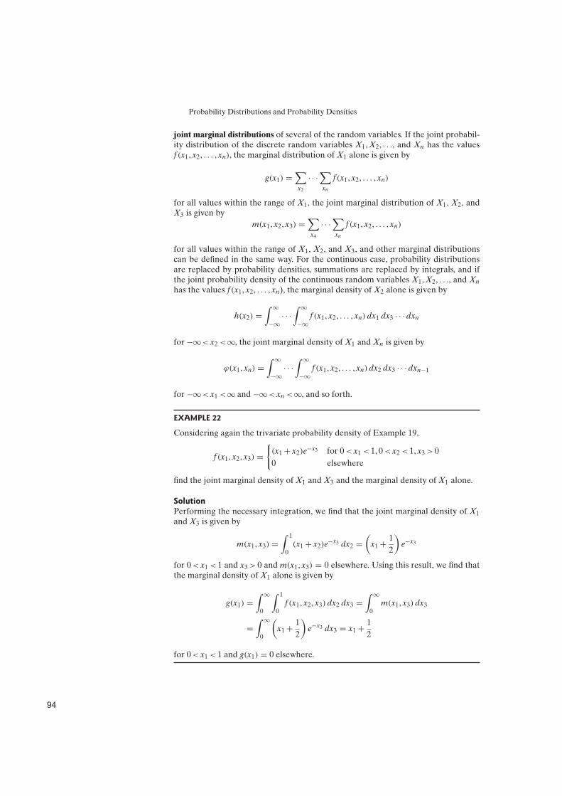
Probability Distributions and Probability Densities
joint marginal distributions of several of the random variables. If the joint probabil-ity distribution of the discrete random variables X1, X2, . . ., and Xn has the valuesf (x1, x2, . . . , xn), the marginal distribution of X1 alone is given by
g(x1) =∑
x2
· · ·∑
xn
f (x1, x2, . . . , xn)
for all values within the range of X1, the joint marginal distribution of X1, X2, andX3 is given by
m(x1, x2, x3) =∑
x4
· · ·∑
xn
f (x1, x2, . . . , xn)
for all values within the range of X1, X2, and X3, and other marginal distributionscan be defined in the same way. For the continuous case, probability distributionsare replaced by probability densities, summations are replaced by integrals, and ifthe joint probability density of the continuous random variables X1, X2, . . ., and Xn
has the values f (x1, x2, . . . , xn), the marginal density of X2 alone is given by
h(x2) =∫
q
−q· · ·∫
q
−qf (x1, x2, . . . , xn)dx1 dx3 · · ·dxn
for −q< x2<q, the joint marginal density of X1 and Xn is given by
ϕ(x1, xn) =∫
q
−q· · ·∫
q
−qf (x1, x2, . . . , xn)dx2 dx3 · · · dxn−1
for −q< x1<q and −q< xn<q, and so forth.
EXAMPLE 22
Considering again the trivariate probability density of Example 19,
f (x1, x2, x3) =
{
(x1+ x2)e−x3 for 0< x1< 1, 0< x2< 1, x3> 0
0 elsewhere
find the joint marginal density of X1 and X3 and the marginal density of X1 alone.
Solution
Performing the necessary integration, we find that the joint marginal density of X1
and X3 is given by
m(x1, x3) =∫ 1
0(x1+ x2)e
−x3 dx2 =(
x1+1
2
)
e−x3
for 0< x1< 1 and x3> 0 and m(x1, x3) = 0 elsewhere. Using this result, we find thatthe marginal density of X1 alone is given by
g(x1) =∫
q
0
∫ 1
0f (x1, x2, x3)dx2 dx3 =
∫
q
0m(x1, x3)dx3
=∫
q
0
(
x1+1
2
)
e−x3 dx3 = x1+1
2
for 0< x1< 1 and g(x1) = 0 elsewhere.
'#

Probability Distributions and Probability Densities
Corresponding to the various marginal and joint marginal distributions and den-sities we have introduced in this section, we can also define marginal and joint
marginal distribution functions. Some problems relating to such distribution func-tions will be left to the reader in Exercises 72, 79, and 80.
7 Conditional Distributions
In the conditional probability of event A, given event B, as
P(A|B) =P(A∩B)
P(B)
provided P(B)Z 0. Suppose now that A and B are the events X = x and Y = y sothat we can write
P(X = x|Y = y) =P(X = x, Y = y)
P(Y = y)
=f (x, y)
h(y)
provided P(Y = y) = h(y)Z 0, where f (x, y) is the value of the joint probabilitydistribution of X and Y at (x, y), and h(y) is the value of the marginal distribution ofY at y. Denoting the conditional probability by f (x|y) to indicate that x is a variableand y is fixed, let us now make the following definition.
DEFINITION 12. CONDITIONAL DISTRIBUTION. If f(x, y) is the value of the joint prob-
ability distribution of the discrete random variables X and Y at (x, y) and h(y) is
the value of the marginal distribution of Y at y, the function given by
f (x|y) =f (x, y)
h(y)h(y)Z 0
for each x within the range of X is called the conditional distribution of X givenY = y. Correspondingly, if g(x) is the value of the marginal distribution of X at x,
the function given by
w(y|x) =f (x, y)
g(x)g(x)Z 0
for each y within the range of Y is called the conditional distribution of Y givenX = x.
EXAMPLE 23
With reference to Examples 12 and 20, find the conditional distribution of X
given Y = 1.
Solution
Substituting the appropriate values from the table in Example 20, we get
f (0|1) =
2
97
18
=4
7
'$

Probability Distributions and Probability Densities
f (1|1) =
1
67
18
=3
7
f (2|1) =0
7
18
= 0
When X and Y are continuous random variables, the probability distributionsare replaced by probability densities, and we obtain the following definition.
DEFINITION 13. CONDITIONAL DENSITY. If f(x, y) is the value of the joint density of
the continuous random variables X and Y at (x, y) and h(y) is the value of the
marginal distribution of Y at y, the function given by
f (x|y) =f (x, y)
h(y)h(y)Z 0
for−q< x<q, is called the conditional density of X given Y = y. Correspond-
ingly, if g(x) is the value of the marginal density of X at x, the function
given by
w(y|x) =f (x, y)
g(x)g(x)Z 0
for −q< y<q, is called the conditional density of Y given X = x.
EXAMPLE 24
With reference to Example 21, find the conditional density of X given Y = y, anduse it to evaluate P(X F
12 |Y = 1
2 ).
Solution
Using the results obtained on the previous page, we have
f (x|y) =f (x, y)
h(y)=
2
3(x+ 2y)
1
3(1+ 4y)
=2x+ 4y
1+ 4y
for 0< x< 1 and f (x|y) = 0 elsewhere. Now,
f
(
x
∣
∣
∣
∣
1
2
)
=2x+ 4 ·
1
2
1+ 4 ·1
2
=2x+ 2
3
'

Probability Distributions and Probability Densities
and we can write
P
(
X F1
2
∣
∣
∣
∣
Y =1
2
)
=∫ 1
2
0
2x+ 2
3dx =
5
12
It is of interest to note that in Figure 12 this probability is given by the ratio of thearea of trapezoid ABCD to the area of trapezoid AEFD.
Figure 12. Diagram for Example 24.
EXAMPLE 25
Given the joint probability density
f (x, y) =
{
4xy for 0< x< 1, 0< y< 1
0 elsewhere
find the marginal densities of X and Y and the conditional density of X given Y = y.
Solution
Performing the necessary integrations, we get
g(x) =∫
q
−qf (x, y)dy =
∫ 1
04xy dy
= 2xy2
∣
∣
∣
∣
∣
y=1
y=0
= 2x
for 0< x< 1, and g(x) = 0 elsewhere; also
h(y) =∫
q
−qf (x, y)dx =
∫ 1
04xy dx
= 2x2y
∣
∣
∣
∣
∣
x=1
x=0
= 2y
'%

Probability Distributions and Probability Densities
for 0< y< 1, and h(y) = 0 elsewhere. Then, substituting into the formula for a con-ditional density, we get
f (x|y) =f (x, y)
h(y)=
4xy
2y= 2x
for 0< x< 1, and f (x|y) = 0 elsewhere.
When we are dealing with more than two random variables, whether continuousor discrete, we can consider various different kinds of conditional distributions ordensities. For instance, if f (x1, x2, x3, x4) is the value of the joint distribution of thediscrete random variables X1, X2, X3, and X4 at (x1, x2, x3, x4), we can write
p(x3|x1, x2, x4) =f (x1, x2, x3, x4)
g(x1, x2, x4)g(x1, x2, x4)Z 0
for the value of the conditional distribution of X3 at x3 given X1 = x1, X2 = x2, andX4 = x4, where g(x1, x2, x4) is the value of the joint marginal distribution of X1, X2,and X4 at (x1, x2, x4). We can also write
q(x2, x4|x1, x3) =f (x1, x2, x3, x4)
m(x1, x3)m(x1, x3)Z 0
for the value of the joint conditional distribution of X2 and X4 at (x2, x4) givenX1 = x1 and X3 = x3, or
r(x2, x3, x4|x1) =f (x1, x2, x3, x4)
b(x1)b(x1)Z 0
for the value of the joint conditional distribution of X2, X3, and X4 at (x2, x3, x4)
given X1 = x1.When we are dealing with two or more random variables, questions of indepen-
dence are usually of great importance. In Example 25 we see that f (x|y) = 2x doesnot depend on the given value Y = y, but this is clearly not the case in Example 24,
where f (x|y) =2x+ 4y
1+ 4y. Whenever the values of the conditional distribution of X
given Y = y do not depend on y, it follows that f (x|y) = g(x), and hence the formulasof Definitions 12 and 13 yield
f (x, y) = f (x|y) ·h(y) = g(x) ·h(y)
That is, the values of the joint distribution are given by the products of the corre-sponding values of the two marginal distributions. Generalizing from this observa-tion, let us now make the following definition.
DEFINITION 14. INDEPENDENCE OF DISCRETE RANDOM VARIABLES. If f(x1, x2, . . . , xn) is
the value of the joint probability distribution of the discrete random variables
X1, X2, . . . , Xn at (x1, x2, . . . , xn) and fi(xi) is the value of the marginal distribution
of Xi at xi for i = 1, 2, . . . , n, then the n random variables are independent if and
only if
f (x1, x2, . . . , xn) = f1(x1) · f2(x2) · . . . · fn(xn)
for all (x1, x2, . . . , xn) within their range.
To give a corresponding definition for continuous random variables, we simplysubstitute the word “density” for the word “distribution.”
With this definition of independence, it can easily be verified that the three ran-dom variables of Example 22 are not independent, but that the two random variables
'&

Probability Distributions and Probability Densities
X1 and X3 and also the two random variables X2 and X3 are pairwise independent
(see Exercise 81).The following examples serve to illustrate the use of Definition 14 in finding
probabilities relating to several independent random variables.
EXAMPLE 26
Considering n independent flips of a balanced coin, let Xi be the number of heads(0 or 1) obtained in the ith flip for i = 1, 2, . . . , n. Find the joint probability distribu-tion of these n random variables.
Solution
Since each of the random variables Xi, for i = 1, 2, . . . , n, has the probability distri-bution
fi(xi) =1
2for xi = 0, 1
and the n random variables are independent, their joint probability distribution isgiven by
f (x1, x2, . . . , xn) = f1(x1) · f2(x2) · . . . · fn(xn)
=1
2·
1
2· . . . ·
1
2=(
1
2
)n
where xi = 0 or 1 for i = 1, 2, . . . , n.
EXAMPLE 27
Given the independent random variables X1, X2, and X3 with the probabilitydensities
f1(x1) =
{
e−x1 for x1> 0
0 elsewhere
f2(x2) =
{
2e−2x2 for x2> 0
0 elsewhere
f3(x3) ={
3e−3x3 for x3> 0
0 elsewhere
find their joint probability density, and use it to evaluate the probability P(X1+X2 F 1, X3> 1).
Solution
According to Definition 14, the values of the joint probability density aregiven by
f (x1, x2, x3) = f1(x1) · f2(x2) · f3(x3)
= e−x1 · 2e−2x2 · 3e−3x3
= 6e−x1−2x2−3x3
''
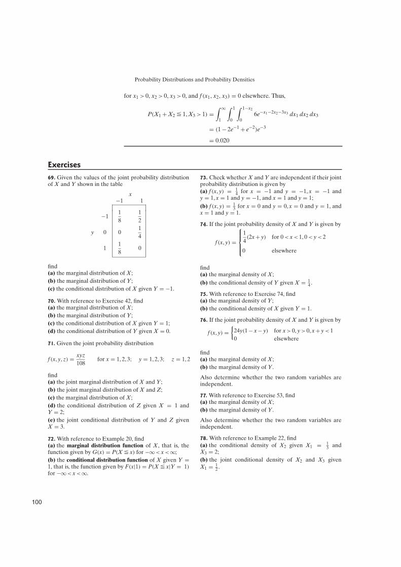
Probability Distributions and Probability Densities
for x1> 0, x2> 0, x3> 0, and f (x1, x2, x3) = 0 elsewhere. Thus,
P(X1+X2 F 1, X3> 1) =∫
q
1
∫ 1
0
∫ 1−x2
06e−x1−2x2−3x3 dx1 dx2 dx3
= (1− 2e−1+ e−2)e−3
= 0.020
Exercises
69. Given the values of the joint probability distributionof X and Y shown in the table
x−1 1
−11
8
1
2
y 0 01
4
11
80
find(a) the marginal distribution of X;
(b) the marginal distribution of Y;
(c) the conditional distribution of X given Y = −1.
70. With reference to Exercise 42, find(a) the marginal distribution of X;
(b) the marginal distribution of Y;
(c) the conditional distribution of X given Y = 1;
(d) the conditional distribution of Y given X = 0.
71. Given the joint probability distribution
f (x, y, z) =xyz
108for x = 1, 2, 3; y = 1, 2, 3; z = 1, 2
find(a) the joint marginal distribution of X and Y;
(b) the joint marginal distribution of X and Z;
(c) the marginal distribution of X;
(d) the conditional distribution of Z given X = 1 andY = 2;
(e) the joint conditional distribution of Y and Z givenX = 3.
72. With reference to Example 20, find(a) the marginal distribution function of X, that is, thefunction given by G(x) = P(X F x) for −q< x<q;
(b) the conditional distribution function of X given Y =1, that is, the function given by F(x|1) = P(X F x|Y = 1)for −q< x<q.
73. Check whether X and Y are independent if their jointprobability distribution is given by(a) f (x, y) = 1
4 for x = −1 and y = −1, x = −1 andy = 1, x = 1 and y = −1, and x = 1 and y = 1;
(b) f (x, y) = 13 for x = 0 and y = 0, x = 0 and y = 1, and
x = 1 and y = 1.
74. If the joint probability density of X and Y is given by
f (x, y) =
1
4(2x+ y) for 0< x< 1, 0< y< 2
0 elsewhere
find(a) the marginal density of X;
(b) the conditional density of Y given X = 14 .
75. With reference to Exercise 74, find(a) the marginal density of Y;
(b) the conditional density of X given Y = 1.
76. If the joint probability density of X and Y is given by
f (x, y) ={
24y(1− x− y) for x> 0, y> 0, x+ y< 1
0 elsewhere
find(a) the marginal density of X;
(b) the marginal density of Y.
Also determine whether the two random variables areindependent.
77. With reference to Exercise 53, find(a) the marginal density of X;
(b) the marginal density of Y.
Also determine whether the two random variables areindependent.
78. With reference to Example 22, find(a) the conditional density of X2 given X1 = 1
3 andX3 = 2;
(b) the joint conditional density of X2 and X3 givenX1 = 1
2 .
)((

Probability Distributions and Probability Densities
79. If F(x, y) is the value of the joint distribution functionof X and Y at (x, y), show that the marginal distributionfunction of X is given by
G(x) = F(x,q) for −q< x<q
Use this result to find the marginal distribution functionof X for the random variables of Exercise 54.
80. If F(x1, x2, x3) is the value of the joint distributionfunction of X1, X2, and X3 at (x1, x2, x3), show that thejoint marginal distribution function of X1 and X3 isgiven by
M(x1, x3) = F(x1,q, x3) for −q< x1<q,−q< x3<q
and that the marginal distribution function of X1 isgiven by
G(x1) = F(x1,q,q) for −q< x1<q
With reference to Example 19, use these results to find
(a) the joint marginal distribution function of X1 and X3;
(b) the marginal distribution function of X1.
81. With reference to Example 22, verify that the threerandom variables X1, X2, and X3 are not independent,but that the two random variables X1 and X3 andalso the two random variables X2 and X3 are pairwiseindependent.
82. If the independent random variables X and Y havethe marginal densities
f (x) =
1
2for 0< x< 2
0 elsewhere
π(y) =
1
3for 0< y< 3
0 elsewhere
find(a) the joint probability density of X and Y;
(b) the value of P(X2+Y2> 1).
8 The Theory in Practice
This chapter has been about how probabilities can group themselves into probabilitydistributions, and how, in the case of continuous random variables, these distribu-tions become probability density functions. In practice, however, all data appear tobe discrete. (Even if data arise from continuous random variables, the limitationsof measuring instruments and roundoff produce discrete values.) In this section, weshall introduce some applications of the ideas of probability distributions and den-sities to the exploration of raw data, an important element of what is called data
analysis.When confronted with raw data, often consisting of a long list of measurements,
it is difficult to understand what the data are informing us about the process, product,or service which gave rise to them. The following data, giving the response times of30 integrated circuits (in picoseconds), illustrate this point:
Integrated Circuit Response Times (ps)
4.6 4.0 3.7 4.1 4.1 5.6 4.5 6.0 6.0 3.4
3.4 4.6 3.7 4.2 4.6 4.7 4.1 3.7 3.4 3.3
3.7 4.1 4.5 4.6 4.4 4.8 4.3 4.4 5.1 3.9
Examination of this long list of numbers seems to tell us little other than, per-haps, the response times are greater than 3 ps or less than 7 ps. (If the list containedseveral hundred numbers, even this information would be difficult to elicit.)
A start at exploring data can be made by constructing a stem-and-leaf display.To construct such a display, the first digit of each response time is listed in a columnat the left, and the associated second digits are listed to the right of each first digit.For the response-time data, we obtain the following stem-and-leaf display:
)()

Probability Distributions and Probability Densities
3 7 4 4 7 7 4 3 7 9
4 6 0 1 1 5 6 2 6 7 1 1 5 6 4 8 3 4
5 6 1
6 0 0
In this display, each row is a stem and the numbers in the column to the left of thevertical line are called stem labels. Each number on a stem to the right of the verticalline is called a leaf.
The stem-and-leaf display allows examination of the data in a way that wouldbe difficult, if not impossible, from the original listing. For example, it can quicklybe seen that there are more response times in the range 4.0 to 4.9 ps than any other,and that the great majority of circuits had response times of less than 5. This methodof exploratory data analysis yields another advantage; namely there is no loss ofinformation in a stem-and-leaf display.
The first two stems of this stem-and-leaf display contain the great majority ofthe observations, and more detail might be desirable. To obtain a finer subdivisionof the data in each stem, a double-stem display can be constructed by dividing eachstem in half so that the leaves in the first half of each stem are 0, 1, 2, 3, and 4, andthose in the second half are 5, 6, 7, 8, and 9. The resulting double-stem display lookslike this:
3f 4 4 4 3
3s 7 7 7 7 9
4f 0 1 1 2 1 1 4 3 4
4s 6 5 6 6 7 5 6 8
5∗ 6 1
6∗ 0 0
The stem labels include the letter f (for first) to denote that the leaves of this stemare 0–4, and s (for second) to denote that the leaves are 5–9. The asterisk is used withstem labels 5 and 6 to show that all 10 digits are included in these stems.
Numerical data can be grouped according to their values in several other waysin addition to stem-and-leaf displays.
DEFINITION 15. FREQUENCY DISTRIBUTION. A grouping of numerical data into classes
having definite upper and lower limits is called a frequency distribution.
The construction of a frequency distribution is easily facilitated with a computerprogram such as MINITAB. The following discussion may be omitted if a computerprogram is used to construct frequency distributions.
To construct a frequency distribution, first a decision is made about the numberof classes to use in grouping the data. The number of classes can be chosen to makethe specification of upper and lower class limits convenient. Generally, the numberof classes should increase as the number of observations becomes larger, but it israrely helpful to use fewer than 5 or more than 15 classes.
)(!

Probability Distributions and Probability Densities
The smallest and largest observations that can be put into each class are calledthe class limits. In choosing class limits, it is important that the classes do not over-lap, so there is no ambiguity about which class contains any given observation. Also,enough classes should be included to accommodate all observations. Finally, theobservations are tallied to determine the class frequencies, the number of obser-vations falling into each class.
EXAMPLE 28
Construct a frequency distribution of the following compressive strengths (in psi) ofconcrete samples, given to the nearest 10 psi:
4890 4830 5490 4820 5230 4860 5040 5060 4500 5260
4610 5100 4730 5250 5540 4910 4430 4850 5040 5000
4600 4630 5330 5160 4950 4480 5310 4730 4700 4390
4710 5160 4970 4710 4430 4260 4890 5110 5030 4850
4820 4550 4970 4740 4840 4910 5200 4880 5150 4890
4900 4990 4570 4790 4480 5060 4340 4830 4670 4750
Solution
Since the smallest observation is 4260 and the largest is 5540, it will be convenientto choose seven classes, having the class limits 4200–4390, 4400–4590, . . ., 5400–5990.(Note that class limits of 4200–4400, 4400–4600, etc., are not used because they wouldoverlap and assignment of 4400, for example, would be ambiguous; it could fit intoeither of the first two classes.) The following table exhibits the results of tallying theobservations, that is, counting the number that fall into each class:
Class Limits Tally Frequency
4200–4390 3
4400–4590 7
4600–4790 12
4800–4990 19
5000–5190 11
5200–5390 6
5400–5590 2
Total 60
Note the similarity between frequency distributions and probability distribu-tions. A frequency distribution represents data, but a probability distribution rep-resents a theoretical distribution of probabilities.
The midpoint between the upper class limit of a class and the lower class limit ofthe next class in a frequency distribution is called a class boundary. Class boundaries,rather than class marks, are used in constructing cumulative distributions(Exercise 88). The interval between successive class boundaries is called the class
interval; it can also be defined as the difference between successive lower class lim-its or successive upper class limits. (Note that the class interval is not obtained by
)("

Probability Distributions and Probability Densities
subtracting the lower class limit of a class from its upper class limit.) A class can berepresented by a single number, called the class mark. This number is calculated forany class by averaging its upper and lower class limits.
Once data have been grouped into a frequency distribution, each observationin a given class is treated as if its value is the class mark of that class. In so doing,its actual value is lost; it is known only that its value lies somewhere between theclass limits of its class. Such an approximation is the price paid for the convenienceof working with a frequency distribution.
EXAMPLE 29
For the frequency distribution of compressive strengths of concrete given inExample 28, find (a) the class boundaries, (b) the class interval, and (c) the classmark of each class.
Solution
(a) The class boundaries of the first class are 4195–4395. The class boundariesof the second through the sixth classes are 4395–4595, 4595–4795, 4795–4995,4995–5195, and 5195–5395, respectively. The class boundaries of the last classare 5395–5595. Note that the lower class boundary of the first class is calculatedas if there were a class below the first class, and the upper class boundary of thelast class is calculated as if there were a class above it. Also note that, unlikeclass limits, the class boundaries overlap.
(b) The class interval is 200, the difference between the upper and lower classboundaries of any class. It also can be found by subtracting successive lowerclass limits, for example, 4400− 4200 = 200 psi, or by subtracting successiveupper class limits, for example, 4590− 4390 = 200.
(c) The class mark of the first class is (4200+ 4390)/2 = 4295; it is (4400+ 4590)/2 = 4495 for the second class; and the class marks are 4695, 4895, 5095, 5295,and 5495 for the remaining five classes. Note that the class interval, 200, also isgiven by the difference between any two successive class marks.
Histograms are easily constructed using most statistical software packages. UsingMINITAB software to construct the histogram of compressive strengths, we obtainthe result shown in Figure 13.
EXAMPLE 30
Suppose a wire is soldered to a board and pulled with continuously increasing forceuntil the bond breaks. The forces required to break the solder bonds are as follows:
Force Required to Break Solder Bonds (grams)
19.8 13.9 30.4 16.4 11.6 36.9 14.8 21.1 13.5 5.8
10.0 17.1 14.1 16.6 23.3 12.1 18.8 10.4 9.4 23.8
14.2 26.7 7.8 22.9 12.6 6.8 13.5 10.7 12.2 27.7
9.0 14.9 24.0 12.0 7.1 12.8 18.6 26.0 37.4 13.3
Use MINITAB or other statistical software to obtain a histogram of these data.
)(#

Probability Distributions and Probability Densities
0
2
4
6
8
10
12
14
Fre
qu
en
cy
45004200 4800
Strength (psi)
5100 5400
Figure 13. Histogram of compressive strengths.
Solution
The resulting histogram is shown in Figure 14. This histogram exhibits a right-hand“tail,” suggesting that while most of the solder bonds have low or moderate breakingstrengths, a few had strengths that were much greater than the rest.
0
2
4
6
8
10
12
14
Fre
qu
en
cy
124 20
Strength (psi)
28 36
Figure 14. Histogram of solder-bond strengths.
Data having histograms with a long tail on the right or on the left are said to beskewed. A histogram exhibiting a long right-hand tail arises when the data have pos-
itive skewness. Likewise, if the tail is on the left, the data are said the have negative
skewness. Examples of data that often are skewed include product lifetimes, manykinds of stress tests, workers’ incomes, and many weather-related phenomena, suchas the proportion of cloudiness on a given day.
)($

Probability Distributions and Probability Densities
The shape of a histogram can be a valuable guide to a search for causes ofproduction problems in the early stages of an investigation. For example, a skewedhistogram often arises from “drifting” of machine settings from their nominal val-ues. Sometimes skewed distributions do not arise from underlying causes but arethe natural consequences of the type of measurements made. Some examples of“naturally” skewed data include the duration of telephone calls, the time intervalsbetween emissions of radioactive particles, and, as previously mentioned, incomesof workers.
Histograms sometimes show more than one mode, or “high points.” A modeis a bar in a histogram that is surrounded by bars of lower frequency. A histogramexhibiting two modes is said to be bimodal, and one having more than two modesis said to be multimodal. An example of a bimodal histogram is shown in Figure 15.If there are several causes operating, each cause may generate its own distribution,and the histogram of all the data may be multimodal, each mode representing thecenter of the data that would arise from the corresponding cause if it were operatingalone. Thus, multimodality can facilitate a search for underlying causes of error withthe aim of eliminating them.
Figure 15. Bimodal histogram.
Applied Exercises SECS. 1–2
83. With reference to Example 3, find the probability dis-tribution of Y, the difference between the number ofheads and the number of tails obtained in four tosses of abalanced coin.
84. An urn contains four balls numbered 1, 2, 3, and 4. Iftwo balls are drawn from the urn at random (that is, eachpair has the same chance of being selected) and Z is thesum of the numbers on the two balls drawn, find(a) the probability distribution of Z and draw a histo-gram;
(b) the distribution function of Z and draw its graph.
85. A coin is biased so that heads is twice as likely as tails.For three independent tosses of the coin, find(a) the probability distribution of X, the total numberof heads;
(b) the probability of getting at most two heads.
86. With reference to Exercise 85, find the distributionfunction of the random variable X and plot its graph. Usethe distribution function of X to find
(a) P(1<X F 3); (b) P(X > 2).
87. The probability distribution of V, the weekly num-ber of accidents at a certain intersection, is given byg(0) = 0.40, g(1) = 0.30, g(2) = 0.20, and g(3) = 0.10.Construct the distribution function of V and drawits graph.
88. With reference to Exercise 87, find the probabilitythat there will be at least two accidents in any oneweek, using(a) the original probabilities;
(b) the values of the distribution function.
89. This question has been intentionally omitted for thisedition.
90. With reference to Exercise 80, find the distributionfunction of the sum of the spots on the dice, that is, theprobability that this sum of the spots on the dice will beat most S, where S = 2, 3, . . . , 12.
)(

Probability Distributions and Probability Densities
SECS. 3–491. The actual amount of coffee (in grams) in a 230-gramjar filled by a certain machine is a random variable whoseprobability density is given by
f (x) =
0 for x F 227.5
1
5for 227.5< x< 232.5
0 for x G 232.5
Find the probabilities that a 230-gram jar filled by thismachine will contain(a) at most 228.65 grams of coffee;
(b) anywhere from 229.34 to 231.66 grams of coffee;
(c) at least 229.85 grams of coffee.
92. The number of minutes that a flight from Phoenix toTucson is early or late is a random variable whose proba-bility density is given by
f (x) =
1
288(36− x2) for −6< x< 6
0 elsewhere
where negative values are indicative of the flight’s beingearly and positive values are indicative of its being late.Find the probabilities that one of these flights will be(a) at least 2 minutes early;
(b) at least 1 minute late;
(c) anywhere from 1 to 3 minutes early;
(d) exactly 5 minutes late.
93. The tread wear (in thousands of kilometers) that carowners get with a certain kind of tire is a random variablewhose probability density is given by
f (x) =
1
30e−
x30 for x> 0
0 for x F 0
Find the probabilities that one of these tires will last(a) at most 18,000 kilometers;
(b) anywhere from 27,000 to 36,000 kilometers;
(c) at least 48,000 kilometers.
94. The shelf life (in hours) of a certain perishable pack-aged food is a random variable whose probability densityfunction is given by
f (x) =
20,000
(x+ 100)3for x> 0
0 elsewhere
Find the probabilities that one of these packages will havea shelf life of
(a) at least 200 hours;
(b) at most 100 hours;
(c) anywhere from 80 to 120 hours.
95. The total lifetime (in years) of five-year-old dogs ofa certain breed is a random variable whose distributionfunction is given by
F(x) =
0 for x F 5
1−25
x2for x> 5
Find the probabilities that such a five-year-old dogwill live(a) beyond 10 years;
(b) less than eight years;
(c) anywhere from 12 to 15 years.
96. In a certain city the daily consumption of water (inmillions of liters) is a random variable whose probabilitydensity is given by
f (x) =
1
9xe−
x3 for x> 0
0 elsewhere
What are the probabilities that on a given day(a) the water consumption in this city is no more than 6million liters;
(b) the water supply is inadequate if the daily capacity ofthis city is 9 million liters?
SEC. 5
97. Two textbooks are selected at random from a shelfthat contains three statistics texts, two mathematics texts,and three physics texts. If X is the number of statisticstexts and Y the number of mathematics texts actuallychosen, construct a table showing the values of the jointprobability distribution of X and Y.
98. Suppose that we roll a pair of balanced dice and X isthe number of dice that come up 1, and Y is the numberof dice that come up 4, 5, or 6.(a) Draw a diagram like that of Figure 1 showing the val-ues of X and Y associated with each of the 36 equallylikely points of the sample space.
(b) Construct a table showing the values of the joint prob-ability distribution of X and Y.
99. If X is the number of heads and Y the number ofheads minus the number of tails obtained in three flipsof a balanced coin, construct a table showing the valuesof the joint probability distribution of X and Y.
100. A sharpshooter is aiming at a circular target withradius 1. If we draw a rectangular system of coordinates
)(%
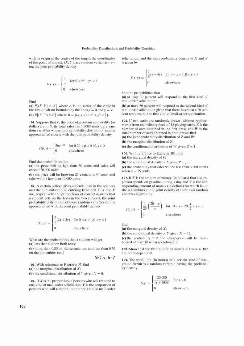
Probability Distributions and Probability Densities
with its origin at the center of the target, the coordinatesof the point of impact, (X, Y), are random variables hav-ing the joint probability density
f (x, y) =
1
πfor 0< x2+ y2< 1
0 elsewhere
Find(a) P[(X, Y) ∈ A], where A is the sector of the circle inthe first quadrant bounded by the lines y = 0 and y = x;
(b) P[(X, Y) ∈ B], where B = {(x, y)|0< x2+ y2< 12 }.
101. Suppose that P, the price of a certain commodity (indollars), and S, its total sales (in 10,000 units), are ran-dom variables whose joint probability distribution can beapproximated closely with the joint probability density
f (p, s) =
{
5pe−ps for 0.20<p< 0.40, s> 0
0 elsewhere
Find the probabilities that(a) the price will be less than 30 cents and sales willexceed 20,000 units;
(b) the price will be between 25 cents and 30 cents andsales will be less than 10,000 units.
102. A certain college gives aptitude tests in the sciencesand the humanities to all entering freshmen. If X and Yare, respectively, the proportions of correct answers thata student gets on the tests in the two subjects, the jointprobability distribution of these random variables can beapproximated with the joint probability density
f (x, y) =
2
5(2x+ 3y) for 0< x< 1, 0< y< 1
0 elsewhere
What are the probabilities that a student will get(a) less than 0.40 on both tests;
(b) more than 0.80 on the science test and less than 0.50on the humanities test?
SECS. 6–7
103. With reference to Exercise 97, find(a) the marginal distribution of X;
(b) the conditional distribution of Y given X = 0.
104. If X is the proportion of persons who will respond toone kind of mail-order solicitation, Y is the proportion ofpersons who will respond to another kind of mail-order
solicitation, and the joint probability density of X and Yis given by
f (x, y) =
2
5(x+ 4y) for 0< x< 1, 0< y< 1
0 elsewhere
find the probabilities that(a) at least 30 percent will respond to the first kind ofmail-order solicitation;
(b) at most 50 percent will respond to the second kind ofmail-order solicitation given that there has been a 20 per-cent response to the first kind of mail-order solicitation.
105. If two cards are randomly drawn (without replace-ment) from an ordinary deck of 52 playing cards, Z is thenumber of aces obtained in the first draw, and W is thetotal number of aces obtained in both draws, find(a) the joint probability distribution of Z and W;
(b) the marginal distribution of Z;
(c) the conditional distribution of W given Z = 1.
106. With reference to Exercise 101, find(a) the marginal density of P;
(b) the conditional density of S given P = p;
(c) the probability that sales will be less than 30,000 unitswhen p = 25 cents.
107. If X is the amount of money (in dollars) that a sales-person spends on gasoline during a day and Y is the cor-responding amount of money (in dollars) for which he orshe is reimbursed, the joint density of these two randomvariables is given by
f (x, y) =
1
25
(
20− x
x
)
for 10< x< 20,x
2< y< x
0 elsewhere
find(a) the marginal density of X;
(b) the conditional density of Y given X = 12;
(c) the probability that the salesperson will be reim-bursed at least $8 when spending $12.
108. Show that the two random variables of Exercise 102are not independent.
109. The useful life (in hours) of a certain kind of inte-grated circuit is a random variable having the probabil-ity density
f (x) =
20,000
(x+ 100)3for x> 0
0 elsewhere
)(&

Probability Distributions and Probability Densities
If three of these circuits operate independently, find(a) the joint probability density of X1, X2, and X3, repre-senting the lengths of their useful lives;
(b) the value of P(X1< 100, X2< 100, X3 G 200).
SEC. 8
110. The following are the percentages of tin in measure-ments made on 24 solder joints:
61 63 59 54 65 60 62 61 67 60 55 68
57 64 65 62 59 59 60 62 61 63 58 61
(a) Construct a stem-and-leaf diagram using 5 and 6 asthe stem labels.
(b) Construct a double-stem display.
(c) Which is more informative?
111. Suppose the first row of 12 observations in Exer-cise 110 came from solder connections made at station105 and the second row came from station 107. Use apair of stem-and-leaf diagrams to determine whether youshould suspect a difference in the soldering process at thetwo stations.
112. Two different lathes turn shafts to be used in electricmotors. Measurements made of their diameters (in cm)are
Lathe A: 1.42 1.38 1.40 1.41 1.39 1.44 1.36 1.42 1.40
Lathe B: 1.47 1.31 1.56 1.33 1.29 1.46 1.28 1.51
Construct two stem-and-leaf diagrams to see if youshould suspect that the two lathes are turning out shaftsof different diameters.
113. Use MINITAB or some other computer software toconstruct a stem-and-leaf display for the following datarepresenting the time to make coke (in hours) in succes-sive runs of a coking oven.
7.8 9.2 6.4 8.2 7.6 5.9 7.4 7.1 6.7 8.5
10.1 8.6 7.7 5.9 9.3 6.4 6.8 7.9 7.2 10.2
6.9 7.4 7.8 6.6 8.1 9.5 6.4 7.6 8.4 9.2
114. Use MINITAB or some other computer software toconstruct a stem-and-leaf display for the combined dataof Exercise 112.
115. The following are the drying times (minutes) of 100sheets coated with polyurethane under various ambientconditions:
45.6 50.3 55.1 63.0 58.2 65.5 51.1 57.4 60.4 54.9
56.1 62.1 43.5 63.8 64.9 59.9 63.0 67.7 53.8 57.9
61.8 52.2 61.2 51.6 58.6 73.8 53.9 64.1 57.2 75.4
55.9 70.1 46.2 63.6 56.0 48.1 62.2 58.8 50.8 68.1
51.4 73.9 66.7 42.9 71.0 56.1 60.8 58.6 70.6 62.2
59.9 47.5 72.5 62.0 56.8 54.3 61.0 66.3 52.6 63.5
64.3 63.6 53.5 55.1 62.8 63.3 64.7 54.9 54.4 69.6
64.2 59.3 60.6 57.1 68.3 46.7 73.7 56.8 62.9 58.4
68.5 68.9 62.1 62.8 74.4 43.8 40.0 64.4 50.8 49.9
55.8 66.8 67.0 64.8 57.6 68.3 42.5 64.4 48.3 56.5
Construct a frequency distribution of these data, usingeight classes.
116. Eighty pilots were tested in a flight simulator andthe time for each to take corrective action for a givenemergency was measured in seconds, with the followingresults:
11.1 5.2 3.6 7.6 12.4 6.8 3.8 5.7 9.0 6.0 4.9 12.6
7.4 5.3 14.2 8.0 12.6 13.7 3.8 10.6 6.8 5.4 9.7 6.7
14.1 5.3 11.1 13.4 7.0 8.9 6.2 8.3 7.7 4.5 7.6 5.0
9.4 3.5 7.9 11.0 8.6 10.5 5.7 7.0 5.6 9.1 5.1 4.5
6.2 6.8 4.3 8.5 3.6 6.1 5.8 10.0 6.4 4.0 5.4 7.0
4.1 8.1 5.8 11.8 6.1 9.1 3.3 12.5 8.5 10.8 6.5 7.9
6.8 10.1 4.9 5.4 9.6 8.2 4.2 3.4
Construct a frequency distribution of these data.
117. Find the class boundaries, the class interval, and theclass marks of the frequency distribution constructed inExercise 115.
118. Find the class boundaries, the class interval, and theclass marks of the frequency distribution constructed inExercise 116.
119. The following are the number of highway accidentsreported on 30 successive days in a certain county:
6 4 0 3 5 6 2 0 0 12 3 7 2 1 1
0 4 0 0 0 1 8 0 2 4 7 3 6 2 0
Construct a frequency distribution of these data. Iden-tify the class boundaries, the class marks, and the classinterval.
120. A percentage distribution is obtained from a fre-quency distribution by replacing each frequency by 100times the ratio of that frequency to the total frequency.Construct a percentage distribution using the reaction-time data of Exercise 116.
)('

Probability Distributions and Probability Densities
121. Construct a percentage distribution using the drying-time data of Exercise 115.
122. Percentage distributions are useful in comparing twofrequency distributions having different total frequen-cies. Construct percentage distributions from the follow-ing two frequency distributions and determine whetherthe distributions of daily absences in the two departmentsfollow similar patterns.
FREQUENCIES
Class Shipping SecurityLimits Department Department
0–1 26 18
2–3 18 11
4–5 10 7
6–7 4 3
8–9 2 1
Totals 60 40
123. A cumulative frequency distribution is constructedfrom a frequency distribution by replacing each fre-quency with the sum of the frequency of the given classand the frequencies of all classes above it, and represent-ing each class by its upper class boundary. Construct acumulative frequency distribution using the data of Exer-cise 115.
124. Construct a cumulative frequency distribution usingthe data of Exercise 116.
125. Construct cumulative percentage distributions fromthe frequency distributions of absences given in Exer-cise 122.
126. Unequal class intervals. The small number of obser-vations greater than 7 in Exercise 119 may cause somedifficulty in constructing a frequency distribution. Tokeep class intervals equal, one is faced with the dilemmaof either creating too many classes for only 30 observa-tions or using a small number of classes with excessiveloss of information in the first few classes. In such cases,one is tempted to drop the rule of equal-size classes, usinga larger interval for the last class.(a) If that were done, what would the resulting frequencydistribution become?
(b) Is there a unique class interval?
127. The following are the times to failure of 38 lightbulbs, given in hours of operation.
150 389 345 310 20 310 175 376 334 340
332 331 327 344 328 341 325 2 311 320
256 315 55 345 111 349 245 367 81 327
355 309 375 316 336 278 396 287
(a) Dropping the rule that class intervals must be equal,construct a frequency distribution from these data.
(b) Can you find the class mark of every class?
128. (a) Construct a histogram of the reaction times ofpilots from the data in Exercise 116.
(b) What can be said about the shape of this histogram?
129. (a) Construct a histogram of the drying times ofpolyurethane from the data in Exercise 115.
(b) What can be said about the shape of this histogram?
130. Use the data of Exercise 128 to illustrate that classmarks are given by the midpoint between successive classboundaries as well as the midpoint between successiveclass limits.
131. Using the data of Exercise 129, show that the classmarks also are given by the midpoint between successiveclass boundaries.
132. Construct a histogram using the solder-joint data inExercise 110.
133. (a) Using only the first two rows of the data for theresponse times given in Section 8, construct a histogram.
(b) How would you describe the shape of the histogram?
134. (a) Combining the data for both lathes in Exer-cise 112, construct a histogram.
(b) How would you describe the shape of the histogram?
135. Use MINITAB or some other computer software toconstruct a histogram of the coking-time data given inExercise 113.
136. Use MINITAB or some other computer software toconstruct a histogram of the drying-time data in Exer-cise 115.
137. A plot of the points (x, f ), where x represents theclass mark of a given class in a frequency distribution andf represents its frequency, is called a frequency polygon.Construct a frequency polygon using the data in Exer-cise 116.
138. Construct a frequency polygon from the data inExercise 115.
139. A plot of the cumulative frequency (see Exer-cise 123) on the y-axis and the corresponding upper classboundary on the x-axis is called an ogive.
))(

Probability Distributions and Probability Densities
(a) Construct an ogive for the data of Exercise 115.
(b) Using the same set of axes, relabel the y-axis so thatthe same graph also shows the ogive of the percentagedistribution of drying times.
140. (a) Construct an ogive for the reaction times givenin Exercise 116.
(b) Construct an ogive representing the cumulative per-centage distribution.
References
More advanced or more detailed treatments of the mate-rial in this chapter may be found in
Brunk, H. D., An Introduction to Mathematical Statistics,3rd ed. Lexington, Mass.: Xerox College Publishing,1975,
DeGroot, M. H., Probability and Statistics, 2nd ed. Read-ing, Mass.: Addison-Wesley Publishing Company, Inc.,1986,
Fraser, D. A. S., Probability and Statistics: Theory andApplications. North Scituate, Mass.: Duxbury Press,1976,
Hogg, R. V., and Craig, A. T., Introduction to Mathemat-ical Statistics, 4th ed. New York: Macmillan PublishingCo., Inc., 1978,
Kendall, M. G., and Stuart, A., The Advanced Theoryof Statistics, Vol. 1, 4th ed. New York: Macmillan Pub-lishing Co., Inc., 1977,
Khazanie, R., Basic Probability Theory and Applica-tions. Pacific Palisades, Calif.: Goodyear PublishingCompany, Inc., 1976.
Answers to Odd-Numbered Exercises
1 (a) no, because f (4) is negative; (b) yes; (c) no, becausethe sum of the probabilities is less than 1.
5 0<k< 1.
9 (a) no, because F(4) exceeds 1; (b) no, because F(2) isless than F(1); (c) yes.
11 (a) 12 ; (b) 1
6 ; (c) f (1) = 13 ; f (4) = 1
6 ; f (6) = 23 ;
f (10) = 16 ; f (x) = 0 elsewhere.
13 (a) 34 ; (b) 1
4 ; (c) 12 ; (d) 3
4 ; (e) 12 ; (f) 1
4 .
17 (b) 25 .
19 (c) 0.124.
21 F(y) =
0 for y… 2
116 (y
2+ 2y− 8) for 2< y< 4
1 for yÚ 4
The probabilities are 0.454 and 0.1519.
23 F(x) =
0 for x… 012
√x for 0< x< 4;
1 for xÚ 4
(b) 14 and 1
2 .
25 F(z) =
{
0 for z… 0
1− e−z2for z> 0
27 G(x) =
0 for x… 0
3x2− 2x3 for 0< x< 1
1 for xÚ 1
The probabilities are 532 and 1
2 .
29 F(x) =
0 for x… 0
x2
2for 0< x< 1
2x−x2
2− 1 for … x< 2
1 for xÚ 2
31 F(x) =
0 for x… 0
x2
4for 0< x… 1
14 (2x− 1) for 1< x… 2
14 (6x− x2− 5) for 2< x< 3
1 for xÚ 3
33 f (x) = 12 for − 1< x< 1 and f (x) = 0 elsewhere.
35 f (y) =18
y3for y> 0 and f (y) = 0 elsewhere; the two prob-
abilities are 1625 and 9
64 .
37 The three probabilities are 1− 3e−2, 2e−1− 4e−3, and
5e−5.
39 (a) F(x) = 0; (b) F(x) = 12 x; (c) F(x) = 1
2 (x+ 1);(d) F(x) = 0.
41 The probabilities are 14 , 1
4 , 38 , and 1
2 .
43 (a) 14 ; (b) 0; (c) 7
24 ; (d) 119120 .
45 (a) 2989 ; (b) 5
89 ; (c) 5589 .
)))
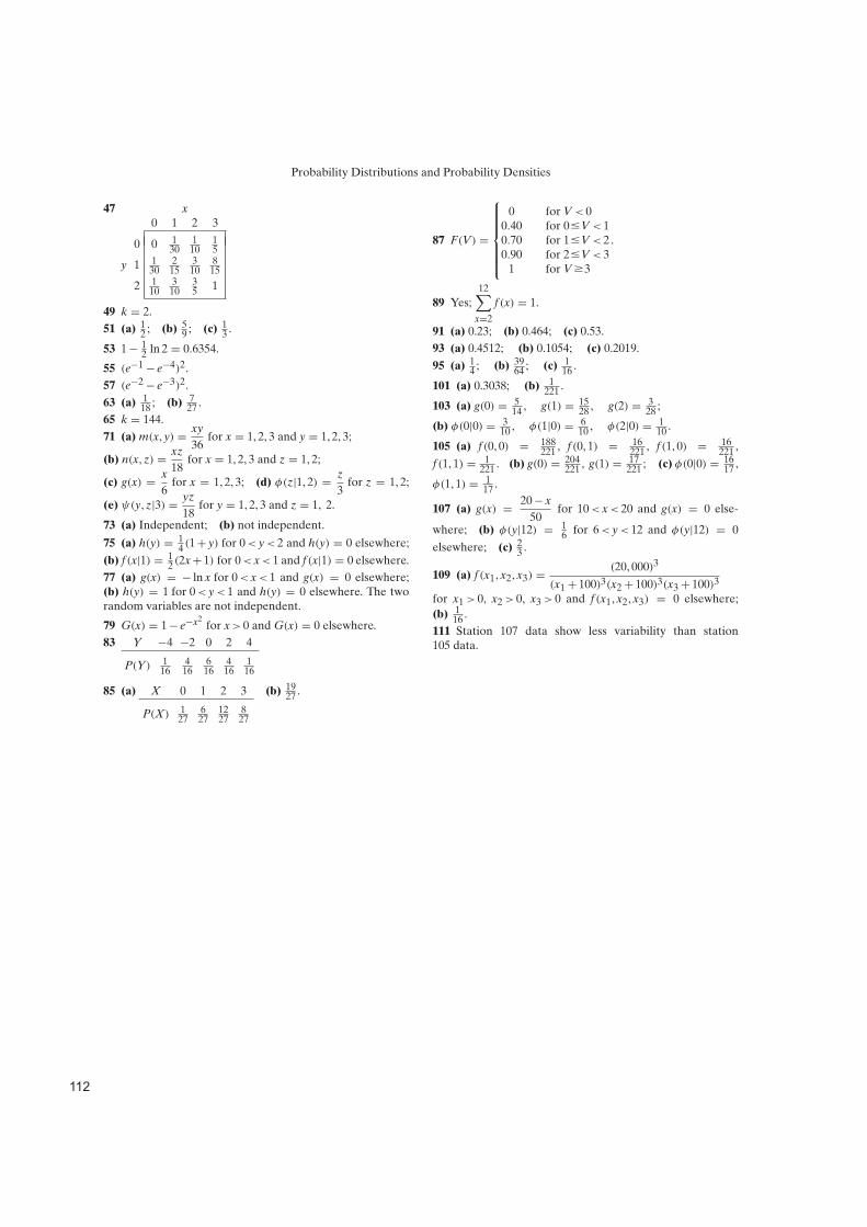
Probability Distributions and Probability Densities
47 x
0 1 2 3
0 0 130
110
15
y 1 130
215
310
815
2 110
310
35 1
49 k = 2.
51 (a) 12 ; (b) 5
9 ; (c) 13 .
53 1− 12 ln 2 = 0.6354.
55 (e−1− e−4)2.
57 (e−2− e−3)2.
63 (a) 118 ; (b) 7
27 .
65 k = 144.
71 (a) m(x, y) =xy
36for x = 1, 2, 3 and y = 1, 2, 3;
(b) n(x, z) =xz
18for x = 1, 2, 3 and z = 1, 2;
(c) g(x) =x
6for x = 1, 2, 3; (d) φ(z|1, 2) =
z
3for z = 1, 2;
(e) ψ(y, z|3) =yz
18for y = 1, 2, 3 and z = 1, 2.
73 (a) Independent; (b) not independent.
75 (a) h(y) = 14 (1+ y) for 0< y< 2 and h(y) = 0 elsewhere;
(b) f (x|1) = 12 (2x+ 1) for 0< x< 1 and f (x|1) = 0 elsewhere.
77 (a) g(x) = − ln x for 0< x< 1 and g(x) = 0 elsewhere;(b) h(y) = 1 for 0< y< 1 and h(y) = 0 elsewhere. The tworandom variables are not independent.
79 G(x) = 1− e−x2for x> 0 and G(x) = 0 elsewhere.
83 Y −4 −2 0 2 4
P(Y) 116
416
616
416
116
85 (a) X 0 1 2 3
P(X) 127
627
1227
827
(b) 1927 .
87 F(V) =
0 for V< 00.40 for 0…V< 10.70 for 1…V< 20.90 for 2…V< 3
1 for V Ú 3
.
89 Yes;
12∑
x=2
f (x) = 1.
91 (a) 0.23; (b) 0.464; (c) 0.53.
93 (a) 0.4512; (b) 0.1054; (c) 0.2019.
95 (a) 14 ; (b) 39
64 ; (c) 116 .
101 (a) 0.3038; (b) 1221 .
103 (a) g(0) = 514 , g(1) = 15
28 , g(2) = 328 ;
(b) φ(0|0) = 310 , φ(1|0) = 6
10 , φ(2|0) = 110 .
105 (a) f (0, 0) = 188221 , f (0, 1) = 16
221 , f (1, 0) = 16221 ,
f (1, 1) = 1221 . (b) g(0) = 204
221 , g(1) = 17221 ; (c) φ(0|0) = 16
17 ,
φ(1, 1) = 117 .
107 (a) g(x) =20− x
50for 10< x< 20 and g(x) = 0 else-
where; (b) φ(y|12) = 16 for 6< y< 12 and φ(y|12) = 0
elsewhere; (c) 23 .
109 (a) f (x1, x2, x3) =(20, 000)3
(x1+ 100)3(x2+ 100)3(x3+ 100)3
for x1> 0, x2> 0, x3> 0 and f (x1, x2, x3) = 0 elsewhere;
(b) 116 .
111 Station 107 data show less variability than station105 data.
!