26 June 2016

BACHELOR ASSIGNMENT

FREQUENCY TAGGING OFELECTROCUTANEOUS STIMULIFOR OBSERVATION OF CORTICALNOCICEPTIVE PROCESSING

S.F.J. Nijhofs1489488

Faculty of Electrical Engineering, Mathematics and Computer Science (EEMCS)Biological Signals and Systems (BSS)

Exam committee:J. BuitenwegT. HeidaW. Olthuis

Summary

Research on nociceptive (pain related) processing in the human nervous system is requiredto improve treatment for chronic pain patients. A key characteristic of chronic pain is develop-ment of maladaptive nociceptive processing. If these changes could be detected in an earlystage, more accurate treatment could be given and would yield better results and less clinicaleffort per patient. Diagnostic methods are useful for characterizing the processing of nocicept-ive information. Observation methods have been developed already to measure responses tophasic stimuli applied to the peripheral nervous system. In combination with EEG measure-ments, more objective information can be obtained. Previous methods show good results inobservation of neural responses to stimuli. This would be improved by an possibility to meas-ure neural measurements of longer durations.

New investigations are carried out aimed to evaluate responses of longer lasting tonic stim-uli. ’Frequency tagging’ is a method that could be used for this. With frequency tagging, apulse train of several seconds with pulses in the millisecond range is modulated on and off witha certain specified frequency. The goal of applying stimuli with this pattern is to see this samemodulation frequency back in measurements of specific activated places in the bran corres-ponding to nociceptive processing. In this assignment, frequency tagging is implemented ona setup that was able to send phasic stimuli only. Key factor in the design of this setup is thestrict timing requirement for generation of accurate frequencies. Properties related with timingare first evaluated, thereafter a validation experiment of the entire setup was performed. Thisvalidation experiment was done on a human subject. A relative nociceptive threshold was de-termined by applying pulse trains with increasing amplitude while measuring reactions. Afterthe threshold was determined, the pulse train amplitude was set to twice this value to generatea definite pain sensation. Pulse trains with modulation frequencies of 13, 20, 33 and 43 Hzwere applied and EEG was measured. Phase locked and non phase locked analysis in timeand frequency domain was performed to interpret the data.

Results show that frequency content corresponding to the input signal can be found back inthe EEG measurements. Specific sharp peaks are observed in the frequency-magnitude plotof EEG channel derivations. Frequencies at which these peaks occurred where higher har-monics and combinations of the modulation frequency and frequency corresponding to singlepulse timing. Phasic responses were found at the onset of pulse trains. Frequency content atthe modulation frequency was only found for 33 Hz. For all other modulation frequencies, thefundamental frequency could not be observed clearly. Evaluating at 50 ms time around stim-ulus onset specifically, it was found that frequency content corresponding to the input signalwas measured in EEG signals before human responses were possible. This is an indication ofstimulus artifacts in the measurements.

Due to the presence of stimulus artifacts in measurement data, the findings cannot yet contrib-ute to characterizations of nociceptive processing. The setup is able to generate and measureaccurate frequency components, however due to the presence of stimulus artifacts these fre-quencies cannot be clearly separated as measurements of nociceptive processing solely. Thecause of stimulus artifacts is not yet fully understood. This could be dependent on voltageglitches in the output of the stimulator.

i

Abbreviations

EEG Electroencephalography

ES Electrical stimulation

DFT Discrete Fourier transform

FFT Fast Fourier transform

fMRI Functional magnetic resonance imaging

IES Intra-epidermal stimulation

IPI Inter pulse interval

MEG Magnetoencephalography

MWT Morlet wavelet transform

NoP Number of pulses

LS Laser stimulation

PET Positron emission tomography

PSD Power spectral density

PW Pulse width

ii

Contents

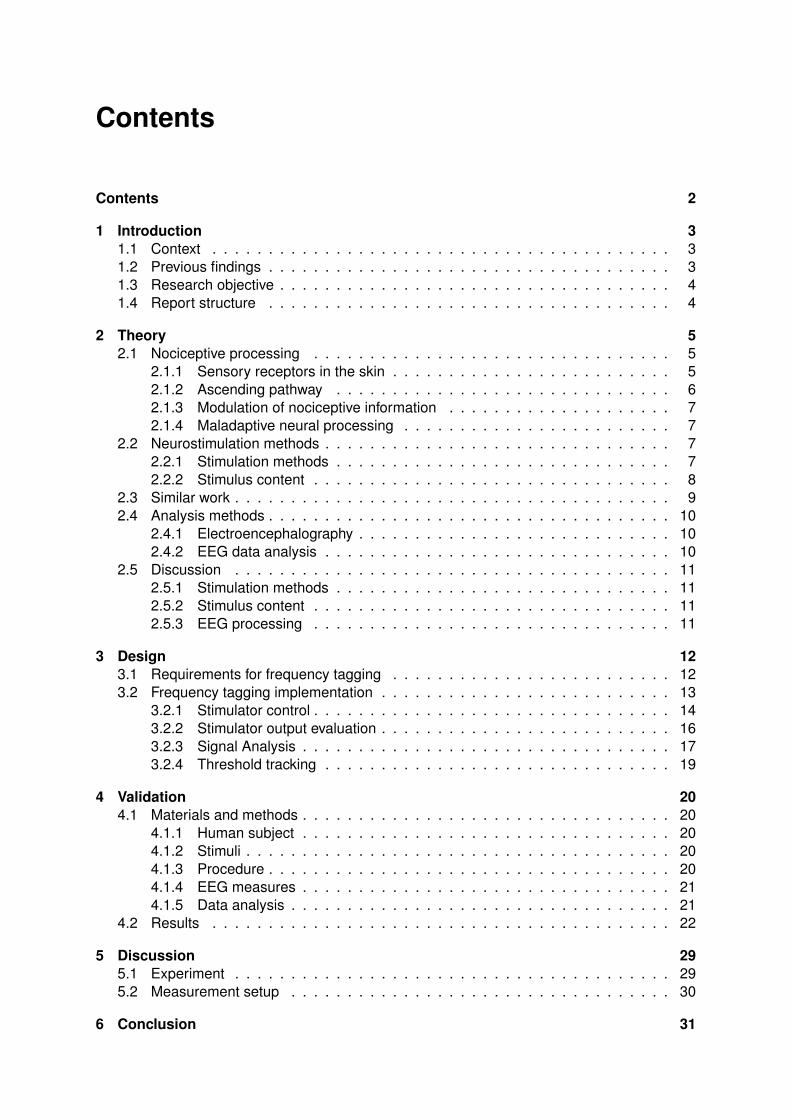
Contents 2

1 Introduction 31.1 Context . . . . . . . . . . . . . . . . . . . . . . . . . . . . . . . . . . . . . . . . . 31.2 Previous findings . . . . . . . . . . . . . . . . . . . . . . . . . . . . . . . . . . . . 31.3 Research objective . . . . . . . . . . . . . . . . . . . . . . . . . . . . . . . . . . . 41.4 Report structure . . . . . . . . . . . . . . . . . . . . . . . . . . . . . . . . . . . . 4

2 Theory 52.1 Nociceptive processing . . . . . . . . . . . . . . . . . . . . . . . . . . . . . . . . 5

2.1.1 Sensory receptors in the skin . . . . . . . . . . . . . . . . . . . . . . . . . 52.1.2 Ascending pathway . . . . . . . . . . . . . . . . . . . . . . . . . . . . . . 62.1.3 Modulation of nociceptive information . . . . . . . . . . . . . . . . . . . . 72.1.4 Maladaptive neural processing . . . . . . . . . . . . . . . . . . . . . . . . 7

2.2 Neurostimulation methods . . . . . . . . . . . . . . . . . . . . . . . . . . . . . . . 72.2.1 Stimulation methods . . . . . . . . . . . . . . . . . . . . . . . . . . . . . . 72.2.2 Stimulus content . . . . . . . . . . . . . . . . . . . . . . . . . . . . . . . . 8

2.3 Similar work . . . . . . . . . . . . . . . . . . . . . . . . . . . . . . . . . . . . . . . 92.4 Analysis methods . . . . . . . . . . . . . . . . . . . . . . . . . . . . . . . . . . . . 10

2.4.1 Electroencephalography . . . . . . . . . . . . . . . . . . . . . . . . . . . . 102.4.2 EEG data analysis . . . . . . . . . . . . . . . . . . . . . . . . . . . . . . . 10

2.5 Discussion . . . . . . . . . . . . . . . . . . . . . . . . . . . . . . . . . . . . . . . 112.5.1 Stimulation methods . . . . . . . . . . . . . . . . . . . . . . . . . . . . . . 112.5.2 Stimulus content . . . . . . . . . . . . . . . . . . . . . . . . . . . . . . . . 112.5.3 EEG processing . . . . . . . . . . . . . . . . . . . . . . . . . . . . . . . . 11

3 Design 123.1 Requirements for frequency tagging . . . . . . . . . . . . . . . . . . . . . . . . . 123.2 Frequency tagging implementation . . . . . . . . . . . . . . . . . . . . . . . . . . 13

3.2.1 Stimulator control . . . . . . . . . . . . . . . . . . . . . . . . . . . . . . . . 143.2.2 Stimulator output evaluation . . . . . . . . . . . . . . . . . . . . . . . . . . 163.2.3 Signal Analysis . . . . . . . . . . . . . . . . . . . . . . . . . . . . . . . . . 173.2.4 Threshold tracking . . . . . . . . . . . . . . . . . . . . . . . . . . . . . . . 19

4 Validation 204.1 Materials and methods . . . . . . . . . . . . . . . . . . . . . . . . . . . . . . . . . 20

4.1.1 Human subject . . . . . . . . . . . . . . . . . . . . . . . . . . . . . . . . . 204.1.2 Stimuli . . . . . . . . . . . . . . . . . . . . . . . . . . . . . . . . . . . . . . 204.1.3 Procedure . . . . . . . . . . . . . . . . . . . . . . . . . . . . . . . . . . . . 204.1.4 EEG measures . . . . . . . . . . . . . . . . . . . . . . . . . . . . . . . . . 214.1.5 Data analysis . . . . . . . . . . . . . . . . . . . . . . . . . . . . . . . . . . 21

4.2 Results . . . . . . . . . . . . . . . . . . . . . . . . . . . . . . . . . . . . . . . . . 22

5 Discussion 295.1 Experiment . . . . . . . . . . . . . . . . . . . . . . . . . . . . . . . . . . . . . . . 295.2 Measurement setup . . . . . . . . . . . . . . . . . . . . . . . . . . . . . . . . . . 30

6 Conclusion 31

6.1 Conclusions . . . . . . . . . . . . . . . . . . . . . . . . . . . . . . . . . . . . . . . 316.2 Recommendations . . . . . . . . . . . . . . . . . . . . . . . . . . . . . . . . . . . 31

7 Acknowledgments 33

A Stimulator output calibration 36

B Fourier series analysis 40

C Subject information letter 44

D Analysis focused on stimulus onset 46

1. Introduction

1.1 Context

Annually 150.000 to 200.000 patients suffer from chronic pain in the Netherlands. Once aperson has chronic pain, relatively ineffective treatment is performed. To make treatment bet-ter, diagnostics and therapeutic measures in an early stage would result in better treatmentoutcome and less clinical effort per patient. Chronic pain is often the result of disturbed pro-cesses in the central nervous system. An increased sensitivity to noxious stimuli (generalizedhyperalgesia) is widely recognized as key factor in chronic pain development. Nociceptivestimuli are processed by neural mechanisms at several places in an ascending pathway fromthe peripheral nervous system to the brain, resulting into conscious experience of pain. Theascending processing is modulated by descending pathways. Due to injury or disease, mal-adaptive changes in both ascending and descending pathways may result in increased painsensitivity. Clinical observation methods of maladaptive processing are limited at this moment,but if insight would be increased this would permit better understanding and early detection ofchronic pain.

1.2 Previous findings

Different observation methods of nociceptive processing exist. One developed observationmethod uses phasic electrocutaneous stimulation of nociceptors to generate pain experience.Electrical current stimuli with varying number of pulses, amplitude and inter pulse intervals areapplied. These different temporal stimulus properties result in different reactions of nociceptiveprocessing mechanisms, measured by conscious perception of pain. This perception could forinstance be the push of a button or a subjective rating on a scale. An analysis of stimulus-response pairs results in estimated nociceptive detection thresholds of multiple stimulus types.This provides information about the properties of nociceptive mechanisms. During a thresholdtracking experiment, electroencephalography (EEG) measurements from the scalp are addedto gain additional objective information about nociceptive processing in the brain. Due to thephasic nature of the stimuli, observable responses in the EEG can be separated from spon-taneous activities in the brain by using time locked analysis techniques, e.g. averaging in time.

Applying abrupt stimuli with a phasic nature is a method for observing brain responses, how-ever this is less representative for visualizing processing pathways of nociceptive information.An alternative approach would be applying tonic stimuli of longer duration, however time lockedanalysis techniques are not applicable here. This requires an alternative method to separatestimulation responses and spontaneous activities in the brain. ’Frequency tagging’ has beenproposed as a method. Here, tonic stimuli with a controlled frequency are applied where afterthe frequency content of the stimuli should be observable in EEG recordings of the brain. Sucha method could be helpful for analysis of tonic stimuli and therefore the study of nociceptiveprocessing pathways.

3

1.3 Research objective

The goal of this bachelor assignment is to implement a frequency tagging measurement setup.Hardware of an existing nociceptive threshold tracking setup will be used as a starting point.This can be extended with different software while hardware can be kept the same. After im-plementation of the setup, a first experiment will be carried out in such a way that a preliminarydata analysis can be executed. Results could then be used as a validation method for theextension of the measurement setup. If the setup would be correct, results could also be usedfor characterization of nociceptive processing pathways.

1.4 Report structure

This report will contain a a literature study in chapter 2. This will include a description ofnociceptive information processing in the human body, methods to stimulate nociceptive re-ceptors, analysis and measurement of cortical activity and findings of previous research cov-ering frequency tagging of nociceptive information. Chapter 3 will describe the previous setup,requirements for frequency tagging and implementation of frequency tagging. The implement-ation is also validated in this chapter. Chapter 4 describes an evaluation experiment of thetotal setup and corresponding results. The results of this validation experiment and the im-plemented setup will be discussed in chapter 5. Chapter 6 concludes this research and givesrecommendations for future related work.

4

2. Theory

In order to design a device which is intended to characterize the human body, it is necessary toknow what needs to be characterized. Therefore, a literature study on nociceptive processingin the human body will be needed. To be able to present stimuli to and obtain responsesfrom the human body it has to be known which methods are available, therefore the literaturestudy will cover neurostimulation methods and EEG analysis methods as well. Methodologiesand results of previous work covering frequency tagging of nociceptive pathways will also bediscussed to generate initial sense of the methodology.

2.1 Nociceptive processing

One of the functions of the nervous system is managing transport of signals to different partsin the body. Sense and motor organs are all connected with the nervous system in the humanbody to send and receive signals. One type of sense organs in the skin are nociceptors.Nociceptors are spread over the whole body and are responsible for sensing pain. Signalsoriginating from these receptors are processed in an ascending pathway via afferent nervefibers in the peripheral nervous system, laminae in the spinal cord, centers in the brainstemand thalamus to the primary somatosensory cortex in the brain. Different descending pathwaysexist as well, these have ability to modulate the ascending pathway signal transmission. Sincenociceptive processing will be discussed superficially here, main reasoning in this section isfollowed from introductory text books from Purves et al. [1] and Noback et al. [2]. As anelectrical engineering student, this is not general accepted knowledge but for persons with amedical background it should be.

2.1.1 Sensory receptors in the skin

There are different types of sensory receptors in the skin, based on function they can be cat-egorized into three groups: mechanoreceptors, nociceptors and thermoceptors [1]. Mechanor-eceptors are mainly in the deeper layers of the skin. Nociceptors and thermoceptors can alsobe found in the upper regions of the skin. This is because both receptors are different types.Nociceptors and thermoceptors are free nerve endings and mechanoceptors have specificreceptor elements. The free nerve endings are branches from neurons and can convert stim-ulation directly into action potentials. If a nerve ending is stimulated, the permeability of thecell membrane is changed. This results in a depolarizing current going to the central nervoussystem. Strength of a stimulus is non linearly related to different rates of action potential thatare generated by receptors. This process is different per type of receptor. Due to difference perreceptor, information can reach the brain quick if a strong stimulus is present and informationcan reach the brain when a stimulus is going on for a longer time. Phasic receptors can adapttheir output relatively fast and respond with a maximal rate of action potentials for a short timeand tonic receptors adapt their output slower but keep firing at a lower rate and keep going fora longer time. Nociceptive receptors can be seen as tonic receptors.

Neurons of free nerves are centered in dorsal root ganglia. They have two axons, one go-ing to the spinal cord or brainstem and another one going to nerve endings in the peripheralnervous system. Axons associated with nociceptive nerve endings are either bundled in un-myelinated C-fibers or lightly myelinated Aδ-fibers. More myelination causes faster conduction

5

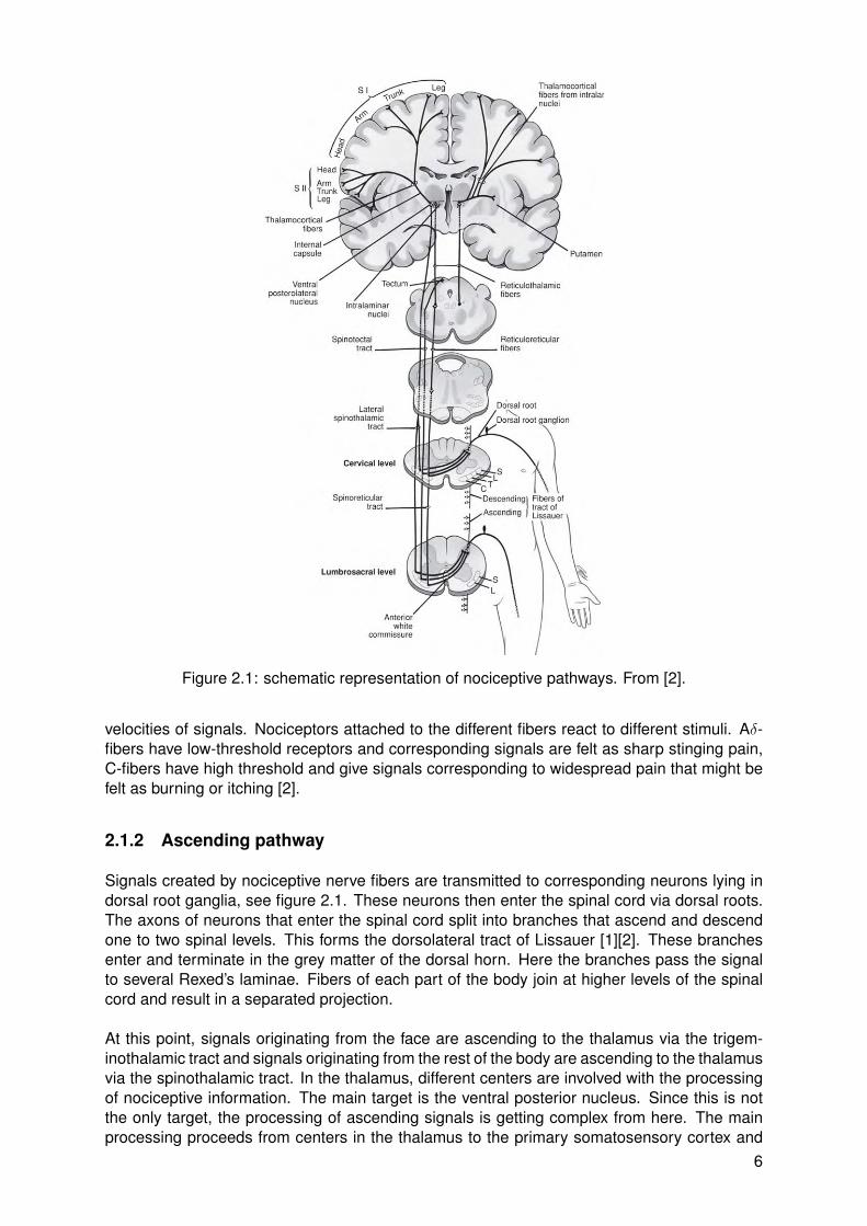
Figure 2.1: schematic representation of nociceptive pathways. From [2].

velocities of signals. Nociceptors attached to the different fibers react to different stimuli. Aδ-fibers have low-threshold receptors and corresponding signals are felt as sharp stinging pain,C-fibers have high threshold and give signals corresponding to widespread pain that might befelt as burning or itching [2].

2.1.2 Ascending pathway

Signals created by nociceptive nerve fibers are transmitted to corresponding neurons lying indorsal root ganglia, see figure 2.1. These neurons then enter the spinal cord via dorsal roots.The axons of neurons that enter the spinal cord split into branches that ascend and descendone to two spinal levels. This forms the dorsolateral tract of Lissauer [1][2]. These branchesenter and terminate in the grey matter of the dorsal horn. Here the branches pass the signalto several Rexed’s laminae. Fibers of each part of the body join at higher levels of the spinalcord and result in a separated projection.

At this point, signals originating from the face are ascending to the thalamus via the trigem-inothalamic tract and signals originating from the rest of the body are ascending to the thalamusvia the spinothalamic tract. In the thalamus, different centers are involved with the processingof nociceptive information. The main target is the ventral posterior nucleus. Since this is notthe only target, the processing of ascending signals is getting complex from here. The mainprocessing proceeds from centers in the thalamus to the primary somatosensory cortex and

6

secondary somatosensory cortex. Nociceptive information in these areas is thought to beidentifying location and intensity of pain as well as quality of the stimulation [1]. Other areas inthe brain are responsible for psychological modulation of pain perception. The insular cortexand anterior cingulate cortex are involved with judging the intensity of pain [3][4].

2.1.3 Modulation of nociceptive information

Nociceptive information that ascends to cortices is modulated by descending signals whichcan both inhibit or facilitate the sensitivity of nociceptors and processing centers of pain inthe central nervous system. Signals can originate from the somatosensory cortex, amygdalaand hypothalamus and go to the periaqueductal grey in the midbrain in the brainstem [1][5].Stimulation of the periaqueductal grey is processed via different centers in the brainstem to thedescending pathways in the spinal cord. The different centers in the brainstem are respons-ible for generating multiple different neurotransmitters which can have positive and negativeeffects. These neurotransmitters affect descending pathways in the spinal cord as well as con-nections between ascending and descending pathways and synaptic terminals of nociceptiveafferents [1]. It is also possible for neural circuits within the dorsal grey in the spinal cord tomodulate information of nociceptive afferents such that higher centers already receive modu-lated information.

2.1.4 Maladaptive neural processing

There are a lot of ways in which the processing of nociceptive information can be affected andnot all of these are known. One of many consequences of maladaptive neural processing ischronic pain. This could be caused by changes in the working of descending modulation net-work [6], for instance due to an operation. Patients could have either an insufficient descendinginhibitory system or an enhanced descending facilitatory system. Since the descending path-way in the spinal cord is controlled by centers in the brainstem, it has been shown that differentcenters in the brainstem can have positive or negative effects on central sensitization and hy-peralgesia [6]. This results in an increased sensitivity and possible persistence of pain and arekey indicators for chronic pain.

2.2 Neurostimulation methods

2.2.1 Stimulation methods

In order to activate nociceptive processing, the body has to be stimulated. It is important thatsuch stimuli generate the same response of the nervous system as what would happen when anormal painful event occurs. It is also important that nociceptive nerves can be stimulated se-lectively in order to characterize pathways of nociceptive information separately from pathwaysof other non-nociceptive mechanisms. The purpose of stimulating the nerves is to measurenociceptive pathways. This means that a measured response should be linked to a certainstimulus. Such a relation between stimulus and response requires strict time requirements ofthe stimulator. For example, if stimuli are presented with a too slow increase of amplitude, itis not certain what provoked a response. Three different stimulation methods are describedhere: laser stimulation (LS), intra-epidermal stimulation (IES) and transcutaneous electricalstimulation (ES). The methods are schematically represented in figure 2.2 and explained fur-ther below.

First, nociceptors can be activated by laser stimulation (LS). Laser stimulation works by heat-ing the skin, which allows for activating heat-sensitive aδ- and C-fiber endings. It has beenshown that this can be done selectively [8]. Laser stimulation is very popular, since a laser can

7

Figure 2.2: schematic overview different stimulation methods. Laser stimulation (LS),intra-epidermal electrical stimulation (IES) and transcutaneous electrical stimulation (ES)are represented. Only Aδ and C nociceptive-free nerve endings can be found in the mostsuperficial layers of the skin. Non-nociceptive receptors are located deeper. From [7].

generate steep heating ramps which result in time-locked responses in the brain [9], howeveradditional time is required for heat conduction to the skin and transduction into a neural im-pulse. A disadvantage of laser stimulation is that time between two stimuli at the same locationshould be long (usually 5-20 seconds) and skin temperature cannot be controlled by solely thelaser [8].

Second, a method to activate nociceptors selectively is by intra-epidermal electrical stimulation(IES). This method is based on a separation between nociceptive receptors in the epidermisand non-nociceptive receptors in the dermis. Small currents spatially restricted to the epi-dermis are applied via a small flat needle. For low currents, only the epidermis is affected andIES is shown to be selective for Aδ-fibers [7]. Small currents might not be strong enough forgenerating a good perception or signal to noise ratio. Temporal summation can be used tocompensate for that. This is done by using short IES pulse trains, where longer pulse trainsresult in higher intensity of perception and higher amplitude of evoked potentials (EP) in thebrain [10][11].

Third, a crude stimulation method named transcutaneous electrical stimulation (ES) can beused. This method delivers a current to the epidermis and dermis, resulting in activation of non-nociceptive and nociceptive receptors. Most non-nociceptive receptors have lower thresholdsthan nociceptors [1]. This means that non-nociceptive are activated more if a stimulus is ap-plied. Due to activation of non-nociceptive receptors, this method is not selective for nocicept-ors and thus not suited for characterizing nociceptive pathways.

2.2.2 Stimulus content

The type of stimulus applied to nociceptors can be very different, as it can be used for multiplepurposes. Mostly, rectangular pulses are used to simulate pain. Previous research has beendone into variations of temporal properties of stimuli resulting in variations of evoked potentialsin cortices [12][13]. Temporal properties that can be made variable are pulse width (PW) andinter pulse interval (IPI), which is the time between the onsets of two pulses. A next step bey-ond looking at effects of temporal stimuli properties would be looking at effects of tonic stimuliresulting in steady state evoked potentials in cortices. Tonic stimuli are repeating patterns atcertain frequencies. The purpose of stimulating nociceptors with these frequencies is to seeif further nociceptive processing cortical areas contain these frequencies as well, indicating a

8

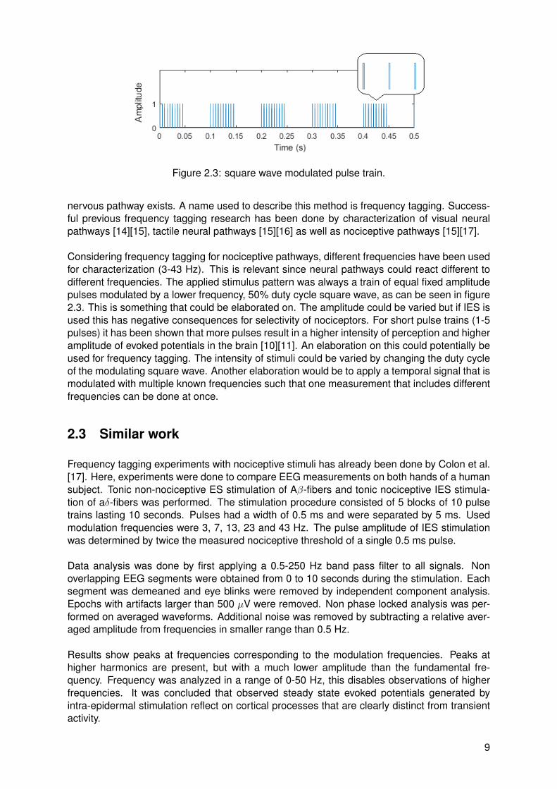
Figure 2.3: square wave modulated pulse train.

nervous pathway exists. A name used to describe this method is frequency tagging. Success-ful previous frequency tagging research has been done by characterization of visual neuralpathways [14][15], tactile neural pathways [15][16] as well as nociceptive pathways [15][17].

Considering frequency tagging for nociceptive pathways, different frequencies have been usedfor characterization (3-43 Hz). This is relevant since neural pathways could react different todifferent frequencies. The applied stimulus pattern was always a train of equal fixed amplitudepulses modulated by a lower frequency, 50% duty cycle square wave, as can be seen in figure2.3. This is something that could be elaborated on. The amplitude could be varied but if IES isused this has negative consequences for selectivity of nociceptors. For short pulse trains (1-5pulses) it has been shown that more pulses result in a higher intensity of perception and higheramplitude of evoked potentials in the brain [10][11]. An elaboration on this could potentially beused for frequency tagging. The intensity of stimuli could be varied by changing the duty cycleof the modulating square wave. Another elaboration would be to apply a temporal signal that ismodulated with multiple known frequencies such that one measurement that includes differentfrequencies can be done at once.

2.3 Similar work

Frequency tagging experiments with nociceptive stimuli has already been done by Colon et al.[17]. Here, experiments were done to compare EEG measurements on both hands of a humansubject. Tonic non-nociceptive ES stimulation of Aβ-fibers and tonic nociceptive IES stimula-tion of aδ-fibers was performed. The stimulation procedure consisted of 5 blocks of 10 pulsetrains lasting 10 seconds. Pulses had a width of 0.5 ms and were separated by 5 ms. Usedmodulation frequencies were 3, 7, 13, 23 and 43 Hz. The pulse amplitude of IES stimulationwas determined by twice the measured nociceptive threshold of a single 0.5 ms pulse.

Data analysis was done by first applying a 0.5-250 Hz band pass filter to all signals. Nonoverlapping EEG segments were obtained from 0 to 10 seconds during the stimulation. Eachsegment was demeaned and eye blinks were removed by independent component analysis.Epochs with artifacts larger than 500 µV were removed. Non phase locked analysis was per-formed on averaged waveforms. Additional noise was removed by subtracting a relative aver-aged amplitude from frequencies in smaller range than 0.5 Hz.

Results show peaks at frequencies corresponding to the modulation frequencies. Peaks athigher harmonics are present, but with a much lower amplitude than the fundamental fre-quency. Frequency was analyzed in a range of 0-50 Hz, this disables observations of higherfrequencies. It was concluded that observed steady state evoked potentials generated byintra-epidermal stimulation reflect on cortical processes that are clearly distinct from transientactivity.

9

2.4 Analysis methods

2.4.1 Electroencephalography

Cortical activities are needed to be measured in order to be able to see cortical responsesto given stimuli. Various methods exist to measure activity in the brain, for example positronemission tomography (PET), functional magnetic resonance imaging (fMRI), magnetoenceph-alography (MEG) and electroencephalography (EEG). The latter option is widely used becauseof ease of use, mobility, possibility of long time monitoring and, more importantly, EEG is basedon measuring electric potentials which are primary effects of neural excitation, while metabolicchanges in the brain tissue measured by PET or fMRI are secondary effects [18]. Therefore,EEG has much more resolution in the time domain, which means that it is better suited formeasuring rhythmic activities. A disadvantage of EEG is that the resolution in spatial domain islimited, e.g. a limited amount of electrodes can be present. If resolution in the spatial domainis needed, MEG is advantageous with respect to EEG, since magnetic fields are less distortedthan electric fields by the skull and scalp, resulting in a better spatial resolution. However,EEG is able to record radially oriented dipoles, which is something that MEG cannot do [19].Considering all cons and pros of each method, EEG is considered best to work with.

2.4.2 EEG data analysis

Electrodes are placed on the scalp in order to measure cortical activities using EEG. Theseelectrodes usually cover across the whole scalp, but only information from certain positions isnecessary since there is only interest in areas involved with nociceptive processing. It would beexpected that areas as somatosensory cortex I and II are reacting most heavily on nociceptivestimuli. The locations of these cortices are in the parietal lobe, just posterior to the centralsulcus. Electrode placement to measure these areas, according to the 10-20 system, wouldbe C4-Fz or C3-Fz contralateral to the stimulated side and Cz-M1M2. These measurementslocations have been successful in previous research into temporal properties as well [11][13].Other research related to frequency tagging found electrode pairs C4-Fz or C3-Fz contralateralto the stimulated side to be successful [20][17].

The acquired signal after EEG measurement will contain noise, which is not desired. Afterthe measurement, signal processing can be done to analyze signal properties. Several tech-niques exist to remove this noise. First, the signal can be band pass filtered to the frequencyband relevant for research. For purposes of understanding it would be convenient to keepthe bandwidth rather broad, such that frequencies nearby the stimulus frequency are kept.Second, similar segmented time signals with respect to stimulus onset can be averaged intime to reduce noise. However, the time signal contains signal amplitude and phase informa-tion. This means that if two signals would be in antiphase in the same time interval, they wouldcancel out each other. If the average signal would be transformed to frequency domain, it iscalled a phase locked analysis. A signal could also first be transformed to frequency domain,after which only the amplitude information can be averaged. Such an analysis is a non-phaselocked analysis. Differences between the two could indicate strength of signals phase lockedto the stimulus. Third, a part of the noise is present from artifacts of other activities such aseye blinking and heartbeat. By using a blind source separation by independent componentanalysis, it is possible to remove these artifacts [21]. Another way to overcome this problem isrejecting all EEG epochs containing artifacts larger than an arbitrary chosen threshold, how-ever by applying this technique a part of the measurement data is lost.

A frequency domain representation of a time signal can be a convenient method to see ifstimulus frequencies or possible harmonics can be found back in EEG recordings. The trans-formation from time domain to frequency domain can be done by applying a discrete Fourier

10

transform (DFT). A DFT is a purely mathematical operation, but with the DFT the power spectraldensity (PSD) can be calculated as well. The PSD describes how signal power is distributedover frequency. The measurable frequencies are triggered at a certain point in time. It would beadvantageous to see which frequency is available at which point in time to analyze frequencycomponents during and after the onset of a stimulation. To view information in both time andfrequency domain, a Morlet wavelet transform (MWT) can be done. With the MWT it is possibleto plot the signal as function of time and frequency, where resolution is divided between thetwo.

2.5 Discussion

2.5.1 Stimulation methods

Different methods of stimulating nociceptive receptors have been given. Laser stimulation andintra epidermal electrical stimulation are suitable for selective stimulation of Aδ-fibers. Fromthese two options, IES is more practical and is more widely used in literature and will thereforebe chosen to work with.

2.5.2 Stimulus content

A certain modulated pulse train will be used to stimulate subjects. The work discussed insection 2.3 can be used as indication for suited modulation frequencies. Properties of singlepulses could be based on these findings as well, however experiments with the specific setupthat will be described in chapter 3, different pulse properties might give better results.

2.5.3 EEG processing

Many different methods exist to process EEG data. It is desired to remove as much noise aspossible from the signals before results are interpreted. Several methods for noise reductionand signal representation are given above, but during the analysis of data it is only possibleto determine what is required for the best results. Therefore, data processing choices arediscussed more specifically later.

11

3. Design

Literature study as described in chapter 2 reveals how nociceptive processing is taking placein the human nervous system and how a measurement setup could interface with the humanbody. In this chapter the design of the measurement setup will be described. A measurementsetup that can give stimuli and measure EEG of the scalp and conscious pain experience isalready available and will be elucidated. This existing setup has to be modified to be ableto perform frequency tagging experiments. The modification will be done by specifying re-quirements and building corresponding implementations. To test and validate the changes, avalidation experiment will be described.

The existing measurement setup was built to carry out experiments which tracked nociceptivethresholds for different stimuli [12][13][22]. The corresponding software of the controlling PC isbased on LabVIEW 2013 SP 1. This software controls and registers the to be applied stimulusamplitudes, the response to stimuli and the time at which a stimulus is given. A response tostimuli was indicated via a button by whether or not the person felt the stimulus. Another PCwas used for the recording of amplified EEG signals.

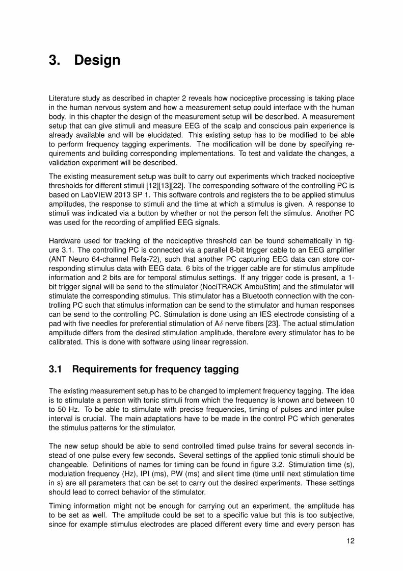
Hardware used for tracking of the nociceptive threshold can be found schematically in fig-ure 3.1. The controlling PC is connected via a parallel 8-bit trigger cable to an EEG amplifier(ANT Neuro 64-channel Refa-72), such that another PC capturing EEG data can store cor-responding stimulus data with EEG data. 6 bits of the trigger cable are for stimulus amplitudeinformation and 2 bits are for temporal stimulus settings. If any trigger code is present, a 1-bit trigger signal will be send to the stimulator (NociTRACK AmbuStim) and the stimulator willstimulate the corresponding stimulus. This stimulator has a Bluetooth connection with the con-trolling PC such that stimulus information can be send to the stimulator and human responsescan be send to the controlling PC. Stimulation is done using an IES electrode consisting of apad with five needles for preferential stimulation of Aδ nerve fibers [23]. The actual stimulationamplitude differs from the desired stimulation amplitude, therefore every stimulator has to becalibrated. This is done with software using linear regression.

3.1 Requirements for frequency tagging

The existing measurement setup has to be changed to implement frequency tagging. The ideais to stimulate a person with tonic stimuli from which the frequency is known and between 10to 50 Hz. To be able to stimulate with precise frequencies, timing of pulses and inter pulseinterval is crucial. The main adaptations have to be made in the control PC which generatesthe stimulus patterns for the stimulator.

The new setup should be able to send controlled timed pulse trains for several seconds in-stead of one pulse every few seconds. Several settings of the applied tonic stimuli should bechangeable. Definitions of names for timing can be found in figure 3.2. Stimulation time (s),modulation frequency (Hz), IPI (ms), PW (ms) and silent time (time until next stimulation timein s) are all parameters that can be set to carry out the desired experiments. These settingsshould lead to correct behavior of the stimulator.

Timing information might not be enough for carrying out an experiment, the amplitude hasto be set as well. The amplitude could be set to a specific value but this is too subjective,since for example stimulus electrodes are placed different every time and every person has

12

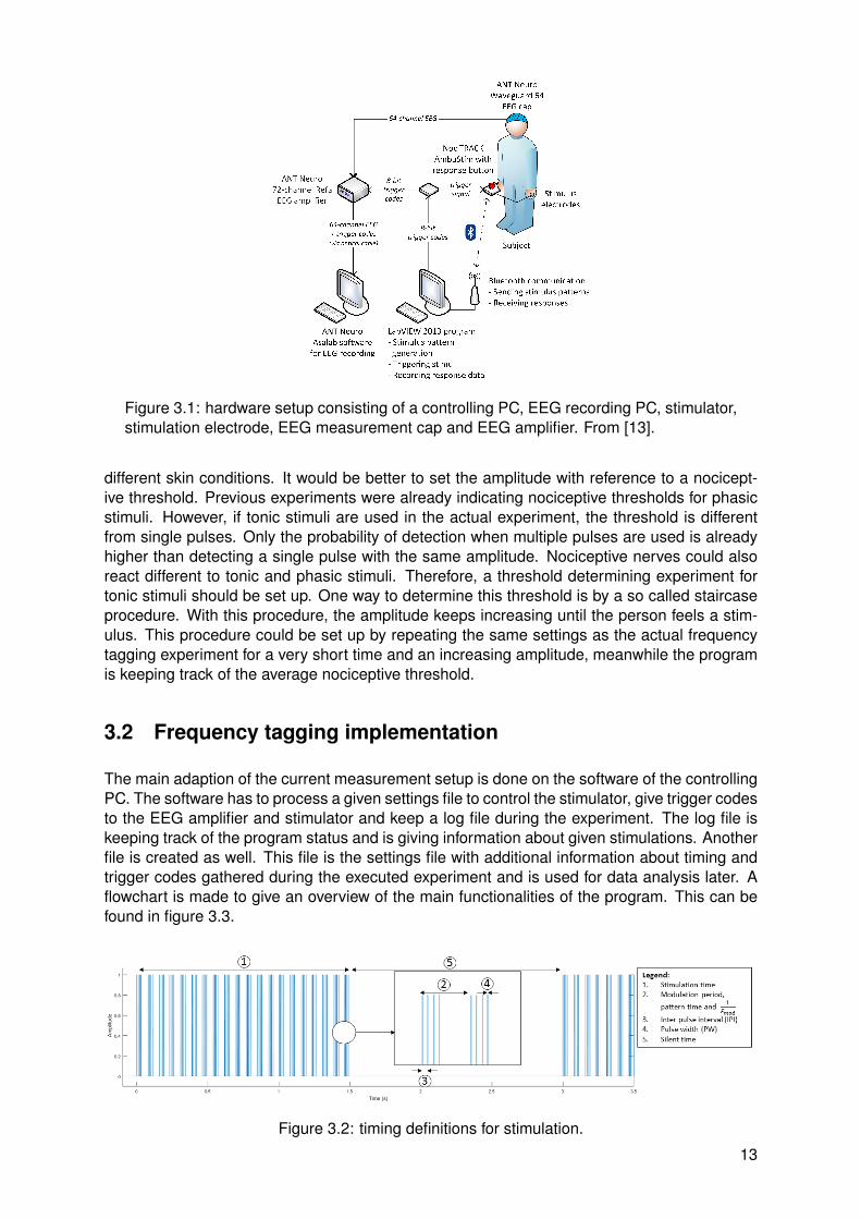
Figure 3.1: hardware setup consisting of a controlling PC, EEG recording PC, stimulator,stimulation electrode, EEG measurement cap and EEG amplifier. From [13].

different skin conditions. It would be better to set the amplitude with reference to a nocicept-ive threshold. Previous experiments were already indicating nociceptive thresholds for phasicstimuli. However, if tonic stimuli are used in the actual experiment, the threshold is differentfrom single pulses. Only the probability of detection when multiple pulses are used is alreadyhigher than detecting a single pulse with the same amplitude. Nociceptive nerves could alsoreact different to tonic and phasic stimuli. Therefore, a threshold determining experiment fortonic stimuli should be set up. One way to determine this threshold is by a so called staircaseprocedure. With this procedure, the amplitude keeps increasing until the person feels a stim-ulus. This procedure could be set up by repeating the same settings as the actual frequencytagging experiment for a very short time and an increasing amplitude, meanwhile the programis keeping track of the average nociceptive threshold.

3.2 Frequency tagging implementation

The main adaption of the current measurement setup is done on the software of the controllingPC. The software has to process a given settings file to control the stimulator, give trigger codesto the EEG amplifier and stimulator and keep a log file during the experiment. The log file iskeeping track of the program status and is giving information about given stimulations. Anotherfile is created as well. This file is the settings file with additional information about timing andtrigger codes gathered during the executed experiment and is used for data analysis later. Aflowchart is made to give an overview of the main functionalities of the program. This can befound in figure 3.3.

Figure 3.2: timing definitions for stimulation.

13

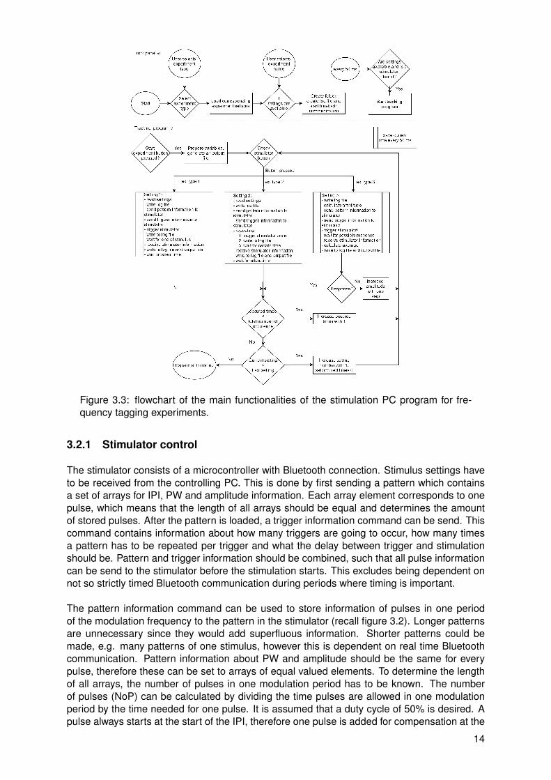
Figure 3.3: flowchart of the main functionalities of the stimulation PC program for fre-quency tagging experiments.

3.2.1 Stimulator control

The stimulator consists of a microcontroller with Bluetooth connection. Stimulus settings haveto be received from the controlling PC. This is done by first sending a pattern which containsa set of arrays for IPI, PW and amplitude information. Each array element corresponds to onepulse, which means that the length of all arrays should be equal and determines the amountof stored pulses. After the pattern is loaded, a trigger information command can be send. Thiscommand contains information about how many triggers are going to occur, how many timesa pattern has to be repeated per trigger and what the delay between trigger and stimulationshould be. Pattern and trigger information should be combined, such that all pulse informationcan be send to the stimulator before the stimulation starts. This excludes being dependent onnot so strictly timed Bluetooth communication during periods where timing is important.

The pattern information command can be used to store information of pulses in one periodof the modulation frequency to the pattern in the stimulator (recall figure 3.2). Longer patternsare unnecessary since they would add superfluous information. Shorter patterns could bemade, e.g. many patterns of one stimulus, however this is dependent on real time Bluetoothcommunication. Pattern information about PW and amplitude should be the same for everypulse, therefore these can be set to arrays of equal valued elements. To determine the lengthof all arrays, the number of pulses in one modulation period has to be known. The numberof pulses (NoP) can be calculated by dividing the time pulses are allowed in one modulationperiod by the time needed for one pulse. It is assumed that a duty cycle of 50% is desired. Apulse always starts at the start of the IPI, therefore one pulse is added for compensation at the

14

end of the duty cycle. The calculation for number of pulses can be found in equation 3.1. Here,the division is rounded down to the nearest integer, since it is only possible to have an integeramount of pulses. Because the result is always an integer, the duty cycle is slightly lower than50% in some cases. The inter pulse interval is different for different pulses in one period ofmodulation frequency. All pulses except the last one keep the initially specified IPI. The lastpulse is specified with a longer IPI to create a silent time in the last half of the modulationperiod. Calculation of the last IPI can be found in equation 3.2. Correction factors are addedat the calculation of IPI and NoP to go from seconds to milliseconds, since IPI is specified inmilliseconds.

NoP =

⌊1

2 ∗ Fmod ∗ IPI∗ 1000ms

⌋+ 1 (3.1)

IPIlast =1

Fmod∗ 1000ms− IPI ∗ (NoP − 1) (3.2)

The trigger information command is used in two ways. Delay is never used in both casesbecause accurate timing of trigger and stimulation is desired. First, the trigger command canbe specified to trigger once and repeat the pattern multiple times until the stimulation time isover. To calculate the total amount of patterns in one stimulation time equation 3.3 is used.Second, the trigger command can be specified to give multiple times a trigger and one patternper trigger. In this case the number of patterns in equation 3.3 should be replaced by numberof triggers.

No. Patterns = round( Stimulation timeModulation period

)= round(Stimulation time ∗ Fmod) (3.3)

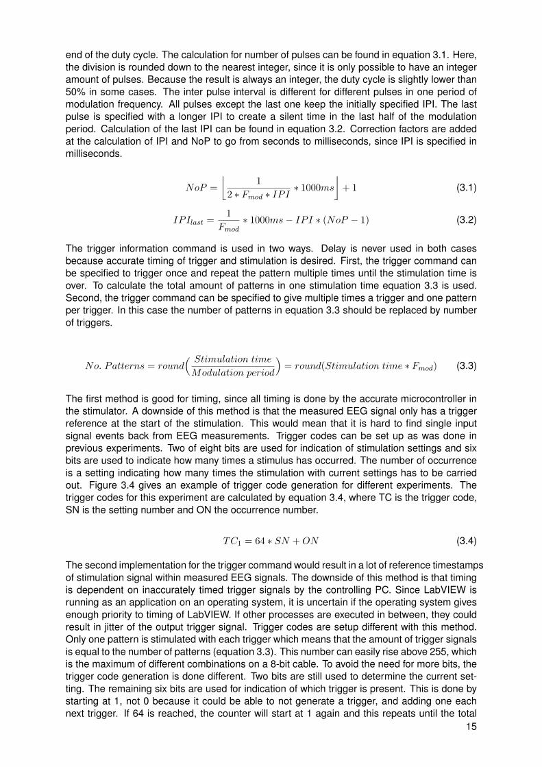
The first method is good for timing, since all timing is done by the accurate microcontroller inthe stimulator. A downside of this method is that the measured EEG signal only has a triggerreference at the start of the stimulation. This would mean that it is hard to find single inputsignal events back from EEG measurements. Trigger codes can be set up as was done inprevious experiments. Two of eight bits are used for indication of stimulation settings and sixbits are used to indicate how many times a stimulus has occurred. The number of occurrenceis a setting indicating how many times the stimulation with current settings has to be carriedout. Figure 3.4 gives an example of trigger code generation for different experiments. Thetrigger codes for this experiment are calculated by equation 3.4, where TC is the trigger code,SN is the setting number and ON the occurrence number.

TC1 = 64 ∗ SN +ON (3.4)

The second implementation for the trigger command would result in a lot of reference timestampsof stimulation signal within measured EEG signals. The downside of this method is that timingis dependent on inaccurately timed trigger signals by the controlling PC. Since LabVIEW isrunning as an application on an operating system, it is uncertain if the operating system givesenough priority to timing of LabVIEW. If other processes are executed in between, they couldresult in jitter of the output trigger signal. Trigger codes are setup different with this method.Only one pattern is stimulated with each trigger which means that the amount of trigger signalsis equal to the number of patterns (equation 3.3). This number can easily rise above 255, whichis the maximum of different combinations on a 8-bit cable. To avoid the need for more bits, thetrigger code generation is done different. Two bits are still used to determine the current set-ting. The remaining six bits are used for indication of which trigger is present. This is done bystarting at 1, not 0 because it could be able to not generate a trigger, and adding one eachnext trigger. If 64 is reached, the counter will start at 1 again and this repeats until the total

15

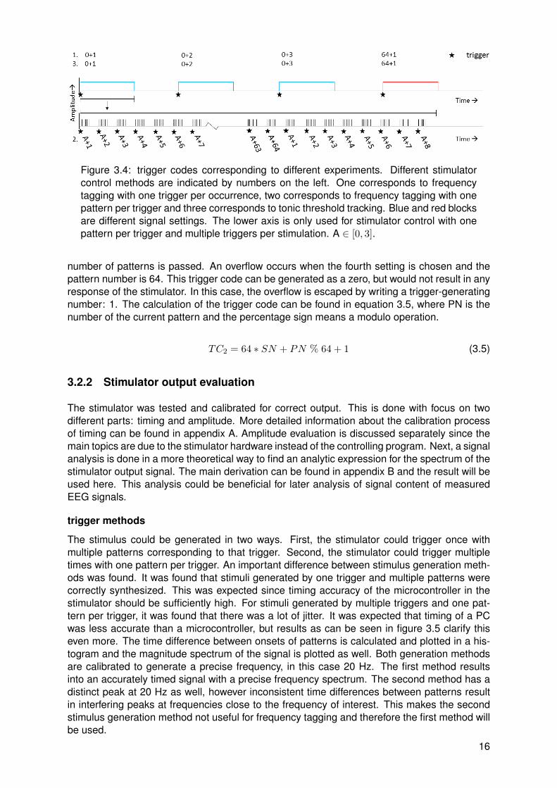
Figure 3.4: trigger codes corresponding to different experiments. Different stimulatorcontrol methods are indicated by numbers on the left. One corresponds to frequencytagging with one trigger per occurrence, two corresponds to frequency tagging with onepattern per trigger and three corresponds to tonic threshold tracking. Blue and red blocksare different signal settings. The lower axis is only used for stimulator control with onepattern per trigger and multiple triggers per stimulation. A ∈ [0, 3].

number of patterns is passed. An overflow occurs when the fourth setting is chosen and thepattern number is 64. This trigger code can be generated as a zero, but would not result in anyresponse of the stimulator. In this case, the overflow is escaped by writing a trigger-generatingnumber: 1. The calculation of the trigger code can be found in equation 3.5, where PN is thenumber of the current pattern and the percentage sign means a modulo operation.

TC2 = 64 ∗ SN + PN % 64 + 1 (3.5)

3.2.2 Stimulator output evaluation

The stimulator was tested and calibrated for correct output. This is done with focus on twodifferent parts: timing and amplitude. More detailed information about the calibration processof timing can be found in appendix A. Amplitude evaluation is discussed separately since themain topics are due to the stimulator hardware instead of the controlling program. Next, a signalanalysis is done in a more theoretical way to find an analytic expression for the spectrum of thestimulator output signal. The main derivation can be found in appendix B and the result will beused here. This analysis could be beneficial for later analysis of signal content of measuredEEG signals.

trigger methods

The stimulus could be generated in two ways. First, the stimulator could trigger once withmultiple patterns corresponding to that trigger. Second, the stimulator could trigger multipletimes with one pattern per trigger. An important difference between stimulus generation meth-ods was found. It was found that stimuli generated by one trigger and multiple patterns werecorrectly synthesized. This was expected since timing accuracy of the microcontroller in thestimulator should be sufficiently high. For stimuli generated by multiple triggers and one pat-tern per trigger, it was found that there was a lot of jitter. It was expected that timing of a PCwas less accurate than a microcontroller, but results as can be seen in figure 3.5 clarify thiseven more. The time difference between onsets of patterns is calculated and plotted in a his-togram and the magnitude spectrum of the signal is plotted as well. Both generation methodsare calibrated to generate a precise frequency, in this case 20 Hz. The first method resultsinto an accurately timed signal with a precise frequency spectrum. The second method has adistinct peak at 20 Hz as well, however inconsistent time differences between patterns resultin interfering peaks at frequencies close to the frequency of interest. This makes the secondstimulus generation method not useful for frequency tagging and therefore the first method willbe used.

16

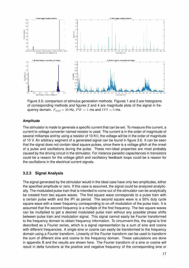
Figure 3.5: comparison of stimulus generation methods. Figures 1 and 3 are histogramsof corresponding methods and figures 2 and 4 are magnitude plots of the signal in fre-quency domain. Fmod = 20 Hz, PW = 1 ms and IPI = 5 ms.

Amplitude

The stimulator is made to generate a specific current that can be set. To measure this current, acurrent to voltage converter named resistor is used. The current is in the order of magnitude ofseveral milliamps and by using a resistor of 10 KΩ, the voltage will be in the order of magnitudeof 10 V. An arbitrary segment of a generated signal can be found in figure 3.6. It can be seenthat the signal does not contain ideal square pulses, since there is a voltage glitch at the onsetof a pulse and oscillations during the pulse. These non-ideal properties are most probablycaused by the driving circuit in the stimulator. For instance parasitic capacitances in transistorscould be a reason for the voltage glitch and oscillatory feedback loops could be a reason forthe oscillations in the electrical current signals.

3.2.3 Signal Analysis

The signal generated by the stimulator would in the ideal case have only two amplitudes, eitherthe specified amplitude or zero. If this case is assumed, the signal could be analyzed analytic-ally. The modulated pulse train that is intended to come out of the stimulator can be analyticallybe created from two square waves. The first square wave corresponds to a pulse train witha certain pulse width and the IPI as period. The second square wave is a 50% duty cyclesquare wave with a lower frequency corresponding to on-off modulation of the pulse train. It isassumed that the second frequency is a multiple of the first frequency. The two square wavescan be multiplied to get a desired modulated pulse train without any possible phase shiftsbetween pulse train and modulation signal. This signal cannot easily be Fourier transformedto the frequency domain to obtain frequency information. To circumvent this, the signal is firstdescribed as a Fourier series, which is a signal representation by a sum of sine and cosinewith different frequencies. A single sine or cosine can easily be transformed to the frequencydomain using a Fourier transform. Linearity of the Fourier transform can be used to transformthe sum of different sine and cosine to the frequency domain. These calculations are donein appendix B and the results are shown here. The Fourier transform of a sine or cosine willresult in delta functions at the positive and negative frequency of the corresponding sine or

17

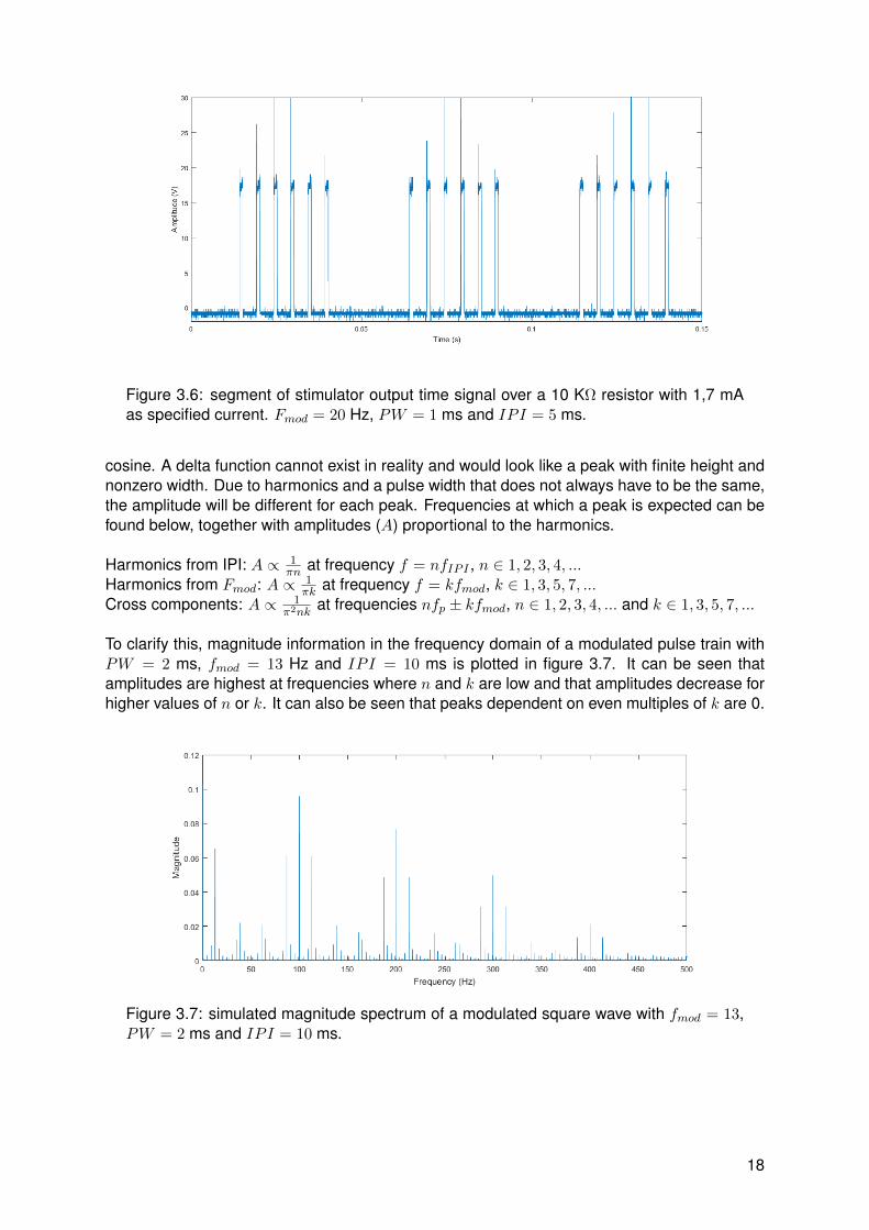
Figure 3.6: segment of stimulator output time signal over a 10 KΩ resistor with 1,7 mAas specified current. Fmod = 20 Hz, PW = 1 ms and IPI = 5 ms.

cosine. A delta function cannot exist in reality and would look like a peak with finite height andnonzero width. Due to harmonics and a pulse width that does not always have to be the same,the amplitude will be different for each peak. Frequencies at which a peak is expected can befound below, together with amplitudes (A) proportional to the harmonics.

Harmonics from IPI: A ∝ 1πn at frequency f = nfIPI , n ∈ 1, 2, 3, 4, ...

Harmonics from Fmod: A ∝ 1πk at frequency f = kfmod, k ∈ 1, 3, 5, 7, ...

Cross components: A ∝ 1π2nk

at frequencies nfp ± kfmod, n ∈ 1, 2, 3, 4, ... and k ∈ 1, 3, 5, 7, ...

To clarify this, magnitude information in the frequency domain of a modulated pulse train withPW = 2 ms, fmod = 13 Hz and IPI = 10 ms is plotted in figure 3.7. It can be seen thatamplitudes are highest at frequencies where n and k are low and that amplitudes decrease forhigher values of n or k. It can also be seen that peaks dependent on even multiples of k are 0.

Figure 3.7: simulated magnitude spectrum of a modulated square wave with fmod = 13,PW = 2 ms and IPI = 10 ms.

18

3.2.4 Threshold tracking

Threshold tracking is implemented to determine a reference for the stimulus amplitude in fre-quency tagging experiments. Threshold tracking of tonic stimuli is specifically added to thesetup. To determine the tonic nociceptive threshold, the amplitude of a pulse train stimulusis increased in steps until the stimulus is felt by the subject. The amplitude is determined byusing an increasing multiplier (m) multiplied by an amplitude resolution. An average thresholdis adapted with each response. A response is indicated by the human subject releasing thebutton on the stimulator. The pulse trains with different amplitudes are separated by a spe-cifiable silent time in which a reaction of the subject is received.

The different amplitudes are generated by one trigger per pulse train corresponding to oneamplitude. This is the same way as was done with frequency tagging and the one triggerand multiple patterns method. This is chosen to obtain high timing accuracy instead of manytime references for EEG, since the EEG responses of threshold tracking are not intended to beused. Different trigger codes are generated per different amplitude to be able to separate pulsetrains with different amplitudes in the log files. Two bits are reserved for different experimentsettings, the remaining bits are used to represent the amplitude. The value of the amplitudemultiplier will be used in the trigger code, as can be seen in equation 3.6. As a safety measure,the increasing amplitude cannot go beyond 2 mA.

TC3 = 64 ∗ SN +m (3.6)

19

4. Validation

A technical pilot study on one healthy human subject was performed to demonstrate and val-idate the new setup with implemented frequency tagging. Four different settings are used tostimulate the subject. First an average threshold of nociception was measured, which wasused tot determine the amplitude for actual frequency tagging. The cortical activities duringfrequency tagging stimulation are measured with EEG. The EEG signals of electrode deriva-tions C4-Fpz, C3-Fpz and Cz-M1M2 will be analyzed to investigate potential relations betweencortical activities and stimuli.

4.1 Materials and methods

4.1.1 Human subject

One participant (male, aged 21 years, right handed) took part in the experiment. The parti-cipant was healthy and pain-free. The participant did not consume any energizers or tranquil-izers (e.g. coffee or alcohol) from 24 hours before the experiment and onwards. The parti-cipant slept well the night before the experiment and had a good breakfast. The participantwas informed by an information letter which can be found in appendix C. The experimentalprocedures were approved by the local ethics committee.

4.1.2 Stimuli

The subject was stimulated with modulated pulse trains. Cathodic square wave controlledcurrent pulses of 1 ms PW, separated by 10 ms IPI, were used. The pulse train was modulatedon and off with frequencies 13, 20, 33 and 43 Hz. These frequencies were chosen to measurea wide frequency band as well as prevent possible harmonics between different modulationfrequencies. The stimulus amplitude was set to twice the perceptual threshold, estimated byan increasing staircase procedure of a similar modulated pulse train with a duration of 2s peramplitude to generate a definite pain sensation. IES stimulation was used to preferentiallyactivate Aδ-fibers on the back of the left hand. The electrode consisted of five needles, basedon a bimodal design [23]. A TENS electrode was used as anode and was placed on the lowerarm. The electrodes were connected to the setup as described in chapter 3.

4.1.3 Procedure

Experiments were executed in a lighted, silent and temperature-controlled room. The subjectsat in a comfortable armchair. The electrodes for stimulation were applied to the subject and asmall test was done. This was to check for correct functioning of the stimulation and to comfortthe subject. The EEG cap was then applied, where after the nociceptive threshold was determ-ined. EEG was not recorded during the threshold tracking and the time needed for thresholdtracking served for settling of impedances in the cap on the head as well. The amplitude wasincreased until the subject felt a stimulation. At that moment the subject was instructed to re-lease the button of the stimulator. This was repeated 10 times for each modulating frequencyand the average threshold per frequency was taken. After the nociceptive threshold was ap-proximated, the pulse train amplitude was set to double this value. Each pulse train was set toa duration of 10 s and a 10 s silent time afterwards. The subject was able to take a break or

20

to drink cold water between any of the stimuli by releasing the button on the stimulator. Thesubject was asked to blink as few as possible, concentrate and focus on a fixed point duringthe stimuli. Pulse trains with different frequency were each repeated 10 times. The total timein which stimulations were applied was approximately 30 minutes.

4.1.4 EEG measures

EEG signals were recorded using an EEG cap (ANT Neuro Waveguard) placed on the scalp.The cap contained 64 Ag/AgCl electrodes. Signals coming from the electrodes were amplifiedusing an ANT Neuro 64-channel Refa-72 EEG amplifier and saved together with stimulus trig-ger codes on a PC. All channels were sampled with 1 kHz. All electrode impedances on thecap were kept below 5 kΩ and the ground electrode was placed on the forehead.

4.1.5 Data analysis

The trigger and EEG information was analyzed using Matlab and an EEG/MEG analysis tool-box called FieldTrip. Non-overlapping EEG segments were obtained by partitioning the EEGrecording relative to ten seconds before and ten seconds after all trigger times. All EEG seg-ments were filtered using a fifth order 2-480 Hz bandpass filter for removal of frequencies notrelevant for this experiment and anti aliasing. Fifth order bandstop filters with center frequen-cies 50, 150, 250 and 350 Hz were used on all segments as well to remove components fromthe electrical grid. Eye blinking artifacts were not removed from any trials.

For each EEG segment, channel derivations C4-Fpz, C3-Fpz and Cz-M1M2 were derived.The first two channel derivations were chosen to take a bigger dipole moment into accountrelative to C4-Fz and C3-Fz in literature. Segments were processed in two ways per setting.First, the average of all individual segments was taken and the result was transformed usinga wavelet transform. This sequence corresponds to a phase locked analysis. The wavelettransform will be tapered based on multiplication in the frequency domain and relative baselinecorrection is used for plotting. Second, the time during stimulus in each segment is processed.This was done by first averaging the time signals and subsequently applying a FFT transform(phase locked analysis) and by first FFT transforming each individual signal and subsequentlyaveraging the magnitude spectrum (non phase locked analysis). Averaged signals in the fre-quency domain obtained via both methods are subsequently averaged relative to neighboringfrequencies. The average of each frequency in ±1 Hz around the center frequency was sub-tracted for each possible frequency in the spectrum.

To obtain more information about the signal around the stimulus onset, separate analysis wasdone 50 ms around the trigger. Phase locked and non phase locked FFT analysis across allsegment with the same modulation frequency was done separate and the signals from -50 to 0and from 0 to +50 ms relative to the trigger were separated as well. Motivation for this is the lim-ited conduction velocity of the stimulus signal in the nervous system. C-, Aδ- and Aβ-fibers allhave different conduction velocities (respectively 1-4, 10-15 and 50-70 m/s [24]). These velo-cities already imply that C- and Aδ-fibers have a too slow conduction speed to arrive at corticesin a time less than 50 ms if a distance of 0.5-1 m in the periphery is assumed. On top of this,measurements of responses to nociceptive (Aδ-fiber) stimuli show first responses around 202ms after stimulus onset and stimulation with non nociceptive (Aβ-fiber) stimuli show that firstresponses of the former are around 134 ms [25]. This indicates that the non nociceptive pathhas a higher velocity, but still arrives later than 50 ms in cortices. These measurements verifythat time from stimulus onset to 50 ms afterwards does not contain cortical responses yet.If components of the input signal would be measured here, this would indicate that stimulusartifacts are measured in EEG signals.

21

4.2 Results

Results of frequency tagging with different modulation frequencies, 13, 20, 33 and 43 Hz, canrespectively be found in figures 4.1, 4.2, 4.3 and 4.4. Different plots are made: one for thetime signals around stimulus onset, time-frequency plots for a global overview of all data intime and frequency domain and magnitude spectrum plots in the frequency domain to have aclearer view of frequency content during stimulation. Channel derivations C4-Fpz, C3-Fpz andCz-M1M2 are analyzed separate and are represented per column. All measurement data wasbased on 10 trials.

From the time signal plots around stimulus onset it can be seen that for the channel derivationsC4-Fpz and C3-Fpz there are differences between before and after stimulus onset. After stim-ulus onset, it seems that there are strange components in the EEG signal, which seem similarto the stimulus pulse train. From the time plot of channel Cz-M1M2 for all different modulationfrequencies, it can be seen that a phasic response is present after stimulus onset. This maybe an event related potential called P300, corresponding to cognitive processing.

From the time frequency plots, it can be seen which frequencies are present at which time.For all different modulation frequencies, it can be seen that distinctive frequencies correspond-ing to multiples of the modulation frequency, multiples of the frequency corresponding to theIPI of 10 ms and combinations of both multiples are present. The magnitude of these fre-quencies seems to be less in channel derivation Cz-M1M2. For segments corresponding tomeasurements of a modulation frequency of 20 Hz, it can be seen that there is much activity atfrequencies spread around the spectrum. This is most probably due to noise from eye blinkingartifacts in the recordings.

In the third row of figures with data, the magnitude with subtracted relative average can beseen. This is analyzed in both phase locked and non phase locked methods. Considering alldata from all modulation frequencies, it can be said that peaks occur at combinations of mul-tiples of the modulation frequency or multiples of the frequency corresponding to 10 ms IPI.These are frequencies that can be derived from the frequencies present in the input signal asanalyzed in section 3.2.2. Proportionality of peak amplitude seems to coincide with expecta-tions most of the times. At each peak, both phase locked and non phase locked componentsare present and in most cases the non phase locked components have higher magnitude. Thismeans that responses cannot be categorized as one of the two types.

For the modulation frequency of 13 Hz, it can be seen that distinct peaks are not presentunder 87 Hz. If the higher frequencies are considered, the highest peaks occur at the frequen-cies corresponding to the IPI. Frequency peaks at a distance of multiples of 13 hz from thiscan be found back in the whole spectrum. At the higher half of frequencies, multiple peaks withrelatively low amplitudes are found. These correspond to combinations of higher harmonics ofthe modulation frequency and frequencies corresponding to the IPI.

If pulses modulated with 20 Hz are considered, it can be seen that most of the spectral peaksare again at the higher frequencies. In this case, peaks at 80 Hz and higher are distinct. Ifthe spectrum of channel derivation C4-Fpz is looked more closely, a small peak is present at20 Hz. If the spectrum of channel derivation C3-Fpz is looked more closely, peaks at 20, 40and 60 Hz are present. These peaks are barely distinct, but still specific at a multiple of themodulation frequency.

Specific for the modulation frequency 33 Hz is that all lower harmonics 33, 67, 99, 100 Hz,etc. are found back in the EEG signal of channel derivations C4-Fpz and C3-Fpz. This doesnot appear as clearly in Cz-M1M2. For these low frequencies, the ratio of phase locked and

22

non phase locked is relatively high. As frequency increases, this ratio decreases.

Results corresponding to a modulation frequency of 43 Hz seem to be quite similar to resultsof 33 Hz. Channel derivations C4-Fpz and C3-Fpz show harmonics with a higher amplitudethan Cz-M1M2, revealing less powerful frequencies as well. Notable is that multiples of thefrequency corresponding to the IPI are not present at precisely 100, 200 and 400 Hz, but atfrequencies which are a multiple of the modulation frequency close by.

It is quite strange that high frequencies (>150 Hz) are present in EEG signals. It could bethat peaks in this range correspond to stimulus artifacts. This is inspected by looking at thesignal of all trials 50 ms before and after the stimulus onset. Signals going from the hand tothe brain via the nervous system should take a time larger than 50 ms to travel as discussed inthe methods. Results corresponding to all stimulations with 33 Hz modulation frequency canbe found in figure 4.5. The plots are zero padded with a length of 150 samples to gain morefrequency accuracy. Plots of 50 ms before and after stimulus onset of all modulation frequen-cies can be found in appendix D. Only one plot is shown here, since all plots show the same.Peaks centered at multiples of 100 Hz (corresponding to 10 ms IPI) on channel derivationsC4-Fpz and C3-Fpz are visible with a clear amplitude in time after the stimulus. Specific peakscannot be found in the spectrum corresponding to time before the stimulus onset. Channelderivation Cz-M1M2 shows peaks at multiples of 100 Hz as well, only with a relatively loweramplitude.

23

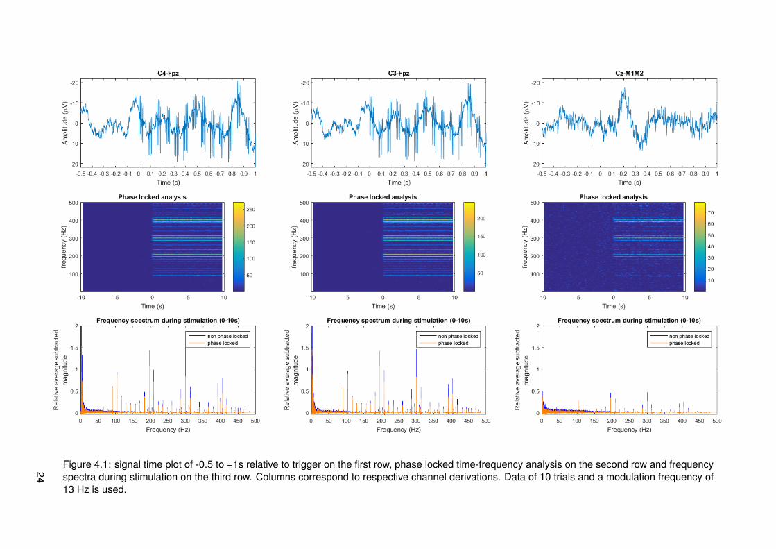
Figure 4.1: signal time plot of -0.5 to +1s relative to trigger on the first row, phase locked time-frequency analysis on the second row and frequencyspectra during stimulation on the third row. Columns correspond to respective channel derivations. Data of 10 trials and a modulation frequency of13 Hz is used.

24

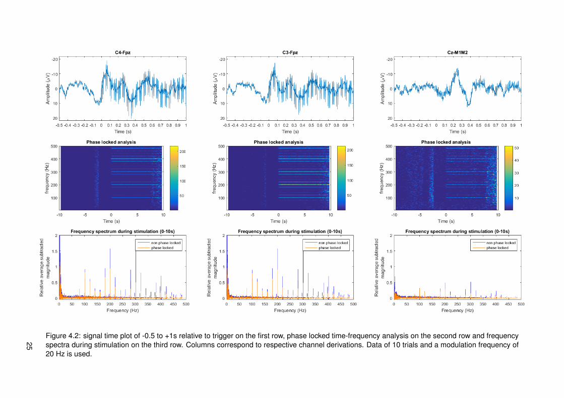
Figure 4.2: signal time plot of -0.5 to +1s relative to trigger on the first row, phase locked time-frequency analysis on the second row and frequencyspectra during stimulation on the third row. Columns correspond to respective channel derivations. Data of 10 trials and a modulation frequency of20 Hz is used.

25

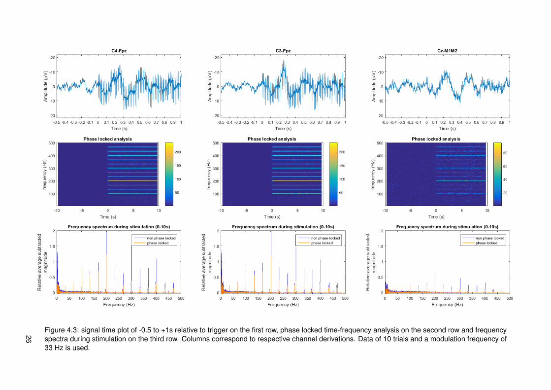
Figure 4.3: signal time plot of -0.5 to +1s relative to trigger on the first row, phase locked time-frequency analysis on the second row and frequencyspectra during stimulation on the third row. Columns correspond to respective channel derivations. Data of 10 trials and a modulation frequency of33 Hz is used.

26

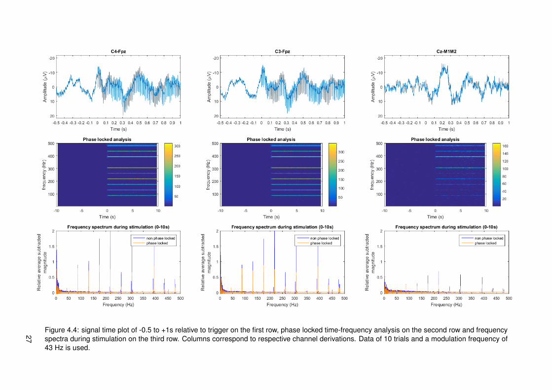
Figure 4.4: signal time plot of -0.5 to +1s relative to trigger on the first row, phase locked time-frequency analysis on the second row and frequencyspectra during stimulation on the third row. Columns correspond to respective channel derivations. Data of 10 trials and a modulation frequency of43 Hz is used.

27

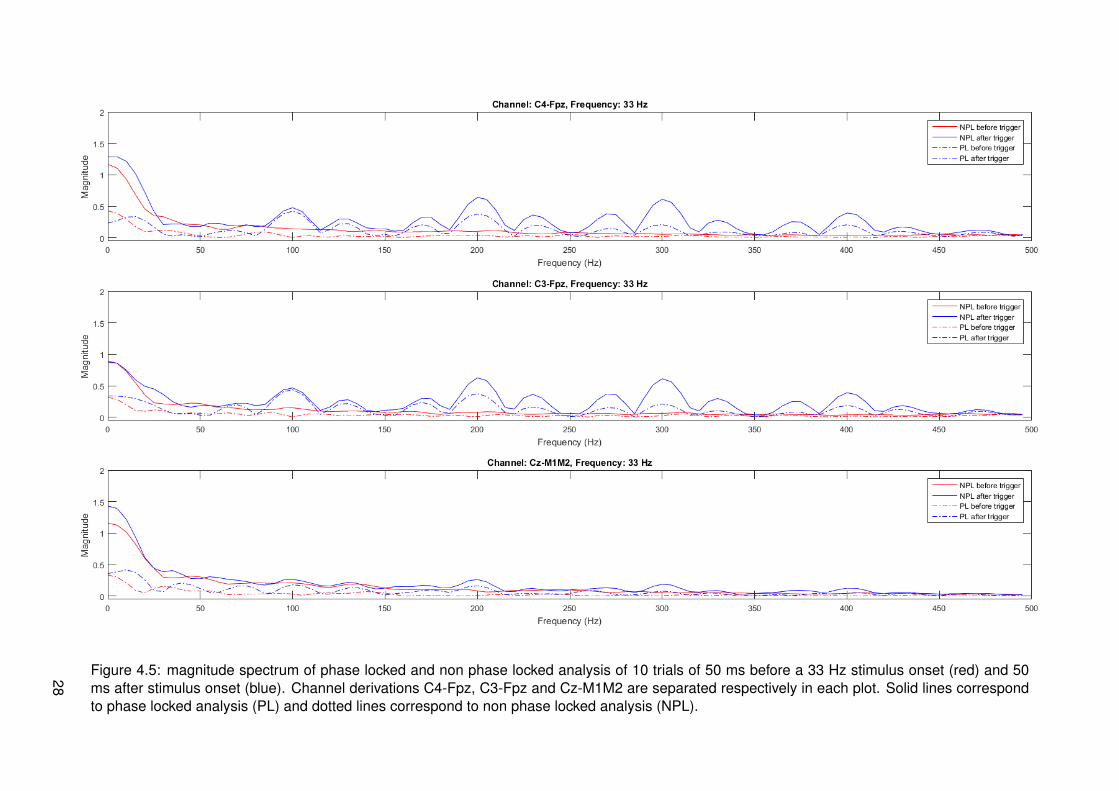
Figure 4.5: magnitude spectrum of phase locked and non phase locked analysis of 10 trials of 50 ms before a 33 Hz stimulus onset (red) and 50ms after stimulus onset (blue). Channel derivations C4-Fpz, C3-Fpz and Cz-M1M2 are separated respectively in each plot. Solid lines correspondto phase locked analysis (PL) and dotted lines correspond to non phase locked analysis (NPL).

28

5. Discussion

Outcome of this research can be interpreted in many different ways. An example is alreadypresent in the many different representation of EEG measurements in the validation experi-ment. Since these EEG recordings give the result of an experiment, this experiment can beevaluated. The implemented setup to execute this experiment can thereby very well be evalu-ated to its functional extend according to the experiment results.

5.1 Experiment

An experiment was done on a human subject in which electrical current pulses stimulated theleft hand to consecutively measure EEG signals from the scalp. Stimulation was done via apulse train that was modulated on and off with a certain frequency. EEG data from channelderivations C4-Fpz, C3-Fpz and Cz-M1M2 was analyzed.

The experiment was conducted on only one human subject. This leads to very biased results.This bias could be large, such that data that is interpreted from these measurements couldlead to different conclusions than measurement data based on measurements of another hu-man subject or combinations of human subjects. Another factor making the measurementsbiased is the presence of eye blinking artifacts. Only 10 trials are considered, if one trial wouldconsist of an eye blinking artifact, the time average data is already affected significantly for aspecific time.

Measurement results show that difference of EEG signals during stimuli and before stimuliare clearly visible. Signal content during the stimuli contains multiple sharp peaks at specificfrequencies. The steepness of these peaks is already an indication of precisely timed stim-ulation. The frequencies at which the peaks occur are related to the stimulus signal. Peaksoccur at frequencies that are a multiple or a linear combination of either the frequency at whichthe signal is modulated or the frequency which corresponds to timing of single pulses. Bycomparing calculations of the frequency content of the input signal and frequency content ofthe EEG measurements, peaks seem to occur at frequencies that coincide. Expected peakfrequencies below approximately 75 Hz are only clearly found back in measurements with amodulation frequency of 33 Hz. It is strange that EEG measurements do almost not show lowfrequencies and do show frequency content with high amplitude on higher frequencies. Thiscould be an indication that signals are conducted via a different route than the nervous sys-tem. Such a different route would imply that the peaks at higher frequencies in the spectrumare caused by stimulus artifacts. Further investigation verifies this by showing that frequencycontent corresponding to the input signal is present in EEG recordings from stimulus onset to50 ms afterwards. If stimulus artifacts are assumed to be present in EEG recordings, it cannotbe said which part of the frequency content is actual measured cortical activity or is due tostimulus artifacts. To do further investigation on stimulus artifacts, the cause has to be found.Stimulus artifacts in EEG recordings could be investigated by measuring the output signal ofthe stimulator or by analyzing conductive pathways in the human body, combinations of thesecauses could be modeled to gain more knowledge.

29

5.2 Measurement setup

A measurement setup was improved to be able to do nociceptive frequency tagging experi-ments. Main requirements of this improvement were ability to generate precisely timed pulsesand a variable controlled amplitude. During calibration and tests on a human subject it wasfound that precise timing can be achieved by the setup. Different ways of controlling stimulatoroutput were tested. Timing can be done correctly if it is completely managed by the micro-controller in the stimulator. A lot of jitter in timing was found when managed by a programcontrolling a parallel port on a desktop pc. This inaccurate timing resulted in noise and incor-rect frequency peaks in the magnitude spectrum of the signal.

Not much emphasis was placed on the amplitude of the signal generated by the stimulator.The signal showed a high voltage glitch at the onset of a pulse and oscillation during the pulse.This was implicitly assumed to not be problematic for the experiment. After observing stimulusartifacts in EEG recordings, the high voltage glitch is thought to be an origin for this. Oscilla-tions in the amplitude height could lead to inaccuracy if a very precise amplitude is desired. Inthis experiment this was not the case. The non-ideal properties of stimulation signal amplitudecould be caused by internal circuits of the stimulator. Thus to solve non-ideal properties, thiscircuit needs to be improved.

30

6. Conclusion

The conclusion of this bachelor assignment is split up into two parts. First, conclusions aboutthis work are drawn and second, recommendations for future research are given.

6.1 Conclusions

Increasing insight into nociceptive neural processing would lead to better understanding andtreatment of increased pain sensitivity. An observation method to gain new insights is fre-quency tagging. This method uses tonic stimuli with a controlled frequency content to observecorresponding nociceptive cortical information. An implementation of a setup that can be usedfor frequency tagging experiments was made. Results show that tonic stimuli with precise fre-quency content can be generated. Experiments with one human subject show that frequenciesas a response to the input signal can be found back in EEG recordings. However, the exper-iments reveal that frequency content is available in EEG recordings in time after the stimulusonset and before cortical responses are possible. This is an indication of stimulus artifactsthat are present in the EEG recordings, making measurements not interpretable for analysisof neural processing. If issues with stimulus artifacts in EEG recordings would be solved, thissetup could be considered ready for frequency tagging experiments.

6.2 Recommendations

If future research is followed up on this work, the following recommendations might be takeninto account:

• Two different methods were used to generate timed stimuli. The stimulator was set togenerate multiple patterns if one trigger was present or the stimulator was set to gen-erate one pattern per trigger with multiple trigger signals. These two methods are com-pletely opposite to each other. A compromise could be made where multiple patternsare generated per trigger and multiple triggers are given per stimulation. This results ina tradeoff between timing accuracy and time references, since more patterns per triggerresults in more timing accuracy and more triggers result in more time references in EEGrecordings.

• The stimulator is programmed to accept patterns up to a certain length. If low modulationfrequencies are desired, this value might have to be increased to let the stimulator workcorrectly.

• The validation experiment was conducted on only one human subject. To verify that ameasurement setup is valid, it would be better to test on multiple human subjects. Astatistical analysis could be an aid for determining the necessary amount of subjects.

• Stimulus pulse trains were modulated with a certain frequency. If responses from multiplefrequencies are desired, the process of doing so could be facilitated by modulating thepulse trains with multiple frequencies at the same time instead of stimulating with differentfrequencies separated.

• A smart choice of stimulus parameters is required. Frequency magnitude spectra ofEEG recordings show that peaks occur at certain frequencies. The specific paramet-ers determining the frequency at which the peaks occur (IPI, Fmod) should have least

31

possible multiples that are the same to prevent occurrence of harmonics at the samefrequency corresponding to both parameters. This keeps cause and effect separatedbetween parameters.

• The frequency of the electrical grid (50 Hz) and corresponding odd harmonics can befound back in EEG recordings. Frequencies corresponding to chosen parameters shouldnot coincide with these frequencies to keep a single cause for each frequency peak andto be able to apply band stop filters for frequencies corresponding to the grid withoutlosing relevant measurement data.

• To track the cause of stimulus artifacts in EEG recordings, several different approachescould be useful. The circuit generating the stimulus in the stimulator could be analyzedand improved such that voltage glitches and oscillations are reduced. It is not certain thatstimulus artifacts in EEG recordings are caused by the stimulator. A study researchingnot only pathways in the nervous system but also in other possible conductive path-ways between stimulus location and cortices could be done. Non-ideal stimuli from thestimulator could be modeled in this study to gain knowledge on corresponding signalprocessing.

• The amplitude of stimulation pulses was determined using nociceptive threshold trackingby a staircase procedure. This method could not be accurate enough. Therefore, differenttypes of threshold tracking experiments could be done. Another option could be to letthe human subject give a rating of the stimulus intensity. This rating could be usedas feedback for the chosen amplitude and reflection of measured magnitude in EEGrecordings.

32

7. Acknowledgments

I would like to thank my supervisor Jan Buitenweg for his guidance during this bachelor as-signment. Hints to undertake certain steps during the assignment triggered my mind to thinkin other ways which resulted to be very useful. I would also like to thank the subject for his par-ticipation during the experiments. I would like my parents, brother and sister for their supportand believing in me.

33

References

[1] Dale Purves, George J. Augustine and David Fitzpatrick. Neuroscience. 2004. ISBN:0878937250.

[2] Charles R Noback et al. The Human Nervous System, Structure and Function. 2005.ISBN: 1588290395.

[3] M.N. Baliki, P.Y. Geha and A.V. Apkarian. “Parsing pain perception between nociceptiverepresentation and magnitude estimation”. In: Journal of Neurophysiology 2 (2009).

[4] A.V. Apkarian et al. “Human brain mechanisms of pain perception and regulation inhealth and disease”. In: European Journal of Pain 4 (2005).

[5] M.J. Millan. “Descending control of pain”. In: Progress in Neurobiology 6 (2002).[6] Irene Tracey. “Nociceptive processing in the human brain”. In: Current Opinion in Neuro-

biology 4 (2005).[7] A. Mouraux, G. D. Iannetti and L. Plaghki. “Low intensity intra-epidermal electrical stim-

ulation can activate Aδ-nociceptors selectively”. In: Pain 150.1 (2010).[8] L. Plaghki and A. Mouraux. “How do we selectively activate skin nociceptors with a high

power infrared laser? Physiology and biophysics of laser stimulation”. In: Neurophysiolo-gie Clinique 6 (2003).

[9] B. Bromm and R.D. Treede. “Nerve fibre discharges, cerebral potentials and sensationsinduced by CO2 laser stimulation”. In: Human Neurobiology 1 (1984).

[10] A. Mouraux, E. Marot and V. Legrain. “Short trains of intra-epidermal electrical stimulationto elicit reliable behavioral and electrophysiological responses to the selective activationof nociceptors in humans”. In: Neuroscience Letters (2014).

[11] Esther M van der Heide et al. “Single pulse and pulse train modulation of cutaneouselectrical stimulation: a comparison of methods.” In: Journal of clinical neurophysiology :official publication of the American Electroencephalographic Society 1 (2009).

[12] Robert J. Doll et al. “Effect of temporal stimulus properties on the nociceptive detectionprobability using intra-epidermal electrical stimulation”. In: Experimental Brain Research1 (2015).

[13] Marc Schooneman. “Measurement of evoked potentials during multiple threshold track-ing of nociceptive electrocutaneous stimuli”. In: ().

[14] Nihan Alp et al. “Frequency tagging yields an objective neural signature of Gestalt form-ation”. In: Brain and Cognition (2016).

[15] E. Colon, V. Legrain and A. Mouraux. “EEG frequency tagging to dissociate the corticalresponses to nociceptive and nonnociceptive stimuli”. In: Journal of cognitive neuros-cience 10 (2014).

[16] Athanasia Moungou, Jean-Louis Thonnard and Andre Mouraux. “EEG frequency taggingto explore the cortical activity related to the tactile exploration of natural textures”. In:Scientific Reports (2016).

[17] Elisabeth Colon et al. “Steady-state evoked potentials to tag specific components ofnociceptive cortical processing”. In: NeuroImage 1 (2012).

[18] Alexey M Ivanitsky et al. “Electroencephalography”. In: Encyclopedia of Neuroscience(2009).

[19] David Cohen and B. Neil Cuffin. “Demonstration of useful differences between magne-toencephalogram and electroencephalogram”. In: Electroencephalography and ClinicalNeurophysiology 1 (1983).

[20] Z. G. Zhang et al. “Gamma-Band Oscillations in the Primary Somatosensory Cortex - ADirect and Obligatory Correlate of Subjective Pain Intensity”. In: Journal of Neuroscience22 (2012).

34

[21] Aapo Hyvarinen and Erkki Oja. “Independent Component Analysis: Algorithms and Ap-plications”. In: Analysis 1 (2004).

[22] Robert J Doll et al. “Tracking of nociceptive thresholds using adaptive psychophysicalmethods.” In: Behavior Research Methods 1 (2014).

[23] P. Steenbergen et al. “Characterization of a bimodal electrocutaneous stimulation device”.In: IFMBE Proceedings (2008).

[24] Ryusuke Kakigi et al. “Cerebral responses following stimulation of unmyelinated C-fibersin humans: Electro- and magneto-encephalographic study”. In: Neuroscience Research3 (2003).

[25] K. Inui et al. “A comparative magnetoencephalographic study of cortical activations evokedby noxious and innocuous somatosensory stimulations”. In: Neuroscience 1 (2003).

35

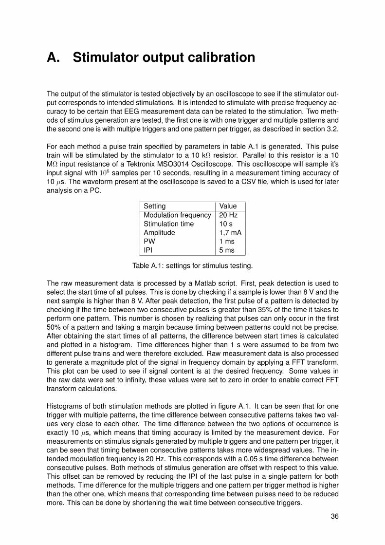
A. Stimulator output calibration

The output of the stimulator is tested objectively by an oscilloscope to see if the stimulator out-put corresponds to intended stimulations. It is intended to stimulate with precise frequency ac-curacy to be certain that EEG measurement data can be related to the stimulation. Two meth-ods of stimulus generation are tested, the first one is with one trigger and multiple patterns andthe second one is with multiple triggers and one pattern per trigger, as described in section 3.2.

For each method a pulse train specified by parameters in table A.1 is generated. This pulsetrain will be stimulated by the stimulator to a 10 kΩ resistor. Parallel to this resistor is a 10MΩ input resistance of a Tektronix MSO3014 Oscilloscope. This oscilloscope will sample it’sinput signal with 106 samples per 10 seconds, resulting in a measurement timing accuracy of10 µs. The waveform present at the oscilloscope is saved to a CSV file, which is used for lateranalysis on a PC.

Setting ValueModulation frequency 20 HzStimulation time 10 sAmplitude 1,7 mAPW 1 msIPI 5 ms

Table A.1: settings for stimulus testing.

The raw measurement data is processed by a Matlab script. First, peak detection is used toselect the start time of all pulses. This is done by checking if a sample is lower than 8 V and thenext sample is higher than 8 V. After peak detection, the first pulse of a pattern is detected bychecking if the time between two consecutive pulses is greater than 35% of the time it takes toperform one pattern. This number is chosen by realizing that pulses can only occur in the first50% of a pattern and taking a margin because timing between patterns could not be precise.After obtaining the start times of all patterns, the difference between start times is calculatedand plotted in a histogram. Time differences higher than 1 s were assumed to be from twodifferent pulse trains and were therefore excluded. Raw measurement data is also processedto generate a magnitude plot of the signal in frequency domain by applying a FFT transform.This plot can be used to see if signal content is at the desired frequency. Some values inthe raw data were set to infinity, these values were set to zero in order to enable correct FFTtransform calculations.

Histograms of both stimulation methods are plotted in figure A.1. It can be seen that for onetrigger with multiple patterns, the time difference between consecutive patterns takes two val-ues very close to each other. The time difference between the two options of occurrence isexactly 10 µs, which means that timing accuracy is limited by the measurement device. Formeasurements on stimulus signals generated by multiple triggers and one pattern per trigger, itcan be seen that timing between consecutive patterns takes more widespread values. The in-tended modulation frequency is 20 Hz. This corresponds with a 0.05 s time difference betweenconsecutive pulses. Both methods of stimulus generation are offset with respect to this value.This offset can be removed by reducing the IPI of the last pulse in a single pattern for bothmethods. Time difference for the multiple triggers and one pattern per trigger method is higherthan the other one, which means that corresponding time between pulses need to be reducedmore. This can be done by shortening the wait time between consecutive triggers.

36

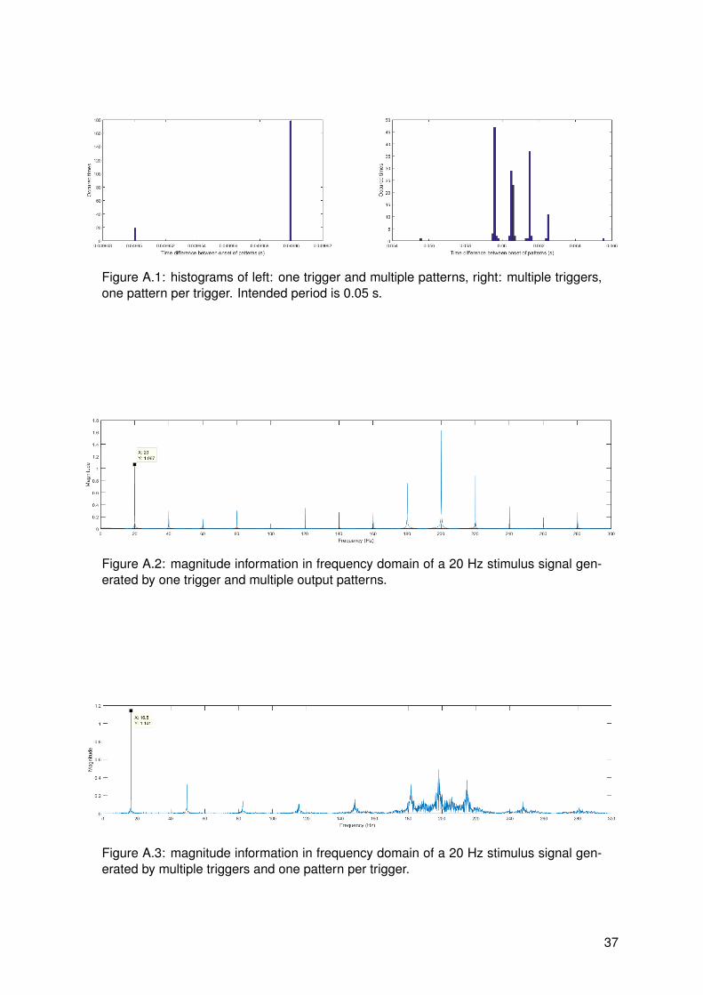
Figure A.1: histograms of left: one trigger and multiple patterns, right: multiple triggers,one pattern per trigger. Intended period is 0.05 s.

Figure A.2: magnitude information in frequency domain of a 20 Hz stimulus signal gen-erated by one trigger and multiple output patterns.

Figure A.3: magnitude information in frequency domain of a 20 Hz stimulus signal gen-erated by multiple triggers and one pattern per trigger.

37

Figure A.2 and A.3 show the magnitude plot in frequency domain of the different stimulus gen-eration methods. It can be seen that the most important peak, around 20 Hz, is not at 20 Hzin figure A.3. This is due to the offset that was already observed from the histograms. In figureA.2 a very strong component around 200 Hz is present. This corresponds to the frequencyrepresentation of single pulses of 5 ms IPI. In figure A.3 it can be seen that 200 Hz peak is nota distinct peak but a frequency band with a lot of noisy amplitudes. It is assumed that this isa consequence of the widespread timing variations between consecutive patterns, also knownas jitter. Apparently this jitter has more effect on higher than on lower frequencies, since thepeak at 16.5 Hz is still very distinct.

To improve the timing performance of both methods, timing offsets have to be removed. Offsetcan be removed by reducing the IPI of the last pulse in a pattern, however the signals gener-ated by one trigger and multiple patterns are at the right frequency so this is not needed. Themethod of multiple triggers and one pattern per trigger needs further improvement which willbe done by reducing the wait time between triggers. Figure A.3 shows a clear peak at 16.5Hz. This corresponds with a period of 60.606 ms. To change the frequency of multiple triggersand one pattern per trigger to 20 Hz, the wait time between triggers has to be reduced with:60.606− 50 = 10.606 ms. Labview only supports timing with an accuracy of milliseconds, so 11ms will be used.

To see if removing timing offsets helps, the calculated offset was subtracted from the wait-ing time. Another measurement with the same settings as before, mentioned in table A.1, wasexecuted. Results can be found in the histogram in figure A.4 and in the magnitude plot in fig-ure A.5. From figure A.4 it can be seen that the time differences between pattern onset are stillquite different values, one value is quite close to the intended period of 0.05 s. The second oneis present at double the intended frequency. From figure A.5 it can be seen that the intendedfrequency is represented by a sharp peak. This is good, however high peaks occur in neigh-boring frequencies as well, which are a result of periodic repetition of periodic unequal waitingtimes between onset of patterns. It was found that performance was not improved by choosingother constants to change waiting time of pattern generation. Two Labview functions were triedas different implementation, but both ’wait (ms)’ and ’wait until next ms multiple’ functions didnot attenuate peaks at unintended frequencies.

Only measuring at 20 Hz is not representative for a frequency band. Therefore, intended fre-quencies from 10 to 50 Hz were set up to be stimulated. Frequencies were measured withan interval of 2.5 Hz and can be found in figure A.6. It can be seen here that both outputgeneration methods can generate an accurate frequency. When a frequency was generatedwith multiple triggers and one pattern per trigger, it was found that peaks in the same order ofmagnitude as the desired signal between 10 and 50 Hz were present as well. This was thecase for all different intended frequencies. All this interference is not desired for frequency tag-ging experiments, making this method of simulus generation unsuitable for frequency taggingexperiments.

38

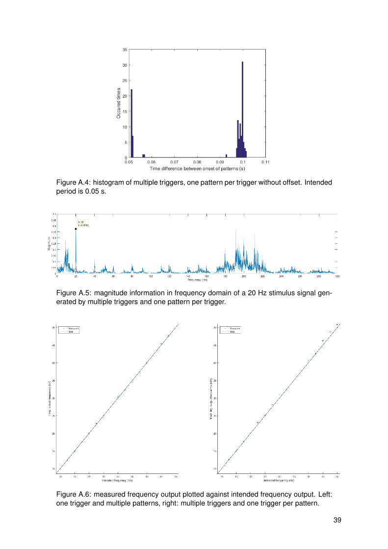
Figure A.4: histogram of multiple triggers, one pattern per trigger without offset. Intendedperiod is 0.05 s.

Figure A.5: magnitude information in frequency domain of a 20 Hz stimulus signal gen-erated by multiple triggers and one pattern per trigger.

Figure A.6: measured frequency output plotted against intended frequency output. Left:one trigger and multiple patterns, right: multiple triggers and one trigger per pattern.

39

B. Fourier series analysis

Using Fourier series, a function which satisfies the Dirichlet conditions can be represented as asum of multiple sine and cosine with different frequencies. Such analysis would be beneficial togive an analytical expression to a signal which is otherwise hard to transform to the frequencydomain using Laplace or Fourier transforms, since cosine and sine have an easy to work withfrequency domain representation.

The Fourier transform is calculated by: f(t) = a0 +∞∑n=1

(ancos(2πnf0t)+bnsin(2pinf0t)

)with:a0 = 1

T

∫ t0+Tt0

f(t)dt

an = 2T

∫ t0+Tt0

f(t)cos(2πnf0t) dt

bn = 2T

∫ t0+Tt0

f(t)sin(2πnf0t) dt

Fourier series of a block wave

An infinitely periodic square wave signal is considered (Figure B.1): x(t) =

if 0 ≤ t ≤W 1if W < t < T 0

with x(t) = x(t± nT ), n ∈ Z

Figure B.1: square wave signal with amplitude 1, pulsewidth W and period T.

From this signal the coefficients of the Fourier series can be calculated.

a0 = 1T

∫ t0+Tt0

f(t)dt = 1T

∫W0 1 dt = 1

T [t]W0 = WT

an = 2T

∫ t0+Tt0

f(t)cos(2πnf0t) dt = 2T

∫W0 1 cos(2πnf0t) dt = 2

T

[1

2πnf0sin(2πnf0t)

]W0

=

= 1πnf0T

[sin(2πnf0W )− sin(0)

]= 1

πnsin(2πnf0W )

In the special case where W = T2 , this results in: an = sin(πn) = 0.

bn = 2T

∫ t0+Tt0

f(t)sin(2πnf0t) dt = 2T

∫W0 1 sin(2πnf0t) dt = 2

T

[ −12πnf0

cos(2πnf0t)]W0

=

40

= −1πnf0T

[cos(2πnf0W )− cos(0)

]= 1−cos(2πnf0W )

πn

In the special case where W = T2 , this results in: an = 1−cos(πn)

πn , which is for 0 for even n and2πn for odd n.

The coefficients result in a Fourier series of signal x(t) which is expressed as:

x(t) = WT +

∞∑n=1

( 1

πnsin(2πnf0W )cos(2πnf0t) +

1− cos(2πnf0W )

πnsin(2πnf0t)

)=

x(t) = WT +

∞∑n=1

( 1

πnsin(2πnf0W )cos(2πnf0t)−

1

πncos(2πnf0W )sin(2πnf0t)+

1

πnsin(2πnf0t)

)Using the trigonometric angle sum identity sin(a ± b) = sin(a)cos(b) ± cos(a)sin(b), x(t) canbe rewritten:

x(t) = WT +

∞∑n=1

( 1

πnsin(2πnf0(W − t)) +

1

πnsin(2πnf0t)

)In the case w = T

2 , the expression reduces to:

x(t) = 12 +

∞∑n=1

( 1

πnsin(2πnf0

T

2)cos(2πnf0t)−

1

πncos(2πnf0

T

2)sin(2πnf0t) +

1

πnsin(2πnf0t)

)

x(t) = 12 +

∞∑n=1

( 1

πnsin(πn)cos(2πnf0t)−

1

πncos(πnf0)sin(2πnf0t) +

1

πnsin(2πnf0t)

)

x(t) = 12 +

∞∑n=1

(− 1

πncos(πnf0)sin(2πnf0t) +

1

πnsin(2πnf0t)

)This expression can be separated for n even or odd. For even multiples of n:

x(t) = 12 +

∞∑n=2,4,...

(− 1

πnsin(2πnf0t) +

1

πnsin(2πnf0t)

)=

1

2

and for odd multiples of n:

x(t) = 12 +

∞∑n=1,3,...

( 1

πnsin(2πnf0t) +

1

πnsin(2πnf0t)

)=

1

2+

∞∑n=1

( 2

πnsin(2πnf0t)

)

Derivation of modulated pulse train

A derivation for the Fourier series of a square wave with arbitrary duty cycle and a 50% dutycycle have been made. These will be used to express a modulated pulse train. The pulse traincould be described as an infinitely long square wave with a small duty cycle. The modulationof this signal could be done by multiplying the signal with a 50% duty cycle square wave ofinfinite length with a lower frequency. To be consistent, this only works in the case where thefrequency of the modulating wave is an integer multiple of the frequency of the pulses. In othercases, phase shifts will occur and some pulses will be smaller than others.

The pulse train is described by signal xp, the modulation block wave is described by xm andthe modulated pulse train is described by xmp, where:

xp(t) = WTp

+

∞∑n=1

( 1

πnsin(2πnfp(W − t)) +

1

πnsin(2πnfpt)

)41

xm(t) = 12 +

∞∑k=1

( 2

πksin(2πkfmt)

), k ∈ 1, 3, 5, ...

xmp(t) = xpxm

The signal xmp can be written out:

xmp(t) = xpxm =

(WTp

+∞∑n=1

( 1

πnsin(2πnfp(W−t))+

1

πnsin(2πnfpt)

))(1

2+∞∑k=1

( 2

πksin(2πkfmt)

))

xmp(t) = W2Tp

+WTp

∞∑k=1

( 2

πksin(2πkfmt)

)+

1

2

∞∑n=1

( 1

πnsin(2πnfp(W−t))+

1

πnsin(2πnfpt)

)+

+

( ∞∑n=1

( 1

πnsin(2πnfp(W − t)) +

1

πnsin(2πnfpt)

))( ∞∑k=1

( 2

πksin(2πkfmt)

))The last part in the sum for xmp can be rewritten:( ∞∑n=1

( 1

πnsin(2πnfp(W − t)) +

1

πnsin(2πnfpt)

))( ∞∑k=1

( 2

πksin(2πkfmt)

))=

∞∑n=1

∞∑k=1

2

π2nk

(sin(2πnfp(W − t))sin(2πkfmt) + sin(2πnfpt)sin(2πkfmt)

)The trigonometric identity sin(a)sin(b) = 1

2

[cos(a− b)− cos(a+ b)

]can be used twice here.

∞∑n=1

∞∑k=1

2

π2nk

(sin(2πnfp(W − t))sin(2πkfmt) + sin(2πnfpt)sin(2πkfmt)

)=

∞∑n=1

∞∑k=1

1

π2nk

(cos(2π(nfp(W−t)−kfmt)

)−cos

(2π(nfp(W−t)+kfmt)

)+cos

(2πt(nfp−kfm)

)−

cos(2πt(nfp + kfm)

))If W = T

2 , the expression above would result in twice the last two cosine terms for n odd andzero for n even.

The expression for xmp can now be rewritten into:

xmp(t) = W2Tp

+ WTp

∞∑k=1

( 2

πksin(2πkfmt)

)+

1

2

∞∑n=1

( 1

πnsin(2πnfp(W − t)) +

1

πnsin(2πnfpt)

)+

∞∑n=1

∞∑k=1

1

π2nk

(cos(2π(nfp(W−t)−kfmt)

)−cos

(2π(nfp(W−t)+kfmt)

)+cos

(2πt(nfp−kfm)

)−

cos(2πt(nfp + kfm)

))This expression shows that periodic functions with different frequencies are present in signalxmp(t): fm and integer multiples, fp and integer multiples and linear combinations of integermultiples of fm and fp.

To let a Fourier series describe the behavior of a signal, the signal should be periodic for infinitetime. This is off course not possible in reality, but the signal can be made more realistic. Themodulated pulse train is active for several seconds and inactive for the next several seconds.For the calculation, these times are considered equal. This would mean that the modulatedpulse train is again modulated with a 50% duty cycle square wave which has a lower frequencythan both fundamental frequencies of xp and xm. The fundamental frequency of this lastsquare wave would be less than 1 Hz, since a modulated pulse train will last for longer than

42

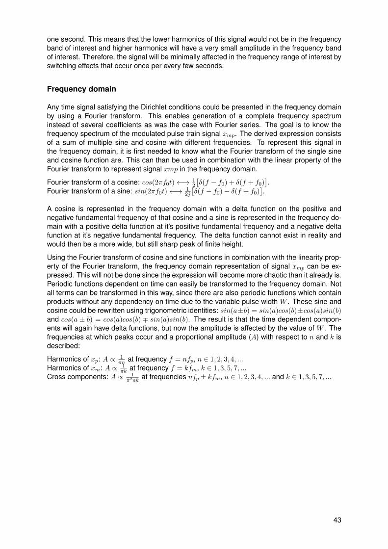
one second. This means that the lower harmonics of this signal would not be in the frequencyband of interest and higher harmonics will have a very small amplitude in the frequency bandof interest. Therefore, the signal will be minimally affected in the frequency range of interest byswitching effects that occur once per every few seconds.

Frequency domain

Any time signal satisfying the Dirichlet conditions could be presented in the frequency domainby using a Fourier transform. This enables generation of a complete frequency spectruminstead of several coefficients as was the case with Fourier series. The goal is to know thefrequency spectrum of the modulated pulse train signal xmp. The derived expression consistsof a sum of multiple sine and cosine with different frequencies. To represent this signal inthe frequency domain, it is first needed to know what the Fourier transform of the single sineand cosine function are. This can than be used in combination with the linear property of theFourier transform to represent signal xmp in the frequency domain.

Fourier transform of a cosine: cos(2πf0t)←→ 12

[δ(f − f0) + δ(f + f0)

].

Fourier transform of a sine: sin(2πf0t)←→ 12j

[δ(f − f0)− δ(f + f0)

].

A cosine is represented in the frequency domain with a delta function on the positive andnegative fundamental frequency of that cosine and a sine is represented in the frequency do-main with a positive delta function at it’s positive fundamental frequency and a negative deltafunction at it’s negative fundamental frequency. The delta function cannot exist in reality andwould then be a more wide, but still sharp peak of finite height.

Using the Fourier transform of cosine and sine functions in combination with the linearity prop-erty of the Fourier transform, the frequency domain representation of signal xmp can be ex-pressed. This will not be done since the expression will become more chaotic than it already is.Periodic functions dependent on time can easily be transformed to the frequency domain. Notall terms can be transformed in this way, since there are also periodic functions which containproducts without any dependency on time due to the variable pulse width W . These sine andcosine could be rewritten using trigonometric identities: sin(a±b) = sin(a)cos(b)±cos(a)sin(b)and cos(a ± b) = cos(a)cos(b) ∓ sin(a)sin(b). The result is that the time dependent compon-ents will again have delta functions, but now the amplitude is affected by the value of W . Thefrequencies at which peaks occur and a proportional amplitude (A) with respect to n and k isdescribed:

Harmonics of xp: A ∝ 1πn at frequency f = nfp, n ∈ 1, 2, 3, 4, ...

Harmonics of xm: A ∝ 1πk at frequency f = kfm, k ∈ 1, 3, 5, 7, ...

Cross components: A ∝ 1π2nk

at frequencies nfp ± kfm, n ∈ 1, 2, 3, 4, ... and k ∈ 1, 3, 5, 7, ...

43

ONDERWERP Datum: 06-06-2016 Informatie wetenschappelijke pilotstudie TITEL ONDERZOEK Frequency tagging of electrocutaneous stimuli for observation of corticical nociceptive processing Geachte heer/mevrouw, Onlangs bent u benaderd voor deelname aan het hierboven genoemde onderzoek en hebt al het een en ander uitgelegd gekregen. Wij vragen u vriendelijk om mee te doen aan dit wetenschappelijke onderzoek. U beslist zelf of u wilt meedoen. Voordat u de beslissing neemt, is het belangrijk om meer te weten over het onderzoek. Daarom ontvangt u deze schriftelijke informatie. Leest u deze informatie rustig door en bespreek het met partner, vrienden of familie. Als u nog vragen heeft kunt u terecht bij de onderzoeker (zie contactinformatie onderaan deze brief). Wat is het doel van het onderzoek? Chronische pijn is een veelvoorkomend probleem. In Nederland zijn er jaarlijks 150.000 tot 200.000 patiënten die langdurige pijn overhouden na een operatie. De kwaliteit van leven is bij patiënten met chronische pijn lager dan bij gezonde mensen. Aan de Universiteit Twente wordt onderzoek gedaan naar de manier waarop het zenuwstelsel pijninformatie verwerkt. In dit onderzoek doen we dat door elektrische stimuli met verschillende eigenschappen toe te dienen en daarbij de hersenactiviteit te meten met elektroden op de hoofdhuid (EEG). De stimuli zult u voelen als kleine prikjes op de huid en de hersenactiviteit geeft informatie over de verwerking van deze stimuli. Tevens wordt er bijgehouden hoe pijnlijk u de stimuli ervaart. Hiermee kunnen we onder andere de intensiteitsdrempel bepalen. Met deze informatie kunnen we de werking van het pijnsysteem onderzoeken om meer te weten te komen over hoe het pijnsysteem bij gezonde personen en bij chronische pijn patiënten werkt. Zo hopen we uiteindelijk acute en chronische pijn van elkaar te kunnen onderscheiden en daarmee diagnostische methoden te creëren om pijnpatiënten in een vroeg stadium, voordat de pijn chronisch wordt, te kunnen helpen. Hoe wordt het onderzoek uitgevoerd? Voor dit onderzoek vragen wij u één keer naar het gebouw de Horst op de Universiteit Twente te komen. Als proefpersoon krijgt u een elektrode met 5 kleine naaldjes op de rug van uw hand. Deze naaldjes prikken niet door de huid. De elektrode geeft kleine elektrische pulsjes waardoor een milde prikkende pijnsensatie ontstaat. De intensiteit van de stimuli is zo laag dat u de stimuli net wel of net niet zult voelen. Op uw bovenarm wordt een electrode met een wat grotere oppervlakte geplakt welke verder geen effect heeft op het gevoel. Verder wordt er een soort badmuts opgezet met elektroden die de hersenactiviteit (EEG) meten. In de 64 elektroden van deze badmuts wordt een geleidende gel gespoten met een naald met stompe punt, zodat de elektroden goed contact maken met uw hoofdhuid. U mag plaatsnemen in een gemakkelijke stoel en uw aandacht richten op een punt op de muur, zodat de meting minimaal wordt verstoord. Op de hand waar geen elektrode is geplakt krijgt u een kastje met een knop. Als u de knop indrukt volgt er kort daarop een elektrische prikkel die u net wel of net niet zult voelen. Eerst zal een gevoelsdrempel worden bepaald. Zodra u een prikkel voelt laat u zo snel mogelijk de knop los. Als de drempelwaarde is bepaald zullen de elektrische prikkels langer worden (10 s). Deze prikkels zullen gebruikt worden voor signaalanalyse na het experiment. U krijgt in ongeveer een half uur stimuli toegediend. Tussendoor kunt u zelf bepalen wanneer u wilt rusten. Het geheel zal ongeveer 1,5 uur duren inclusief voorbereiding. Wanneer bent u geschikt voor het onderzoek? U bent geschikt voor het onderzoek als u:

Ouder bent dan 18 jaar

Gezond bent

Geen pijn heeft Wanneer bent u niet geschikt voor het onderzoek?

C. Subject information letter

44

U bent niet geschikt voor het onderzoek als u:

Pijn heeft

Een huidaandoening heeft (met name op de handen)

Zwanger bent

Geïmplanteerde elektronische apparaten heeft, zoals een pacemaker of deep brain stimulator.

Wat wordt er van u verwacht? We verwachten van u dat u een aantal leefregels hanteert vóór het onderzoek:

Gebruik geen opwekkende of verdovende middelen (zoals koffie of alcohol) vanaf 24 uur voor het onderzoek.

Zorg voor voldoende slaap vóór de dag van het onderzoek.

Op de dag van het onderzoek: voorafgaand aan de meting goed ontbijten en/of lunchen. Welke bijwerkingen kunt u verwachten? Er zijn geen verwachte bijwerkingen en/of risico’s door deelname aan dit onderzoek. De elektrode kan na de metingen een aantal uur tot een dag rode puntjes op de huid achter laten. Daarnaast kan de naald waarmee gel op de hoofdhuid wordt gespoten even gevoelig zijn bij het wegkrassen van wat dode huidcellen. Dit kan een rode plek op de huid achterlaten welke niet langer dan een aantal uur te zien zal blijven. Wat zijn de mogelijke voor- en nadelen van deelname aan dit onderzoek? Deelname aan dit onderzoek levert u geen direct voordeel op. Voor de toekomst kan uw bijdrage echter zeer nuttige gegevens opleveren over hoe pijn wordt verwerkt door het lichaam. Wat er gebeurt er als u niet wenst deel te nemen aan dit onderzoek? U beslist zelf of u meedoet aan het onderzoek. Deelname is vrijwillig. Als u besluit niet mee te doen, hoeft u verder niets te doen. U hoeft niets te tekenen. U hoeft ook niet te zeggen waarom u niet wilt meedoen. Als u wel meedoet, kunt u zich altijd bedenken en toch stoppen. De onderzoeker is verplicht te vragen wat de reden is dat u stopt. Hierop bent u niet verplicht te antwoorden. Mocht u het niet eens zijn met bepaalde procedures dan behoudt u het recht om dit de onderzoeker te melden. Wat gebeurt er als het onderzoek is afgelopen? Deelname aan dit onderzoek kan om verschillende redenen beëindigd worden. Ten eerste kunt u zelf te allen tijde aangeven om met het onderzoek te stoppen. Hiervoor hoeft u geen reden aan te voeren. De onderzoeker kan ook besluiten om uw deelname aan het onderzoek te beëindigen. Dit kan bijvoorbeeld om gezondheidsredenen zijn of als u zich niet kan/wil houden aan de leefregels van het onderzoek. Het beëindigen van deelname levert geen risico’s op. Wat gebeurt er met uw gegevens? Als u deelneemt aan het onderzoek, dan worden tijdens de metingen gegevens over u verzameld. Uw gegevens worden alleen gebruikt voor onderzoek en zullen nooit vrijgegeven worden. U zult in geen enkele publicatie of presentatie over het onderzoek worden geïdentificeerd. Wilt u verder nog iets weten? Per mail en telefoon is de onderzoeker, Sjoerd Nijhof, bereikbaar voor verdere vragen en opmerkingen. Tijdens de experimenten wordt u nogmaals ingelicht over de procedure. Wij danken u bij voorbaat voor uw medewerking. Met vriendelijke groet, Sjoerd Nijhof Bacheloropdracht student MIRA Institute for Biomedical Technology and Technical Medicine Biomedische Signalen en Systemen Faculteit Elektrotechniek, wiskunde en informatica Universiteit Twente Zuidhorst, kamer 207 Tel: 0613432146 s.f.j.nijhof@student.utwente.nl

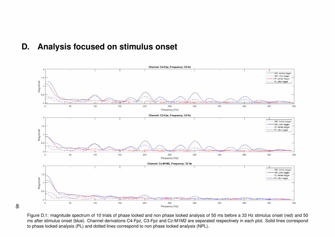
D. Analysis focused on stimulus onset

Figure D.1: magnitude spectrum of 10 trials of phase locked and non phase locked analysis of 50 ms before a 33 Hz stimulus onset (red) and 50ms after stimulus onset (blue). Channel derivations C4-Fpz, C3-Fpz and Cz-M1M2 are separated respectively in each plot. Solid lines correspondto phase locked analysis (PL) and dotted lines correspond to non phase locked analysis (NPL).

46

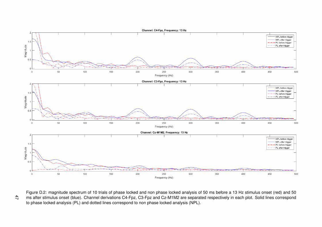
Figure D.2: magnitude spectrum of 10 trials of phase locked and non phase locked analysis of 50 ms before a 13 Hz stimulus onset (red) and 50ms after stimulus onset (blue). Channel derivations C4-Fpz, C3-Fpz and Cz-M1M2 are separated respectively in each plot. Solid lines correspondto phase locked analysis (PL) and dotted lines correspond to non phase locked analysis (NPL).

47

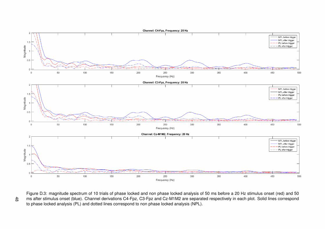
Figure D.3: magnitude spectrum of 10 trials of phase locked and non phase locked analysis of 50 ms before a 20 Hz stimulus onset (red) and 50ms after stimulus onset (blue). Channel derivations C4-Fpz, C3-Fpz and Cz-M1M2 are separated respectively in each plot. Solid lines correspondto phase locked analysis (PL) and dotted lines correspond to non phase locked analysis (NPL).

48

Figure D.4: magnitude spectrum of 10 trials of phase locked and non phase locked analysis of 50 ms before a 43 Hz stimulus onset (red) and 50ms after stimulus onset (blue). Channel derivations C4-Fpz, C3-Fpz and Cz-M1M2 are separated respectively in each plot. Solid lines correspondto phase locked analysis (PL) and dotted lines correspond to non phase locked analysis (NPL).

49

50