Embed Size (px)
Citation preview
Journal of Colloid and Interface Science 254, 372–383 (2002)doi:10.1006/jcis.2002.8596
Frequency-Dependent Electroosmosis
Philip M. Reppert1 and Frank Dale Morgan
Earth Resources Laboratory, Department of Earth Atmospheric and Planetary Sciences, MassachusettsInstitute of Technology, 42 Carleton Street, Cambridge, Massachusetts 02142
Received January 23, 2002; accepted July 12, 2002
This paper presents a theory for frequency-dependent electroos-mosis. It is shown that for a closed capillary the electroosmosisfrequency-dependent ratio of �V/�P is constant with increasingfrequency until inertial effects become prevalent, at which time�V/�P starts to decrease with increasing frequency. The frequencyresponse of the electroosmosis coupling coefficient is shown to bedependent on the capillary radius. As the capillary radius is madesmaller, inertial effects start to occur at higher frequencies. As partof this paper, frequency-dependent electroosmosis is compared tofrequency-dependent streaming potentials. In this comparison it isshown that inertial effects start to become more prevalent at higherfrequencies for the closed capillary frequency-dependent electroos-mosis case than for the frequency-dependent streaming potentialcase in the same capillary. It is also shown that this difference isdue to a second viscosity (transverse) wave that emanates from thevelocity zero within the capillary for the electroosmosis case. Thesecond viscosity wave superposes with the viscosity wave that em-anates from wall of the capillary to effectively reduce the hydraulicradius of the capillary. Data are presented for a 0.127-mm capillaryto support the findings in this paper. C© 2002 Elsevier Science (USA)
I. INTRODUCTION
Electroosmosis, the movement of a fluid with respect to acharged solid wall when an electric field is applied tangentiallyto the charged solid wall, has been studied for many years asdiscussed by Hunter (1). Frequency-dependent electroosmosis(FDE), the study of electroosmosis when the applied electricfield has a frequency component, has only recently been studied(2). There are many potential reasons for studying frequency-dependent electroosmosis ranging from medicine to geophysics.In medicine, electroosmosis has been used to study a variety ofhuman processes (3, 4). However, new areas of study may berelated to the effects of AC electroosmosis on humans, suchas electricians working in close proximity to high-voltage acelectromagnetic (EM) fields or the effects of cellular phone EMfields on human brains.
1 To whom correspondence should be addressed at Department of GeologicalSciences, 338 Brackett Hall, Clemson University, Clemson, SC 29634. E-mail:[email protected].
370021-9797/02 $35.00C© 2002 Elsevier Science (USA)All rights reserved.
In the geosciences, there has been interest in streaming po-tentials as related to earthquake phenomena (5, 6). There hasalso been recent work, which suggests that frequency-dependentstreaming potentials may be useful for determining the perme-ability of rocks (7, 8). FDE’s counterpart, frequency-dependentstreaming potential, has been shown to be useful in determiningthe capillary diameters and the pore diameters of porous media(8, 9). This leads to another reason for studying FDE, which isthe potential to use FDE to study fluid flow in capillaries andporous media.
Frequency-dependent electroosmosis may have significantadvantages over frequency-dependent streaming potentials forthe study of fluid flow, due to the differences in the �V/�Pproperties of both phenomena. The streaming potential couplingcoefficient is the ratio of the measured streaming potential volt-age to the pressure applied across the sample (i.e., �Vm/�Pa):the subscripts “m” and “a” stand for the measured and applied,respectively. The frequency-dependent streaming potential cou-pling coefficient decreases when inertial effects within the fluidstart to become prevalent as the frequency is increased. Thiscauses the induced voltage to decrease relative to the pressureapplied across the sample. This situation can be problematic inthe approximate frequency range of 500 Hz to 10 kHz. In this fre-quency range, pressure-generating devices are very inefficient,making it difficult to generate pressures large enough to inducemeasurable streaming potential signals.
The frequency-dependent electroosmosis coupling coefficient(�V/�P), as defined in this paper, is the ratio of the voltage ap-plied across the sample to the induced pressure measured acrossthe sample (�Va/�Pm). This coupling coefficient is not to beconfused with Onsager’s relations (10). This research has shownthat the FDE coupling coefficient, like the frequency-dependentstreaming potential coupling coefficient, decreases as the fre-quency is increased past the rollover frequency. The rolloverfrequency is the frequency at which the coupling coefficient is98% of its dc value. However, there is a significant practicaldifference between the coupling coefficient, as defined in thispaper, for the streaming potential and the electroosmosis cases.As the frequency is increased, the voltage applied across thesample can be more easily kept constant in magnitude for thefrequency-dependent electroosmosis case than the applied pres-sure can be kept constant in the streaming potential case. For the
2

N
FREQUENCY-DEPENDEFDE case, this has the consequence that the pressure measuredacross the sample increases as the frequency is increased pastthe rollover frequency. This has practical implications, whichwill make measurement of the pressure easier at the higher fre-quencies. In the frequency range of 500 Hz to 10 kHz, FDE maybe more useful than frequency-dependent streaming potentialsbecause �V is applied and �P is measured in the FDE case.
Also, due to the nature of the signals, it is much easier to gen-erate large amplitude voltage signals than it is to generate largeamplitude pressure signals at these frequencies.
Until recently, little attention has been paid to frequency-dependent electroosmosis. Minor et al. (2) determined the char-acteristic time for dynamic electroosmosis and electrophoresis.Electrophoresis is similar to electroosmosis in that both pheno-mena use electric fields to induce motion. In electrophoresis, thefluid remains stationary while the electric field causes colloidalparticles to move tangential to the applied electric field. Minoret al. (2) provided data showing the relaxation frequency andthen fitted the data with an empirically determined curve usingthe characteristic time. Although the general shapes of the curveswere in good agreement, there was not a good correlation be-tween the theoretical and the measured relaxation frequencies,according to Minor et al. (2). Recently there have been other pa-pers on frequency-dependent/dynamic electrophoresis (11, 12),but they do not provide analytical solutions for the mobility. Inthe study of electroosmosis, the term mobility refers to −εζ/η,where ε is the permittivity of the fluid, ζ is the zeta potential,and η is the viscosity of the fluid.
This paper provides the theoretical development of an an-alytical solution for frequency-dependent electroosmosis in acapillary. First a brief review of dc electroosmosis is presented,followed by the theory of frequency-dependent electroosmo-sis. The theory is developed from the Navier–Stokes equationbecause this approach allows for a better understanding of thephysics behind FDE. The FDE theory is then compared to thefrequency-dependent streaming potential theory to facilitate un-derstanding the underlying physics of FDE. Last, experimentaldata collected by the authors is presented to verify the theory.
II. DC ELECTROOSMOSIS
Direct current electroosmosis has been studied in its presentform since originally presented by von Smoluchowski in 1921(13). In dc electroosmosis an electric field is applied tangentiallyto a charged surface in contact with an ionic fluid, causing thefluid to move parallel to the surface. The fluid is displaced whenthe electric field moves the ions in the diffuse part of the electri-cal double layer, which is adjacent to the surface. A simplifiedschematic representation of the Stern (14) model of the electri-cal double layer is shown in Fig. 1. The zeta (ζ ) potential is thepotential at the slipping plane (S), the potential at the surface isϕo, and ϕd is the potential at the Stern plane (OH). The potential
in the diffuse region decays exponentially from the Stern layerinto the bulk fluid as shown in Fig. 1. An abundance of cationsT ELECTROOSMOSIS 373
FIG. 1. (a) Simplified schematic representation of the electrical double layerwhere OH is the outer Helmholtz or Stern plane, S is the slipping plane, andthe diffuse zone is represented by a diminished number of ions. (b) Simplifiedschematic representation of the potential distribution in the electrical doublelayer, where ϕ0 is the potential at the surface, ϕd is the potential at the Sternplane, and ζ is the potential at the slipping plane.
(or anions) compared to anions (or cations) near the Stern layercauses the potential to decay into the bulk fluid where the fluidis electrically neutral. Consequently, as the electric field movesthe ions, viscous forces in the fluid near the surface pull the fluidalong with the ions. This can be seen in Fig. 2, which is a modi-fied version of Hunter’s (13) figure. For a charged planar surfacewhere an electric field is applied tangential to the surface, theequation governing dc electroosmosis is
ηd2vz
dx2= Ezρc(x), [1]
where Ez is the electric field applied tangentially to the surface,ρc(x) is the charge density, η is the viscosity of the fluid, vz(x) isthe dc electroosmotic fluid velocity, and x is the distance fromthe surface. Applying Poison’s equation to substitute for ρc(x),Eq. [1] can be rewritten as
ηd2vz(x)
dx2= Ezε
d2ϕ(x)
dx2, [2]
where ϕ(x) is the potential, and ε is the permittivity of the fluid.Solving this differential equation with the boundary conditions

that dc electroosmosis is a special case of frequency-dependent
374 REPPERT AN
that dϕ/dx = 0 and dvz/dx = 0 in the bulk fluid and ϕ = ζ andvz = 0 at the slipping plane gives
vz(x) = ε
ηEz[ϕ(x) − ζ ]. [3]
With the substitution of the Debye–Huckel approximation,ϕ(x) = ζ exp(−κx), for the potential distribution, Eq. [3] be-comes
vz(x) = εζ
ηEz[exp(−κx) − 1], [4]
which is often approximated by
vz = −εζ
ηEz. [5]
This approximation holds at a distance of 3 Debye lengthsand greater from the wall (any distance beyond the double layer)where the fluid velocity is essentially a constant. This can be seenwhen plotting Eq. [4], as shown in Fig. 3, where the constantvelocity is achieved at approximately 3/κ and 1/κ is the Debyescreening length. The Debye screening length is the distance atwhich the potential has decreased by a factor of 2.718 (e) and isgiven by 1/κ , where κ is the Debye–Huckel parameter whoseapproximation (13) is given by
κ =(
103(2z2e2 If NA)
εkBT
) 12
, [6]
where z is the valence of the ions, e the is elementary charge, If
FIG. 2. Simplified schematic representation of electroosmotic flow in openand closed capillaries. In the open capillary (a), the electroosmotic flow isshown as a plug flow, which has its maximum velocity at approximately3 Debye lengths from the wall. In the closed capillary (b), the electroosmotic
flow must be balanced by a counterflow. The actual fluid velocity is the sum ofthe electroosmotic flow and the counterflow.D MORGAN
FIG. 3. DC electroosmotic velocity profile in a capillary from the wall tothe center of the capillary. At approximately 3 Debye lengths from the wall thefluid is at its maximum velocity.
is the ionic strength of the fluid, NA is Avogadro’s constant, kB isthe Boltzmann constant, and T is the temperature in Kelvins. Theapproximation made in Eq. [5] holds because in electroosmosis,we are often concerned with measuring the fluid velocity in thebulk fluid for an open capillary or measuring the counterpressurefor a closed capillary. In the open capillary case, the fluid velocityis constant in the bulk fluid as given by Eq. [5]. In the closedcapillary case the counterpressure is generated by the volumeflow in the capillary. The fluid volume within 3 Debye lengthsof the wall is infinitesimal compared to the volume in the bulkfluid provided that the capillary radius is large compared to theDebye length. Consequently, the bulk fluid response controls thefluid response.
In a closed capillary, the electroosmotic flow induces a coun-terpressure gradient. The counterpressure gradient generates abackflow whose volume flow must balance the electroosmoticvolume flow. This is seen schematically in Fig. 2b, which showsthe electroosmosis flow profile and the counterflow velocity pro-files. The electroosmosis dc coupling coefficient is found bysetting the electroosmosis volume flow equal to the counter-volume-flow and taking the ratio �V/�P , which gives
�V
�P= x2
8εζ. [7]
III. FREQUENCY-DEPENDENT ELECTROOSMOSIS
Having done a brief review of dc electroosmosis, frequency-dependent electroosmosis is now examined. It should be noted
electroosmosis where the frequency and phase are zero. As in

N
FREQUENCY-DEPENDEthe dc case an electric field is applied tangentially to a chargedsurface that is in contact with an ionic fluid. However, theelectric field is now time varying. The frequency-dependentelectroosmosis force balance equation that describes this case is
ρ∂
∂t{vz(x)e[i(ωt + θ )]}
= η∂2
∂x2{vz(x) exp[i(ωt + θ )]} − ε
∂2ϕ(x)
∂x2Ez exp[iωt], [8]
where Ez exp(iωt) is the sinusoidal forcing function,vz(x) exp[i(ωt + θ )] is the sinusoidal response with an unknownphase (θ ), and ρ is the density of the fluid. Introducing phasornotation into the problem, which is often used in electrical en-gineering,
v = vz exp[i(ωt + θ )] = w + iy, [9]
where vz is a real vector and v is a complex vector with areal component w = Re(v) and imaginary component y = Im(v).Taking the derivative with respect to time of the left side ofEq. [8], and using phasor notation, which utilizes the Fouriertransform and allows the equation to be viewed in the frequencydomain, Eq. [8] can now be represented as
iρωv(x, ω) = η∂2v(x, ω)
∂x2− ε
∂2ϕ(x)
∂x2E(ω). [10]
This equation is essentially a modified form of the Navier–Stokesequation,
ρd v
dt= η∇2v + B − ∇ P, [11]
where the first term of Eqs. [8] and [10] is the fluid densitymultiplied by the acceleration of the fluid to give the inertialforces, which equates to the first term of Eq. [11]. The secondterm in Eqs. [8] and [10] represents the viscous forces in the fluid,which equates to the second term in Eq. [11], which is also theviscous forces. The third term in Eqs. [8] and [10] representsthe forces due to the electric field. This term equates to the thirdterm in Eq. [11], which is the body forces on the fluid. Thelast term in Eq. [11], the pressure gradient, does not appear inEqs. [8] and [10] because the solution is for an open capillary. Itcan be seen in the earlier development of dc electroosmosis inthis paper or in the development of dc electroosmosis by a varietyof other authors such as Hunter (13) that a pressure gradient doesnot exist in an open capillary solution.
When examining the time-independent/static (dc) case,Eq. [1], it is seen that the viscous forces must equal the electricfield forces. However, in the frequency-dependent case, inertialforces must now be included in the solution. This can be seen in
Eq. [8] where the second and third terms are the same as in thedc case except that now the terms are time varying due to theT ELECTROOSMOSIS 375
time varying forcing function in the third term. The first term ofEq. [8] becomes an inertial term, due to the time varying func-tion. Whereas, in the dc case where ω equals zero, the derivativewith respect to time vanishes for the first term of Eq. [8]. In theac case the first term is differentiable and remains as the inertialterm. Upon examination of Eq. [8], it is obvious that it does nothave an exact analytical solution because there is one equationand two unknowns. This difficulty was overcome by solving theequation in two different regions within the capillary, one nearthe wall and the other in the bulk fluid. In order for this solutionto be valid, certain restrictions are required.
The main restriction of this solution is that the viscous skindepth (9, 15),
δ =√
η
ρω, [12]
cannot approach within 3 Debye lengths of the wall. The vis-cous skin depth is the distance away from the no-flow boundarycondition at the wall to where the vorticity wave has been at-tenuated by a factor of 2.718 (e). The solution to Eq. [10] isrestricted to frequencies less then 1 MHz and to solutions withconcentrations greater than 10−4 M. These restrictions ensurethat there are no inertial effects within 3 Debye lengths of thewall. As part of this solution, it is assumed that the capillary issufficiently long that end effects can be neglected.
A. Near-Wall Solution
The near-wall solution is for the region between the no-flowcondition at the wall (slipping plane) and 3 Debye lengths awayfrom the wall. Within this region the radius of curvature is neg-ligible; therefore, the geometry of the capillary is not includedin the near-wall solution. Also, as stated earlier in the discus-sion concerning the restrictions to the solution, there cannotbe any inertial effects in the near-wall solution. Therefore, thefrequency-dependent electroosmosis governing Eq. [10] for thenear-wall solution becomes
η∂2vew(x, ω)
∂x2= ε
∂2ϕ(x)
∂x2E(ω), [13]
where vew is the electroosmotic fluid velocity near the wall. Thesolution of Eq. [13] is
vew(x, ω) = εζ
η[exp(−κx) − 1]E(ω), [14]
which is identical to the dc case except for the frequency com-ponent. When examining Eq. [14] it can be seen that the velocitynear the wall is always in phase with the driving electric field. It
can also be seen that the velocity reaches a maximum at 3 Debyelengths from the wall just as in the dc case.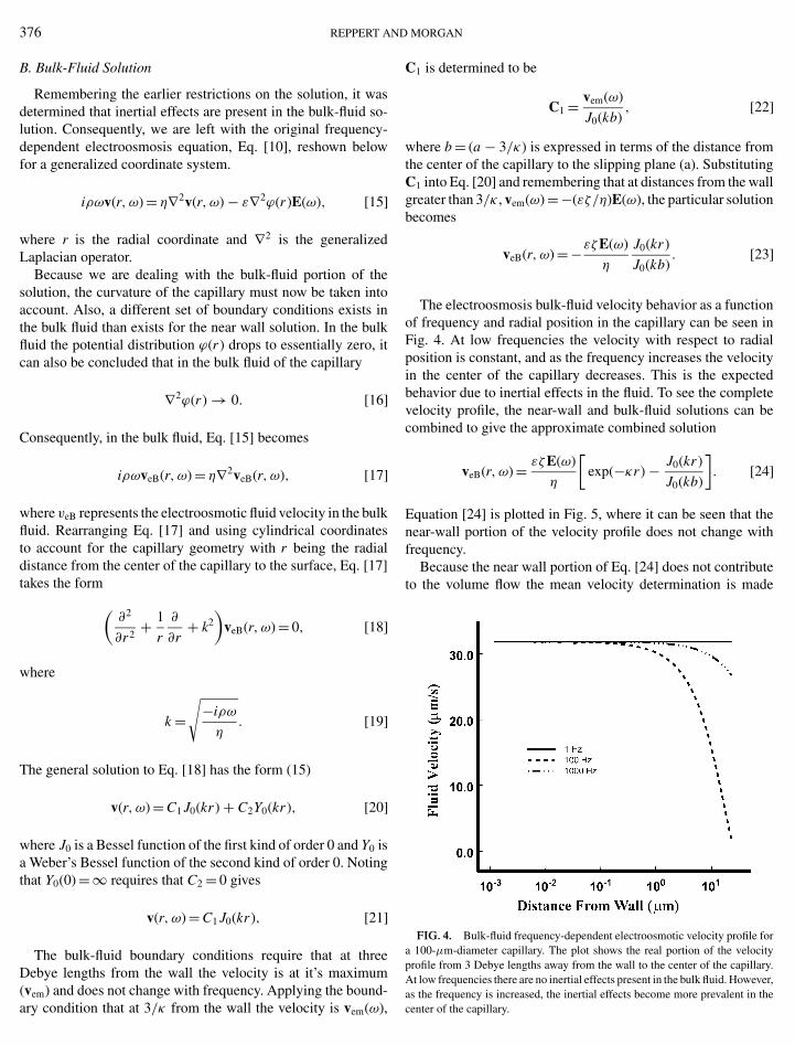
376 REPPERT AN
B. Bulk-Fluid Solution
Remembering the earlier restrictions on the solution, it wasdetermined that inertial effects are present in the bulk-fluid so-lution. Consequently, we are left with the original frequency-dependent electroosmosis equation, Eq. [10], reshown belowfor a generalized coordinate system.
iρωv(r, ω) = η∇2v(r, ω) − ε∇2ϕ(r )E(ω), [15]
where r is the radial coordinate and ∇2 is the generalizedLaplacian operator.
Because we are dealing with the bulk-fluid portion of thesolution, the curvature of the capillary must now be taken intoaccount. Also, a different set of boundary conditions exists inthe bulk fluid than exists for the near wall solution. In the bulkfluid the potential distribution ϕ(r ) drops to essentially zero, itcan also be concluded that in the bulk fluid of the capillary
∇2ϕ(r ) → 0. [16]
Consequently, in the bulk fluid, Eq. [15] becomes
iρωveB(r, ω) = η∇2veB(r, ω), [17]
where veB represents the electroosmotic fluid velocity in the bulkfluid. Rearranging Eq. [17] and using cylindrical coordinatesto account for the capillary geometry with r being the radialdistance from the center of the capillary to the surface, Eq. [17]takes the form
(∂2
∂r2+ 1
r
∂
∂r+ k2
)veB(r, ω) = 0, [18]
where
k =√
−iρω
η. [19]
The general solution to Eq. [18] has the form (15)
v(r, ω) = C1 J0(kr ) + C2Y0(kr ), [20]
where J0 is a Bessel function of the first kind of order 0 and Y0 isa Weber’s Bessel function of the second kind of order 0. Notingthat Y0(0) = ∞ requires that C2 = 0 gives
v(r, ω) = C1 J0(kr ), [21]
The bulk-fluid boundary conditions require that at threeDebye lengths from the wall the velocity is at it’s maximum
(vem) and does not change with frequency. Applying the bound-ary condition that at 3/κ from the wall the velocity is vem(ω),D MORGAN
C1 is determined to be
C1 = vem(ω)
J0(kb), [22]
where b = (a − 3/κ) is expressed in terms of the distance fromthe center of the capillary to the slipping plane (a). SubstitutingC1 into Eq. [20] and remembering that at distances from the wallgreater than 3/κ , vem(ω) = −(εζ/η)E(ω), the particular solutionbecomes
veB(r, ω) = −εζE(ω)
η
J0(kr )
J0(kb). [23]
The electroosmosis bulk-fluid velocity behavior as a functionof frequency and radial position in the capillary can be seen inFig. 4. At low frequencies the velocity with respect to radialposition is constant, and as the frequency increases the velocityin the center of the capillary decreases. This is the expectedbehavior due to inertial effects in the fluid. To see the completevelocity profile, the near-wall and bulk-fluid solutions can becombined to give the approximate combined solution
veB(r, ω) = εζE(ω)
η
[exp(−κr ) − J0(kr )
J0(kb)
]. [24]
Equation [24] is plotted in Fig. 5, where it can be seen that thenear-wall portion of the velocity profile does not change withfrequency.
Because the near wall portion of Eq. [24] does not contributeto the volume flow the mean velocity determination is made
FIG. 4. Bulk-fluid frequency-dependent electroosmotic velocity profile fora 100-µm-diameter capillary. The plot shows the real portion of the velocityprofile from 3 Debye lengths away from the wall to the center of the capillary.At low frequencies there are no inertial effects present in the bulk fluid. However,
as the frequency is increased, the inertial effects become more prevalent in thecenter of the capillary.
FREQUENCY-DEPENDE
FIG. 5. Combined near-wall and bulk-fluid FDE velocity profile for a100-µm-diameter capillary. The plot shows the real portion of the velocity profilefrom the wall (slipping plane) to the center of the capillary. At low frequenciesthere are no inertial effects present in the bulk fluid. However as the frequencyis increased, the inertial effects become more prevalent in the center of the cap-illary. It can also be seen that for all frequencies there are no inertial effects inthe near-wall region.
using veB(r, ω), from Eq. [23]. This is accomplished by inte-grating veB(r, ω) over the section of the capillary and dividingby the cross-sectional area of the capillary, giving the mean fluidvelocity as
v(ω) = 1
πa2
a∫0
2πveB(r, ω)r∂r = −εζE(ω)
η
2
ka
J1(ka)
J0(kb). [25]
Dividing the mean fluid velocity in the capillary by the elec-tric field, E(ω), we obtain the mobility for frequency-dependentelectroosmosis in an open capillary which is given as
u(ω) = v(ω)
E(ω)= −εζ
η
2
ka
J1(ka)
J0(kb)= 2udc
ka
J1(ka)
J0(kb), [26]
where udc is the mobility for the dc electroosmosis case. A plotof the frequency-dependent mobility can be seen in Fig. 6, wherethe real and imaginary portions of the response are shown fortwo different capillary sizes. The real part of Eq. [26] has a con-stant coupling coefficient until the critical frequency is reached,at which time the coupling coefficient starts to decrease withincreasing frequency. The imaginary response shows that at lowfrequencies virtually no inertial terms are present, and as thefrequency is increased the inertial terms eventually equal theviscous (real) terms. It can also be seen by using two differ-ent capillaries with radii of 100 and 500 µm that the frequencyresponse is dependent on the radius of the capillary.
To examine the frequency-dependent behavior of the electro-osmosis coupling coefficient, the volume fluid flow must be de-
NT ELECTROOSMOSIS 377
termined. This is straightforward and is achieved by integrat-ing the fluid velocity in Eq. [23] over the cross section of thecapillary,
Qe(ω) = −2π
a∫0
rveB(r, ω) ∂r, [27]
giving
Qe(ω) = −2πE(ω)εζ
η
a
k
J1(ka)
J0(kb), [28]
where Qe represents the electroosmosis volume flow. Equation[23] is used in the integration for simplicity since the exponentialterm in Eq. [24] does not contribute to the solution as discussedpreviously.
C. Counterflow Solution
As shown in Fig. 2b, if the capillary is closed at both ends, acounterflow must exist. This counterflow is driven by the pres-sure that builds up at the ends of the capillary and can be ex-pressed as,
iρωvc(r, ω) = η∇2vc(r, ω) − ∇P(ω), [29]
where vc represents the counterflow velocity and P is the drivingpressure. Eq. [29] indicates that the pressure forces are equal tothe viscous forces minus the inertial forces. Eq. [29] has beensolved numerous times in prior literature (8, 17, 18), with thesolution given as
vc(r, ω) = �P(ω)
ηlk2
[J0(kr )
J0(ka)− 1
], [30]
where l is the length of the capillary and k is the same as defined
FIG. 6. Normalized frequency-dependent mobility in a capillary, with real
and imaginary portions of the response shown for a 100- and 500-µm-diametercapillary.
378 REPPERT AN
in Eq. [19]. The volume flow is found by integrating counterflowvelocity over the area of the capillary as given by
Qc(ω) = −2π
a∫0
rvc(r, ω)∂r , [31]
giving
Qc(ω) = πa2 �P(ω)
ηlk2
[2
ka
J1(ka)
J0(ka)− 1
], [32]
where Qc is the volume flow through the capillary due to thecounterpressure.
D. Coupling Coefficient Solution
As in the dc case, the coupling coefficient is the ratio ofthe voltage applied across the sample to the pressure measuredacross the sample �Va/�Pm. Setting Qe, Eq. [28] equal to Qc,Eq. [32], and taking the ratio of �Va/�Pm gives
�V(ω)
�P(ω)= a
2εζk
(2
ka
J1(ka)
J0(ka)− 1
)/(J1(ka)
J0(kb)
), [33]
which is the ac electroosmosis coupling coefficient in a closedcapillary.
Graphically the real and imaginary response of the ac elec-troosmosis coupling coefficient for a closed capillary can be seenin Fig. 7. It can be seen that the frequency response has a formsimilar to the frequency response for the frequency-dependentmobility (Fig. 6) where the real part of Eq. [33] has a constantcoupling coefficient until the rollover frequency is reached, atwhich time the coupling coefficient starts to decrease with in-
FIG. 7. Normalized frequency-dependent electroosmosis in a closed cap-illary, with real and imaginary portions of the response shown for a 100- and
500-µm-diameter capillary. The response for the 100-µm capillary has a rolloverfrequency higher than that for the 500-µm capillary.D MORGAN
FIG. 8. The electroosmosis frequency-dependent coupling coefficient phaseresponse is shown for a 100- and a 500-µm-diameter capillary. As 45◦ is ap-proached at the high frequencies, the phase is in agreement with the real andimaginary portions of the coupling coefficient, which are approaching equalitiesequal in magnitude.
creasing frequency. The imaginary response shows that at lowfrequencies, virtually no inertial terms are present, and as thefrequency is increased the inertial terms eventually equal theviscous (real) terms. This corresponds to the coupling coef-ficient having a maximum phase response of 45◦, as shownin Fig. 8. It can also be seen in Fig. 7 that the critical fre-quency is dependent on the radius of the capillary. This canbe seen when plotting the response for two capillaries, onewith a diameter of 100 µm and the other with a diameter of500 µm. When the FDM and FDE frequency responses are com-pared using a 100-µm-diameter capillary, as seen in Fig. 9, the
FIG. 9. Comparison of normalized FDE and FDM real responses for a
100-µm and a 500-µm capillary. It can be seen that the FDE response has afrequency higher rollover than that of the FDM response.
FREQUENCY-DEPENDE
FIG. 10. Comparison of the normalized real response for FDE and FDMfor a 100-µm-diameter capillary. The response has also been normalized suchthat the inertial effects start to occur at the same frequency. It is apparent thefrequency responses are still different.
responses are not identical. In fact the electroosmosis couplingcoefficient response has a higher rollover frequency higher thanthat of the frequency-dependent mobility. As a reminder, therollover frequency is the frequency at which the coupling coef-ficient is 98% of its dc value. This frequency can be determinedfor the FDM case from (ωr = η/ρa2), which in turn can be cal-culated from the inequality |ka| < 1. For fluid movement in acapillary, Crandall (17) states that in the region where |ka| < 1,inertial forces are negligible compared to viscous forces. There-fore the rollover frequency determines the regime where inertialforces are negligible. However, this calculation for the rolloverfrequency does not hold for the FDE case. Figure 10 showsthe frequency responses of Fig. 9 normalized to the frequencywhere inertial effects start to appear in the capillary. It can beseen in Fig. 9 that the rollover frequency is different betweenthe two responses even though the frequency calculated usingthe inequality |ka| < 1 is the same for the FDE and FDM cases.
To understand better the frequency response of the frequency-dependent mobility and frequency-dependent electroosmosiscoupling coefficient it is instructive to compare them both tothe frequency-dependent streaming potential (FDSP) phenom-ena since FDSP has been more extensively studied. This isinstructive because the fluid motion in the center of the cap-illary, as a function of frequency, is controlled by inertial ef-fect for all three phenomena. To appreciate the usefulness ofthis comparison the reader should have a basic understandingof frequency-dependent streaming potentials. The theoreticalfrequency-dependent streaming potential coupling coefficient(8, 18) is given as
C(ω) = �VSP(ω)
�PSP(ω)= −
[εζ
ση
]2
ka
J1(ka)
J0(ka)= −SPDC
2
ka
J1(ka)
J0(ka),
[34]
NT ELECTROOSMOSIS 379
where C(ω) is the frequency-dependent streaming potential cou-pling coefficient which is the ratio of the voltage (�VSP) mea-sured across the sample to the differential pressure (�PSP) ap-plied across the sample and σ is the conductivity of the fluid.The remaining parameters in Eq. [34] are the same as those de-fined earlier in the paper. It should also be noted that εζ/ση isthe dc streaming potential response. The theoretical frequency-dependent streaming potential coupling coefficient, Eq. [34], isobtained by calculating the convection current
Iconv(r ) =∫
2πrvz(r )ρc(r ) dr, [35]
where vz(r ) is the fluid velocity as given in Eq. [30] and ρc(r )is the charge density as shown in Fig. 1. The convection cur-rent occurs when ions near the surface as shown in Fig. 1 arepulled along due to viscous effects in the fluid as the fluid movestangentially to the surface. This is related to the electroosmo-sis case where the ions, which are being moved by an appliedelectric field, pull the fluid along due to viscous effects in thefluid. In the streaming potential case, the convection currentmust be balanced by a conduction current to satisfy steady-state equilibrium considerations (19, 20). This is also similarto frequency-dependent electroosmosis where the two volumeflows must balance to satisfy steady-state equilibrium condi-tions. The streaming potential conduction current is determinedusing Ohm’s law where the conductance of the sample is mul-tiplied by the voltage measured across the sample, as shown inEq. [36].
Icond(r ) = πσa2
l�V [36]
The streaming potential coupling coefficient is then determinedby setting the convection current equal to the conduction cur-rent, with the ratio �V/�P taken to determine the couplingcoefficient as shown in Eq. [34].
A comparison of the FDM, FDE, and FDSP cases is nowmade. The normalized frequency responses for FDM and FDSPare identical, but the rollover frequency of the FDE case is higher.Figure 9 compares the FDE and FDM responses; it also com-pares the FDSP response to the FDE response since the FDSPand FDM responses are identical. The identical nature of theFDM and FDSP responses is further confirmed when compar-ing the governing equations, Eq. [26] and Eq. [34], respectively.In this comparison the equations are identical except for the dcportion of the response. While the FDSP and FDM frequencyresponses are identical, it is also apparent that the rollover fre-quency for the FDE response is a little more than three timeshigher in frequency than that for the FDM and FDSP responses.This difference in rollover frequency is due to the hydrodynam-ics and the viscous skin depth properties.
The differences and similarities can also be seen when lookingat Onsager’s reciprocity relations (7, 10). These relations are

380 REPPERT AN
given by
J1 = −L11∇ P − L12∇V, [37]
Jel = −L21∇ P − L22∇V, [38]
where J1 is fluid flux, Jel is the current density, L11 is thehydrodynamic permeability, L22 is the conductivity, and L12
and L21 represent the electrokinetic cross coefficients. It isshown by Lyklema (10) as well as others that the electroos-motic flux (J1/Jel)∇ P=0 = L12/L22 and the streaming potential(∇V/∇ P)Jel=0 = −L21/L22 are equal except for the sign. It canalso be shown that when Jel = J1 = 0 that
J1 = −L11∇ P − L12∇VJ1=0−→ ∇V
∇ P= − L11
L12[39]
and
Jel = −L21∇ P − L22∇VJel=0−→ ∇V
∇ P= − L21
L22. [40]
This shows that the coupling coefficient for the streamingpotential case and electroosmosis in a closed capillary case donot have the same solution, which agrees with the results shownin Figs. 9 and 10. While this result does confirm that there shouldbe a difference, it does not provide any physical insight as to whythis difference occurs. The physical meaning of this differenceis examined next.
To understand some of the differences and similarities be-tween the FDM, FDE, and FDSP frequency responses it isinstructive to look at the high-frequency response for each ofthe phenomena while revisiting the physics that is driving thephenomena. Examination of the low-frequency responses doesnot provide any additional insight since it shows that the fre-quency responses go to the DC limit as ω → 0. A comparisonof the FDM, FDE, and FDSP responses is made using high-frequency approximate solutions for the Bessel functions inthese responses.
First we discuss the FDM and FDSP cases since their fre-quency responses are identical as seen in Eq. [26] and Eq. [34],where the only difference is the DC term, which is con-stant. High-frequency Bessel function approximations can beused when ka 10, as described by Crandall (17). The high-frequency approximation used for the Bessel functions J0 andJ1 is given by
J1(x√−i)
J0(x√−i)
= −i, [41]
which can be found in Crandall (17) or which can be easilyproven using the asymptotic approximations of Abramowitz and
D MORGAN
Stegum (21). In Eq. [26]
ka = a
√− iρω
η, [42]
from which the following rearrangement is made to Eq. [38]:
x√−i = a
√− iρω
η= a
√ρω
η
√−i . [43]
Then substituting Eq. [39] into Eq. [26] gives
C(ω)ka>10
= εζ
η
[−2i
ka
]= εζ
η
−2i
a√
−iωρ
η
. [44]
Eq. [44] can then be modified to
C(ω)ka>10
= εζ
η
[−2
a
√η
ωρ
(1√2
− 1√2
i
)]. [45]
It has been previously shown (8) that the solution using Besselfunction approximations in the FDSP case is nearly identicalto the complete Bessel function solution. The high- and low-frequency approximations are identical with a slight divergencein the intermediate frequency range, 1 < ka < 10, which wasnot accounted for in the approximations. However, within thisregion, the error is smaller than measurements can detect.
The significance of Eq. [45] can fully be appreciated whencomparing it to the frequency-dependent hydraulic (FDH) high-frequency approximation as done by Reppert et al. (8), wherethe second order effect in the hydraulic response is shown to bethe driving force behind the FDSP response. The FDH trans-fer function describing the mean fluid velocity divided by thepressure measured across the capillary is given by
H(ω) = 1
iρω+ aδ
2η(1 − i)
= 1
iρω+ a
η√
2
√η
ρω
(1√2
− 1√2
i
). [46]
The bulk-fluid response is dominated by the inertial effects inthe first term. However, when frequencies are high the viscousskin depth starts to approach the wall. At this point a second-order effect given by the second term in Eq. [46] starts to domi-nate. This second-order effect shows that in the region near thewall the inertial terms are equal to the viscous terms. When wecompare Eq. [46] to Eq. [45], we see that the second-order ef-fect in the FDH case appears to dominate the whole FDSP high-frequency solution. This comes about due to the integration of
the fluid velocity and the charge density as shown in Eq. [35].The charge density is only of consequence in the vicinity of the
FREQUENCY-DEPENDE
wall and thus the bulk-fluid response has little influence on theamount of charge moved. The bulk fluid, however, does playan important role in the pressure gradient and the volume fluidflow.
As demonstrated earlier there is a similarity between the FDMand FDSP solutions given in Eqs. [26] and [34]. Understandingthe physics of FDSP then gives insight into the physics control-ling the FDM solution. It can be concluded that electroosmoticfluid motion is controlled by the near-wall interaction of theelectric field with the ions in a viscous fluid. Another way ofsaying this is that the coupling between the electric field andthe fluid is only in the near-wall region, which is the expectedconclusion for electroosmosis in an open capillary.
For the FDE high-frequency Bessel function approximation,we start with Eq. [33] and rearrange it as
�V(ω)
�P(ω)= a2
8εζ
[4
ka
(2
ka
J1(ka)
J0(ka)− 1
)/(J1(ka)
J0(ka)
)], [47]
which is a transfer function multiplied by the dc response. Ap-plying the identity of Eq. [41] to Eq. [47] we get
�V(ω)
�P(ω)= a2
8εζ
(8
k2a2− 4i
ka
)= a2
8εζ
(8ηi
a2ρω− 4
a
√iη
ρω
),
[48]
�V(ω)
�P(ω)= a2
8εζ
[8ηi
a2ρω− 4
a
√η
−iρω(1 + i)
]
= a2
8εζ
[8ηi
a2ρω+ 4
a
√η
ρω
(1√2
− 1√2
i
)]. [49]
In the FDSP, FDM, and FDE cases the very-high-frequencyresponse falls off as ω−1/2. The FDE case has another effectthat contributes to the falloff as ω−1. This effect contributesto the lower frequency portion of the high-frequency solution.The FDE transform function is caused by the superposition ofthe electroosmosis velocity profile and the counterflow velocityprofiles of Fig. 11a.
However, this does not adequately explain why the rolloverfrequency for FDE is higher than the rollover frequency forFDSP and FDM. The rollover frequency for the FDSP, FDM,and FDE cases is controlled by the viscous skin depth throughthe term
k =√
−iρω
η=
√−i
δ, [50]
where δ is the viscous skin depth as defined in Eq. [12]. In theFDSP and FDM cases, the viscosity wave emanates from thewall where the fluid velocity goes to zero.
In the FDE case there are two viscosity waves that superposeto give a resultant wave, this resultant wave describes the ve-
NT ELECTROOSMOSIS 381
FIG. 11. (a) Schematic diagram representing the velocity profile forPoiseuille flow and plug flow. The Poiseuille flow is associated with FDSPand the counterflow in FDE. The plug flow is associated with FDM and thedriving flow in FDE. (b) Schematic diagram representing electroosmosis flowin a closed capillary. It can be seen in these diagrams that the electroosmosisvelocity profile has two zeros, one at the wall and one at a distance from the wall,while the Poiseuille velocity profile has one zero at the wall. The electroosmo-sis diagram is not to scale, the 3/κ line is shown to represent an approximatedistance.
locity profiles shown in Figs. 11b and 12. A viscosity wave is atransverse wave that occurs in a fluid due to the viscosity of thefluid (15, 17). To describe a viscosity wave, the example of anoscillating plate in a viscous fluid will be used where the platehas infinite length in the y–z direction and the fluid extends in-finitely away from the plate in the x direction. As the plate is
FIG. 12. Real portion of the FDE velocity profile for a 100-µm and a500-µm diameter capillary. It can be seen that the second velocity zero does
shift with capillary size. The distance of the shift of the velocity zero is givenfor the respective curves.
382 REPPERT AN
oscillated in the y direction, the fluid is moved near the platedue to viscous forces. Due to these viscous forces a transversewave propagates into the bulk fluid with its velocity perpendic-ular to the direction of propagation. These transverse waves arerapidly damped as they move away from the plate. The veloc-ity of these waves, as given by Crandall (17) and Landau andLifschitz (15), is
vel = uo exp
(−x
√ρω
η
)exp
(i
[x√
ρω
η
]− ωt
), [51]
where the first exponential term represents the damping of thewave. As defined earlier the viscous skin depth is the distance(x) at which the wave has been damped by a value of e. There isa duality to the situation just described: instead, if we considerthe plate to be stationary and the fluid to be moving with laminarflow, the same transverse wave will emanate from the plate.
As we apply this to a capillary, the wavelength of the viscositywave is much larger than the diameter of the capillary, for thecapillary diameters and frequencies we are considering. For theFDE case there is a transverse wave emanating from the wall ofthe capillary in the shape of plug flow as shown in Fig. 11a. Thereis also a transverse wave, 180 degrees out of phase, emanatingfrom the wall caused by the counterflow, also shown in Fig. 11a.Figure 11b shows the superposition of these two waves. As canbe seen this resultant wave has nodes (zero velocity points) at thewalls and at a distance r from the wall. This node at a distance rfrom the wall acts as a tie down point just as the node at the wallacts as a tie down point. Therefore, these nodes in the interiorof the capillary can be thought of as the starting point for anentirely new wave that is emanating from the interior velocityzero position. This new wave will have an attenuation curve de-rived from the interior velocity zero. Consequently, this interiornode acts to effectively decrease the radius of the capillary whendealing with inertial effects.
This new velocity zero can be visualized when looking atFig. 12 where the frequency-dependent electroosmosis velocityprofile for a closed capillary is shown from the wall (slippingplane) into the bulk fluid portion of the capillary for two capillar-ies of different diameter. The effective radius for both capillariesis reduced due to the location of the second velocity zero. The500-µm-diameter capillary now has an effective diameter of353.4 µm and the 100-µm-diameter capillary has an effectivediameter of 70.7 µm. To understand this problem it is also usefulto look at the velocity profile in the frequency–velocity–distancespace as shown in Fig. 13 where the fluid velocity profiles fora 0.127-mm-diameter capillary is plotted from 0 to 1000 Hz.It becomes quite evident in this figure how inertial effects aredamping out the fluid velocity (or shall we say the transversewave) in the center of the capillary at high frequencies. It is alsoseen for the near-wall solution, inertial effects do not impact thefluid velocity.
To verify that the internal velocity zero is acting as a neweffective radius for the capillary, a simplified test is used with a
test case of a 100-µm-diameter capillary. As discussed earlier,the FDM and FDSP frequency responses are identical and areD MORGAN
FIG. 13. Real portion of the electroosmosis velocity profile (closed capil-lary) for FDE in three dimensions. It can be seen that at high frequencies thefluid motion experienced attenuation in the center of the capillary while alongthe walls no attenuation is apparent.
based on the viscosity wave emanating from the wall (slippingplane). The new effective radius determined from the interiorvelocity zeros will by substituted for the actual radius in theFDM coupling coefficient equation. The frequency at whichinertial effects start to appear in the numeric solution is thencompared to the FDE solution where the true radius was usedin the solution. It is found that inertial effects started to appearat 16 Hz for both numeric solutions. This approach was chosenbecause the transfer function for the two solutions are differentand the final solutions cannot be compared. However, the low-frequency portion of the solutions are identical and the frequencyat which the inertial effects start to become evident should notdepend on the falloff of the curve with frequency, but rather onlyon the radius or effective radius of the capillary. A comparisonof the two curves can be seen in Fig. 14. At low frequencies both
FIG. 14. Normalized plot of real portion of FDM and FDE in a 0.127-mm-diameter capillary, where the FDM plot was made using a capillary whose
effective radius was reduced by the distance from the wall to the second velocityzero. For both plots inertial effects start at 16 Hz.
FREQUENCY-DEPENDE
FIG. 15. Comparison of magnitude frequency-dependent electroosmosiscoupling coefficient data collected on a 0.127-mm-diameter capillary with thetheoretical magnitude curve for the same size capillary. There is excellent agree-ment between the data and the theory. The capillary had 0.001 M KCl solutionas the electrolyte.
curves are controlled by the dc response. At very high frequen-cies both curves falloff as ω−1/2. The difference in the transferfunctions is evident in the intermediate-frequency range.
IV. EXPERIMENTAL RESULTS
Data were collected on a 0.127-mm glass capillary in apseudo-closed system, where one end of the capillary wasclosed and the other end was attached to an infinite reservoir.The pressure was monitored using a Bruel & Kjaer miniaturehydrophone, Model 8103, which has a voltage sensitivity of26.7 µV/Pa. The voltage and pressure were monitored using aLabview 12 bit ad board, and the signals were processed usingFourier analysis (20). The solution chemistry was 0.001 M KCland had been allowed to achieve equilibrium with the capillaryfor a period of 2 weeks.
Figure 15 shows the frequency-dependent electroosmosismagnitude data collected using a 0.127-mm capillary. Plottedalong with the data is the theoretical magnitude curve for a0.127-mm capillary that was generated using the equation forthe frequency-dependent electroosmosis coupling coefficient,Eq. [33]. Figure 15 shows that there is excellent agreement be-tween the theory and the data.
V. CONCLUSION
The theory for frequency-dependent electroosmosis in aclosed and open capillary has been presented, showing that
the frequency-dependent behavior is a function of the cap-illary diameter. The frequency-dependent electroosmosis inNT ELECTROOSMOSIS 383
the open capillary has a frequency response identical to thatfor frequency-dependent streaming potentials. Whereas, thefrequency-dependent electroosmosis in a closed capillary hasbeen shown to have a different frequency response, it has alsobeen shown that frequency-dependent electroosmosis in a closedcapillary changes the effective radius of the capillary, which ul-timately affects the frequency response. This is due to the super-position of the viscosity waves generated by the electroosmoticflow and the associated counterflow. The theory was comparedto data collected using a 0.127-mm capillary and found to be ingood agreement. The results of this investigation may imply thatfrequency-dependent electroosmosis can be used to determinepore sizes of capillaries and possibly porous media.
ACKNOWLEDGMENTS
We thank the reviewers for their comments, which have helped to improve thispaper. We also thank Dr. Taufiquar Khan for his discussions regarding this sub-ject. This work was partially supported by DOE Grant DE-FG02-00ER15041.
REFERENCES
1. Hunter, R. J., “Introduction to Modern Colloid Science.” Oxford Univ.Press, New York, 1996.
2. Minor, M., van der Linde, A. J., Leeuwen, H. P., and Lyklema, J., J. ColloidInterface Sci. 189, 370–375 (1997).
3. Li, S. K., Ghanem, A. H., and Higuchi, W. I., J. Pharm. Sci. 88, 1044–1049(1999).
4. Tsuda, T., Yamauchi, N., and Kitagawa, S., Anal. Sci. 16, 847–850 (2000).5. Jouniaux, L., and Pozzi, J. P., J. Geophys. Res. 102, 15,335–15,343 (1997).6. Varostos, P., and Alexopoulos, K., Tectonophysics 110, 73–98 (1984).7. Pengra, D. B., Li, X. L., and Wong, P., J. Geophys. Res. 104, 29,485–29,508
(1999).8. Reppert, P. M., Lesmes, D. P., Jouniaux, L., and Morgan, F. D., J. Colloid
Interface Sci. 234, 194–203 (2001), doi:10.1006/jcis.2000.7294.9. Pride, S. R., Phys. Rev. B 50, 15,678 (1994).
10. Lyklema, J., “Fundamentals of Interface and Colloid Science,” Vol. 1, “Fun-damentals.” Academic Press, New York, 1991.
11. Dukhin, A. S., Ohshima, H., Shilov, V. N., and Goetz, P. J., Langmuir 15,3445 (1999).
12. Ramos, A., Morgan, H., Green, N. G., and Castellanos, A., J. Colloid In-terface Sci. 217, 420 (1999).
13. Hunter, R. J., “Zeta Potentials in Colloid Science: Principles and Applica-tions.” Academic Press, London, 1981.
14. Stern, O., Z Electrochem. 30, 508 (1924).15. Landau, L. D., and Lifschitz, E. M., “Fluid Mechanics.” Pergamon, London,
1959.16. Hildebrand, F. B., “Advanced Calculus for Applications.” Prentice Hall,
Englewood Cliffs, NJ, 1976.17. Crandall, I. B., “Theory of Vibrating Systems and Sound.” Van Nostrand,
New York, 1926.18. Packard, R. G., J. Chem. Phys. 21, 303 (1953).19. Morgan, F. D., Williams, E. R., and Madden, T. R., J. Geophys. Res. 94,
12,449–12,461 (1989).20. Reppert, P. M., and Morgan, F. D., J. Colloid Interface Sci. 233, 348–355
(2001), doi:10.1006/jcis.2000.7296.
21. Abramowitz, M., and Stegun, I. A., “Handbook of Mathematical Func-tions.” Dover, New York, 1972.