Embed Size (px)
Citation preview
Frequency Dependence of the Defect Sensitivity of Guided Wave Testingfor Efficient Defect Detection at Pipe Elbows
Toshihiro Yamamoto1,+, Takashi Furukawa1 and Hideo Nishino2
1Nondestructive Evaluation Center, Japan Power Engineering and Inspection Corporation, Yokohama 230-0044, Japan2Institute of Technology and Science, the University of Tokushima, Tokushima 770-8506, Japan
Guided wave testing offers an efficient screening method for thinning of pipe walls because of its long inspection range and its ability toinspect pipes with limited access. However, the existence of an elbow in pipes makes the interpretation of echo signals difficult. The presentstudy investigates the sensitivity of defect detection when guided wave testing is applied to detect a defect at a pipe elbow. To examine the defectsensitivity when a defect exists at different locations on an elbow, an artificial defect was produced at one of 12 different locations on the outersurface of the elbow of each aluminum alloy piping specimen. The defect signals were observed as the defect depth was gradually increased ateach defect location to obtain the defect sensitivity. The transmitted guided wave frequency was in turn set to 30 kHz, 40 kHz, and 50 kHz. At30 kHz, high sensitivity values were obtained at the intrados of the elbows, whereas at 40 kHz and 50 kHz, high sensitivity values were obtainedat their extrados. This paper also shows the results of computer simulations that used the same configuration as that used in the experiments toanalyze the propagation behavior of guided waves passing through the elbow. In addition to the experimental results, the simulation resultsindicate that the defect-sensitive locations are controlled by the guided wave frequency. Thus, proper selection of the excitation frequency forguided wave testing enables efficient defect detection at pipe elbows. [doi:10.2320/matertrans.M2015319]
(Received November 9, 2015; Accepted December 4, 2015; Published January 18, 2016)
Keywords: nondestructive evaluation, ultrasonic testing, guided wave, pipe inspection, elbow, simulation
1. Introduction
Guided wave testing offers an efficient screening methodfor detecting thinning of pipe walls due to its long inspectionrange and ability to inspect pipes with limited access (e.g.,covered with insulation and buried).18) However, theapplicability of guided wave testing for detecting defects inpipes with elbows is currently impractical due to complicatedwave propagation through elbows. This problem is importantfor evaluating local wall thinning at pipe elbows becauselocal wall thinning frequently occurs near elbows due toliquid droplet impingement (LDI) erosion or flow-acceleratedcorrosion (FAC).911)
Guided wave propagation around pipe elbows has beenstudied from many viewpoints, including mode analysis1215)
and mode conversions at elbows.16,17) Another concernregarding guided wave testing for pipes with elbows is thatwaves reflected from the butt welds at both ends of an elbowproduce spurious signals. Because the amplitudes of thesespurious signals are much larger than those of defect signals,defect signals may be completely obscured.1820) Conse-quently, masked defect signals must be extracted by somekind of procedure, such as incremental monitoring18) orbaseline subtraction.19,20)
Despite many studies on guided wave testing of piping thatincludes an elbow, the sensitivity of defect detection at theelbow has not been investigated in detail. In the presentstudy, guided wave testing experiments were conducted using50A Schedule 40 piping composed of aluminum alloy toexamine the defect sensitivities at 12 locations around thepipe elbow at three different transmitted guided wavefrequencies: 30 kHz, 40 kHz, and 50 kHz. The experimentalresults show that the defect sensitivity tends to be higher atthe elbow intrados at 30 kHz. In contrast, it tends to be higherat the elbow extrados at 40 kHz and 50 kHz.
Computer simulations were also performed using the sameconfiguration as that used in the experiments to analyze thepropagation of guided waves passing through the elbow. Thepropagation of the guided waves could be observed bycalculating the displacement of the outer surface of the pipe.The transient changes in the color map that depicted themagnitude distribution of the displacement caused by theguided waves helped realize the propagation behavior of theguided waves. To indicate where the displacement becamerelatively large during guided wave propagation using asingle still image, a color map that depicted the maximummagnitude of the displacement over time at each point wasused.
In the simulation results, the frequency-dependent distri-bution around the elbow exhibited by the maximummagnitude is similar to that exhibited by the experimentallyderived defect sensitivity. Specifically, the displacement tendsto have a larger magnitude at the elbow intrados at 30 kHz,whereas it tends to have a larger magnitude at the elbowextrados at 40 kHz and 50 kHz. This similarity between thedefect sensitivity and the maximum magnitude is reasonablyaccepted because a high-amplitude echo signal is expectedfrom a defect at a region where a large displacement arises.Since the computational cost of obtaining the displacement ofthe outer surface of a pipe is less than that of obtaining thedefect sensitivity by computation, the maximum magnitudeof the displacement is a convenient parameter for estimatingthe defect sensitivity at a certain location and a certainfrequency of the transmitted guided waves.
2. Experiments to Investigate the Defect SensitivityCharacteristics at Pipe Elbows
2.1 Experimental setupLaboratory experiments were conducted to investigate
the defect sensitivity of guided wave testing applied to thedetection of defects around pipe elbows. The piping used in+Corresponding author, E-mail: [email protected]
Materials Transactions, Vol. 57, No. 3 (2016) pp. 397 to 403©2016 The Japan Institute of Metals and Materials
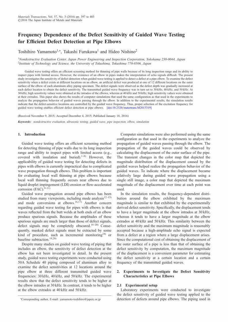
the experiments was made of aluminum alloy and comprisedtwo straight pipes connected at an elbow, as shown in Fig. 1.The pipes were 50A Schedule 40 (outer diameter of 60.5mmand wall thickness of 3.9mm). The elbow was a long radiuselbow that complied with JIS B2313 (comparable to ASMEB16.9). Each end of the elbow was welded to one of thestraight pipes.
The dry-coupled piezoelectric ring-shaped sensor systempresented in previous studies17,18) was used to transmit andreceive guided waves in the experiments. The sensor systemcomprised two sets of eight transducer elements aligned suchthat they were placed at equal intervals around the outersurface of the pipe. These transducer elements were orientedso that they would vibrate in the circumferential direction ofthe pipe to preferentially transmit and receive fundamentaltorsional-mode T(0, 1) guided waves. One set of the eighttransducer elements was used as a transmitter, while the otherset was used as a receiver. The transmitter was placed485mm before the inlet of the elbow and the receiver wasplaced 30mm before the transmitter, as shown in Fig. 1.
Hanning window-modulated six-cycle sinusoidal toneburst signals were generated by a function generator(Tektronix AFG3102), amplified to 120V peak-to-peak bya bipolar amplifier (NF BA4825), and fed into the transmitter.A programmable filter (NF 3628) was employed to yield25-fold signal amplification and to allow signals within the«10 kHz bandwidth around a given center frequency topass through. The resulting signals were observed andcaptured by a digital oscilloscope (Tektronix DPO7054).Every 100 consecutive waveform samples were averagedin the oscilloscope to improve the signal-to-noise ratio(S/N).
To determine the observed signal variations according tothe elbow defect location, 12 piping specimens of the sameconfiguration were prepared, as shown in Fig. 1. For eachspecimen, a single defect was made at one of the 12 locationspresented in Fig. 2. Figure 3 shows the carbide cutting toolused to make these defects on the outer surface of the pipewall. The diameter of the carbide cutting bit was 9.5mm. Thedepth of each defect was gradually increased in 0.25mmincrements up to 2.0mm. The observed signals were storedfor each step of the defect depth on the 12 piping specimens.
Three frequencies (30 kHz, 40 kHz, and 50 kHz) wereapplied as the center frequency of the excitation signal forthe transmitter to determine how the characteristics of theobserved signals changed according to the frequency of theguided waves.
2.2 Observations of defect signalsFigure 4 shows a typical waveform obtained from the
measurements before a defect was made at the elbow. Signal① is that of the guided waves propagating directly from thetransmitter to the receiver. Signal ② is formed from severalwave packets reflected around the elbow. This group of wavepackets mainly comprises the two wave packets reflectedfrom the two butt welds at the ends of the elbow. Signal ③arises from the waves reflected by the lower right end of thepiping specimen shown in Fig. 1.
485
120
2485
Receiver Transmitter
1000
Welds
30
60.5
3.9
(unit: mm)
Fig. 1 Schematic of the piping specimen with a piezoelectric ring-shapedsensor system.
10˚
10˚
35˚
35˚
20 mm
Sensor side
Fig. 2 Twelve locations at which artificial defects were made in elbows.
Fig. 3 Photograph of artificial defect and carbide cutting bit used to makeit.
Fig. 4 Typical waveform for a pipe without defect; ①: wave packetpropagating directly from transmitter to receiver,②: several wave packetsreflected around the elbow, ③: wave packet reflected by the lower end ofthe piping specimen.
T. Yamamoto, T. Furukawa and H. Nishino398
In general, the amplitude of a signal caused by a defect ismuch less than that of the spurious signal ② (approximately10% or less). In addition, the waveform of signal ② isdifferent for each specimen because of the irreproducibility ofwelds between specimens.1820) Since spurious signals suchas signal ② disturb or even obscure defect signals, signalprocessing is necessary to extract the signal difference due tothe defect. To solve this problem, incremental monitoringwas suggested in Ref. 18) and the effectiveness of thebaseline subtraction was studied in Ref. 19) and 20).
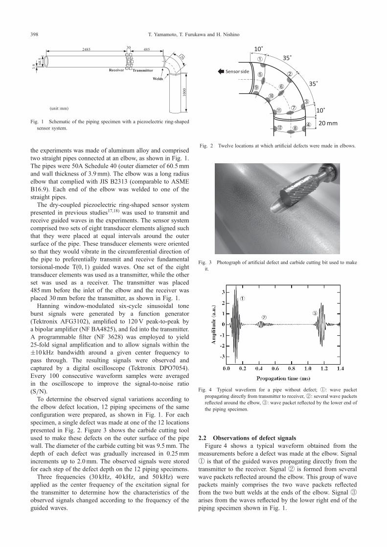
Figure 5 shows the waveforms of the observed signalswith increasing defect depth when the frequency of theexcitation signal was set to 50 kHz. The waveforms inFigs. 5(a), 5(b), and 5(c) were obtained when the defect wasmade at locations①,②, and④, respectively; these locationsare stipulated in Fig. 2. To focus on the signal variations withdefect depth, only the range from 350 µs to 600 µs isdisplayed. In these graphs, the signal amplitudes arenormalized such that the amplitude of the signal that
corresponds to signal ① in Fig. 4 is unity for eachmeasurement condition. The normalized amplitudes areexpressed in per mil (‰). Two overlapping wave packetscan be observed in these waveforms. The first one appearsnear 400450 µs, and the second one appears around 500550 µs. These two wave packets are mainly caused byreflections from the two welds at the ends of the elbow. Theamplitudes of these wave packets are different for each defectlocation (i.e., for each specimen) because of the differences inthe welds.
The signal variations due to the defect depth increaseappeared in the waveform at different times according to thedefect location. In Fig. 5, signal variations are observablearound 430 µs, 480 µs, and 540 µs for defect locations ①, ②,and ④, respectively. To clarify these signal variations, abaseline subtraction method was adopted. Figures 6(a), 6(b),and 6(c) show the signals obtained by subtracting thebaseline signal (the signal when the defect depth was 0mm)from the signals in Figs. 5(a), 5(b), and 5(c), respectively.
(a)
(b)
(c)
Fig. 5 Waveforms of observed signals for different defect depths at50 kHz; (a) defect at ①, (b) defect at ②, (c) defect at ④.
(a)
(b)
(c)
Fig. 6 Defect signal waveforms at 50 kHz obtained by subtracting thebaseline signal; (a) defect at ①, (b) defect at ②, (c) defect at ④.
Frequency Dependence of the Defect Sensitivity of Guided Wave Testing for Efficient Defect Detection at Pipe Elbows 399
Spurious signals were eliminated following subtraction, andthus, only the defect signals were extracted. For each defectlocation, the amplitude of the defect signal increases with thedefect depth.
2.3 Defect sensitivityTo quantify the increasing rate of the defect signal
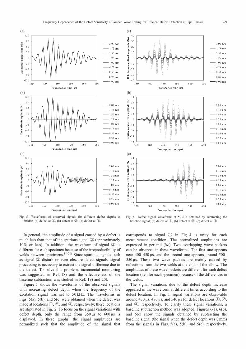
amplitude with respect to defect depth, Figs. 7(a), 7(b), and7(c) show the correlations between the cross-sectional losscaused by the defect and the maximum amplitude of thedefect signal for defect locations ①, ②, and ④, respectively.In the graphs, the cross-sectional loss is represented as theproportion (%) of the maximum cross-sectional area of thedefect to the cross-sectional area of the intact pipe wall. The
filled circles indicate the data obtained from the experiments,whereas the solid lines are the least-squares regression linesderived from the data. In this study, defect sensitivity isdefined as the slope of the least-squares regression line of thecorrelation between the cross-sectional loss and the max-imum amplitude of the defect signal at each defect location.
The measurements at the 12 piping specimens provide thedefect sensitivity values at the 12 locations indicated inFig. 2. Figure 8 shows the defect sensitivity values at these12 locations for three frequencies: 30 kHz, 40 kHz, and50 kHz. As shown in Fig. 8, the defect sensitivity depends onboth location and frequency. For 30 kHz, higher sensitivityvalues are derived from the elbow intrados, whereas for40 kHz and 50 kHz, higher sensitivity values are derived fromthe elbow extrados. In Fig. 9, the sensitivity values arenormalized such that the defect sensitivity at a straight part ofthe piping is unity. The defect sensitivity at a straight part ofthe piping was obtained for each frequency with a 50ASchedule 40 straight pipe of aluminum alloy in the samemanner as in the experiments to obtain the sensitivity at theelbow. The obtained defect sensitivities at the straight partof the piping are 4.96‰/%, 4.76‰/%, and 6.79‰/% for30 kHz, 40 kHz, and 50 kHz, respectively.
As shown in Fig. 9, at several locations around the elbow,the defect sensitivity is close to one, which is the defectsensitivity of the straight part of the piping. Furthermore,these sensitive locations differ depending on the guided wavefrequency. For example, the defect sensitivity is nearly one atthe elbow intrados for 30 kHz and at the elbow extrados for50 kHz. This characteristic implies that appropriate frequencyselection enables defect detection in the intended area of anelbow with the same sensitivity as that in a straight part of thepiping. This frequency-dependent behavior of guided wavesoffers great potential for high-sensitivity defect detection byguided wave testing at pipe elbows.
(a)
0
5
10
15
20
25
30
35
0 1 2 3 4
Rel
ativ
e no
rmal
ized
am
plitu
de (‰
)
Cross-sectional loss (%)
experimental value
least squares regression line
Sensitivity7.4 ‰/%
(b)
0
5
10
15
20
25
30
35
40
0 1 2 3 4
Rel
ativ
e no
rmal
ized
am
plitu
de (‰
)
Cross-sectional loss (%)
experimental value
least squares regression line
Sensitivity7.9 ‰/%
(c)
0
5
10
15
20
25
30
35
0 1 2 3 4
Rel
ativ
e no
rmal
ized
am
plitu
de (‰
)
Cross-sectional loss (%)
experimental value
least squares regression line
Sensitivity7.1 ‰/%
Fig. 7 Correlations between cross-sectional loss caused by defect andmaximum amplitude of defect signal at 50 kHz; (a) defect at①, (b) defectat ②, (c) defect at ④.
30 kHz
Sens
or s
ide
2.8
4.1
1.4
40 kHz
Sens
or s
ide
2.8
3.9
4.2
50 kHz
Sens
or s
ide
5.6
4.2
7.1
Fig. 8 Defect sensitivity (‰/%) at 12 locations at 30 kHz, 40 kHz, and50 kHz.
30 kHzSe
nsor
sid
e
0.6
0.8
0.3
40 kHz
Sens
or s
ide
0.6
0.8
0.9
50 kHz
Sens
or s
ide
0.8
0.6
1.0
Fig. 9 Normalized defect sensitivity at 12 locations at 30 kHz, 40 kHz, and50 kHz.
T. Yamamoto, T. Furukawa and H. Nishino400
3. FEM Simulations to Investigate Characteristics ofGuided Wave Propagation at Pipe Elbows
3.1 Configuration of FEM simulationsIn the preceding section, the presented experimental results
demonstrated that the defect sensitivity depends on both thedefect location and the excitation signal frequency whenguided wave testing is applied to detect defects at pipeelbows. This section shows the results of computersimulations conducted to determine the mechanism of thisphenomenon. To conduct these simulations, the commercialsimulation software ComWAVE was used.
ComWAVE, developed by ITOCHU Techno-SolutionsCorporation, is ultrasonic simulation software that performsmodeling, mesh generation, numerical computation, andvisualization of the results.21) ComWAVE employs finiteelement method (FEM) and performs computations using afinite element model developed with identical cubic elements(voxel elements). Creating a model with identical cubicelements simplifies the matrix formulation of FEM andsignificantly reduces computation time and memory. Thetime derivative of the equation to be solved is discretized by asecond-order central difference scheme. Subsequently, theequation is solved explicitly.
Our group has been performing guided wave testingsimulations using ComWAVE. A previous study22) validatedthe use of ComWAVE for simulations of guided wavespropagating along piping by comparing the simulation resultswith theoretical and experimental results. This study alsoshowed the influence of a pipe elbow on guided wavepropagation. In an experimental study,17) the mode con-versions of guided waves from the fundamental torsionalmode T(0, 1) to the torsional modes T(1, 1), T(2, 1), T(3, 1),and T(4, 1) were investigated at the elbow of a pipingspecimen. Ring-shaped sensor systems, such as that shown in2.1, were placed before and after the elbow and used as atransmitter and receiver, respectively. Signals received fromthe eight transducer elements of the receiver were used toobserve the mode conversions due to the elbow. The firstnumber of each mode notation, including T(1, 1), indicatesthe harmonic order of the vibration displacement in thecircumferential direction of the pipe. The displacementdirection is reversed at certain intervals along the circum-ference, and these intervals change according to the harmonicorder. Subsequently, each guided wave mode was traced byanalyzing the signal differences among the positions of theeight transducer elements aligned along the circumference. InRef. 22), simulations applying the same configuration as thatused in these experiments were conducted. In the simulations,the circumferential components of the displacements at thepositions of the eight transducer elements were observed.The simulation results showed the same mode conversionphenomena as those observed in the experiments. In thepresent study, the same simulation procedure was used.
To conduct the simulations with the same configuration asthat used in the experiments described in the precedingsection, the shape of the specimens used in the experimentswas reconstructed by combining basic geometric shapes forthe simulation model. The two straight parts of the pipingwere modeled as hollow cylinders, and the elbow was
modeled as a quarter of a hollow torus. The weld beads atboth ends of the elbow cause guided wave reflection, but theywere omitted in the simulation model because they did notsignificantly affect the analysis results shown later inSec. 3.2.
The specimens were made of aluminum alloy. Thevelocities of longitudinal and shear waves in the pipe wallwere set to 6,400m/s and 3,120m/s, respectively. Thedensity of aluminum alloy was set to 2,700 kg/m3. Thematerial properties were not defined in the regions other thanthe pipe walls. In ComWAVE, these undefined regions weretreated as perfect reflectors and computations were notperformed inside these regions to save computation time.
A transmitter was placed 485mm before the inlet of theelbow. This transmitter comprised eight vibrating blocksaligned at equal intervals in the circumferential directionof the outer surface of the pipe. All the blocks weresynchronously vibrated in the same circumferential directionto generate fundamental torsional mode T(0, 1) guidedwaves. The displacement of each transmitter element duringeach time step comprised the excitation signal. The excitationsignal was a Hanning window-modulated six-cycle sinus-oidal tone-burst signal with a certain center frequency. Sincethe aim of the simulation was to observe how guided wavespropagate through an elbow, the receiver was omitted in thesimulation model.
The whole simulation model was built with 0.5mm voxels.Approximately 2 h were needed to perform the simulation foreach condition via parallel computation on four processingcores of a computer with two Intel Xeon X5660 processors(2.8GHz, six cores for each) and 32GB of main memory.
3.2 Simulation resultsBecause ComWAVE calculates the output parameters
during each time step, it can display the propagation ofultrasonic waves as transient changes in the magnitudedistribution of the particle displacement caused by ultrasonicwaves.
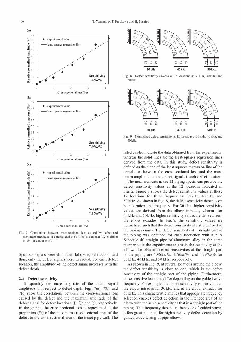
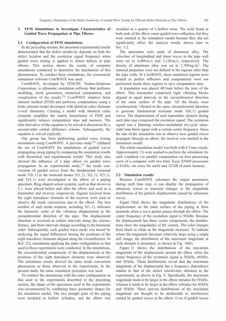
Figure 10(a) shows the magnitude distributions of thedisplacement on the outer surface of the piping at threemoments when a wave packet passes through the elbow. Thecenter frequency of the excitation signal is 50 kHz. Becausethe displacement has three vector components, the distribu-tions show the magnitudes of the vectors. The color changesfrom black to white as the magnitude increases. To indicatewhere the magnitude becomes relatively large using a singlestill image, the distribution of the maximum magnitude ateach element is presented, as shown in Fig. 10(b).
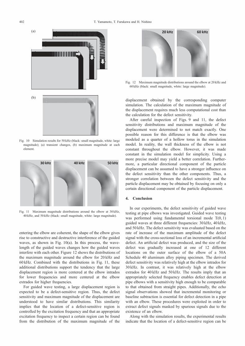
Figure 11 shows the distributions of the maximummagnitude of the displacement around the elbow when thecenter frequency of the excitation signal is 30 kHz, 40 kHz,and 50 kHz. These distributions reveal that the maximummagnitude of the displacement has a frequency dependencesimilar to that of the defect sensitivities obtained in theexperiments, as shown in Fig. 9. Specifically, the maximummagnitude tends to be larger at the elbow intrados for 30 kHz,whereas it tends to be larger at the elbow extrados for 40 kHzand 50 kHz. These uneven distributions of the maximummagnitude are thought to be attributable to interferencecaused by guided waves at the elbow. Even if guided waves
Frequency Dependence of the Defect Sensitivity of Guided Wave Testing for Efficient Defect Detection at Pipe Elbows 401
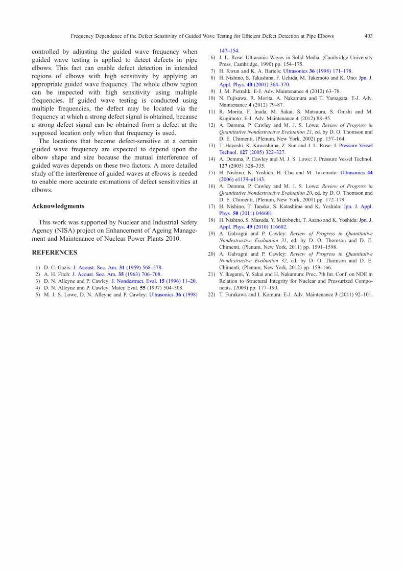
entering the elbow are coherent, the shape of the elbow givesrise to constructive and destructive interference of the guidedwaves, as shown in Fig. 10(a). In this process, the wave-length of the guided waves changes how the guided wavesinterfere with each other. Figure 12 shows the distributions ofthe maximum magnitude around the elbow for 20 kHz and60 kHz. Combined with the distributions in Fig. 11, theseadditional distributions support the tendency that the largedisplacement region is more centered at the elbow intradosfor lower frequencies and more centered at the elbowextrados for higher frequencies.
For guided wave testing, a large displacement region isexpected to be a defect-sensitive region. Thus, the defectsensitivity and maximum magnitude of the displacement areunderstood to have similar distributions. This similarityimplies that the location of a defect-sensitive region iscontrolled by the excitation frequency and that an appropriateexcitation frequency to inspect a certain region can be foundfrom the distribution of the maximum magnitude of the
displacement obtained by the corresponding computersimulation. The calculation of the maximum magnitude ofthe displacement requires much less computational cost thanthe calculation for the defect sensitivity.
After careful inspection of Figs. 9 and 11, the defectsensitivity distributions and maximum magnitude of thedisplacement were determined to not match exactly. Onepossible reason for this difference is that the elbow wasmodeled as a quarter of a hollow torus in the simulationmodel. In reality, the wall thickness of the elbow is notconstant throughout the elbow. However, it was madeconstant in the simulation model for simplicity. Using amore precise model may yield a better correlation. Further-more, a particular directional component of the particledisplacement can be assumed to have a stronger influence onthe defect sensitivity than the other components. Thus, astronger correlation between the defect sensitivity and theparticle displacement may be obtained by focusing on only acertain directional component of the particle displacement.
4. Conclusion
In our experiments, the defect sensitivity of guided wavetesting at pipe elbows was investigated. Guided wave testingwas performed using fundamental torsional mode T(0, 1)guided waves at three different frequencies: 30 kHz, 40 kHz,and 50 kHz. The defect sensitivity was evaluated based on therate of increase of the maximum amplitude of the defectsignal with the cross-sectional loss of an incremental artificialdefect. An artificial defect was produced, and the size of thedefect was gradually increased at one of 12 differentlocations on the outer surface of the elbow of a 50ASchedule 40 aluminum alloy piping specimen. The deriveddefect sensitivity was relatively high at the elbow intrados for30 kHz. In contrast, it was relatively high at the elbowextrados for 40 kHz and 50 kHz. The results imply that anappropriately selected frequency enables defect detection atpipe elbows with a sensitivity high enough to be comparableto that obtained from straight pipes. Additionally, the echosignal observations showed that incremental monitoring orbaseline subtraction is essential for defect detection in a pipewith an elbow. These procedures were exploited in order toextract defect signals masked by spurious signals due to theexistence of an elbow.
Along with the simulation results, the experimental resultsindicate that the location of a defect-sensitive region can be
(a)
(b)
Fig. 10 Simulation results for 50 kHz (black: small magnitude, white: largemagnitude); (a) transient changes, (b) maximum magnitude at eachelement.
30 kHz 40 kHz 50 kHz
Fig. 11 Maximum magnitude distributions around the elbow at 30 kHz,40 kHz, and 50 kHz (black: small magnitude, white: large magnitude).
20 kHz 60 kHz
Fig. 12 Maximum magnitude distributions around the elbow at 20 kHz and60 kHz (black: small magnitude, white: large magnitude).
T. Yamamoto, T. Furukawa and H. Nishino402
controlled by adjusting the guided wave frequency whenguided wave testing is applied to detect defects in pipeelbows. This fact can enable defect detection in intendedregions of elbows with high sensitivity by applying anappropriate guided wave frequency. The whole elbow regioncan be inspected with high sensitivity using multiplefrequencies. If guided wave testing is conducted usingmultiple frequencies, the defect may be located via thefrequency at which a strong defect signal is obtained, becausea strong defect signal can be obtained from a defect at thesupposed location only when that frequency is used.
The locations that become defect-sensitive at a certainguided wave frequency are expected to depend upon theelbow shape and size because the mutual interference ofguided waves depends on these two factors. A more detailedstudy of the interference of guided waves at elbows is neededto enable more accurate estimations of defect sensitivities atelbows.
Acknowledgments
This work was supported by Nuclear and Industrial SafetyAgency (NISA) project on Enhancement of Ageing Manage-ment and Maintenance of Nuclear Power Plants 2010.
REFERENCES
1) D. C. Gazis: J. Acoust. Soc. Am. 31 (1959) 568578.2) A. H. Fitch: J. Acoust. Soc. Am. 35 (1963) 706708.3) D. N. Alleyne and P. Cawley: J. Nondestruct. Eval. 15 (1996) 1120.4) D. N. Alleyne and P. Cawley: Mater. Eval. 55 (1997) 504508.5) M. J. S. Lowe, D. N. Alleyne and P. Cawley: Ultrasonics 36 (1998)
147154.6) J. L. Rose: Ultrasonic Waves in Solid Media, (Cambridge University
Press, Cambridge, 1990) pp. 154175.7) H. Kwun and K. A. Bartels: Ultrasonics 36 (1998) 171178.8) H. Nishino, S. Takashina, F. Uchida, M. Takemoto and K. Ono: Jpn. J.
Appl. Phys. 40 (2001) 364370.9) J. M. Pietralik: E-J. Adv. Maintenance 4 (2012) 6378.10) N. Fujisawa, R. Morita, A. Nakamura and T. Yamagata: E-J. Adv.
Maintenance 4 (2012) 7987.11) R. Morita, F. Inada, M. Sakai, S. Matsuura, S. Onishi and M.
Kugimoto: E-J. Adv. Maintenance 4 (2012) 8895.12) A. Demma, P. Cawley and M. J. S. Lowe: Review of Progress in
Quantitative Nondestructive Evaluation 21, ed. by D. O. Thomson andD. E. Chimenti, (Plenum, New York, 2002) pp. 157164.
13) T. Hayashi, K. Kawashima, Z. Sun and J. L. Rose: J. Pressure VesselTechnol. 127 (2005) 322327.
14) A. Demma, P. Cawley and M. J. S. Lowe: J. Pressure Vessel Technol.127 (2005) 328335.
15) H. Nishino, K. Yoshida, H. Cho and M. Takemoto: Ultrasonics 44(2006) e1139e1143.
16) A. Demma, P. Cawley and M. J. S. Lowe: Review of Progress inQuantitative Nondestructive Evaluation 20, ed. by D. O. Thomson andD. E. Chimenti, (Plenum, New York, 2001) pp. 172179.
17) H. Nishino, T. Tanaka, S. Katashima and K. Yoshida: Jpn. J. Appl.Phys. 50 (2011) 046601.
18) H. Nishino, S. Masuda, Y. Mizobuchi, T. Asano and K. Yoshida: Jpn. J.Appl. Phys. 49 (2010) 116602.
19) A. Galvagni and P. Cawley: Review of Progress in QuantitativeNondestructive Evaluation 31, ed. by D. O. Thomson and D. E.Chimenti, (Plenum, New York, 2011) pp. 15911598.
20) A. Galvagni and P. Cawley: Review of Progress in QuantitativeNondestructive Evaluation 32, ed. by D. O. Thomson and D. E.Chimenti, (Plenum, New York, 2012) pp. 159166.
21) Y. Ikegami, Y. Sakai and H. Nakamura: Proc. 7th Int. Conf. on NDE inRelation to Structural Integrity for Nuclear and Pressurized Compo-nents, (2009) pp. 177190.
22) T. Furukawa and I. Komura: E-J. Adv. Maintenance 3 (2011) 92101.
Frequency Dependence of the Defect Sensitivity of Guided Wave Testing for Efficient Defect Detection at Pipe Elbows 403