Frequency and Severity of Belgian Road Traffic Accidents Studied by State Space Methods€¦ · · 2011-11-25The methodology used throughout the analysis is state space methods

Hermans, Wets and Van den Bossche 1

Frequency and Severity of Belgian Road Traffic Accidents Studied by State Space Methods

Elke Hermans, Geert Wets * and Filip Van den Bossche Transportation Research Institute Hasselt University, Campus Diepenbeek Agoralaan, Building D 3590 Diepenbeek, Belgium Tel: +32(0)11 26 87 05 Fax: +32(0)11 26 87 00 E-mail: [email protected]

* corresponding author


ABSTRACT In this paper we investigate the monthly frequency and severity of road traffic accidents in Belgium from 1974 to 1999. We describe the trend in the time series, quantify the impact of explanatory variables and make predictions. Laws concerning seat belts, speed and alcohol have proven successful. Furthermore, frost enhances road safety while sun has the opposite effect. Precipitation and thunderstorm particularly influence accidents with light injuries. Economic conditions have a limited impact. The methodology used throughout the analysis is state space methods. The results of this study are compared to those of an earlier research applying a regression model with autoregressive moving average errors on the same data. A lot of similarities between these two approaches were found. Keywords: road safety, time series, trend, seasonal, explanatory model, state space methodology, prediction.


1 INTRODUCTION Every year, Belgium has more or less 70.000 road casualties (BIVV 2001). During the past decennia there has been a steady increase in traffic volume, which resulted in continuously increasing traffic problems. This matter has such an impact on our society that the interest and need for an adequate road safety policy grows. In order to increase the level of road safety in the long term and to be able to take appropriate actions, we need to understand the underlying processes and their causes. Extensive and reliable data over a long period of time together with modelling techniques that are suitable for describing, interpreting and forecasting safety developments are required (EC 2004, 7). We will study the developments in the frequency and severity of road traffic accidents in Belgium over a relatively long period of time (1974-1999). Data in economics, engineering and medicine even as in road safety are often collected in the form of time series, that is a sequence of observations taken at regular intervals of time (Peña, Tiao and Stay 2001, 1). From the broad category of time series model construction methods we have applied state space methods in this study. This methodology will be explained in the remainder of the text, but one of the most important characteristics of state space time series models is that observations are regarded as being made up of distinct components such as trend, seasonal and regression elements, each of which is modelled separately (Durbin and Koopman 2001, vii) and have a direct interpretation. Furthermore, the components are allowed to change in time and the stationarity of the series is not required. The paper is organized as follows: first, a literature overview is given, followed by the presentation of the data. In section four the state space methodology is explained. In the fifth section the results are presented and discussed. Finally, a summary of the conclusions, topics for further research and a methodological appendix are provided. 2 TIME SERIES APPLICATIONS IN ROAD SAFETY The increasing interest in a traffic safe world is an incentive for the elaboration of numerous studies. These are very diverse in terms of problem description as well as data used. An important class of road safety models is based on time series analysis. The succession of data points in time is a fundamental aspect in this analysis. Models are used to describe the data behavior, to explain behavior of the time series in terms of exogenous variables and to forecast (Aoki 1987, v). The most relevant ideas of the developments in road safety inside this movement are described in the COST329 report of the European Commission (2004). In addition to giving a description of the trend in the traffic data, many models test the influence of explanatory factors. A simple, well-known example of such a time series model is the classical linear regression, which assumes a linear relationship between a criterion or dependent variable (yt) and one or more predictor or independent variables (xt). Explanatory models describe how the target variable depends on the explanatory variables and interventions. One special and prominent class of explanatory models in road safety analysis is known as the DRAG (Demand Routière, les Accidents et leur Gravité) family, extensively described in Gaudry and Lassarre (2000). DRAG models are structural explanatory models, including a relatively large number of explanatory


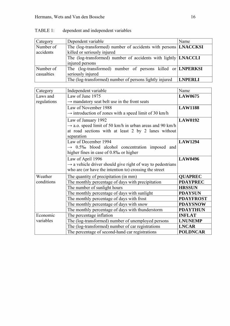
variables, whose partial effects on the exposure, the frequency and the severity of accidents are estimated by means of econometric methods (EC 2004, 174). The COST329 report (EC 2004, 47) mentions two main classes of univariate dynamic models: ARIMA models studied by Box and Jenkins and unobserved components models which are called structural models by Harvey. In a structural model each component or equation is intended to represent a specific feature or relationship in the system under study (Harvey and Durbin 1986, 188). The models used in this study, state space methods, belong to the latter group of models. To this day, Box-Jenkins methods for time series analysis are more widely applied and are more popular than state space methods but this study will show the strengths of the state space methodology. Both classes are concerned with the decomposition of an observed time series into a certain number of components. ARMA models decompose the series into an autoregressive process (AR), a moving average process (MA) and a random process. Unobserved components models decompose a series in a trend, a seasonal and an irregular part. An important characteristic is that the components can be stochastic. Moreover, explanatory variables can be added and intervention analysis carried out. The principal structural time series models are therefore nothing more than regression models in which the explanatory variables are functions of time and the parameters are time-varying (Harvey 1989, 10). The key to handling structural time series models is the state space form, with the state of the system representing the various unobserved components. Once in state space form, the Kalman filter (Kalman 1960) may be applied and this in turn leads to estimation, analysis and forecasting. In 1989, Harvey wrote a comprehensive book on structural time series models (primarily applied on economic time series) wherein a historical overview of the technique is given (Harvey, 22-23). In recent years, there has been a rapid growth of interest. Nowadays, the technique of unobserved components models is used in several studies: Flaig (2002) applied it to quarterly German GDP, Cuevas (2002) to real GDP and imports in Venezuela, Orlandi and Pichelmann (2000) to unemployment series. Beside those economic applications, this technique (more specifically an intervention analysis) was also used in traffic related research (Balkin and Ord 2001; Harvey and Durbin 1986). The state space methodology forms a well-used approach in modeling road accidents in a number of countries, for example the Netherlands (Bijleveld and Commandeur 2004), Sweden (Johansson 1996) and Denmark (Christens 2003). In this paper we will present the results of the first state space analysis on Belgian data. 3 DATA The data used in this study are monthly observations from January 1974 till December 1999. 12 observations each year, over a period of 26 years equals 312 observations. All data have been gathered from governmental ministries and official documents published by the Belgian National Institute for Statistics. In addition to four dependent traffic related variables, we study the effect of sixteen independent variables in this paper. These sixteen explanatory factors can be divided into three groups: juristic, climatologic and economic variables. Table 1 gives an overview of all the variables used in this study.


<INSERT TABLE 1: VARIABLES>

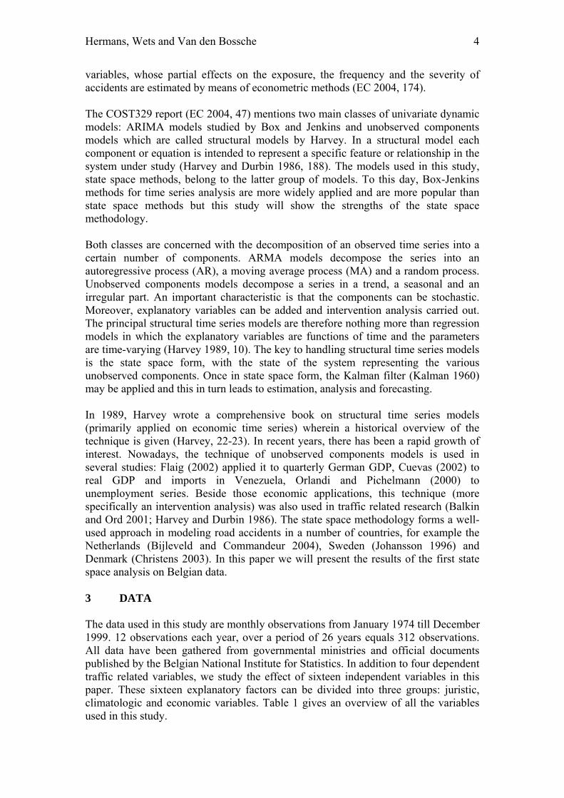
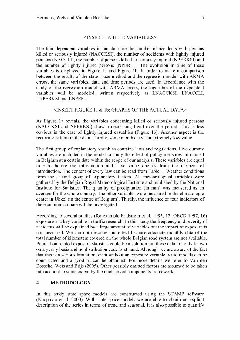
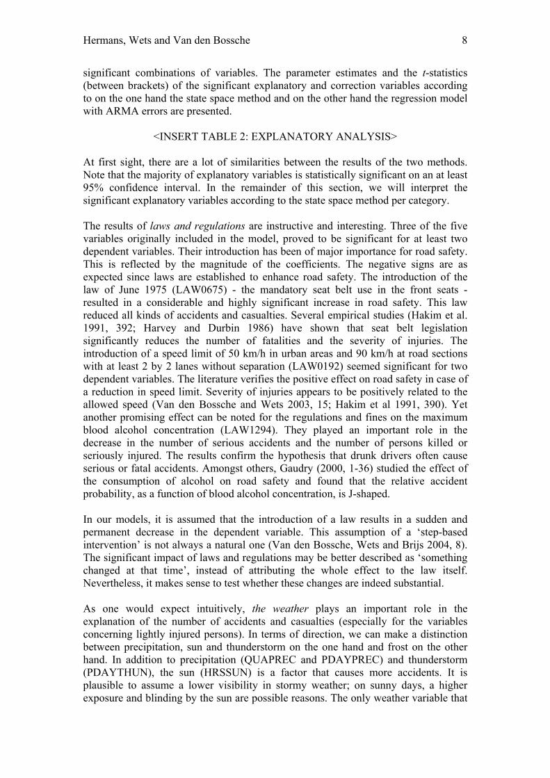
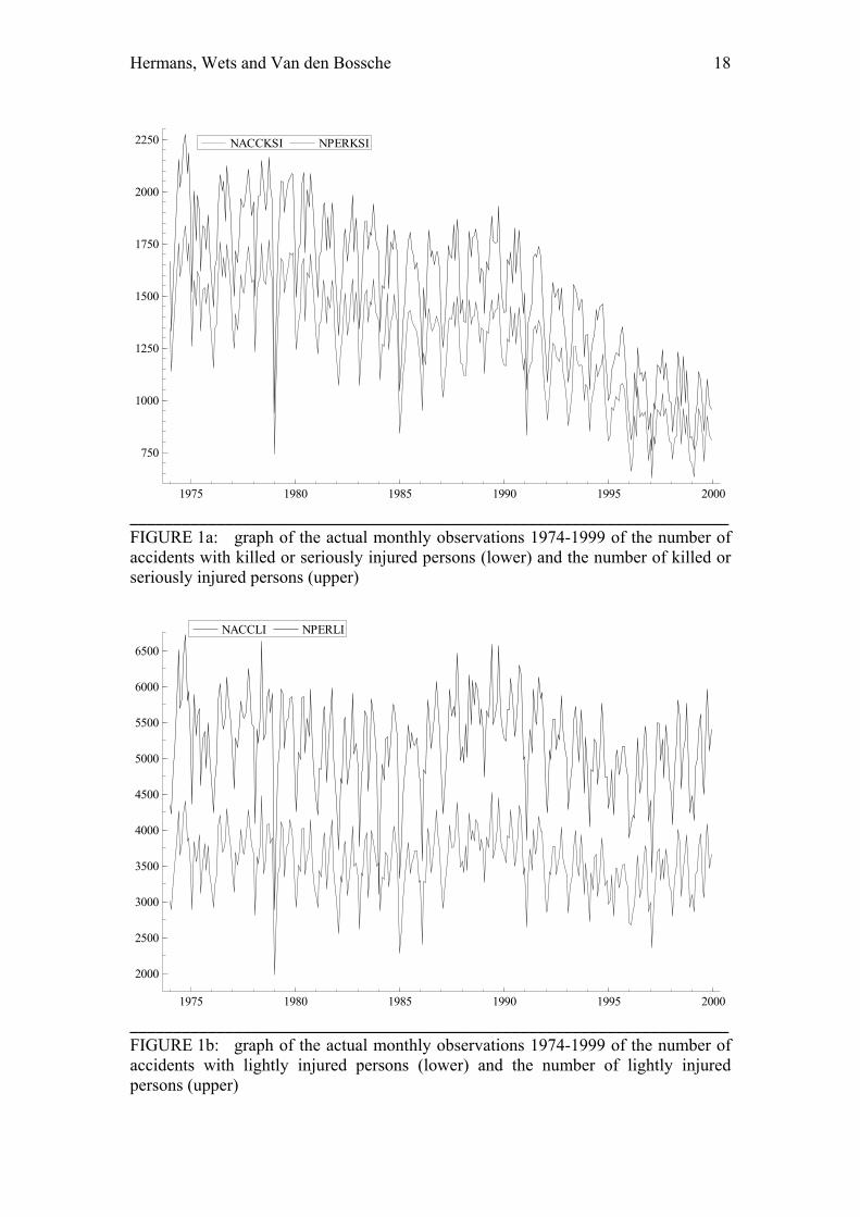
The four dependent variables in our data are the number of accidents with persons killed or seriously injured (NACCKSI), the number of accidents with lightly injured persons (NACCLI), the number of persons killed or seriously injured (NPERKSI) and the number of lightly injured persons (NPERLI). The evolution in time of these variables is displayed in Figure 1a and Figure 1b. In order to make a comparison between the results of the state space method and the regression model with ARMA errors, the same variables, data and time periods are used. In accordance with the study of the regression model with ARMA errors, the logarithm of the dependent variables will be modeled, written respectively as LNACCKSI, LNACCLI, LNPERKSI and LNPERLI.

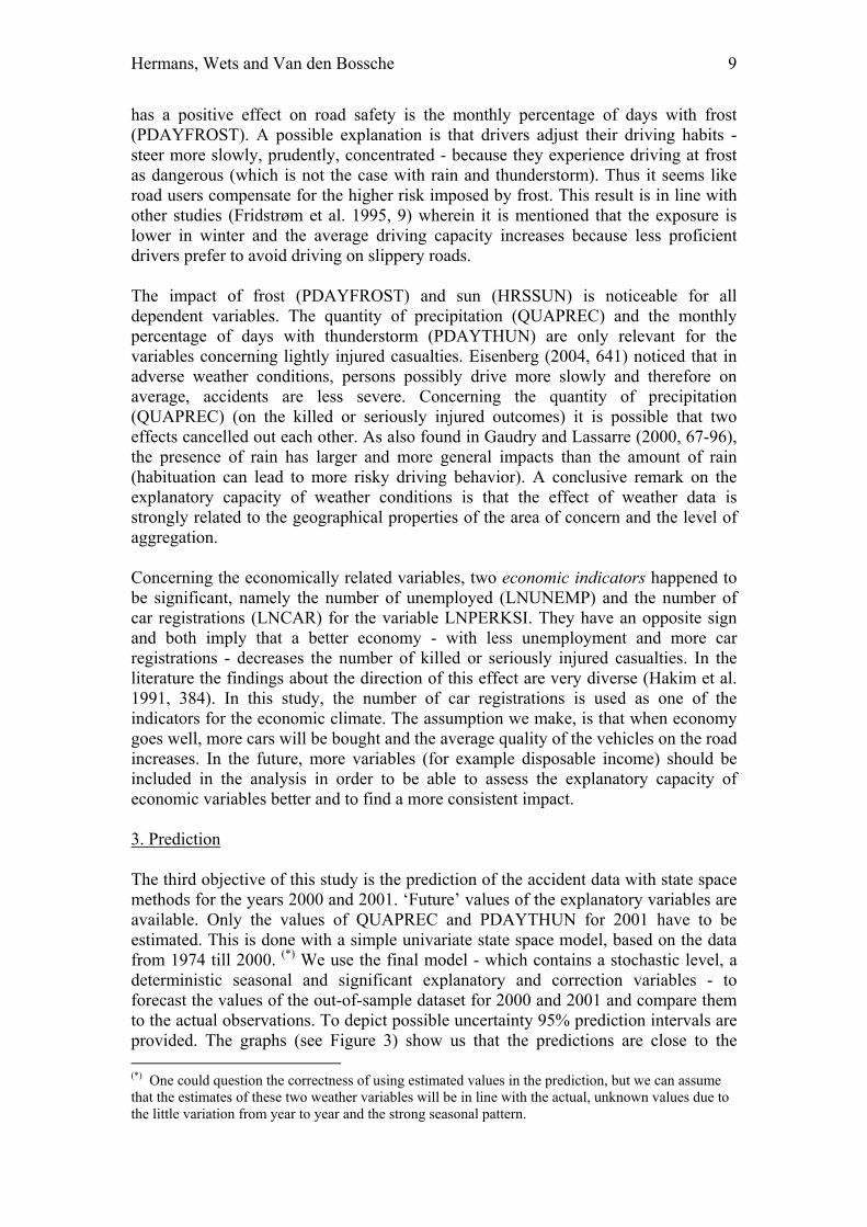
<INSERT FIGURE 1a & 1b: GRAPHS OF THE ACTUAL DATA> As Figure 1a reveals, the variables concerning killed or seriously injured persons (NACCKSI and NPERKSI) show a decreasing trend over the period. This is less obvious in the case of lightly injured casualties (Figure 1b). Another aspect is the recurring pattern in the data. Thirdly, some months have an extremely low value. The first group of explanatory variables contains laws and regulations. Five dummy variables are included in the model to study the effect of policy measures introduced in Belgium at a certain date within the scope of our analysis. These variables are equal to zero before the introduction and have value one as from the moment of introduction. The content of every law can be read from Table 1. Weather conditions form the second group of explanatory factors. All meteorological variables were gathered by the Belgian Royal Meteorological Institute and published by the National Institute for Statistics. The quantity of precipitation (in mm) was measured as an average for the whole country. The other variables were measured in the climatologic center in Ukkel (in the centre of Belgium). Thirdly, the influence of four indicators of the economic climate will be investigated. According to several studies (for example Fridstrøm et al. 1995, 12; OECD 1997, 16) exposure is a key variable in traffic research. In this study the frequency and severity of accidents will be explained by a large amount of variables but the impact of exposure is not measured. We can not describe this effect because adequate monthly data of the total number of kilometers covered on the whole Belgian road system are not available. Population related exposure statistics could be a solution but these data are only known on a yearly basis and no distribution code is at hand. Although we are aware of the fact that this is a serious limitation, even without an exposure variable, valid models can be constructed and a good fit can be obtained. For more details we refer to Van den Bossche, Wets and Brijs (2005). Other possibly omitted factors are assumed to be taken into account to some extent by the unobserved components framework. 4 METHODOLOGY In this study state space models are constructed using the STAMP software (Koopman et al. 2000). With state space models we are able to obtain an explicit description of the series in terms of trend and seasonal. It is also possible to quantify


the impact of explanatory factors. For example, the effect of road safety measures on the development in road safety over time can be checked by adding so-called intervention variables to the model. Apart from these purposes state space models can easily be used for forecasting. For a technical discussion of state space models we refer to the methodological appendix. The objective of our approach is to find the model that describes the data best. For each of the four dependent variables, we constructed several state space models, each with their specific components. To be able to choose the best model we use the Akaike Information Criterion (AIC), a measurement of fit that takes the number of parameters into account (Akaike 1973, 267-281; Koopman et al. 2000, 180). We conclude this section with the discussion of some of the advantages of state space models compared to classical regression. An interesting characteristic of state space methods is the possibility to model stochastically the variation in the estimation of the various components. Contrary to classical regression models, where components are fixed or unchangeable in time, a component can also vary in time. This is an advantage because variation in time makes it easier to follow the fluctuations in the data. Secondly, when the time dependency between observations is taken into account (which is not the case in classical regression analysis) the observation errors will mostly be situated more closely to independently random values. This makes significance tests of explanatory variables more reliable. Furthermore, state space methods can easily handle missing observations, multivariate data and (stochastic) explanatory variables. A last advantage is that the components can be modeled separately and interpreted directly. 5 RESULTS Not all numerical outcomes of the different models will be presented in this text. However, this section reports and discusses the most essential results of the analysis. It is divided into four parts. First, the outcomes of the descriptive analysis are presented, followed by an interpretation of the explanatory analysis. Next, the forecasting capacity is evaluated. Finally, we compare our results with those obtained by the regression model with ARMA errors and deduce the most important similarities and differences between these two methodologies. 1. Description Based on AIC we chose the model that describes the accident data best. For each of the four variables the same model resulted in the best fit. This contains a stochastic trend (that adapts every time period) and a deterministic or fixed recurring seasonal pattern. The interpretation of the seasonal coefficients shows that, concerning road safety, October and June are the most traffic unsafe months of the year. During these months, respectively approximately 13% and 11% more accidents happen than on average. The traffic insecurity in October can partly be explained by the fact that it is a long month (31 days) without holidays; it is autumn and there is the transition from Central European Summer Time to Central European Time; it is the start of the academic


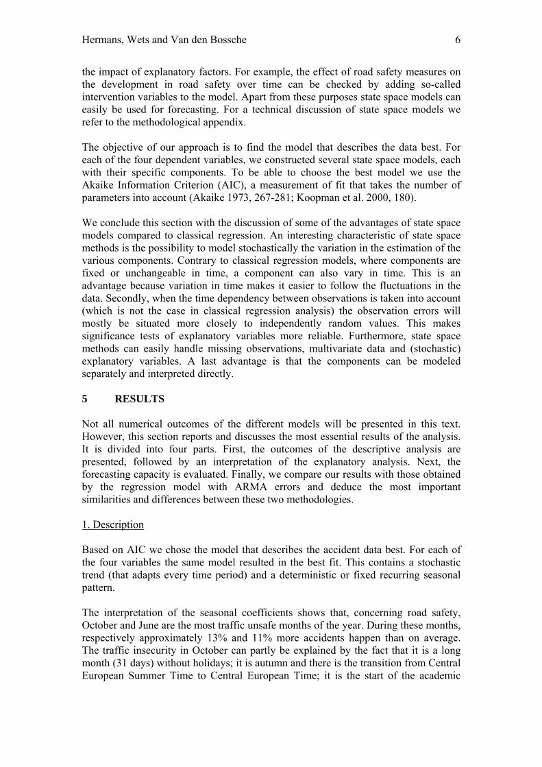
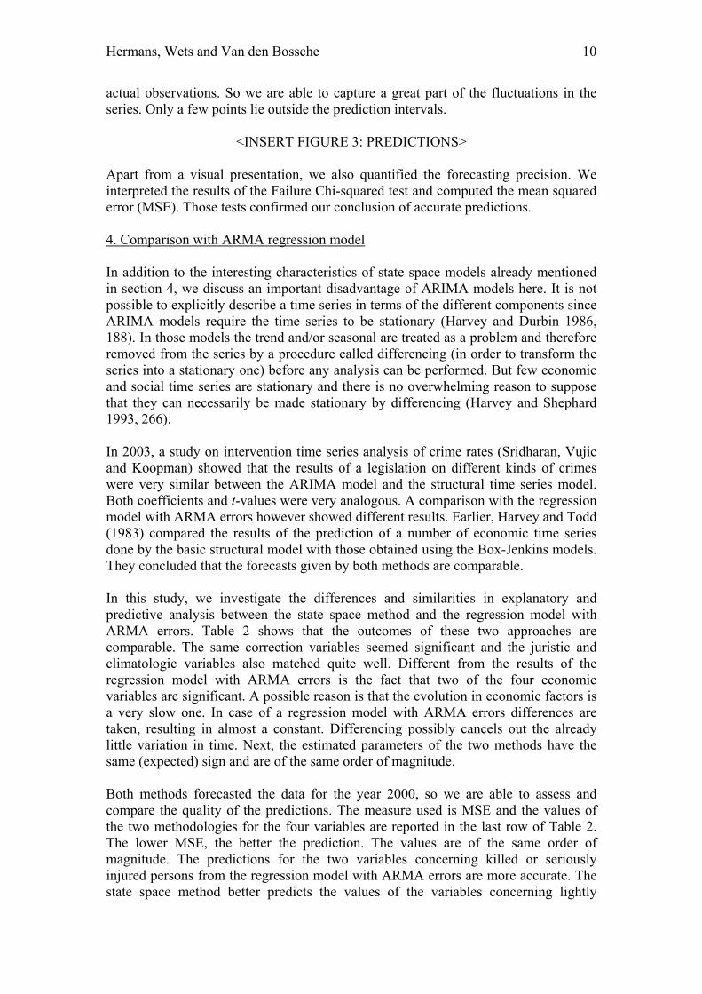
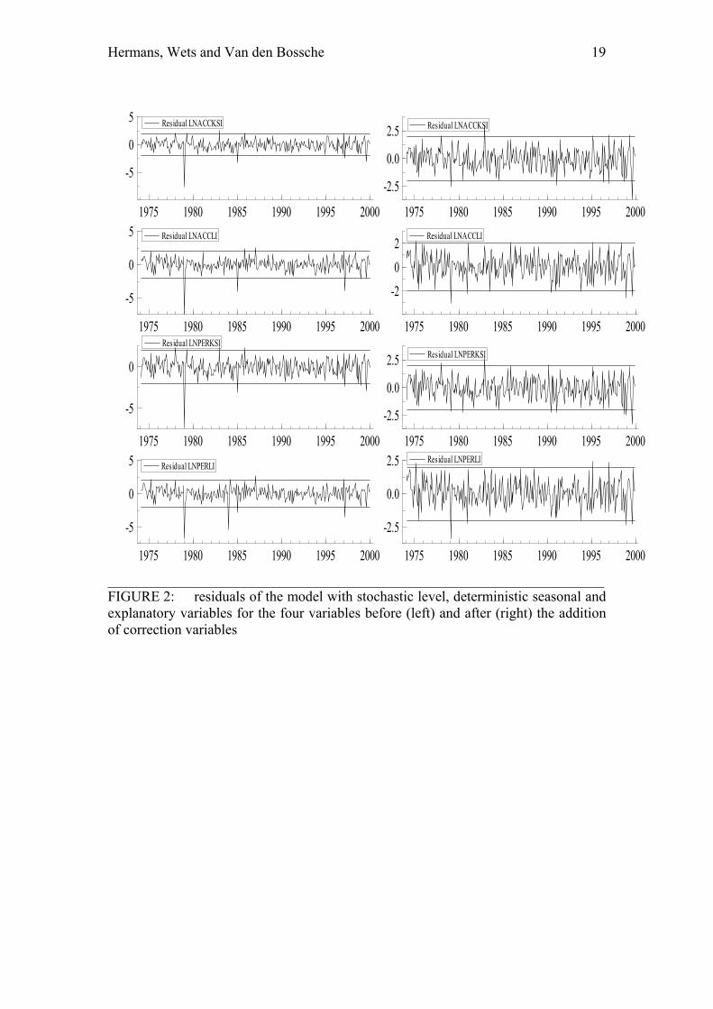
year; etc. Possible explanations for the large amount of accidents during June are not at hand. 2. Explanation When apart from the descriptive objective, the explanatory objective is aimed at, the effect of 16 independent variables is tested. In order to obtain (more) reliable results - which imply normally distributed residuals - we add correction variables to the model. The inclusion of correction variables has algebraically been presented in the model formulation (see the methodological appendix). In general, two main intervention effects can be distinguished (Sridharan, Vujic and Koopman 2003), namely a pulse intervention and a step intervention. The first effect is used to capture single special events since they may cause outlying observations which the pulse regression variable accounts for. The variable takes value 1 if t is the month that needs correction for a special event and has value 0 otherwise. The second intervention – called a step intervention or level shift – is introduced in the model to capture events such as the introduction of new policy measures. Laws and regulations can be incorporated in a model as this second type of intervention. Before its introduction the variable has value 0 while as from the moment of introduction it has value 1. Now, the focus is on the first type, the temporal pulse intervention. As could be seen on the graphs of the actual data (Figure 1a & 1b) as well as on the graph of the residuals (Figure 2), the number of accidents and casualties was unexpectedly low during some months. Either these months indeed had extremely low values, or some registration error was left in the accident statistics. We identify the extreme values for which correction is necessary.

<INSERT FIGURE 2: RESIDUALS> January 1979, January 1984 (only for LNPERLI, so probably a registration error occurred here), January 1985 and February 1997 are outliers. There are some indications for a very severe winter in 1979 and 1985 (BIVV 2001, 5). We explicitly correct for those four months by adding pulse intervention variables to the model, which are coded one during the month they represent and zero elsewhere. We are convinced that the most striking shocks must be excluded in order to fulfil the error terms conditions: no autocorrelation, homoscedasticity and normality. In the end, we want to obtain a correct parameter interpretation. The inclusion of these correction variables lowers the difference between the predicted and the real series and thus improves the quality of the estimations. All tested correction variables are highly statistically significant. The exact t-values are given in Table 2 under ‘Correction variables’. Taking these outliers into account, the fit of the models improves. The last step in the construction of the final model consists of the significance tests of the explanatory variables. An explanatory variable must have a significant influence on an at least 90% confidence level to be included in the final model. Each model was re-estimated after dropping the non-significant variables such that the ultimate model for every dependent variable consists of a stochastic level, a deterministic seasonal and significant correction and explanatory variables. The addition of significant explanatory variables further improves the fit. Table 2 gives an overview of all


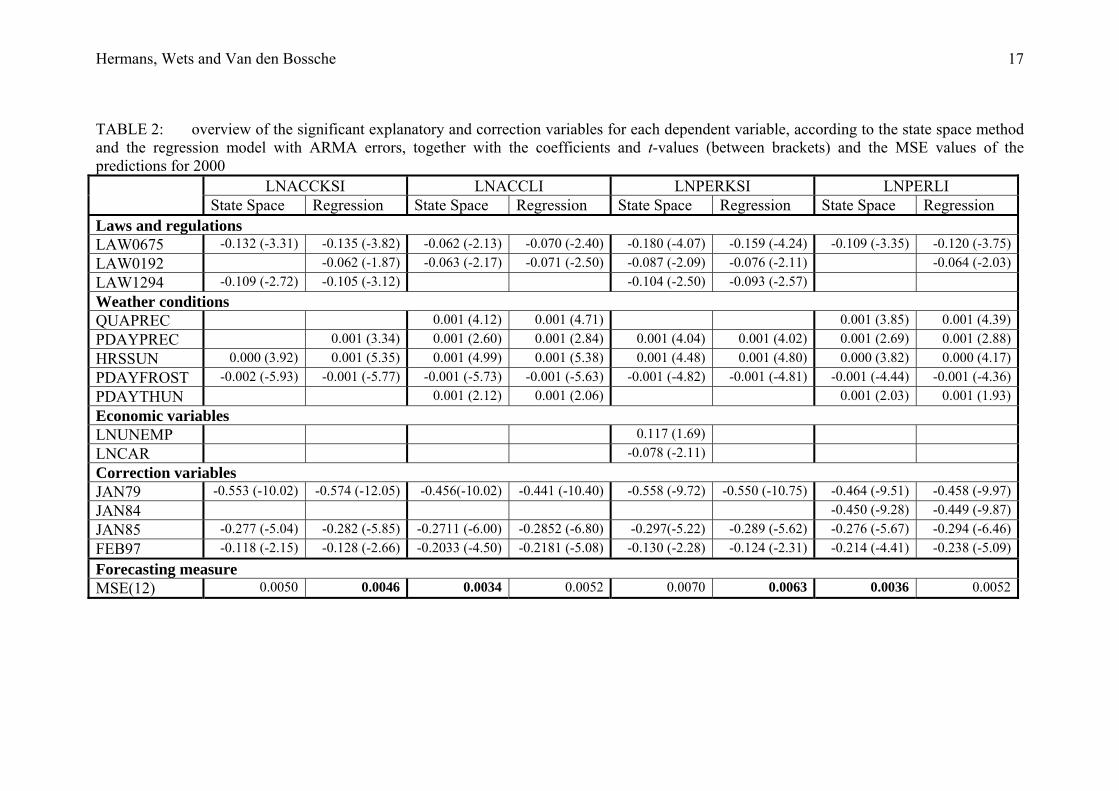
significant combinations of variables. The parameter estimates and the t-statistics (between brackets) of the significant explanatory and correction variables according to on the one hand the state space method and on the other hand the regression model with ARMA errors are presented.

<INSERT TABLE 2: EXPLANATORY ANALYSIS> At first sight, there are a lot of similarities between the results of the two methods. Note that the majority of explanatory variables is statistically significant on an at least 95% confidence interval. In the remainder of this section, we will interpret the significant explanatory variables according to the state space method per category. The results of laws and regulations are instructive and interesting. Three of the five variables originally included in the model, proved to be significant for at least two dependent variables. Their introduction has been of major importance for road safety. This is reflected by the magnitude of the coefficients. The negative signs are as expected since laws are established to enhance road safety. The introduction of the law of June 1975 (LAW0675) - the mandatory seat belt use in the front seats - resulted in a considerable and highly significant increase in road safety. This law reduced all kinds of accidents and casualties. Several empirical studies (Hakim et al. 1991, 392; Harvey and Durbin 1986) have shown that seat belt legislation significantly reduces the number of fatalities and the severity of injuries. The introduction of a speed limit of 50 km/h in urban areas and 90 km/h at road sections with at least 2 by 2 lanes without separation (LAW0192) seemed significant for two dependent variables. The literature verifies the positive effect on road safety in case of a reduction in speed limit. Severity of injuries appears to be positively related to the allowed speed (Van den Bossche and Wets 2003, 15; Hakim et al 1991, 390). Yet another promising effect can be noted for the regulations and fines on the maximum blood alcohol concentration (LAW1294). They played an important role in the decrease in the number of serious accidents and the number of persons killed or seriously injured. The results confirm the hypothesis that drunk drivers often cause serious or fatal accidents. Amongst others, Gaudry (2000, 1-36) studied the effect of the consumption of alcohol on road safety and found that the relative accident probability, as a function of blood alcohol concentration, is J-shaped. In our models, it is assumed that the introduction of a law results in a sudden and permanent decrease in the dependent variable. This assumption of a ‘step-based intervention’ is not always a natural one (Van den Bossche, Wets and Brijs 2004, 8). The significant impact of laws and regulations may be better described as ‘something changed at that time’, instead of attributing the whole effect to the law itself. Nevertheless, it makes sense to test whether these changes are indeed substantial. As one would expect intuitively, the weather plays an important role in the explanation of the number of accidents and casualties (especially for the variables concerning lightly injured persons). In terms of direction, we can make a distinction between precipitation, sun and thunderstorm on the one hand and frost on the other hand. In addition to precipitation (QUAPREC and PDAYPREC) and thunderstorm (PDAYTHUN), the sun (HRSSUN) is a factor that causes more accidents. It is plausible to assume a lower visibility in stormy weather; on sunny days, a higher exposure and blinding by the sun are possible reasons. The only weather variable that


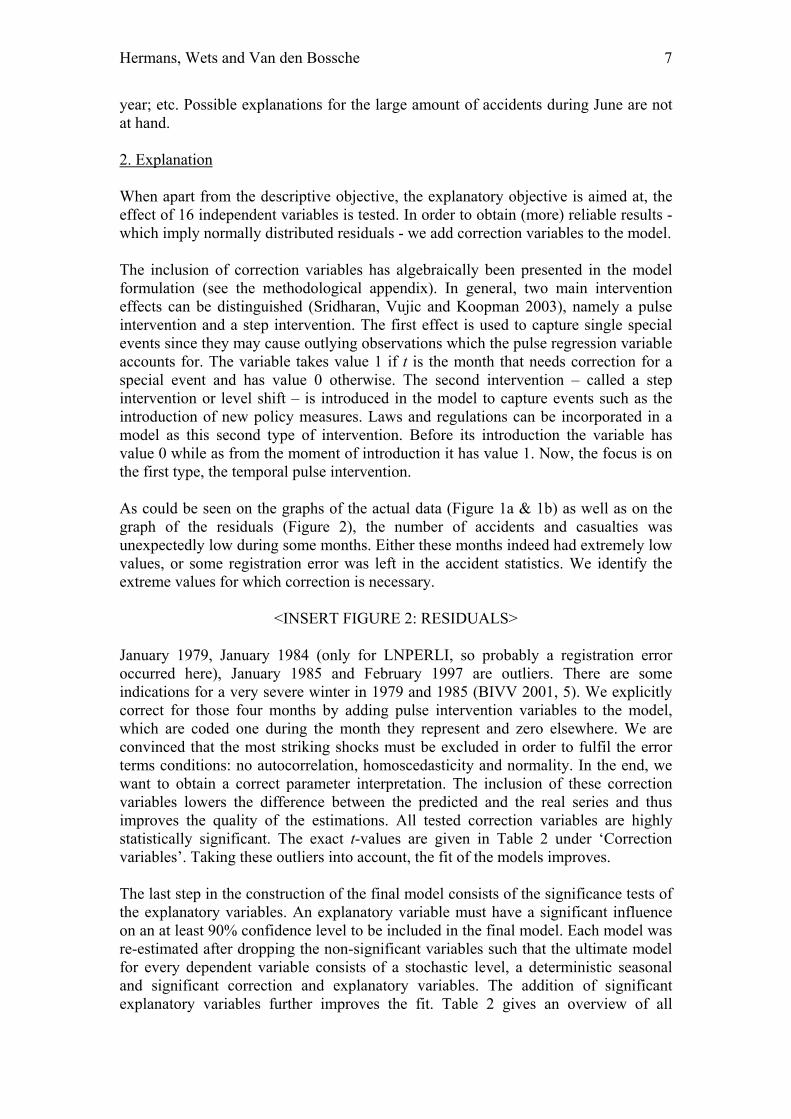
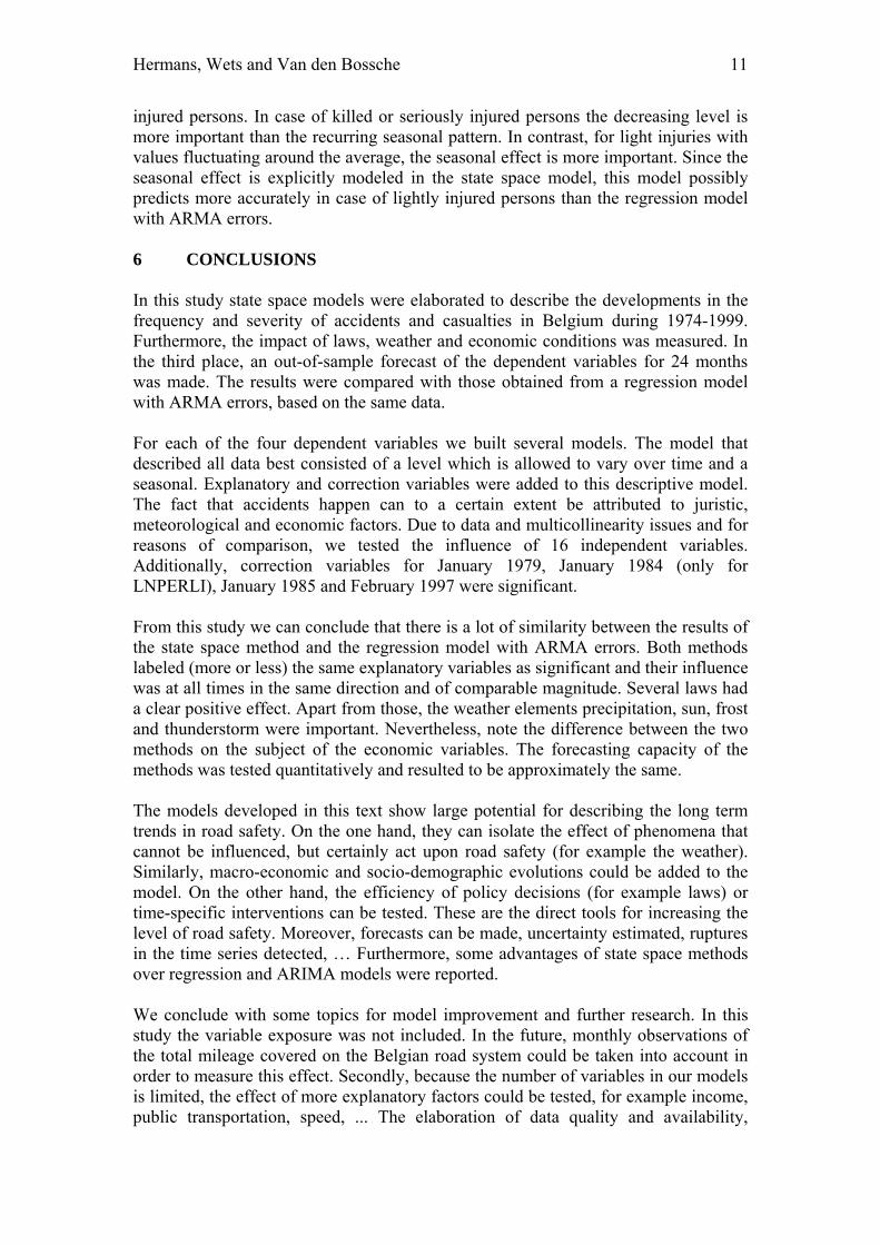
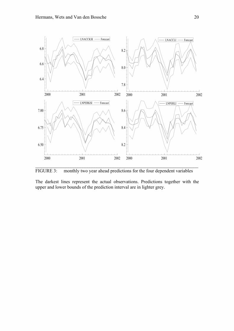
has a positive effect on road safety is the monthly percentage of days with frost (PDAYFROST). A possible explanation is that drivers adjust their driving habits - steer more slowly, prudently, concentrated - because they experience driving at frost as dangerous (which is not the case with rain and thunderstorm). Thus it seems like road users compensate for the higher risk imposed by frost. This result is in line with other studies (Fridstrøm et al. 1995, 9) wherein it is mentioned that the exposure is lower in winter and the average driving capacity increases because less proficient drivers prefer to avoid driving on slippery roads. The impact of frost (PDAYFROST) and sun (HRSSUN) is noticeable for all dependent variables. The quantity of precipitation (QUAPREC) and the monthly percentage of days with thunderstorm (PDAYTHUN) are only relevant for the variables concerning lightly injured casualties. Eisenberg (2004, 641) noticed that in adverse weather conditions, persons possibly drive more slowly and therefore on average, accidents are less severe. Concerning the quantity of precipitation (QUAPREC) (on the killed or seriously injured outcomes) it is possible that two effects cancelled out each other. As also found in Gaudry and Lassarre (2000, 67-96), the presence of rain has larger and more general impacts than the amount of rain (habituation can lead to more risky driving behavior). A conclusive remark on the explanatory capacity of weather conditions is that the effect of weather data is strongly related to the geographical properties of the area of concern and the level of aggregation. Concerning the economically related variables, two economic indicators happened to be significant, namely the number of unemployed (LNUNEMP) and the number of car registrations (LNCAR) for the variable LNPERKSI. They have an opposite sign and both imply that a better economy - with less unemployment and more car registrations - decreases the number of killed or seriously injured casualties. In the literature the findings about the direction of this effect are very diverse (Hakim et al. 1991, 384). In this study, the number of car registrations is used as one of the indicators for the economic climate. The assumption we make, is that when economy goes well, more cars will be bought and the average quality of the vehicles on the road increases. In the future, more variables (for example disposable income) should be included in the analysis in order to be able to assess the explanatory capacity of economic variables better and to find a more consistent impact. 3. Prediction The third objective of this study is the prediction of the accident data with state space methods for the years 2000 and 2001. ‘Future’ values of the explanatory variables are available. Only the values of QUAPREC and PDAYTHUN for 2001 have to be estimated. This is done with a simple univariate state space model, based on the data from 1974 till 2000. (*) We use the final model - which contains a stochastic level, a deterministic seasonal and significant explanatory and correction variables - to forecast the values of the out-of-sample dataset for 2000 and 2001 and compare them to the actual observations. To depict possible uncertainty 95% prediction intervals are provided. The graphs (see Figure 3) show us that the predictions are close to the (*) One could question the correctness of using estimated values in the prediction, but we can assume that the estimates of these two weather variables will be in line with the actual, unknown values due to the little variation from year to year and the strong seasonal pattern.


actual observations. So we are able to capture a great part of the fluctuations in the series. Only a few points lie outside the prediction intervals.

<INSERT FIGURE 3: PREDICTIONS> Apart from a visual presentation, we also quantified the forecasting precision. We interpreted the results of the Failure Chi-squared test and computed the mean squared error (MSE). Those tests confirmed our conclusion of accurate predictions. 4. Comparison with ARMA regression model In addition to the interesting characteristics of state space models already mentioned in section 4, we discuss an important disadvantage of ARIMA models here. It is not possible to explicitly describe a time series in terms of the different components since ARIMA models require the time series to be stationary (Harvey and Durbin 1986, 188). In those models the trend and/or seasonal are treated as a problem and therefore removed from the series by a procedure called differencing (in order to transform the series into a stationary one) before any analysis can be performed. But few economic and social time series are stationary and there is no overwhelming reason to suppose that they can necessarily be made stationary by differencing (Harvey and Shephard 1993, 266). In 2003, a study on intervention time series analysis of crime rates (Sridharan, Vujic and Koopman) showed that the results of a legislation on different kinds of crimes were very similar between the ARIMA model and the structural time series model. Both coefficients and t-values were very analogous. A comparison with the regression model with ARMA errors however showed different results. Earlier, Harvey and Todd (1983) compared the results of the prediction of a number of economic time series done by the basic structural model with those obtained using the Box-Jenkins models. They concluded that the forecasts given by both methods are comparable. In this study, we investigate the differences and similarities in explanatory and predictive analysis between the state space method and the regression model with ARMA errors. Table 2 shows that the outcomes of these two approaches are comparable. The same correction variables seemed significant and the juristic and climatologic variables also matched quite well. Different from the results of the regression model with ARMA errors is the fact that two of the four economic variables are significant. A possible reason is that the evolution in economic factors is a very slow one. In case of a regression model with ARMA errors differences are taken, resulting in almost a constant. Differencing possibly cancels out the already little variation in time. Next, the estimated parameters of the two methods have the same (expected) sign and are of the same order of magnitude. Both methods forecasted the data for the year 2000, so we are able to assess and compare the quality of the predictions. The measure used is MSE and the values of the two methodologies for the four variables are reported in the last row of Table 2. The lower MSE, the better the prediction. The values are of the same order of magnitude. The predictions for the two variables concerning killed or seriously injured persons from the regression model with ARMA errors are more accurate. The state space method better predicts the values of the variables concerning lightly


injured persons. In case of killed or seriously injured persons the decreasing level is more important than the recurring seasonal pattern. In contrast, for light injuries with values fluctuating around the average, the seasonal effect is more important. Since the seasonal effect is explicitly modeled in the state space model, this model possibly predicts more accurately in case of lightly injured persons than the regression model with ARMA errors. 6 CONCLUSIONS In this study state space models were elaborated to describe the developments in the frequency and severity of accidents and casualties in Belgium during 1974-1999. Furthermore, the impact of laws, weather and economic conditions was measured. In the third place, an out-of-sample forecast of the dependent variables for 24 months was made. The results were compared with those obtained from a regression model with ARMA errors, based on the same data. For each of the four dependent variables we built several models. The model that described all data best consisted of a level which is allowed to vary over time and a seasonal. Explanatory and correction variables were added to this descriptive model. The fact that accidents happen can to a certain extent be attributed to juristic, meteorological and economic factors. Due to data and multicollinearity issues and for reasons of comparison, we tested the influence of 16 independent variables. Additionally, correction variables for January 1979, January 1984 (only for LNPERLI), January 1985 and February 1997 were significant. From this study we can conclude that there is a lot of similarity between the results of the state space method and the regression model with ARMA errors. Both methods labeled (more or less) the same explanatory variables as significant and their influence was at all times in the same direction and of comparable magnitude. Several laws had a clear positive effect. Apart from those, the weather elements precipitation, sun, frost and thunderstorm were important. Nevertheless, note the difference between the two methods on the subject of the economic variables. The forecasting capacity of the methods was tested quantitatively and resulted to be approximately the same. The models developed in this text show large potential for describing the long term trends in road safety. On the one hand, they can isolate the effect of phenomena that cannot be influenced, but certainly act upon road safety (for example the weather). Similarly, macro-economic and socio-demographic evolutions could be added to the model. On the other hand, the efficiency of policy decisions (for example laws) or time-specific interventions can be tested. These are the direct tools for increasing the level of road safety. Moreover, forecasts can be made, uncertainty estimated, ruptures in the time series detected, … Furthermore, some advantages of state space methods over regression and ARIMA models were reported. We conclude with some topics for model improvement and further research. In this study the variable exposure was not included. In the future, monthly observations of the total mileage covered on the Belgian road system could be taken into account in order to measure this effect. Secondly, because the number of variables in our models is limited, the effect of more explanatory factors could be tested, for example income, public transportation, speed, ... The elaboration of data quality and availability,


together with the development of extensive but statistically sound models should lead to high quality results.


REFERENCES Akaike, Hirotugu. "Information Theory and an Extension of the Maximum Likelihood Principle." In Second International Symposium on Information Theory, edited by P.N. Petrov and F. Csaki, 267-281. Budapest: Akadémiai Kiadó, 1973. Aoki, Masanao. State Space Modeling of Time Series. New York: Springer-Verlag Berlin Heidelberg, 1987. Balkin, S. and J. K. Ord. “Assessing the Impact of Speed-Limit Increases on Fatal Interstate Crashes.” Journal of Transportation and Statistics 4, no. 1 (2001): 1-26. Belgisch Instituut voor de Verkeersveiligheid (BIVV), “Verkeersveiligheid Statistieken 2001,” http://www.bivv.be/main/Publicatie Materiaal/Statistieken.shtml. Bijleveld, F. D. and J. J. F. Commandeur. “The Basic Evaluation Model.” Paper presented at the ICTSA meeting, INRETS, Arcueil, May 27-28, 2004: 1-27. Christens, Peter F. “Statistical Modelling of Traffic Safety Development.” (2003) IMM-PHD-2003-119 via http://www.imm.dtu.dk. Cuevas, Mario A. “Demand for Imports in Venezuela: A Structural Time Series Approach.” (2002) World Bank Policy Research Working Paper no. 2825 via http://ssrn.com/abstract=313423. Durbin, J. and S. J. Koopman. Time Series Analysis by State Space Methods. Oxford: Oxford University Press, 2001. Eisenberg, Daniel. “The Mixed Effects of Precipitation on Traffic Crashes.” Accident Analysis and Prevention 36 (2004): 637-647. European Commission (EC). COST Action 329: Models for Traffic and Safety Development and Interventions. Luxembourg: European Communities, 2004. Flaig, Gebhard. “Unobserved Components Models for Quarterly German GDP.” (2002) CESifo Working Paper no. 681 via http://www.cesifo.de. Fridstrøm, L., Ifver, J., Ingebrigtsen, S., Kulmala R. and L. K. Thomsen. “Measuring the Contribution of Randomness, Exposure, Weather and Daylight to the Variation in Road Accident Counts.” Accident Analysis and Prevention 27, no. 1 (1995): 1-20. Gaudry, M. and S. Lassarre. Structural Road Accident Model: The International DRAG Family. Oxford: Elsevier Science Ltd., 2000. Hakim, S., Shefer, D., Hakkert, A. S. and I. Hocherman. “A Critical Review of Macro Models for Road Accidents.” Accident Analysis and Prevention 23, no. 5 (1991): 379-400. Harvey, Andrew C. Forecasting, Structural Time Series Models and the Kalman Filter. Cambridge: Cambridge University Press, 1989.


Harvey, A. C. and J. Durbin. “The Effect of Seat Belt Legislation on British Road Casualties: A Case Study in Structural Time Series Modeling.” Royal Statistical Society, A, 149, part 3 (1986): 187-227. Harvey, A. C. and N. Shephard. “Structural Time Series Models.” Handbook of Statistics 11 (1993): 261-302. Harvey, A.C. and P. H. J. Todd. “Forecasting Economic Time Series with Structural and Box-Jenkins Models: A Case Study.” Journal of Business and Economic Statistics 1, no. 4 (1983): 299-315. Johansson, Per. “Speed Limitation and Motorway Casualties: A Time Series Count Data Regression Approach.” Accident Analysis and Prevention 28, no. 1 (1996): 73-87. Kalman, Rudolph E. “A New Approach to Linear Filtering and Prediction Problems.” Journal of Basic Engineering, D, 82 (1960): 35-45. Koopman, S. J., Harvey, A. C., Doornik, J. A. and N. Shephard. Stamp: Structural Time series Analyser, Modeller and Predictor. London: Timberlake Consultants Ltd., 2000. Organization for Economic Cooperation and Development (OECD). Road Safety Principles and Models: Review of Descriptive, Predictive, Risk and Accident Consequence Models. Paris: OECD, 1997. Orlandi, F. and K. Pichelmann. “Disentangling Trend and Cycle in the EUR-11 Unemployment Series.” (2000) ECFIN/27/2000-EN, no. 140 via http://europa.eu.int. Peña, D., Tiao, G. C. and R. S. Stay. A Course in Time Series Analysis. New York: John Wiley & Sons, 2001. Sridharan, S., Vujic, S. and S. J. Koopman. “Intervention Time Series Analysis of Crime Rates.” (2003) TI 03-040/4 via http://www.tinbergen.nl. Van den Bossche, F. and G. Wets. “Macro Models in Traffic Safety and the DRAG Family: Literature Review.” (2003) RA-2003-08 via http://www.steunpunt verkeersveiligheid.be/en. Van den Bossche, F., Wets, G. and T. Brijs. “A Regression Model with ARMA Errors to Investigate the Frequency and Severity of Road Traffic Accidents.” Electronic Proceedings of the 83rd Annual Meeting of the Transportation Research Board, Washington, January 11-15, 2004: 1-15. Van den Bossche, F., Wets, G. and T. Brijs. “The Role of Exposure in the Analysis of Road Accidents: A Belgian Case-study.” Electronic Proceedings of the 84th Annual Meeting of the Transportation Research Board, Washington, January 9-13, 2005: 1-16.


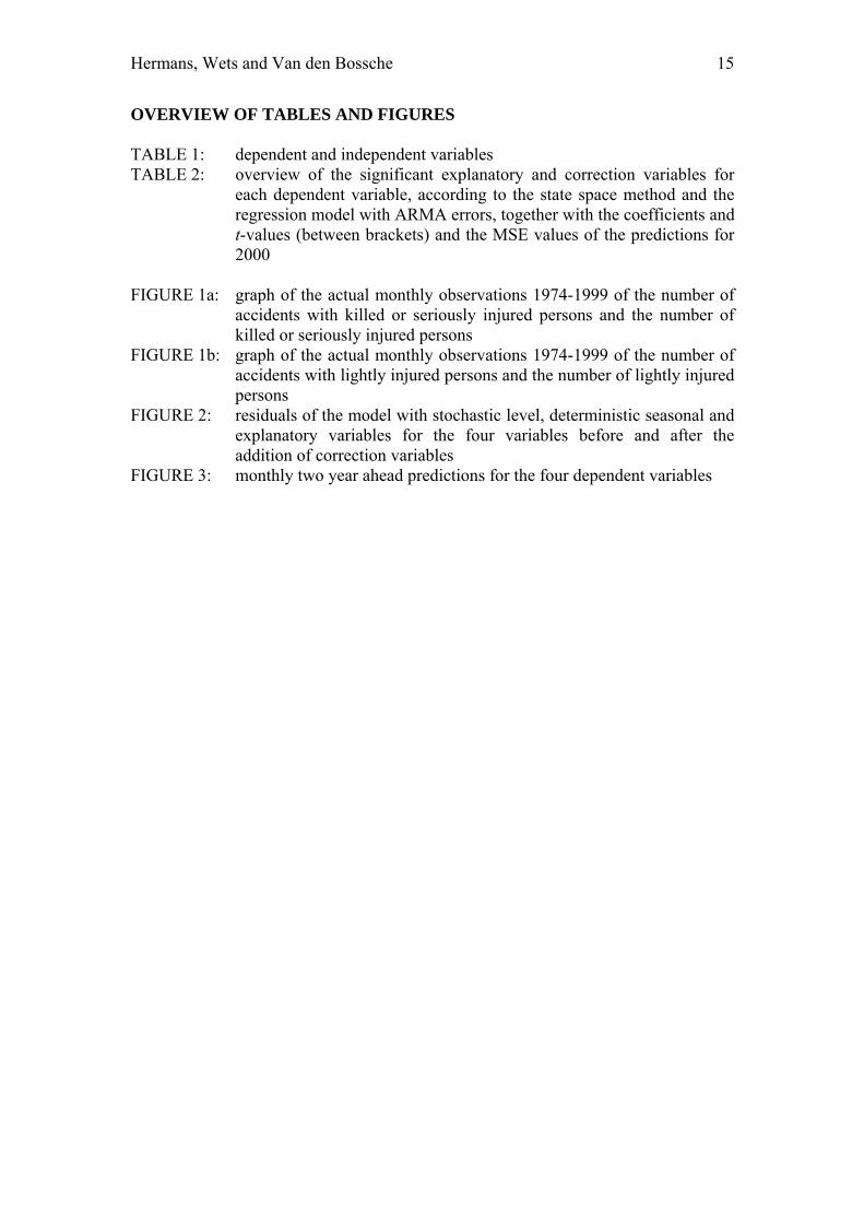
OVERVIEW OF TABLES AND FIGURES TABLE 1: dependent and independent variables TABLE 2: overview of the significant explanatory and correction variables for

each dependent variable, according to the state space method and the regression model with ARMA errors, together with the coefficients and t-values (between brackets) and the MSE values of the predictions for 2000

FIGURE 1a: graph of the actual monthly observations 1974-1999 of the number of

accidents with killed or seriously injured persons and the number of killed or seriously injured persons

FIGURE 1b: graph of the actual monthly observations 1974-1999 of the number of accidents with lightly injured persons and the number of lightly injured persons

FIGURE 2: residuals of the model with stochastic level, deterministic seasonal and explanatory variables for the four variables before and after the addition of correction variables

FIGURE 3: monthly two year ahead predictions for the four dependent variables


TABLE 1: dependent and independent variables Category Dependent variable Name

The (log-transformed) number of accidents with persons killed or seriously injured

LNACCKSI Number of accidents

The (log-transformed) number of accidents with lightly injured persons

LNACCLI

The (log-transformed) number of persons killed or seriously injured

LNPERKSI Number of casualties

The (log-transformed) number of persons lightly injured LNPERLI Category Independent variable Name

Law of June 1975 → mandatory seat belt use in the front seats

LAW0675

Law of November 1988 → introduction of zones with a speed limit of 30 km/h

LAW1188

Law of January 1992 → a.o. speed limit of 50 km/h in urban areas and 90 km/h at road sections with at least 2 by 2 lanes without separation

LAW0192

Law of December 1994 → 0.5‰ blood alcohol concentration imposed and higher fines in case of 0.8‰ or higher

LAW1294

Laws and regulations

Law of April 1996 → a vehicle driver should give right of way to pedestrians who are (or have the intention to) crossing the street

LAW0496

The quantity of precipitation (in mm) QUAPREC The monthly percentage of days with precipitation PDAYPREC The number of sunlight hours HRSSUN The monthly percentage of days with sunlight PDAYSUN The monthly percentage of days with frost PDAYFROST The monthly percentage of days with snow PDAYSNOW

Weather conditions

The monthly percentage of days with thunderstorm PDAYTHUN The percentage inflation INFLAT The (log-transformed) number of unemployed persons LNUNEMP The (log-transformed) number of car registrations LNCAR

Economic variables

The percentage of second-hand car registrations POLDNCAR


TABLE 2: overview of the significant explanatory and correction variables for each dependent variable, according to the state space method and the regression model with ARMA errors, together with the coefficients and t-values (between brackets) and the MSE values of the predictions for 2000

LNACCKSI LNACCLI LNPERKSI LNPERLI State Space Regression State Space Regression State Space Regression State Space Regression

Laws and regulations LAW0675 -0.132 (-3.31) -0.135 (-3.82) -0.062 (-2.13) -0.070 (-2.40) -0.180 (-4.07) -0.159 (-4.24) -0.109 (-3.35) -0.120 (-3.75) LAW0192 -0.062 (-1.87) -0.063 (-2.17) -0.071 (-2.50) -0.087 (-2.09) -0.076 (-2.11) -0.064 (-2.03) LAW1294 -0.109 (-2.72) -0.105 (-3.12) -0.104 (-2.50) -0.093 (-2.57) Weather conditions QUAPREC 0.001 (4.12) 0.001 (4.71) 0.001 (3.85) 0.001 (4.39) PDAYPREC 0.001 (3.34) 0.001 (2.60) 0.001 (2.84) 0.001 (4.04) 0.001 (4.02) 0.001 (2.69) 0.001 (2.88) HRSSUN 0.000 (3.92) 0.001 (5.35) 0.001 (4.99) 0.001 (5.38) 0.001 (4.48) 0.001 (4.80) 0.000 (3.82) 0.000 (4.17) PDAYFROST -0.002 (-5.93) -0.001 (-5.77) -0.001 (-5.73) -0.001 (-5.63) -0.001 (-4.82) -0.001 (-4.81) -0.001 (-4.44) -0.001 (-4.36) PDAYTHUN 0.001 (2.12) 0.001 (2.06) 0.001 (2.03) 0.001 (1.93) Economic variables LNUNEMP 0.117 (1.69) LNCAR -0.078 (-2.11) Correction variables JAN79 -0.553 (-10.02) -0.574 (-12.05) -0.456(-10.02) -0.441 (-10.40) -0.558 (-9.72) -0.550 (-10.75) -0.464 (-9.51) -0.458 (-9.97) JAN84 -0.450 (-9.28) -0.449 (-9.87) JAN85 -0.277 (-5.04) -0.282 (-5.85) -0.2711 (-6.00) -0.2852 (-6.80) -0.297(-5.22) -0.289 (-5.62) -0.276 (-5.67) -0.294 (-6.46) FEB97 -0.118 (-2.15) -0.128 (-2.66) -0.2033 (-4.50) -0.2181 (-5.08) -0.130 (-2.28) -0.124 (-2.31) -0.214 (-4.41) -0.238 (-5.09) Forecasting measure MSE(12) 0.0050 0.0046 0.0034 0.0052 0.0070 0.0063 0.0036 0.0052


1975 1980 1985 1990 1995 2000

750

1000

1250

1500

1750

2000

2250 NACCKSI NPERKSI

_____________________________________________________________________ FIGURE 1a: graph of the actual monthly observations 1974-1999 of the number of accidents with killed or seriously injured persons (lower) and the number of killed or seriously injured persons (upper)

1975 1980 1985 1990 1995 2000

2000

2500

3000

3500

4000

4500

5000

5500

6000

6500

NACCLI NPERLI

_____________________________________________________________________ FIGURE 1b: graph of the actual monthly observations 1974-1999 of the number of accidents with lightly injured persons (lower) and the number of lightly injured persons (upper)


1975 1980 1985 1990 1995 2000

-5

0

5 Residual LNACCKSI

1975 1980 1985 1990 1995 2000

-2.5

0.0

2.5 Residual LNACCKSI

1975 1980 1985 1990 1995 2000

-5

0

5 Residual LNACCLI

1975 1980 1985 1990 1995 2000

-202 Residual LNACCLI

1975 1980 1985 1990 1995 2000

-5

0

Residual LNPERKSI

1975 1980 1985 1990 1995 2000

-2.5

0.0

2.5 Residual LNPERKSI

1975 1980 1985 1990 1995 2000

-5

0

5 Residual LNPERLI

1975 1980 1985 1990 1995 2000

-2.5

0.0

2.5 Residual LNPERLI

_____________________________________________________________________ FIGURE 2: residuals of the model with stochastic level, deterministic seasonal and explanatory variables for the four variables before (left) and after (right) the addition of correction variables


2000 2001 2002

6.4

6.6

6.8

LNACCKSI Forecast

2000 2001 2002

7.8

8.0

8.2

LNACCLI Forecast

2000 2001 2002

6.50

6.75

7.00

LNPERKSI Forecast

2000 2001 2002

8.2

8.4

8.6

LNPERLI Forecast

_____________________________________________________________________ FIGURE 3: monthly two year ahead predictions for the four dependent variables The darkest lines represent the actual observations. Predictions together with the upper and lower bounds of the prediction interval are in lighter grey.


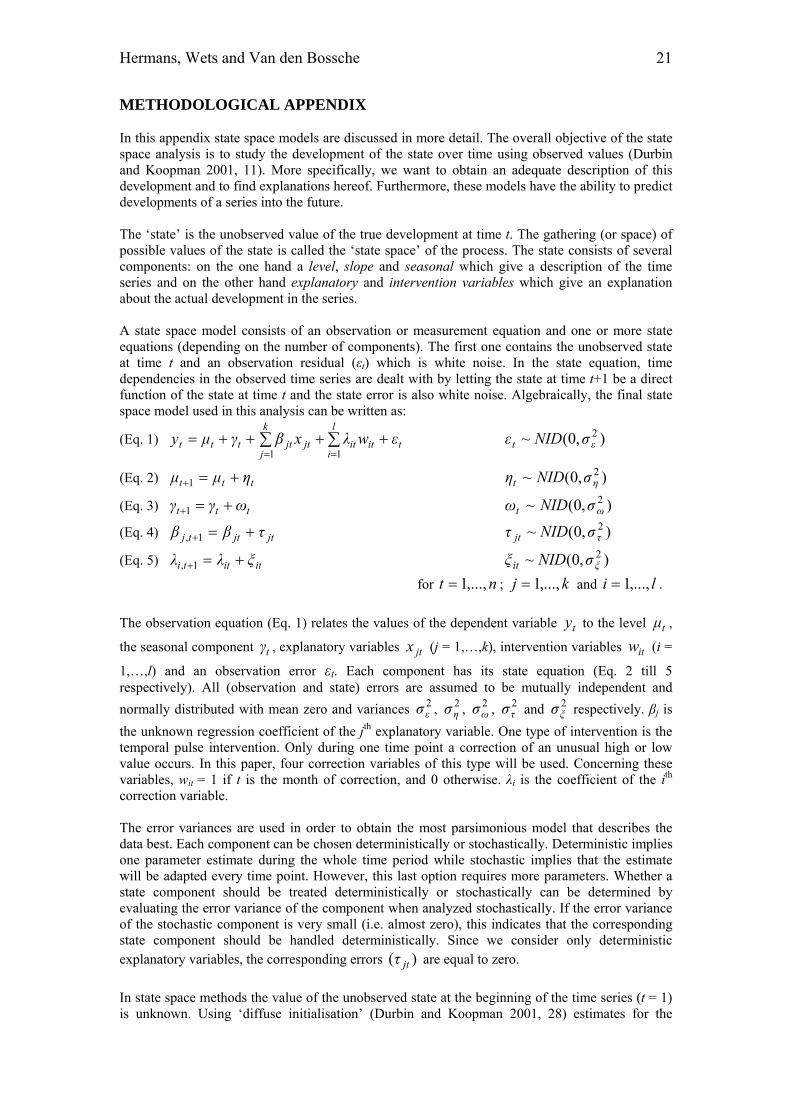
METHODOLOGICAL APPENDIX In this appendix state space models are discussed in more detail. The overall objective of the state space analysis is to study the development of the state over time using observed values (Durbin and Koopman 2001, 11). More specifically, we want to obtain an adequate description of this development and to find explanations hereof. Furthermore, these models have the ability to predict developments of a series into the future. The ‘state’ is the unobserved value of the true development at time t. The gathering (or space) of possible values of the state is called the ‘state space’ of the process. The state consists of several components: on the one hand a level, slope and seasonal which give a description of the time series and on the other hand explanatory and intervention variables which give an explanation about the actual development in the series. A state space model consists of an observation or measurement equation and one or more state equations (depending on the number of components). The first one contains the unobserved state at time t and an observation residual (εt) which is white noise. In the state equation, time dependencies in the observed time series are dealt with by letting the state at time t+1 be a direct function of the state at time t and the state error is also white noise. Algebraically, the final state space model used in this analysis can be written as:

(Eq. 1) t

l

iitit

k

jjtjtttt εwλxβγµy ++++= ∑∑

== 11 ),0(~ 2

εt σNIDε

(Eq. 2) ttt ηµµ +=+1 ),0(~ 2ηt σNIDη

(Eq. 3) ttt ωγγ +=+1 ),0(~ 2ωt σNIDω

(Eq. 4) jtjttj τββ +=+1, ),0(~ 2τjt σNIDτ

(Eq. 5) ititti ξλλ +=+1, ),0(~ 2ξit σNIDξ

for nt ,...,1= ; kj ,...,1= and li ,...,1= .

The observation equation (Eq. 1) relates the values of the dependent variable ty to the level tµ ,

the seasonal component tγ , explanatory variables jtx (j = 1,…,k), intervention variables itw (i =

1,…,l) and an observation error εt. Each component has its state equation (Eq. 2 till 5 respectively). All (observation and state) errors are assumed to be mutually independent and normally distributed with mean zero and variances 2

εσ , 2ησ , 2

ωσ , 2τσ and 2

ξσ respectively. βj is the unknown regression coefficient of the jth explanatory variable. One type of intervention is the temporal pulse intervention. Only during one time point a correction of an unusual high or low value occurs. In this paper, four correction variables of this type will be used. Concerning these variables, wit = 1 if t is the month of correction, and 0 otherwise. λi is the coefficient of the ith correction variable. The error variances are used in order to obtain the most parsimonious model that describes the data best. Each component can be chosen deterministically or stochastically. Deterministic implies one parameter estimate during the whole time period while stochastic implies that the estimate will be adapted every time point. However, this last option requires more parameters. Whether a state component should be treated deterministically or stochastically can be determined by evaluating the error variance of the component when analyzed stochastically. If the error variance of the stochastic component is very small (i.e. almost zero), this indicates that the corresponding state component should be handled deterministically. Since we consider only deterministic explanatory variables, the corresponding errors )( jtτ are equal to zero. In state space methods the value of the unobserved state at the beginning of the time series (t = 1) is unknown. Using ‘diffuse initialisation’ (Durbin and Koopman 2001, 28) estimates for the


unknown parameters are obtained. Also none of the observation and state error variances are known. The estimation of all these parameters can be obtained with an iterative process, using the maximum likelihood principle.

Documents

Frequency and Severity of Belgian Road Traffic Accidents Studied by State Space Methods€¦ · · 2011-11-25The methodology used throughout the analysis is state space methods