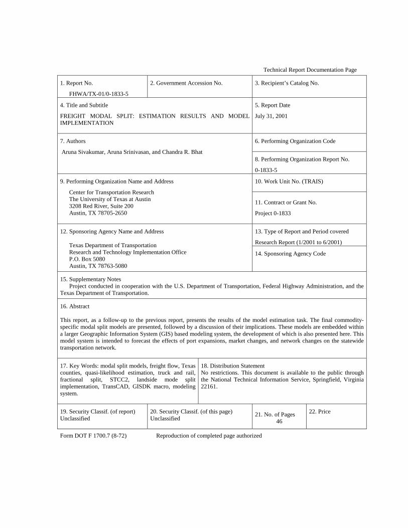
Technical Report Documentation Page

1. Report No.

FHWA/TX-01/0-1833-5

2. Government Accession No. 3. Recipient’s Catalog No.

4. Title and Subtitle

FREIGHT MODAL SPLIT: ESTIMATION RESULTS AND MODEL IMPLEMENTATION

5. Report Date

July 31, 2001

6. Performing Organization Code

7. Authors

Aruna Sivakumar, Aruna Srinivasan, and Chandra R. Bhat 8. Performing Organization Report No.

0-1833-5

10. Work Unit No. (TRAIS)

9. Performing Organization Name and Address

Center for Transportation Research The University of Texas at Austin 3208 Red River, Suite 200 Austin, TX 78705-2650

11. Contract or Grant No.

Project 0-1833

13. Type of Report and Period covered

Research Report (1/2001 to 6/2001)

12. Sponsoring Agency Name and Address

Texas Department of Transportation Research and Technology Implementation OfficeP.O. Box 5080 Austin, TX 78763-5080

14. Sponsoring Agency Code

15. Supplementary Notes Project conducted in cooperation with the U.S. Department of Transportation, Federal Highway Administration, and the

Texas Department of Transportation.

16. Abstract This report, as a follow-up to the previous report, presents the results of the model estimation task. The final commodity-specific modal split models are presented, followed by a discussion of their implications. These models are embedded within a larger Geographic Information System (GIS) based modeling system, the development of which is also presented here. This model system is intended to forecast the effects of port expansions, market changes, and network changes on the statewide transportation network.

17. Key Words: modal split models, freight flow, Texas counties, quasi-likelihood estimation, truck and rail, fractional split, STCC2, landside mode split implementation, TransCAD, GISDK macro, modeling system.

18. Distribution Statement No restrictions. This document is available to the public through the National Technical Information Service, Springfield, Virginia 22161.

19. Security Classif. (of report) Unclassified

20. Security Classif. (of this page) Unclassified

21. No. of Pages

46

22. Price

Form DOT F 1700.7 (8-72) Reproduction of completed page authorized

�

FREIGHT MODAL SPLIT:

ESTIMATION RESULTS AND MODEL IMPLEMENTATION

by

Aruna Sivakumar, Aruna Srinivasan, and Chandra R. Bhat

Research Report Number 0-1833-5

Research Project 0-1833 Infrastructure Impacts and Operational Requirements Associated with

the Next-Generation Container Ships (Megaships) on the Texas Transportation System

Conducted for the

TEXAS DEPARTMENT OF TRANSPORTATION

in cooperation with the

U.S. DEPARTMENT OF TRANSPORTATION

FEDERAL HIGHWAY ADMINISTRATION

by the

CENTER FOR TRANSPORTATION RESEARCH

Bureau of Engineering Research

THE UNIVERSITY OF TEXAS AT AUSTIN

July 2001

iv

v

DISCLAIMERS

The contents of this report reflect the views of the authors, who are responsible for the facts and the accuracy of the data presented herein. The contents do not necessarily reflect the official views or policies of either the Federal Highway Administration (FHWA) or the Texas Department of Transportation (TxDOT). This report does not constitute a standard, specification, or regulation.

There was no invention or discovery conceived or first actually reduced to

practice in the course of or under this contract, including any art, method, process, machine, manufacture, design or composition of matter, or any new and useful improvement thereof, or any variety of plant, which is or may be patentable under the patent laws of the United States of America or any foreign country.

NOT INTENDED FOR CONSTRUCTION, BIDDING, OR PERMIT PURPOSES

Chandra R. Bhat

Research Supervisor

ACKNOWLEDGMENTS

The research supervisor wishes to recognize the support and participation of Robert Harrison, senior research scientist (CTR); Michael Bomba, LBJ School graduate student intern; and the crucial help and direction provided by the TransCAD support staff. Also significant to the accomplishment of this project has been the involvement and direction of the Texas Department of Transportation (TxDOT) project steering committee, which includes the Project Director Raul Cantu (TPP) and project monitoring committee members Jim Randall (MMO), Kelly Kirkland (MMO), Chris Olavson (HOU), and Carol Nixon (HOU).

Chandra R. Bhat, Research Supervisor

Research performed in cooperation with the Texas Department of Transportation and

the U.S. Department of Transportation, Federal Highway Administration.

vi

vii

TABLE OF CONTENTS

SECTION 1. INTRODUCTION ............................................................................................................1 SECTION 2. MODE SPLIT ESTIMATION RESULTS AND DISCUSSION .....................................3 2.1. Impedance......................................................................................................................4 2.2. Zonal Socioeconomics...................................................................................................5 2.3. Other Variables ..............................................................................................................6 SECTION 3. IMPLEMENTATION WITHIN A GEOGRAPHIC INFORMATION SYSTEM PLATFORM...........................................................................................................................................7 3.1. Implementation Framework...........................................................................................7 3.2. Sequence of Operations in Application .........................................................................8 SECTION 4. USERS’ GUIDE TO THE GEOGRAPHIC INFORMATION SYSTEM MODELING SYSTEM ........................................................................................................................13 SECTION 5. CONCLUSION...............................................................................................................17 APPENDIX A. GISDK CODE.............................................................................................................19 APPENDIX B. SAMPLE INPUT DATA TABLES ............................................................................37

LIST OF TABLES

TABLE 1. ESTIMATION RESULTS: BEST SPECIFICATION MODEL BY COMMODITY TYPE ......................................................................................................................................................5 TABLE 2. INPUT DATA TABLES.....................................................................................................13 TABLE 3. THROUGHPUTS AND MARKETS SERVED.................................................................37 TABLE 4. ZONAL SOCIOECONOMICS ..........................................................................................37 TABLE 5. IMPEDANCE DATA TABLE ...........................................................................................37 TABLE 6. MODAL SPLIT MODEL PARAMETERS........................................................................38

viii

LIST OF FIGURES

FIGURE 1. FLOWCHART: SEQUENCE OF OPERATIONS ...........................................................10

1

1. INTRODUCTION

An evaluation of the potential landside traffic impacts of international economic

expansion in maritime container freight trade is necessary to plan an efficient and

productive transportation system. The focus of this project is to contribute toward such an

evaluation of the potential landside traffic impacts by developing a modeling system that

can forecast the effects of port expansions, market changes, and network changes on the

statewide transportation network. The modeling system consists of two main components

– the modal split model and the network assignment model. Previously, in Report 0-

1833-4, we discussed the conceptual framework for the modal split model, the structure

for the model, and the data sources and data assembly procedures for model estimation.

In this report, we present the estimation results for the modal split model, discuss the

network assignment model, and describe the procedures used to integrate the modal split

and network assignment within a Geographic Information System (GIS) platform. The

resulting GIS-based modeling system is a flexible tool that can be used to study the

impacts of economic expansions and policy implementations on statewide road and rail

traffic.

The remainder of this report is organized as follows. Section 2 presents and interprets

the model estimation results. Section 3 discusses the procedures adopted to embed the

modal split model within a GIS interface and integrate the modal split model with

network assignment. Section 4 provides step-by-step instructions for the execution of the

GIS-based application. Section 5 concludes the report.

2

3

2. MODE SPLIT ESTIMATION RESULTS AND DISCUSSION

Report 0-1833-4 discusses the steps undertaken to assemble the data sets for mode

split. The primary data source in data assembly is the Reebie data. At the end of the data

assembly process, seven commodity-specific data sets were assembled for each of seven

aggregate commodity types. The aggregate commodity types are (a) agriculture and

related products, (b) hazardous materials, (c) construction materials, (d) food and related

products, (e) manufacturing products, (f) machinery and equipment, and (g) mixed freight

shipments. The dependent variable of analysis in each of the seven data sets is the

fraction of total tonnage moved by rail between each pair of counties within Texas. The

objective in the estimation stage is to determine the impact of relevant exogenous

variables (such as travel impedance, distance of haul, shipment size, and county

socioeconomic characteristics) on the fraction of tonnage moved by rail (as opposed to

the fraction moved by road). A binary fractional split model is used for this purpose

(details of the fractional split model formulation have been provided in Section 3 of the

previous report and will not be repeated here).

In this report, we present the estimation results for five of the seven commodity types

identified earlier. This is because two of the commodity groups (machinery and

equipment, and mixed freight shipments) have a rail share of zero for 99.9% of the

county-to-county commodity flows. The dominance of the road transport mode for these

two commodities leads to inadequate variation in the rail fraction, which in turn makes it

impossible to estimate a mode split model for these commodities.

4

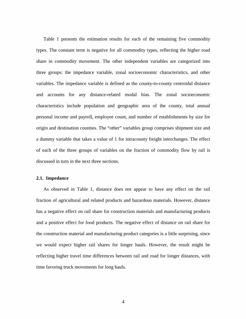
Table 1 presents the estimation results for each of the remaining five commodity

types. The constant term is negative for all commodity types, reflecting the higher road

share in commodity movement. The other independent variables are categorized into

three groups: the impedance variable, zonal socioeconomic characteristics, and other

variables. The impedance variable is defined as the county-to-county centroidal distance

and accounts for any distance-related modal bias. The zonal socioeconomic

characteristics include population and geographic area of the county, total annual

personal income and payroll, employee count, and number of establishments by size for

origin and destination counties. The “other” variables group comprises shipment size and

a dummy variable that takes a value of 1 for intracounty freight interchanges. The effect

of each of the three groups of variables on the fraction of commodity flow by rail is

discussed in turn in the next three sections.

2.1. Impedance

As observed in Table 1, distance does not appear to have any effect on the rail

fraction of agricultural and related products and hazardous materials. However, distance

has a negative effect on rail share for construction materials and manufacturing products

and a positive effect for food products. The negative effect of distance on rail share for

the construction material and manufacturing product categories is a little surprising, since

we would expect higher rail shares for longer hauls. However, the result might be

reflecting higher travel time differences between rail and road for longer distances, with

time favoring truck movements for long hauls.

5

Table 1. Estimation results: best specification model by commodity type

2.2. Zonal Socioeconomics

The effect of zonal socioeconomics indicates that rail is the preferred mode when the

origin and destination zones have a large number of establishments. This might be a

result of better rail network infrastructure around zones with a large number of

Variables

Agricultural & Related

Products

Hazardous Materials

Construction Materials

Food & Related Products

Manufacturing Products

Parameter t-stat Parameter t-stat Parameter t-stat Parameter t-stat Parameter t-stat

Constant -3.4033 -6.70 -5.2345 -24.69 -4.5855 -27.58 -6.6887 -10.24 -6.1582 -22.80

Impedance distance - - - - -0.2059 -3.69 0.2947 2.89 -0.1616 -2.16

Origin socioeconomics Origin population -77.9598 -5.06 4.4291 2.16 -7.3743 -2.46 -4.5946 -1.70 5.7014 1.89 Origin area - - 0.2851 1.98 0.5463 7.02 -0.7420 -1.23 0.5048 3.34 Origin personal income 2.3087 3.67 -0.1135 -1.38 0.1735 1.37 0.3432 2.40 -0.1520 -1.55 Origin payroll -0.8890 -4.48 0.0471 1.10 -0.2714 -3.36 -0.1833 -2.92 - - Origin employee count -106.1313 -2.48 -15.6901 -5.05 - - - - - - Origin # estab (1-500) 14.9046 4.14 1.1626 2.77 1.2108 2.93 - - -0.7482 -1.06 Origin # estab (500-1k) 25.7713 1.59 - - - - 3.5599 2.31 6.0321 2.52 Origin # estab (> 1000) 21.4750 4.35 3.9868 4.32 2.2923 2.47 - - -3.2057 -3.42

Dest socioeconomics Dest population - - 8.0581 4.49 - - -5.8814 -1.56 5.2057 2.50 Dest area -0.4809 -1.13 0.2103 2.13 - - 0.5251 3.98 0.4174 3.75 Dest personal income 0.1870 2.11 -0.1634 -1.79 -0.1411 -2.44 - - -0.1715 -1.69 Dest payroll - - 0.0946 1.98 - - -0.1536 -2.30 -0.0539 -1.04 Dest employee count - - -9.3254 -3.21 -16.0850 -3.82 -17.8542 -1.74 -4.8414 -1.24 Dest # estab (1-500) - - - - 1.2074 4.57 1.8093 2.00 - - Dest # estab (500-1000) - - - - 8.3067 3.40 12.1688 2.20 4.2836 1.53 Dest # estab (> 1000) -1.9983 -3.11 2.0354 2.17 - - - - - -

Other variables Shipment size (tons) 0.8261 10.30 0.0002 1.89 0.0031 6.10 - - - - intracounty dummy - - 0.7453 1.32 - - - - - -

Log-Likelihood -105.4595 -1024.130 -1039.385 -284.3056 -605.1219 Restricted Log-Likelihood -577.317 -1763.628 -1811.437 -533.2275 -1089.553

chi-sqd. 943.7151 1478.9970 1544.1030 497.8439 968.8631

6

establishments. On the other hand, truck is the preferred mode when the origin and

destination zones have a large number of employees. The effect of the other zonal

socioeconomic characteristics may be similarly interpreted.

2.3. Other Variables

The estimation results indicate that rail is the preferred mode for shipments of larger

size and this is intuitive. However, this result applies only for agricultural products,

hazardous materials, and construction materials. The intracounty dummy variable is

significant only for hazardous materials. The sign on the parameter indicates that rail is

the preferred mode for shipping hazardous materials within a county.

7

3. IMPLEMENTATION WITHIN A GEOGRAPHIC INFORMATION SYSTEM

PLATFORM

3.1. Implementation Framework

The application of the mode split models discussed in the previous section is

straightforward. The inputs required for application include throughput at the port by

commodity type, markets served by the port and their socioeconomic characteristics, and

the impedance measure between the port and each market. These inputs can correspond

to the current situation or a projected future situation. The predicted mode splits can then

be translated into rail and truck freight movements on the statewide transportation

networks using a network assignment procedure.

The spatial nature of the application problem in the current context makes

implementation within a Geographic Information System framework appealing. A GIS-

based model implementation package provides the user with a realistic and easily

comprehensible visualization of commodity flows on the Texas transportation networks.

In our project, we use TransCAD as the application platform. TransCAD is a flexible GIS

platform developed by Caliper Corporation, Inc. It has an embedded network assignment

procedure, which is particularly helpful in obtaining link flows on the road and rail

networks from the predicted county-to-county road and rail mode splits. Specifically, we

use the all-or-nothing assignment procedure of TransCAD to load commodity flows onto

the road and rail networks. The detailed sequence of operations during application is

discussed in the next section. (The development of the user interface in TransCAD is

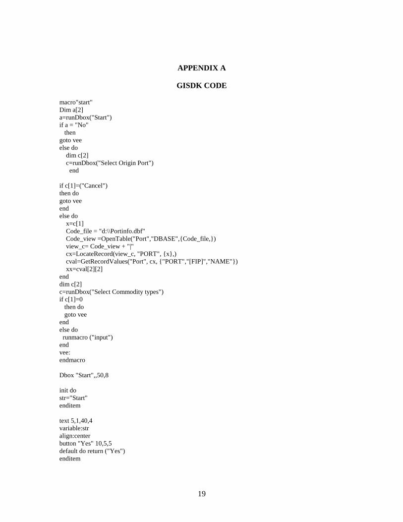
8

carried out by coding in the Caliper script (GISDK); the actual code for the entire

application package is provided in Appendix A.)

3.2. Sequence of Operations in Application

The sequence of operations during the application of the GIS-based modeling

package is presented in Figure 1. The figure describes the structure of the GIS-based

platform from a user’s perspective.

The procedure starts with the options of either performing a quick demonstration or

going directly to the application. The demonstration provides the user with a sample

application (see instructions in Section 4). The demonstration will be particularly useful

for first-time users, since the application requires specific input data formats. Users

familiar with the procedure can skip the demonstration and proceed directly to the

implementation.

The first stage of the application process involves specification of the inputs. The

program requires the following inputs: (a) the port of origin, chosen from a given list of

Gulf ports, (b) the commodity types passing through the port, chosen from a given list of

seven aggregate commodity types, (c) data table of markets served and commodity-

specific throughputs to each of the destination markets, (d) data table with the

socioeconomic characteristics of origin and destination counties, and impedance data for

all origin-destination county pairs, and (e) the sensitivity of rail share to each of the input

variables, which is essentially the model parameters estimated. Of these inputs, default

socioeconomic characteristics, impedances, and modal split model parameters are

embedded within the modeling system. However, the modeling system is capable of

9

accepting user-defined data for each of these. This provision makes the system spatially

and temporally transferable.

The modal split model uses the input data to estimate rail and road mode shares. The

results are displayed on a digitized map of Texas. The commodity-specific road and rail

tonnages transported to each of the destination markets form an attribute of the

destination zones, and can be viewed by clicking the market of interest. This data is also

available in a database format, which forms the input to the network assignment

procedure and can be exported to other applications. Following the computation of modal

splits for each port to destination county interchange, network assignment is performed

and the road and rail tonnages are loaded onto the shortest path between the origin port

and each of the destination markets. The freight tonnage forms an attribute of the links of

the road and rail networks and clicking on any specific link displays the total tonnage

moved over that link.

10

Fig. 1. Flowchart: sequence of operations

Welcome

���Select – Demo Start at once

Choose Port of origin

Select Commodity types

System Prompts: Input throughput data

System prompts: default or user input socioeconomics and impedance

Picks up relevant embedded data on demographics and distances

Prompts user to input data on demographics and distance matrix

User Input data

Picks up relevant data on demographics and distances

Default data

System prompts: default modal split model or user-input model

Input (a) in text

Input (b) in text

Input (c) in text

Input (d) in text

Input (e) in text

11

Fig. 1. Flowchart: sequence of operations, continued

Default model User input model

System prompts user to input model coefficient table

Picks up data from user input coefficient table

Picks up data from embedded coefficient table

Displays the origin and destination counties

Displays the rail and road shares by commodity types for the counties on user click

Message display: Mode Split stage completed

Displays the route taken from the origin to the markets served by commodity types

Message display: Traffic Assignment stage completed

End

12

13

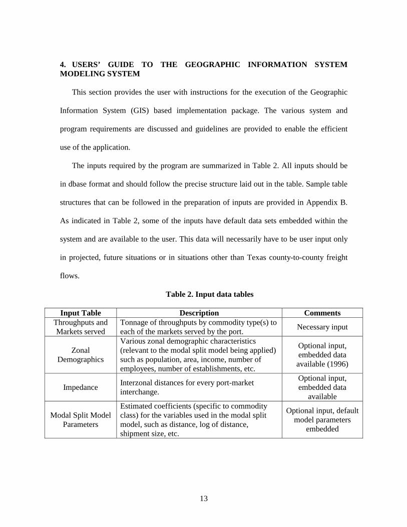
4. USERS’ GUIDE TO THE GEOGRAPHIC INFORMATION SYSTEM MODELING SYSTEM

This section provides the user with instructions for the execution of the Geographic

Information System (GIS) based implementation package. The various system and

program requirements are discussed and guidelines are provided to enable the efficient

use of the application.

The inputs required by the program are summarized in Table 2. All inputs should be

in dbase format and should follow the precise structure laid out in the table. Sample table

structures that can be followed in the preparation of inputs are provided in Appendix B.

As indicated in Table 2, some of the inputs have default data sets embedded within the

system and are available to the user. This data will necessarily have to be user input only

in projected, future situations or in situations other than Texas county-to-county freight

flows.

Table 2. Input data tables

Input Table Description Comments Throughputs and Markets served

Tonnage of throughputs by commodity type(s) to each of the markets served by the port.

Necessary input

Zonal Demographics

Various zonal demographic characteristics (relevant to the modal split model being applied) such as population, area, income, number of employees, number of establishments, etc.

Optional input, embedded data available (1996)

Impedance Interzonal distances for every port-market interchange.

Optional input, embedded data

available

Modal Split Model Parameters

Estimated coefficients (specific to commodity class) for the variables used in the modal split model, such as distance, log of distance, shipment size, etc.

Optional input, default model parameters

embedded

14

The outputs of the modal split and traffic assignment steps are available in both a

tabular form as well as in the form of a digitized display overlaid on the map of Texas. At

the end of the mode split procedure, the map of Texas is displayed with the origin and the

destination counties highlighted in black and blue, respectively. These zones are linked to

the corresponding mode split data, allowing for a quick visual survey of the mode split

with reference to the geography of the zones. Pure data tables that form the backdrop to

the visual display are also created. These tables provide the commodity-specific tonnages

transported by road and rail, which can be further used as inputs into the network

assignment procedure.

In the traffic assignment step, the rail and road tonnages are loaded onto the Texas

road and rail networks, following an all-or-nothing assignment procedure. The total

freight tonnage (across all commodities) is stored as an attribute of the link that forms

part of the route between each origin-destination pair. The output is displayed as route

systems on the Texas road and rail networks. Selecting a link opens the attribute table

corresponding to that link and displays the total tons of freight of all commodity types

transported on that link. This data is also available in dbase format and can be exported to

other applications.

The following step-by-step instructions will serve as a user guideline to run a sample

application in the modeling system. This sample run uses the default data sets and a

sample input data file provided in the system.

a) Open TransCAD and choose Tools – Add Ins. Select the modeling system “TX Ports

– freight flows”.

15

b) From the welcome screen, which provides the user with two options demo or start

at once — select the “Demo” option.

c) Select the origin port from the drop-down menu as “Texas City”. Click on OK.

d) Select all the commodity types from the drop-down menu that follows.

e) The next dialog box requires the “throughputs and markets served” input data table. A

sample input table is stored within the system for demonstration purposes. From the

dialog box that opens, select the input data file “Inputs.dbf”.

f) Click on YES when the system prompts you to use the default data set for zonal

sociodemographics.

g) The program displays all the variables used in the default model and the data for the

model is provided in the input table. Click on OK to continue.

h) Click on YES when the system prompts the user to use the default model.

i) The input stage is now complete. The system performs the modal split and the output

appears on the screen as a display of the map of Texas, with the origin port shaded in

black and the destination markets in blue. Click on the info tool, the “i” icon in the

TransCAD toolbox, and click on any of the markets to view a table with the

commodity-specific tonnages transported by road and rail from the port of Texas

City. The output data for the mode split step is available in a separate database file.

j) Click on OK when the system displays the message that the mode split stage has been

completed. This prompts the system to proceed with the network assignment step.

k) The output of the network assignment procedure is viewed on a map of Texas with

the statewide road and rail networks. The routes along which the commodities are

16

transported between the origin and the destination counties are displayed as a route

system. Click on the info tool, the “i” icon in the TransCAD toolbox, and click on any

link on the network to obtain the total freight flow on the link. The link tonnages are

available in road- and rail-specific database files.

l) When the system displays a message that the traffic assignment stage is completed,

click on OK to exit the program.

17

5. CONCLUSION

This report presents the results for commodity-specific modal split models estimated

using Reebie data. A Geographic Information System (GIS) based modeling system

developed within TransCAD to implement the modal split models and to integrate the

output of these models with a network assignment procedure is discussed. The resulting

TransCAD-based application platform provides a flexible tool to analyze the impacts of

port expansion and market changes on commodity flows on the Texas road and rail

networks.

18

19

APPENDIX A

GISDK CODE

macro"start" Dim a[2] a=runDbox("Start") if a = "No" then goto vee else do dim c[2] c=runDbox("Select Origin Port") end if c[1]=("Cancel") then do goto vee end else do x=c[1] Code_file = "d:\\Portinfo.dbf" Code_view =OpenTable("Port","DBASE",{Code_file,}) view_c= Code_view + "|" cx=LocateRecord(view_c, "PORT", {x},) cval=GetRecordValues("Port", cx, {"PORT","[FIP]","NAME"}) xx=cval[2][2] end dim c[2] c=runDbox("Select Commodity types") if c[1]=0 then do goto vee end else do runmacro ("input") end vee: endmacro Dbox "Start",,50,8 init do str="Start" enditem text 5,1,40,4 variable:str align:center button "Yes" 10,5,5 default do return ("Yes") enditem

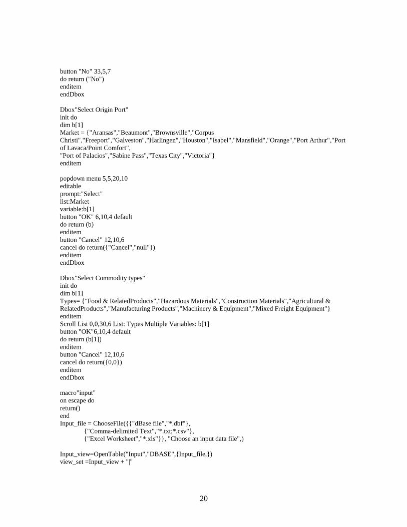
20

button "No" 33,5,7 do return ("No") enditem endDbox Dbox"Select Origin Port" init do dim b[1] Market = {"Aransas","Beaumont","Brownsville","Corpus Christi","Freeport","Galveston","Harlingen","Houston","Isabel","Mansfield","Orange","Port Arthur","Port of Lavaca/Point Comfort", "Port of Palacios","Sabine Pass","Texas City","Victoria"} enditem popdown menu 5,5,20,10 editable prompt:"Select" list:Market variable:b[1] button "OK" 6,10,4 default do return (b) enditem button "Cancel" 12,10,6 cancel do return({"Cancel","null"}) enditem endDbox Dbox"Select Commodity types" init do dim b[1] Types= {"Food & RelatedProducts","Hazardous Materials","Construction Materials","Agricultural & RelatedProducts","Manufacturing Products","Machinery & Equipment","Mixed Freight Equipment"} enditem Scroll List 0,0,30,6 List: Types Multiple Variables: b[1] button "OK"6,10,4 default do return (b[1]) enditem button "Cancel" 12,10,6 cancel do return({0,0}) enditem endDbox macro"input" on escape do return() end Input_file = ChooseFile({{"dBase file","*.dbf"}, {"Comma-delimited Text","*.txt;*.csv"}, {"Excel Worksheet","*.xls"}}, "Choose an input data file",) Input_view=OpenTable("Input","DBASE",{Input_file,}) view_set =Input_view + "|"

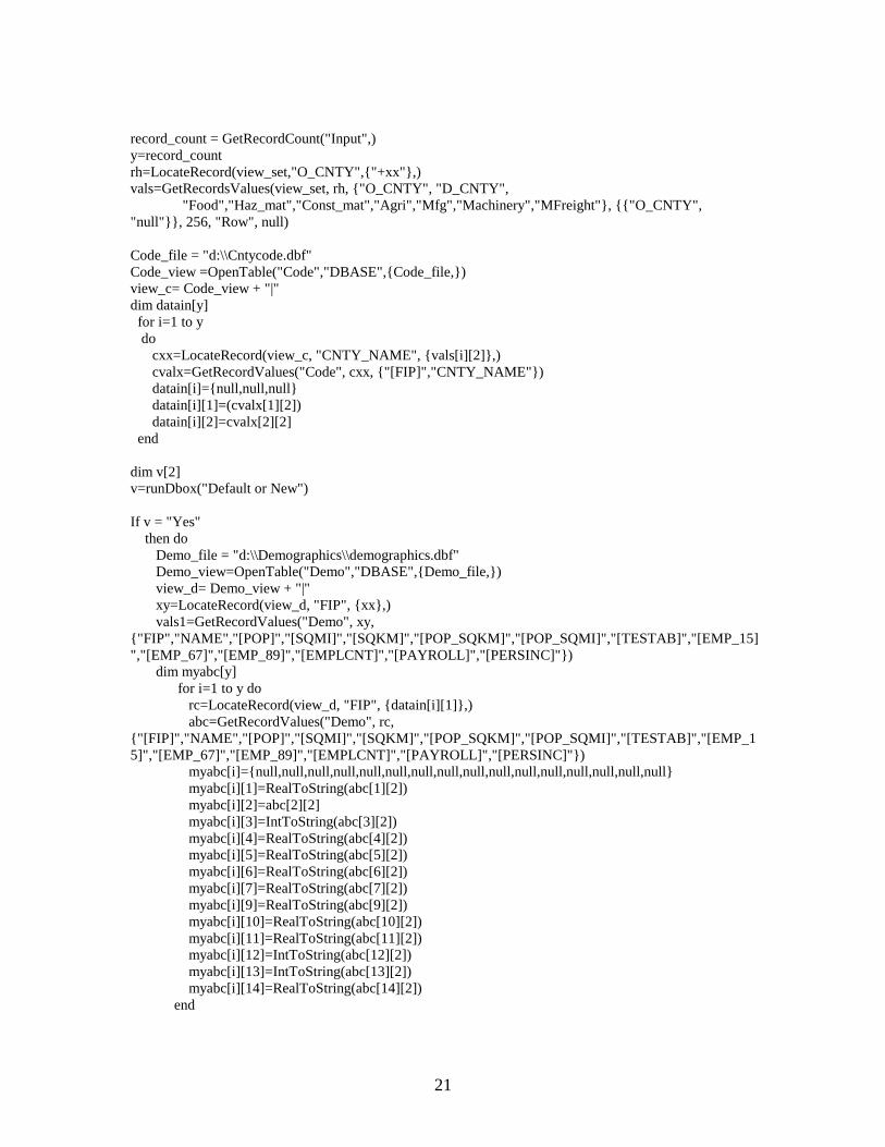
21

record_count = GetRecordCount("Input",) y=record_count rh=LocateRecord(view_set,"O_CNTY",{"+xx"},) vals=GetRecordsValues(view_set, rh, {"O_CNTY", "D_CNTY", "Food","Haz_mat","Const_mat","Agri","Mfg","Machinery","MFreight"}, {{"O_CNTY", "null"}}, 256, "Row", null) Code_file = "d:\\Cntycode.dbf" Code_view =OpenTable("Code","DBASE",{Code_file,}) view_c= Code_view + "|" dim datain[y] for i=1 to y do cxx=LocateRecord(view_c, "CNTY_NAME", {vals[i][2]},) cvalx=GetRecordValues("Code", cxx, {"[FIP]","CNTY_NAME"}) datain[i]={null,null,null} datain[i][1]=(cvalx[1][2]) datain[i][2]=cvalx[2][2] end dim v[2] v=runDbox("Default or New") If v = "Yes" then do Demo_file = "d:\\Demographics\\demographics.dbf" Demo_view=OpenTable("Demo","DBASE",{Demo_file,}) view_d= Demo_view + "|" xy=LocateRecord(view_d, "FIP", {xx},) vals1=GetRecordValues("Demo", xy, {"FIP","NAME","[POP]","[SQMI]","[SQKM]","[POP_SQKM]","[POP_SQMI]","[TESTAB]","[EMP_15]","[EMP_67]","[EMP_89]","[EMPLCNT]","[PAYROLL]","[PERSINC]"}) dim myabc[y] for i=1 to y do rc=LocateRecord(view_d, "FIP", {datain[i][1]},) abc=GetRecordValues("Demo", rc, {"[FIP]","NAME","[POP]","[SQMI]","[SQKM]","[POP_SQKM]","[POP_SQMI]","[TESTAB]","[EMP_15]","[EMP_67]","[EMP_89]","[EMPLCNT]","[PAYROLL]","[PERSINC]"}) myabc[i]={null,null,null,null,null,null,null,null,null,null,null,null,null,null,null,null} myabc[i][1]=RealToString(abc[1][2]) myabc[i][2]=abc[2][2] myabc[i][3]=IntToString(abc[3][2]) myabc[i][4]=RealToString(abc[4][2]) myabc[i][5]=RealToString(abc[5][2]) myabc[i][6]=RealToString(abc[6][2]) myabc[i][7]=RealToString(abc[7][2]) myabc[i][9]=RealToString(abc[9][2]) myabc[i][10]=RealToString(abc[10][2]) myabc[i][11]=RealToString(abc[11][2]) myabc[i][12]=IntToString(abc[12][2]) myabc[i][13]=IntToString(abc[13][2]) myabc[i][14]=RealToString(abc[14][2]) end

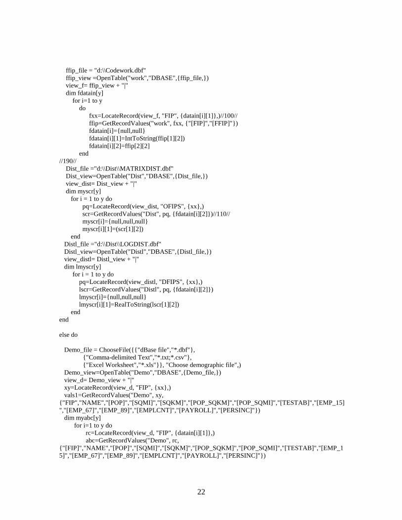
22

ffip_file = "d:\\Codework.dbf" ffip_view =OpenTable("work","DBASE",{ffip_file,}) view_f= ffip_view + "|" dim fdatain[y] for i=1 to y do fxx=LocateRecord(view_f, "FIP", {datain[i][1]},)//100// ffip=GetRecordValues("work", fxx, {"[FIP]","[FFIP]"}) fdatain[i]={null,null} fdatain[i][1]=IntToString(ffip[1][2]) fdatain[i][2]=ffip[2][2] end //190// Dist_file ="d:\\Dist\\MATRIXDIST.dbf" Dist_view=OpenTable("Dist","DBASE",{Dist_file,}) view_dist= Dist_view + "|" dim myscr[y] for i = 1 to y do pq=LocateRecord(view_dist, "OFIPS", {xx},) scr=GetRecordValues("Dist", pq, {fdatain[i][2]})//110// myscr[i]={null,null,null} myscr[i][1]=(scr[1][2]) end Distl_file ="d:\\Dist\\LOGDIST.dbf" Distl_view=OpenTable("Distl","DBASE",{Distl_file,}) view_distl= Distl_view + "|" dim lmyscr[y] for i = 1 to y do pq=LocateRecord(view_distl, "DFIPS", {xx},) lscr=GetRecordValues("Distl", pq, {fdatain[i][2]}) lmyscr[i]={null,null,null} lmyscr[i][1]=RealToString(lscr[1][2]) end end else do Demo_file = ChooseFile({{"dBase file","*.dbf"}, {"Comma-delimited Text","*.txt;*.csv"}, {"Excel Worksheet","*.xls"}}, "Choose demographic file",) Demo_view=OpenTable("Demo","DBASE",{Demo_file,}) view_d= Demo_view + "|" xy=LocateRecord(view_d, "FIP", {xx},) vals1=GetRecordValues("Demo", xy, {"FIP","NAME","[POP]","[SQMI]","[SQKM]","[POP_SQKM]","[POP_SQMI]","[TESTAB]","[EMP_15]","[EMP_67]","[EMP_89]","[EMPLCNT]","[PAYROLL]","[PERSINC]"}) dim myabc[y] for i=1 to y do rc=LocateRecord(view_d, "FIP", {datain[i][1]},) abc=GetRecordValues("Demo", rc, {"[FIP]","NAME","[POP]","[SQMI]","[SQKM]","[POP_SQKM]","[POP_SQMI]","[TESTAB]","[EMP_15]","[EMP_67]","[EMP_89]","[EMPLCNT]","[PAYROLL]","[PERSINC]"})

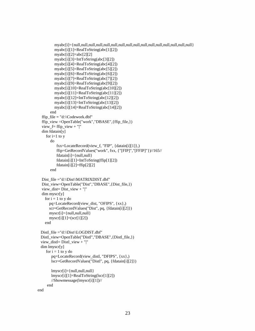
23

myabc[i]={null,null,null,null,null,null,null,null,null,null,null,null,null,null,null,null} myabc[i][1]=RealToString(abc[1][2]) myabc[i][2]=abc[2][2] myabc[i][3]=IntToString(abc[3][2]) myabc[i][4]=RealToString(abc[4][2]) myabc[i][5]=RealToString(abc[5][2]) myabc[i][6]=RealToString(abc[6][2]) myabc[i][7]=RealToString(abc[7][2]) myabc[i][9]=RealToString(abc[9][2]) myabc[i][10]=RealToString(abc[10][2]) myabc[i][11]=RealToString(abc[11][2]) myabc[i][12]=IntToString(abc[12][2]) myabc[i][13]=IntToString(abc[13][2]) myabc[i][14]=RealToString(abc[14][2]) end ffip_file = "d:\\Codework.dbf" ffip_view =OpenTable("work","DBASE",{ffip_file,}) view_f= ffip_view + "|" dim fdatain[y] for i=1 to y do fxx=LocateRecord(view_f, "FIP", {datain[i][1]},) ffip=GetRecordValues("work", fxx, {"[FIP]","[FFIP]"})//165// fdatain[i]={null,null} fdatain[i][1]=IntToString(ffip[1][2]) fdatain[i][2]=ffip[2][2] end Dist_file ="d:\\Dist\\MATRIXDIST.dbf" Dist_view=OpenTable("Dist","DBASE",{Dist_file,}) view_dist= Dist_view + "|" dim myscr[y] for i = 1 to y do pq=LocateRecord(view_dist, "OFIPS", {xx},) scr=GetRecordValues("Dist", pq, {fdatain[i][2]}) myscr[i]={null,null,null} myscr[i][1]=(scr[1][2]) end Distl_file ="d:\\Dist\\LOGDIST.dbf" Distl_view=OpenTable("Distl","DBASE",{Distl_file,}) view_distl= Distl_view + "|" dim lmyscr[y] for i = 1 to y do pq=LocateRecord(view_distl, "DFIPS", {xx},) lscr=GetRecordValues("Distl", pq, {fdatain[i][2]}) lmyscr[i]={null,null,null} lmyscr[i][1]=RealToString(lscr[1][2]) //Showmessage(lmyscr[i][1])// end end

24

dim b[2] b=runDbox("Default or User input model") if b="Yes" then do Coeff_file = "d:\\Coefficients\\Coefficient.dbf" Coeff_view=OpenTable("Coeff","DBASE",{Coeff_file,}) view_co= Coeff_view + "|" end else do Coeff_file = ChooseFile({{"dBase file","*.dbf"}, {"Comma-delimited Text","*.txt;*.csv"}, {"Excel Worksheet","*.xls"}}, "Choose coeff file",) Coeff_view=OpenTable("Coeff","DBASE",{Coeff_file,}) view_co= Coeff_view + "|" end reco = GetFirstRecord(view_co, {{"Constant", "null"}})//296// hi=GetRecordsValues(view_co, null, {"Constant","Distance","Log_Dist","Totalton","O_pop","D_pop","O_sqmi","D_sqmi","O_inc","D_inc","O_empcnt","D_empcnt","O_pay","D_pay","O_emp499","D_emp499","O_emp999","D_emp999","O_emp1k","D_emp1k"},null,y,,) //Assume 10 tons equals 1 truck load, and 120 tons equals 1 railcar load// trucks=10 rail=120 dim util[y] table_view=CreateTable("First","d:\\Trips\\Food & Related Products.dbf","DBASE", {{"ID","Integer",8,null,"No"},{"RailCars","Integer",8,null,"No"},{"TruckTrips","Integer",8,null,"No"}}) str=GetTableStructure(table_view) dim Ton_Rd[y] dim probrd[y] dim Ton_Rl[y] dim Trips_Rd[y] dim Trips_Rl[y] for i= 1 to y do if vals[i][3]<>0 then do util[i]=hi[1][1]+hi[2][1]*(myscr[i][1])/100+hi[3][1]*(Stringtoreal(lmyscr[i][1]))+(hi[4][1]*vals[i][3])/1000+ hi[5][1]*(vals1[3][2])/1000000+hi[6][1]*(StringToint(myabc[i][3]))/1000000+hi[7][1]*(vals1[4][2])/1000+hi[8][1]*(stringtoreal(myabc[i][4]))/1000+ hi[9][1]*(vals1[14][2])/1000000+hi[10][1]*(Stringtoreal(myabc[i][14]))/1000000+hi[11][1]*(vals1[12][2])/1000000+hi[12][1]*(stringtoint(myabc[i][12]))/1000000+ hi[13][1]*(vals1[13][2])/1000000+hi[14][1]*(stringtoint(myabc[i][13]))/1000000+hi[15][1]*(vals1[9][2])/10000+hi[16][1]*(stringtoreal(myabc[i][9]))/10000+ hi[17][1]*(vals1[10][2])/1000+hi[18][1]*(stringtoreal(myabc[i][10]))/1000+hi[19][1]*(vals1[11][2])/100+hi[20][1]*(stringtoreal(myabc[i][11]))/100 probrd[i]= 1/(1+exp(util[i]))

25

Ton_Rl[i]=(1-probrd[i])*vals[i][3] Ton_Rd[i]=(probrd[i])*vals[i][3] Trips_Rd[i]=R2I(Ton_Rd[i]/trucks)+1//because it rounds of to the lower integer level// Trips_Rl[i]=R2I(Ton_Rl[i]/rail)+1 end else do //Ton_Rl[i]=0.0000 //Ton_Rd[i]=0.0000 Trips_Rd[i]=0 Trips_Rl[i]=0 end rh=AddRecord(table_view,{{"ID",datain[i][1]},{"RailCars",Trips_Rl[i]},{"TruckTrips",Trips_Rd[i]}}) end dim util[y] table_view=CreateTable("Second","d:\\Trips\\Hazardous Materials.dbf","DBASE", {{"ID","Integer",8,null,"No"},{"RailCars","Integer",8,null,"No"},{"TruckTrips","Integer",8,null,"No"}}) str=GetTableStructure(table_view) dim Ton_Rd[y] dim probrd[y] dim Ton_Rl[y] dim Trips_Rd[y] dim Trips_Rl[y] for i=1 to y do if vals[i][4]<>0 then do util[i] =hi[1][2]+hi[2][2]*(myscr[i][1])/100+hi[3][2]*(Stringtoreal(lmyscr[i][1]))+(hi[4][2]*vals[i][4])/1000+ hi[5][2]*(vals1[3][2])/1000000+hi[6][2]*(StringToint(myabc[i][3]))/1000000+hi[7][2]*(vals1[4][2])/1000+hi[8][2]*(stringtoreal(myabc[i][4]))/1000+ hi[9][2]*(vals1[14][2])/1000000+hi[10][2]*(Stringtoreal(myabc[i][14]))/1000000+hi[11][2]*(vals1[12][2])/1000000+hi[12][2]*(stringtoint(myabc[i][12]))/1000000+ hi[13][2]*(vals1[13][2])/1000000+hi[14][2]*(stringtoint(myabc[i][13]))/1000000+hi[15][2]*(vals1[9][2])/10000+hi[16][2]*(stringtoreal(myabc[i][9]))/10000+ hi[17][2]*(vals1[10][2])/1000+hi[18][2]*(stringtoreal(myabc[i][10]))/1000+hi[19][2]*(vals1[11][2])/100+hi[20][2]*(stringtoreal(myabc[i][11]))/100 probrd[i]= 1/(1+exp(util[i]))//145// Ton_Rl[i]=(1-probrd[i])*vals[i][4] Ton_Rd[i]=(probrd[i])*vals[i][4] Trips_Rd[i]=R2I(Ton_Rd[i]/trucks)+1 Trips_Rl[i]=R2I(Ton_Rl[i]/rail)+1 end else do //Ton_Rl[i]=0.0000 //Ton_Rd[i]=0.0000 Trips_Rd[i]=0 Trips_Rl[i]=0 end rh=AddRecord(table_view,{{"ID",datain[i][1]},{"RailCars",Trips_Rl[i]},{"TruckTrips",Trips_Rd[i]}}) end

26

dim util[y] table_view=CreateTable("Third","d:\\Trips\\Construction Materials.dbf","DBASE", {{"ID","Integer",8,null,"No"},{"RailCars","Integer",8,null,"No"},{"TruckTrips","Integer",8,null,"No"}}) str=GetTableStructure(table_view) dim Ton_Rd[y] dim probrd[y] dim Ton_Rl[y] dim Trips_Rd[y] dim Trips_Rl[y] for i=1 to y do if vals[i][5]<>0 then do util[i] =hi[1][3]+hi[2][3]*(myscr[i][1])/100+hi[3][3]*(Stringtoreal(lmyscr[i][1]))+(hi[4][3]*(vals[i][5]))/1000+ hi[5][3]*(vals1[3][2])/1000000+hi[6][3]*(StringToint(myabc[i][3]))/1000000+hi[7][3]*(vals1[4][2])/1000+hi[8][3]*(stringtoreal(myabc[i][4]))/1000+ hi[9][3]*(vals1[14][2])/1000000+hi[10][3]*(Stringtoreal(myabc[i][14]))/1000000+hi[11][3]*(vals1[12][2])/1000000+hi[12][3]*(stringtoint(myabc[i][12]))/1000000+ hi[13][3]*(vals1[13][2])/1000000+hi[14][3]*(stringtoint(myabc[i][13]))/1000000+hi[15][3]*(vals1[9][2])/10000+hi[16][3]*(stringtoreal(myabc[i][9]))/10000+ hi[17][3]*(vals1[10][2])/1000+hi[18][3]*(stringtoreal(myabc[i][10]))/1000+hi[19][3]*(vals1[11][2])/100+hi[20][3]*(stringtoreal(myabc[i][11]))/100 probrd[i]= 1/(1+exp(util[i])) Ton_Rl[i]=(1-probrd[i])*vals[i][5] Ton_Rd[i]=(probrd[i])*vals[i][5] Trips_Rd[i]=R2I(Ton_Rd[i]/trucks)+1 Trips_Rl[i]=R2I(Ton_Rl[i]/rail)+1 end else do //Ton_Rl[i]=0.0000 //Ton_Rd[i]=0.0000 Trips_Rd[i]=0 Trips_Rl[i]=0 end rh=AddRecord(table_view,{{"ID",datain[i][1]},{"RailCars",Trips_Rl[i]},{"TruckTrips",Trips_Rd[i]}}) end dim util[y] table_view=CreateTable("Fourth","d:\\Trips\\Agricultural & Related Products.dbf","DBASE",{{"ID","Integer",8,null,"No"},{"RailCars","Integer",8,null,"No"},{"TruckTrips","Integer",8,null,"No"}}) str=GetTableStructure(table_view)//401// dim Ton_Rd[y] dim probrd[y] dim Ton_Rl[y] dim Trips_Rd[y] dim Trips_Rl[y] for i=1 to y do if vals[i][6]<>0

27

then do util[i] =hi[1][4]+hi[2][4]*(myscr[i][1])/100+hi[3][4]*(Stringtoreal(lmyscr[i][1]))+(hi[4][4]*(vals[i][6]))/1000+ hi[5][4]*(vals1[3][2])/1000000+hi[6][4]*(StringToint(myabc[i][3]))/1000000+hi[7][4]*(vals1[4][2])/1000+hi[8][4]*(stringtoreal(myabc[i][4]))/1000+ hi[9][4]*(vals1[14][2])/1000000+hi[10][4]*(Stringtoreal(myabc[i][14]))/1000000+hi[11][4]*(vals1[12][2])/1000000+hi[12][4]*(stringtoint(myabc[i][12]))/1000000+ hi[13][4]*(vals1[13][2])/1000000+hi[14][4]*(stringtoint(myabc[i][13]))/1000000+hi[15][4]*(vals1[9][2])/10000+hi[16][4]*(stringtoreal(myabc[i][9]))/10000+ hi[17][4]*(vals1[10][2])/1000+hi[18][4]*(stringtoreal(myabc[i][10]))/1000+hi[19][4]*(vals1[11][2])/100+hi[20][4]*(stringtoreal(myabc[i][11]))/100 probrd[i]= 1/(1+exp(util[i])) Ton_Rl[i]=(1-probrd[i])*vals[i][6] Ton_Rd[i]=(probrd[i])*vals[i][6] Trips_Rd[i]=R2I(Ton_Rd[i]/trucks)+1 Trips_Rl[i]=R2I(Ton_Rl[i]/rail)+1 end else do //Ton_Rl[i]=0.0000 //Ton_Rd[i]=0.0000 Trips_Rd[i]=0 Trips_Rl[i]=0 end rh=AddRecord(table_view,{{"ID",datain[i][1]},{"RailCars",Trips_Rl[i]},{"TruckTrips",Trips_Rd[i]}}) end dim util[y] table_view=CreateTable("Fifth","d:\\Trips\\Manufacturing Products.dbf","DBASE",{{"ID","Integer",8,null,"No"},{"RailCars","Integer",8,null,"No"},{"TruckTrips","Integer",8,null,"No"}}) str=GetTableStructure(table_view) dim Ton_Rd[y] dim probrd[y] dim Ton_Rl[y] dim Trips_Rd[y] dim Trips_Rl[y] for i=1 to y do if vals[i][7]<>0 then do util[i] =hi[1][5]+hi[2][5]*(myscr[i][1])/100+hi[3][5]*(Stringtoreal(lmyscr[i][1]))+(hi[4][5]*(vals[i][7]))/1000+ hi[5][5]*(vals1[3][2])/1000000+hi[6][5]*(StringToint(myabc[i][3]))/1000000+hi[7][5]*(vals1[4][2])/1000+hi[8][5]*(stringtoreal(myabc[i][4]))/1000+ hi[9][5]*(vals1[14][2])/1000000+hi[10][5]*(Stringtoreal(myabc[i][14]))/1000000+hi[11][5]*(vals1[12][2])/1000000+hi[12][5]*(stringtoint(myabc[i][12]))/1000000+ hi[13][5]*(vals1[13][2])/1000000+hi[14][5]*(stringtoint(myabc[i][13]))/1000000+hi[15][5]*(vals1[9][2])/10000+hi[16][5]*(stringtoreal(myabc[i][9]))/10000+ hi[17][5]*(vals1[10][2])/1000+hi[18][5]*(stringtoreal(myabc[i][10]))/1000+hi[19][5]*(vals1[11][2])/100+hi[20][5]*(stringtoreal(myabc[i][11]))/100 probrd[i]= 1/(1+exp(util[i]))//438// Ton_Rl[i]=(1-probrd[i])*vals[i][7]

28

Ton_Rd[i]=(probrd[i])*vals[i][7] Trips_Rd[i]=R2I(Ton_Rd[i]/trucks)+1 Trips_Rl[i]=R2I(Ton_Rl[i]/rail)+1 end else do //Ton_Rl[i]=0.0000 //Ton_Rd[i]=0.0000 Trips_Rd[i]=0 Trips_Rl[i]=0 end rh=AddRecord(table_view,{{"ID",datain[i][1]},{"RailCars",Trips_Rl[i]},{"TruckTrips",Trips_Rd[i]}}) end dim util[y] table_view=CreateTable("Sixth","d:\\Trips\\Machinery & Equipment.dbf","DBASE",{{"ID","Integer",8,null,"No"},{"RailCars","Integer",8,null,"No"},{"TruckTrips","Integer",8,null,"No"}}) str=GetTableStructure(table_view) dim Ton_Rd[y] dim probrl[y] dim Ton_Rl[y] dim Trips_Rd[y] dim Trips_Rl[y] for i=1 to y do if vals[i][8]<>0 then do probrl[i]= 1.0000 Ton_Rl[i]=1.0000*vals[i][8] Ton_Rd[i]=0.0000 Trips_Rd[i]=R2I(Ton_Rd[i]/trucks) Trips_Rl[i]=R2I(Ton_Rl[i]/rail)+1 end else do //Ton_Rl[i]=0.0000 //Ton_Rd[i]=0.0000 Trips_Rd[i]=0 Trips_Rl[i]=0 end rh=AddRecord(table_view,{{"ID",datain[i][1]},{"RailCars",Trips_Rl[i]},{"TruckTrips",Trips_Rd[i]}}) end dim util[y] table_view=CreateTable("Seventh","d:\\Trips\\Mixed Freight Shipments.dbf","DBASE",{{"ID","Integer",8,null,"No"},{"RailCars","Integer",8,null,"No"},{"TruckTrips","Integer",8,null,"No"}}) str=GetTableStructure(table_view) dim Ton_Rd[y] dim probrl[y] dim Ton_Rl[y] dim Trips_Rd[y] dim Trips_Rl[y] for i=1 to y

29

do if vals[i][9]<>0 then do probrl[i]= 1.0000 Ton_Rl[i]=1.0000*vals[i][9] Ton_Rd[i]=0.0000 Trips_Rd[i]=R2I(Ton_Rd[i]/trucks) Trips_Rl[i]=R2I(Ton_Rl[i]/rail)+1 end else do //Ton_Rl[i]=0.0000 //Ton_Rd[i]=0.0000 Trips_Rd[i]=0 Trips_Rl[i]=0 end rh=AddRecord(table_view,{{"ID",datain[i][1]},{"RailCars",Trips_Rl[i]},{"TruckTrips",Trips_Rd[i]}}) end table_view=CreateTable("Mark","d:\\Trips\\Markets.dbf","DBASE",{{"ID","Integer",8,null,"No"},{"Origin","String",16,null,"Yes"},{"Market","String",12,null,"Yes"}}) str=GetTableStructure(table_view) for i=1 to y do rh=AddRecord(table_view,{{"ID",datain[i][1]},{"Origin",vals[i][1]},{"Market",vals[i][2]}}) end //new starts// food_file="d:\\Trips\\Food & Related Products.dbf" food_view=OpenTable("First","DBASE",{food_file,}) view_f=food_view+"|" dim a[y] dim b[y] dim c[y] for i=1 to y do a=LocateRecord(view_f,"ID",{datain[i][1]},) b=GetRecordValues("First",a,{"[RailCars]","[TruckTrips]"}) c[i]={null,null} c[i][1]=b[1][2] c[i][2]=b[2][2] end haz_file="d:\\Trips\\Hazardous Materials.dbf" haz_view=OpenTable("Second","DBASE",{haz_file,}) view_h=haz_view+"|" dim d[y] dim e[y] dim f[y] for i=1 to y do d=LocateRecord(view_h,"ID",{datain[i][1]},) e=GetRecordValues("Second",d,{"[RailCars]","[TruckTrips]"}) f[i]={null,null} f[i][1]=e[1][2] f[i][2]=e[2][2] end

30

const_file="d:\\Trips\\Construction Materials.dbf" const_view=OpenTable("Third","DBASE",{const_file,}) view_c=const_view+"|" dim g[y] dim h[y] dim j[y] for i=1 to y do g=LocateRecord(view_c,"ID",{datain[i][1]},) h=GetRecordValues("Third",g,{"[RailCars]","[TruckTrips]"}) j[i]={null,null} j[i][1]=h[1][2] j[i][2]=h[2][2] end agri_file="d:\\Trips\\Agricultural & Related Products.dbf" agri_view=OpenTable("Fourth","DBASE",{agri_file,}) view_a=agri_view+"|" dim k[y] dim l[y] dim m[y] for i=1 to y do k=LocateRecord(view_a,"ID",{datain[i][1]},) l=GetRecordValues("Fourth",k,{"[RailCars]","[TruckTrips]"}) m[i]={null,null} m[i][1]=l[1][2] m[i][2]=l[2][2] end mfg_file="d:\\Trips\\Manufacturing Products.dbf" mfg_view=OpenTable("Fifth","DBASE",{mfg_file,}) view_mfg=mfg_view+"|" dim n[y] dim o[y] dim p[y] for i=1 to y do n=LocateRecord(view_mfg,"ID",{datain[i][1]},) o=GetRecordValues("Fifth",n,{"[RailCars]","[TruckTrips]"}) p[i]={null,null} p[i][1]=o[1][2] p[i][2]=o[2][2] end mach_file="d:\\Trips\\Machinery & Equipment.dbf" mach_view=OpenTable("Sixth","DBASE",{mach_file,}) view_mach=mach_view+"|" dim q[y] dim r[y] dim s[y] for i=1 to y do q=LocateRecord(view_mach,"ID",{datain[i][1]},) r=GetRecordValues("Sixth",q,{"[RailCars]","[TruckTrips]"}) s[i]={null,null}

31

s[i][1]=r[1][2] s[i][2]=r[2][2] end mix_file="d:\\Trips\\Mixed Freight Shipments.dbf" mix_view=OpenTable("Seventh","DBASE",{mix_file,}) view_mix=mix_view+"|" dim t[y] dim u[y] dim v[y] for i=1 to y do t=LocateRecord(view_mach,"ID",{datain[i][1]},) u=GetRecordValues("Seventh",t,{"[RailCars]","[TruckTrips]"}) v[i]={null,null} v[i][1]=u[1][2] v[i][2]=u[2][2] end new_table=CreateTable("New","d:\\Trips\\Total","DBASE",{{"RouteID","Integer",8,null,"No"},{"ID","Integer",8,null,"No"},{"RailCars","Integer",8,null,"No"},{"TruckTrips","Integer",8,null,"No"}}) str=GetTableStructure(new_table) dim new[y] for i=1 to y do new[i]={null,null} new[i][1]=c[i][1]+f[i][1]+j[i][1]+m[i][1]+p[i][1]+s[i][1]+v[i][1] new[i][2]=c[i][2]+f[i][2]+j[i][2]+m[i][2]+p[i][2]+s[i][2]+v[i][2] add=AddRecord(new_table,{{"RouteID",i},{"ID",datain[i][1]},{"RailCars",new[i][1]},{"TruckTrips",new[i][2]}}) end RunMacro("G30 File Close All") CopyDatabase("d:\\Texas Counties_fips","d:\\Trips\\geo.dbd") mp1=OpenMap("d:\\texascntys.map", { {"Menu", "My System Menu"}, {"Toolbar", "My own custom toolbar"}, {"Auto Project", "True"}}) Setlayer("Texas Counties") a=Getmap() mp2 = CreateMap("Texas", { {"Scope", GetLayerScope("Texas Counties") }, {"Menu", "My System Menu"}, {"Toolbar", "My own custom toolbar"}, {"Auto Project", "True"} }) //Closemap(a) geo_file = "d:\\Trips\\geo.dbd" lyrs = GetDBLayers(geo_file) new_lyr = AddLayer("Texas", "Counties", geo_file, lyrs[1])

32

Savemap("Texas","d:\\Trips\\new.map") closemap() mp1=OpenMap("d:\\Trips\\new.map", { {"Menu", "My System Menu"}, {"Toolbar", "My own custom toolbar"}, {"Auto Project", "True"}}) Setlayer("Counties") Code_file = "d:\\Portinfo.dbf" Code_view =OpenTable("Code","DBASE",{Code_file,}) view_c= Code_view + "|" cab=LocateRecord(view_c, "Port", {vals[1][1]},) cabl=GetRecordValues("Code", cab, {"Port","[FIP]","NAME"}) SelectByIDs("Origin","More", {cabl[2][2]}) for i=1 to y do SelectByIDs("Destinations","More",{datain[i][1]}) end SetDisplayStatus("Origin", "Active") SetDisplayStatus("Destinations", "Active") SetFillColor("Origin", ColorRGB(0, 0, 0)) SetFillColor("Destinations", ColorRGB(0, 0, 65535)) redrawmap() Open = OpenTable("New", "DBASE", {"d:\\Trips\\Total.dbf",}) info = GetViewTableInfo("New") //showarray(info) JoinTableToLayer("d:\\Trips\\geo.dbd","Texas Counties", "DBASE","D:\\Trips\\Total.dbf" ,, "ID",) SaveMap(, "d:\\Trips\\modesplit.map") b=Getmap() //Showmessage(b) closemap(b) CopyDatabase("d:\\Modified Texas Roads","d:\\Trips\\highways.dbd") mp1=OpenMap("d:\\newmap.map", { {"Menu", "My System Menu"}, {"Toolbar", "My own custom toolbar"}, {"Auto Project", "True"}}) c=Getmap() //Showmessage(b) mp2 = CreateMap("Texasroads", { {"Scope", GetLayerScope("NA Highway") }, {"Menu", "My System Menu"}, {"Toolbar", "My own custom toolbar"}, {"Auto Project", "True"} }) geo_file = "d:\\Trips\\highways.dbd" lyrs = GetDBLayers(geo_file) //Showarray(lyrs) new_lyra= AddLayer("Texasroads", "Xsection", geo_file, lyrs[1])

33

new_lyra = AddLayer("Texasroads", "Highway",geo_file, lyrs[2]) //Showmessage(new_lyra) //Showmessage(new_lyrb) Savemap(,"d:\\Trips\\roads.map") info = CreateRouteSystem("d:\\Trips\\goodroute", "d:\\Trips\\highways.dbd", "NA Highway",{{"Binary Tables","True"},{"Label","Routes"},{"Links Table","Complete",,},{"Name","CreatedRoutes"},{"Routes Table","False",{{"Operator", "S", 30, 0, "False"}}},{"Stops","Stops",}}) layer_name = info[1] path = info[2] //Showmessage("next is layer name") //Showmessage(layer_name) //Showmessage(path) //Showmessage("routesystem created") //on escape default actual_lyr_name = AddRouteSystemLayer("Texasroads", "abcd", "d:\\Trips\\goodroute.rts",) //Showmessage("added") net_handle = ReadNetwork("d:\\roadnetwork") n_nodes = NetworkNodes(net_handle) n_links = NetworkLinks(net_handle) //Showmessage("done") Setlayer("NA Highway Xsection") //Showmessage("Layer Set") id_file="d:\\xsection.dbf" id_view=OpenTable("xid","DBASE",{id_file,}) view_id=id_view +"|" abc=LocateRecord(view_id,"ID",{cabl[2][2]},) def=GetRecordValues("xid",abc,{"[ID]","[XID]"}) SelectByIDs("Origin","More",{def[2][2]}) for i=1 to y do xy=LocateRecord(view_id,"ID",{datain[i][1]},) yz=GetRecordValues("xid",xy,{"[ID]","[XID]"}) SelectByIDs("Destinations","More",{yz[2][2]}) end //Showmessage("selected") //SetDisplayStatus("Origin","Active") //SetDisplayStatus("Destinations","Active") //showmessage("displayset") //SetFillColor("Origin", ColorRGB(0, 0, 65535)) //SetFillColor("Destinations", ColorRGB(0, 0, 0)) pqr=AddShortestPathRoutes(net_handle, "abcd", "NA Highway Xsection|Origin", "NA Highway Xsection|Destinations", , , {{"Node ID","NA Highway Xsection.ID"},{,}}) new_table=CreateTable("Links","d:\\Trips\\Links","DBASE",{{"RouteID","Integer",8,null,"No"},{"LinkID","Integer",8,null,"No"},{"TruckTrips","Integer",8,null,"No"}}) str=GetTableStructure(new_table) dim names[y] dim ids[y] dim c[y] dim abc[y]

34

dim b[y] for i=1 to y do names = GetRouteNames("abcd") // Showmessage(names[i]) ids = GetRouteIDs("abcd", {names[i]}) c[i]=ids[1] //Showmessage(I2S(c[i])) a = GetRouteLinks("abcd", names[i]) abc= ArrayLength(a) b[i]=abc x=b[i] //ShowMessage(I2S(x)) a = GetRouteLinks("abcd", names[i]) // ShowArray(a) for k=1 to x do //Showmessage(I2S(a[k][1])) add=AddRecord(new_table,{{"RouteID",c[i]},{"LinkID",a[k][1]},{"TruckTrips",new[i][2]}}) end end first_file ="d:\\Trips\\Links.dbf" first_view=OpenTable("Links","DBASE",{first_file,}) view_first= first_view + "|" rslt = AggregateTable("See","Links|","DBASE","d:\\Trips\\See","LinkID",{{"TruckTrips","sum", }, {"TruckTrips","min", }, {"TruckTrips","max", }, {"TruckTrips","average",}} ,null) //Showmessage("Firststepfine") view1= OpenTable("See", "DBASE", {"d:\\Trips\\See.dbf",}) num=Getrecordcount("See",null) // //ShowMessage(I2S(num)) z=num view_info = GetViews() //Showarray(view_info) view=view1 + "|" rh = GetFirstRecord(view,{{"LinkID","null"}}) values = GetRecordsValues(view,null,{"[LinkID]","[TruckTrips]"},null,z,,) //Showarray(values) //Showmessage(I2S(values[1][2])) //Showmessage(R2S(values[2][2])) //for i=1 to 10 do //Showmessage(I2S(values[1][i])) //Showmessage(R2S(values[2][i])) //end latest_table=CreateTable("Sum_1","d:\\Sum_1","DBASE",{{"LinkID","Integer",8,null,"No"},{"TruckTrips","Integer",8,null,"No"}}) for i=1 to z do add_rec=AddRecord(latest_table,{{"LinkID",values[1][i]},{"Trucktrips",values[2][i]}}) end Open = OpenTable("Sum_1", "DBASE", {"d:\\Sum_1.dbf",})

35

info_array = GetViewTableInfo("Sum_1") JoinTableToLayer("d:\\Trips\\highways.dbd","NA Highway", "DBASE","d:\\Sum_1.dbf" ,, "LinkID",) SetLayer("Highway") SaveMap(, "d:\\Trips\\Path.map") Showmessage("Close") maps = GetMapNames() for i = 1 to maps.length do CloseMap(maps[i]) end Endmacro Dbox"Default or New",,50,8 init do str="Do you want to use default demographic dataset?" enditem text 5,1,40,4 variable:str align:center button "Yes" 10,5,5 default do return ("Yes") enditem button "No" 33,5,7 do return ("No") enditem endDbox Dbox"Default or User input model",,50,8 init do ShowMessage("The default model has the following variables - Distance,Logdistance,Tonnage,OriginPopulation,DestinationPopulation,OriginIncome,DestinationIncome,OriginPayroll,DestinationPayroll") str="Do you want to use the default modal split model?" enditem text 5,1,40,4 variable:str align:center button "Yes" 10,5,5 default do return ("Yes") enditem button "No" 33,5,7 do return ("No") enditem endDbox Dbox "Exit" ,,50,8 Toolbox init do Showmessage("Exit") enditem endDbox

36

37

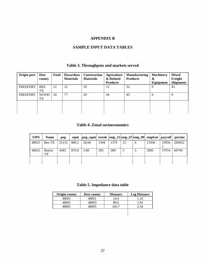
APPENDIX B

SAMPLE INPUT DATA TABLES

Table 3. Throughputs and markets served

Origin port Dest county

Food Hazardous Materials

Construction Materials

Agriculture & Related Products

Manufacturing Products

Machinery & Equipment

Mixed Freight Shipments

FREEPORT BEE TX

12 12 10 12 32 0 43

FREEPORT WOOD TX

34 77 20 34 43 0 0

Table 4. Zonal socioeconomics

Table 5. Impedance data table

Origin county Dest county Distance Log Distance 48001 48001 14.4 1.16 48001 48003 80.6 1.91 48001 48005 343.7 2.54

FIPS Name pop sqmi pop_sqmi testab emp_15 emp_67 emp_89 emplcnt payroll persinc

48025 Bee TX 25135 880.2 28.60 1394 1379 15 0 11930 199561

284952

48023 Baylor TX

4385 870.8 5.00 395 389 3 3 3985 37974 69740

38

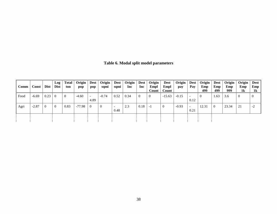
Table 6. Modal split model parameters

Comm

Const

Dist

Log Dist

Total ton

Origin pop

Dest pop

Origin sqmi

Dest sqmi

Origin Inc

Dest Inc

Origin Empl Count

Dest Empl Count

Origin pay

Dest Pay

Origin Emp 499

Dest Emp 499

Origin Emp 999

Origin Emp 1k

Dest Emp 1k

Food -6.69 0.23 0 0 -4.60 -4.89

-0.74 0.52 0.34 0 0 -15.63 -0.15 -0.12

0 1.63 3.6 0 0

Agri -2.87 0 0 0.83 -77.98 0 0 -0.48

2.3 0.18 -1 0 -0.93 -0.21

12.31 0 23.34 21 -2