Freie Universität Berlin Department of Physics GPII Basic ... · Freie Universität Berlin Department of Physics Basic Laboratory Course in Physics ... and conducting an experiment

Freie Universität Berlin Department of Physics Basic Laboratory Course in Physics

GPII Two Semester basic laboratory course for students of Physics, Geophysics, Meteorology and for Teacher Candidates with physics as first or second subject.

Two Semester basic laboratory course for students of Physics, Geophysics, Meteorology and for Teacher Candidates with physics as first or second major.

Aim of the Laboratory Course Introduction to the fundamental techniques of quantitative ex-perimental- and scientific methods in physics (measurement methods, measurement techniques, documentation, mathe-matical-statistical und practical evaluation methods / error cal-culations, critical discussion and scientific conclusion, written report and presentation). Dealing with selected topics in physics in a deeper and complementary way.

Core Rules

Preparation based on lectures and text books according to information contained in the script.

The experiments begin c.t. and students arriving more than 15 minutes later will be excluded from taking part.

The two page introduction (intended as part of the experi-mental report) is to be presented at the beginning of the experiment.

The tutor introduces the students to the experiment and makes sure that they are sufficiently prepared and if not, whether the work should be repeated at a later date.

The experiment and documentation of the results is made as quick as possible under the guidance of the tutor, whereby, time for further discussions of the physical back-ground should be taken into account.

Evaluation of the experiment by means of tables and graphs takes place after about 3 hours with the help of the tutor. Thereafter, further work is to be done on the report (protocol).

The 4 hours are to be fully used to complete the protocol and can then only be cut short when the tutor hands out an attestation.

The total number of experiments (as a rule 11) must be completed within the laboratory course, whereby a maxi-mum of 2 experiments can be repeated at the end of the course.

Attestations for all experiments must be noted at the latest on the last day of the course, otherwise the course can not be assessed and becomes invalid.

Integration with the Physics Curricula Two laboratory courses (GP I and II) are scheduled after the respective lecture courses (Physics I and II). Restrictions with respect to the contents of the lectures are unavoidable due to the timescale and the placement of the laboratory course. This is especially evident for students taking part in the vacation la-boratory courses where subjects must be handled in advance without prior lecture material (Optics, Atomic Physics Quantum Phenomena).

Organization Semester Course (weakly, 4 h) and Vacation Course (4 weeks, 12 h per week). Laboratory course in small groups. Pairs of students performing and evaluating an experiment. A tutor assists a group of 3 pairs on the same or related experiments. Good preparation before the experiment is important. A two page introduction to the sub-ject matter is handed out before each experiment and is in-tended as part of the evaluation . Course Schedule with Experimental Work, Evaluation and (as a rule) start of the written report (protocol). Work on the two page introduction to the subject matter (pre-pared beforehand), presentation of the experimental findings with summary and critical discussion of the results. Course Material: Description of the experiment (script) contain-ing information on the relevant physics, experimental set-up and the tasks to be performed. Report book for the written ex-perimental protocol – to be bought by the student.

Evaluation Experimental certificate with grades according to ECTS (Euro-pean Credit Transfer System). Point system for the individual experiments. No tests or final seminar.

Experiments Experiments with various grades of difficulty from simple exper-iments in GP I, to give a basic feeling for the methods involved in experimental physics, to experiments with deeper physical background, which, for a fuller understanding, require higher lecture courses in physics.

Note A sensitive indicator for physical understanding is the applica-tion of gained knowledge. The physical principles and the con-nections between phenomena should be demonstrated by deal-ing with the problems involved and by critical observation. As a part of scientific training, it is not the intention of the labor-atory course to only impart „mechanical knowledge“ but it should lead to scientific thinking, i.e., answering questions of a physical nature or drawing conclusions from findings and laws through critical discussions in small groups and final evaluation of the observations and quantitative results. Edition: 22.12.006 Revision: Rentzsch

BASIC LABORATORY COURSE IN PHYSICS

Introduction to the fundamental techniques of quantitative ex-perimental- and scientific methods in physics: Measurement methods, measurement techniques, documentation, mathe-matical-statistical und practical evaluation methods (error cal-culations), critical discussion and scientific conclusion, written

GP POINT SYSTEM -3-

report and presentation. Dealing with selected topics in physics in a deeper and complementary way.

Two laboratory courses (GP I and II) scheduled after the lecture courses Physics I and II, however, with reference to the com-plete material handled in lecture courses Physics I-IV.

Experiments and reports done in team work consisting of a group of 6 (3 pairs) under the assistance of a tutor.

Completion of introductory reports on the subject matter and physical background, presentation of the experimental findings with a summary and critical discussion of the results as an ex-ercise in scientific writing.

Introductory text books provided the basic knowledge in a clear and connected manner, but only in passing, mention the way to the working methods of physics. Physical knowledge comes about either through quantitative observation of the natural pro-cesses, i.e., by means of experiments or by mathematical for-mulations of physical phenomena – theoretical work.

Laboratory courses give a feeling for the experimental methods of physics. The aim of the basic course is to introduce the stu-dents to elementary experimental and scientific working meth-ods and critical quantitative thinking. This includes setting-up and conducting an experiment (measurement techniques and methods), documentation, evaluation (error calculations), dis-cussion of the findings and scientific conclusions and finally presentation of the written report.

The basic course intentionally places the scientific method in the foreground. The physical questions presented in the course have long been answered, and the experiments are to be un-derstood as providing classical examples for methods and tech-niques which recur in current research. Yet physics is always behind the work and does not differentiate between simple and difficult. It is the physicist, whether “professional” or in training, who asks the questions and thus determines the standard.

The laboratory course allows the student to tackle the work in an individual way so that the learning process is strongly self determined. Elementary and important prerequisites are curios-ity and the ambition to understand.

Error Calculat ions

A fundamental phenomena of experimental work is the fact that the evaluation of natural processes is never absolute and all results must be considered as approximate. As a consequence, the empirical experimental data must be handled statistically in the form of error calculations.

An important aspect of the laboratory course is to introduce the student to the basic methods of error calculations. The first

steps and basic exercises in error calculations are found in An-nex I of this script (under the heading „ERROR CALCULA-TIONS”). (Practical exercises in error calculations will be given out before the laboratory course begins and must be handed in at the date of the first experiment). Learning the skills of error calculations is then the aim of the subsequent experimental work.



Topics and Experiments

The topics of the laboratory course are coordinated with the contents of the lecture course. The experiments range from simple to demanding.

In some cases, due to organizational problems (especially in vacation courses), the topics handled in the experiments have not yet been discussed in the lectures. This requires intensive self-preparation by the student.

Preparat ion

Successful experimental work requires good physical- and mathematical preparation using text books and the experi-mental script. The laboratory course has the specific aim of deepening ones knowledge of physical processes and must be seen as complementary to the material handled in lectures and work done in tutorial exercises.

Repor t

The written reports serve not only as proof of experimental work but also as an exercise in the method of scientific writing. Con-tents and form must be such that the interested reader is intro-duced to the topic and the questions to be answered in an effi-cient and concise way and is able to follow and understand the work and conclusions. This aspect must be kept in mind and it should not be limited to a mere presentation of measured data and calculations.

Rules of the Laboratory Course

Laboratory Report Book

Laboratory regulations require that all experimental work from description to data recording and evaluation be presented in bound exercise books. Please bring suitable books (DINA4-chequered, no ring bound books) to the course. You should buy 2 – 3 books. Work done on loose or tacked paper leads to un-certainty as to its origin or loss of pages i.e. data.

Additional pages (e.g. graph paper) must be glued to a thin strip of the inside edge of a book page so that both sides of the ad-ditional page can be used. Attaching pages with paper clips is not permitted.

Graph Paper

Graphs must be drawn on graph paper (mm paper, log-paper; available in the laboratory).

Written Preparation

A written introduction to the topic and experimental task (as part of the report) must be presented before beginning the experi-ment. This must be prepared by each student. Since, as a rule, one of the report books of a pair of students is in the hands of the tutor for correction, the affected student must write the in-troduction on loose paper and later glue it into his/her report book.

The students must be able prove that they have prepared the work through discussions with the tutor.

Insufficiently prepared students will not be permitted to take part in the experiment. The experiment is noted as failed and must be repeated at a later date. If a student is rejected because of insufficient preparation, a colloquium can be set up by the head of the course to test the student. (The rules stipulate that no more than 2 failures are allowed).

Times of the Laboratory Course

The courses begin punctually at 9.15 or 14.15 h.

33/4 hours (9.15-13 h and 14.15-18 h respectively) are set for the work. After the experiment is completed, the remaining time is used to evaluate important parts of the data under the direc-tion of the tutor (e.g., graphical presentations).

Structure and Form of the Report

The report is structured in two sections: Experimental documen-tation (measurement protocol) and the presentation (basic the-ory, evaluation, conclusion and discussion). The form is such

that an interested reader can follow and understand the con-tents, results and conclusions (and allows the tutor to make cor-rections in a reasonable time).

The measurement protocol must be hand written and checked by the tutor for completeness and correctness. Thereafter the tutor gives an attestation. Measurement protocols without attes-tation will not be recognized.

Handing Over the Report

The reports should be started during the respective experiment and must be handed over at the date of the next experiment.

Failure to hand over the report punctually leads to exclusion from the next experiment.

Missing- and Failed Experiments

If a student misses or is expelled from an experiment then his/her partner must complete the experiment alone.

The excluded partner must repeat the experiment on his/her own at a later date. (The date is set by the head of the laboratory course).

Working in Partnership

Normally students work in pairs, so that each is dependent on other. Work in conjunction with your partner and discuss each experiment so that no problems occur in completing the report and the handing out of attestations.

Attestations; Handing Out the Course Certificates

The handing out of the course certificates only t - 3 -akes place after presenting the complete attestations. Attestations can only be given by the responsible tutor.

Point System Each experiment is graded according to a point system. At the end of the course, the summed points serve to measure the to-tal performance according to the rules of the ECTS (European Credit Transfer System).

GP POINT SYSTEM -3-

The grading is given in % of the maximum number of points.

[100% – 81%] = A (very good) [ 80% – 61%] = B (good) [ 60% – 41%] = C (satisfactory) [ 40% – 27%] = D (sufficient) [ – 27%] = E (fail)

Each experiment is individually graded, whereby a maximum of 5 points can be given. The performance points for each experi-ment corresponds to the ETCS grades. 5 - 4.3 points = A (very good) 4 - 3.3 points = B (good) 3 - 2.3 points = C (satisfactory) 2 - 1.0 points = D (satisfactory) < 1.0 point = E (sufficient) (successful completion of an experiment requires, as a mini-mum, a grade of 1 point). The assessment of the work done is based on the following cat-egories:

A: Basic knowledge and understanding of the physics in-volved, preparing for the experiment.

B: Experimental ability (practical and methodical work and evaluation).

C: Scientific discussion and report (evaluating the experiment and the results, written report).

The points are noted on the group cards, report book, attesta-tion certificates and the file cards by the tutor.

CONTENTS GP II

General Information

Aim of the Laboratory Course 1 Rules of the Laboratory Course 4 Point System 4 Report 5

Model Report 6 Standard Text Books 12

Experiments

MIK Microscope 14 OPS Optical Spectroscopy 18 BEU Diffraction and Interference 25 FAP Fabry-Perot Etalon 29 SPL Specific Charge of the Electron 33 MLK Millikan Experiment 36 FHZ Franck-Hertz Experiment 39 PHO Photo Emission 42 IND Induction 45 WSK Alternating Current Circuits 49 HAL Hall Effect 53 TRA Transistor 56

Annex

Annex I Error Calculations 60

Annex II He-Ne Laser 62

Annex III Current Conduction 64

Annex IV Alternating Current Operators 67

Annex V Transistors 67



REPORT GPII

The report serves as an exercise in scientific writing and presentation. It should, on the one hand, be complete and on the other concise and efficient. As an orientation, refer to the model report below.

The report consists of a measurement protocol and elabora-tion:

The measurement protocol is a documentation of the ex-perimental procedure.

It must contain all information with respect to experimental set-up, data and observations from which one can com-pletely understand and evaluate the experiment even af-ter the equipment is dismantled.

Elaboration refers to presentation and communication.

It contains a short presentation of the basic physics in-volved and the question posed, evaluation, summary and critical discussion of the results and the scientific conclu-sions.

One of the most important aspects of a written report is its or-ganization, i.e., how it is structured. The following describes a standard structure obligatory for the laboratory reports.

Measurement Protocol

The measurement protocol is structured as follows:

Title (Experimental Topic)

Name; Date

Names of the students carrying out the experiment and of the tutor; date the experiment was done.

Experimental Set-Up and Equipment

Drawing of the set-up; list of the equipment used and equipment data.

Measured Values

Values with dimensions and units, error limits. Commen-tary on the error estimates. Data in the form of tables.

Other Observations.

Elaboration

The elaboration must also be handwritten in the report book (machine written sections or formulae are glued onto the pages of the report). The elaboration is structured as follows:

Title

(Experimental topic; name of the authors and the tutor; date of the elaboration)

Basic Physics

A concise presentation of the basic physics with respect to the topic and the questions involved, the measurement method and the equations (copying directly from the liter-ature is not allowed).

The presentation must give a short but complete overview of the essential aspects of the physical quantities studied and the laws governing them. It is not required to go into details as found in text books.

A description of the practical experimental methods is out of place here.

Evaluation

A presentation of the evaluation in graphical form (on graph paper glued onto the appropriate page of the text), evaluated parameters, intermediate results, final results and error limits. Error discussion.

The derivation of the results must be simple to understand and check (no scribbled notes).

Summary and Discussion of the Results

Concise Presentation:

What was measured and how the measurements were made?

GP MODEL REPORT 12-

(1) MODEL REPORT GPII

(2)

(3) (4)

(5)

(6)

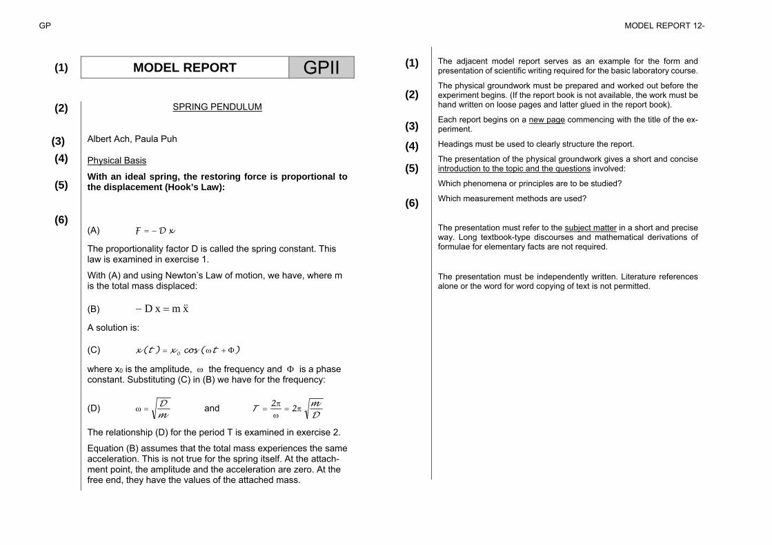
SPRING PENDULUM

Albert Ach, Paula Puh

Physical Basis

With an ideal spring, the restoring force is proportional to the displacement (Hook’s Law):

(A) xD F

The proportionality factor D is called the spring constant. This law is examined in exercise 1.

With (A) and using Newton’s Law of motion, we have, where m is the total mass displaced:

(B) xmxD

A solution is:

(C) )(cos)( 0 txtx

where x0 is the amplitude, the frequency and is a phase constant. Substituting (C) in (B) we have for the frequency:

(D) mD

and DmT

22

The relationship (D) for the period T is examined in exercise 2.

Equation (B) assumes that the total mass experiences the same acceleration. This is not true for the spring itself. At the attach-ment point, the amplitude and the acceleration are zero. At the free end, they have the values of the attached mass.

(1)

(2)

(3)

(4)

(5)

(6)

The adjacent model report serves as an example for the form and presentation of scientific writing required for the basic laboratory course.

The physical groundwork must be prepared and worked out before the experiment begins. (If the report book is not available, the work must be hand written on loose pages and latter glued in the report book).

Each report begins on a new page commencing with the title of the ex-periment.

Headings must be used to clearly structure the report.

The presentation of the physical groundwork gives a short and concise introduction to the topic and the questions involved:

Which phenomena or principles are to be studied?

Which measurement methods are used?

The presentation must refer to the subject matter in a short and precise way. Long textbook-type discourses and mathematical derivations of formulae for elementary facts are not required.

The presentation must be independently written. Literature references alone or the word for word copying of text is not permitted.

GP II MODEL REPORT -7-

(7)

(8)

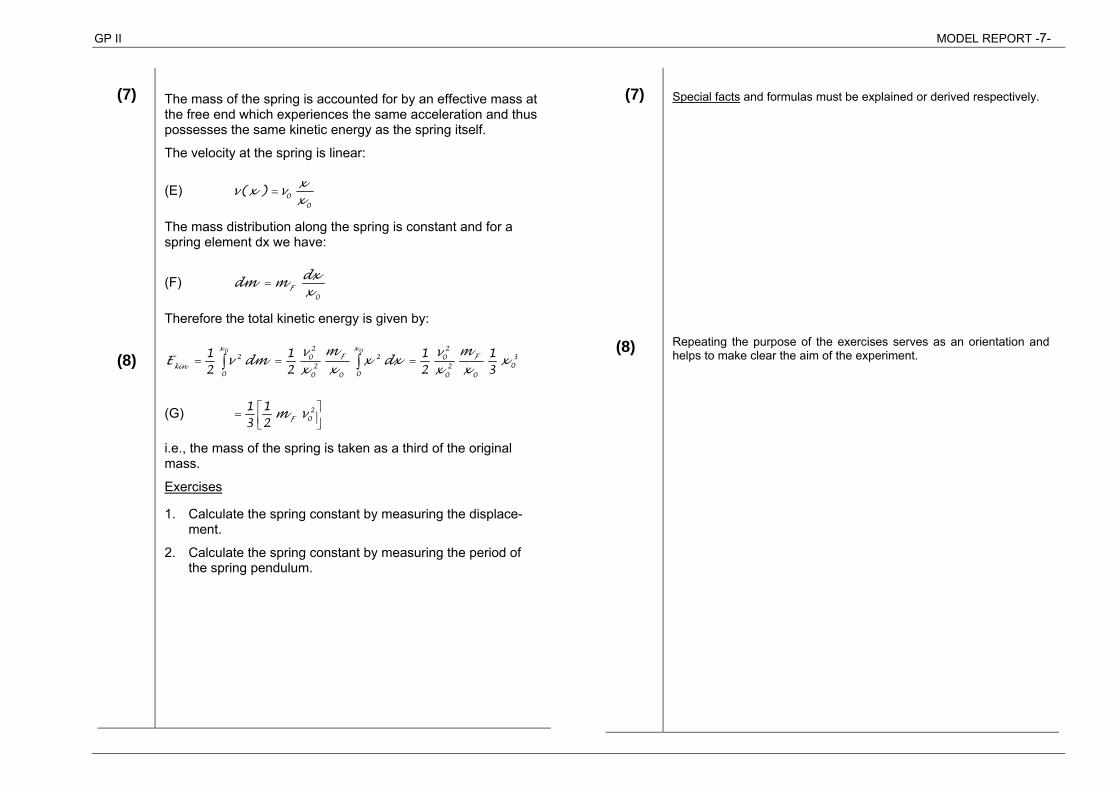
The mass of the spring is accounted for by an effective mass at the free end which experiences the same acceleration and thus possesses the same kinetic energy as the spring itself.

The velocity at the spring is linear:

(E) 0

0)(xxvxv

The mass distribution along the spring is constant and for a spring element dx we have:

(F) 0x

dxmdm F

Therefore the total kinetic energy is given by:

30

02

0

20

0

2

02

0

20

0

2

31

21

21

21 00

xxm

xv

dxxxm

xv

dmvE Fx

Fx

kin

(G)

2

021

31 vm F

i.e., the mass of the spring is taken as a third of the original mass.

Exercises

1. Calculate the spring constant by measuring the displace-ment.

2. Calculate the spring constant by measuring the period of the spring pendulum.

(7)

(8)

Special facts and formulas must be explained or derived respectively.

Repeating the purpose of the exercises serves as an orientation and helps to make clear the aim of the experiment.

GP MODEL REPORT 12-

(9)

(10) (11) (12) (13)

(14)

(15)

(16)

(17)

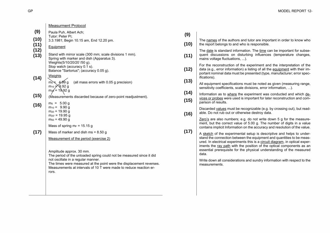
Measurment Protocol Paula Puh, Albert Ach; Tutor: Peter Pi; 3.3.1981; Begin 10.15 am, End 12.20 pm.

Equipment

Stand with mirror scale (300 mm; scale divisions 1 mm). Spring with marker and dish (Apparatus 3). Weights(5/10/20/20´/50 g). Stop watch (accuracy 0.1 s). Balance "Sartorius"; (accuracy 0.05 g). Weights

m5 = 4.99 g (all mass errors with 0.05 g precision) m10 = 9.92 g m20 = 19.92 g

(Measurements discarded because of zero-point readjustment).

m5 = 5.00 g m10 = 9.90 g m20 = 19.90 g m20' = 19.95 g m50 = 49.90 g

Mass of spring mF = 15.15 g

Mass of marker and dish ms = 8.50 g

Measurement of the period (exercise 2)

Amplitude approx. 30 mm. The period of the unloaded spring could not be measured since it did not oscillate in a regular manner. The times were measured at the point were the displacement reverses. Measurements at intervals of 10 T were made to reduce reaction er-rors.

(9)

(10)

(11)

(12)

(13)

(14)

(15)

(16)

(17)

The names of the authors and tutor are important in order to know who the report belongs to and who is responsible.

The date is standard information. The time can be important for subse-quent discussions on disturbing influences (temperature changes, mains voltage fluctuations, ...).

For the reconstruction of the experiment and the interpretation of the data (e.g., error information) a listing of all the equipment with their im-portant nominal data must be presented (type, manufacturer; error spec-ifications).

All equipment specifications must be noted as given (measuring range, sensitivity coefficients, scale divisions, error information, ...).

Information as to where the experiment was conducted and which de-vices or probes were used is important for later reconstruction and com-parison of results.

Discarded values must be recognizable (e.g. by crossing out), but read-able. Do not rub out or otherwise destroy data.

Zero’s are also numbers; e.g. do not write down 5 g for the measure-ment, but the correct value of 5.00 g. The number of digits in a value contains implicit Information on the accuracy and resolution of the value.

A sketch of the experimental setup is descriptive and helps to under-stand the connection between the equipment and quantities to be meas-ured. In electrical experiments this is a circuit diagram, in optical exper-iments the ray path with the position of the optical components as an essential prerequisite for the physical understanding of the measured data.

Write down all considerations and sundry information with respect to the measurements.


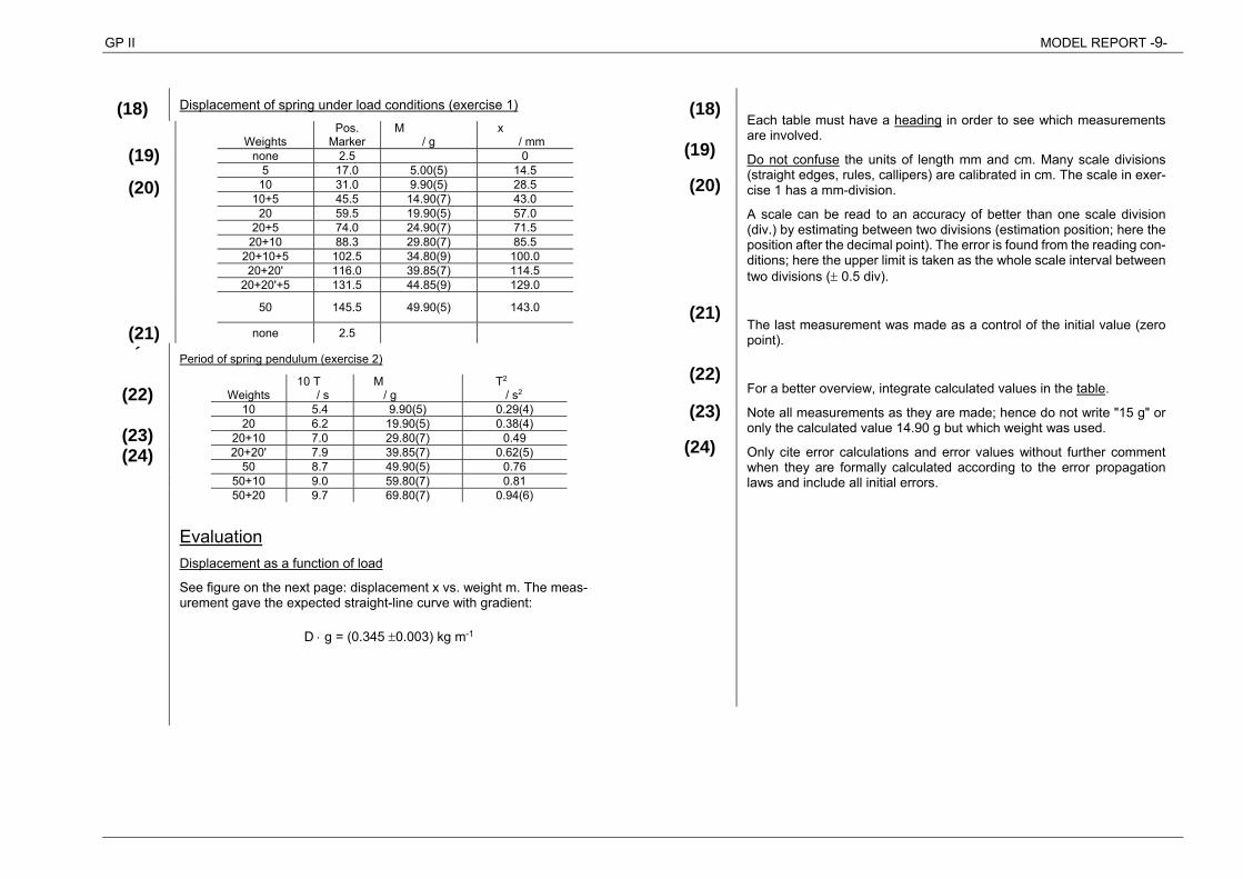
(18) Displacement of spring under load conditions (exercise 1)

(19)

(20)

Pos. M x Weights Marker / g / mm none 2.5 0 5 17.0 5.00(5) 14.5 10 31.0 9.90(5) 28.5 10+5 45.5 14.90(7) 43.0 20 59.5 19.90(5) 57.0 20+5 74.0 24.90(7) 71.5 20+10 88.3 29.80(7) 85.5 20+10+5 102.5 34.80(9) 100.0 20+20' 116.0 39.85(7) 114.5 20+20'+5 131.5 44.85(9) 129.0

50 145.5 49.90(5) 143.0

(21) none 2.5

´

(22)

(23) (24)

Period of spring pendulum (exercise 2)

10 T M T2 Weights / s / g / s2 10 5.4 9.90(5) 0.29(4) 20 6.2 19.90(5) 0.38(4) 20+10 7.0 29.80(7) 0.49 20+20' 7.9 39.85(7) 0.62(5) 50 8.7 49.90(5) 0.76 50+10 9.0 59.80(7) 0.81 50+20 9.7 69.80(7) 0.94(6)

Evaluation Displacement as a function of load

See figure on the next page: displacement x vs. weight m. The meas-urement gave the expected straight-line curve with gradient:

D g = (0.345 0.003) kg m-1

(18)

(19)

(20)

(21)

(22)

(23)

(24)

Each table must have a heading in order to see which measurements are involved.

Do not confuse the units of length mm and cm. Many scale divisions (straight edges, rules, callipers) are calibrated in cm. The scale in exer-cise 1 has a mm-division.

A scale can be read to an accuracy of better than one scale division (div.) by estimating between two divisions (estimation position; here the position after the decimal point). The error is found from the reading con-ditions; here the upper limit is taken as the whole scale interval between two divisions ( 0.5 div).

The last measurement was made as a control of the initial value (zero point).

For a better overview, integrate calculated values in the table.

Note all measurements as they are made; hence do not write "15 g" or only the calculated value 14.90 g but which weight was used.

Only cite error calculations and error values without further comment when they are formally calculated according to the error propagation laws and include all initial errors.

GP MODEL REPORT 12-

(25)

(26)

(27)

(28)

(29)

(30)

(31)

(32)

(33)

(34)

(35)

(36)

(37)

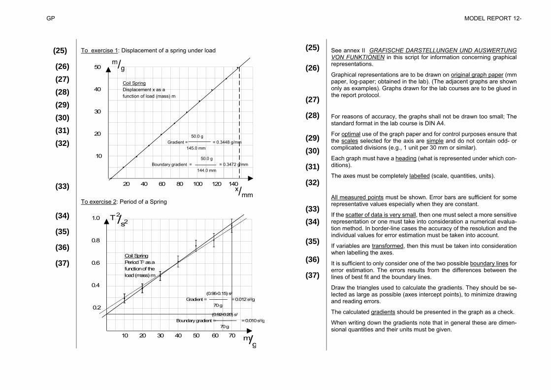
To exercise 1: Displacement of a spring under load

Coil SpringDisplacement x as a function of load (mass) m

20 40 60 80 100 120 140

10

20

30

40

50m/g

x/mm

50.0 g Gradient = = 0.3448 g/mm 145.0 mm

50.0 g Boundary gradient = = 0.3472 g/mm 144.0 mm

To exercise 2: Period of a Spring

10 20 30 40 50 60 70

0.2

0.4

0.6

0.8

1.0

T /s2

m/g

2

(25)

(26)

(27)

(28)

(29)

(30)

(31)

(32)

(33)

(34)

(35)

(36)

(37)

See annex II GRAFISCHE DARSTELLUNGEN UND AUSWERTUNG VON FUNKTIONEN in this script for information concerning graphical representations.

Graphical representations are to be drawn on original graph paper (mm paper, log-paper; obtained in the lab). (The adjacent graphs are shown only as examples). Graphs drawn for the lab courses are to be glued in the report protocol.

For reasons of accuracy, the graphs shall not be drawn too small; The standard format in the lab course is DIN A4.

For optimal use of the graph paper and for control purposes ensure that the scales selected for the axis are simple and do not contain odd- or complicated divisions (e.g., 1 unit per 30 mm or similar).

Each graph must have a heading (what is represented under which con-ditions).

The axes must be completely labelled (scale, quantities, units).

All measured points must be shown. Error bars are sufficient for some representative values especially when they are constant.

If the scatter of data is very small, then one must select a more sensitive representation or one must take into consideration a numerical evalua-tion method. In border-line cases the accuracy of the resolution and the individual values for error estimation must be taken into account.

If variables are transformed, then this must be taken into consideration when labelling the axes.

It is sufficient to only consider one of the two possible boundary lines for error estimation. The errors results from the differences between the lines of best fit and the boundary lines.

Draw the triangles used to calculate the gradients. They should be se-lected as large as possible (axes intercept points), to minimize drawing and reading errors.

The calculated gradients should be presented in the graph as a check.

When writing down the gradients note that in general these are dimen-sional quantities and their units must be given.

Coil SpringPeriod T2 as afunction of theload (mass) m

(0.96-0.15) s2

Gradient = = 0.012 s2/g 70 g

(0.92-0.20) s2

Boundary gradient = = 0.010 s2/g 70 g


(38)

(39)

(40)

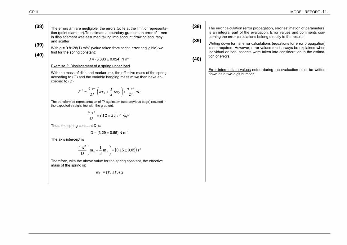
The errors m are negligible, the errors x lie at the limit of representa-tion (point diameter).To estimate a boundary gradient an error of 1 mm in displacement was assumed taking into account drawing accuracy and scatter.

With g = 9.8128(1) m/s2 (value taken from script, error negligible) we find for the spring constant:

D = (3.383 0.024) N m-1

Exercise 2: Displacement of a spring under load

With the mass of dish and marker mS, the effective mass of the spring according to (G) and the variable hanging mass m we then have ac-cording to (D):

mD

mmD

T FS

222 4

314

The transformed representation of T2 against m (see previous page) resulted in the expected straight line with the gradient:

122

)212(4

kgsD

Thus, the spring constant D is:

D = (3.29 0.55) N m-1

The axis intercept is

2FS

2

s05.015.0m31m

D4

Therefore, with the above value for the spring constant, the effective mass of the spring is:

mF = (13 13) g

(38)

(39)

(40)

The error calculation (error propagation, error estimation of parameters) is an integral part of the evaluation. Error values and comments con-cerning the error calculations belong directly to the results.

Writing down formal error calculations (equations for error propagation) is not required. However, error values must always be explained when individual or local aspects were taken into consideration in the estima-tion of errors.

Error intermediate values noted during the evaluation must be written down as a two-digit number.

GP MODEL REPORT 12-

(41)

(42)

(43) (44) (45) (46) (47) (48)

(49)

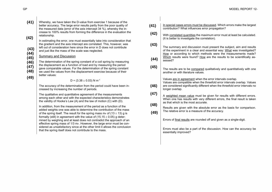
Whereby, we have taken the D-value from exercise 1 because of the better accuracy. The large error results partly from the poor quality of the measured data (error of the axis intercept 34 %), whereby the in-crease to 100% results from forming the difference in the evaluation the relationship.

In estimating the error, one must essentially take into consideration that the gradient and the axis intercept are correlated. This, however, was left out of consideration here since the error in D does not contribute and just like the mass of the scale was neglected.

Summary and Discussion

The determination of the spring constant of a coil spring by measuring the displacement as a function of load and by measuring the period gave comparable values. For the determination of the spring constant we used the values from the displacement exercise because of their better values:

D = (3.38 0.03) N m-1

The accuracy of the determination from the period could have been in-creased by increasing the number of periods.

The qualitative and quantitative agreement of the measurements among each other and with the expected characteristics demonstrates the validity of Hooke’s Law (A) and the law of motion (C) with (D).

In addition, from the measurement of the period as a function of the added weights one was able to determine the contribution of the mass of the spring itself. The result for the spring mass mF of (13 13) g is formally (still) in agreement with the value of (15.15 0.05) g deter-mined by weighing and at least does not contradict the approach of an effective spring mass of 1/3 mF. However, the large error must be con-sidered as unsatisfactory since at the other limit it allows the conclusion that the spring itself does not contribute to the mass.

(41)

(42)

(43)

(44)

(45)

(46)

(47)

(48)

(49)

In special cases errors must be discussed. Which errors make the largest contribution? What influences error propagation? With correlated quantities the maximum error must at least be calculated. (It is better to investigate the correlation).

The summary and discussion must present the subject, aim and results of the experiment in a clear and essential way: What was investigated? How or according to which methods were the measurements made? Which results were found? How are the results to be scientifically as-sessed?

The results are to be compared qualitatively and quantitatively with one another or with literature values. Values are in agreement when the error intervals overlap. Values are compatible when the threefold error intervals overlap. Values are considered significantly different when the threefold error intervals no longer overlap. A weighted mean value must be given for results with different errors. When one has results with very different errors, the final result is taken as that which is the most accurate.

Results are given with the absolute error as the basis for comparison. The relative error is a measure of the accuracy.

Errors of final results are rounded off and given as a single-digit.

Errors must also be a part of the discussion. How can the accuracy be essentially improved?

GP II STANDARD TEXT BOOKS-13-

STANDARDLEHRBÜCHER GP

Die folgenden Lehrbücher werden verbreitet zur Vermitt-lung physikalischen Grundwissens herangezogen, wie es für das Physikstudium und die Vorbereitung der Prak-tikumsarbeit erforderlich ist. Eine Reihe von Lehrbüchern wurden in verschiedenen Auflagen bzw. Jahren heraus-gegeben, so daß auf eine Angabe des Erscheinungs-jahrs verzichtet wurde. Alle Bücher sind in der Lehrbuch-sammlung der Fachbereichsbibliothek vorhanden.

obligatorische Literatur

[1]: GerthsenKneserVogel; Physik; Springer-Verlag

[2]: Bergmann-Schaefer Band 1 (11. Auflage)



[5]: Eichler Kronfeld Sahm

Das neue Physiklaische Praktikum

Zusatzliteratur

AlonsoFinn; Physik; Addison-Wesley bzw. Inter European Editions

Atkins; Physik; de Gruyter

KittelKnightRudermann; Berkeley Physik Kurs (1: Mechanik, 2: Elektrizität und Magnetismus, 3: Schwingungen und Wellen, 4: Quantenphysik, 5: Statistische Physik); Vieweg & Sohn

Demtröder; Experimentalphysik 1-4; Springer-Verlag

DransfeldKalviusKienleLucherVonach; Physik (I: Mechanik, II: Elektrodynamik, IV: Atome-Moleküle-Wärme); Oldenbourg

FeynmanLeightonSands; Vorlesungen über Physik (I: Mechanik-Strahlung-Wärme, II: Elektromagnetismus und Struktur der Materie); Oldenbourg

HänselNeumann; Physik 1-3; Spektrum Akademische Verlagsanstalt

Kohlrausch; Praktische Physik (3: Tafeln); Teubner

Tipler; Physik; Spektrum Akademische Verlagsanstalt

Martienssen; Einführung in die Physik (I: Mechanik, II: Elektrodynamik, III: Thermodynamik, IV: Schwingungen-Wellen-Quanten); Akademische Verlagsgesellschaft

Otten; Repititorium der Experimentalphysik; Springer-Verlag

PSSC; Vieweg

Pohl, Einführung in die Physik (1: Mechanik-Akustik-Wärme, 2: Elektrizitätslehre, 3: Optik-Atomphysik); Springer-Verlag

ZinthKörner; Physik I-III; Oldenbourg

Westphal; Kleines Lehrbuch der Physik; Springer-Verlag

Optik

BornWolf; Principles of Optics; Mac Millan

Fowles; Introduction to Modern Optics; Dover Publication Inc.

Atom- und Quantenphysik

EisbergResnick; Quatum Physics of Atoms, Moleculs, Solids, Nuclei and Particles; Wiley & Sons

Finkelnburg; Atomphysik; Springer-Verlag

HakenWolf; Atom- und Quantenphysik; Springer-Verlag

Beiser; Atome, Moleküle, Festkörper; Vieweg & Sohn

Fehlerrechnung

Taylor; Fehleranalyse; VCH Verlagsgesellschaft

GP MICROSCOPE 14-

14

MICROSCOPE GP II

Key Words

Geometrical Optics; Imaging with Lenses. Resolution and diffraction limit; Abbe’s Theory, numeri-cal aperture.

Aim of the Experiment

Understanding the working principles of a microscope and handling optical components and instruments.

Literature

Standard literature (see list of standard text books).

Exercises

1. Determining the focal length of a lens using the Bessel Method.

2. Constructing the ray path of a microscope. Deter-mining the magnification for three different tube lengths and comparing the results with the theo-retical expectations.

3. Calibrating an ocular micrometer (measurement ocular). Determining the grating constant and the thickness of the wires of a wire grating (cross grat-ing).

4. Verification of Abbe’s Theory. Observing the reso-lution limit of the microscope using the wire grat-ing. Determining the numerical aperture for this limiting case and comparing the expected smallest resolvable point separation with the measured grating constant.

5. Calculation exercise: Specifying the smallest re-solvable point separation for the strongest objec-tive (numerical aperture 1.4 with immersion fluid) and hence the achievable meaningful limit of mag-nification of a microscope.

Physical Principles

Imaging through Lenses

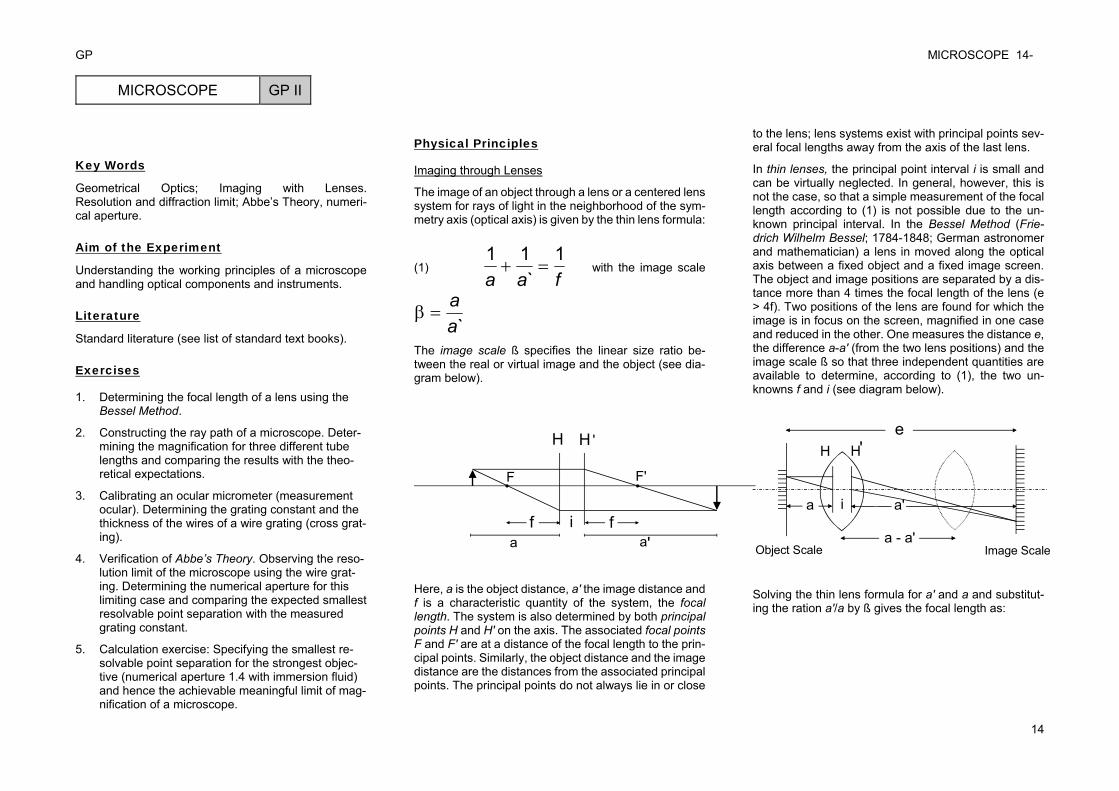
The image of an object through a lens or a centered lens system for rays of light in the neighborhood of the sym-metry axis (optical axis) is given by the thin lens formula:

(1) faa1

`11 with the image scale

àa

The image scale ß specifies the linear size ratio be-tween the real or virtual image and the object (see dia-gram below).

F F'

H H '

if fa a'

Here, a is the object distance, a' the image distance and f is a characteristic quantity of the system, the focal length. The system is also determined by both principal points H and H' on the axis. The associated focal points F and F' are at a distance of the focal length to the prin-cipal points. Similarly, the object distance and the image distance are the distances from the associated principal points. The principal points do not always lie in or close

to the lens; lens systems exist with principal points sev-eral focal lengths away from the axis of the last lens.

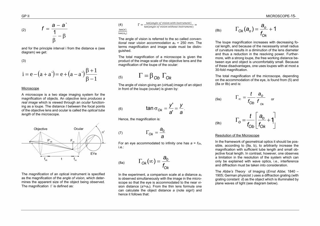
In thin lenses, the principal point interval i is small and can be virtually neglected. In general, however, this is not the case, so that a simple measurement of the focal length according to (1) is not possible due to the un-known principal interval. In the Bessel Method (Frie-drich Wilhelm Bessel; 1784-1848; German astronomer and mathematician) a lens in moved along the optical axis between a fixed object and a fixed image screen. The object and image positions are separated by a dis-tance more than 4 times the focal length of the lens (e > 4f). Two positions of the lens are found for which the image is in focus on the screen, magnified in one case and reduced in the other. One measures the distance e, the difference a-a' (from the two lens positions) and the image scale ß so that three independent quantities are available to determine, according to (1), the two un-knowns f and i (see diagram below).

a - a'

a a'i

eH H'

Object Scale Image Scale

Solving the thin lens formula for a' and a and substitut-ing the ration a'/a by ß gives the focal length as:

GP II MICROSCOPE-15-

(2)

1àaf

and for the principle interval i from the distance e (see diagram) we get:

(3)

11àaeàaei

Microscope

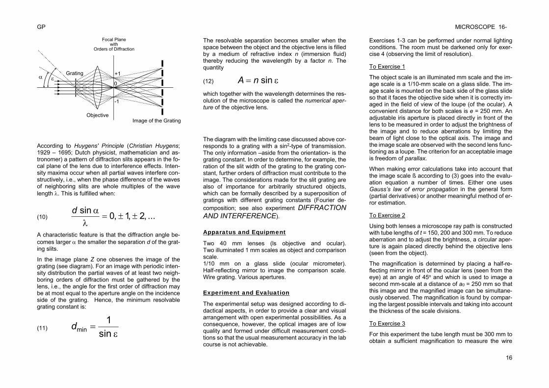
A microscope is a two stage imaging system for the magnification of objects. An objective lens produces a real image which is viewed through an ocular function-ing as a loupe. The distance t between the focal points of the objective lens and ocular is called the optical tube length of the microscope.

'

EYe

OcularObjective

F'ob Foc

fob t foc

The magnification of an optical instrument is specified as the magnification of the angle of vision, which deter-mines the apparent size of the object being observed. The magnification is defined as:

(4) Γ

The angle of vision is referred to the so called conven-tional near vision accommodation ao = 250 mm. The terms magnification and image scale must be distin-guished.

The total magnification of a microscope is given the product of the image scale of the objective lens and the magnification of the loupe of the ocular:

(5) OkOb

The angle of vision giving an (virtual) image of an object in front of the loupe (ocular) is given by:

(6) ay

ay

Ok ''tan .

Hence, the magnification is:

(7) aa

Ok0

For an eye accommodated to infinity one has a = fOk, i.e.:

(8a) Ok

Ok fa0)(

In the experiment, a comparison scale at a distance ao is observed simultaneously with the image in the micro-scope so that the eye is accommodated to the near vi-sion distance (a'=ao). From the thin lens formula one can calculate the object distance a (note sign!) and hence it follows that:

(8b) 1)( Ok

ooOk f

aa

The loupe magnification increases with decreasing fo-cal length, and because of the necessarily small radius of curvature results in a diminution of the lens diameter and thus a reduction in the resolving power. Further-more, with a strong loupe, the free working distance be-tween eye and object is uncomfortably small. Because of these disadvantages, one uses loupes with at most a 30-fold magnification.

The total magnification of the microscope, depending on the accommodation of the eye, is found from (5) and (8a or 8b) and is:

(9a) Ok

fa

ft o

Ob or

(9b)

1

Ok

o

Obo f

aft

Resolution of the Microscope

In the framework of geometrical optics it should be pos-sible, according to (9a, b), to arbitrarily increase the magnification with sufficient tube length and small ob-jective focal length. In contrast, however, one observes a limitation in the resolution of the system which can only be explained with wave optics, i.e., interference and diffraction must be taken into consideration.

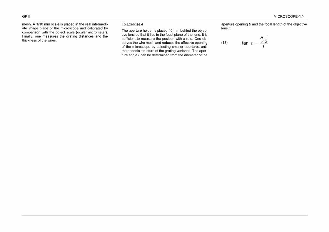
The Abbe’s Theory of Imaging (Ernst Abbe; 1840 – 1905; German physicist ) uses a diffraction grating (with grating constant d) as the object which is illuminated by plane waves of light (see diagram below).

GP MICROSCOPE 16-

16

Grating

Objective

Focal Planewith

Orders of Diffraction

Image of the Grating

+1

-1

0

According to Huygens' Principle (Christian Huygens; 1929 – 1695; Dutch physicist, mathematician and as-tronomer) a pattern of diffraction slits appears in the fo-cal plane of the lens due to interference effects. Inten-sity maxima occur when all partial waves interfere con-structively, i.e., when the phase difference of the waves of neighboring slits are whole multiples of the wave length . This is fulfilled when:

(10) ...,2,1,0sin

d

A characteristic feature is that the diffraction angle be-comes larger the smaller the separation d of the grat-ing slits.

In the image plane Z one observes the image of the grating (see diagram). For an image with periodic inten-sity distribution the partial waves of at least two neigh-boring orders of diffraction must be gathered by the lens, i.e., the angle for the first order of diffraction may be at most equal to the aperture angle on the incidence side of the grating. Hence, the minimum resolvable grating constant is:

(11)

sin

1mind

The resolvable separation becomes smaller when the space between the object and the objective lens is filled by a medium of refractive index n (immersion fluid) thereby reducing the wavelength by a factor n. The quantity

(12) sinnA

which together with the wavelength determines the res-olution of the microscope is called the numerical aper-ture of the objective lens.

The diagram with the limiting case discussed above cor-responds to a grating with a sin2-type of transmission. The only information –aside from the orientation- is the grating constant. In order to determine, for example, the ration of the slit width of the grating to the grating con-stant, further orders of diffraction must contribute to the image. The considerations made for the slit grating are also of importance for arbitrarily structured objects, which can be formally described by a superposition of gratings with different grating constants (Fourier de-composition; see also experiment DIFFRACTION AND INTERFERENCE).

Apparatus and Equipment

Two 40 mm lenses (ls objective and ocular). Two illuminated 1 mm scales as object and comparison scale. 1/10 mm on a glass slide (ocular micrometer). Half-reflecting mirror to image the comparison scale. Wire grating. Various apertures.

Experiment and Evaluation

The experimental setup was designed according to di-dactical aspects, in order to provide a clear and visual arrangement with open experimental possibilities. As a consequence, however, the optical images are of low quality and formed under difficult measurement condi-tions so that the usual measurement accuracy in the lab course is not achievable.

Exercises 1-3 can be performed under normal lighting conditions. The room must be darkened only for exer-cise 4 (observing the limit of resolution).

To Exercise 1

The object scale is an illuminated mm scale and the im-age scale is a 1/10-mm scale on a glass slide. The im-age scale is mounted on the back side of the glass slide so that it faces the objective side when it is correctly im-aged in the field of view of the loupe (of the ocular). A convenient distance for both scales is e = 250 mm. An adjustable iris aperture is placed directly in front of the lens to be measured in order to adjust the brightness of the image and to reduce aberrations by limiting the beam of light close to the optical axis. The image and the image scale are observed with the second lens func-tioning as a loupe. The criterion for an acceptable image is freedom of parallax.

When making error calculations take into account that the image scale ß according to (3) goes into the evalu-ation equation a number of times. Either one uses Gauss’s law of error propagation in the general form (partial derivatives) or another meaningful method of er-ror estimation.

To Exercise 2

Using both lenses a microscope ray path is constructed with tube lengths of t = 150, 200 and 300 mm. To reduce aberration and to adjust the brightness, a circular aper-ture is again placed directly behind the objective lens (seen from the object).

The magnification is determined by placing a half-re-flecting mirror in front of the ocular lens (seen from the eye) at an angle of 45o and which is used to image a second mm-scale at a distance of a0 = 250 mm so that this image and the magnified image can be simultane-ously observed. The magnification is found by compar-ing the largest possible intervals and taking into account the thickness of the scale divisions.

To Exercise 3

For this experiment the tube length must be 300 mm to obtain a sufficient magnification to measure the wire

GP II MICROSCOPE-17-

mesh. A 1/10 mm scale is placed in the real intermedi-ate image plane of the microscope and calibrated by comparison with the object scale (ocular micrometer). Finally, one measures the grating distances and the thickness of the wires.

To Exercise 4

The aperture holder is placed 40 mm behind the objec-tive lens so that it lies in the focal plane of the lens. It is sufficient to measure the position with a rule. One ob-serves the wire mesh and reduces the effective opening of the microscope by selecting smaller apertures until the periodic structure of the grating vanishes. The aper-ture angle can be determined from the diameter of the

aperture opening B and the focal length of the objective lens f:

(13) f

B2tan

GP OPTICAL SEPCTROSCOPY 22-

18

OPTICAL SPECTROSCOPY GP II

Key Words

Dispersion; Prisms. Diffraction and Interference; Dif-fraction Grating. Spectral Equipment and Spectral Analysis.


Phenomenological and experimental introduction into the fundamentals of optical spectroscopy as an im-portant scientific and applied analytical tool in many ar-eas of the natural sciences.

Literature


Exercises

Performing experiments either with the prism spectrom-eter or grating spectrometer:

Prism Spectrometer

1. Setting up and adjusting the spectrometer (illumi-nation, collimator, telescope).

2. Measuring the angle of the refracting edge of a prism.

3. Recording the spectrum of a mercury lamp to cali-brate the spectrometer.

4. Performing one of the following experiments.

5. Plotting the dispersion curve n() and determining the differential dispersion dn/d for the 577/579 nm line of mercury.

6. Determining the resolving power of the prism and comparing the result with the theoretical expecta-tion.

7. Qualitative observation and discussion of the dif-fraction spectrum of a grating.

Grating Spectrometer

2. Recording the spectrum of a mercury lamp in the first and second order and determining the grating constant.

3. Performing one of the following experiments.

4. Determining the resolving power of the grating in the first and second order and comparing the re-sult with the theoretical expectations.

5. Qualitative observation and discussion of the dis-persion spectrum of a prism.

Spectroscopic Tasks

Spectroscopic analysis of an unknown lamp and deter-mining its gas content.

Physical Principles

Prism

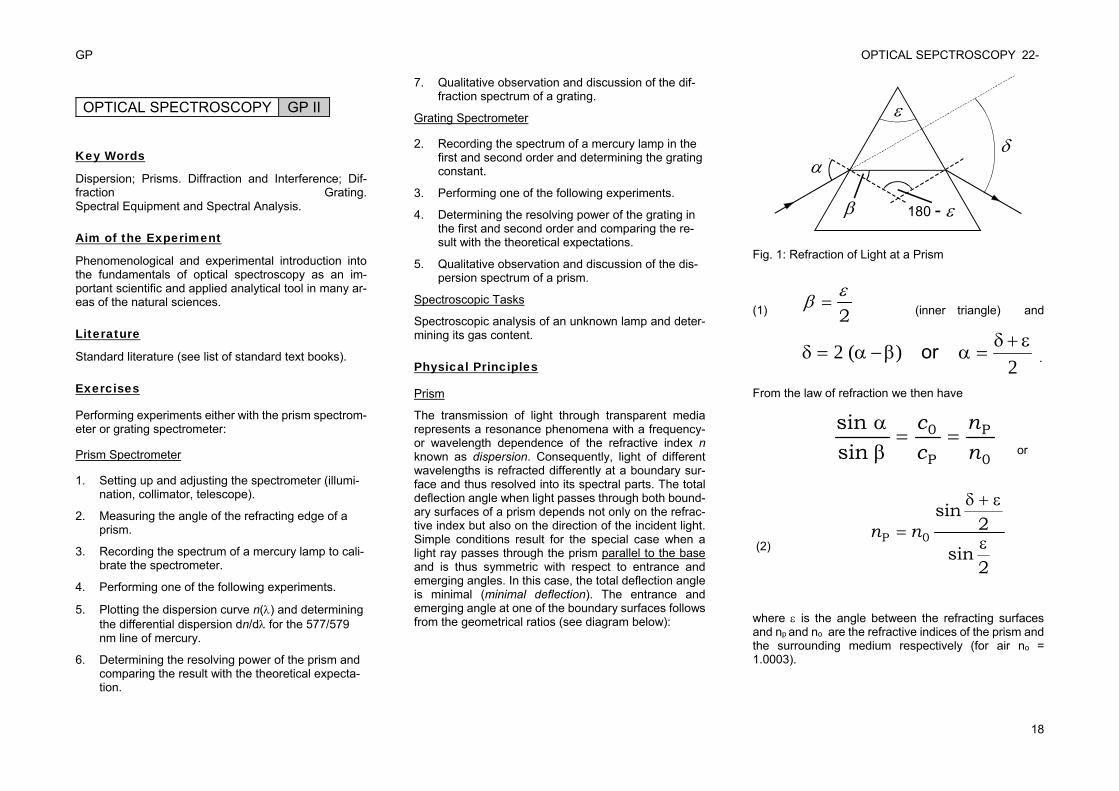
The transmission of light through transparent media represents a resonance phenomena with a frequency- or wavelength dependence of the refractive index n known as dispersion. Consequently, light of different wavelengths is refracted differently at a boundary sur-face and thus resolved into its spectral parts. The total deflection angle when light passes through both bound-ary surfaces of a prism depends not only on the refrac-tive index but also on the direction of the incident light. Simple conditions result for the special case when a light ray passes through the prism parallel to the base and is thus symmetric with respect to entrance and emerging angles. In this case, the total deflection angle is minimal (minimal deflection). The entrance and emerging angle at one of the boundary surfaces follows from the geometrical ratios (see diagram below):

180 -

Fig. 1: Refraction of Light at a Prism

(1) 2 (inner triangle) and

2)(2

or .

From the law of refraction we then have

0

P

P

0

sinsin

nn

cc

or

(2)

2sin

2sin

0P

nn

where is the angle between the refracting surfaces and np and no are the refractive indices of the prism and the surrounding medium respectively (for air no = 1.0003).

GP II OPTICAL SPECTROSCOPY19-

Prisms find application is spectroscopy and light filter-ing. The dispersion power and the refractive index are independent of one another. For example, the refractive index of flint glass is only slightly higher than that of crown glass, however, the dispersion power is almost twice as high. The different behavior of various types of glass allows the construction of prisms with strong de-flection properties but do not disperse (deflection prism, achromatic prism) or prism with strong dispersion prop-erties but do not deflect (direct vision prism).

Resolution Criterion

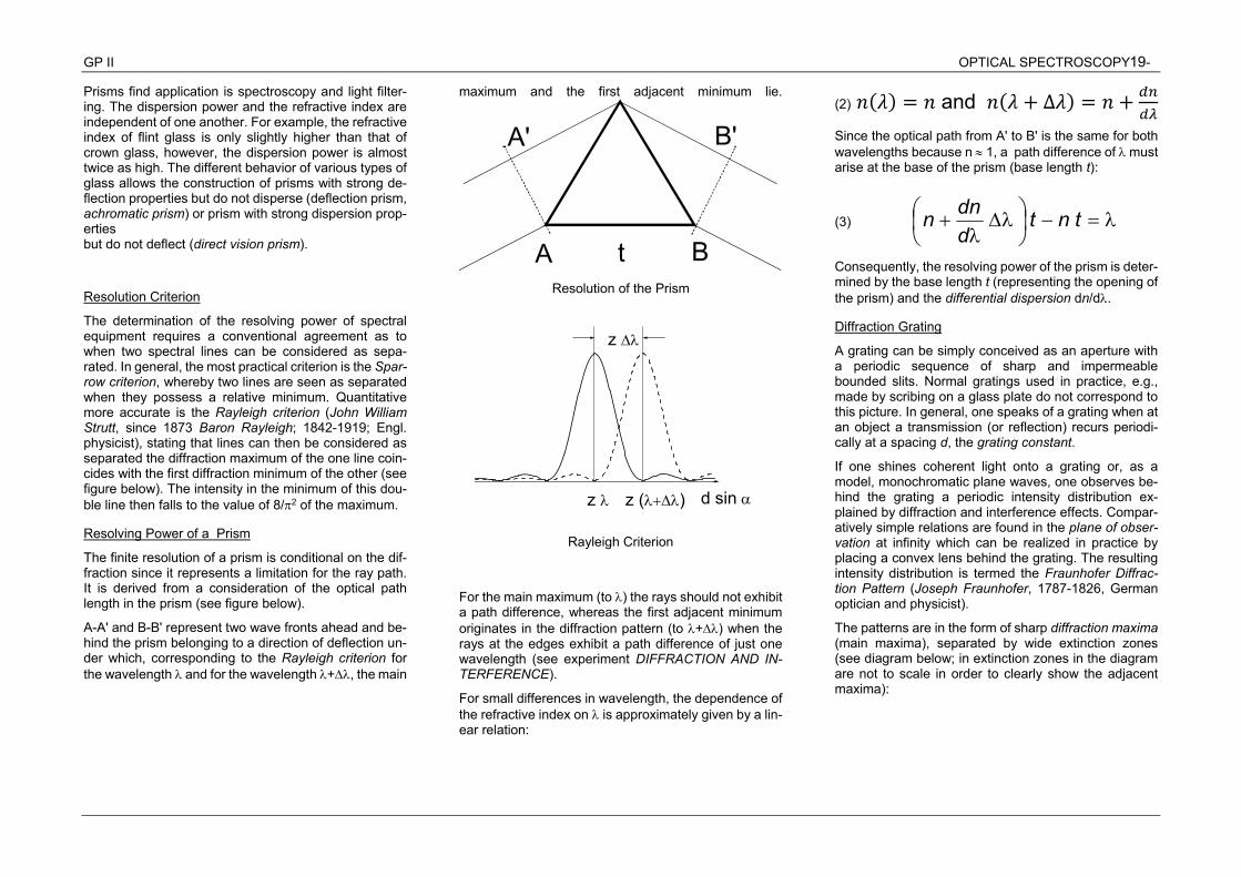
The determination of the resolving power of spectral equipment requires a conventional agreement as to when two spectral lines can be considered as sepa-rated. In general, the most practical criterion is the Spar-row criterion, whereby two lines are seen as separated when they possess a relative minimum. Quantitative more accurate is the Rayleigh criterion (John William Strutt, since 1873 Baron Rayleigh; 1842-1919; Engl. physicist), stating that lines can then be considered as separated the diffraction maximum of the one line coin-cides with the first diffraction minimum of the other (see figure below). The intensity in the minimum of this dou-ble line then falls to the value of 8/2 of the maximum.

Resolving Power of a Prism

The finite resolution of a prism is conditional on the dif-fraction since it represents a limitation for the ray path. It is derived from a consideration of the optical path length in the prism (see figure below).

A-A' and B-B' represent two wave fronts ahead and be-hind the prism belonging to a direction of deflection un-der which, corresponding to the Rayleigh criterion for the wavelength and for the wavelength +, the main

maximum and the first adjacent minimum lie.

A

A' B'

Bt

Resolution of the Prism

Rayleigh Criterion

For the main maximum (to ) the rays should not exhibit a path difference, whereas the first adjacent minimum originates in the diffraction pattern (to +) when the rays at the edges exhibit a path difference of just one wavelength (see experiment DIFFRACTION AND IN-TERFERENCE).

For small differences in wavelength, the dependence of the refractive index on is approximately given by a lin-ear relation:

(2) and Δ

Since the optical path from A' to B' is the same for both wavelengths because n 1, a path difference of must arise at the base of the prism (base length t):

(3)

tnt

ddnn

Consequently, the resolving power of the prism is deter-mined by the base length t (representing the opening of the prism) and the differential dispersion dn/d.

Diffraction Grating

A grating can be simply conceived as an aperture with a periodic sequence of sharp and impermeable bounded slits. Normal gratings used in practice, e.g., made by scribing on a glass plate do not correspond to this picture. In general, one speaks of a grating when at an object a transmission (or reflection) recurs periodi-cally at a spacing d, the grating constant.

If one shines coherent light onto a grating or, as a model, monochromatic plane waves, one observes be-hind the grating a periodic intensity distribution ex-plained by diffraction and interference effects. Compar-atively simple relations are found in the plane of obser-vation at infinity which can be realized in practice by placing a convex lens behind the grating. The resulting intensity distribution is termed the Fraunhofer Diffrac-tion Pattern (Joseph Fraunhofer, 1787-1826, German optician and physicist).

The patterns are in the form of sharp diffraction maxima (main maxima), separated by wide extinction zones (see diagram below; in extinction zones in the diagram are not to scale in order to clearly show the adjacent maxima):

d sin z ()z

z


20

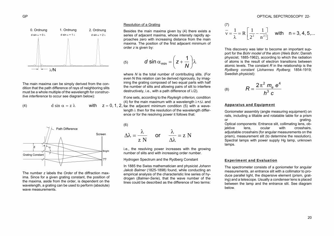
The main maxima can be simply derived from the con-dition that the path difference of rays of neighboring slits must be a whole multiple of the wavelength for construc-tive interference to occur see diagram below):

(4) ....2,1,0,z with zsind

Screen

Bright

??

Path Difference

d

Grating Constant

The number z labels the Order of the diffraction max-ima. Since for a given grating constant, the position of the maxima, aside from the order, is dependent on the wavelength, a grating can be used to perform (absolute) wave measurements.

Resolution of a Grating

Besides the main maxima given by (4) there exists a series of adjacent maxima, whose intensity rapidly ap-proaches zero with increasing distance from the main maxima. The position of the first adjacent minimum of order z is given by:

(5)

Nzd 1sin min

where N is the total number of contributing slits. (For even N this relation can be derived rigorously, by imag-ining the grating composed of two equal parts with half the number of slits and allowing pairs of slit to interfere destructively, i.e., with a path difference of /2).

If one sets, according to the Rayleigh criterion, condition (4) for the main maximum with a wavelength + and for the adjacent minimum condition (5) with a wave-length then for the resolution of the wavelength differ-ence or for the resolving power it follows that:

(6)

NzNz

or

i.e., the resolving power increases with the growing number of slits and with increasing order number.

Hydrogen Spectrum and the Rydberg Constant

In 1885 the Swiss mathematician and physicist Johann Jakob Balmer (1825-1898) found, while conducting an empirical analysis of the characteristic line series of hy-drogen (Balmer-Serie), that the wave number of the lines could be described as the difference of two terms:

(7)

5,...4,3,n with

22 n

121R1

This discovery was later to become an important sup-port for the Bohr model of the atom (Niels Bohr; Danish physicist; 1885-1962), according to which the radiation of atoms is the result of electron transitions between atomic levels. The constant R in the relationship is the Rydberg constant (Johannes Rydberg; 1854-1919; Swedish.physicist):

(8) ch

emR e3

422


Goniometer assembly (angle measuring equipment) on rails, including a tiltable and rotatable table for a prism or grating. Optical components: Entrance slit, collimating lens, ob-jektive lens, ocular with crosshairs. adjustable crosshairs (for angular measurements on the prism), measurement slit (to determine the resolution). Spectral lamps with power supply Hg lamp, unknown lamps.


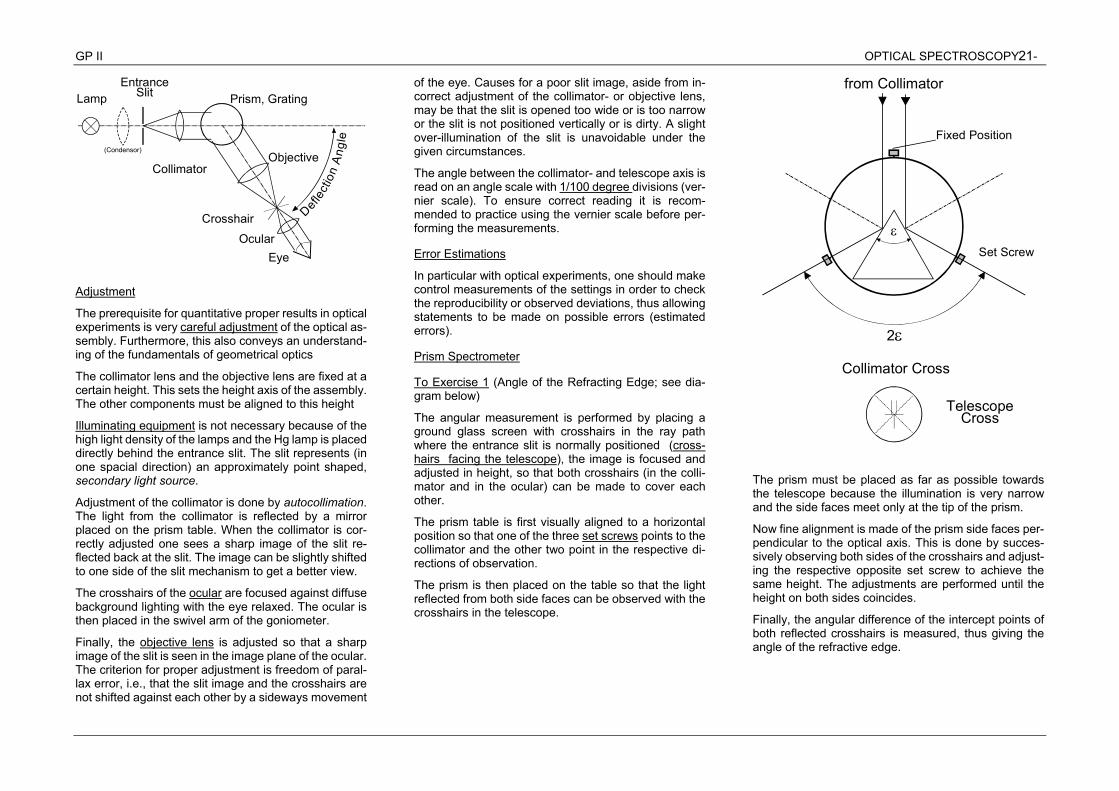
The spectrometer consists of a goniometer for angular measurements, an entrance slit with a collimator to pro-duce parallel light, the dispersive element (prism, grat-ing) and a telescope. Usually a condenser lens is placed between the lamp and the entrance slit. See diagram below.

d sin = 2 d sin = 1 d sin = 0

/N

2. Ordnung1. Ordnung0. Ordnung


Lamp

(Condensor)

EntranceSlit

Collimator

Prism, Grating

Objective

Crosshair

OcularEye

Defle

ctio

n A

ngle

Adjustment

The prerequisite for quantitative proper results in optical experiments is very careful adjustment of the optical as-sembly. Furthermore, this also conveys an understand-ing of the fundamentals of geometrical optics

The collimator lens and the objective lens are fixed at a certain height. This sets the height axis of the assembly. The other components must be aligned to this height

Illuminating equipment is not necessary because of the high light density of the lamps and the Hg lamp is placed directly behind the entrance slit. The slit represents (in one spacial direction) an approximately point shaped, secondary light source.

Adjustment of the collimator is done by autocollimation. The light from the collimator is reflected by a mirror placed on the prism table. When the collimator is cor-rectly adjusted one sees a sharp image of the slit re-flected back at the slit. The image can be slightly shifted to one side of the slit mechanism to get a better view.

The crosshairs of the ocular are focused against diffuse background lighting with the eye relaxed. The ocular is then placed in the swivel arm of the goniometer.

Finally, the objective lens is adjusted so that a sharp image of the slit is seen in the image plane of the ocular. The criterion for proper adjustment is freedom of paral-lax error, i.e., that the slit image and the crosshairs are not shifted against each other by a sideways movement

of the eye. Causes for a poor slit image, aside from in-correct adjustment of the collimator- or objective lens, may be that the slit is opened too wide or is too narrow or the slit is not positioned vertically or is dirty. A slight over-illumination of the slit is unavoidable under the given circumstances.

The angle between the collimator- and telescope axis is read on an angle scale with 1/100 degree divisions (ver-nier scale). To ensure correct reading it is recom-mended to practice using the vernier scale before per-forming the measurements.

Error Estimations

In particular with optical experiments, one should make control measurements of the settings in order to check the reproducibility or observed deviations, thus allowing statements to be made on possible errors (estimated errors).

Prism Spectrometer

To Exercise 1 (Angle of the Refracting Edge; see dia-gram below)

The angular measurement is performed by placing a ground glass screen with crosshairs in the ray path where the entrance slit is normally positioned (cross-hairs facing the telescope), the image is focused and adjusted in height, so that both crosshairs (in the colli-mator and in the ocular) can be made to cover each other.

The prism table is first visually aligned to a horizontal position so that one of the three set screws points to the collimator and the other two point in the respective di-rections of observation.

The prism is then placed on the table so that the light reflected from both side faces can be observed with the crosshairs in the telescope.

2

from Collimator

Fixed Position

Set Screw

Collimator Cross

TelescopeCross

The prism must be placed as far as possible towards the telescope because the illumination is very narrow and the side faces meet only at the tip of the prism.

Now fine alignment is made of the prism side faces per-pendicular to the optical axis. This is done by succes-sively observing both sides of the crosshairs and adjust-ing the respective opposite set screw to achieve the same height. The adjustments are performed until the height on both sides coincides.

Finally, the angular difference of the intercept points of both reflected crosshairs is measured, thus giving the angle of the refractive edge.


22

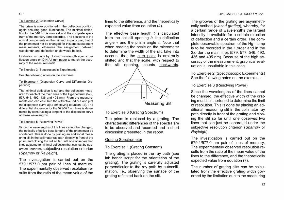
To Exercise 2 (Calibration Curve)

The prism is now positioned in the deflection position, again ensuring good illumination. The minimal deflec-tion for the 546 nm is now set and the complete spec-trum of the mercury lamp recorded. The positions of the optical components on the rail and, in particular, that of the prism must not be changed for this and subsequent measurements, otherwise the assignment between wavelength and deflection angle would be lost.

Evaluation is made by plotting wavelength against de-flection angle on DIN-A4 mm paper to match the accu-racy of the measurements!

To Exercise 3 (Spectroscopic Experiments)

See the following notes on the exercises.

To Exercise 4 (Dispersion Curve and Differential Dis-persion)

The minimal deflection is set and the deflection meas-ured for each of the main lines of the Hg-spectrum (579, 577, 546, 492, 436 and 405 nm). From the measure-ments one can calculate the refractive indices and plot the dispersion curve n() employing equation (2). The differential dispersion for the 579/577 nm lines is deter-mined by constructing a tangent to the dispersion curve at these wavelengths.

To Exercise 5 (Resolving Power)

Since the wavelengths of the lines cannot be changed, the optically effective base length t of the prism must be shortened. This is done by placing an additional meas-uring slit in the collimator ray path directly in front of the prism and closing the slit so far until one observes two lines adjusted to minimal deflection that can just be sep-arated under the subjective resolution criterion (Sparrow or Rayleigh).

The investigation is carried out on the 579.1/577.0 nm pair of lines of mercury. The experimentally observed resolution re-sults from the ratio of the mean value of the

lines to the difference, and the theoretically expected value from equation (4).

The effective base length t is calculated from the set slit opening b, the deflection angle and the prism angle . Note that when reading the scale on the micrometer to determine the width of the slit, take into account that the zero point is arbitrarily shifted and that the scale, with respect to the slit opening, counts backwards.

tMeasuring Slit

To Exercise 6 (Grating Spectrum)

The prism is replaced by a grating. The characteristic differences of the spectra are to be observed and recorded and a short discussion presented in the report.

Grating Spectrometer

To Exercise 1 (Grating Constant)

The grating is placed in the ray path (see lab bench script for the orientation of the grating). The grating is carefully adjusted perpendicular to the ray path by autocolli-mation, i.e., observing the surface of the grating reflected back on the slit.

The grooves of the grating are asymmetri-cally scribed (blazed grating), whereby, for a certain range of wavelengths the largest intensity is available for a certain direction of deflection and a certain order. The com-plete observable spectrum of the Hg - lamp is to be recorded in the 1.order and in the 2.order the main lines (579, 577, 546, 492, 436 and 405 nm). Because of the high ac-curacy of the measurement, graphical eval-uation is unsuitable in this case.

To Exercise 2 (Spectroscopic Experiments) See the following notes on the exercises.

To Exercise 3 (Resolving Power)

Since the wavelengths of the lines cannot be changed, the effective width of the grat-ing must be shortened to determine the limit of resolution. This is done by placing an ad-ditional measuring slit in the collimator ray path directly in front of the grating and clos-ing the slit so far until one observes two lines that can just be separated under the subjective resolution criterion (Sparrow or Rayleigh).

The investigation is carried out on the 579.1/577.0 nm pair of lines of mercury. The experimentally observed resolution re-sults from the ratio of the mean value of the lines to the difference, and the theoretically expected value from equation (7).

The number of grating slits can be calcu-lated from the effective grating width gov-erned by the limitation due to the measuring


slit and from the grating constant. Note that when reading the scale on the micrometer to determine the width of the slit, take into account that the zero point is arbitrarily shifted and that the scale, with respect to the slit opening, counts backwards.

To Exercise 5 (Prism Spectrum)

The grating is replaced by a prism. The characteristic differences of the spectra are

to be observed and recorded and a short discussion presented in the report.

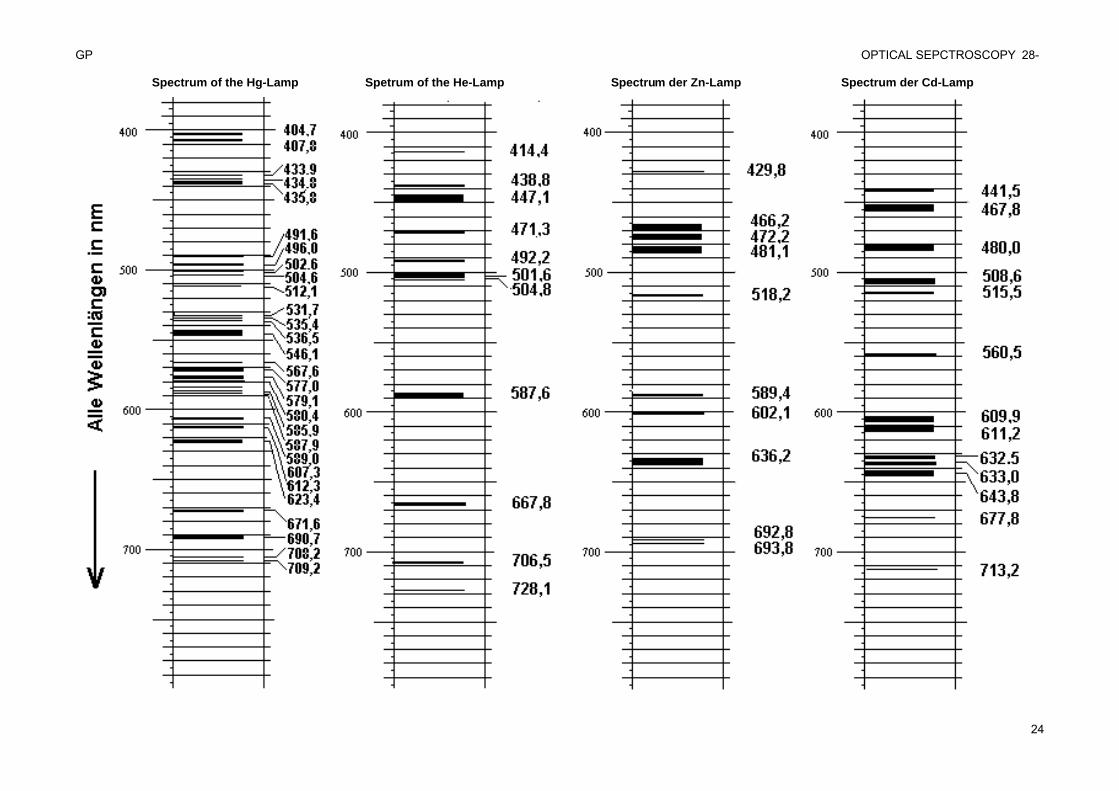
Spectroscopic Experiments Unknown Lamps The spectrum of one (of the three available) unknown lamps is recoded and the ob-served wavelengths determined from the calibration curve or the grating constant. The results are analysed using the table of selected spectral line attached to this script.

Spectral Lines See the following page for the spectrum of the Hg-lamp and the lines of Cd, He and Zn.


24

Spectrum of the Hg-Lamp Spetrum of the He-Lamp Spectrum der Zn-Lamp Spectrum der Cd-Lamp

GP II DIFFRACTION AND INTERFERENCE 25-

DIFFRACTION AND INTERFERENCE GP II

Key Words

Wave optics; Huygens Principle. Coherence. Diffraction and interference at slits and gratings.


Experimental introduction to diffraction phenomena. Wave treatment of optical images (Abbe’s Theory) and the interconnection between diffraction patterns and the image of an object. Exemplary investigation of image filtering.

Literature


Exercises

One can select between exercises employing a thermal spectral lamp (exercise A) or a He-Ne laser (exercise B).

Exercises using a Na-spectral lamp (exercise A)

A1. Constructing the ray path and determining the im-age scale of the microscopic image. A2. Determining the width of a single slit from the

image of the slit and from the Fraunhofer diffraction pat-tern. Comparison and discussion of the re-sults.

A3. Determining the widths and separation of a dou-ble slit as in A1.

A4. Determining the spacing of a diffraction grating as in A1.

A5. Investigating the image of a grating by blocking out different orders of diffraction from the pattern (image filtering).

Exercises using the He-Ne Laser (exercise B)

B1. Recording the Fraunhofer diffraction pattern for three different slit widths. Comparison and discussion of the results.

B2. Recording the diffraction pattern of a double slit and determining the widths and separation.

B3. Determining the scale divisions of a metal rule from the diffraction pattern of the divisions at glancing incidence (Reflection grating).

Physical Principles

Huygens Principle

The geometrical optical treatment with a linear propa-gation of light fails when boundaries in the wave field or structures of the order of the wavelength of light appear in the ray path transverse to the propagation direction. Huygens Principle (Christian Huygens; 1629-1695; Dutch physicist, mathematician and astronomer) is a useful aid to completely describe diffraction phenomena and resolution in optical imaging occurring under these conditions. It states that all points of a wave front are the origin of coherent spherical wavelets with amplitude and phase of the incoming wave (elementary wave). The calculation of amplitude and phase at any point is the superposition (summation) of all elementary waves reaching this point.

Fraunhofer Diffraction Patterns

Comparatively simple relationships result from the im-portant limiting case of a plane wave and with a parallel plane of observation points at infinity. The intensity dis-tribution produced by an object in the wave path, in this arrangement, is referred to as the Fraunhofer Diffraction Pattern (Joseph Fraunhofer; 1787-1826; German opti-cian and physicist). It can be calculated by integration of the elementary waves emanating from the opening of the object, whereby for each elementary wave, the path difference to the respective observation point must be taken into consideration. Experimentally, the conditions mentioned above (plane wave, observation plane at in-finity) can be realized with convex lenses to place the source and observation plane at infinity. Simpler still is the use of a laser source which virtually produces plane

waves and because of the high intensity one can place the observation plane sufficiently far away.

Forming an Image of an Object

When parallel light falls on an object, the image thus formed can be completely described by applying Huy-gens principle twice. At first, a Fraunhofer diffraction pattern is formed in the focal plane of the lens. This can be again seen as the source of elementary waves pro-ducing the image of the object in the image plane. The decomposition of the imaging process in these two stages is referred to as the Theory of Abbe (Ernst Abbe; 1840-1905; German physicist), with which, in particular, the resolution of the microscope can be estimated. The second stage of Abbe’s Theory, from diffraction pattern to image, leads to extensive calculations even with sim-ple objects; however, the aim of this experiment is to explain qualitatively, the relationship between diffrac-tion pattern and image.

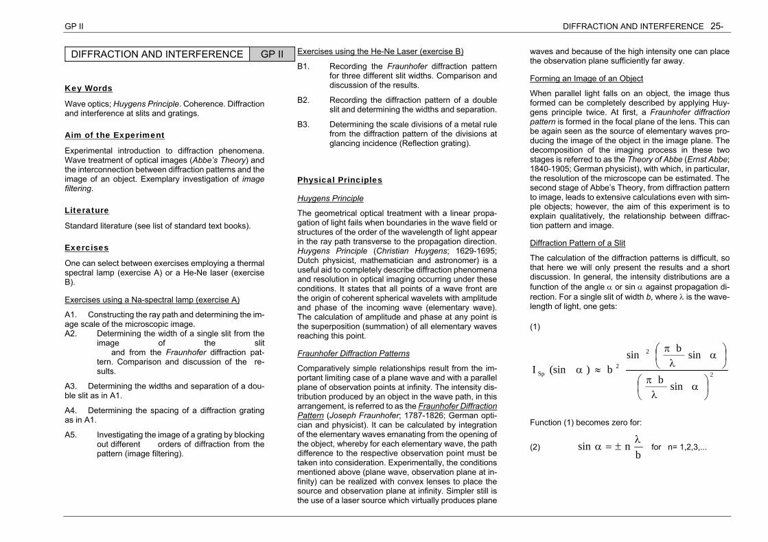
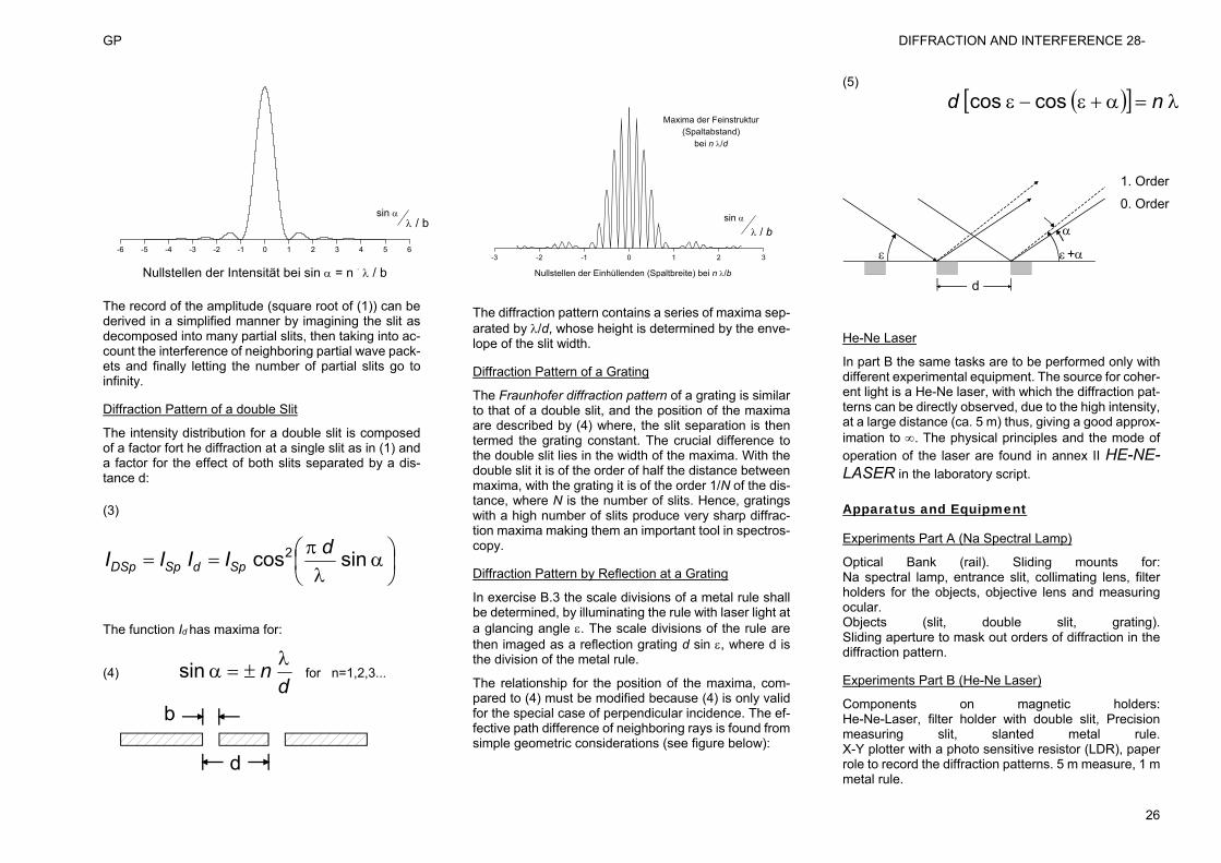
Diffraction Pattern of a Slit

The calculation of the diffraction patterns is difficult, so that here we will only present the results and a short discussion. In general, the intensity distributions are a function of the angle or sin against propagation di-rection. For a single slit of width b, where is the wave-length of light, one gets:

(1)

2

2

2Sp

sinb

sinbsinb)(sinI

Function (1) becomes zero for:

(2) b

nsin for n= 1,2,3,...

GP DIFFRACTION AND INTERFERENCE 28-

26

The record of the amplitude (square root of (1)) can be derived in a simplified manner by imagining the slit as decomposed into many partial slits, then taking into ac-count the interference of neighboring partial wave pack-ets and finally letting the number of partial slits go to infinity.

Diffraction Pattern of a double Slit

The intensity distribution for a double slit is composed of a factor fort he diffraction at a single slit as in (1) and a factor for the effect of both slits separated by a dis-tance d:

(3)

sincos2 dIIII SpdSpDSp

The function Id has maxima for:

(4) d

n sin for n=1,2,3...

The diffraction pattern contains a series of maxima sep-arated by /d, whose height is determined by the enve-lope of the slit width.

Diffraction Pattern of a Grating

The Fraunhofer diffraction pattern of a grating is similar to that of a double slit, and the position of the maxima are described by (4) where, the slit separation is then termed the grating constant. The crucial difference to the double slit lies in the width of the maxima. With the double slit it is of the order of half the distance between maxima, with the grating it is of the order 1/N of the dis-tance, where N is the number of slits. Hence, gratings with a high number of slits produce very sharp diffrac-tion maxima making them an important tool in spectros-copy.

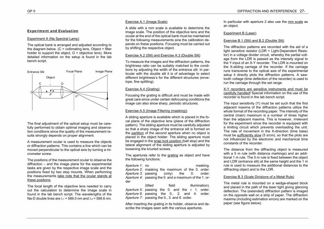
Diffraction Pattern by Reflection at a Grating

In exercise B.3 the scale divisions of a metal rule shall be determined, by illuminating the rule with laser light at a glancing angle . The scale divisions of the rule are then imaged as a reflection grating d sin , where d is the division of the metal rule.

The relationship for the position of the maxima, com-pared to (4) must be modified because (4) is only valid for the special case of perpendicular incidence. The ef-fective path difference of neighboring rays is found from simple geometric considerations (see figure below):

(5) nd coscos

1. Order

0. Order

+

d

He-Ne Laser

In part B the same tasks are to be performed only with different experimental equipment. The source for coher-ent light is a He-Ne laser, with which the diffraction pat-terns can be directly observed, due to the high intensity, at a large distance (ca. 5 m) thus, giving a good approx-imation to . The physical principles and the mode of operation of the laser are found in annex II HE-NE-LASER in the laboratory script.


Experiments Part A (Na Spectral Lamp)

Optical Bank (rail). Sliding mounts for: Na spectral lamp, entrance slit, collimating lens, filter holders for the objects, objective lens and measuring ocular. Objects (slit, double slit, grating). Sliding aperture to mask out orders of diffraction in the diffraction pattern.

Experiments Part B (He-Ne Laser)

Components on magnetic holders: He-Ne-Laser, filter holder with double slit, Precision measuring slit, slanted metal rule. X-Y plotter with a photo sensitive resistor (LDR), paper role to record the diffraction patterns. 5 m measure, 1 m metal rule.

-6 -5 -4 -3 -2 -1 0 1 2 3 4 5 6

/ bsin

Nullstellen der Intensität bei sin = n . / b-3 -2 -1 0 1 2 3

/ b

Nullstellen der Einhüllenden (Spaltbreite) bei n /b

Maxima der Feinstruktur(Spaltabstand)

bei n /d

sin

b

d

GP II DIFFRACTION AND INTERFERENCE 27-


Experiment A (Na Spectral Lamp)

The optical bank is arranged and adjusted according to the diagram below. (C = collimating lens, Object = filter holder to support the object, O = objective lens). More detailed information on the setup is found in the lab bench script.

C O

F'

Entrance Slit Focal Plane

F''

Object

Image Plane

The final adjustment of the optical setup must be care-fully performed to obtain optimal imaging and observa-tion conditions since the quality of the measurement re-sults strongly depends on proper alignment.

A measurement ocular is used to measure the objects or diffraction patterns. This contains a line which can be moved perpendicular to the optical axis by turning a mi-crometer screw.

The positions of the measurement ocular to observe the diffraction – and the image plane for the experimental tasks are given by the respective image scale and the positions fixed by two stop mounts. When performing the measurements take note that the ocular stands at these positions.

The focal length of the objective lens needed to carry out the calculation to determine the image scale in found in the lab bench script. The wavelengths of the Na-D double lines are 1 = 589.0 nm and 2 = 589.6 nm.

Exercise A.1 (Image Scale)

A slide with a mm scale is available to determine the image scale. The position of the objective lens and the ocular at the end of the optical bank must be maintained for the following measurements sine the calibration de-pends on these positions. Focusing must be carried out by shifting the respective object.

Exercise A.2 (Slit) and Exercise A.3 (Double Slit)

To measure the images and the diffraction patterns, the brightness ratio can be suitably matched to the condi-tions by adjusting the width of the entrance slit. In par-ticular with the double slit it is of advantage to select different brightness’s for the different structures (enve-lope, fine splitting).

Exercise A.4 (Grating)

Focusing the grating is difficult and must be made with great care since under certain defocusing conditions the image can also show sharp, periodic structures.

Exercise A.5 (Image Filtering (masking))

A sliding aperture is available which is placed in the fo-cal plane of the objective lens (plane of the diffraction pattern). The sliding aperture must be carefully adjusted so that a sharp image of the entrance slit is formed on the partition of the second aperture when no object is placed in the object holder. The sliding aperture must be engaged in the snap lock position (ball stop) and the lateral alignment of the sliding aperture is adjusted by loosening the knurled screws.

The apertures refer to the grating as object and have the following functions:

Aperture 1: no masking. Aperture 2: masking the maximum of the 0. order. Aperture 3: passing (only) the 0. order. Aperture 4: passing the 0. and a maximum of the 1. or-der (tilted field illumination). Aperture 5: passing the 0. and the 1. order. Aperture 6: passing the 0., 2. and 4. order. Aperture 7: passing the 0., 3. and 6. order.

After inserting the grating in its holder, observe and de-scribe the images seen with the various apertures.

In particular with aperture 2 also use the mm scale as an object.

Experiment B (Laser)

Exercise B.1 (Slit) and B.2 (Double Slit)

The diffraction patterns are recorded with the aid of a light sensitive resistor (LDR = Light-Dependent Resis-tor) in a voltage divider circuit, whereby the partial volt-age from the LDR is passed as the intensity signal to the Y-input of an X-Y recorder. The LDR is mounted on the X-sliding carriage of the recorder. If the carriage runs transverse to the optical axis of the experimental setup it directly plots the diffraction patterns. A saw-tooth voltage (time deflection of the recorder) is used to run the carriage through the set range.

X-Y recorders are sensitive instruments and must be carefully handled! Special information on the use of the recorder is found in the lab bench script.

The input sensitivity (Y) must be set such that the first adjacent maxima of the diffraction patterns utilize the whole format of the recording paper. The intensity of the central (main) maximum is a number of times higher than the adjacent maxima. This is however, irrelevant for the experiment since the recorder is equipped with a limiting circuit which prevents overloading the unit. The rate of movement in the X-direction (time base) must be sufficiently slow (5 s/cm), so that the plots are not influenced by the electronic and mechanical time constants of the recorder.

The distance from the diffracting object is measured with a 5 m rule (with distance markings) and an addi-tional 1 m rule. The 5 m rule is fixed between the object and LDR (entrance slit) at the same height and the 1 m rule is used to measure the additional distances to the diffracting object and to the LDR.

Exercise B.3 (Scale Divisions of a Metal Rule)

The metal rule is mounted on a wedge-shaped block and placed in the path of the laser light giving glancing deflection. The (extended) diffraction pattern is imaged on the opposite wall on a strip of paper. The diffraction maxima (including estimation errors) are marked on the paper (see figure below).

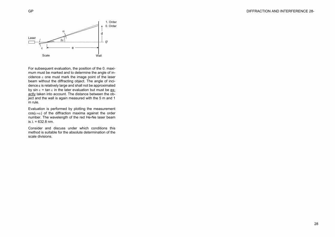
GP DIFFRACTION AND INTERFERENCE 28-

28

e

d

0'

Wall

Laser

Scale

1. Order0. Order

2

For subsequent evaluation, the position of the 0. maxi-mum must be marked and to determine the angle of in-cidence one must mark the image point of the laser beam without the diffracting object. The angle of inci-dence is relatively large and shall not be approximated by sin = tan in the later evaluation but must be ex-actly taken into account. The distance between the ob-ject and the wall is again measured with the 5 m and 1 m rule.

Evaluation is performed by plotting the measurement cos() of the diffraction maxima against the order number. The wavelength of the red He-Ne laser beam is = 632.8 nm.

Consider and discuss under which conditions this method is suitable for the absolute determination of the scale divisions.

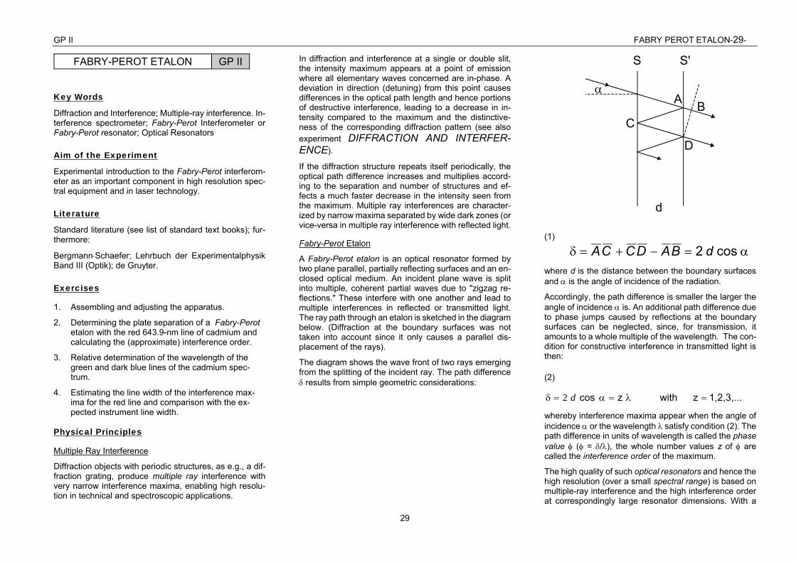
GP II FABRY PEROT ETALON-29-

29

FABRY-PEROT ETALON GP II

Key Words

Diffraction and Interference; Multiple-ray interference. In-terference spectrometer; Fabry-Perot Interferometer or Fabry-Perot resonator; Optical Resonators


Experimental introduction to the Fabry-Perot interferom-eter as an important component in high resolution spec-tral equipment and in laser technology.

Literature

Standard literature (see list of standard text books); fur-thermore:

BergmannSchaefer; Lehrbuch der Experimentalphysik Band III (Optik); de Gruyter.

Exercises

1. Assembling and adjusting the apparatus.

2. Determining the plate separation of a Fabry-Perot etalon with the red 643.9-nm line of cadmium and calculating the (approximate) interference order.

3. Relative determination of the wavelength of the green and dark blue lines of the cadmium spec-trum.

4. Estimating the line width of the interference max-ima for the red line and comparison with the ex-pected instrument line width.

Physical Principles

Multiple Ray Interference

Diffraction objects with periodic structures, as e.g., a dif-fraction grating, produce multiple ray interference with very narrow interference maxima, enabling high resolu-tion in technical and spectroscopic applications.

In diffraction and interference at a single or double slit, the intensity maximum appears at a point of emission where all elementary waves concerned are in-phase. A deviation in direction (detuning) from this point causes differences in the optical path length and hence portions of destructive interference, leading to a decrease in in-tensity compared to the maximum and the distinctive-ness of the corresponding diffraction pattern (see also experiment DIFFRACTION AND INTERFER-ENCE).

If the diffraction structure repeats itself periodically, the optical path difference increases and multiplies accord-ing to the separation and number of structures and ef-fects a much faster decrease in the intensity seen from the maximum. Multiple ray interferences are character-ized by narrow maxima separated by wide dark zones (or vice-versa in multiple ray interference with reflected light.

Fabry-Perot Etalon

A Fabry-Perot etalon is an optical resonator formed by two plane parallel, partially reflecting surfaces and an en-closed optical medium. An incident plane wave is split into multiple, coherent partial waves due to "zigzag re-flections." These interfere with one another and lead to multiple interferences in reflected or transmitted light. The ray path through an etalon is sketched in the diagram below. (Diffraction at the boundary surfaces was not taken into account since it only causes a parallel dis-placement of the rays).

The diagram shows the wave front of two rays emerging from the splitting of the incident ray. The path difference results from simple geometric considerations:

S S'

A B

C

D

d

(1)

cos 2 dBADCCA

where d is the distance between the boundary surfaces and is the angle of incidence of the radiation.

Accordingly, the path difference is smaller the larger the angle of incidence is. An additional path difference due to phase jumps caused by reflections at the boundary surfaces can be neglected, since, for transmission, it amounts to a whole multiple of the wavelength. The con-dition for constructive interference in transmitted light is then:

(2)

1,2,3,...z with zcos d2

whereby interference maxima appear when the angle of incidence or the wavelength satisfy condition (2). The path difference in units of wavelength is called the phase value ( = /), the whole number values z of are called the interference order of the maximum.

The high quality of such optical resonators and hence the high resolution (over a small spectral range) is based on multiple-ray interference and the high interference order at correspondingly large resonator dimensions. With a

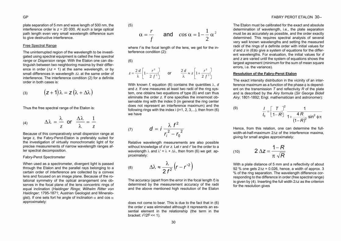
GP FABRY PEROT ETALON 30--

30

plate separation of 5 mm and wave length of 500 nm, the interference order is z = 20 000. At such a large optical path length even very small wavelength difference sum to give destructive interference.

Free Spectral Range

The uninterrupted region of the wavelength to be investi-gated using spectral equipment is called the free spectral range or Dispersion range. With the Etalon one can dis-tinguish between two neighboring maxima by their differ-ence in order (z = 1) at the same wavelength, or by small differences in wavelength at the same order of interference. The interference condition (2) for a definite order in both cases is:

(3) zz 1

Thus the free spectral range of the Etalon is:

(4) zz1

or

Because of this comparatively small dispersion range at large z, the Fabry-Perot-Etalon is preferably suited for the investigation of virtually monochromatic light of for precise measurements of narrow wavelength ranges af-ter spectral decomposition.

Fabry-Perot Spectrometer

When used as a spectrometer, divergent light is passed through the Etalon and the parallel rays belonging to a certain order of interference are collected by a convex lens and focused on an image plane. Because of the ro-tational symmetry of the optical arrangement one ob-serves in the focal plane of the lens concentric rings of equal inclination (Haidinger Rings; Wilhelm Ritter von Haidinger; 1795-1871; Austrian Geologist and Mineralo-gist). If one sets fort he angle of inclination and cos approximately:

(5)

2

211 cos

fr and

where f is the focal length of the lens, we get for the in-terference condition (2):

(6)

2

2

2

2

212

212

frzd

frdz or

With known f, equation (6) contains the quantities , d and z. If one measures at least two radii of the ring sys-tem, one obtains two equations of type (6) and can thus eliminate the order z. If one specifies the innermost ob-servable ring with the index 0 (in general the ring center does not represent an interference maximum) and the following rings with the index i (i=1, 2, 3,...), then from (6) we have

(7) 20

2

2

rrfid

i

Relative wavelength measurements are also possible without knowledge of d or z. Let r and r' be the order to a wavelength and ' = + , then from (6) we get ap-proximately:

(8) 22 `

2rr

f

The accuracy (apart from the error in the focal length f) is determined by the measurement accuracy of the radii and the above mentioned high resolution of the Etalon

does not come to bear. This is due to the fact that in (6) the order z was eliminated although it represents an es-sential element in the relationship (the term in the bracket: r2/2f2 << 1).

The Etalon must be calibrated for the exact and absolute determination of wavelength, i.e., the plate separation must be as accurately as possible, and the order exactly determined. This requires spectral analysis of several very well known wavelengths and setting the measured radii of the rings of a definite order with initial values for d and z in (6)to give a system of equations for the differ-ent wavelengths. For evaluation, the initial values for d and z are varied until the system of equations shows the largest agreement (minimum for the sum of mean square errors, i.e. the variance).

Resolution of the Fabry-Perot Etalon

The exact intensity distribution in the vicinity of an inter-ference maximum as a function of the phase is depend-ent on the transmission T and reflectivity R of the plate and is described by the Airy formula (Sir George Bidell Airy; 1801-1892; Engl. mathematician and astronomer):

(9)

2

2

2

0 sin1

41

11

RRR

TII

Hence, from this relation, one can determine the full-width-at-half-maximum 2z of the interference maxima, giving for small angles approximately:

(10) RRz

12

With a plate distance of 5 mm and a reflectivity of about 92 % one gets 2z = 0.026, hence, a width of approx. 3 % of the ring separation. The wavelength difference cor-responding to the difference in order (free spectral range) is given by (4). Inserting the full width 2z as the criterion for the resolution gives

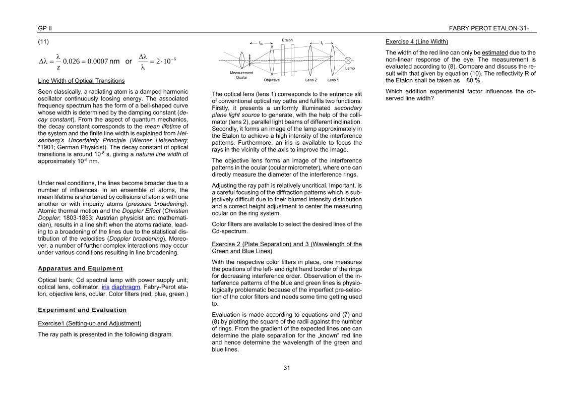
GP II FABRY PEROT ETALON-31-

31

(11)

6102000700260

or nm ..z

Line Width of Optical Transitions

Seen classically, a radiating atom is a damped harmonic oscillator continuously loosing energy. The associated frequency spectrum has the form of a bell-shaped curve whose width is determined by the damping constant (de-cay constant). From the aspect of quantum mechanics, the decay constant corresponds to the mean lifetime of the system and the finite line width is explained from Hei-senberg’s Uncertainty Principle (Werner Heisenberg; *1901; German Physicist). The decay constant of optical transitions is around 10-8 s, giving a natural line width of approximately 10-5 nm.

Under real conditions, the lines become broader due to a number of influences. In an ensemble of atoms, the mean lifetime is shortened by collisions of atoms with one another or with impurity atoms (pressure broadening). Atomic thermal motion and the Doppler Effect (Christian Doppler; 1803-1853; Austrian physicist and mathemati-cian), results in a line shift when the atoms radiate, lead-ing to a broadening of the lines due to the statistical dis-tribution of the velocities (Doppler broadening). Moreo-ver, a number of further complex interactions may occur under various conditions resulting in line broadening.


Optical bank; Cd spectral lamp with power supply unit; optical lens, collimator, iris diaphragm, Fabry-Perot eta-lon, objective lens, ocular. Color filters (red, blue, green.)


Exercise1 (Setting-up and Adjustment)

The ray path is presented in the following diagram.

Objective

Etalon

Lamp

Lens 2 Lens 1

MeasurementOcular

fOb f2

The optical lens (lens 1) corresponds to the entrance slit of conventional optical ray paths and fulfils two functions. Firstly, it presents a uniformly illuminated secondary plane light source to generate, with the help of the colli-mator (lens 2), parallel light beams of different inclination. Secondly, it forms an image of the lamp approximately in the Etalon to achieve a high intensity of the interference patterns. Furthermore, an iris is available to focus the rays in the vicinity of the axis to improve the image.

The objective lens forms an image of the interference patterns in the ocular (ocular micrometer), where one can directly measure the diameter of the interference rings.

Adjusting the ray path is relatively uncritical. Important, is a careful focusing of the diffraction patterns which is sub-jectively difficult due to their blurred intensity distribution and a correct height adjustment to center the measuring ocular on the ring system.

Color filters are available to select the desired lines of the Cd-spectrum.

Exercise 2 (Plate Separation) and 3 (Wavelength of the Green and Blue Lines)

With the respective color filters in place, one measures the positions of the left- and right hand border of the rings for decreasing interference order. Observation of the in-terference patterns of the blue and green lines is physio-logically problematic because of the imperfect pre-selec-tion of the color filters and needs some time getting used to.

Evaluation is made according to equations and (7) and (8) by plotting the square of the radii against the number of rings. From the gradient of the expected lines one can determine the plate separation for the „known“ red line and hence determine the wavelength of the green and blue lines.

Exercise 4 (Line Width)

The width of the red line can only be estimated due to the non-linear response of the eye. The measurement is evaluated according to (8). Compare and discuss the re-sult with that given by equation (10). The reflectivity R of the Etalon shall be taken as 80 %.

Which addition experimental factor influences the ob-served line width?

GP SPECIFIC CHARGE e/m OF THE ELECTRON 32--

32

SPECIFIC CHARGE e/m0 of the Electron GP II

Key Words

Specific charge and charge quantization. Lorentz force. Circular motion.

Aim of the Experiment Exemplary experiment on the atomic structure of elec-tricity and measurement methods by the deflection of charged particles in orthogonal electric and magnetic fields.

Literature

Gerthsen Physik (22. Auflage): 8.1.1, 8.2 Bergmann-Schaefer, Band 2 (8. Auflage): 3.4.4, 7.1.2, 11.1.7, 11.1.4 , 11.3.5

Suplementary: Bergmann Schäfer; Experimentalphysik Band II: de Gruyter. Geiger, Scheel: Handbuch der Physik XXII. (Histor-ische, vertiefende Anmerkungen)

Exercise

Determining the specific charge of the electron e/m o by measuring the magnetic deflection of electrons in a nar-row beam tube.

Physical Principles

At the beginning of the 19th. centaury results of physical experiments showed clear indications for a corpuscular nature of the electric charge. The experiments of Fara-day (Michael Faraday; 1791-1867; Eng. physicist and chemist) and the laws of electrolysis gave a definite re-lationship between the amount of electricity and the mass of the carrier of electricity and allowed, together with the idea of an atomic structure of material, the con-clusion of the quantized nature of charge. Helmholtz (Hermann von Helmholtz; 1821-1894; Ger. physicist and physiologist) talked in a Faraday commemoration speech 1881 about the "the electric charge of the ion" and said "just the same certain amount, let it be positive or negative

electricity moves with each single valued ion or with each valence of a multi-valued ion, and accompanies it insepara-bly in all movements the ions make through the liquid. If car-ried over to the electrical processes, this hypothesis, leads, in connection with Faraday’s law, to a somewhat surprising conclusion. If we assume atoms of chemical elements, then we must conclude that also electricity, positive as well as negative, is divided into certain elementary quanta which be-have as atoms of electricity." The electrolytic measure-ments, however, only gave mol values for ions, so that the determination of the specific charge and the ion charge presupposed the knowledge of Loschmidt’s number.

The story of the discovery of the electron began in 1860 with the investigation of gas discharges and the discov-ery of cathode rays by Plücker 1859 (Julius Plücker; 1801-1868; German physicist and mathematician). Hit-torf (Johann Wilhelm Hittorf; 1824-1914; German physicist and chemist) discovered in 1869 the magnetic- and Goldstein (Eugen Goldstein; 1850-1930; German physi-cist) in 1876 the electric deflection of cathode rays, whereby, Hittorf already suspected negatively charge particles were the actual physical nature of the cathode rays. Around 1890 Schuster (K. Schuster; *1903), Thom-son (Sir Joseph John Thomson; 1856-1940; Engl. physi-cist) and Wiechert (Emil Wiechert; 1861-1928; German Geophysicist) performed the first measurements of the specific charge in various deflection experiments. Even though the early results of these measurements had large errors, it was found that "the mass of the cathode rays must be about 2000 times smaller than that of the light-est ions." Extensive measurements of the velocity (Thomson) and investigations on the velocity depend-ence of the mass and the agreement of the specific charge of the cathode rays with those of electrons re-leased by photoelectric or thermal effects gave certainty to the existence of electrons. Thomson is named as the classical discoverer.

At the beginning of the 20th. centaury the value of the electron charge itself was measured ( Millikan 1910-1925; see MILLIKAN Experiment in the laboratory script ) and, especially due to the determination of the specific charge from the Zeeman Effect ( Pieter Zee-man; 1865-1943; Dutch physicist ) and from the Ry-dberg Constant ( Johannes Rydberg; 1854-1919;

Swed. physicist; see experiment OPTICAL SPEC-TROSCOPY in this laboratory script ), the identity be-tween the free electrons and the bound electrons as building blocks of atoms was proven.

The recommended values for the electron (CODATA 1999) are ( Physikalische Blätter, March 2000 ):

(1a) e/mo = 1.758820174 .1011 C/kg relative error: 1.2 .10-7

(1b) e = 1.602176462(63) .10-19 C relative error: 3.9 .10-8

(1c) mo = 9.10938188(72) .10-31 kg relative error: 7.9 .10-8

If one interprets the total rest mass of the electron ac-cording to Einstein’s equation (E = mc2) as the electro-static energy content of spherical charge distribution of radius r, then we have:

(2) r0

22

0 8

ecm

(E = CU2/2 with C = 4or). Solving for r and inserting the respective values gives r = 1.410-15 m. This value at least reflects correctly the order of magnitude of the electron radius as supported by deflection experiments, even when from the stand point of quantum physics it is basically unfounded to describe or explain the electron with classical concepts. In the literature it is usual to take the double value of (2) as the classical electron radius:

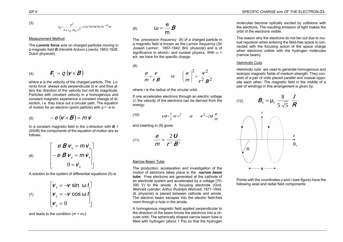
GP II SPECIFIC CHARGE e/m OF THE ELECTRON-33-

(3) m

cme 1510)70(8179378.2

2004

20

r

Measurement Method

The Lorentz force acts on charged particles moving in a magnetic field B (Hendrik Antoon Lorentz; 1853-1928; Dutch physicist):

(4) Bv qLF

where v is the velocity of the charged particle. The Lo-rentz force always acts perpendicular to v; and thus al-ters the direction of the velocity but not its magnitude. Particles with constant velocity in a homogenous and constant magnetic experience a constant change of di-rection, i.e. they trace out a circular path. The equation of motion for an electron (point particle) with q = -e is:

(5) vBv me

In a constant magnetic field in the z-direction with B = (0/0/B) the components of the equation of motion are as follows:

(6)

z

xy

yx

vvvBvvB

0

mm

ee

A solution to the system of differential equations (5) is

(7)

0z

y

x

ω cos ω sin

vvvvv

tt

and leads to the condition (m = mo):

(8) Bmeω

The precession frequency (8) of a charged particle in a magnetic field is known as the Larmor frequency (Sir Joseph Larmor; 1857-1942; Brit. physicist) and is of significance in atomic- and nuclear physics. With = v/r, we have for the specific charge:

(9)

22

22or

Brv

Brv

me

me

where r is the radius of the circular orbit.

If one accelerates electrons through an electric voltage U, the velocity of the electrons can be derived from the energy:

(10) mem UvU 22 2v

21

or e

and inserting in (9) gives:

(11) 22

2BrU

me

Narrow Beam Tube

The production, acceleration and investigation of the motion of electrons takes place in the narrow beam tube. Free electrons are generated at the cathode of an electrode system and accelerated by a voltage (70-300 V) to the anode. A focusing electrode (Grid, Wehnelt cylinder; Arthur Rudolph Wehnelt; 1871-1944; dt. physicist) is placed between cathode and anode. The electron beam escapes into the electric field-free room through a hole in the anode.

A homogenous magnetic field applied perpendicular to the direction of the beam forces the electrons into a cir-cular orbit. The spherically shaped narrow beam tube is filled with hydrogen (about 1 Pa) so that the hydrogen

molecules become optically excited by collisions with the electrons. The resulting emission of light makes the orbit of the electrons visible.

The reason why the electrons do not fan out due to mu-tual repulsion when entering the field-free space is con-nected with the focusing action of the space charge when electrons collide with the hydrogen molecules (narrow beam).

Helmholtz Coils

Helmholtz coils are used to generate homogenous and isotropic magnetic fields of medium strength. They con-sists of a pair of coils placed parallel and coaxial oppo-site each other. The magnetic field in the middle of a pair of windings in this arrangement is given by:

(12) RIB μ

558

00

r

z

zBR

R

Points with the coordinates z and r (see figure) have the following axial and radial field components:

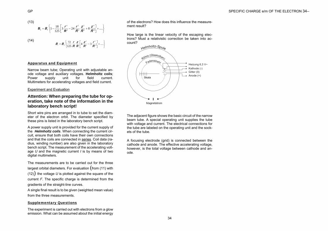
GP SPECIFIC CHARGE e/m OF THE ELECTRON 34--

34

(13)

....z 4

4

2

2

2

2

4

4

0 8243125181

Rz

Rz

RrrB

RB

(14)

....r 2

2

2

2

0 3412572

Rr

Rz

Rz

RrBB


Narrow beam tube; Operating unit with adjustable an-ode voltage and auxiliary voltages. Helmholtz coils; Power supply unit for field current. Multimeters for accelerating voltages and field current.


Attention: When preparing the tube for op-eration, take note of the information in the laboratory bench script! Short wire pins are arranged in to tube to set the diam-eter of the electron orbit. The diameter specified by these pins is listed in the laboratory bench script.

A power supply unit is provided for the current supply of the Helmholtz coils. When connecting the current cir-cuit, ensure that both coils have their own connections and that the coils are connected in series. Coil data (ra-dius, winding number) are also given in the laboratory bench script. The measurement of the accelerating volt-age U and the magnetic current I is by means of two digital multimeters.

The measurements are to be carried out for the three largest orbital diameters. For evaluation (from (11) with (12)) the voltage U is plotted against the square of the current I2. The specific charge is determined from the gradients of the straight-line curves. A single final result is to be given (weighted mean value) from the three measurements.

Supplementary Questions

The experiment is carried out with electrons from a glow emission. What can be assumed about the initial energy

of the electrons? How does this influence the measure-ment result?

How large is the linear velocity of the escaping elec-trons? Must a relativistic correction be taken into ac-count?

Heizung 6,3 V~Kathode (-)Gitter (0)Anode (+)

The adjacent figure shows the basic circuit of the narrow beam tube. A special operating unit supplies the tube with voltage and current. The electrical connections for the tube are labeled on the operating unit and the sock-ets of the tube.

A focusing electrode (grid) is connected between the cathode and anode. The effective accelerating voltage, however, is the total voltage between cathode and an-ode.

GP II MILLIKAN-EXPERIMENT -35-

MILLIKAN EXPERIMENT GP II

Key Words

Charge quantization, elementary charge. Coulomb force; Stokes’ Law.


Simple and exemplary experiment to verify and meas-ure quantized values.

Literature

Bergmann-Schaefer, Band 2 (8. Auflage), Kapitel 7.1.2

Exercise

Determining the elementary charge from the measure-ments of the fall- and rise times of charged droplets of oil of various sizes, taking into account a radius depend-ent correction.

Physical Principles

Charge Quantization

After the discovery of electrical phenomena, people be-gan, in the middle of the 18th. centaury, to make scien-tific enquiries as to the nature of electricity. The predom-inant theories at this time were fluid theories, although others argued for a more simple, mechanical world view, as e.g. Franklin (Benjamin Franklin; 1706-1790; Am. politician, writer and natural scientist), who imag-ined electricity to consists of small particles able to move through materials without hindrance.

Already in 1833 Faraday (Michael Faraday; 1791-1867; Eng. physicist and chemist) discovered, with his laws of electrolysis, the first experimental evidence for an atom-istic nature of electricity without, however, (him and other physicist of the time) recognizing the quantization of charge. Only in the seventies and eighties of the last centaury did Stoney (George Johnstone Stoney; 1826-1911; Eng. physicist) and Helmholtz (Hermann von Helmholtz; 1821-1894; Ger. physicist and physiologist)

formulate in all clarity that "electricity is made up of cer-tain, elementary quanta, which behave as atoms of electricity".

Electrolytic measurements only gave values related to mass, such as eo/mI or Leo (elementary quantum of charge eo, ion mass mI, Avogadro’s number L). The first values of the ion charge were found through independ-ent experiments to determine the constant L. Since these experiments were fraught with difficulties, others were conceived in which the number of charge carriers could be directly counted. The charge carriers used were individual atomic ions (-particles) as well as ions attached to liquid droplets (ion-cloud method). In addi-tion, experiments were performed to determine the ion charge from radioactive decay data.

The further developments of the cloud- and droplet method lead to charge measurements on single, iso-lated particles. The leading working groups were those of F. Ehrenhaft (Felix Ehrenhaft; 1879-1952; Austrian physicist) in Vienna and R. A. Millikan (Robert Andrews Millikan; 1868-1953; Am. physicist) in Chicago. Both groups worked from 1910 onwards with the method de-scribed below. The two necessary measurements (in field-free space and under the influence of an electric field) were carried on one and the same particle.

While Millikan tried to prove the existence of the ele-mentary charge qualitatively and quantitatively, Ehren-haft was not convinced of the notion of an elementary quantum and the aim of his work was to disprove this concept. Millikan published his essential work in 1911 and 1913 and carried on till the middle of the twenties to systematically improve his results. Millikan’s last, in 1925, published result was (converted to in SI-units):

(1) eo = 1.5924(17)10-19 C

The importance of Millikan’s work lies in a direct and simple qualitative and quantitative proof of charge quantization. In 1923 he received the Noble prize in physics for these measurements and for the experi-mental confirmation of Einstein’s equation E = h·.

Today, the existence of the elementary charge is be-yond doubt even when considerations are given to the existence of fundamental particles with the charge 1/3 eo and 2/3 eo (Quarks). Furthermore, the elementary charge seems to have the same magnitude for all

known elementary particles. In experiments, the relative difference between electrons and protons was found to be less than 10-20. At present, the elementary charge is determined indirectly from other experimental data. In 1999 CODATA recommended the following value (Physikalische Blätter 2000):

(1a) eo = 1.602176462(63)10-19 C

relative error: 3.9 10-8.

Measurement Method

Four forces act on a spherical, charged body (here, a small droplet of oil) placed in a vertical, homogenous and constant electric field and within a homogenous medium: the force of gravity FG, the force of buoyancy FA, the Coulomb force FC (Charles Augustin de Cou-lomb; 1736-1806; French physicist) and a frictional force FR. If laminar flow is assumed, the frictional force is given by Stokes’ Law (Sir George Gabriel Stokes; 1819-1903; Engl. mathematician and physicist):

(2) vrFR 6

is the viscosity, r the radius of the droplet and v its velocity. Because of the velocity dependence, the fric-tional force compensates the other forces after a suffi-cient time and one observes a force-free uniform mo-tion. One can thus calculate the radius of the droplet by measuring its velocity when falling in field-free space.

If one now applies an electric field (e.g. between two capacitor plates), so that the droplet rises, one can then calculate the charge q of the droplet from the radius and rise velocity.

The experimental setup consists of a plate capacitor, an atomizer to produce fine droplets of oil, illuminating equipment and a measuring microscope to observe the droplets (see figure).

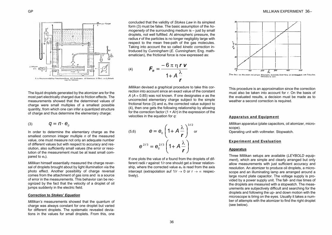
GP MILLIKAN EXPERIMENT 36--

36

The liquid droplets generated by the atomizer are for the most part electrically charged due to friction effects. The measurements showed that the determined values of charge were small multiples of a smallest possible quantity, from which one can infer a quantized structure of charge and thus determine the elementary charge:

(3) 0enq

In order to determine the elementary charge as the smallest common integer multiple n of the measured value, one must measure not only an adequate number of different values but with respect to accuracy and res-olution, also sufficiently small values (the error or reso-lution of the measurement must be at least small com-pared to eo).

Millikan himself essentially measured the charge rever-sal of droplets brought about by light illumination via the photo effect. Another possibility of charge reversal comes from the attachment of gas ions and is a source of error in the measurements. This behavior can be rec-ognized by the fact that the velocity of a droplet of oil jumps suddenly in the electric field.

Correction to Stokes’ Equation

Millikan’s measurements showed that the quantum of charge was always constant for one droplet but varied for different droplets. The systematic revealed devia-tions in the values for small droplets. From this, one

concluded that the validity of Stokes Law in its simplest form (3) must be false. The basic assumption of the ho-mogeneity of the surrounding medium is – just by small droplets, not well fulfilled. At atmospheric pressure, the radius r of the particles is no longer negligibly large with respect to the mean free-path of the gas molecules. Taking into account the so called kinetic correction in-troduced by Cunningham (E. Cunningham; Eng. math-ematician), the frictional force is now expressed as:

(4)

r

vrFR

A

1

6

Millikan devised a graphical procedure to take this cor-rection into account since an exact value of the constant A (A 0.85) was not known. If one designates e as the uncorrected elementary charge subject to the simple frictional force (3) and eo the corrected value subject to (4), then one gets the following relationship by allowing for the correction factor (1 + A/r) in the expression of the velocities in the equation for q:

(5,6)

23

0 1/

r

Aee or

r// Aee 132

032

If one plots the value of e found from the droplets of dif-ferent radii r against 1/r one should get a linear relation-ship, where the corrected value eo is read from the axis intercept (extrapolation auf 1/r 0 or r respec-tively).

This procedure is an approximation since the correction must also be taken into account for r. On the basis of the evaluated results, a decision must be made as to weather a second correction is required.


Millikan apparatus (plate capacitors, oil atomizer, micro-scope). Operating unit with voltmeter. Stopwatch.


Apparatus

Three Millikan setups are available (LEYBOLD equip-ment), which are simple and clearly arranged but only allow measurements with just sufficient accuracy and resolution. An atomizer to produce oil droplets, a micro-scope and an illuminating lamp are arranged around a large round plate capacitor. The voltage supply is pro-vided by a power supply unit. The fall- and rise times of the droplets are measured with a stopwatch. The meas-urements are subjectively difficult and searching for the droplets and following the up- and down motion with the microscope is tiring on the eyes. Usually it takes a num-ber of attempts with the atomizer to find the right droplet (see below).

GP II MILLIKAN-EXPERIMENT -37-

An additional experimental setup is available from Pasco-Scientific which allows much better measure-ments.

Producing and Selecting the Droplets

Droplets of suitable charge and size must be selected from the mist produced by the atomizer. In general, large droplets carry a high charge and are therefore un-suitable for the detection of quantization and the deter-mination of the elementary charge. Large drops can be recognized by a large falling velocity without an electric field.

When looking through the microscope, falling droplets "rise" in field-free space because of image reversal. When the voltage is switched on, the droplets must move in the opposite direction. With the LEYBOLD ap-paratus one selects from these droplets those that have a falling velocity of less than 0.5-1 scale division/s. This may require some effort since the atomizer produces mainly large droplets. More information is given in the lab bench script.

Evaluation of the measurements, taking into account the radius dependent correction according to equation (6) requires measurement data for droplets of different radii.

Measurements

The measurements consist of collecting fall-and rise time data of droplets traveling a given distance. The measurements must take into account the required ac-curacy and the possibility of checking and reproducing the results.

Of all the data needed for evaluation, the capacitor volt-age contributes the largest and thus the decisive error. The voltage is adjustable and measured with an instru-ment of quality class 2.5.The time measurements should be made such that the total error does not in-crease significantly.

The fall- and rise times of a droplet must be repeatedly measured to increase the accuracy and to check the er-ror and the reproducibility. A compromise must be made with respect to the voltage. A large voltage gives a small (relative) voltage error, but a larger time error due to the short rise time and vice versa.

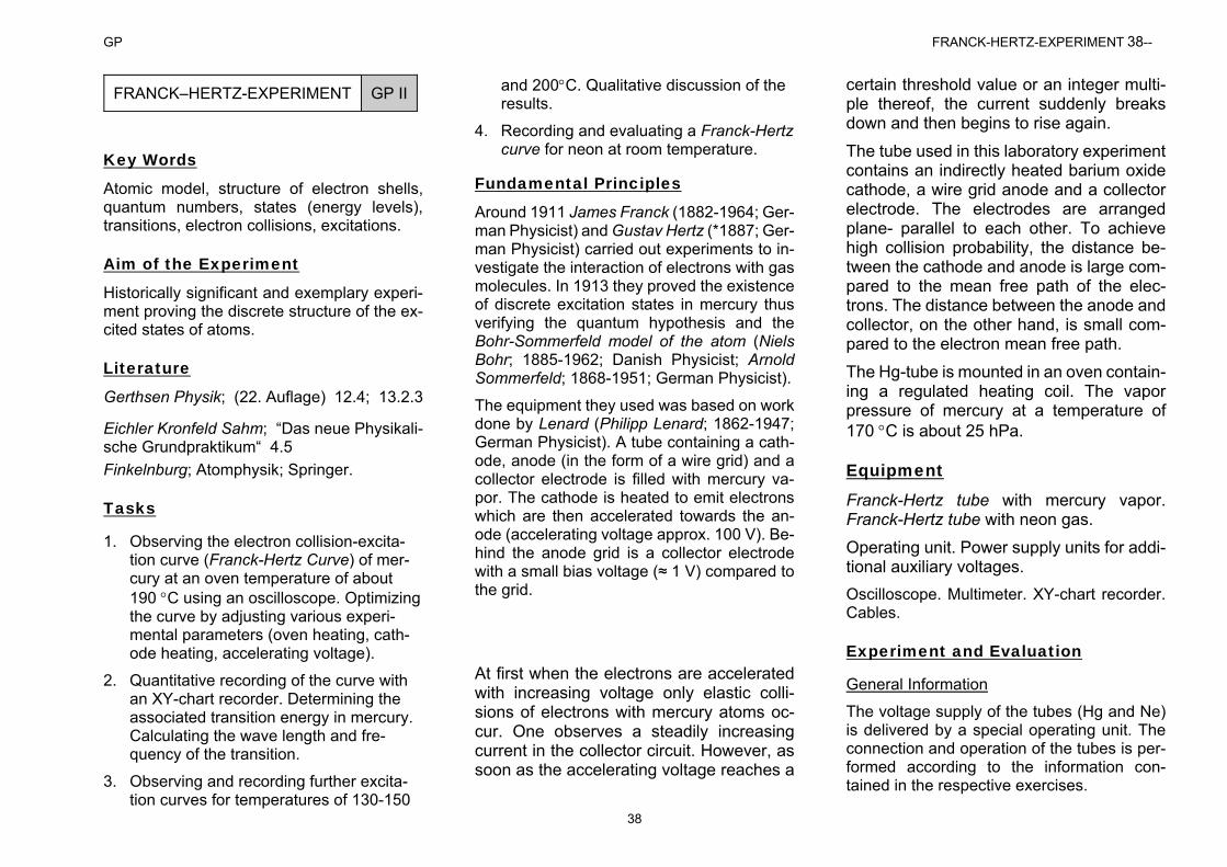
GP FRANCK-HERTZ-EXPERIMENT 38--

38

FRANCK–HERTZ-EXPERIMENT GP II

Key Words

Atomic model, structure of electron shells, quantum numbers, states (energy levels), transitions, electron collisions, excitations.


Historically significant and exemplary experi-ment proving the discrete structure of the ex-cited states of atoms.

Literature

Gerthsen Physik; (22. Auflage) 12.4; 13.2.3

Eichler Kronfeld Sahm; “Das neue Physikali-sche Grundpraktikum“ 4.5 Finkelnburg; Atomphysik; Springer.

Tasks

1. Observing the electron collision-excita-tion curve (Franck-Hertz Curve) of mer-cury at an oven temperature of about 190 C using an oscilloscope. Optimizing the curve by adjusting various experi-mental parameters (oven heating, cath-ode heating, accelerating voltage).

2. Quantitative recording of the curve with an XY-chart recorder. Determining the associated transition energy in mercury. Calculating the wave length and fre-quency of the transition.

3. Observing and recording further excita-tion curves for temperatures of 130-150

and 200C. Qualitative discussion of the results.

4. Recording and evaluating a Franck-Hertz curve for neon at room temperature.

Fundamental Principles

Around 1911 James Franck (1882-1964; Ger-man Physicist) and Gustav Hertz (*1887; Ger-man Physicist) carried out experiments to in-vestigate the interaction of electrons with gas molecules. In 1913 they proved the existence of discrete excitation states in mercury thus verifying the quantum hypothesis and the Bohr-Sommerfeld model of the atom (Niels Bohr; 1885-1962; Danish Physicist; Arnold Sommerfeld; 1868-1951; German Physicist).

The equipment they used was based on work done by Lenard (Philipp Lenard; 1862-1947; German Physicist). A tube containing a cath-ode, anode (in the form of a wire grid) and a collector electrode is filled with mercury va-por. The cathode is heated to emit electrons which are then accelerated towards the an-ode (accelerating voltage approx. 100 V). Be-hind the anode grid is a collector electrode with a small bias voltage (≈ 1 V) compared to the grid.

At first when the electrons are accelerated with increasing voltage only elastic colli-sions of electrons with mercury atoms oc-cur. One observes a steadily increasing current in the collector circuit. However, as soon as the accelerating voltage reaches a

certain threshold value or an integer multi-ple thereof, the current suddenly breaks down and then begins to rise again.

The tube used in this laboratory experiment contains an indirectly heated barium oxide cathode, a wire grid anode and a collector electrode. The electrodes are arranged plane- parallel to each other. To achieve high collision probability, the distance be-tween the cathode and anode is large com-pared to the mean free path of the elec-trons. The distance between the anode and collector, on the other hand, is small com-pared to the electron mean free path.

The Hg-tube is mounted in an oven contain-ing a regulated heating coil. The vapor pressure of mercury at a temperature of 170 C is about 25 hPa.

Equipment

Franck-Hertz tube with mercury vapor. Franck-Hertz tube with neon gas.

Operating unit. Power supply units for addi-tional auxiliary voltages. Oscilloscope. Multimeter. XY-chart recorder. Cables.


General Information

The voltage supply of the tubes (Hg and Ne) is delivered by a special operating unit. The connection and operation of the tubes is per-formed according to the information con-tained in the respective exercises.

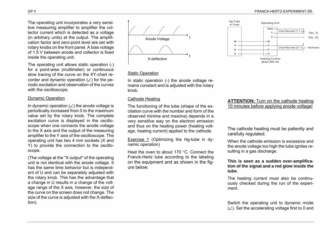
GP II FRANCK-HERTZ-EXPERIMENT-39-

The operating unit incorporates a very sensi-tive measuring amplifier to amplifier the col-lector current which is detected as a voltage (in arbitrary units) at the output. The amplifi-cation factor and zero-point level are set with rotary knobs on the front panel. A bias voltage of 1.5 V between anode and collector is fixed inside the operating unit.

The operating unit allows static operation (-) for a point-wise (multimeter) or continuous slow tracing of the curve on the XY-chart re-corder and dynamic operation () for the pe-riodic excitation and observation of the curves with the oscilloscope.

Dynamic Operation

In dynamic operation () the anode voltage is periodically increased from 0 to the maximum value set by the rotary knob. The complete excitation curve is displayed in the oscillo-scope when one connects the anode voltage to the X axis and the output of the measuring amplifier to the Y axis of the oscilloscope. The operating unit has two 4 mm sockets (X and Y) to provide the connection to the oscillo-scope.

(The voltage at the "X output" of the operating unit is not identical with the anode voltage. It has the same time behavior but is independ-ent of U and can be separately adjusted with the rotary knob. This has the advantage that a change in U results in a change of the volt-age range of the X axis, however, the size of the curve on the screen does not change. The size of the curve is adjusted with the X-deflec-tion).

t

t

Anode Voltage

X-deflection

Static Operation

In static operation (-) the anode voltage re-mains constant and is adjusted with the rotary knob.

Cathode Heating

The functioning of the tube (shape of the ex-citation curve with the number and form of the observed minima and maxima) depends in a very sensitive way on the electron emission and thus on the heating power (heating volt-age, heating current) applied to the cathode.

Exercise 1 (Optimizing the Hg-tube in dy-namic operation)

Heat the oven to about 170 C. Connect the Franck-Hertz tube according to the labeling on the equipment and as shown in the fig-ure below:

K

AM

H

-

+

Heating Currentabout 200 mA

K

AM

H

blueYX

Osc. (I)

Osc. (II)

Chart Recorder (Y = IA)

Chart Recorder (X = UA) / Multimeter

+

-

Operating UnitHg-Tubein Oven

ATTENTION: Turn on the cathode heating 10 minutes before applying anode voltage!

The cathode heating must be patiently and carefully regulated. When the cathode emission is excessive and the anode voltage too high the tube ignites re-sulting in a gas discharge. This is seen as a sudden over-amplifica-tion of the signal and a red glow inside the tube. The heating current must also be continu-ously checked during the run of the experi-ment.

Switch the operating unit to dynamic mode (). Set the accelerating voltage first to 0 and

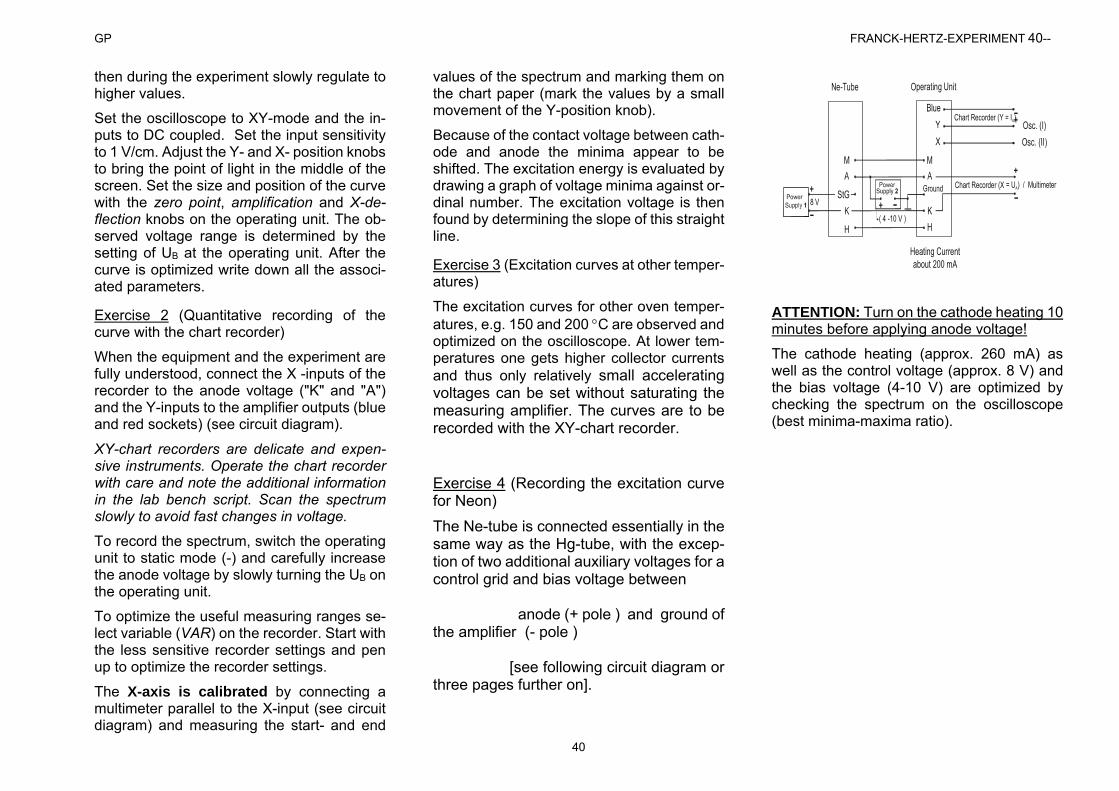
GP FRANCK-HERTZ-EXPERIMENT 40--

40

then during the experiment slowly regulate to higher values.

Set the oscilloscope to XY-mode and the in-puts to DC coupled. Set the input sensitivity to 1 V/cm. Adjust the Y- and X- position knobs to bring the point of light in the middle of the screen. Set the size and position of the curve with the zero point, amplification and X-de-flection knobs on the operating unit. The ob-served voltage range is determined by the setting of UB at the operating unit. After the curve is optimized write down all the associ-ated parameters.

Exercise 2 (Quantitative recording of the curve with the chart recorder)

When the equipment and the experiment are fully understood, connect the X -inputs of the recorder to the anode voltage ("K" and "A") and the Y-inputs to the amplifier outputs (blue and red sockets) (see circuit diagram).

XY-chart recorders are delicate and expen-sive instruments. Operate the chart recorder with care and note the additional information in the lab bench script. Scan the spectrum slowly to avoid fast changes in voltage.

To record the spectrum, switch the operating unit to static mode (-) and carefully increase the anode voltage by slowly turning the UB on the operating unit.

To optimize the useful measuring ranges se-lect variable (VAR) on the recorder. Start with the less sensitive recorder settings and pen up to optimize the recorder settings.

The X-axis is calibrated by connecting a multimeter parallel to the X-input (see circuit diagram) and measuring the start- and end

values of the spectrum and marking them on the chart paper (mark the values by a small movement of the Y-position knob).

Because of the contact voltage between cath-ode and anode the minima appear to be shifted. The excitation energy is evaluated by drawing a graph of voltage minima against or-dinal number. The excitation voltage is then found by determining the slope of this straight line.

Exercise 3 (Excitation curves at other temper-atures)

The excitation curves for other oven temper-atures, e.g. 150 and 200 C are observed and optimized on the oscilloscope. At lower tem-peratures one gets higher collector currents and thus only relatively small accelerating voltages can be set without saturating the measuring amplifier. The curves are to be recorded with the XY-chart recorder.

Exercise 4 (Recording the excitation curve for Neon)

The Ne-tube is connected essentially in the same way as the Hg-tube, with the excep-tion of two additional auxiliary voltages for a control grid and bias voltage between anode (+ pole ) and ground of the amplifier (- pole ) [see following circuit diagram or three pages further on].

M

H

+

Heating Currentabout 200 mA

M

H

Chart Recorder (Y = I )A

Chart Recorder (X = U ) / MultimeterA

+

Operating UnitNe-Tube

StG++8 V

( 4 -10 V )

ATTENTION: Turn on the cathode heating 10 minutes before applying anode voltage!

The cathode heating (approx. 260 mA) as well as the control voltage (approx. 8 V) and the bias voltage (4-10 V) are optimized by checking the spectrum on the oscilloscope (best minima-maxima ratio).

GP II PHOTOEMISSION-41-

PHOTO EMISSION GP II

Key Words

Hallwachs-Effect; Light-/ Photo Electric Effect; Outer Photo Effect. Quantum Theory of Light, Quantum Op-tics, Photon.

Einstein Relationship. Work Function.


Reproduction of a classic experiment for the phenome-nological introduction to the quantum nature of light.

Literature

Bergmann-Schaefer; Band 3 (Optik) (9. Auflage) Kapitel 7.1, 7.2, 7.4

Gerthsen Physik (22. Auflage) Kapitel 8.1.2, 12.1.1, 13.6.

Tasks

1. Setting up and adjusting the equipment.

2. Measuring the saturation current and the stopping potential of a calcium photo detector as a function of the intensity of the λ=436 nm line (indigo/blue) of mercury.

3. Measuring the current-voltage characteristic curve for all main lines of the mercury spectrum in the visible range. Evaluating the characteristic curve and determining Planck’s Constant and the work function of calcium.

4. Theoretical work for the experimental report: Ex-plaining the contradiction between the experi-mental results of photo emission and the classic wave theory of light.

Fundamental Principles

Hallwachs-Effect

Heinrich Hertz (1857-1894; German Physicist) said in a lecture "On the Relationship between Light and Elec-tricity" in 1889: "The wave nature (of light) is, speaking from a human point of view, Certainty; (and) what fol-lows from this, is also Certainty!"

At the same time Hertz and others investigated the in-fluence light radiation had on the electric discharge pro-cesses. Wilhelm Hallwachs (1859-1922; German Phys-icist) discovered in 1888 that a metal plate radiated with light of short wave length emitted (negative) electric charges thereby becoming itself positively charged. This, however, only occurred up to a certain voltage, the Stopping Potential. From this point on, no charges were emitted (Hallwachs-Effect). The charges emitted from the metal by the action of light were identified as elec-trons (Photo emission).

Following this discovery, very intensive studies were carried out on the effect, since the observations were in contradiction to the ruling wave theory of light. The measurement of the quantity (photo current) and the ki-netic energy of the emitted electrons as a function of the applied voltage and the wave length of light gave the following essential results:

The effect occurs instantaneously.

The saturation current is proportional to the inten-sity of the light.

The kinetic energy of the emitted electrons is inde-pendent of the light intensity.

The kinetic energy, however, is dependent on the frequency of light and increases at higher frequen-cies.

There exists a limiting frequency for the effect (long wave length limit).

Quantum Theory of Light

Albert Einstein (1879-1955; German/American Physi-cist) proposed in 1905 a new corpuscular theory of light to account for the observations:

Light of frequency consists of quantum particles (Photons) which move in a straight line at the speed of light c and carry the energy (Quantum Energy) h (photo electric Einstein relationship).

In photo emission, a photon instantaneously trans-fers its total energy to an electron, whereby the energy h is taken up to eject the electron from the surface of the metal (work function) and to pro-vide the kinetic energy of the electron.

The constant h is called Planck’s Quantum of Energy (Max Planck; 1858-1947; German Physicist).

Work Function

The work function is the energy needed, to eject an electron from the surface of a solid (especially conduc-tion electrons from metals). The alkaline metals pos-sess a relatively low work function of about 2 eV and a long wave length limit in the range of visible light. The ease with which electrons are given up is also mirrored in their chemical properties. The other metals in the pe-riodic table, further to the right of the alkaline metals, possess work functions of about 4 -5 eV with a long wave length limit in the ultraviolet region.

The work function is dependent on the crystal surfaces through which the electron passes and especially from the respective state of the surface. Literature values should therefore be considered as approximations. The work function of pure calcium is given as (Kohlrausch; Praktische Physik Band 3; Teubner):

(1)

nmU itA 551h witeV 25.2 lim

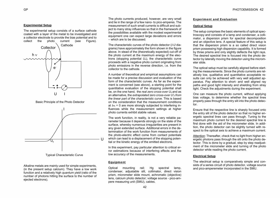
GP PHOTOEMISSION 42

42

Experimental Setup

The experimental setup consists of a surface cathode coated with a layer of the metal to be investigated and a collector electrode to provide the bias potential and to collect the photo current (see Figure).

CollectorCathode

h

e-

U I

Basic Principle of the Photo Detector

I

UU0

Typical Characteristic Curve

Alkaline metals are mainly used for simple experiments, (in the present setup calcium). They have a low work function and a relatively high quantum yield (ratio of the number of photons hitting the surface to the number of ejected electrons).

The photo currents produced, however, are very small and lie in the range of a few nano- to pico-amperes. The measurement of such small currents is difficult and sub-ject to many stray influences so that in the framework of the possibilities available with the modest experimental equipment one can expect large deviations and errors – which are to be discussed.

The characteristic curves of the photo detector (I-U dia-grams) have approximately the form shown in the figure above. In stead of the (theoretically expected) cut-off of the photo current at the maximum energy of the elec-trons (stopping potential Uo), the characteristic curve proceeds with a negative photo current originating from photo emissions in the reverse direction, i.e. from the collector to the cathode.

A number of theoretical and empirical assumptions can be made for a precise discussion and evaluation of the form of the characteristic curves. As far as the experi-ment is concerned (see above), a starting point for the quantitative evaluation of the stopping potential shall be, on the one hand, the real zero cross-over Uo and as an alternative, the extrapolated zero cross-over U'0 from the linear part of the characteristic curve. This is based on the consideration that the measurement conditions at IPh = 0 are more strongly subjected to interfering in-fluences while the measurement settings at higher photo currents exhibit stabile values.

The work function, in reality, is not a very reliable pa-rameter because it depends strongly on the state of the surface, whereby numerous irregularities are present in any given extended surface. Additional errors in the de-termination of the work function from measurements of the photo-electric effect come from contact potentials which can lead to a displacement of the stopping poten-tial or the kinetic energy of the emitted electrons.

In this experiment, pay particular attention to critical er-ror estimations because of interfering effects and the low accuracy of the measurements.

Equipment

Optical mounting rail; Hg spectral lamp, condenser, adjustable slit, collimator, direct vision prism, micrometer slide mount, achromatic (objective) lens, calcium photo detector; voltage source - pico-am-pere measuring unit (SMU), cables.


Optical Setup

The setup comprises the basic elements of optical spec-troscopy and consists of a lamp and condenser, a colli-mator, a dispersion prism for spectral decomposition and an objective lens. A special feature of this setup is that the dispersion prism is a so called direct vision prism possessing high dispersion capability. It is formed by three prisms and only slightly deflects the light rays. The desired spectral line is focused into the photo de-tector by laterally moving the detector using the microm-eter slide.

The optical setup must be carefully aligned before start-ing the measurements. Since the photo currents are rel-atively low, qualitative and quantitative acceptable re-sults can only be achieved with very well adjusted ap-paratus. Pay attention to short- and well aligned ray paths and good light intensity and shielding from stray light. Check the adjustments during the experiment.

One can measure the photo current, without applying bias voltage, to determine whether the spectral lines properly pass through the entry slit into the photo detec-tor.

Ensure that the respective line is sharply focused onto the entry slit of the photo detector so that no higher en-ergetic spectral lines can pass through. Tuning to the maximum photo current for the desired spectral line is first done with the aid of the micrometer slide. In addi-tion, the photo detector can be slightly turned with re-spect to the optical axis to achieve a maximum current.

Attention: Thereafter, check that no light from higher en-ergetic photons pass through the slit onto the photo de-tector. This is done by a gradual, step by step readjust-ment of the micrometer slide and turning of the photo detector while reading the photo current.

Electrical Setup

The electrical setup is comparatively simple and con-sists of a series circuit of photo detector, voltage source and pico-amperemeter incorporated in the SMU.

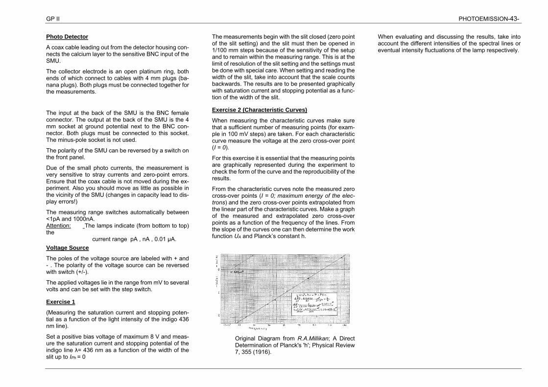
GP II PHOTOEMISSION-43-

Photo Detector

A coax cable leading out from the detector housing con-nects the calcium layer to the sensitive BNC input of the SMU.

The collector electrode is an open platinum ring, both ends of which connect to cables with 4 mm plugs (ba-nana plugs). Both plugs must be connected together for the measurements.

The input at the back of the SMU is the BNC female connector. The output at the back of the SMU is the 4 mm socket at ground potential next to the BNC con-nector. Both plugs must be connected to this socket. The minus-pole socket is not used.

The polarity of the SMU can be reversed by a switch on the front panel.

Due of the small photo currents, the measurement is very sensitive to stray currents and zero-point errors. Ensure that the coax cable is not moved during the ex-periment. Also you should move as little as possible in the vicinity of the SMU (changes in capacity lead to dis-play errors!)

The measuring range switches automatically between <1pA and 1000nA. Attention: The lamps indicate (from bottom to top) the

current range pA , nA , 0.01 μA. Voltage Source

The poles of the voltage source are labeled with + and - . The polarity of the voltage source can be reversed with switch (+/-).

The applied voltages lie in the range from mV to several volts and can be set with the step switch.

Exercise 1

(Measuring the saturation current and stopping poten-tial as a function of the light intensity of the indigo 436 nm line).

Set a positive bias voltage of maximum 8 V and meas-ure the saturation current and stopping potential of the indigo line λ= 436 nm as a function of the width of the slit up to IPh = 0

The measurements begin with the slit closed (zero point of the slit setting) and the slit must then be opened in 1/100 mm steps because of the sensitivity of the setup and to remain within the measuring range. This is at the limit of resolution of the slit setting and the settings must be done with special care. When setting and reading the width of the slit, take into account that the scale counts backwards. The results are to be presented graphically with saturation current and stopping potential as a func-tion of the width of the slit.

Exercise 2 (Characteristic Curves)

When measuring the characteristic curves make sure that a sufficient number of measuring points (for exam-ple in 100 mV steps) are taken. For each characteristic curve measure the voltage at the zero cross-over point (I = 0).

For this exercise it is essential that the measuring points are graphically represented during the experiment to check the form of the curve and the reproducibility of the results.

From the characteristic curves note the measured zero cross-over points (I = 0; maximum energy of the elec-trons) and the zero cross-over points extrapolated from the linear part of the characteristic curves. Make a graph of the measured and extrapolated zero cross-over points as a function of the frequency of the lines. From the slope of the curves one can then determine the work function UA and Planck’s constant h.

Original Diagram from R.A.Millikan; A Direct Determination of Planck's 'h'; Physical Review 7, 355 (1916).

When evaluating and discussing the results, take into account the different intensities of the spectral lines or eventual intensity fluctuations of the lamp respectively.

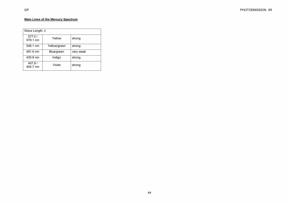
GP PHOTOEMISSION 44

44

Main Lines of the Mercury Spectrum

Wave Length, λ

577.0 / 579.1 nm Yellow strong

546.1 nm Yellow/green strong

491.6 nm Blue/green very weak

435.8 nm Indigo strong

407.8 / 404.7 nm Violet strong

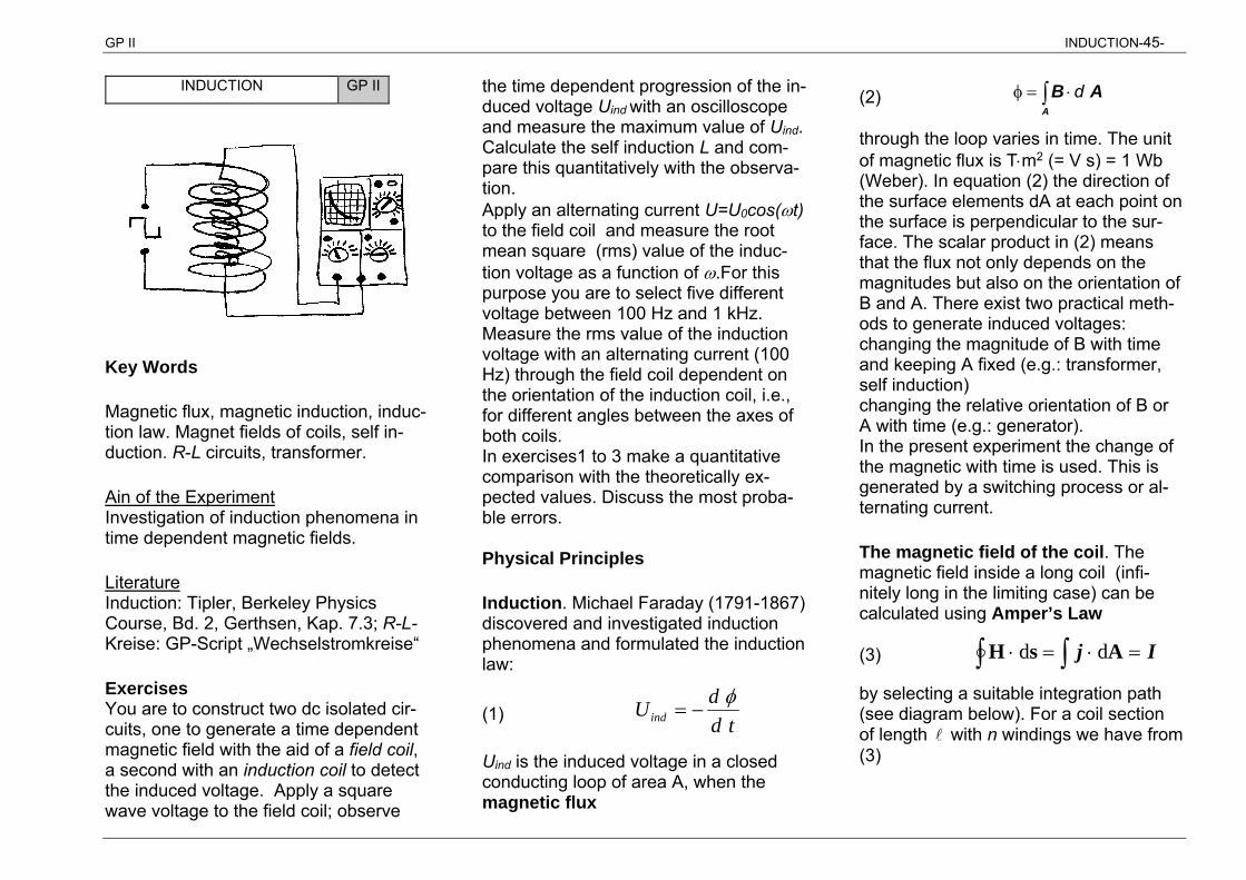
GP II INDUCTION-45-

INDUCTION GP II

Key Words

Magnetic flux, magnetic induction, induc-tion law. Magnet fields of coils, self in-duction. R-L circuits, transformer.

Ain of the Experiment Investigation of induction phenomena in time dependent magnetic fields.

Literature Induction: Tipler, Berkeley Physics Course, Bd. 2, Gerthsen, Kap. 7.3; R-L-Kreise: GP-Script „Wechselstromkreise“

Exercises You are to construct two dc isolated cir-cuits, one to generate a time dependent magnetic field with the aid of a field coil, a second with an induction coil to detect the induced voltage. Apply a square wave voltage to the field coil; observe

the time dependent progression of the in-duced voltage Uind with an oscilloscope and measure the maximum value of Uind. Calculate the self induction L and com-pare this quantitatively with the observa-tion. Apply an alternating current U=U0cos(t) to the field coil and measure the root mean square (rms) value of the induc-tion voltage as a function of .For this purpose you are to select five different voltage between 100 Hz and 1 kHz. Measure the rms value of the induction voltage with an alternating current (100 Hz) through the field coil dependent on the orientation of the induction coil, i.e., for different angles between the axes of both coils. In exercises1 to 3 make a quantitative comparison with the theoretically ex-pected values. Discuss the most proba-ble errors. Physical Principles

Induction. Michael Faraday (1791-1867) discovered and investigated induction phenomena and formulated the induction law:

(1) tddUind

Uind is the induced voltage in a closed conducting loop of area A, when the magnetic flux

(2) A

AB d

through the loop varies in time. The unit of magnetic flux is Tm2 (= V s) = 1 Wb (Weber). In equation (2) the direction of the surface elements dA at each point on the surface is perpendicular to the sur-face. The scalar product in (2) means that the flux not only depends on the magnitudes but also on the orientation of B and A. There exist two practical meth-ods to generate induced voltages: changing the magnitude of B with time and keeping A fixed (e.g.: transformer, self induction) changing the relative orientation of B or A with time (e.g.: generator). In the present experiment the change of the magnetic with time is used. This is generated by a switching process or al-ternating current.

The magnetic field of the coil. The magnetic field inside a long coil (infi-nitely long in the limiting case) can be calculated using Amper’s Law

(3) Ij AsH dd

by selecting a suitable integration path (see diagram below). For a coil section of length with n windings we have from (3)

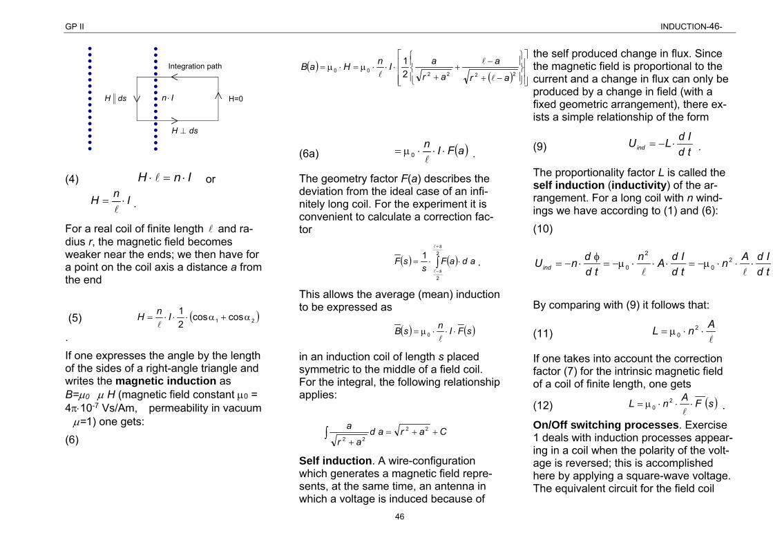
GP II INDUCTION-46-

46

Integration path

dsH

dsH

H=0In

(4) InH or

InH .

For a real coil of finite length and ra-dius r, the magnetic field becomes weaker near the ends; we then have for a point on the coil axis a distance a from the end

(5) 21 coscos21

InH

. If one expresses the angle by the length of the sides of a right-angle triangle and writes the magnetic induction as B=0� H (magnetic field constant 0 = 410-7 Vs/Am,� permeability in vacuum �=1) one gets: (6)

222200 2

1

ar

a

ar

aInHaB

(6a) aFIn

0 .

The geometry factor F(a) describes the deviation from the ideal case of an infi-nitely long coil. For the experiment it is convenient to calculate a correction fac-tor

adaFs

sF

s

s

2

2

1

.

This allows the average (mean) induction to be expressed as

sFInsB 0

in an induction coil of length s placed symmetric to the middle of a field coil. For the integral, the following relationship applies:

Caradar

a

22

22

Self induction. A wire-configuration which generates a magnetic field repre-sents, at the same time, an antenna in which a voltage is induced because of

the self produced change in flux. Since the magnetic field is proportional to the current and a change in flux can only be produced by a change in field (with a fixed geometric arrangement), there ex-ists a simple relationship of the form

(9) tdIdLUind .

The proportionality factor L is called the self induction (inductivity) of the ar-rangement. For a long coil with n wind-ings we have according to (1) and (6): (10)

tdIdAn

tdIdAn

tddnUind

20

2

0

By comparing with (9) it follows that:

(11) AnL 2

0

If one takes into account the correction factor (7) for the intrinsic magnetic field of a coil of finite length, one gets

(12) sFAnL

20 .

On/Off switching processes. Exercise 1 deals with induction processes appear-ing in a coil when the polarity of the volt-age is reversed; this is accomplished here by applying a square-wave voltage. The equivalent circuit for the field coil

GP II INDUCTION-47-

can be taken as a series circuit consist-ing of an ideal coil of inductivity L and a loss resistance RL. The voltage source (function generator) has an open circuit voltage UG and an internal resistance of Ri.

The description of the current in the coil is given by a differential equation after applying Kirchhoff’s rules. The solution, taking into account the boundary condi-tions is (13)

tL

RR

iL

GiL

eRR

UtI 21 .

The switchover point from - UG to + UG was selected as t = 0 and the assump-tion made that the half period of the square-wave voltage is long compared to the decay time.

Induction due to alternating fields. If one generates an alternating magnetic in a field coil by applying a periodic current of the form

(14) tII cos0 ,

the voltage induced in the coil grows pro-portional to the amplitude of the current I0 and to the frequency . Presentation of the Physical Princi-ples

(As part of preparation for the report.) Discussion of the induction law and the relationship between H and B. Solution of the differential equation for the switching process. Notation and discussion of the other equations needed for the measurements. Apparatus and Equipment

Large coil with field windings (1000 wind-ings) and induction windings (125 and 250 windings) on a common body. Exact coil data is found in the lab bench script. Induction coil with adjustable orientation (tilt coil) Function generator Oscilloscope and multimeter.


Operation of the equipment is self-ex-planatory. To Exercise 1: Large coil with field windings n = 1000 and induction windings n = 500. The ter-minals of the windings are located on the front ends of the coil next to each other. The length of the windings is (1901) mm. The field windings are connected directly to the function generator (square-wave function, 100 Hz, amplitude 3 scale divisions).

The oscilloscope is operated in dual mode: at input I the generator terminal voltage = field coil voltage and at input II the voltage in the induction coil is checked. Select the settings at the oscil-loscope as well as the amplitude and fre-quency at the function generator such that the voltage-time curve sufficiently decays. Make optimal use of the screen with respect to resolution and accuracy. Attention: when making sweep- and volt-age settings take note that rotary knobs on the oscilloscope are set to calibrate (cal)! Make a qualitative sketch of the run of the curve in the report book.

With the decay curves UFeld(t) and Uind(t) we are only interested in the voltages with respect to U = U().To compare them with one another and for the quan-titative evaluation of the decay behav-iour, both curves can be placed over each other by suitable settings of the y-deflection at the oscilloscope. Record the data in a table by reading a reasonable number of U(t) values from the cm scale of the screen. For further evaluation, one requires the open-circuit voltage of the generator UG (field coil terminals disconnected) as well as the initial- and final voltage U0 = U(0) and U at the field coil. They are deter-

GP II INDUCTION-48-

48

mined by difference measurements be-tween the positive and negative half-peri-ods to take into account the arbitrary po-sition of the zero point of the generator (dc offset) and the oscilloscope. Carefully measure and record the actual original measurement data (screen read-ings in cm and the associated oscillo-scope settings), since from experience errors easily set in here. The dc re-sistance of the field coil RL is directly measured with a multimeter (METRA Hit 12S). Evaluation is made by plotting the meas-ured voltage-time curve on half-log pa-per. Uind(0) is found by extrapolation of the measured values and L together with RG+RL (see below) from the gradient of the fitted line. The results are to be quali-tatively and quantitatively with the theo-retical expectations. The internal resistance of the function generator RG can be determined from the observed terminal voltage U0 for t = 0 and U for t > with the help of (15):

(15) ,0,0 IRUU GG

(15a) ,0,0)( IRIRRU LLGG

Error Calculations. In the propagation of errors it is advantageous to supple-ment the generator resistance RG in (15) with RL (see 15a) and from this directly calculate "closed" expressions for the re-quired sums of the internal resistances

RG+RL. The relation (15a) is to be evalu-ated for both cases (U0, U).

To Exercise 2: The large coil with n = 1000 field wind-ings and n = 500 induction windings is used. The measurement of the rms values is performed with the multimeter Voltcraft 5050-DB (current measurement) and a milli-voltmeter Grundig MV 40 (voltage measurement). The field current should be about 30 mA. Attention: The field current changes with frequency. (Why?) The frequency de-pendence of the induction voltage Uind(ω) shall be measured in a range from 100 Hz to about 1000 Hz. Plot the results and discuss them quantitatively. Estimate the largest most probable error of the measurement.

To Exercise 3: Large coil n = 1000 as field coil and an additional coil with variable orientation (tilt coil) as the Induction coil. Make measurements of Uind() at 100 Hz. Evaluation is made by plotting Uind against cos . Discuss the results as well as the most probable error sources quantitatively; draw realistic error bars in the plots. Supplementary Questions The following questions are of signifi-cance for the physics of transformers.

How does the induction voltage depend on the frequency when in the field coil the voltage is held constant and not the current? In the oscilloscope observe the the phase between field- and induction volt-age as a function of the frequency. Why are the voltages in-phase at suffi-ciently high frequencies? Connect an ad-dition (low resistance) load to the induc-tion coil. Why does a phase shift now ap-pear even at high frequencies? (Note: consider the energy.)

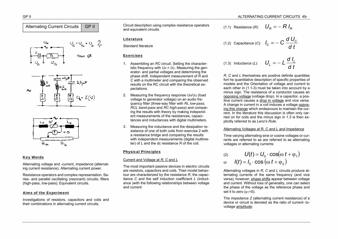
GP II ALTERNATING CURRENT CIRCUITS 49-

Alternating Current Circuits GP II

Key Words

Alternating voltage and -current, impedance (alternat-ing current resistance). Alternating current power.

Resistance operators and complex representation. Se-ries- and parallel oscillating (resonant) circuits; filters (high-pass, low-pass); Equivalent circuits.

Aims of the Experiment

Investigations of resistors, capacitors and coils and their combinations in alternating current circuits.

Circuit description using complex resistance operators and equivalent circuits.

Literature

Standard literature

Exercises

1. Assembling an RC circuit. Setting the character-istic frequency with UR = UC. Measuring the gen-erator- and partial voltages and determining the phase shift. Independent measurement of R and C with a multimeter and comparing the observed results on the RC circuit with the theoretical ex-pectations.

2. Measuring the frequency response UR/UG (load voltage to generator voltage) on an audio fre-quency filter (three-way filter with RL low-pass, RCL band-pass and RC high-pass) and compar-ing the results with theory by making independ-ent measurements of the resistances, capaci-tances and inductances with digital multimeters.

3. Measuring the inductance and the dissipation re-sistance of one of both coils from exercise 2 with a resistance bridge and comparing the results with independent measurements (digital multime-ter) of L and the dc resistance R of the coil.

Physical Principles

Current and Voltage at R, C and L

The most important passive devices in electric circuits are resistors, capacitors and coils. Their model behav-iour are characterized by the resistance R, the capac-itance C and the self induction coefficient L (induct-ance )with the following relationships between voltage and current:

(1.1) Resistance (R): RR IRU

(1.2) Capacitance (C): td

UdCI CC

(1.3) Inductance (L): tdIdLU L

L

R, C and L themselves are positive definite quantities fort he quantitative description of specific properties of models and the Orientation of voltage and current to each other in (1.1-3) must be taken into account by a minus sign. The resistance of a conductor causes an opposing voltage (voltage drop). In a capacitor, a pos-itive current causes a drop in voltage and vice versa. A change in current in a coil induces a voltage oppos-ing this change which endeavours to maintain the cur-rent. In the literature this discussion is often only car-ried on for coils and the minus sign in 1.3 is then ex-plicitly referred to as Lenz’s Rule.

Alternating Voltages at R, C and L and Impedance

Time varying alternating sine or cosine voltages or cur-rents are referred to as are referred to as alternating voltages or alternating currents:

(2) 10 cos)( tUtU

or 20 cos)( tItI

Alternating voltages in R, C and L circuits produce al-ternating currents of the same frequency (and vice versa), however, phase shifts appear between voltage and current. Without loss of generality, one can select the phase of the voltage as the reference phase and set it to zero (1=0).

The impedance Z (alternating current resistance) of a device or circuit is denoted as the ratio of current- to-voltage amplitude:

GP ALTERNATING CURRENT CIRCUITS 50-

50

(3) 0

0

IUZ

Inserting (2) in (1.1-3) gives for the impedance and phase shift of the current to voltage at R, C and L:

(4.1) RZR and

(At the resistor, the phases of voltage and current oppose each other and the prod-uct of voltage times current is always neg-ative corresponding to the sign conven-tion for work or power dissipated. In the literature the sign problem is not always handled consequently, and one also finds the statement that current and voltage at the resistor are "in phase", i.e., equal in phase)

(4.2) C

ZC

1 and 2/

(At the capacitor the “current leads the voltage".)

(4.3) LZL and 2/

(At the coil the "the current trails the volt-age".)

Alternating Current Networks

The impedances and phases of combinations of R, C and L can be calculated analogously to the dc case by using complex resistance operators Z of the devices, whereby, for a

series circuit:

(5.1) iZ Z and

i

i

ZZ

ReIm

tan

and for a parallel circuit:

(5.2) iZ Z

11 and

i

i

Z

Z1Re

1Imtan

GP II ALTERNATING CURRENT CIRCUITS--51-

A detailed presentation of the formalism of ac operators is found in annex IV WECHSELSTROMOPERATOREN of the lab script.

Alternating Current Power

In the complex representation (see WECHSEL-STROMOPERATOREN), the ac power is given by the product of the real parts of U and I.

(6)

**

21

21)Re()Re( IIUUIU P

Setting an alternating voltage and a (phase shifted) al-ternating current for U and I respectively, one obtains for the time averaged power due to the vanishing peri-odic terms

(7)

cosIUcosIUeeIUP rmsrmsii

0000 21

41

where so called root mean square (rms) values were introduced as convenient measurement- and operation quantities, whose products, except for the phase factor, directly reproduce the average power. For alternating voltages and –currents we have according to (7):

(8) 20 /UU rms or

20 /II rms

If in particular R = 0, it follows that = ± /2 and cos = 0, i.e., the ac circuit, on average, does not draw power from the voltage source even though a current flows and voltages build up at C and L. Only R draws power from the circuit in the form of heat dissipation.

Power Losses

At ideal capacitors and coils alone, or at respective combinations with R = 0 or R = , = ± /2 and cos = 0, i.e., the ac power (Urms Irms cos ) is zero averaged

over time, and the ac circuit does not draw power from the voltage source even though a current flows and volt-ages build up at C and L. Only R draws power from the circuit in the form of heat (loss resistance)

In contrast, real capacitors and coils are not loss-less and cannot be described by C and L alone but must be described by an equivalent circuit with additional loss resistance R.

The main reasons for power losses in coils are the re-sistance of the wire, eddy current losses in conducting material close to the coil, and remagnetization losses in coils with iron- or ferrite cores. Losses in capacitors re-sult from the finite conductance of the dielectric and from dielectric losses brought about by a reversal of po-larization, corresponding to remagnetization losses in ferromagnets. Capacitor losses are comparatively small and can be virtually neglected in most cases.

The loss factor d of a coil or capacitor is specified by the reciprocal of the tangent of the phase angle, which de-scribes the ratio of the loss resistance to pure capacitive or inductive resistance:

(9)

tan

1d

Equivalent Circuit Diagrams for real Capacitors and Coils

A real coil exhibits an experimental impedance Z (volt-age-to-current ratio) and a phase angle , which must be reproduced by a model approach. The simplest mod-els are series- or parallel combinations of L and R:

Series equivalent combination (Rs and Ls)

(10.1) 22ss LRZ and

s

s

RL

tan

Parallel equivalent combination (Rp and Lp)

(10.2) 22111

pp LRZ and

p

p

LR

tan

Various loss resistances Rs or Rp, as well as various in-ductances Ls and Lp also belong to the two equivalent circuit diagrams which should reflect the observed physical circumstances (Z, ).Hence we can speak of a certain inductivity of a coil only in connection with a cer-tain equivalent circuit. Even when a series equivalent circuit with coils and a parallel equivalent circuit with ca-pacitors give a basically better view of the situation, both equivalent circuits are effectively the same and can be selected in their application according to the simplest treatment of the problem.

In practice, it may be necessary to take into account the frequency dependency of Z and , which are based on the frequency dependency of the capacitive and induc-tive behaviour of conductor configurations and their losses. Their exact representation can lead to very com-plex equivalent circuits.

Filters (High-pass, Band-pass, Low-pass)

R-C, R-L- and R-C-L devices represent frequency de-pendent voltage dividers (filters) and their frequency re-sponse can be calculated with the help of resistance op-erators. A R-C-L band-pass filter is an oscillating system with an impedance minimum at resonance (series oscil-lating circuit; filter circuit) or an impedance maximum at resonance (parallel oscillating circuit; trap circuit).

Alternating Current (AC) Bridge

An ac bridge corresponds to a Wheatstone bridge and allows comparative measurements of capacitances and inductances (see diagram on the title page).

The balancing condition is, in the case of alternating currents, the agreement of the complex impedances, i.e., the simultaneous agreement of the partial voltages

GP ALTERNATING CURRENT CIRCUITS 50-

52

in both arms of the bridge and the phases (the loss fac-tors of the capacitors or coils being compared must agree).

(11)

b

aL

b

ax

RR

RRR

RR

LL

00

︶and ︵!

Since this is generally not the case, an additional phase balancing resistor R' must be employed to shift the phase of that device with the lowest loss factor (see cir-cuit diagram on the title page; here it is assumed that the coil to be investigated has the lowest loss factor and must be complemented by a phase balancing resistor).

Presentation of the Physical Principles

(as preparation for part of the report): Short summary of the formalism of complex resistance operators for the description of impedance and phase.

Calculation and discussion of the equations needed for the exercises below.


Plug-in circuit board with various circuit elements (coils, capacitors, resistors). 10 turn potentiometer (balancing potentiometer), 10 turn variable resistor (phase balancing resistor) and comparison coil of known inductivity to set-up the bridge. Function generator, multimeter, oscilloscope.


Operation of the measuring instruments and the func-tion generator follows largely from the labelling on the instruments. Please note the additional information in the lab bench script .

To Exercise 1:

Assembling a R-C circuit using a 1 k resistor, a 1 F capacitor and a function generator as driver (see circuit diagram on the title page). Setting the frequency at which the partial voltages at the resistor and capacitor

agree (transfer frequency). Measuring the partial volt-ages and phase shift with the oscilloscope and compar-ing the results with the theoretical expectations.

Attention: With the function generator and the oscillo-scope one input pole of each unit is grounded and the out- and inputs cannot be freely occupied. For one thing, one must ensure that no short to ground occurs. On the other hand, measurement circumstances arise, such as the interchange of poles with respect to a com-mon “sense of rotation”, which must be taken into ac-count when interpreting the results.

To Exercise 2:

Assembling a filter network (frequency filter) corre-sponding to the circuit diagram on the title page. The 8 resistors represent loads (loud speakers). The fre-quency response is determined by measuring the gen-erator voltage and the voltage across the load resistors as a function of frequency in the range 50 Hz to 20 kHz (in suitable gradations of measured values). Take note that the generator voltage does not remain constant be-cause of the comparatively high internal resistance of the function generator (50 ). Evaluation is made by plotting the measured voltage ratios (load/generator) as points against the frequency and fitting the points with a curve to represent the theoretical progression. The val-ues are to be plotted on log-log paper.

To Exercise 3:

Assembling the bridge as shown on the title page.

Lx and Lo are the physical coils used in the circuit, which must be represented by a series circuit of an inductance (Lx,o) and a loss resistance (Rx,o) in the equivalent circuit diagram. A comparator coil Lo of 1.5 mH is available on a plug-in board.

Voltage balancing is made with a 1 k rotary potenti-ometer and phase balancing with a 50 variable resis-tor. Balancing is checked with the multimeter (PHILIPS PM 2505) and performed by successively changing voltage- and phase balancing. In effect, the bridge can only be balanced to a remaining rest voltage since the function generator produces, harmonics (distortions) which cannot be simultaneously balanced in phase.

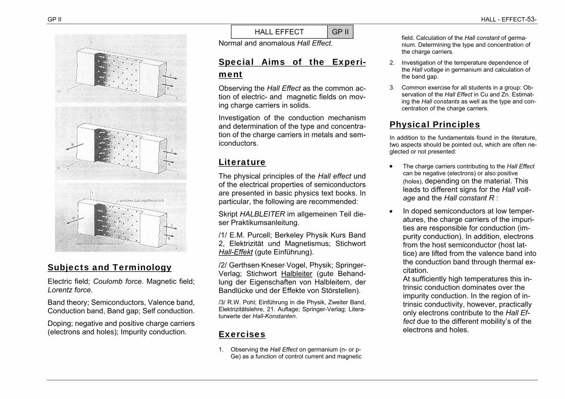
GP II HALL - EFFECT-53-

Subjects and Terminology Electric field; Coulomb force. Magnetic field; Lorentz force.

Band theory; Semiconductors, Valence band, Conduction band, Band gap; Self conduction.

Doping; negative and positive charge carriers (electrons and holes); Impurity conduction.

Normal and anomalous Hall Effect.

Special Aims of the Experi-ment Observing the Hall Effect as the common ac-tion of electric- and magnetic fields on mov-ing charge carriers in solids.

Investigation of the conduction mechanism and determination of the type and concentra-tion of the charge carriers in metals and sem-iconductors.

Literature The physical principles of the Hall effect und of the electrical properties of semiconductors are presented in basic physics text books. In particular, the following are recommended:

Skript HALBLEITER im allgemeinen Teil die-ser Praktikumsanleitung.

/1/ E.M. Purcell; Berkeley Physik Kurs Band 2, Elektrizität und Magnetismus; Stichwort Hall-Effekt (gute Einführung).

/2/ GerthsenKneserVogel, Physik; Springer-Verlag; Stichwort Halbleiter (gute Behand-lung der Eigenschaften von Halbleitern, der Bandlücke und der Effekte von Störstellen). /3/ R.W. Pohl; Einführung in die Physik, Zweiter Band, Elektrizitätslehre, 21. Auflage; Springer-Verlag; Litera-turwerte der Hall-Konstanten.

Exercises 1. Observing the Hall Effect on germanium (n- or p-

Ge) as a function of control current and magnetic

field. Calculation of the Hall constant of germa-nium. Determining the type and concentration of the charge carriers.

2. Investigation of the temperature dependence of the Hall voltage in germanium and calculation of the band gap.

3. Common exercise for all students in a group: Ob-servation of the Hall Effect in Cu and Zn. Estimat-ing the Hall constants as well as the type and con-centration of the charge carriers.

Physical Principles In addition to the fundamentals found in the literature, two aspects should be pointed out, which are often ne-glected or not presented:

The charge carriers contributing to the Hall Effect can be negative (electrons) or also positive (holes), depending on the material. This leads to different signs for the Hall volt-age and the Hall constant R :

In doped semiconductors at low temper-atures, the charge carriers of the impuri-ties are responsible for conduction (im-purity conduction). In addition, electrons from the host semiconductor (host lat-tice) are lifted from the valence band into the conduction band through thermal ex-citation. At sufficiently high temperatures this in-trinsic conduction dominates over the impurity conduction. In the region of in-trinsic conductivity, however, practically only electrons contribute to the Hall Ef-fect due to the different mobility’s of the electrons and holes.

HALL EFFECT GP II

GP HALL EFFECT 54-

54

Presentation of the Physical Principles (as preparation for part of the report): Presen-tation of the Hall Effect and derivation of the Hall voltage. Short statement and discussion of the temperature dependence of the Hall voltage.

Apparatus and Equipment Printed circuit (pc) board with metal probes (n-Ge, p-Ge, Cu and Zn) to determine the Hall Effect and various additional compo-nents for the experimental investigation.

Electromagnet formed by two coils and a U-shaped iron core with pole shoes. Various power supply units. Digital multimeter and a microvolt meter for the measurement of cur-rents and voltages.

Experiment and Evaluation Please handle the pc board with care. Ge crystals are brittle and sensitive to breakage and a fracture of the crystal by bending makes the pc board unusable (cost of a pc board 1000 €). Proceed carefully when placing the pc board in the magnet and con-necting the cables. Compensate the pressure used to plug in and pull out the banana plugs by firmly holding the pc board in the area of the sockets.

Circuitry

The required connections are inscribed on the pc board.

Control Current

The current through the probe is called the control current. In semiconductors it is im-portant to hold the control current constant during the experiment since the resistance is strongly dependent on the temperature.

For this purpose, the pc board incorporates a constant current source which delivers a con-stant current of about 30 mA independent of the external voltage (12 to 30 V). The con-stant current device is connected through outer socket of both (-) sockets for the control current. The constant current device is used to measure the Hall voltage as a function of the magnetic field sine it allows alignment of the resistance-voltage drop (see section on Hall Voltage below).

The constant current device cannot be used to measure the Hall voltage as a function of the control current (inner of both (-) sockets for the control current) and the power supply unit for the control current (Voltcraft) must be used as the constant current device (voltage limiter to maximum and the current adjusted with the current limiter). Proceed with care so that the maximum value of 50 mA for the con-trol current is not exceeded (use the power supply unit with 200 mA limiting current).

With the metal probes, the control current is directly connected with a maximum current of 20 A.

Hall Voltage

The Hall voltage is tapped transverse to the probe dimension. Since both taps for the Hall voltage cannot lie directly opposite each other

due to manufacturing constraints, a re-sistance voltage drop appears in addition to the Hall voltage. To compensate for this the voltage on one side is tapped slightly "above" and "below" the opposite point and aligned with the aid of a potentiometer. This zero-point correction of the Hall voltage is made in each case without applying the magnetic field.

This circuit is only effective in semiconductor probes when the constant current device (see above) is used. When the control current is directly connected to measure the Hall volt-age as a function of the control current, the zero-point must be determined and the meas-ured values accordingly computed.

Heater and Thermocouple

The probe (pc board) is equipped with a heater and thermocouple to investigate the temperature dependence of the Hall voltage.

Magnet

When connecting the magnet, pay attention to the correct series connection of the coils. A power supply unit (Voltcraft 0...30 V, 2 A) de-livers the current for the magnet.

The lab bench script contains a calibration curve for the magnetic field in the center of the pole shoes as a function of magnetic cur-rent; the magnetic current must not exceed 2 A .

Attention: To check the polarity of Hall volt-age with respect to the sign of the charge car-riers one must very carefully take into account and document the orientation of all experi-mental quantities (magnetic field from the

GP II HALL - EFFECT-55-

sense of the windings of the coil and the di-rection of the magnetic current, direction of the control current or polarity of the connec-tion of the control current source, polarity of the Hall voltage or polarity of the connection of the voltage measuring instrument). A sketch of the experimental set-up is essential to clearly show the orientations and connec-tions of the measuring instruments! When re-cording the values of the Hall voltage the sign must always be given!

To Exercise 1:

A second Voltcraft power supply unit ("200-mA" unit) is used as the control current source.

To investigate the Hall voltage as a function of the magnetic field one uses the constant current source on the pc board (outer (-) sock-ets) and the potentiometer (rotating pin) to align the resistance-voltage drop.

For the measurement as a function of the control current, the inner "direct" sockets must be connected; see the general infor-mation concerning the Hall voltage above.

The control current must not exceed 50 mA.

The alignment potentiometer for the re-sistance-voltage drop is inhibited when the constant current source is not connected, and to correct the voltage values, the voltage drop for each control current value must be meas-ured with the magnetic field switched off (switch off the magnetic current power supply at the mains switch) and the measured value computed with the correction.

The control current and the Hall voltage are measured with two digital multimeters.

To Exercise 2:

In addition to the circuitry for exercise 1, the heating current source and a further multime-ter is connected to measure the thermo-volt-age and the Hall voltage as a function of tem-perature.

The heater is operated with 6 V ac and the heating current is then about 5 A. The tem-perature coefficient of the thermocouple is 40 V/K (temperature difference to room temper-ature).

The temperature of the pc board must not exceed 150 °C corresponding to 5 mV thermo-voltage!

The heater (step transformer) should be used intermittently (momentary switch-on with pauses) so that the rate of heating is not too fast in order to ensure safe control and relia-ble recordings of the measured values.

The thermo-voltage can (still) be measured with the digital multimeters. The measuring accuracy is clearly limited by the low resolu-tion (0.1 mV corresponding to 2.5 K) but may be considered as sufficient within the scope of the other measurement conditions (e.g., temperature gradients) and the aims of the experiment.

With a suitable logarithmic plot (see equation 1 in annex V „HALBLEITER“ in the lab script ) the Hall voltage shows, in the high tempera-ture range (intrinsic conduction), the ex-pected linear progression from which one can determine the band gap E .

To Exercise 3

A 10 A power supply unit is available to meas-ure the Hall Effect on metal probes (copper and zinc) which require high control currents. The Hall voltage, however, remains compar-atively small and must be measured with a sensitive microvolt meter (KNICK) or for com-parison purposes with the digital multimeter (HP 3457A).

The measurements on the metal probes have only qualitative character with respect to the sign because of experimental difficulties (foils with large tolerances as thin probes; how-ever, very small values for the Hall voltage). Since only one power supply unit for the high currents and one microvolt meter are availa-ble, the measurements shall be made as a common exercise for the whole group but re-ported and evaluated for each pair of students working together.

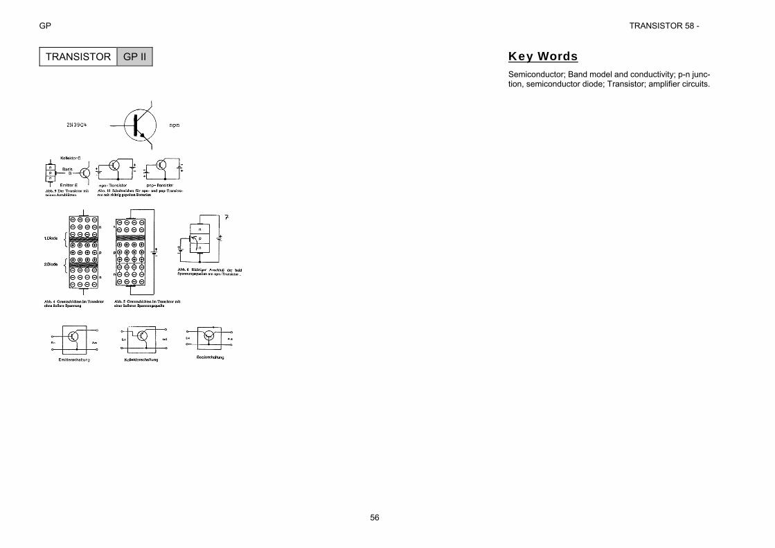
GP TRANSISTOR 58 -

56

TRANSISTOR GP II

Key Words Semiconductor; Band model and conductivity; p-n junc-tion, semiconductor diode; Transistor; amplifier circuits.

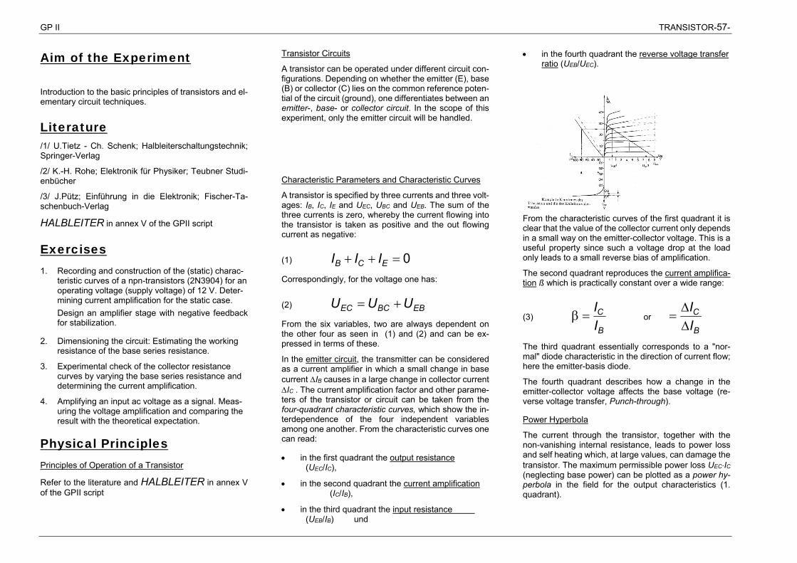
GP II TRANSISTOR-57-


Introduction to the basic principles of transistors and el-ementary circuit techniques.

Literature /1/ U.Tietz - Ch. Schenk; Halbleiterschaltungstechnik; Springer-Verlag

/2/ K.-H. Rohe; Elektronik für Physiker; Teubner Studi-enbücher

/3/ J.Pütz; Einführung in die Elektronik; Fischer-Ta-schenbuch-Verlag

HALBLEITER in annex V of the GPII script

Exercises 1. Recording and construction of the (static) charac-

teristic curves of a npn-transistors (2N3904) for an operating voltage (supply voltage) of 12 V. Deter-mining current amplification for the static case. Design an amplifier stage with negative feedback for stabilization.

2. Dimensioning the circuit: Estimating the working resistance of the base series resistance.

3. Experimental check of the collector resistance curves by varying the base series resistance and determining the current amplification.

4. Amplifying an input ac voltage as a signal. Meas-uring the voltage amplification and comparing the result with the theoretical expectation.

Physical Principles Principles of Operation of a Transistor

Refer to the literature and HALBLEITER in annex V of the GPII script

Transistor Circuits

A transistor can be operated under different circuit con-figurations. Depending on whether the emitter (E), base (B) or collector (C) lies on the common reference poten-tial of the circuit (ground), one differentiates between an emitter-, base- or collector circuit. In the scope of this experiment, only the emitter circuit will be handled.

Characteristic Parameters and Characteristic Curves

A transistor is specified by three currents and three volt-ages: IB, IC, IE and UEC, UBC and UEB. The sum of the three currents is zero, whereby the current flowing into the transistor is taken as positive and the out flowing current as negative:

(1) 0 ECB III

Correspondingly, for the voltage one has:

(2) EBBCEC UUU

From the six variables, two are always dependent on the other four as seen in (1) and (2) and can be ex-pressed in terms of these.

In the emitter circuit, the transmitter can be considered as a current amplifier in which a small change in base current IB causes in a large change in collector current IC . The current amplification factor and other parame-ters of the transistor or circuit can be taken from the four-quadrant characteristic curves, which show the in-terdependence of the four independent variables among one another. From the characteristic curves one can read:

in the first quadrant the output resistance (UEC/IC),

in the second quadrant the current amplification (IC/IB),

in the third quadrant the input resistance (UEB/IB) und

in the fourth quadrant the reverse voltage transfer ratio (UEB/UEC).

From the characteristic curves of the first quadrant it is clear that the value of the collector current only depends in a small way on the emitter-collector voltage. This is a useful property since such a voltage drop at the load only leads to a small reverse bias of amplification.

The second quadrant reproduces the current amplifica-tion ß which is practically constant over a wide range:

(3) B

C

II

or B

C

II

The third quadrant essentially corresponds to a "nor-mal" diode characteristic in the direction of current flow; here the emitter-basis diode.

The fourth quadrant describes how a change in the emitter-collector voltage affects the base voltage (re-verse voltage transfer, Punch-through).

Power Hyperbola

The current through the transistor, together with the non-vanishing internal resistance, leads to power loss and self heating which, at large values, can damage the transistor. The maximum permissible power loss UECIC (neglecting base power) can be plotted as a power hy-perbola in the field for the output characteristics (1. quadrant).

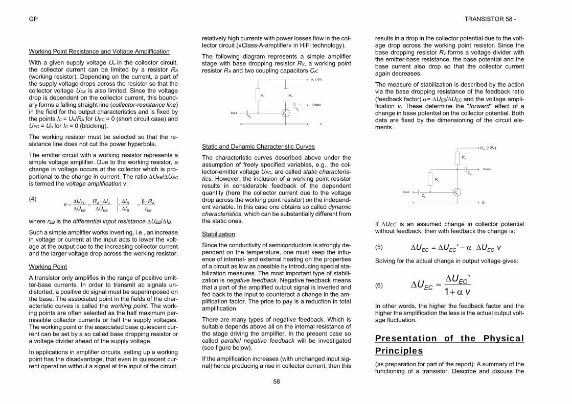
GP TRANSISTOR 58 -

58

Working Point Resistance and Voltage Amplification

With a given supply voltage Uo in the collector circuit, the collector current can be limited by a resistor RA (working resistor). Depending on the current, a part of the supply voltage drops across the resistor so that the collector voltage UCE is also limited. Since the voltage drop is dependent on the collector current, this bound-ary forms a falling straight line (collector-resistance line) in the field for the output characteristics and is fixed by the points IC = Uo/RA for UEC = 0 (short circuit case) and UEC = Uo for IC = 0 (blocking).

The working resistor must be selected so that the re-sistance line does not cut the power hyperbola.

The emitter circuit with a working resistor represents a simple voltage amplifier. Due to the working resistor, a change in voltage occurs at the collector which is pro-portional to the change in current. The ratio UEB/UEC is termed the voltage amplification v:

(4)

EB

A

B

B

EB

CA

EB

EC

rR

II

UIR

UUv

where rEB is the differential input resistance UEB/IB.

Such a simple amplifier works inverting, i.e., an increase in voltage or current at the input acts to lower the volt-age at the output due to the increasing collector current and the larger voltage drop across the working resistor.

Working Point

A transistor only amplifies in the range of positive emit-ter-base currents. In order to transmit ac signals un-distorted, a positive dc signal must be superimposed on the base. The associated point in the fields of the char-acteristic curves is called the working point. The work-ing points are often selected as the half maximum per-missible collector currents or half the supply voltages. The working point or the associated base quiescent cur-rent can be set by a so called base dropping resistor or a voltage divider ahead of the supply voltage.

In applications in amplifier circuits, setting up a working point has the disadvantage, that even in quiescent cur-rent operation without a signal at the input of the circuit,

relatively high currents with power losses flow in the col-lector circuit (»Class-A-amplifier« in HiFi technology).

The following diagram represents a simple amplifier stage with base dropping resistor RV, a working point resistor RA and two coupling capacitors CK:

U0 (12V)

Output

0

Ck

RARV

Ck

Input

Static and Dynamic Characteristic Curves

The characteristic curves described above under the assumption of freely specified variables, e.g., the col-lector-emitter voltage UEC, are called static characteris-tics. However, the inclusion of a working point resistor results in considerable feedback of the dependent quantity (here the collector current due to the voltage drop across the working point resistor) on the independ-ent variable. In this case one obtains so called dynamic characteristics, which can be substantially different from the static ones.

Stabilization

Since the conductivity of semiconductors is strongly de-pendent on the temperature, one must keep the influ-ence of internal- and external heating on the properties of a circuit as low as possible by introducing special sta-bilization measures. The most important type of stabili-zation is negative feedback. Negative feedback means that a part of the amplified output signal is inverted and fed back to the input to counteract a change in the am-plification factor. The price to pay is a reduction in total amplification.

There are many types of negative feedback. Which is suitable depends above all on the internal resistance of the stage driving the amplifier. In the present case so called parallel negative feedback will be investigated (see figure below).

If the amplification increases (with unchanged input sig-nal) hence producing a rise in collector current, then this

results in a drop in the collector potential due to the volt-age drop across the working point resistor. Since the base dropping resistor Rv forms a voltage divider with the emitter-base resistance, the base potential and the base current also drop so that the collector current again decreases.

The measure of stabilization is described by the action via the base dropping resistance of the feedback ratio (feedback factor) = UEB/UEC and the voltage ampli-fication v. These determine the "forward" effect of a change in base potential on the collector potential. Both data are fixed by the dimensioning of the circuit ele-ments.

U0 (12V)

0

Ck

Ck

Input

Output

RV

RA

If UEC' is an assumed change in collector potential without feedback, then with feedback the change is:

(5) vUUU ECECEC '

Solving for the actual change in output voltage gives:

(6) v

UU ECEC

1'

In other words, the higher the feedback factor and the higher the amplification the less is the actual output volt-age fluctuation.

Presentation of the Physical Principles (as preparation for part of the report): A summary of the functioning of a transistor. Describe and discuss the

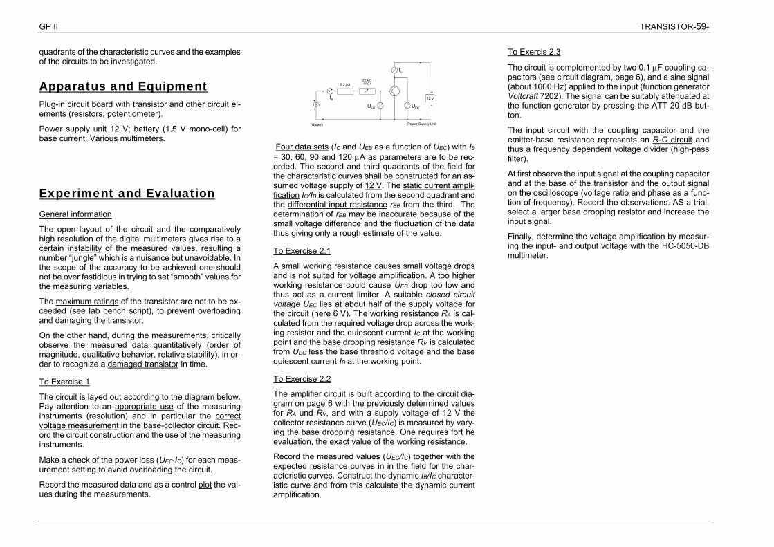
GP II TRANSISTOR-59-

quadrants of the characteristic curves and the examples of the circuits to be investigated.

Apparatus and Equipment Plug-in circuit board with transistor and other circuit el-ements (resistors, potentiometer).

Power supply unit 12 V; battery (1.5 V mono-cell) for base current. Various multimeters.

Experiment and Evaluation General information

The open layout of the circuit and the comparatively high resolution of the digital multimeters gives rise to a certain instability of the measured values, resulting a number “jungle” which is a nuisance but unavoidable. In the scope of the accuracy to be achieved one should not be over fastidious in trying to set “smooth” values for the measuring variables.

The maximum ratings of the transistor are not to be ex-ceeded (see lab bench script), to prevent overloading and damaging the transistor.

On the other hand, during the measurements, critically observe the measured data quantitatively (order of magnitude, qualitative behavior, relative stability), in or-der to recognize a damaged transistor in time.

To Exercise 1

The circuit is layed out according to the diagram below. Pay attention to an appropriate use of the measuring instruments (resolution) and in particular the correct voltage measurement in the base-collector circuit. Rec-ord the circuit construction and the use of the measuring instruments.

Make a check of the power loss (UECIC) for each meas-urement setting to avoid overloading the circuit.

Record the measured data and as a control plot the val-ues during the measurements.

Battery Power Supply Unit

1,5 V+

-

2.2 k22 klog

12 V

+

-

IC

UECUEB

IB

Four data sets (IC and UEB as a function of UEC) with IB = 30, 60, 90 and 120 A as parameters are to be rec-orded. The second and third quadrants of the field for the characteristic curves shall be constructed for an as-sumed voltage supply of 12 V. The static current ampli-fication IC/IB is calculated from the second quadrant and the differential input resistance rEB from the third. The determination of rEB may be inaccurate because of the small voltage difference and the fluctuation of the data thus giving only a rough estimate of the value.

To Exercise 2.1

A small working resistance causes small voltage drops and is not suited for voltage amplification. A too higher working resistance could cause UEC drop too low and thus act as a current limiter. A suitable closed circuit voltage UEC lies at about half of the supply voltage for the circuit (here 6 V). The working resistance RA is cal-culated from the required voltage drop across the work-ing resistor and the quiescent current IC at the working point and the base dropping resistance RV is calculated from UEC less the base threshold voltage and the base quiescent current IB at the working point.

To Exercise 2.2

The amplifier circuit is built according to the circuit dia-gram on page 6 with the previously determined values for RA und RV, and with a supply voltage of 12 V the collector resistance curve (UEC/IC) is measured by vary-ing the base dropping resistance. One requires fort he evaluation, the exact value of the working resistance.

Record the measured values (UEC/IC) together with the expected resistance curves in in the field for the char-acteristic curves. Construct the dynamic IB/IC character-istic curve and from this calculate the dynamic current amplification.

To Exercis 2.3

The circuit is complemented by two 0.1 F coupling ca-pacitors (see circuit diagram, page 6), and a sine signal (about 1000 Hz) applied to the input (function generator Voltcraft 7202). The signal can be suitably attenuated at the function generator by pressing the ATT 20-dB but-ton.

The input circuit with the coupling capacitor and the emitter-base resistance represents an R-C circuit and thus a frequency dependent voltage divider (high-pass filter).

At first observe the input signal at the coupling capacitor and at the base of the transistor and the output signal on the oscilloscope (voltage ratio and phase as a func-tion of frequency). Record the observations. AS a trial, select a larger base dropping resistor and increase the input signal.

Finally, determine the voltage amplification by measur-ing the input- and output voltage with the HC-5050-DB multimeter.

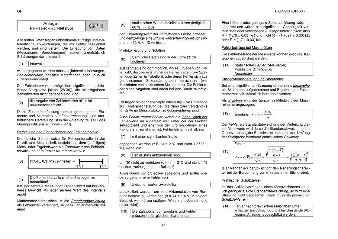
GP TRANSISTOR 58 -

60

Anlage I FEHLERRECHNUNG GP II

Alle realen Daten tragen unbestimmte zufällige und sys-tematische Abweichungen, die als Fehler bezeichnet werden, und sind verteilt. Die Erhebung von Daten (Messungen, Berechnungen) stellen grundsätzlich Schätzungen dar, die durch

(1) Intervalle

wiedergegeben werden müssen (Intervallschätzungen, Fehlerintervalle; inhaltlich zutreffender, aber unüblich Ergebnisintervalle)!

Die Fehlerintervalle ermöglichen signifikante, schlie-ßende Vergleiche [siehe (28-30)], die mit singulären Zahlenwerten nicht gegeben sind, und

(2) die Angabe von Zahlenwerten allein ist unwissenschaftlich!

Diese Zusammenfassung enthält grundlegende Ele-mente und Methoden der Fehlerrechnung; eine aus-führlichere Darstellung ist in der Anleitung zu Teil I des Grundpraktikums zu finden (GP I).

Darstellung und Eigenschaften der Fehlerintervalle

Die übliche Schreibweise für Fehlerintervalle in der Physik und Messtechnik besteht aus dem (zufälligen) Mess- oder Ergebniswert als Zentralwert des Fehlerin-tervalls und dem Fehler als Intervallradius:

(3) (17,4 0,3) Maßeinheiten =

17,1 17,7

(4) Die Fehlerintervalle sind als homogen zu betrachten!

d.h. der zentrale Mess- oder Ergebniswert hat kein hö-heres Gewicht als jeder andere Wert des Intervalls auch!

Mathematisch-statistisch ist die Standardabweichung als Fehlermaß vereinbart, so dass Fehlerintervalle mit einer

(5) statistischen Wahrscheinlichkeit von (lediglich) 68 % ( 2/3)

den Erwartungswert der betreffenden Größe erfassen, und demzufolge eine Irrtumswahrscheinlichkeit von (im-merhin) 32 % 1/3 verbleibt.

Protokollierung und Notation

(6) Sämtliche Daten sind in der Form (3) zu notieren!

Ausnahmen sind dort möglich, wo es Gruppen von Da-ten gibt, die übereinstimmende Fehler tragen (wie Spal-ten oder Zeilen in Tabellen), oder deren Fehler sich aus gemeinsamen Sekundärangaben berechnen (wie Messdaten von elektrischen Multimetern). Die Fehler o-der diese Angaben sind direkt bei den Daten zu notie-ren.

Oft tragen situationsbedingte oder subjektive Umstände zur Fehlerabschätzung bei, die dann zum Verständnis für Dritte im Messprotokoll zu dokumentieren sind.

Auch Fehler tragen Fehler, wobei die Genauigkeit der Fehlerwerte im allgemein weit unter der der Größen selbst bleibt und eher von der Größenordnung eines Faktors 2 anzunehmen ist. Fehler dürfen deshalb nur

(7) mit einer signifikanten Stelle

angegeben werden (z.B. I = 2 % und nicht 1,3725... %), wobei die

(8) Fehler stets aufzurunden sind,

um (5) nicht zu verletzen (d.h. I = 2 % und nicht 1 % bei dem vorhergehenden Beispiel)!

Abweichend von (7) sollen abgelegte und später wie-deraufgenommene Fehler von

(9) Zwischenwerten zweistellig

protokolliert werden, um eine Akkumulation von Run-dungsfehlern zu vermeiden (d.h. I = 1,4 % in obigem Beispiel, wenn I zur späteren Widerstandsberechnung notiert wird).

(10) Die Zahlwörter von Ergebnis und Fehler müssen in der gleichen Stelle enden!

Eine höhere oder geringere Zahlenauflösung wäre in-kohärent und würde nichtsignifikante Genauigkeit vor-täuschen oder vorhandene Aussage unterdrücken; also R = (1,70 0,03) k und nicht R = (1,7027 0,03) k oder R = (1,7 0,03) k.

Fehlerbeiträge bei Messgrößen

Die Fehlerbeiträge der Messwerte können grob drei Ka-tegorien zugeordnet werden:

(11) Statistischer Fehler (Streufehler) Praktische Schätzfehler Nennfehler

Stichprobenschätzung und Streufehler

Bei einer signifikanten Streuung können eine Messreihe als Stichprobe aufgenommen und Ergebnis und Fehler mathematisch-statistisch berechnet werden.

Als Ergebnis wird der (einzelne) Mittelwert der Mess-reihe herangezogen:

(12) Ergebnis nx

xx i

Der Fehler als Standardabweichung der Verteilung die-ser Mittelwerte wird durch die Standardabweichung der Grundverteilung der Einzelwerte und durch den Umfang der Stichprobe bestimmt (statistisches Gewicht):

(13)

Fehler

1

1)()(2

2

nnxx

nn

xx

nxxx i

i

(Der Nenner n-1 berücksichtigt den Näherungscharak-ter bei der Berechnung von (x) aus einer Stichprobe).

Praktischer Schätzfehler

Ist das Auflösevermögen eines Messverfahrens deut-lich geringer als die Standardabweichung, so wird eine Streuung nicht beobachtet. Dann muss als praktischer Schätzfehler ein

(14) Fehler nach praktischen Maßgaben unter kritischer Berücksichtigung aller Umstände (Ab-lesung, Anzeige) abgeschätzt werden.

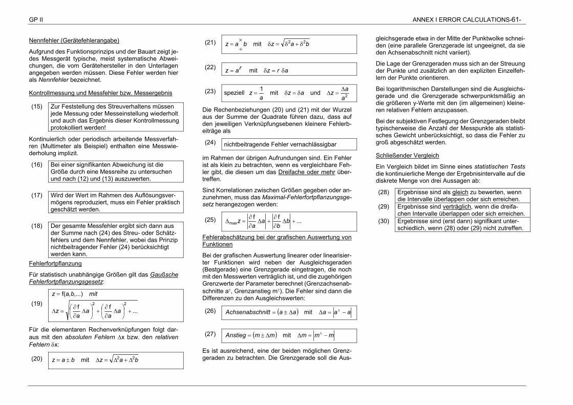
GP II ANNEX I ERROR CALCULATIONS-61-

Nennfehler (Gerätefehlerangabe)

Aufgrund des Funktionsprinzips und der Bauart zeigt je-des Messgerät typische, meist systematische Abwei-chungen, die vom Gerätehersteller in den Unterlagen angegeben werden müssen. Diese Fehler werden hier als Nennfehler bezeichnet.

Kontrollmessung und Messfehler bzw. Messergebnis

(15) Zur Feststellung des Streuverhaltens müssen jede Messung oder Messeinstellung wiederholt und auch das Ergebnis dieser Kontrollmessung protokolliert werden!

Kontinuierlich oder periodisch arbeitende Messverfah-ren (Multimeter als Beispiel) enthalten eine Messwie-derholung implizit.

(16) Bei einer signifikanten Abweichung ist die Größe durch eine Messreihe zu untersuchen und nach (12) und (13) auszuwerten.

(17) Wird der Wert im Rahmen des Auflösungsver-mögens reproduziert, muss ein Fehler praktisch geschätzt werden.

(18) Der gesamte Messfehler ergibt sich dann aus der Summe nach (24) des Streu- oder Schätz-fehlers und dem Nennfehler, wobei das Prinzip nichtbeitragender Fehler (24) berücksichtigt werden kann.

Fehlerfortpflanzung

Für statistisch unabhängige Größen gilt das Gaußsche Fehlerfortpflanzungsgesetz:

(19) ...ff

,...),f(22

aa

aa

z

mitbaz

Für die elementaren Rechenverknüpfungen folgt dar-aus mit den absoluten Fehlern x bzw. den relativen Fehlern x:

(20) bazbaz 22mit

(21) bazbaz 22mit

(22) arzraz mit

(23) speziell 2undmit1a

azaza

z

Die Rechenbeziehungen (20) und (21) mit der Wurzel aus der Summe der Quadrate führen dazu, dass auf den jeweiligen Verknüpfungsebenen kleinere Fehlerb-eiträge als

(24) nichtbeitragende Fehler vernachlässigbar

im Rahmen der übrigen Aufrundungen sind. Ein Fehler ist als klein zu betrachten, wenn es vergleichbare Feh-ler gibt, die diesen um das Dreifache oder mehr über-treffen.

Sind Korrelationen zwischen Größen gegeben oder an-zunehmen, muss das Maximal-Fehlerfortpflanzungsge-setz herangezogen werden:

(25) ...ffmax

bb

aa

z

Fehlerabschätzung bei der grafischen Auswertung von Funktionen

Bei der grafischen Auswertung linearer oder linearisier-ter Funktionen wird neben der Ausgleichsgeraden (Bestgerade) eine Grenzgerade eingetragen, die noch mit den Messwerten verträglich ist, und die zugehörigen Grenzwerte der Parameter berechnet (Grenzachsenab-schnitte a, Grenzanstieg m). Die Fehler sind dann die Differenzen zu den Ausgleichswerten:

(26) aaaaahnittAchsenabsc mit

(27) mmmmmAnstieg mit

Es ist ausreichend, eine der beiden möglichen Grenz-geraden zu betrachten. Die Grenzgerade soll die Aus-

gleichsgerade etwa in der Mitte der Punktwolke schnei-den (eine parallele Grenzgerade ist ungeeignet, da sie den Achsenabschnitt nicht variiert).

Die Lage der Grenzgeraden muss sich an der Streuung der Punkte und zusätzlich an den expliziten Einzelfeh-lern der Punkte orientieren.

Bei logarithmischen Darstellungen sind die Ausgleichs-gerade und die Grenzgerade schwerpunktsmäßig an die größeren y-Werte mit den (im allgemeinen) kleine-ren relativen Fehlern anzupassen.

Bei der subjektiven Festlegung der Grenzgeraden bleibt typischerweise die Anzahl der Messpunkte als statisti-sches Gewicht unberücksichtigt, so dass die Fehler zu groß abgeschätzt werden.

Schließender Vergleich

Ein Vergleich bildet im Sinne eines statistischen Tests die kontinuierliche Menge der Ergebnisintervalle auf die diskrete Menge von drei Aussagen ab:

(28) Ergebnisse sind als gleich zu bewerten, wenn die Intervalle überlappen oder sich erreichen.

(29) Ergebnisse sind verträglich, wenn die dreifa-chen Intervalle überlappen oder sich erreichen.

(30) Ergebnisse sind (erst dann) signifikant unter-schiedlich, wenn (28) oder (29) nicht zutreffen.

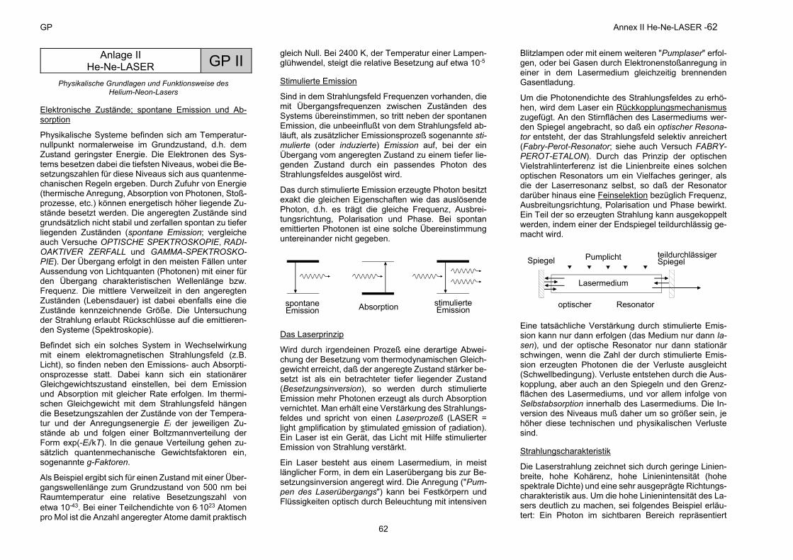
GP Annex II He-Ne-LASER -62

62

Anlage II He-Ne-LASER GP II

Physikalische Grundlagen und Funktionsweise des Helium-Neon-Lasers

Elektronische Zustände; spontane Emission und Ab-sorption

Physikalische Systeme befinden sich am Temperatur-nullpunkt normalerweise im Grundzustand, d.h. dem Zustand geringster Energie. Die Elektronen des Sys-tems besetzen dabei die tiefsten Niveaus, wobei die Be-setzungszahlen für diese Niveaus sich aus quantenme-chanischen Regeln ergeben. Durch Zufuhr von Energie (thermische Anregung, Absorption von Photonen, Stoß-prozesse, etc.) können energetisch höher liegende Zu-stände besetzt werden. Die angeregten Zustände sind grundsätzlich nicht stabil und zerfallen spontan zu tiefer liegenden Zuständen (spontane Emission; vergleiche auch Versuche OPTISCHE SPEKTROSKOPIE, RADI-OAKTIVER ZERFALL und GAMMA-SPEKTROSKO-PIE). Der Übergang erfolgt in den meisten Fällen unter Aussendung von Lichtquanten (Photonen) mit einer für den Übergang charakteristischen Wellenlänge bzw. Frequenz. Die mittlere Verweilzeit in den angeregten Zuständen (Lebensdauer) ist dabei ebenfalls eine die Zustände kennzeichnende Größe. Die Untersuchung der Strahlung erlaubt Rückschlüsse auf die emittieren-den Systeme (Spektroskopie).

Befindet sich ein solches System in Wechselwirkung mit einem elektromagnetischen Strahlungsfeld (z.B. Licht), so finden neben den Emissions- auch Absorpti-onsprozesse statt. Dabei kann sich ein stationärer Gleichgewichtszustand einstellen, bei dem Emission und Absorption mit gleicher Rate erfolgen. Im thermi-schen Gleichgewicht mit dem Strahlungsfeld hängen die Besetzungszahlen der Zustände von der Tempera-tur und der Anregungsenergie Ei der jeweiligen Zu-stände ab und folgen einer Boltzmannverteilung der Form exp(-Ei/kT). In die genaue Verteilung gehen zu-sätzlich quantenmechanische Gewichtsfaktoren ein, sogenannte g-Faktoren.

Als Beispiel ergibt sich für einen Zustand mit einer Über-gangswellenlänge zum Grundzustand von 500 nm bei Raumtemperatur eine relative Besetzungszahl von etwa 10-43. Bei einer Teilchendichte von 61023 Atomen pro Mol ist die Anzahl angeregter Atome damit praktisch

gleich Null. Bei 2400 K, der Temperatur einer Lampen-glühwendel, steigt die relative Besetzung auf etwa 10-5

Stimulierte Emission

Sind in dem Strahlungsfeld Frequenzen vorhanden, die mit Übergangsfrequenzen zwischen Zuständen des Systems übereinstimmen, so tritt neben der spontanen Emission, die unbeeinflußt von dem Strahlungsfeld ab-läuft, als zusätzlicher Emissionsprozeß sogenannte sti-mulierte (oder induzierte) Emission auf, bei der ein Übergang vom angeregten Zustand zu einem tiefer lie-genden Zustand durch ein passendes Photon des Strahlungsfeldes ausgelöst wird.

Das durch stimulierte Emission erzeugte Photon besitzt exakt die gleichen Eigenschaften wie das auslösende Photon, d.h. es trägt die gleiche Frequenz, Ausbrei-tungsrichtung, Polarisation und Phase. Bei spontan emittierten Photonen ist eine solche Übereinstimmung untereinander nicht gegeben.

spontaneEmission Absorption stimulierte

Emission

Das Laserprinzip

Wird durch irgendeinen Prozeß eine derartige Abwei-chung der Besetzung vom thermodynamischen Gleich-gewicht erreicht, daß der angeregte Zustand stärker be-setzt ist als ein betrachteter tiefer liegender Zustand (Besetzungsinversion), so werden durch stimulierte Emission mehr Photonen erzeugt als durch Absorption vernichtet. Man erhält eine Verstärkung des Strahlungs-feldes und spricht von einen Laserprozeß (LASER = light amplification by stimulated emission of radiation). Ein Laser ist ein Gerät, das Licht mit Hilfe stimulierter Emission von Strahlung verstärkt.

Ein Laser besteht aus einem Lasermedium, in meist länglicher Form, in dem ein Laserübergang bis zur Be-setzungsinversion angeregt wird. Die Anregung ("Pum-pen des Laserübergangs") kann bei Festkörpern und Flüssigkeiten optisch durch Beleuchtung mit intensiven

Blitzlampen oder mit einem weiteren "Pumplaser" erfol-gen, oder bei Gasen durch Elektronenstoßanregung in einer in dem Lasermedium gleichzeitig brennenden Gasentladung.

Um die Photonendichte des Strahlungsfeldes zu erhö-hen, wird dem Laser ein Rückkopplungsmechanismus zugefügt. An den Stirnflächen des Lasermediums wer-den Spiegel angebracht, so daß ein optischer Resona-tor entsteht, der das Strahlungsfeld selektiv anreichert (Fabry-Perot-Resonator; siehe auch Versuch FABRY-PEROT-ETALON). Durch das Prinzip der optischen Vielstrahlinterferenz ist die Linienbreite eines solchen optischen Resonators um ein Vielfaches geringer, als die der Laserresonanz selbst, so daß der Resonator darüber hinaus eine Feinselektion bezüglich Frequenz, Ausbreitungsrichtung, Polarisation und Phase bewirkt. Ein Teil der so erzeugten Strahlung kann ausgekoppelt werden, indem einer der Endspiegel teildurchlässig ge-macht wird.

Pumplicht

Lasermedium

teildurchlässiger Spiegel

optischer Resonator

Spiegel

Eine tatsächliche Verstärkung durch stimulierte Emis-sion kann nur dann erfolgen (das Medium nur dann la-sen), und der optische Resonator nur dann stationär schwingen, wenn die Zahl der durch stimulierte Emis-sion erzeugten Photonen die der Verluste ausgleicht (Schwellbedingung). Verluste entstehen durch die Aus-kopplung, aber auch an den Spiegeln und den Grenz-flächen des Lasermediums, und vor allem infolge von Selbstabsorption innerhalb des Lasermediums. Die In-version des Niveaus muß daher um so größer sein, je höher diese technischen und physikalischen Verluste sind.

Strahlungscharakteristik

Die Laserstrahlung zeichnet sich durch geringe Linien-breite, hohe Kohärenz, hohe Linienintensität (hohe spektrale Dichte) und eine sehr ausgeprägte Richtungs-charakteristik aus. Um die hohe Linienintensität des La-sers deutlich zu machen, sei folgendes Beispiel erläu-tert: Ein Photon im sichtbaren Bereich repräsentiert

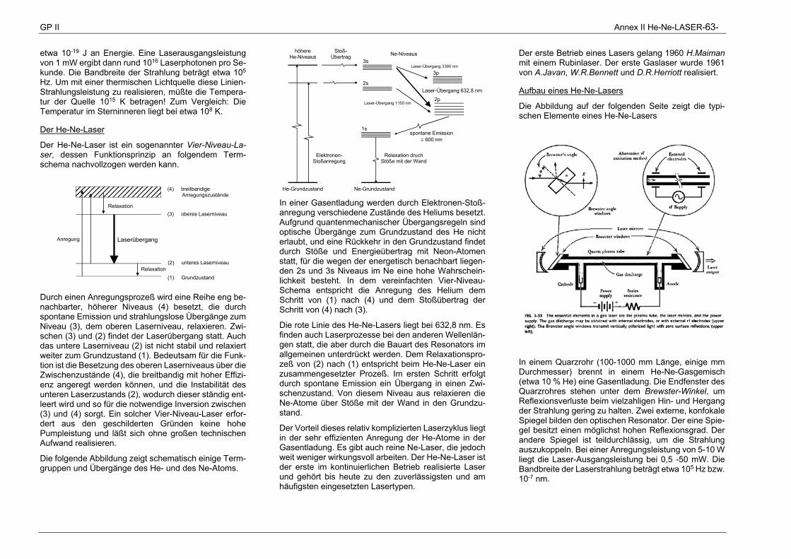
GP II Annex II He-Ne-LASER-63-

etwa 10-19 J an Energie. Eine Laserausgangsleistung von 1 mW ergibt dann rund 1016 Laserphotonen pro Se-kunde. Die Bandbreite der Strahlung beträgt etwa 105 Hz. Um mit einer thermischen Lichtquelle diese Linien-Strahlungsleistung zu realisieren, müßte die Tempera-tur der Quelle 1015 K betragen! Zum Vergleich: Die Temperatur im Sterninneren liegt bei etwa 108 K.

Der He-Ne-Laser

Der He-Ne-Laser ist ein sogenannter Vier-Niveau-La-ser, dessen Funktionsprinzip an folgendem Term-schema nachvollzogen werden kann.

Anregung

(4) breitbandige Anregungszustände

Relaxation

Relaxation

Laserübergang

(3) oberes Laserniveau

(2) unteres Laserniveau

(1) Grundzustand

Durch einen Anregungsprozeß wird eine Reihe eng be-nachbarter, höherer Niveaus (4) besetzt, die durch spontane Emission und strahlungslose Übergänge zum Niveau (3), dem oberen Laserniveau, relaxieren. Zwi-schen (3) und (2) findet der Laserübergang statt. Auch das untere Laserniveau (2) ist nicht stabil und relaxiert weiter zum Grundzustand (1). Bedeutsam für die Funk-tion ist die Besetzung des oberen Laserniveaus über die Zwischenzustände (4), die breitbandig mit hoher Effizi-enz angeregt werden können, und die Instabilität des unteren Laserzustands (2), wodurch dieser ständig ent-leert wird und so für die notwendige Inversion zwischen (3) und (4) sorgt. Ein solcher Vier-Niveau-Laser erfor-dert aus den geschilderten Gründen keine hohe Pumpleistung und läßt sich ohne großen technischen Aufwand realisieren.

Die folgende Abbildung zeigt schematisch einige Term-gruppen und Übergänge des He- und des Ne-Atoms.

höhereHe-Niveaus

3s

2s

1s

3p

2p

Stoß-Übertrag Ne-Niveaus

Laser-Übergang 1150 nm

Laser-Übergang 632,8 nm

Laser-Übergang 3390 nm

spontane Emission 600 nm

Relaxation druchStöße mit der Wand

Elektronen-Stoßanregung

He-Grundzustand Ne-Grundzustand In einer Gasentladung werden durch Elektronen-Stoß-anregung verschiedene Zustände des Heliums besetzt. Aufgrund quantenmechanischer Übergangsregeln sind optische Übergänge zum Grundzustand des He nicht erlaubt, und eine Rückkehr in den Grundzustand findet durch Stöße und Energieübertrag mit Neon-Atomen statt, für die wegen der energetisch benachbart liegen-den 2s und 3s Niveaus im Ne eine hohe Wahrschein-lichkeit besteht. In dem vereinfachten Vier-Niveau-Schema entspricht die Anregung des Helium dem Schritt von (1) nach (4) und dem Stoßübertrag der Schritt von (4) nach (3).

Die rote Linie des He-Ne-Lasers liegt bei 632,8 nm. Es finden auch Laserprozesse bei den anderen Wellenlän-gen statt, die aber durch die Bauart des Resonators im allgemeinen unterdrückt werden. Dem Relaxationspro-zeß von (2) nach (1) entspricht beim He-Ne-Laser ein zusammengesetzter Prozeß. Im ersten Schritt erfolgt durch spontane Emission ein Übergang in einen Zwi-schenzustand. Von diesem Niveau aus relaxieren die Ne-Atome über Stöße mit der Wand in den Grundzu-stand.

Der Vorteil dieses relativ komplizierten Laserzyklus liegt in der sehr effizienten Anregung der He-Atome in der Gasentladung. Es gibt auch reine Ne-Laser, die jedoch weit weniger wirkungsvoll arbeiten. Der He-Ne-Laser ist der erste im kontinuierlichen Betrieb realisierte Laser und gehört bis heute zu den zuverlässigsten und am häufigsten eingesetzten Lasertypen.

Der erste Betrieb eines Lasers gelang 1960 H.Maiman mit einem Rubinlaser. Der erste Gaslaser wurde 1961 von A.Javan, W.R.Bennett und D.R.Herriott realisiert.

Aufbau eines He-Ne-Lasers

Die Abbildung auf der folgenden Seite zeigt die typi-schen Elemente eines He-Ne-Lasers

In einem Quarzrohr (100-1000 mm Länge, einige mm Durchmesser) brennt in einem He-Ne-Gasgemisch (etwa 10 % He) eine Gasentladung. Die Endfenster des Quarzrohres stehen unter dem Brewster-Winkel, um Reflexionsverluste beim vielzahligen Hin- und Hergang der Strahlung gering zu halten. Zwei externe, konfokale Spiegel bilden den optischen Resonator. Der eine Spie-gel besitzt einen möglichst hohen Reflexionsgrad. Der andere Spiegel ist teildurchlässig, um die Strahlung auszukoppeln. Bei einer Anregungsleistung von 5-10 W liegt die Laser-Ausgangsleistung bei 0,5 -50 mW. Die Bandbreite der Laserstrahlung beträgt etwa 105 Hz bzw. 10-7 nm.

GP Annex III CURRENT CONDITION -64

64

Anlage III STROMLEITUNG GP II

Die Beschreibung der Stromleitung in Festkörpern er-folgt im Rahmen der Festkörperphysik durch quanten-mechanische Vorstellungen. Einige wesentliche As-pekte sollen hier phänomenologisch und qualitativ aus-führlicher dargestellt werden, da das Thema einen Vor-griff auf den Stoff späterer Vorlesungen darstellt.

Atom

Bei freien Atomen bewirkt der positiv geladene Kern eine Potentialmulde, in der im neutralen Fall sämtliche Elektronen des Atoms fest gebunden sind. Analog zu den diskreten Schwingungsfrequenzen einer beidseitig eingespannten Saite führt die räumliche Begrenzung der Elektronen auf das Atomvolumen dazu, daß nur ganz bestimmte Zustände mit diskreten Energien und Drehimpulsen eingenommen werden können (Bohr'sches Atommodell). Zustände mit unterschiedli-chem Drehimpuls, aber eng benachbarten Energien, werden zu Schalen zusammengefaßt (Hauptquanten-zahlen). Nach dem Pauli-Prinzip darf jeder Zustand nur mit (höchstens) einem Elektron besetzt werden, so daß mit steigender Kernladungszahl Z immer höhere Scha-len aufgefüllt werden. Die am schwächsten gebunde-nen Elektronen in der äußersten Schale (d.h. die mit der höchsten Energie) bestimmen den chemischen Charak-ter des Elements (Leuchtelektron). Das Periodensys-tem der Elemente in der Anordnung mit steigendem Z spiegelt diese Schalenstruktur wieder.

Elektronen in Festkörpern

Bei der Kondensation von Atomen zu einem Festkörper (z.B. Kupfer mit Z=29 zu Cu-Metall) können sich die Po-tentiale benachbarter Atome deformieren und soweit überlappen, daß der höchste besetzte Zustand ober-halb der einzelnen Potentialmulden liegt. Damit sind die Elektronen in diesem Zustand nicht mehr an das Atom gebunden, und zurück bleiben Cu+-Ionen und die unge-bundene Elektronen als sogenanntes Elektronengas. Die Bildung eines derartigen Elektronengases hoher Dichte (etwa ein Elektron pro Atom, d.h. etwa 1029 m-3 für Kupfer) ist das Kennzeichen eines Metalls. Typische metallische Eigenschaften, wie z.B. die hohe elektri-

sche und thermische Leitfähigkeit und das große Ab-sorptions- und Reflexionsvermögen für Licht, sind Ei-genschaften dieses Elektronengases. Allerdings sind die Elektronen nicht uneingeschränkt frei, sondern ihre Beweglichkeit unterliegt weiter dem Pauli-Prinzip, so daß Ortsveränderungen nur durch Platzwechsel auf freie Zustände erfolgen können.

Bandstruktur

Durch den Überlapp der Potentiale benachbarter Atome werden die Elektronen auf den äußeren Bahnen gekop-pelt, und es entsteht eine Aufspaltung (Vermehrung) der möglichen Zustände analog der Aufspaltung der Ei-genfrequenzen gekoppelter Pendel. Für einen Festkör-per mit einer sehr großen Zahl von N gekoppelten Ato-men liegen die Zustände so dicht beieinander, daß man sie für viele Betrachtungen als quasi kontinuierlich ver-teilt ansehen kann und von einem (Energie-) Band spricht. Atomare Zustände, die sich nur durch die Ori-entierung des Drehimpulses unterscheiden, bilden ge-meinsame Bänder. Grundsätzlich sind jedoch auch die Zustände in den Bändern diskret und können, entspre-chend dem Pauli-Prinzip, nur mit je einem Elektron be-setzt sein, wobei die Anzahl der Zustände in einem Band gleich der Zahl der beteiligten Zustände pro Atom mal der Anzahl der Atome N ist. Zwischen den Bändern können Bandlücken (verbotene Zonen) liegen.

Leiter

Die äußeren Elektronen von Kupfer sind s-Elektronen mit zwei Drehimpulsorientierungen, so daß es 2N Lei-tungsband-Zustände gibt, die von den N Leitungselekt-ronen (eins je Atom) also gerade zur Hälfte aufgefüllt werden. Derartige nicht vollständig besetzte Bänder werden als Leitfähigkeits- oder kurz Leitungsbänder be-zeichnet, weil in diesen freie Plätze (Zustände) vorhan-den sind, über die eine einseitige Elektronenbewegung, und damit ein Ladungstransport stattfinden kann.

Die Elektronen in den höchsten besetzten Bandzustän-den an der Fermigrenze besitzen relativ hohe kineti-sche Energien mit Geschwindigkeiten von etwa 106 m/s (bei rein klassischer Betrachtungsweise eines Elektro-nengases würde dies einer Temperatur von 105 K ent-sprechen). Daran gemessen ist die zusätzliche Be-schleunigungsenergie durch ein äußeres elektrisches Feld vergleichsweise klein, so daß nur die "obersten" Elektronen in freie Zustände angehoben werden und

zum Ladungstransport beitragen können. Alle anderen dagegen (99% bei Zimmertemperatur) verbleiben in ih-ren Zuständen und tragen nicht zum Ladungsstrom (und auch nicht zum Wärmetransport und zur Wärme-kapazität) bei.

Nichtleiter

Werden pro Atom genau so viele Elektronen freigesetzt (delokalisiert), wie Zustände in einem Band enthalten sind, so wird das Band vollständig gefüllt. Es gibt keine freien Zustände, und damit ist eine Aufnahme elektri-scher Feldenergie und eine elektrische Leitung nicht möglich; der Festkörper ist ein Isolator. Derartige voll-ständig besetzten Bänder heißen Valenzbänder.

Halbleiter

Liegt das nächsthöhere, leere Band nur in geringem Energieabstand über dem gefüllten Valenzband, so können durch thermische Anregung Elektronen aus dem Valenzband über die Bandlücke E gehoben wer-den, und das leere Band wird zum Leitungsband. Zu-sätzlich hinterlassen die angehobenen Elektronen Lü-cken (Löcher) im Valenzband, also freie Zustände, so daß auch darin ein Ladungstransport möglich wird. Die Substanz wird zum Halbleiter (genauer Eigenhalbleiter oder intrinsischer Halbleiter). Nach allgemeinen Geset-zen der Thermodynamik wird der Bruchteil der angeho-benen Elektronen durch den Boltzmannfaktor kTEG /e (k = Boltzmannkonstante) bestimmt. (Wie groß ist die-ser Faktor für Germanium mit EG = 0,6 eV bei Zimmer-temperatur?).

Störstellenhalbleiter (Dotierung)

Die spezifische Leitfähigkeit ist proportional zur La-dungsträgerdichte, bei einem intrinsischen Halbleiter also exponentiell mit der Temperatur wachsend. Hö-here und bei Raumtemperatur praktisch konstante La-dungsträgerdichten erhält man durch Dotierung mit Ato-men anderer Wertigkeit. Durch die Fremdatome entste-hen besetzte Zustände in der Bandlücke des Halbleiters dicht unterhalb des Leitungsbandes bzw. freie Zu-stände dicht oberhalb des Valenzbandes, die ein zu-sätzliches Elektron abgeben (Donatoren) oder aufneh-men (Akzeptoren) können, und die wegen ihrer gerin-gen Anregungsenergie bereits bei Zimmertemperatur vollständig angeregt bzw. besetzt sind.

GP II Annex III CURRENT CONDITION-65-

Elektrischer Widerstand

Die Stromleitung in einem Metall und dessen elektri-scher Widerstand lassen sich in einfacher Näherung klassisch verständlich machen. Wird an dem Metall durch Verbinden mit einer Spannungsquelle ein elektri-sches Feld erzeugt, so versetzt dies die freien Elektro-nen in beschleunigte Bewegungen, die durch Stöße mit den Ion-Rümpfen immer wieder unterbrochen werden. Es stellt sich eine im statistischen Mittel gleichförmige Bewegung mit einer mittleren Driftgeschwindigkeit ein, die proportional zur Spannung ist, und die sich aus der Teilchenzahldichte, der Ladung und der Stromdichte berechnen läßt. Aus diesem Bild folgt das Ohmsche Gesetz mit R = const.

Dies klassische Bild besitzt aber Grenzen, und erst die Quantenmechanik erklärt, wie sich Elektronen in einem räumlich periodischen Potential ohne Streuung bewe-gen können, d.h. ohne (wie klassisch zu erwarten) mit den Atomrümpfen zusammenzustoßen. Ein ideal auf-gebautes Metallgitter ohne Störungen der Periodizität durch Fremdatome oder durch thermischen Schwin-gungen der Ionen (am Temperatur-Nullpunkt) hat da-nach keinen elektrischen Widerstand (dies ist nicht die Supraleitung).

Bei Zimmertemperatur ist die mit der Temperatur zu-nehmende thermische Bewegung als Ursache für den Widerstand dominierend, der beim Abkühlen auf sehr tiefe Temperaturen für reine Metalle typisch um einen Faktor 100 sinkt. Der schließlich temperaturunabhän-gige Restwiderstand ist ein Maß für die Reinheit des Materials. Bei Legierungen dagegen kann der Fehlstel-lenbeitrag so groß werden, daß er schon bei Raumtem-peratur überwiegt. Dies Verhalten erklärt den hohen spezifischen Widerstand von z.B. Manganin und Kon-stantan und dessen geringe Temperaturabhängigkeit.

Supraleitung

Grund der Supraleitung ist nicht die Verringerung der thermischen Schwingungen bei tiefen Temperaturen als eine der Ursachen des Widerstands, sondern eine Zustandsänderung des Elektronengases durch Bildung sogenannter Cooper-Paare durch eine sehr schwache Phononen-Austauschwechselwirkung zwischen Elekt-ronen entgegengerichteten Spins, wobei sich die elekt-ronischen Eigenschaften grundlegend ändern und die

Gitterstörungen als Ursachen des Widerstands von den Elektronen nicht mehr wahrgenommen werden.

Im Normalzustand unterliegen Elektronen als Spin-1/2-Teilchen der Fermi-Statistik und sind als kleine Teilchen zu verstehen, die im Wellenbild eine kurze (de-Broglie-) Wellenlänge besitzen. Durch die Kopplung werden die Cooper-Paare spinlos. Sie folgen dann der Bose-Ein-stein-Statistik und nicht mehr dem Pauli-Prinzip, und können einen einheitlichen, kohärenten Zustand bilden, der sich durch eine große de-Broglie-Wellenlänge aus-zeichnet. In diesem Zustand nehmen die Elektronen die thermischen Gitterschwingungen der Atomrümpfe und auch Gitter-Fehlstellen als räumlich kleine Störungen nicht mehr wahr, und es kommt zu dem Effekt des ver-schwindenden Widerstands.

Die Kopplung zu Cooper-Paaren ist in einem Elektro-nengas innerhalb eines Gitters möglich, da dort die Coulomb-Wechselwirkung durch die allseitige Umge-bung mit gleich geladenen Teilchen nahezu völlig aus-geschaltet ist, und unterhalb einer bestimmten Tempe-ratur (der Sprungtemperatur), wenn auch die thermi-schen Phononen ausreichend abgeschwächt sind. Die innere Energie des Metalls ist dann umso kleiner, je mehr Cooper-Paare gebildet werden, so daß sie den energetisch günstigstens Zustand des Systems darstel-len. Es handelt sich dabei um eine Phasenänderung des Systems, die nicht in Abhängigkeit der Temperatur verläuft, sondern sprungartig, und bei der sich die Ent-ropie des Systems unstetig ändert.

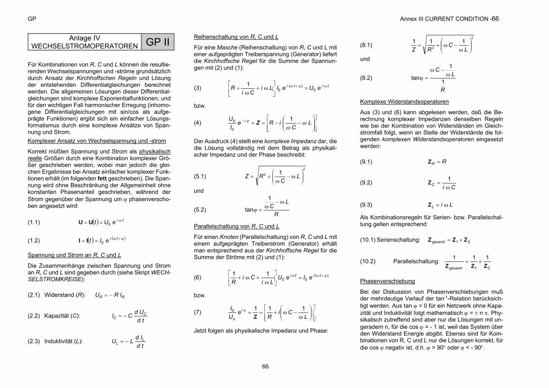
GP Annex III CURRENT CONDITION -66

66

Anlage IV WECHSELSTROMOPERATOREN GP II

Für Kombinationen von R, C und L können die resultie-renden Wechselspannungen und -ströme grundsätzlich durch Ansatz der Kirchhoffschen Regeln und Lösung der entstehenden Differentialgleichungen berechnet werden. Die allgemeinen Lösungen dieser Differential-gleichungen sind komplexe Exponentialfunktionen, und für den wichtigen Fall harmonischer Erregung (inhomo-gene Differentialgleichungen mit sin/cos als aufge-prägte Funktionen) ergibt sich ein einfacher Lösungs-formalismus durch eine komplexe Ansätze von Span-nung und Strom. Komplexer Ansatz von Wechselspannung und -strom

Korrekt müßten Spannung und Strom als physikalisch reelle Größen durch eine Kombination komplexer Grö-ßer geschrieben werden, wobei man jedoch die glei-chen Ergebnisse bei Ansatz einfacher komplexer Funk-tionen erhält (im folgenden fett geschrieben). Die Span-nung wird ohne Beschränkung der Allgemeinheit ohne konstanten Phasenanteil geschrieben, während der Strom gegenüber der Spannung um phasenverscho-ben angesetzt wird:

(1.1) tieUt 0UU

(1.2) tieIt 0II

Spannung und Strom an R, C und L

Die Zusammenhänge zwischen Spannung und Strom an R, C und L sind gegeben durch (siehe Skript WECH-SELSTROMKREISE):

(2.1) Widerstand (R): RR IRU

(2.2) Kapazität (C): td

UdCI CC

(2.3) Induktivität (L): tdIdLU L

L

Reihenschaltung von R, C und L

Für eine Masche (Reihenschaltung) von R, C und L mit einer aufgeprägten Treiberspannung (Generator) liefert die Kirchhoffsche Regel für die Summe der Spannun-gen mit (2) und (1):

(3) titi eUeILiCi

R

0

)(0

1

bzw.

(4)

L

CiRe

IU i

1

0

0 Z

Der Ausdruck (4) stellt eine komplexe Impedanz dar, die die Lösung vollständig mit dem Betrag als physikali-scher Impedanz und der Phase beschreibt:

(5.1) 2

2 1

L

CRZ

und

(5.2) R

LC

1

tan

Parallelschaltung von R, C und L

Für einen Knoten (Parallelschaltung) von R, C und L mit einem aufgeprägten Treiberstrom (Generator) erhält man entsprechend aus der Kirchhoffsche Regel für die Summe der Ströme mit (2) und (1):

(6) )(00

11

titi eIeULi

CiR

bzw.

(7)

LCi

Re

UI i

o

1110

Z

Jetzt folgen als physikalische Impedanz und Phase:

(8.1) 2

2

111

L

CRZ

und

(8.2)

R

LC

1

1

tan

Komplexe Widerstandsoperatoren

Aus (3) und (6) kann abgelesen werden, daß die Be-rechnung komplexer Impedanzen denselben Regeln wie bei der Kombination von Widerständen im Gleich-stromfall folgt, wenn an Stelle der Widerstände die fol-genden komplexen Widerstandsoperatoren eingesetzt werden:

(9.1) RR Z

(9.2) CiC

1Z

(9.3) LiL Z

Als Kombinationsregeln für Serien- bzw. Parallelschal-tung gelten entsprechend:

(10.1) Serienschaltung: 21 ZZZ gesamt

(10.2) Parallelschaltung: 21

111ZZZ

gesamt

Phasenverschiebung

Bei der Diskussion von Phasenverschiebungen muß der mehrdeutige Verlauf der tan-1-Relation berücksich-tigt werden. Aus tan = 0 für ein Netzwerk ohne Kapa-zität und Induktivität folgt mathematisch = n . Phy-sikalisch zutreffend sind aber nur die Lösungen mit un-geradem n, für die cos = - 1 ist, weil das System über den Widerstand Energie abgibt. Ebenso sind für Kom-binationen von R, C und L nur die Lösungen korrekt, für die cos negativ ist, d.h. > 90 oder < - 90.

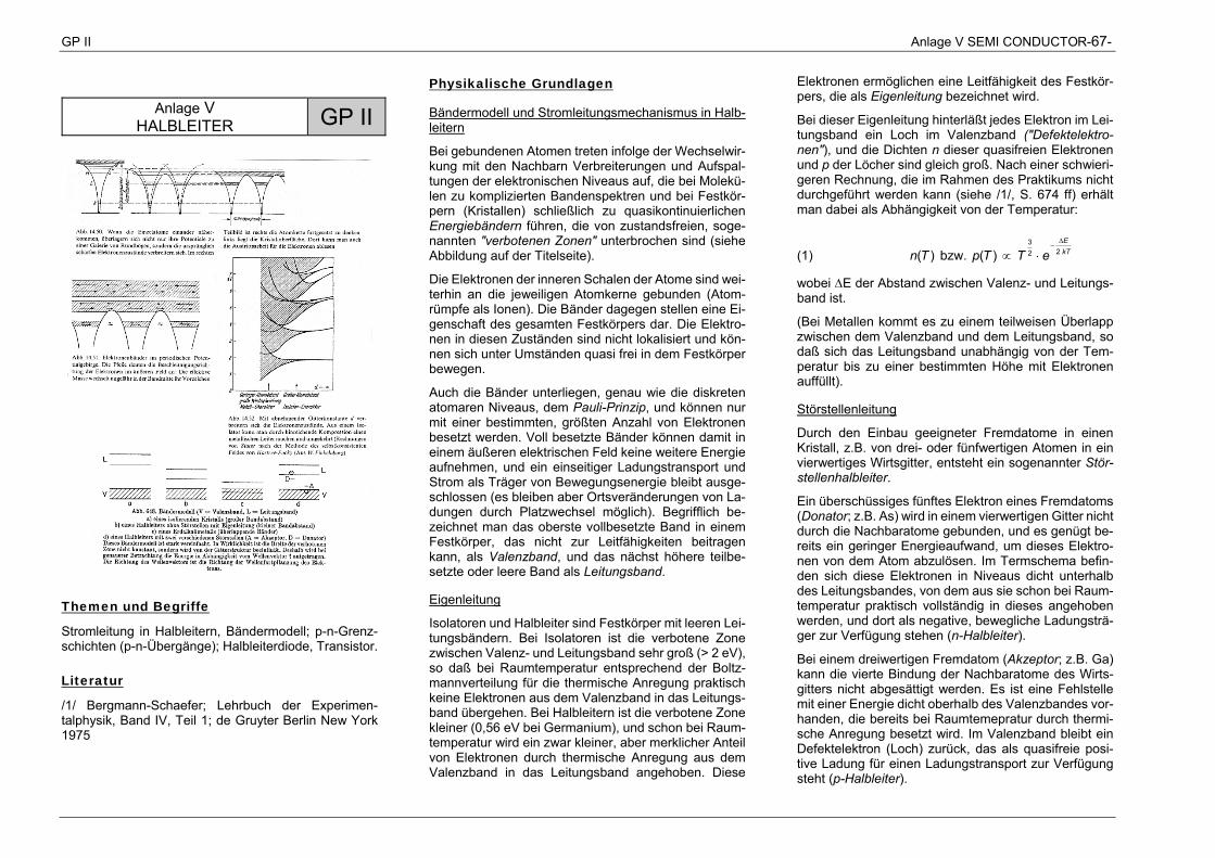
GP II Anlage V SEMI CONDUCTOR-67-

Anlage V HALBLEITER GP II

Themen und Begriffe

Stromleitung in Halbleitern, Bändermodell; p-n-Grenz-schichten (p-n-Übergänge); Halbleiterdiode, Transistor.

Literatur

/1/ Bergmann-Schaefer; Lehrbuch der Experimen-talphysik, Band IV, Teil 1; de Gruyter Berlin New York 1975

Physikalische Grundlagen

Bändermodell und Stromleitungsmechanismus in Halb-leitern

Bei gebundenen Atomen treten infolge der Wechselwir-kung mit den Nachbarn Verbreiterungen und Aufspal-tungen der elektronischen Niveaus auf, die bei Molekü-len zu komplizierten Bandenspektren und bei Festkör-pern (Kristallen) schließlich zu quasikontinuierlichen Energiebändern führen, die von zustandsfreien, soge-nannten "verbotenen Zonen" unterbrochen sind (siehe Abbildung auf der Titelseite).

Die Elektronen der inneren Schalen der Atome sind wei-terhin an die jeweiligen Atomkerne gebunden (Atom-rümpfe als Ionen). Die Bänder dagegen stellen eine Ei-genschaft des gesamten Festkörpers dar. Die Elektro-nen in diesen Zuständen sind nicht lokalisiert und kön-nen sich unter Umständen quasi frei in dem Festkörper bewegen.

Auch die Bänder unterliegen, genau wie die diskreten atomaren Niveaus, dem Pauli-Prinzip, und können nur mit einer bestimmten, größten Anzahl von Elektronen besetzt werden. Voll besetzte Bänder können damit in einem äußeren elektrischen Feld keine weitere Energie aufnehmen, und ein einseitiger Ladungstransport und Strom als Träger von Bewegungsenergie bleibt ausge-schlossen (es bleiben aber Ortsveränderungen von La-dungen durch Platzwechsel möglich). Begrifflich be-zeichnet man das oberste vollbesetzte Band in einem Festkörper, das nicht zur Leitfähigkeiten beitragen kann, als Valenzband, und das nächst höhere teilbe-setzte oder leere Band als Leitungsband.

Eigenleitung

Isolatoren und Halbleiter sind Festkörper mit leeren Lei-tungsbändern. Bei Isolatoren ist die verbotene Zone zwischen Valenz- und Leitungsband sehr groß (> 2 eV), so daß bei Raumtemperatur entsprechend der Boltz-mannverteilung für die thermische Anregung praktisch keine Elektronen aus dem Valenzband in das Leitungs-band übergehen. Bei Halbleitern ist die verbotene Zone kleiner (0,56 eV bei Germanium), und schon bei Raum-temperatur wird ein zwar kleiner, aber merklicher Anteil von Elektronen durch thermische Anregung aus dem Valenzband in das Leitungsband angehoben. Diese

Elektronen ermöglichen eine Leitfähigkeit des Festkör-pers, die als Eigenleitung bezeichnet wird.

Bei dieser Eigenleitung hinterläßt jedes Elektron im Lei-tungsband ein Loch im Valenzband ("Defektelektro-nen"), und die Dichten n dieser quasifreien Elektronen und p der Löcher sind gleich groß. Nach einer schwieri-geren Rechnung, die im Rahmen des Praktikums nicht durchgeführt werden kann (siehe /1/, S. 674 ff) erhält man dabei als Abhängigkeit von der Temperatur:

(1) kTE

eTTpTn 223

)( bzw. )(

wobei E der Abstand zwischen Valenz- und Leitungs-band ist.

(Bei Metallen kommt es zu einem teilweisen Überlapp zwischen dem Valenzband und dem Leitungsband, so daß sich das Leitungsband unabhängig von der Tem-peratur bis zu einer bestimmten Höhe mit Elektronen auffüllt).

Störstellenleitung

Durch den Einbau geeigneter Fremdatome in einen Kristall, z.B. von drei- oder fünfwertigen Atomen in ein vierwertiges Wirtsgitter, entsteht ein sogenannter Stör-stellenhalbleiter.

Ein überschüssiges fünftes Elektron eines Fremdatoms (Donator; z.B. As) wird in einem vierwertigen Gitter nicht durch die Nachbaratome gebunden, und es genügt be-reits ein geringer Energieaufwand, um dieses Elektro-nen von dem Atom abzulösen. Im Termschema befin-den sich diese Elektronen in Niveaus dicht unterhalb des Leitungsbandes, von dem aus sie schon bei Raum-temperatur praktisch vollständig in dieses angehoben werden, und dort als negative, bewegliche Ladungsträ-ger zur Verfügung stehen (n-Halbleiter).

Bei einem dreiwertigen Fremdatom (Akzeptor; z.B. Ga) kann die vierte Bindung der Nachbaratome des Wirts-gitters nicht abgesättigt werden. Es ist eine Fehlstelle mit einer Energie dicht oberhalb des Valenzbandes vor-handen, die bereits bei Raumtemepratur durch thermi-sche Anregung besetzt wird. Im Valenzband bleibt ein Defektelektron (Loch) zurück, das als quasifreie posi-tive Ladung für einen Ladungstransport zur Verfügung steht (p-Halbleiter).

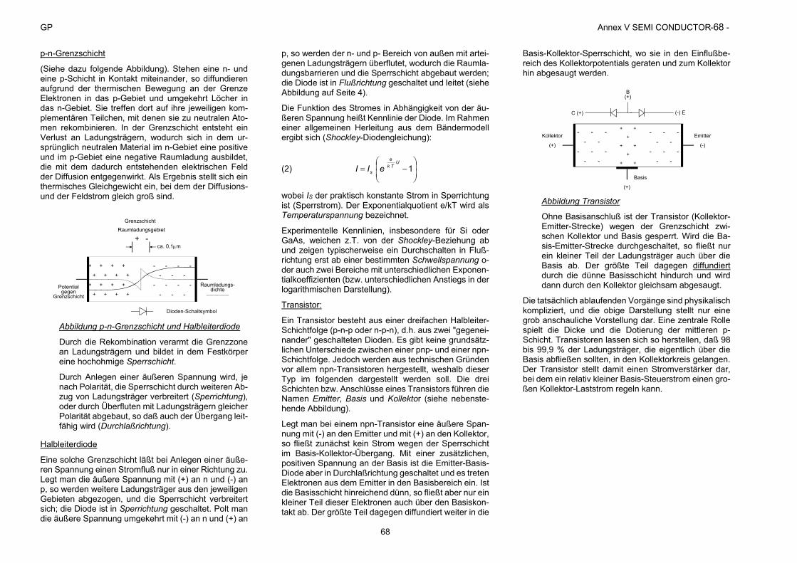
GP Annex V SEMI CONDUCTOR-68 -

68

p-n-Grenzschicht

(Siehe dazu folgende Abbildung). Stehen eine n- und eine p-Schicht in Kontakt miteinander, so diffundieren aufgrund der thermischen Bewegung an der Grenze Elektronen in das p-Gebiet und umgekehrt Löcher in das n-Gebiet. Sie treffen dort auf ihre jeweiligen kom-plementären Teilchen, mit denen sie zu neutralen Ato-men rekombinieren. In der Grenzschicht entsteht ein Verlust an Ladungsträgern, wodurch sich in dem ur-sprünglich neutralen Material im n-Gebiet eine positive und im p-Gebiet eine negative Raumladung ausbildet, die mit dem dadurch entstehenden elektrischen Feld der Diffusion entgegenwirkt. Als Ergebnis stellt sich ein thermisches Gleichgewicht ein, bei dem der Diffusions- und der Feldstrom gleich groß sind.

+ + + +

+ + + +

+ + + +

+ + + +

- - - -- - -

- - - -- - -

Grenzschicht

ca. 0,1m

Raumladungsgebiet

+ -

Dioden-Schaltsymbol

Potentialgegen

Grenzschicht

Raumladungs-dichte

Abbildung p-n-Grenzschicht und Halbleiterdiode

Durch die Rekombination verarmt die Grenzzone an Ladungsträgern und bildet in dem Festkörper eine hochohmige Sperrschicht.

Durch Anlegen einer äußeren Spannung wird, je nach Polarität, die Sperrschicht durch weiteren Ab-zug von Ladungsträger verbreitert (Sperrichtung), oder durch Überfluten mit Ladungsträgern gleicher Polarität abgebaut, so daß auch der Übergang leit-fähig wird (Durchlaßrichtung).

Halbleiterdiode

Eine solche Grenzschicht läßt bei Anlegen einer äuße-ren Spannung einen Stromfluß nur in einer Richtung zu. Legt man die äußere Spannung mit (+) an n und (-) an p, so werden weitere Ladungsträger aus den jeweiligen Gebieten abgezogen, und die Sperrschicht verbreitert sich; die Diode ist in Sperrichtung geschaltet. Polt man die äußere Spannung umgekehrt mit (-) an n und (+) an

p, so werden der n- und p- Bereich von außen mit artei-genen Ladungsträgern überflutet, wodurch die Raumla-dungsbarrieren und die Sperrschicht abgebaut werden; die Diode ist in Flußrichtung geschaltet und leitet (siehe Abbildung auf Seite 4).

Die Funktion des Stromes in Abhängigkeit von der äu-ßeren Spannung heißt Kennlinie der Diode. Im Rahmen einer allgemeinen Herleitung aus dem Bändermodell ergibt sich (Shockley-Diodengleichung):

(2)

1

UTk

e

s eII

wobei IS der praktisch konstante Strom in Sperrichtung ist (Sperrstrom). Der Exponentialquotient e/kT wird als Temperaturspannung bezeichnet.

Experimentelle Kennlinien, insbesondere für Si oder GaAs, weichen z.T. von der Shockley-Beziehung ab und zeigen typischerweise ein Durchschalten in Fluß-richtung erst ab einer bestimmten Schwellspannung o-der auch zwei Bereiche mit unterschiedlichen Exponen-tialkoeffizienten (bzw. unterschiedlichen Anstiegs in der logarithmischen Darstellung).

Transistor:

Ein Transistor besteht aus einer dreifachen Halbleiter-Schichtfolge (p-n-p oder n-p-n), d.h. aus zwei "gegenei-nander" geschalteten Dioden. Es gibt keine grundsätz-lichen Unterschiede zwischen einer pnp- und einer npn-Schichtfolge. Jedoch werden aus technischen Gründen vor allem npn-Transistoren hergestellt, weshalb dieser Typ im folgenden dargestellt werden soll. Die drei Schichten bzw. Anschlüsse eines Transistors führen die Namen Emitter, Basis und Kollektor (siehe nebenste-hende Abbildung).

Legt man bei einem npn-Transistor eine äußere Span-nung mit (-) an den Emitter und mit (+) an den Kollektor, so fließt zunächst kein Strom wegen der Sperrschicht im Basis-Kollektor-Übergang. Mit einer zusätzlichen, positiven Spannung an der Basis ist die Emitter-Basis-Diode aber in Durchlaßrichtung geschaltet und es treten Elektronen aus dem Emitter in den Basisbereich ein. Ist die Basisschicht hinreichend dünn, so fließt aber nur ein kleiner Teil dieser Elektronen auch über den Basiskon-takt ab. Der größte Teil dagegen diffundiert weiter in die

Basis-Kollektor-Sperrschicht, wo sie in den Einflußbe-reich des Kollektorpotentials geraten und zum Kollektor hin abgesaugt werden.

- - - - -

- - - - -

- - - - -

- - - - -

+ +

+

+ +

+

+ +

B(+)

C (+) (-) E

Kollektor

(+)

Emitter

(-)

Basis

(+) Abbildung Transistor

Ohne Basisanschluß ist der Transistor (Kollektor-Emitter-Strecke) wegen der Grenzschicht zwi-schen Kollektor und Basis gesperrt. Wird die Ba-sis-Emitter-Strecke durchgeschaltet, so fließt nur ein kleiner Teil der Ladungsträger auch über die Basis ab. Der größte Teil dagegen diffundiert durch die dünne Basisschicht hindurch und wird dann durch den Kollektor gleichsam abgesaugt.

Die tatsächlich ablaufenden Vorgänge sind physikalisch kompliziert, und die obige Darstellung stellt nur eine grob anschauliche Vorstellung dar. Eine zentrale Rolle spielt die Dicke und die Dotierung der mittleren p-Schicht. Transistoren lassen sich so herstellen, daß 98 bis 99,9 % der Ladungsträger, die eigentlich über die Basis abfließen sollten, in den Kollektorkreis gelangen. Der Transistor stellt damit einen Stromverstärker dar, bei dem ein relativ kleiner Basis-Steuerstrom einen gro-ßen Kollektor-Laststrom regeln kann.

Documents

Freie Universität Berlin Department of Physics GPII Basic ... · Freie Universität Berlin Department of Physics Basic Laboratory Course in Physics ... and conducting an experiment