Embed Size (px)
Citation preview
J. Non-Newtonian Fluid Mech. 108 (2002) 363–409
Free surface flows of polymer solutions with modelsbased on the conformation tensor
Matteo Pasquali∗, L.E. ScrivenCoating Process Fundamentals Program, Department of Chemical Engineering and Materials Science, Center for Interfacial
Engineering, University of Minnesota Supercomputing Institute, University of Minnesota, Minneapolis, MN 55455, USA
Abstract
A computational method is presented for analyzing free surface flows of polymer solutions with the confor-mation tensor. It combines methods of computing Newtonian free surface flows [J. Comp. Phys. 99 (1992) 39;V.F. deAlmeida, Gas–Liquid Counterflow Through Constricted Passages, Ph.D. thesis, University of Minnesota,Minneapolis, MN, 1995 (Available from UMI, Ann Arbor, MI, order number 9615160); J. Comp. Phys. 125 (1996)83] and viscoelastic flows [J. Non-Newtonian Fluid Mech. 60 (1995) 27; J. Non-Newtonian Fluid Mech. 59 (1995)215]. Modifications are introduced to compute a traceless velocity gradient, to impose inflow boundary conditionson the conformation tensor that are independent of the specific model adopted, and to include traction boundaryconditions at free surfaces and open boundaries.
A new method is presented for deriving and coding the entries of the analytical Jacobian for Newton’s methodby keeping the derivatives of the finite element weighted residual equations with respect to the finite element basisfunctions in their natural vector and tensor forms, and then by mapping such vectors and tensors into the elementalJacobian matrix. A new definition of extensional and shear flow is presented that is based on projecting the rate ofstrain tensor onto the principal basis defined by the conformation tensor.
The method is validated with two benchmark problems: flow around a cylinder in a channel, and flow underthe downstream section of a slot or knife coater. Regions of molecular stretch—determined by monitoring theeigenvalues of the conformation tensor—and molecular extension and shear rate—determined by projecting therate of strain dyadic onto the eigenvectors of the conformation tensor—are shown in the flow around a cylinder ofan Oldroyd-B liquid.
The free surface coating flow between a moving rigid boundary and a parallel static solid boundary from whicha free surface detaches is analyzed with several models of dilute and semidilute solutions of polymer of varyingdegree of stiffness based on the conformation tensor approach [J. Non-Newtonian Fluid Mech. 23 (1987) 271; A.N.Beris, B.J. Edwards, Thermodynamics of Flowing Systems with Internal Microstructure, 1st ed., Oxford UniversityPress, Oxford, 1994; J. Rheol. 38 (1994) 769; M. Pasquali, Polymer Molecules in Free Surface Coating Flows,Ph.D. thesis, University of Minnesota, Minneapolis, MN, 2000 (Available from UMI, Ann Arbor, MI, order number9963019)].
∗ Corresponding author. Present address: Chemical Engineering Department, Rice University, MS 362, P.O. Box 1892, Houston,TX 77251-1892, USA.E-mail addresses:[email protected] (M. Pasquali), [email protected] (L.E. Scriven).
0377-0257/02/$ – see front matter © 2002 Elsevier Science B.V. All rights reserved.PII: S0377-0257(02)00138-6
364 M. Pasquali, L.E. Scriven / J. Non-Newtonian Fluid Mech. 108 (2002) 363–409
Although the boundary conditions at the static contact line introduce a singularity, that singularity does not affectthe computation of flows at high Weissenberg number when a recirculation is present under the static boundary. Inthis case, a steep layer of molecular stretch develops under the free surface downstream of the stagnation point. Herethe polymer aligns with its principal stretching axis parallel to the free surface. When the recirculation is absent, thesingularity at the contact line strongly affects the computed velocity gradient, and the computations fail at moderateWeissenberg number irrespective of the polymer model and of whether the polymer is affecting the flow or not.© 2002 Elsevier Science B.V. All rights reserved.
Keywords:Free surface flows; Polymer solutions; Conformation tensor; Viscoelastic flows; Flow type classification; Finiteelements
1. Introduction
Free surface flows and free boundary problems arise when one or more layers of liquids flow together,possibly meeting a gas at one or more interfaces, and possibly interacting with a deformable elastic solidat other interfaces. Such problems abound in coating (e.g. slot coating, deformable roll coating), polymerprocessing (e.g. extrusion, calendering), cell engineering (e.g. deformation of blood cells), hemodynamics(blood flow in arteries), and biomechanics and tissue engineering (lubrication flow in articular joints,carthilage deformation).
The mathematical modeling of free surface flows requires solving free boundary problems, i.e. prob-lems where the domain of definition of the differential equations describing the flow is unknown and itslocation must be part of the solution of the problem. Open flow boundaries are often present where theliquid enters or exits the flow domain; approximate boundary conditions are imposed there that are notdictated by the physics of the problem, but by the need of truncating the computational domain, and thesensitivity of the flow computations to the location of the open boundaries must be assessed and reducedto an acceptable level.
The methods used to compute Newtonian free surface flows are also applicable to viscoelastic freesurface flows. Different ways of handling free surface flows are discussed in detail by Kistler and Scriven[10,11], Christodoulou and Scriven[1], Christodoulou[12], deAlmeida[2,13] and Sackinger et al.[3].Such methods have been extended successfully to elastohydrodynamics problems, where a flowing New-tonian liquid interacts with a deformable elastic solid at common boundaries[14–16].
Computational methods to solve viscoelastic flows are still an active area of research, and severalmethods of solving the partial differential equations of such flows have been proposed in recent years(see[17] for a recent review). The method used here is a slight modification of the discrete elastico-viscoussplit stress, independent velocity gradient interpolation, streamline upwind Petrov–Galerkin (DEVSS-G/SUPG)[5], one of the youngest members of the family of methods of weighted residuals with finite elementbasis functions that originated in the elastico-viscous split stress (EVSS)[18]. The DEVSS-G/SUPGmethod and its variants are convergent and accurate at low and moderate values of the Weissenbergnumber[4,5,19–21].
The set of non-linear algebraic equations for the finite element basis functions that arises from applyingthe method of weighted residuals to the conservation equations of mass, momentum, and polymer confor-mation, together with the elliptic mesh generation equations and the appropriate boundary conditions, issolved by Newton’s method with analytical Jacobian and first-order arclength continuation in parameterspace[22].
M. Pasquali, L.E. Scriven / J. Non-Newtonian Fluid Mech. 108 (2002) 363–409 365
Because the number of scalar differential equations to solve is high (12 or 13 for two-dimensionalflows, 22 for three-dimensional flows), a large number of analytical derivatives must be calculated tocompute the analytical Jacobian. To reduce the number of analytical derivatives, the coefficients of thefinite element basis functions and the residual equations residuals of the elliptic mesh generation arekept in their natural vector or tensor form. The number of equations and unknowns is thereby reducedto 5 and the number of analytical derivatives needed drops accordingly, although these derivatives aretensor-valued.
The residual equations and Jacobian entries depend on the particular constitutive form of the free energyand the generation terms in the transport equation of conformation. A general method is developed ofwriting computer code that reflects the tensorial nature of the equations and unknown basis functioncoefficients, and that is independent of the particular constitutive choices, provided that the constitutiveequation belongs to the conformation tensor family[6–9], so that only few short user-specified routinesmust be changed to solve free surface flows of polymer solutions with different constitutive equations. Tomake the method fully general, a new way of imposing inflow boundary conditions on the conformationtensor (or elastic stress) is introduced that is independent of the choice of constitutive model.
The theory and computational method are applied to analyze coating flows of polymer solutions, forwhich there are very few results based on simplified one-dimensional analysis[23], asymptotic expansions[24], or early attempts at solving the two-dimensional free surface flow problem with the EVSS method[25]. In coating operations, the degree of stiffness of the polymer molecules dissolved in the coatingliquid ranges from low, as in aqueous solutions of polyethylene oxide, to high, as in solutions of xanthan[26], and may depend on the type of solvent surrounding the molecules, and on the concentration ofpolymer. Polymer concentrations range from few parts per million, as in some specialized precisioncoating operations, to almost pure polymer, as in hot-melt coating of low-molecular weight adhesives.Studying how different types of polymer molecules behave in coating flows in different concentrationregimes is therefore important.
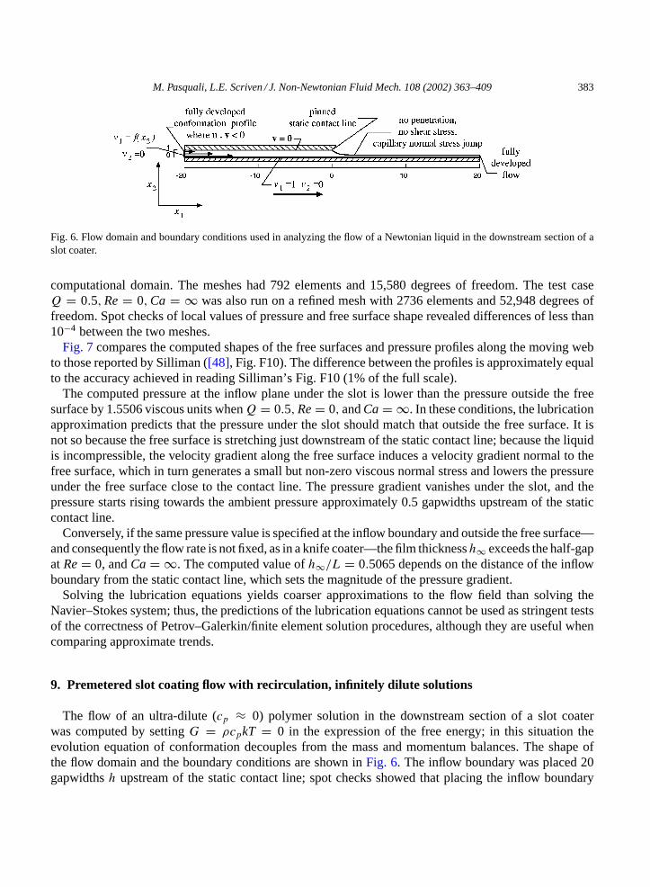
The interaction of flow and polymer microstructure is analyzed in the free surface flow between amoving rigid boundary and a parallel static solid boundary from which a free surface detaches (Fig. 6).This free surface flow is a prototype coating flow; it is the downstream section, or tail-end, of a slot coater,if the flow rate through the inflow boundary is fixed, i.e. the flow is premetered; and it is the downstreamsection of a knife coater, if the pressure difference between the inflow section and the gas outside the freesurface is fixed and the flow rate is allowed to change, i.e. the flow is self-metering.
The solutions considered are infinitely dilute, dilute, and semidilute in polymer, none of them entangled,so that their salient microstructural features can be modeled with a single variable, the conformationdyadic, or second-order tensor[6–9]. The polymer molecules are extensible, semiextensible, and rigidlinear molecules. The simple models used to capture these molecular characteristics in the equation ofchange of the conformation dyadic are described inSection 3below.
2. Elliptic mesh generation/domain deformation
To compute a free surface flow, the unknown flow domain (physical domain) is mapped into a fixedreference domain (computational domain). Common ways of constructing the mapping are the methodof spines[10,27]; the elliptic mesh generation method[1,12], where the mapping is the solution ofan elliptic differential equation; and the domain deformation method[2,3,13], where the mapping is
366 M. Pasquali, L.E. Scriven / J. Non-Newtonian Fluid Mech. 108 (2002) 363–409
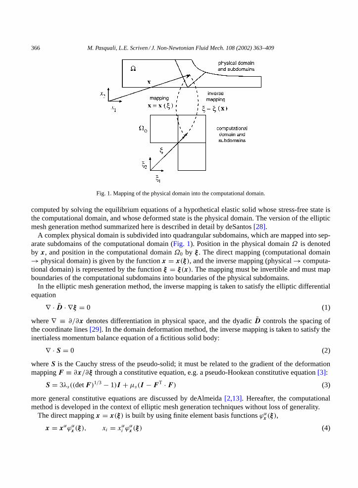
Fig. 1. Mapping of the physical domain into the computational domain.
computed by solving the equilibrium equations of a hypothetical elastic solid whose stress-free state isthe computational domain, and whose deformed state is the physical domain. The version of the ellipticmesh generation method summarized here is described in detail by deSantos[28].
A complex physical domain is subdivided into quadrangular subdomains, which are mapped into sep-arate subdomains of the computational domain (Fig. 1). Position in the physical domainΩ is denotedby x, and position in the computational domainΩ0 by ξ . The direct mapping (computational domain→ physical domain) is given by the functionx = x(ξ), and the inverse mapping (physical→ computa-tional domain) is represented by the functionξ = ξ(x). The mapping must be invertible and must mapboundaries of the computational subdomains into boundaries of the physical subdomains.
In the elliptic mesh generation method, the inverse mapping is taken to satisfy the elliptic differentialequation
∇ · D · ∇ξ = 0 (1)
where∇ ≡ ∂/∂x denotes differentiation in physical space, and the dyadicD controls the spacing ofthe coordinate lines[29]. In the domain deformation method, the inverse mapping is taken to satisfy theinertialess momentum balance equation of a fictitious solid body:
∇ · S = 0 (2)
whereS is the Cauchy stress of the pseudo-solid; it must be related to the gradient of the deformationmappingF ≡ ∂x/∂ξ through a constitutive equation, e.g. a pseudo-Hookean constitutive equation[3]:
S = 3λs((detF )1/3 − 1)I + µs(I − F T · F ) (3)
more general constitutive equations are discussed by deAlmeida[2,13]. Hereafter, the computationalmethod is developed in the context of elliptic mesh generation techniques without loss of generality.
The direct mappingx = x(ξ) is built by using finite element basis functionsϕαx (ξ),
x = xαϕαx (ξ), xi = xαi ϕαx (ξ) (4)
M. Pasquali, L.E. Scriven / J. Non-Newtonian Fluid Mech. 108 (2002) 363–409 367
wherexα is the set of unknown coefficients, and the indexi denotes direction in physical space. Einstein’ssummation convention over repeated Greek or italic indices is used hereafter. The subscript on the basisfunction denotes the variable that is approximated with that basis function; the Greek index identifieseach basis function in the basis set. The same basis functions are used for the components of the samevariable. The italic subscript or subscripts on the basis function coefficients represent vector or tensorcomponents in space, and the Greek superscripts identify each coefficient. The physical components ofthe approximated value of a variable are identified with italic subscripts and no superscript.
Boundary conditions used to solveEq. (1)are: (1)prescribed angle: the angleθ between the coordinateline ξi and the boundary is assigned,n · ∇ξi = |∇ξi | cosθ , i = 1 or 2; (2)slide over boundary: thenodes are free to slide on a line whose equation isf (x) = 0; (3) fixed nodes: the location of the nodeson the boundary is fixed,xα = xα, wherexα is the pre-assigned position of nodeα; (4) prescribed nodaldistribution: the nodes are distributed on the boundary of the physical domain according to a functiong
that controls their spacing,ξi = g(s), i = 1 or 2; (5)no-penetration(kinematic): the liquid cannot crossa free surface,n · v = 0.
3. Transport equations
The transport equations of mass, momentum, and conformation in a steady, isothermal, incompressible,non-diffusing flow of a non-entangled polymer solution are[9]:
0 = ∇ · v (5)
0 = ρv · ∇v − ∇ · T − ∇Θ (6)
0= v · ∇M − 2ξ
(D : M
I : MM
)
− ζ(
M · D + D · M − 2D : M
I : MM
)− M · W − WT · M + 1
λ(g0I + g1M + g2M
2) (7)
wherev is the liquid’s velocity,ρ the liquid’s density,T the stress tensor (Cauchy),Θ the potential ofthe body forces per unit volume,M the dimensionless conformation dyadic,D the rate of strain,W thevorticity dyadic, andλ is the characteristic relaxation time of the polymer. The constitutive functionξ(M)
represents the resistance of the polymer segments to stretching along their backbone,ζ(M) represents theresistance of the segments to relative rotation with respect to neighbors, andg0(M), g1(M), g2(M) definethe rate of relaxation of the polymer segments. The dimensionless conformation dyadic is used becausethe number of polymer segments per unit volume is constant if the polymer solution is not entangled and ifchemical reactions and polymer degradation are absent. The dimensionless conformation dyadic is relatedto the dimensional conformation dyadicM ≡ cp〈rr〉 by the relationM ≡ 3/(cpNl2)M = 3/(Nl2)〈rr〉wherecp is the number of polymer molecules per unit mass,N is the number of Kuhn steps per polymersegment[30], l is the length of a Kuhn step,r is the end-to-end connector of a segment, and〈·〉 denotesaverage over the distribution of orientations of segments. At equilibriumM = I .
The stress dyadicT is split into isotropic, viscous, and elastic components,
T = −pI + τ + σ (8)
368 M. Pasquali, L.E. Scriven / J. Non-Newtonian Fluid Mech. 108 (2002) 363–409
where the pressurep is constitutively indeterminate because the liquid is incompressible, the viscousstressτ obeys Newton’s law of viscosity,
τ = 2µD (9)
and the elastic stressσ follows the constitutive relation[9]:
σ = 2(ξ − ζ ) M
I : MM :
∂a
∂M+ 2ζM · ∂a
∂M(10)
wherea(T ,M) is the Helmholtz free energy per unit volume.A particular form of the constitutive functionsξ(M), ζ(M), g0(M), g1(M), g2(M), anda(T ,M)must
be chosen to compute the flow of a particular polymeric liquid. However, the computational methodand computer programs needed to perform the calculations are independent of the specific choice ofconstitutive functions, and they are developed in the general case. The different models of polymerbehavior used to analyze the free surface flow under a static edge are outlined here. These models may becrude approximations to how real polymer chains behave, but they do capture at least qualitatively someessential features and differences between polymers of different type.
3.1. Affinely deforming, infinitely extensible molecules (Gaussian)
Two hypotheses enter this model: (1) the molecules follow imposed larger-scale deformations affinely:ξ ≡ ζ ≡ 1; the rate of relaxation of the molecules is a linear function of the distance of the dimensionlessconformation tensorM from its equilibrium valueI : g0 ≡ −1, g1 ≡ 1, g2 ≡ 0. With these hypotheses,the evolution equation of the dimensionless conformation dyadic is
M ≡ ∂M
∂t+ v · ∇M = ∇vT · M + M · ∇v − 1
λ(M − I ) (11)
Eq. (11)yields the Upper Convected Maxwell model if the Helmholtz free energy per unit volume of theliquid depends linearly on the trace of the conformation dyadic,a ≡ (G/2)Tr M, and there is no viscousstress; it yields the Oldroyd-B model, if the stress has both an elastic and a viscous components.
The ratio of the volume pervaded by the molecules in the flow to the equilibrium value of their pervadedvolume is represented by the square root of the determinant of the conformation dyadic. In this model, itcan change by action of the velocity gradient.
3.2. Affinely deforming, finitely extensible molecules (FENE-P)
The hypothesis of the finitely extensible, non-linearly elastic (FENE) equations are: the moleculesfollow imposed deformations affinely:ξ ≡ ζ ≡ 1; the maximum extension of the molecules is finite, andtheir rate of relaxation grows infinitely fast as the average molecular extension approaches its maximumvalue:g0 ≡ −1,g1 ≡ (b−1)/(b−Tr M/3),g2 ≡ 0. The parameterb controls the molecular extensibility,and is defined as the ratio of the maximum length square of the polymer molecules to their average lengthsquare at equilibrium. The derivative ofg1 with respect to the conformation dyadic is needed to derivethe partial derivative entries in the Jacobian matrix needed for Newton’s method:
∂g1
∂Mij= 1
3
b − 1
(b − Tr (M/3))2δij (12)
M. Pasquali, L.E. Scriven / J. Non-Newtonian Fluid Mech. 108 (2002) 363–409 369
The evolution equation of the dimensionless conformation dyadic is
M ≡ ∂M
∂t+ v · ∇M = ∇vT · M + M · ∇v − 1
λ
(b − 1
b − Tr (M/3)M − I
)(13)
and the Helmholtz free energy is
a ≡ (3/2)G(b − 1)ln
[(b − 1)
(b − Tr (M/3)
]The non-linear relaxation term in the FENE-P equation puts a limit on the maximum extension achievableby the molecules, and is a significant improvement over its linear counterpart,Eq. (11). The FENE-Prelaxation function predicts that in a two-dimensional flow the polymer molecules contract in the neutraldirection of the flow[9]. Another variant of the FENE equations, the FENE-CR[31], does not have thisproperty because in the FENE-CR,g0 + g1 = 0.
3.3. Partially retracting semirigid molecules
The hypotheses of the model are: (1) the molecules follow imposed rotations affinely:ζ ≡ 1; (2) themolecules partially retract instantaneously if a sudden stretch is imposed along their axis, and the extentof the retraction is independent of the stretch of the molecules:ξ = constant< 1; (3) the rate of relaxationof the molecules is a linear function of the distance of the dimensionless conformation tensorM from itsequilibrium valueI : g0 ≡ −1, g1 ≡ 1, g2 ≡ 0. In this case, the evolution equation of the dimensionlessconformation dyadic is
M ≡ ∂M
∂t+ v · ∇M = 2ξ(M)
D : M
I : MM +
(M · D + D · M − 2
D : M
I : MM
)
+ M · W + WT · M − 1
λ(M − I ) (14)
and the Helmholtz free energy isa ≡ (G/2)(Tr M − ln detM).This model was introduced by Larson[32,33]and by Marrucci and Grizzuti[34] to describe the behavior
of entangled polymer segments that do not stretch along their backbone but orient collectively by followingthe imposed rotation[35]. Larson’s model captures some of the salient features of the reptation model,and like the reptation model describes reasonably well the near-linear behavior of entangled polymersolutions and melts in shear flow[36].
The partially retracting segment model describes well the behavior of rod-like polymer molecules thatare almost or completely rigid[35]; this is how the model is used here. If the stretching resistanceξ = 0,the retraction of the segments is complete and their length is constant; ifξ = 1, the molecules stretchwith the continuum deformation.
3.4. Boundary conditions on transport equations
Boundary conditions are needed on the momentum and conformation transport equations. The mo-mentum boundary conditions are:
(1) No-slip and no-penetration: At solid, impermeable boundaries, the velocity of the liquid equals thatof the solid,v = vw.
370 M. Pasquali, L.E. Scriven / J. Non-Newtonian Fluid Mech. 108 (2002) 363–409
(2) Force balance at free surfaces: The tangential traction vanishes at a free surface because the shearstress exerted by the gas on the liquid is negligible,tn : T = 0; the normal traction inside theliquid must balance the sum of the pressure in the gaspa and the capillary pressure induced by thecurvature of the surface,nn : T = −pa + ς∇II · n, whereς is the surface tension of the liquid, and∇II ≡ (I − nn) · ∇ is the surface gradient; in a two-dimensional flow, the normal stress balance canalso be written asnn : T = −pa + ςn · dt/ds, wheret is the tangent to the free surface, ands isarclength along the free surface—in vector form,n · T = −pan + ςdt/ds.
(3) Inflow and outflow conditions: A velocity profile is prescribed at the open boundary,v = v0(x),or a pressure datum is specified through the integral of the tractionn · t at the open boundary, orthe fully developed flow condition is imposed,n · ∇v = 0, also through the boundary integral ofthe traction. The former two boundary conditions are normally used at inflows, the latter at out-flows. Of course, the solution of the problem must prove insensitive to the location of the openboundaries.
(4) Symmetry: The liquid cannot cross a symmetry line or surface,n ·v = 0, and the shear stress vanishesthere,tn : T = 0.
The transport equation of conformationEq. (7)is hyperbolic and its characteristics in a steady flow arethe streamlines; therefore boundary conditions are needed only on inflow boundaries. BecauseEq. (7)is atensor equation, tensor boundary conditions must be imposed. The only exception is the flow of polymersolutions whose stress is purely elastic (τ = 0), where only the normal and tangential components of theconformation dyadic must be specified at the inflow boundaries[37,38].
The components of the conformation dyadic at an inflow boundary are not known in general. Com-monly, in viscoelastic flow computations the inflow boundaries are placed in regions of fully devel-oped, parallel, and rectilinear flow, where the profile of conformation is known analytically or itcan be computed in advance. Given a fixed inflow velocity profile, the inflow conformation profiledepends on the choice of constitutive functions in the transport equations; therefore the commonprocedure of imposing inflow boundary conditions on conformation is not amenable to genera-lization.
If the flow at the inflow boundary is fully developed, the conformation of the polymer there does notchange along the streamlines,v · ∇M = 0, and the algebraic equation
0= −2ξD : M
I : MM − ζ
(M · D + D · M − 2
D : M
I : MM
)
− M · W − WT · M + 1
λ(g0I + g1M + g2M
2) (15)
holds at the boundary.Eq. (15)is independent of constitutive assumptions and is enforced strongly astensor boundary condition at the inflow portions of open boundaries. Of course, an equivalent equationapplies if elastic stress rather than conformation is used as independent variable.
4. Modified transport equations
Three modifications to the transport equations are made before the equation set is cast in the weightedresidual form.
M. Pasquali, L.E. Scriven / J. Non-Newtonian Fluid Mech. 108 (2002) 363–409 371
4.1. Velocity gradient interpolation
As suggested by Szady et al.[5], an additional variableL is introduced to represent the velocity gradientwith a continuous interpolation:
0 = L − ∇v (16)
The variableL is calledinterpolated velocity gradientin the following to distinguish it from therawvelocity gradient∇v. The rate of strain dyadicD and the vorticity dyadicW in the transport equation ofconformation are computed using the interpolated velocity gradientL,
D ≡ 12(L + LT), W ≡ 1
2(L − LT) (17)
4.2. Traceless interpolated velocity gradient
In incompressible flows the trace of the velocity gradient vanishes,∇ ·v = Tr L = 0. The approximatevelocity field computed with the weighted residual/finite element method is not exactly divergence-free,and the approximate value of the interpolated velocity gradient is not exactly traceless. If the weightingfunctions used inEqs. (5) and (16)are different, the trace of the interpolated velocity gradient becomesdangerously large in flow regions where the velocity changes abruptly. TrL ≈ 0.1γmax is common oncoarse meshes, and TrL ≈ 0.01γmax is typical on more refined meshes (see[9] for details). Hereγmax
is the maximum of the positive eigenvalue of the rate of strain dyadic in the whole flow field.The rate of change along the streamlines of the determinant of the conformation dyadic is directly
related to TrL. The formula of the derivative of the determinant of a dyadic ([39], p. 26) andEq. (7)leadto the equation of change of the determinant of the conformation tensor,
D
Dtln detM = 6(ξ − ζ )D : M
I : M+ 2 TrD − 1
λ(g0 Tr M−1 + 3g1 + g2 Tr M) (18)
The determinant of the conformation dyadic must be positive becauseM is positive definite. If TrL iscomputed inaccurately, detM could change sign, leading to meaningless computational results. The traceof L can be computed accurately with the equation
0 = L − ∇v + 1
Tr I(∇ · v)I (19)
in place ofEq. (16). Eq. (19)guarantees that TrL = 0 regardless of the value of∇ · v.
4.3. Discrete adaptive viscous stress split
Guénette and Fortin[4] wrote the inertialess momentum equation as
∇ · (−pI + σ )+ ∇ · ηa(∇v + ∇vT − L − LT) = 0 (20)
whereηa is a numerical parameter, and showed that the last term inEq. (20)stabilized the computationalmethod. The assumption of Guénette and Fortin can also be explained by noting that either the raw, orthe interpolated velocity gradient, or a combination of both can be used to compute the viscous stress inEq. (9), and that the relation
τ = µ(L + LT)+ ηa(∇v + ∇vT − L − LT) (21)
together with the momentum transport equation leads toEq. (20).
372 M. Pasquali, L.E. Scriven / J. Non-Newtonian Fluid Mech. 108 (2002) 363–409
There is no difference between the interpretation ofEq. (20)given by Guénette and Fortin and thatoffered here withEq. (21)if velocity boundary conditions are imposed on the momentum equation onall boundaries, as is usually done in confined viscoelastic flows. However, the two interpretations lead todifferent ways of handling the traction boundary conditions used in free surface flows.
Interpreting the termηa(∇v + ∇vT − L − LT) as a stabilizing element in the momentum equationcompels that its boundary integral be accounted for at a free surface; conversely, defining the viscousstress withEq. (21)yields no contribution other than those of the ambient and capillary pressures to theboundary integral of the traction at a free surface. The latter approach is taken here. Computations weremade with a constant value ofηa. Changing the value ofηa had little or no effect on the solution of theflows, provided thatηa was comparable toµ.
5. Weighted residual equations
Multiplying Eqs. (1), (5)–(7), and(19), by weighting functionsψx, ψc, ψm, ψM , andψL, integratingover the (unknown) physical domainΩ (bounded byΓ ), applying the Gauss–Green–Ostrogradskii theo-rem to the mesh generation equation and to the momentum equation, and mapping the integrals onto the(known) computational domainΩ0 (bounded byΓ0) yields the weighted residual equations:
rx,α =∫Γ0
n · ψαx D · ∇ξ(dΓ0 −∫Ω0
∇ψαx · D · ∇ξf dΩ0 (22)
rc,α =∫Ω0
ψαc ∇ · vf dΩ0 (23)
rm,α =∫Ω0
ψαm (ρv · ∇v − ∇Θ)f dΩ0 +∫Ω0
∇ψαm · T f dΩ0 −∫Γ0
n · ψαmT (dΓ0 (24)
RL,α =∫Ω0
ψαL
(L − ∇v + 1
Tr I(∇ · v)I
)f dΩ0 (25)
RM,α =∫Ω0
ψαM
(v · ∇M − 2ξ
D : M
I : MM − ζ
(M · D + D · M − 2
D : M
I : MM
)
− M · W − WT · M + 1
λ(g0I + g1M + g2M
2)
)f dΩ0 (26)
n is the outward pointing normal to the boundaryΓ ;
( ≡ dΓ
dΓ0= detF
√n0 · KT · K · n0 (27)
is the ratio of the magnitudes of infinitesimal elements of boundary of the physical and computationaldomain ;n0 is the outward pointing unit normal to the computational domain,n = (f/()K · n0;
f ≡ dΩ
dΩ0= detF (28)
M. Pasquali, L.E. Scriven / J. Non-Newtonian Fluid Mech. 108 (2002) 363–409 373
is the Jacobian of the mapping, and represents the ratio of magnitudes of infinitesimal elements of thephysical and computational domains;
F ≡ x ≡ ∂x
∂ξ≡ ϕβx xβ, Fij ≡ ∂xj
∂ξi≡ i xj ≡ xβj
∂ϕβx
∂ξi(29)
is the mapping deformation gradient; denotes the gradient in the computational domain;1 and the indicesi, j denote direction in physical space.
The gradient in physical space∇ is related to the gradient in computational space by the relation
∇G = K · G, ∇iG ≡ ∂G
∂xi= Kij
∂G
∂ξj≡ Kij j G (30)
whereG can be any physical quantity—scalar, vector, dyadic, or tensor component—andK is the inversemapping deformation gradient,
K ≡ ∇ξ ≡ ∂ξ
∂x= F−1, Kij ≡ ∂ξj
∂xi(31)
Each independent variable is approximated with a linear combination of finite number of basis functionsx ≡ xβϕ
βx , p ≡ pβϕ
βp , v ≡ vβϕ
βv , L ≡ Lβϕ
β
L, andM ≡ Mβϕβ
M ; to lighten the notation, the samesymbolsx, p, v,L, andM are used to represent the approximate value of the independent variables, asin Eqs. (22)–(26), and their exact value, as inEqs. (1), (5)–(7), and(19). The context makes clear whetherthe exact or approximate value is referenced.
The basis functions used to represent the independent variables are: Lagrangian biquadratic for position(ϕx) and velocity (ϕv), linear discontinuous for pressure (ϕp), and Lagrangian bilinear for interpolatedvelocity gradient (ϕL) and conformation (ϕM ). Galerkin weighting functions are used in the residualequations of mesh generation (ψx ≡ ϕx), continuity (ψc ≡ ϕp), momentum (ψm ≡ ϕv), and velocitygradient interpolation (ψL ≡ ϕL), whereas streamline upwind Petrov–Galerkin weighting functionsare used in the conformation transport equation (ψM ≡ ϕM + huv · ∇ϕM ), wherehu is the upwindparameter—the characteristic size of the smallest element in the mesh.
6. Newton’s method with analytical Jacobian
The system of non-linear algebraic equationsEqs. (22)–(26) is solved with Newton’s method withanalytical Jacobian. The tolerance on the 2-norm of the residual and Newton update was set to 10−6. Thelinear system was solved with a frontal solver based on the algorithm of Duff et al.[9,43].
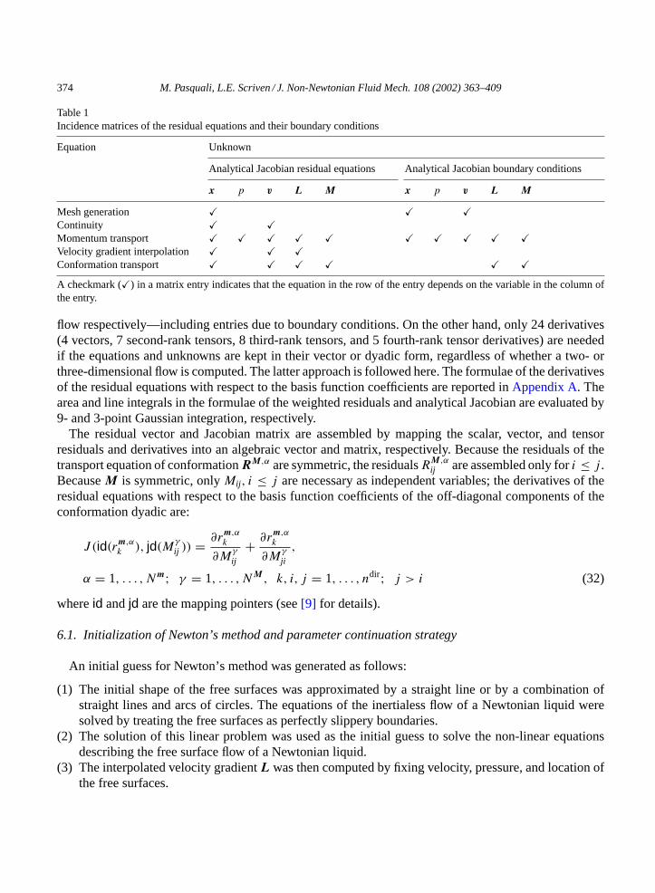
The formulae of the analytical derivatives ofEqs. (22)–(26)and their boundary conditions with respectto the basis function coefficientsxβ, pβ, vβ,Lβ , andMβ must be evaluated to compute the entriesof the Jacobian matrix.Table 1shows the incidence matrices ofEqs. (22)–(26) and their boundaryconditions. If each physical component of the residual equations and each component of the unknownvariables is considered a separate scalar, as is commonly done, the equation set has 13 equations in 13unknowns in a two-dimensional flow, and 22 equations in as many unknowns in a three-dimensionalflow, which leads to approximately 180 and 520 non-zero derivatives in a two- and three-dimensional
1 The symbol was originally used by Hamilton[40,41] to represent the gradient of a quaternion[42].
374 M. Pasquali, L.E. Scriven / J. Non-Newtonian Fluid Mech. 108 (2002) 363–409
Table 1Incidence matrices of the residual equations and their boundary conditions
Equation Unknown
Analytical Jacobian residual equations Analytical Jacobian boundary conditions
x p v L M x p v L M
Mesh generation Continuity Momentum transport Velocity gradient interpolation Conformation transport A checkmark () in a matrix entry indicates that the equation in the row of the entry depends on the variable in the column ofthe entry.
flow respectively—including entries due to boundary conditions. On the other hand, only 24 derivatives(4 vectors, 7 second-rank tensors, 8 third-rank tensors, and 5 fourth-rank tensor derivatives) are neededif the equations and unknowns are kept in their vector or dyadic form, regardless of whether a two- orthree-dimensional flow is computed. The latter approach is followed here. The formulae of the derivativesof the residual equations with respect to the basis function coefficients are reported inAppendix A. Thearea and line integrals in the formulae of the weighted residuals and analytical Jacobian are evaluated by9- and 3-point Gaussian integration, respectively.
The residual vector and Jacobian matrix are assembled by mapping the scalar, vector, and tensorresiduals and derivatives into an algebraic vector and matrix, respectively. Because the residuals of thetransport equation of conformationRM,α are symmetric, the residualsRM,α
ij are assembled only fori ≤ j .BecauseM is symmetric, onlyMij , i ≤ j are necessary as independent variables; the derivatives of theresidual equations with respect to the basis function coefficients of the off-diagonal components of theconformation dyadic are:
J (id(rm,αk ), jd(Mγ
ij )) = ∂rm,αk
∂Mγ
ij
+ ∂rm,αk
∂Mγ
ji
,
α = 1, . . . , Nm; γ = 1, . . . , NM , k, i, j = 1, . . . , ndir; j > i (32)
whereid andjd are the mapping pointers (see[9] for details).
6.1. Initialization of Newton’s method and parameter continuation strategy
An initial guess for Newton’s method was generated as follows:
(1) The initial shape of the free surfaces was approximated by a straight line or by a combination ofstraight lines and arcs of circles. The equations of the inertialess flow of a Newtonian liquid weresolved by treating the free surfaces as perfectly slippery boundaries.
(2) The solution of this linear problem was used as the initial guess to solve the non-linear equationsdescribing the free surface flow of a Newtonian liquid.
(3) The interpolated velocity gradientL was then computed by fixing velocity, pressure, and location ofthe free surfaces.
M. Pasquali, L.E. Scriven / J. Non-Newtonian Fluid Mech. 108 (2002) 363–409 375
(4) The polymer conformation dyadicM was then computed by fixing velocity, pressure, location of thefree surfaces, and interpolated velocity gradient at a low value of the Weissenberg number, typicallyWs= 0.01, using the initial guessM = I for the polymer conformation dyadic (M = I + 2WsD isa more accurate initial guess; however the simpler initial guessM = I was always inside the radiusof convergence of Newton’s method in the cases examined).
The values of velocity, pressure, location of the free surfaces, interpolated velocity gradient, and polymerconformation so computed are those that occur in the flow of an infinitely dilute solution of polymer witha finite relaxation time and infinitely small elastic modulus, where there is no coupling between themomentum equation and the polymer conformation dyadic. The solution of this last problem provided arobust initial guess with which to compute the free surface flow of a polymer solution.
Solutions at different values of parameters were then generated with first-order arclength continuation[22]. The size of the continuation step was doubled automatically if Newton’s method converged in threeiterations or less, and was quartered if Newton’s method converged in more than six iterations, if it failedto converge, if the mesh folded, or if the conformation dyadic lost positive definiteness anywhere in theflow domain.
7. Indicators of local molecular and flow behavior
7.1. Molecular stretch and orientation
The solutions of equations of viscoelastic flow are often reported by showing the distributions ofCartesian components of the elastic stress dyadic. These distributions are difficult to interpret becausethe relationship between the Cartesian components of the stress dyadic and the microstructural state ofthe polymer is not immediately apparent.
The invariants of the conformation dyadic are immediately accessible measures of the microstructuralstate of the polymer in various regions of the flow. They are excellent means of displaying the results ofviscoelastic flow calculations.
The orthonormal eigenvectorsmi of the conformation dyadic represent the three mutually orthogonaldirections along which molecules are oriented and stretched, or contracted—the principal directions ofthe second moment of the distribution of stretch and orientation. The eigenvaluesmi represent the squareof the principal stretch ratios of flowing ensembles of polymer segments, i.e. the average length square ofpolymer segments along the principal directions of stretch divided by the length square of the segmentsat equilibrium. The square root of the determinant ofM is the ratio of the volume pervaded by theflowing molecules to the volume pervaded by the molecules at equilibrium. The eigenvalues ofM arealways real and positive becauseM is symmetric and positive definite. Hereafter, the convention is usedm1 ≤ m2 ≤ m3 to order the eigenvalues of conformation.
7.2. Molecular extension and shear rate
The classical definitions of shear and extension rates ([44], p.155, p. 162) are based on the Cartesiancomponents of the velocity gradient referred to conveniently chosen spatially uniform orthonormal basisvectors; they cannot be applied to flow where the velocity gradient is not homogeneous.
376 M. Pasquali, L.E. Scriven / J. Non-Newtonian Fluid Mech. 108 (2002) 363–409
The invariants of the rate of strain cannot serve as indicators of the type of flow because they do not carryany information on whether polymer molecules are being strained persistently along the same axes—theessence of extensional flow—or are rotating with respect to the principal axes of the rate of strain, so thateach molecule is alternatively elongated and contracted by the rate of strain—the essence of shear flow.The vorticity depends on the choice of frame of reference, and by itself cannot provide indications onthe local type of flow, although relative rotation rates defined as the difference between the vorticity andother rates of rotation have been used to index the flow type[45,46]. The invariants of the conformationdyadic (or elastic stress) cannot be used to index the local flow type because they contain information onthe whole upstream history of deformation and because they are affected by the intensity of the strainingas well as the type of deformation.
The chief difference between extensional and shear flows is that in extension polymer molecules arebeing stretched along the preferred direction(s) of stretch and orientation, and are being contracted alongthe direction(s) where they are already contracted and least likely to be oriented, whereas in a shear flowthe principal directions of stretching do not coincide with the principal directions of molecular stretch andorientation. This important physical difference suggests defining a mean ensemble molecular extensionrate as the rate of strain along the eigenvectorm3 associated with the largest eigenvalue ofM:
εM ≡ m3m3 : D (33)
The molecular extension rateεM is independent of choice of frame of reference. WhereεM > 0, polymersegments are being stretched along their direction of preferred stretch and orientation and the flow isworking against the molecular relaxation processes; whereεM < 0, the flow and the relaxation processeswork together towards restoring the equilibrium length of the polymer segments, i.e. the liquid is recoiling.
The molecular shear rate is defined as the rate of strain alongm1 of molecules aligned withm3:
γM ≡ |m1m3 : D| (34)
becauseD is symmetric,γM is also the rate of strain alongm3 of molecules aligned withm1. The absolutevalue appears inEq. (34)becausem1,−m1,m3, and−m3 are unit eigenvectors of the conformation dyadic,but the definition ofγM must be independent of the sign ofm1 andm3. A largeγM indicates that the rateof strain is deforming molecules aligned along one of the principal directions of the conformation tensorin a direction orthogonal to their orientation; it is stretching or contracting along their axes the moleculesthat are aligned at 45 with respect to the principal directions of the conformation tensor.
In two-dimensional, incompressible flows there is only one independent molecular extension rate andone independent molecular shear rate, whereas in three-dimensional flows there are two independentmolecular extension rates and three independent molecular shear rates; they coincide, respectively withthe diagonal and off-diagonal entries of the matrix of components ofD in a curvilinear orthogonalcoordinate system whose basis coincides locally with the eigenvectors ofM everywhere in the flow.
The molecular extension and shear rates can be used to define extensional and shear flow indices:
e ≡ ε21,M + ε2
2,M + ε23,M
−2IID
, s ≡ γ 212,M + γ 2
23,M + γ 231,M
−IID
, e + s = 1 (35)
In two-dimensional flows,Eq. (35)simplifies to
e ≡ ε2M
d2, s ≡ γ 2
M
d2(36)
whered is the positive eigenvalue ofD.
M. Pasquali, L.E. Scriven / J. Non-Newtonian Fluid Mech. 108 (2002) 363–409 377
The extension and shear flow indicators defined byEq. (35)are always well-defined because ifIID
vanishes, the whole rate of strain dyadic must vanish too.When applied to homogeneous extensional flow, the flow indicators signal that the flow is purely
extensional (e = 1, s = 0). However, in simple shear flow their values depend on both the choiceof model and the Weissenberg number because these determine the orientation of the eigenvectors ofthe conformation dyadic. At low Weissenberg number,e approaches unity whereass nearly vanishesbecauseM ≈ I + 2WsD and thus the eigenvectors ofM andD coincide. At high Weissenberg numberthe eigenvectors ofM tend to align with the velocity (m3) and the gradient (m1); thuse → 0 ands → 1.
Although the flow indicators,Eq. (35), do not classify shear flows according to the traditional definitions(i.e. independent of model and Weissenberg number), they give more faithful information on the couplingof flow and polymer behavior than the traditional definitions. The linearized version ofEq. (7)at lowWeissenberg number is
Ws(−v · ∇M + ∇vT · M + M · ∇v)− (M − I ) = 0
settingM ≡ I + εM, whereε is a small parameter, yields
2WsD − εM︸ ︷︷ ︸first order
+ εWs(−v · ∇M + D · M + M · D + WT · M + M · W )︸ ︷︷ ︸second order
= 0 (37)
i.e. the vorticity enters the equation of change ofM at second order. In physical terms, at lowWs thepolymer is nearly undistorted and thus it does not feel the vorticity and behaves as if it were in extensionalflow.
8. Comparison with published studies on confined viscoelastic flowsand Newtonian free surface flows
The equations of the theory were programmed in a Fortran 90 computational code (see[9] for de-tails). The correctness of the computer code was checked by comparing the analytical Jacobian to acentered-difference numerical Jacobian; by monitoring the quadratic convergence 2-norm of the residualvector in the terminal Newton iterations; by compiling the code on seven different computer systems andsolving the same problem; and by solving a number of problems whose solution could be checked againstindependently obtained solutions.
Some computations in the early stages of development of the code were made with the numericalJacobian in place of the analytical Jacobian. The time to compute the numerical Jacobian was large;moreover, loss of quadratic convergence at moderate values of the Weissenberg number was observedwhen a numerical Jacobian was used (see[9] for details).
8.1. Flow around a cylinder between parallel fixed planes
The flow of a Newtonian liquid and an Oldroyd-B liquid around a cylinder between parallel fixed planeswas analyzed, and the drag force on the cylinder was calculated and compared to the analytical solutionof Faxén[47], and to the finite element solution of Sun et al.[21].
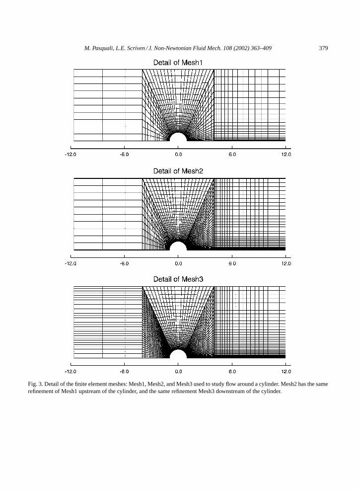
The flow domain, meshes, and boundary conditions are shown inFigs. 2 and 3. The ratio of cylinderdiameter to slit width was set to 1/8, as in[21]. The location of the inflow and outflow boundaries coincides
378 M. Pasquali, L.E. Scriven / J. Non-Newtonian Fluid Mech. 108 (2002) 363–409
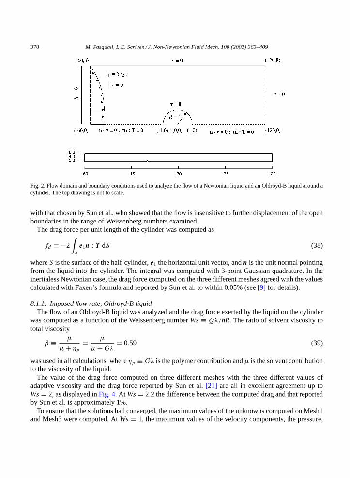
Fig. 2. Flow domain and boundary conditions used to analyze the flow of a Newtonian liquid and an Oldroyd-B liquid around acylinder. The top drawing is not to scale.
with that chosen by Sun et al., who showed that the flow is insensitive to further displacement of the openboundaries in the range of Weissenberg numbers examined.
The drag force per unit length of the cylinder was computed as
fd ≡ −2∫S
e1n : T dS (38)
whereS is the surface of the half-cylinder,e1 the horizontal unit vector, andn is the unit normal pointingfrom the liquid into the cylinder. The integral was computed with 3-point Gaussian quadrature. In theinertialess Newtonian case, the drag force computed on the three different meshes agreed with the valuescalculated with Faxen’s formula and reported by Sun et al. to within 0.05% (see[9] for details).
8.1.1. Imposed flow rate, Oldroyd-B liquidThe flow of an Oldroyd-B liquid was analyzed and the drag force exerted by the liquid on the cylinder
was computed as a function of the Weissenberg numberWs≡ Qλ/hR. The ratio of solvent viscosity tototal viscosity
β ≡ µ
µ+ ηp = µ
µ+Gλ = 0.59 (39)
was used in all calculations, whereηp ≡ Gλ is the polymer contribution andµ is the solvent contributionto the viscosity of the liquid.
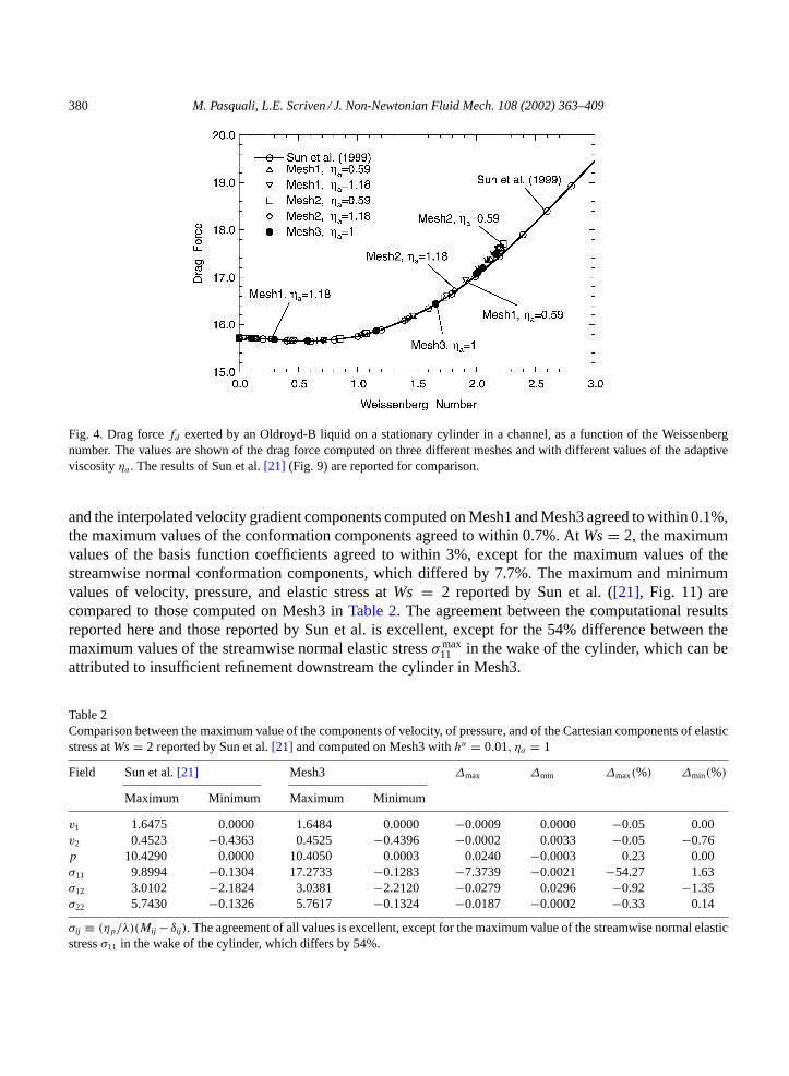
The value of the drag force computed on three different meshes with the three different values ofadaptive viscosity and the drag force reported by Sun et al.[21] are all in excellent agreement up toWs= 2, as displayed inFig. 4. At Ws= 2.2 the difference between the computed drag and that reportedby Sun et al. is approximately 1%.
To ensure that the solutions had converged, the maximum values of the unknowns computed on Mesh1and Mesh3 were computed. AtWs= 1, the maximum values of the velocity components, the pressure,
M. Pasquali, L.E. Scriven / J. Non-Newtonian Fluid Mech. 108 (2002) 363–409 379
Fig. 3. Detail of the finite element meshes: Mesh1, Mesh2, and Mesh3 used to study flow around a cylinder. Mesh2 has the samerefinement of Mesh1 upstream of the cylinder, and the same refinement Mesh3 downstream of the cylinder.
380 M. Pasquali, L.E. Scriven / J. Non-Newtonian Fluid Mech. 108 (2002) 363–409
Fig. 4. Drag forcefd exerted by an Oldroyd-B liquid on a stationary cylinder in a channel, as a function of the Weissenbergnumber. The values are shown of the drag force computed on three different meshes and with different values of the adaptiveviscosityηa . The results of Sun et al.[21] (Fig. 9) are reported for comparison.
and the interpolated velocity gradient components computed on Mesh1 and Mesh3 agreed to within 0.1%,the maximum values of the conformation components agreed to within 0.7%. AtWs= 2, the maximumvalues of the basis function coefficients agreed to within 3%, except for the maximum values of thestreamwise normal conformation components, which differed by 7.7%. The maximum and minimumvalues of velocity, pressure, and elastic stress atWs = 2 reported by Sun et al. ([21], Fig. 11) arecompared to those computed on Mesh3 inTable 2. The agreement between the computational resultsreported here and those reported by Sun et al. is excellent, except for the 54% difference between themaximum values of the streamwise normal elastic stressσmax
11 in the wake of the cylinder, which can beattributed to insufficient refinement downstream the cylinder in Mesh3.
Table 2Comparison between the maximum value of the components of velocity, of pressure, and of the Cartesian components of elasticstress atWs= 2 reported by Sun et al.[21] and computed on Mesh3 withhu = 0.01, ηa = 1
Field Sun et al.[21] Mesh3 ∆max ∆min ∆max(%) ∆min(%)
Maximum Minimum Maximum Minimum
v1 1.6475 0.0000 1.6484 0.0000 −0.0009 0.0000 −0.05 0.00v2 0.4523 −0.4363 0.4525 −0.4396 −0.0002 0.0033 −0.05 −0.76p 10.4290 0.0000 10.4050 0.0003 0.0240 −0.0003 0.23 0.00σ11 9.8994 −0.1304 17.2733 −0.1283 −7.3739 −0.0021 −54.27 1.63σ12 3.0102 −2.1824 3.0381 −2.2120 −0.0279 0.0296 −0.92 −1.35σ22 5.7430 −0.1326 5.7617 −0.1324 −0.0187 −0.0002 −0.33 0.14
σij ≡ (ηp/λ)(Mij − δij ). The agreement of all values is excellent, except for the maximum value of the streamwise normal elasticstressσ11 in the wake of the cylinder, which differs by 54%.
M. Pasquali, L.E. Scriven / J. Non-Newtonian Fluid Mech. 108 (2002) 363–409 381
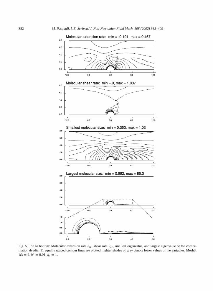
8.1.2. Portraits of flow characteristics and molecular properties at Ws= 2At Ws= 2 the streamlines differ only slightly from the Newtonian pattern. The highest rate of strain
is attained at the waist of the cylinder, where the distance between the cylinder and the channel wallis smallest.Fig. 5 (top) shows contours of molecular extension and shear rate, defined inSection 7.2.The molecular extension rate is the highest near the upstream stagnation point on the cylinder, wherethe molecules orient perpendicular to the stagnation streamline and stretch across and contract alongthe upstream stagnation streamline; and in the wake of the cylinder by the downstream stagnation point,where the molecules stretch and orient along and contract across the stagnation streamline. The molecularshear rate is the highest at the waist of the cylinder, where the rate of strain is the highest.
Fig. 5 (bottom) shows the eigenvalues of the conformation dyadic—the squared molecular stretches.On the upstream stagnation streamline, the molecules contract in the streamwise direction and stretchin the cross-stream direction. The molecules are most distorted in the wake downstream of the cylinder;the highest molecular distortion is 14.66 and occurs 0.912 cylinder radii downstream of the cylinder.The molecules shrink first in the cross-stream direction, then elongate in the streamwise direction as theydepart the downstream stagnation point and traverse the wake of the cylinder. The high values of moleculardistortion computed are partly due to the extreme molecular compliance built into the Oldroyd-B equation.The Oldroyd-B equation yields a degenerate behavior in uniaxial as well as planar steady extensionalflow, where it predicts infinite stresses at finite value of the Weissenberg number,Ws= 1/2 ([36], p. 26);in the computation atWs= 2 on the finest mesh, the flow at the midplane in the cylinder’s wake is planarextensional, and the local Weissenberg numberλL11 exceeds the critical value 1/2 in the third elementdownstream of the cylinder (x1 ≈ 1.033R), where the convective term is small (v1 ≈ 0.0049Q/h) andthus the behavior of the equation approaches that of steady flow.
The Oldroyd-B model is built by assuming that polymer molecules follow sudden imposed strainsand relax at a rate which is linearly proportional to their stretch: these hypotheses approximate poorlythe behavior of strongly stretched and oriented molecules, and the computed distributions of molecularstretch shown inFig. 5likely overpredict the distributions of stretch that a real solution of flexible polymercoils would attain.
8.2. Downstream section of a slot coater
The equation system describing the flow of a Newtonian liquid in the downstream section of a slotcoater was solved to test the correctness of the mesh generation equations and the free surface boundaryconditions. The Galerkin/finite element solution was computed as the flow of a polymer solution withno elasticity, i.e.Eqs. (22)–(24) were solved with the constitutiveEq. (8)of the total stress,(10) of theelastic stress, together witha = 0, and(21)of the viscous stress, withηa = µ = 1.Fig. 6shows the flowdomain and the boundary conditions used.
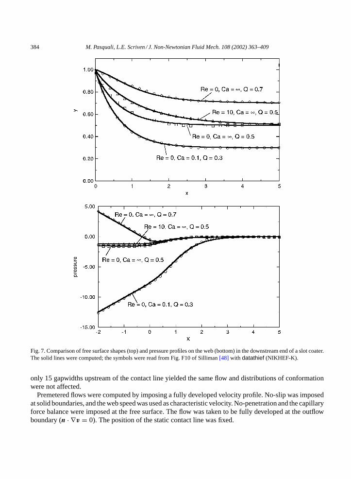
Four test cases were chosen to compare the results with those of Silliman[48]: (1) Q = 0.3,Re =0,Ca = 0.1; (2)Q = 0.5,Re = 0,Ca = ∞; (3) Q = 0.5,Re = 10,Ca = ∞; (4) Q = 0.7,Re =0,Ca = ∞; whereRe≡ ρvL/µ is the Reynolds number,Ca ≡ µv/ς is the capillary number, andQ isthe flow rate per unit width of the slot. The unit of velocityv is the web speed, and the unit of lengthLis the height of the gap between the slot die and the web.
The sensitivity of the flow to location of the open boundaries upstream and downstream was assessedby doubling the upstream and downstream length of the flow domain. The solutions computed on thetwo domains agreed to within 0.04%; therefore, all subsequent solutions were computed on the shorter
382 M. Pasquali, L.E. Scriven / J. Non-Newtonian Fluid Mech. 108 (2002) 363–409
Fig. 5. Top to bottom: Molecular extension rateεM , shear rateγM , smallest eigenvalue, and largest eigenvalue of the confor-mation dyadic. 11 equally spaced contour lines are plotted; lighter shades of gray denote lower values of the variables. Mesh3,Ws= 2, hu = 0.01, ηa = 1.
M. Pasquali, L.E. Scriven / J. Non-Newtonian Fluid Mech. 108 (2002) 363–409 383
Fig. 6. Flow domain and boundary conditions used in analyzing the flow of a Newtonian liquid in the downstream section of aslot coater.
computational domain. The meshes had 792 elements and 15,580 degrees of freedom. The test caseQ = 0.5,Re= 0,Ca = ∞ was also run on a refined mesh with 2736 elements and 52,948 degrees offreedom. Spot checks of local values of pressure and free surface shape revealed differences of less than10−4 between the two meshes.
Fig. 7compares the computed shapes of the free surfaces and pressure profiles along the moving webto those reported by Silliman ([48], Fig. F10). The difference between the profiles is approximately equalto the accuracy achieved in reading Silliman’s Fig. F10 (1% of the full scale).
The computed pressure at the inflow plane under the slot is lower than the pressure outside the freesurface by 1.5506 viscous units whenQ = 0.5,Re= 0,andCa = ∞. In these conditions, the lubricationapproximation predicts that the pressure under the slot should match that outside the free surface. It isnot so because the free surface is stretching just downstream of the static contact line; because the liquidis incompressible, the velocity gradient along the free surface induces a velocity gradient normal to thefree surface, which in turn generates a small but non-zero viscous normal stress and lowers the pressureunder the free surface close to the contact line. The pressure gradient vanishes under the slot, and thepressure starts rising towards the ambient pressure approximately 0.5 gapwidths upstream of the staticcontact line.
Conversely, if the same pressure value is specified at the inflow boundary and outside the free surface—and consequently the flow rate is not fixed, as in a knife coater—the film thicknessh∞ exceeds the half-gapat Re= 0, andCa = ∞. The computed value ofh∞/L = 0.5065 depends on the distance of the inflowboundary from the static contact line, which sets the magnitude of the pressure gradient.
Solving the lubrication equations yields coarser approximations to the flow field than solving theNavier–Stokes system; thus, the predictions of the lubrication equations cannot be used as stringent testsof the correctness of Petrov–Galerkin/finite element solution procedures, although they are useful whencomparing approximate trends.
9. Premetered slot coating flow with recirculation, infinitely dilute solutions
The flow of an ultra-dilute (cp ≈ 0) polymer solution in the downstream section of a slot coaterwas computed by settingG = ρcpkT = 0 in the expression of the free energy; in this situation theevolution equation of conformation decouples from the mass and momentum balances. The shape ofthe flow domain and the boundary conditions are shown inFig. 6. The inflow boundary was placed 20gapwidthsh upstream of the static contact line; spot checks showed that placing the inflow boundary
384 M. Pasquali, L.E. Scriven / J. Non-Newtonian Fluid Mech. 108 (2002) 363–409
Fig. 7. Comparison of free surface shapes (top) and pressure profiles on the web (bottom) in the downstream end of a slot coater.The solid lines were computed; the symbols were read from Fig. F10 of Silliman[48] with datathief (NIKHEF-K).
only 15 gapwidths upstream of the contact line yielded the same flow and distributions of conformationwere not affected.
Premetered flows were computed by imposing a fully developed velocity profile. No-slip was imposedat solid boundaries, and the web speed was used as characteristic velocity. No-penetration and the capillaryforce balance were imposed at the free surface. The flow was taken to be fully developed at the outflowboundary (n · ∇v = 0). The position of the static contact line was fixed.
M. Pasquali, L.E. Scriven / J. Non-Newtonian Fluid Mech. 108 (2002) 363–409 385
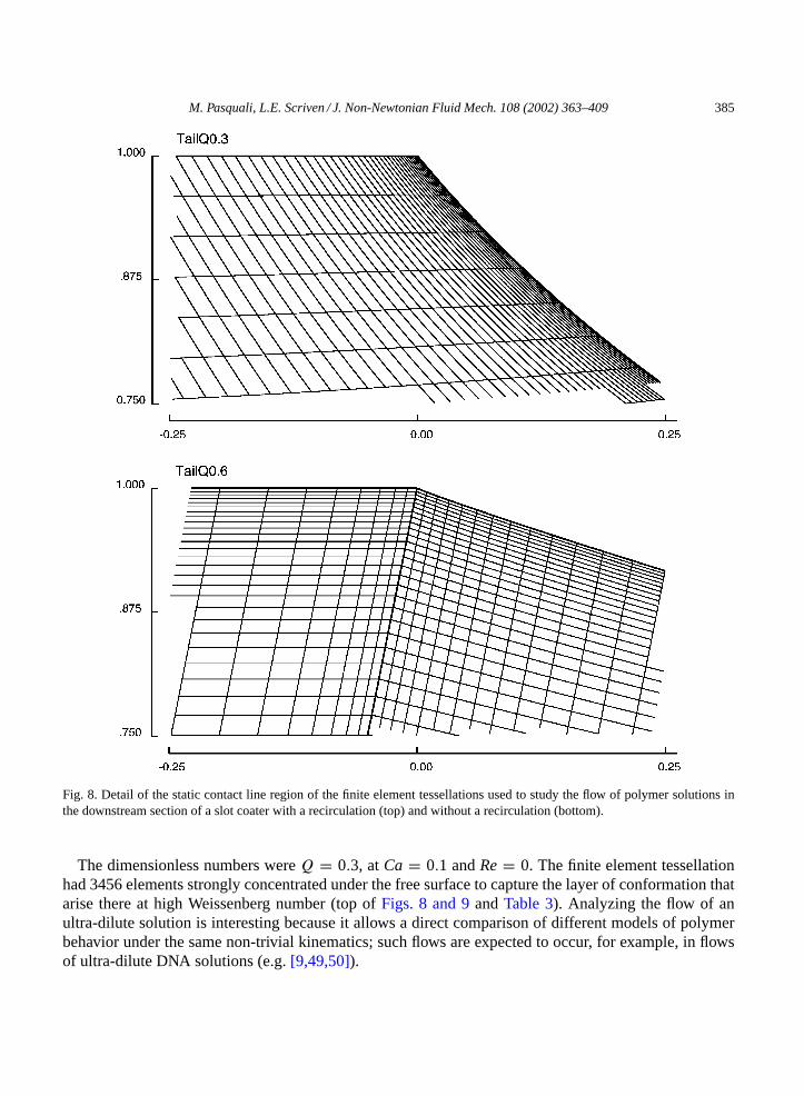
Fig. 8. Detail of the static contact line region of the finite element tessellations used to study the flow of polymer solutions inthe downstream section of a slot coater with a recirculation (top) and without a recirculation (bottom).
The dimensionless numbers wereQ = 0.3, atCa = 0.1 andRe= 0. The finite element tessellationhad 3456 elements strongly concentrated under the free surface to capture the layer of conformation thatarise there at high Weissenberg number (top ofFigs. 8 and 9andTable 3). Analyzing the flow of anultra-dilute solution is interesting because it allows a direct comparison of different models of polymerbehavior under the same non-trivial kinematics; such flows are expected to occur, for example, in flowsof ultra-dilute DNA solutions (e.g.[9,49,50]).
386 M. Pasquali, L.E. Scriven / J. Non-Newtonian Fluid Mech. 108 (2002) 363–409
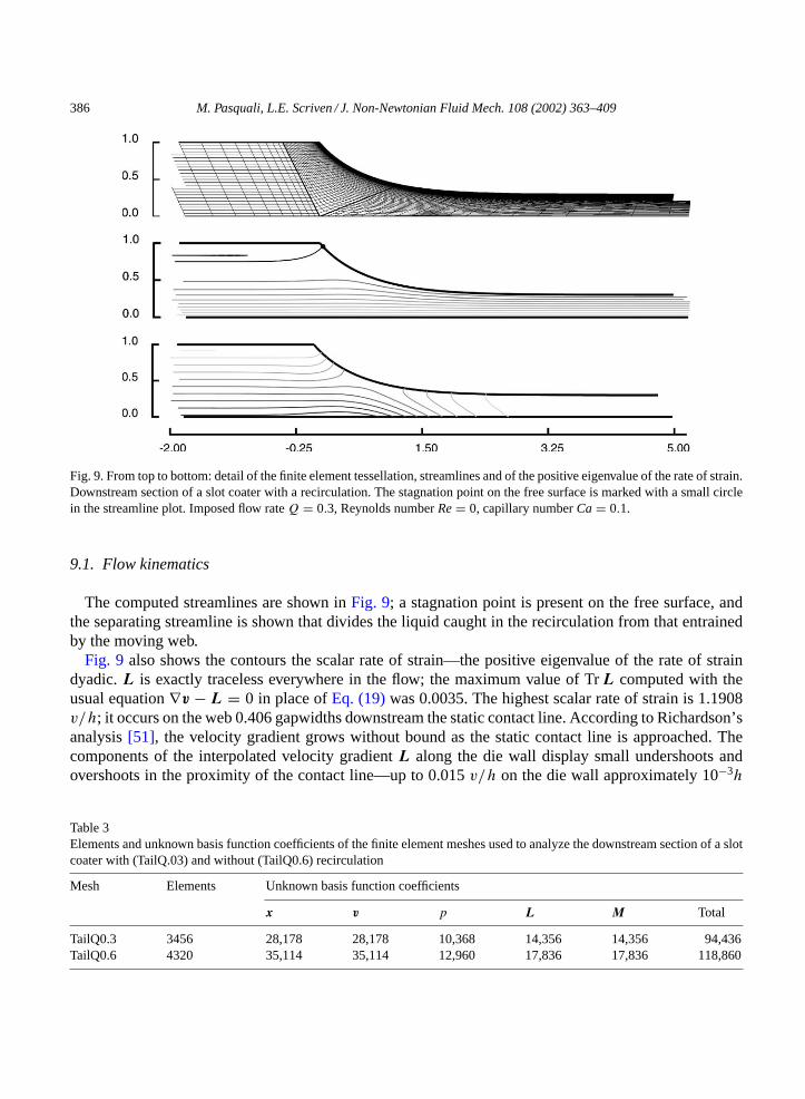
Fig. 9. From top to bottom: detail of the finite element tessellation, streamlines and of the positive eigenvalue of the rate of strain.Downstream section of a slot coater with a recirculation. The stagnation point on the free surface is marked with a small circlein the streamline plot. Imposed flow rateQ = 0.3, Reynolds numberRe= 0, capillary numberCa = 0.1.
9.1. Flow kinematics
The computed streamlines are shown inFig. 9; a stagnation point is present on the free surface, andthe separating streamline is shown that divides the liquid caught in the recirculation from that entrainedby the moving web.
Fig. 9 also shows the contours the scalar rate of strain—the positive eigenvalue of the rate of straindyadic.L is exactly traceless everywhere in the flow; the maximum value of TrL computed with theusual equation∇v − L = 0 in place ofEq. (19)was 0.0035. The highest scalar rate of strain is 1.1908v/h; it occurs on the web 0.406 gapwidths downstream the static contact line. According to Richardson’sanalysis[51], the velocity gradient grows without bound as the static contact line is approached. Thecomponents of the interpolated velocity gradientL along the die wall display small undershoots andovershoots in the proximity of the contact line—up to 0.015v/h on the die wall approximately 10−3h
Table 3Elements and unknown basis function coefficients of the finite element meshes used to analyze the downstream section of a slotcoater with (TailQ.03) and without (TailQ0.6) recirculation
Mesh Elements Unknown basis function coefficients
x v p L M Total
TailQ0.3 3456 28,178 28,178 10,368 14,356 14,356 94,436TailQ0.6 4320 35,114 35,114 12,960 17,836 17,836 118,860
M. Pasquali, L.E. Scriven / J. Non-Newtonian Fluid Mech. 108 (2002) 363–409 387
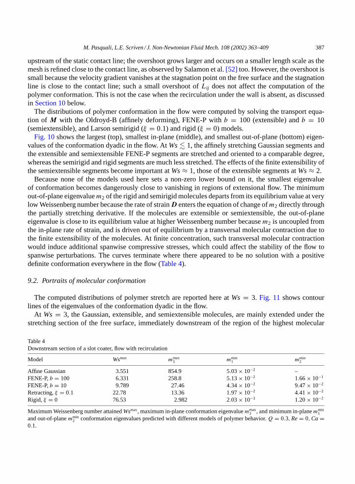
upstream of the static contact line; the overshoot grows larger and occurs on a smaller length scale as themesh is refined close to the contact line, as observed by Salamon et al.[52] too. However, the overshoot issmall because the velocity gradient vanishes at the stagnation point on the free surface and the stagnationline is close to the contact line; such a small overshoot ofLij does not affect the computation of thepolymer conformation. This is not the case when the recirculation under the wall is absent, as discussedin Section 10below.
The distributions of polymer conformation in the flow were computed by solving the transport equa-tion of M with the Oldroyd-B (affinely deforming), FENE-P withb = 100 (extensible) andb = 10(semiextensible), and Larson semirigid (ξ = 0.1) and rigid (ξ = 0) models.
Fig. 10shows the largest (top), smallest in-plane (middle), and smallest out-of-plane (bottom) eigen-values of the conformation dyadic in the flow. AtWs 1, the affinely stretching Gaussian segments andthe extensible and semiextensible FENE-P segments are stretched and oriented to a comparable degree,whereas the semirigid and rigid segments are much less stretched. The effects of the finite extensibility ofthe semiextensible segments become important atWs≈ 1, those of the extensible segments atWs≈ 2.
Because none of the models used here sets a non-zero lower bound on it, the smallest eigenvalueof conformation becomes dangerously close to vanishing in regions of extensional flow. The minimumout-of-plane eigenvaluem2 of the rigid and semirigid molecules departs from its equilibrium value at verylow Weissenberg number because the rate of strainD enters the equation of change ofm2 directly throughthe partially stretching derivative. If the molecules are extensible or semiextensible, the out-of-planeeigenvalue is close to its equilibrium value at higher Weissenberg number becausem2 is uncoupled fromthe in-plane rate of strain, and is driven out of equilibrium by a transversal molecular contraction due tothe finite extensibility of the molecules. At finite concentration, such transversal molecular contractionwould induce additional spanwise compressive stresses, which could affect the stability of the flow tospanwise perturbations. The curves terminate where there appeared to be no solution with a positivedefinite conformation everywhere in the flow (Table 4).
9.2. Portraits of molecular conformation
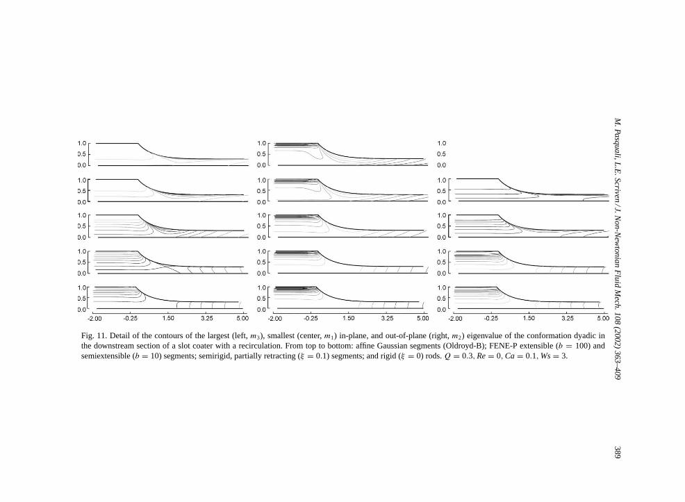
The computed distributions of polymer stretch are reported here atWs = 3. Fig. 11shows contourlines of the eigenvalues of the conformation dyadic in the flow.
At Ws = 3, the Gaussian, extensible, and semiextensible molecules, are mainly extended under thestretching section of the free surface, immediately downstream of the region of the highest molecular
Table 4Downstream section of a slot coater, flow with recirculation
Model Wsmax mmax3 mmin
1 mmin2
Affine Gaussian 3.551 854.9 5.03× 10⁻² –FENE-P,b = 100 6.331 258.8 5.13× 10⁻² 1.66× 10⁻¹
FENE-P,b = 10 9.789 27.46 4.34× 10⁻² 9.47× 10⁻²
Retracting,ξ = 0.1 22.78 13.36 1.97× 10⁻² 4.41× 10⁻²
Rigid, ξ = 0 76.53 2.982 2.03× 10⁻³ 1.20× 10⁻²
Maximum Weissenberg number attainedWsmax, maximum in-plane conformation eigenvaluemmax3 , and minimum in-planemmin
1
and out-of-planemmin2 conformation eigenvalues predicted with different models of polymer behavior.Q = 0.3,Re= 0,Ca =
0.1.
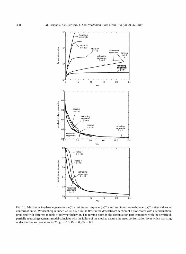
388 M. Pasquali, L.E. Scriven / J. Non-Newtonian Fluid Mech. 108 (2002) 363–409
Fig. 10. Maximum in-plane eigenvalue (mmax3 ), minimum in-plane (mmin
1 ) and minimum out-of-plane (mmin2 ) eigenvalues of
conformation vs. Weissenberg numberWs≡ λv/h in the flow in the downstream section of a slot coater with a recirculation,predicted with different models of polymer behavior. The turning point in the continuation path computed with the semirigid,partially retracting segments model coincides with the failure of the mesh to capture the steep conformation layer which is arisingunder the free surface atWs≈ 20.Q = 0.3,Re= 0,Ca = 0.1.
M.P
asq
ua
li,L.E
.Scrive
n/J.N
on
-New
ton
ian
Flu
idM
ech
.10
8(2
00
2)
36
3–
40
9389
Fig. 11. Detail of the contours of the largest (left,m3), smallest (center,m1) in-plane, and out-of-plane (right,m2) eigenvalue of the conformation dyadic inthe downstream section of a slot coater with a recirculation. From top to bottom: affine Gaussian segments (Oldroyd-B); FENE-P extensible (b = 100) andsemiextensible (b = 10) segments; semirigid, partially retracting (ξ = 0.1) segments; and rigid (ξ = 0) rods.Q = 0.3,Re= 0,Ca = 0.1,Ws= 3.
390 M. Pasquali, L.E. Scriven / J. Non-Newtonian Fluid Mech. 108 (2002) 363–409
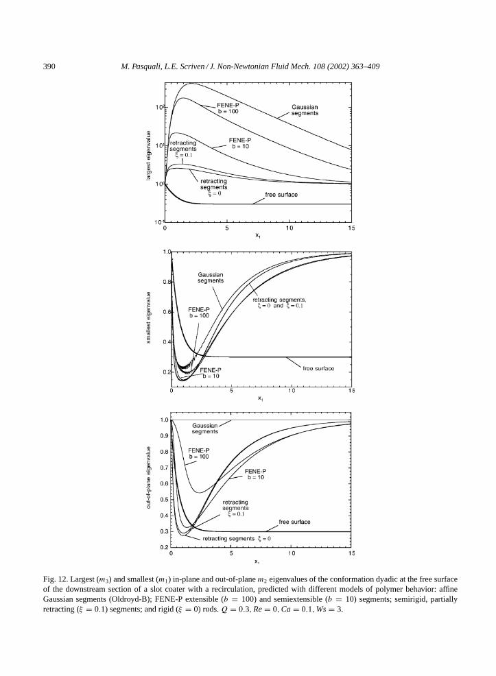
Fig. 12. Largest (m3) and smallest (m1) in-plane and out-of-planem2 eigenvalues of the conformation dyadic at the free surfaceof the downstream section of a slot coater with a recirculation, predicted with different models of polymer behavior: affineGaussian segments (Oldroyd-B); FENE-P extensible (b = 100) and semiextensible (b = 10) segments; semirigid, partiallyretracting (ξ = 0.1) segments; and rigid (ξ = 0) rods.Q = 0.3,Re= 0,Ca = 0.1,Ws= 3.
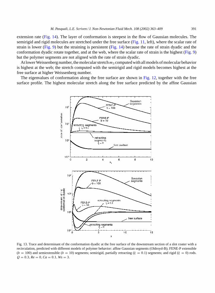
M. Pasquali, L.E. Scriven / J. Non-Newtonian Fluid Mech. 108 (2002) 363–409 391
extension rate (Fig. 14). The layer of conformation is steepest in the flow of Gaussian molecules. Thesemirigid and rigid molecules are stretched under the free surface (Fig. 11, left), where the scalar rate ofstrain is lower (Fig. 9) but the straining is persistent (Fig. 14) because the rate of strain dyadic and theconformation dyadic rotate together, and at the web, where the scalar rate of strain is the highest (Fig. 9)but the polymer segments are not aligned with the rate of strain dyadic.
At lower Weissenberg number, the molecular stretchm3 computed with all models of molecular behavioris highest at the web; the stretch computed with the semirigid and rigid models becomes highest at thefree surface at higher Weissenberg number.
The eigenvalues of conformation along the free surface are shown inFig. 12, together with the freesurface profile. The highest molecular stretch along the free surface predicted by the affine Gaussian
Fig. 13. Trace and determinant of the conformation dyadic at the free surface of the downstream section of a slot coater with arecirculation, predicted with different models of polymer behavior: affine Gaussian segments (Oldroyd-B); FENE-P extensible(b = 100) and semiextensible (b = 10) segments; semirigid, partially retracting (ξ = 0.1) segments; and rigid (ξ = 0) rods.Q = 0.3,Re= 0,Ca = 0.1,Ws= 3.
392 M. Pasquali, L.E. Scriven / J. Non-Newtonian Fluid Mech. 108 (2002) 363–409
segments model is over 100 times larger than that predicted by the rigid rod model. The behavior of thesmallest eigenvalue parallels that of the largest eigenvalue, although it is more difficult to capture the valueof the smallest eigenvalue than it is to approximate the value of the largest eigenvalue of conformation(see[9] for details).
Fig. 13 shows the trace and the determinant of the conformation dyadic along the free surface.If the molecules are extensible or semiextensible, the trace of the conformation is dominated by itslargest eigenvalue and parallels closely its trend. As expected, the trace of the conformation dyadicis constant everywhere if the molecules are rigid. The determinant of the conformation dyadic ofthe affine Gaussian segments grows steadily on the free surface. If the molecules are finitely exten-sible a dip appears in the profiles of detM, although the flowing molecules are effectively largerthan at equilibrium (detM ≥ 1) under the free surface in this case. Conversely, the semirigid andrigid molecules are effectively smaller during the flow because they orient without stretchingappreciably.
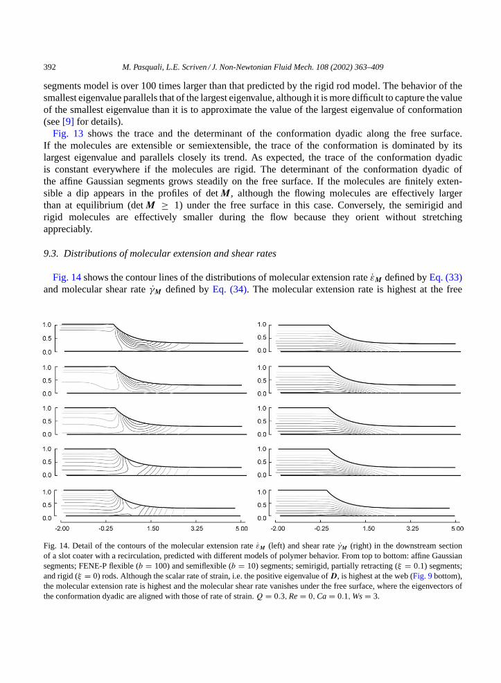
9.3. Distributions of molecular extension and shear rates
Fig. 14shows the contour lines of the distributions of molecular extension rateεM defined byEq. (33)and molecular shear rateγM defined byEq. (34). The molecular extension rate is highest at the free
Fig. 14. Detail of the contours of the molecular extension rateεM (left) and shear rateγM (right) in the downstream sectionof a slot coater with a recirculation, predicted with different models of polymer behavior. From top to bottom: affine Gaussiansegments; FENE-P flexible (b = 100) and semiflexible (b = 10) segments; semirigid, partially retracting (ξ = 0.1) segments;and rigid (ξ = 0) rods. Although the scalar rate of strain, i.e. the positive eigenvalue ofD, is highest at the web (Fig. 9bottom),the molecular extension rate is highest and the molecular shear rate vanishes under the free surface, where the eigenvectors ofthe conformation dyadic are aligned with those of rate of strain.Q = 0.3,Re= 0,Ca = 0.1,Ws= 3.
M. Pasquali, L.E. Scriven / J. Non-Newtonian Fluid Mech. 108 (2002) 363–409 393
surface even though the rate of strain is lower there than at the web (Fig. 9). At Ws= 3, the extensionalcharacter of the flow is stronger in the flows of the extensible and semiextensible molecules than in theflows of the semirigid molecules; overall, the predictions of flow type computed with the different modelsof polymer behavior are very similar.
The distributions of molecular stretch and molecular extension and shear rates show that at low Weis-senberg number the molecules stretch predominantly near the web under the accelerating free sur-face (bottom ofFig. 14) where the rate of strain is highest (bottom ofFig. 9), even though the flowis dominated by shear there (Fig. 14, right). At high Weissenberg number, the molecules stretch un-der the free surface (top ofFig. 11), where the rate of strain is lower than in the web region, butthe straining is persistent (Fig. 14, left). The transition from mild stretching induced by the shearflow at the web to the strong stretching induced by the extensional flow under the accelerating freesurface occurs at lower Weissenberg number for flexible molecules, and at higherWs for the rigidones.
10. Premetered slot coating flow without recirculation, infinitely dilute solutions
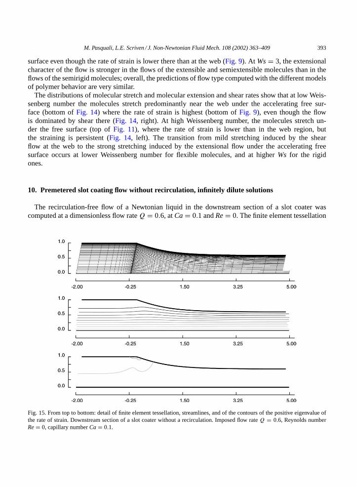
The recirculation-free flow of a Newtonian liquid in the downstream section of a slot coater wascomputed at a dimensionless flow rateQ = 0.6, atCa = 0.1 andRe= 0. The finite element tessellation
Fig. 15. From top to bottom: detail of finite element tessellation, streamlines, and of the contours of the positive eigenvalue ofthe rate of strain. Downstream section of a slot coater without a recirculation. Imposed flow rateQ = 0.6, Reynolds numberRe= 0, capillary numberCa = 0.1.
394 M. Pasquali, L.E. Scriven / J. Non-Newtonian Fluid Mech. 108 (2002) 363–409
had 4320 elements strongly concentrated near the static contact line to capture the high velocity gradientand the layer of conformation that arises there (Figs. 8 and 15andTable 3).
10.1. Flow kinematics
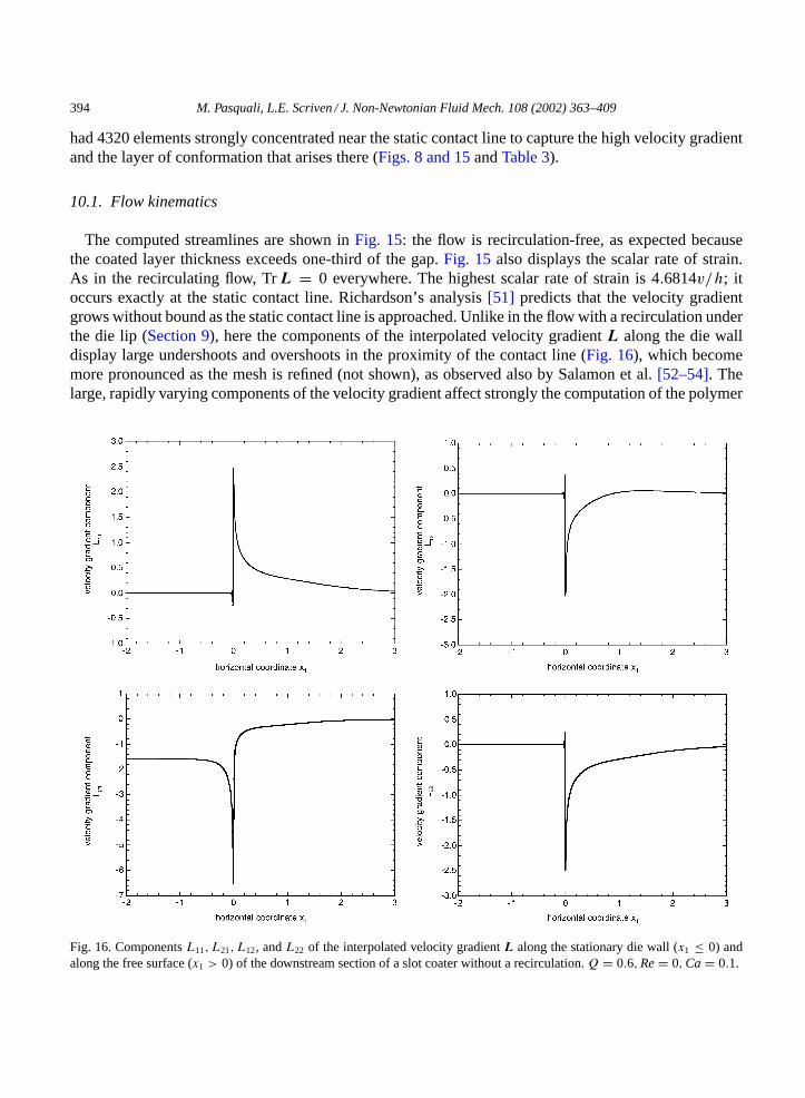
The computed streamlines are shown inFig. 15: the flow is recirculation-free, as expected becausethe coated layer thickness exceeds one-third of the gap.Fig. 15also displays the scalar rate of strain.As in the recirculating flow, TrL = 0 everywhere. The highest scalar rate of strain is 4.6814v/h; itoccurs exactly at the static contact line. Richardson’s analysis[51] predicts that the velocity gradientgrows without bound as the static contact line is approached. Unlike in the flow with a recirculation underthe die lip (Section 9), here the components of the interpolated velocity gradientL along the die walldisplay large undershoots and overshoots in the proximity of the contact line (Fig. 16), which becomemore pronounced as the mesh is refined (not shown), as observed also by Salamon et al.[52–54]. Thelarge, rapidly varying components of the velocity gradient affect strongly the computation of the polymer
Fig. 16. ComponentsL11, L21, L12, andL22 of the interpolated velocity gradientL along the stationary die wall (x1 ≤ 0) andalong the free surface (x1 > 0) of the downstream section of a slot coater without a recirculation.Q = 0.6,Re= 0,Ca = 0.1.
M. Pasquali, L.E. Scriven / J. Non-Newtonian Fluid Mech. 108 (2002) 363–409 395
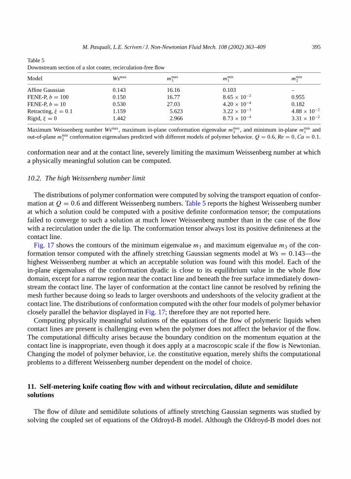
Table 5Downstream section of a slot coater, recirculation-free flow
Model Wsmax mmax3 mmin
1 mmin2
Affine Gaussian 0.143 16.16 0.103 –FENE-P,b = 100 0.150 16.77 8.65× 10⁻² 0.955FENE-P,b = 10 0.530 27.03 4.20× 10⁻⁴ 0.182Retracting,ξ = 0.1 1.159 5.623 3.22× 10⁻³ 4.88× 10⁻²
Rigid, ξ = 0 1.442 2.966 8.73× 10⁻⁴ 3.31× 10⁻²
Maximum Weissenberg numberWsmax, maximum in-plane conformation eigenvaluemmax3 , and minimum in-planemmin
1 andout-of-planemmin
2 conformation eigenvalues predicted with different models of polymer behavior.Q = 0.6,Re= 0,Ca = 0.1.
conformation near and at the contact line, severely limiting the maximum Weissenberg number at whicha physically meaningful solution can be computed.
10.2. The high Weissenberg number limit
The distributions of polymer conformation were computed by solving the transport equation of confor-mation atQ = 0.6 and different Weissenberg numbers.Table 5reports the highest Weissenberg numberat which a solution could be computed with a positive definite conformation tensor; the computationsfailed to converge to such a solution at much lower Weissenberg number than in the case of the flowwith a recirculation under the die lip. The conformation tensor always lost its positive definiteness at thecontact line.
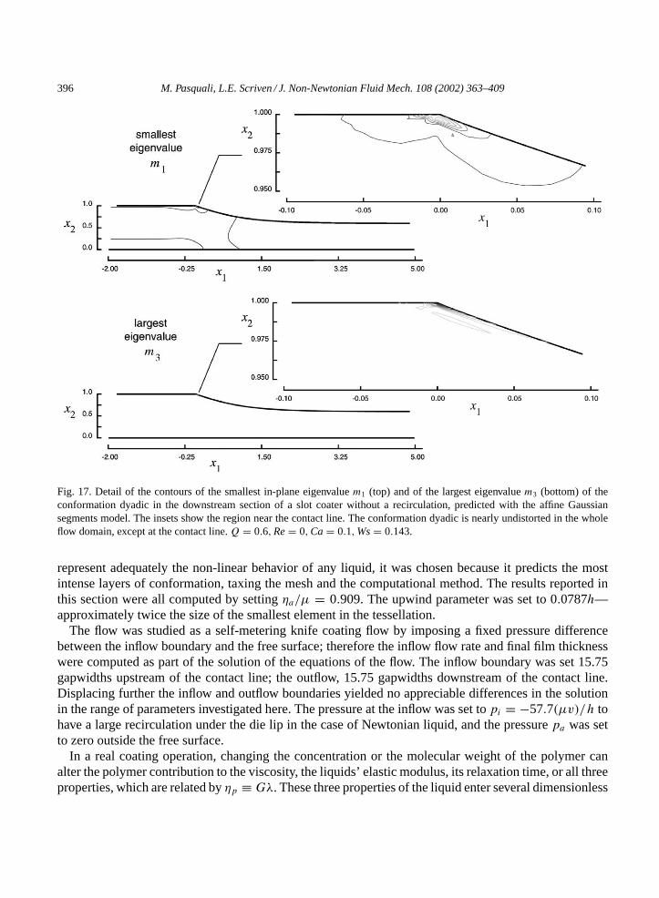
Fig. 17shows the contours of the minimum eigenvaluem1 and maximum eigenvaluem3 of the con-formation tensor computed with the affinely stretching Gaussian segments model atWs= 0.143—thehighest Weissenberg number at which an acceptable solution was found with this model. Each of thein-plane eigenvalues of the conformation dyadic is close to its equilibrium value in the whole flowdomain, except for a narrow region near the contact line and beneath the free surface immediately down-stream the contact line. The layer of conformation at the contact line cannot be resolved by refining themesh further because doing so leads to larger overshoots and undershoots of the velocity gradient at thecontact line. The distributions of conformation computed with the other four models of polymer behaviorclosely parallel the behavior displayed inFig. 17; therefore they are not reported here.
Computing physically meaningful solutions of the equations of the flow of polymeric liquids whencontact lines are present is challenging even when the polymer does not affect the behavior of the flow.The computational difficulty arises because the boundary condition on the momentum equation at thecontact line is inappropriate, even though it does apply at a macroscopic scale if the flow is Newtonian.Changing the model of polymer behavior, i.e. the constitutive equation, merely shifts the computationalproblems to a different Weissenberg number dependent on the model of choice.
11. Self-metering knife coating flow with and without recirculation, dilute and semidilutesolutions
The flow of dilute and semidilute solutions of affinely stretching Gaussian segments was studied bysolving the coupled set of equations of the Oldroyd-B model. Although the Oldroyd-B model does not
396 M. Pasquali, L.E. Scriven / J. Non-Newtonian Fluid Mech. 108 (2002) 363–409
Fig. 17. Detail of the contours of the smallest in-plane eigenvaluem1 (top) and of the largest eigenvaluem3 (bottom) of theconformation dyadic in the downstream section of a slot coater without a recirculation, predicted with the affine Gaussiansegments model. The insets show the region near the contact line. The conformation dyadic is nearly undistorted in the wholeflow domain, except at the contact line.Q = 0.6,Re= 0,Ca = 0.1,Ws= 0.143.
represent adequately the non-linear behavior of any liquid, it was chosen because it predicts the mostintense layers of conformation, taxing the mesh and the computational method. The results reported inthis section were all computed by settingηa/µ = 0.909. The upwind parameter was set to 0.0787h—approximately twice the size of the smallest element in the tessellation.
The flow was studied as a self-metering knife coating flow by imposing a fixed pressure differencebetween the inflow boundary and the free surface; therefore the inflow flow rate and final film thicknesswere computed as part of the solution of the equations of the flow. The inflow boundary was set 15.75gapwidths upstream of the contact line; the outflow, 15.75 gapwidths downstream of the contact line.Displacing further the inflow and outflow boundaries yielded no appreciable differences in the solutionin the range of parameters investigated here. The pressure at the inflow was set topi = −57.7(µv)/h tohave a large recirculation under the die lip in the case of Newtonian liquid, and the pressurepa was setto zero outside the free surface.
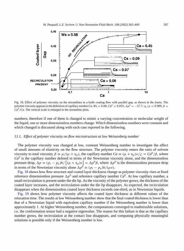
In a real coating operation, changing the concentration or the molecular weight of the polymer canalter the polymer contribution to the viscosity, the liquids’ elastic modulus, its relaxation time, or all threeproperties, which are related byηp ≡ Gλ. These three properties of the liquid enter several dimensionless
M. Pasquali, L.E. Scriven / J. Non-Newtonian Fluid Mech. 108 (2002) 363–409 397
Fig. 18. Effect of polymer viscosity on the streamlines in a knife coating flow with parallel gap, as shown in the insets. Thepolymer viscosity appears in the definition of capillary numberCa.Ws= 0.08; Ca0 = 0.055;@p0 = −57.7; ηa/µ = 0.909;β =Ca0/Ca. The vertical scale is enlarged in the streamline plots.
numbers; therefore if one of them is changed to mimic a varying concentration or molecular weight ofthe liquid, one or more dimensionless numbers change. Which dimensionless numbers were constant andwhich changed is discussed along with each case reported in the following.
11.1. Effect of polymer viscosity on flow microstructure at low Weissenberg number
The polymer viscosity was changed at low, constant Weissenberg number to investigate the effectof small amounts of elasticity on the flow structure. The polymer viscosity enters the ratio of solventviscosity to total viscosityβ ≡ µ/(µ+ ηp), the capillary numberCa ≡ (µ+ ηp)v/ς = Ca0/β, whereCa0 is the capillary number defined in terms of the Newtonian viscosity alone, and the dimensionlesspressure drop,@p ≡ (pi − pa)h/
[(µ+ ηp)v
] = @p0β, where@p0 is the dimensionless pressure dropin terms of the Newtonian viscosity alone@p0 ≡ (pi − pa)h/(µv).
Fig. 18shows how flow structure and coated layer thickness change as polymer viscosity rises at fixedreference dimensionless pressure@p0 and reference capillary numberCa0. At low capillary number, asmall recirculation is present under the die lip. As the viscosity of the polymer grows, the thickness of thecoated layer increases, and the recirculation under the die lip disappears. As expected, the recirculationdisappears when the dimensionless coated layer thickness exceeds one-third, as in Newtonian liquids.
Fig. 19 shows how polymer viscosity affects the coated layer thickness at different values of therelaxation time. The results at low Weissenberg number show that the final coated thickness is lower thanthat of a Newtonian liquid with equivalent capillary number if the Weissenberg number is lower thanapproximately 1. At higher Weissenberg number, the computations converged to inadmissible solutions,i.e. the conformation tensor had a negative eigenvalue. The reason for this failure is that as the capillarynumber grows, the recirculation at the contact line disappears, and computing physically meaningfulsolutions is possible only if the Weissenberg number is low.
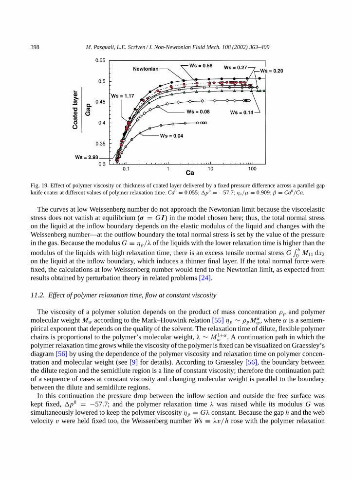
398 M. Pasquali, L.E. Scriven / J. Non-Newtonian Fluid Mech. 108 (2002) 363–409
Fig. 19. Effect of polymer viscosity on thickness of coated layer delivered by a fixed pressure difference across a parallel gapknife coater at different values of polymer relaxation time.Ca0 = 0.055;@p0 = −57.7; ηa/µ = 0.909;β = Ca0/Ca.
The curves at low Weissenberg number do not approach the Newtonian limit because the viscoelasticstress does not vanish at equilibrium (σ = GI ) in the model chosen here; thus, the total normal stresson the liquid at the inflow boundary depends on the elastic modulus of the liquid and changes with theWeissenberg number—at the outflow boundary the total normal stress is set by the value of the pressurein the gas. Because the modulusG ≡ ηp/λ of the liquids with the lower relaxation time is higher than themodulus of the liquids with high relaxation time, there is an excess tensile normal stressG
∫ h0 M11 dx2
on the liquid at the inflow boundary, which induces a thinner final layer. If the total normal force werefixed, the calculations at low Weissenberg number would tend to the Newtonian limit, as expected fromresults obtained by perturbation theory in related problems[24].
11.2. Effect of polymer relaxation time, flow at constant viscosity
The viscosity of a polymer solution depends on the product of mass concentrationρp and polymermolecular weightMw according to the Mark–Houwink relation[55] ηp ∼ ρpMα
w, whereα is a semiem-pirical exponent that depends on the quality of the solvent. The relaxation time of dilute, flexible polymerchains is proportional to the polymer’s molecular weight,λ ∼ M1+α
w . A continuation path in which thepolymer relaxation time grows while the viscosity of the polymer is fixed can be visualized on Graessley’sdiagram[56] by using the dependence of the polymer viscosity and relaxation time on polymer concen-tration and molecular weight (see[9] for details). According to Graessley[56], the boundary betweenthe dilute region and the semidilute region is a line of constant viscosity; therefore the continuation pathof a sequence of cases at constant viscosity and changing molecular weight is parallel to the boundarybetween the dilute and semidilute regions.
In this continuation the pressure drop between the inflow section and outside the free surface waskept fixed,@p0 = −57.7; and the polymer relaxation timeλ was raised while its modulusG wassimultaneously lowered to keep the polymer viscosityηp = Gλ constant. Because the gaph and the webvelocity v were held fixed too, the Weissenberg numberWs≡ λv/h rose with the polymer relaxation
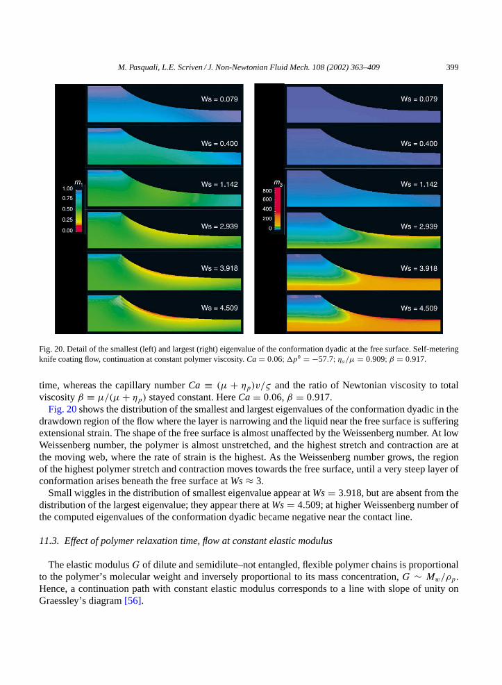
M. Pasquali, L.E. Scriven / J. Non-Newtonian Fluid Mech. 108 (2002) 363–409 399
Fig. 20. Detail of the smallest (left) and largest (right) eigenvalue of the conformation dyadic at the free surface. Self-meteringknife coating flow, continuation at constant polymer viscosity.Ca = 0.06;@p0 = −57.7; ηa/µ = 0.909;β = 0.917.
time, whereas the capillary numberCa ≡ (µ + ηp)v/ς and the ratio of Newtonian viscosity to totalviscosityβ ≡ µ/(µ+ ηp) stayed constant. HereCa = 0.06,β = 0.917.
Fig. 20shows the distribution of the smallest and largest eigenvalues of the conformation dyadic in thedrawdown region of the flow where the layer is narrowing and the liquid near the free surface is sufferingextensional strain. The shape of the free surface is almost unaffected by the Weissenberg number. At lowWeissenberg number, the polymer is almost unstretched, and the highest stretch and contraction are atthe moving web, where the rate of strain is the highest. As the Weissenberg number grows, the regionof the highest polymer stretch and contraction moves towards the free surface, until a very steep layer ofconformation arises beneath the free surface atWs≈ 3.
Small wiggles in the distribution of smallest eigenvalue appear atWs= 3.918, but are absent from thedistribution of the largest eigenvalue; they appear there atWs= 4.509; at higher Weissenberg number ofthe computed eigenvalues of the conformation dyadic became negative near the contact line.
11.3. Effect of polymer relaxation time, flow at constant elastic modulus
The elastic modulusG of dilute and semidilute–not entangled, flexible polymer chains is proportionalto the polymer’s molecular weight and inversely proportional to its mass concentration,G ∼ Mw/ρp.Hence, a continuation path with constant elastic modulus corresponds to a line with slope of unity onGraessley’s diagram[56].
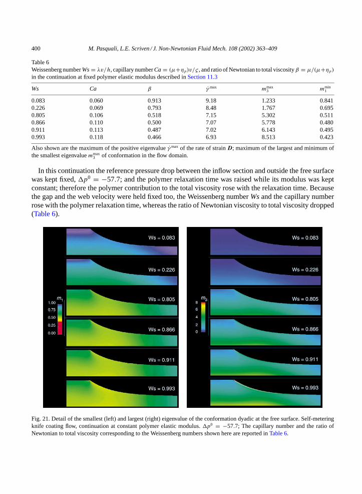
400 M. Pasquali, L.E. Scriven / J. Non-Newtonian Fluid Mech. 108 (2002) 363–409
Table 6Weissenberg numberWs= λv/h, capillary numberCa = (µ+ηp)v/ς , and ratio of Newtonian to total viscosityβ = µ/(µ+ηp)in the continuation at fixed polymer elastic modulus described inSection 11.3
Ws Ca β γmax mmax3 mmin
1
0.083 0.060 0.913 9.18 1.233 0.8410.226 0.069 0.793 8.48 1.767 0.6950.805 0.106 0.518 7.15 5.302 0.5110.866 0.110 0.500 7.07 5.778 0.4800.911 0.113 0.487 7.02 6.143 0.4950.993 0.118 0.466 6.93 8.513 0.423
Also shown are the maximum of the positive eigenvalueγmax of the rate of strainD; maximum of the largest and minimum ofthe smallest eigenvaluemmax
3 of conformation in the flow domain.
In this continuation the reference pressure drop between the inflow section and outside the free surfacewas kept fixed,@p0 = −57.7; and the polymer relaxation time was raised while its modulus was keptconstant; therefore the polymer contribution to the total viscosity rose with the relaxation time. Becausethe gap and the web velocity were held fixed too, the Weissenberg numberWsand the capillary numberrose with the polymer relaxation time, whereas the ratio of Newtonian viscosity to total viscosity dropped(Table 6).
Fig. 21. Detail of the smallest (left) and largest (right) eigenvalue of the conformation dyadic at the free surface. Self-meteringknife coating flow, continuation at constant polymer elastic modulus.@p0 = −57.7; The capillary number and the ratio ofNewtonian to total viscosity corresponding to the Weissenberg numbers shown here are reported inTable 6.
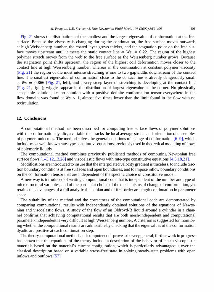
M. Pasquali, L.E. Scriven / J. Non-Newtonian Fluid Mech. 108 (2002) 363–409 401
Fig. 21shows the distributions of the smallest and the largest eigenvalue of conformation at the freesurface. Because the viscosity is changing during the continuation, the free surface moves outwardsat high Weissenberg number, the coated layer grows thicker, and the stagnation point on the free sur-face moves upstream until it meets the static contact line atWs ≈ 0.22. The region of the highestpolymer stretch moves from the web to the free surface as the Weissenberg number grows. Becausethe stagnation point shifts upstream, the region of the highest coil deformation moves closer to thecontact line at high Weissenberg number, whereas in the continuation at constant polymer viscosity(Fig. 21) the region of the most intense stretching is one to two gapwidths downstream of the contactline. The smallest eigenvalue of conformation close to the contact line is already dangerously smallat Ws = 0.866 (Fig. 21, left), and a very steep layer of stretching is developing at the contact line(Fig. 21, right); wiggles appear in the distribution of largest eigenvalue at the corner. No physicallyacceptable solution, i.e. no solution with a positive definite conformation tensor everywhere in theflow domain, was found atWs> 1, almost five times lower than the limit found in the flow with norecirculation.
12. Conclusions
A computational method has been described for computing free surface flows of polymer solutionswith the conformation dyadic, a variable that tracks the local average stretch and orientation of ensemblesof polymer molecules. The method solves the general equations of change of conformation[6–9], whichinclude most well-known rate-type constitutive equations previously used in theoretical modeling of flowsof polymeric liquids.
The computational method combines previously published methods of computing Newtonian freesurface flows[1–3,12,13,28]and viscoelastic flows with rate-type constitutive equations[4,5,18,21].
Modifications are introduced to insure that the interpolated velocity gradient is traceless, to include trac-tion boundary conditions at free surfaces and open boundaries, and to impose inflow boundary conditionson the conformation tensor that are independent of the specific choice of constitutive model.
A new way is introduced of writing computational code that is independent of the number and type ofmicrostructural variables, and of the particular choice of the mechanisms of change of conformation, yetretains the advantages of a full analytical Jacobian and of first-order arclength continuation in parameterspace.
The suitability of the method and the correctness of the computational code are demonstrated bycomparing computational results with independently obtained solutions of the equations of Newto-nian and viscoelastic flows. A study of the flow of an Oldroyd-B liquid around a cylinder in a chan-nel confirms that achieving computational results that are both mesh-independent and computationalparameter-independent is very difficult at high Weissenberg number. A criterion is suggested for monitor-ing whether the computational results are admissible by checking that the eigenvalues of the conformationdyadic are positive at each continuation step.
The theory, computational method, and computer code prove to be very general; further work in progresshas shown that the equations of the theory include a description of the behavior of elasto-viscoplasticmaterials based on the material’s current configuration, which is particularly advantageous over theclassical description based on a variable stress-free state in solving steady-state problems with openinflows and outflows[57].
402 M. Pasquali, L.E. Scriven / J. Non-Newtonian Fluid Mech. 108 (2002) 363–409
The computational method was used to analyze the premetered flow of infinitely dilute solutions ofpolymer of varying degree of stiffness under the downstream section of a slot coater was analyzed bothwith and without a recirculation under the die wall, as well as the self-metering pressure-driven flow ofdilute and semidilute solutions—represented by the Oldroyd-B model—beneath the downstream sectionof a knife coater, where the transition between recirculating and recirculation-free flow was investigated.
The solutions of the governing equations show that if a recirculation is present, the approximate valueof the velocity gradient field is low in the small region between the static contact line and the stagnationpoint on the free surface even when the mesh is refined, although a mathematical singularity is presentat the contact line. Small overshoots and undershoots of the velocity gradient are present, which do notprevent the solution of the equations of the flow at high Weissenberg number (Ws 3).
Once the recirculation is absent, the singularity at the contact line strongly affects locally the velocitygradient, which in turn affects the value of the molecular conformation dyadic there; the solutions atmoderate Weissenberg number (Ws ≈ 0.15) are unacceptable because one of the eigenvalues of theconformation dyadic is negative at the contact line, irrespective of the type of polymer model and regardlessof whether the polymer is affecting the flow or not.
The equation set yields unacceptable solutions near the contact line because the boundary conditionsthere (no slip on the solid wall, no shear stress on the free surface) are inappropriate; these boundaryconditions hold on a macroscopic scale if the flow is Newtonian. More research is needed on appropriateboundary conditions at contact lines in the flow of polymeric liquids, possibly including in the theorythe migration of polymer molecules away from regions of highly stretched conformation (or high elasticstress).
When a recirculation was present under the die, the solution of the equations at high Weissenbergnumber lost meaning because the smallest eigenvalue of conformation became negative. None of themodels of polymer dynamics known to the authors sets a non-zero lower bound on the eigenvalues ofconformation. If an eigenvaluemi associated with an eigenvectormi vanishes, then all polymer seg-ments must be oriented perpendicular tomi . Whether such a perfect alignment can be approached, orif a non-zero lower bound should exist on the eigenvalues of the conformation dyadic, is simply notknown.
New indicators of molecular extensional rate and molecular shear rate have been introduced. Theyare independent of frame of reference and coordinate systems, and they are rooted in the molecularinterpretation of the conformation dyadic as representative of the local average state of stretch andorientation of the molecules in the flow. These flow-type indicators indicate that the stretching at highWeissenberg number occurs under the free surface, where the straining is persistent and the molecularconformation dyadic is aligned with the rate of strain, i.e. the flow is extensional, even though the strainrate is lower there than at the web. At low Weissenberg number, the molecules stretch little, and do sonear the web in the region of the highest strain rate.
Some models of polymer behavior used here predict a contraction of the conformation tensor in thespanwise direction in a two-dimensional flow which induce spanwise compressive elastic stresses thatmay effect the stability of the flow. If the molecules are extensible or semiextensible, this contractionoccurs after the molecules stretch in the in-plane direction, and is a consequence of their finite extensi-bility. If they are rigid, the contraction occurs at lower Weissenberg number because it is caused by flowrather than molecular relaxation. Because current experimental evidence is inconclusive[9,58,59], it willtake further experiments to answer the question of whether or not the molecular conformation tensorcontracts.
M. Pasquali, L.E. Scriven / J. Non-Newtonian Fluid Mech. 108 (2002) 363–409 403
Acknowledgements
Thanks are due to Prof. Marcio S. Carvalho for useful discussions on Newtonian free surface flows. Thisresearch was supported by NSF and industrial sponsors through the Center for Interfacial Engineeringand by generous grants of computing time by the University of Minnesota Supercomputing Institute.
Appendix A. Formulae of the analytical Jacobian
The derivatives of the residual equations with respect to the unknown basis function coefficients arereported here together with a number of useful recurring formulae.
• Derivatives of the Jacobian of the mappingf with respect to position basis functions coefficientsxαj :
∂f
∂xαj= f∇jϕαx (A.1)
• Derivatives of the direct mapping deformation gradientF with respect to position basis functionscoefficientsxαk :
∂Fij
∂xαk= δkj
∂ϕαx
∂ξi(A.2)
• Derivatives of the inverse mapping deformation gradientK with respect to position basis functionscoefficientsxαj :
∂Kki
∂xαj= −Kji∇kϕαx (A.3)
• Derivatives of the gradient of a scalar, vector component, or tensor componentGwith respect to positionbasis functions coefficientsxαj :
∂∇kG∂xαj
= −(∇jG)∇kϕαx (A.4)
• Derivatives of componentai of a vectora with respect to componentaj of the vector itself, withδij asthe Kronecker delta (ij component of the idemfactorI ):
∂ai
∂aj= δij (A.5)
• Derivatives of componentAij of a tensor with respect to componentAkl of the tensor itself:
∂Aij
∂Akl= δikδjl (A.6)
• Derivatives of the invariants of a dyadic with respect to the component of the dyadic itself (not neces-sarily symmetric):
∂IA
∂Aij= δij (A.7)
404 M. Pasquali, L.E. Scriven / J. Non-Newtonian Fluid Mech. 108 (2002) 363–409
∂IIA
∂Aij≡ 1
2
∂
∂Aij
[(Tr A)2 − Tr (A2)
] = IAδij − Aji (A.8)
∂III A
∂Aij= AjkAki − IAAji + IIAδij = III AA
−1ji (A.9)
whereIA ≡ Tr A ≡ I : A, andIII A ≡ detA;• Derivatives of the stressT with respect to position basis functions coefficientsxαj :
∂Tki
∂xαj= −ηa
[(∇j vi)∇kϕαx + (∇j vk)∇iϕαx
](A.10)
• Derivatives of the stressT with respect to velocity basis functions coefficientsvαj :
∂Tki
∂vαj= ηa
(δij∇kϕαv + δjk∇iϕαv
)(A.11)
• Derivatives of the elastic stressσ with respect to conformationM:
∂σli
Mjk= 2
(∂ξ
∂Mjk− ∂ζ
∂Mjk
)M : A
I : MMli − 2
ξ − ζ(I : M)2
A : MMliδjk
+ 2ξ − ζI : M
(AkjMli +Mpq
∂Aqp
∂MjkMli + M : Aδjlδki
)+ 2
∂ζ
∂MjkMlpApi
+ 2ζ
(δjlAki +Mlp
∂Api
∂Mjk
)(A.12)
whereA is the derivative of the free energy with respect to conformation,
A ≡ ∂a
∂M(A.13)
Aij ≡ ∂a
∂Mij= ∂a
∂IM
∂IM
∂Mij+ ∂a
∂IIM
∂IIM
∂Mij+ ∂a
∂III M
∂III M
∂Mij
=(∂a
∂IM+ ∂a
∂IIM
)δij − ∂a
∂IIM
Mji + III M
∂a
∂III M
M−1ji (A.14)
Eqs. (A.1) and (A.14)hold in two- and three-dimensional flows.
A.1. Derivatives of the elliptic mesh generation equation
A.1.1. Derivatives with respect to position basis functions coefficients
∂rx,γi
∂xαj=∫Ω0
(∇kϕαx ∇jψγx DklKlif − ∇kψγx DklKji∇lϕαxf − ∇kψγx DklKli
∂f
∂xαj
)dΩ0
+ boundary terms (A.15)
M. Pasquali, L.E. Scriven / J. Non-Newtonian Fluid Mech. 108 (2002) 363–409 405
A.2. Derivatives of the continuity equation
A.2.1. Derivatives with respect to position basis functions coefficients
∂rc,γ
∂xαj=∫Ω0
ψγc
(∂f
∂xαj∇ · v − f∇j vi∇iϕαx
)dΩ0 (A.16)
A.2.2. Derivatives with respect to velocity basis functions coefficients∂rc,γ
∂vαj=∫Ω0
ψγc ∇jϕαv f dΩ0 (A.17)
A.3. Derivatives of the momentum transport equation
A.3.1. Derivatives with respect to position basis functions coefficients
∂rm,γi
∂xαp=∫Ω0
∂f
∂xαp[ψγmρ(v · ∇vi − ∇iΘ)+ ∇kψγmTki]
+ f[−ψγmρv · ∇ϕαx ∇pvi − ∇pψγm∇kϕαxTki + ∇kψγm
∂Tki
∂xαp
]dΩ0
+ boundary terms (A.18)
A.3.2. Derivatives with respect to velocity basis functions coefficients
∂rm,γi
∂vαj=∫Ω0
[ψγmρ(ϕ
αv ∇j vi + δijv · ∇ϕαv )+ ∇kψγm
∂Tki
∂vαj
]f dΩ0 + boundary terms (A.19)
A.3.3. Derivatives with respect to pressure basis functions coefficients
∂rm,γi
∂pα= −
∫Ω0
∇iψγmϕαpf dΩ0 + boundary terms (A.20)
A.3.4. Derivatives with respect to interpolated velocity gradient basis functions coefficients
∂rm,γi
∂Lαjk=∫Ω0
ϕαL
[(µ− ηa)(∇jψγmδki + ∇kψγmδij )+ ∇lψγm
∂ηa
∂Ljk(∇lvi − Lli + ∇ivl − Lil )
]f dΩ0
+ boundary terms (A.21)
A.3.5. Derivatives with respect to conformation basis functions coefficients
∂rm,γi
∂Mαjk
= −∫Ω0
ϕαM∇lψγm[∂ηa
∂Mjk(∇lvi − Lli + ∇ivl − Lil )+ ∂σli
∂Mjk
]f dΩ0
+ boundary terms (A.22)
406 M. Pasquali, L.E. Scriven / J. Non-Newtonian Fluid Mech. 108 (2002) 363–409
A.4. Derivatives of the velocity gradient interpolation equation
A.4.1. Derivatives with respect to position basis functions coefficients
∂RL,αij
∂xγ
k
=∫Ω0
ψαL
[∂f
∂xαk
(Lij − ∇ivj + 1
Tr I∇ · vδij
)
+ f(
∇iϕγx ∇kvj − 1
Tr I∇pϕγx ∇kvpδij
)]dΩ0 (A.23)
A.4.2. Derivatives with respect to velocity basis functions coefficients
∂RL,αij
∂vγ
k
=∫Ω0
ψαL
(−δjk∇iϕγv + 1
Tr I∇kϕγv δij
)f dΩ0 (A.24)
A.4.3. Derivatives with respect to interpolated velocity gradient basis functions coefficients
∂RL,αij
∂Lγ
kl
=∫Ω0
ψαLδikδjlϕγ
Lf dΩ0 (A.25)
A.5. Derivatives of the conformation transport equation
A.5.1. Derivatives with respect to position basis functions coefficients
∂RM,γij
∂xαk=∫Ω0
[∂f
∂xαkψγ
M + f(∂h
∂xαkv · ∇ϕγM − hv · ∇ϕαx ∇kϕγM
)]
×(
v · ∇Mij + Pij + 1
λSij
)− fψγMv · ∇ϕαx ∇kMij
dΩ0 (A.26)
where
Pij ≡ −2ξD : M
I : MMij − ζ
(MilDlj +DilMlj − 2
D : M
I : MMij
)−MilWlj −WliMlj (A.27)
Sij ≡ g0δij + g1Mij + g2MilMlj (A.28)
A.5.2. Derivatives with respect to velocity basis functions coefficients∂R
M,γij
∂xαk=∫Ω0
[ψγ
Mϕαv ∇kMij + hϕαv ∇kϕγM
(v · ∇Mij + Pij + 1
λSij
)]f dΩ0 (A.29)
A.5.3. Derivatives with respect to interpolated velocity gradient basis functions coefficients
∂RM,γij
∂Lαkl
=∫Ω0
ψγ
MϕαL
[−(ξ − ζ )Mkl +Mlk
I : MMij − 1
2ζ(Mikδjl +Milδkj + δikMlj + δilMkj)
− 1
2(Mikδjl −Milδjk + δilMkj − δikMlj )
]f dΩ0 (A.30)
M. Pasquali, L.E. Scriven / J. Non-Newtonian Fluid Mech. 108 (2002) 363–409 407
A.5.4. Derivatives with respect to conformation basis functions coefficients
∂RM,γij
∂Mαkl
=∫Ω0
ψγ
M
v · ∇ϕαMδikδjl + ϕαM
[−2
(∂ξ
∂Mkl− ∂ζ
∂Mkl
)D : M
I : MMij
− 2(ξ − ζ )(Dkl
I : MMij − D : M
(I : M)2δklMij + D : M
I : Mδikδjl
)
− ∂ζ
∂Mkl(MipDpj +DipMpj)− ζ(δikDlj +Dikδjl )
+ 1
λ
(∂g0
∂Mklδij + ∂g1
∂MklMij + g1δikδjl + ∂g2
∂MklMipMpj + g2(δikMlj +Mikδjl )
)]f dΩ0
(A.31)
References
[1] K.N. Christodoulou, L.E. Scriven, Discretization of free surface flows and other moving boundary problems, J. Comp.Phys. 99 (1992) 39–55.
[2] V.F. deAlmeida, Gas–Liquid Counterflow Through Constricted Passages, Ph.D. thesis, University of Minnesota,Minneapolis, MN, 1995 (Available from UMI, Ann Arbor, MI, order number 9615160).
[3] P.A. Sackinger, P.R. Schunk, R.R. Rao, A Newton–Raphson pseudo-solid domain mapping technique for free and movingboundary problems: a finite element implementation, J. Comp. Phys. 125 (1996) 83–103.
[4] R. Guénette, M. Fortin, A new finite element method for computing viscoelastic flows, J. Non-Newtonian Fluid Mech. 60(1995) 27–52.
[5] M.J. Szady, T.R. Salamon, A.W. Liu, R.C. Armstrong, R.A. Brown, A new mixed finite element method for viscoelasticflows governed by differential constitutive equations, J. Non-Newtonian Fluid Mech. 59 (1995) 215–243.
[6] M. Grmela, P.J. Carreau, Conformation tensor rheological models, J. Non-Newtonian Fluid Mech. 23 (1987) 271–294.[7] A.N. Beris, B.J. Edwards, Thermodynamics of Flowing Systems with Internal Microstructure, 1st ed., Oxford University
Press, Oxford, 1994.[8] R.J.J. Jongschaap, K.H. deHaas, C.A.J. Damen, A generic matrix representation of configuration tensor rheological models,
J. Rheol. 38 (1994) 769–796.[9] M. Pasquali, Polymer Molecules in Free Surface Coating Flows, Ph.D. thesis, University of Minnesota, Minneapolis, MN,
2000 (Available from UMI, Ann Arbor, MI, order number 9963019).[10] S.F. Kistler, L.E. Scriven, Coating flows, in: J.R.A. Pearson, S.M. Richardson (Eds.), Computational Analysis of Polymer
Processing, Applied Science Publishers, London, 1983, pp. 243–299.[11] S.F. Kistler, L.E. Scriven, Coating flow theory by finite element and asymptotic analysis of the Navier–Stokes system, Int.
J. Numer. Methods Fluid. 4 (1984) 207–229.[12] K.N. Christodoulou, Computational Physics of Slide Coating Flow, Ph.D. thesis, University of Minnesota, Minneapolis,
MN, 1990 (Available from UMI, Ann Arbor, MI, order number 9021329).[13] V.F. deAlmeida, Domain deformation mapping: application to variational mesh generation, SIAM J. Sci. Comput. 20 (1999)
1252–1275.[14] M.S. Carvalho, Roll Coating Flows in Rigid and Deformable Gaps, Ph.D. thesis, University of Minnesota, Minneapolis,
MN, 1996 (Available from UMI, Ann Arbor, MI, order number 9621887).[15] M.S. Carvalho, L.E. Scriven, Flows in forward deformable roll coating gaps: comparison between spring and plane strain
model of roll cover, J. Comp. Phys. 138 (1997) 449–479.[16] M.S. Carvalho, L.E. Scriven, Three-dimensional stability analysis of free surface flows: application to forward deformable
roll coating, J. Comp. Phys. 151 (1999) 534–562.[17] F.P.T. Baaijens, Mixed finite element methods for viscoelastic flow analysis: a review, J. Non-Newtonian Fluid Mech. 79
(1998) 361–385.
408 M. Pasquali, L.E. Scriven / J. Non-Newtonian Fluid Mech. 108 (2002) 363–409
[18] D. Rajagopalan, R.C. Armstrong, R.A. Brown, Finite element methods for calculation of steady, viscoelastic flows usingconstitutive equations with a Newtonian viscosity, J. Non-Newtonian Fluid Mech. 36 (1990) 159–192.
[19] J. Azaiez, R. Guénette, A. Aït-Kadi, Numerical simulation of viscoelastic flows through a planar contraction, J. Non-Newtonian Fluid Mech. 62 (1996) 253–277.
[20] Y.R. Fan, A comparative study of the discontinuous galerkin and continuous supg finite element methods for computationof viscoelastic flows, Comput. Methods Appl. Mech. Eng. 141 (1997) 47–65.
[21] J. Sun, M.D. Smith, R.C. Armstrong, R.A. Brown, Finite element method for viscoelastic flows based on the discreteadaptive viscoelastic stress splitting and the discontinuous galerkin method: Davss-g/dg, J. Non-Newtonian Fluid Mech.86 (1999) 281–307.
[22] J.H. Bolstad, H.B. Keller, A multigrid continuation method for elliptic problems with folds, SIAM J. Sci. Stat. Comput. 7(1985) 1081–1104.
[23] S.D.R. Wilson, The Taylor–Saffman problem for a non-Newtonian liquid, J. Fluid Mech. 220 (1990) 413–425.[24] J.S. Ro, G.M. Homsy, Viscoelastic free surface flows: thin film hydrodynamics of Hele–Shaw and dip coating flows, J.
Non-Newtonian Fluid Mech. 57 (1995) 203–225.[25] J.J. Cai, Coating Rheology : Measurements, Modeling, and Applications, Ph.D. thesis, University of Minnesota,
Minneapolis, MN, 1993 (Available from UMI, Ann Arbor, MI, order number 9517340).[26] P. Dontula, Polymer Solutions in Coating Flows, Ph.D. thesis, University of Minnesota, Minneapolis, MN, 1999 (Available
from UMI, Ann Arbor, MI, order number 9937847).[27] S.F. Kistler, The Fluid Mechanics of Curtain Coating and Related Viscous Free Surface Flows with Contact Lines, Ph.D.
thesis, University of Minnesota, Minneapolis, MN, 1983 (Available from UMI, Ann Arbor, MI, order number 8413795).[28] J.M. deSantos, Two-Phase Cocurrent Downflow through Constricted Passages, Ph.D. thesis, University of Minnesota,
Minneapolis, MN, 1991 (Available from UMI, Ann Arbor, MI, order number 9119386).[29] D.F. Benjamin, Roll Coating Flows and Multiple Roll Systems, Ph.D. thesis, University of Minnesota, Minneapolis, MN,
1994 (Available from UMI, Ann Arbor, MI, order number 9512679).[30] P.J. Flory, Principles of Polymer Chemistry, 1st ed., Cornell University Press, Ithaca, NY, 1953.[31] M.D. Chilcott, J.M. Rallison, Creeping flow of dilute polymer solutions past cylinders and spheres, J. Non-Newtonian Fluid
Mech. 29 (1988) 381–432.[32] R.G. Larson, Convection and diffusion of polymer network strands, J. Non-Newtonian Fluid Mech. 13 (1983) 279–308.[33] R.G. Larson, A constitutive equation for polymer melts based on partially extending strand convection, J. Rheol. 28 (1984)
545–571.[34] G. Marrucci, N. Grizzuti, The free energy function of the Doi–Edwards theory: analysis of the instabilities in stress relaxation,
J. Rheol. 27 (1983) 433–450.[35] M. Doi, S.F. Edwards, The Theory of Polymer Dynamics, 1st ed., Oxford University Press, Oxford, 1986.[36] R.G. Larson, Constitutive Equations for Polymer Melts and Solutions, 1st ed., Butterworths, Boston, 1988.[37] M. Renardy, W.J. Hrusa, J.A. Nohel, Mathematical Problems in Viscoelasticity, Wiley, New York, 1987.[38] J. Vander Zanden, M. Hulsen, Mathematical and physical requirements for successful computations with viscoelastic fluid
models, J. Non-Newtonian Fluid Mech. 29 (1988) 93–117.[39] C. Truesdell, W. Noll, The non-linear field theories of mechanics, in: S. Flügge (Ed.), Encyclopedia of Physics, vol. III/3,
1st ed., Springer, Berlin, 1965.[40] W.R. Hamilton, On quaternions, Proc. R. Ir. Acad. 3 (1847) 273–292.[41] W.R. Hamilton, On quaternions, or on a new system of imaginaries in algebra, Philos. Mag. Ser. 3 31 (1847) 278–293.[42] M.J. Crowe, A History of Vector Analysis, Dover, New York, 1994 (Originally published by University of Notre Dame
Press, 1967).[43] I.S. Duff, A.M. Erisman, J.K. Reid, Direct Methods for Sparse Matrices, 1st ed., Oxford University Press, Oxford, 1989.[44] R.A. Bird, R.C. Armstrong, O. Hassager, Dynamics of Polymeric Liquids, vol. 1, 2nd ed., Wiley, New York, 1987.[45] P.R. Schunk, L.E. Scriven, Constitutive equations for modeling mixed extension and shear in polymer solution processing,
J. Rheol. 34 (1990) 1085–1119.[46] L.E. Wedgewood, K.R. Geurts, A non-affine network model for polymer melts, Rheol. Acta 33 (1995) 369–384.[47] O.H. Faxén, Forces exerted on a rigid cylinder in a viscous fluid between two parallel fixed planes, Ingenjörsvetenskapsakad.
Handl. 187 (1946) 1–13 (English equivalent: R. Swed. Acad. Eng. Sci. Proc.).[48] W.J. Silliman, Viscous Film Flows with Contact Lines: Finite Element Simulation, A Basis for Stability Assessment and
Design Optimization, Ph.D. thesis, University of Minnesota, Minneapolis, MN, 1979 (Available from UMI, Ann Arbor,MI, order number 7926172).
M. Pasquali, L.E. Scriven / J. Non-Newtonian Fluid Mech. 108 (2002) 363–409 409
[49] T.T. Perkins, S.R. Quake, D.E. Smith, S. Chu, Relaxation of a single polymer molecule observed by optical microscopy,Science 264 (1994) 822–826.
[50] H.P. Babcock, D.E. Smith, J.S. Hur, E.S.G. Shaqfeh, S. Chu, Relating the microscopic and macroscopic response of apolymeric fluid in a shearing flow, Phys. Rev. Lett. 85 (2000) 2018–2021.
[51] S. Richardson, A ‘stick-slip’ problem related to the motion of viscous liquid in a corner, Proc. Cambridge Phil. Soc. 67(1970) 477.
[52] T.R. Salamon, D.E. Bornside, R.C. Armstrong, R.A. Brown, The role of surface tension in the dominant balance in the dieswell singularity, Phys. Fluids 7 (1995) 2328–2344.
[53] T.R. Salamon, D.E. Bornside, R.C. Armstrong, R.A. Brown, Local similarity solutions in the presence of a slip boundarycondition, Phys. Fluids 9 (1997) 1235–1247.
[54] T.R. Salamon, D.E. Bornside, R.C. Armstrong, R.A. Brown, Local similarity solutions for the stress field of an Oldroyd-Bfluid in the partial-slip/slip flow, Phys. Fluids 9 (1997) 2191–2209.
[55] C.W. Macosko, Rheology, 1st ed., VCH, New York, 1994.[56] W.W. Graessley, Polymer chain dimensions and the dependence of viscoelastic properties on concentration, molecular
weight and solvent power, Polymer 21 (1980) 258–262.[57] C.N. Aggelidis, M. Pasquali, L.E. Scriven, Calendering: rheology, computations, and experiments, in: D.M. Binding, N.E.
Hudson, J. Mewis, J.-M. Piau, C.J.S. Petrie, P. Townsend, M.H. Wagner, K.Walters (Eds.), Proceedings of the XIIIthInternational Congress on Rheology, vol. 3, Cambridge, UK, 2000, pp. 425–427.
[58] E.C. Lee, M.J. Solomon, S.J. Muller, Molecular orientation and deformation of polymer solutions under shear: a flow lightscattering study, Macromolecules 30 (1997) 7313–7321.
[59] P. LeDuc, C. Haber, G. Bao, D. Wirtz, Dynamics of individual flexible polymers in a shear flow, Nature 399 (1999) 564–566.