Free quantum fields in ten dimensions withSp(4,R) symmetry

IL NUOVO CIMENTO VOL. 108 B, N. 3 Marzo 1993

Free Quantum Fields in Ten Dimensions with Sp(4,R) Symmetry.

M. TOLLER

Dipartimento di Fisica dell'Universitd - Trento INFN, Gruppo coUegato di Trento - Trento, Italia

(ricevuto il 15 Ottobre 1992; approvato il 22 Gennaio 1993)

Summary. - - We study a class of free local quantum field theories on a flat 10-dimensional space, assuming a symmetry with respect to the symplectic group Sp(4,R) acting on the coordinates through its adjoint representation. These theories describe ,,particles,, that transform according to irreducible unitary representations of an inhomogeneous Sp(4,R) group satisfying a spectral condition (positivity of the energy). We give the explicit form of these representations, we construct the corresponding quantum fields and we determine the field equations, the transformation laws, the (anti)commutation relations and the two-point Wightman functions. We discuss the local (anti)commutativity properties of the fields, that are in a strict sense weaker than the ones of the Lorentz-invariant theories, and we find a connection between ,,spire, and statistics.

PACS 02.20 - Group theory. PACS ll.10.Kk - Field theories in higher dimensions (e.g., Kaluza-Klein theories).

1. - I n t r o d u c t i o n .

I t has been suggested in several occasions that field theories on a manifold ~f with dimension n > 4 might have a physical interest. The connection with the four-dimensional physical world can be obtained in two ways. In the Kaluza-Khin theo ry [ i , 2] and in its generalizations[3-5] the additional coordinates are not observable because they vary on a very small compact manifold. In other theories one gives to the additional coordinates a direct physical meaning in terms of velocity and orientation of a local reference frame and one can also introduce more coordinates that describe the choice of the gauge concerning some internal symmet ry group. I f one assumes that the manifold ~f is the bundle of the pseudo-orthonormal frames (tetrads) in the pseudo-Riemannian space-time manifold

or another principal fibre bundle[6, 7] with base ufl., one can give an elegant mathematical formulation of the usual theories on space-time. One can also assume

245

246 M. TOLLER

that the manifold ,1" has a more general geometric structure[8-10] and try to introduce new physical ideas[ll-12].

In any case, in order to have a physical interpretation, J" must be a curved manifold. However, some important features of the fields can be investigated by approximating a small region of d ~ by means of a tangent flat space. Then, one has to consider quantum field theories on an affine n-dimensional space d'. These theories are invariant with respect to the n-dimensional translation group ~ and to an homogeneous group ,c7 which acts on the coordinates through a linear representation that we indicate by A---~.I(A). The complete symmetry group is the semidirect product 3-x~,( / of ,~ and ,(/ with the usual multiplication rule

(1.1) (a, A)(b, B) = (a + ,I(A) b, AB), a, b c . ~ , A, B ~ G.

The case.r = SO t (1, n - 1) is familiar to every physicist. Other possibilities have been discussed by Weinberg [13] within the framework of Kaluza-Klein theories. This point of view imposes a strong constraint on the choice of ,r that must contain a subgroup isomorphic to the Lorentz group SO T (1, 3), and to the choice of the representation A, that, restricted to this subgroup, must be equivalent to the direct sum of the four-vector representation and of the (n - 4)-dimensional trivial represen- ration. The situation is different if , f is a bundle of frames, since then the Lorentz subgroup acts non-trivially also on the coordinates which describe the orientation and the velocity of the local frames. A similar situation may appear in other more general models. Therefore, we think that several interesting choices of ,(7 and of A have not yet received the attention they deserve.

In order to formulate the causal properties of the theory, it is natural to assume that the vector space ,-Y-contains a closed-wedge ~ ~ invariant under the representation ~1 of ,c/. Moreover, in order to formulate the spectral condition, it is essential to assume that in the momentum space ~ * (dual of ,~) there is a closed cone J - * § invariant under the contragredient representation A ~ A* (A) = AT(A 1). This cone must contain the spectrum of the momentum operators, namely of the generators of the translations. We remember that a wedge is a convex set invariant under dilatations and a cone is a wedge that does not contain straight lines. If the representation A* is irreducible, an invariant closed wedge different from {0} and from the whole space is necessarily a closed invariant cone with interior points [14-16].

Not all the representations admit a non-trivial (namely not reduced to {0}) invariant cone. Konstant has given the following important condition [14-16]:

Proposition 1.1. Let ,~ be a faithful finite-dimensional representation of the connected real Lie group ,0 ~ and ~/ a maximal compact subgroup of ~. A necessary condition for the existence of a non-trivial cone invariant under A(,~9 is the existence of a non-vanishing vector invariant under ~1(?/). I f the Lie algebra [ of ,r is semisimple, this is also a sufficient condition.

Particularly interesting is the case in which .~ can be identified with the Lie algebra [ of ,c7 and A is the adjoint representation of of. Theories with this symmetry appear as short-distance approximations of field theories defined on the group manifoldJ' = ~ , with a symmetry group ,(ix,C, that contains both the left and the right translations o f , t ' = ,0 ~. The semidirect product described by eq. (1.1) is the contraction[17] of ,c~x,(~ J that preserves the diagonal subgroup containing the

FREE QUANTUM FIELDS IN TEN DIMENSIONS WITH Sp(4, R) SYMMETRY 247

elements of the kind (g, g). Quantum field theories on a group manifold have been considered in ref.[18-20]. In these theories the two-point Wightman function of a scalar free field is given by the trace of an irreducible unitary representation (i.u.r) of ,~. If ,~ is semisimple, a theorem by Harish-Chandra [21, 22] ensures that the trace is a distribution defined by a locally integrable function, namely a distribution much less singular than the usual two-point functions. This property is maintained in the short-distance approximation and one is led to think that theories in which A is the adjoint representation have weaker singularities. In ref. [20] we describe a class of quantum field theories on the group ,r = Sp(4, R) and we compare them with the flat-space theories studied in the present paper.

When A is the adjoint representation, Proposition 1.1 takes the more precise form [14-16]:

Proposition 1.2. I f [ is a simple Lie algebra and ~ is a maximal compact subalgebra, there is a closed non-trivial cone in I invariant with respect to the adjoint group i f and only i f the centre of f has dimension one.

Note that, if ~ is semisimple, the Killing form permits the identification of [ = = J - and [*= J - * and the representations A and A* are equivalent. Under the conditions of Proposition 1.2, the simply connected Lie group ,(/with Lie algebra l has an infinite centre and it is an infinite covering of the adjoint group. As a consequence, .~ is not a linear group, namely it has no faithful finite-dimensional linear representation [15].

We remember [23] that (assuming that .5~ is connected) particles are described by irreducible projective (ray) unitary representations of ~ • In appendix A we show that if the Lie algebra I is simple and A is the adjoint representation, these unitary projective representations are generated by unitary representations of the universal covering group , ~ • We have seen that under the conditions of Proposition 1.2, the adjoint group of ~ has an infinite universal covering. Then we expect to have generalizations of the ,anyons- [24, 25] that appear in the case I = = o (2,1). In the present paper we exclude these possibilities by considering only particles that can be described by fields with a finite number of components and local transformation properties. We shall see that this is possible if we consider only unitary representations of S t • A ,5~, where .~ is a linear group, namely it has a faithful finite-dimensional representation.

One can give[14, 16] a complete list of the simple Lie algebras that satisfy the condition of Proposition 1.2. The lowest-dimensional ones are 0(2, 1)

~u(1, 1 )= ~p(2, R) = ~(2, R), ~u(1, 2), ~p(4, R) ~ o(2, 3). The last is the smallest algebra of this kind that contains the Lorentz algebra o(1, 3). In the present paper we consider the s ymplectic group G -- Sp(4, R) which is a double covering of the anti-de Sitter group SO (2,3) and is the largest linear group with Lie algebra o(2,3). A is the adjoint representation, equivalent to the symmetric tensor representation of Sp(4, R) and to the antisymmetric tensor representation of SO ~ (2, 3). Some results concerning the simplest free-field theories with this symmetry have been given in ref. [19], where theories with the larger symmetry group SL(4, R) are treated. There one can also fmd some physical motivations.

In sect. 2 we summarize a compact and general procedure for the construction of free fields in Fock space starting from an i.u.r, of the symmetry group def'med by means of the classical procedure developed by Wigner and Mackey [26, 27]. In sect. 3

248 M. TOLLER

we discuss with more detail the case in which ,~ = Sp(4, R) and A is the adjoint representation. In sect. 4-9, following the general procedure, we consider all the positive-energy orbits in the momentum space , ~ * (they are classified in appendix B), the corresponding little groups and their finite-dimensional i.u.r.. Whenever the i.u.r, of the little group is contained in the restriction of a finite-dimensional representation of ,~, we construct a free quantum field theory. For all these theories we give the field equations, the transformation law and the (anti)commutation relations. Details of the calculation of the two-point Wightman functions are given in appendi~x C.

In sect. 10 we discuss the local (anti)commutativity properties of the fields described in sect. 5-9 and we show that they are weaker than the ones suggested by the analogy with the theories in Minkowski space. They are similar to the ones discussed in ref. [12, 19] in the case of the SL(4, R)-covariant fields of the kind described in sect. 4 of the present paper. Most of the considerations given in these references are also valid for the theories covariant under Sp(4, R) . In particular, these theories have some non-local features that will appear more clearly in a future study of the interactions. Some more details are given in appendix D.

As we have already said, a theory of the kind studied in the present paper may have a physical interpretation only when it is considered as a short-distance approximation of a theory in a curved space. In the most interesting case, this space is a bundle of frames of a space-time manifold, and in the absence of gravitational fields, it can be identified with the Poincar~ group. It has been shown in ref. [19] that a theory of the kind described in sect. 4 cannot be the short-distance approximation of a theory on the Poincar6 group if the norm of the physical states has to be positive. We see from this example that it is not a simple problem to find theories in curved spaces with the required short-distance behaviour. In ref. [20] we t ry to clarify this problem by considering field theories on the universal covering of the symplectic group Sp(4, R), locally isomorphic to the anti-de Sitter group SO ~ (2,3). Theories on the anti-de Sitter space-time and their physical interpretations have been discussed in ref. [28-30], but the connection between these theories and the theories on the anti-de Sitter group described in ref. [20] is not yet clear. We see that there is still much work to be done in this field.

2. - Cons t ruc t ion of free fields.

The i.u.r. U(a ,A) of the semidirect product , 7 x l,O" defined by eq. (1.1) can be described as an induced representation following the method developed by Wigner and Mackey [26, 27]. The first step of this procedure is to choose an orbit t~ of the representation .l* acting on the momentum space , 9 " . Since we are interested in representations with positive energy, we assume that t~ c ~ * + . Then we choose a representative element :b ~ ~ and we consider the little group

(2.1) ,~" = {K ~ ,5": .I* (K)~b = p}

and an i.u.r. K---~ R,,,, (K) of ,~q The representation we want to define acts on the Hilbert space , ~ (1) composed of

the functions f , , (A) with the covariance property

(2.2) f , , ( A K ~ ) = R,,~, (K) f~ (A) , A ~ ,5 ~ , K ~ ,~"


and ~iLh the scalar product

(2.3) (f, g) = ~ f m (A)gm (A) dt-r , 1

where ,u is an invariant measure on (9. Note that, due to the eovarianee property (2.2), the function under the integral is actually a function of

(2.4) p = A*(A)[9 = AT(A -1)~ �9 (9 = ,(;/SV'.

The representation operators are defined by

(2.5) [ U(a, A)f],~ (B) = exp [iO" A(B - ~ ) a]f,~ (A - 1B).

Starting from J r (1) we build the bosonic and fermionic Fock s p a c e s . ~ and the creation and annihilation operators which satisfy the (anti)commutation relations

[a(f ) , a(g)]~ = 0, [ a t ( f ) , a t(g)]~ = 0, [a(f ) , at(g)]~ = (f, g), (2.6)

where

(2.7) [a, b]~ = ab + ~ba, ~ = +_ 1.

If U and U (1) are symmet ry operators which act, respectively, in the spaces ,(/f ~ and .~Xr (1), we have

(2.8) Ua(f ) U-1 = a(U(1) f )

and a similar formula for a t ( f ) . The negative-frequency fields r are distributions defined by

r (x) ST(x) d n x = ca( f ) , (2.9)

where c is a positive normalization factor, f~ (x) is a test function and

(2.10) fm (A) = I exp [iA* (A) ~" x] N;m (A) f ~ (x) d ~ x.

The numerical matrix N~m(A) is necessary in order to satisfy the covariance property (2.2) and it must satisfy the condition

(2.11) N~m (AK) = N~n (A) Rnm (K), K e c/~.

If we impose also the condition

(2.12) N~m (AB) = D ; (A) N~m (B),

where D;(A) is a representation of ,(J, from eq. (2.8) we get the local transformation property

(2.13) U(a, A) r (x) U(a, A) - I = D; (A -1 ) r x + a).

From eqs. (2.11) and (2.12) we see that the non-vanishing quantities N o~ (1) define an intertwining operator between the representation D restricted to the subgroup c/~.

250 M. TOLLER

and the irreducible representation R. This operator exists if and only if the restriction of D contains a subrepresentation equivalent to R.

We want to consider only fields with a finite number of components and the representations D and R must be finite dimensional. Since R ( K ) is determined by D(K), the unitary operators U ( a , A ) depend on A through the finite-dimensional matrices A(A) and D(A). It follows that we can replace the group ,(/ by a quotient group that has faithful finite-dimensional linear representations. In conclusion, when we use the method described above for the construction of free fields with a finite number of components and with the local transformation property (2.13), it is sufficient to consider only unitary representations of , 7 x~ <(~, where ,(/ is a linear group.

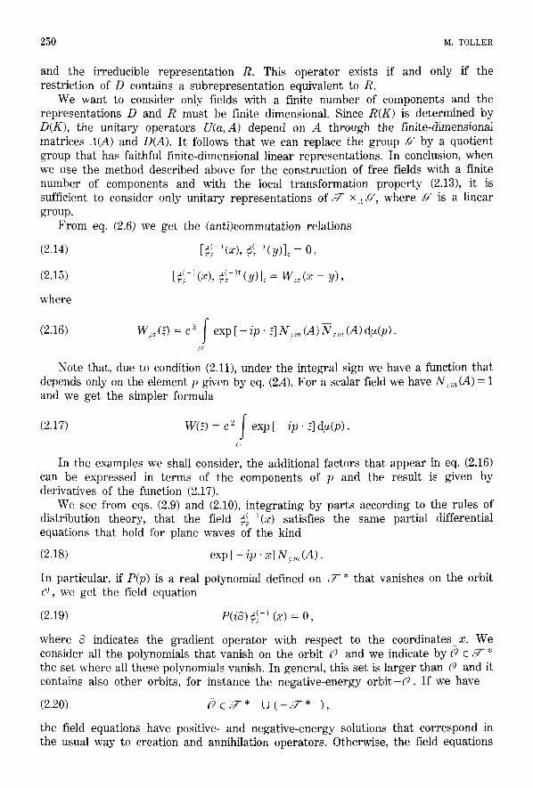
From eq. (2.6) we get the (anti)commutation relations

(2.14) [~(-) (x), "~(-) ..: ~.~ (y)]~ = 0,

(2.15) ~(-) r [~,~ (x), (y)]~ = W ~ ( x - y ) ,

where

f m (2.16) W::(~) = c 2 e x p [ - i p . ?]N~,~(A)N~,~(A)d~(p) .

()

Note that, due to condition (2.11), under the integral sign we have a function that depends only on the element p given by eq. (2.4). For a scalar field we have N, ,~(A) = 1 and we get the simpler folT~ula

(2.17) W(~) = c 2 ~ exp [ - i p . ~] d~(p). . ]

(1

In the examples we shall consider, the additional factors that appear in eq. (2.16) can be expressed in terms of the components of p and the result is given by derivatives of the function (2.17).

We see from eqs. (2.9) and (2.10), integrating by parts according to the rules of distribution theory, that the field r )(x) satisfies the same partial differential equations that hold for plane waves of the kind

(2.18) exp [ - ip �9 x] N~ m (A) .

In particular, if P(p) is a real polynomial defined on J - * that vanishes on the orbit to, we get the field equation

(2.19) P(iS) r (x) = 0, z

where 0 indicates the gradient operator with respect to the coordinates x. We consider all the polynomials that vanish on the orbit (9 and we indicate by (? c ,~ * the set where all these polynomials vanish. In general, this set is larger than (9 and it contains also other orbits, for instance the negative-energy orbit-t0. If we have

(2.20) (~ c J -*+ U ( - J - * + ) ,

the field equations have positive- and negative-energy solutions that correspond in the usual way to creation and annihilation operators. Otherwise, the field equations

FREE QUANTUM FIELDS IN TEN DIMENSIONS WITH Sp(4, R ) SYMMETRY 251

have also -tachyonic, solutions with a doubtful physical interpretation. Then, if we want to introduce an interaction, it may be difficult to avoid the unwanted production of tachyons.

We indicate by ,(/~ the connected complexification of ,(/ and we extend the representation A* to this complex group (it acts on the complexification of the momentum space,~7 "* ). It is clear that if p e (9 and A e ,~'~, the element A* ( A ) p , if it is real, belongs to (~. We shall use this remark to show that in some cases the condition (2.20) is not satisfied.

The local (anti)commutativity properties of the fields have to be discussed separately in the various theories. We expect that a local field is given by

(2.21) r (x) = r + r

where the positive-frequency field r contains creation operators of antiparticles. The two terms in the right-hand side must satisfy the same field equations and have the same transformation property. The vacuum expectation value (Wightman function) of two fields is given by expression (2.15),

(2.22) (/2, r162 = W ~ ( x - y ) .

Since we are dealing with free fields, the vacuum expectation values of the products of more fields can be obtained by means of Wick's theorem. If the field equations and the representation D are real, we can assume that particles and antiparticles coincide and put

(2.23) r +) (x) = r )* (x).

In this case the field (2.21) is Hermitian.

3. - A p p l i c a t i o n to , ( / = Sp(4, R).

The symplectic group ,6~ = Sp(4 , R ) c S L ( 4 , R) is composed of the 4 x 4 real matrices A that satisfy the condition

(3.1) A C A T = C ,

where C is a non-singular real antisymmetric matrix. The elements L of the corresponding Lie algebra ~p(4, R) are real 4 x 4 matrices characterized by the condition

(3.2) L C + C L T = L C - (LC) T = O.

In other words, the matrix L belongs to the symplectic Lie algebra if L C is symmetric and therefore $ = C - 1 L is symmetric too.

In the theories we want to study, the translation group ~ can be identified with the Lie algebra ~p(4, R) and we indicate its elements by means of the real symmetric matrices $. Also the points of the space d" are labelled by symmetric matrices x, y,... and we write, for instance, x - y = ~ e J - . In a similar way, the vectors of the momentum space ~ * can be represented by real symmetric matrices p and we put

(3.3) p- ~ = Tr (p~).

252 M. TOLLER

Since a d ( A ) L = A L A -1 w e have

(3.4) A ( A ) ~ = ( A 1)T ~A-1 , A * ( A ) p = A p A T

The closed invariant cones , ~ + and , 7 +* are composed of the real symmetr ic matrices ~ or p that are positive-semidefinite. This is the only possible choice up to a change of sign [16].

The representa t ions .i and A* are equivalent. The problem of classifying their orbits by giving suitable representa t ive elements is the same as the problem of finding the canonical form, under linear canonical t ransformations, of the quadratic Hamiltonians in classical mechanics. This has been t rea ted in ref.[31, 32] and we summarize the results in appendix B. A more general approach concerning all the real classical Lie algebras is given in ref.[16, 33]. For the present purpose, we have to consider only the orbits with non-negative energy, namely the ones contained in , 7 * +

We indicate by p the generic e lement of the orbit ('~ and by p a part icular representat ive element tha t can be used in order to identify the orbit. Note that the rank r of the matr ix p is invariant under t ransformat ions (3.4) and it is constant over the orbit. Since ~5 is a positive-semidefinite matrix, we can represen t it by means of a formula of the kind

(3.5) )b = .~ ~ ('~) fi '~ v = ~i~ T, .,.~= 1

where u is a 4 x r real matr ix with rank r and the 4 x 1 matr ices/~ (:J) are the columns of it. We consider the constants

(3.6) t:" = - t "," = ~ (')TC - 1 ~ ('.)

that form the r x r ant isymmetr ic matrix

(3.7) t : ~ T C 1 ?~.

The generic e lement of the orbit C~ has the form

(3.8) p = A~bA T = U u T ,

where

(3.9) u = A/~, A e ,0".

We indicate by ('~ ' the set composed of the matr ices u of this form. They satisfy the constraints

(3.10) u T C - l u = t

or, more explicitly,

(3.11) ~ (:~)T C - 1 ?~ (,~) _ t :~' .

Note that all the 4 x r matr ices v with the p roper ty

(3.12) p = v v T


have the form

(3.13) v = u k ,

where k is a real orthogonal r • r matrix. If we require that v satisfies a constraint similar to eq. (3.10), we get the condition

(3.14) k r t k = t ,

that defines a closed subgroup 7[ r O(r), which is clearly compact. An element K of the little group 5~ has the property

(3.15) K ~t(K ~t) T = K[gK T =

and therefore there is an element k �9 q/ with the property

(3.16) K ~ = ~ k .

This formula defines an homomorphism o~-- , 7[. The kernel of this homomorphism is the group ~ ' r defmed by

(3.17) 5 ~ ' = {g �9 G: g ~ = ~}.

The i.u.r.'s of 7! are all finite-dimensional and they provide a class of finite- dimensional i.u.r.'s of ~ We shall see that these are just the i.u.r.'s that permit the construction of free fields by means of the procedure of sect. 2. They have the property

(3.18) Rmn (K) = #ran for K �9 .(X ~ '

and it follows from the covariance conditions (2.2) and (2.11) that the functions f~ (A) and N~m(A) depend on A only through the matrix u =A~, namely they can be considered as functions defined on the set 6) ' = , ~ / ~ ' . Then, eqs. (2.2), (2.11) and (2.12) can be written in the simpler form

(3.19) fm (uk - 1 ) = R~n (k)f~ (u) , u �9 ~) ' , k �9 7 / ,

(3.20) N p ~ (uk) = N ~ , (u) R ~ (k),

(3.21) Npm (Au) = D~ (A) N~m (u), A �9 ,~.

We use the simplified notation R ( k ) = R(K), where K is the element of 5V" corresponding to the element k of 7[.

We indicate by CAB the elements of the matrix C and by C AB the elements of the matrix C-1. When necessary, we adopt the following explicit representation:

(3.22) C = 0 0 0 - 0 1

In sect. 4-9 we consider all the positive-energy orbits listed in appendix B, giving for each of them the matrices ~ (') that determine the representative element ~. In each case, we describe the little group ~ the compact group 7/ and their finite-dimensional i.u.r.'s. Then we discuss the construction of the correspond-

18 - Il Nuovo Cimento B

254 M. TOLLER

ing f ree q u a n t u m fields, giving the i r field equat ions and the i r commuta t i on relat ions.

A f i rs t classification of the orbi ts is p rovided by the i r r a n k r. T h e r e is only one orbi t with r a n k r = 0 and we indicate it by 0) 0. I t contains only the origin p = jb = 0. The little g roup is ,%" =,6 ~ and it has only one f ini te-dimensional i.u.r., n ame ly the trivial one R = 1. I t descr ibes the vacuum.

4 . - F i e l d s f r o m t h e orb i t (~)1"

T h e r e is only one pos i t ive -energy orbi t wi th r a n k r = 1. We indicate it by (91 and we put

(4.1) /t = .

The e lements of ('J1 sa t is fy the polynomial equat ion

(4.2) PA~PcD -- PADPcB = 0

t ha t holds for all the ma t r i ces of r a n k one or zero. As a consequence, we have

(4.3) () ~ = (') ~ U ( - ('~ 1 ) U (') o

and condition (2.20) is satisfied. The e lements of the little g roup ,%" have the fo rm

o (4.4) K = r O a g 1 , r , = • a d - b c = l

0 c - f 0

and the co r r e spond ing e lements of the g roup ~/ /c O(1) a re k = r,. We see tha t ,%" has d imension 6 and the orbi t has d imension 4.

The f ini te-dimensional i.u.r. 's of ,%~' a re one-dimensional and are r e p r e s e n t a t i o n s of ~//. T h e y are given by

(4.5) R/~) (k) = r, ~ , = = 0, 1.

We can sat is fy the condit ions (3.20) and (3.21) by means of the definit ions

(4.6) N(u) = 1, D ( A ) = 1, z = O,

(4.7) N~ (u) = UA , D ( A ) = A , z = 1.

By subs t i tu t ing these express ions into the equat ions of sec t . 2, we ge t the field equat ions and the (an t i )commuta t ion re la t ions of the q u a n t u m fields. We define the componen t s of the g rad i en t o p e r a t o r in the following way:

1 , , c ,D ,D ,C (4.8) ~ABX cD = ~ ~ A ' B + ~AOR).


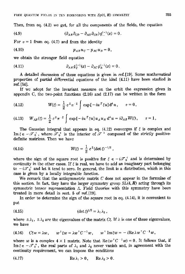
Then, from eq. (4.2) we get, for all the components of the fields, the equation

(4 .9) (~AB ~CD -- ~AD ~CB ) r ) (X) : O.

For ~ = 1 from eq. (4.7) and from the identity

(4.10) PABUC -- PACUB = 0 ,

we obtain the stronger field equation

(4.11) aA8 r -) (x) - oAc r = o.

A detailed discussion of these equations is given in ref. [19]. Some mathematical properties of partial differential equations of the kind (4.11) have been studied in ref. [34].

If we adopt for the invariant measure on the orbit the expression given in appendix C, the two-point functions (2.16) and (2.17) can be written in the form

1 c2r_2 ~ exp[_iuT~u]diu ~ = O, (4.12) W(D = ~

(4.13) WAB(D = ~1 C~rC-2 f exp[_iuT$U]UAUB dau = iaABW(D, ~ = 1,

The Gaussian integral that appears in eq. (4.12) converges if ~ is complex and Im~e - g o + , where g-0 + is the interior of 5 r § composed of the strictly positive- definite matrices. Then we have

1 c 2 (det D- 1/2 (4.14) W(D = ~ ,

where the sign of the square root is positive for $ e - i J - o + and is determined by continuity in the other cases. If ~ is real, we have to add an imaginary part belonging to - i J ' 0 + and let it tend to zero. In general, the limit is a distribution, which in this case is given by a locally integrable function.

We remark that the antisymmetric matrix C does not appear in the formulae of this section. In fact, they have the larger symmetry group SL(4,R) acting through its symmetric tensor representation A. Field theories with this symmetry have been treated in more detail in sect. 5 of ref. [19].

In order to determine the sign of the square root in eq. (4.14), it is convenient to put

(4.15) (det 01/2 = )~I ~2 ,

where _+ 21, -+ ~(~ are the eigenvalues of the matrix C~. If ~ is one of these eigenvahes, we have

(4.16) C$w = 2w, w*~w = 2w*C-lw, w* Im~w = - iRe2w*C- lw ,

where w is a complex 4 • 1 matrix. Note that Re (w* C - l w ) = 0. It follows that, if Im ~ ~ -t~7"o + , the real parts of 2t and 22 never vanish and, in agreement with the continuity requirement, we can impose the conditions

(4.17) Re ~1 > 0, Re ~2 > 0.

256 M. TOLLER

Then we can write

(4.18) 1 W(~) = c 2 (~1),2) -1

The same formula holds when ~ is real, but one has to give a rule tha t determines the signs of ),1 and ),2 when one or both of them are pure imaginary. The rule is that when we add to ~ a small imaginary par t belonging to - i J o + , the pure imaginary eigenvalues must acquire a positive real part .

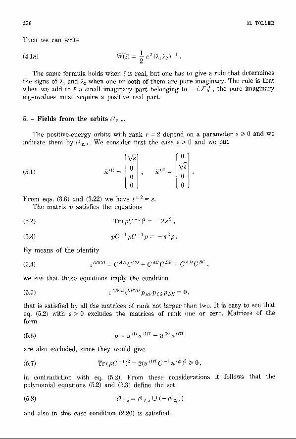
5 . - Fie lds f r o m the orbits (4 2,~.

The posit ive-energy orbits with rank r = 2 depend on a pa rame te r s t> 0 and we indicate them by (~ 2..~- We consider first the case s > 0 and we put

F rom eqs. (3.6) and (3.22) we have t 1,2 The matr ix p satisfies the equations

(5.2)

(5.3)

By means of the identity

(2) =

= S .

T r ( p C 1)2= _ 2 s 2 '

p C - l p C l p = _ s 2 p .

(5.4) ABCD = C A B C C B z[_ c A C c DB + c A D C BC ,

we see that these equations imply the condition

(5.5) ~A~CD~EFGH pBFPCGPDH = O,

that is satisfied by all the matr ices of rank not la rger than two. I t is easy to see tha t eq. (5.2) with s > 0 excludes the matr ices of rank one or zero. Matrices of the form

(5.6) p = u (1) u (1)v - u (2) u (2)v

are also excluded, since they would give

(5.7) T r ( p C -1)2 = 2 ( u ( 1 ) T c lu(2))2 /> 0,

in contradiction with eq. (5.2). F rom these considerations it follows that the polynomial equations (5.2) and (5.3) define the set

(5.8) C~ 2,.~ = (9 ~,,~ U ( - (~z,~)

and also in this case condition (2.20) is satisfied.

FREE QUANTUM FIELDS IN TEN DIMENSIONS WITH Sp(4, R) SYMMETRY

The elements of the little group ~ have the form

(5.9) K =

cosa sina 0 0] - s i n a cosa 0

0 0 a ' 0 0 c

and the corresponding element of ~ = S0(2) is

ad - bc = 1

(5.10) k = [ cosa s ina i . - s i n a cosaj

We see that ~ has dimension 4 and the orbit has dimension 6. The finite-dimensional i.u.r.'s of .(Xf are given by the i.u.r.'s of 7/ and are

R M (k) = exp [2iMa], M = 0, + -1 + - 2 ' _ 1 , . . . . (5.11)

If we put

(5.12) w = u (1) + i u (2),

we can satisfy conditions (3.20) and (3.21) by means of the definitions

(5.13) N ( u ) = 1 , M = O,

(5.14) NAB... (U) = WA W B . . . , (2 I M] terms), M > 0,

(5.15) NAB... (U) = WA W B . . . , (21M I terms), M < 0.

257

Note that the representation D that describes the transformation properties of these quantities and of the fields is the one that acts on the symmetric tensors of order 12MI. Therefore, the indices p,a .... that appear in sect. 2 are replaced by sets of 12M I symmetric S p ( 4 , R ) indices.

It follows from eqs. (5.2) and (5.3) that all the components of the fields defined in this section satisfy the field equations

(5 .16) C TM cBC OAB ~CD r (X) = 2s 2 r (x),

(5 .17 ) C BC C DE OAB OCD ~EF r ) (X) = 8 2 ~AF r ) (X) .

For M ~ 0 from eqs. (5.14) and (5.15) and from the identities

(5.18) p C - l w = i s w , p C - 1 ~ = _ i s ~ ,

we get also the equation

(5.19) cBCOABr ) = +sr M = + IMI . . . - - A . . . - - "

In the scalar case, from the results of appendix C, we get the following expression for the two-point function (2.17):

(5.20) W(D = ~1 c 2 ( ~ _ ~2 )- 1 (~21 exp [ - 2 s~2 ] - ~11 exp [ - 2 S~l ])

where 21, ~2 are the eigenvalues of the matrix C~, which have a positive real part or,

258 M. TOLLER

if they are pure imaginary, acquire a positive real pa r t when we add to ~ a small imaginary par t belonging to - i , ~ o + , as is explained in the preceding section.

By means of the equality

( 5 . 2 1 ) - - T -1 - l p , w w = p - is pC

we get the formula

(5.22) WAB(~) = i(~AB + 8 - 1 c C D ~ A c ~ B D ) W ( ~ ) , M = + 1 - - - - 2

1 Similar formulae can be obtained for I MI > 2"

6. - Fields f r o m the o rb i t (~2,0-

We have to consider one more orbit with rank r = 2, that we indicate by C~ 2, o- We can choose

(6.1) /~ (1) = /~ (2) = Ill and we have t 1.2 = 0. The matr ix p satisfies the polynomial equation

(6.2) pC - 1 p = 0,

that implies eqs. (5.2) and (5.3) with s = 0 and, therefore, also eq. (5.5). Note, however, that eq. (6.2) has solutions of the kind (5.6). The orbit ( ~ , o can be considered as a limiting case of the class of orbits (~ 2, s, but the limit s ~ 0 is r a the r delicate.

We consider the following element of the connected complex group Sp(4, C):

(6.3) A = 0o 0 0 1

0 0

One can easily see that, in the case we are considering, the matr ix AlgA r is real, but it is neither positive nor negative-semidefinite. I t follows f rom the a rgument given in sect. 2 that condition (2.20) is not satisfied. Since the same argument holds for the orbits examined in the following sections, we see tha t only the orbits (~ 1 and (~ 2, ~ with s > 0 have no problems with tachyons.

The elements of the little group ,~/f' have the form

(6.4) K = a 0 1 0 0 d f 1 '

c 0 O 0


where

[c a [ sin o o 2 cos

The element of ?! = 0(2) corresponding to K is jus t k. We see that ,V~ has dimension 4 and the orbit has dimension 6.

The finite-dimensional i.u.r.'s of .r are all representations of ~][. There are two-dimensional representations given by

(6.6) (M) exp[2ina], m, n = -+M, M = 1 1, 3 Rmn (k) = ~m,~,n ~ , ~ , "'"

and for M = 0 we have the one-dimensional representations

(6.7) R (o, :)(k) = V:, a = 0, 1.

By using the notation of eq. (5.12), we can satisfy conditions (3.20) and (3.21) by means of the definitions

(6.8) N ( u ) = 1 , M = O, a = O,

(6.9) N A B ( U ) = Im(WA@B), M = 0, ~ = 1,

f N A B . . . ~ ( U ) = W A W B . . . , (2Mterms) , m = M > 0,

(6.10) ~[NAB...m(U) W A W B . . . , (2Mterms) , m = - M < 0.

All the components of the fields satisfy the equation

(6.11) C Bc aAB aCD r ) (X) ---- O,

that follows from eq. (6.2) and implies eqs. (5.16) and (5.17) with s = 0. The fields that have indices satisfy also the equation

(6.12) ~SC~ ~(-)(X) = 0. ~AB ~ C...

In accord with the results of appendix C, the two-point function for the scalar field is given by

1 22~_12~1()~1 +),2)-i (6.13) W(~) = ~ c �9

The two-point functions of the other fields can be expressed as derivatives of this function by means of the identities

(6.14) Im (WA-WB) I m ( W C W D ) = PACPBD -- PAD P B c ,

(6.15) Re ( W A W B ) = PAB �9

260 M. TOLLER

For instance we have

(6.16) W~BCD(~) = -- (OACS~D -- 8ADOBc) W(~), M = O,

(6.17) WAB(~) ---- 2i0nsW(~), M = 1 . 2

~----1,

7. - F ie lds f r o m the orbi ts (~)3, 8-

The posi t ive-energy orbits with rank r = 3 are classified by means of a p a r a m e t e r s > 0 and we indicate them by C)3, .9. We can choose

ion, [i] (7.1) ~ (1) = ~ ('~) = h (3) = [00 [i] and we have

(7.2) t l , 2 = s , t 2 ' 3 = 0 , t 3 ' 1 = 0 .

The matr ix p satisfies the equations

(7.3) T r ( p C - 1 ) 2 = _ 2s 2 ,

(7.4) T r ( p C - ' ) 4 = 2s 4 .

The elements of the little group ,~K' have the form

(7.5)

cos~ sin~ 0 1 K = - s i n ~ cos~ 0 00

0 0 r, r,a ' r ' = - + l

0 0 0 r , )

and the corresponding element of the group ' 7 / c 0(3) is

(7.6) k = [ cos sins 00] - sin ~ cos ~ .

0 0 r,

We see that .%r has dimension 2 and the orbit has dimension 8. ,%~' is the product SO(2) • • and its finite-dimensional i.u.r.'s are

unidimensional. Some of them contain a factor exp [iha] with h ~ 0, which is not a polynomial function of K. They are not contained in the finite-dimensional representations of Sp(4, R) restricted to the subgroup ,~P and they cannot be used to build local fields by means of the methods of sect. 2. The interest ing representa t ions are the ones that do not depend on a and correspond to i.u.r.'s of '7/. They are given by

(7.7) R (Mz) (k) : , z exp [2iMp], M = 0, + 1 _ ~ , _+1 . . . . , r


I f we use again the notation of eq. (5.12), conditions (3.20) and (3.21) can be satisfied by the expressions

(7.8) N(u) = 1,

(7.9) NAB... (U) = WAWB.. . ,

(7.10) NAB.. (U) = WA WB ... ,

M - - O , z = O ,

(23I te rms) , M > O, ~ = O,

(2Mterms) , M < O, . -- O.

A fur ther factor u~ 3) has to be added to the expressions given above when ~ = 1. F rom eqs. (7.3) and (7.4) we obtain, as in the preceding sections, field equations

that do not involve the indices of the fields. The identities (5.18) hold also in this case and, moreover, we have

(7.11) pC - 1 u (3) __ 0.

F rom these identities we get f i rs t-order partial differential equations similar to eq. (5.19).

The two-point function for the scalar field computed in appendix C is

1 (7.12) W(D ----- -~ C 2 ~ , 1 1 ) ~ 2 1 (~. 2 - - ) 2 ) - 1 sinh (s(21 - )~2)) e x p [ - 8() ,1 + )~2)] �9

The two-point functions for the other fields can be expressed as derivatives of this function by means of the identities

(7.13) W W T = - - is -lpC - lp _ s -2pC -1pC - lp ,

(7.14) u(3)u (a)T = p + s -2pC -1pC - l p .

8. - F i e l d s f r o m t h e o r b i t s 6)4, s, t"

The positive-energy orbits with rank r = 4 are labelled by two parameters s and t, with s/> t > 0 and we indicate them by (9 4, s, t. We consider first the case s > t and we put

[o0] , ~ (3) _-- , ~ (4) _ �9

We have

(8.2) t l 'e = s, t s'a = t , t '~ = 0, /~ = 1, 2, v = 3, 4.

The matr ix p satisfies the equations

(8.3) T r ( p C - 1 ) 2 = _ 2(s z + t2 ) ,

(8.4) Tr(pC-1)4 _ 2(s a + t 4 ) .

The elements of the little group c~, tha t coincides with the group ~]! r O(4), have

262 M. TOLLER

the fo rm

cos sin O 0 ~ ] (8.5) K = k = - s i n ~ cos~ 0

0 0 cos~2 s in9

O 0 - sinfi cos,2J

We see t ha t .%~' has d imension 2 and the orbi t has d imension 8. ~// = .%~' is the p roduc t SO(2) • SO(2) and its i.u.r. 's a re unidimensional and given

by

R (M'M") (k) = exp [ 2 i M ' :~ + 2 i M " 2 ] M ' M " = 0, + _1 _ 1, . . . . ' ' ' - 2 '

(8.6)

I f we pu t

(8.7) w (1) u (2) + i n (2) w (2) = u (3) + i u (4)

conditions (3.20) and (3.21) can be sat isf ied by express ions of the kind

(8.8) NA ~ ( u ) = o (1) o,(2) , , , . ...... ~ a . . . . . B . . . . (21M 1 + 2 1 M " I t e r m s ) , M M " > O

F o r nega t ive values of M ' or M " , the vec to r s w (1) or w (2) have to be rep laced by the i r complex conjugated , as in eq. (5.15).

F r o m eqs. (8.3) and (8A), we ge t field equat ions t ha t do not involve the indices of the fields. Other field equat ions of the f i rs t o rde r involving the field indices follow f rom the identi t ies

( 8 . 9 ) lp C - 1 U) (1) : iSW (1) , pC - 1 ~ (1) = - - i S W (1) ,

[ p C - 1 w (2) i t w (2) , p C - 1 ~ (2) = _ i t ~ (2) .

The two-poin t function for the sca lar field compu ted in appendix C is

1 c 2 ) ~ 1 ) , ~ 1 ( ) , ~ _ ),~)_~ sinh ((s - t)(~,~ - )~2)) exp [ - ( s + t ) (~ + )~2)]. (8.1o) w(~)=

The two-point funct ions of the o the r fields can be compu ted in t e r m s of der iva t ives of this function by m e a n s of the identi t ies

(8.11) w ( 1 ) ~ (1)T = ( t ~ - s 2) l ( t e + ( p C - 1 ) 2 ) ( 1 - i s lpC-1)p,

(8.12) w(2)~ (2 ) r= ( s 2 - t 2) l ( s ~ + ( p C - 1 ) 2 ) ( 1 - i t 1 p C 1 ) p .

9 . - F i e l d s f r o m t h e o r b i t s (~ 4, s, ~ .

We have to consider ano the r orbi t wi th r a n k r = 4, tha t we indicate by (~) 4, ,~, ~ (s > O). Equa t ions (8.1)-(8.4) a re still valid if we put t = s, bu t the ma t r ix p satisfies the condition

(9.1) ( p C - 1 ) 2 = _ s 2 ,

t h a t is s t r o n g e r than eqs. (8.3) and (8.4).

F R E E QUANTUM F I E L D S IN T E N D I M E N S I O N S W I T H Sp(4, R) SYMMETRY 2 6 3

The elements of the little group ~ , that coincides with the group ~! r 0(4), have the form abc!] (9.2) K = k = - b a - d a + i b c + i d = i f e U ( 2 ) .

e f g ' e + i f g + i h

- f e - h

We see that , ~ has dimension 4 and the orbit has dimension 6. The i.u.r.'s of U(2) are all fmite dimensional and act on the symmetric spinors

with 2S indices in the following way:

(9.3) [R (MS)(k)f]m ' " = (det K) M ifmm .... i f ~ 'f~' ...n',

1 S = O , ~ , 1 . . . , M = O , +1, . . . .

For i f �9 SU(2), these are the usual representations with spin S. If we adopt the notation of eq. (8.7), we can satisfy conditions (3.20) and (3.21) by means of the expressions

(9.4) NA...8 ~.... (U) . . . . (m) ~"(') (2S terms), M = 0, ~ ( A . . . . B) '

where the parenthesis indicates the symmetrization with respect to the indices (A... B). If M > 0, we have to add M factors of the kind ~,, (1)o,, (2) . . . . (2) ~,,(1) and if W A W B W A ~ B M < 0 we have to add ]M] complex conjugated factors of the same kind.

From eq. (9.1) we get a field equation that does not involve the field indices. From the identities (8.9), that hold also in this case with t = s, we get

(9.5) C BC OAB r ). (x) = +- sr (x),

where the sign depends on the nature of the index A. The two-point function for the scalar field computed in appendix C is

1 (9.6) W(O -~- "~- C 2 ~ 1 1 2 2 1 ( 2 1 4" 2 2 ) - 1 exp [-2s(21 + 22)].

The two-point functions of the other fields can be expressed as derivatives of this function by means of the identities

(9.7) w (1) @ (1)T + W (2) @ (2)r = p _ is - 1pC - 1 p ,

(9.8) (o,, (1) a,, (2) _ a,, (2) a,, (1) ~{~-~ (1) ~ (2) _ ~ (2) ~ (1) ~ _ X ~ A ~ B ~ C ~ D / ~ A ~ B ] x ~ C ~ D

= (p - is -1pC- lP)AC( p -- i s - l p C - l p ) B D - - ( p - - i s - l p C - l P ) A D ( P -- i s - 1 p C - l p ) B c .

10. - Causa l i n d e p e n d e n c e and causa l in f luence .

Now we want to analyse the theories introduced in sect. 4-9 from the point of view of local (anti)commutativity. We consider first the scalar fields corresponding to the various orbits. The (anti)commutator functions W(D (see eq. (2.17)) have been

264 M. TOLLER

computed in appendix C in terms of the quantities )~ and he, where -+ ~ and _+ ~2 are the eigenvalues of the matrix C~. As we have explained in sect. 4, we choose the signs of the quantities )~1 and ),2 by requiring that their real parts are positive. I f one of these quantities lies on the imaginary axis, we require that it acquires a positive real par t when we add to ~ a small matrix belonging to - i , ~ o + .

We consider the open set ,Pc = - ~ c c ~ defined by requiring that the matrix C~ has no eigenvalues on the imaginary axis. When ~ ~ -~, the eingenvalues of C~ do not change and, if ~ e , ~ c , the quantities ),~ and ),2 remain the same. Therefore, we have

(10.1) W(~) = W( - ~) for ~ e , ~ c -

One can easily see that if, for instance, ),~ is imaginary, according to our rules its sign changes when ~---> - ~ and eq. (10.1) does not hold any more, unless )~ = - ),2 or ).~ = 0. Since eq. (10.1) has to be considered in the sense of distribution theory and it is meaningful only if ,-7- c is open, we have to disregard this possibility.

The situation is different for the function (4.18), that depends on the product ),~ ),2. In this case, eq. (10.1) holds also when both ;~ and )~2 lie on the imaginary axis. This s t ronger proper ty is a consequence of the larger symmetry group GL(4,R) of the orbit ('] ~.

We have seen that the (anti)commutator functions W.=(~) of the fields of the general kind can be written in terms of derivatives of the functions W(~) of scalar fields. We remember that the indices ~, ~- stand for sets composed of N Sp(4, R) indices and we see by direct inspection that we have

(10.2) W=(D = (-1)~VW~:(-~) for ~e J - c �9

Since in all the theories we have considered the representat ion D and the field equations are real, we can introduce the Hermitian local fields

(10.3) r = ~( - ) (~ + ~(-)*(x).

As a consequence of eq. (10.2), they satisfy the local (anti)commutativity proper ty

(10.4) [r162 for x - y e J ' c , ~ = ( - - 1 ) N+I

Note that this equation holds only if there is a connection between , sp in , and statistics, namely

(10.5) s D ( - 1) = - 1.

If x - y e , ~ c , we say that the two points x and y are causally independent. Besides the open invariant set J - c , the vector space ~ contains also the two closed invariant cones ~ § and - , ~ § . We want to show that the matrix ~ belongs to J -0 + (the interior of ~ § ) if and only if both ~1 and ~2 lie on the positive imaginary axis. F rom eq. (4.16) we see that if ~ E ,~7-0 + , ~1 and ~ are non-vanishing and imaginary. From the classification of the orbits in J - given in appendix B, we find that this proper ty is t rue for the representat ive elements of the kind (B.6) and for the ones composed of two blocks of the kind (B.2). A straightforward analysis of these cases shows that ~ is positive-definite if and only if ~ and ~2 are on the positive imaginary axis.


I t follows from the result given above that ~ ' c and J -0 + do not overlap. Since ~J-c is open and 5 r § is the closure of 5r0+ we have

(10.6) ~ - c N 5 r § = 0 .

However, it is not t rue that

(10.7) . ~ -cU .~ + U ( - , ~ + ) = J ",

as it happens for the relativistic theories in Minkowski space. This is an important new feature of the theories we are-Considering.

A similar situation, with a different definition of the set J ' c has been discussed in ref.[12, 19] in the framework of SL(4, R)-invariant theories, by introducing an invariant closed set J ' w c ,~" with the propert ies

(10.8)

(10.9)

(10.10)

The relations x - y �9 ~ - +

5 rc n 5rw = 0,

~J'c U .~-w U ( -~q-w) = J ' ,

5 r w + ~ + = ~J-w.

and x - y �9 ~ r W are called, respectively, strong and weak causal influence. Note that, since 5 r W is not a wedge, the relation of weak causal influence is not transitive. The set

(10.11) 5rR = 5rW n ( - ~Srw )

is larger than {0} and the relation x - y �9 ~ R is called reciprocal (weak) causal influence. As discussed in ref.[12, 19], it replaces the space-time coincidence in non-local theories.

We want to show that a similar scheme can be introduced for other field theories, in particular for the Sp(4, R)-invariant theories t rea ted in the present paper. We s tar t form the general definition

(10.12) J ' w = C(,~-c - ~" § ),

where C means the complement of a set. We assume that ~ § is an invariant closed cone, t h a t S r c = - 5 r C is invariant and open and that eq. (10.6) is true. Then it is easy to show that 57- W is invariant and closed and has the propert ies (10.8) and (10.10). The proper ty (10.9) is equivalent to the condition

(10.13) (St c - ~7" + ) n (~7-c + 5 r + ) = pT- c .

I f we consider 5 r as an ordered vector space with positive cone 5 r § this formula means that the set 5 r c is order-convex[35].

The property (10.13) justifies the definition of the time-ordered product given by

(10.14) Ir r if x - y �9 5 rc + ~ - + ,

T(r r = [r162 if x - y �9 ~7"c - ~ +

266 M. TOLLER

Note that this distribution is defined on the complement of the set J R defined by eq. (10.11), which plays an important role in a perturbat ive t rea tment of interactions.

In order to show that this general scheme applies to our Sp(4, R)-covariant theories, we have to prove eq. (10.13). I t is convenient to introduce the invariant function

(10.15) F(~) = Im (21 + 22)

and to show that it is continuous and non-decreasing on the ordered vector space J , namely that it has the proper ty

(10.16) F(~ + ~+ ) t> F(~), ~ e ,~7, ~+ �9 ,~7 +

If 21 has non-vanishing real and imaginary parts, we have 22 = ~1. I t follows that only pure imaginary eigenvalues contribute to F(~). I t is clear that F(~) is continuous at the points where there are not multiple imaginary non-vanishing eigenvalues. The eases where the eigenvalues are imaginary and 21 = -+ 2e have to be examined separately. By using the characterization of J -0 + given above, it is easy to show that F(~) is continuous also at these points.

We put

(10.17) ~ ' = ~ + 3 ~ + , ~ � 9 ~+�9 + , 31>0

and we indicate by 2(3) a (possibly multiple) eigenvalue of C~'. We have to show that its contribution to F(~') is a non-decreasing function of 3. I t is sufficient to consider arbitrari ly small values of 3 and we can assume that 2(:) is imaginary, otherwise, as we have seen, its contribution vanishes or it is cancelled by the contribution of another eigenvalue. The eigenvalues are solutions of a biquadratic algebraic equation and are given by the formula

1[ ] (10.18) 2(3) = _+ ~ T r ( C y )2 _+ ((Tr (C~')2)2 _ 16det~' )1/2 1/2.

I t follows that for = ~ 0 we have the asymptotic behaviour

(10.19) 2(3) - 2(0)=ic3 ~ , ~ > 0.

If c is not real, 2(3) is not imaginary and it does not contribute to F. If c is real and we add to r a small negative imaginary part, 2(=) acquires a real par t of the same sign as c. According to our rules, 2(3) is one of the eigenvalues 21 or 22 only if c is positive and eq. (10.16) is proven for ,:+ �9 ,~To + . A continuity argument shows that it is t rue in general.

Note that for ~ �9 J - c we have F(~) = 0. The same equality may hold also if C~ has imaginary eigenvalues, but then, by examining the representat ive elements of the orbits that have this property, we can show that a small perturbat ion of ~ is sufficient to get F(~) e 0. In other words, J - c is the interior of the set where F(D vanishes. Since F is non-decreasing, this set, and therefore its interior too, is order-convex and eq. (10.13) is proven.

There is another characterization of the set 7 C which holds for the theories examined here and for the ones described in ref. [12, 19], but is meaningful for any choice of the group ,6 ~. We say that the orbit 5 ~ is symmetric if 6 ~ = - C. It is easy to


see that ~ ' c is composed of symmetric orbits and that on all the symmetric orbits we have F(D = 0. It follows that ~z- C is the interior of the union of all the symmetric orbits. It would be interesting to know if the set 5rc defined in this way is order- convex also for other choices of ,~.

We see from defmition (10.12) that the points where F(D is positive belong to 5~'w. By examining the representative elements of the orbits contained in ~Jw where F(D = 0, we see that they can be approximated by elements with F positive. It follows that 5rw is just the closure of the set defined by F(O > 0. The set ~J'R defined by eq. (10.11) is composed of the points $ where F(D vanishes, but it can be made both positive and negative by means of small perturbations of ~. A detailed analysis shows that the representative elements of the orbits that have these properties are the following: [ oo (10.20) ~= 0 b 0 b > 0

0 - b ' 0 0 - [ oo

(10.21) ~ = 0 0 a t > 0 , 0 0 ' 0 a

0 o 0 0 0 - 1 ' | 0 0 0 " 0 0 0 0

The orbits described by eq. (1021) form a set composed of the elements of the form

(10.22) ~ = u (1) u(1)z - u (2) u (2)r,

where u (1) and u (2) are (possibly vanishing) 4 x 1 real matrices. This is the set ~z" R one gets from SL(4, R)-invariant theories, that has been described in ref. [12]. The orbits given by eq. (10.20) are described in appendix D, where we show that their appearance does not introduce essential changes in the discussion of ref. [12].

A P P E N D I X A

Projec t ive representa t ions .

In this appendix we show that if the Lie algebra I of the connected Lie group G is semisimple and A is the adjoint representation, the unitary projective representations of the semidirect product _~ = 5r x A,6~ ~ e generated by unitary representations of its universal covering group_~ = 5z" x ~,~. A similar property holds, as is well known[23, 26], for the Poincar6 group in three or more space-time dimensions, but not for the Galilei group and for the Poincar6 group in two space-time dimensions.

268 M. TOLLER

According to the treatment of ref. [23], we have to consider the Lie algebra jo of _(d and show that all the infinitesimal exponents are equivalent to zero. We remember that an infinitesimal exponent is an antisymmetric bilinear form ,2(R, R ' ) , R, R ' � 9 .(', that satisfies the condition

(A.1) 2([R, R ' ] , R" ) + ~([R' , R "], R) +,3([R", R], R ' ) = 0.

In the language of cohomology theory[36, 37], ,2 is a cocycle. Two cocycles are equivalent (cohomologous) if their difference has the form

(A.2) ,2(R, R ') - ,s' (R, R ') = ~([R, R ' ] ) ,

namely it is a coboundary. The equivalence classes of cocycles form the cohomology group H 2 (-7') and we have to show that it contains only the zero element.

In the problem we are considering,-7' is the semidirect sum Y]-@~ [ of considered as an Abelian Lie algebra and the Lie algebra { of the Lie group .(/, namely we have

(A.3) [ L + a , L ' + a ' ] = [ L , L ' ] + A ( L ) a ' - A ( L ' ) a , L , L ' � 9 a , a ' � 9

where L--~A(L) is the representation of [ acting on ,-7, corresponding to the representation g ~ A(g) of the group ,0".

If we assume that [ is semisimple, we can use a general theorem, given in ref.[37], p. 439, which gives the cohomology groups H " ( , ~ @ ~ [ ) in terms of the cohomology groups H ' ( , 7 ) and H ' ( [ ) . Since { is semisimple, we have HI(I)= = H2([) = {O} and we get the simple formula

(A.4) H 2 ( , ~ | = H2(,~)I ,

where H 2 (,-7)t is the subspace of H 2 (,~) composed of the elements invariant with respect to natural action of the group ,0 ~. Since the Lie algebra J is Abelian, the right-hand side of eq. (A.4) is just the space of the bilinear antisymmetric forms on ,~ with the invariance property

(A.5) ~(A(L) a , a ' ) + ~ ( a , A ( L ) a ' ) = 0 , L e l , a , a ' e ,~7" .

If A is the adjoint representation, we can identify ,~ and { and eq. (A.5) takes the form

(A.6) fl([L, L ' 1, L" ) + fl(L ', [L, L "]) = 0.

By using several times this formula together with the antisymmetry of fi and of the Lie product, we get ~(L,[L'L"])= 0. Since the elements of the form [L ' , L"] generate the vector space 1, we have H2(J ~ = {0} as we wanted to show.

APPENDIX B

Orbits of the adjoint representation of Sp(4, R).

For convenience of the reader, we give the list of the representative elements of the orbits of the adjoint representation of Sp(4, R), according to the classification given in ref. [31, 32]. We use the conventions given in sect. 3 and a choice of the representative elements slightly different from the one adopted in the references


quoted above. The same results hold for the coadjoint representation. We give also for each representative element ~ the eigenvalues 21 and 22 of C~, with the choice of the sign explained in sect. 4 and 10.

Some representative elements are composed of two diagonal blocks chosen among the following kinds of 2 • 2 matrices; The eigenvalues 21 and he are determined separately by the two blocks:

(B.1) I~ ~}' +-[~ ~1' 21=0,

(B.2) -+I~ ~]' b > 0 , ~ : = + i b ,

(B.3) [0a 0]' a > 0 , 21=a.

Only the matrices (B.1) and (B.2) are positive- or negative-semidefinite. The other representative elements have one of the forms [ 00

(B.4) + 0 0 21 -- 2 2 ---- 0 , 0 0 ' 1 0

(B.5) a 0 0 0 0 , a > 0 , 2 1 = 2 2 = a ,

0 a [ oo (B.6) + 0 - b b > 0 , 2 l = i b 2 z = - i b

- - b 1 ' ' '

0 0

a o:] (B.7) a 0 - b

- b 0 , a , b > 0 , 21 = a + ib,

0 a

he = a - ib.

The matrices (B.4)-(B.7) are neither positive- nor negative-semidefmite.

A P P E N D I X C

I n v a r i a n t m e a s u r e s a n d i n t e g r a l s o n t h e o r b i t s .

It is known[22] that an orbit O of the coadjoint representation A* has a symplectic structure defined by a closed non-degenerate 2 form ~ given by the formula

(C.1) (o(X(L), X(M)) = p . [L, M], L, M �9 l, p �9 ~*.

270 M. TOLLER

We have indicated by X(L) the vector field on 5) that generates the infinitesimal transformations corresponding to the element L of the Lie algebra [.

If the orbit 5) has dimension 2m, the Liouville invariant measure is given by the differential form

(C.2) ~2 - 1 - - (o A ... A (,~, (m factors). m! (2=)"

The normalization factor that appears in this formula is the one that simplifies some fur ther developments of the theory [20, 22].

In sect. 3 we have defined, for each positive-energy orbit 5) with rank r, a set (9 ' composed of 4 • matrices that satisfy the constraint (3.10). The group ,(/ acts transitively on both 5) and 5) ' and eq. (3.8) defines a mapping 5 ) ' - ~ 5) equivariant with respect to the action of ,(/. The inverse image of a point p e 5) is an orbit of the action of a compact group ~/! on ('~ ' . We indicate by (,)' the pullback on 5) ' of the 2 form co. If we indicate by X ' ( L ) the vector field on 5) ' that generates the infinitesimal transformation corresponding to L, (o' is characterized by the formula

(C.3) o / ( X ' (L), X ' (M)) = ~o(X(L), X(M)) = p . [L, M] = Tr (pC 1 [L, M]) .

From the formula

(C.4) du (A '~) (X' (L)) = L Bu~ ~) ,

we see that eq. (C.3) is satisfied by

( c . 5 ) = - A " ) .

f,z= 1

This formula permits the calculation of the pullback t2' of ~9 and of the invariant measure on 5). We shall not give here the details of this calculation.

We remark that a funct ionf(p) defined on 5) can be considered as a funct ionf(u) = = f ( u u T) defined on (9 ' that satisfies the condition

(C.6) f(uk) = f (u ) , k e ~ / .

I f j ~ has compact support, f has the same proper ty and we get an invariant measure on 5) by means of the formula

( C . 7 ) f f(p)d,~(p) = c' (~) I f(u) I-[ 1~<,~ <,~ ~< r

(9

~](U ~,~)T C - 1 u (~) - t ,'~'~ ) d4ru.

Since the invariant measure is unique up to a numeric factor, we have only to compute c ' (5) ) by means of eq. (C.5). The result is

(C.8) f l 1 __-2 '(5)1)= ~ , . ,

1 '(5)3,s) = ~ ~-~s,

, 1 ' ( ( 9 1 ~ 4 (5) 2, s ) : ~ 77 4 , C 2,0) = ~- ,

1 1 C'(5) 4, s, t) -~ "~ ~ 6(82 -- t2), C'(5) 4, S, s) ~- ~ ~ -68"

The commutation function (2.17) has been computed in sect. 4 for the orbit (91 and


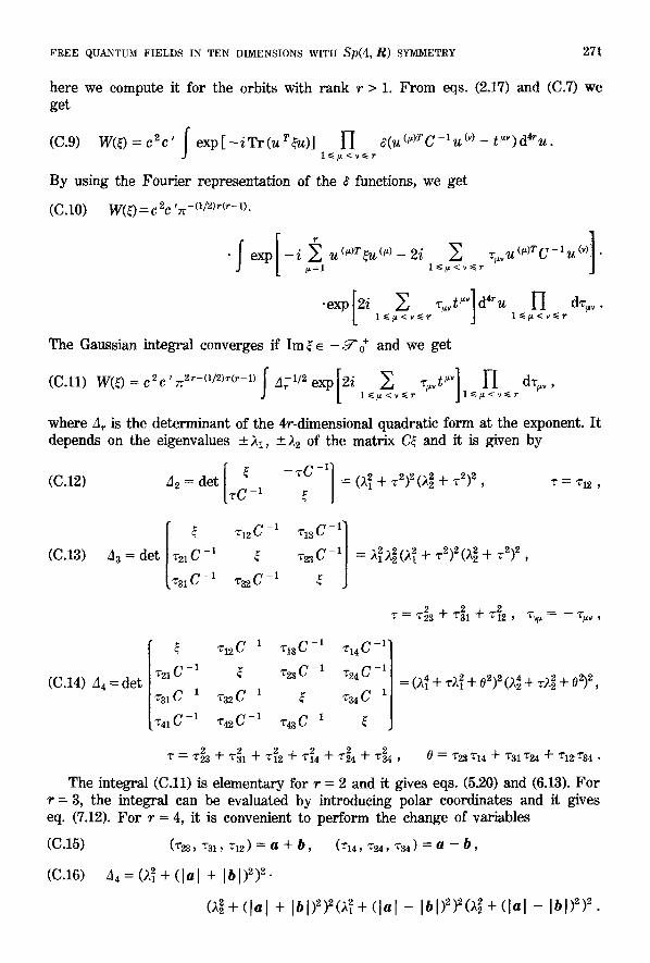
here we compute it for the orbits with rank r > 1. From eqs. (2.17) and (C.7) we get

(C.9) W(s = c2c ' f exp[-iTr(ur~u)] ~ a(u(')rC-lu(~) - t~')d4~u. J

By using the Fourier representation of the ~ functions, we get

W(~) = c 2c 'zr-(1/2)r(r- 1).

Iex0[ (c . to)

u (~) r0z ( ' ) - 2 i ~ r , ,u ( ')Tc-lu(@] " /~=1 1~</~ <v~<r

The Gaussian integral converges if Im~ e - ~ o + and we get

(C.11) W(~)=C2C'rr2r-(I/2)r(r-1)I Arl/2exp[2i 1~<~ < ,<rE ~'~v t~tv]l~<t L<v~<rl'I d'rt~,,

w h e r e A r is the determinant of the 4r-dimensional quadratic form at the exponent. It depends on the eigenvalues -+21, -+22 of the matrix C~ and it is given by

(C.12) A 2 det [ ~ --TC-1] = = 0,12 + .:2)~ (~,~ + ,r2)2, ~" = 'r12, ~ C -1

T13 C - 1"

T23C -1 (C.13) ~3 = det

~ T12 C - 1

"{'21 C - 1

'r31 C - 1 'r32 C - 1

= ~12 ~'22 (~2 .Jr T2)2 ()t2 _}- ,V2)2

C -1 Tt3C -1 T14C -11 T12

-I ~ ~23C -1 T24C-11 (C.14) A 4 : d e t ; : : C _ 1 ~326 -1 $ ~a4 C -11 "

tT41C -1 T42C -1 T43C -1 ~,

= (z~ + ~z~ + 02) 2 (z~' + ~zl + 052,

T ---- T 2 -l- T231 -~- T22 -l- T24 -~- T224 -[- T234 , 0 :- T23 T14 -I- 231 224 -[- T12 ~'34

The integral (C.11) is elementary for r = 2 and it gives eqs. (5,20) and (6.13). For r = 3, the integral can be evaluated by introducing polar coordinates and it gives eq. (7.12). For r = 4, it is convenient to perform the change of variables

(C.15) (~'23, 2"31, 2"12) = a + b , (~',4, T24, 7"34) ---- a - b ,

(C.16) A 4 _ (~2_]_ ( ]a ] + Ib[)2) 2.

0 ~2 + ( l a l + Ib[)2)2(~, 2 + ( l a [ - Ib l )2)20 ,~ -t- ( l a l - Ibl )2) 2 .

272 M. TOLLER

Then the integration can be performed in polar coordinates and we get eqs. (8.10) and (9.6).

APPENDIX D

Prope r t i e s o f the set .~Y-w-

In this appendix we show how the description of the set J -w given in ref. [12] has to be modified when we deal with the field theories considered in the present paper. As in ref. [12] (but with slightly different conventions), we write the matrix ~ E ~ in the form

(D.1) : = 1 bkC_ iyk + 1 brsC_l

where we indicate by ~.% (k = 0, 1, 2, 3) the real Dirac matrices in the Majorana representat ion that satisfy the condition

(D.2) :.~ = - C - ' ~'k C.

We adopt the metric tensor goo = - 1, g,1 = g22 = gs~ = 1. The Lorentz group that acts on the indices i ,k ,r ,s , ... (more exactly, its universal covering SL(2, C)) can be considered as a subgroup of Sp(4, R). We introduce also the three-dimensional vectors

(D.3) b = (b 1, b 2, b '~ ), b ' = (b 2a, b 3', b ,2), b " = (b 10, b 20, b 30).

By means of a suitable Lorentz transformation, these quantities can be put in the form

(D.4) b ' = (0, 0, ~), b" = (0, 0, rj), ~2 + f12 > 0,

(D.5) b ~ = t , b = ( , : cos r ,~sin r r ) , ,z i> 0.

There is also a degenerate case in which eq. (D.4) has to be replaced by

(D.6) b ' = (a, 0, 0), b" = (0, ~, 0), a ~> 0.

It has been shown in ref. [12] that in the generic ease (D.4), (D.5), the set defined by eqs. (10.21) or (10.22) is characterized by the condition

(D.7) t = 0, ~- -- 0, ~ = ~ + f12,

while in the degenerate ease (D.4), (D.6), the condition is

(D .8 ) ,o = 0 , t = I YI <

We have to take into account also the points belonging to the orbits with representat ive elements of the kind (10.20). They satisfy the condition

(D.9) (Cx)2 = - s 2 ,


that, by means of eq. (D.1), can be written in the form

1 (D.10) b~bk - -~ brSbr~ = - 4s 2 , sikr~b~kb ~ = 0, eikrsbkb rs = O,

or

(D.11) (b~ ~ - Ib12+ I b ' l 2 - Ib"12- -4s 2 , b ' . b " = O , b . b ' = O , b " • 1 7 6 '

This condition is not sufficient to characterize the class of orbits we are considering, since it is satisfied also by the orbits -+ O 4, s, s described in sect. 9. I t is sufficient to add the requirement that $ has two positive and two negative eigenvalues. From the results of ref. [12], we see that in the generic case (D.4), (D.5), this leads to the inequality

(D.12) t 2 < (• _ V~a~ + f12)~ + ],2,

while in the degenerate case (D.5), (D.6), we get

(D.13) ~ - ~/(a - ~,)~ + p2 < t < - a + ~r + y)2 + p2.

A detailed analysis of eqs. (DA)-(D.6) and (D.11)-(D.13) shows that the orbits with representative elements of the kind (10.20) exist only in the generic case (D.4), (D.5) under the conditions

(D.14) t =f l = ], = 0, 0 ~< ~ < ~.

In conclusion, the difference with the case analysed in ref. [12] is that for fl = 0 the circumference defmed by eq. (D.7) is replaced by a circle. Then, most of the conclusioas of ref. [12] concerning the set 57" W remain valid.

R E F E R E N C E S

[1] TH. KALUZA: Sitzungsber. Preuss. Akad. Wiss. Berlin, Math. Phys. K, 1, 966 (1921). [2] O. KLEIN: Z. Phys., 37, 895 (1926). [3] C. A. ORZALESI: Fortschr. Phys., 29, 413 (1981). [4] W. MECKLENBURG: Fortschr. Phys., 32, 207 (1984). [5] M. J. DUFF, B. E. W. NILSSON and C. N. POPE: Phys. Rep. C, 130, 12 (1986). [6] S. KOBAYnSHI and K. NOMIZU: Foundations of Differential Geometry (Wiley, New York,

N.Y., 1969). [7] Y. CHOQUET-BRUHAT: Ggomgtrie diffdrentielle et syst~mes extdrieurs (Dunod, Paris,

1968). [8] M. TOLLER: Nuovo Cimento B, 44, 67 (1978). [9] G. COGNOLA, R. SOLDATI, M. TOLLER, L. VANZO and S. ZERBINI: Nuovo Cimento B, 54, 325

(1979). [10] Y. NE'EMAN and T. REGGE: Riv. Nuovo Cimento, 1, n. 5 (1978). [11] M. TOLLER: Nuovo Cimento B, 64, 471 (1981). [12] M. TOLLER: Int. J. Theor. Phys., 29, 963 (1990). [13l S. WEINBERG: Phys. Lett. B, 138, 47 (1984). [14] I. E. SEGAL: Mathematical Cosmology and Extragalactic Astronomy (Academic Press,

New York, N.Y., 1976). [15] E. B. VINBERG: Funct. Anal. Appl., 14, 1 (1980). [16] S. M. PANEITZ: J. Funct. Anal., 43, 313 (1981).

274 M. TOLLER

[17] E. INONU and E. P. WIGNER: Proc. Natl. Acad. Sci. U.S.A., 39, 510 (1953). [18] F. LUR~AT: Physics, 1, 95 (1964). [19] M. TOLLER: Nuovo Cimento B, 102, 261 (1988). [20] M. TOLLER: University of Trento preprint UTF 271 (1992). [21] HARISH-CHANDRA: Trans. Am. Math. Soc., ll9, 457 (1965). [22] A. KmILLOV: Eldments de la thdorie des reprgsentations (Editions MIR, Moscou, 1974). [23] V. BARGMANN: Ann. Math, 59, 1 (1954). [24] F. WILCZEK: Phys. Rev. Lett., 49, 957 (1982). [25] J. FROHLICH and P. A. MARCHETTI: Lett. Math. Phys., 16, 347 (1988). [26] E. P. WIGNER: An~. Math, 40, 149 (1939). [27] G. MACKEY: Bull. Am. Math. Soc., 69, 628 (1963). [28] M. FLATO and C. FRONSDAL: Lett. Math. Phys., 2, 421 (1978). [29] J. FANG and C. FRONSDAL: Lett. Math. Phys., 2, 391 (1978). [30] C. FRONSDAL: Phys. Rev. D, 20, 848 (1979). [31] J. WILLIAMSON: Am.. J. Math., 58, 141 (1936). [32] V. ARNOLD: Mgthodes mathgmatiques de la mdcanique classique (Editions MIR, Moscou,

1976). [33] N. BURGOYNE and R. CUSHMAN: J. Algebra, 44, 339 (1977). [34] L. GARDING: Ann. Math., 48, 785 (1947). [35] G. JAMESON: Ordered Linear Spaces (Springer-Verlag, Berlin, 1970). [36] C. CHEVALLEY and S. EILENBERG: Trans. Am. Math. Soc., 63, 85 (1948). [37] W. GREUB, S. HALPERIN and R. VANSTONE: Connections, Curvature and Cohomology,

Vol. III (Academic Press, New York, N.Y., 1976).

Documents

Free quantum fields in ten dimensions withSp(4,R) symmetry