Introduction. 

Syllabus   Can we meet Fridays, instead of Thurs? 

General thoughts. 

This class is usually taught by theorists.    I am not a theorist.    But I use QM in my work a lot and am 

very comfortable with it.    Point is I am not quite familiar with all the things that theorists find useful to 

concentrate on.   Example Charlotte told me everyone should use del notation/ϵijk  I agree.   Everyone 

should work out the group multiplication for all the angular momentum states.   I don’t agree so maybe 

we won’t concentrate on that quite as much.   

In fact last year we didn’t make it to Chapter 3: ( this year is different, this year we must.  )  Gives you an 

idea of the pace of the course.    This course will cover approximately Ch‐1‐2 and some decent fraction 

of Ch 3. of Sakurai.  Then there will be several other special topics 

Therefore do not expect to move through  Sakurai quickly.  We will go very slowly through it.   I 

recommend reading the entire 1st Chapter quickly, then for my “reading assignments” go back and 

carefully restudy.  

How fast we can move will be partially dependent on you guys.    I will be quizzing you along the way, 

both formally and informally.   

I’d like to cover somethings related to my research, of Heavy Ion physics, but probably the most relevant 

thing is scattering which we won’t get to in this course.  

Didn’t make it there last year though:  Instead I’d like to teach a little about quantum entanglement and 

perhaps quantum computation.  

 

Still, we will approach lectures a little differently.  We will try having a day (Friday) where we do 

problems in groups.  

 

The Web: 

There is a lot out on the web, including solutions to many problems in Sakurai.  Remember about 

cheating.   Personally I don’t care as long as you understand the solution.  

I recommend Wikipedia for many subjects.  I have been referring to it  for preparation for this class.  You 

can find quite a bit of detail on it.  e.g. Mathematical Definitions.   

 

 

I will put links occasionally, some for reference and some will be required reading.  

At least at one point during the semester (possibly 2), I may want to meet with some or all of you 

individually, sometime after the first few weeks of the quarter.  These will be 15‐30 minute 

“conferences” and we will discuss your plans,your performance in the class, specifically any homework 

problems or midterm problems you may not have done so well on.  

I will call on people specifically to answer questions sometimes.  This will be part of your participation 

grade.  I will go through the list of names in alphabetical order so I will let you know when your turn is 

up, and you should try to be in class those days.   

 

Reading assignment  Sakarai   1.1  

   

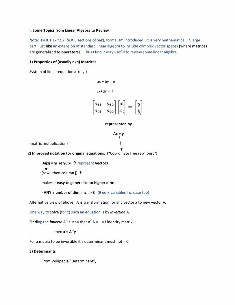
I. Some Topics from Linear Algebra to Review 

Note:  First 1.1‐ ~2.2 (first 8 sections of Sak), formalism introduced.  It is very mathematical, in large 

part, just like an extension of standard linear algebra to include complex vector spaces (where matrices 

are generalized to operators).   Thus I find it very useful to review some linear algebra.    

1) Properties of (usually nxn) Matrices  

System of linear equations:  (e.g.) 

          ax + by = e 

          cx+dy =  f 

 

represented by  

Ax = y                                     

(matrix multiplication) 

2) Improved notation for original equations:  (“Coordinate free rep” best?) 

 Aijxj = yi  ie yi, xi  represent vectors    

(row i then column j) !!! 

makes it easy to generalize to higher dim: 

‐ ANY  number of dim, incl. > 3   (# eq + variables increase too) 

Alternative view of above:  A is transformation for any vector x to new vector y. 

One way to solve (for x) such an equation is by inverting A.   

Finding the inverse A‐1 such= that A‐1A = 1 = I identity matrix 

                          then x = A‐1y 

For a matrix to be invertible it’s determinant must not = 0.     

3) Deterimants 

From Wikipedia “Determinant”,  

“The fundamental geometric meaning of a determinant is a scale factor for measure when A is 

regarded as a linear transformation.”  It is the scale factor for n‐D volumes before and after the 

transformations . 

Property of  Determinant:   det(AB) = det(A)*det(B)  (Easier to compute, e.g. if one has the “LU” 

[Lower/Upper] Decomposition) 

Note oddity:  central to the properties of matrices,   determinant very important in Linear Algebra, 

not ostensibly for QM.  (focus on instead algebraic properties).   

 

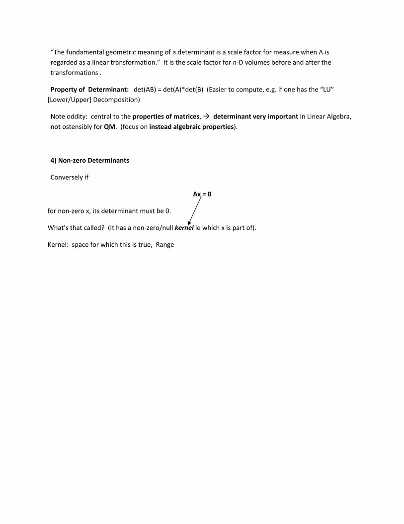
4) Non‐zero Determinants 

Conversely if   

Ax = 0 

for non‐zero x, its determinant must be 0.   

What’s that called?  (It has a non‐zero/null kernel ie which x is part of). 

Kernel:  space for which this is true,  Range  

  

   

Lecture 1/5/10 

Notes uploaded (pages) 

Quiz today (?) 

Reading for tomorrow:  Sakuarai 1.1 

‐‐‐‐‐‐‐‐‐‐‐‐‐‐‐‐‐‐ 

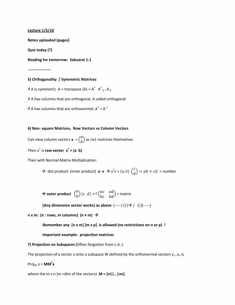
5) Orthogonality  / Symmetric Matrices 

If A is symmetric  A = transpose (A) = AT   AT ij = A ji   

If A has columns that are orthogonal, A called orthogonal 

If A has columns that are orthonormal, AT = A‐1 

 

6) Non‐ square Matrices,  Row Vectors vs Column Vectors 

Can view column vectors x  =   as nx1 matrices themselves  

Then xT is row vector  xT = (a  b) 

Then with Normal Matrix Multiplication:  

  dot product: (inner product)  x∙ v   xTv =        = number 

   

 outer product       ?  = matrix 

 (Any dimension vector works) as above  (‐‐‐‐‐) (|) /   (|)(‐‐‐‐‐) 

n x m:  (n : rows, m columns)  (n ≠ m)     

  ‐Remember any  [n x m] [m x p]  is allowed (no restrictions on n or p)  !    

‐Important example:  projection matrices 

7) Projection on Subspaces (Often forgotten from L.A.:) 

The projection of a vector x onto a subspace W defined by the orthonormal vectors v1..vn is  

ProjW x = MMTx 

where the m x n (m =dim of the vectors)  M = [v1|…|vn].      

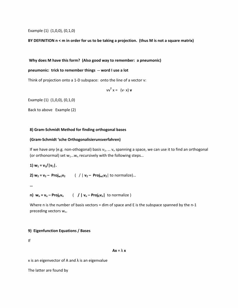
Example (1)  (1,0,0), (0,1,0)   

BY DEFINITION n < m in order for us to be taking a projection.  (thus M is not a square matrix) 

 

 Why does M have this form?  (Also good way to remember:  a pneumonic)   

pneumonic:  trick to remember things  ‐‐ word I use a lot 

Think of projection onto a 1‐D subspace:  onto the line of a vector v: 

vvT x =   (v∙ x) v 

Example (1)  (1,0,0), (0,1,0)   

Back to above   Example (2) 

 

8) Gram‐Schmidt Method for finding orthogonal bases 

(Gram‐Schmidt ‘sche Orthogonalisierunsverfahren) 

If we have any (e.g. non‐othogonal) basis v1, … vn spanning a space, we can use it to find an orthogonal 

(or orthonormal) set w1…wn recursively with the following steps…    

1) w1 = v1/|v1|.    

2) w2 = v2 –  Projw1v2          (   / | v2 –  Projw1v2| to normalize)… 

…  

n)  wn = vn – ProjEvn           (    / | vn – ProjEvn|  to normalize )   

Where n is the number of basis vectors = dim of space and E is the subspace spanned by the n‐1 

preceding vectors wn.  

 

9)  Eigenfunction Equations / Bases 

If  

Ax = λ x 

x is an eigenvector of A and λ is an eigenvalue 

The latter are found by 

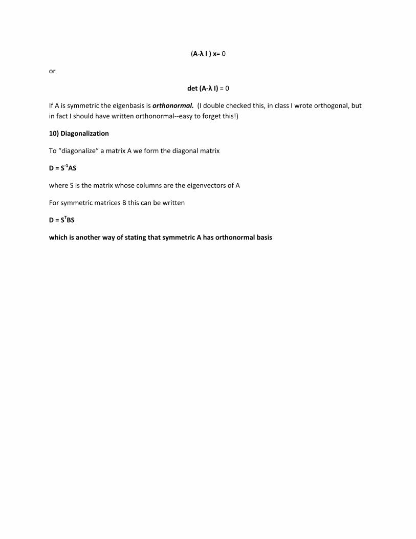
(A‐λ I ) x= 0 

or  

det (A‐λ I) = 0 

If A is symmetric the eigenbasis is orthonormal.  (I double checked this, in class I wrote orthogonal, but 

in fact I should have written orthonormal‐‐easy to forget this!) 

10) Diagonalization 

To “diagonalize” a matrix A we form the diagonal matrix 

D = S‐1AS 

where S is the matrix whose columns are the eigenvectors of A 

For symmetric matrices B this can be written 

D = STBS 

which is another way of stating that symmetric A has orthonormal basis 

   

 

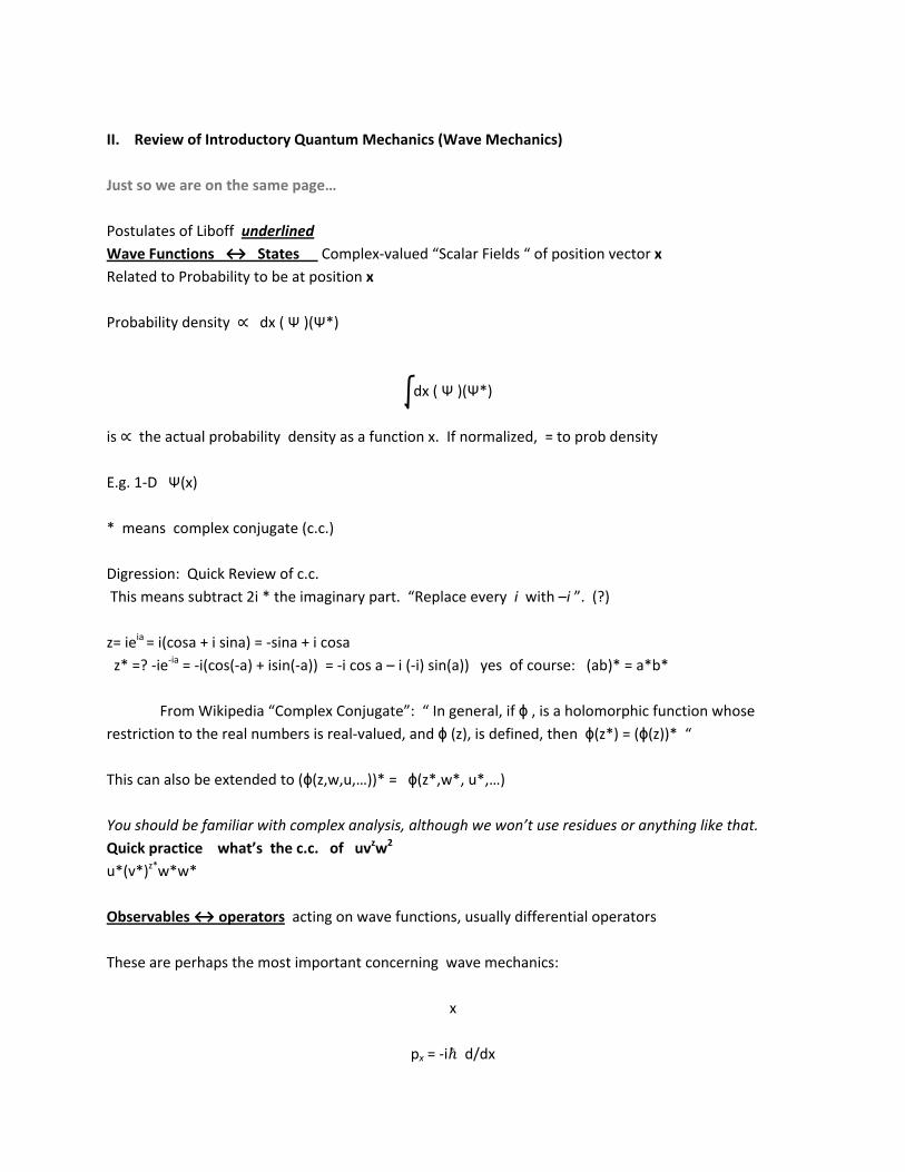
II.    Review of Introductory Quantum Mechanics (Wave Mechanics) 

 

Just so we are on the same page… 

 

Postulates of Liboff  underlined 

Wave Functions   ↔   States      Complex‐valued “Scalar Fields “ of position vector x  

Related to Probability to be at position x 

 

Probability density      dx ( Ψ )(Ψ*)      

 

 

dx ( Ψ )(Ψ*) 

 

is    the actual probability  density as a function x.  If normalized,  = to prob density 

 

E.g. 1‐D   Ψ(x)    

 

*  means  complex conjugate (c.c.) 

 

Digression:  Quick Review of c.c. 

 This means subtract 2i * the imaginary part.  “Replace every  i  with –i ”.  (?)  

 

z= ieia = i(cosa + i sina) = ‐sina + i cosa 

  z* =? ‐ie‐ia = ‐i(cos(‐a) + isin(‐a))  = ‐i cos a – i (‐i) sin(a))   yes  of course:   (ab)* = a*b* 

 

From Wikipedia “Complex Conjugate”:  “ In general, if ϕ , is a holomorphic function whose 

restriction to the real numbers is real‐valued, and ϕ (z), is defined, then  ϕ(z*) = (ϕ(z))*  “ 

 

This can also be extended to (ϕ(z,w,u,…))* =   ϕ(z*,w*, u*,…)   

 

You should be familiar with complex analysis, although we won’t use residues or anything like that. 

Quick practice    what’s  the c.c.   of   uvzw2      

u*(v*)z*w*w* 

 

Observables ↔ operators  acting on wave functions, usually differential operators 

 

These are perhaps the most important concerning  wave mechanics: 

 

x 

 

px = ‐i   d/dx 

 

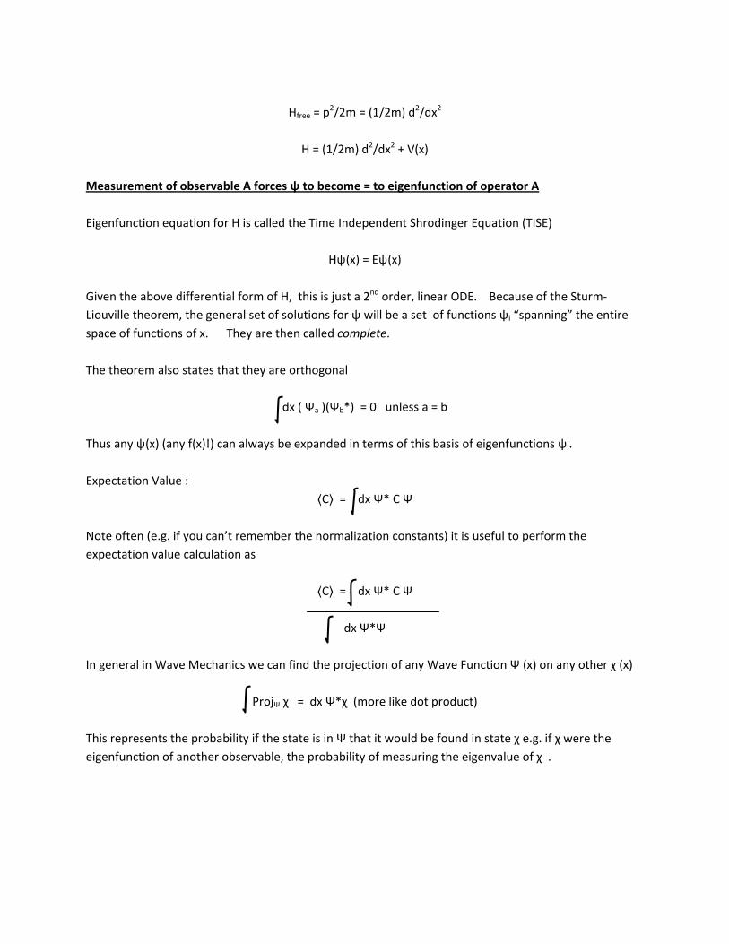
Hfree = p2/2m = (1/2m) d2/dx2 

 

H = (1/2m) d2/dx2 + V(x)  

 

Measurement of observable A forces ψ to become = to eigenfunction of operator A 

 

Eigenfunction equation for H is called the Time Independent Shrodinger Equation (TISE)  

 

Hψ(x) = Eψ(x) 

  

Given the above differential form of H,  this is just a 2nd order, linear ODE.    Because of the Sturm‐

Liouville theorem, the general set of solutions for ψ will be a set  of functions ψi “spanning” the entire 

space of functions of x.      They are then called complete.    

 

The theorem also states that they are orthogonal 

 

dx ( Ψa )(Ψb*)  = 0   unless a = b 

 

Thus any ψ(x) (any f(x)!) can always be expanded in terms of this basis of eigenfunctions ψi.  

 

Expectation Value :  

C   =    dx Ψ* C Ψ 

 

Note often (e.g. if you can’t remember the normalization constants) it is useful to perform the 

expectation value calculation as 

 

C   =    dx Ψ* C Ψ 

 

dx Ψ*Ψ 

 

In general in Wave Mechanics we can find the projection of any Wave Function Ψ (x) on any other χ (x) 

 

ProjΨ χ   =  dx Ψ*χ  (more like dot product) 

 

This represents the probability if the state is in Ψ that it would be found in state χ e.g. if χ were the 

eigenfunction of another observable, the probability of measuring the eigenvalue of χ  . 

 

   

 

 

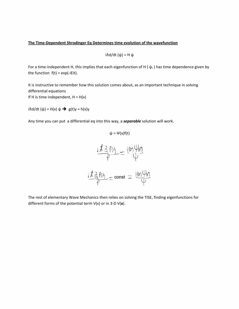
The Time‐Dependent Shrodinger Eq Determines time evolution of the wavefunction 

 

i d/dt (ψ) = H ψ 

 

For a time‐independent H, this implies that each eigenfunction of H ( ψi ) has time dependence given by 

the function  f(t) = exp(‐iEit).   

 

It is instructive to remember how this solution comes about, as an important technique in solving 

differential equations 

If H is time independent, H = H(x) 

 

i d/dt (ψ) = H(x) ψ   g(t)y = h(x)y 

 

Any time you can put  a differential eq into this way, a separable solution will work. 

 

ψ = Ψ(x)f(t) 

 

  

  

The rest of elementary Wave Mechanics then relies on solving the TISE, finding eigenfunctions for 

different forms of the potential term V(x) or in 3‐D V(x).   

 

   

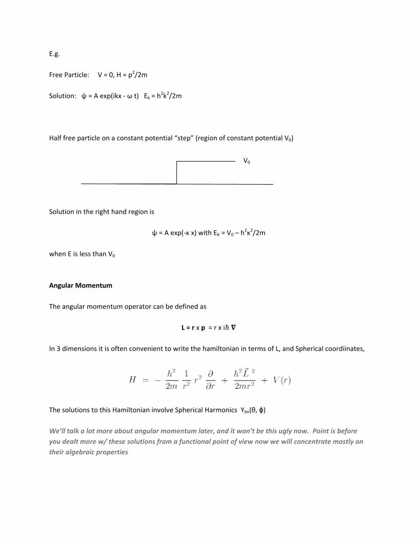
E.g.  

 

Free Particle:     V = 0, H = p2/2m 

 

Solution:   ψ = A exp(ikx ‐ ω t)   Ek = h2k2/2m 

 

 

 

Half free particle on a constant potential “step” (region of constant potential V0) 

 

 

 

 

 

 

Solution in the right hand region is  

 

ψ = A exp(‐κ x) with EK = V0 – h2κ2/2m 

 

when E is less than V0 

 

 

Angular Momentum 

 

The angular momentum operator can be defined as 

 

L = r x p  = r x i    

 

In 3 dimensions it is often convenient to write the hamiltonian in terms of L, and Spherical coordiinates, 

 

  

The solutions to this Hamiltonian involve Spherical Harmonics  Ylm(θ, ϕ) 

 

We’ll talk a lot more about angular momentum later, and it won’t be this ugly now.  Point is before 

you dealt more w/ these solutions from a functional point of view now we will concentrate mostly on 

their algebraic properties 

 

 

 

V0 

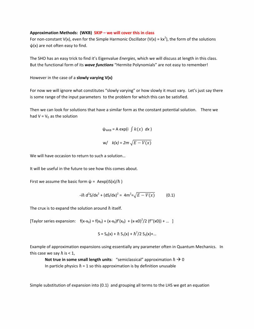
Approximation Methods:  (WKB)  SKIP – we will cover this in class  

For non‐constant V(x), even for the Simple Harmonic Oscillator (V(x) = kx2), the form of the solutions 

ψ(x) are not often easy to find.    

 

The SHO has an easy trick to find it’s Eigenvalue Energies, which we will discuss at length in this class.   

But the functional form of its wave functions “Hermite Polynomials” are not easy to remember! 

   

However in the case of a slowly varying V(x)   

 

For now we will ignore what constitutes “slowly varying” or how slowly it must vary.  Let’s just say there 

is some range of the input parameters  to the problem for which this can be satisfied. 

 

Then we can look for solutions that have a similar form as the constant potential solution.    There we 

had V = V0  as the solution  

 

ψWKB = A exp(i     dx ) 

 

w/    k(x) = 2m   

 

We will have occasion to return to such a solution… 

 

It will be useful in the future to see how this comes about. 

 

First we assume the basic form ψ =  Aexp(iS(x)/  ) 

 

‐i  d2S/dx2 + (dS/dx)2 =  4m2=            (0.1) 

 

The crux is to expand the solution around   itself.    

 

[Taylor series expansion:    f(x‐x0) = f(x0) + (x‐x0)f’(x0)  + (x‐x0)2/2 (f’’(x0)) + …   ]  

 

S = S0(x) +   S1(x) + 2/2 S2(x)+…             

 

Example of approximation expansions using essentially any parameter often in Quantum Mechanics.   In  

this case we say   is < 1,  

Not true in some small length units:   “semiclassical” approximation    0  

In particle physics   = 1 so this approximation is by definition unusable 

 

 

Simple substitution of expansion into (0.1)  and grouping all terms to the LHS we get an equation 

 

F0 +   F1(x) + 2 F2(x) …. = 0  

 

where F0   =  (dS0/dx)2‐4m2 (E‐V(x)) 2 = 0  for example. 

 

The key is that every term in this series must vanish independently.   Thus we can set each term = 0; 

F0 = 0      dS0/dx = k(x)   k given above. 

 

First order simple ODE   And thus we have our solution form. 

 

 

Time Independent Perturbation Theory 

 

Last reminder of Intro QM/Wave Mechanics…  

 

A very similar technique is used for a much more general approximation scheme. 

 

If we can separate H into a form H0 + λ H’ where H0 is one that we know the eigenfunctions for  

 

H’ is called the perturbation () to the Base Hamilitonian. 

 

 

e.g.  the most common thing (e.g. in Quantum Field Theory Scattering Calc’s –note that in that case we 

are talking about a completely different mathematical Hamiltonian.)   is to think of the entire V(x) as a 

“small”   so that H0 in that case is the free particle Hamiltonian.   

 

ie H = p2/2m + V(x)  p2/2m + λ V’(x)    (it would be interesting to see the SHO handled this way—

perhaps we will come back to the idea when we learn about the SHO.) 

 

 

Anyway making a similar expansion to the WKB this time in λ  

 

e.g.      ψ = ϕ0 +λ ϕ1(x) + λ2/2  ϕ2(x) ;       En =  E0 + λ E1+… 

 

And setting each factor of λ n = 0 independently and taking the expectation value of each equation we 

find that we can represent the MODIFICATIONS to the eigenfunctions of H0 in terms of a “mixing” of the 

other eigenfunctions due to the perturbation H’.    

 

        

 

Where mixing is just a projection of one Wave Function Ψi  on another: 

 

   

 

The new Energies (MODIFICATIONS to each states energy) are 

 

Ennew = En

0 + <H’> 

 

 

 

 

   

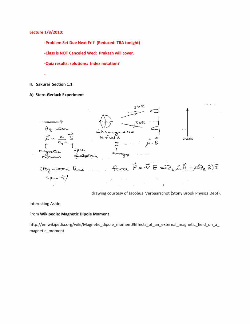
Lecture 1/8/2010: 

‐Problem Set Due Next Fri?  (Reduced: TBA tonight)  

‐Class is NOT Canceled Wed:  Prakash will cover. 

  ‐Quiz results: solutions:  Index notation? 

  ‐ 

II.   Sakurai  Section 1.1 

A)  Stern‐Gerlach Experiment 

 

drawing courtesy of Jacobus  Verbaarschot (Stony Brook Physics Dept). 

Interesting Aside: 

From Wikipedia: Magnetic Dipole Moment 

http://en.wikipedia.org/wiki/Magnetic_dipole_moment#Effects_of_an_external_magnetic_field_on_a_

magnetic_moment 

z‐axis 

 

Interesting idea:  electron (all spin ½ fermions) is composite particle made of two monopoles.  

Analogy:  Fractionally charged quarks confined in proton. 

Two differences from Classical  Expectation     

1) Existence of μ   Spin   :    Sakurai  ‐‐‐‐‐‐ <|)      Liboff:  [ (if unquantized “spin” expected] 

2)   Quantization of  μ    Quantization of Spin (at least in the z  direction)  ‐‐   ‐‐‐__‐‐‐‐__‐‐‐‐ 

Quantization oft spin was  Sz = +/‐   / 2 

  can be determined from the distance btw the 2 peaks  (must have been tiny!)  (probably why no 

lab demonstration) 

   

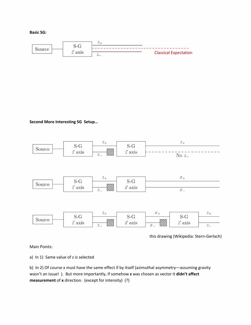
Basic SG:  

 

 

 

 

 

 

Second More Interesting SG  Setup… 

 

 

this drawing (Wikipedia: Stern‐Gerlach) 

Main Points:  

a)  In 1)  Same value of z is selected 

b)  In 2) Of course x must have the same effect if by itself (azimuthal asymmetry—assuming gravity 

wasn’t an issue!  ).  But more importantly, if somehow z was chosen as vector it didn’t affect 

measurement of x direction.  (except for intensity)  (?) 

Classical Expectation 

c) Measurement of x DID affect the outcome of the second z measurement—it made it like the first z 

measurement.  

 

Lecture 1/11/2010 

Pset posted (small changes made Sat)   Index notation reading is optional for this week, but in 

reality required for most 

  Prakash:  Wed: 

 

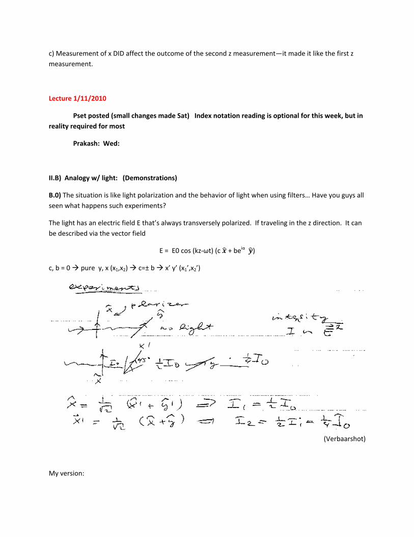
II.B)  Analogy w/ light:   (Demonstrations) 

B.0) The situation is like light polarization and the behavior of light when using filters… Have you guys all 

seen what happens such experiments?   

The light has an electric field E that’s always transversely polarized.  If traveling in the z direction.  It can 

be described via the vector field 

E =  E0 cos (kz‐ωt) (c   + beiα   ) 

c, b = 0  pure  y, x (x1,x2)  c=± b  x’ y’ (x1’,x2’) 

(Verbaarshot) 

 

My version: 

 

 

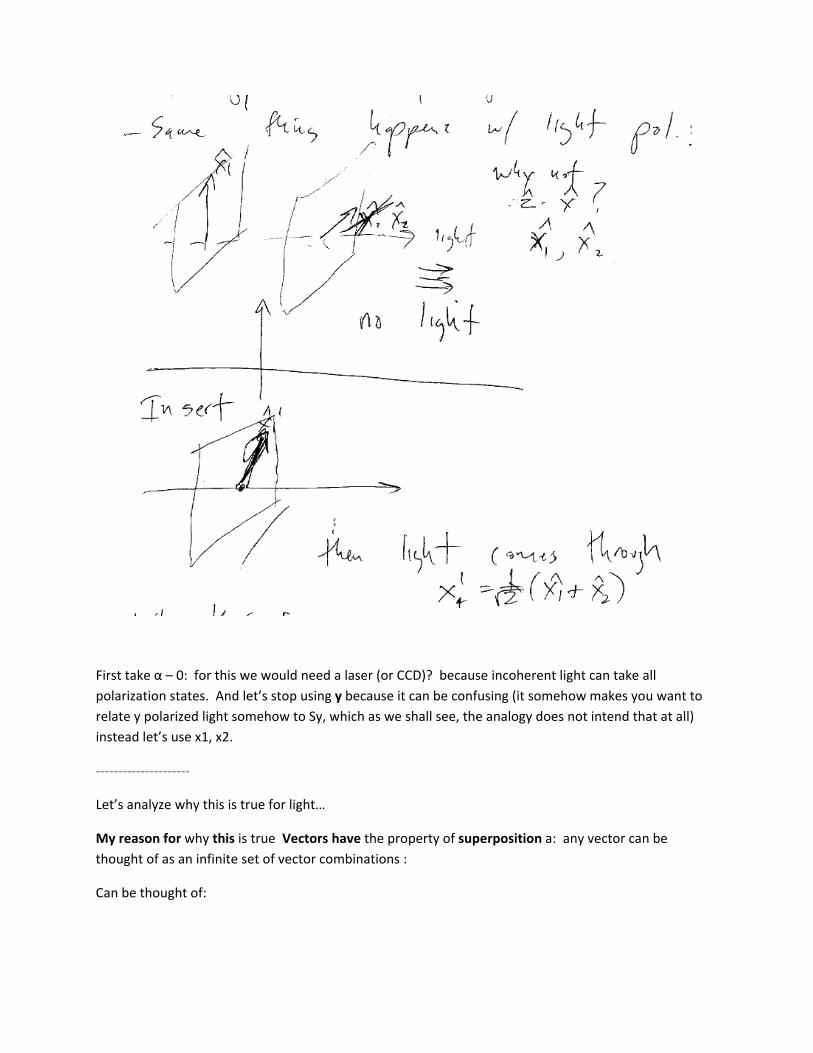
First take α – 0:  for this we would need a laser (or CCD)?  because incoherent light can take all 

polarization states.  And let’s stop using y because it can be confusing (it somehow makes you want to 

relate y polarized light somehow to Sy, which as we shall see, the analogy does not intend that at all)  

instead let’s use x1, x2. 

‐‐‐‐‐‐‐‐‐‐‐‐‐‐‐‐‐‐‐‐‐ 

Let’s analyze why this is true for light… 

My reason for why this is true  Vectors have the property of superposition a:  any vector can be 

thought of as an infinite set of vector combinations :      

Can be thought of:   

 

 

 

 

 

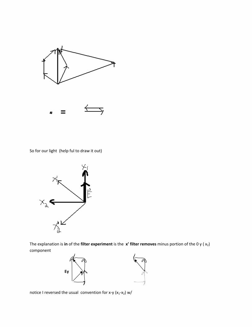
So for our light  (help ful to draw it out)  

 

The explanation is in of the filter experiment is the  x’ filter removes minus portion of the 0 y ( x2) 

component 

 

                                  Ey 

 

notice I reversed the usual  convention for x‐y (x1‐x2) w/   

= 

Weird interpretion :   the electric field Ex  is still “there” in the y‐direction even after x filter, but it just 

has a value of 0.     

 But when we talk about Quantum Mechanical systems, this weird way of looking at it  becomes  “the 

normal way of thinking”. (to think) 

B.1)  QM Explanation of SG 

Thus the idea behind the QM  explanation of the situation of the SG experiment is that the  Ag 

atom’s spin  states re made up of abstract 2‐D vectors called ket’s.   

Denoted w/ ket notation |Sz+> , |Sz‐> 

   

 

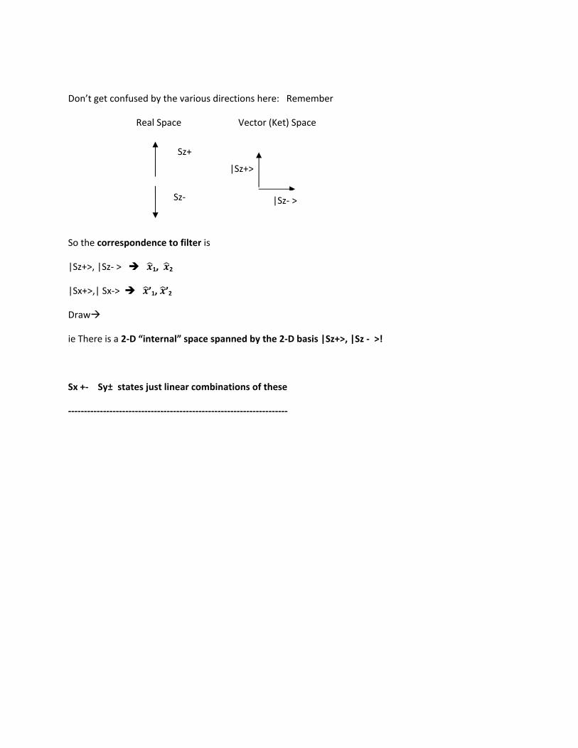
Don’t get confused by the various directions here:   Remember 

                 Real Space    Vector (Ket) Space 

 

 

 

 

So the correspondence to filter is 

|Sz+>, |Sz‐ >       1,   2 

|Sx+>,| Sx‐>      ’1,  ’2 

Draw 

ie There is a 2‐D “internal” space spanned by the 2‐D basis |Sz+>, |Sz ‐  >!  

 

Sx +‐    Sy±  states just linear combinations of these 

‐‐‐‐‐‐‐‐‐‐‐‐‐‐‐‐‐‐‐‐‐‐‐‐‐‐‐‐‐‐‐‐‐‐‐‐‐‐‐‐‐‐‐‐‐‐‐‐‐‐‐‐‐‐‐‐‐‐‐‐‐‐‐‐‐‐‐‐‐ 

   

Sz+ 

Sz‐ 

|Sz+> 

|Sz‐ > 

C)  Important Differences btw SG(QM)/Light 

C.1)  States And Collapse of the “State” 

 A Major difference in interpretation is that for the SG Measurement of Sx  Quantum Mechanics says 

there is a  “Destruction of the State”/”Collapse”     

Difference operationally hard to define now:  Hard to define difference actually‐‐ This can be phrased in 

terms of the “incompatibility of Sz, Sx observables”    

‐Light we can be able to devise an experiment to  “measuring”   ’and xi  components 

simultaneously.     Where as by Quantum Postulate   Sz, Sx cannot be simultaneously measured. 

[Difference operationally hard to define now:]  

For now focus on what is meant by collapse: 

One of the most important points to notice about these experiements, not just that one of 2 values of Sz 

are chosen, but that afterwards the same value is chosen ie state is selected.   (point of “more 

interesting SG Exp…” part (a)  above.   

‐Went from “unpolarized”(isotropic   to “polarized” (Sz)   

called “Collapse of the Wave Function”  

Generalize:  “Collapse of the Wave Function”  Collapse of the State  (now that we aren’t 

doing Wave Mechanics only anymore):   

Postulate:  Measurement causes collapse 

This is something very non‐physical and its nature is still debated.  The major questions about what this 

implies pertain to “Shrodinger’s Cat” type questions—what actually constitutes measurement?.  As Far 

As I Know (AFAIK) they are still unresolved. 

  Copenhagen Interpretation  (this course) measurement causes change, likened 

mathematically to projection operator being applied  

  Many worlds interpretation ‐‐all possibilities are realized ? ( Leonard Suskind:  book) 

  Penrose others: very  non traditional ideas… 

Related to nature of QM entanglement, etc…   To me:  interesting frontier of physics (if experiments can 

be devised)   “Recent” paper claimed measurement position/momentum simultaneously. 

Back to difference w/ light:   Hard to define difference actually—It can be phrased in terms of the 

“incompatibility of Sz, Sx observables”    

‐Light we can be able to devise an experiment to  “measuring”   ’and xi  components 

simultaneously.     Where as by Quantum Postulate   Sz, Sx cannot be simultaneously measured.] 

We will define this more formally later this week… 

 

C.2) (Light Pol/vs QM) Differences btw Polarization/Directions 

The analogy with light is very nice and really helps understand some of the basic ideas of quantum 

mechanics.   But the analogy w/ light can only be taken so far: 

‐Light waves must be transversely polarized.:  Direction of motion matters. 

‐SG:  Direction of particle motion is irrelevant 

These particles do not need to be.  In fact it is easy to mistakenly think that the direction of the particle 

beam is somehow analogous to the direction of the light going through the filter.    In fact the direction 

the particles are moving is somewhat irrelevant.   x and y (Sx, Sy) in the SG are equivalent even though 

one direction is || to the beam and  one is perp.   

So there is No polarization of the SG particles in Real (our Euclidean) 3‐D space.   But they are polarized 

in our “internal”  spin space. 

Mag field defines special direction 

 

C.3)  More Observations about Directions in this Experiment 

This also makes the point that the actual directions themselves  are not so relevant in the SG 

experiment.    Sz was special, quantized, but  Sx (or Sy it turns out—we can do the same experiment with 

the Sy it will be the same) isn’t.    

Mag field defines special direction  NOT beam direction! 

It means that of the three spacial directions, only 1 gets quantized, and the other two are then just 

linear combinations of the quantization.    

So …  

Question:       True/False:   The SG exp. proves that nature has a preferred direction (z)?    A: False 

BUT:                True/False:    The SG exp. proves that nature prefers ONE direction ?              A:  True 

 –it does prefer ONE direction out of the 3 directions inherent in 3‐D space, considering the Ang 

Momentum of Quantum Particles.  For any given particle locally 3 space? 

How about if we define an axis z before the experiment‐‐before it’s measured what is its spin state?—

Can’t we define it in terms of this axis?   Yes , this chapter instructs us that we can—regardless of 

whether we put a SG magnetic field there or not in fact.  But of course that still doesn’t imply that our 

chosen z direction itself is preferred—rather just that ONE direction is preferred. 

IE  Better to think more abstractly here:   The major point of these experiments is that there is ONE 

special  space axis   not necessary that we call it z,  but still there is 1.   It’s probably best (though not 

required) to call it the  “ALIGNED” axis, meaning aligned w/ the magnetic field.  

In fact, the experiments imply not just that ALIGNED is special, but that there are 2 special space 

directions.    ALIGNED and ANTI‐ALIGNED.   

Correspondingly the other 2 space axes/ 4 spacial directions w.r.t. these two directions have hardly any 

special significance, they are just linear combinations of the first 2‼‼    In the internal spin space, the fact 

that in real space, those other directions/axes correspond to linearly independent vectors/axes is 

irrelevant. 

We shall see that Quantum Mechanics is constructed in a way that automatically causes this weird 

situation to have a mathematical explanation.   

 

B.5)   The role of Sy in Sakarai 1.1:  

Finally  we haven’t talked to much about Sy.     

Sakurai’s point is that treating Sy REQUIRES us to use complex spaces.     

That we can continue our analogy w/ Sy  by simply choosing the circularly polarized state with  

β = 1 ,  α = +/‐ π /2 

E =  E0 cos (kz‐ωt) ( + eiα   ) 

Ie  

E =  E0 cos (kz‐ωt)  + E0 sin(kz‐ωt)    

 

This is very nice:    it makes the analogy so much nicer and very natural.    

 

 

 

Just to summarize the whole analogy now: 

 

|Sz+>, |Sz‐ >       1,  2 

|Sx+>,| Sx‐>      ’1,  ’2        w/  real coefficients (e.g. α = 0)  

|Sy+>,| Sy‐>      ’1,  ’2         w/ complex phase (α = ± π/2)  

Sx:  b = ±  c would give x’ considered so far (45) but other combo’s will be considered in homework 

problems.   

Important point again:   |Sy+>  is not orthogonal to |Sx+>:  just one is complex one is not 

However in the end there IS one thing special about Sx and Sy in relation to Sz:  they are “maximally 

incompatible” with z and with each other.  Perpendicular in real space maps to maximal destruction of 

one chosen direction by measurement of the perp dir. 

‐‐‐‐‐‐‐‐‐‐‐‐‐‐‐‐‐‐‐‐‐‐‐‐‐‐‐‐‐‐‐‐‐‐‐‐‐‐‐‐‐ 

However, I pondered whether it was true—could we use some other mathematical device, perhaps 

higher dimensional matrices, for our initial state vectors and avoid complex numbers.    The answer is 

yes, but it would be very complicated. 

One way to see this before even approaching our SG, is to start with answer the following more simple 

question.   Complex numbers are much like 2‐D vectors.  Can we actually define an algebra using 2‐D 

vectors that have all the properties of complex numbers.    Let me show you one I thought of—it’s good 

practice w/ complex numbers and also an example of thinking about “constructing” algebras that fulfill 

your needs, something that is done in advanced physics all the time (e.g. dot product in General 

Relativity defined w/ metric—String Theory, etc…) :    

The idea is to take our  z = a+bi            

actually this way requires a special definition of “inner product” like in relativity one needs a “metric” to 

put in the minus sign (remember only dealing w/ real numbers) 

Actually Wikipedia shows us a better way… 

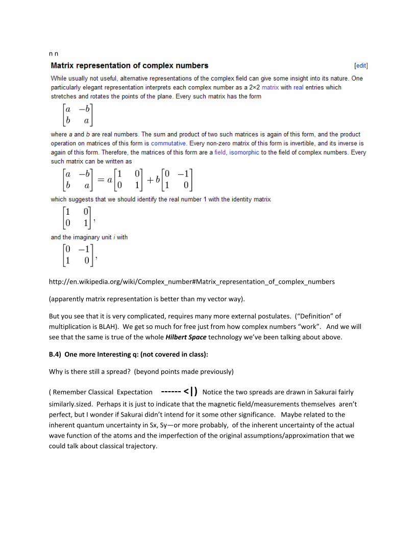
n n 

 

http://en.wikipedia.org/wiki/Complex_number#Matrix_representation_of_complex_numbers 

(apparently matrix representation is better than my vector way). 

But you see that it is very complicated, requires many more external postulates.  (“Definition” of 

multiplication is BLAH).  We get so much for free just from how complex numbers “work”.   And we will 

see that the same is true of the whole Hilbert Space technology we’ve been talking about above. 

B.4)  One more Interesting q: (not covered in class):  

Why is there still a spread?  (beyond points made previously) 

( Remember Classical  Expectation     ‐‐‐‐‐‐ <|)  Notice the two spreads are drawn in Sakurai fairly similarly.sized.  Perhaps it is just to indicate that the magnetic field/measurements themselves  aren’t 

perfect, but I wonder if Sakurai didn’t intend for it some other significance.   Maybe related to the 

inherent quantum uncertainty in Sx, Sy—or more probably,  of the inherent uncertainty of the actual 

wave function of the atoms and the imperfection of the original assumptions/approximation that we 

could talk about classical trajectory.   

 

   

Lecture 1/12/2010 

For problem 1.2:  just view σi as being complex matrices with the following definitions 

         

   : Vector of Matrices 

For problem 1.12:  can use the result of 1.9 without proof. 

IMPORTANT:  I WILL UPDATE THESE NOTES IN EVENING OF 1/12 to better reflect what we 

covered and what we skipped. 

III.  Quantum Formulism 1:   Abstract Vector or Hilbert Spaces 

A) Hilbert Space 

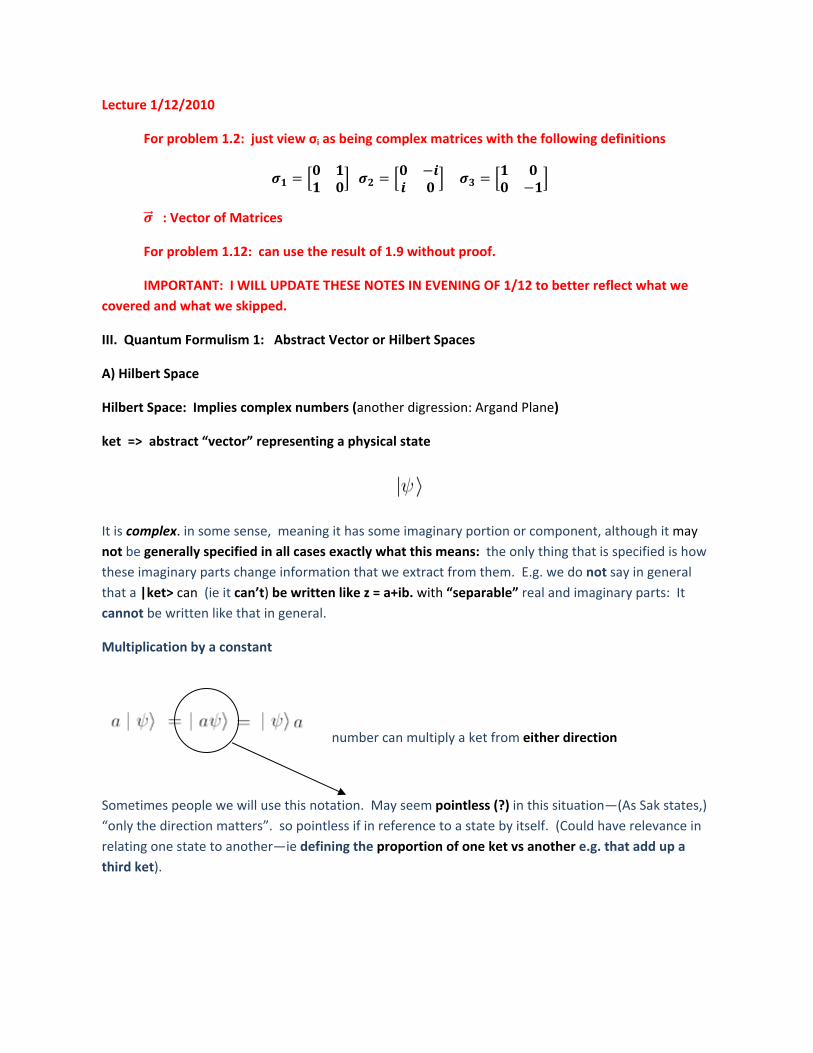
Hilbert Space:  Implies complex numbers (another digression: Argand Plane) 

ket  =>  abstract “vector” representing a physical state 

 

It is complex. in some sense,  meaning it has some imaginary portion or component, although it may 

not be generally specified in all cases exactly what this means:  the only thing that is specified is how 

these imaginary parts change information that we extract from them.  E.g. we do not say in general 

that a |ket> can  (ie it can’t) be written like z = a+ib. with “separable” real and imaginary parts:  It  

cannot be written like that in general. 

Multiplication by a constant 

 

  number can multiply a ket from either direction 

 

Sometimes people we will use this notation.  May seem pointless (?) in this situation—(As Sak states,)  

“only the direction matters”.  so pointless if in reference to a state by itself.  (Could have relevance in 

relating one state to another—ie defining the proportion of one ket vs another e.g. that add up a 

third ket).     

 

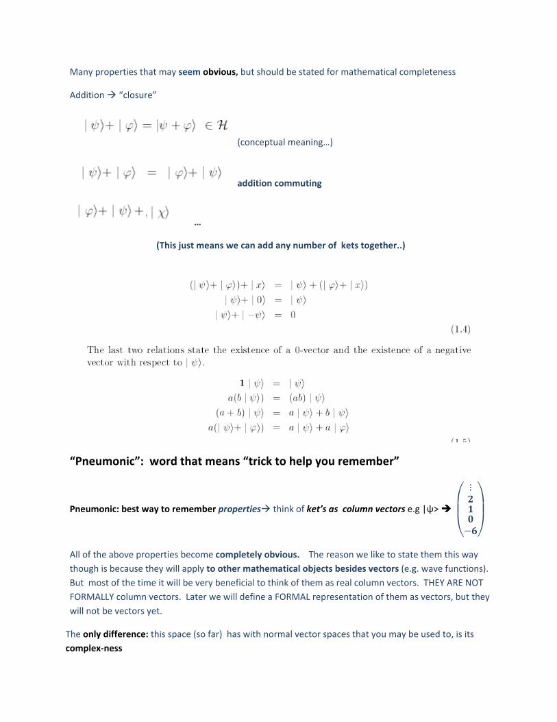
Many properties that may seem obvious, but should be stated for mathematical completeness 

Addition  “closure” 

 (conceptual meaning…) 

 addition commuting 

… 

(This just means we can add any number of  kets together..) 

 

“Pneumonic”:  word that means “trick to help you remember” 

Pneumonic: best way to remember properties think of ket’s as  column vectors e.g |ψ>     

All of the above properties become completely obvious.    The reason we like to state them this way 

though is because they will apply to other mathematical objects besides vectors (e.g. wave functions).  

But  most of the time it will be very beneficial to think of them as real column vectors.  THEY ARE NOT 

FORMALLY column vectors.  Later we will define a FORMAL representation of them as vectors, but they 

will not be vectors yet. 

The only difference: this space (so far)  has with normal vector spaces that you may be used to, is its 

complex‐ness 

   

It is perfectly acceptable:  in a Hilbert Space for any of the above constant factors (numbers multiplying) 

kets to be complex 

 

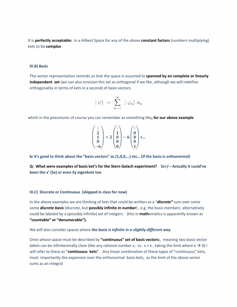
III.B) Basis 

The vector representation reminds us that the space is assumed to spanned by an complete or linearly 

independent  set (we can also envision this set as orthogonal if we like, although we will redefine 

orthogonality in terms of kets in a second) of basis vectors. 

 

which in the pneumonic of course you can remember as something like, for our above example 

 +… 

ie it’s good to think about the “basis vectors” as (1,0,0,…) etc… (if the basis is orthonormal) 

Q:  What were examples of basis ket’s for the Stern Gelach experiment?    Sz+/‐‐‐Actually it could’ve 

been the x’ (Sx) or even Sy eigenkets too 

 

III.C)  Discrete or Continuous  (skipped in class for now) 

In the above examples we are thinking of kets that could be written as a “discrete” sum over some 

some discrete basis (discrete, but possibly infinite in number) , e.g. the basis members  alternatively 

could be labeled by a (possibly infinite) set of integers.   (this in mathematics is apparently known as 

“countable” or “denumerable”). 

We will also consider spaces where the basis is infinite in a slightly different way   

Ones whose space must be described by “continuous” set of basis vectors:,  meaning two basis vector 

labels can be infinitesimally close (like any rational number x,  vs.  x + ϵ , taking the limit where ϵ  0) I 

will refer to these as “continuous  kets”.   Any linear combination of these types of “continuous” kets, 

most  importantly the expansion over the orthonormal  basis kets,  as the limit of the above vector 

sums as an integral 

    

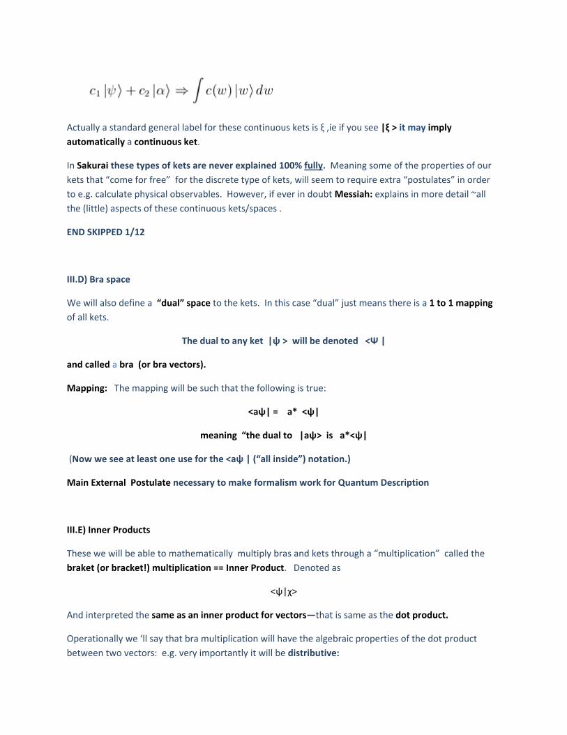
Actually a standard general label for these continuous kets is ξ ,ie if you see |ξ > it may imply 

automatically a continuous ket. 

In Sakurai these types of kets are never explained 100% fully.  Meaning some of the properties of our 

kets that “come for free”  for the discrete type of kets, will seem to require extra “postulates” in order 

to e.g. calculate physical observables.  However, if ever in doubt Messiah: explains in more detail ~all 

the (little) aspects of these continuous kets/spaces . 

END SKIPPED 1/12 

 

III.D) Bra space 

We will also define a  “dual” space to the kets.  In this case “dual” just means there is a 1 to 1 mapping 

of all kets. 

The dual to any ket  |ψ >  will be denoted   <Ψ | 

and called a bra  (or bra vectors). 

Mapping:   The mapping will be such that the following is true: 

<aψ| =    a*  <ψ|  

meaning  “the dual to   |aψ>  is   a*<ψ|   

 (Now we see at least one use for the <aψ | (“all inside”) notation.) 

Main External  Postulate necessary to make formalism work for Quantum Description 

 

III.E) Inner Products 

These we will be able to mathematically  multiply bras and kets through a “multiplication”  called the 

braket (or bracket!) multiplication == Inner Product.   Denoted as 

<ψ|χ> 

And interpreted the same as an inner product for vectors—that is same as the dot product. 

Operationally we ‘ll say that bra multiplication will have the algebraic properties of the dot product 

between two vectors:  e.g. very importantly it will be distributive: 

<ψ|χ+ϕ> = <ψ|χ> + <ψ|ϕ> 

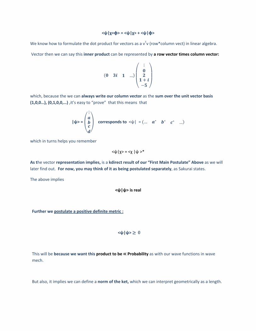
We know how to formulate the dot product for vectors as a vTv (row*column vect) in linear algebra. 

 Vector then we can say this inner product can be represented by a row vector times column vector: 

…  

which, because the we can always write our column vector as the sum over the unit vector basis 

(1,0,0…), (0,1,0,0,…) ,it’s easy to “prove”  that this means  that 

|ψ> =      corresponds to  <ψ|  =  … …  

which in turns helps you remember  

<ψ|χ> = <χ |ψ >* 

As the vector representation implies, is a kdirect result of our “First Main Postulate” Above as we will 

later find out.  For now, you may think of it as being postulated separately, as Sakurai states. 

The above implies    

<ψ|ψ> is real 

 

Further we postulate a positive definite metric :   

 

<ψ|ψ>    0 

 

This will be because we want this product to be   Probability as with our wave functions in wave 

mech. 

 

But also, it implies we can define a norm of the ket, which we can interpret geometrically as a length. 

 

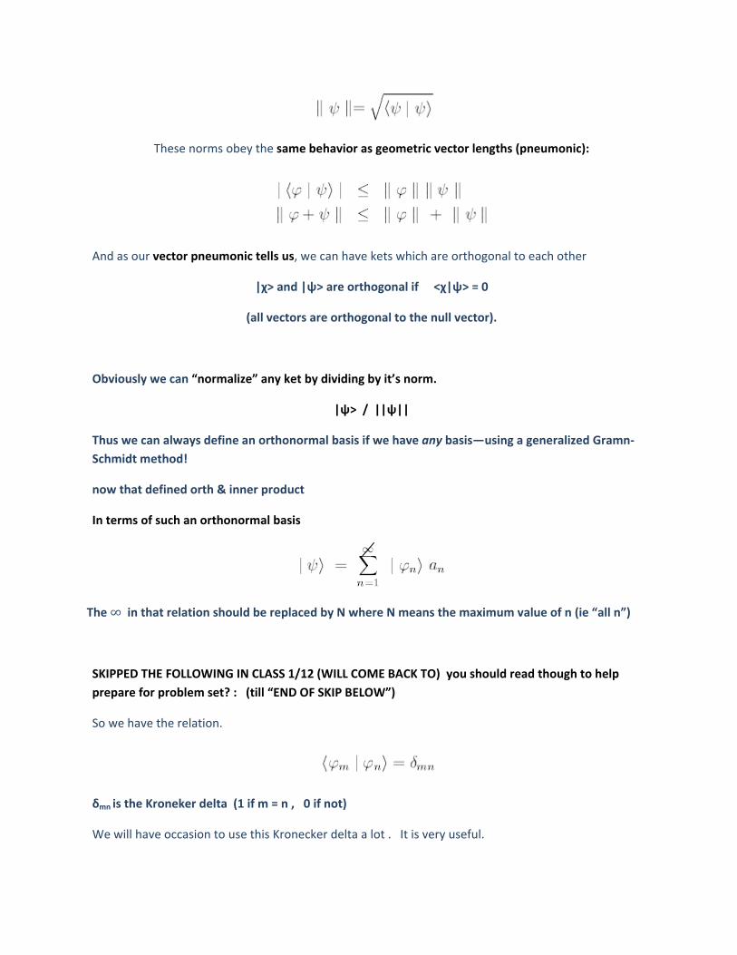
These norms obey the same behavior as geometric vector lengths (pneumonic): 

 

And as our vector pneumonic tells us, we can have kets which are orthogonal to each other 

|χ> and |ψ> are orthogonal if     <χ|ψ> = 0 

(all vectors are orthogonal to the null vector). 

 

Obviously we can “normalize” any ket by dividing by it’s norm.   

|ψ>  /  ||ψ||   

Thus we can always define an orthonormal basis if we have any basis—using a generalized Gramn‐

Schmidt method! 

now that defined orth & inner product 

In terms of such an orthonormal basis 

 

The ∞  in that relation should be replaced by N where N means the maximum value of n (ie “all n”) 

 

SKIPPED THE FOLLOWING IN CLASS 1/12 (WILL COME BACK TO)  you should read though to help 

prepare for problem set? :   (till “END OF SKIP BELOW”) 

So we have the relation.   

 

δmn is the Kroneker delta  (1 if m = n ,   0 if not) 

We will have occasion to use this Kronecker delta a lot .   It is very useful.      

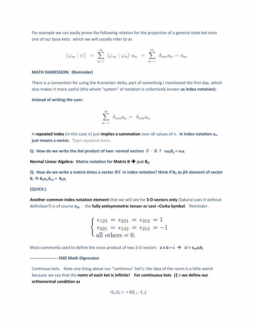
For example we can easily prove the following relation for the projection of a general state ket onto 

one of our base kets:  which we will usually refer to as  

 

MATH DIGRESSION:  (Reminder) 

There is a convention for using the Kronecker delta, part of something I mentioned the first day, which 

also makes it more useful (this whole “system” of notation is collectively known as index notation): 

Instead of writing the sum: 

 

A repeated index (in this case n) just implies a summation over all values of n.  In index notation am 

just means a vector.  Type equation here. 

Q:  How do we write the dot product of two∙ normal vectors     ·     ?   viujδij = viui 

Normal Linear Algebra:  Matrix notation for Matrix B  just Bij. 

Q:  How do we write a matrix times a vector    in index notation? think if Bij as jth element of vector 

Bi  Bijxmδmj =  Bijxj 

(QUICK:) 

Another common index notation element that we will see for 3‐D vectors only (Sakarai uses it without 

definition?) is of course ϵijk  :  the fully antisymmetric tensor or Levi –Civita Symbol.   Reminder: 

 

Most commonly used to define the cross product of two 3‐D vectors   a x b = c     ci = ϵijkaibj 

‐‐‐‐‐‐‐‐‐‐‐‐‐‐‐‐‐‐‐‐ END Math Digression 

Continous kets.   Note one thing about our “continous” ket’s: the idea of the norm is a little weird 

because we say that the norm of each ket is infinite!    For continuous kets  |ξ > we define our 

orthonormal condition as  

<ξ1|ξ2 >  = δ(ξ 1 ‐ ξ 2) 

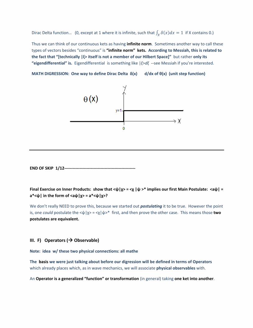
Dirac Delta function…   (0, except at 1 where it is infinite, such that  1  if X contains 0.) 

Thus we can think of our continuous kets as having infinite norm.  Sometimes another way to call these 

types of vectors besides “continuous” is “infinite norm”  kets.  According to Messiah, this is related to 

the fact that “[technically |ξ> itself is not a member of our Hilbert Space]”  but rather only its 

“eigendifferential” is.  Eigendifferential  is something like |ξ>dξ  ‐‐see Messiah if you’re interested. 

MATH DIGRESSION:  One way to define Dirac Delta  δ(x)       d/dx of θ(x)  (unit step function) 

 

 

 

END OF SKIP  1/12‐‐‐‐‐‐‐‐‐‐‐‐‐‐‐‐‐‐‐‐‐‐‐‐‐‐‐‐‐‐‐‐‐‐‐‐‐‐‐‐‐‐‐‐‐‐‐‐‐‐‐ 

 

Final Exercise on Inner Products:  show that <ψ|χ> = <χ |ψ >* implies our first Main Postulate:  <aψ| = 

a*<ψ| in the form of <aψ|χ> = a*<ψ|χ>?  

We don’t really NEED to prove this, because we started out postulating it to be true.  However the point 

is, one could postulate the <ψ|χ> = <χ|ψ>*  first, and then prove the other case.  This means those two 

postulates are equivalent. 

 

III.  F)   Operators ( Observable) 

Note:  idea  w/ these two physical connections: all mathe 

The  basis we were just talking about before our digression will be defined in terms of Operators 

which already places which, as in wave mechanics, we will associate physical observables with.  

An Operator is a generalized “function” or transformation (in general) taking one ket into another.   

 

 

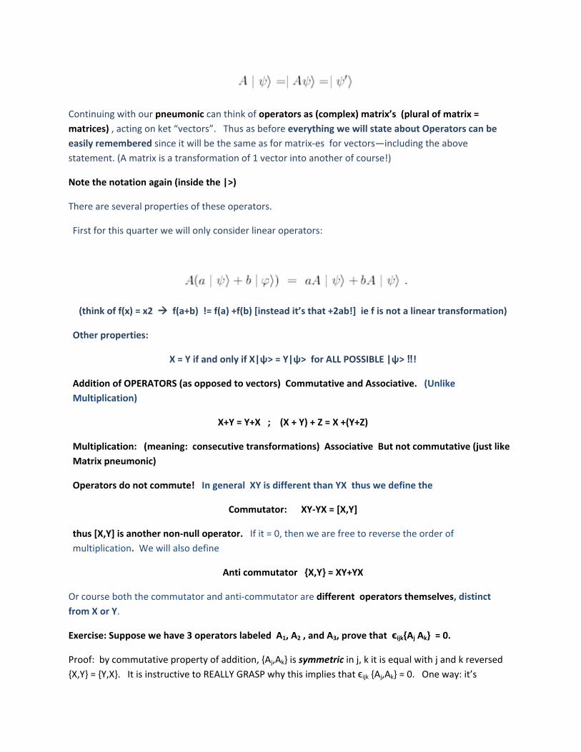
Continuing with our pneumonic can think of operators as (complex) matrix’s  (plural of matrix = 

matrices) , acting on ket “vectors”.   Thus as before everything we will state about Operators can be 

easily remembered since it will be the same as for matrix‐es  for vectors—including the above 

statement. (A matrix is a transformation of 1 vector into another of course!) 

Note the notation again (inside the |>) 

There are several properties of these operators. 

First for this quarter we will only consider linear operators: 

 

 

(think of f(x) = x2    f(a+b)  != f(a) +f(b) [instead it’s that +2ab!]  ie f is not a linear transformation) 

Other properties: 

X = Y if and only if X|ψ> = Y|ψ>  for ALL POSSIBLE |ψ> ‼! 

Addition of OPERATORS (as opposed to vectors)  Commutative and Associative.   (Unlike 

Multiplication) 

X+Y = Y+X   ;    (X + Y) + Z = X +(Y+Z) 

Multiplication:   (meaning:  consecutive transformations)  Associative  But not commutative (just like 

Matrix pneumonic) 

Operators do not commute!   In general  XY is different than YX  thus we define the 

Commutator:      XY‐YX = [X,Y] 

thus [X,Y] is another non‐null operator.   If it = 0, then we are free to reverse the order of 

multiplication.  We will also define 

Anti commutator   {X,Y} = XY+YX 

Or course both the commutator and anti‐commutator are different  operators themselves, distinct 

from X or Y. 

Exercise: Suppose we have 3 operators labeled  A1, A2 , and A3, prove that  ϵijk{Aj Ak}  = 0.  

Proof:  by commutative property of addition, {Aj,Ak} is symmetric in j, k it is equal with j and k reversed 

{X,Y} = {Y,X}.   It is instructive to REALLY GRASP why this implies that ϵijk {Aj,Ak} = 0.   One way: it’s 

because for each value of i, ϵijk{Aj,Ak} is a sum over nine terms which are 9 different anti‐commutators.  

First, by definition of ϵ, the 3 terms that have j = k are automatically 0.  For each of the 6 remaining 

terms  we can match them up and create 3 pairs, each of which as the same two indices, but in reversed 

order  e.g. one term will be ϵi12{A1,A2}  1‐2, the other will have 2‐1 ‐‐ ϵi21{ A2,A1} .  Since {A1,A2} = {A2,A1} 

these two terms are obvious equal but due the ϵ having reversed indicies, opposite in sign and therefore 

each pair adds to 0. 

Better way: (?)   by our j,k  symmetry due to commutativity of addition, ϵijk{Aj,Ak} = ϵijk{Ak,Aj} .   We are 

free to choose any letters for our indices, so obviously on the RHS we can re‐name the indices j→k , kj.  

Then it becomes manifestly obvious that the RHS = ‐(LHS)   (still 9  6 term sums, but each non‐zero 

term will obviously always get the opposite sign.   The only number (besides possibly infinity sometimes 

perhaps) that = the negative of itself is 0. 

Identity operator    or  .  (special operator) This is defined as the operator whose transformation 

doesn’t change a ket at all.  1|ψ> = 1|ψ>.  The same as multiplying by a constant 1, however a true 

operator.  (Like the identity matrix, which has the same effect, but is different from  the number 1)  

Inverse:  Operators can have one:   if they multiply together to make the identity operator 

AB = 1 

then B = A‐1  and we call B and A‐1 the inverse of A.  For a product of operators. 

(AB)‐1 = B‐1A‐1 

This follows from thinking of the operators as transformations. 

Exercise:   Explain this (what I mean) 

(matrix  (AB)‐1 = B‐1A‐1   also—pneumonic)  

However, operators do not ALWAYS have an inverse (just like all matrices don’t). 

Example of an operator:  An interesting “more explicit” operator: “ outer product”:   

 

 

SKIPPED 1/12:   (to “END OF SKIP”): ‐‐‐‐‐‐‐‐‐‐‐‐‐‐‐‐‐‐‐‐‐‐‐ 

There is a basic form of an operator that can be made purely in terms of kets/bras.  It is called the outer 

product. 

|ψ><χ| 

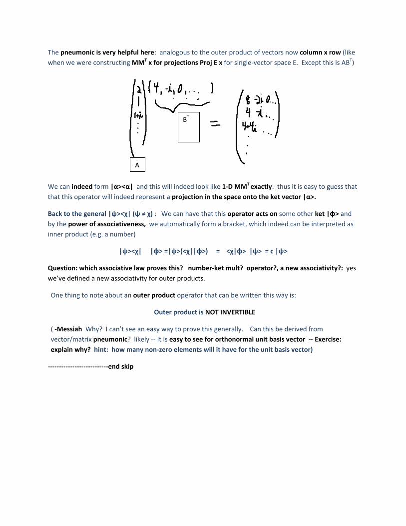
The pneumonic is very helpful here:  analogous to the outer product of vectors now column x row (like 

when we were constructing MMT x for projections Proj E x for single‐vector space E.  Except this is ABT) 

 

We can indeed form |α><α|  and this will indeed look like 1‐D MMT exactly:  thus it is easy to guess that 

that this operator will indeed represent a projection in the space onto the ket vector |α>.   

Back to the general |ψ><χ| (ψ ≠ χ) :   We can have that this operator acts on some other ket |ϕ> and 

by the power of associativeness,  we automatically form a bracket, which indeed can be interpreted as 

inner product (e.g. a number) 

|ψ><χ|     |ϕ> =|ψ>(<χ||ϕ>)     =    <χ|ϕ>  |ψ>  = c |ψ> 

Question: which associative law proves this?   number‐ket mult?  operator?, a new associativity?:  yes 

we’ve defined a new associativity for outer products. 

One thing to note about an outer product operator that can be written this way is: 

Outer product is NOT INVERTIBLE 

( ‐Messiah  Why?  I can’t see an easy way to prove this generally.    Can this be derived from 

vector/matrix pneumonic?  likely ‐‐ It is easy to see for orthonormal unit basis vector  ‐‐ Exercise:  

explain why?  hint:  how many non‐zero elements will it have for the unit basis vector) 

‐‐‐‐‐‐‐‐‐‐‐‐‐‐‐‐‐‐‐‐‐‐‐‐‐‐‐end skip 

 

   

BT

A 

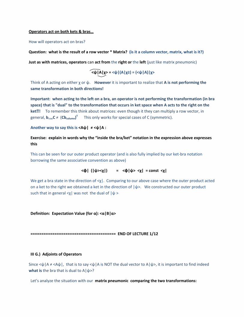
Operators act on both kets & bras…  

How will operators act on bras? 

Question:  what is the result of a row vector * Matrix?  (is it a column vector, matrix, what is it?) 

Just as with matrices, operators can act from the right or the left (just like matrix pneumonic) 

<ψ|A|χ> = <ψ|(A|χ≥) = (<ψ|A)|χ> 

Think of A acting on either χ or ψ.    However it is important to realize that A is not performing the 

same transformation in both directions! 

Important:  when acting to the left on a bra, an operator is not performing the transformation (in bra 

space) that is "dual" to the transformation that occurs in ket space when A acts to the right on the 

ket‼!     To remember this think about matrices: even though it they can multiply a row vector, in 

general, browC ≠  (Cbcolumn)T       This only works for special cases of C (symmetric). 

Another way to say this is <Aψ|  ≠ <ψ|A :  

Exercise:  explain in words why the “inside the bra/ket” notation in the expression above expresses 

this 

This can be seen for our outer product operator (and is also fully implied by our ket‐bra notation 

borrowing the same associative convention as above) 

    <ϕ|  (|ψ><χ|)         =    <ϕ|ψ>  <χ|  = const  <χ| 

We get a bra state in the direction of <χ|.  Comparing to our above case where the outer product acted 

on a ket to the right we obtained a ket in the direction of |ψ>.   We constructed our outer product  

such that in general <χ| was not  the dual of |ψ > 

 

Definition:  Expectation Value (for α): <α|B|α> 

 

=======================================  END OF LECTURE 1/12 

 

III G.)  Adjoints of Operators 

Since <ψ|A ≠ <Aψ|,  that is to say <ψ|A is NOT the dual vector to A|ψ>, it is important to find indeed 

what is the bra that is dual to A|ψ>?    

Let’s analyze the situation with our  matrix pneumonic  comparing the two transformations: 

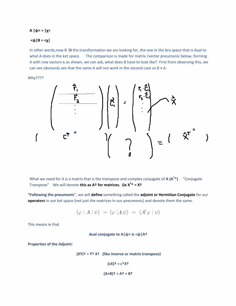
A |ψ> = |χ>    

 <ψ|B = <χ| 

In other words,now B  IS the transformation we are looking for, the one in the bra space that is dual to 

what A does in the ket space.      The comparison is made for matrix /vector pneumonic below, forming 

A with row vectors ri as shown, we can ask, what does B have to look like?  First from observing this, we 

can see obviously see that the same A will not work in the second case so B ≠ A.   

Why???? 

 

What we need for A is a matrix that is the transpose and complex conjugate of A (AT*) .   “Conjugate 

Transpose”    We will denote this as A† for matrices.  (ie XT* = X†  

“Following the pneumonic”, we will define something called the adjoint or Hermitian Conjugate for our  

operators in our ket space (not just the matrices in our pneumonic) and denote them the same. 

 

This means ie that  

dual conjugate to A|ψ> is <ψ|A†  

Properties of the Adjoint: 

 (XY)† = Y† X†   (like inverse or matrix transpose) 

(cX)† = c*X† 

(A+B)† = A† + B† 

** 

same as  T* for matrices.   Easy to forget last one—exercise –“prove w/ our pneumonic”?    Good 

practice for index notation   we add the matrix together element by element:  (A+B)ij = Aij + Bij       

Because of our complex conjugate rule * applies to each term in the equation.   To perform the 

Transpose, in index notation, we simply reverse the order of the indices, so taking the transpose of the 

LHS we get ((A+B)*)ji   but  by the element by element logic, this is just Aji*+Bji *.   which is A† + B†  

 

Finally based on the definitions, multiplications, etc…,  outlined above one property of thing about our 

special outer product operator is  

((|ψ><χ|)† =      |χ><ψ| 

Why?   Apply |ψ><χ|  to |ϕ> : we get c|ψ> where c = <χ|ϕ>.    By our rules, the dual to c|ψ> is <ψ|c* = 

c*<ψ|.   But c* can  obviously be written as <ϕ|χ >, since c = <χ|ϕ>.   So the dual c*|ψ> can be written 

<ϕ|χ><ψ| .   

Question:  what is a special about our projection operator |α><α| with respect to the Adjoint?  it is 

the adjoint of itself!  We have a name for such operators… 

III.H)  Hermitian Operators 

An operator is A called self adjoint  or most of time also Hermitian if 

A = A† 

We will require that the operators we want to represent observables will be Hermitian in Quantum 

Mechanics, for reasons we will soon see.   Apparently there is a slight conceptual difference between 

being Hermitian and being self‐adjoint.    The technical definition of Hermitian:  H is Hermitian if 

<Hψ|ψ>   =  <ψ|Hψ> 

For this class we will refer to Hermitian and self‐adjoint as meaning exactly the same thing: A=A†  

 

 

Exercise:   If A and B are Hermitian (Self Adjoint) is the product AB?  only if they commute 

(AB)†  = B† A† = BA 

III.J)     Eigenkets/Eigenstates 

Following the example of wave mechanics, you knew we were going to have eigen‐somethings… 

If we have the following relation 

|         |   

then we call the ket |β> the eigenket  of the operator A.    We will sometimes follow the convention in 

Sakarai and label our eigenstates by their eigenvalue (which assumes that there are no degeneracies)   

Eigenvalue degeneracy :  means two or more linearly independent eigenkets correspond to the same 

eigenvalue 

Actually the notation we have been using for basis kets | n> is nice because it avoids this issue—let’s 

use a combination of both   B|bn> ‐= bn| bn> .    Sakarai’s notation has a problem of needing multiple 

primes as we will soon see...this is a much nicer convention than using multiple primes (e.g. a’’’).  

Hermitian Operator has real eigenvalues:  important proof 

First notice that even if |β> is an eigenket of B,  if B is NOT Hermitian, then <β| might NOT be an 

eigenbra of B.    It is only the eigenbra of B†.    The eigenvalue for B†  in bra space is must be b* for how 

we defined the dual space.   So the relation corresponding to eq III.1 is 

<β|b* = <β|B† 

 

For a Hermitian operator B , this of course becomes 

<β|b* = <β|B 

 

Now that this is established let’s switch to our new eigenvalue notation and go over the proof in Sakarai 

that the eigenvalues for such a Hermitian B must be real.  Consider when B is bracketed by two different 

eigenstates:    <bn|B|bm> :  operating in either direction with b we see that 

<bn|B|bm> = <bn|bn*|bm> = <bn|bm|bm> 

considering the two right hand quantities only  

 <bn|bn*|bm> = <bn|bm|bm> 

the b’s are just numbers, so moving through the bra’s and moving the right hand side (RHS) to the LHS 

we get the same relation as in Sakarai 

(bn*‐bm)<bn|bm> = 0 

The key point as to why this proves that the eigenvalues must be real, is because if m = n,   <bm|bn> 

cannot be 0 since it equals <bn|bn>‐‐it will be 1 if the |bn>’s are normalized.   Thus bn*‐bn = 0 or  

bn* = bn 

(III.1) 

which of course means bn is real.  This is true for any n, so it means that ALL eigenvalues must be real.    

If m ≠ n , then, using the realness of our bn’s  means that for non‐degenerate eigenvalues, bm‐bn will by 

definition of non‐degeneracy be non‐zero.  Thus  the factor <bm|bn> = 0. 

NOTE that for degenerate eigenvalues/vectors, the relation implies that bn = bm for some m and n, 

while the corresponding states are different.    This only means that the states corresponding to the 

same eigenvalues do not necessarily have to be orthogonal to each other, although they still must be 

orthogonal to all others.  This means that they will form a subspace that we can always make 

orthonormal using the Gram‐Schmidt Method.  Thus the proof in a sense still demonstrates that we 

can always form an orthonormal basis, with eigenstates. 

(Q) Why do we want the eigenvalues to be real?     Because we will say that the eigenvalues of  

Hermitian operator will correspond to the values the observable which that operator represents.  

(Observables have to be real). 

 

Expansion  in terms of  eigenkets. 

The above proof also shows that Hermitian operators have orthogonal eigenbasis, which also means 

we can just normalize it and make it orthonormal… 

We know from our linear algebra review,  if AT = A (the matrix is symmetric) it has an orthonormal 

eigenbasis.    As in that case however, it does not imply a complete eigenbasis though. (think of a 4‐D 

matrix 1) 

How about completeness? 

Are all observable/operator’s eigenket’s complete?  Sakurai avoids the question: “under assumption”    

Shrodinger Equation Sturm Liouville?   (says yes for wave functions—wave functions of course are not 

themselves going to be considered kets in our notation.)  Postulated in Sakarai… 

III. J)  Projection operator Λn  

We already stated that |α><α| would be a projection.   We will refer to such an operator, with a Λ.   

It’s projection quality is easiest to see in terms of our orthonormal basis (whether the basis is an 

eigenbasis of some observable or not!) . 

Thus the easiest projector to consider is Λbm  = |bm><bm|    (note here we are not using the index 

notation implied sum) 

Act on our expansion in the eigenbasis… 

|    |       |  

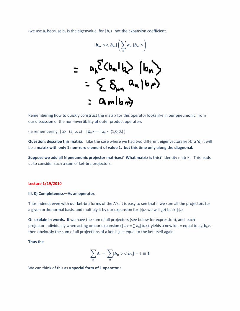
(we use an because bn is the eigenvalue, for |bn>, not the expansion coefficient.    

| |  |  

 

Remembering how to quickly construct the matrix for this operator looks like in our pneumonic  from 

our discussion of the non‐invertibility of outer product operators 

(ie remembering  |α>   (a, b, c)    |ϕn> == |an>   (1,0,0,) ) 

Question: describe this matrix.   Like the case where we had two different eigenvectors ket‐bra ‘d, it will 

be a matrix with only 1 non‐zero element of value 1.  but this time only along the diagnonal. 

Suppose we add all N pneumonic projector matrices?  What matrix is this?  Identity matrix.   This leads 

us to consider such a sum of ket‐bra projectors. 

 

Lecture 1/19/2010 

III. K) Completeness—As an operator. 

Thus indeed, even with our ket‐bra forms of the Λ’s, it is easy to see that if we sum all the projectors for 

a given orthonormal basis, and multiply it by our expansion for |ψ> we will get back |ψ>   

Q:  explain in words.  If we have the sum of all projectors (see below for expression), and  each 

projector individually when acting on our expansion (|ψ> = ∑ an|bn>)  yields a new ket = equal to an|bn>, 

then obviously the sum of all projections of a ket is just equal to the ket itself again. 

Thus the 

    | |  

We can think of this as a special form of 1 operator :   

For our continuous kets, since by definition of continuous kets, the set of basis kets can be enumerated 

by numerical labels ξ that are “infinitesimally close to each other”.  Thus for continuous kets we need 

must express our completeness sum as an integral over all states… 

1 = ∫ dξ |ξ><ξ| 

This is a very important tool as it will allow us to prove and calculate many things using only the 

bra/kets  

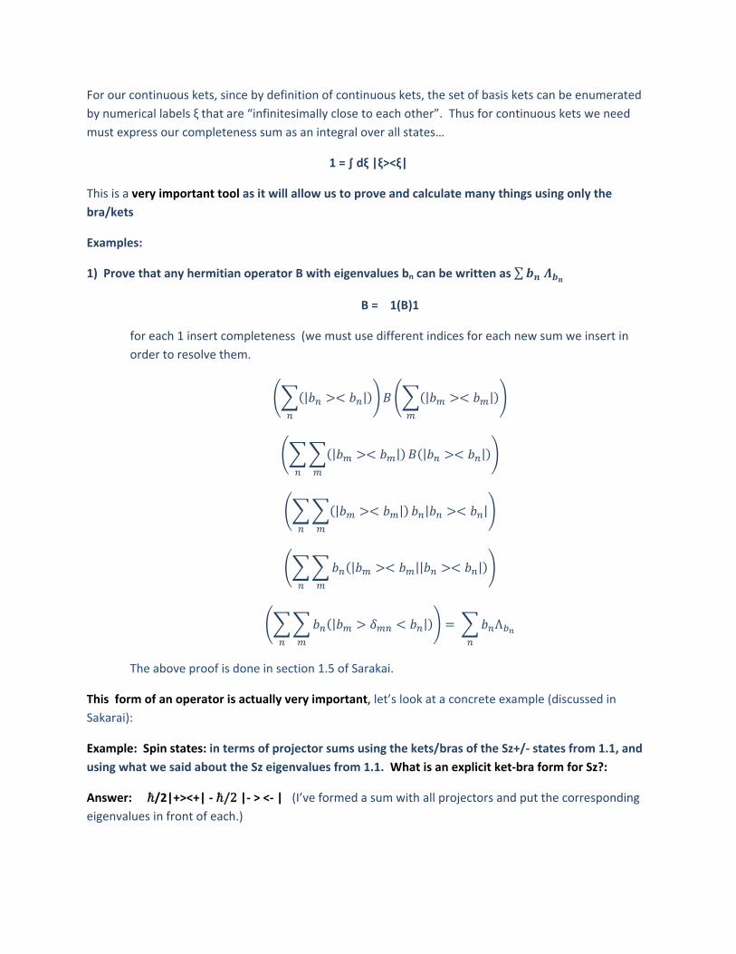
Examples: 

1)  Prove that any hermitian operator B with eigenvalues bn can be written as ∑    

B =    1(B)1 

for each 1 insert completeness  (we must use different indices for each new sum we insert in 

order to resolve them. 

| | | |  

| | | |  

| | | |  

| || |  

| |   Λ  

The above proof is done in section 1.5 of Sarakai. 

This  form of an operator is actually very important, let’s look at a concrete example (discussed in 

Sakarai):  

Example:  Spin states: in terms of projector sums using the kets/bras of the Sz+/‐ states from 1.1, and 

using what we said about the Sz eigenvalues from 1.1.  What is an explicit ket‐bra form for Sz?:   

Answer:      /2|+><+| ‐  /2 |‐ > <‐ |   (I’ve formed a sum with all projectors and put the corresponding 

eigenvalues in front of each.) 

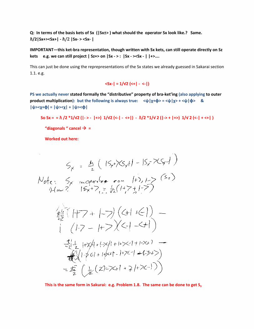
Q:  In terms of the basis kets of Sx  (|Sx±> ) what should the  operator Sx look like.?   Same.  

/2|Sx+><Sx+| ‐  /2 |Sx‐ > <Sx‐ |   

IMPORTANT—this ket‐bra representation, though written with Sx kets, can still operate directly on Sz 

kets     e.g. we can still project | Sz+> on |Sx ‐ > :  |Sx ‐ ><Sx ‐ | |+>….   

This can just be done using the reprepresentations of the Sx states we already guessed in Sakarai section 

1.1. e.g.  

<Sx‐| = 1/√2 (<+| ‐  <‐|) 

PS we actually never stated formally the “distributive” property of bra‐ket’ing (also applying to outer 

product multiplication):  but the following is always true:     <ψ|χ+ϕ> = <ψ|χ> + <ψ|ϕ>     &     

|ψ><χ+ϕ| = |ψ><χ| + |ψ><ϕ| 

So Sx =  =   /2 *1/√2 (|‐ > ‐  |+>)  1/√2 (<‐| ‐  <+|)  ‐   /2 *1/√ 2 (|‐> + |+>)  1/√ 2 (<‐| + <+| ) 

“diagonals “ cancel   =   

Worked out here:  

This is the same form in Sakurai:  e.g. Problem 1.8.  The same can be done to get Sy 

   

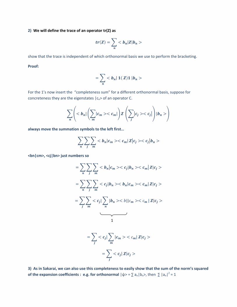
2)  We will define the trace of an operator tr(Z) as 

| | 

 

show that the trace is independent of which orthonormal basis we use to perform the bracketing. 

Proof:   

|     | 

 

For the 1’s now insert the  “completeness sum” for a different orthonormal basis, suppose for 

concreteness they are the eigenstates |cn> of an operator C. 

| | | 

  

| 

  

always move the summation symbols to the left first… 

| |   

 

<bn|cm>, <cj|bn> just numbers so 

| 

|  

 

| | | 

|  

 

| | 

|| 

|  | 

 

 

 

| | 

|  | 

 

|  | 

 

3)  As in Sakarai, we can also use this completeness to easily show that the sum of the norm’s squared 

of the expansion coefficients :  e.g. for orthonormal |ψ> = ∑ an|bn>, then  ∑ |an|2 = 1   

1

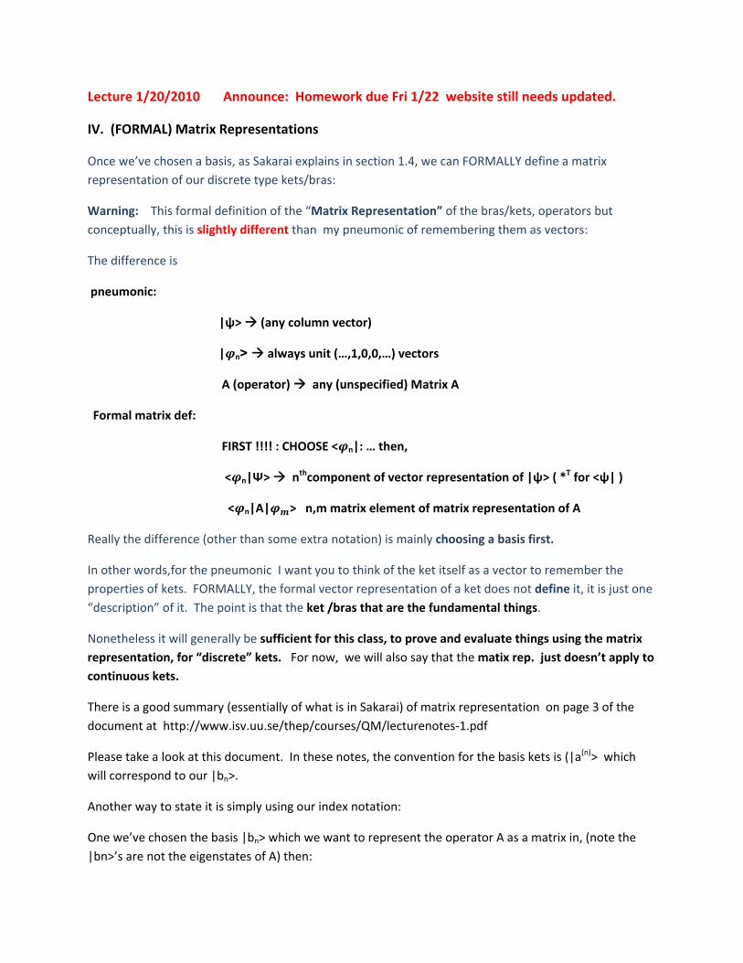
Lecture 1/20/2010       Announce:  Homework due Fri 1/22  website still needs updated. 

IV.  (FORMAL) Matrix Representations   

Once we’ve chosen a basis, as Sakarai explains in section 1.4, we can FORMALLY define a matrix 

representation of our discrete type kets/bras: 

Warning:    This formal definition of the “Matrix Representation” of the bras/kets, operators but 

conceptually, this is slightly different than  my pneumonic of remembering them as vectors:   

The difference is 

 pneumonic:     

|ψ>  (any column vector)   

| n>  always unit (…,1,0,0,…) vectors    

 A (operator)   any (unspecified) Matrix A  

Formal matrix def: 

 FIRST !!!! : CHOOSE < n|: … then,  

  < n|Ψ>   nthcomponent of vector representation of |ψ> ( *T for <ψ| )  

   < n|A| >   n,m matrix element of matrix representation of A  

Really the difference (other than some extra notation) is mainly choosing a basis first.  

In other words,for the pneumonic  I want you to think of the ket itself as a vector to remember the 

properties of kets.  FORMALLY, the formal vector representation of a ket does not define it, it is just one 

“description” of it.  The point is that the ket /bras that are the fundamental things. 

Nonetheless it will generally be sufficient for this class, to prove and evaluate things using the matrix 

representation, for “discrete” kets.   For now,  we will also say that the matix rep.  just doesn’t apply to 

continuous kets.   

There is a good summary (essentially of what is in Sakarai) of matrix representation  on page 3 of the 

document at  http://www.isv.uu.se/thep/courses/QM/lecturenotes‐1.pdf 

Please take a look at this document.  In these notes, the convention for the basis kets is (|a(n)>  which 

will correspond to our |bn>.   

Another way to state it is simply using our index notation: 

One we’ve chosen the basis |bn> which we want to represent the operator A as a matrix in, (note the 

|bn>’s are not the eigenstates of A) then:  

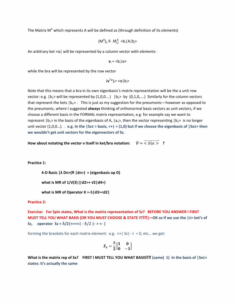
The Matrix MA which represents A will be defined as (through definition of its elements) 

(MA)ij ≡     <bi|A|bj> 

An arbitrary ket <α| will be represented by a column vector with elements:  

vi = <bi|α> 

while the bra will be represented by the row vector 

(vT*)i= <α|bi>  

Note that this means that a bra in its own eigenbasis’s matrix representation will be the a unit row 

vector: e.g. |b1> will be represented by (1,0,0….)   |b2>  by  (0,1,0,….)  Similarly for the column vectors 

that represent the kets |bn> .   This is just as my suggestion for the pneumonic—however as opposed to 

the pneumonic, where I suggested always thinking of orthonormal basis vectors as unit vectors, if we 

choose a different basis in the FORMAL matrix representation, e.g. for example say we want to 

represent |b1> in the basis of the eigenbasis of A, |an>, then the vector representing |b1>  is no longer 

unit vector (1,0,0…).  .  e.g. In the |Sz± > basis, <+| = (1,0) but if we choose the eigenbasis of |Sx±> then 

we wouldn’t get unit vectors for the eigenvectors of Sz. 

How about notating the vector v itself in ket/bra notation:         |     ? 

 

Practice 1:  

  4‐D Basis |λ Dn>(≡ |dn>)  = (eigenbasis op D)       

what is MR of 1/√(3) (|d2>+ √2|d4>) 

what is MR of Operator K =‐5|d3><d2| 

Practice 2:  

Exercise:   For Spin states, What is the matrix representation of Sz?   BEFORE YOU ANSWER I FIRST 

MUST TELL YOU WHAT BASIS (OR YOU MUST CHOOSE & STATE IT‼‼)—OK so if we use the |±> ket’s of 

Sz,     operator  Sz =  /2|+><+| ‐  /2 |‐ > <‐ | 

forming the brackets for each matrix element:  e.g.  <+| Sz|‐ >  = 0, etc… we get: 

 

What is the matrix rep of Sx?    FIRST I MUST TELL YOU WHAT BASIS‼‼ (same)  1)  In the basis of |Sx±> 

states: it’s actually the same  

 

IN THE BASIS of the Sz states.   We can actually do it.  But first we should construct the Sx operator in ket 

and bras.   BUT WE ALREADY HAVE IT‼‼ 

We already said Sx     /2|Sx+><Sx+| ‐  /2 |Sx‐ > <Sx‐ |  and we already said it this can act on +/‐kets /bras  including eigenstates of any  Operator, including Sz.   

In this sense the ket‐bra representations are “independent” of what basis you decide to work in. 

Thus to get the matrix representation,in the basis of the Sz states we need to know how evaluate inner 

products like <Sx‐|+>.     

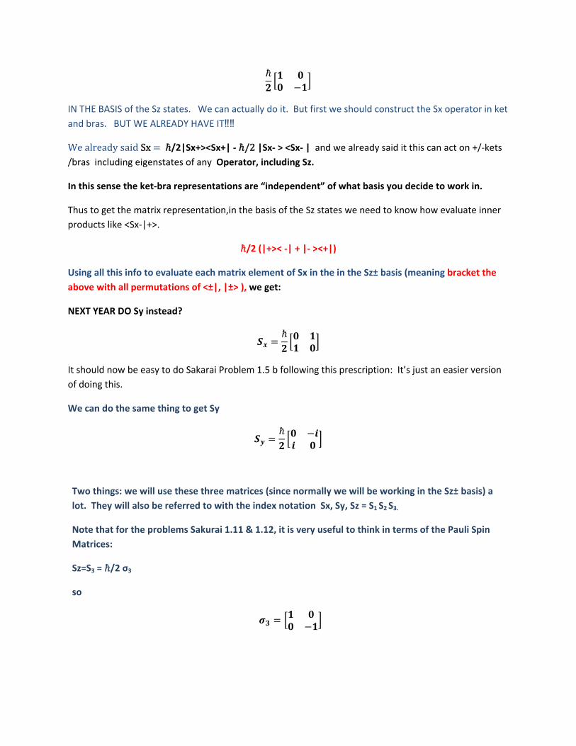
/2 (|+>< ‐| + |‐ ><+|) 

Using all this info to evaluate each matrix element of Sx in the in the Sz± basis (meaning bracket the 

above with all permutations of <±|, |±> ), we get: 

NEXT YEAR DO Sy instead? 

 

It should now be easy to do Sakarai Problem 1.5 b following this prescription:  It’s just an easier version 

of doing this.    

We can do the same thing to get Sy 

 

 

Two things: we will use these three matrices (since normally we will be working in the Sz± basis) a 

lot.  They will also be referred to with the index notation  Sx, Sy, Sz = S1 S2 S3. 

Note that for the problems Sakurai 1.11 & 1.12, it is very useful to think in terms of the Pauli Spin 

Matrices: 

Sz=S3 =  /2 σ3   

so  

 

etc…   there are a lot of useful properties of these matrices listed on page 165 of Sakarai.   e.g.  {σi,σ j} = 

2 δ ij (some of which are repeated in this chapter in terms of the S matrices.) It will definitely be useful 

for the problem set to use some of these properties. 

 

Equally or probably more important as the matrix rep of operators (which are actual matrices, hence the 

name “matrix rep”) is the matrix representation of the state kets.  These will be the vectors  with n 

components < n|Ψ>   We should always represent the kets in the matrix representation using the 

same basis kets we use to rep the operators, so following the above examples,we will want to 

represent an arbitrary state |α > in the |±> basis.  The matrix rep vector of |α> will have 2 

components <+|α> and <‐|α>: 

||      

As a concrete example we could think of the state |α> = |Sx‐> : . 

Matrix Rep( |S‐> )  /√/√

 

 

Digression:   Help on Problem 1.11) Sakurai 

Here is the road map of doing this problem using the hint: 

1) Write the matrix representation of H in the |1>,|2> orthonormal basis –this will be a 2x2 matrix 

whose elements are the constants in front of the outer products:, e.g. H11 

2a) From here you could just approach the problem like the quiz problem of finding eigenvalues/vectors 

in Linear Algebra.  The vector   you get obviously represents a|1>+b|2>.  Messy: λ ‘s will be some fn’s 

of H11, H12, etc…  but DONE… you need not follow the next steps… 

2b) BUT INSTEAD to use the hint though, then the exact same way you did last week in problem 1.2,  

write that  2x2 matrix H in the 1.2  form.    

The answer looks like this:        +  ΔH σ3 + H12σ1   (for a clever but not so hard to think of choice 

of  , Δ  ) 

Thus the   of 1.2 in this case is the vector (H12,0,Δ H)    

3) The connection to hint about the eigenvector  of S· n  is that S· n    σ · a .   If H had only the σ· a term,  you obviously could just use the given hint answer with the substitution  |   |1  and |‐   |2  and for γ β  such that      

4  But from Linear Algebra:  Eigenvectors of matrix A are same as Eigenvectors of matrix  A xI  try it! .  So 1.2 form should still have given hint  eigenvector form, so then find γ, β from step 3 in terms of constants H11 etc… 

cos 2β  = Δ H2/(Δ H2 + H122)2 

For  1.12:  use 1.11 results:    γ → β 

Lecture 1/22/2010  ‐‐‐ Homework next week will again be due on Fri:  let me know about other 

class’s midterms—we need to schedule ours.     

V.  Measurement  (Part 1) 

A) Postulates 

Three Postulates concerning Measurements in Quantum Mechanics: 

Postulate 1)  The only possible values for a measurement of an observable B, will be the possible 

eigenvalues of the Hermitian operator representing B.   (How to find the operator B if don’t already 

know the eigenvalues we want e.g. through first measuring them! == empirically determining them, will 

be discussed later, and is not specified by this postulate). 

Postulate 2)    Before measurement for a quantum system in the state |α>, the probability to measure 

eigenvalue bn of B will be given by |<bn|α>|2  which defines the probability distribution P(n) for each 

state n.   During measurement an eigenvalue bn will be randomly chosen, according to the probability 

distribution  P(n).      1   2 | |   | | |  

Postulate 3)   Immediately after measurement, the system will “collapse”  into a new state that is 

completely in the direction of the eigenstate |bn>  or in some cases, when there is something called 

degeneracy,  to an “eigen” sub‐space defined below, corresponding to the chosen bn. 

Notice the postulates are not specific about how to mathematically represent this measurement  

Can measurement be represented by operating with the projection operator?   The plain projection 

operator acting on a state, will give back a state that is no longer properly normalized.    Thus we 

could think of this as a way to mathematically represent measurement, but we would have to specify 

that the state afterwards benormalized again.   

This is easy to see by thinking of Successive measurements…   Successive projection operators might 

keep reducing the normalization of the state.   One might be tempted to equate this with our Stern‐

Gerlach experiment, where each time we “block a state” we are removing half of our Ag beam, and thus 

successively reducing the intensity of the beam.   It is important to realize this is NOT EXACTLY THE 

CASE.  Because if we only consider what is happening to 1 Ag atom alone,  after it “survives” one filter, it 

still has probability of 1 to go either way in the next filter.  (In thinking about the beam intensity/”flux” 

of Ag, as a whole though this may not be a such a bad model.) 

Thinking about whether it doesn’t survive the filter, This is related to another point that contains the 

essence of Quantum Mechanics:  without the S‐G  there, in fact, no definite state is chosen.    One 

must be careful. 

B)   Expectation Values   

If we know the probability of all outcomes, we can calculate what the outcome will be on average: 

  Average weighted by the probabilities:   

    

Sum C P(C)   This is the most important relations to apply to science.  Use it all the time in 

experimental physics… 

Since by our postulates above P(bn) =|<bn|α>|2 , for any general state α  then  it is easy to see, thinking 

of our projector form of the operator B, that this expectation value can also be written 

<α|B|α> 

This we already know from wave mechanics.  We will discuss how the wave mechanics version of the 

expectation value fits in to our new formalism this week. 

C) Compatatible/incompatible observables. 

If [A,B] == 0, then A and B, along with their observables,  are called compatible 

Else they are called incompatible. 

Good examples are angular momentum matrices.  (we will demonstrate with our Pauli matrices σi)  

From wave mechanics, L2 and Lz are compatible, while Lz, Lx are incompatible.   Similarly for our spin 

matrices we can define the operator S2 

S2     SxSx SySy SzSz    2/4 σ12   σ22 σ32  

Here are some useful properties of the σ matrices, you can check w/ the matrices themselves: 

σ i σ j = iϵ ijk σ k +   δ ij 

e.g. (σ 1 σ 2 sheet)  ‐‐try it with the matrices themselves e.g.   σx 2 

which also implies 

{σi,σ j} = 2 δ ij 

[σi,σ j] = iϵ ijk σ k 

One thing that is interesting from these relations is that  

S2 =  2/4            3  2/4 

There fore it is obvious that S2 commutes with every operator.   This includes the Si..   It is compatible 

with any of them.   On the other hand each Si is incompatible with any of the others. 

Starting 1.11/1.12.  While we’re on the subject of the σ matrices and their properties, let’s talk about 

a few hints for the problems 1.11:   

  

D)  Non‐commuting (Incompatible) Operators cannot have common eigenstates.   

Suppose |ϕ n > were an eigenvalue of both A and B.    Then 

[A,B]|ϕ n> = anbn|ϕ n> ‐bnan|ϕ n> = 0.     But by first definitions of operators this implies [A,B] = 0.  

 

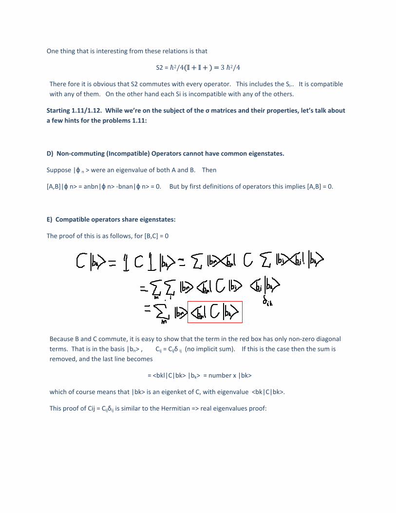
E)  Compatible operators share eigenstates:    

The proof of this is as follows, for [B,C] = 0 

 

Because B and C commute, it is easy to show that the term in the red box has only non‐zero diagonal 

terms.  That is in the basis |bn> ,        Cij = Cijδ ij  (no implicit sum).    If this is the case then the sum is 

removed, and the last line becomes   

= <bkl|C|bk> |bk>  = number x |bk> 

which of course means that |bk> is an eigenket of C, with eigenvalue  <bk|C|bk>. 

This proof of Cij = Cijδij is similar to the Hermitian => real eigenvalues proof: 

 

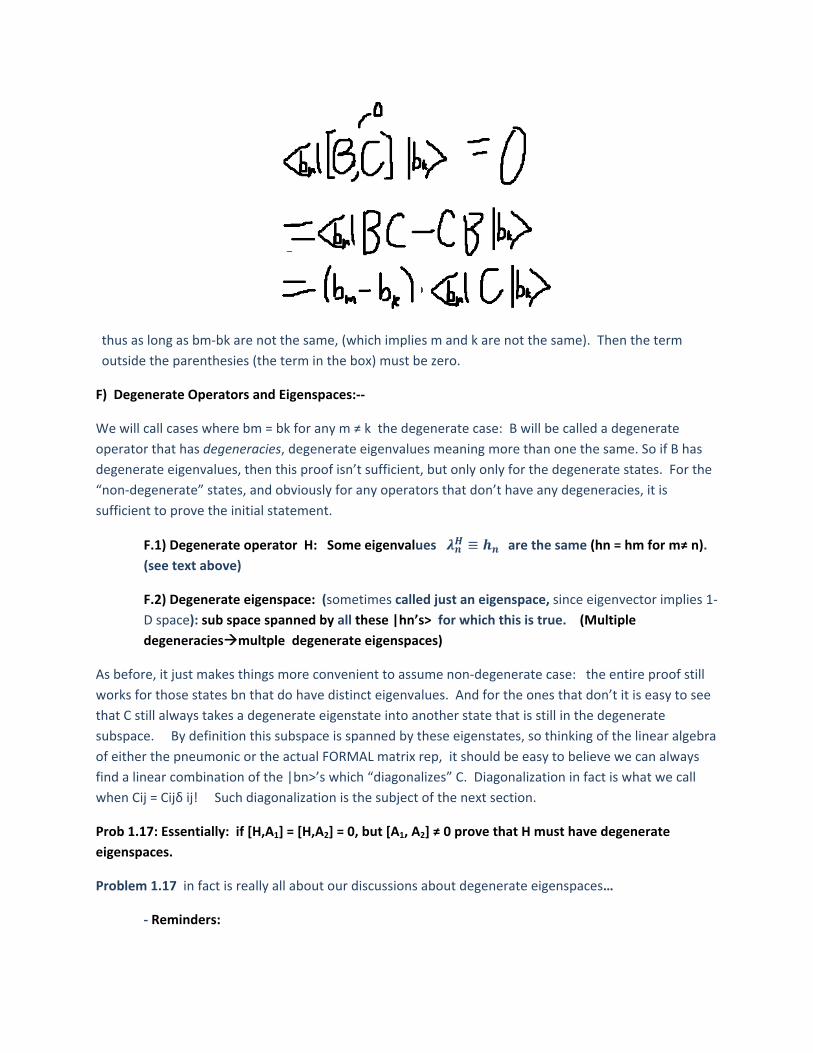
thus as long as bm‐bk are not the same, (which implies m and k are not the same).  Then the term 

outside the parenthesies (the term in the box) must be zero.    

F)  Degenerate Operators and Eigenspaces:‐‐ 

We will call cases where bm = bk for any m ≠ k  the degenerate case:  B will be called a degenerate 

operator that has degeneracies, degenerate eigenvalues meaning more than one the same. So if B has 

degenerate eigenvalues, then this proof isn’t sufficient, but only only for the degenerate states.  For the 

“non‐degenerate” states, and obviously for any operators that don’t have any degeneracies, it is 

sufficient to prove the initial statement. 

F.1) Degenerate operator  H:   Some eigenvalues       are the same (hn = hm for m≠ n).   

(see text above)  

F.2) Degenerate eigenspace:  (sometimes called just an eigenspace, since eigenvector implies 1‐

D space): sub space spanned by all these |hn’s>  for which this is true.    (Multiple 

degeneraciesmultple  degenerate eigenspaces) 

As before, it just makes things more convenient to assume non‐degenerate case:   the entire proof still 

works for those states bn that do have distinct eigenvalues.  And for the ones that don’t it is easy to see 

that C still always takes a degenerate eigenstate into another state that is still in the degenerate 

subspace.     By definition this subspace is spanned by these eigenstates, so thinking of the linear algebra  

of either the pneumonic or the actual FORMAL matrix rep,  it should be easy to believe we can always 

find a linear combination of the |bn>’s which “diagonalizes” C.  Diagonalization in fact is what we call 

when Cij = Cijδ ij!     Such diagonalization is the subject of the next section. 

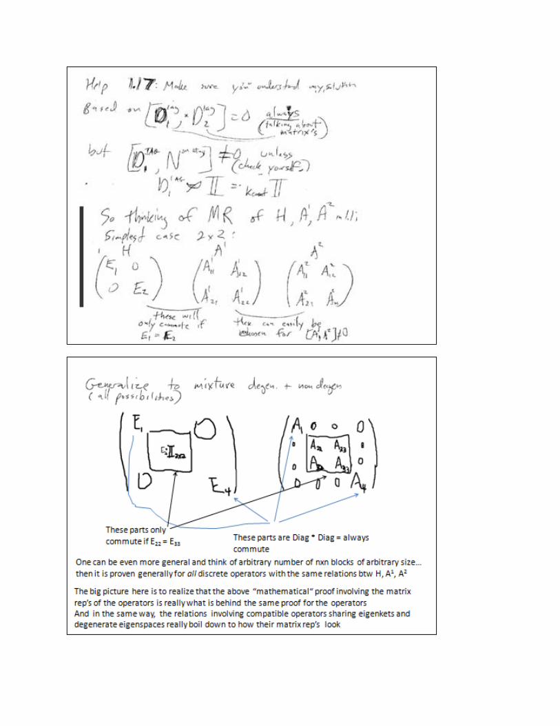
Prob 1.17: Essentially:  if [H,A1] = [H,A2] = 0, but [A1, A2] ≠ 0 prove that H must have degenerate 

eigenspaces. 

Problem 1.17  in fact is really all about our discussions about degenerate eigenspaces… 

‐ Reminders: 

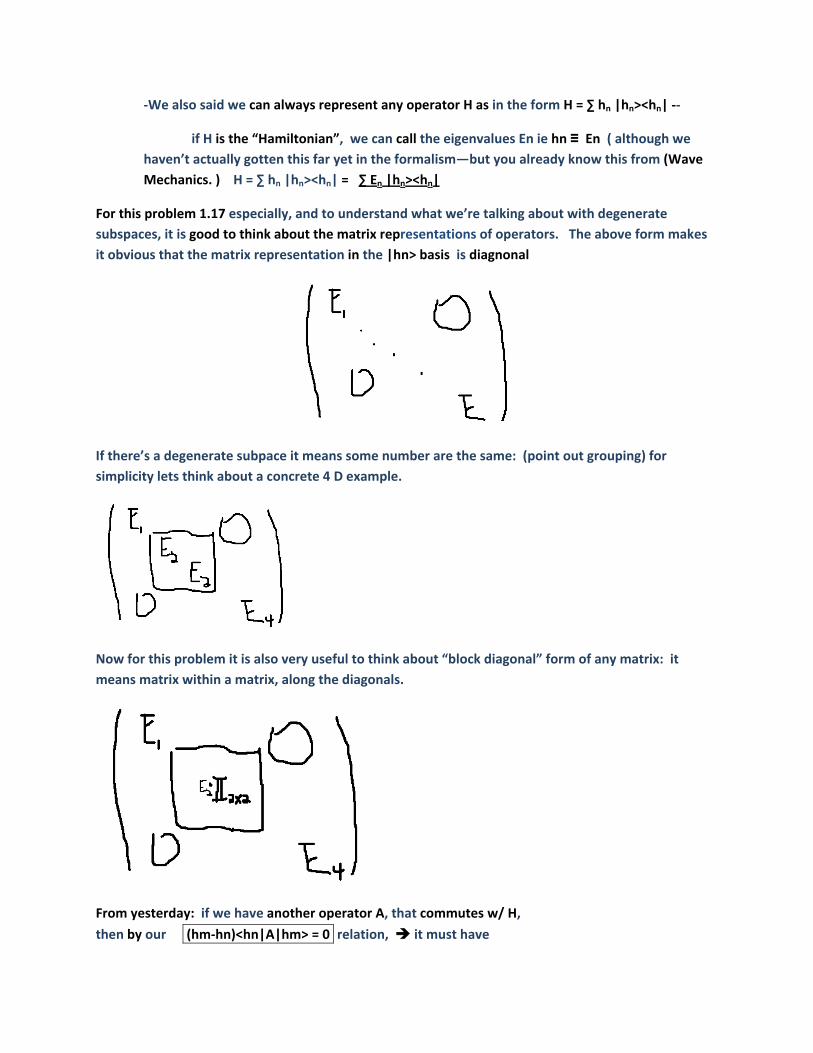
   ‐We also said we can always represent any operator H as in the form H = ∑ hn |hn><hn| ‐‐  

if H is the “Hamiltonian”,  we can call the eigenvalues En ie hn ≡  En  ( although we 

haven’t actually gotten this far yet in the formalism—but you already know this from (Wave 

Mechanics. )    H = ∑ hn |hn><hn| =   ∑ En |hn><hn| 

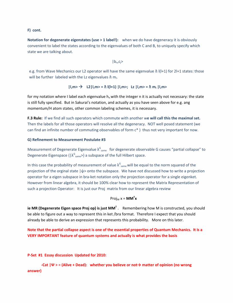
For this problem 1.17 especially, and to understand what we’re talking about with degenerate 

subspaces, it is good to think about the matrix representations of operators.   The above form makes 

it obvious that the matrix representation in the |hn> basis  is diagnonal 

 

If there’s a degenerate subpace it means some number are the same:  (point out grouping) for 

simplicity lets think about a concrete 4 D example. 

 

Now for this problem it is also very useful to think about “block diagonal” form of any matrix:  it 

means matrix within a matrix, along the diagonals. 

 

From yesterday:  if we have another operator A, that commutes w/ H,               

then by our      (hm‐hn)<hn|A|hm> = 0  relation,   it must have  

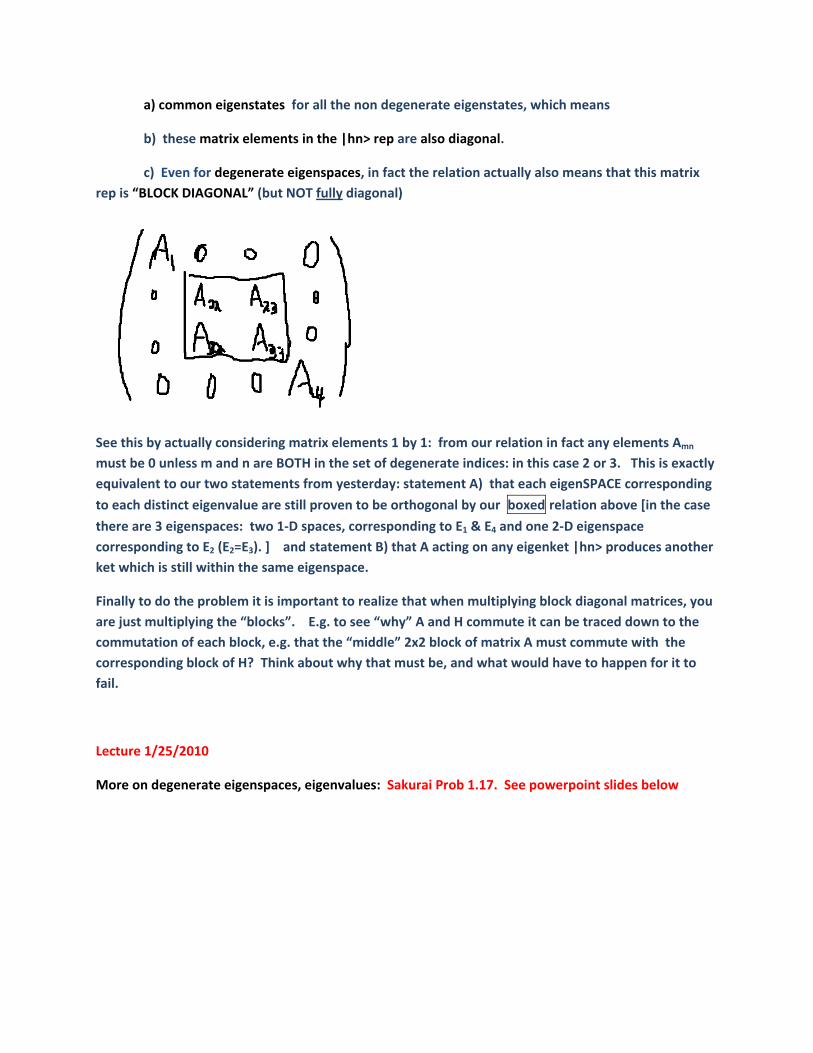
a) common eigenstates  for all the non degenerate eigenstates, which means   

b)  these matrix elements in the |hn> rep are also diagonal.   

c)  Even for degenerate eigenspaces, in fact the relation actually also means that this matrix 

rep is “BLOCK DIAGONAL” (but NOT fully diagonal) 

 

See this by actually considering matrix elements 1 by 1:  from our relation in fact any elements Amn 

must be 0 unless m and n are BOTH in the set of degenerate indices: in this case 2 or 3.   This is exactly 

equivalent to our two statements from yesterday: statement A)  that each eigenSPACE corresponding 

to each distinct eigenvalue are still proven to be orthogonal by our  boxed relation above [in the case 

there are 3 eigenspaces:  two 1‐D spaces, corresponding to E1 & E4 and one 2‐D eigenspace 

corresponding to E2 (E2=E3). ]    and statement B) that A acting on any eigenket |hn> produces another 

ket which is still within the same eigenspace.      

Finally to do the problem it is important to realize that when multiplying block diagonal matrices, you 

are just multiplying the “blocks”.    E.g. to see “why” A and H commute it can be traced down to the 

commutation of each block, e.g. that the “middle” 2x2 block of matrix A must commute with  the 

corresponding block of H?  Think about why that must be, and what would have to happen for it to 

fail. 

 

Lecture 1/25/2010   

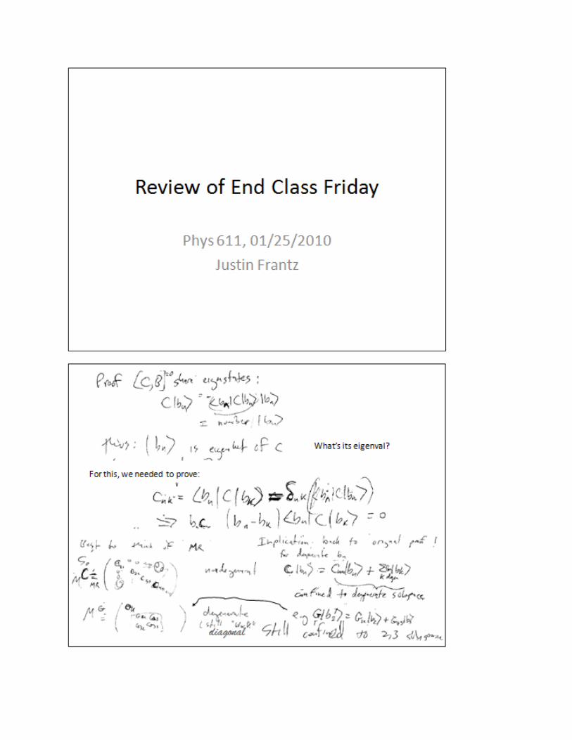
More on degenerate eigenspaces, eigenvalues:  Sakurai Prob 1.17.  See powerpoint slides below 

 

 

 

 

 

F)  cont.   

Notation for degenerate eigenstates (use > 1 label!):    when we do have degeneracy it is obviously 

convenient to label the states according to the eigenvalues of both C and B, to uniquely specify which 

state we are talking about. 

|bn,cj> 

e.g. from Wave Mechanics our L2 operator will have the same eigenvalue   l(l+1) for 2l+1 states: those 

will be further  labeled with the Lz eigenvalues   ml.      

|l,m>     L2|l,m> =   l(l+1) |l,m>;   Lz |l,m> =   ml |l,m> 

for my notation where I label each eigenvalue hn with the integer n it is actually not necessary: the state 

is still fully specified.  But in Sakurai’s notation, and actually as you have seen above for e.g. ang 

momentum/H atom states, other common labeling schemes, it is necessary. 

F.3 Rule:  If we find all such operators which commute with another we will call this the maximal set.  

Then the labels for all those operators will resolve all the degeneracy.  NOT well posed statement (we 

can find an infinite number of commuting observables of form c* )  thus not very important for now. 

G) Refinement to Measurement Postulate #3  

Measurement of Degenerate Eigenvalue λGsame   for degenerate observable G causes “partial collapse” to 

Degenerate Eigenspace {|λGsame>} a subspace of the full Hilbert space. 

In this case the probability of measurement of value λGsame will be equal to the norm squared of the 

projection of the orginal state |ψ> onto the subspace.  We have not discussed how to write a projection 

operator for a eigen subspace in bra‐ket notation only the projection operator for a single eigenket.  

However from linear algebra, it should be 100% clear how to represent the Matrix Representation of 

such a projection Operator:   It is just our Proj  matrix from our linear algebra review 

ProjW x = MMTx 

ie MR (Degenerate Eigen space Proj op) is just MMT .    Remembering how M is constructed, you should 

be able to figure out a way to represent this in ket /bra format.  Therefore I expect that you should 

already be able to derive an expression that represents this probability.   More on this later.   

Note that the partial collapse aspect is one of the essential properties of Quantum Mechanics.  It is a 

VERY IMPORTANT feature of quantum systems and actually is what provides the basis  

 

P‐Set  #1  Essay discussion  Updated for 2010:   

‐Cat |Ψ > = (Alive + Dead):   whether you believe or not→ matter of opinion (no wrong 

answer) 

  ‐however, I don’t believe, I think most physicists are skeptical at best…(this is something 

philosophers like to debate, not physicists as much.)   Think of this:  why isn’t the cat a valid 

observer—observation depends on IQ?    Roger Penrose (famous mathematician) has theory of 

thought having quantum roots which is supposed to explain this, so my guess is there must be some 

way to validly pose the “thought == measurement” theory.   Thus I will not discount it completely. 

However for this class, we will never rely on this argument. 

  But the reasons for me not believing Cat = Alive + Dead have to do with details of the cat 

being a large complex system, and I don’t believe the quantum mechanics of simple states like in the 

SG expereiment apply to it as a whole without some further specifications.   That is I don’t believe one 

can so simply connect the cat to the simpler 2‐state system.  I do believe that the 2‐state system is in 

the “Alive + Dead” superposition, and in that sense the Alive + Dead way of thinking is the more 

correct quantum mechanical intuition. 

‐‐‐‐‐‐‐‐‐‐‐‐‐‐‐‐‐‐‐‐‐‐‐‐‐‐‐‐‐‐‐‐‐‐‐‐‐‐‐‐‐‐‐‐‐‐‐‐‐‐‐‐‐‐ 

Screen or  B field… (I will accept all answers as long as they were justified)  

    ‐FIRST almost no one said “after”—(eyes see?)—this would be equivalent to 

thought==measurement :  

‐Good!   Important point:  not just a question of “does the falling tree make noise if no 

one hears it”?   We don’t want to answer that question in this class.   We are only concerned 

w/ things we can test in science—by definition that is an untestable question. 

‐I’m not 100% sure of answer myself:  For this course,  we are only concerned with 

BOTH Mag + Filter/Screen.  So as Sakurai never does, I will not be able to give you a definite 

answer for now—we will discuss the situation a little further though, and after that we will be 

able to say more.  Also we will see in the next section how we can find out for sure by expt—

which is really the most important determiner.    

‐The safest answer is the screen.  True, the B field by itself should do SOMETHING.    

But even for the single atom, if there is no screen,  the  two possible states |±> should have an 

Quantum Mechanical interference effect, much like when a single electron beam goes through a 

double slit collimator and exhibits an interference pattern that is equivalent to a superposition 

of it going through both slits.   So as with the electron, it may depend on actual wave function 

considerations of the changes in trajectory (meaning the space wave function from wave 

mechanics, which of course still is part of the atom’s quantum description—for example, will the 

beam split be small or large‐‐something that is ignored in this thought experiment) as to 

whether such an interference will occur, and thus whether a full collapse has occurred in the 

magnetic field alone occurring in the SG at the B field or screen 

So taking the interference effect into account, my best answer is that the B‐field by 

itself (without the screen)  is a “partial” measurement that causes a partial collapse:  the state 

is collapsed into a superposition of +/‐ for whatever the direction of the Bfield was, but it does 

not necessarily choose one or the other:  it can in fact be left in a state that is the 

superposition of both.     

Part of this question has to do with whether initial state are a “pure state” or a “mixed 

state” something we will discuss later in the course. 

 

H)  Consequence of Measurements (Summary) 

For Degenerate Observables:  For an observable that has a corresponding operator which is degenerate, 

measurement of (only) that observable which results in the degenerate eigenvalue being measured  will 

only cause a “partial collapse” of the state into the degenerate subspace.   The exact state within the 

subspace is not generally affected by the measurement, and is still uncertain. 

For compatible observables: During two successive measurements of two different but compatible 

observables, the second  measurement can not change the state in such a way that the previously 

measured eigenvalue, if measured again, will not be measured again.   

“Measurements of Compatible Observables do not interfere” 

 Incompatible Observables:  on the other hand: During two successive measurements of in compatible 

observables, the second measurement causes a “re‐collapse” of the state which changes the probability 

of subsequent measurements. 

“Measurements of Incompatible Observables DO interfere” 

 

I)  Example of Measurement Interference   

Consider the following set of S‐G –like apparatuses applied in succession:  3 observables A, B, C, and a 

filter for only picking one of the eigenstates. 

 

If before going through measurement filter A, our quantum state (think of the state of an atom flying 

through all three, like in SG)  is some arbitrary state |α> , then we can write the total probability to have 

the set of measurements indicated in the drawing (an, bn, cn) as Ptot = |<α|a>|2 Pa→b→c where Pa→b→c is 

Pabc = |<cn|bn>|2|<bn|an>|2 ( 

Could’ve labeled it ak, cj, bnmeans the same—thus let’s just use a, b,c .  We can rewrite Pabc  as <c|b><b|a><a|b><b|c>   Thus, the sum over all measured b routes to get one particular a→c  combination , Pa→c

b   as     

Pa→cb = ∑b  <c|b><b|a><a|b><b|c> 

Notice there is only one sum over all the b states.   

Now compare to  if we remove b completely from the picture  

 

(we can just imagine the presence of B) 

For here Pa→c is just |<c|a>|2 which can be rewritten inserting 2 closure sums over b (the concrete 

expression of our b imagination), and therefore two different sums over b 

Pa→c = ∑ n∑ m <c|bn><bn|a><a|bm><bm|c> 

Notice:  it is not the same as Pa→cb  N‼‼ 

Neat.  Huh good demonstration of the essence of the weirdness that is at the heart of Quantum Mech. 

But really this is not very hard to understand what’s going on here or really very “surprising”  what we 

already stated about measurements in general.   

Why it’s not hard to understand:  Thinking of routes “through b states” is very helpful to understanding 

this:    

Q explain in terms of what b states are “gone through” in each case:  what routes? every time 

it’s going through all states of |b> at once. N routes.   As opposed to going 1 route N times.   

Think of a traffic:  it only 1 road is open out of N.  the resulting traffic will certainly not flow as 

efficiently. 

Why it’s not too surprising: it is just a result of the collapse of that occurs from the measurement of b).   

All it is saying is that |a> = ∑ c|b> ≠ |b>   

How to use this result to answer our question of where the collapse in the Stern‐Gerlach takes place 

definitively – in the B field or when it hits the screen/filter? 

Actually it’s not this relation per se that could prove it for us, but using 3 successive SG we could at least 

gain some valuable insight:   Suppose we repeat our first “MORE INTERESTING” SG experiment w/ 3 

successive SG’s 

SG1: z field filter  SG2:  x field filter SG3:  z field filter 

Now just remove the filter part of SG2 leaving only the x B field.  Our argument before was that we were 

“removing half of zero” w/ the x filter, which caused a new state with both Sz components again.  So if 

the magnetic field caused z field to again have both components then it is likely that the x field alone did 

cause a collapse.   Though it is still not clear whether the collapse was in the x+ or x‐ direction.  

Note that in class I did think we could also determine whether or not the collapse was occurring by 

comparing probability sums just like the above case w/ A, B, C.  Although seemingly in need of the actual 

filter I believe there may be a way around not having an actual filter, by averaging over all possible filter 

configurations, and comparing that sum to going without the filter, but only having the field.    I still 

think this may be possible using a single atom beam (ie one Ag atom at a time), but I do not have time to 

figure it out—if you’ve thought of a way, please let me know… 

   

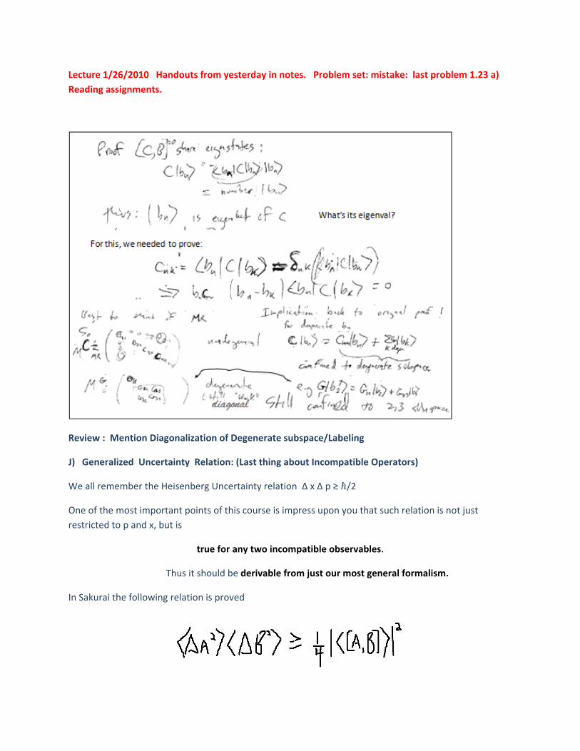
Lecture 1/26/2010   Handouts from yesterday in notes.   Problem set: mistake:  last problem 1.23 a)  

Reading assignments. 

 

 

Review :  Mention Diagonalization of Degenerate subspace/Labeling 

J)   Generalized  Uncertainty  Relation: (Last thing about Incompatible Operators) 

We all remember the Heisenberg Uncertainty relation  Δ x Δ p ≥  /2 

One of the most important points of this course is impress upon you that such relation is not just 

restricted to p and x, but is  

true for any two incompatible observables. 

Thus it should be derivable from just our most general formalism. 

In Sakurai the following relation is proved 

 

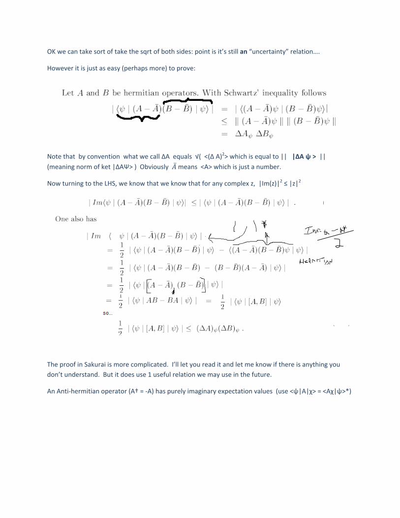
OK we can take sort of take the sqrt of both sides: point is it’s still an “uncertainty” relation…. 

However it is just as easy (perhaps more) to prove: 

 

Note that  by convention  what we call ΔA  equals  √(  <(Δ A)2> which is equal to ||   |ΔA ψ >  || 

(meaning norm of ket |ΔAΨ> )  Obviously    means  <A> which is just a number.    

Now turning to the LHS, we know that we know that for any complex z,  |Im(z)|2 ≤ |z|2 

 

 

The proof in Sakurai is more complicated.  I’ll let you read it and let me know if there is anything you 

don’t understand.  But it does use 1 useful relation we may use in the future. 

An Anti‐hermitian operator (A† = ‐A) has purely imaginary expectation values  (use <ψ|A|χ> = <Aχ|ψ>*)  

 

   

Lecture 1/27/2010 Note:  scanned version of chalkboard notes (more condensed version of text) at 

end 

VI) Transformation Operators  

A) Introduction 

We had mentioned diagonalization: in our discussion of degenerate spaces:  the idea was we said there 

is we could always find a set of basis vectors |ϕn> for which the following would be true for A   

diagonalization:   <ϕm|A|ϕn>  =   <ϕn|A|ϕm> δmn   (no implied sum) 

This is just a completely literal statement of the fact that the matrix representation of A in this basis is 

diagonal  

Remembering from linear algebra that the way we diagonalize matrices means that we  

find  the matrix S such that we can form the matrix    D = S‐1AS   where S‐1S = 1. 

We also remember if it’s a symmetric matrix (if AT = A) then S‐1 = ST.    

For operators we will think of the matrix S  operator U called the “transformation operator”. 

Just as for symmetric matrices, for hermitian operator B (B=B†), the operator UB = U which diagonalizes 

it, will always have the property that U† = U‐1 or  

UU†=U† U =   

 Note that such an operator is NOT hermitian in general (but could be in specific cases? e.g. Proj 

operators?).   

We will remember for matrices, that this is essentially equivalent to finding the eigenvectors of the 

matrix, since S is made up of the eigenvectors.   (ev1|ev2|…)  On the operator side, if we have a 

mathematical form for the operator, and we have a complete set of basis states, it is the problem of 

finding the expansion of each eigenstate in the old basis: 

|bn> =∑  cm |am>   

that is, finding the coefficients cm  for every n ([cm]n) : this will be the ingredients for forming U (in fact 

we will find, Umn (matrix rep)  = [cm]n.)   Note however simply expanding |an> in the |b> basis is not 

what is performed when we apply U to a ket: ie it’s not what we use U for.  For that all we need is to 

insert closure = 1 → |b> = ∑ |a><a|b>.    What we DO with U is very different  as we shall see.  

 You might be thinking at this point: don’t we already have the answer for what U is:    [cm]n = <am|bn>?  

The answer is actually true –however you’ve missed the point:  to calculate <am|bn>, we need first 

need the expansion parameters [cm]n !   So then we can actually calculate <am|bn>  =  as 

<am|( ∑  ck |ak> 

 –only in this form do we know how to “remove” the innerproducts.  

B) Tempting Confusions in Sakurai:   

1) Above:  Bra/ket expressions so simple (e.g. Bra/ket form given for U)  one thinks there is 

magic ket way of avoiding Linear Algebra work w/ Matrices to find eigenvectors.   There isn’t, you must 

still do the same Linear Algebra operations   

2)  simple expansion in different bases (passive rotations) which is performed with the 

completeness operator (ie 1)  with b) the action of U (which is to actively rotate vectors).  

 

C) Action:  What does this transformation operator actually DO?: 

Let’s think deeper about this.   We said ALL operators are transformations.  How are these 

“transformation transformations”  different? 

When we diagonalize a matrix what are we actually doing?  Answer: we have a set of basis vectors   , 

that are unit vectors .e.g  0,1,0…   and we have some matrix B which has eigenvectors  n which 

are  NOT unit vectors, but when we diagonalize B, we “switch places” between the b’s and a’s:  now the 

b’s become the unit vectors, and the a’s will actually no longer be unit vectors in the new “diagonal” 

space.     In fact explicitly this is what the S matrix does:   a = S‐1b.   Thus this is also exactly what U does 

in our bra‐ket formalism: 

Answer:  It provides a 1 to 1 mapping of one orthonormal basis state to another‐‐‐ FOR ALL BASIS 

STATES‼‼ 

Thus if we want to change from basis a to b:    |b1> = U|a1> and |b2> =  U|a2>  ….  

Compare this to |b1> = ∑ |am>  etc..  it is very different.  One we are just writing  |b1> as an expansion in 

|a>’s‐‐  in the other changing the a’s to b’s  

 

Now think of our pneumonic or the FORMAL matrix reps:  these are vectors.   We already said we can 

always think of different orthonormal bases spanning the same space. If each of these bases are an 

eigenbasis of two operator.    From completeness we know we can always expand a vector in any of 

these basis. 

|α> = ∑ |b><b|α> = ∑|c><c|α> 

Remembering how our SG example of Sx “basis” could be thought of as a rotated version of the Sz basis,  

should be clear that it is like a rotation of a coordinate frame. 

Geometrically it is clear that this is just a “change in coordinate frame”  (from orthonormal1 to 

orthonormal2).    That is, it’s like a passive rotation:  vector stays the same, coordinates (coefficients of 

the basis states) change. 

The “transformation transformation” we’re talking about is like an active rotation:  you take the vector 

(e.g. |a1> ) and rotate IT into one of the |bn’s> (which we might as well label |b1>)—COORDINATES stay 

the same‼! with respect to the new coordinate basis. 

The U’s are indeed like “rotation matrices”—many parallels ‐‐rotation matrices always have det = 

1like being unitary.   Think of the Stern Gerlach:  But NOTE that we are NOT talking about the SG 

rotation in REAL space of 90 degrees, (which we said was meaningless for the SG), but rather the 

rotation in |ket> space of 45 degrees.   Abstract rotations in our abstract vector space.   And there are 

more than just rotations in ket space that can be unitary.   Real rotations in 3‐D space will be discussed 

in Chapter 3. 

C.1) Transformation Operations Within the SAME Basis    

Transformation operators do not have to connect 1 eigenbasis to a different eigenbasis.   One can also 

imagine a transformation operator that maps each basis ket into a different basis ket IN THE SAME 

BASIS.     

|a2> = U|a1>, |a4> =  U|a2>, etc… 

These are necessarily all rotations of 90 degrees.   Such transformations are usually related to some 

symmetry.   

Other than our first application of unitary operators, most later applications will be of this type. 

 

 

 

     .       .  

                    

  .       . 

   

   

                  

 

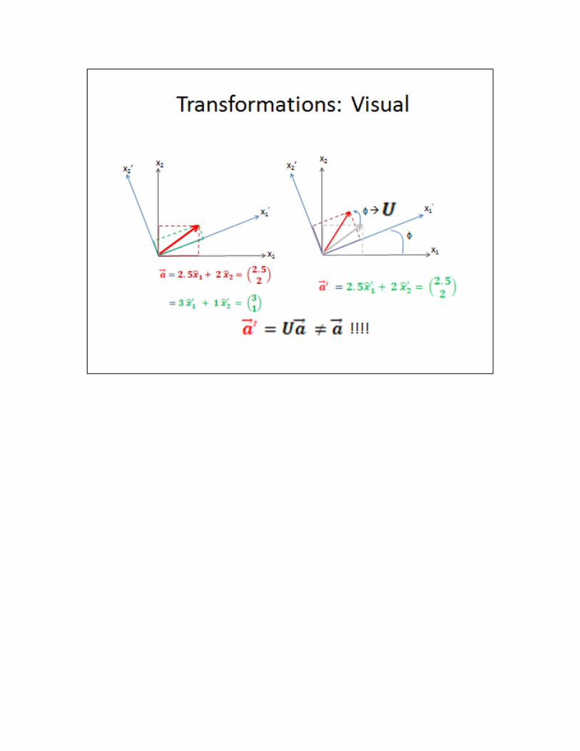
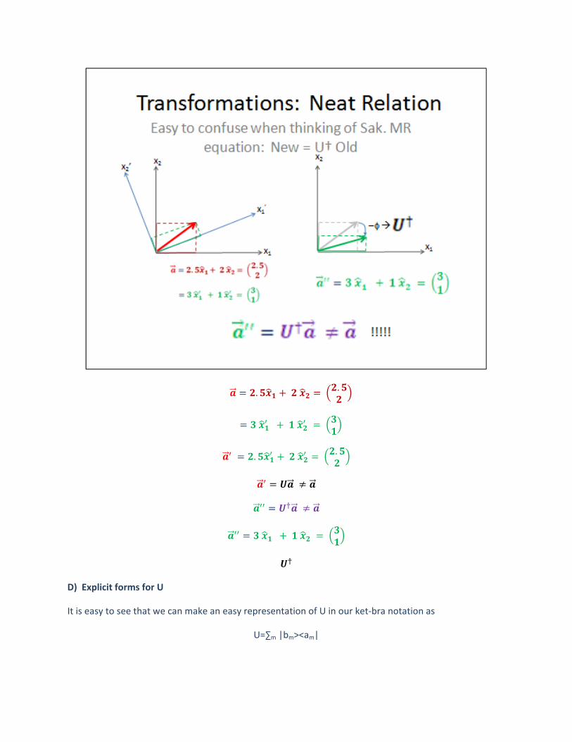
D)  Explicit forms for U 

It is easy to see that we can make an easy representation of U in our ket‐bra notation as  

U=∑m |bm><am| 

where |bm>  is the basis one may have the expansion of some vector |α> in, and |am> is the new basis.  

(obviously we could replace |b> by any other orthonormal basis that spans the same space).    

Also as with the matrix representation, such an explicit representation for a unitary operator only 

applies to discrete kets.  (discrete summation) 

  It is very easy to construct U† and prove that UU†  = 1. 

You see again, although U has the above simple form, to find the matrix elements of U in either basis 

e.g. in |a>   <an|U|am>  it will be necessary to know the expansion of |b> in the |a> basis, so it is 

perhaps good to think of the above simple form of U as really 

U=∑m (∑n [cm]n |an>)<am| 

or something similar with only |bm><bn|  outer products in it. Thus notice despite the original nice 

compact form of U, we still haven’t magically gotten away from this problem of having to find the group 

of numbers[ cm]n to specify it. 

 

Not to be confused with the completeness operator as described above:   

 1 =∑m |am><am|  =∑m |bm><bm| 

 

E)  Matrix Representations  and U (see above diagram) 

Hopefully I’ve convinced you that U acting on a ket will never just give us the expansion in another basis.  

Neither will U† .   However you will notice that Sakurai seems to concentrate on something that sounds 

similar:   that  

one can get the MATRIX REPRESENTATION of an arbitrary state |α> in the NEW BASIS by 

multiplying the MATRIX REPRESENTATION of U† in the OLD BASIS by the MATRIX 

REPRESENTATION of |α> in the OLD BASIS.     ‐‐(proper statement) 

For example  on page 38 he writes eq. (1.5.11):   (New) = U† (Old) 

It is of extreme importance that you do NOT interpret this as   

|new basis ket>  = U† |old basis ket>    (NO!!!!!) 

Such an interpretation isn’t at all true.  In fact, we stated that |b> = U|a>  and |b>’s where the “new 

basis ket’s”.  So at best this relation would be “backwards” if interpreted this way.  It can in fact only be 

interpreted as my “proper statement” above.   This is perhaps the clearest case that can distinguish our 

“pneumonic” from the real matrix representations—it is something that only makes sense for the 

FORMAL matrix representations of the kets, not for the kets themselves. 

As long as this is clear, then I will finally state that, yes, there is something else we can use U for in 

MATRIX REPRESENTATIONS, if we already have U’s own matrix representation defined, that is,  all its 

matrix elements are calculated.   It is just what we started out saying about how the ingredients of U  

Umn were related to the expansion of |b> in the basis |a>.    

 So we can think of the “other use” as the inverse relation of this:  if have the matrix element numbers 

Umn already, we actually have a convenient formula that Sakurai shows, for the projections of an 

arbitrary state |α> onto the new basis states <b|α> in terms of the old projections,  <a|α> 

<bn|α> = ∑n U†nm<am|α> 

Notice once more: it is nothing like U operating on |α>. The U†mn’s  are indeed pure numbers – in fact 

since matrix A† = AT* we can actually write these numbers more explicitly as (Umn)*   (note the ordering 

of the indices switched >transpose).  All we have really done here is taken our original expansion, bra‐

ed it to the right, and then taken the c.c. of both sides! 

‐‐‐‐ 

As it is just the uses of the numbers Unm that Sakurai concentrates on, it should now be clear that the in 

the sub section where he discusses how to find these numbers using the standard methods from linear 

algebra, the point is not HOW one does it (since we should already know this from linear algebra), but 

rather THAT one needs to do it, despite the convenient ket‐bra sum explicit form that was already given. 

 

F)  Unitary Equivalent Observables 

A and the operator UAU† are said to be unitary equivalent observables/operators.    It does NOT mean 

they are equal!!!   If you are trying to diagonalize A then UAU† will be diagonal but there will be other 

cases where will want to consider unitary equivalent observables/operators O where UOU†  (nor O) are 

diagonal.  

 

 

 

 

 

 

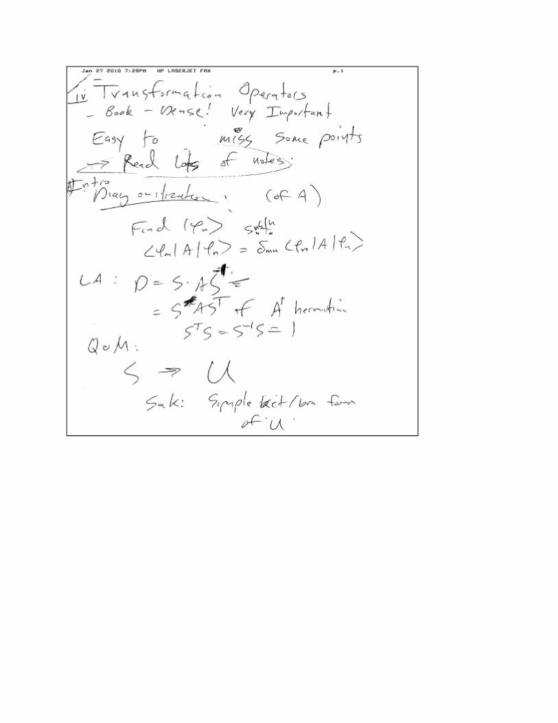
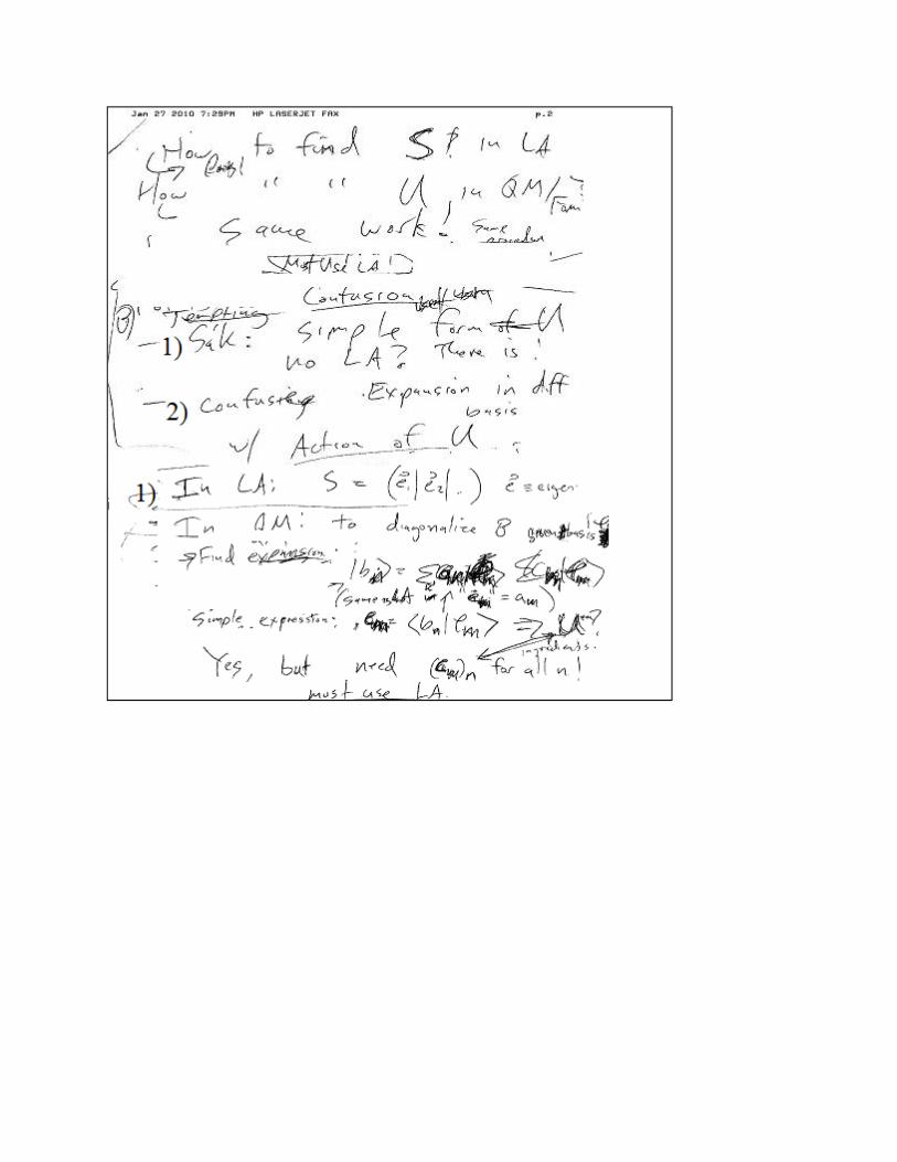
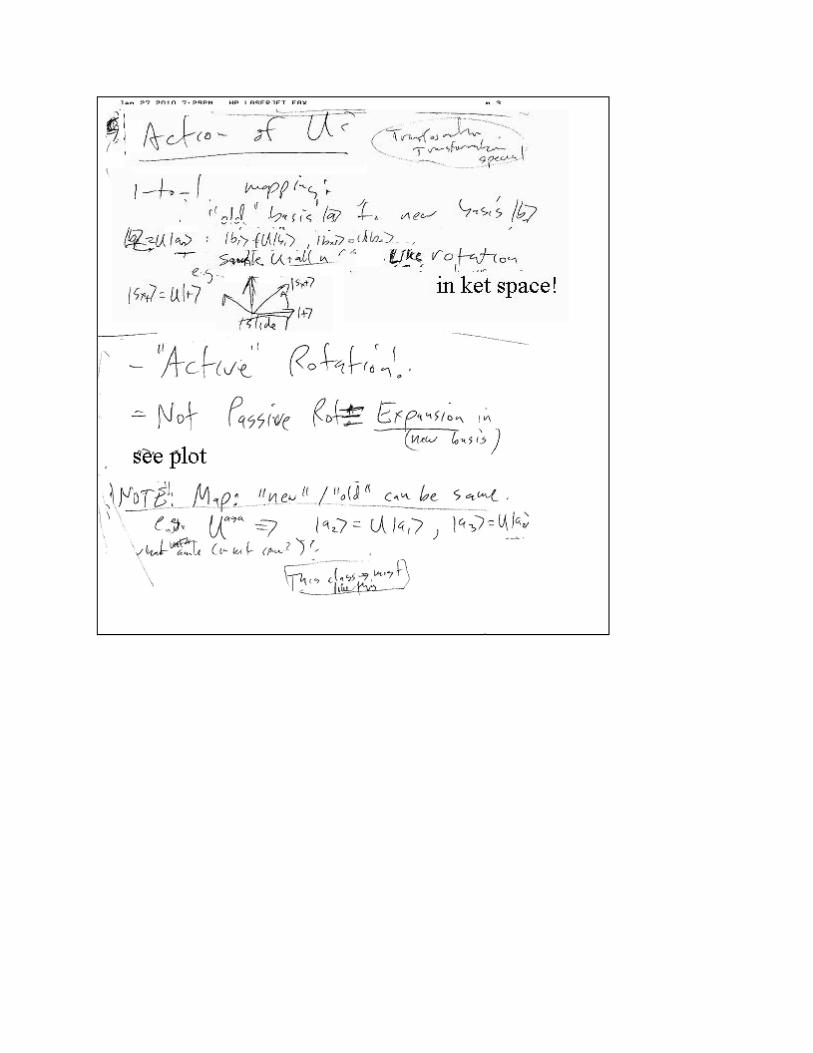
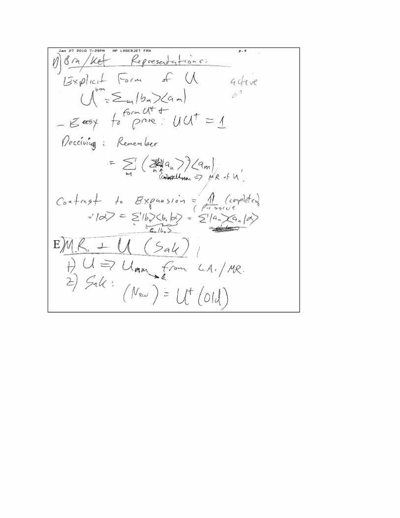
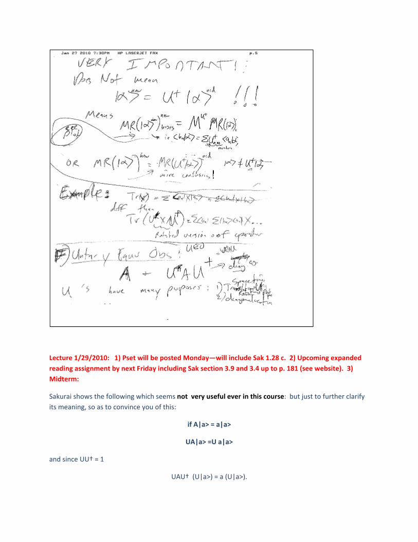
Lecture 1/29/2010:   1) Pset will be posted Monday—will include Sak 1.28 c.  2) Upcoming expanded 

reading assignment by next Friday including Sak section 3.9 and 3.4 up to p. 181 (see website).  3) 

Midterm:   

Sakurai shows the following which seems not  very useful ever in this course:  but just to further clarify 

its meaning, so as to convince you of this: 

if A|a> = a|a>   

UA|a> =U a|a> 

and since UU† = 1   

UAU†  (U|a>) = a (U|a>). 

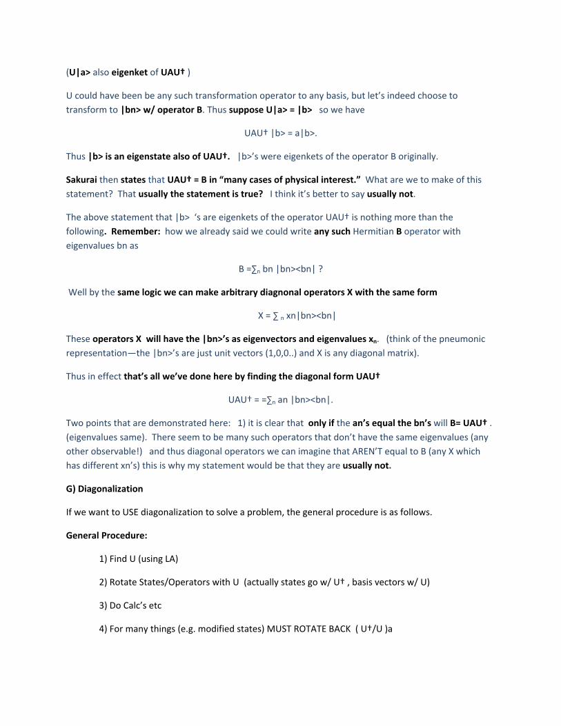
(U|a> also eigenket of UAU† )  

U could have been be any such transformation operator to any basis, but let’s indeed choose to 

transform to |bn> w/ operator B. Thus suppose U|a> = |b>   so we have   

UAU† |b> = a|b>. 

Thus |b> is an eigenstate also of UAU†.   |b>’s were eigenkets of the operator B originally.     

Sakurai then states that UAU† = B in “many cases of physical interest.”  What are we to make of this 

statement?  That usually the statement is true?   I think it’s better to say usually not.  

The above statement that |b>  ‘s are eigenkets of the operator UAU† is nothing more than the 

following.  Remember:  how we already said we could write any such Hermitian B operator with 

eigenvalues bn as    

B =∑n bn |bn><bn| ? 

 Well by the same logic we can make arbitrary diagnonal operators X with the same form  

X = ∑ n xn|bn><bn|  

These operators X  will have the |bn>’s as eigenvectors and eigenvalues xn.   (think of the pneumonic 

representation—the |bn>’s are just unit vectors (1,0,0..) and X is any diagonal matrix). 

Thus in effect that’s all we’ve done here by finding the diagonal form UAU†   

UAU† = =∑n an |bn><bn|. 

Two points that are demonstrated here:   1) it is clear that  only if the an’s equal the bn’s will B= UAU† .   

(eigenvalues same).  There seem to be many such operators that don’t have the same eigenvalues (any 

other observable!)   and thus diagonal operators we can imagine that AREN’T equal to B (any X which 

has different xn’s) this is why my statement would be that they are usually not. 

G) Diagonalization 

If we want to USE diagonalization to solve a problem, the general procedure is as follows. 

General Procedure:   

1) Find U (using LA)   

2) Rotate States/Operators with U  (actually states go w/ U† , basis vectors w/ U) 

3) Do Calc’s etc 

4) For many things (e.g. modified states) MUST ROTATE BACK  ( U†/U )a 

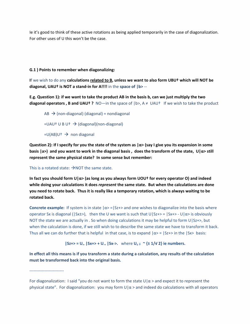
Ie it’s good to think of these active rotations as being applied temporarily in the case of diagonalization. 

For other uses of U this won’t be the case. 

 

 

G.1 ) Points to remember when diagonalizing:   

If we wish to do any calculations related to B, unless we want to also form UBU† which will NOT be 

diagonal, UAU† is NOT a stand‐in for A!!!! in the space of |b> ‐‐  

E.g. Question 1): if we want to take the product AB in the basis b, can we just multiply the two 

diagonal operators , B and UAU† ?  NO—in the space of |b>, A ≠  UAU†   If we wish to take the product 

AB   (non‐diagonal) (diagonal) = nondiagonal 

=UAU† U B U†   (diagonal)(non‐diagonal)  

=U(AB)U†    non diagonal 

Question 2): If I specify for you the state of the system as |α> (say I give you its expansion in some 

basis |a>)  and you want to work in the diagonal basis ,  does the transform of the state,  U|α> still 

represent the same physical state?  In some sense but remember: 

This is a rotated state: NOT the same state. 

In fact you should form U|α> (as long as you always form UOU† for every operator O) and indeed 

while doing your calculations it does represent the same state.  But when the calculations are done 

you need to rotate back.  Thus it is really like a temporary rotation, which is always waiting to be 

rotated back. 

Concrete example:  If system is in state |α> =|Sz+> and one wishes to diagonalize into the basis where 

operator Sx is diagonal (|Sx±>),   then the U we want is such that U|Sz+> = |Sx+> ‐ U|α> is obviously 

NOT the state we are actually in . So when doing calculations it may be helpful to form U|Sz+>, but 

when the calculation is done, if we still wish to to describe the same state we have to transform it back.  

Thus all we can do further that is helpful  in that case, is to expand |α> = |Sz+> in the |Sx>  basis:  

|Sz+> = U+‐ |Sx+> + U‐+ |Sx‐>.   where U±    ~ {± 1/√ 2} ie numbers. 

In effect all this means is if you transform a state during a calculation, any results of the calculation 

must be transformed back into the original basis. 

‐‐‐‐‐‐‐‐‐‐‐‐‐‐‐‐‐‐‐‐‐‐‐‐‐ 

For diagonalization:  I said “you do not want to form the state U|α > and expect it to represent the 

physical state”.  For diagonalization:  you may form U|α > and indeed do calculations with all operators 

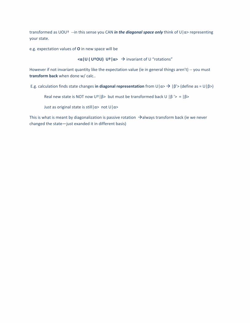
transformed as UOU†  ‐‐in this sense you CAN in the diagonal space only think of U|α> representing 

your state. 

e.g. expectation values of O in new space will be  

<α|U ( U†OU)  U†|α>    invariant of U “rotations” 

However if not invariant quantity like the expectation value (ie in general things aren’t) ‐‐ you must 

transform back when done w/ calc..  

 E.g. calculation finds state changes in diagonal representation from U|α>  |β’> (define as = U|β>)  

Real new state is NOT now U†|β>  but must be transformed back U |β ‘>  = |β> 

Just as original state is still|α>  not U|α>      

This is what is meant by diagonalization is passive rotation  always transform back (ie we never 

changed the state—just exanded it in different basis) 

 

 

   

Add example here:  3‐D?    2 pset examples.  Better examples for time dependence… 

 

IV Position And Momentum In the Formalism 

Introduction 

Sakurai sections 1.6‐7 tells us how to fit wave mechanics into our bra‐ket formalism.    The key point is 

that the basis we will use for the position operator |x> will be our type of continuous kets. 

One thing we never discussed: was summing up probabilities for multiple eigenvalues.  We said our 

measurement probability for discrete or continuous kets would be  

P(an)     |<an|α>|2 

First though consider that by definition the probability of getting one of a group of an values (3,4,5) 

would just be the sum of all probabities. 

 

P(an)     |<an|α>|2 P(an one of {a3, a4, a5}) =   ∑ n=3 to 5 |<an|α>|

2 

Actually this statement we need to clarify slightly for continuous kets |ξ>:.   

 For our continous kets, just as we initially defined them, to make linear combinations of these we need 

to integrate over our basis labels: e.g. for some random |ϕ > (like |α>) 

|ϕ >  = ∫ c(ξ) dξ |ξ> 

where obviously by completeness c(ξ) = <ξ|ϕ >.  In this expression we never specified what the 

integration limits ? were:  they could be over any range of ξ in fact, even   ∞  (∞  . . completeness).  

Suppose |ξ > is an eigenvector of some operator  ̂ s : then it should be easy to guess that  when trying 

to find the probability given a state |ϕ >that ξ will be is in some range ξ 1 ‐ ξ 2  when measured, we just 

integrate the over that range. 

1   2 | |   | | |  

 

A) Position Operators and Eigenkets 

For position : we will formally define the 

position operator in 1‐D :   x  

and 

 its eigenkets:  as continuous kets |x>. 

Thus all of what we described as ξ will apply for x:  Reminder:  all the definitions/rules apply except 

with an integral sign, in place of summation such as completeness. 

A word about completeness:  In fact we postulate that |x> forms a complete basis, which certainly 

makes sense: considering that we allow all x values from +/‐ infinity.   

However one might wonder as per our statements regarding the fact that as continuous kets |x> has an 

infinite norm and in fact we said that the ket |x> by itself is not a proper member of a genuine Hilbert 

space, whether this is “technically true”.  (infinite normnot proper Hilbert space members?)  ‐  

The answer is yes:  the eigen‐differentials we discussed that where the actual Hilbert space member, 

must satisfy a completeness relations, and we will assume that this completeness relation can be 

rewritten ∫ |x><x| dx 

Note that since the operator x should have only real eigenvalues, then by definition we must force it to 

be  hermitian.   x = x†  

Following  our expression for probability of continuous kets,  having in mind the probability for the 

eigenvalue x to be found in some range (x1, x2)—we know the expression will be  

1   2 | |  

were |c(x)|2 = |<x|α>|2 if the system is in the state |α>. 

Looking back to our wave mech review we can see that it appears that the projection of |α> on to the 

ket |x> must be the wave function ψ(x) from wave mechanics!! 

<x|α> = ψ α (x) 

If we like, we can extend the concept to 3 D:, defining such operators for each space dimension, x, y, z.   

These will have the same properties as for x (e.g. hermitian) 

We will say these three operators are all inter‐compatible so they commute [x,y] = [y,z] =[z,x] = 0.   

Thus they will have simultaneous eigenkets, |Pos>  

x|Pos> = xPos|Pos>,   y |Pos> = ypos |Pos>, z… 

 which would naturally be infinitely degenerate! for each value of 1 dimension   (in the other 2 

dimensions for any value for the 3rd.  ( Now one will note our discussions of degeneracies so far were 

only involving discrete kets.   We won’t discuss resolving continuous ket degeneracies. ) 

Thus we will label the 3‐D ket |x, y, z>  or better | >.    

The 3‐D wave function will then turn out to be the projection of the state |α> onto this 3‐D ket. 

< |α> = ψ α ( ) 

Because we will obviously want the probabibility of particle to be located in some 3‐D range {x1, x2:  y1, 

y2: z1,z2} as a triple integral 

| | |  

It is important (!) to realize that the 1‐D  x eigenket |x> is very different than the eigenket |x,y,z> even 

though both e.g. satisfy the eigenvalue equation. 

x|x’> = x’|x’>   &    x|x’,y’,z’> = x’|x’,y’,z’> 

 

Matrix Elements of Position Operators, and Functions thereof: 

 Remembering our norm for continuous kets:   <x|x’> = δ(x‐x’)  it is obvious that the 

Matrix element of x:    <x|x|x’>= x’ δ (x‐x’) 

which say means that it is “diagonal” just like if <n|A|m> = Anmδ mn.   

Similarly any operator which is a function f(x) of only the operator x (and no other operator)  

has a matrix element (in the position (==|x>) basis !) 

<x|f(x)|x’> = f(x’) δ (x‐x’) 

With this and in order to review many points at once, consider the general overlap integral expression 

for our expression of the projection of one ket state onto another (the inner product): 

 

In our wave mechanics review we said this projection  of state α onto state β was given by the integral  

∫ dx’ ψα*(x’)  ψ β (x’) 

Now it should be clear that in ket‐bra notation, this is exactly what is implied by the expression  <α|β>.  

So suppose |β > 

<α|β> where |β> = f(x)|β >   =  ?????  =  ∫ dx’ ψα*(x’) f(x’) ψ β (x’) 

We already described this integral in the wave mech review and described it as what <α|β> implies: 

Q: Why?  (<α |f(x)|β >   = <α| (∫ f(x) |x><x|β> ) 

Question:  what is the expectation value of x in a position eigenket? 

 

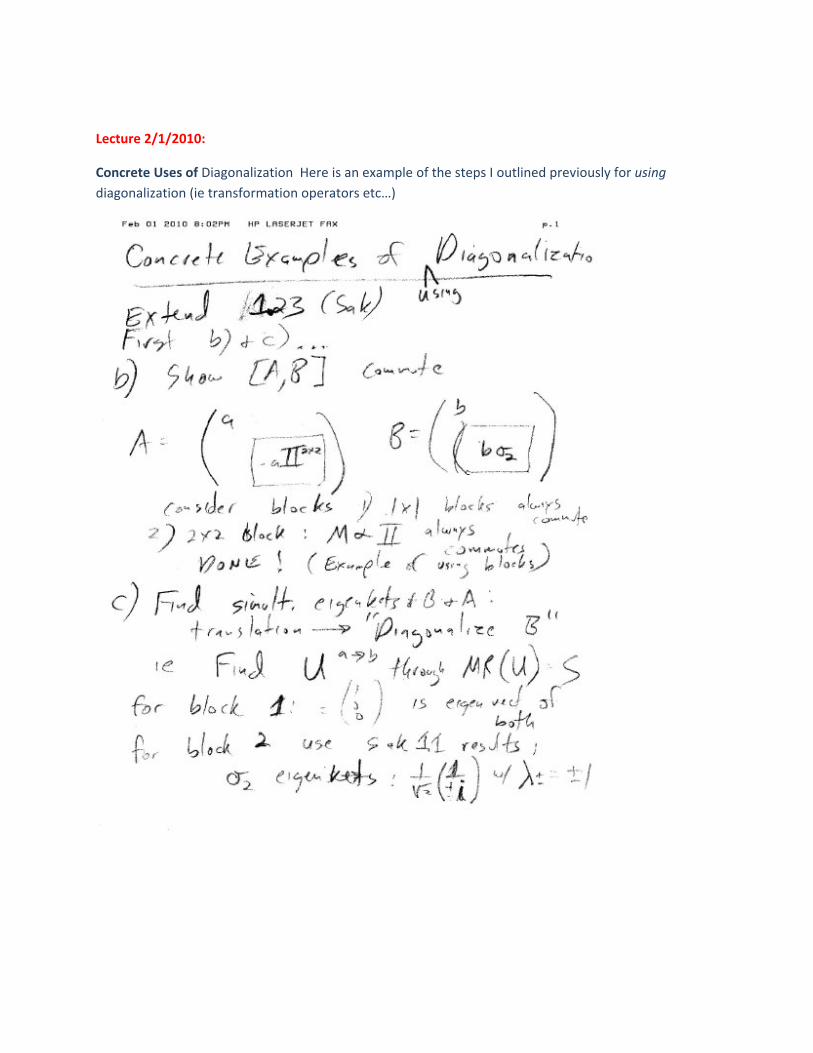
Lecture 2/1/2010:    

Concrete Uses of Diagonalization  Here is an example of the steps I outlined previously for using 

diagonalization (ie transformation operators etc…) 

 

 

 

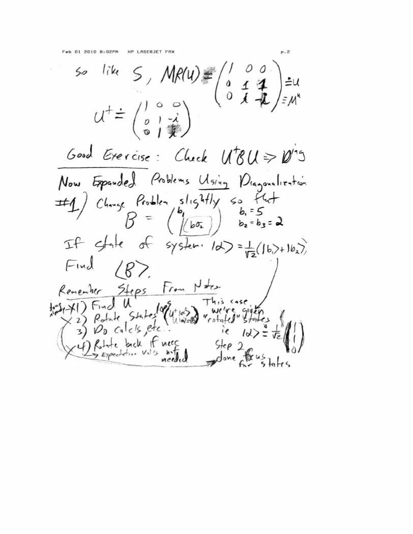
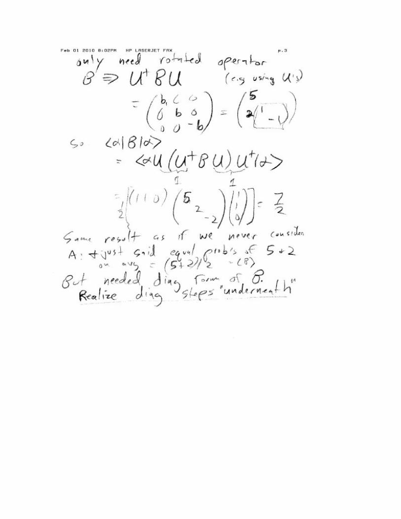
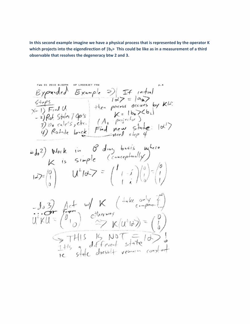
In this second example imagine we have a physical process that is represented by the operator K 

which projects into the eigendirection of |b2>  This could be like as in a measurement of a third 

observable that resolves the degeneracy btw 2 and 3. 

 

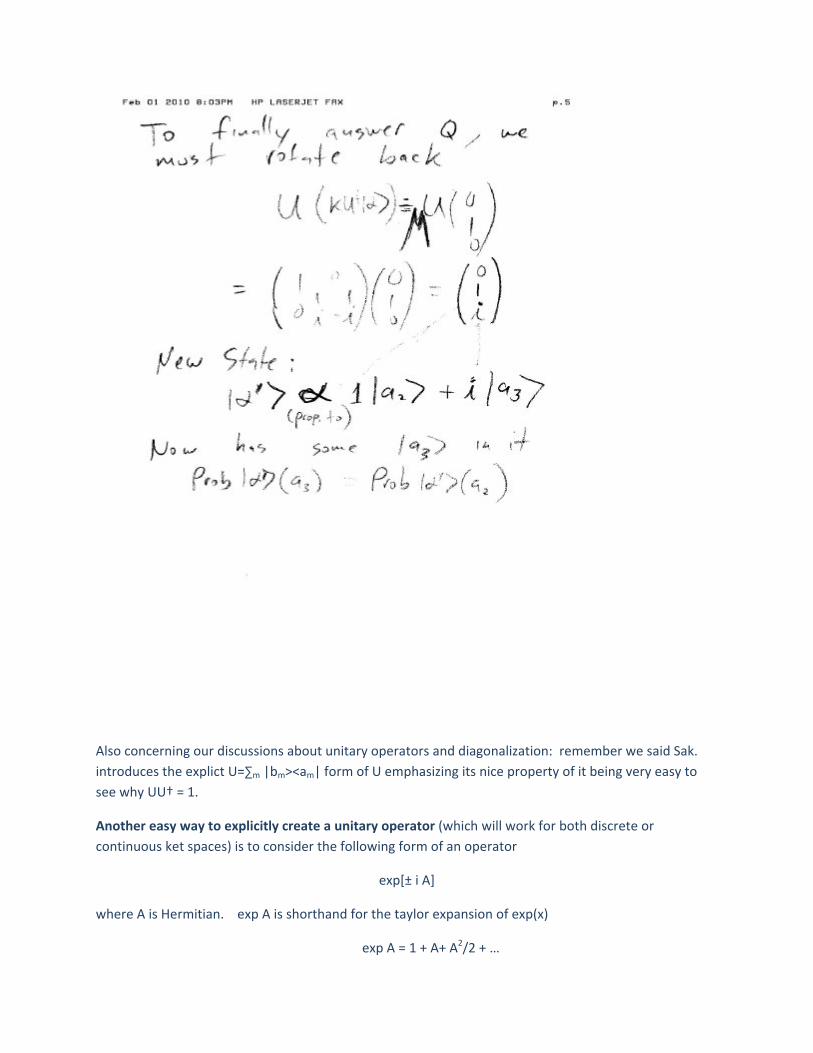
Also concerning our discussions about unitary operators and diagonalization:  remember we said Sak.  

introduces the explict U=∑m |bm><am| form of U emphasizing its nice property of it being very easy to 

see why UU† = 1. 

Another easy way to explicitly create a unitary operator (which will work for both discrete or 

continuous ket spaces) is to consider the following form of an operator 

exp[± i A] 

where A is Hermitian.    exp A is shorthand for the taylor expansion of exp(x)   

exp A = 1 + A+ A2/2 + … 

And it is easy to see that these “exponentiated operators” obey our normal expectations for 

exponentiated numbers.  e.g. since  exp(‐A) = 1 – A + A2/2+…       

exp(‐A) exp A = (1 +A –A + A2 – A*A + …) = 1 

It is easy to see therefore that  (exp[± i A])† = exp[ iA]  for as long as A is hermitian, we only need to 

take the complex conjugate of i.   And thus we have the required U†U = 1. 

For problem 1.28 you want to do an expansion like this, and simply apply the following commutation 

relation [x,px] =i   which we will prove early next week.  Purely algebraic problem you can already do 

using these simple algebraic relations.  (another hint—start with finding what [x,px] = i   implies for 

[x,pxn]) 

 

B)   The Translation and Momentum Operators 

In Sakurai 1.6 we see the first of several instances of introducing important operators through the role 

they play in very fundamental Transformation Operators  U  that we discussed in the last section.    How fundamental?  These Transformation Operators will always correspond to some symmetry of 

space‐time itself!      

In this case we will introduce the momentum operator through the fundamental transformation of 

Space translation:  

Comments:  Notice that in choosing our definition of base kets |x> we considered any no certain 

situation, like in the case of spin, where we had the results of the SG experiment in mind.  Thus as is 

implied by their simple labels they should somehow be dependent only on the properties of space 

itself, not e.g. of any particular energy configuration or Hamiltonian.   

As we can move around in space, we expect there to be a unitary transf. operator that can take us 

from one location’s ket |x1> to another |x2> 

In ket space this is a rotation of (Q how many? 90) degrees in 1 special direction.   In terms of the real 

space we can consider this a translation:   

if x2‐x1 = a (some constant) 

then we will call such a translation transformation operator  T12   so that we have  

|x2> = |x1+a> = T12 |x1> 

Suppose we consider a T which does the exact same translation operation for any value of x:   T ↔  

T(a), not just |x1>  |x2>. 

If this is the case, besides automatically needing this to be a Unitary operator (as all such transformation 

operators must) 

T† T = 1 

we expect (require!) this T to follow all our intuitions about  translations in space: 

1.  Successive translations:   T(a)T(b)|x>  = T(a+b)|x> 

2.) Inverse same as opposite direction translation  T(‐a) = T‐1(a) = T†(a) 

3)  If the translation a  0  it should become the identity operator lima→0T(a) = 1 

 

Especially because of 1 we should immediately think of exponentiation  : zazb = za+b 

And indeed the other 2 requirements along conveniently with the unitary requirement all at once with 

an operator of the form we discussed last time: 

T(a) = exp(± ika)  where k could be ANY hermitian operator!   

We will choose exp(‐ika)  ‐‐ reasons will be obvious 

 

Lecture 2/2/2010 

 

Although any operator k will satisfy the necessary properties (1,2,3 and Unitarity) we want of the 

translation operator, something else special will be required of how the operator k acts on the position 

kets |x> in order to actually accomplish the real ket translation we want: 

|x1+a> = T(a)|x1> 

All that’s required : for this however is that k must obey the following commutation relation with the x 

operator:   

[x,k] = i 

That this commutation relation works is proven in your homework (we will prove later that k   p. 

   

That this commutation relation works is proven in your homework (we will prove later that k   p),  but 

let’s mention how Sak proves it.  He considers infinitesimal translations T(ϵ) 

Remembering “dx’” is just a number!  I prefer to use the more usual convention for such a small 

numberϵ  

see that exp(ikϵ) in that case can just be reduced to 

T(ϵ) ≈ 1‐ikϵ 

since we can ignore any term of order in epsilon  of ϵ 2 or higher in comparison to ϵ itself.  This is 

extremely convenient—any time we see a term of ϵ 2 or higher we can simply cancel it immediately.  

Further, we see that our posited commutation relation  [x,k] = i will imply that  

[x,k] = i    [x,T(ϵ)] =  ϵ 

Q why?  

Using these we apply T(ϵ) to |x’> and operate on it with the  position operator   

x (T(ϵ) |x’>) = (T(ϵ)x + [x,T(ϵ)])|x’> 

imagine if [x,T(ϵ)] = ϵ

= (T(ϵ)x + ϵ|x’> 

but to this we can add any term   ϵ2 without penalty do so,  in the form of ikϵ2|x’> 

 x’T( ϵ) + ϵ+ ikϵ2 |x’>   = (x’+ϵ ) |x’>  + iϵ k |x’> 

= x’T( ϵ)  + ϵ(1 +ikϵ)|x’> 

= (x’+ϵ ) T(ϵ)|x’> 

Notice that it is such a manipulation that justifies line Sakurai 1.6.24: 

[T(ϵ),x] |x’> = ϵ |x+ϵ >   ϵ |x> 

Not some kind of Taylor expansion of |x+ϵ>  : One cannot Taylor expand one basis state in terms of 

others!!!     

Q:  Why?  (operators OK, not orthogonal kets)  

 

So we have what we set out to get— 

x(T(ϵ)|x’>)  = (x’+ϵ ) T(ϵ)|x’>    that is,  T(ϵ)|x’> is an eigenket of the operator x, with eigenvalue  (x’+ϵ ). 

Thus it must be what we call the ket  |x’+ϵ >  or at least proportional to it.  (ie T(ϵ)|x> = const x|x+ϵ>)  

Apparently following Sakurai we will choose this constant to be 1 (remember we already said these 

kets have INFINITE NORM anyways).   And thus 

T(ϵ)|x’> = |x’+ϵ > 

SUCH A CONCLUSION WILL BE USED MANY TIMES IN THIS COURSE—GET USED TO USING IT! : if  we have 

B (A|b1>) = b2 (A|b1>)   we will always say  A|b1> must = c|b2> where c is some numerical constant. 

Our translation operator does what we wanted.  So you see it is just a simple algebraic relation that 

allows for this.   

 

 

Why k is proportional to the momentum 

It turns out that we can identify k as being proportional to the momentum of the particle.  To see how 

this comes about, it is instructive to observe its matrix element  

Look at the wave function of the state  

|α’> = T(ϵ ) |α>     <x’|α’> = ψ α’ (x) = <x’| T(ϵ) |α>  

<x’| T(ϵ) |α>  =   <x’| T(ϵ) |α> 

(2‐side  Parallel ) 

LHS:   By our properties of      T(ϵ) = T†(‐ϵ) 

= [ <x’|T† (‐ϵ) ]  |α> = <x‐ϵ|α> = ψα (x‐ϵ) 

 Taylor expansion in ϵ  

 

For RHS: 

T(ϵ) ≈ 1‐ikϵ T(ϵ) = exp(‐ikϵ) =  1‐ikϵ+1/2 (ikϵ)2+…  

So we have <x’| T(ϵ)|α> 

= <x’| =  1‐ikϵ+1/2 (ikϵ)2+…|α> 

= 

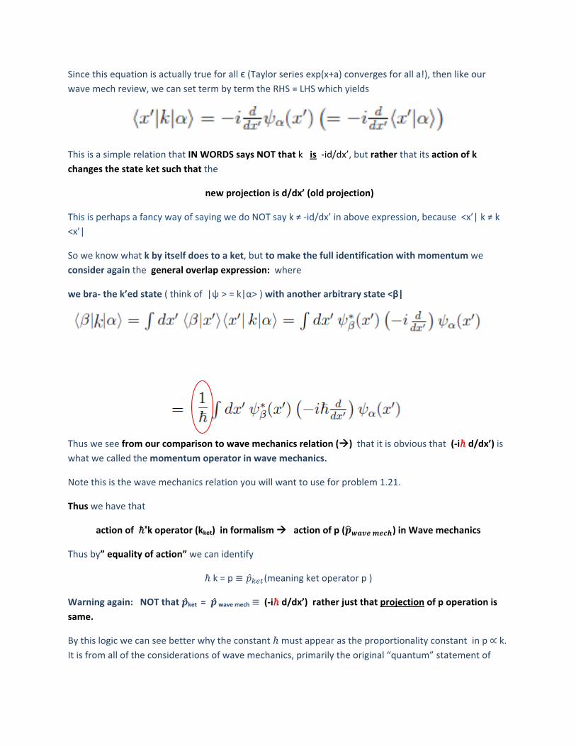
Since this equation is actually true for all ϵ (Taylor series exp(x+a) converges for all a!), then like our 

wave mech review, we can set term by term the RHS = LHS which yields 

 

This is a simple relation that IN WORDS says NOT that k   is  ‐id/dx’, but rather that its action of k 

changes the state ket such that the 

 new projection is d/dx’ (old projection) 

This is perhaps a fancy way of saying we do NOT say k ≠ ‐id/dx’ in above expression, because  <x’| k ≠ k 

<x’| 

So we know what k by itself does to a ket, but to make the full identification with momentum we 

consider again the  general overlap expression:  where  

we bra‐ the k’ed state ( think of  |ψ > = k|α> ) with another arbitrary state <β|  

 

 

 

 

Thus we see from our comparison to wave mechanics relation ()  that it is obvious that  (‐i  d/dx’) is 

what we called the momentum operator in wave mechanics. 

Note this is the wave mechanics relation you will want to use for problem 1.21.   

Thus we have that 

action of   xk operator (kket)  in formalism    action of p (   ) in Wave mechanics  

Thus by” equality of action” we can identify  

 k = p  ̂ (meaning ket operator p )  

Warning again:   NOT that  ̂ket  =    ̂wave mech    (‐i  d/dx’)  rather just that projection of p operation is 

same. 

By this logic we can see better why the constant   must appear as the proportionality constant  in p   k.  

It is from all of the considerations of wave mechanics, primarily the original “quantum” statement of  

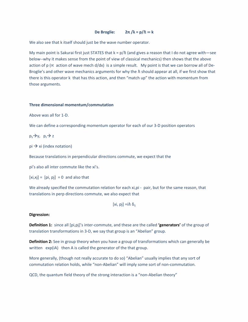
De Broglie:          2π /λ = p/    k  

We also see that k itself should just be the wave number operator. 

My main point is Sakurai first just STATES that k = p/  (and gives a reason that I do not agree with—see 

below‐‐why it makes sense from the point of view of classical mechanics) then shows that the above 

action of p (   action of wave mech d/dx)  is a simple result.   My point is that we can borrow all of De‐

Broglie’s and other wave mechanics arguments for why the   should appear at all, if we first show that 

there is this operator k  that has this action, and then “match up” the action with momentum from 

those arguments. 

 

Three dimensional momentum/commutation 

Above was all for 1‐D. 

We can define a corresponding momentum operator for each of our 3‐D position operators 

pyy,   pz z 

pi  xi (index notation) 

Because translations in perpendicular directions commute, we expect that the  

pi’s also all inter commute like the xi’s. 

[xi,xj] =  [pi, pj]  = 0  and also that  

We already specified the commutation relation for each xi,pi ‐  pair, but for the same reason, that 

translations in perp directions commute, we also expect that  

[xi, pj] =i  δij 

Digression:   

Definition 1:  since all [pi,pj]’s inter‐commute, and these are the called ‘generators’ of the group of 

translation transformations in 3‐D, we say that group is an “Abelian” group.     

Definition 2: See in group theory when you have a group of transformations which can generally be 

written   exp(iA)   then A is called the generator of the that group. 

More generally, (though not really accurate to do so) “Abelian” usually implies that any sort of 

commutation relation holds, while “non‐Abelian” will imply some sort of non‐commutation.   

QCD, the quantum field theory of the strong interaction is a “non‐Abelian theory” 

 

Lecture 2/2/09 

Review 

reading assignment Sak 2.3 up to time dev of the oscillator. 

Question : True/False in the bra ket formalism is the operator p is ‐ih d/dx? 

For example, in Sak. 1.29  the relation:  Sak 1.29 [p,F(x)] = dF/dx   or [x,G(p) ]   

 you may remember from wave mech:  [introduce “test function”  pwave mech  = ihd/dx] 

The action of p => ihd/dx   NOT  pket = ihd/dx 

continuint from last time we said: 

[xi,xj] =  [pi, pj]  = 0  

We already specified the commutation relation for each xi,pi ‐  pair, but for the same reason, that 

translations in perp directions commute, we also expect that  

[xi, pj] =i  δij  

 

Relations to Classical Mechanics /Commutators 

Sakurai tries to justify k = p/  as a “trick of language”  

generator  <‐‐ > generating function 

The language makes sense especially in this case for because somehow in this case p/  is “responsible” 

for the translation action. 

But I do not think Sakurai’s analogy to the classical mechanics “Generating Function” is very intuitive.  

See my comment in the optional reading.    Just because they share the same root word “generate “ 

they are not very alike.    

Contrived:  means not something that would happens natural: but artificially prepared. 

Comment:  Often authors try in this way to point out similarities between Quantum and Classical 

mechanics as if to “it had to be that way” or “one can actually derive” Quantum Mechanics from 

Classical Mechanics” (?).  But this is not really the case.    

It wasn’t by observing these classical expressions and then magically forming the “quantum” equivalent  

and they saw it worked.   No it is the other way around.  We had to construct the quantum theory and 

all it’s weird conceptual implications first, with only very loose relations to classical mechanical 

concepts. (for example one loose relation that was used is to “insert”   ‘s in a way that in the limit of   

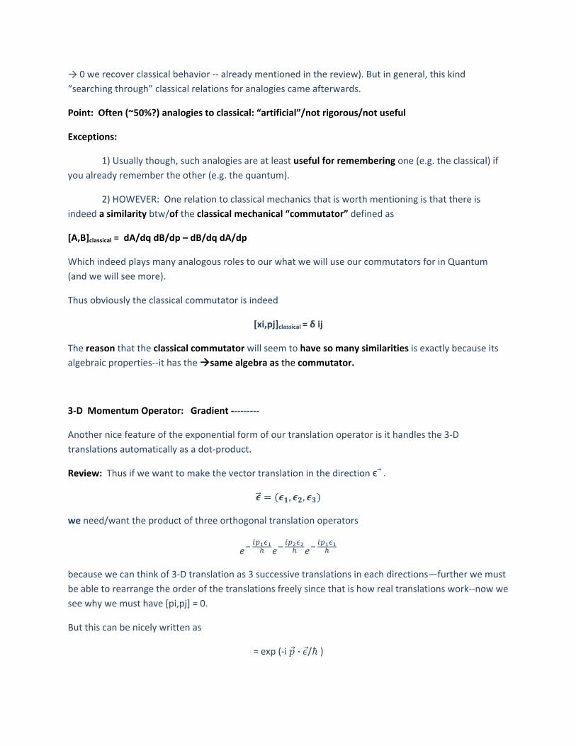
→ 0 we recover classical behavior ‐‐ already mentioned in the review). But in general, this kind 

“searching through” classical relations for analogies came afterwards. 

Point:  Often (~50%?) analogies to classical: “artificial”/not rigorous/not useful 

Exceptions:   

1) Usually though, such analogies are at least useful for remembering one (e.g. the classical) if 

you already remember the other (e.g. the quantum). 

2) HOWEVER:  One relation to classical mechanics that is worth mentioning is that there is 

indeed a similarity btw/of the classical mechanical “commutator” defined as 

[A,B]classical =  dA/dq dB/dp – dB/dq dA/dp 

Which indeed plays many analogous roles to our what we will use our commutators for in Quantum 

(and we will see more). 

Thus obviously the classical commutator is indeed  

[xi,pj]classical = δ ij 

The reason that the classical commutator will seem to have so many similarities is exactly because its 

algebraic properties‐‐it has the same algebra as the commutator. 

 

3‐D  Momentum Operator:   Gradient ‐‐‐‐‐‐‐‐‐ 

Another nice feature of the exponential form of our translation operator is it handles the 3‐D 

translations automatically as a dot‐product.   

Review:  Thus if we want to make the vector translation in the direction ϵ  . 

, ,  

we need/want the product of three orthogonal translation operators 

       

because we can think of 3‐D translation as 3 successive translations in each directions—further we must 

be able to rearrange the order of the translations freely since that is how real translations work‐‐now we 

see why we must have [pi,pj] = 0. 

But this can be nicely written as  

= exp (‐i  · /  ) 

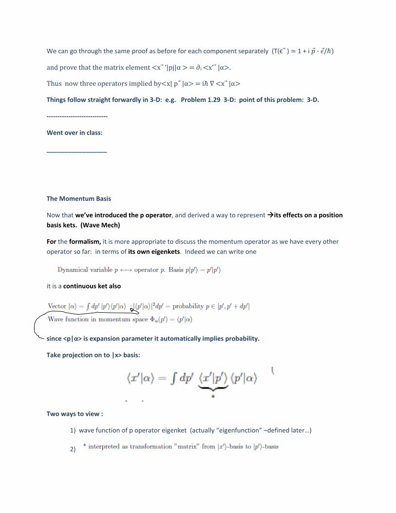
We can go through the same proof as before for each component separately  (T(ϵ  )   1 + i  · /  

and prove that the matrix element  x  ‘|pj|α      i  x’  |α .   

Thus  now three operators implied by x| p  |α    i     x  |α  

Things follow straight forwardly in 3‐D:  e.g.   Problem 1.29  3‐D:  point of this problem:  3‐D. 

‐‐‐‐‐‐‐‐‐‐‐‐‐‐‐‐‐‐‐‐‐‐‐‐‐‐‐‐ 

Went over in class:   

_________________ 

 

 

The Momentum Basis 

Now that we’ve introduced the p operator, and derived a way to represent its effects on a position 

basis kets.  (Wave Mech) 

For the formalism, it is more appropriate to discuss the momentum operator as we have every other 

operator so far:  in terms of its own eigenkets.  Indeed we can write one 

 

it is a continuous ket also  

 

since <p|α> is expansion parameter it automatically implies probability. 

Take projection on to |x> basis: 

 

Two ways to view :    

  1)  wave function of p operator eigenket  (actually “eigenfunction” –defined later…) 

  2)    

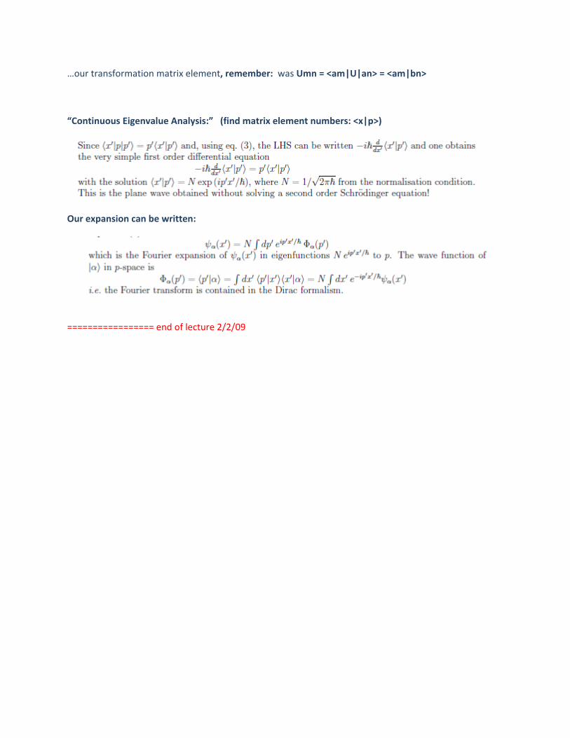
…our transformation matrix element, remember:  was Umn = <am|U|an> = <am|bn> 

 

“Continuous Eigenvalue Analysis:”   (find matrix element numbers: <x|p>) 

  

Our expansion can be written: 

 

================= end of lecture 2/2/09 

   

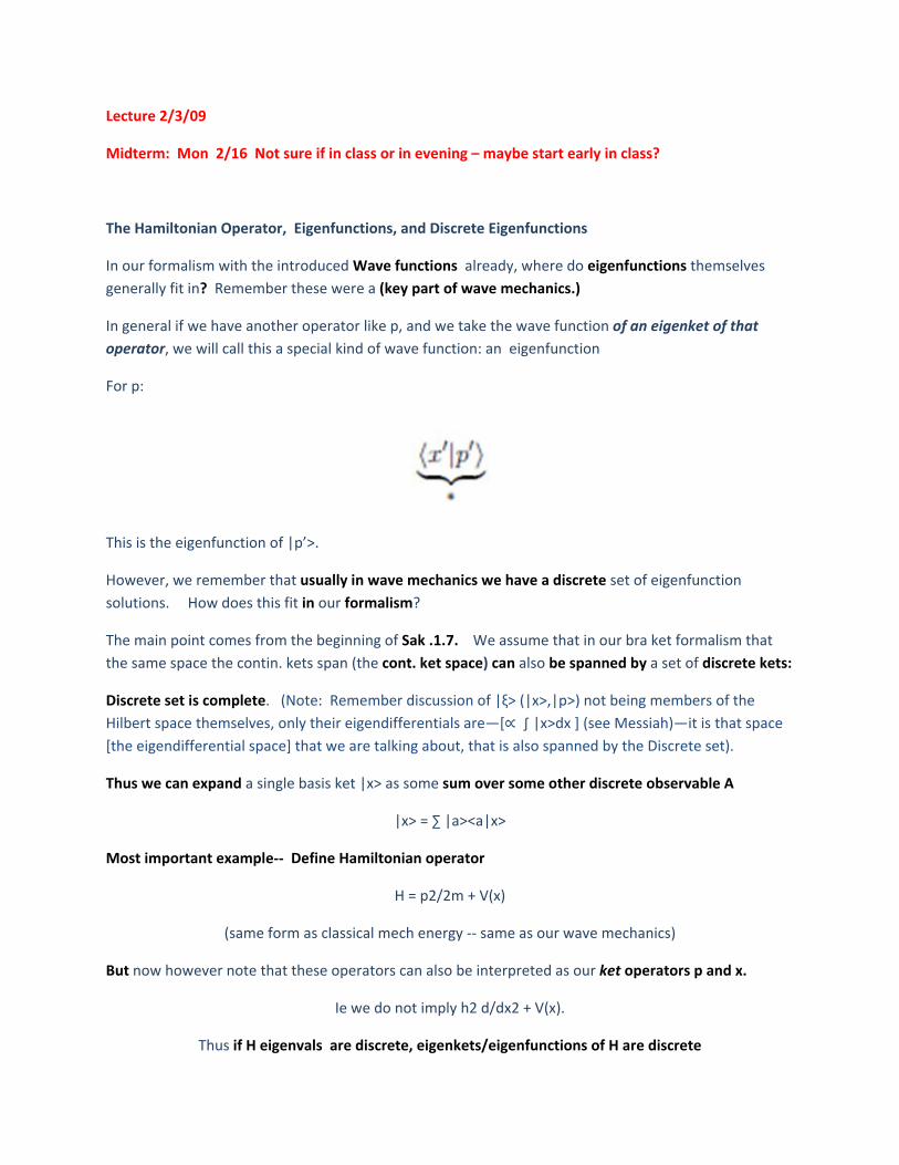
Lecture 2/3/09 

Midterm:  Mon  2/16  Not sure if in class or in evening – maybe start early in class? 

 

The Hamiltonian Operator,  Eigenfunctions, and Discrete Eigenfunctions 

In our formalism with the introduced Wave functions  already, where do eigenfunctions themselves 

generally fit in?  Remember these were a (key part of wave mechanics.) 

In general if we have another operator like p, and we take the wave function of an eigenket of that 

operator, we will call this a special kind of wave function: an  eigenfunction 

For p: 

 

This is the eigenfunction of |p’>. 

However, we remember that usually in wave mechanics we have a discrete set of eigenfunction 

solutions.     How does this fit in our formalism?  

The main point comes from the beginning of Sak .1.7.    We assume that in our bra ket formalism that 

the same space the contin. kets span (the cont. ket space) can also be spanned by a set of discrete kets: 

Discrete set is complete.   (Note:  Remember discussion of |ξ> (|x>,|p>) not being members of the 

Hilbert space themselves, only their eigendifferentials are—[   ∫ |x>dx ] (see Messiah)—it is that space 

[the eigendifferential space] that we are talking about, that is also spanned by the Discrete set). 

Thus we can expand a single basis ket |x> as some sum over some other discrete observable A 

|x> = ∑ |a><a|x> 

Most important example‐‐  Define Hamiltonian operator 

H = p2/2m + V(x) 

(same form as classical mech energy ‐‐ same as our wave mechanics) 

But now however note that these operators can also be interpreted as our ket operators p and x.  

Ie we do not imply h2 d/dx2 + V(x). 

Thus if H eigenvals  are discrete, eigenkets/eigenfunctions of H are discrete 

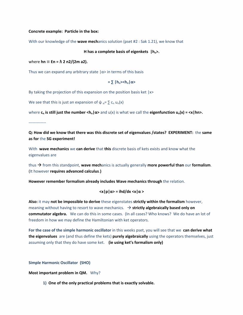
Concrete example:  Particle in the box:   

With our knowledge of the wave mechanics solution (pset #2 : Sak 1.21), we know that  

H has a complete basis of eigenkets  |hn>. 

where hn   En =   2 n2/(2m a2). 

Thus we can expand any arbitrary state |α> in terms of this basis 

= ∑ |hn><hn|α> 

By taking the projection of this expansion on the position basis ket |x> 

We see that this is just an expansion of ψ α= ∑ cn un(x) 

where cn is still just the number <hn|α> and u(x) is what we call the eigenfunction un(x) = <x|hn>. 

‐‐‐‐‐‐‐‐‐‐‐‐‐ 

Q: How did we know that there was this discrete set of eigenvalues /states?  EXPERIMENT:  the same 

as for the SG experiment! 

With  wave mechanics we can derive that this discrete basis of kets exists and know what the 

eigenvalues are 

thus  from this standpoint, wave mechanics is actually generally more powerful than our formalism. 

(It however requires advanced calculus.)   

However remember formalism already includes Wave mechanics through the relation.  

<x|p|α> = ihd/dx <x|α > 

Also: it may not be impossible to derive these eigenstates strictly within the formalism however, 

meaning without having to resort to wave mechanics.    strictly algebraically based only on 

commutator algebra.   We can do this in some cases.  (In all cases? Who knows?  We do have an lot of 

freedom in how we may define the Hamiltonian with ket operators.   

For the case of the simple harmonic oscillator in this weeks pset, you will see that we  can derive what 

the eigenvalues  are (and thus define the kets) purely algebraically using the operators themselves, just 

assuming only that they do have some ket.    (ie using ket’s formalism only) 

 

Simple Harmonic Oscillator  (SHO) 

Most important problem in QM.   Why? 

1)  One of the only practical problems that is exactly solvable. 

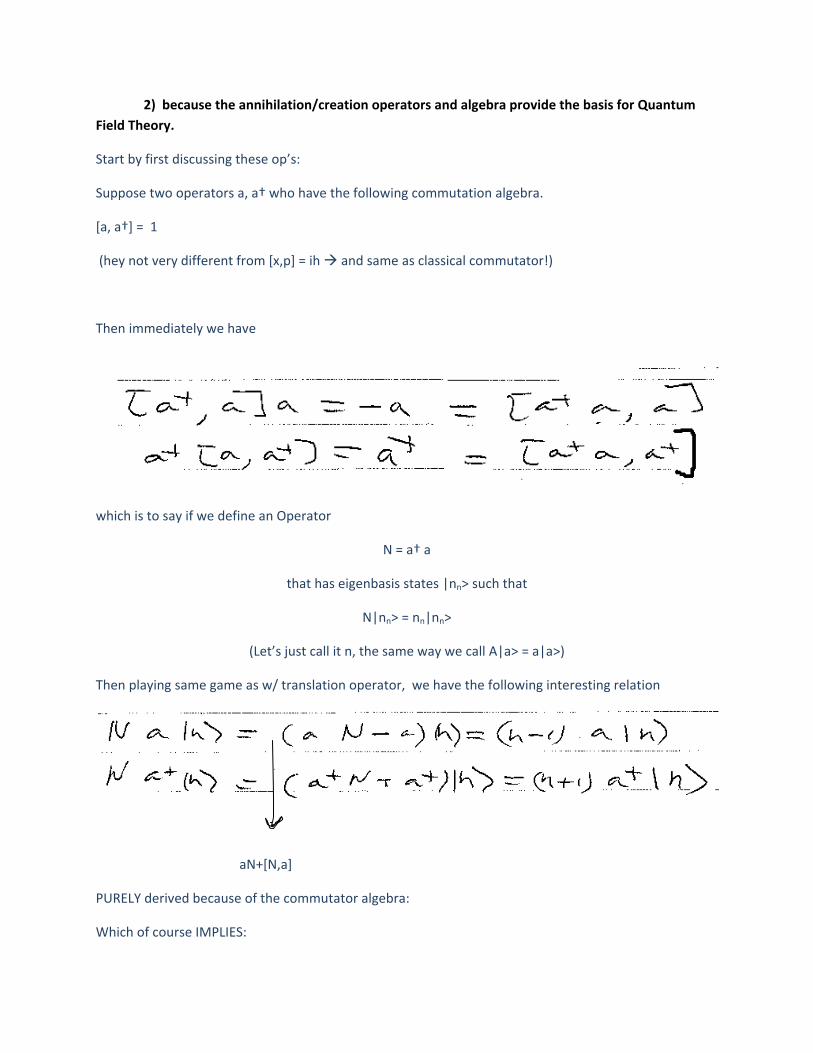
2)  because the annihilation/creation operators and algebra provide the basis for Quantum 

Field Theory.    

Start by first discussing these op’s: 

Suppose two operators a, a† who have the following commutation algebra.  

[a, a†] =  1   

 (hey not very different from [x,p] = ih  and same as classical commutator!) 

 

Then immediately we have 

 

which is to say if we define an Operator  

N = a† a 

that has eigenbasis states |nn> such that 

N|nn> = nn|nn> 

(Let’s just call it n, the same way we call A|a> = a|a>) 

Then playing same game as w/ translation operator,  we have the following interesting relation  

 

 

aN+[N,a]   

PURELY derived because of the commutator algebra:  

Which of course IMPLIES: 

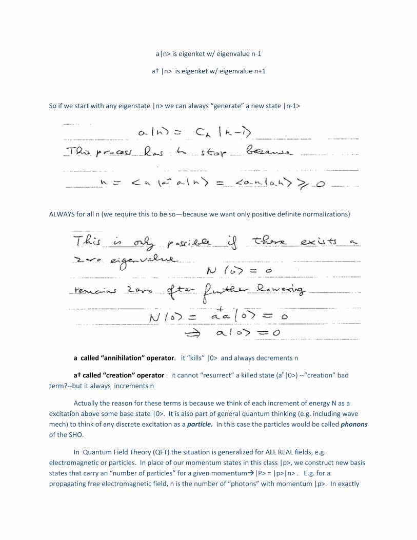
a|n> is eigenket w/ eigenvalue n‐1 

a† |n>  is eigenket w/ eigenvalue n+1 

 

So if we start with any eigenstate |n> we can always “generate” a new state |n‐1> 

 

ALWAYS for all n (we require this to be so—because we want only positive definite normalizations) 

 

a  called “annihilation” operator.   it “kills” |0>  and always decrements n  

a† called “creation” operator .  it cannot “resurrect” a killed state (an|0>) ‐‐“creation” bad 

term?‐‐but it always  increments n 

Actually the reason for these terms is because we think of each increment of energy N as a 

excitation above some base state |0>.  It is also part of general quantum thinking (e.g. including wave 

mech) to think of any discrete excitation as a particle.  In this case the particles would be called phonons 

of the SHO.   

In  Quantum Field Theory (QFT) the situation is generalized for ALL REAL fields, e.g. 

electromagnetic or particles.  In place of our momentum states in this class |p>, we construct new basis 

states that carry an “number of particles” for a given momentum|P> = |p>|n> .   E.g. for a 

propagating free electromagnetic field, n is the number of “photons” with momentum |p>.  In exactly 

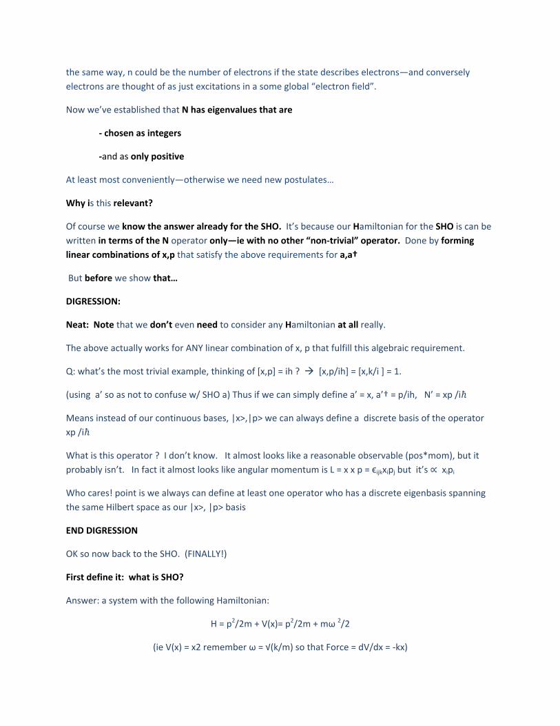
the same way, n could be the number of electrons if the state describes electrons—and conversely 

electrons are thought of as just excitations in a some global “electron field”. 

Now we’ve established that N has eigenvalues that are  

‐ chosen as integers 

‐and as only positive 

At least most conveniently—otherwise we need new postulates… 

Why is this relevant?    

Of course we know the answer already for the SHO.  It’s because our Hamiltonian for the SHO is can be 

written in terms of the N operator only—ie with no other “non‐trivial” operator.  Done by forming 

linear combinations of x,p that satisfy the above requirements for a,a†  

 But before we show that… 

DIGRESSION: 

Neat:  Note that we don’t even need to consider any Hamiltonian at all really.    

The above actually works for ANY linear combination of x, p that fulfill this algebraic requirement. 

Q: what’s the most trivial example, thinking of [x,p] = ih ?    [x,p/ih] = [x,k/i ] = 1. 

(using  a’ so as not to confuse w/ SHO a) Thus if we can simply define a’ = x, a’† = p/ih,   N’ = xp /i     

Means instead of our continuous bases, |x>,|p> we can always define a  discrete basis of the operator 

xp /i     

What is this operator ?  I don’t know.   It almost looks like a reasonable observable (pos*mom), but it 

probably isn’t.   In fact it almost looks like angular momentum is L = x x p = ϵijkxipj but  it’s    xipi 

Who cares! point is we always can define at least one operator who has a discrete eigenbasis spanning 

the same Hilbert space as our |x>, |p> basis    

END DIGRESSION 

OK so now back to the SHO.  (FINALLY!)   

First define it:  what is SHO? 

Answer: a system with the following Hamiltonian:   

H = p2/2m + V(x)= p2/2m + mω 2/2 

(ie V(x) = x2 remember ω = √(k/m) so that Force = dV/dx = ‐kx) 

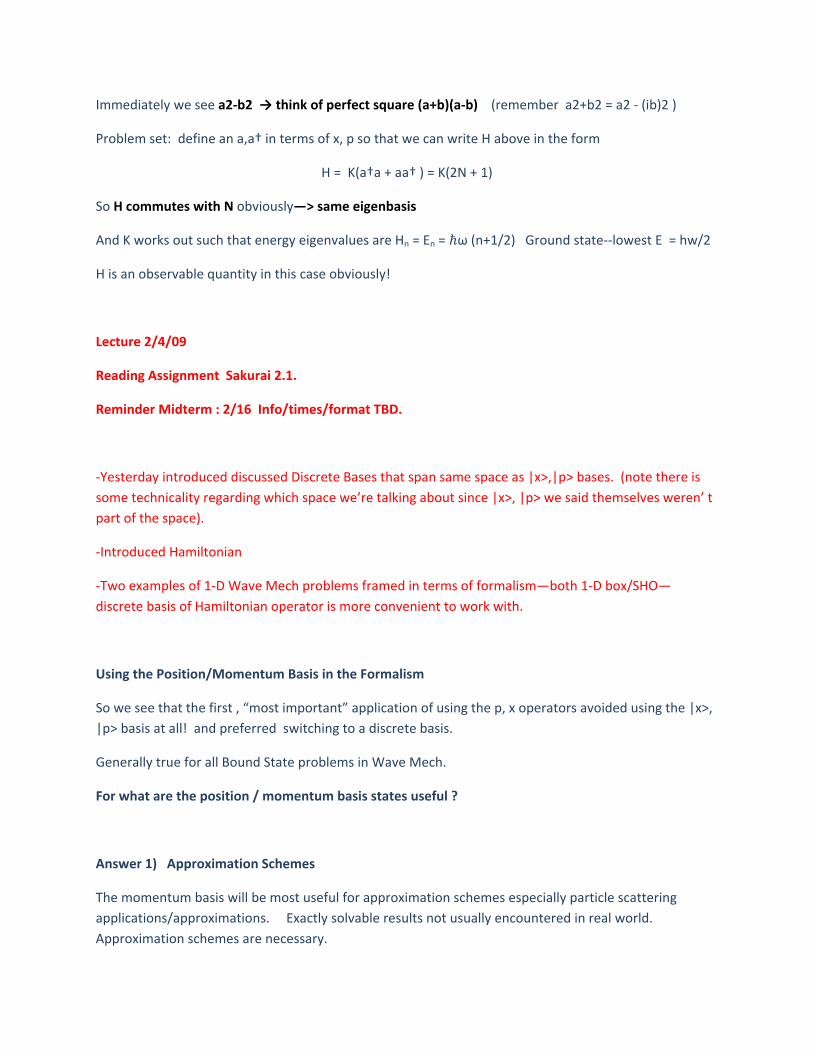
Immediately we see a2‐b2  → think of perfect square (a+b)(a‐b)    (remember  a2+b2 = a2 ‐ (ib)2 ) 

Problem set:  define an a,a† in terms of x, p so that we can write H above in the form 

H =  K(a†a + aa† ) = K(2N + 1) 

So H commutes with N obviously—> same eigenbasis 

And K works out such that energy eigenvalues are Hn = En =  ω (n+1/2)   Ground state‐‐lowest E  = hw/2 

H is an observable quantity in this case obviously! 

 

Lecture 2/4/09 

Reading Assignment  Sakurai 2.1. 

Reminder Midterm : 2/16  Info/times/format TBD. 

 

‐Yesterday introduced discussed Discrete Bases that span same space as |x>,|p> bases.  (note there is 

some technicality regarding which space we’re talking about since |x>, |p> we said themselves weren’ t 

part of the space). 

‐Introduced Hamiltonian   

‐Two examples of 1‐D Wave Mech problems framed in terms of formalism—both 1‐D box/SHO—  

discrete basis of Hamiltonian operator is more convenient to work with.    

 

Using the Position/Momentum Basis in the Formalism 

So we see that the first , “most important” application of using the p, x operators avoided using the |x>, 

|p> basis at all!  and preferred  switching to a discrete basis. 

Generally true for all Bound State problems in Wave Mech. 

For what are the position / momentum basis states useful ? 

 

Answer 1)   Approximation Schemes 

The momentum basis will be most useful for approximation schemes especially particle scattering 

applications/approximations.     Exactly solvable results not usually encountered in real world.  

Approximation schemes are necessary. 

Notice two things about the Hamiltonian:   H = p2/2m + V(x)  = T + V(x) 

1) Obviously with V(x) = 0  The momentum  basis is also the basis of the Hamiltonian. 

2) We should usually be able to approximate potentials V(x)  as some sort  of series sum    

Most obvious such expansion     V(x) = V1(x) + V2 (x)+…  like Taylor expansion where other later terms 

are relatively smaller and smaller, so we can drop them.  

 

Separable Potentials 

But we can also do expansions of a kind that is more convenient towards using a particular set of basis 

states: 

Following the idea of making a general operator out of ket‐bra outer products (e.g. we said in it’s own 

eigenbasis an operator A has the form ∑ an |an><an|) it can be useful  to  approximate using arbitrary 

potentials in the form 

V = |g>λgf <f| 

Where ,g,f can be some state, which can of course be written as linear combinations of basis states, 

possibly momentum kets |p> or position kets |x>  and λ is some number. 

Potentials are called separable if they can be written as a combination of such terms (e.g. most 

commonly a discrete sum )  

Vsep = ∑kn |k>λ kn<n| 

I think that word is used because it acts on each combination of basis  states  ”separately.” 

A convenient choice for these could be the momentum basis states 

∫ dpdp’   |p>λpp<p’| 

Why ?  Because then the entire Hamiltonian including the p2/2m operator (sometimes called T)  is 

entirely composed of operators which act directly on |p> basis kets !!! 

YESTERDAY NUCLEAR SEMINAR:  EXACTLY ONE EXAMPLE!!! 

DIGRESSION:  Why momentum kets instead of position? 

Greater question:  Perfect symmetry between p, x?       PSET:  The Position Operator in the |p> Basis—  

also fulfills derivative relation 

<p|x|α>    d/dp (<p|α>) = dϕ(p)/dp     

So everything looks very symmetric. 

Answer: no generally because of free Hamiltonian “preference” for p operator.  p is likely the usually the 

preferred basis (in lieu of exact Hamiltonian basis). 

Actually for separable potentials, it is actually usually angular momentum basis states. 

end DIGRESSION 

 

Perturbation Theory:   

More generally there is perturbation theory which we will not discuss this quarter.   But we discussed it 

during the Wave Mech review (please go back and take a look)—its generalization in the bra/ket 

formalism should not be hard to imagine.    

For high energy scattering problems,  it is most convenient to treat the “base Hamiltonian” as  

H0 =  p2/2m  = T 

and because by assumption the T = KE is so high, treat the entire potential V(x) as a perturbation.  Thus 

again the base states you want to start w/ for H0 are obviously the |p> states. 

The main difference between Perturbation Theory though is that PT is a full expansion of the STATES of 

the full Hamiltonian, in terms of the states of the base H, not just an approximate expansion of the 

potential. 

 

Answer 2)  “Artificial” Construction of States 

Another reason |p>, |x>  basis useful is it’s easy to construct arbitrary states using them—through the 

wave functions themselves.    Sometimes we may not know or care what the Hamiltonian is, but we 

have a better idea how to describe the state in terms of the |x> or |p> states.    

Examples:  

‐Suppose we know a particle is localized to some area 

‐ Suppose we know its momentum 

This is especially useful for the question of initial state.   

Remember question:  What is the state of the particle before it hits the SG device?    Spin states may 

not be determined, but there is also a momentum/position state for the atom:  this we do have some 

idea how it should look. 

A) it has some fixed momentum.   (this has to be tuned right to “see” the splitting due to spin)  

within some uncertainty range 

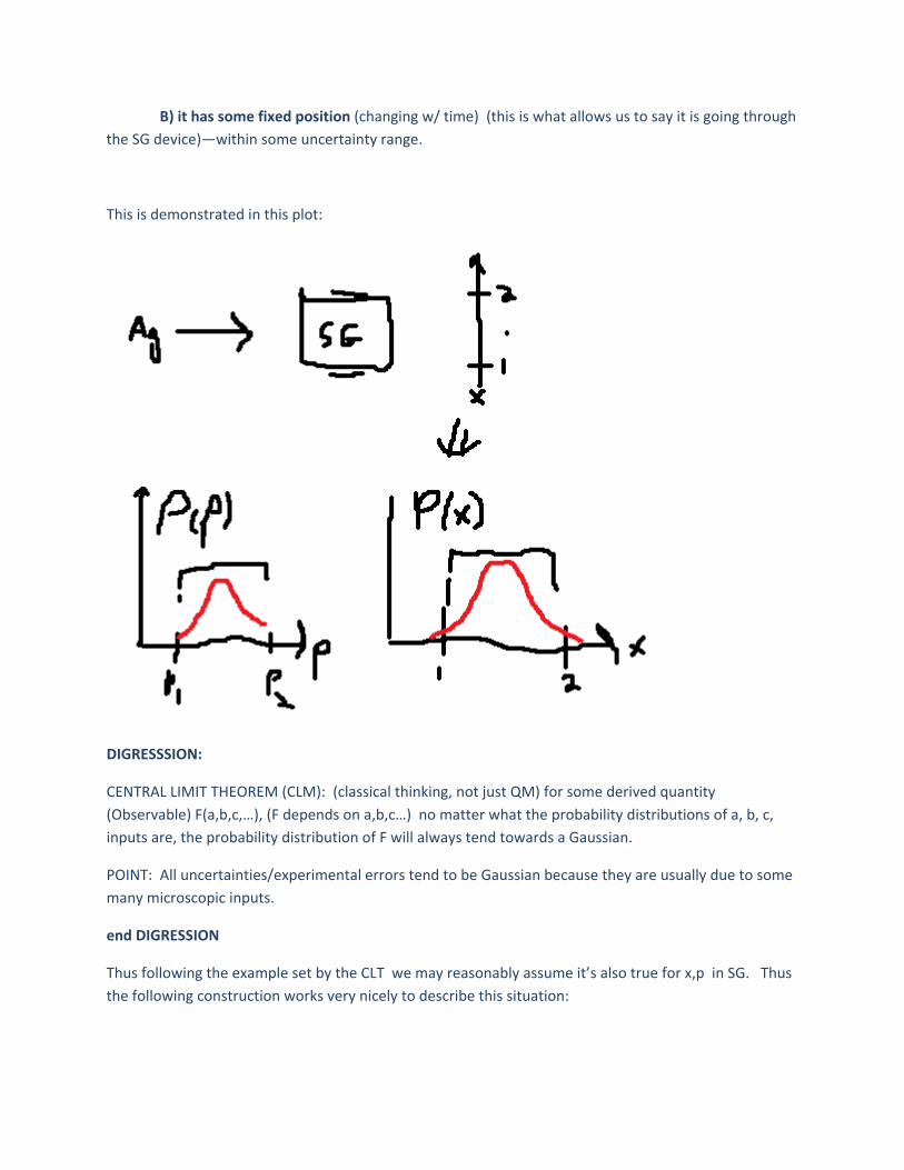
B) it has some fixed position (changing w/ time)  (this is what allows us to say it is going through 

the SG device)—within some uncertainty range. 

 

This is demonstrated in this plot: 

 

DIGRESSSION: 

CENTRAL LIMIT THEOREM (CLM):  (classical thinking, not just QM) for some derived quantity 

(Observable) F(a,b,c,…), (F depends on a,b,c…)  no matter what the probability distributions of a, b, c, 

inputs are, the probability distribution of F will always tend towards a Gaussian. 

POINT:  All uncertainties/experimental errors tend to be Gaussian because they are usually due to some 

many microscopic inputs. 

end DIGRESSION  

Thus following the example set by the CLT  we may reasonably assume it’s also true for x,p  in SG.   Thus 

the following construction works very nicely to describe this situation: 

 

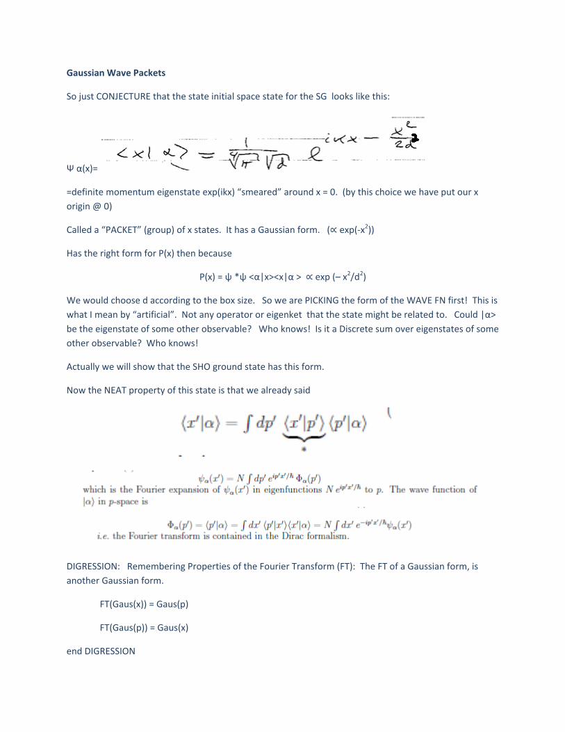
Gaussian Wave Packets 

So just CONJECTURE that the state initial space state for the SG  looks like this: 

Ψ α(x)=   

=definite momentum eigenstate exp(ikx) “smeared” around x = 0.  (by this choice we have put our x 

origin @ 0)    

Called a “PACKET” (group) of x states.  It has a Gaussian form.   (  exp(‐x2)) 

Has the right form for P(x) then because  

P(x) = ψ *ψ <α|x><x|α >    exp (– x2/d2) 

We would choose d according to the box size.   So we are PICKING the form of the WAVE FN first!  This is 

what I mean by “artificial”.  Not any operator or eigenket  that the state might be related to.   Could |α> 

be the eigenstate of some other observable?   Who knows!  Is it a Discrete sum over eigenstates of some 

other observable?  Who knows!     

Actually we will show that the SHO ground state has this form. 

Now the NEAT property of this state is that we already said   

 

 

DIGRESSION:   Remembering Properties of the Fourier Transform (FT):  The FT of a Gaussian form, is 

another Gaussian form.  

FT(Gaus(x)) = Gaus(p)    

FT(Gaus(p)) = Gaus(x) 

end DIGRESSION 

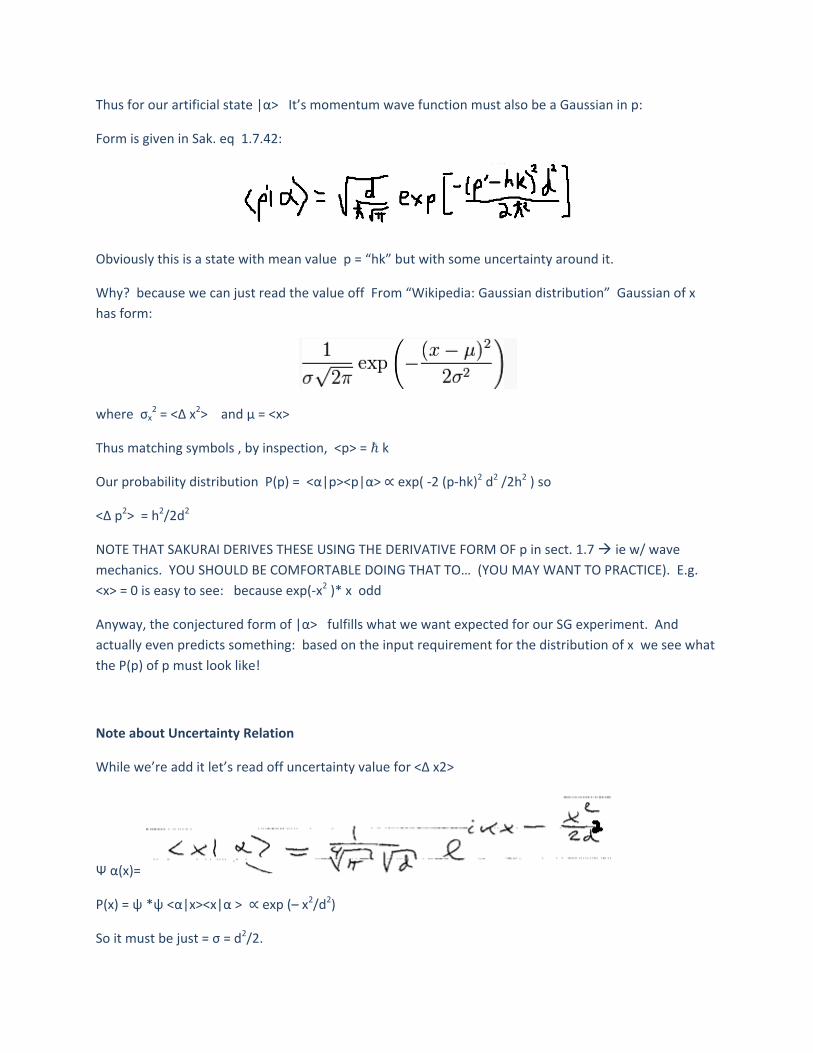
Thus for our artificial state |α>   It’s momentum wave function must also be a Gaussian in p: 

Form is given in Sak. eq  1.7.42: 

 

Obviously this is a state with mean value  p = “hk” but with some uncertainty around it. 

Why?  because we can just read the value off  From “Wikipedia: Gaussian distribution”  Gaussian of x 

has form: 

 

where  σx2 = <Δ x2>    and μ = <x> 

Thus matching symbols , by inspection,  <p> =   k 

Our probability distribution  P(p) =  <α|p><p|α>   exp( ‐2 (p‐hk)2 d2 /2h2 ) so  

<Δ p2>  = h2/2d2 

NOTE THAT SAKURAI DERIVES THESE USING THE DERIVATIVE FORM OF p in sect. 1.7  ie w/ wave 

mechanics.  YOU SHOULD BE COMFORTABLE DOING THAT TO…  (YOU MAY WANT TO PRACTICE).  E.g.  

<x> = 0 is easy to see:   because exp(‐x2 )* x  odd 

Anyway, the conjectured form of |α>   fulfills what we want expected for our SG experiment.  And 

actually even predicts something:  based on the input requirement for the distribution of x  we see what 

the P(p) of p must look like! 

 

Note about Uncertainty Relation 

While we’re add it let’s read off uncertainty value for <Δ x2>   

Ψ α(x)=   

P(x) = ψ *ψ <α|x><x|α >    exp (– x2/d2) 

So it must be just = σ = d2/2.