Sphere systems in 3-manifolds and arc graphs

by

Francesca Iezzi

Thesis

Submitted to the University of Warwick

for the degree of

Doctor of Philosophy

Mathematics

March 2016

Contents

Acknowledgments iii

Declarations vi

Abstract vii

Introduction 1

Background . . . . . . . . . . . . . . . . . . . . . . . . . . . . . . . . . . . 1

Main results . . . . . . . . . . . . . . . . . . . . . . . . . . . . . . . . . . . 6

Outline of the Thesis . . . . . . . . . . . . . . . . . . . . . . . . . . . . . . 10

Chapter 1 Sphere graphs of manifolds with holes 1

1.1 Some questions . . . . . . . . . . . . . . . . . . . . . . . . . . . . . . 4

Chapter 2 Standard form for sphere systems 5

2.1 Intersection of spheres, Minimal and Standard form . . . . . . . . . 6

2.1.1 Spheres, partitions and intersections . . . . . . . . . . . . . . 7

2.1.2 Minimal and standard form . . . . . . . . . . . . . . . . . . . 15

2.2 Dual square complex . . . . . . . . . . . . . . . . . . . . . . . . . . . 17

2.3 Inverse construction . . . . . . . . . . . . . . . . . . . . . . . . . . . 24

2.4 The core of two trees . . . . . . . . . . . . . . . . . . . . . . . . . . . 37

2.5 Consequences . . . . . . . . . . . . . . . . . . . . . . . . . . . . . . . 48

2.6 The case where the two systems contain spheres in common . . . . . 56

2.6.1 Constructing a dual square complex in the case where the two

sphere systems contain spheres in common . . . . . . . . . . 56

2.6.2 Inverse construction in the general case . . . . . . . . . . . . 58

2.6.3 The core of two trees containing edges in common . . . . . . 60

2.6.4 Consequences in the case of sphere systems with spheres in

common . . . . . . . . . . . . . . . . . . . . . . . . . . . . . . 63

i

2.7 Future directions . . . . . . . . . . . . . . . . . . . . . . . . . . . . . 64

Chapter 3 Sphere and arc graphs 66

3.1 Injections of arc graphs into sphere graphs . . . . . . . . . . . . . . . 67

3.2 Proof of Theorem 3.1.2 . . . . . . . . . . . . . . . . . . . . . . . . . . 70

3.2.1 Defining the retraction: first naive idea and main problems

arising . . . . . . . . . . . . . . . . . . . . . . . . . . . . . . . 70

3.2.2 Efficient position for spheres and surfaces . . . . . . . . . . . 71

3.2.3 Is the retraction well defined? . . . . . . . . . . . . . . . . . . 76

3.2.4 Proof of Theorem 3.1.2 . . . . . . . . . . . . . . . . . . . . . 81

3.3 Some consequences about the diameter of sphere graphs . . . . . . . 83

3.4 Questions . . . . . . . . . . . . . . . . . . . . . . . . . . . . . . . . . 84

Appendix A Maps between graphs and surfaces 86

Appendix B A further proof of Lemma 2.2.3 89

Bibliography 96

ii

Acknowledgments

It seems like it was only yesterday that I left my country, my family and friends, to

come to a different place, speaking a language which I was not very familiar with.

On the one hand I remember being excited, but on the other hand very sad and

scared. Now that this “cycle of my life”has almost come to an end, I look back and

I acknowledge that these four years have been a very important part of my life, and

that, throughout this period I grew a lot both from an educational point of view

and from a personal point of view.

I would not be at this stage without the help of a lot of people, who deserve

all of my gratitude.

First of all, I am really grateful to my advisor, Brian Bowditch, for accepting

me as his student, and above all for his kind and patient guidance and advice. I

thank him for teaching me a lot and challenging me often. I have learnt a lot from

his teaching and from his impressive mathematical talent.

I am very thankful to Karen Vogtmann and Arnaud Hilion for agreeing to

examine my work, for many useful comments on how to improve my thesis, and for

making my thesis defence an instructive and enjoyable experience.

I would like to thank Saul Schleimer for very useful and stimulating mathe-

matical conversations, and for pointing out a mistake in an early draft of my thesis.

I thank Sebastian Hensel for many stimulating discussions.

I am thankful to all who have been members of the Geometry and Topology

group at Warwick during these four years for many interesting discussions and for

the support they have given me. A special mention goes to Beatrice and Federica

for their support in the pre-submission and post-submission period.

iii

I am extremely grateful to all the people who, over these four years and in

particular in these last few months, have generously spent part of their time to help

me overcome some difficulties in using LaTex and inkscape.

I thank my fellow graduate students and young postdocs at Warwick, I thank

in particular those with whom I had the possibility to share the joys, but also the

difficulties and challenges a graduate student constantly faces. Without them, I

would have felt much more lonely over the last four years.

I am grateful to all the staff working in the Maths Department at Warwick

University, for their efficiency, and for making the department a wonderful work

environment.

I am very thankful to The Engineering and Physical Sciences Research Coun-

cil for founding my doctoral studies.

Two years ago I spent seven fruitful and unforgetable months in Tokyo, vis-

iting the Tokyo Institute of Technology. This experience was very fruitful workwise

and, on the other hand gave me the opportunity to challenge myself, and to experi-

ence a different culture. I could never be thankful enough to my advisor, for giving

me the opportunity to have this experience, and to Prof Kojima and his lab at

the Tokyo Institute of Technology, for welcoming me and helping me in overcoming

many of the practical issues.

I would like to express my gratitude to Fr Harry and the members of the

Catholic Society at the University of Warwick. My life at Warwick would have lacked

something if I had not had the opportunity to be part of this Society. Through the

society I met some of my best friends. Moreover, attending the society activities

and sharing my experiences with other people helped me a lot in looking at things

from a different perspective and in finding the right balance in different aspects of

my life.

These years would have been much sadder and lonelier without the help and

the support of many friends. I apologise for not mentioning them by name, but

they are many, and I would risk forgetting to mention somebody. I thank many

good friends I have met while studying in Pisa, whom, despite the distance, have

iv

continued to be people I could count on. I thank friends whom I have met during

my studies at Warwick, with whom I have shared happy moments, and to whom

I have turned during the most challenging periods to seek support. Some of them

have spent a long period here, some of them have spent too short a period here,

unfortunately, but all of them have been and are an important part of my life.

Finally, I could never thank my family enough. It is thanks to them that

I developed the curious personality which led me to undertake this Ph.D. I’d like

in particular to thank my parents for continuously supporting me during these last

four years, and for helping me to keep my feet on the ground. A special mention

goes to my mother for her practical help in some crucial moments over the last years

as well as for her neverending support.

v

Declarations

I declare that the material in this thesis is, to the best of my knowledge, my own

except where otherwise indicated or cited in the text, or else where the material is

widely known. This material has not been submitted for any other degree, and only

the material from Chapter 3 has been submitted for peer-reviewed pubblication.

All figures were created by the author using inkscape.

vi

Abstract

We present in this thesis some results about sphere graphs of 3-manifolds.If we denote as Mg the connected sum of g copies of S2×S1, the sphere graph

of Mg, denoted as S(Mg), is the graph whose vertices are isotopy classes of essentialspheres in Mg, where two vertices are adjacent if the spheres they represent can berealised disjointly. Sphere graphs have turned out to be an important tool in thestudy of outer automorphisms groups of free groups.

The thesis is mainly focused on two projects.

As a first project, we develop a tool in the study of sphere graphs, viaanalysing the intersections of two collections of spheres in the 3-manifold Mg.

Elaborating on Hatcher’s work and on his definition of normal form forspheres ([15]), we define a standard form for two embedded sphere systems (i.ecollections of disjoint spheres) in Mg.

We show that such a standard form exists for any couple of maximal spheresystems in Mg, and is unique up to homeomorphisms of Mg inducing the identityon the fundamental group.

Our proof uses combinatorial and topological methods. We basically showthat most of the information about two embedded maximal sphere systems in Mg

is contained in a 2-dimensional CW complex, which we call the square complexassociated to the two sphere systems.

The second project concerns the connections between arc graphs of surfacesand sphere graphs of 3-manifolds.

If S is a compact orientable surface whose fundamental group is the freegroup Fg, then there is a natural injective map i from the arc graph of the surface Sto the sphere graph of the 3-manifold Mg. It has been proved ([12]) that this mapis an isometric embedding.

We prove, using topological methods, that the map i admits a coarsely de-fined Lipschitz left inverse.

vii

Introduction

The main objects of study during my Ph.D have been sphere graphs of 3-manifolds

and arc graphs of surfaces. I focused in particular on the connection between these

two spaces.

Both objects play an important role in Geometric Group Theory, since they

act as important tools in the study of some of the central topics in the area: Mapping

Class Groups of surfaces and Outer Automorphisms of Free Groups.

Background

Given a compact orientable surface S, the Mapping Class Group of S (we will

denote it as Mod(S)) is the group of isotopy classes of orientation preserving self-

homeomorphisms of the surface. The group of all isotopy classes of self-homeomorphisms

of S (both orientation preserving and orientation reversing) is often called the ex-

tended Mapping Class Group and denoted as Mod±(S). Note that Mod(S) is a

subgroup of Mod±(S) of index two.

These objects have been among the most important objects of study in Geo-

metric topology over the last sixty years. A very important theorem states that the

Mapping Class group of a closed orientable surface S is generated by Dehn twists

around simple closed curves in S; a proof of this result can be found in [28]. Lick-

orish proved ([29]) that a finite number of Dehn twists is sufficient to generate the

Mapping Class Group of a closed surface. A lot of progress has been made and

inspired by Thurston.

Key tools in the study of surface Mapping class groups are Teichmuller spaces

and curve complex, which I define below.

The Teichmuller space of a surface S is the space of marked hyperbolic met-

rics on S up to isotopy. The group Mod(S) acts on the Teichmuller space of S

properly discontinuously. I refer to [8] for some more detailed background about

surface Mapping Class Groups and Teichmuller spaces.

1

The curve complex of a surface S (usually denoted as C(S)) is the simplicial

complex whose vertices are isotopy classes of simple closed curves on the surface S,

where k + 1 curves span a k-simplex if they can be realised disjointly.

This complex was first introduced by Harvey ([14]) as a combinatorial tool

for the study of Teichmuller spaces. Ivanov ([23]) proved that, if S is a surface of

genus at least two, then the group of simplicial automorphisms of the complex C(S)

is the group Mod±(S).

Great progress in the study of the geometry of the curve complex has been

made by Masur and Minsky ([32] and [33]). In particular they prove ([32]) that the

curve complex is hyperbolic. Shorter proof of the hyperbolicity of the curve complex

using combinatorial methods can be found in [3] and [19].

The arc complex of a surface S with boundary is an analogue of the curve

complex. Vertices in this complex are isotopy classes of embedded essential arcs

in S; again k + 1 arcs span a k-simplex if they can be realised disjointly. The arc

complex has also been proven to be hyperbolic. Independent proofs can be found

in [20], [31] and [19]. In particular, in [19] the authors show that the hyperbolicity

constant does not depend on the surface.

Automorphism groups of free groups have been an object of study in combi-

natorial group theory since the first decades of last century, and has interacted with

the study of linear groups GLn(Z), and with the study of surface Mapping Class

Groups. I will explain the connections below.

On the one hand there is a natural map Aut(Fn) → GLn(Z). Since inner

automorphisms of Fn are contained in the kernel of this map, this map factors

through the group of outer automorphisms, denoted as Out(Fn).

On the other hand, if Sg,b is the surface of genus g with b > 0 punctures, then

the fundamental group of S is the free group Fn, where n = 2g + b − 1. Therefore

there is a natural map from the extended Mapping Class Group of S to the group

Out(Fn), mapping a self-homeomorphism of S to its action on π1(S). Note that,

since the choice of a base point is arbitrary, this map may not be well defined as a

map to the group Aut(Fn). This map is injective but is not surjective. The image of

this map is the subgroup of Out(Fn) fixing the set of curves surrounding individual

punctures, up to conjugacy (see [8] Theorem 8.8).

Both examples mentioned above show that it is natural to study the group

Out(Fn) i. e. the quotient of the group Aut(Fn) by inner homeomorphisms.

In the very special case where n = 2, it is known that the group Out(F2) is

isomorphic to the group GL2(Z) and to the group Mod±(S1,1).

2

Great contributions to the study of the groups Aut(Fn) and Out(Fn) have

been made by Nielsen and Whithehead in the first half of the twentieth century.

In particular, in the 20s Nielsen found a finite set of generators for the group of

automorphisms of a free group, known as Nielsen basis. A consequence of Nielsen

result is that the map Out(Fn)→ GLn(Z) given by abelianisation of Fn is surjective.

In the 70-80s, due to progress made by Thurston and Gromov, people started

using geometric and topological methods to study the groups Out(Fn). The idea

is to deduce some algebraic properties of the group by analysing the action of the

group on a metric space. Methods used to study surfaces Mapping Class Groups

inspired new ideas in the study of the groups Out(Fn).

The first candidate to play the role of the surface in the study of the Mapping

Class Group would be a graph with fundamental group Fn.

In [7] Culler and Vogtmann introduced a space CVn which mimics the role

of Teichmuller space in the study of mapping class groups. The space CVn has been

named the Culler-Vogtmann space or the Outer space of rank n. Elements of CVn

are marked metric graphs (i.e. graphs endowed with a metric and with a homotopy

equivalence to the bouquet of n circles). The group Fn acts on CVn with finite point

stabilisers. In [7] the authors prove that this space is contractible. They also define

a spine Kn on which the space CVn retracts.

There is another topological object which can play the same role as a marked

graph. This space is the connected sum of n copies of S2 × S1. We will denote this

3-manifold by Mn. The fundamental group of the manifold Mn is the free group

Fn. There is a map Mod(Mn) → Out(Fn), mapping a self-homeomorphism of the

manifold to its action on the fundamental group.

This map is surjective: it can be checked that each element of a Nielsen basis

for Aut(Fn) can be represented as a self-homeomorphism of the manifold Mn (a

proof can be found in [27] p. 81). It has been proven by Laudenback ([27] p. 80)

that the kernel of this map is generated by a finite number of sphere twists; where,

if σ is an essential sphere in Mn, a sphere twist around σ is a self-homeomorphism of

Mn supported in the neighborhood σ× [0, 1] rotating of 360 degrees around an axis

of the sphere σ. More precisely, choose a non trivial loop α based at the identity in

the group of rotations SO(3); note that, since the fundamental group of SO(3) is

Z2 two such loops are homotopic. Now let σ be an embedded sphere in Mn and let

Nσ = σ× [0, 1] be a tubular neighbourhood of σ; we define the twist Tσ around the

sphere σ in the following way:

If x /∈ N then Tσ(x) = x

If x = (y, t) ∈ N = σ × [0, 1] then Tσ(x) = (α(t)(y), t).

3

A sphere twist Tσ is defined by the isotopy class of σ. Since the fundamental

group of SO(3) is Z2, a sphere twist has order two. Intuitively a sphere twist is a

tri-dimensional version of a Dehn twist around a curve.

The idea of using the manifold Mn as a tool in the study of Out(Fn) goes

back to Whitehead ([36]), who used Mn to find an algorithm to decide whether a

map from Fn to Fn is an automorphism. I refer to [35] for an outline of Whitehead’s

methods.

Building on Whitehead’s ideas, in [15] Hatcher introduces the sphere complex

of the manifold Mn, denoted as S(Mn). The vertices of this complex are isotopy

classes of embedded essential spheres in Mn, where by essential I mean that they

do not bound a ball. A k-simplex in this complex corresponds to a system of

k + 1 spheres, i. e. a collection of k + 1 disjoint non pairwise isotopic spheres.

This complex is well defined, since by a theorem by Laudenbach ([26] Theoreme

I) homotopic spheres in Mn are isotopic; Euler characteristic arguments show that

the dimension of S(Mn) is 3n− 4. Again in [15], the author proves that the sphere

complex is contractible.

Since every sphere twist acts trivially on the sphere complex, the action of

the Mapping Class Group of Mn on the complex S(Mn) factors through an action

of Out(Fn) on S(Mn). This group action makes the sphere complex an interesting

tool in the study of the group Out(Fn).

Using spheres in 3-manifolds one can find an equivalent way to define Culler-

Vogtmann space, in fact, elements of CVn can be defined as weighted sphere systems

in the manifold Mn; this different approach to the definition of the Outer Space is

described in the appendix of [15]. In particular, a subcomplex of the first baricentric

subdivision of S(Mn) is isomorphic the spine Kn of the space CVn. The vertices of

this subcomplex are sphere systems in Mn with simply connected complementary

components. The groupOut(Fn) acts properly and cocompactly on this subcomplex,

therefore this subcomplex is quasi-isometric to Out(Fn).

In [16] Hatcher and Vogtmann use the sphere complex to prove the existence

of upper bounds for isoperimetric functions of automorphism groups of free groups.

In [17] the same authors use sphere systems in the manifold Mn to build a

topological model for the free factor complex of a free group (defined as the geometric

realization of the partially ordered set of proper free factors of a free group). In the

same article the authors prove that the complex of free factors of the group Fn is

homotopy equivalent to a wedge of spheres of dimension n− 2.

The sphere complex S(Mn) also admits a purely algebraic definition, it can

be defined as the free splitting complex of the group Fn. The vertices of this complex

4

are free splittings of the group Fn, two vertices are adjacent if the corresponding

splittings admit a common refinement. I refer to [13] for a more precise definition

of the free splitting complex.

A proof of the fact that the 1-skeleton of the sphere complex (which we

will denote as the sphere graph) is isomorphic to the 1-skeleton of the free splitting

complex can be found in [1]; this isomorphism is equivariant under the action of

Out(Fn). In the same article the authors prove an Out(Fn) equivalent of Ivanov’s

theorem, i.e. Out(Fn) is the group of simplicial automorphisms of the free splitting

graph if n ≥ 3. Thanks to this result the sphere graph of Mn can be seen as an

analogue of the curve complex in the study of Out(Fn).

As for the coarse geometry, it has been recently proven ([13]) that the free

splitting complex is hyperbolic. A shorter proof of this result, using the topological

model (i. e. the sphere complex) can be found in [20]. This result establishes a

further analogy between the curve complex of a surface and the sphere complex of

a 3-manifold.

As a note, also the free factor complex has been recently proved to be hy-

perbolic ([2]). Moreover, in [24] the authors use hyperbolicity of the free splitting

complex to deduce hyperbolicity of the free factor complex.

One of the key tools in the study of the properties of the sphere complex is

the existence of a normal form for spheres with respect to a maximal sphere system

Σ. This normal form has been defined by Hatcher in [15] and is a key ingredient in

the proof of contractibility of the sphere complex, as well as in the proofs of many

results in [16], [17] and [20]. Intuitively a sphere σ is in normal form with respect to

a sphere system Σ if σ intersects the system Σ in a minimal number of circles. This

definition can be extended to a finite collection of spheres. Hatcher proves ([15]

Theorem 1.1) that each finite collection of spheres can be represented in normal

form with respect to any maximal sphere system Σ. He also proved ([15] Theorem

1.2) that two isotopic collections of spheres both in normal form with respect to a

system Σ are equivalent, i. e. there is a homotopy between these two collections of

spheres which restricts to an isotopy on the intersection with the system Σ.

Hatcher’s definition of normal form inspired the work described in Chapter

2. Namely, building on Hatcher’s ideas, we define a standard form for two embedded

sphere systems in Mn; this standard form is a refinement of Hatcher’s normal form.

We show that a standard form always exists (Theorem 2.5.4) and is essentially

unique (Theorem 2.5.6). All the proofs are independent on Hatcher’s work. We use

combinatorial and topological methods. Similar methods have been used in [22] to

estimate distances in Outer space. Similar methods have also been used in [9] to

5

give a proof of a criterion determining when a conjugacy class in π2(Mg) can be

represented by an embedded sphere. However, these articles came to my attention

after writing Chapter 2.

The work described in Chapter 3 concerns the connection between arc graphs

of a surface and sphere graphs of a 3-manifold. Namely, if S is any surface whose

fundamental group is the free group Fn of rank n, then there is a natural injective

map i from the arc graph (i.e. the 1-skeleton of the arc complex) of the surface S to

the sphere graph of the manifold Mn. We will define this map in the next section.

We will show in Chapter 3 that the map i admits a Lipschitz coarse left inverse.

The existence of the map i has been used in [11] and [12] to prove that

Mod(Sg,1) is an undistorted subgroup of Out(F2g) (i. e. the map Mod(Sg,1) →Out(F2g) mapping a homeomorphism of S to its action on the fundamental group

is a quasi-isometric embedding).

The map i has been proven to be an isometric embedding in [12], in the

particular case where n is even and S is a surface with one boundary component.

The authors also define a retraction from the sphere graph of M2g to the arc graph

of Sg,1. This map is not canonical though, since it depends on a choice of a collection

of arcs on the surface S.

The aim of Chapter 3 is to prove Theorem 3.1.2, stating that for any n

and any surface having Fn as fundamental group there exists a canonical Lipschitz

coarse left inverse for the map i. An immediate consequence is that the map i is a

quasi-isometric embedding.

I will give a more detailed outline of the main results in the next section

Main results

This thesis contains mainly two related projects.

The first project concerns work described in Chapter 2. As mentioned, we

define a refinement of Hatcher’s normal form. Before stating the main results I recall

some basic definitions and introduce some notation and terminology.

For g ≥ 2 we denote as Mg the connected sum of g copies of S2 × S1, and

we denote as Mg the universal cover of Mg. Note that Mg can be constructed by

taking two copies of the handlebody of genus g and gluing their boundaries together

along a map which is isotopic to the identity.

An essential sphere in Mg is an embedded 2-sphere which does not bound a

ball. Recall that by work of Laudenbach two homotopic spheres in Mg are isotopic.

6

Given two embedded spheres σ1 and σ2 in Mg we always suppose they in-

tersect transversally and therefore their intersection consists of a finite collection of

circles. We say that σ1 and σ2 intersect minimally if there do not exist spheres σ′1and σ′2 homotopic to σ1 and σ2 respectively, and such that σ′1 ∩ σ′2 contains fewer

circles than σ1 ∩ σ2.

A sphere system is a collection of disjoint pairwise non isotopic essential

spheres in Mg.

A sphere system Σ is said to be maximal if it is maximal with respect to

inclusion, i. e. any sphere disjoint from Σ is isotopic to a sphere contained in Σ.

Note that Σ is maximal if and only if all of its complementary components in Mg

are 3-holed 3-spheres (where by a 3-holed 3-sphere I mean the manifold obtained by

removing from the 3-sphere S3 the interior of three disjoint embedded balls).

Given two maximal sphere systems Σ1 and Σ2 in Mg we say that they have

no spheres in common if there is no sphere in the system Σ1 homotopic to a sphere

in the system Σ2.

We are ready to give the following:

Definition. Let Σ1 and Σ2 be two maximal sphere systems in Mg. We say that they

are in minimal form if each sphere in Σ1 intersects each sphere in Σ2 minimally.

We say that Σ1 and Σ2 are in standard form if all the complementary components

of Σ1 ∪ Σ2 in Mg are handlebodies.

We prove the following:

Theorem. (I) Any two maximal sphere systems Σ1 and Σ2 in Mn can be homotoped

to be in standard form with respect to each other.

Theorem. (II) Standard form is essentially unique. Namely: given two pairs of

sphere systems, (Σ1,Σ2) and (Σ′1,Σ′2), both in standard form, and so that Σi is

homotopic to Σ′i for i = 1, 2; then there exists a self homeomorphism of Mn mapping

(Σ1,Σ2) to (Σ′1,Σ′2). This homeomorphism acts trivially on the fundamental group

of Mn.

To prove these results we use combinatorial and topological methods. We

show that a standard form for two sphere systems depends only on the isomorphism

class of a particular CAT(0) square complex, which we call the dual square complex.

We show that this complex can be constructed abstractly just by looking at two

actions of the group Fg on trivalent trees.

The results stated above are proved in full detail in the case where the two

sphere systems have no spheres in common. However, the same techniques can be

7

used to prove the same results in the general case. I give an outline on how to deal

with general case in Section 2.6.

In the next section we give a brief outline of the proof of Theorem (I) and

Theorem(II).

The work described in Chapter 3 concerns the connection between sphere

graphs of 3-manifolds and arc graphs of surfaces.

I have quickly defined in the previous section the arc complex of a surface and

the sphere complex of a 3-manifold. These are both simplicial complexes of finite

dimension in general bigger than one. Note anyway that, since the work described

in Chapter 3 concerns the coarse geometry of these complexes, we will work with the

1-skeleta of both complexes, knowing that a finite dimensional simplicial complex is

quasi-isometric to its 1-skeleton.

We first recall some basic definitions.

If S is a surface with non empty boundary, an essential arc on S is a properly

embedded non boundary parallel arc on S.

Definition. Given a compact orientable surface S with non empty boundary the arc

graph of the surface S, denoted as A(S), is the graph whose vertices are homotopy

classes (rel. boundary) of essential arcs on S. Two vertices are adjacent if the

corresponding arcs can be realised disjointly.

Recall that we denote as Mg the connected sum of g copies of S2 × S1, and

by Vg the handlebody of genus g.

Definition. Given a 3-manifold Mg the sphere graph of Mg, denoted as S(Mg),

is the graph whose vertices are homotopy classes of essential spheres in Mg. Two

vertices are adjacent if the corresponding spheres can be realised disjointly.

If S is any surface whose fundamental group is the free group Fg. then there

is a natural map i : A(S)→ S(Mg).

To understand how the map i is defined, note first that Mg can be con-

structed abstractly as the double of the handlebody Vg of genus g, and that Vg is

homeomorphic to the trivial interval bundle over the surface S. In light of what we

just said, we can identify the surface S to a surface embedded in Mg; denote the em-

bedding by ϕ and note that ϕ induces an isomorphism on the level of fundamental

groups.

Consider now an essential properly embedded arc a in the surface S; if we

take the interval bundle over the arc a we obtain a disc in Vg, the double of this disc

is an essential sphere σ in the manifold Mg. Set i(a) = σ.

8

The map i is well defined on the arc graph, 1-Lipschitz (since disjoint arcs

are mapped to disjoint spheres), and injective (as shown in Lemma 3.1.1).

The aim of Chapter 3 is to construct a coarse left inverse p for the map i.

There is a naive way to try to construct the map p, i.e. given a sphere σ

(transverse to ϕ(S)), consider the intersection σ ∩ ϕ(S) and define p(σ) as any arc

in (the preimage through ϕ of) this intersection; we call the set ϕ−1(σ ∩ ϕ(S)) the

arc pattern induced by ϕ and σ.

The map p defined above, however, may not be well defined, since modifying

the map ϕ and the sphere σ by homotopy may change the homotopy class of the

collection of arcs ϕ−1(σ ∩ ϕ(S)).

To solve this problem, we first define an efficient position for a map ϕ : S →Mg and a sphere σ (Section 3.2.2). Then we show (Theorem 3.2.12) that, provided

the map ϕ is efficient with respect to the sphere σ, the arc pattern induced by ϕ and

σ is determined, up to bounded distance in the arc graph of S, by the homotopy

class of ϕ and σ.

This allows us to prove the following:

Theorem. (III) There is a canonical coarsely defined Lipschitz coarse retraction

p : S(Mg) → A(S). The map p is defined up to distance seven and the Lipschitz

constant is at most 15. Moreover, p is well defined if restricted to the subgraph

i(A(S)) and coincides in this case with the inverse map i−1.

An immediate consequence of Theorem 3.1.2 is the following:

Corollary. If S is any surface with boundary, whose fundamental group is the free

group Fg, then the map i : A(S)→ S(Mg) is a quasi isometric embedding.

Remark. Both Theorem III and the following corollary can be strengthened. It can

be proved that the map p : S(Mg)→ A(S) is a (1, 7) coarse retraction, i. e. for any

two spheres σ1, σ2 in S(Mg) the following holds: dA(p(σ1, p(σ2)) ≤ dS(σ1, σ2) + 7,

so that the Lipschitz constant of the map p is at most 8; here dA and dS denote the

distance in A(S) and S(Mg) respectively. This stronger result is not proven in this

thesis, a proof can be found in a joint work with Brian Bowditch finalised after the

first submission of my thesis ([4]). In the same paper we also show that the map

i : A(S)→ S(Mg) is an isometric embedding.

Using the same argument as in the proof of Theorem 3.2.12 we prove in

Appendix A a more general statement concerning maps between graphs and surfaces

(Theorem A.0.3).

9

Outline of the Thesis

This thesis is organised as follows.

Chapter 1 is a very short section and contains a discussion about the diameter

of sphere graphs. Namely, for s > 0 denote as Mg,s the connected sum of g copies

of S2 × S1, where the interior of s balls is removed. The sphere graph can also

be defined for the manifold Mg,s as the graph whose vertices are isotopy classes of

essential spheres in Mg,s which are not isotopic to a boundary component; as usual

two vertices are adjacent if the spheres they represent can be realised disjointly. We

show that if s ≥ 2, the sphere graph of the manifold Mg,s has bounded diameter.

Chapter 2 is devoted to the proof of Theorem (I) and Theorem (II).

We give below a short outline of how the proof works.

Given a 3-manifold Mg and two embedded maximal sphere systems, Σ1 and

Σ2 in standard form with respect to each other we show (Section 2.2) a constructive

way to associate to the triple (Mg,Σ1,Σ2) a dual square complex; then we show

that this square complex satisfies some particular properties (Lemma 2.2.2 - Lemma

2.2.8).

The construction of this square complex is in some way invertible. Namely,

if we have a square complex ∆ satisfying Lemma 2.2.2 - Lemma 2.2.8, then we

describe in Section 2.3 a way of associating to the square complex ∆ a 3-manifold

with embedded 2-dimensional submanifolds. We show (Theorem 2.3.1) that the

manifold we obtain is the connected sum of copies of S2 × S1, and the embedded

submanifolds are two maximal sphere systems in standard form.

A consequence of the work described in Section 2.2 and Section 2.3 is that

a lot of information about two maximal sphere systems in standard form in the

manifold Mg is contained in the square complex dual to these sphere systems (see

Lemma 2.3.13).

In Section 2.4 we describe a different way of constructing a square complex,

this time we start with two 3-valent trees endowed with group action by the group

Fg. Then we show that a square complex constructed in this way satisfies Lemma

2.2.2 - Lemma 2.2.8.

We show then (Section 2.5) that, given any two maximal sphere systems in

Mg (not necessarily in standard form), we can construct a square complex using

the methods described in Section 2.4, and that this square complex coincides with

the complex constructed in Section 2.2 in the case the two sphere systems are in

standard form (see Theorem 2.5.1).

10

Therefore, given any two maximal sphere systems in Mg (not necessarily in

standard form), we can construct a dual square complex using the methods described

in Section 2.4. Then we can associate to this square complex the manifold Mg with

two embedded sphere systems in standard form. These sphere systems turn out to

be homotopic to the ones we started with. In this way we prove Theorem (I).

The proof of Theorem (II) is based on the fact that, as mentioned, most of

the information about two sphere systems in standard form in Mg can be recovered

from the combinatorial structure of the dual square complex.

Chapter 3 is devoted to the proof of Theorem (III).

In Section 3.1 we define a natural injective map of the arc graph of a surface

S into the sphere graph of a manifold Mg, and we state the main result of the

Chapter, i. e. Theorem 3.1.2.

Section 3.2 is entirely devoted to the proof of Theorem 3.1.2.

In Section 3.3 we describe some immediate consequences of Theorem 3.1.2,

concerning the diameter of sphere graphs, namely we show that the diameter of the

graphs S(Mg) and S(Mg,1) is infinite for g ≥ 2.

In Section 3.4 we describe some questions arising out of the work presented

in Chapter 3.

In Appendix A, using the same argument as in the proof of Theorem 3.2.12,

we prove a result concerning maps between graphs and surfaces.

11

Chapter 1

Sphere graphs of manifolds with

holes

We denote as Mg,s the connected sum of g copies of S2×S1, with s holes, where by

a “hole ”I mean that the interior of a ball is removed. The aim of the section is to

show that if s ≥ 3 then the sphere graph of the manifold Mg,s has finite diameter.

First I recall the following:

Definition 1.0.1. The sphere graph of the manifold Mg,s, denoted as S(Mg,s), is

the graph whose vertices are the isotopy classes of essential non boundary parallel

spheres in Mg,s. Two vertices are adjacent if the spheres they represent can be

realised disjointly.

In the remainder of this section, with a little abuse of notation, I will identify

embedded spheres in Mg,s to vertices of the sphere graph they represent.

When g is zero or one, the sphere graph Mg,s has bounded diameter. For

this reason in the remainder we will always suppose g ≥ 2.

First note that the graph S(Mg,s) is connected. A proof can be found in [15].

In this section we will give a proof of the following result:

Lemma 1.0.2. If s ≥ 3 the graph S(Mg,s) has finite diameter.

We prove Lemma 1.0.2 in two steps:

-First we show that each sphere in Mg,s is at distance at most one from a

separating sphere.

-Then we show that any two separating spheres are at bounded distance from

each other in S(Mg,s).

To introduce notation and terminology we start with the following:

1

Definition 1.0.3. A separating sphere in Mg,s is a sphere disconnecting the man-

ifold Mg,s in two connected components. We denote as Sep(Mg,s) the collection of

vertices of S(Mg,s) representing separating spheres.

Lemma 1.0.4. If s is greater than or equal to 3 and g is at least 2 then each

essential sphere in Mg,s is at distance not greater than one in the sphere graph from

a separating sphere.

Proof. Let σ be an essential sphere in Mg,s. If σ is a separating sphere there is

nothing to prove. If σ is a non separating sphere we should prove that there exists

an essential separating sphere in Mg,s disjoint from σ.

Let σ be a non separating sphere in Mg,s and let U(σ) be an open regular

neighbourhood of σ in Mg,s; note that the frontier of U(σ) consists of two spheres,

denote them by σ1 and σ2. Denote by W the complement Mg,s \ U(σ). Now, W is

homeomorphic to the manifold Mg−1,s+2, and the spheres σ1 and σ2 are among the

boundary components of W . There exists at least an essential separating sphere σ′

in W , so that σ1 and σ2 lie in the same component of W \ σ′. The sphere σ′ is an

embedded separating sphere in Mg,s disjoint from σ.

The second step consists in proving the following:

Lemma 1.0.5. If s ≥ 3 and g > 1 then any two spheres in Sep(Mg,s) are at bounded

distance from each other in S(Mg,s).

Proof. To prove Lemma 1.0.5 we first introduce a “special subset”of Sep(Mg,s), and

denote it by S′. Then we show that each essential separating sphere in Mg,s is

disjoint from a sphere in S′. Finally we show that any two spheres in S′ are at

bounded distance from each other in the sphere graph of Mg,s.

We start introducing the subset S′. Denote by B1,...,Bs the boundary com-

ponents of Mg,s. Elements of S′ are the vertices representing spheres which can be

obtained in the following way:

Choose two boundary components Bi and Bj .

Choose an arc α connecting the components Bi and Bj

Take a regular neighborhoud N of Bi ∪Bj ∪ αThe boundary of N consists of the two boundary components Bi and Bj and

an embedded sphere σ.

The sphere σ is an essential sphere in Mg,s, since on the one side it bounds a

3-holed 3-sphere, and on the other side it cannot bound a ball in Mg,s if g is positive.

We call a sphere σ constructed in this way a “special sphere”, and we say

that the sphere σ “cuts off ”the components Bi and Bj .

2

Now we show that each sphere in Sep(Mg,s) is at distance at most one from

S′ (where the distance is calculated in the whole sphere graph S(Mg,s)).

Let σ′ be a separating sphere in Mg,s, we show below that there is a special

sphere σ disjoint from σ′.

If σ′ is a special sphere there is nothing to prove. Suppose σ′ is not a special

sphere. Since s ≥ 3, at least two of the boundary components of Mg,s are in

the same component of Mg,s \ σ′, denote these components as B1 and B2. As a

consequence there is an arc α joining the components B1 and B2 entirely contained

in Mg,s\σ′. Therefore the sphere obtained by taking the boundary of a neighborhoud

of B1 ∪B2 ∪ α is a special sphere and is disjoint from σ′.

The only thing to prove to conclude the proof of Lemma 1.0.5 is that any

two spheres in S′ are at bounded distance from each other in the sphere graph of

Mg,s.

Let σ1 and σ2 be two special spheres. We will show that σ1 and σ2 are at

distance at most four from each other. There are three cases to consider:

1) The sphere σ1 cuts off two boundary components, call them B1 and B2,

and the sphere σ2 cuts off two different boundary components, call them B3 and B4.

Note that this can happen only in the case where s ≥ 4. Two such special spheres

can be clearly homotoped to be disjoint. Therefore they are at distance one in the

sphere graph of Mg,s

2) The sphere σ1 cuts off the components B1 and B2 and the sphere σ2 cuts off

the components B2 and B3. This means that σ1 is the boundary of a neighborhood

of B1 ∪ α1 ∪ B2, where α1 is an arc joining the components B1 and B2; and the

sphere σ2 is the boundary of a neighborhood of B2∪α2∪B3. We construct a sphere

σ3 by taking the boundary of a neighborhood of B1 ∪B2 ∪B3 ∪α1 ∪α2. The sphere

σ3 is essential (since we are supposing that g is greater than 1), and can be made

disjoint from both σ1 and σ2.

3) The spheres σ1 and σ2 cut off the same boundary components, say B1 and

B2. In this case σ1 and σ2 are at distance at most four from each other, since they

are at distance at most two from a sphere cutting off B2 and B3.

We can conclude that two spheres in Sep(Mg,s) are at distance at most 6

from each other in the sphere graph of Mg,s.

As a consequence, if s ≥ 3 and g ≥ 2, then the diameter of the graph S(Mg,s)

is at most 8.

This concludes the proof of lemma 1.0.2.

Remark 1.0.6. In the case where s ≥ 4 the proof of Lemma 1.0.5 can be shortened

3

and the bounds are slightly smaller.

1.1 Some questions

A consequence of the material described in Chapter 3 and in particular of Theorem

3.1.2 is that in the case where s = 0 or s = 1 and g ≥ 2, the diameter of the sphere

graph S(Mg,s) is infinite (see Theorem 3.3.1 and Theorem 3.3.2).

Now, a question could be: what about the case where s = 2?

Another question can be: what can we say about the diameter of the sphere

graph S(Mg,s) if we do not consider some kind of “special spheres”?

Namely, define S(Mg,s) as the graph whose vertices are isotopy classes of

embedded essential spheres in Mg,s which are not isotopic to a boundary component

and do not bound a holed 3-sphere in Mg,s. As usual, two vertices are adjacent if

the spheres they represent can be realised disjointly. Is the diameter of this graph

finite or infinite?

4

Chapter 2

Standard form for sphere

systems

This Chapter contains some of the main results of my thesis (Theorem 2.5.4 and

Theorem 2.5.6). Namely, given two maximal sphere systems in the manifold Mg, we

define a standard form for these two systems. We prove then that a standard form

exists for any two embedded maximal sphere systems in Mg (Theorem 2.5.4), and

is “in some sense”unique (Theorem 2.5.6).

The chapter is organised as follows:

In Section 2.1.1 we recall the notation and we prove some introductory claims

about intersections of spheres in the manifold Mg and in its universal cover Mg. The

material described in Section 2.1.1 is already known and some of the statements are

also proved in [9].

In Section 2.1.2 we define a standard form for two maximal sphere systems

embedded in the manifold Mg. This is an elaboration of Hatcher’s normal form

(defined in [15]).

Then, given two sphere systems in standard form we describe two ways of

associating to them a dual square complex.

The first method (described in Section 2.2) is constructive.

In Section 2.3 we describe a kind of “inverse procedure”which, given a square

complex, allows to construct a 3-manifold of the kind Mg with two embedded max-

imal sphere systems.

In Section 2.4, starting with two trees endowed with an action by the free

group Fg, we construct another square complex, which we denote as the core of the

two trees. The construction described in Section 2.4 is in some sense a generalisation,

and in some other sense a particular case, of a construction described in ([10]).

5

In Section 2.5 we show (Theorem 2.5.1) that the methods described in Section

2.2 and the methods described in Section 2.4 actually produce the same square

complex. This allows us to prove the existence of a standard form for any two

maximal sphere systems (Theorem 2.5.4). We prove in Theorem 2.5.6 that this

standard form is in some sense unique. A different proof of Theorem 2.5.1 can also

be deduced from some work of Horbez (see Section 2 in [22]), although the proof we

present below is based on different methods.

Throughout Sections 2.2- 2.5 we assume that the two sphere systems do not

have any sphere in common.

In Section 2.6 we analyse the more general case where there are spheres

belonging to both sphere systems. Most proofs in Section 2.6 are only sketched.

In Section 2.7 we describe some questions arising out of the work described

in this Chapter and some possible future directions.

2.1 Intersection of spheres, Minimal and Standard form

As usual denote by Mg the connected sum of g copies of S2×S1. Recall that Mg can

be seen as the double of a handlebody of genus g and its fundamental group is the

free group with g generators. Recall also that an embedded sphere in Mg is called

essential if it does not bound a ball and that, due to a theorem by Laudenbach ([26]

Theoreme I) homotopic spheres in Mg are isotopic.

Given two spheres s1, s2 embedded in Mg we can always suppose that they

intersect transversally, and therefore their intersection consists of a disjoint union

of circles. We say that two spheres s1, s2 intersect minimally if there are no spheres

s′1, s′2 homotopic respectively to s1, s2 and such that s′1 ∩ s′2 contains fewer circles

than s1 ∩ s2.

We denote by i(s1, s2) the minimum possible number of circles belonging to

s1∩s2, over the homotopy class of s1 and s2 and we call this number the intersection

number of the spheres s1 and s2.

A sphere system in Mg is a collection of non isotopic disjoint spheres.

Remark 2.1.1. Given a sphere system Σ in Mg we can associate to Σ a graph GΣ.

Namely we take a vertex vC for each component C of Mg \ Σ and an edge eσ for

each sphere σ in Σ. The edge eσ is incident to the vertex vC if the sphere σ is one

of the boundary components of the component C. We call GΣ the dual graph to Σ.

We can endow GΣ with a metric by giving each edge length one.

There is a retraction r from the manifold Mg to the graph GΣ. Namely,

consider a regular neighborhood of Σ, call it U(Σ) and parametrise it as Σ× (0, 1).

6

For any component C of Mg \ U(Σ) let r|C map everything to the vertex vC . For

any sphere σ in Σ set r(σ × t) to be the point t in eσ.

Note that if each complementary component of Σ in Mg is simply connected

then this retraction induces an isomorphism on the level of fundamental groups.

We call a sphere system Σ maximal if it is maximal with respect to inclusion,

namely if every essential sphere disjoint from Σ is isotopic to a sphere in Σ. A max-

imal sphere system Σ in Mg contains 3g−3 spheres, and the connected components

of Mg \ Σ are three holed spheres.

2.1.1 Spheres, partitions and intersections

The results described in this subsection are already known, we include proofs for

the sake of completeness.

The main goals for this subsection are to show that the homotopy class of

a sphere in Mg determines and is determined by the partition the sphere induces

on the set of ends of Mg (Claim 2.1.6 and Lemma 2.1.7) and to give a sufficient

and necessary condition for two spheres in Mg to have positive intersection number

(Lemma 2.1.10). A different proof of Lemma 2.1.7 can be found in [9] (Proposition

3.5).

The aim is to be able to identify spheres to partitions of the boundary of

a given tree. According to what it is more convenient, the word “boundary”will

sometimes refer to the Gromov boundary, other times refer to the space of ends.

Therefore we need to show that, in the cases we consider, these two objects can be

identified.

First, for the sake of completeness, we recall the definition of the space of

ends of a topological space.

Space of Ends

We give two equivalent definitions of the space of ends of a space. The first one,

which can be found in Chapter 8 of [5], can be more intuitively compared to the

definition of the Gromov boundary. The second one, which can be found in [34], is

simpler to state and is more useful when it comes to define the end compactification

of a space. We will define the space of ends for a proper geodesic metric space, even

though the definition would also make sense in a more general setting.

First we use the definition and terminology given in [5] Chapter 8, Let X be a

proper geodesic metric space. A ray inX is a proper continuous map γ : [0,∞)→ X.

If γ1 and γ2 are two rays in X, we say that they converge to the same end (and we

7

write end(γ1) = end(γ2)) if for any compact subset K in X there exists a natural

number NK such that γ1(NK ,∞) and γ2(NK ,∞) sit in the same path component

of X \K. This defines an equivalence relation on the set of rays in X.

Definition 2.1.2. (Definition 8.27 in[5]) The space of ends of X, denoted as E(X),

is the set of rays in X quotiented by the equivalence relation defined above.

We can endow the set End(X) with a topology. Namely, choose a collection

{Kn} of compact subsets of X such that for each n the set Kn is strictly contained

in Kn+1, and such that the union of the interior of the Kn’s covers X. If end(γ) is

a point in End(X), then a fundamental system of neighborhoods for end(γ) is the

system {Vn}, where Vn is the set of (equivalence classes of) rays r such that, for N

large enough, r(N,∞) and γ(N,∞) sit in the same path component of X \Kn.

Proposition 2.1.3. ([5] Proposition 8.29) If X1 and X2 are proper geodesic metric

spaces and f : X1 → X2 is a quasi-isometry, then f induces a homeomerphism

fE : End(X1)→ End(X2).

We give now an equivalent definition for the space of ends.

Definition 2.1.4. Let {Kn} be an exhaustion of X by compact sets. Then an end

of X is a sequence {Un} where Un ⊃ Un+1 and Un is a component of X \Kn.

It can be checked that this definition does not depend on the particular

sequence of compact sets we choose.

Given an open set A in X we say that an end {Un} is contained in the set A

if, for n large enough, the set Un is contained in A.

A fundamental system of neighborhoods for the end {Un} is given by the

sets {eUn}, where eUn consists of all the points in End(X) contained in Un. The

end compactification or Freudenthal compactification of the space X, denoted by X,

is the space obtained by adding a point for each end of X. Namely the underlying

space is X⋃End(X). A base of open sets for X consists of open sets of X together

with sets of the kind Un⋃eUn .

We refer to chapter 8 of [5] and to [34] for some more detailed background

on the space of ends.

Consider now Mg with a maximal sphere system Σ embedded. Let Mg be

the universal cover of Mg and let Σ be the lift of Σ.

8

Endow Mg with any Riemaniann metric and endow Mg with the pull back

metric. The free group Fg acts properly discontinuously and cocompactly on Mg

and therefore, by Svarc-Milnor lemma ([30] Prop. 5.3.2), Mg is quasi-isometric to

Fg and consequently it is Gromov hyperbolic.

Since Mg is simply connected each component of Σ separates. Since Σ is

maximal the components of Mg \ Σ are three-holed 3-spheres; consequently the dual

graph GΣ (described in Remark 2.1.1) is trivalent and the retraction r : Mg → GΣ

induces a π1-isomorphism.

The universal cover of GΣ is the infinite trivalent tree T and the retraction r

lifts to a map h : Mg → T . The map h is a quasi-isometry and is equivariant under

the action of the group Fg. We will refer to T as the tree associated (or dual) to Mg

and Σ, or as the tree associated (or dual) to Mg and Σ. Note that, again, T can be

constructed by taking a vertex for each component of M \ Σ and an edge for each

sphere in Σ, a given edge is incident to a given vertex if the sphere corresponding

to that edge lies on the boundary of the complementary component corresponding

to that vertex.

The quasi-isometry h induces a homeomorphism between the Gromov bound-

aries of T and Mg. Therefore the Gromov boundary of Mg can be identified to the

Gromov boundary of T . Note that both these boundaries can be identified to the

Gromov boundary of the free group Fg.

By Proposition 2.1.3 the quasi-isometry h induces also a homeomorphism

between the space of ends of T and the space of ends of Mg.

As a consequence, since the space of ends of a tree can be identified to its

Gromov boundary, the space of ends of Mg can also be identified to its Gromov

boundary.

Therefore, in the remainder we can refer to the Gromov boundaries of T

and Mg and to the space of ends of T and Mg as the same object. We will use

the symbols ∂T and ∂Mg to denote these objects. Sometimes with a little abuse of

notation, for the sake of brevity, where no ambiguity can occur I will use the term

“boundary”instead of “Gromov boundary”.

We show now that the Freudenthal compactification of Mg is homeomorphic

to S3 and the space of ends, endowed with the subset topology, is an embedded

unknotted Cantor set, (where by unknotted I mean that it can be embedded into

an unknotted circle in S3).

In order to show that we will use a nice constructive way of visualising Mg. In

fact, since Mg is the double of a handlebody of genus g, then Mg can be constructed

in the following way: consider a trivalent tree T embedded in the plane and take a

9

regular neighborhood U(T ); take the trivial interval bundle U(T ) × [0, 1]; take the

double of this interval bundle.

It is well known that the space of ends of a 3-valent tree T is a Cantor set.

Consider the tree T embedded in H2 and consider a regular neighborhood

U(T ). The Freudenthal compactification of U(T ) is homeomorphic to a disc D, and

the set of ends is a Cantor set embedded in the boundary of the disk.

Consequently, if we consider the space U(T ) × [0, 1], the Freudenthal com-

pactification of this space is a ball B (an interval bundle over a disc), and the space

of ends of U(T )× [0, 1] is again a Cantor set, which can be embedded in any great

circle of ∂B.

Since the manifold Mg can be seen as a double of U(T )×[0, 1], its Freudenthal

compactification is S3, the double of the ball B. The space of ends is the same as

the space of ends of U(T ). Since the topology of the space of ends as a subset of the

compactification coincides with its intrinsic topology, then the space of ends of Mg

is a Cantor set embedded in the compactification S3. Moreover this Cantor set can

be embedded in any great circle of ∂B, which is an unknotted circle in the double

S3. QED

The next goal is to show that spheres in Mg can be identified to partitions

of the space of ends.

First note that, since Mg is simply connected, every sphere in Mg separates.

If s is an essential sphere in Mg then both the components of Mg \s are unbounded,

and therefore s induces a partition on the space of ends of Mg.

Remark 2.1.5. By construction of the quasi-isometry h : Mg → T , the partition

induced by a sphere σ in Σ is the same as the partition induced on the boundary of

T by the edge es associated to σ. This remark will be very useful in Section 2.5

The following lemmas are aimed to show that homotopy classes of spheres

in Mg are in bijective correspondence with clopen partitions of End(Mg), and that

partitions induced by two minimally intersecting spheres in Mg are sufficient to

determine whether or not these two spheres intersect.

A first thing to observe is the following:

Claim 2.1.6. If two embedded spheres in Mg are homotopic then they induce the

same partition on the space of ends of Mg.

We include a proof of this claim for the sake of completeness, the methods

we use to prove this claim are very similar to the ones used in [9].

10

Proof. First note that if two spheres s1 and s2 are homotopic in Mg then they belong

to the same class in H2(Mg).

To prove Claim 2.1.6 we will first observe that, by basic homology theory,

the claim holds if the ambient manifold is a 3-sphere with finitely many holes. Then

we show that we can reduce to the case of a 3-sphere with finitely many holes.

Denote by S a 3-sphere with a finite number of holes and by B1...Bn the

boundary spheres of S. Then the second homology group of S is generated by the

homology classes [Bi] of the boundary spheres (oriented using the induced orienta-

tion from S), with the relation Σi[Bi] = 0. Therefore two homologous spheres in S

induce the same partition on the boundary components of S.

To conclude note that, if two spheres s1 and s2 are homologous in Mg, then

there exists a compact connected submanifold S of Mg such that the spheres s1

and s2 are contained in S and homologous in S. We may well suppose that S is

a 3-sphere with a finite number of holes. Denote again by B1...Bn the boundary

spheres of S. The Bi’s partition the space of ends of Mg in n disjoint subsets. Since

the spheres s1 and s2 are homologous in S, then they induce the same partition on

the boundary components of S, and consequently they induce the same partition

on the space of ends of Mg.

The converse to Claim 2.1.6 is also true. Namely:

Lemma 2.1.7. If two embedded spheres s1 and s2 in Mg induce the same partition

on the space of ends of Mg then they are homotopic in Mg.

A proof of Lemma 2.1.7 can also be found in [9]. Our proof will use differ-

ent methods though. We will again reduce to the case where the two spheres are

embedded in a 3-sphere with finitely many holes. A first thing to prove is therefore

the following:

Lemma 2.1.8. If S is a holed 3-sphere with a finite (greater than three) number of

boundary components, and s1, s2 are two properly embedded spheres which induce

the same partition on the boundary components of S, then s1 and s2 are homotopic.

Proof. We can suppose that s1 and s2 intersect, if at all, in a finite number of circles.

There are therefore two possible cases to consider: either s1 and s2 are disjoint, or

the set s1 ∩ s2 is non-empty.

Suppose s1 and s2 are disjoint. Choose an orientation for s1, s2. Each of

the si’s partitions the manifold S in two sets: s+i and s−i . Since the two spheres are

disjoint, we can suppose without loss of generality that s+1 is contained in s+

2 . By

the annulus conjecture (see [25] for the statement and a proof) the set s+2 \ s

+1 is

11

homeomorphic to S2 × (0, 1) with maybe a certain number, n, of holes; the images

through this homeomorphism of S2×{0} and S2×{1} are s1 and s2. If the number

of holes n were greater than zero there would be a boundary component contained

in s+2 \ s

+1 , and therefore the two spheres s1 and s2 would not induce the same

partition. Therefore s1 and s2 bound a submanifold homeomorphic to S2 × (0, 1)

and therefore they are homotopic.

We claim now that, given a partition P of the boundary components, there

exists a sphere sP inducing that partition, which can be realized disjointly from

any given sphere inducing the same partition P . It will then follow by the previous

discussion that sP is homotopic to any sphere inducing the partition P . As a

consequence, since homotopy is an equivalence relation, any two spheres inducing

the partition P are homotopic.

To prove the claim, let P be the partition ∂S = A∪B. Number the boundary

components of S contained in A and denote them by A1,..., Ar.

For each i ∈ {1, . . . , r− 1} choose a path αi connecting Ai to Ai+1. Take the

sphere sP to be the boundary of a small regular neighborhood of the union of the

Ai’s and the αi’s. Since S is simply connected, the homotopy class of sP does not

depend on the choice of the arcs αi.

We prove now that the sphere sP constructed above can be made disjoint

from any given sphere s′ inducing the same partition P . Let s′ be another sphere in

S inducing the partition P and let s′+, s′− be two components of S \ s′. Using the

same notation as above, we can suppose without loss of generality that the subset

A of ∂S is contained in s′+ and the subset B is contained in s′−. We can choose

the αis to be entirely contained in s′+. Therefore the sphere sP can be realized as

entirely contained in s′+ and therefore disjoint from s′.

Before proving Lemma 2.1.7 we need another preliminary lemma:

Lemma 2.1.9. Let K be a compact submanifold of Mg and let C be an unbounded

connected component of Mg \K, denote by BC the subset of End(Mg) contained in

C. Then, if A is any clopen subset of BC , there exists a sphere SA which is entirely

contained in C and separates A from its complement in the space of ends of Mg.

Proof. Let Mg be the Freudenthal compactification of Mg. Let A, K and C be as

in the statement. Recall that Mg is a 3-dimensional sphere and the space End(Mg)

is an embedded unknotted Cantor set in Mg. This means that the space of ends

of Mg can be embedded in a tame interval I contained in Mg (where by “tame ”I

mean that the interval I is ambient isotopic in Mg to an unknotted circle with a

point removed).

12

The subset A can then be embedded in the interval I ∩C. Consider an open

small neighborhood of A in I ∩ C and denote it by U(A). Note that, since A is a

clopen subset of BC , we can choose U(A) in such a way that U(A) ∩ BC is the set

A. Now, U(A) is a finite union of intervals embedded in I ∩C. Call these intervals

I1, ..., In. For each i in {1, ..., n − 1} there is an arc ai connecting Ii and Ii+1 and

entirely contained in C. Consider a small neighborhood of the union of the Ii’s and

the ai’s. This is a ball in M and its boundary is a sphere SA in Mg which is entirely

contained in C and separates A from its complement in the space of ends of M .

Now we can use Lemma 2.1.8 to prove Lemma 2.1.7.

Proof. (of Lemma 2.1.7)

Let s1, s2 be two embedded spheres in Mg. As above we can suppose that

two spheres in Mg intersect transversally in a finite number of circles. Therefore the

connected components of Mg \ (s1∪ s2) are finitely many. Denote these components

by C1, ..., Cn. Some of these components are bounded (and therefore they do not

contain any end points) and some of them are unbounded. If the component Ci is

unbounded, by Lemma 2.1.9, there exists a sphere σi embedded in Ci such that the

submanifold bounded by ∂Ci and σi is compact. In other words σi separates the set

of boundary points contained in Ci from its complement in the boundary of Mg.

Therefore exactly one of the components of Mg \⋃σi’s is a compact sub-

manifold of Mg, and is actually a sphere with m holes, where m is the cardinality

of the set {i : Ci is unbounded}. Denote this component by S.

Now s1 and s2 are embedded spheres in S and they induce the same partition

on the boundary components of S. Therefore, by Lemma 2.1.8 , they are homotopic

in S, and, consequently, they are homotopic in Mg.

Using Lemma 2.1.7 we will prove a second lemma, and this will allow us to

understand what the intersection number of two minimally intersecting spheres in

Mg is.

First we need another definition. Consider two spheres s1 and s2 embedded

in Mg, the sphere s1 partitions the boundary of Mg in two sets: call them B+1 and

B−1 ; and the sphere s2 partitions the boundary of Mg in two sets: B+2 and B−2 . We

say that the partitions induced by s1 and s2 are not nested if all the sets B+1 ∩B

+2 ,

B+1 ∩B

−2 , B−1 ∩B

+2 and B−1 ∩B

−2 are non empty. We say that the partitions induced

by s1 and s2 are nested otherwise.

With this definition in mind we prove the following:

13

Lemma 2.1.10. Two non-homotopic embedded minimally intersecting spheres s1,

s2 in Mg intersect at most once and they intersect if and only if the partitions

induced by s1 and s2 on the space of ends of Mg are not nested.

Proof. Fix s1 and give it an orientation, denote by s+1 and s−1 the two complement

components of s1 in Mg. Denote by B+1 the set of end points contained in s+

1 and by

B−1 the set of end points contained in s−1 . Also s2 induces a partition of the space

of ends of Mg. Denote by B+2 , B−2 the two sets of this partition.

In the case where the partitions induced by the two spheres are nested we

will exhibit a sphere s′2 inducing the same partition as s2 (and therefore homotopic

to s2) which is disjoint from s1. In the case where the partitions induced by the two

spheres are not nested we will exhibit a sphere s′2 homotopic to s2 intersecting s1

only in one circle.

Let us suppose first that the partitions induced by s1 and s2 are nested. We

can suppose without loss of generality that B+2 is a subset of B+

1 , this means that all

the end points in B+2 are contained in s+

1 . Therefore, by Lemma 2.1.9, we can find

a sphere s′2 separating B+2 and B−2 , which is entirely contained in s+

1 . This sphere

induces the same partition as s2 and is disjoint from s1. Therefore s′2 is the sphere

we were looking for.

On the other hand it is easy to check that if two spheres are disjoint, then

the partitions they induce are nested.

Now suppose that the partitions induced by s1 and s2 are not nested, in this

case both B+2 and B−2 intersect both B+

1 and B−1 . This means that a non empty

proper clopen subset of B+2 (call it E) is contained in s+

1 , and the set B+2 \ E (call

it F ) is contained in s−1 . The same holds for B−2 .

Therefore, again by remark 2.1.9, there are a sphere σ1 which is entirely

contained in s+1 and separates the set E from its complement in the space of ends

of Mg and a sphere σ2 which is entirely contained in s−1 and separates the set F

from its complement in the space of ends of Mg. Choose an arc α connecting the

spheres σ1 and σ2. Since s1 disconnects Mg, the intersection between the arc α and

the sphere s1 has to be non empty, but we can choose α in such a way that its

intersection with s1 consists of just one point. Take a tubular neighborhood N of

the union of σ1, σ2 and α. One of the components of ∂N is an embedded sphere

which induces the same partition as s2 on the boundary of Mg. Call this sphere s′2.

This sphere is homotopic to s2 and intersects s1 in one circle. Therefore s′2 is the

sphere we were looking for.

Since the partitions induced by s1 and s′2 are not nested, then these two

14

spheres cannot be realised as disjoint spheres, and therefore they intersect minimally.

A different proof of the fact that two spheres in Mg intersect if and only if

the partitions they induce are nested can be found in [9] (Proposition 4.4). Their

proof uses different methods.

2.1.2 Minimal and standard form

In this subsection we are going to introduce one of the main concepts of this chapter,

namely, we are going to define a standard form for two embedded maximal sphere

systems in the manifold Mg.

Before defining this standard form we need to clarify what it means for us to

say that two sphere systems intersect minimally. We will give three different defi-

nitions of minimality, we will define a “strong minimality ”, a “pairwise minimality

”and a “global minimality”. The reason for giving these three different definitions

is that a priori these definitions are not equivalent; in fact strong minimality im-

plies pairwise minimality, which implies global minimality, but a priori the opposite

implications are not obviously satisfied. The definition of minimality we will need

to use, which is strong minimality (Definition 2.1.11), does not correspond to the

most intuitive idea of minimality, which is global minimality (espressed by Definition

2.1.13). However, it will turn out as a consequence of Theorem 2.5.4 that the three

definitions are actually equivalentt. Therefore, in the remainder of this chapter we

will always use Definition 2.1.11 to define minimality.

Let us first recall notation. As above, let Mg be the connected sum of g

copies of S2 × S1 and let Mg be the universal cover. Let Σ1, Σ2 be two embedded

maximal sphere systems and let Σ1, Σ2 be the entire lifts of Σ1 and Σ2 in Mg.

We will always suppose that two spheres intersect transversally and the intersection

consists of a finite collection of circles. For the following sections, unless it is stated

otherwise, we will suppose that no sphere in Σ1 is homotopic to a sphere in Σ2;

to abreviate we will sometimes say that Σ1 and Σ2 contain no sphere in common.

Therefore each sphere in Σ1 intersects the sphere system Σ2 and each sphere in Σ2

intersects the sphere system Σ1.

Since both the systems Σ1 and Σ2 are maximal, all the components of Mg \Σ1 and

Mg \Σ2 are three-holed 3-spheres. The components of Mg \ (Σ1 ∪Σ2), instead, are

embedded submanifolds of Mg.

With the above hypothesis and notation in mind, we give the following defi-

nitions of minimality:

15

Definition 2.1.11. We say that Σ1 and Σ2 are in strong minimal form (with respect

to each other) if the sphere systems Σ1 and Σ2 intersect minimally in Mg, i. e. each

sphere in Σ1 intersects each sphere in Σ2 minimally.

Definition 2.1.12. We say that Σ1 and Σ2 are in pairwise minimal form (with

respect to each other) if the sphere systems Σ1 and Σ2 intersect minimally in Mg,

i. e. each sphere in Σ1 intersects each sphere in Σ2 minimally.

Definition 2.1.13. We say that Σ1 and Σ2 are in global minimal form (with respect

to each other) if the number of intersection circles between the sphere systems Σ1

and Σ2 is minimal. Note that I am not requiring each sphere in Σ1 to intersect

minimally each sphere in Σ2.

Note that strong minimal form implies pairwise minimal form and pairwise

minimal form implies global minimal form. On the other hand it is not immediately

obvious that global minimal form implies pairwise minimal form. It is not even

immediately obvious that pairwise minimal form implies strong minimal form.

Furthermore, it is not clear that a pairwise minimal form and a strong min-

imal form exist for any two given sphere systems.

Anyway, if a strong minimal form exists for two given maximal sphere sys-

tems, then global minimal form would coincide with strong minimal form, and there-

fore the three definitions of minimality would be all equivalent.

The existence of strong and pairwise minimal form is not hard to prove

using a topological argument. A proof can be found in [15] (Proposition 1.2 and

Proposition 1.1 respectively). However, we omit the topological proof at this stage.

The methods I describe will be independent on Hatcher’s work and the existence

of a strong minimal form for any given couple of maximal sphere systems will be a

consequence of the constructions described in Section 2.3 and in Section 2.4 (compare

Theorem 2.5.4 and Remark 2.5.5). In the remainder I will use the term “minimal

form”meaning “strong minimal form”.

We are now ready to define a standard form for two embedded maximal

sphere systems in Mg.

Definition 2.1.14. Using the same notation and hypothesis as above, we say that

the sphere systems Σ1 and Σ2 are in standard form if they are in strong minimal

form with respect to each other and moreover all the complementary components of

Σ1 ∪ Σ2 in Mg are handlebodies.

Note that saying that all the components of Mg \ (Σ1∪Σ2) are handlebodies

is equivalent to saying that all the components of Mg \ (Σ1 ∪ Σ2) are handlebodies.

16

In order to abbreviate, we will often just say that two sphere systems are

in minimal (resp. standard) form instead of saying that they are in minimal (resp.

standard) form with respect to each other.

2.2 Dual square complex

In the previous section we have defined a standard form for two maximal sphere

systems embedded in the manifold Mg. The aim of this section is to construct a

dual square complex to two given maximal sphere systems in standard form with

respect to each other. The section starts with a digression recalling some basic facts

and definitions about square complexes. Then we will describe our construction

and eventually we will illustrate some of the basic properties of this complex we

construct.

Digression on square complexes

This digression is neither complete nor detailed. As mentioned its aim is only to

recall some basic definition which will be used in the remainder. I refer to [5] for a

more detailed introduction to cube complexes.

A square complex is a two-dimensional CW complex where each 2-cell is

attached along a loop consisting of four 1-cells.

We can endow a square complex with a path metric by considering each 1-cell

as isometric to the unit interval and each 2-cell as isometric to the euclidian square

[0, 1]× [0, 1].

A square complex is said to be V-H (Vertical-Horizontal) if each 1-cell can

be labeled as vertical or horizontal and on the attaching loop of each 2-cell vertical

and horizontal 1-cells alternate.

For the remainder we will use the word “vertex”to refer to a 0-cell, the word

“edge”to refer to a 1-cell and the word “square”to refer to a 2-cell. We will identify

each 1-cell (resp. 2-cell) to the unit interval (resp to the square [0, 1]× [0, 1]).

An important concept is the concept of “hyperplane”, which we will shortly

define below.

First we define the word axis: if s is a square in a square complex ∆, we

identify s to the euclidian square [0, 1]× [0, 1]. We use the term axis of s to refer to

the segments {1/2} × [0, 1] and [0, 1]× {1/2}.Then we introduce an equivalence relation R on the edges of a square complex

∆. If e and e′ are edges in ∆ we say e ∼ e′ if e and e′ are opposite edges of the same

square in ∆ (where, keeping in mind the euclidian square, by opposite edges I mean

17

the couples of edges ({0, 1} × [0, 1]) and ([0, 1] × ({0, 1}). The equivalence relation

R is given by the transitive closure of the relation ∼. Note that if ∆ is V-H, then

two equivalent edges must be either both vertical or both horizontal. If e is an edge

in ∆ we denote by [e] its equivalence class under the equivalence relation we have

just defined.

Given an equivalence class of edges [e] in ∆ we define the hyperplane dual

to [e] as the set of axis in ∆ intersecting edges in [e]. Note that hyperplanes are

connected. Note also that a hyperplane in a square complex is a graph.

We also remind the definition of a CAT(0) space: a proper geodesic metric

space X is said to be CAT(0) if, for each geodesic triangle T in X, the distance

between any two points in T is not greater than the distance between the two

corresponding points in a euclidian comparison triangle for T (where by an euclidian

comparison triangle for T I mean a triangle in the euclidian plane whose edges have

the same lengths as edges in T ). We say that a space is locally CAT(0) if each point

has a CAT(0) neighbourhood.

Note that if ∆ is a CAT(0) square complex, then two hyperplanes in ∆

intersect at most once. In fact, two hyperplanes intersecting twice would yield a

degenerate euclidian comparison triangle.

As a last note, recall that, by a generalisation of Cartan-Hadamard Theorem

([5] p. 193), a simply connected locally CAT(0) metric space is CAT(0). I refer to

[5] for a more detailed discussion on CAT(0) metric spaces.

Construction of a dual square complex

We start describing our construction

Let Σ1 and Σ2 be two maximal sphere systems embedded in Mg in standard

form with respect to each other. Recall that we are supposing that no sphere in Σ1

is homotopic to any sphere in Σ2. As usual denote by Mg the universal cover of Mg

and by Σ1, Σ2 the entire lifts of Σ1 and Σ2.

The first step is to understand how the systems Σ1 and Σ2 intersect and

what the complementary components are.

Since Σ1 and Σ2 intersect transversely, the set Σ1 ∩Σ2 is a disjoint union of

circles. Call these circles the 1-pieces of Mg, Σ1 and Σ2.

Since both Σ1 and Σ2 are maximal and no sphere in Σ1 is homotopic to

any sphere in Σ2 than each sphere in Σ1 has to intersect the system Σ2 and vice

versa. Call the connected components of Σ1 \ (Σ1 ∩ Σ2) the 2-pieces of Σ1 and the

components of Σ2 \ (Σ1 ∩ Σ2) the 2-pieces of Σ2.

18

Since Σ1 and Σ2 are in standard form, by definition, all the connected com-

ponents of Mg \ (Σ1 ∪ Σ2) are handlebodies. Call these components the 3-pieces of

Mg, Σ1 and Σ2.

In the same way we define the 1-pieces, 2-pieces and 3-pieces in the universal

cover Mg, with respect to the systems Σ1 and Σ2.

In the remainder we will often need to work with the closure of these pieces.

Therefore, with a little abuse, sometimes, I will use the terms “2-piece”and “3-

piece”also when I refer to the closure of the pieces defined above.

We will now try and look at more closely what the 2-pieces look like. For the

sake of simplicity, we analyse first what happens in the universal cover Mg. We will

describe the 2-pieces of Σ2; since all the definitions are symmetric, the same will be

true for the 2-pieces of Σ1.

Note first that, since each 2-piece is a subsurface of a 2-sphere, then a 2-piece

must be a planar surface.

As already mentioned, all the components of Mg \ Σ1 are three-holed 3-

spheres. Each 2-piece of Σ2 is properly embedded in one of these three-holed spheres.

Since, by definition of standard form, spheres intersect minimally in Mg, then, by

Lemma 2.1.10, a sphere in Σ2 intersects each sphere in Σ1 at most once. Therefore no

two-piece of Σ2 can intersect a sphere in Σ1 in more than one circle, and consequently

no 2-piece can have more than three boundary components. Moreover there can be

no bigons, where by a bigon I mean a 2-piece of Σ1 and a 2-piece of Σ2 whose union

bounds a ball in Mg. Therefore a 2-piece of Σ2 embedded in a connected component

C of Mg \ Σ1 can be of the following three types:

1) a disc with boundary on a component of ∂C separating the other two

components of ∂C

2) an annulus whose boundary circles lie on two different components of ∂C

3) a pants surface whose boundary components lie on the three components

of ∂C.

In particular, since two different 2-pieces of Σ2 cannot intersect, a disc and

a pants surface cannot coexist in the same component C.

Standard form implies also that a 2-piece cannot be “knotted”, since each

3-piece is a handlebody.

As mentioned, since the conditions for being in minimal and standard form

are symmetric, the same holds for the 2-pieces of Σ1 embedded in the components

of Mg \ Σ2.

Note that the same conditions hold for the 2-pieces of Σ1 and Σ2 in Mg.

As for 3-pieces, as mentioned, they are all handlebodies, and their boundary

19

is the union of 2-pieces of Σ1, 2-pieces of Σ2, and 1-pieces; where each 1-piece is

adjacent to a 2-piece of Σ1 and a 2-pieces of Σ2. Given a 3-piece P , we use the term

boundary pattern for P to refer to the union of 2-pieces composing the boundary of

P .

Remark 2.2.1. The conditions on the 2-pieces required by strong minimal form

are the same as the ones required by Hatcher’s normal form (compare [15] Section

1). Therefore if Σ1 and Σ2 are in strong minimal form with respect to each other,

then they are in mutual normal form with respect to each other. The requirements of

standard form are instead stronger, in fact we ask for the complementary components

of Σ1∪Σ2 to be handlebodies. However, the constructions described in the following

sections are independent on Hatcher’s work.

We now construct a Vertical-Horizontal square complex ∆ associated to the

manifold Mg and the two sphere systems Σ1 and Σ2.

The vertices of ∆ will correspond to 3-pieces, the edges of ∆ will correspond

to 2-pieces and the squares of ∆ will correspond to 1-pieces.

Namely, take a vertex vP for each 3-piece P , a black edge ep for each 2-piece

p of Σ1, a red edge ep for each 2-piece p of Σ2, and a square sc for each 1-piece

c. Attach the edge ep to the vertex vP if the 2-piece p lies on the boundary of the

3-piece P . Attach the square sc to a loop consisting of the four edges ep1 , ep2 , ep3 ,

ep4 , if the four 2-pieces p1, p2, p3 and p4 intersect in the circle c.

Note that, since Σ1 and Σ2 are disjoint unions of spheres, black edges and

red edged alternate on the boundary of each square, therefore this complex is a V-H

complex. We can say for example that the black edges are horizontal and the red

edges are vertical. Two black edges ep1 , ep3 and two red edges ep2 , ep4 bounding a

square means that the pieces p1 and p3 belong to the sphere σ1 in Σ1, the pieces

p2 and p4 belong to the sphere σ2 in Σ2, and the spheres σ1 and σ2 intersect in the

circle c.

We denote this complex by ∆(Mg,Σ1,Σ2), and we call it the square complex

dual to Σ1 and Σ2, or the square complex associated to Mg, Σ1 and Σ2. However,

when no ambiguity can occur we will just denote it by ∆.

Properties of the complex ∆

We analyse now some of the main properties of ∆.

Lemma 2.2.2. The complex ∆ is a finite, V-H, path connected square complex.

Proof. We have already observed that ∆ is a V-H square complex.

20

∆ is finite, because the number of spheres is finite (in fact each maximal

sphere system in Mg contains 3g−3 spheres) and each sphere is the union of a finite

number of 1-pieces and 2-pieces.

∆ is path connected because the manifold Mg is. Given two points belonging

to two different 3-pieces in Mg there is a path joining these two points, therefore

any two vertices of ∆ can be joined by a path.

Lemma 2.2.3. All the possible vertex links for ∆ are the ones listed in Figure 2.1.

Lemma 2.2.3 is a consequence of the work described in Section 2.4 and Section

2.5. In fact, in Section 2.4 we will describe an abstract construction providing a

square complex, and we will show on page 45 that each square complex constructed

in that way satisfies Lemma 2.2.3. We will show then (Theorem 2.5.1) that the

square complex dual to two maximal sphere systems can always be constructed

using the methods described in Section 2.4. However, Lemma 2.2.3 can also be

proven using combinatorial methods, and assuming only the information we have so

far. We sketch a proof below.

Proof. (of Lemma 2.2.3) A vertex vP in ∆ corresponds to a 3-piece P in Mg and an

edge incident to the vertex v corresponds to a 2-piece which lies on the boundary

of P . Therefore the link of a vertex vP depends only on the 3-piece P and on its

boundary pattern.

Conversely, given a vertex link in ∆ we can reconstruct the boundary pattern

of the 3-piece (and therefore the 3-piece) in the following way.

Let G be the link of the vertex vP . Each vertex in G represents a 2-piece

on the boundary pattern of P . The valence of the vertex in G corresponds to the

number of boundary components of the corresponding 2-piece. Each edge in G

represents a 1-piece. An edge joining two vertices in G indicates that the 2-pieces

corresponding to the vertices are glued together along a 1-piece.

Therefore, in order to list the possible vertex links in ∆, it is sufficient to list

all the possible 3-pieces in Mg.

Now note that each 3-piece of Mg is contained in a unique component of

Mg\Σ1 and in a unique component of Mg\Σ2. Since the complementary components

of the two systems are three holed 3-spheres, a 3-piece P can be bounded by at

most three 2-pieces of Σ1 and three 2-pieces of Σ2. Note that 2-pieces of Σ1 and

Σ2 alternate on the boundary of P , i.e two 2-pieces of Σ1 (resp. of Σ2) cannot be

adjacent on the boundary of P .

This implies that the link of the vertex vP is a subgraph of the bipartite

graph K3,3.

21

3-piece vertex link

A1)

A2)

A3)

A4)

A5)

A6)

A7)

A8)

A9)

3-piece vertex link

Figure 2.1: All the possibilities for 3-pieces in Mg with the corresponding vertexlinks. The 3-piece we consider is the part outlined with grey. Pictures are drawn inone dimension less, i.e. I draw a section of each piece, for example a circle representsa sphere, two parallel lines represent an annulus etc. In each picture the three blackcircles represent three spheres of Σ1 bounding a component C of Mg \ Σ1. The redlines represent the 2-pieces of Σ2 in a complementary component of Σ1.

The fact that the sphere systems are in standard form imposes some restric-

tions on the possibilities for 3-pieces in Mg.

We can enumerate all the possible 3-pieces and it turns out that we can have

only nine cases. Figure 2.1 describes these nine cases. For each 3-piece P we draw

the link of the corresponding vertex vP .

A way of checking that Figure 2.1 is exhaustive consists of drawing all the

connected subgraphs of the bipartite graph K3,3 and understand which of them can

appear as vertex links in ∆.

Since this case by case classification is a bit longwinded, and is not a funda-

mental part of the chapter, we show it in Appendix B.

Lemma 2.2.4. ∆ is locally CAT(0).

Proof. We have to check that each point p in ∆ has a CAT(0) neighbourhood. This

is clear if the point p lies in the interior of a square. If p lies in the interior of an

edge, then we can find a neighbourhood of p isometric either to a disc or to the

22

interval bundle over a tripod, which are both CAT(0). If p is a vertex, then the only

thing to check is that the link of p does not contain any circuit of less than four

edges; this condition is guaranteed by the fact that every vertex link is a subgraph

of the bipartite graph K3,3.

Lemma 2.2.5. All the hyperplanes of ∆ are finite trees.

Proof. Hyperplanes are obviously finite, since the complex ∆ is finite. We only need

to prove that hyperplanes are trees. To do that we will show that hyperplanes in ∆

naturally correspond to spheres in Σ1 and Σ2.

First recall that we can define an equivalence relation on the edges of ∆, as

the transitive closure of the relation ∼, where for two edges e and e′ in ∆ we have

e ∼ e′ if e and e′ are opposite edges of some square in ∆. Then we have defined the

hyperplane dual to an equivalence class [e] as the union of the axis meeting some

edge in [e].

Now note that equivalence classes of black (resp. red) edges correspond to

spheres in Σ1 (resp. Σ2). In fact two edges are opposite faces of the same square if

and only if the corresponding 2-pieces belong to the same sphere, and intersect in a

1-piece. Therefore hyperplanes correspond to spheres.

In particular, given a sphere σ in Σ1 there is a natural way to reconstruct the

hyperplane corresponding to σ: namely take a vertex for each component of σ \Σ2

and an edge for each circle in σ ∩ Σ2. The same holds for a sphere in Σ2.

It is then immediate that each hyperplane is a tree: in fact, since a sphere is

simply connected, then each embedded circle disconnects, consequently each edge in

the corresponding hyperplane disconnects, therefore the corresponding hyperplane

is a tree.

Remark 2.2.6. As a comparison with [15], if σ is a sphere in Σ1, then in particular,

σ is in Hatcher normal form with respect to the system Σ2. The hyperplane in ∆

corresponding to σ is what Hatcher would call the dual tree to σ ∩ Σ2 in σ.

In the same way we can construct a square complex ∆(Mg, Σ1, Σ2) and we

call this complex the square complex associated or dual to Mg, Σ1 and Σ2. It is

clear that the complex ∆(Mg, Σ1, Σ2) is a covering of the complex ∆(Mg,Σ1,Σ2).

The arguments used in the proofs of Lemmas 2.2.2, 2.2.3, 2.2.4 and 2.2.5 work in

the same way for ∆(Mg, Σ1, Σ2), except for the proof of finiteness in Lemma 2.2.2.

Therefore the complex ∆(Mg, Σ1, Σ2) satisfies all the properties stated in Lemmas

2.2.2, 2.2.3, 2.2.4 and 2.2.5, except it is not a finite complex; it is however locally

finite. The complex ∆(Mg, Σ1, Σ2) satisfies two additional properties stated below.

23

Lemma 2.2.7. The complex ∆(Mg, Σ1, Σ2) is simply connected.

Lemma 2.2.8. The complex ∆(Mg, Σ1, Σ2) is endowed with two surjective projec-

tions p1, p2 on two infinite tree-valent trees T1 and T2. The projection p1 (resp. p2)

corresponds to collapsing the vertical (resp. horizontal) lines to points.

It is not hard to prove Lemma 2.2.7 and Lemma 2.2.8 using combinatorial

and topological arguments; the proofs would be a bit technical though. We omit

the proofs of these two lemmas for the moment and postpone them to Sections

2.4 and 2.5. Namely, we will describe an abstract construction in Section 2.4; the

result of this construction will be a square complex satisfying the properties stated

in Lemmas 2.2.7 and 2.2.8. We will prove then in Theorem 2.5.1 that this abstract

construction gives us another way to build the complex ∆(Mg, Σ1, Σ2).

Remark 2.2.9. Note that simply connectedness of the complex ∆(Mg, Σ1, Σ2) im-

plies that this complex is the universal cover of the complex ∆(Mg,Σ1,Σ2) and, as

a consequence, the latter complex has the free group Fg as fundamental group.

Note that the manifold Mg is the disjoint union of 1-pieces, 2-pieces and 3-

pieces quotiented by some kind of gluing maps. Note also that there is a correspon-

dence between a 2-piece (resp. a 3-piece), and the neighborhood of the associated

edge (resp. vertex) in ∆. In the next section we will describe an opposite proce-

dure. Namely, starting with a square complex ∆ satisfying all the properties stated

in Lemmas 2.2.2 to 2.2.8, we will associate a “piece”to each cell of this complex,

and we will glue these pieces together to obtain a 3-manifold.

2.3 Inverse construction

In the previous section we started with a 3-manifold Mg and two embedded maximal

sphere systems in standard form; we “decomposed ”the manifold into smaller pieces,

and, given these pieces, we constructed a square complex whose cells correspond to

pieces; then we observed that this square complex satisfies some particular prop-

erties, stated in Lemmas 2.2.2-2.2.8. In this section we will describe an opposite

procedure. Namely, we are given a square complex ∆ satisfying all the properties

stated in Lemmas 2.2.2-2.2.8; we will associate a piece to each cell of this complex

(i. e. a 1-piece to each square, a 2-piece to each edge and a 3-piece to each vertex);

then we will glue these pieces together. We will then prove (Theorem 2.3.1) that

the space M∆ obtained through this procedure is a 3-manifold, and is exactly the

connected sum of a certain number of copies of S2 × S1. Moreover, the union of

24

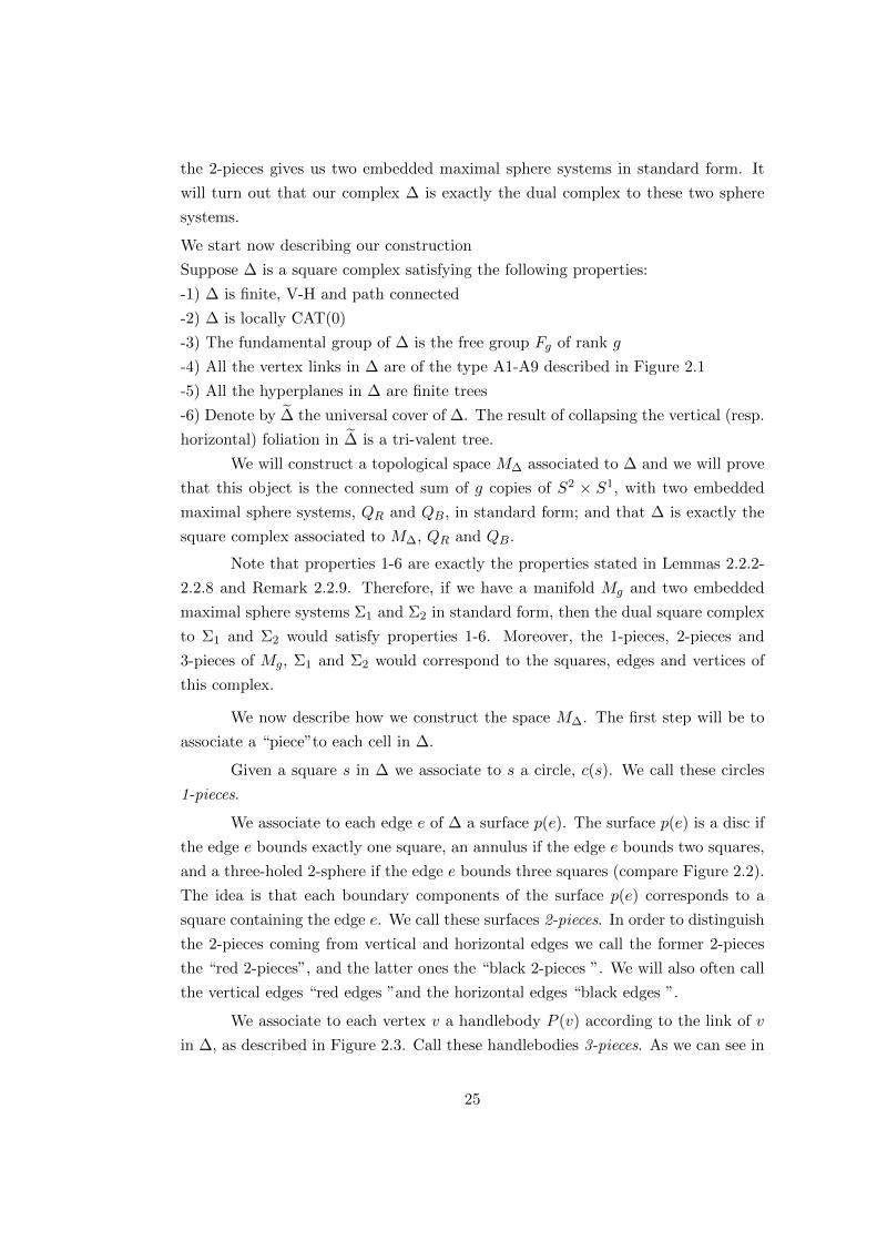
the 2-pieces gives us two embedded maximal sphere systems in standard form. It

will turn out that our complex ∆ is exactly the dual complex to these two sphere

systems.

We start now describing our construction

Suppose ∆ is a square complex satisfying the following properties:

-1) ∆ is finite, V-H and path connected

-2) ∆ is locally CAT(0)

-3) The fundamental group of ∆ is the free group Fg of rank g

-4) All the vertex links in ∆ are of the type A1-A9 described in Figure 2.1

-5) All the hyperplanes in ∆ are finite trees

-6) Denote by ∆ the universal cover of ∆. The result of collapsing the vertical (resp.

horizontal) foliation in ∆ is a tri-valent tree.

We will construct a topological space M∆ associated to ∆ and we will prove

that this object is the connected sum of g copies of S2 × S1, with two embedded

maximal sphere systems, QR and QB, in standard form; and that ∆ is exactly the

square complex associated to M∆, QR and QB.

Note that properties 1-6 are exactly the properties stated in Lemmas 2.2.2-

2.2.8 and Remark 2.2.9. Therefore, if we have a manifold Mg and two embedded

maximal sphere systems Σ1 and Σ2 in standard form, then the dual square complex

to Σ1 and Σ2 would satisfy properties 1-6. Moreover, the 1-pieces, 2-pieces and

3-pieces of Mg, Σ1 and Σ2 would correspond to the squares, edges and vertices of

this complex.

We now describe how we construct the space M∆. The first step will be to

associate a “piece”to each cell in ∆.

Given a square s in ∆ we associate to s a circle, c(s). We call these circles

1-pieces.

We associate to each edge e of ∆ a surface p(e). The surface p(e) is a disc if

the edge e bounds exactly one square, an annulus if the edge e bounds two squares,

and a three-holed 2-sphere if the edge e bounds three squares (compare Figure 2.2).

The idea is that each boundary components of the surface p(e) corresponds to a

square containing the edge e. We call these surfaces 2-pieces. In order to distinguish

the 2-pieces coming from vertical and horizontal edges we call the former 2-pieces

the “red 2-pieces”, and the latter ones the “black 2-pieces ”. We will also often call

the vertical edges “red edges ”and the horizontal edges “black edges ”.

We associate to each vertex v a handlebody P (v) according to the link of v

in ∆, as described in Figure 2.3. Call these handlebodies 3-pieces. As we can see in

25

discannulus 3-holed sphere

Figure 2.2: How to associate a 2-piece p(e) to an edge e. The edge we consider isthe black edge in the picture. The associated 2-piece is a disc if the edge boundsone square, an annulus if the edge bounds two squares, and a pair of pants if theedge bounds three squares.

the figure, each 3-pieces is endowed with a “boundary pattern”, i. e. the boundary

of the handlebody P (v) is a union of discs, annuli and three holed spheres, and these

surfaces are exactly the 2-pieces associated to the edges incident to v. The vertex

link determines how these 2-pieces are glued together to form the boundary of the

3-piece. Note that red and black 2-pieces alternate on the boundary of a 3-piece, i.

e. two 2-pieces of the same colour are never adjacent on the boundary of a 3-piece.

With a little abuse I will use the word 2-piece (resp 3-piece) to denote both

the open and closed surface (resp. handlebody).

The next step in order to construct the space M∆ is to glue all these pieces

together. The manifold M∆ will be constructed inductively, first taking the union of

the 1-pieces, then attaching the 2-pieces and eventually the 3-pieces. The procedure

is described below.

Let Ns be an indexing set for the squares of the complex ∆, Ne be an indexing

set for the edges of ∆ and Nv be an indexing set for the vertices of ∆.

Define C1 as the disjoint union of the circles c(si) for all i in the set Ns. We

can see C1 as a kind of 1-skeleton for M∆.

Then attach the 2-pieces to the 1-skeleton to form a 2-skeleton. Note that, if e

is an edge contained in the square s, then exactly one of the boundary components of

the 2-piece p(e) will correspond to the square s. We attach this boundary component

to the 1-piece c(s); the attaching map is meant to be a homeomorphism of the circle

to itself.

Denote by C2 the set C1⊔i∈Ne

p(ei) quotiented by the attaching maps and endowed

with the quotient topology. We choose the attaching maps in such a way that C2 is

orientable. Note that such a choice is possible and is unique up to isotopy. We may

see C2 as a kind of 2-skeleton for M∆.

Note that, by construction, C2 satisfies the following properties:

- Each boundary component of a 2-piece is attached to exactly one 1-piece,

and two different boundary components of the same 2-piece are attached to two

26

ball

solid torus

solid torus

complement

handlebody of genus 4

solid torus

genus two handlebody

genus two handlebody

complement

genus three handlebody

ball

C2

C3

C4

C5

C1 C6

C7

C8

C9

vertex link 3-piece vertex link 3-piece

Figure 2.3: How to associate to a vertex v the 3-piece P (v) with its “boundarypattern”. The general idea is the following: if G is the link of the vertex v in ∆,then each vertex of valence k in G corresponds to a planar surface having k boundarycomponents (where k is 1, 2 or 3); two surfaces are glued along a circle if and onlyif the two corresponding vertices are joined by an edge in the link G. This givesus the boundary pattern of the 3-piece P (v). Now, if the 3-piece is not a ball theboundary pattern yields two possible choices for the 3-piece P (v); in this case wepick the one where 1-pieces on the boundary are not all trivial in π1(P (v)). Thetable shows the vertex links and the associated 3-pieces. The 3-piece drawn in C1is a ball whose boundary is the union of two black discs and a red annulus. C2represents a solid torus whose boundary is the union of two black annuli and twored annuli. C3 represents a solid torus whose boundary is the union of three blackannuli and three red annuli. The 3-piece drawn in C4 represents a handlebody ofgenus 4 whose boundary is the union of three black 3-holed spheres and three red3-holed spheres, due to the difficulty in drawing the actual 3-piece, I have drawnthe complement of the 3-piece in S3. C5 represents a solid torus whose boundaryis the union of two black annuli, two red annuli and a black disc. C6 represents ahandlebody of genus 2 whose boundary is the union of two black annuli, two redannuli, a black 3-holed sphere and a red 3-holed sphere. C7 represents a handlebodyof genus 2 whose boundary is the union of three black annuli and two red 3-holedspheres. C8 represents a handlebody of genus 3 whose boundary is the union of twoblack 3-holed spheres, two red 3-holed spheres, a black annulus and a red annulus;in this case also, in view of the difficulty in drawing the actual 3-piece, I have drawnthe complement of the 3-piece in S3. C9 represents a ball whose boundary is theunion of a black disc, a red disc, a black annulus and a red annulus.

27

different 1-pieces.

- For each 1-piece c = c(s) exactly four different 2-pieces, two black ones and

two red ones, are glued to c, these are exactly the 2-pieces corresponding to the four

edges of the square s.

Now we need to glue the 3-pieces to the 2-skeleton C2.

Consider a vertex v in ∆ and consider all the edges and squares in ∆ which

are incident to v, take all the 2-pieces and 1-pieces in C2 corresponding to these

edges and squares, denote this union of pieces as the piece cycle induced by the

vertex v. Note that, since each vertex link in ∆ is connected, than each piece cycle

is connected; and that red and black 2-pieces alternate on each piece cycle. Note also

that each 2-piece belongs to exactly two piece cycles and that each 1-piece belongs

to exactly four piece cycles.

Since a piece cycle depends only on the link of the vertex it corresponds

to, then we can list all possible piece cycles, there are exactly nine possible cases,

which are the ones listed in Figure 2.3. Each piece cycle is a closed orientable surface,

therefore it bounds a handlebody, namely the 3-piece associated to the corresponding

vertex. Note that the piece cycle induced by the vertex v corresponds exactly to the

boundary pattern of the 3-piece P (v). Therefore we can attach the 3-pieces to C2.

To be precise, here the gluing maps are defined only up to Dehn twists around

the cores of the 2-pieces. For the moment we choose the gluing maps and carry on

with the construction. We will observe below (Remark 2.3.4) that a different choice

for the gluing maps would in the end give us a homeomorphic 3-manifold, and

therefore our choice is not relevant. The main ingredient for this remark will be

Lemma 2.3.3. This lemma implies that each curve entirely contained in a 2-pieces

bounds an embedded disc in the 3-manifold we obtain.

Denote by M∆ the union of C2 and the 3-pieces, quotiented by the attaching

maps. Denote by QB the union of 1-pieces and black 2-pieces, and by QR the union

of 1-pieces and red 2-pieces.

The rest of this section is aimed at proving the following:

Theorem 2.3.1. The space M∆ is the connected sum of g copies of S2 × S1. QR

and QB are two embedded maximal sphere systems in standard form with respect to

each other.

The proof of Theorem 2.3.1 consists of several steps.

Lemma 2.3.2. M∆ is a closed topological 3-manifold.

Proof. We will show that each point q in M∆ has a neighborhood homeomorphic to

R3.

28

If the point q belongs to the interior of a 3-piece than clearly it has a neighborhood

homeomorphic to R3.

Suppose that the point q belongs to the interior of a 2-piece p(e), associated to

an edge e. Then, since the edge e connects in ∆ two vertices, v1 and v2, the

surface p(e) must belong to the boundary of P (v1) and to the boundary of P (v2),

and furthermore the handlebodies P (v1) and P (v2) are glued together along p(e).

Therefore there exist a neighborhood U1 of q in P (v1) which is homeomorphic to

R3−, and a neighborhood U2 of q in P (v2) which is homeomorphic to R3

+; U1

and U2 are glued together along their common boundary, their union gives us a

neighborhood U of q in M∆ homeomorphic to R3.

Finally, suppose that q is contained in the 1-piece c(s) corresponding to the square

s. Let e1, e2, e3 and e4 be the four edges of s and let v1, v2, v3 and v4 be the four

vertices of s. Then q lies on the boundary of the four 2-pieces p(ei), which intersect

in the circle c(s), as well as on the boundary of the 3-pieces P (vj) for i, j = 1...4.

The 2-piece p(ei) lies on the boundary of the two handlebodies P (vi) and P (vi+1).

Now, choosing suitable neighborhoods of q in the four 3-pieces it belongs to, and

gluing them together, we can find a neighborhood of q in M∆ homeomorphic to R3.

We have just proved that M∆ is a 3-manifold without boundary. Now, M∆ is

compact because it is a finite union of compact spaces.

Lemma 2.3.3. Each connected component of QB or QR is an embedded sphere in

M∆.

Proof. By construction each 1-piece is an embedded circle in M∆ and each 2-piece

is an embedded surface. Again by construction, two different 2-pieces are either

disjoint or they are glued together along a 1-piece. Each 1-piece bounds exactly two

red 2-pieces and two black 2-pieces. Therefore QB and QR are embedded surfaces

in M∆, possibly disconnected. Note that each component of QR and QB has empty

boundary, otherwise there would be a 1-piece bounding only one 2-piece, which is

impossible by construction.

Two 2-pieces of the same colour are glued together along a 1-piece if and only

if the edges they correspond to are the two horizontal (or vertical) edges of the

same square. Therefore there is a bijective correspondence between the hyperplanes

perpendicular to black (resp. red) edges and the connected components of QB (resp.

QR). There is a systematic way to recover the components of QB and QR from the

hyperplanes. Namely, consider a hyperplane H as a graph embedded in R3 and take

a tubular neighborhood UH of H. The corresponding surface will be the boundary

of UH . Since T is a finite tree, then UH is a ball and its boundary is a sphere.

29

I will prove later (in the proof of Lemma 2.3.11) that each sphere is essential.

Remark 2.3.4. As promised, we observe now that, if we had chosen different gluing

maps for the 3-pieces, the manifold we obtained would be homeomorphic to M∆,

therefore the construction is well defined. Choosing a different attaching map for

a 3-piece would be the same as performing a Dehn surgery of kind (1,n) (longitude

preserving) on a tubular neighborhood of a boundary parallel curve in a 2-piece.

Lemma 2.3.3 implies that a curve lying entirely on a 2-piece bounds an embedded

disc in M∆; therefore a longitude preserving Dehn surgery on a tubular neighborhood

of such a curve would not modify the homeomorphism class of M∆.

We go on with the proof of Theorem 2.3.1

Lemma 2.3.5. For each 3-piece P , its fundamental group π1(P ) is supported on

the 2-piece components of its boundary; i. e. there exists a basis for π1(P ) so that

each generator γ is homotopic to a loop γ′ entirely contained in one of the 2-pieces

composing ∂P .

Proof. This can be checked case by case looking at Figure 2.3.

Lemma 2.3.6. For each 3-piece P , the inclusion P → M∆ induces a trivial map

on the level of fundamental groups.

Proof. By lemma 2.3.5 each element of π1(P ) can be represented as a product of

loops each of which lies entirely on a 2-piece belonging to ∂P . By lemma 2.3.3 each

2-piece lies on a sphere in M∆, therefore each loop entirely contained in a 2-piece is

trivial in π1(M∆).

We will now prove that the fundamental group of M∆ is the free group Fg

of rank g. The proof will consist of several steps.

Let ∆ be the universal cover of ∆. ∆ is again a connected V-H square complex,

it is not finite, but it is locally finite. Moreover ∆ satisfies properties 2, 4, 5 and

6. We can again construct a 3-manifold M∆

from ∆ in the same way as we have

constructed M∆ from ∆. M∆

may not be compact but it is still a 3-manifold without

boundary, moreover Lemma 2.3.3, Lemma 2.3.5 and Lemma 2.3.6 still hold for M∆

.

Again the union of black and red 2-pieces gives us two collections of disjoint spheres

embedded in M∆

, call these collections QB and QR.

We will first prove that M∆

is a covering space for M∆ and the deck transformation

group is the free group Fg (Lemma 2.3.7); then we will prove that M∆

is simply

connected (Lemma 2.3.8). Consequently M∆

is the universal cover of M∆ and the

30

latter manifold is the quotient of the former one by the action of the group Fg. As

a consequence the fundamental group of M∆ is the free group Fg.

Lemma 2.3.7. The manifold M∆

is a covering space for M∆; and QB (resp. QR)

is the entire lift of the sphere system QB (resp. QR). Moreover, the deck transfor-

mation group for the covering map is the free group Fg.

Proof. Denote by g : ∆ → ∆ the covering map. We will exhibit a particular way

of constructing M∆

and a covering map h : M∆→ M∆. Then we can conclude

observing that, again by Remark 2.3.4, the construction of M∆

is well defined.

Take a circle for each square in ∆ to build the 1-skeleton C1 of M∆

. This 1-skeleton

is clearly a covering space for the 1-skeleton of M∆, the covering map maps the circle

associated to a square s to the circle associated to the square g(s) homeomorphically.

Then lift the gluing maps for the 2-pieces and obtain a 2-skeleton C2 for M∆

. There

is an obvious covering map f : C2 → C2, where C2 is the 2-skeleton of M∆; the map

f maps the 2-piece corresponding to an edge e to the 2-piece corresponding to the

edge g(e) homeomorphically.

Finally we can lift the gluing maps for the 3-pieces to obtain the manifold M∆

.

The covering map f : C2 → C2 extends to a map h : M∆→ M∆ mapping the

3-piece corresponding to a vertex v to the 3-piece corresponding to the vertex g(v)

homeomorphically.

By construction, the union of black (resp. red) 2-pieces in M∆

is the entire lift of

the sphere system QR (resp. QB).

Again by construction there is a bijective correspondence between the deck trans-

formation group of the covering map g : ∆→ ∆ and the deck transformation group

of the covering map h : M∆→M∆, therefore the deck transformation group for the

covering map h is the free group Fg.

Lemma 2.3.8. M∆

is simply connected.

Proof. In order to prove this lemma we first construct a graph G embedded in M∆

.

Then we prove that each loop in the graph G is trivial in the fundamental group

of M∆

. Finally we prove that the fundamental group of M∆

is supported on the

graph G (i. e. for each loop l in M∆

there is a loop l′ homotopic to l and entirely

contained in G). We will make large use of the construction described below also in

the proof of Lemma 2.3.9.

Let us start constructing this embedded graph G. The graph G will be

isomorphic to the union of the 1-skeleton of ∆ and the hyperplanes of ∆. We can

31

imagine the graph G as the 1-skeleton of a kind of “binary subdivision ”for the

square complex ∆.

To build this graph G, we first build a subgraph G′, which is isomorphic to

the 1-skeleton of ∆. Then we add the other vertices and edges.

We start constructing the graph G′. First recall that M∆

is obtained by

gluing together 3-pieces, 2-pieces and 1-pieces.

For each 3-piece P in M∆

take a point qP lying in the interior of the piece

P . These points will be the 0-skeleton of the graph G′. A 2-piece p in M∆

lies on

the boundary of exactly two 3-pieces, call them P1 and P2; draw an arc ap joining

the points qP1 and qP2 and intersecting only one 2-piece (the 2-piece p) in exactly

one point. After drawing an arc for each 2-piece, we obtain the graph G′ we were

looking for. Note that, by construction, G′ is isomorphic to the 1-skeleton of ∆.

Hence the shortest circuits in G′ are loops consisting of the concatenation of four

edges. We will use the term “4-circuits”to denote such circuits.

Now we build the graph G, the idea is that for each 4-circuit in G′ we take

a new vertex, and we join the midpoints of the four vertices composing the circuit

to this new vertex. Note that the midpoints of edges in G′ will become vertices in

the graph G.

We explain the construction more closely. Consider a 4-circuit in the graph

G. This circuit corresponds to four 2-pieces p1, p2, p3 and p4 in M∆

intersecting in

a 1-piece c.

Denote by ei the edge in G′ dual to the 2-piece pi. Take a point q in the

circle c. For each i = 1...4 take an arc βi entirely contained in the 2-piece pi and

joining the point q to the edge ei (see Figure 2.4). After doing this for each 4-circuit

in G′, we obtain the graph G we were looking for.

We will use the word newedges to denote the edges in G \G′. We can colour

each newedge with red or black according to the colour of the 2-piece the newedge

belongs to. We will use the word bisectors to denote the union of newedges belonging

to the same sphere in QR or QB. Note that, if the edges in the graph G′ inherit their

colour from the 2-pieces they intersect, then black bisectors in G are perpendicular

to black edges and red bisectors in G are perpendicular to red edges.

Note also that bisectors correspond exactly to hyperplanes in ∆ and that

each black (resp. red) bisector is a tree embedded in a component σ of QB (resp

QR). This tree has a vertex for each 2-piece lying on the sphere σ and an edge for

each 1-piece on the sphere σ.

We have constructed the graph G. We show now that each circuit in the

graph G is trivial in the fundamental group of M∆

. It is sufficient to show this

32

Figure 2.4: A 4-circuit in the graph G′ and the newedges. The dotted lines representthe newedges

for 4-circuits. To see this we observe that, by construction, each 4-circuit in G is

entirely contained in a single 3-piece of M∆

, and therefore, by Lemma 2.3.6 is trivial

in π1(M∆

).

To conclude the proof we only need to show that for each loop l in M∆

there

exists a loop l′ homotopic to l which is contained in the graph G. We can actually

say a bit more: in fact each loop is homotopic to a loop contained in the subgraph

G′.

Let l be a loop in M∆

. First note that up to homotopy, we can suppose that

l does not intersect any 1-piece, and that it intersects transversely every 2-piece.

We may as well suppose that l intersects a 2-piece pi, if at all, just in the only

intersection point between the 2-piece pi and the graph G′. As a consequence of

Lemma 2.3.6, two paths contained in the same 3-piece and with the same endpoints

are homotopic in M∆

relatively to their boundary. Therefore, up to homotopy, we

can suppose that l is contained in the graph G′ constructed above.

The construction explained in the proof of Lemma 2.3.8 is very useful to

prove the following:

Lemma 2.3.9. The complementary components of QB and the complementary com-

ponents of QR in M∆

are three holed 3-spheres.

Proof. We prove that each complementary component of QB in M∆

is a three holed

3-spheres. The same holds true for complementary components of QR.

Let C be a component ofM∆\QB. Note that C is a 3-manifold with boundary

and its boundary consists of a certain number of spheres. The plan is to prove that C

is simply connected, compact, and has exactly three boundary components. Then,

using Poincare conjecture, we deduce that C is a 3-holed 3-sphere. As mentioned,

we will use the construction (and the notation) explained in the proof of Lemma

2.3.8.

33

Recall that we constructed a graph G embedded in the manifold M∆

. If we

look at that construction closely we note that the intersection between a component

of QB and the graph G is exactly a black bisector in the graph G. Consequently the

intersections between G and the components of M∆\ QB are the complementary

components of black bisectors in G. Denote by C the graph C ∩G.

We first show that C is simply connected.

Using the same argument as in the proof of Lemma 2.3.8, we can show that

each loop in C is homotopic to a loop in the graph C.

We can also show that each loop in the graph C is trivial in the fundamental

group of C.

Again it is sufficient to show this for 4-circuits in the graph C.

We have shown in the proof of Lemma 2.3.8 that each 4-circuit of C is entirely

contained in a single 3-piece of C.

Now note that, for each 3-piece P , there is a basis of the fundamental group π1(P )

so that each element in this basis is homotopic to a 1-piece. This can be easily

checked case by case by looking at Figure 2.3.

We conclude observing that each 1-piece is trivial in the fundamental group of C,

since it lies on one of the boundary spheres.

It follows that C is simply connected.

Since hyperplanes are finite in ∆, then bisectors are finite in the graph G;

consequently the component C is compact, because it is the union of a finite number

of 3-pieces.

We only need to show that C has exactly three boundary components. To

see this note that, by property 6) on page 24, by collapsing ∆ along the red edges,

we obtain a trivalent tree; this means that, by collapsing each red edge and each

black bisectors in the graph G to a point, we obtain a trivalent tree. This implies

that each complementary component of black bisectors in G is bounded by exactly

three hyperplanes, and therefore, each complementary component C of QB in M∆

is bounded by exactly three spheres.

Summarising, C is compact, simply connected and bounded by three 2-

spheres, this means that C is a three-holed 3-sphere. The same argument works

for the complementary components of QR.

While proving Lemma 2.3.9 I used Poincare conjecture. I believe there is a

way of proving it which does not use Poincare conjecture, and I will think about

that as a future project.

Lemma 2.3.7 and lemma 2.3.8 immediately imply the following:

34

Lemma 2.3.10. M∆

is the universal cover of M∆. M∆ is the quotient of M∆

by

the action of the free group Fg. In particular, the fundamental group of the manifold

M∆ is the free group Fg.

Now, M∆ is a close 3-manifold whose fundamental group is the free group

Fg, hence it has to be the connected sum of g copies of S2 × S1 (compare [18] 5.3

for a reference).

Again, while asserting this I am using Poincare conjecture. As a future

project I will look for a way to avoid the use of Poincare conjecture.

In order to finish the proof of Theorem 2.3.1 we only need to prove the

following:

Lemma 2.3.11. Each component of QR and QB is an essential sphere in M∆.

Moreover QR and QB are maximal sphere systems in M∆ in standard form with

respect to each other.

Proof. It is easier to prove Lemma 2.3.11 by analysing the situation in the universal

cover M∆

. As above, denote by QR and QB the full lifts of QR and QB in the

universal cover M∆

of M∆.

We have proved (Lemma 2.3.9) that each component of M∆\ QB and of

M∆\ QR is a three holed 3-sphere. This means that each component of M∆ \ QB

and of M∆ \ QR is a three holed 3-sphere As a consequence QB (resp. QR) is

a maximal collection of disjoint non pairwise isotopic essential spheres, i. e. a

maximal sphere system.

We only need to prove that the systems QR and QB are in standard form.

Recall that this means that QR and QB are in strong minimal form (i. e. each sphere

in QB intersects each sphere in QR minimally) and the complementary components

of QR ∪QB in M∆ are handlebodies.

We show first that QR and QB are in strong minimal form. We will show

this by using the properties of the complex ∆. Recall that components of QR and

QB naturally correspond to hyperplanes in ∆.

First note that the square complex ∆ is simply connected and locally CAT(0);

therefore, by a generalisation of Cartan-Hadamard Theorem ([5] p. 193), ∆ is

CAT(0). By the discussion in Section 2.2 two hyperplanes in a CAT(0) cube complex

intersect at most once. Consequently two hyperplanes in ∆ intersect at most once.

As a consequence, a component of QR and a component of QB can intersect at

most once. Moreover the complex ∆ is constructed in such a way that no 3-piece

is bounded by two disks. These two facts imply that each sphere in QR intersects

35

each sphere in QR minimally, and therefore the sphere systems QR and QB are in

strong minimal form.

Since, by construction, the complementary components of QR⋃QB are han-

dlebodies, then the systems QR and QB are in standard form.

This concludes the proof of Theorem 2.3.1.

Remark 2.3.12. Note that if we apply the construction described in Section 2.2 to

the manifold M∆ (resp. M∆

), we obtain the complex ∆ (resp. ∆). Therefore ∆

(resp. ∆) is the dual square complex associated to M∆, QB, QR (resp. to M∆

, QB,

QR).

A consequence of the constructions described in Section 2.2 and in Section

2.3 is the following:

Lemma 2.3.13. Let Mg, M′g be connected sums of g copies of S2×S1. Let Σ1, Σ2

be two maximal sphere systems embedded in Mg, containing no spheres in common

and in standard form with respect to each other. Let Σ′1, Σ′2 be two maximal sphere

systems embedded in M ′g, containing no spheres in common and in standard form

with respect to each other. Suppose the square complex associated to Mg, Σ1, Σ2

is isomorphic to the square complex associated to M ′g, Σ′1, Σ′2. Then there exists a

homeomorphism F : Mg →M ′g such that F (Σi) is Σ′i for i = 1, 2.

Proof. Let us denote by ∆ the square complex dual to Mg, Σ1 and Σ2 and by ∆′

the square complex dual to M ′g, Σ′1 and Σ′2.

As observed in Section 2.2, the manifolds Mg and M ′g can be constructed by

gluing together 1-pieces, 2-pieces and 3-pieces. These pieces correspond to squares,

edges and vertices in the complexes ∆ and ∆′.

The isomorphism of square complexes induces a bijective correspondence f

between the pieces of Mg and the pieces of M ′g. Each piece P in Mg is homeomorphic

to the piece f(P ). Moreover, the correspondence f respects the boundary relations

(i. e. an n-piece p lies on the boundary of an (n+1)-piece P if and only if the n-piece

f(p) lies on the boundary of the (n+1)-piece f(P)).

We can therefore construct the homeomorphism F piece by piece as explained

below.

There is a natural homeomorphism F ′ from the collection of 1-pieces of Mg

to the collection of 1-pieces of M ′g mapping a 1-piece to the corresponding one

homeomorphically.

Since the correspondence f respects the boundary relations, then the home-

omorphism F ′ extends to a homeomorphism F ′′ : Σ1 ∪ Σ2 → Σ′1 ∪ Σ′2.

36

Now, Mg is obtained by gluing 3-pieces to Σ1 ∪ Σ2 and M ′g is obtained by

gluing 3-pieces to Σ′1 ∪ Σ′2.

We would like to extend the homeomorphism F ′′ to the 3-pieces. The gluing

maps of the 3-pieces might be different, in fact, they might differ by Dehn twists

around curves in 2-pieces. Therefore, before extending the homeomorphism F ′′ to

3-pieces we might have to perform a finite number of surgery operations in Mg.

These surgery operations consist of removing a 3-piece and gluing it again

through a different gluing map on the boundary. As observed in Remark 2.3.4, this

operation corresponds to a Dehn surgery of kind (1, n) in Mg, on the tubular neigh-

borhood of a loop bounding an embedded disk. As a consequence, after performing

such a surgery, we obtain a manifold homeomorphic to Mg. Moreover such a Dehn

surgery may be performed in such a way that it fixes spheres in Σ1 and Σ2 and

therefore the homeomorphism between Mg and the manifold we obtain after the

surgery fixes each piece setwise.

Therefore, after performing a finite number of trivial Dehn surgeries on Mg,

we obtain a manifold M ′′g with the same pieces as Mg and different gluing maps.

Now the homeomorphism F ′′ extends to F ′′′ : M ′′g →M ′g.

The homeomorphism F is given by the composition of F ′′′ and the surgery

operations.

Note in particular that the isomorphism between the two square complexes

induces a bijective correspondence between the vertical (resp. horizontal) hyper-

planes of the two complexes, and this correspondence between hyperplanes induces

a bijective correspondence between spheres in Σ1 (resp. Σ2) and spheres in Σ′1 (resp.

Σ′2). The homeomorphism F : Mg →M ′g respects this correspondence.

2.4 The core of two trees

In this section we describe an abstract construction. Starting with two trees and

two group actions by the free group Fg on these trees, we will construct a square

complex C and denote it as the core of the two trees. We will then prove that a

quotient of the complex C by the action of the group Fg satisfies all the six properties

mentioned in Section 2.3. Therefore, by theorem 2.3.1 we can associate to it a 3-

manifold Mg with two embedded maximal sphere systems in standard form. In

other words the complex C is the universal cover of a square complex ∆ satisfying

properties 1-6 of section 3, therefore we can associate to C a 3-manifold Mg with

two embedded maximal sphere systems. The connection between the complex we

describe in this section and the one we described in Section 2.2 will be explained

37

in the next section. Namely in Theorem 2.5.1 we prove that the method described

below is just an abstract way of constructing the square complex described in Section

2.2.

One can check that the complex C we construct coincides with the “Guirardel

core”of the two trees, defined in [10]. However, our definition will be different from

the one given in [10]. Compare [22] Section 1.2, and 2.1 for a slightly different

definition of Guirardel Core and some ideas on why this Core is related to the

intersection of two sphere systems.

We start describing our construction.

Let T and T ′ be two three-valent trees both endowed with a free, properly

discontinuous and cocompact action by the free group Fg, call these actions ρ and

ρ′.

Since the group Fg acts freely and properly discontinuously on the tree T ,

then the boundary of T can be canonically identified to the boundary of Fg. To

understand how this identification works first note that the elements of the Gromov

boundary of Fg correspond to the infinite words in Fg; let w be an infinite word and

let us denote by wn the prefix of w of length n. We associate then to the word w

the shortest quasi-geodesic ray in T containing the points ρwn(x) for each natural

number n, where x is any point in T . Note that, since ρh is an isometry for each h

in Fg, if x and x′ are two different points in T , then for each natural number n the

distance between ρwn(x) and ρwn(x′) is equal to the distance between x and x′, and

the identification described above does not depend on the choice of the point x.

In the same way, the action of the group Fg on the tree T ′ induces a canonical

identification of the Gromov boundary of T ′ to the Gromov boundary of Fg.

Consequently, the Gromov boundary of T can be naturally identified to the

Gromov boundary of T ′, since they can both be identified to the Gromov boundary

of the group Fg. For this reason in the remainder, abusing notation, I will often

use the term “boundary of T ”to refer to both the Gromov boundary of T and the

Gromov boundary of T ′, and sometimes I will write ∂T in order to abbreviate.

Each edge in T (resp. T ′) induces a partition on the Gromov boundary of

T (which coincides with the Gromov boundary of T ′). If e is an edge in T , we

will denote by Pe the partition induced by e on ∂T and by e+ and e− the two sets

composing this partition.

If e is an edge in T and e′ is an edge in T ′, we say that the induced partitions

Pe and Pe′ are non nested if no set of one partition is entirely contained in a set of

the other partition, namely all the sets e+ ∩ e′+, e+ ∩ e′−, e− ∩ e′+, e− ∩ e′− are all

38

non empty. We say that the induced partitions are nested otherwise.

In the remainder we will assume the following:

(*) There do not exist an edge e in T and an edge e′ in T ′ inducing the same

partition on the Gromov boundary.

We will see in Section 2.5 that supposing hypothesis (*) corresponds the

assumption, made in the previous sections, that two sphere systems do not contain

spheres in common.

Consider now the topological space T × T ′, this space is a CAT(0) square

complex, where each vertex link is the bipartite graph K3,3. This space can be

naturally endowed with a diagonal action γ. Namely, given a vertex (v1, v2) in

T × T ′ and an element g of Fg, we set γg(v1, v2) to be the vertex (ρg(v1), ρ′g(v2)).

Since ρ and ρ′ are free and properly discontinuous, also γ is. The quotient space

(T × T ′)/Fg is a locally CAT(0) square complex whose fundamental group is Fg,

but it may not be compact.

We define now the main object of this section.

Definition 2.4.1. The core of T and T ′ is the subcomplex of T×T ′ consisting of all

the squares e×e′ where e is an edge in T , e′ is an edge in T ′, and the two partitions

induced by e and e′ on the boundaries of T and T ′ are not nested. We will denote

this complex by C(T, T ′). Where no ambiguity can occur, I will write C instead of

C(T, T ′).

Remark 2.4.2. Note that we can define the core of two trees also in a more general

setting. Namely, we do not really need two group actions, we use them only because

they define a boundary identification. We could define the core just starting with two

trees T and T ′, and any identification between the boundary of T and the boundary

of T ′.

In the remainder of this section we describe some of the properties of the

complex C. The aim is to show that the complex C is invariant under the diagonal

action of the group Fg and the quotient of the complex C by this group action

satisfies all the six properties stated in the previous section. We start proving the

following:

Proposition 2.4.3. The complex C is invariant under the diagonal action of the

group Fg.

Proof. To see that C is invariant under the action of Fg, note that for each g in Fg

the maps ρg and ρ′g induce the same homeomorphism on ∂T = ∂T ′, therefore, the

39

partitions induced by the edges e and e′ are nested if and only if the ones induced

by the edges ρg(e) and ρ′g(e′) are.

Before stating the next lemma, I need to clarify some terminology which will

be used throughout this section. Recall that the complex C is a subcomplex of the

product T × T ′, therefore C is endowed with two projections: πT : C → T and

πT ′ : C → T ′.

If e is an edge in T , by the term preimage of the edge e, I will denote the

preimage of the edge e under the map πT : C → T . Analogously, if e′ is an edge in

T ′, by the term preimage of the edge e′, I will denote the preimage of the edge e′

under the map πT ′ : C → T ′. Same for preimages of vertices.

With this terminology in mind we can state the following:

Lemma 2.4.4. The preimage of each edge is the trivial interval bundle over a finite

tree, in particular it is connected and finite.

Proof. We will only prove this for edges in T , and the same arguments will hold for

edges in T ′. If e is an edge in T denote by Fe the preimage of e. Note that Fe is the

interval bundle over the set of edges e′ in T ′ such that the partitions induced by e

and e′ are not nested; denote by T ′e this subset of T ′. The edge e′ belongs to T ′e if

and only if all the sets e′+ ∩ e+, e′− ∩ e+, e′+ ∩ e− and e′− ∩ e− are non empty. We

will prove that T ′e is a finite subtree of T ′.

We first prove that for each edge e in T its preimage Fe is connected, or

equivalently T ′e is connected. To prove this we will show that if two edges a and b

in T ′ belong to T ′e, then the geodesic in T ′ joining a and b is contained in T ′e. We

may suppose without losing generality a+ ⊃ b+. Consider any edge c in the geodesic

joining a and b; we may suppose a+ ⊃ c+ ⊃ b+, and as a consequence a− ⊂ c− ⊂ b−.

Now, since the sets b+ ∩ e+ and b+ ∩ e− are non empty, then the sets c+ ∩ e+ and

c+ ∩ e− are respectively non empty; since the sets a− ∩ e+ and a− ∩ e− are non

empty, then the sets c− ∩ e+ and c− ∩ e− are also non empty. Hence, the edge c

belongs to T ′e, which is what we need to prove.

We prove now that, for each edge e in T , its preimage Fe is finite (or equiv-

alently T ′e is finite) , which is equivalent to saying that, given an edge e in T , there

are only finitely many edges e′i in T ′ such that the partitions on ∂T induced by e

and e′i are not nested.

If e is an edge in T and e′i is an edge in T ′ denote as usual by e+ and e− the two

sets of the partition induced by e, and by e′i+ and e′i

− the two sets of the partition

induced by e′i.

40

First we claim that if r′ = {e′i} with i ∈ N is a geodesic ray in T ′, then the subset of

r′ contained in Fe is finite. Note that by connectedness of the edge preimages, this

subset is either a finite segment or a subray of r′. Therefore, in order to prove the

claim, it is sufficient to prove that there exists I ∈ N such that the set e′i+ (or e′i

−)

is contained in one of the two sets e+ or e− for each i ≥ I.

To prove this, note that the limit of the ray {e′i} is a point in ∂T ′; this point belongs

either to e+ or to e−, we may suppose it belongs to e+. Now suppose that both sets

e+i ∩ e+ and e+

i ∩ e− are non empty for each i; then, since these are compact subsets

of the compact space ∂T ′, both the sets (∩i∈Ne+i ) ∩ e+ and (∩i∈Ne+

i ) ∩ e− are non

empty, but this is absurd because (∩i∈Ne+i ) is a point in ∂T ′ belonging to e+.

We have proved above that the set of edges {e′i ∈ T ′ : e′ ∈ T ′e} is a connected subtree

of T ′. Now suppose that T ′e contains infinitely many edges of T ′, by connectedness

it would contain a geodesic ray, which leads to a contradiction.

An immediate consequence of Lemma 2.4.4 is the following:

Corollary 2.4.5. Hyperplanes in C(T, T ′) are finite trees.

Another consequence of Lemma 2.4.4 is the following:

Proposition 2.4.6. The quotient space C/Fg is a finite square complex.

Proof. By invariance of the core, if e is any edge in T , g is any element of Fg, and

Fe is the preimage of the edge e in C(T, T ′), then the preimage Fρg(e) of the edge

ρg(e) is exactly γg(Fe), where γ is the diagonal action by the group Fg. Moreover,

since the actions of the group Fg on the trees T and T ′ are free, then two squares

belonging to the preimage of the same edge cannot be identified under the quotient

map.

Since the actions ρ is cocompact, then T/Fg is a finite graph. By Proposition 2.4.4

each edge preimage contains a finite number of squares. Therefore C/Fg is a finite

square complex. In particular C/Fg is compact.

Remark 2.4.7. Note that the square complex C is V-H by construction, since it is

a subcomplex of the product of two trees. The quotient C/Fg is also V-H, since the

diagonal action of the group Fg sends vertical (resp. horizontal) edges to vertical

(resp. horizontal) edges.

The next goal will be proving the following:

Proposition 2.4.8. The complex C is connected.

41

Proof. The proof consists of several steps. Note that in this proof we strongly use

the hypothesis (*) on page 39, i. e. we suppose that there do not exist an edge in

T and an edge in T ′ inducing the same partition. The first step consists in proving

the following:

Lemma 2.4.9. The projections πT : C → T and πT ′ : C → T ′ are both surjective.

Proof. We prove that πT is surjective, i. e. for each edge e in T there exists an edge

e′ in T ′ such that e× e′ is in C or equivalently such that the partition induced by e

and the one induced by e′ are non nested. The same argument can be used to prove

that the projection πT ′ is surjective. Let e be any edge in T . As usual we denote

by Pe = e+ ∪ e− the partition induced by the edge e.

First we claim that there are edges a and b in T ′ such that a+ ⊂ e+ ⊂ b+.

To prove the claim note first that, since by Corollary 2.4.5 the preimage Fe is finite,

there is at least one edge a in T ′ such that the partitions Pe and Pa are nested.

We may suppose without losing generality a+ ⊂ e+. Pick a point p in e− and let

r = a, e′1, e′2... be the geodesic ray in T ′ joining the edge a to the point p. Since we

have e− ⊂ a−, the point p belongs to a−. Consequently we have the containment

e′+i ⊂ e′+i+1 for each ei

′ in the geodesic ray r. The set⋃i e′+i coincides with ∂T ′ \ p,

and therefore it contains e+. Since e+ is compact, there exists a natural number

I such that e′+i contains e+ for each i greater than or equal to I. We choose I to

be minimal among the numbers having this property. The edge e′I is what we were

looking for. Denote e′I by b. This proves the claim.

We will now use this claim to find an edge e′ in T ′ such that the partitions

induced by e and e′ are not nested. If we use the same notation as above this edge

will be one of the two edges adjacent to b.

Let a and b be the edges of T ′ defined above and let r be the geodesic defined above.

Denote by c the edge immediately preceding b on the ray r. We know that c+ ⊂ b+,

that b+ ⊃ e+, and that c+ does not contain e+ (this follows from the fact that b is

the first edge in the ray r such that b+ contains e+). Recall that no containment

can be an equality. There are then two possibilities.

-The first one is c+ * e+. In this case the partition induced by e and the one

induced by c are not nested.

-The second possibility is c+ ⊂ e+. In this case call d the edge in T ′ adjacent to

both b and c and denote by v the vertex in T ′ where the edges c, b, d intersect.

We will prove that the partitions induced by d and e are not nested. The vertex

v induces a partition ∂T ′ = D1 ∪ D2 ∪ D3 where D1 is equal to c+, D2 is equal

to b− and D3 is equal to ∂T ′ \ (D1 ∪ D2). Therefore the partition induced by d

42

is ∂T ′ = (D1 ∪ D2) ∪ D3. Now, since e+ strictly contains c+ = D1 and is strictly

contained in D1 ∪ D3 = b+, both the sets e+ ∩ D3 and e− ∩ D3 are non empty.

Moreover, since D1 is contained in e+ the set (D1 ∪ D2) ∩ e+ is non empty; and

since e+ is contained in b+ = D1 ∪D3 then D2 is contained in e− and therefore the

set (D1 ∪D2) ∩ e− is non empty. Consequently the partitions induced by e and d

are non nested, which is what we need to prove.

Using the same argument we can show that the projection πT ′ : C → T ′ is

surjective.

Lemma 2.4.10. The preimage of each vertex is a finite tree, in particular it is

connected.

Proof. We prove that for any v in T its preimage, denote it by Fv, is a finite tree.

One can use the same argument to prove that the preimage of any vertex in T ′ is a

finite tree.

Let v be any vertex in T and denote by e1, e2 and e3 the three edges incident to

the vertex v. The preimage Fv is the union of the edges in T ′ belonging to the

preimages of e1, e2 and e3. By Lemma 2.4.4 the space Fv is a union of three finite

trees; therefore, to prove Lemma 2.4.10, we only need to prove that Fv is connected.

First we state a necessary and sufficient condition for an edge in T ′ to belong

to Fv. Then we show that the set of edges in T ′ satisfying this condition is connected.

To state the condition, note first that v induces a partition of ∂T given by

∂T = D1 ∪ D2 ∪ D3. If e1, e2 and e3 are as above then e1 induces the partition

∂T = D1 ∪ (D2 ∪D3), e2 induces the partition ∂T = D2 ∪ (D1 ∪D3) and e3 induces

the partition ∂T = (D1∪D2)∪D3; compare Figure 2.5. We claim that an edge e′ in

T ′ belongs to Fv if and only if neither of the sets e′+ and e′− is entirely contained in

any of the Dis. Note that the fact that there are not two edges inducing the same

partition implies that it is not possible to have e′+ = Di or e′− = Di for any i. Now

we prove the claim.

The “only if ”is straightforward, in fact if e′+ (or e′−) is contained in one of the Dis

then the partition induced by e′ and the one induced by ej would be nested for each

j = 1, 2, 3.

Let us prove now that, if for each i = 1, 2, 3 we have e′+ * Di and e′− * Di then

there exists an i such that the partition induced by e′ and the one induced by ei are

not nested, i. e. there exists an i such that all the sets e′+∩Di, e′−∩Di, e

′+∩DiC ,

e′− ∩DiC are non empty. To prove this, note first that there exists an i such that

both sets e′+ ∩Di and e′− ∩Di are non empty, in fact, if this were not true, there

43

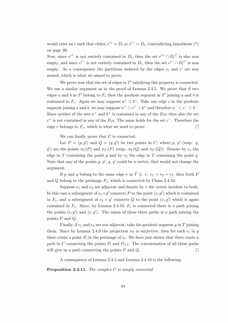
would exist an i such that either e′+ = Di or e′− = Di, contradicting hypothesis (*)

on page 39.

Now, since e′+ is not entirely contained in Di, then the set e′+ ∩ DiC is also non

empty, and since e′− is not entirely contained in Di, then the set e′− ∩DiC is non

empty. As a consequence the partitions induced by the edges ei and e′ are non

nested, which is what we aimed to prove.

We prove now that the set of edges in T ′ satisfying this property is connected.

We use a similar argument as in the proof of Lemma 2.4.5. We prove that if two

edges a and b in T ′ belong to Fv then the geodesic segment in T ′ joining a and b is

contained in Fv. Again we may suppose a+ ⊃ b+. Take any edge c in the geodesic

segment joining a and b, we may suppose a+ ⊃ c+ ⊃ b+ and therefore a− ⊂ c− ⊂ b−.

Since neither of the sets a+ and b+ is contained in any of the Dis, then also the set

c+ is not contained in any of the Dis. The same holds for the set c−. Therefore the

edge c belongs to Fv, which is what we need to prove.

We can finally prove that C is connected.

Let P = (p, p′) and Q = (q, q′) be two points in C, where p, p′ (resp. q,

q′) are the points πT (P ) and πT ′(P ) (resp. πT (Q) and πT ′(Q)). Denote by e1 the

edge in T containing the point p and by e2 the edge in T containing the point q.

Note that any of the points p, p′, q, q′ could be a vertex, that would not change the

argument.

If p and q belong to the same edge e in T (i. e. e1 = e2 = e), then both P

and Q belong to the preimage Fe, which is connected by Claim 2.4.10.

Suppose e1 and e2 are adjacent and denote by v the vertex incident to both.

In this case a subsegment of e1×p′ connects P to the point (v, p′) which is contained

in Fv, and a subsegment of e2 × q′ connects Q to the point (v, q′) which is again

contained in Fv. Since, by Lemma 2.4.10, Fv is connected there is a path joining

the points (v, p′) and (v, q′). The union of these three paths is a path joining the

points P and Q.

Finally, if e1 and e2 are not adjacent, take the geodesic segment g in T joining

them. Since by Lemma 2.4.9 the projection πT is surjective, then for each ei in g

there exists a point Pi in the preimage of ei. We have just shown that there exists a

path in C connecting the points Pi and Pi+1. The concatenation of all these paths

will give us a path connecting the points P and Q.

A consequence of Lemma 2.4.4 and Lemma 2.4.10 is the following:

Proposition 2.4.11. The complex C is simply connected

44

v

e1

e2e3

D1

D2 D3

v'

e1'

e2'e3'

D1'

D2' D3'

Figure 2.5: Partition induced by a vertex

Proof. Any loop l in C would project, by compactness, to a finite subtree of T ,

therefore, in order to prove that C is simply connected, it is sufficient to show that,

for any finite subtree S of T , the preimage π−1T (S) (which we denote as FS), is

simply connected.

Now note that, if S is a finite subtree of T , then FS is the union over all the

edges e and all the vertices v in S of the preimages Fe and Fv. Note also that by

Lemma 2.4.4 each edge preimage is connected and simply connected, and by Lemma

2.4.10 each vertex preimage is a finite tree. Moreover, the preimage Fe of an edge

e and the preimage Fv of a vertex v, intersect if and only if the vertex v is one of

the endpoints of the edge e, and in that case the intersection is a finite tree. Now,

using an inductive argument and Van Kampen theorem, it is easy to check that FS

is simply connected.

As a consequence of Proposition 2.4.11, the fundamental group of the quo-

tient C/Fg is the free group Fg.

Now compare the six properties stated on page 24. We have proven so far

that the complex C/Fg satisfies property 1 (by Proposition 2.4.6, remark 2.4.7 and

Proposition 2.4.8); property 3; and property 5 (by Corollary 2.4.5) By construction

and by Lemma 2.4.9, the complex C/Fg satisfies property 6 also. Moreover, since

the complex C is a subcomplex of the product T × T ′, then each vertex link is a

subgraph of the bipartite graph K3,3, therefore the complex C/Fg is locally CAT(0),

this means that C/Fg satisfies property 2. The next step is to understand how the

vertex links look like in C/Fg, or equivalently in C. For the sake of simplicity we

will investigate vertex links in C.

45

First note that, the complex C is contained in the product T × T ′ and all

vertex links in T×T ′ are isomorphic to the complete bipartite graph K3,3. Therefore,

if V = (v, v′) is a vertex in C, then its link has to be a subgraph of the bipartite

graph K3,3.

More precisely, consider a vertex (v, v′) in T ×T ′. The vertex v is incident in

T to three edges: e1, e2 and e3. The vertex v′ is incident in T ′ to three edges: e′1, e′2and e′3. The square ei×e′j belongs to the core C if and only if the partitions induces

by the edges ei and e′j are not nested. Therefore the link of the vertex (v, v′) will

consist of two sets of at most three vertices: a black set representing the edges e1, e2

and e3 and a red set representing the edges e′1, e′2 and e′3. There is an edge joining

the ith black vertex to the jth red vertex if and only if the partitions induces by

the edges ei and e′j are not nested.

We analyse systematically all the possibilities for vertex links in C. To do

this, we associate to a given vertex (v, v′) in T × T ′ a 3× 3 table. The task of this

“vertex table”is to give us information on the i’s and j’s for which the partitions

induced by the edges ei and e′j are non nested. Then we can deduce the vertex link

from the table associated to a given vertex. Note that the link of a vertex (v, v′)

might turn out to be empty. In this case the vertex (v, v′) is not in the core C.

We explain below how we construct the table for a given vertex (v, v′)

First note that the vertex v is incident in T to three edges e1, e2, e3 and

induces on the boundary a partition ∂T = D1 ∪D2 ∪D3. The edge e1 induces the

partition ∂T = D1∪(D2∪D3); the edge e2 induces the partition ∂T = D2∪(D1∪D3);

the edge e3 induces the partition ∂T = (D1∪D2)∪D3; as shown in Figure 2.5. The

same holds for the vertex v′ in T ′.

This is how we draw the table for the vertex (v, v′): we draw a cross in the

slot (i, j) if the set Di ∩D′j is non empty, we draw a circle in the slot (i, j) if the set

Di ∩D′j is empty. In the caption to Figure 2.7 we explain how to deduce from the

position of crosses and circles whether, for i, j = 1, 2, 3, the partitions induced by

the edges ei and e′j are nested.

It is not difficult to analyse systematically all the possible vertex tables.

These are 3 by 3 tables whose entries can be only crosses or circles. Moreover,

they have to satisfy some additional condition: first, since ∂T = D1 ∪ D2 ∪ D3 =

D′1 ∪D′2 ∪D′3, there has to be at least a cross in each row and column of the table;

second, since we assumed that there are no edges inducing the same partition, then

the union of a row and a column must contain at least two crosses (see Figure 2.6

for an example of these “forbidden patterns”). Furthermore permuting the order of

rows or columns in the table, or reflecting the table through the diagonal would not

46

Figure 2.6: The patterns drawn above are “forbidden”in vertex tables. In fact, thepattern on the left hand side of the figure would imply that ∂T is empty; the patternin the center would imply D1 = D′1, consequently e1 and e′1 would induce the samepartition, contradicting hypothesis (*) on page 39; the pattern on the right handside of the figure would imply D1 = D′2 ∪D′3, contradicting again hypothesis (*) onpage 39

case A4

case A8

case A6

case A7

case A2

case A3

case A5

case A1

case A9

empty

D1

D2

D3

D4

D5

D8

D7

D6

D9

D10

h

Figure 2.7: This figure describes all the possible vertex tables. As mentioned, for avertex (v, v′) in T×T ′ we draw a 3×3 table. The slot (i, j) contains a cross if the setDi ∩D′j is non empty and a circle otherwise. It is easy to check that the partitionsinduced by the edges ei and e′j are non nested if and only if the table correspondingto (v, v′) satisfies the following four properties: the slot (i, j) contains a cross; therow i contains at least another cross; the column j contains at least another cross;the complement of the row i and the column j contains at least one cross. At theright hand side of each vertex table we draw the vertex link, and we compare thevertex links to the ones drawn in Figure 2.1

47

change the link of the vertex.

In Figure 2.7 we list all such 3 by 3 tables up to permutation of rows or

columns and reflection around the diagonal. Figure 2.7 gives us an exhaustive list

of possible vertex tables, and therefore, of possible vertex links in C.

Comparing Figure 2.1 and Figure 2.7 we deduce that the only possible vertex

links in C are exactly the nine cases described in Figure 2.1. Therefore the complex

C/Fg satisfies property 4 on page 24 also.

As a consequence C/FG meets all the six properties described in on page 24,

therefore we can construct a manifold MC/Fgwhich, by theorem 2.3.1 ends up to be

a connected sum of g copies of S2×S1 with two embedded maximal sphere systems

in standard form with respect to each other.

We will prove in the next section (Theorem 2.5.1) that the procedure de-

scribed in this section is another way of constructing the square complex dual to a

manifold Mg and two embedded maximal sphere systems in standard form.

2.5 Consequences

In this section we explain the connection between the construction described in

Section 2.2 and the one described in Section 2.4. Namely we will prove (Theorem

2.5.1) that these are two different ways of constructing the same object. This will

allow us to prove the main results of this chapter, namely Theorem 2.5.4, stating

that any two maximal sphere systems can be represented in standard form; and

Theorem 2.5.6, stating that standard form is in some sense unique. Recall that we

are still supposing that the two sphere systems do not have any sphere in common.

Let us start with some remark. Given a manifold Mg and two sphere systems

Σ1, Σ2 in standard form we have two ways of constructing a dual square complex.

The first way consists of constructing the square complex directly from the

3-manifold, as described in Section 2.2.

The second way uses the procedure described in Section 2.4 in the following

way. Let T1 be the tree dual to Mg and Σ1 and T2 be the tree dual to Mg and Σ2

(here I use the notation introduced in Section 2.1.1). Both trees are endowed with

an action by the free group Fg, coming from the action of the group on Mg. The

product T1×T2 is therefore endowed with the diagonal action defined in Section 2.4.

The Gromov boundary of T1 can be identified to the Gromov boundary of T2 since

they both can be identified to the Gromov boundary of the group Fg and to the

space of ends of Mg. Therefore, using the method described in Section 2.4, we can

48

construct a square complex C(T1, T2). The quotient of C(T1, T2) under the diagonal

action of Fg is a compact locally CAT(0) square complex. Throughout this Section

we will denote the complex C(T1, T2)/Fg by ∆(T1, T2).

We prove that these two constructions produce the same outcome, i.e::

Theorem 2.5.1. If Mg is the connected sum of g copies of S2×S1 and Σ1, Σ2 are

two embedded maximal sphere systems in standard form, then the square complex

associated to Mg, Σ1 and Σ2 is isomorphic to the core C(T1, T2), where T1 is the

3-valent tree dual to Mg and Σ1 and T2 is the 3-valent tree dual to Mg and Σ2.

Proof. Since no ambiguity can occur, for the remainder of the proof we will denote

by ∆ the square complex associated to Mg, Σ1 and Σ2. Note that ∆ is endowed

with a free properly discontinuous action of the free group Fg, induced by the action

of Fg on the manifold Mg.

Let T1 and T2 be the trees defined above and, as usual, denote the core as

C(T1, T2). As mentioned above, T1 and T2 are endowed with free properly discon-

tinuous actions of the free group Fg, and the core is endowed with the diagonal

action.

The proof will consist of three steps: we first prove that ∆ can be identified

to a subcomplex of the product T1×T2; then we prove that ∆ is actually contained

in C(T1, T2); eventually we prove that C(T1, T2) is contained in ∆.

In order to show the first step, we first prove the existence of two equivariant

projections p1 : ∆→ T1 and p2 : ∆→ T2. We start defining these projections on the

0-skeleton of ∆, then we extend them to the 1-skeleton and finally to the 2-skeleton.

Let v be a vertex in ∆, this vertex represents a 3-piece of Mg, i. e. a

complementary component of Σ1 ∪ Σ2 in Mg. In particular this 3-piece is contained

in a uniquely determined component of Mg \ Σ1, which is represented by a vertex

v1 in T1, and in a uniquely determined component of Mg \ Σ2, which is represented

by a vertex v2 in T2. Set p1(v) = v1 and p2(v) = v2.

Now we extent these projections to the 1-skeleton of ∆. Let e be an edge

in ∆. The edge e represents a 2-piece. This 2-piece belongs to a sphere σ1 in Σ1 if

e is a black edge and to a sphere σ2 in Σ2 if e is a red edge. Suppose for example

that e is a red edge. The red 2-piece it represents lies entirely in a component P1 of

Mg \ Σ1 and is contained in the boundary of two adjacent components of Mg \ Σ2.

We set p1(e) to be the vertex representing P1 and p2(e) to be the edge representing

σ2. The same holds for any black edge.

Note now that, if s is a square in ∆, then the two black (resp. red) edges

of s are projected to the same edge in T1 (resp. T2), since they represent 2-pieces

49

belonging to the same sphere. Therefore the projections p1 and p2 naturally extend

to the 2-skeleton of ∆.

The projections p1 and p2 are clearly equivariant under the action of the

group Fg.

The existence of the projections p1 and p2 implies that there exists a surjec-

tive map of ∆ onto a subcomplex of the product T1×T2. To conclude the first step

we only need to show that this map is also an injection.

To see why this map is injective, note that standard form implies that a

sphere σ1 in Σ1 and a sphere σ2 in Σ2 intersect at most once. Therefore, if we denote

by e1 the edge in T1 corresponding to σ1 and by e2 the edge in T2 corresponding to

σ2, there is at most one square s in ∆ satisfying p1(s) = e1 and p1(s) = e2. This

concludes the proof of the first step. In the remainder of the proof we will consider

∆ as a subcomplex of the product T1 × T2.

We show now the second step, i. e. we show that that ∆ is contained in the

core C(T1, T2). Since each edge in ∆ bounds a square, in order to prove that ∆ is

contained in C(T1, T2), it is sufficient to prove that each square of ∆ is contained in

C(T1, T2).

Let s be a square in ∆. The two black (horizontal) edges of s project through

p1 onto an edge e1 in T1 and the two red (vertical) edges of s project through p2

onto an edge e2 in T2. The fact that s is a square in ∆ means that the spheres σ1

and σ2 represented by e1 and e2 intersect, and therefore, by Lemma 2.1.10, the two

partitions induced by σ1 and σ2 on the boundary of Mg are not nested. Consequently

the partitions induced by the edges e1 and e2 on the boundary of T1 and T2 are not

nested and therefore s = e1 × e2 is a square in C(T1, T2).

To finish the proof of Theorem 2.5.1, we only need to prove that C(T1, T2)

is contained in ∆. As above it is sufficient to prove that each square of C(T1, T2) is

contained in ∆.

Let s = e1 × e2 be a square in C(T1, T2). The edge e1 represents a sphere

in Σ1, call this sphere σ1; the edge e2 represents a sphere in Σ2, call this sphere

σ2. The fact that s is contained in the core means that the partitions induced by

the edges e1 and e2 on the boundary of T1 and T2 are not nested; this implies that

the partitions induced by the spheres σ1 and σ2 on the space of ends of Mg are not

nested. Therefore, by Lemma 2.1.10, the two spheres σ1 and σ2 intersect in Mg

and their intersection consists of exactly one circle. This means that there are two

2-pieces of σ1 and two 2-pieces of σ2 in Mg, all four of them intersecting in a 1-piece,

which implies that the square s = e1 × e2 is contained in ∆.

50

Remark 2.5.2. Note that Theorem 2.5.1 and Proposition 2.4.11 immediately imply

Lemma 2.2.7 and Lemma 2.2.8, whose proof we had omitted in Section 2.2.

It is easy to note that, if we see ∆(Mg, Σ1, Σ1) as a subcomplex of T1 × T2,

then the Fg-action on this square complex induced by the Fg-action on the manifold

Mg coincides with the diagonal action of Fg on the product T1 × T2. Therefore an

immediate consequence of Theorem 2.5.1 is the following:

Corollary 2.5.3. Under the hypothesis of Theorem 2.5.1 the square complex ∆(Mg,Σ1,Σ2)

is isomorphic to the square complex ∆(T1, T2).

We have shown so far that the construction described in Section 2.2 and the

one described in Section 2.4 produce the same result.

Note anyway that the construction described in Section 2.4 is much more

general. Above all, we can perform this construction starting just with a three-

manifold Mg and two embedded maximal sphere systems which do not contain any

sphere in common. We do not need the two sphere systems to be in minimal or

standard form.

Note also that, if we have two trees T1, T2 with no edge in common, we

construct the core C(T1, T2) and quotient it by the diagonal action of the group

Fg, then we obtain a square complex ∆(T1, T2) satisfying all the properties 1-6

described in Section 2.4, and therefore we can associate to it a 3-manifold Mg with

two maximal sphere systems, QR and QB, in standard form.

Summarising, if we have a manifold Mg and two embedded maximal sphere

systems, not necessarily in standard form, then we can associate to each system a

dual tree with a group action. We can construct the core of the two trees. Then,

using the method described in Section 2.3 we can build a manifold Mg with two

sphere systems in standard form.

The remarks I have just made are the main ingredients for the proof of

existence of standard form. In fact, we are now ready to prove the following:

Theorem 2.5.4. Let Mg be the connected sum of g copies of S2 × S1 and let Σ1,

Σ2 be two embedded maximal sphere systems such that no sphere in Σ1 is homotopic

to a sphere in Σ2. Then there exist maximal sphere systems Σ′1, Σ′2 such that Σ′i is

homotopic to Σi for i = 1, 2, and Σ′1, Σ′2 are in standard form.

Before starting the proof, to avoid confusion, we clarify some terminology.

Given two infinite trivalent trees T and T ′ endowed with (free, properly discon-

tinuous and cocompact) actions by the group Fg and therefore with a boundary

identification, we consider T and T ′ to be the same tree if and only if there is a

51

simplicial isomorphism ϕ : T → T ′ such that for each edge e in T its image ϕ(e)

induces the same partition as e. We are now ready to prove Theorem 2.5.4.

Proof. (of Theorem 2.5.4) Let Σ1, Σ2 be two sphere systems in Mg satisfying the

hypothesis of the theorem. As usual denote by Mg the universal cover of Mg and

by Σ1 and Σ2 the entire lifts of Σ1 and Σ2. Let T1 be the tree dual to Mg and Σ1

and let T2 be the tree dual to Mg and Σ2. Both T1 and T2 are endowed with a (free,

properly discontinuous and cocompact) Fg-action. Let C(T1, T2) be the core of T1

and T2.

Now, applying the procedure explained in Section 2.3 to the square complex

C(T1, T2) we can construct a simply connected three manifold M ′, with two embed-

ded maximal sphere systems, QR and QB, in standard form with respect to each

other. The manifold M ′ is abstractly homeomorphic to Mg.

By construction, C(T1, T2) is the square complex dual to the manifold M ′

and the two sphere systems QR and QB, therefore, by theorem 2.5.1, it is isomorphic

to the core of the two trees associated to M ′ and QB, and to M ′ and QR. The trees

associated to M ′ and QB and to M ′ and QR are the two projections of the square

complex C(T1, T2), namely T1 and T2. Therefore, without loss of generality, up to

permuting the labels QR and QB, we can suppose that T1 is the tree associated to

M ′ and QB, and T2 is the tree associated to M ′ and QR.

The space of ends of M ′ can be identified to the space of ends of Mg, since

they both can be identified to the boundaries of T1 and T2. Moreover, since the tree

dual to Mg and Σ1 is the same as the tree dual to M ′ and QB (they both coincide

with the tree T1), then for each sphere σ in Σ1 there is a sphere in QB inducing the

same partition as σ and for each sphere s in QB there is a sphere in Σ1 inducing

the same partition as s. The same holds for Σ2 and QR.

We can choose a homeomorphism H : M ′ → Mg which is consistent with

the identification on the space of ends and such that, for each sphere s in QR ∪ QB,

the partition induced by H(s) is the same as the partition induced by s. Denote

H(QB) by Σ′1 and H(QR) by Σ′2.

The systems Σ′1 and Σ′2 are maximal and are in standard form with respect

to each other, since they are homeomorphic image of two maximal sphere systems

in standard form. Moreover, for each sphere in Σ1 (resp. Σ2) there is a sphere in

Σ′1 (resp. Σ′2) inducing the same partition and vice versa. Therefore, for i = 1, 2

the sphere system Σi is homotopic in Mg to the sphere system Σ′i.

Let Σ′1 and Σ′2 in Mg be the projections of Σ′1 and Σ′2 through the covering

map. These are two embedded maximal sphere systems in Mg in standard form with

52

respect to each other and moreover for i = 1, 2 the sphere system Σ′i is homotopic

in Mg to the sphere system Σi.

As an immediate consequence of Theorem 2.5.4 we can show something we

had mentioned without proof in Section 2.1.2. Namely:

Remark 2.5.5. An immediate consequence of Theorem 2.5.4 is that, as promised

in Section 2.1.2, two maximal sphere systems not containing any sphere in common

can always be homotoped to be in strong minimal form with respect to each other.

In other words a strong minimal form always exists for two maximal sphere sys-

tems containing no spheres in common. This implies that the three definitions of

minimality given in Section 2.1.2 are all equivalent.

To summarise what we have done, basically, in the proof of Theorem 2.5.4,

we have shown a constructive way to find a standard form for two maximal sphere

systems in Mg. Namely, given two embedded maximal sphere systems Σ1 and Σ2 in

Mg which do not contain any sphere in common; let T1 be the tree dual to Mg and

Σ1 and let T2 be the tree dual to Mg and Σ2. Let C(T1, T2) be the core of T1×T2 and

let ∆(T1, T2) be the quotient of C(T1, T2) by the diagonal action of Fg. Applying

the procedure explained in Section 2.3 to ∆(T1, T2) we construct a 3-manifold M

homeomorphic to Mg, with two embedded maximal sphere systems, QR and QB, in

standard form with respect to each other. Note that this construction is defined up

to twists around spheres in QR and QB. Note also that the construction depends

only on the homotopy class of the systems Σ1 and Σ2.

We show now that a standard form for two maximal sphere systems is “in

some sense”unique. More precisely:

Theorem 2.5.6. Let (Σ1,Σ2), (Σ′1,Σ′2) be two pairs of embedded maximal sphere

systems in Mg. Suppose that both pairs of sphere systems are in standard form

and do not contain any sphere in common (i.e. that no sphere in Σ1 (resp. Σ′1) is

homotopic to a sphere in Σ2 (resp. Σ′2)). Suppose also that Σi is homotopic to Σ′ifor i = 1, 2.

Then there exists a homeomorphism F : Mg → Mg such that F (Σi) = Σ′ifor i = 1, 2. The homeomorphism F induces the identity (up to conjugacy) on the

fundamental group of Mg.

The proof of Theorem 2.5.6 is based on Lemma 2.3.13 and on the following

lemma.

53

Lemma 2.5.7. For g ≥ 3, let F : Mg → Mg be a self-homeomorphism of Mg. Let

Σ be a maximal sphere system embedded in Mg. Suppose that for each sphere σ in Σ

the image F (σ) is homotopic to σ. Then the induced homomorphism F∗ : π1(Mg)→π1(Mg) is an inner automorphism of the free group Fg.

Proof. Denote as usual as Mg the universal cover of Mg, and denote the full lift of

Σ by Σ. The manifold Mg is endowed with an action by the free group Fg and the

quotient of Mg by this action is the manifold Mg. In order to prove Lemma 2.5.7

we will show that a lift F of the homeomorphism F is equivariant under this group

action.

First note that the action of Fg on Mg induces an action of Fg on the space of

ends. This action on the space of ends determines the action on Mg up to homotopy;

in fact, since each component of Mg \ Σ is a 3-holed 3-sphere, then the action of

Fg on Mg is determined by the action of Fg on Σ; and the action of Fg on Σ is

determined up to homotopy by the action of Fg on the space of ends of Mg.

Now we exhibit a particular lift F . Note that, since each component of

Mg \ Σ is a 3-holed 3-sphere, then the map F is determined, up to homotopy, by its

behaviour on the spheres in Σ.

Let σ be a sphere in Σ. Since F fixes the homotopy class of each sphere in

Σ, then we can choose F in such a way that the sphere F (σ) is homotopic to the

sphere σ in Mg. Since g ≥ 3, a triple of spheres in Σ bounds at most one component

of Mg \ Σ, and therefore the image of each sphere in Σ is determined by the image

of the sphere σ. This means that F fixes the homotopy class of each sphere in Σ.

Therefore, for each τ in Σ, the sphere F (τ) induces the same partition as the sphere

τ on the space of ends of Mg.

Consequently, the identification on the spaces of ends induced by F is equiv-

ariant under the group action on the space of ends.

Since the action of Fg on the space of ends determines the action of Fg on

Mg up to homotopy, then F is equivariant, up to homotopy under the action of the

group Fg.

Equivariance of the map F implies that the map F induces an inner auto-

morphism on π1(Mg).

Remark 2.5.8. Note that, while proving Lemma 2.5.7, we used the hypothesis g > 2

to construct a lift F , where for each σ in Σ the sphere F (σ) is homotopic to the

sphere σ in Mg. Lemma 2.5.7 holds true also in the case where g is two, if we

suppose that F fixes also the components of Mg \Σ up to homotopy. To obtain this

additional hypothesis it is sufficient to suppose that F is orientation preserving.

54

We can prove now Theorem 2.5.6

Proof. (of Theorem 2.5.6) Let T1, T2, T ′1, T ′2 be the trees associated respectively to

(Mg,Σ1), (Mg,Σ2), (Mg,Σ′1) and (Mg,Σ

′2).

Since, for i = 1, 2, the system Σi is homotopic to the system Σ′i, then the core

C(T1, T2) is isomorphic as a square complex to the core C(T ′1, T′2), and quotients

∆(T1, T2) and ∆(T ′1, T′2) are also isomorphic as square complexes.

This means, by Theorem 2.5.1, that the square complex associated to Mg,

Σ1 and Σ2 is isomorphic to the square complex associated to Mg, Σ′1 and Σ′2. Note

that this isomorphism maps the hyperplane corresponding to a sphere σ in Σ1 ∪Σ2

to the hyperplane corresponding to the unique sphere in Σ′1 ∪ Σ′2 homotopic to σ.

Therefore, by Lemma 2.3.13, there exists a homeomorphism F : Mg → Mg

such that, for i = 1, 2, the image F (Σi) is Σ′i. More precisely, if σ is a sphere in Σ1

(resp. Σ2), then the sphere F (σ) is the only sphere σ′ in Σ′1 (resp. Σ′2) homotopic

to σ. To see this, note that, by construction, the homeomorphism F respects the

hyperplane identification given by the isomorphism of square complexes.

We deduce that the map F satisfies the hypothesis of Lemma 2.5.7.

If g ≥ 3, by Lemma 2.5.7, the map F induces the identity (up to conjugacy)

on the fundamental group of Mg.

By remark 2.5.8 the same holds true also if g = 2, since, in this case, we can

suppose that F fixes also the components of Mg \ Σ1 up to homotopy.

We conclude this section with the following:

Remark 2.5.9. A theorem by Laudenbach (see [27] page 80) states that if Mod(Mg)

denotes the mapping class group of the manifold Mg and H : Mod(Mg)→ Out(Fg)

is the homomorphism sending a map to its action on π1(Mg), then the kernel of this

map is the subgroup of Map(Mg) generated by a finite number of sphere twists. In

light of this result, we can restate Theorem 2.5.6 in the following way:

Statement: Two standard forms for two maximal sphere systems differ by a

finite number sphere twists in the manifold Mg.

However, the above statement can also be deduced by analysing closely our

construction. In fact, looking at the construction and the proof of Lemma 2.3.13

carefully, we can actually deduce that two standard form for two systems Σ1 and Σ2

differ by twists around spheres in Σ1 or Σ2.

55

2.6 The case where the two systems contain spheres in

common

In the previous sections we have strongly used the hypothesis that the two sphere

systems Σ1 and Σ2 do not contain spheres in common, and the trees T and T ′ do

not contain edges inducing the same partition. The aim of this section is showing

that the constructions described in Section 2.2, Section 2.3 and Section 2.4, can

also be defined in the general cases where the two sphere systems contain spheres

in common and where the two trees contain edges inducing the same partitions;

therefore Theorem 2.5.4 and Theorem 2.5.6 work in this general case also.

This section is not complete, meaning that I will not give detailed proofs. I

will go through Section 2.2, Section 2.3 and Section 2.4 and point out the things we

need to modify in order to generalise the constructions and the details we need to

pay attention to. I am planning to write down all the details as a future project.

Before starting going through the previous Sections, we clarify that, if Σ1

and Σ2 are embedded maximal sphere systems in Mg and there is a sphere in Σ1

homotopic to a sphere in Σ2, we get rid of one of the two and consider them as being

the same sphere. We call such sphere a sphere in common.

Keeping this in mind, note that Definition 2.1.11, Definition 2.1.12 and Def-

inition 2.1.13 perfectly make sense in the general case also. Definition 2.1.14 also

makes sense, but we need to require the complementary components of Σ1 ∪ Σ2 to

be handlebodies or holed handlebodies.

2.6.1 Constructing a dual square complex in the case where the

two sphere systems contain spheres in common

I will use in this subsection the same notation I have used in Section 2.2.

As in Section 2.2, we can define 1-pieces, 2-pieces and 3-pieces for Mg, Σ1 and Σ2,

and for Mg Σ1 and Σ2.

1-pieces are again circles. 2-pieces are as above disks, annuli and pairs of pants, and

in addition a 2-piece could also be a 2-sphere (this is the cases of spheres contained

in both Σ1 and Σ2). Apart from this additional case, all the properties about 2-

pieces stated in Section 2.2 still hold in the general case. 3-pieces are in this case

handlebodies, or holed handlebodies.

We can construct the dual square complexes ∆(Mg,Σ1,Σ2) and ∆(Mg, Σ1, Σ2) in

the same way as in Section 2.2. Recall that we call the 0-cells of these complexes

vertices, the 1-cells edges and the 2-cells squares.

56

2-holed 3-sphere

holed solid torus

3-holed 3-sphere

3-piece vertex link

Figure 2.8: Additional possibilities for 3-pieces in the case where the two spheresystems contain a sphere in common, the 3-piece we consider is the one colouredwith grey. The figure is one dimension less, i. e. we draw a section for each piece;for example a circle represents a sphere and two parallel lines represent an annulus.The spheres belonging to both Σ1 and Σ2 are coloured with blue.

Note that it is not true anymore that each edge of these square complexes lies in

a square. In fact the edges corresponding to spheres in common do not lie in any

square. We will call these edges “joining edges”.

As an example, note that in the degenerate case where the systems Σ1 and Σ2

coincide, the dual square complex is just the dual graph defined in Remark 2.1.1.

Lemma 2.2.2 still holds for the complex ∆(Mg,Σ1,Σ2). Only note that the edges

corresponding to spheres in common are neither vertical, nor horizontal; however,

since they do not bound any square, this does not really matter. More precisely we

could say that ∆(Mg,Σ1,Σ2) is a union of finite V-H square complexes and finite

trees.

As for possible vertex links, this time, they might be disconnected, this is the case

where the vertex is contained in a joining edge. By analysing all the possibilities, we

can deduce that there are exactly twelve possible vertex links: the nine described

in Figure 2.1 in the case where the vertex is not incident to a joining edge; and

the three additional cases illustrated in Figure 2.8 in the case where the vertex is

incident to a joining edge.

Again all vertex links are flag and therefore Lemma 2.2.4 holds in the general case

also.

57

As for Lemma 2.2.5, in this case hyperplanes are finite trees or single points.

Lemma 2.2.7, Lemma 2.2.8 and Remark 2.2.9 hold in the general case too.

2.6.2 Inverse construction in the general case

We use in this subsection the same notation as in Section 2.3.

Again we start with a complex ∆ satisfying the properties stated in the

previous subsection and we want to construct a 3-manifold M∆ associated to ∆.

Again we can prove that this manifold is the connected sum of g copies of S2 × S1

with two embedded maximal sphere systems in standard form, possibly containing

spheres in common.

Let ∆ be a square complex satisfying the following properties:

-1) ∆ is connected and is the union of finite V-H square complexes and finite trees;

the edges belonging to these trees will be called “joining edges”.

-2) ∆ is locally CAT(0)

-3) The fundamental group of ∆ is the free group Fg of rank g.

-4) All the vertex links in ∆ are of the types A1-A9 drawn in Figure 2.1 if the vertex

is not contained in a joining edge and of the three types drawn in Figure 2.8 if the

vertex is contained in a joining edge.

-5) All the hyperplanes in ∆ are either points or finite trees.

-6) If we denote by ∆ the universal cover of ∆, then there are two surjective pro-

jections p1 : ∆ → T1 and p2 : ∆ → T2, where T1 and T2 are infinite three-valent

trees.

Note that these properties are mostly the same as the six properties stated in Section

2.3 apart from property 4 and property 1.

We construct the topological space M∆ using the same method as in Section

2.3.

Again we associate a circle to each square in ∆ and call these circles 1-pieces.

As for edges, if e is not a joining edge (i. e. it bounds at least a square) then

we associate to e a 2-piece as described in Section 2.3. If e is a joining edge than

the 2-piece associated to e is a 2-sphere.

We call the 2-pieces associated to vertical edges the “red”2-pieces and the 2-pieces

associated to horizontal edges the “black”2-pieces. We consider the spheres associ-

ated to the joining edges as both black and red.

As for 3-pieces, if v is a vertex not contained in any joining edge, than we

associate to v a handlebody as explained in Figure 2.3. If v is a vertex contained

in a joining edge than the 3-piece associated to v will be a holed handlebody as

described in Figure 2.9.

58

holed solid torus

3-holed 3-sphere

associated 3-piecevertex link

2-holed 3-sphere

Figure 2.9: How to associate to a vertex containing a joining edge, a 3-piece withits boundary pattern. In all of the three cases above, instead of drawing the actual3-piece, I draw the complement of the 3-piece in S3. Spheres coloured with paleblue are the ones belonging to both systems Σ1 and Σ2.

59

Again we take the 1-skeleton C1 to be the disjoint union of 1-pieces.

We glue the 2-pieces with boundary components to the 1-pieces as explained

in Section 2.3, we denote the space obtained in this way as C ′2. Note that if the

complex ∆ contains joining edges than C ′2 is not connected. Let C2 be the disjoint

union of C ′2 and the spheres associated to joining edges.

Again we “fill”C2 by gluing the 3-pieces, and we obtain in this way the space

M∆. Again we denote as QR the union of red 2-pieces and as QB the union of black

2-pieces. The pieces associated to joining edges will belong to both QR and QB.

The goal is to prove that M∆ is the connected sum of g copies of S2 × S1.

In order to reach this goal it is sufficient to prove that all Lemmas stated in Section

2.3 also hold in this general case.

Lemma 2.3.2 clearly holds in the general case also. The proof works in the

same way even if we allow the possibility that a 2-piece might be a 2-sphere.

Lemma 2.3.3 holds in the general case also, in fact it obviously holds for the

2-pieces associated to joining edges.

Lemma 2.3.5 holds, again we can check it case by case for the three new

cases.

Lemma 2.3.6 holds again, because it depends only on Lemmas 2.3.3 and

2.3.5.

As in Section 2.3, let ∆ be the universal cover of ∆. Again we can construct

M∆

from ∆.

Lemma 2.3.7 holds again, since the proof works in the same way.

Lemma 2.3.8 holds in this case too. The proof works in the same way.

Lemma 2.3.9 also holds true in the general case.

Lemma 2.3.10 also holds since it depends on Lemma 2.3.7 and Lemma 2.3.8.

Also the proof of Lemma 2.3.11 works in the same way, therefore Lemma

2.3.11 also holds.

Therefore the space M∆ is also in the general case the connected sum of g

copies of S2 × S1, with two embedded maximal sphere systems: QR and QB, in

standard form with respect to each other, and the square complex ∆.is the complex

associated to Mg, QR and QB.

Also Remark 2.3.12, and Lemma 2.3.13 hold in the general case too; the

proofs work in the same way.

2.6.3 The core of two trees containing edges in common

In Section 2.4 we have strongly used the hypothesis that there are not an edge in

T and an edge in T ′ inducing the same partition on the boundary ∂T . In this

60

subsection we will outline the construction in the case where this hypothesis does

not hold. In this case we will say that the two trees contain “edges in common”.

In the remainder of the Section, we will use for the sake of brevity the following

terminology: if e is an edge in T such that there exists an edge e′ in T ′ inducing

the same partition as e, than we call it an edge in common, otherwise we call it an

ordinary edge. As for the rest will use the same notation and terminology we used

in Section 2.4.

If we try to construct the core of two trees containing edges in common

following the procedure described in Section 2.4, then the complex we get would not

be connected; therefore we have to slightly modify the construction. The idea is to

take the core as defined in Section 2.4 and to make it become connected by “adding

some segment”. As an example, imagine that in the degenerate case where the trees

T and T ′ are the same tree (i.e. there is an isomorphism ϕ : T → T ′ such that for

each edge e in T its image ϕ(e) induces the same partition as e) we would like the

core to be the diagonal of T ×T ′. The segments we need to add to our definition in

order to make the core connected are the “diagonals”of some square in the product

T × T ′. Below we define formally these diagonals.

Consider the product T × T ′, this product is again endowed with a diagonal

action γ by the group Fg.

Let us suppose there are an edge e in T and an edge e′ in T ′ inducing the same

partition. We can suppose without losing generality e+ = e′+ and e− = e′−.

Consider the product (T \ e) × (T ′ \ e′) and denote it by Π. Note that Π is a

disconnected subcomplex of T×T ′ and it is composed of four connected components.

We can call these components the component (e+, e′+), the component (e+, e′−),

the component (e−, e′+) and the component (e−, e′−). Now note that, if we consider

the square complex Π ∪ (e × e′), then this complex is a connected subcomplex of

T ×T ′. Denote as the main diagonal of the square e×e′ the diagonal connecting the

component (e−, e′−) to the component (e+, e′+). After explaining what we mean by

the word main diagonal we can give the following:

Definition 2.6.1. The core C(T, T ′) is the subcomplex of the product T × T ′ con-

sisting of all the squares e× e′ such that the partitions induced by e and e′ are not

nested, and, in addition, the main diagonals of the squares e× e′ such that e and e′

induce the same partition on ∂T . We call such diagonals joining edges

It is easy to check that, using the same notation as above, no square contained in

the component (e+, e′−) and no square contained in the component (e−, e′+) can be

in the core, because the partitions induced by the edges would be nested. For the

61

same reason, no square contained in e × T ′ or in in T × e′ can belong to the core.

Therefore the complex C(T, T ′) is the union of V-H square complexes and joining

edges.

Now let us analyse the properties of this complex and let us understand whether the

statements proven in Section 2.4 still hold in the general case. Our goal is to prove

that the complex C(T, T ′), quotiented by the diagonal action γ, satisfies the six

properties mentioned in Section 2.6.2, so that this complex is a dual square complex

to two sphere systems containing spheres in common. The idea is that an edge in

common corresponds to a sphere in common.

Proposition 2.4.3 holds, in fact we just need to observe that the edges e and

e′ induce the same partition, if and only if the edges ρg(e) and ρ′g(e′) induce the

same partition, here g is any element of Fg and ρ (resp. ρ′) is the action of the

group Fg on T (resp T’).

As for edge preimages, Lemma 2.4.4 still holds for ordinary edges in T and

T ′, while if e is a edge in common then its preimage is a single segment, in particular

it is connected and finite. To see this it is sufficient to note that, if e and e′ induce

the same partition, then the partitions induced by e and any other edge in T ′ are

nested.

Therefore hyperplanes in C(T, T ′) are either finite trees or points.

Proposition 2.4.6 holds in the general case also.

Proposition 2.4.8 holds again, since Lemma 2.4.9 and Lemma 2.4.10 hold. In

order to prove Lemma 2.4.9 we need to analyse two cases. If e is an ordinary edge

than the proof of Lemma 2.4.9 works. If e is an edge in common, than its preimage

is non empty by construction. To prove Lemma 2.4.10 we also need to distinguish

two cases. If the vertex v is not incident to an edge in common, then the proof of

Lemma 2.4.10 works. If the vertex v is incident to an edge in common than one can

again check using a set theory argument that the preimage Fv is connected.

Again, using the same argument as in the proof of Proposition 2.4.11 we can

prove that the core C(T1, T2) is simply connected. Therefore, as a consequence, the

fundamental group of the quotient C/Fg is the free group Fg.

As for vertex links, again we have to distinguish two cases. We use the same

notation as in Section 2.4. Consider a vertex (v, v′) in T × T ′. The vertex v (resp.

v′) is incident to the edges e1, e2 and e3 (resp. e′1, e′2 and e′3), and induces the

partition ∂T = D1 ∪D2 ∪D3 (resp. ∂T ′ = D1 ∪D2 ∪D3).

If the vertex (v, v′) does not bound a joining edge, then we are in one of the nine

cases described in Figure 2.7.

If the vertex (v, v′) is incident to a joining edge, then we can suppose without losing

62

vertex linkvertex table

empty

Figure 2.10: Here we use the same symbols as in Figure 2.7. We draw a cross inthe slot (i, j) if the sets Di and D′j are nested, and we draw a circle otherwise. Wededuce the vertex link from the table using the same method as in Section 2.4. Theblue dots represent edges in common to T and T ′

generality that the edges e3 and e′3 induce the same partition. Therefore, either we

have D3 = D′1∪D′2 or we have D3 = D′3. In the first case it is easy to check that the

link of the vertex (v, v′) is empty. In the second case we can again analyse all the

possibilities and we get the additional three cases described in Figure 2.10. Again

the vertex links described in Figure 2.10 coincide with the three vertex links drawn

in Figure 2.8.

We can now check that the complex ∆(T1, T2) satisfies properties 1-6 men-

tioned in Section 2.6.2. Therefore we can associate to it a 3-manifold Mg with two

embedded maximal sphere systems QR and QB in standard form with respect to

each other. Note that this time the sphere systems might have spheres in common

and that spheres in common correspond exactly to edges in common.

2.6.4 Consequences in the case of sphere systems with spheres in

common

After observing that two spheres in Mg are homotopic if and only if they induce

the same partition on the space of ends of Mg (Claim 2.1.6 and Lemma 2.1.10), it

is easy to check that all the arguments used in Section 2.5 work in the general case

63

too. Therefore Theorem 2.5.1, Theorem 2.5.4 and Theorem 2.5.6 work also in the

case of two sphere systems containing spheres in common.

2.7 Future directions

I will mention in this section some steps for future development.

A first step concerns an improvement of the proof of Theorem 2.3.1.

As I have already pointed out, at some point in the proof of of this theorem I

use Poincare conjecture. I believe there is a way of proving the theorem which does

not make use of this big result. I will try to figure out a way of avoiding the use of

Poincare conjecture in the future.

A second question concerns a generalisation of the material described in

Section 2.4.

Given two tri-valent trees T and T ′ endowed with group actions, the core

C(T, T ′) we constructed in Section 2.4 coincides with the Guirardel core of the trees

T and T ′ (defined in [10]). However, our construction is mostly combinatorial and

the methods we use are different from the ones used in [10]. On the other hand,

Guirardel core is defined in a much more general setting.

The material described in Section 2.4 can be slightly generalised.

In order to construct the core as explained in Section 2.4, we do not really

need the group actions, and we do not need the trees to be trivalent. Given any

two simplicial trees and an identification between their boundaries we can perform

the construction described in Section 2.4 and obtain the core of these two trees. In

this particular case, the methods described in Section 2.4 supply a combinatorial

definition of Guirardel core and a generalisation of the construction described in

[10]. Recall, however, that Guirardel core is defined in a much more general setting.

Possibly we can generalise even further the construction described in Section

2.4. Possibly we do not need the two trees to be simplicial, but we can apply the

construction also to two R-trees.

We finish the section with some questions concerning intersections of spheres

in Mg.

The existence of a standard form for two sphere systems implies that two

collections of disjoint spheres can be represented in Mg in such a way that each pair

of spheres intersects minimally.

64

As a consequence, three pairwise disjoint spheres in Mg can be represented

in such a way that all three of them are disjoint. Can this statement be generalised

a bit, as explained in the following questions?

Given three non pairwise isotopic spheres in Mg, is it possible to realise them

in such a way that each pair of spheres intersects minimally?

The answer to this question is probably negative. In this case it would

probably be worth constructing an explicit counterexample.

If we have a collection {σ1, ..., σn} of spheres in Mg such that each pair of

spheres (σi, σi+1) (mod n) can be realised as disjoint spheres, can we realise the

collection {σ1, ..., σn} in Mg in such a way that for each i the spheres σi and σi+1

(mod n) are disjoint?

65

Chapter 3

Sphere and arc graphs

This chapter contains the other result of this thesis, probably the most important.

The aim of the chapter is to analyse the connection between arc graphs of surfaces

and sphere graphs of 3-manifolds.

We first recall the definition of sphere graph and arc graph. Recall that we

denote as usual by Mg the connected sum of g copies of S2 × S1.

Definition. Given a 3-manifold Mg the sphere graph of Mg, denoted as S(Mg),

is the graph whose vertices are homotopy classes of essential spheres in Mg. Two

vertices are adjacent if the corresponding spheres can be realised disjointly.

Before recalling the definition of the arc graph, I recall that a properly em-

bedded arc α on a surface S is called essential if α is not homotopic rel. ∂S to a

subsegment of ∂S. The arc α is called inessential otherwise.

Definition. Given a compact orientable surface S with non empty boundary the arc

graph of the surface S, denoted as A(S), is the graph whose vertices are homotopy

classes (rel. boundary) of essential arcs on S. Two vertices are adjacent if the

corresponding arcs can be realised disjointly.

In the remainder, with a little abuse of terminology, when I talk about an

embedded arc in a surface with boundary, I will always suppose without mentioning

that the arc is properly embedded, and when I talk about homotopic arcs I will

always mean that the arcs are homotopic rel. boundary.

Now, if S is any surface whose fundamental group is the free group Fg of

rank g, then there is a natural injective map from the arc graph of the surface S to

the sphere graph of the manifold Mg. We will define this map in Section 3.1. In the

case where g is even and S is a surface with one boundary component, this map has

66

been proven to be an isometric embedding in [12], the authors define a 1-Lipschitz

retraction of the sphere graph of Mg onto the arc graph of S, (again in the case

where g is even and S is a surface with one boundary component). This retraction

is not canonical though, since it depends on the choice of a maximal arc system on

the surface S.

The aim of this Chapter is to prove Theorem 3.1.2, stating that for any g

and any surface having Fg as fundamental group there exists a canonical Lipschitz

coarse retraction of the sphere graph of Mg onto the arc graph of the surface S. The

Lipschitz constant is uniform.

An immediate consequence of Theorem 3.1.2 is that the natural embedding

of the arc graph of the surface S into the sphere graph of the 3-manifold Mg is a

quasi-isometric embedding.

The chapter is organised as follows:

In Section 3.1 we define a natural injective map of the arc graph of a surface

S into the sphere graph of a manifold Mg, and we state the main result of the

Chapter, i. e. Theorem 3.1.2.

Section 3.2 is entirely devoted to the proof of Theorem 3.1.2.

In Section 3.3 we show some consequences of Theorem 3.1.2 concerning the

diameter of sphere graphs.

In Section 3.4 we mention some questions arising out of the work described

in this chapter and some possible further directions.

Throughout this Chapter we will suppose without mentioning that the sur-

face S is not a 3-holed sphere, since some of the arguments used in Section 3.2 might

fail in this case. However, since the arc graph of a pair of pants is finite, Theorem

3.1.2 would trivially hold in this case too.

3.1 Injections of arc graphs into sphere graphs

Throughout this chapter we denote as usual by Mg the connected sum of g copies

of S2×S1 and by S(Mg) the sphere graph of Mg. We denote by Vg the handlebody

of genus g. We denote by Fg the free group of rank g.

Consider any compact orientable surface S whose fundamental group is the

free group Fg and denote by A(S) the arc graph of the surface S. In this section we

will define a natural map i : A(S) → S(Mg) and prove that this map is injective.

After that we will state the main results of this chapter.

To understand how this map i is defined, note first that Mg can be con-

structed abstractly as the double of the handlebody Vg of genus g, and that Vg is

67

homeomorphic to the trivial interval bundle over the surface S.

If we construct the manifold Mg in this way, the surface S is embedded in

Mg and the embedding induces an isomorphism on the level of fundamental groups.

When no ambiguity can occur I will identify the abstract surface S to the copy of

S embedded in Mg.

We can naturally define a map j from the set of properly embedded arcs on

the surface S to the set of essential spheres in the manifold Mg. Namely, consider

an essential properly embedded arc a in the surface S; if we take the interval bundle

over the arc a we obtain a disk in Vg, the double of this disk is an essential sphere

σ in the manifold Mg. Set j(a) = σ.

It is not hard to realise that if a and a′ are two arcs in S homotopic rel.

boundary, then the spheres σ and σ′ obtained in this way are homotopic in Mg.

Therefore the map j induces a map i from the arc graph of the surface S to the

sphere graph of the manifold Mg.

It is clear that the map i is 1-Lipschitz. In fact if a and a′ are two disjoint

embedded essential arcs in S (i. e. their distance in the arc graph of S is one), then

the spheres j(a) and j(a′) are also disjoint (i. e. their distance in the sphere graph

of Mg is not greater than one).

The next thing to prove is the following:

Lemma 3.1.1. The map i is injective.

A different proof of Lemma 3.1.1 using algebraic methods can be found in

[12] (Lemma 4.17). I will give below a sketch of proof using the characterisation of

spheres according to the partitions they induce on the space of ends of Mg. I refer

to Section 2.1.1 for a discussion on spheres and induced partitions on the space of

ends.

Proof. We have shown (Claim 2.1.6 and Lemma 2.1.7) that two spheres in Mg are

homotopic if and only if they induce the same partition on the space of ends of Mg.

Therefore, two spheres σ and σ′ in Mg are homotopic if and only if there exist a lift

σ of σ and a lift σ′ of σ′ inducing the same partition on the space of ends of Mg.

A similar fact holds for properly embedded arcs in S. In fact, consider S,

the universal cover of S. Note that S is homeomorphic to the neighborhood of a

simplicial tree T in the plane, therefore the space of ends of S can be naturally

identified to the space of ends of T , which is a Cantor set. Note also that two arcs

in S are homotopic rel. ∂S if and only if their extremities lie on the same boundary

components of S. Each properly embedded essential arc disconnects S and induces a

68

partition on the space of ends of S; two embedded essential arcs in S are homotopic

(rel. ∂S) if and only if they induce the same partition on the space of ends of S.

As a consequence, two arcs a and a′ in S are homotopic if and only if there

exist a lift a of a and a lift a′ of a′ inducing the same partition on the space of ends

of S.

Denote now by ϕ : S → Mg a lift of the embedding ϕ : S → Mg. Since the

embedding ϕ is a proper map, then it induces a natural identification between the

space of ends of S and the space of ends of Mg. Furthermore, ϕ induces a map j

which maps arcs in S to spheres in Mg. This map is defined in the same way as the

map j was defined. Note that, if a is a lift of the arc a, then the sphere j(a) is a lift

of the sphere j(a). Note also that, if a is an arc in S, then the sphere j(a) induces

on the space of ends of Mg the same partition the arc a induces on the space of ends

of S.

We have got now all the necessary ingredients to prove Lemma 3.1.1. Let a

and a′ be two non homotopic arcs in S, denote j(a) by σ and j(a′) by σ′. Since a

and a′ are not homotopic, then there exist no lifts a of a and a′ of a′ inducing the

same partition on the space of ends of S. This implies that there exist no lift σ of σ

and σ′ of σ′ inducing the same partition on the space of ends of Mg, and therefore

the spheres σ and σ′ are not homotopic in Mg.

As a consequence of Lemma 3.1.1, we can see the image i(A(S)) as a subgraph

of the sphere graph S(Mg) The aim of this chapter is to prove that there is a canonical

way to define coarsely a Lipschitz left inverse for the map i. Namely:

Theorem 3.1.2. There is a coarsely defined Lipschitz coarse retraction p : S(Mg)→A(S). The map p is defined up to distance seven and the Lipschitz constant is

uniform (more precisely it is at most 15). Moreover, p is well defined if restricted

to the subgraph i(A(S)) and coincides in this case with the inverse map i−1.

An immediate consequence of Theorem 3.1.2 is the following:

Corollary 3.1.3. If S is a compact surface with boundary, whose fundamental group

is the free group Fg, then the map i : A(S)→ S(Mg) is a quasi isometric embedding.

NOTE: Theorem 3.1.2 admits a stronger statement. The map p : S(Mg) →A(S) is indeed a (1, 7) coarse retraction, i. e. for any two spheres σ1, σ2 in S(Mg)

the following holds: dA(p(σ1, p(σ2)) ≤ dS(σ1, σ2) + 7; where dA and dS denote the

distance in A(S) and S(Mg) respectively. This stronger result is not proven in this

thesis, a proof can be found in a joint work with Brian Bowditch finalised after the

69

first submission of my thesis ([4]). In [4] we also show that the map i : A(S)→ S(Mg)

is an isometric embedding.

As mentioned in the introduction, Corollary 3.1.3 has already been proven

by Hamendstadt and Hensel in [11] (Prop. 3.9), in the case where g is even and S

is the surface of genus g/2 with one boundary component. In [12] (Prop. 4.18) the

same authours also define a 1-Lipschitz retraction of S(Mg) onto A(S(g/2,1)) (where

S(g/2,1) is again the surface of genus g/2 with one boundary component), showing

in this way that i is an isometric embedding. The retraction they define, however,

is not canonical, since it depends on the choice of an arc system in S.

3.2 Proof of Theorem 3.1.2

This Section is organised as follows:

In Subsection 3.2.1 we give a first naive idea on how to define the retraction

p and we mention the issues which may arise.

In Subsection 3.2.2 and Subsection 3.2.3 we explain how to overcome these

issues.

In Subsection 3.2.4 we finally prove Theorem 3.1.2.

3.2.1 Defining the retraction: first naive idea and main problems

arising

Our first aim in order to prove Theorem 3.1.2 is to define a map q from the set of

essential spheres in Mg to the set of properly embedded arcs in S, we require the

map q to be coarsely defined on the sphere graph of Mg and to induce the map

p : S(Mg)→ A(S). Namely, given an essential sphere σ in Mg, we want to associate

an arc q(σ) to σ, then we need to prove that, if two spheres σ and σ′ are homotopic

in Mg, then the two arcs q(σ) and q(σ′) are at bounded distance in the arc graph

of S.

In this section we will give a first naive idea on how to define the map q and

we will draw the reader’s attention on the main reasons why this naive definition

might not work. We will then solve these issues in the following sections.

To understand how the map q can be defined, first note that if we construct

the manifold Mg as described in the beginning of this chapter, then S is an embedded

surface in Mg, i. e. there is an embedding ϕ : S → Mg. The embedding ϕ induces

an isomorphism on the level of fundamental groups.

70

Given a sphere σ in Mg, the first naive way of associating an arc in S to σ

is taking any arc belonging to the intersection σ ∩ ϕ(S).

It is easy to check that such a map would be a left inverse for the map j

defined in the previous section. In fact, if the sphere σ is constructed from an arc a

in ϕ(S), by taking its interval bundle and doubling the resulting disc, then σ∩ϕ(S)

is exactly the arc a.

Unfortunately this map might not be well defined.

The first problem we encounter is that the intersection σ ∩ ϕ(S) might be

quite complicated, therefore we must make sure that the sphere σ and the surface

S “intersect efficiently”.

A second issue is that, in order to reach this efficient intersection, we might

have to modify the embedding ϕ by homotopy. Therefore we must make sure that

(the homotopy class of) the arc we get “does not change too much ”if we modify

the embedding ϕ by homotopy.

A third issue is that, as mentioned above, we need to show that the map q

induces a coarsely defined map on the sphere graph, i. e. if two spheres σ and σ′

are homotopic in Mg, then the two arcs q(σ) and q(σ′) are at bounded distance in

the arc graph of S. However, since by Laudenbach’s work two homotopic spheres

in Mg are isotopic, solving this third issue boils down to solving the second issue;

namely, moving σ by homotopy is in some sense equivalent to fixing σ and modify

the map ϕ by homotopy. We will explain this point better in Section 3.2.3 (Remark

3.2.11).

The next paragraphs will be aimed at fixing the first two problems. The

goals are:

- defining an efficient position and show that it always exists

- showing that moving the surface and the sphere by homotopy does not

change too much the collection of arcs in the intersection.

We will deal with the first goal in Section 3.2.2 and with the second goal in

Section 3.2.3

3.2.2 Efficient position for spheres and surfaces

The aim of this section is the following: given a map ψ : S →Mg and an embedded

sphere σ in Mg, we want to define an “efficient position ”for σ and ψ(S). What we

would require is the intersection between σ and ψ(S) to be as simple as possible.

Note that here we do not restrict to the case where ψ is an embedding. In fact,

in order to make some of the arguments work, we need to analyse the more general

case where ψ is a continuous map. Consequently ψ(S) might not be a surface and

71

Figure 3.1: If the arc pattern induced by a sphere σ and a map ψ contains aninessential arc, then we can ”push ψ(S) off” und reduce the number of intersectionswith σ

therefore we need to deal with the preimage through ψ of the set ψ(S) ∩ σ, instead

of the set ψ(S) ∩ σ itself.

First note that, up to small perturbation, we can suppose that ψ is differ-

entiable on an arbitrarily small neighborhood of ψ−1(ψ(S) ∩ σ). Therefore we can

use transversality theorem; i. e. up to small perturbations of the map ψ, we can

suppose that ψ is transverse to σ and consequently the preimage ψ(S)∩σ is a prop-

erly embedded codimension one submanifold of S. I refer to Chapter 14 of [6] for a

discussion about transversality theorem. For the remainder we will always suppose

maps to be transversal.

We will call the set ψ−1(ψ(S)∩σ) the pattern induced by ψ and σ. Note that

by the above discussion this pattern is a collection of disjoint properly embedded arcs

and simple closed curves in S. We will call the collection of disjoint arcs contained

in this set the arc pattern induced by ψ and σ.

What we would require to an “efficient position”, is the number of arcs in

the arc pattern induced by ψ and σ to be minimal over the homotopy class of ψ.

This idea leads to the following:

Definition 3.2.1. Given a continuous map ψ : S →Mg and an embedded sphere σ

in Mg, we say that ψ and σ are in efficient position, if the number of points in the

set ψ−1(σ) ∩ ∂S is minimal over the homotopy class of ψ.

Sometimes we will also write “σ and ψ(S) intersect efficiently”, or “ψ is

efficient with respect to σ”, to indicate that ψ and σ are in efficient position.

Remark 3.2.2. Note that, if a map ψ is in efficient position with respect to a sphere

σ, then the arc pattern induced by ψ and σ does not contain any inessential arc;

otherwise we could reduce by two the cardinality of the set ψ−1(σ) ∩ ∂S (see Figure

3.1).

72

An efficient position for a given homotopy class of maps and a given sphere

always exists by definition.

In order to prove Theorem 3.1.2 we will also need simultaneous efficient

position with respect to two disjoint spheres:

Lemma 3.2.3. Given a map ψ : S →Mg and two disjoint non homotopic embedded

spheres σ1 and σ2 in Mg, there is a map ψ′ homotopic to ψ which is efficient with

respect to both σ1 and σ2 simultaneously.

Before proving Lemma 3.2.3 we need a preliminary discussion. We start with

the following:

Remark 3.2.4. We can suppose, without losing generality, that ψ|∂S is an embed-

ding. In fact, if this were not true, we could perform an arbitrarily small homotopy

of ψ supported on a small neighbourhood of ∂S and obtain a map ψ′ so that ψ′|∂Sis an embedding, and moreover the two sets ψ−1(σ) ∩ ∂S and ψ′−1(σ) ∩ ∂S contain

the same number of points.

Under the hypothesis that ψ|∂S is an embedding, ψ(∂S) is an embedded mul-

ticurve in Mg, and minimising the number of points in the set ψ−1(σ) ∩ ∂S is

equivalent to minimising the number of points in ψ(∂S)∩σ over the homotopy class

of ψ(∂S) in Mg.

Now we make a short digression about intersections between curves and

spheres in Mg.

We start introducing some terminology. Given an embedded curve γ and an

embedded sphere σ in Mg, we say that γ intersects σ minimally if γ realises the

minimal number of intersections with σ over the homotopy class of the curve γ.

The following lemma is well known. We include a proof for the sake of

completeness.

Lemma 3.2.5. Let γ be an embedded curve in Mg and σ be an embedded sphere in

Mg. The following are equivalent:

1) γ intersects minimally the sphere σ

2) A component of the full lift of γ to the universal cover Mg intersects each

lift of σ at most once.

3) Each component of the full lift of γ to the universal cover Mg intersects

each lift of σ at most once.

Proof. It is easy to see that that 2) and 3) are equivalent. In fact, 3) obviously

implies 2), and 2) implies 3) because the projection Mg →Mg is equivariant under

the deck transformation group of the covering map.

73

Now we show that 2) implies 1).

Consider a component of the full lift of γ and denote it as γ . We will show

that if 2) holds, then no homotopy of γ in Mg can reduce the number of intersections

between γ and any lift σ of σ.

This is obvious if the number of intersections between γ and a lift σ is zero.

Suppose now that γ intersects a particular lift σ in exactly one point. Since

Mg is simply connected σ is separating. Therefore, saying that γ intersects σ in

exactly one point is equivalent to saying that the two ends of γ are in different

components of Mg \ σ. In this case no homotopy of γ in Mg can eliminate the

intersection between γ and σ, which is what we needed to prove.

Since no homotopy of γ in Mg can reduce the number of intersections be-

tween γ and any lift of σ, then no homotopy of γ in Mg can reduce the number of

intersections between γ and σ, i.e. 1) holds true.

We show next that 1) implies 2). To do this we will prove that if 2) is not

true then 1) is not true.

Suppose 2) does not hold. This implies that there is a subsegment, call it β

of γ which intersects a lift σ of σ twice. Note that this happens equivariantly. We

may choose β to be innermost, i.e. we may suppose that β does not intersect any

other lift of σ.

Since Mg is simply connected, we can homotope γ (equivariantly) to eliminate

the intersections between β and σ. This homotopy projects to a homotopy of γ in

Mg reducing by two the number of intersections between γ and σ. Therefore γ does

not intersect σ minimally.

Lemma 3.2.5 allows us to prove Lemma 3.2.6, which will be one of the main

ingredients in the proof of Lemma 3.2.3.

Lemma 3.2.6. Let γ be an embedded curve in Mg and let σ1 and σ2 be disjoint

embedded essential spheres in Mg. Then there exists an embedded curve γ′ homotopic

to γ in Mg, intersecting minimally both σ1 and σ2 simultaneously.

Proof. Let γ be a curve in Mg, we show that we can find a curve γ′ homotopic to

γ satisfying condition 2) in Lemma 3.2.5, with respect to both spheres σ1 and σ2

simultaneously; i.e., we show that there exists a curve γ′ homotopic to γ such that

a component of its full lift intersects each lift of σ1 and each lift of σ2 at most once.

Namely, consider a component of the full lift of γ, denote it as γ. Since

Mg is simply connected, then each sphere in Mg separates; and all “unnecessary

intersections”of γ with the lifts of σ1 and σ2 correspond to subsegments in γ having

74

both extremities on the same lift of σ1 or σ2; we call these segments returning

segments.

Since σ1 and σ2 are disjoint we can homotope γ equivariantly removing all

the returning segments, starting with the innermost ones. We obtain in this way

another infinite line in Mg, call it γ′, this infinite line intersects each lift of σ1 and

each lift of σ2 at most once. Projecting γ′ to Mg we obtain the curve γ′ we are

looking for.

We are now ready to prove Lemma 3.2.3. The main ingredients in the proof

are Remark 3.2.4 and Lemma 3.2.6.

Proof. (of Lemma 3.2.3) By Remark 3.2.4, we can suppose without losing generality

that ψ(∂S) is an embedded multicurve containing as many components as ∂S.

Let β1,..., βn be the components of ∂S. For each component βi of ∂S denote

by γi the curve ψ(βi). By Lemma 3.2.6 we can choose an embedded curve γ′i in Mg

such that γ′i is homotopic to γi and γ′i intersects minimally both spheres σ1 and σ2

simultaneously.

Now, for each βi in ∂S, we can homotope ψ in a small neighbourhood of βi

to obtain a map ψ′ so that ψ′(βi) = γ′i. After doing this for each component of ∂S

we obtain the map we are looking for.

Note that the arguments used in the proof of Lemma 3.2.3 do not work if we

restrict to the case where ψ is an embedding.

Remark 3.2.7. Using a similar argument as in the proof of Lemma 3.2.3 we can

show that, if Σ is a sphere system, i.e. a collection of disjoint spheres, we can modify

the map ψ to obtain a map ψ′ which is efficient with respect to each sphere in Σ

simultaneously.

So far we have defined what the arc pattern induced by a sphere σ and a

map ψ is and we have proved that, by making the map ψ efficient, we can always

make this arc pattern as simple as possible. The next thing to prove is that, under

our hypothesis, this arc pattern is non empty:

Lemma 3.2.8. Let σ be an embedded essential sphere in Mg and let ψ : S →Mg be

a map in efficient position with respect to σ. Suppose ψ induces a π1-isomorphism.

Then the arc pattern induced by ψ and σ is non empty:

Proof. We will prove the lemma by contradiction. Suppose the arc pattern induced

by ψ and σ is empty. This means that ψ(∂S) does not intersect σ, and the pattern

75

induced by ψ and σ is a, possibly empty, collection of curves; call these curves

γ1 . . . γn.

Since the map ψ induces a π1-isomorphism (in particular a π1-injection), then for

each i in {1, ..., n} the curve γi is trivial in the fundamental group of S (because its

image is contained in the sphere σ and therefore is trivial in π1(Mg)). This implies

that each loop in π1(S) can be represented as a loop in S \⋃γi.

Now, since ψ induces a π1-surjection, each loop in π1(Mg) can be represented as

a loop in ψ(S), therefore as a loop in ψ(S \⋃γi). By construction ψ(S \

⋃γi) is

contained in Mg \ σ. This implies that each loop in π1(Mg) can be represented as a

loop in Mg \ σ, which is impossible since σ is an essential sphere.

Remark 3.2.9. Note that Lemma 3.2.8 does not hold if we remove the hypothesis

that ψ induces a π1-isomorphism.

Remark 3.2.10. If the map ψ induces a π1-isomorphism, we can actually modify

it by homotopy and obtain a map ψ′ so that ψ′ is still efficient with respect to σ and

the pattern induced by ψ′ and σ does not contain any closed curve. However, we

will not need this fact in the remainder, therefore I will not give a formal proof.

Going back to the problem of defining a map from the sphere graph of the

manifold Mg to the arc graph of the surface S, so far we have shown a way to

associate to any sphere σ in Mg an arc in S. Namely, consider the surface S as

embedded in Mg. Denote by ϕ : S → Mg the embedding. Choose a map ϕ′

homotopic to ϕ and efficient with respect to σ and take any arc in the arc pattern

induced by ϕ′ and σ. Note that, since we are only interested in defining a coarse

retraction, it does not really matter which arc in the arc pattern we choose, since

the arc pattern has diameter at most one in the arc graph of S.

The problem is that efficient position is defined only up to homotopy, and

also elements of the sphere graph are defined only up to homotopy, therefore we

need to show that choosing a different efficient map, or a different representative for

the sphere σ “does not change too much”the arc pattern. This will be the topic of

the next section.

3.2.3 Is the retraction well defined?

As mentioned above, we have shown in the previous section a way to map a sphere

in Mg to an arc in S; in this section we will focus on the issue of good definition

of this map. Namely, we will try to understand how the arc pattern induced by a

sphere σ and a map ψ changes if we modify σ and ψ by homotopy. In this section we

76

first show (Remark 3.2.11) that we may fix the sphere σ, and analyse only how the

arc pattern changes if we modify the map ψ by homotopy. Then we prove Theorem

3.2.12, stating that, if we fix a spheres σ and choose two homotopic maps ψ and ψ′

both efficient with respect to σ, then the two arc patterns we get are at bounded

distance from each other in the arc graph of S. The first step is, as mentioned, the

following:

Remark 3.2.11. We may suppose that the sphere σ is fixed, and analyse only how

the arc pattern changes if we modify ψ by homotopy.

In fact, suppose σ0 and σ1 are homotopic embedded essential spheres in Mg

and let ψ : S →Mg be a continuous map. By Laudenbach’s theorem ([26] Theoreme

I) σ0 and σ1 are isotopic, and therefore, by a classic result in Differential Topology,

σ0 and σ1 are ambient isotopic (see [21] Theorem 8.1.3 for a proof of this result).

This means there exists a self-homeomorphism G : Mg →Mg isotopic to the identity

such that G(σ0) is σ1. Now, the map G−1◦ψ : S → Mg is homotopic to ψ, and we

can deduce by direct calculation that the arc pattern induced by ψ and σ1 is the same

as the arc pattern induced by G−1◦ψ and σ0.

In the remainder of the section we will fix the sphere σ and focus on analysing

how the arc pattern changes if we modify the map ψ by homotopy.

The question now is: given an embedded essential sphere σ in Mg and two

homotopic maps ψ0, ψ1 : S →Mg both efficient with respect to σ, and both inducing

a π1-isomorphism, is the arc pattern induced by ψ0 and σ homotopic in S to the

arc pattern induced by ψ1 and σ?

Unfortunately the answer to this question is negative. As an example, imag-

ine ψ is an embedding and think about a saddle in ψ(S); “moving the saddle across

the sphere σ”may modify the homotopy class of the arc pattern. This example is

illustrated in Figure 3.2.

Our aim is to show that, if we suppose efficient position, the arc pattern

induced by σ and ψ is, though not well defined, at least coarsely defined in the arc

graph of S. More precisely:

Theorem 3.2.12. Let Mg be the connected sum of g copies of S2 × S1 and let S

be a surface whose fundamental group is the free group Fg. Let σ be an embedded

essential sphere in Mg. Let ψ0 : S →Mg and ψ1 : S →Mg be two continuous maps

from S to Mg. Denote by A0 the arc pattern induced by ψ0 and σ and by A1 the arc

pattern induced by ψ1 and σ. Suppose ψ0 and ψ1 satisfy the following hypothesis:

- ψ0 and ψ1 are homotopic maps,

- ψ0 and ψ1 induce isomorphisms on the level of fundamental groups,

77

S S

Figure 3.2: The black lines represent the boundary of the surface embedded in Mg.The green line represents the sphere. Moving the sphere across the saddle changesthe arc pattern.

- both ψ0 and ψ1 are efficient with respect to σ

Then the diameter of the set A0 ∪A1 in the arc graph of S is at most seven.

Proving Theorem 3.2.12 will allow us to show that our retraction of the graph

S(Mg) onto the graph A(S) is coarsely well defined.

Our aim in order to prove Theorem 3.2.12 is to use Lemma 3.2.13, which is

a result concerning embedded discs in handlebodies. Lemma 3.2.13 is stated and

proved in a more general setting in [31] (Lemma 12.20). I will state only the subcase

we need in this context and I refer to [31] for a proof.

Before stating the lemma I need to introduce some notation and terminology.

Following the same notation as in [31], we say that two simple closed curves

α and β on a surface are tight if they realise their geometric intersection number, i.

e. if there are not curves α′ and β′ isotopic to α and β respectively, such that the

set α′ ∩ β′ contains a lower number of points than the set α ∩ β. The definition of

tightness can be extended to the case where α and β are multicurves.

We introduce some additional notation. Denote as usual by S any orientable

surface with boundary (we are still supposing S is not a pants surface). Denote by

H the trivial interval bundle over S. Then H = S × [0, 1] is a handlebody. Denote

S × 0 by S0 and S × 1 by S1. Note that the arc graph of S0 and the arc graph of

S1 are naturally identified. Let D be an essential properly embedded disc in the

handlebody H, and suppose ∂D is tight with respect to both ∂S0 and ∂S1. Then

both sets D ∩ S0 and D ∩ S1 consist of a collection of disjoint arcs; we can identify

these arcs to elements of the arc graph of S. We are now ready to state the following:

78

Lemma 3.2.13. Using the above notation, let D be a properly embedded essential

disc in the handlebody H and suppose that ∂D is tight with respect to both ∂S0 and

∂S1. Denote by A the set of arcs D ∩ S0 and by A′ the set of arcs D ∩ S1.

Then the set of arcs A ∪A′ has diameter at most six in the arc graph of the

surface S.

An immediate consequence of Lemma 3.2.13 is the following:

Corollary 3.2.14. Using the same notation as above, let ∆ be a finite collection of

disjoint simple close curves in the surface ∂H. Suppose that each component δ of

∆ is tight with respect to both S0 and S1 and bounds an essential properly embedded

disc in the handlebody H. Denote by A the set of arcs ∆ ∩ S0 and by A′ the set of

arcs ∆ ∩ S1.

Then the set of arcs A ∪ A′ has diameter at most seven in the arc graph of

the surface S.

We will now start proving Theorem 3.2.12. The strategy is to reduce the

hypothesis of Theorem 3.2.12 to the hypothesis of Corollary 3.2.14.

Proof. (of Theorem 3.2.12) Our goal is to prove that, under the hypothesis men-

tioned in the statement, the diameter of the set of arcs A0∪A1 is bounded by seven

in the arc graph of the surface S. We want to use Corollary 3.2.14, therefore we

aim to find a handlebody H and a collection of curves ∆ on ∂H such that the set

A0 corresponds to the set A in Corollary 3.2.14 and the set A1 corresponds to the

set A′ in Corollary 3.2.14.

By hypothesis the maps ψ0 and ψ1 are homotopic. This means that there

exists a continuous map F : S × [0, 1] → Mg such that F |(S × {0}) is ψ0 and

F |(S × {1}) is ψ1.

We denote the handlebody S × [0, 1] by H, the surface S × {0} by S0 and

the surface S × {1} by S1. Note that the complement of S0 ∪ S1 in ∂H, namely

∂S × (0, 1), is a collection of disjoint annuli.

Up to an arbitrarily small perturbation, we can suppose that the map F is

transverse to the sphere σ, and therefore the set F−1(σ) ∩ ∂H is a collection of

disjoint simple closed curves in ∂H. Since both ψ0 and ψ1 are transverse to σ we

may as well suppose that this perturbation does not change the homotopy class of

F−1(σ)∩S0 and F−1(σ)∩S1(i.e. of the collections of arcs A0 and A1). We refer to

Chapter 14 in [6] or to Chapter 3 in [21] for a discussion about transversality.

Now, denote the collection of curves F−1(σ) ∩ ∂H by ∆′.

79

Since ψ0 and ψ1 induce isomorphisms on fundamental groups, so does F .

Now, if δ is any component of ∆′, then F (δ) lies on the sphere σ and therefore is

trivial in the fundamental group of Mg. Consequently, each component of ∆′ is a

trivial loop in π1(H), and consequently, by Dehn’s lemma, it bounds an embedded

disk in H.

Note that a priori ∆′ might contain curves which are entirely contained in

S0, in S1, or in ∂vH. However this collection of curves (call it ∆′′) is irrelevant for

the sake of the argument, therefore we will ignore it. Denote by ∆ the multicurve

∆′ \ ∆′′. Note that by construction and by Lemma 3.2.8, ∆ is non empty (since

∆ ∩ Si is the arc pattern induced by σ and ψi).

We are almost in the hypothesis of Corollary 3.2.14. We have a handlebody

H and a collection of curves ∆ on ∂H so that each component of ∆ bounds a disc.

The set of arcs A0 is exactly the set A in Corollary 3.2.14 and the set of arcs A1 is

exactly the set A′ in Corollary 3.2.14.

In order to satisfy all the hypothesis of Corollary 3.2.14 we only need to show

that each component of the multicurve ∆ is tight with respect to both ∂S0 and ∂S1.

Note now that two transverse simple closed curves α and β on a surface are

tight with respect to each other if and only if they do not form a bigon, i.e. if and

only if there do not exist a subarc of α and a subarc of β intersecting exactly twice,

whose union bounds an embedded disk in the surface. See [8] Proposition 1.7 for a

proof of this result.

However, if a component of ∆ and a component of ∂S0 (resp. ∂S1) formed

a bigon, then we could modify ψ0 (resp. ψ1) by homotopy to reduce by two the

cardinality of the set ψ−10 (σ) ∩ ∂S (resp. ψ−1

1 (σ) ∩ ∂S), contradicting the efficiency

of the map ψ0 (resp. ψ1).

Therefore we can apply Corollary 3.2.14 to prove Theorem 3.2.12.

A particular subcase of Theorem 3.2.12 is the case where the arc pattern

consists of a single arc. In this case the outcome is much stronger:

Lemma 3.2.15. Using the same notation and hypothesis as in Theorem 3.2.12, if

the arc pattern induced by ψ0 and σ consists of a single arc (call it a0), then the

following holds:

i) the arc pattern induced by ψ1 and σ also consists of a single arc (call it

a1)

ii) the two arcs a0 and a1 are homotopic rel. boundary in S.

Proof. Part i): It follows immediately from the definition of efficiency and from

Lemma 3.2.8.

80

Part ii) Let F : S × [0, 1] → Mg be a homotopy between ψ0 and ψ1. As

explained in the proof of Theorem 3.2.12 we can suppose F−1(σ)∩∂H is a collection

∆ of embedded curves in ∂H.

Since both ∆ ∩ S0 and ∆ ∩ S1 consist of a single arc, then ∆ consists of a

single curve (and possibly other curves which are trivial in π1(∂H) and which we

ignore because they are irrelevant for the sake of the argument). Since F is a π1-

isomorphism and F (∆) is trivial in π1(Mg) then ∆ is trivial in π1(H) and therefore

by Dehn’s Lemma it bounds an embedded disc in H.

We can parametrise a disc as [0, 1]× [0, 1]. The above discussion implies that

there exists an embedding f : [0, 1]× [0, 1]→ S× [0, 1] such that f([0, 1]×{0}) = a0,

f([0, 1]× {1}) = a1, and f−1(∂H) = ∂([0, 1]× [0, 1]).

Now denote by p : S × [0, 1] → S the projection onto S. The map p◦f :

[0, 1]× [0, 1]→ S is a homotopy (rel. ∂S) between the two arcs a0 and a1.

Note: The methods used in the proof of Theorem 3.2.12 can be used to prove

a slightly more general result about maps between surfaces and graphs (Theorem

A.0.3), which we prove in Appendix A.

Theorem 3.2.12 allows us to prove the main Theorem, i.e. Theorem 3.1.2,

whose proof will be given in the next section.

3.2.4 Proof of Theorem 3.1.2

We are now ready to prove the main result of this chapter, i. e. Theorem 3.1.2. We

first define the map p : S(Mg) → A(S), and prove that it is coarsely well defined;

then we prove that this map is Lipschitz; and eventually we prove that this map is

a coarse retraction.

First we define the map p : S(Mg) → A(S). At this stage we only define

the map p on the vertices of the graph S(Mg). We will then show that this map is

coarsely Lipschitz and, as a consequence, the map is coarsely defined by its behaviour

on the vertices. To make the argument a bit smoother, in the remainder, we will

identify vertices of the arc graph A(S) to essential arcs in S, keeping in mind that

two homotopic arcs are considered as the same arc.

Recall that we construct the manifold Mg by taking the trivial interval bun-

dle over the surface S, which is a handlebody of genus g, and doubling this han-

dlebody. Recall also that we consider the surface S as a surface embedded in Mg.

We denote by ϕ : S → Mg the embedding. Note that the embedding ϕ induces a

π1-isomorphism.

81

Now, let v be a vertex of the sphere graph of Mg. Choose an embedded sphere

σ in Mg representing v. Choose a map ϕ0 homotopic to ϕ in efficient position with

respect to σ. By Lemma 3.2.8, the arc pattern induced by σ and ϕ0 is non empty.

Define p(v) to be any arc a in the arc pattern induced by σ and ϕ0. Note that, since

we are only interested in defining a coarse retraction, and since the arc pattern

consists of a collection of disjoint arcs (therefore it has diameter at most one in the

arc graph), it is irrelevant which arc we choose.

By Remark 3.2.11 and by Theorem 3.2.12, if we choose another spheere σ′ homotopic

to σ, another map ϕ1 homotopic to ϕ and in efficient position with respect to σ′,

and an arc a′ in the arc pattern induced by ϕ1 and σ′, then the arc a′ will be at

distance at most seven from the arc a in the arc graph of S. This means that the

map p is defined up to distance seven.

So far we have defined the map p and we have shown that this map is coarsely

well defined. The next step is to show that the map p is coarsely Lipschitz.

To show this, it is sufficient to prove the following claim: if v1 and v2 are two

adjacent vertices in the graph S(Mg), then the distance between p(v1) and p(v2) in

the arc graph of the surface S is bounded by a constant.

To prove the claim, choose two disjoint embedded spheres σ1 and σ2 in Mg repre-

senting v1 and v2 respectively. By Lemma 3.2.3, we can find a map ϕ′ homotopic to

ϕ which is efficient with respect to both σ1 and σ2 simultaneously. Since σ1 and σ2

are disjoint, the arc pattern induced by σ1 and ϕ′ is disjoint from the arc pattern

induced by σ2 and ϕ′. Choose an arc a1 in the arc pattern induced by σ1 and ϕ′,

and an arc a2 in the arc pattern induced by σ2 and ϕ′. By Theorem 3.2.12, however

we choose the arc p(v1), this arc will be at distance at most seven from the arc a1,

and however we choose the arc p(v2), this arc will be at distance at most seven from

the arc a2. This means that the distance between p(v1) and p(v2) in the arc graph

of S is at most fifteen. Consequently the map p is 15-Lipschitz.

To finish the proof of Theorem 3.1.2, we only need to show that, if we restrict

the map p to the subgraph i(A(S)) (where i : A(S) → S(Mg) is the map described

in Section 3.1), then the map p is well defined and p◦i is the identity map on the

graph A(S). This fact also implies that the map p is a coarse retraction of the graph

S(Mg) onto the subgraph i(A(S)).

To prove this fact, consider an arc a in the arc graph of the surface S and let v

be the vertex i(a) in the graph S(Mg). This means there is an embedded sphere

σ in Mg, which is obtained by taking the interval bundle over the arc ϕ(a) in the

surface ϕ(S) and doubling it. Then, by construction, the map ϕ is efficient with

respect to the sphere σ and the arc pattern induced by ϕ and σ consists exactly of

82

the arc a. By Lemma 3.2.15 and Remark 3.2.11, if we choose any embedded sphere

σ′ homotopic to σ and any map ϕ′ homotopic to ϕ and efficient with respect to

σ′, then the arc pattern induced by σ′ and ϕ′ also consists of a single arc, which is

homotopic to the arc a. Therefore p(v) is tha arc a.

This completes the proof of Theorem 3.1.2.

3.3 Some consequences about the diameter of sphere

graphs

In this Section I will state some immediate consequences of Theorem 3.1.2 concerning

the diameter of sphere graphs.

Recall that we denote as Mg,s the connected sum of g copies of S2 × S1,

where the interior of s balls has been removed, and we denote by S(Mg,s) the sphere

graph of Mg,s. We denote Mg,0 by Mg.

An immediate consequence of Theorem 3.1.2 is the following well known fact:

Theorem 3.3.1. For every g ≥ 2, the graph S(Mg) has got infinite diameter.

Proof. If g is greater than one, then there exists a surface with positive genus whose

fundamental group is the group Fg.

Theorem 3.3.1 immediately follows from 3.1.2 and from the fact that the arc

graph of a surface with positive genus has infinite diameter.

An immediate consequence of Theorem 3.3.1 is that, also in the case where

s = 1 the graph S(Mg,s) has got infinite diameter:

Theorem 3.3.2. For every g ≥ 2, the graph S(Mg,1) has got infinite diameter.

Proof. There is a surjective map from the graph S(Mg,1) to the graph S(Mg). This

map corresponds to the intuitive idea of “filling in the boundary component by

attaching a ball”.

This map is 1-Lipschitz. In fact, if two spheres can be homotoped to be

disjoint in Mg,1, then they can still be homotoped to be disjoint after filling in the

boundary component.

Therefore Theorem 3.3.2 is an immediate consequence of Theorem 3.3.1.

83

3.4 Questions

In this section I will mention some question arising out of the work described in the

chapter.

We have proven so far that if S is any surface whose fundamental group

is the group Fg, then there is a quasi-isometric embedding i : A(S) → S(Mg).

Hyperbolicity of the sphere graph implies that i(A(S)) is a quasi-convex subset of

S(Mg) (note that this also implies hyperbolicity of arc graphs).

We have also proven that there exists a coarse retraction p : S(Mg)→ A(S),

which is a left inverse for the map i.

By saying that p is a coarse nearest point projection I mean that, for any

element σ of S(Mg), p(σ) is at bounded distance from the nearest point to σ in

i(A(S)). A question now is: is this projection p a coarse nearest point projection?

The maps i and p depend on the homotopy class of the embedding ϕ : S →Mg. Since πi(S) is trivial if i is greater than one, then the homotopy class of

ϕ depends only on its behaviour on the fundamental group. Therefore two maps

ϕ,ϕ′ : S →Mg inducing π1 isomorphisms differ by an element of Out(Fg).

On the other hand, for each map ϕ : S → Mg inducing a π1-isomorphism

there is a quasi-isometric embedding iϕ : A(S) → S(Mg). In fact, it is known

that each automorphism of the group Fg is induced by a self-homeomorphism of

the manifold Mg (a proof can be found in [27] page 81); on the other hand a

self-homeomorphism of the manifold Mg sends the Heegaard splitting to another

Heegaard splitting.

Given two maps ϕ,ϕ′ : S → Mg what can be said about the Hausdorff

distance between iϕA(S) and iϕ′A(S)? When is this Hausdorff distance finite?

What can be said about the intersection iϕA(S) ∩ iϕ′A(S) if the Hausdorff

distance between these two subgraphs of S(Mg) is infinite?

Does this intersection have finite or infinite diameter?

Another question could be the following.

Denote by Mg,s the connected sum of g copies of S2×S1, where the interior

of s balls has been removed, and denote by S(Mg,s) the sphere graph of Mg,s. We

have shown in Chapter 1 that if s is greater than two, then the graph S(Mg,s) has

finite diameter. We have shown in Section 3.3 that if s is zero or one, then the graph

S(Mg,s) has infinite diameter.

A question is: what can be said if s = 2? Is the diameter of S(Mg,s) finite

or infinite?

84

Another question concerns a possible generalisation of the methods described

in this chapter. The proof of Theorem 3.2.12 actually requires injectivity of the maps

ψ0|∗, ψ1|∗ : π1(S)→ π1(Mg), but not surjectivity.

Now, let S be any surface with boundary and ϕ : S → Mg be a continuous

map. Suppose that ϕ induces an injective (but not surjective) map on the level of

fundamental groups. Can similar methods to the ones described in Chapter 3 be

applied in this case to define a map from the sphere graph of Mg to the arc graph

of S?

Another interesting question is the following.

If two spheres in Mg are both disjoint from a non trivial loop in Mg, are the

arcs p(σ1) and p(σ2) at bounded distance in the arc and curve graph of the surface

S?

Answering this question would help in giving an answer to the following two

questions.

Before formulating the first question we need a remark. Note that the graph

of free factors of a free group is quasi-isometric to the graph whose vertices are

isotopy classes of essential spheres in Mg, where two vertices are adjacent if the

spheres they represent can be both made disjoint from a loop in Mg representing a

primitive element of Fg. we can now formulate the first question:

1) If S is a surface with fundamental group Fg, then there is a natural map

from the curve graph of the surface S to the free factor graph of the group Fg.

Namely, given a curve c in S, this curve is at distance at most one in the curve

complex from a curve representing a primitive element in π1(S). We map the curve

to the factor generated by this element.

Is this map a quasi-isometric embedding?

The second question is the following:

2) It has been recently proven by Horbez and Wade that the graph of trivial

and cyclic splittings of the free group Fg is isomorphic to the graph of spheres and

tori of the manifold Mg. If S is a surface whose fundamental group is the free group

Fg, then there is a natural map from the arc and curve graph of S to the graph of

spheres and tori of Mg. The map is defined in the same way as the map i. The

image of an arc is a sphere. The image of a curve is a torus.

Is this map a quasi-isometric embedding?

85

Appendix A

Maps between graphs and

surfaces

In this appendix, using the same argument as in the proof of Theorem 3.2.12, we

prove a result concerning maps between graphs and surfaces (Theorem A.0.3). It can

be shown that Theorem A.0.3 implies Theorem 3.2.12, via associating to a sphere

system in Mg its dual graph as described in Remark 2.1.1.

We start introducing some notation and terminology.

Let S be a surface with boundary, different from the three holed sphere, and

G be a graph. Suppose that S and G have the same fundamental group.

Let x be any point in G which is not a vertex, and let f : S → G be a

continuous map.

Up to a small perturbation, we can always suppose the map f to be differ-

entiable on the preimage of a small neighborhoud Ux of the point x and we will

implicitly suppose this throughout this section. We say that f is transverse with

respect to x if x is a regular value for the map f |Ux , where Ux is again a small

neighborhoud of the point x. Transversality implies that the preimage of the point

x is a properly embedded codimension one submanifold in the surface S i.e. a col-

lection of simple closed curves and properly embedded arcs in S. We will denote

the collection of arcs contained in f−1(x) as the arc pattern induced by f and x.

Again we define a kind of “efficiency ”for the map f . The idea is that f is

efficient with respect to x if it minimises the number of arcs contained in the arc

pattern induced by f and x. More precisely:

Definition A.0.1. Using the above notation, we say that the map f is efficient with

respect to the point x if f is transverse with respect to x and, moreover, the number

of points in the set f−1(x) ∩ ∂S is minimal over the homotopy class of the map f .

86

Note the analogies between Definition A.0.1 and Definition 3.2.1.

Remark A.0.2. Note that, if the map f is efficient with respect to the point x, then

the arc pattern induced by f and x does not contain any inessential arc.

In fact, if there is an inessential arc α in the preimage of the point x, then we

can homotope f to reduce by two the cardinality of the set f−1(x)∩∂S, contradicting

efficiency.

We can now state the following:

Theorem A.0.3. Let S be a surface with boundary and let G be a graph, let x be

any point in G which is not a vertex. Let f0 : S → G and f1 : S → G be two

continuous maps satisfying the following hypothesis:

- f0 and f1 are homotopic

- both f0 and f1 are efficient with respect to x

- f0 and f1 induce isomorphisms on the level of fundamental groups.

Denote by A0 the arc pattern induced by f0 and x and by A1 the arc pattern

induced by f1 and x.

Then the set of arcs A0 ∪A1 has diameter at most seven in the arc graph of

the surface S.

Again we reduce the proof of Theorem A.0.3 to corollary 3.2.14. The proof

of Theorem A.0.3 uses the same argument as the proof of Theorem 3.2.12.

Proof. (of Theorem A.0.3)

Since the maps f0 and f1 are homotopic, there exists a continuous map

F : S × [0, 1]→ G such that F |(S × {0}) is f0 and F |(S × {1}) is f1.

We denote the handlebody S × [0, 1] by H, the surface S × {0} by S0 and

the surface S × {1} by S1.

Note that, if we denote by Ux an arbitrarily small neighborhoud of the point

x in the graph G, then the restriction of the map F to the set F−1(Ux) is locally a

map from R3 (or from the halfspace R3+) to R, therefore we can use transversality

theorem and, up to an arbitrarily small perturbation of the map F on the space

F−1(Ux), we can suppose that F−1(x) intersects the boundary of the handlebody H

in a collection of embedded curves. Since both f0 and f1 are transverse to x we can

suppose that this perturbation does not change the homotopy class of F−1(x) ∩ S0

and F−1(x) ∩ S1. Again we refer to Chapter 14 in [6] or to Chapter 3 in [21] for a

discussion about transversality.

87

Denote the collection of curves F−1(x)∩ ∂H by ∆. The multicurve ∆ might

contain curves which are trivial in the fundamental group of ∂H, we will ignore

these curves in the reminder.

Since f0 and f1 induce isomorphisms on fundamental groups, so does F .

Therefore each component of ∆ is a trivial loop in π1(H). Consequently, by Dehn’s

lemma, it bounds an embedded disc in H.

We will now show that each component of ∆ is tight with respect to ∂S0 and

∂S1.

By Proposition 1.7 in [8], this is equivalent to saying that, if δ is a component

of ∆, then δ and ∂S0 (resp. δ and ∂S1) do not form a bigon. sphere systems

This is an immediate consequence of efficiency of the map f . In fact, if δ

and ∂S0 (resp. δ and ∂S1) formed a bigon, then we could homotope f0 to reduce

by two the cardinality of the set f−10 (x) ∩ ∂S (resp. f−1

1 (x) ∩ ∂S).

We are now under the hypothesis of Corollary 3.2.14. We have a handlebody

H and a collection of curves ∆ on ∂H bounding a multidisc. The set of arcs A0

corresponds to the set A in Corollary 3.2.14 and the set of arcs A1 corresponds to

the set A′ in Corollary 3.2.14.

Therefore we can apply Corollary 3.2.14 to prove Theorem A.0.3.

Also lemma 3.2.15 has an equivalent in terms of maps of graphs and surfaces:

Lemma A.0.4. Using the same notation and hypothesis as in Theorem A.0.3, if

the arc pattern induced by f0 and x consists of a single arc then the arc pattern

induced by f1 and x also consists of a single arc and the two arcs are homotopic rel.

boundary in S.

Proof. The proof uses the same argument as the proof of Lemma 3.2.15.

88

Appendix B

A further proof of Lemma 2.2.3

In this appendix we give a further proof of Lemma 2.2.3, i. e., we show that if ∆

is the square complex dual to two maximal sphere systems in Mg (with no spheres

in common) in standard form, then the only possible vertex links in ∆ are the ones

listed in Figure 2.1. We refer to Section 2.2 for a description of standard form and

of the dual square complex.

We give the two sphere systems two different colours, black and red.

To show that Figure 2.1 is exhaustive, we analyse systematically (Figure

B.2) all the connected subgraphs of the bipartite graph K3,3 to understand which

subgraphs can occur to be vertex links in ∆.

Recall that if vP is a vertex in ∆ and G is its link, then we can recover the

boundary pattern of the associated 3-piece P in the following way.

Each vertex in G represents a 2-piece on the boundary of P . The valence

of the vertex (in G) corresponds to the number of boundary components of the

corresponding 2-piece. Each edge in G represents a 1-piece. An edge joining two

vertices in G indicates that the 2-pieces corresponding to the vertices are glued

together along a 1-piece.

In the vertex link G there are two triples of vertices, a black one representimg

the black 2-pieces and a red one representing the red 2-pieces. Note that permuting

vertices belonging to the same triple does not change the vertex link. Moreover,

since the condition of two systems being in standard form is symmetric, we can

swap the position of the black and red triple.

Now note that standard form implies the following restrictions on the 3-pieces

in Mg:

- A disc and a pair of pants of the same colour cannot coexist on the boundary

of the same 3-piece, otherwise a complementary component of the black sphere

89

system would contain a red pair of pants and a red disc (or vice versa), contradicting

standard form.

- If the boundary of a 3-piece contains a disc of a certain colour, then it

contains at most two 2-pieces of the other coulour. This is because a red disc in a

complementary component C of the black sphere system must separate two spheres

in C.

- If the boundary of a 3-piece contains two discs of the same colour, then it

cannot contain any other piece of that colour.

In Figure B.2 we list all the connected subgraphs of K3,3 up to symmetry, in

order to understand which of these subgraphs can appear as vertex links in ∆. We

explain Figure B.2 below.

The first line in Figure B.2 contains the complete bipartite graph, which

corresponds to case A4 in Figure 2.1.

The second line contains the subgraph obtained by removing an edge from

the complete graph, this corresponds to case A8.

The third line contains the subgraphs obtained by removing three edges from

K3,3.

B3.1 is obtained by removing two connected edges, this graph cannot appear

as a vertex link in ∆ since the boundary pattern of the corresponding 3-piece would

contain a disc and a pair of pants of the same colour.

B3.2 is obtained by removing two disconnected edges and corresponds, up to

permutations in the triples of vertices, to case A6.

The fourth line contains the subgraphs obtained from K3,3 by removing three

edges.

B4.1 is obtained by removing three disconnected edges and corresponds to

case A3.

B4.2 is obtained by removing two connected edges and a third disconnected

edge, this graph cannot appear as a vertex link in ∆ since the boundary pattern

of the corresponding 3-piece would contain a disc and a pair of pants of the same

colour.

B4.3 is obtained by removing three concatenated edges. Again this graph

cannot appear as a vertex link in ∆ since the boundary pattern of the corresponding

3-piece would contain a disc and a pair of pants of the same colour.

B4.4 is obtained by removing a vertex and the three incident edges, and

corresponds up to symmetry to case A7.

The fifth line contains the subgraphs obtained from K3,3 by removing four

90

edges.

B5.1 cannot appear as a vertex link in ∆, since the boundary pattern of the

corresponding 3-piece would contain a red disc and three black 2-pieces.

B5.2 represents, up to symmetry, case A5 in Figure 2.1.

B5.3 and B5.4 cannot appear as vertex links in ∆, since the boundary pattern

of the corresponding 3-piece would contain a disc and a pair of pants of the same

colour.

The sixth line contains all the connected subgraphs of K3,3 containing four

edges.

B6.1 corresponds to case A2.

B6.2 cannot appear as a vertex link in ∆ since the boundary pattern of the

corresponding 3-piece would contain a disc and a pair of pants of the same colour.

B6.3 cannot appear as a vertex link in ∆ since the boundary pattern of the

corresponding 3-piece would contain two discs and an annulus of the same colour.

The seventh line contains the connected subgraphs of K3,3 containing three

edges.

B7.1 cannot appear as a vertex link in ∆ since the boundary pattern of the

corresponding 3-piece would contain three discs of the same colour.

B7.2 corresponds to case A9.

The eighth line contains the only connected subgraph of K3,3 containing two

edges. This corresponds to case A1.

The graph B9.1 cannot appear as a vertex link in ∆, since the corresponding

3-piece would be a ball bounded by two discs, contradicting standard form.

91

3-piece vertex link

A1)

A2)

A3)

A4)

A5)

A6)

A7)

A8)

A9)

3-piece vertex link

Figure B.1: All the possibilities for 3-pieces in Mg with the corresponding vertexlinks. The 3-piece we consider is the part outlined with grey

92

1)

2)

3) 3.1) 3.2)

4) 4.1) 4.2) 4.3) 4.4

5) 5.1) 5.2) 5.3) 5.4)

6) 6.1) 6.2) 6.3)

7) 7.1) 7.2)

8) 8.1)

9) 9.1)

Figure B.2: Connected subgraphs of K3,3

93

Bibliography

[1] Javier Aramayona and Juan Souto. Automorphisms of the graph of free split-

tings. Michigan Math. J., 60(3):483–493, 2011.

[2] Mladen Bestvina and Mark Feighn. Hyperbolicity of the complex of free factors.

Adv. Math., 256:104–155, 2014.

[3] Brian H. Bowditch. Intersection numbers and the hyperbolicity of the curve

complex. J. Reine Angew. Math., 598:105–129, 2006.

[4] Brian H Bowditch and Francesca Iezzi. Projections of the sphere graph to the

arc graph of a surface. preprint, arXiv:1512.04420, 2015.

[5] Martin R. Bridson and Andre Haefliger. Metric spaces of non-positive curvature,

volume 319 of Grundlehren der Mathematischen Wissenschaften [Fundamental

Principles of Mathematical Sciences]. Springer-Verlag, Berlin, 1999.

[6] Theodor Brocker and Klaus Janich. Introduction to differential topology. Cam-

bridge University Press, Cambridge-New York, 1982. Translated from the Ger-

man by C. B. Thomas and M. J. Thomas.

[7] Marc Culler and Karen Vogtmann. Moduli of graphs and automorphisms of

free groups. Invent. Math., 84(1):91–119, 1986.

[8] Benson Farb and Dan Margalit. A primer on mapping class groups, volume 49

of Princeton Mathematical Series. Princeton University Press, Princeton, NJ,

2012.

[9] Siddhartha Gadgil and Suhas Pandit. Splittings of free groups, normal forms

and partitions of ends. Proc. Indian Acad. Sci. Math. Sci., 120(2):217–241,

2010.

[10] Vincent Guirardel. Cœur et nombre d’intersection pour les actions de groupes

sur les arbres. Ann. Sci. Ecole Norm. Sup. (4), 38(6):847–888, 2005.

94

[11] Ursula Hamenstadt and Sebastian Hensel. Sphere systems, intersections, and

the geometry of Out(Fn). preprint, arXiv:1109.2687, 2011.

[12] Ursula Hamenstadt and Sebastian Hensel. Spheres and projections for Out(Fn).

J. Topol., 8(1):65–92, 2015.

[13] Michael Handel and Lee Mosher. The free splitting complex of a free group, I:

hyperbolicity. Geom. Topol., 17(3):1581–1672, 2013.

[14] William J. Harvey. Boundary structure of the modular group. In Riemann

surfaces and related topics: Proceedings of the 1978 Stony Brook Conference

(State Univ. New York, Stony Brook, N.Y., 1978), volume 97 of Ann. of Math.

Stud., pages 245–251. Princeton Univ. Press, Princeton, N.J., 1981.

[15] Allen Hatcher. Homological stability for automorphism groups of free groups.

Comment. Math. Helv., 70(1):39–62, 1995.

[16] Allen Hatcher and Karen Vogtmann. Isoperimetric inequalities for automor-

phism groups of free groups. Pacific J. Math., 173(2):425–441, 1996.

[17] Allen Hatcher and Karen Vogtmann. The complex of free factors of a free

group. Quart. J. Math. Oxford Ser. (2), 49(196):459–468, 1998.

[18] John Hempel. 3-manifolds. AMS Chelsea Publishing, Providence, RI, 2004.

Reprint of the 1976 original.

[19] Sebastian Hensel, Piotr Przytycki, and Richard C. H. Webb. Slim unicorns

and uniform hyperbolicity for arc graphs and curve graphs. preprint, ArXiv

1301.5577, 2013.

[20] Arnaud Hilion and Camille Horbez. The hyperbolicity of the sphere complex

via surgery paths. Journal fr die reine und angewandte Mathematik, 2012.

[21] Morris W. Hirsch. Differential topology, volume 33 of Graduate Texts in Mathe-

matics. Springer-Verlag, New York, 1994. Corrected reprint of the 1976 original.

[22] Camille Horbez. Sphere paths in outer space. Algebr. Geom. Topol., 12(4):

2493–2517, 2012.

[23] Nikolai V. Ivanov. Automorphism of complexes of curves and of Teichmuller

spaces. Internat. Math. Res. Notices, (14):651–666, 1997.

[24] Ilya Kapovich and Kasra Rafi. On hyperbolicity of free splitting and free factor

complexes. Groups Geom. Dyn., 8(2):391–414, 2014.

95

[25] Robion C. Kirby. Stable homeomorphisms and the annulus conjecture. Ann.

of Math. (2), 89:575–582, 1969.

[26] Francois Laudenbach. Sur les 2-spheres d’une variete de dimension 3. Ann. of

Math. (2), 97:57–81, 1973.

[27] Francois Laudenbach. Topologie de la dimension trois: homotopie et isotopie.

Societe Mathematique de France, Paris, 1974. With an English summary and

table of contents, Asterisque, No. 12.

[28] William B. R. Lickorish. A representation of orientable combinatorial 3-

manifolds. Ann. of Math. (2), 76:531–540, 1962.

[29] William B. R. Lickorish. A finite set of generators for the homeotopy group of

a 2-manifold. Proc. Cambridge Philos. Soc., 60:769–778, 1964.

[30] Clara Loh. Geometric group theory, an introduction.

[31] Howard Masur and Saul Schleimer. The geometry of the disk complex. J.

Amer. Math. Soc., 26(1):1–62, 2013.

[32] Howard A. Masur and Yair N. Minsky. Geometry of the complex of curves. I.

Hyperbolicity. Invent. Math., 138(1):103–149, 1999.

[33] Howard A. Masur and Yair N. Minsky. Geometry of the complex of curves. II.

Hierarchical structure. Geom. Funct. Anal., 10(4):902–974, 2000.

[34] Georg Peschke. The theory of ends. Nieuw Arch. Wisk. (4), 8(1):1–12, 1990.

[35] John R. Stallings. Whitehead graphs on handlebodies. In Geometric group

theory down under (Canberra, 1996), pages 317–330. de Gruyter, Berlin, 1999.

[36] J. H. C. Whitehead. On Certain Sets of Elements in a Free Group. Proc.

London Math. Soc., S2-41(1):48.

96