1

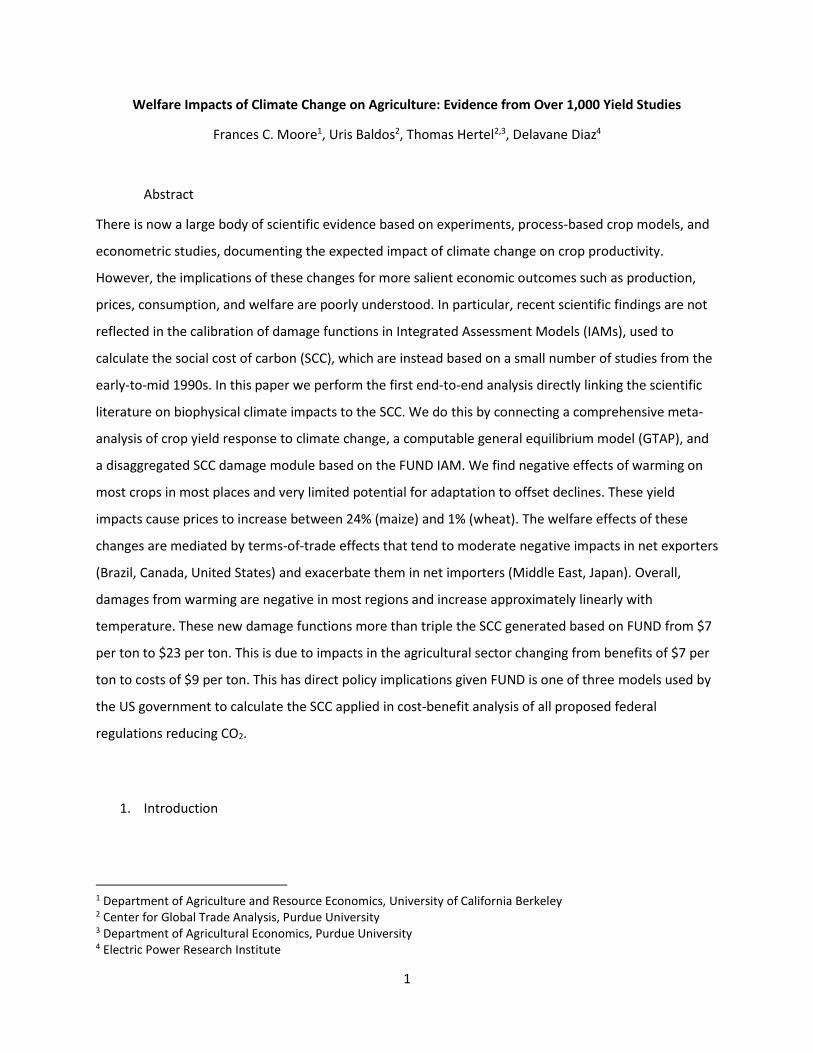
Welfare Impacts of Climate Change on Agriculture: Evidence from Over 1,000 Yield Studies

Frances C. Moore1, Uris Baldos2, Thomas Hertel2,3, Delavane Diaz4

Abstract

There is now a large body of scientific evidence based on experiments, process-based crop models, and

econometric studies, documenting the expected impact of climate change on crop productivity.

However, the implications of these changes for more salient economic outcomes such as production,

prices, consumption, and welfare are poorly understood. In particular, recent scientific findings are not

reflected in the calibration of damage functions in Integrated Assessment Models (IAMs), used to

calculate the social cost of carbon (SCC), which are instead based on a small number of studies from the

early-to-mid 1990s. In this paper we perform the first end-to-end analysis directly linking the scientific

literature on biophysical climate impacts to the SCC. We do this by connecting a comprehensive meta-

analysis of crop yield response to climate change, a computable general equilibrium model (GTAP), and

a disaggregated SCC damage module based on the FUND IAM. We find negative effects of warming on

most crops in most places and very limited potential for adaptation to offset declines. These yield

impacts cause prices to increase between 24% (maize) and 1% (wheat). The welfare effects of these

changes are mediated by terms-of-trade effects that tend to moderate negative impacts in net exporters

(Brazil, Canada, United States) and exacerbate them in net importers (Middle East, Japan). Overall,

damages from warming are negative in most regions and increase approximately linearly with

temperature. These new damage functions more than triple the SCC generated based on FUND from $7

per ton to $23 per ton. This is due to impacts in the agricultural sector changing from benefits of $7 per

ton to costs of $9 per ton. This has direct policy implications given FUND is one of three models used by

the US government to calculate the SCC applied in cost-benefit analysis of all proposed federal

regulations reducing CO2.

1. Introduction

1 Department of Agriculture and Resource Economics, University of California Berkeley 2 Center for Global Trade Analysis, Purdue University 3 Department of Agricultural Economics, Purdue University 4 Electric Power Research Institute

2

The economic damages associated with climate change will occur in many sectors and will vary widely in

both space and time. Though quantifying these damages is inherently challenging, it is a critical policy-

relevant question because these damages determine the social cost of carbon (SCC) and therefore

optimal rates of global greenhouse gas mitigation. The US government currently applies a SCC of $36 per

ton CO2, derived from three integrated assessment models (IAMs), to value the climate benefits of all

proposed federal regulations reducing CO2 (IAWG, 2015). However, the damage functions in these IAMs

have been the subject of much recent attention and scrutiny. In particular, several key limitations have

been widely noted: 1) the underlying studies used for calibration are outdated, 2) they lack rigorous

empirical content, 3) the coverage of key impact sectors is incomplete (Burke et al., 2016; Revesz et al.,

2014).

In this paper we focus specifically on agriculture, an impact sector that is highly exposed to climate

change and therefore is often a large component of total climate impacts. Understanding the economic

implications of climate impacts on agriculture is important both for sector-specific damages (e.g. FUND)

and for informing aggregate damage functions derived from bottom-up sector-specific studies (e.g.

DICE). Agriculture is also a sector in which the biophysical impacts of climate change have been

extensively studied and for which a large and robust body of evidence now exists (Porter et al., 2014).

Despite the importance of the sector and the large scientific literature on climate change impacts on

yields, relatively few studies have examined the implications for economically-relevant variables such as

prices, consumption, food-security, and welfare. Perhaps because of this, the empirical basis for IAM

damage functions comes almost entirely from the early- or mid-1990s (Fischer, Frohberg, Parry, &

Rosenzweig, 1996; Kane, Reilly, & Tobey, 1992; Morita et al., 1994; Reilly, Hohnmann, & Kane, 1994;

Tsigas, Frisvold, & Kuhn, 1996) meaning they are not informed by important scientific developments

over the last two decades including the use of open-air experimental plots to quantify the effect of CO2

fertilization (Long, Ainsworth, Leakey, Nösberger, & Ort, 2006) and the use of econometric methods to

quantify the effect of temperature and rainfall changes on yields (e.g. Lobell & Asner, 2003; Schlenker &

Roberts, 2009).

Modeling the macro-economic consequences of yield shocks is important for understanding the welfare

consequences of climate change impacts on agriculture for two reasons. Firstly, multiple margins of

3

agronomic and economic adaptation exist in agriculture: farmers will be able to adjust how they grow a

particular crop, the location and timing of crop growth will shift in response to climate change impacts,

trade in agricultural commodities will adjust and, finally, consumers will be able to substitute between

goods. Each of these adaptive responses will mediate the impacts of biophysical yield shocks on

economic welfare. Secondly, climate change impacts will vary by crop and by region, changing the

comparative advantage of countries, thereby creating winners and losers in global agricultural markets.

A few more recent studies have quantified the economic implications of climate-induced yield changes,

though we believe none have explicitly developed a new sectoral damage function for use in IAMs. The

Agricultural Model Inter-Comparison Project (AgMIP) has used both partial- and general-equilibrium

models to examine the economic implications of climate-induced yield shocks determined by a number

of process-based crop models participating in the project (Nelson et al., 2014). Although this study does

not report welfare changes, the analysis of multiple model outputs does show the importance of

economic adaptations in mediating biophysical yield impacts, particularly adjustment of crop areas.

Constinot, Donaldson and Smith (2014) use a single crop model to examine the effect of changing yield

potential on agricultural trade and output for 10 crops under the a high-emissions, business-as-usual

scenario. They show average global welfare changes of 14% of agricultural output and find that

adjustment of growing areas rather than trade is the most critical adaptation. Indeed, welfare impacts

are three times larger if growing areas remain fixed but only very slightly larger if trade patterns are

fixed. Hertel, Burke and Lobell (2010) use the Global Trade Analysis Project (GTAP) model to examine

the implications of climate-change induced yield changes on prices and food security. They find

heterogeneous effects across different population segments and large distributional changes for the

poorest households by 2030 under the worst-case yield scenarios.

This study contributes to the existing literature in several ways. Firstly, in contrast to previous work that

has used only one crop model (Costinot et al., 2014) or only process-based crop models (Rosenzweig et

al., 2014) we base our study on a current and comprehensive review of the scientific literature on crop-

response to temperature and CO2 fertilization, incorporating both process-based and empirical studies,

performed for the IPCC 5th Assessment Report (Challinor et al., 2014; Porter et al., 2014). Secondly this is

the first study in any sector (that we know of) that has produced an end-to-end analysis linking the

4

scientific literature on the biophysical impacts of climate change to the SCC. As such, this paper provides

an example of the type of work that will be necessary in the future if IAM damage functions are to have

an up-to-date and transparent foundation. Finally we perform a sensitivity analysis to compare multiple

margins of adaptation, both agronomic and economic, and therefore contribute to a growing literature

estimating the importance of adaptation in various sectors in determining climate change impacts (M. B.

Burke & Emerick, 2015; Moore & Lobell, 2014).

2. Methods

Our approach relies on three linked sets of analysis: a meta-analysis of the scientific literature to

determine the response of crop yields to temperature and atmospheric CO2 concentration; a

computable general equilibrium model to determine the effects of yield changes on economic

outcomes; and a disaggregated SCC damage module based on the Climate Framework for Uncertainty,

Negotiation, and Distribution (FUND) IAM to determine the implications of this new damage function on

the SCC (Anthoff & Tol, 2014; Diaz, 2014). We focus on the climate change impacts of four major crops –

maize, wheat, rice, and soybeans. The bulk of the scientific literature on yield response to temperature

focuses on these crops, which collectively account for approximately 20% of the value of global

agricultural production, 65% of harvested crop area, and just under 50% of calories consumed (FAO,

2016).

2.1 Yield Response to Temperature Change

The yield-temperature response functions used in this paper are derived from a database of studies

estimating the climate change impact on yield compiled for the IPCC 5th Assessment Report (Porter et

al., 2014), also described in a meta-analysis by Challinor et al. (2014). This database contains over 1700

point estimates of the impacts of changes in temperature, rainfall, and CO2 concentrations on the yield

of 17 different crops compiled from 94 different studies. These studies include a wide range of process-

based crop models as well as empirical papers, were published between the late 1990s and 2012, and

vary substantially in the geographic regions they examine as well as the extent to which they include on-

farm adaptations. For the four crops studied as part of this analysis, the database contains 1010

observations (344, 258, 336, and 92, for maize, rice, wheat and soybeans respectively) from 94 different

studies (many studies report multiple yield changes either for different crops, different levels of

5

temperature change, or different assumptions about adaptation). For maize and wheat the observations

are sufficient to estimate separate response functions for temperate and tropical regions. For rice and

soy we estimate a single response function for each crop.

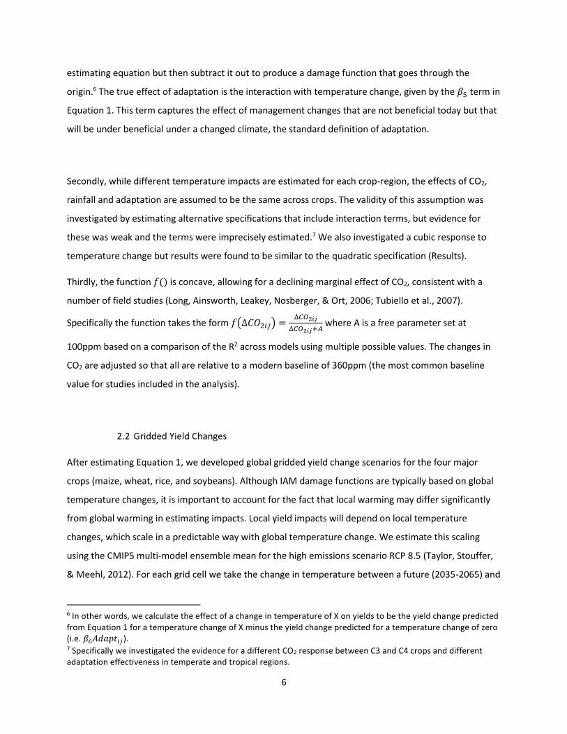
The response functions are jointly estimated from the point-estimates in the database using a multi-

variate regression:

∆𝑌𝑖𝑗 = 𝛽1𝑗∆𝑇𝑖𝑗 ∗ 𝐶𝑟𝑜𝑝𝑅𝑒𝑔𝑖𝑜𝑛𝑗 + 𝛽2𝑗∆𝑇𝑖𝑗2 ∗ 𝐶𝑟𝑜𝑝𝑅𝑒𝑔𝑖𝑜𝑛𝑗 + 𝛽3𝑓(∆𝐶𝑂2𝑖𝑗) + 𝛽4∆𝑃𝑖𝑗 + 𝛽5∆𝑇𝑖𝑗 ∗ 𝐴𝑑𝑎𝑝𝑡𝑖𝑗 +

𝛽6𝐴𝑑𝑎𝑝𝑡𝑖𝑗 + 휀𝑖𝑗 (1)

Where ∆𝑌𝑖𝑗 is the change in yield from point-estimate i for crop-region j (in %)5. ∆𝑇𝑖𝑗, ∆𝐶𝑂2𝑖𝑗 and ∆𝑃𝑖𝑗

are the changes in temperature (in degrees C), CO2 concentration (in parts per million (ppm)) and rainfall

(in percent) for point-estimate ij, and 𝐴𝑑𝑎𝑝𝑡𝑖𝑗 is a dummy variable indicating whether the point-

estimate includes any on-farm adaptation. 𝐶𝑟𝑜𝑝𝑅𝑒𝑔𝑖𝑜𝑛𝑗 is a dummy variable taking the value 1 if the

point-estimate is in crop-region j and 0 otherwise. Equation 1 is estimated using an ordinary least

squares regression. Uncertainty in the parameters is estimated through 750 block bootstraps, with

blocks defined at the study level, allowing for possible auto-correlation between point-estimates from

the same study. Error bars reported throughout the paper are based on the 2.5th and 97.5th quantiles of

the bootstrapped distribution.

There are a number of important things to note about this specification. Firstly there is no intercept

term, thereby forcing response functions without adaptation through the origin. This is consistent with

the expected functional form of a damage function, which should have no impacts if there are no

changes in climate variables. However, we include an intercept for studies that do include adaptation.

This is prompted by the observation that in many studies, adaptation is represented by changing

management practices that would improve yields even in the current climate, such as increasing

fertilizer or irrigation inputs (Lobell, 2014). Failing to include an adaptation intercept in this context will

lead to an over-estimation of the potential of the adaptation actions included in these studies to reduce

the negative impacts of a warming climate. We therefore include an adaptation intercept in the

5 As described in the previous paragraph, there are 6 crop-regions: temperate maize, tropical maize, temperate wheat, tropical wheat, rice, and soybeans.

6

estimating equation but then subtract it out to produce a damage function that goes through the

origin.6 The true effect of adaptation is the interaction with temperature change, given by the 𝛽5 term in

Equation 1. This term captures the effect of management changes that are not beneficial today but that

will be under beneficial under a changed climate, the standard definition of adaptation.

Secondly, while different temperature impacts are estimated for each crop-region, the effects of CO2,

rainfall and adaptation are assumed to be the same across crops. The validity of this assumption was

investigated by estimating alternative specifications that include interaction terms, but evidence for

these was weak and the terms were imprecisely estimated.7 We also investigated a cubic response to

temperature change but results were found to be similar to the quadratic specification (Results).

Thirdly, the function 𝑓() is concave, allowing for a declining marginal effect of CO2, consistent with a

number of field studies (Long, Ainsworth, Leakey, Nosberger, & Ort, 2006; Tubiello et al., 2007).

Specifically the function takes the form 𝑓(∆𝐶𝑂2𝑖𝑗) =∆𝐶𝑂2𝑖𝑗

∆𝐶𝑂2𝑖𝑗+𝐴 where A is a free parameter set at

100ppm based on a comparison of the R2 across models using multiple possible values. The changes in

CO2 are adjusted so that all are relative to a modern baseline of 360ppm (the most common baseline

value for studies included in the analysis).

2.2 Gridded Yield Changes

After estimating Equation 1, we developed global gridded yield change scenarios for the four major

crops (maize, wheat, rice, and soybeans). Although IAM damage functions are typically based on global

temperature changes, it is important to account for the fact that local warming may differ significantly

from global warming in estimating impacts. Local yield impacts will depend on local temperature

changes, which scale in a predictable way with global temperature change. We estimate this scaling

using the CMIP5 multi-model ensemble mean for the high emissions scenario RCP 8.5 (Taylor, Stouffer,

& Meehl, 2012). For each grid cell we take the change in temperature between a future (2035-2065) and

6 In other words, we calculate the effect of a change in temperature of X on yields to be the yield change predicted from Equation 1 for a temperature change of X minus the yield change predicted for a temperature change of zero (i.e. 𝛽6𝐴𝑑𝑎𝑝𝑡𝑖𝑗). 7 Specifically we investigated the evidence for a different CO2 response between C3 and C4 crops and different adaptation effectiveness in temperate and tropical regions.

7

baseline (1861-1900) period and divide by the mean global warming over this time period, giving the

pattern scaling relationship between global and local temperature change for each grid cell (Figure A1).

For a given increase in global mean temperature, warming is larger over land than over the ocean and at

high latitudes compared to the tropics.

These gridded temperature changes are combined with the yield-temperature response function

estimated using Equation 1 and a classification of each grid square into temperate, tropical or boreal

agro-ecological zone. The yield change in the boreal region is assumed to be zero. This is a known

weakness of this analysis but is necessary to avoid unsupported extrapolation beyond the evidence of

the yield studies included in our meta-analysis, none of which examine changes in the boreal zones. For

maize and wheat, different response functions are used in the tropical and temperate zones while for

rice and soybeans the same response function is used in both. We calculate yield changes for global

temperature increases of 1, 2, 3, 4, and 5 degrees Celsius. For each scenario this gives us 15 gridded

yield products (3 quantiles of the parameter distribution for each of 5 temperature changes). Most of

the results that follow are based on our preferred scenario that includes on-farm adaptation and the

CO2 fertilization effect for C3 crops but not C4 (broadly consistent with experimental field trials (Long et

al., 2006)). In our sensitivity analysis we also report results that include CO2 fertilization for all crops,

exclude CO2 fertilization for all crops, and that exclude on-farm adaptation. For scenarios that include

the CO2 fertilization effect, CO2 concentrations are determined based on a fitted quadratic relationship

between global temperature change and CO2 concentrations from the RCP 8.5 CMIP5 multi-model

ensemble mean.

2.3 GTAP Model and Scenario Analysis

To understand the economic implications of warming-induced yield shocks, we use the Global Trade

Analysis Project (GTAP) general equilibrium model and its accompanying database (T. W. Hertel, 1997;

Narayanan, Aguiar, & McDougall, 2015). GTAP is a widely-used, comparative static general equilibrium

model which exhaustively tracks bilateral trade flows between all countries in the world, and explicitly

models the consumption and production for all commodities of each national economy. Producers are

assumed to maximize profits, while consumers maximize utility. Factor market clearing requires that

supply equal demand for agricultural and non-agricultural skilled and unskilled labor and capital, natural

8

resources and agricultural land, and adjustments in each of these markets in response to the climate

change shocks determines the resulting wage and rental rate impacts. The model has been validated

with respect to its performance in predicting the price impacts of exogenous supply side shocks, such as

those that might result from global climate change (Valenzuela, Hertel, Keeney, & Reimer, 2007).

GTAP captures a number of dimensions important for determining the welfare implications of climate

change impacts on agriculture.. These include the shifting of land area between crops, potential

intensification of production, shifting of consumption between commodities and sources of goods, and

finally, the adjustment of global trade patterns. For the purposes of this study, GTAP is run with 140

regions and 14 commodities which place an emphasis on the agricultural sector. Wheat and rice are

modeled as individual sectors within each region. Maize is part of the coarse grains sector and soybeans

as part of the oilseeds sector. Impacts in these sectors are scaled downwards based on the importance

of maize and soybeans for production. Yields of crops not covered in the meta-analysis (coarse grains

nec., oilseeds nec, sugarcane, cotton and fruits and vegetables) are not altered. Absent some kind of

normalization, this will lead to an underestimate of potential climate impacts. Therefore, in the results

that follow, welfare changes are normalized by the value of production only of the crops covered in the

meta-analysis. More details on the structure of GTAP are given in the Appendix.Global and regional

welfare changes are measured in terms of Equivalent Variation and are decomposed into three

components following Hertel and Randhir (2000). Firstly there is the direct effect of climate change on

agricultural productivity, modeled as a Hicks-neutral technical change in crop production. This supply

shock can be multiplied by the value of output at producer prices to evaluate its contribution to the

regional welfare change. Secondly there are allocative efficiency effects resulting from the interaction of

changing production, consumption and trade patterns within a second-best policy setting (production

subsidies or taxes, consumption interventions, export subsidies or taxes and import tariffs). These can

be favorable (e.g., when climate change encourages more importation of a taxed product) or

unfavorable (e.g., when climate change encourages more production of subsidized output). Finally there

are regional terms of trade effects which depend on the prices of region’s exports, relative to its

imports.

2.4 Implications for the SCC

9

Results of the economic modeling are used to create damage functions that relate changes in economic

welfare (measured as % of the agricultural sector sector) with temperature change. GTAP results are

aggregated from the country level to the 16 FUND regions. Damage functions are based on a linear

interpolation between the point estimates of welfare changes of 1, 2, and 3° of warming and then a

linear extrapolation beyond 3°.

These agricultural damage functions are then incorporated into a sectorally- and regionally-

disaggregated SCC damage module based on the FUND model, keeping the rest of the impact sectors

unchanged (Anthoff & Tol, 2014; Diaz, 2014). The SCC is calculated by adding a 1 Gt pulse of CO2

emissions to the BAU reference emissions path in 2020 and comparing the time path of damages along

the perturbed pathway to the reference case. Then these incremental damages (or benefits) are

discounted back to 2020 at a 3% discount rate and normalized by the CO2 pulse volume to give the SCC.

As the SCC is additive, it can be decomposed by sector and region, allowing a detailed comparison of the

regional impacts in agriculture between FUND and the revised regional damage functions.

3 Results

3.1 Yield – Temperature Response Function

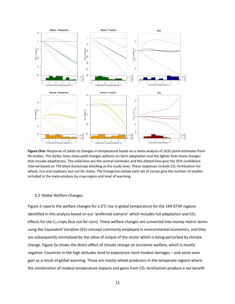
Figure 1 gives the response of yields to temperature estimated from the meta-analysis of yield studies

for the preferred scenario that includes CO2 fertilization for the C3 crops but excludes it for maize (a C4

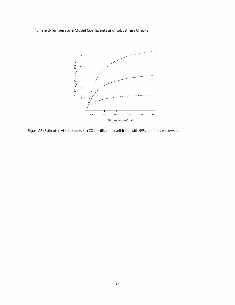
crop). Figure A3 gives the estimated response to CO2 which shows a benefit of 12.3% for a doubling of

CO2. This is close to values obtained for C3 crops from experimental field plots grown under elevated CO2

conditions, which range from 12% for rice to 14% for soybeans (Long et al., 2006). However, similar

experiments do not find any benefits from higher CO2 concentrations for maize, consistent with the

observation that the C4 photosynthesis pathway is saturated with respect to CO2 at current atmospheric

concentrations (Leakey, 2009; Leakey et al., 2006). This means that maize yields are unlikely to benefit

from higher CO2 concentrations, except under drought conditions, which is why we do not include maize

CO2 fertilization in our preferred scenario (though do include it as part of our sensitivity analysis).

10

For crops where responses in tropical and temperate areas could be distinguished, both show worse

effects in the warmer tropics than in cooler temperate areas. This is particularly striking for wheat in the

tropics which shows yield declines of over 40% for a warming of 5 degrees, even including on-farm

adaptation and CO2 fertilization. For temperature changes below 2 degrees, the combination of large

positive effects from CO2 fertilization and small negative impacts of warming result in positive effects on

wheat and rice yields. At higher temperatures, the CO2 effect saturates and the damaging effects of

warming dominate meaning almost all crops show negative impacts at high levels of warming.

Uncertainty bounds are large, particularly for soybeans, for which very few studies exist at high

temperatures.

One striking aspect of Figure 1 is the similarity between the curves that include and exclude on-farm

adaptation. The estimated effect of adaptation (𝛽5 in Equation One) is positive (0.13 pp per degree

warming) but is small and not significantly different from zero. Studies that include adaptive

management options do, on average, have higher yields than those that don’t, but this mostly has the

effect of shifting up the yield-temperature response curve, rather than actually changing its shape. This

means the negative impacts of warming are similar both with and without adaptation, resulting in the

very similar damage functions shown in Figure 1. Table A1 gives the full set of coefficients and standard

errors, as well as several robustness checks.

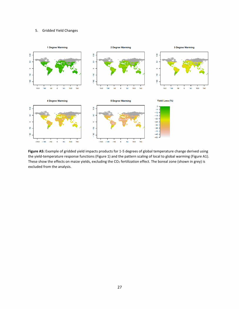
Gridded yield changes for maize for global warming of 1-5 degrees are shown in Figure A5 as an example

of the gridded outputs used as inputs to the GTAP model. For a given level of global warming, local

effects on yield vary depending on the pattern scaling between local and global temperature change

(Figure A1) and (for maize and wheat) whether the region is in the temperate or tropical zone. Impacts

are larger inland and at higher latitudes (due to larger local warming) and in the tropics compared to the

temperate zone (due to a steeper yield response function). The boreal zone is excluded from the

analysis due to a lack of studies examining the effects of yield change in these areas.

11

Figure One: Response of yields to changes in temperature based on a meta-analysis of 1010 point-estimates from

94 studies. The darker lines show yield changes without on-farm adaptation and the lighter lines show changes

that include adaptations. The solid lines are the central estimates and the dotted lines give the 95% confidence

interval based on 750 block bootstraps blocking at the study level. These responses include CO2 fertilization for

wheat, rice and soybeans but not for maize. The histograms below each set of curves give the number of studies

included in the meta-analysis by crop-region and level of warming.

3.2 Global Welfare Changes

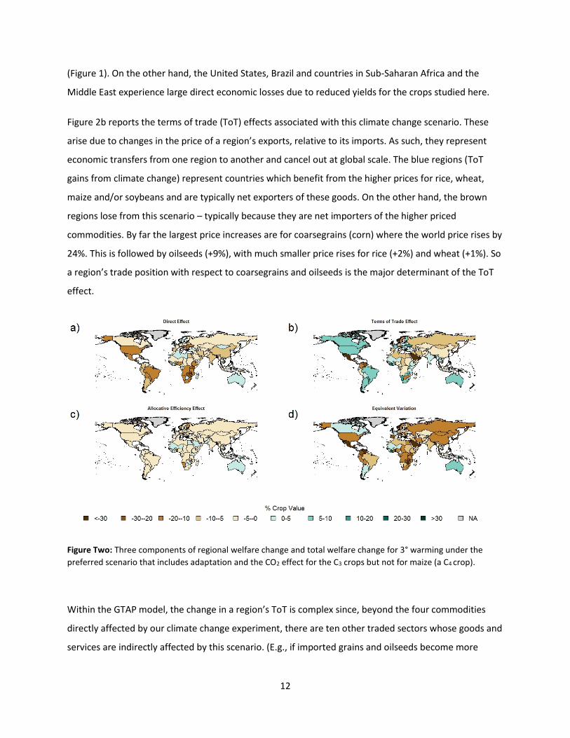
Figure 2 reports the welfare changes for a 3°C rise in global temperature for the 140 GTAP regions

identified in this analysis based on our ‘preferred scenario’ which includes full adaptation and CO2

effects for the C3 crops (but not for corn). These welfare changes are converted into money metric terms

using the Equivalent Variation (EV) concept commonly employed in environmental economics, and they

are subsequently normalized by the value of output of the sector which is being perturbed by climate

change. Figure 2a shows the direct effect of climate change on economic welfare, which is mostly

negative. Countries in the high latitudes tend to experience more modest damages – and some even

gain as a result of global warming. These are mostly wheat producers in the temperate regions where

the combination of modest temperature impacts and gains from CO2 fertilization produce a net benefit

12

(Figure 1). On the other hand, the United States, Brazil and countries in Sub-Saharan Africa and the

Middle East experience large direct economic losses due to reduced yields for the crops studied here.

Figure 2b reports the terms of trade (ToT) effects associated with this climate change scenario. These

arise due to changes in the price of a region’s exports, relative to its imports. As such, they represent

economic transfers from one region to another and cancel out at global scale. The blue regions (ToT

gains from climate change) represent countries which benefit from the higher prices for rice, wheat,

maize and/or soybeans and are typically net exporters of these goods. On the other hand, the brown

regions lose from this scenario – typically because they are net importers of the higher priced

commodities. By far the largest price increases are for coarsegrains (corn) where the world price rises by

24%. This is followed by oilseeds (+9%), with much smaller price rises for rice (+2%) and wheat (+1%). So

a region’s trade position with respect to coarsegrains and oilseeds is the major determinant of the ToT

effect.

Figure Two: Three components of regional welfare change and total welfare change for 3° warming under the

preferred scenario that includes adaptation and the CO2 effect for the C3 crops but not for maize (a C4 crop).

Within the GTAP model, the change in a region’s ToT is complex since, beyond the four commodities

directly affected by our climate change experiment, there are ten other traded sectors whose goods and

services are indirectly affected by this scenario. (E.g., if imported grains and oilseeds become more

13

expensive, the country must export more of other goods and services, the price of which will fall as a

result.) In addition, since global commodity markets are imperfectly integrated, the bilateral patterns of

trade also play a role – it matters whom you are trading with. However, the broad outline of terms of

trade impacts in Figure 2 are as expected, with the major exporters Canada, USA, Brazil, Argentina,

Paraguay, South Africa and Australia being amongst the largest winners, while Mexico, Colombia,

Venezuela, North Africa, Saudi Arabia, East Asia and Russia being significant losers from the higher price

imports.

The third contributor to the aggregate national welfare effect of climate change is the so-called

‘allocative efficiency’ effect which tracks how climate change interacts with existing policies (Figure 2c).

If current economic policies were perfectly neutral in their effect (i.e., economically efficient) there

would be no room for allocative efficiency changes from climate impacts. However, this is hardly the

case, and some of the largest distortions to economic activity are in the agricultural sector. China, for

example, has recently started spending a large amount of money on subsidies for its agricultural sector

(OECD, 2016). In our preferred experiment, there is a very substantial negative productivity shock to the

coarse grains sector in China due to the adverse impact of climate change on corn. As a consequence,

more land, labor and capital are drawn into this sector, in an effort to maintain output levels. Each unit

of these endowments brings with it additional subsidies, thereby reducing overall efficiency in the

Chinese economy. Indeed, China’s allocative efficiency losses account for 36% of the global efficiency

losses, which total $11.3 billion. However, this global allocative effect is much less important than the

direct effect (a loss of $73.2 billion), and, at the country level, the allocative effect is also dominated by

the terms of trade effect in most regions.

When the direct, terms of trade, and allocative effects are summed, we obtain the total welfare effect

shown in Figure 2d. The largest losses are in those regions where both the direct and the terms of trade

effects are negative. In percentage terms, regions with relatively small staple grains and oilseeds sectors

also show larger losses, since the aggregate loss is divided by a smaller number. Thus Mexico, most of

Central America, Venezuela, Saudi Arabia, and a number of other middle eastern countries all show

welfare losses in excess of 30% of the value of output in these sectors. In contrast, countries with

positive direct and terms of trade effects show significant gains under the ‘preferred’ climate change

scenario. Here, New Zealand and Australia stand out, among other countries.

14

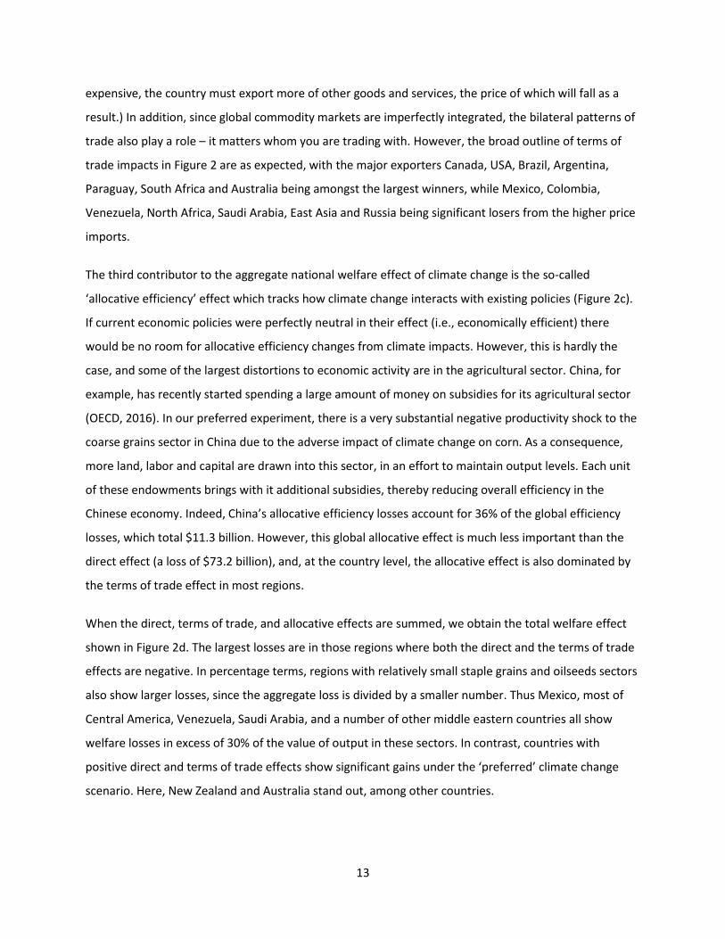
Figure Three: Agricultural sector damage functions for the 16 FUND regions. Solid lines show the damages

estimated in this study with error bars based on the 95% confidence intervals of the yield-temperature response

function. Dashed lines show the implied damage functions for a FUND-based SCC damage module. Welfare

changes are given as % of the agricultural sector.

3.3 Implications for the Social Cost of Carbon

Figure 3 shows the total welfare effects aggregated from the 140 GTAP regions to the 16 regions used in

FUND for warming of 1,2 and 3°C. These regional agricultural sector damage functions are compared to

the implied damage functions from a FUND-based SCC damage module under a BAU scenario in 2100.

Important differences are immediately apparent. FUND includes fairly large benefits from CO2

fertilization (positive effect of between 3 and 17% for a doubling of CO2 depending on the region) as well

as positive effects of temperature levels for moderate amounts of warming (Anthoff & Tol, 2014). The

combined effect of these is to produce positive impacts in all regions for up to 5°C of warming. In

contrast, results from this study show negative effects in almost all regions even for only moderate

warming. In most cases, FUND-based damages are at the very top end of the 95% confidence intervals

based on uncertainty in our estimates of yield response to temperature changes (Figure 1). In several

cases (Central and Easter Europe, China, Small Island States, and the USA), the FUND damage function

15

lies outside the confidence intervals estimated in this study. Only for the Australia and New Zealand

region is there a close match between existing FUND damages and our estimates.

These differences in the agricultural sector damage functions have large implications for the social cost

of carbon (SCC). Although FUND includes over 200 damage functions (14 sectors in each of 16 regions),

the parameterization is such that only a few sectors (namely heating costs, cooling costs, and the

agricultural sector) have substantial implications for the SCC (Diaz, 2014). Replacing the existing

agricultural damage functions with those estimated in this study increases the agriculture sector’s

component of the global SCC from a benefit of $7 per ton to a damage of $9 per ton (Figure 3, calculated

using a 3% discount rate). Because the non-agriculture impact sectors constitute an SCC of $14, these

new agriculture damage functions drive the total SCC up from $7 per ton CO2 to $23 per ton.

Figure Four: Decomposition of the SCC from FUND using the existing agricultural-sector damage functions and the

updated agricultural damage functions presented in this study. Total damages (right-hand bars) are the sum of

non-agricultural sector damages (left-hand bar) and the agricultural sector damages. Agricultural sector damages

are decomposed into contributions from each of the 16 FUND regions. Negative values indicate a benefit from CO2

emissions. All SCC values are calculated using a 3% discount rate.

16

4 Discussion and Conclusions

There is now a large literature on the consequences of greenhouse gas emissions for crop yields,

including process-based, empirical, and experimental studies, which has lead to an increasingly

sophisticated scientific understanding of the risks climate change poses to crop productivity. However,

there is also a clear gap in our knowledge regarding how these changes will affect less immediate but

more salient economic variables such as production, prices, consumption, and welfare. Partly because of

this gap, damage functions in IAMs remain calibrated to studies dating back more than two decades.

In this study we build on a comprehensive and complete review of the scientific body of evidence

regarding crop response to climate change (Challinor et al., 2014; Porter et al., 2014). Matching findings

of previous work, our meta-analysis of these studies shows negative impacts at high temperatures, even

when CO2 fertilization is included. The potential for agronomic adaptation options to mitigate the

negative consequences of high temperatures appears to be limited. Our results suggest that many of the

adaptations commonly-discussed in the literature would improve yields in the current and future

climate, but will not necessarily reduce the negative impacts of warming.

The GTAP results highlight the importance of global trade for determining the economic consequences

of yield shocks. The direct effects of climate change on yields are large and negative in most regions,

leading to large impacts on world prices. These price changes, in turn, give rise to terms-of-trade effects

wherein the welfare of a given country is affected by a change in the price of goods it sells (exports),

relative to the price of purchases (imports). In many areas (Mexico and the Middle East for example),

the terms of trade effect of climate change greatly exacerbate negative climate shocks, whereas in some

areas (Brazil, United States) they mitigate the welfare consequences of adverse yield changes. Indeed, in

the case of Canada, the terms of trade change converts a negative direct yield effect into an overall

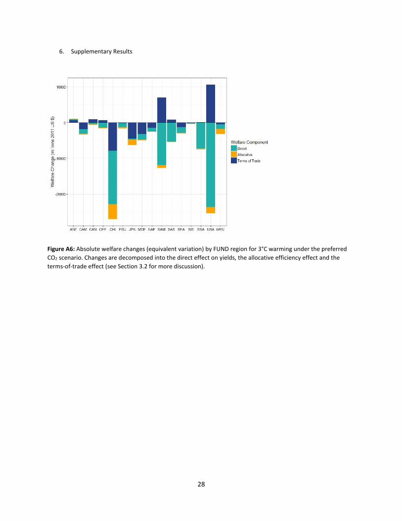
welfare gain. Figure A6 shows the importance of each component of the welfare change. In several

regions, including the Japan and Korea, Central America, and the Middle East, terms-of-trade effects

constitute well over half of total welfare impacts.

The economic damage to agriculture estimated in this study is significantly different from that currently

represented in the FUND model. The FUND damage functions imply positive effects of warming at low

temperatures, largely driven by beneficial effects from CO2 fertilization. The magnitude of CO2

fertilization that we estimate seems to be similar to that currently used in FUND. The differing impact

estimates are instead largely attributable to the negative impacts of temperature change on most crops,

17

even for low levels of warming. This difference reflects a changing scientific understanding of the

impacts of high temperatures on crop yields since FUND was calibrated in the mid-1990s and

demonstrates the importance of routine, frequent, and transparent updates to IAM damage functions.

Because agriculture is one of few sectors that has a materially affects the SCC in FUND, incorporating

our new damage functions in a disaggregated damage module has a substantial effect on the SCC,

raising it from $7 per ton CO2 to $23 using a 3% discount rate. Given that FUND is one of only three IAMs

currently used by the US government to determine the SCC applied in cost-benefit analyses of climate-

relevant policies, this difference has significant policy implications. Of the three models used, FUND

consistently reports the lowest SCC, a result driven in large part by benefits in its agricultural sector

(Diaz, 2014; IAWG, 2013). Given these benefits are no longer consistent with scientific understanding of

climate change impacts, an update to damage functions in the agricultural sector to bring them more in

line with results reported here would seem to be important from both a scientific and policy

perspective.

There are several important caveats to the results presented here that should be noted. There are two

reasons in particular why our results might be overly pessimistic. Firstly our method for aggregating the

scientific literature on yield response to temperature changes means we do not capture potential yield

gains at high latitudes. It may be that very cold areas which are not currently suitable for crops will

benefit from warmer temperatures in ways not captured in the studies we use that are based in

temperate and tropical latitudes. To the extent agriculture will be able to shift locations to take

advantage of these gains, welfare impacts will be lower than those estimated here. Secondly, to obtain

damages for the whole agricultural sector, we are required to extrapolate from the four crops studied

here (wheat, rice, maize and soybeans). We do this by first normalizing welfare changes by the value of

crops affected and then applying these normalized results to the whole sector, effectively assuming that

products not explicitly studied will be affected in similar ways to those included. While these four crops

do account for 50% of direct caloric consumption and are also important for livestock fodder (FAO,

2016), it is possible that direct effects for some products (particularly sugarcane, cotton, and livestock)

might well be smaller than assumed here. Future research should aim to broaden the scientific basis for

this type of climate impact analysis in agriculture.

References

18

Anthoff, D., & Tol, R. S. J. (2014). FUND v3.9 Scientific Documentation. Retrieved April 12, 2016, from http://www.fund-model.org/versions

Brockmeier, M. (2001). A Graphical Exposition of the GTAP Model (GTAP Technical Paper No. 8). Purdue University.

Burke, M. B., & Emerick, K. (2015). Adaptation to Climate Change: Evidence from U.S. Agriculture. Retrieved from http://web.stanford.edu/~mburke/papers/Burke_Emerick_2015.pdf

Burke, M., Craxton, M., Kolstad, C. D., Onda, C., Allcott, H., Baker, E., … Tol, R. S. J. (2016). Opportunities for advances in climate change economics. Science, 352(6283), 292–293. Retrieved from http://science.sciencemag.org/content/352/6283/292.abstract

Challinor, A. J., Watson, J., Lobell, D. B., Howden, S. M., Smith, D. R., & Chhetri, N. (2014). A meta-analysis of crop yield under climate change and adaptation. Nature Climate Change, 4(4), 287–291. http://doi.org/10.1038/nclimate2153

Costinot, A., Donaldson, D., & Smith, C. B. (2014). Evolving Comparative Advantage and the Impact of Climate Change in Agricultural Markets: Evidence from 1.7 Million Fields around the World. Retrieved from http://www.nber.org/papers/w20079

Diaz, D. B. (2014). Evaluating the Key Drivers of the US Government’s Social Cost of Carbon: A Model Diagnostic and Inter-Comparison Study of Climate Impacts in DICE, FUND, and PAGE.

FAO. (2016). FAOSTAT, V.3. Retrieved April 4, 2016, from faostat3.fao.org

Fischer, G., Frohberg, K., Parry, M. L., & Rosenzweig, C. (1996). Impacts of Potential Climate Change on Global and Regional Food Production and Vulnerability. In T. Downing (Ed.), Climate Change and World Food Security (pp. 115–159). Berlin: Springer-Verlag.

Hertel, T. W. (1997). Global Trade Analysis: Models and Applications. Cambridge, UK: Cambridge University Press.

Hertel, T. W., Burke, M. B., & Lobell, D. B. (2010). The poverty implications of climate-induced crop yield changes by 2030. Global Environmental Change, 20(4), 577–585. http://doi.org/10.1016/j.gloenvcha.2010.07.001

Hertel, T. W., & Randhir, T. O. (2000). Trade Liberalization as a Vehicle for Adapting to Global Warming. Agricultural and Resource Economics Review, 29(2), 159–172.

IAWG, U. (2013). Technical support document: Technical update of the social cost of carbon for regulatory impact analysis under executive order 12866, (November), 1–22.

Kane, S., Reilly, J., & Tobey, J. (1992). An Empirical Study of the Economic Effects of Climate Change on World Agriculture. Climatic Change, 21, 17–35.

Leakey, A. D. B. (2009). Rising atmospheric carbon dioxide concentration and the future of C4 crops for food and fuel. Proceedings. Biological Sciences / The Royal Society, 276(1666), 2333–43. http://doi.org/10.1098/rspb.2008.1517

Leakey, A. D. B., Uribelarrea, M., Ainsworth, E. A., Naidu, S. L., Rogers, A., Ort, D. R., & Long, S. P. (2006). Photosynthesis, productivity, and yield of maize are not affected by open-air elevation of CO2 concentration in the absence of drought. Plant Physiology, 140(2), 779–90. http://doi.org/10.1104/pp.105.073957

19

Lobell, D. (2014). Climate change adaptation in crop production : Beware of illusions. Global Food Security, 1–5. http://doi.org/10.1016/j.gfs.2014.05.002

Lobell, D. B., & Asner, G. P. (2003). Climate and Management Contributions to Recent Trends in U.S. Agricultural Yields. Science, 299, 1032.

Long, S. P., Ainsworth, E. a, Leakey, A. D. B., Nösberger, J., & Ort, D. R. (2006). Food for Thought: Lower-Than-Expected Crop Yield Stimulation with Rising CO2 Concentrations. Science, 312(5782), 1918–21. http://doi.org/10.1126/science.1114722

Long, S. P., Ainsworth, E. A., Leakey, A. D. B., Nosberger, J., & Ort, D. R. (2006). Food for Thought: Lower-Than-Expected Crop Yield Stimulation with Rising CO2 Concentrations. Science, 312, 1918–1921.

Mendelsohn, R., Morrison, W., Schlesinger, M. E., & Andronova, N. G. (2000). Country-Specific Market Impacts of Climate Change. Climatic Change, 45, 553–569.

Moore, F. C., & Lobell, D. B. (2014). The Adaptation Potential of European Agriculture in Response to Climate Change. Nature Climate Change, 4(7), 610–614.

Morita, T., Kainuma, M. L. T., Harasawa, H., Kai, K., Dong-Kun, L., & Matsuoka, Y. (1994). Asian-Pacific Integrated Model for Evaluating Policy Options to Reduce Greenhouse Gas Emissions and Global Warming Impacts. Tsukuba.

Narayanan, B., Aguiar, A., & McDougall, R. (2015). Global Trade, Assistance, and Production: The GTAP 9 Data Base. Purdue, IN: Center for Global Trade Analysis. Retrieved from http://www.gtap.agecon.purdue.edu/databases/v9/v9_doco.asp

Nelson, G. C., Valin, H., Sands, R. D., Havlík, P., Ahammad, H., Deryng, D., … Willenbockel, D. (2014). Climate change effects on agriculture: economic responses to biophysical shocks. Proceedings of the National Academy of Sciences of the United States of America, 111(9), 3274–9. http://doi.org/10.1073/pnas.1222465110

OECD. (2016). Producer and Consumer Support Estimates. Retrieved from http://www.oecd.org/tad/agricultural-policies/producerandconsumersupportestimatesdatabase.htm

Porter, J. R., Xie, L., Challinor, A. J., Cochrane, K., Howden, M., Iqbal, M. M., … Travasso, M. (2014). Chapter 7: Food Security and Food Production Systems. In Climate Change 2014: Impacts, Adaptation and Vulnerability. Working Group 2 Contribution to the IPCC 5th Assessment Report. Cambridge, UK: Cambridge University Press.

Reilly, J., Hohnmann, N., & Kane, S. (1994). Climate Change and Agricultural Trade: Who Benefits and Who Loses? Global Environmental Change, 4(1), 24–36.

Revesz, R., Arrow, K., Goulder, L., Kopp, R. E., Livermore, M., Oppenheimer, M., & Sterner, T. (2014). Improve Economic Models of Climate Change. Nature, 508, 173–175.

Rosenzweig, C., Elliott, J., Deryng, D., Ruane, A. C., Müller, C., Arneth, A., … Jones, J. W. (2014). Assessing agricultural risks of climate change in the 21st century in a global gridded crop model intercomparison. Proceedings of the National Academy of Sciences of the United States of America, 111(9), 3268–73. http://doi.org/10.1073/pnas.1222463110

Schlenker, W., & Roberts, D. L. (2009). Nonlinear Temperature Effects Indicate Severe Damages to U.S.

20

Corn Yields Under Climate Change. Proceedings of the National Academy of Sciences, 106(37), 15594–15598.

Taylor, K. E., Stouffer, R. J., & Meehl, G. A. (2012). An Overview of CMIP5 and the Experiment Design. Bulletin of the American Meteorological Society, 93, 485–498.

Tsigas, M. E., Frisvold, G. B., & Kuhn, B. (1996). Global Climate Change in Agriculture. In T. Hertel (Ed.), Global Trade Analysis: Modelling and Applications. Cambridge: Cambridge University Press.

Tubiello, F. N., Amthor, J. S., Boote, K. J., Donatelli, M., Easterling, W., Fischer, G., … Rosenzweig, C. (2007). Crop response to elevated CO 2 and world food supply A comment on “ Food for Thought . . . ” by Long et al ., Science 312 : 1918 – 1921 , 2006, 26, 215–223. http://doi.org/10.1016/j.eja.2006.10.002

Valenzuela, E., Hertel, T. W., Keeney, R., & Reimer, J. J. (2007). Assessing Global Computable General Equilibrium Model Validity Using Agricultural Price Volatility. American Journal of Agricultural Economics, 89(2), 383–397.

21

Appendix

1. Current Representation of Agricultural Damages in FUND

There are two published sources of agriculture damage functions, FUND and GIM (Anthoff & Tol, 2014;

Mendelsohn, Morrison, Schlesinger, & Andronova, 2000). We focus our comparison on FUND, which has

been in regular use for over 20 years and is a direct component of the USG SCC (IAWG 2010, 2013).

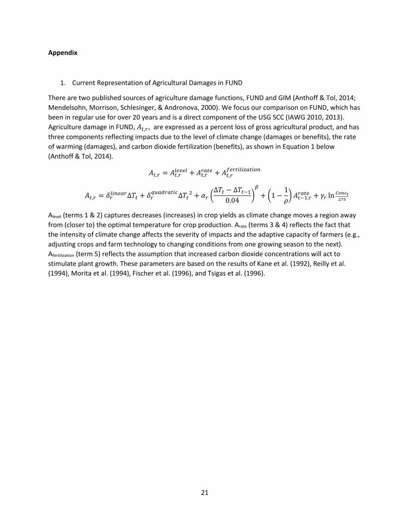
Agriculture damage in FUND, 𝐴𝑡,𝑟, are expressed as a percent loss of gross agricultural product, and has

three components reflecting impacts due to the level of climate change (damages or benefits), the rate

of warming (damages), and carbon dioxide fertilization (benefits), as shown in Equation 1 below

(Anthoff & Tol, 2014).

𝐴𝑡,𝑟 = 𝐴𝑡,𝑟𝑙𝑒𝑣𝑒𝑙 + 𝐴𝑡,𝑟

𝑟𝑎𝑡𝑒 + 𝐴𝑡,𝑟𝑓𝑒𝑟𝑡𝑖𝑙𝑖𝑧𝑎𝑡𝑖𝑜𝑛

𝐴𝑡,𝑟 = 𝛿𝑟𝑙𝑖𝑛𝑒𝑎𝑟Δ𝑇𝑡 + 𝛿𝑟

𝑞𝑢𝑎𝑑𝑟𝑎𝑡𝑖𝑐Δ𝑇𝑡

2 + 𝛼𝑟 (Δ𝑇𝑡 − Δ𝑇𝑡−1

0.04)

𝛽

+ (1 −1

𝜌) 𝐴𝑡−1,𝑟

𝑟𝑎𝑡𝑒 + 𝛾𝑟 ln 𝐶𝑜𝑛𝑐𝑡275

Alevel (terms 1 & 2) captures decreases (increases) in crop yields as climate change moves a region away

from (closer to) the optimal temperature for crop production. Arate (terms 3 & 4) reflects the fact that

the intensity of climate change affects the severity of impacts and the adaptive capacity of farmers (e.g.,

adjusting crops and farm technology to changing conditions from one growing season to the next).

Afertilization (term 5) reflects the assumption that increased carbon dioxide concentrations will act to

stimulate plant growth. These parameters are based on the results of Kane et al. (1992), Reilly et al.

(1994), Morita et al. (1994), Fischer et al. (1996), and Tsigas et al. (1996).

22

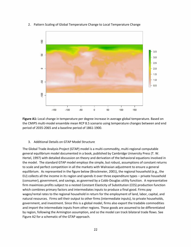
2. Pattern Scaling of Global Temperature Change to Local Temperature Change

Figure A1: Local change in temperature per degree increase in average global temperature. Based on

the CMIP5 multi-model ensemble mean RCP 8.5 scenario using temperature changes between and end

period of 2035-2065 and a baseline period of 1861-1900.

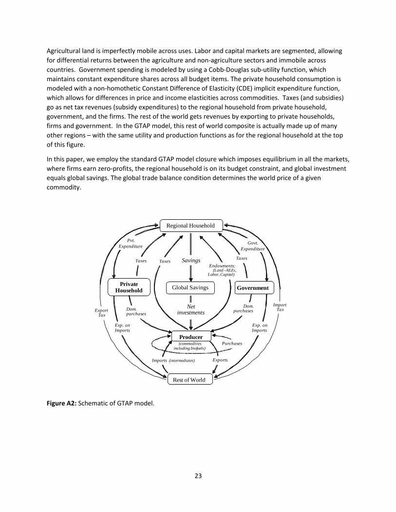
3. Additional Details on GTAP Model Structure

The Global Trade Analysis Project (GTAP) model is a multi-commodity, multi-regional computable

general equilibrium model documented in a book, published by Cambridge University Press (T. W.

Hertel, 1997) with detailed discussion on theory and derivation of the behavioral equations involved in

the model. The standard GTAP model employs the simple, but robust, assumptions of constant returns

to scale and perfect competition in all the markets with Walrasian adjustment to ensure a general

equilibrium. As represented in the figure below (Brockmeier, 2001), the regional household (e.g., the

EU) collects all the income in its region and spends it over three expenditure types – private household

(consumer), government, and savings, as governed by a Cobb-Douglas utility function. A representative

firm maximizes profits subject to a nested Constant Elasticity of Substitution (CES) production function

which combines primary factors and intermediates inputs to produce a final good. Firms pay

wages/rental rates to the regional household in return for the employment of land, labor, capital, and

natural resources. Firms sell their output to other firms (intermediate inputs), to private households,

government, and investment. Since this is a global model, firms also export the tradable commodities

and import the intermediate inputs from other regions. These goods are assumed to be differentiated

by region, following the Armington assumption, and so the model can track bilateral trade flows. See

Figure A2 for a schematic of the GTAP approach.

23

Agricultural land is imperfectly mobile across uses. Labor and capital markets are segmented, allowing

for differential returns between the agriculture and non-agriculture sectors and immobile across

countries. Government spending is modeled by using a Cobb-Douglas sub-utility function, which

maintains constant expenditure shares across all budget items. The private household consumption is

modeled with a non-homothetic Constant Difference of Elasticity (CDE) implicit expenditure function,

which allows for differences in price and income elasticities across commodities. Taxes (and subsidies)

go as net tax revenues (subsidy expenditures) to the regional household from private household,

government, and the firms. The rest of the world gets revenues by exporting to private households,

firms and government. In the GTAP model, this rest of world composite is actually made up of many

other regions – with the same utility and production functions as for the regional household at the top

of this figure.

In this paper, we employ the standard GTAP model closure which imposes equilibrium in all the markets,

where firms earn zero-profits, the regional household is on its budget constraint, and global investment

equals global savings. The global trade balance condition determines the world price of a given

commodity.

Rest of World

Savings

Net investments

Global Savings

Regional Household

Producer

Government Private

Household

Exports Imports (intermediates)

Govt.

Expenditure

Import Tax

Pvt.

Expenditure

Export Tax

Exp. on Imports

Exp. on Imports

Dom. purchases Dom.

purchases

Taxes Taxes

Taxes Endowments:

(Land -AEZs, Labor, Capital)

Purchases (commodities including biofuels)

Figure A2: Schematic of GTAP model.

24

4. Yield-Temperature Model Coefficients and Robustness Checks

Figure A3: Estimated yield response to CO2 fertilization (solid) line with 95% confidence intervals.

25

Model 1 Model 2 Model 3 Model 4

f(CO2) 18.55 ** 17.86 ** 18.01 ** 19.44 **

6.16 5.93 7.23 6.40

f(CO2)*C4 NA NA 1.24 NA

6.73

Rainfall 0.22 * 0.21 * 0.22 * 0.22 *

0.12 0.12 0.12 0.12

Adaptation 5.49 4.97 5.44 14.65 *

5.72 7.64 5.85 7.40

Adaptation*Tropical NA NA NA -9.11

9.09

Adaptation*Temp 0.13 0.27 0.12 2.19

2.04 2.09 2.05 2.43

Adaptation*Temp*Tropcial NA NA NA 3.91

4.38

Temp*Maize_Temperate -5.35 -11.61 -5.46 -8.10 *

4.46 7.95 4.71 4.95

Temp^2*Maize_Temperate 0.08 2.00 0.09 0.28

0.66 2.56 0.67 0.75

Temp^3*Maize_Temperate NA -0.16 NA NA

0.27

Temp*Maize_Tropical -6.70 -9.99 -6.80 -8.39

4.67 11.85 4.80 4.72

Temp^2*Maize_Tropical 0.10 -0.14 0.10 -0.10

0.90 6.15 0.90 1.01

Temp^3*Maize_Tropcial NA 0.18 NA NA

0.95

Temp*Wheat_Temperate -4.42 -14.89 -4.45 -7.46

5.70 10.20 5.81 5.81

Temp^2*Wheat_Temperate 0.28 5.23 0.30 0.55

1.11 4.59 1.18 1.08

Temp^3*Wheat_Temperate NA -0.63 NA NA

0.61

Temp*Wheat_Tropical -3.00 -7.52 -2.82 -5.51

4.41 7.47 4.37 4.40

Temp^2*Wheat_Tropical -1.71 ** -0.57 -1.73 ** -1.72 **

0.81 3.39 0.80 0.87

Temp^3*Wheat_Tropcial NA -0.08 NA NA

0.50

Temp*Rice -7.48 -19.72 ** -7.34 -9.90 **

4.74 9.23 4.77 4.51

Temp^2*Rice 0.83 6.61 0.82 0.84

0.79 4.18 0.79 0.77

Temp^3*Rice NA -0.72 NA NA

0.51

Temp*Soybeans -12.12 -26.69 -12.22 -14.35

3.78 28.20 12.52 12.94

26

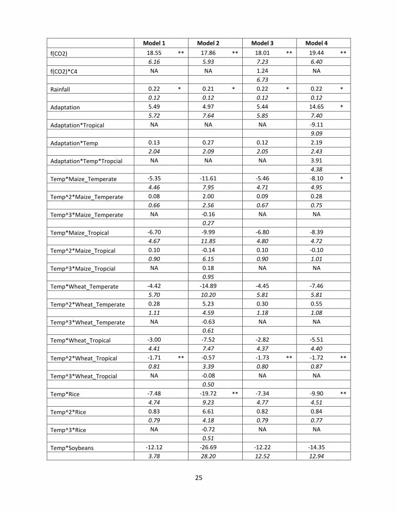
Table A1: Coefficients and standard errors (below in italics) of yield-response model estimated using Equation 1

(Model1) with three robustness checks. Model 2 includes cubic terms in the temperature response, Model 3 allows

for a different CO2 response for C4 crops, and Model 4 allows for different adaptation in temperate and tropical

regions. Interpretation of coefficients and standard errors for the non-linear temperature response are difficult to

interpret so these response functions and confidence intervals are given in Figure 1 (Model 1) and Figure A4

(Model 2). Standard errors are calculated from 750 block bootstraps, blocking at the study level.

Figure A4: Cubic temperature response functions from Model 1 (Table A1) and 95% confidence intervals based on

750 block bootstraps. Responses are shown for the preferred CO2 specification that includes CO2 fertilization for

the C3 crops (wheat, rice and soybeans) but not for maize. Results are quantitatively similar to the preferred

quadratic specification shown in Figure 1.

Temp^2*Soybeans 1.17 8.34 1.19 1.20

3.78 29.27 3.76 3.80

Temp^3*Soybeans NA -0.82 NA NA

7.26

27

5. Gridded Yield Changes

Figure A5: Example of gridded yield impacts products for 1-5 degrees of global temperature change derived using

the yield-temperature response functions (Figure 1) and the pattern scaling of local to global warming (Figure A1).

These show the effects on maize yields, excluding the CO2 fertilization effect. The boreal zone (shown in grey) is

excluded from the analysis.

28

6. Supplementary Results

Figure A6: Absolute welfare changes (equivalent variation) by FUND region for 3°C warming under the preferred

CO2 scenario. Changes are decomposed into the direct effect on yields, the allocative efficiency effect and the

terms-of-trade effect (see Section 3.2 for more discussion).