metals

Article

Fracture Toughness Calculation Method Amendmentof the Dissimilar Steel Welded Joint Based on3D XFEM

Yuwen Qian 1,2 and Jianping Zhao 1,2,*1 School of Mechanical and Power Engineering, Nanjing Tech University, Nanjing 211816, China;

reasonqiean@gmail.com2 Jiangsu Key Lab of Design and Manufacture of Extreme Pressure Equipment, Nanjing 211816, China* Correspondence: jpzhao71@njtech.edu.cn

Received: 21 March 2019; Accepted: 27 April 2019; Published: 30 April 2019�����������������

Abstract: The dissimilar steel welded joint is divided into three pieces, parent material–weldmetal–parent material, by the integrity identification of BS7910-2013. In reality, the undermatchedwelded joint geometry is different: parent material–heat affected zone (HAZ)–fusion line–weld metal.A combination of the CF62 (parent material) and E316L (welding rod) was the example undermatchedwelded joint, whose geometry was divided into four pieces to investigate the fracture toughness of thejoint by experiments and the extended finite element method (XFEM) calculation. The experimentalresults were used to change the fracture toughness of the undermatched welded joint, and the XFEMresults were used to amend the fracture toughness calculation method with a new definition of thecrack length. The research results show that the amendment of the undermatched welded jointgeometry expresses more accuracy of the fracture toughness of the joint. The XFEM models wereverified as valid by the experiment. The amendment of the fracture toughness calculation methodexpresses a better fit by the new definition of the crack length, in accordance with the crack routesimulated by the XFEM. The results after the amendment coincide with the reality in engineering.

Keywords: undermatched; integrity identification; XFEM; fracture toughness calculation method

1. Introduction

1.1. The Undermatched Welded Joint

High-strength low-alloy (HSLA) steel is commonly used for petrochemical equipment.The development of special electrodes for the new HSLA is expensive and time-consuming. Ready-madelower strength electrodes for HSLA are a good choice to fabricate the undermatched welded joint.The undermatched welded joint has a low crack tendency and is economical within a wide range ofmatching ratios [1].

1.2. The Integrity Identification of the Undermatched Welded Joint

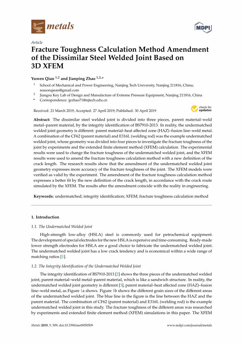
The integrity identification of BS7910-2013 [2] shows the three pieces of the undermatched weldedjoint, parent material–weld metal–parent material, which is like a sandwich structure. In reality, theundermatched welded joint geometry is different [3], parent material–heat affected zone (HAZ)–fusionline–weld metal, as Figure 1a shows. Figure 1b shows the different grain sizes of the different areasof the undermatched welded joint. The blue line in the figure is the line between the HAZ and theparent material. The combination of CF62 (parent material) and E316L (welding rod) is the exampleundermatched welded joint in this study. The fracture toughness of the different areas was researchedby experiments and extended finite element method (XFEM) simulations in this paper. The XFEM

Metals 2019, 9, 509; doi:10.3390/met9050509 www.mdpi.com/journal/metals

Metals 2019, 9, 509 2 of 16

models of the different areas of the undermatched welded joint were built and verified as valid bythe experiments.

Figure 1. Different areas of the investigated welded joint. (a) Different local areas; (b) Grain.

1.3. The Research Status of XFEM

The extended finite element method (XFEM) was put forward by Belytschko [4], an Americanprofessor, and was used to research the crack growth route. Compared to the traditional finite element,the XFEM simulated the crack initiation and growth without the need to refresh the meshing, reducingthe workload. Sukumar et al. [5] promoted the 2D XFEM crack model to a 3D XFEM crack model.Legay [6] and Ventura et al. [7] researched the blending element (shown in Figure 2) to improve theconvergence and precision of the simulation. Menouillard [8] improved integral stability. Zhuang andCheng [9] realized the fusion line crack extension between the dissimilar steels by the XFEM.

Figure 2. Planar crack, cut element, and blending element.

Research of the XFEM began late in China. Xiujun Fang of Tsinghua University researchedthe cohesive crack model based on the XFEM in 2007 [10]. Hai Xie of Shanghai Jiaotong Universitydeveloped the XFEM with the ABAQUS User Subroutine in 2009 [11]. Yehai Li of Nanjing Universityof Aeronautics and Astronautics researched the interfacial crack growth of the dissimilar material in2012 [12]. Shaoyun Zhang of Zhejiang University researched the helical crack growth by the XFEM in2013 [13]. Zhifeng Yang of Nanjing Tech University developed the 2D elastic-plastic crack XFEM modeland verified its validity by the J integral in 2014 [14]. Yixiu Shu of the Northwestern PolytechnicalUniversity analyzed the multiple crack interaction problems by the XFEM in 2015 [15]. Yang Zhang ofHarbin Engineering University applied a 3D crack to the pressure vessel by the XFEM in 2015 [16].Zhen Wang and Tiantang Yu researched the adaptive multiscale XFEM model for 3D crack problems in2016 [17].

Metals 2019, 9, 509 3 of 16

1.4. The Welding of the Undermatched Joint

The size of the weld plate is 600 × 400 × 40 mm (length, width, and thickness, respectively) with anX-shaped groove, shown in Figure 3. The welding rod (E316L) is the special electrode for 316L stainlesssteel. The welding parameters are listed in Table 1, in accordance with the criteria of ASME-VIII [18].Tables 2 and 3 list the chemical composition tested results of CF62 and E316L. Tables 4 and 5 list themechanical properties of the CF62 steel and the E316L steel, respectively.

Figure 3. The investigated welded joint.

Table 1. Welding parameters of the undermatched welded joint adapted from [18], with permissionfrom American Society of Mechanical Engineers, 2019.

LayerName

LayerNumbers

Voltage(V)

Current(A)

Welding Speed(cm/min)

Backing Welding 1 20 75 9Filler Welding 2–11 22 79.5 10.5Cover Welding 12–13 24 105 15

Table 2. Chemical composition of CF62 (wt.%).

C Mn Si S P Cr Mo V B

0.121 1.260 0.188 0.002 0.011 0.224 0.213 0.035 0.001

Table 3. Chemical composition of E316L(wt.%).

C Cr Ni Mo Si Mn P S Co

0.039 18.96 10.73 2.33 0.62 1.06 0.02 0.0064 0.025

Table 4. Mechanical properties of CF62 reproduced from [19], with permission from Taiyuan Universityof Science and Technology, 2019.

Temperature(◦C)

Heat ConductivityCoefficient

(W·m−1·◦C−1)

Density(kg·m−3)

Specific Heat(J·kg−1·◦C−1)

ElasticModulus

(GPa)

Poisson’sRatio

YieldStrength

(MPa)

ThermalExpansivity

(10−6·mm/mm/K)

25 51.25 7860 450 209 0.29 575 0.01100 47.95 7840 480 204 0.29 550 0.09200 44.13 7810 520 200 0.30 520 0.23400 38.29 7740 620 175 0.31 438 0.51600 34.65 7670 810 135 0.31 280 0.82800 29.59 7630 990 78 0.33 80 0.971000 29.35 7570 620 15 0.35 30 1.241200 31.88 7470 660 3 0.36 10 1.701400 34.4 7380 690 1 0.38 5 2.161600 34.79 6940 830 1 0.50 5 4.391640 335 6940 830 1 0.50 5 4.39

Metals 2019, 9, 509 4 of 16

Table 5. Mechanical properties of E316L reproduced from [20], with permission from weldingtechnology, 2019.

Temperature(◦C)

Heat ConductivityCoefficient

(W·m−1·◦C−1)

Density(kg·m−3)

Specific Heat(J·kg−1·◦C−1)

ElasticModulus

(GPa)

Poisson’sRatio

YieldStrength

(MPa)

ThermalExpansivity

(10−6·mm/mm/K)

20 13.31 7966 470 195.1 0.267 325 15.24200 16.33 7893 508 185.7 0.29 226 16.43400 19.47 7814 550 172.6 0.322 180 17.44600 22.38 7724 592 155 0.296 165 18.21800 25.07 7630 634 131.4 0.262 153 18.83900 26.33 7583 655 116.8 0.24 100 19.111000 27.53 7535 676 100.1 0.229 53 19.381100 28.67 7486 698 81.1 0.223 23 19.661200 29.76 7436 719 59.5 0.223 15 19.951420 31.95 7320 765 2 0.223 3.3 20.71460 320 7320 765 2 0.223 3.3 20.7

1.5. The Fracture Toughness Calculation Method

ASTM 1820-18 [21] is the newest standard test method for the measurement of fracture toughness.Fracture toughness is calculated by the relationship between the J integral and the crack length, ai [21]:

J =K2

(1− ν2

)E

+ Jpl (1)

Jpl =ηplApl

BNbo(2)

where:

Apl is the area under force versus displacement, as shown in Figure 4;

ηpl is either 1.9 if the load-line displacement is used for Apl or 3.667 − 2.199(a0/w) + 0.437(a0/w)2 if therecorded crack mouth opening displacement is used for Apl;

BN is the net specimen thickness;bo is W − a0.

Figure 4. Definition of the area for the J calculation using the basic method.

The crack length, ai, is calculated by the displaced force point with Equation (3):

aiW

= 1.000196− 4.06319µ+ 11.242µ2− 106.043µ3 + 464.335µ4

− 650.677µ5 (3)

Metals 2019, 9, 509 5 of 16

where:µ =

1(BeE Cc(i)

)1/2+ 1

(4)

Be = B− (B− BN)2/B (5)

Cc(i) =Ci(

H∗Ri

sinθi − cosθi)(

DRi

sinθi − cosθi) (6)

where:

Ci is the measured specimen elastic compliance (∆vm/∆Pm) (at the load-line);H∗ is the initial half-span of the load points (center of the pin holes);D is one-half of the initial distance between the displacement measurement points;Ri is the radius of the rotation of the crack center line, (W+a)/2, where a is the updated crack size.

Figure 5a shows the relationship between the crack rotation angle, θi, and the respective cracklength, ai [21]. The crack rotation angle, θi, is calculated by Equation (7). Figure 5a shows that thecrack length, ai, was equal to the length parallel to the center line of the compact tension (CT) samples.The crack deflection has not been considered in the crack length calculation in the criteria.

θi = sin−1{(

D +Vm{i}

2

)/[D2 + R2

i

]1/2}− tan−1(

DRi

) (7)

where Vm(i) is the total measured load-line displacement at the beginning of the i-thunloading/reloading cycle.

Figure 5. Crack rotation angle, θ, of the compact tension (CT) specimens. (a) Initial crack; (b) Crackafter deflection.

Figure 5b shows the crack route after the crack deflection. It shows the crack length after the

deflection, a =√

ax2 + ay2. The crack length in the criteria of ASTM 1820-18 is ai = ay, which meansthat ai < a. Therefore, the crack length, ai, calculated by the criteria of ASTM 1820-18, was smallerthan the true crack length after the deflection, a. The fracture toughness calculation method was thenamended by the crack length after the deflection was simulated by the XFEM.

The division of the geometry (parent material–HAZ–fusion line–weld metal) of the undermatchedwelded joint and the experimental results changed the fracture toughness of the dissimilar steel weldedjoint. The crack length amendment after the deflection defined a new fracture toughness calculationmethod of the dissimilar welded joint.

Metals 2019, 9, 509 6 of 16

1.6. J Integral and the Fracture Toughness Value,Kmat

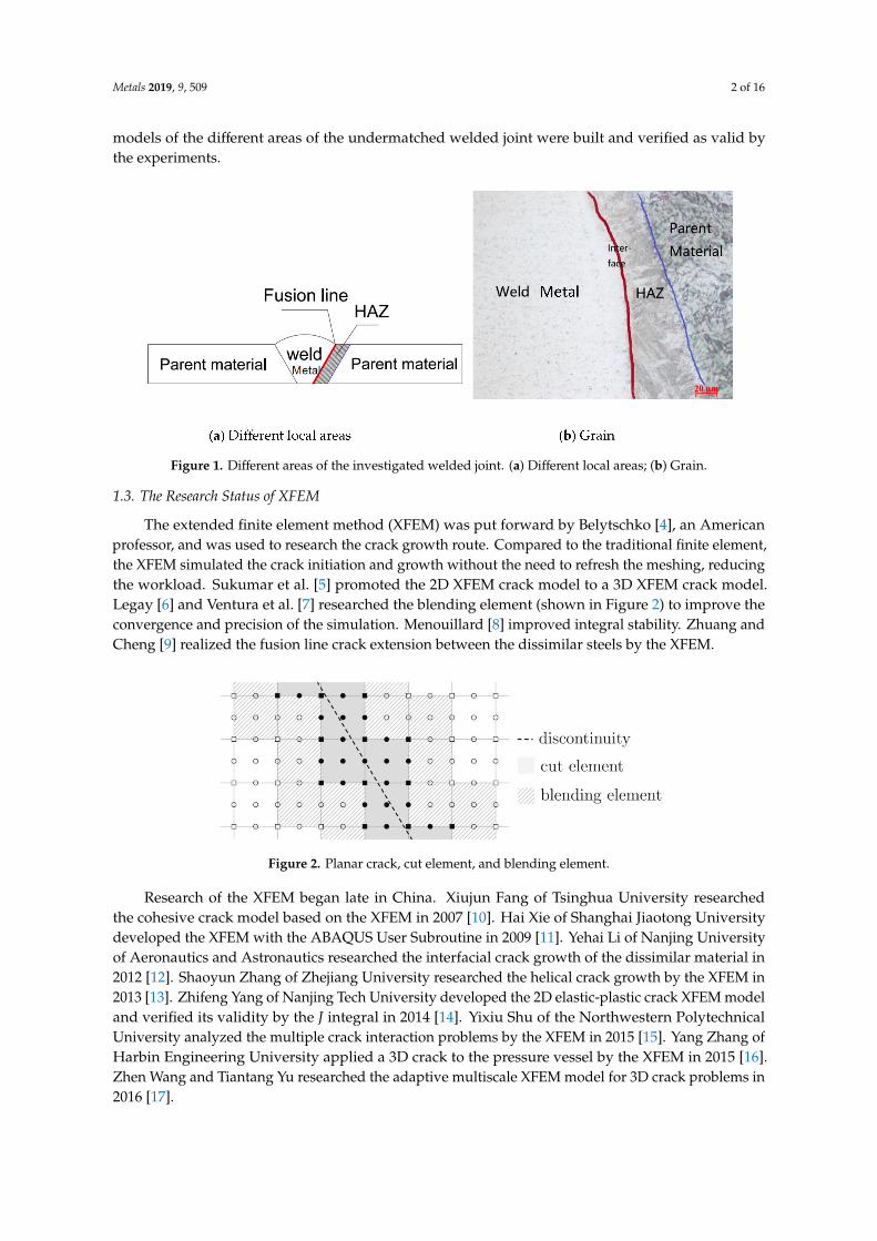
The J integral was put forward by Rice [22]. Figure 6a shows the integral loop/area around thecrack tip. Equation (8) is calculated with the equivalent integral region to deal with the stress and thestrain of Figure 6b [22]. Figure 6c shows the integral area, which contains a heterogeneous materialinterface. In [23], it was verified that the interface integral area Ith

A+ = IthA− = Iinter f ace = 0 when the

crack tip is under a constant temperature with a pure mechanical load. Equation (8) is applicable tocalculate the J integral for the investigated welded joint in this paper.

J =∫

A

(σi j∂u j

∂x1−ωδ1i

)∂q∂xi

dA (8)

where ui is the component of the displacement vector; dA is the tiny increment area on the integralpath, Γ; ω is the strain energy density factor; and q(x,y) is a mathematical function, which is q = 0 in theouter boundary and q = 1 in the other places of the regional; and ω, Ti are listed in Equation (9).

ω =

εi j∫0σi jdεi j

Ti = σi jn j

(9)

where σi j is the stress tensor and εi j is the strain tensor.

Figure 6. Counterclockwise integral loop around the crack tip. (a) Integral loop; (b) Integral area;(c) Interface integral area.

Metals 2019, 9, 509 7 of 16

BS7910-2013 [2] gives Equation (10), which shows the relationship between the Jmat value and thefracture toughness value, Kmat, during the elastic stage:

Jmat =K2

mat

(1− ν2

)E

(10)

where E is the elastic modulus and ν is the Poisson’s ratio.

2. Experiments

2.1. The Fracture Toughness Experiments

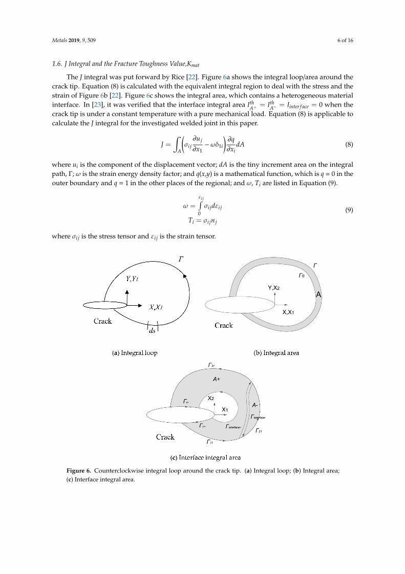
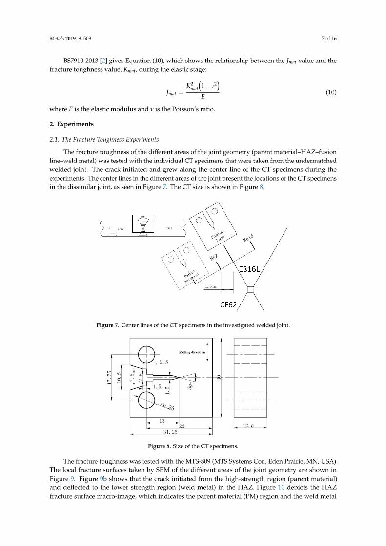
The fracture toughness of the different areas of the joint geometry (parent material–HAZ–fusionline–weld metal) was tested with the individual CT specimens that were taken from the undermatchedwelded joint. The crack initiated and grew along the center line of the CT specimens during theexperiments. The center lines in the different areas of the joint present the locations of the CT specimensin the dissimilar joint, as seen in Figure 7. The CT size is shown in Figure 8.

Figure 7. Center lines of the CT specimens in the investigated welded joint.

Figure 8. Size of the CT specimens.

The fracture toughness was tested with the MTS-809 (MTS Systems Cor., Eden Prairie, MN, USA).The local fracture surfaces taken by SEM of the different areas of the joint geometry are shown inFigure 9. Figure 9b shows that the crack initiated from the high-strength region (parent material)and deflected to the lower strength region (weld metal) in the HAZ. Figure 10 depicts the HAZfracture surface macro-image, which indicates the parent material (PM) region and the weld metal

Metals 2019, 9, 509 8 of 16

region. It means that the crack deflection existed in the dissimilar material during the experiment.The experimental process was in accordance with the criteria of ASTM 1820-18 [21], and the results ofthe J integral and the crack length, ∆a, were managed under the regulations.

Figure 9. Fracture surfaces after the fracture toughness experiment. (a) Parent material (PM); (b) HAZ;(c) Fusion line; (d) Weld metal.

Figure 10. HAZ fracture surface macro-image.

2.2. The Tensile Experiments

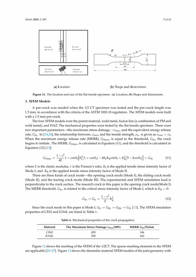
The maximum stress damage of the parent material and the weld metal was needed to build theXFEM models. It was tested with a flat tensile specimen, which was 0.8 mm in thickness. Figure 11ashows the location of the tensile specimen, which was taken from the parent material to the weld metaland is parallel to the fusion line. Figure 11b shows the shape and dimensions of the flat tensile specimen.

Metals 2019, 9, 509 9 of 16

Figure 11. The location and size of the flat tensile specimen. (a) Location; (b) Shape and dimensions.

3. XFEM Models

A pre-crack was needed when the 1/2 CT specimen was tested and the pre-crack length was1.5 mm, in accordance with the criteria of the ASTM 1820-18 regulation. The XFEM models were builtwith a 1.5 mm pre-crack.

The four XFEM models were the parent material, weld metal, fusion line (a combination of PM andweld metal), and HAZ. The mechanical properties were tested by the flat tensile specimen. There weretwo important parameters—the maximum stress damage, −σmax, and the equivalent energy releaserate, Gθc. In [14,24], the relationship between, σmax, and the tensile strength, σb, is given as σmax = σb.When the maximum energy release rate (MERR), Gθmax, is equal to the threshold, Gθc, the crackbegins to initiate. The MERR, Gθmax, is calculated in Equation (11), and the threshold is calculated inEquation (12) [13]:

Gθmax =1− ν2

4E1 + cosθ0

[K2

I [1 + cosθ0] − 4KIKIIsinθ0 + K2II[5− 3cosθ0]

]= Gθc (11)

where E is the elastic modulus, ν is the Poisson’s ratio, KI is the applied tensile stress intensity factor ofMode I, and KII is the applied tensile stress intensity factor of Mode II.

There are three kinds of crack mode—the opening crack mode (Mode I), the sliding crack mode(Mode II), and the tearing crack mode (Mode III). The experimental and XFEM simulation load isperpendicular to the crack surface. The research crack in this paper is the opening crack mode(Mode I).The MERR threshold, Gθc, is related to the critical stress intensity factor of Mode I, which is KII = 0:

Gθc = GIc =1− ν2

EK2

Ic (12)

Since the crack mode in this paper is Mode I, GIc = GIIc = GIIIc = Gθc [13]. The XFEM simulationproperties of CF62 and E316L are listed in Table 6.

Table 6. Mechanical properties of the crack propagation.

Material The Maximum Stress Damage σmax/MPa MERR Gθc/N/mm

CF62 650 146E316L 550 160

Figure 12 shows the meshing of the XFEM of the 1/2CT. The sparse meshing elements in the XFEMare applicable [25–27]. Figure 13 shows the dissimilar material XFEM models of the joint geometry with

Metals 2019, 9, 509 10 of 16

the material printed on their parts. The parent material and weld metal XFEM models are not shownsince they are the uniform material model, i.e., they are the material printed on the whole model.

Figure 12. The meshing model of the extended finite element method(XFEM).

Figure 13. The dissimilar material XFEM models. (a) Fusion line; (b) HAZ.

4. The Fracture Toughness of the Undermatched Welded Joint

4.1. Fracture Toughness of the Undermatched Welded Joint

The test results of the J integral and crack length, ∆a, are fitted by Equation (13) in the criteria ofASTM 1820-18 [21]:

J = α+ β(∆a)r (13)

The experimental data and the resistance equations of the different areas of the joint geometry arelisted in Tables 7 and 8, respectively. The resistance curves are shown in Figure 14.

Table 7. Experimental data.

Data Parent Material HAZ Fusion Line Weld MetalPoints ∆a/mm J/KJ/m2 ∆a/mm J/KJ/m2 ∆a/mm J/KJ/m2 ∆a/mm J/KJ/m2

1 0 0 0 0 0 0 0 02 0.133 118.03 0.478 276.52 0.439 181.30 0.265 116.203 0.318 191.35 0.623 315.80 0.624 230.76 0.509 223.114 0.496 309.24 1.277 438.68 0.869 245.48 0.611 278.275 1.073 423.93 1.821 562.78 1.101 296.98 0.872 331.576 1.234 514.53 3.396 328.69 1.478 332.97 1.144 359.877 1.433 606.27 3.851 326.04 1.939 354.85 1.535 373.71

Metals 2019, 9, 509 11 of 16

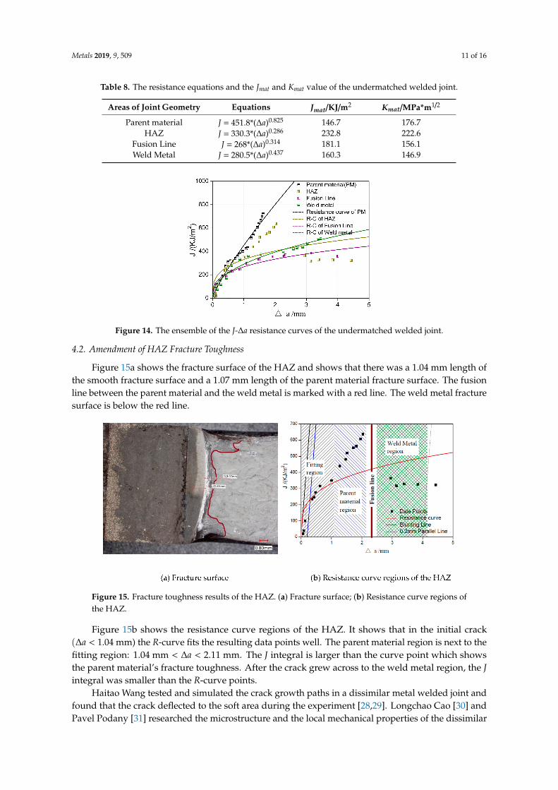
Table 8. The resistance equations and the Jmat and Kmat value of the undermatched welded joint.

Areas of Joint Geometry Equations Jmat/KJ/m2 Kmat/MPa*m1/2

Parent material J = 451.8*(∆a)0.825 146.7 176.7HAZ J = 330.3*(∆a)0.286 232.8 222.6

Fusion Line J = 268*(∆a)0.314 181.1 156.1Weld Metal J = 280.5*(∆a)0.437 160.3 146.9

Figure 14. The ensemble of the J-∆a resistance curves of the undermatched welded joint.

4.2. Amendment of HAZ Fracture Toughness

Figure 15a shows the fracture surface of the HAZ and shows that there was a 1.04 mm length ofthe smooth fracture surface and a 1.07 mm length of the parent material fracture surface. The fusionline between the parent material and the weld metal is marked with a red line. The weld metal fracturesurface is below the red line.

Figure 15. Fracture toughness results of the HAZ. (a) Fracture surface; (b) Resistance curve regions ofthe HAZ.

Figure 15b shows the resistance curve regions of the HAZ. It shows that in the initial crack(∆a < 1.04 mm) the R-curve fits the resulting data points well. The parent material region is next to thefitting region: 1.04 mm < ∆a < 2.11 mm. The J integral is larger than the curve point which showsthe parent material’s fracture toughness. After the crack grew across to the weld metal region, the Jintegral was smaller than the R-curve points.

Haitao Wang tested and simulated the crack growth paths in a dissimilar metal welded joint andfound that the crack deflected to the soft area during the experiment [28,29]. Longchao Cao [30] andPavel Podany [31] researched the microstructure and the local mechanical properties of the dissimilar

Metals 2019, 9, 509 12 of 16

butt joints. Jianbo Li [32] studied the fracture toughness near the fusion line (HAZ and fusion line) ofthe dissimilar material and, in addition, found the crack deflection. The HAZ experimental resultsdemonstrated the crack deflection when the CT specimens were tested. The resistance curve of theHAZ (Figure 15b) shows that the fracture toughness of the undermatched welded joint needs to beamended. The crack deflection shows that the crack length test method needs to be amended as well.

As there was a misfit of the data points in the two regions and the lower strength region wasthe weld metal region, which was below the high-strength region, the HAZ was considered to be thehigh-strength region. The crack initiated in the HAZ high-strength region and then deflected to theweld metal region. During the crack growth process, the crack crossed the fusion line between thehigh-strength region and the weld metal region. Figure 9b shows the local fracture surface figuretaken by SEM, which shows the location of the high-strength region and the weld metal region (lowerstrength region).

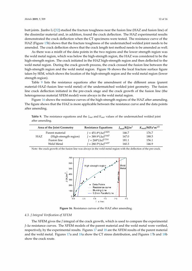
Table 9 lists the resistance equations after the amendment of the different areas (parentmaterial–HAZ–fusion line–weld metal) of the undermatched welded joint geometry. The fusionline crack deflection initiated in the pre-crack stage and the crack growth of the fusion line (theheterogeneous material XFEM model) were always in the weld metal region.

Figure 16 shows the resistance curves of the high-strength regions of the HAZ after amending.The figure shows that the HAZ is more applicable between the resistance curve and the data pointsafter amending.

Table 9. The resistance equations and the Jmat and Kmat values of the undermatched welded jointafter amending.

Area of the Joint Geometry Resistance Equations Jmat/KJ/m2 Kmat/MPa*m1/2

Parent material J = 451.8*(∆a)0.825 146.7 176.7HAZ (High-strength region) J = 389.9*(∆a)0.647 167.0 188.5

Fusion line J = 268*(∆a)0.314 181.1 156.1Weld Metal J = 280.5*(∆a)0.437 160.3 146.9

Note: the crack growth of the fusion line was always in the weld metal region with the deflection of the pre-crack.

Figure 16. Resistance curves of the HAZ after amending.

4.3. J Integral Verification of XFEM

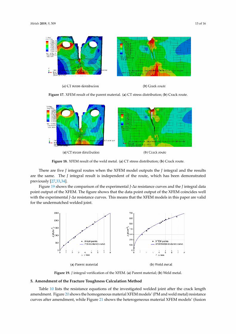
The XFEM gives the J integral of the crack growth, which is used to compare the experimentalJ-∆a resistance curves. The XFEM models of the parent material and the weld metal were verified,respectively, by the experimental results. Figures 17 and 18 are the XFEM results of the parent materialand the weld metal. Figures 17a and 18a show the CT stress distribution, and Figures 17b and 18bshow the crack route.

Metals 2019, 9, 509 13 of 16

Figure 17. XFEM result of the parent material. (a) CT stress distribution; (b) Crack route.

Figure 18. XFEM result of the weld metal. (a) CT stress distribution; (b) Crack route.

There are five J integral routes when the XFEM model outputs the J integral and the resultsare the same. The J integral result is independent of the route, which has been demonstratedpreviously [27,33,34].

Figure 19 shows the comparison of the experimental J-∆a resistance curves and the J integral datapoint output of the XFEM. The figure shows that the data point output of the XFEM coincides wellwith the experimental J-∆a resistance curves. This means that the XFEM models in this paper are validfor the undermatched welded joint.

Figure 19. J integral verification of the XFEM. (a) Parent material; (b) Weld metal.

5. Amendment of the Fracture Toughness Calculation Method

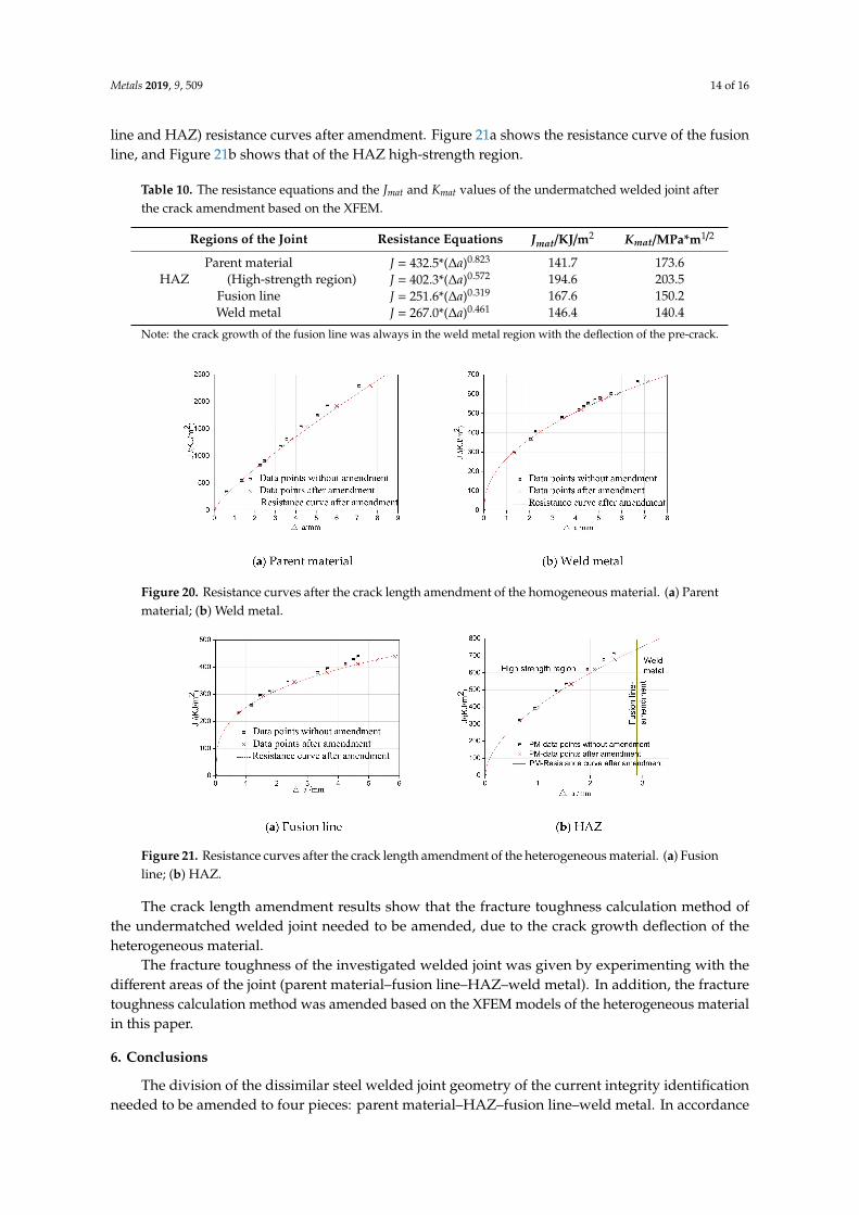
Table 10 lists the resistance equations of the investigated welded joint after the crack lengthamendment. Figure 20 shows the homogeneous material XFEM models’ (PM and weld metal) resistancecurves after amendment, while Figure 21 shows the heterogeneous material XFEM models’ (fusion

Metals 2019, 9, 509 14 of 16

line and HAZ) resistance curves after amendment. Figure 21a shows the resistance curve of the fusionline, and Figure 21b shows that of the HAZ high-strength region.

Table 10. The resistance equations and the Jmat and Kmat values of the undermatched welded joint afterthe crack amendment based on the XFEM.

Regions of the Joint Resistance Equations Jmat/KJ/m2 Kmat/MPa*m1/2

Parent material J = 432.5*(∆a)0.823 141.7 173.6HAZ (High-strength region) J = 402.3*(∆a)0.572 194.6 203.5

Fusion line J = 251.6*(∆a)0.319 167.6 150.2Weld metal J = 267.0*(∆a)0.461 146.4 140.4

Note: the crack growth of the fusion line was always in the weld metal region with the deflection of the pre-crack.

Figure 20. Resistance curves after the crack length amendment of the homogeneous material. (a) Parentmaterial; (b) Weld metal.

Figure 21. Resistance curves after the crack length amendment of the heterogeneous material. (a) Fusionline; (b) HAZ.

The crack length amendment results show that the fracture toughness calculation method ofthe undermatched welded joint needed to be amended, due to the crack growth deflection of theheterogeneous material.

The fracture toughness of the investigated welded joint was given by experimenting with thedifferent areas of the joint (parent material–fusion line–HAZ–weld metal). In addition, the fracturetoughness calculation method was amended based on the XFEM models of the heterogeneous materialin this paper.

6. Conclusions

The division of the dissimilar steel welded joint geometry of the current integrity identificationneeded to be amended to four pieces: parent material–HAZ–fusion line–weld metal. In accordance

Metals 2019, 9, 509 15 of 16

with this new division of the undermatched welded joint, XFEM models of the undermatched weldedjoint were built to calculate their fracture toughness. The conclusions are as follows:

(1) The different areas (parent material–HAZ–fusion line–weld metal) of the undermatched weldedjoint geometry were tested to obtain the fracture toughness of the investigated welded joint.During the experiments, the fracture toughness of the joint changed in accordance with thecrack deflection.

(2) In this study, XFEM models of the homogeneous material and the heterogeneous material, i.e., thedifferent areas of the undermatched welded joint geometry, were built to calculate the crack route.

(3) The experimental results of the J-∆a resistance curve were compared to the XFEM calculationresults to verify the validity of the XFEM to the undermatched welded joint.

(4) The crack length amendment was in accordance with the XFEM simulation result—the crackroute. The fracture toughness calculation method was amended by the crack length amendmentafter the deflection of the heterogeneous material by the XFEM.

Author Contributions: Y.Q. is mainly on the Methodology, Software, Validation, Formal Analysis, Investigation,Data Curation, Writing-Original Draft Preparation, Writing-Review & Editing. J.Z. is mainly on Writing-Review &Editing, Visualization, Supervision, Funding Acquisition.

Funding: This research was funded by the National Key Research and Development Program of China[2016YFC0801905].

Conflicts of Interest: The authors declare no conflict of interest.

References

1. Wen, X.; Wang, P.; Dong, Z.B.; Liu, Y.; Fang, H.Y. Nominal stress-based equal-fatigue bearing-capacity designof under-matched HSLA steel butt-welded joints. Metals 2018, 8, 880. [CrossRef]

2. BS7910:2013+A1:2015, Guide to Methods for Assessing the Acceptability of Flaws in Metallic Structures; BSIStandards Limited: London, UK, 2015.

3. Baris Basyigit, A.; Murat, M.G. The Effects of TIG Welding Rod Compositions on Microstructural andMechanical Properties of Dissimilar AISI 304L and 420 Stainless Steel Welds. Metals 2018, 8, 972. [CrossRef]

4. Belytschko, T.; Black, T. Elastic crack growth in finite elements with minimal remeshing. Int. J. Numer.Methods Eng. 1999, 45, 601–620. [CrossRef]

5. Sukumar, N.; Moes, N.; Moran, B.; Belytschko, T. Extended finite element method for three-dimensionalcrack modeling. Int. J. Numer. Methods Eng. 2000, 48, 1549–1570. [CrossRef]

6. Legay, A.; Wang, H.W.; Belytschko, T. Strong and weak arbitrary discontinuities in spectral finite elements.Int. J. Numer. Methods Eng. 2005, 64, 991–1008. [CrossRef]

7. Ventura, G.; Moran, B.; Belytschko, T. Dislocations by partition of unity. Int. J. Numer. Methods Eng. 2005, 62,1463–1487. [CrossRef]

8. Menouillard, T.; Rethore, J.; Combescure, A.; Bung, H. Efficient explicit time stepping for the extended finiteelement method (XFEM). Int. J. Numer. Methods Eng. 2006, 68, 911–939. [CrossRef]

9. Zhuang, Z.; Cheng, B.B. Equilibrium state of mode-I sub-interfacial crack growth in bi-materials. Int. J. Fract.2011, 170, 27–36. [CrossRef]

10. Fang, X.J.; Jin, F.; Wang, J.T. Cohesive crack model based on extended finite element method. J. TsinghuaUniv. Sci. Tech. 2007, 47, 344–347. (In Chinese)

11. Xie, H.; Feng, M.L. Implementation of Extended Finite Element Method with ABAQUS User Subroutine. J.Shanghai Jiaotong Univ. 2009, 43, 1644–1648. (In Chinese)

12. Li, Y. Research on Interfacial Crack Propagation Using ABAQUS: Application to Artificial Ice Shape. Ph.D.Thesis, Nanjing University of Aeronautics and Astronautics, Nanjing, China, 2012. (In Chinese).

13. Zhang, S. Study on Helical Crack Propagation by Extended Finite Element Method. Ph.D. Thesis, ZhejiangUniversity, Hangzhou, China, 2013. (In Chinese).

14. Yang, Z.; Zhou, C.; Dai, Q. Elastic-plastic crack propagation based on extended finite element method. J.Nanjing Tech Univ. (Nat. Sci. Ed.) 2014, 36, 50–57. (In Chinese)

Metals 2019, 9, 509 16 of 16

15. Shu, Y.X.; Li, Y.Z.; Jiang, W.; Jia, Y.X. Analyzing Multiple Crack Propagation Using Extended Finite ElementMethod(X-FEM). J. Northwest. Polytech. Univ. 2015, 33, 197–203. (In Chinese)

16. Zhang, Y. Application Research of the Extended Finite Element Method on the Cracks in Pressure Vessel.Ph.D. Thesis, Harbin Engineering University, Harbin, China, 2015. (In Chinese).

17. Wang, Z.; Yu, T.T. Adaptive multiscale extended finite element method for modeling three-dimensional crackproblems. Eng. Mech. 2016, 33, 32–38. (In Chinese)

18. ASME. ASME Boiler & Pressure Vessel Code, Section VIII, Division 1; American Society of Mechanical Engineers:New York, NY, USA, 2010.

19. Gan, H. Effect of Cold Treatment Temperature on Microstructure and Mechanical Properties of Forged LowAlloy High Strength Steel. Ph.D. Thesis, Taiyuan University of Science and Technology, Taiyuan, China, 2012.(In Chinese).

20. Zhu, P.; Chen, Y.; Wang, G.G. Effect of high temperature tempering heat treatment on deposited metalproperties of nuclear grade E316L stainless steel welding rod. Weld. Technol. 2016, 45, 51–54. (In Chinese)

21. ASTM E1820-18. Standard test methods for measurement of fracture toughness. In Annual Book of ASTMStandards; American Society for Testing and Materials: Philadelphia, PA, USA, 2018; Volume 3.01.

22. Rice, J.R. A Path independent integral and the approximate analysis of strain concentration by notched andcracks. J. Appl. Mech. 1968, 35, 379–386. [CrossRef]

23. Guo, F. Investigation on the Thermal Fracture Mechanics of Nonhomogeneous Materials with Interfaces.Ph.D. Thesis, Harbin Institute of Technology, Harbin, China, 2014. (In Chinese).

24. Yang, Z. Limit Load Research of Crack Structure Based on Extended Finite Element Method. Ph.D. Thesis,Nanjing Tech University, Nanjing, China, 2014. (In Chinese).

25. Banasal, M.; Singh, I.V.; Mishra, B.K.; Bordas, S.P.A. A parallel and efficient multi-split XFEM for 3-D analysisof heterogeneous materials. Comput. Methods Appl. Mech. Eng. 2019, 347, 365–401. [CrossRef]

26. Sim, J.M.; Chang, Y.-S. Crack growth evaluation by XFEM for nuclear pipes considering thermal agingembrittlement effect. Fatigue Fract. Eng. Mater. Struct. 2019, 42, 775–791. [CrossRef]

27. Dai, Q.; Zhou, C.Y.; Peng, J.; He, X.H. Finite Element Analysis and EPRI Solution for J-integral of CommerciallyPure Titanium. Rare Metal. Mater. Eng. 2014, 43, 257–263.

28. Wang, H.T.; Wang, G.Z.; Xuan, F.Z.; Tu, S.T. An experimental investigation of local fracture resistance andcrack growth paths in a dissimilar metal welded joint. Mater. Des. 2013, 44, 179–189. [CrossRef]

29. Wang, H.T.; Wang, G.Z.; Xuan, F.Z.; Tu, S.T. Numerical investigation of ductile crack growth behavior in adissimilar metal welded joint. Nucl. Eng. des. 2011, 241, 3234–3243. [CrossRef]

30. Cao, L.C.; Shao, X.Y.; Jiang, P.; Zhou, Q.; Rong, Y.N.; Geng, S.N.; Mi, G.Y. Effects of Welding Speed onMicrostructure and Mechanical Property of Fiber Laser Welded Dissimilar Butt Joints between AISI316L andEH36. Metals 2013, 7, 270. [CrossRef]

31. Podany, P.; Reardon, C.; Koukolikova, M.; Prochazka, R.; Franc, A. Microstructure, Mechanical Propertiesand Welding of Low Carbon, Medium Manganese TWIP/TRIP Steel. Metals 2018, 8, 263. [CrossRef]

32. Li, J.B.; Liu, B.; Wang, Y. A Study on the Zener-Holloman Parameter and Fracture Toughness of anNb-Particles-Toughened TiAl-Nb Alloy. Metals 2018, 8, 387. [CrossRef]

33. Dai, Q.; Zhou, C.; Peng, J. Non-probabilistic Failure Assessment Methodology about Titanium Pipes withCracks. In Proceedings of the ASME 2011 Pressure Vessels and Piping Conference, Baltimore, MD, USA,17–21 July 2011.

34. Dai, Q.; Zhou, C.Y.; Peng, J. Non-probabilistic defect assessment for structures with cracks based on intervalmodel. Nucl. Eng. Des. 2013, 262, 235–245. [CrossRef]

© 2019 by the authors. Licensee MDPI, Basel, Switzerland. This article is an open accessarticle distributed under the terms and conditions of the Creative Commons Attribution(CC BY) license (http://creativecommons.org/licenses/by/4.0/).