Fracture patterns in a fold – a case

study from Bude, UK

Ingvild Næss

Master thesis in Structural Geology

Department of Earth Science

University of Bergen

March 2021

I

Abstract

Fracture patterns in a well-exposed folded Carboniferous sandstone and shale sequence at

Bude, SW England, have been analysed, and the use of such surface analogues for modelling

fracture systems is discussed. Each fracture is identified as a vein or a joint, or as a “fracture”,

if it is unclear whether it is a vein or a joint. These fracture types are a basis for defining sets,

along with orientations and relative ages. Seven fractures sets have been identified

individually at each limb and at the crest of the Whaleback fold, using field observations and

analysis of drone images. Fractures sets at one location on the fold can correspond with the

fracture sets at another location. Some fracture sets at the crest could not be correlated with

sets on the limbs, so a total of ten fracture sets are identified on the fold. The fracture

networks and the quality of the exposure vary across the fold. The northern limb shows a wide

range of fracture orientations and a clear distinction between veins and joints. The southern

limb shows a more limited range of orientations and it is more difficult to distinguish between

veins and joints. The crest is the most weathered and shows fractures that are difficult to map

because of erosional features. The relative ages of the fractures are determined mainly based

on fracture type and their abutting and crossing relationships. Pre-folding veins are identified

based on orientations when unfolded. Syn-folding fractures are identified by their positions in

the fold and includes two set of veins, joints that strike parallel to the fold hinge line and

intense vein networks in an underlying sandstone bed. Some joints can be traced across the

fold as relatively straight and vertical joints and are therefore interpreted to post-date folding.

The Whaleback fold does not show four sets of joints, including “shear joints”, which are

commonly shown in models for joints in folds. This is probably because such models imply

that joints formed synchronously with folding, while most joints on the Whaleback fold are

interpreted to post-date folding. Similarly, there is no evidence that show an increase in joint

formation as the strain or curvature increases. This suggests that models that use strain or

curvature to predict the distributions of open fractures in the subsurface can give incorrect

results.

II

III

Acknowledgements

This thesis represents the end of my MSc degree at the Department of Earth Sciences at the

University of Bergen. Firstly, I express my gratitude to my supervisor, David Peacock (UiB), for

great guidance and support. Thank you for the challenging and motivating questions, and

always being available. I also thank David Peacock and Dave Sanderson for the supervising and

guidance during the fieldwork in Bude. Secondly, I thank my co-supervisor, Atle Rotevatn

(UiB), for always being encouraging and supportive. Thank you for valuable feedback on the

thesis and guidance the past two years.

I owe a big thanks to Casey Nixon and Bjørn Byberg for introducing me to QGis and NetworkGT,

and for guiding me through the problems I encountered. A special thanks to Casey Nixon for

setting up Zoom meetings and helping me during the Covid-19 lockdown, and for good tips

along the way. Leo Zijerveld provided good help setting up remote desktop during the Covid-

19 lockdown. Martin Vika Gjesteland and Eivind Block Vagle kindly helped me with QGis and

NetworkGT. I also express my gratitude to Erlend Gjøsund for guidance and good tips.

In addition, I express my gratitude to my field partner, fellow graduate student and good

friend Sara Kverme, for good companionship and supportiveness. I also thank my fellow

students for five years of fun field trips, long study days and good laughs. A special thanks to

Alma D. Bradaric for always helping with various problems over the past two years.

Lastly, I thank my family and Even for the support and encouragement. Thank you for always

believing in me.

Ingvild Næss Bergen/Sandnes, March 5 th, 2021

IV

V

Table of content

1 Introduction ............................................................................................................... 1

1.1 Background and rationale.................................................................................................... 1

1.2 Aims and objectives ............................................................................................................ 3

1.3 Field area ............................................................................................................................ 3

2 Theoretical background .............................................................................................. 6

2.1 Fractures ............................................................................................................................. 6 2.1.1 Fracture types ......................................................................................................................................... 6 2.1.2 Mechanical stratigraphy and fracture stratigraphy ................................................................................ 8

2.2 Fracture networks ............................................................................................................... 9 2.2.1 Relationships between pairs of fractures ............................................................................................... 9 2.2.2 Relationships between two fracture sets ............................................................................................. 10 2.2.3 Fracture sets ......................................................................................................................................... 12

2.3 Topology ........................................................................................................................... 12 2.3.1 Node classification ................................................................................................................................ 13 2.3.2 Branch classification ............................................................................................................................. 14 2.3.3 Branch analysis and node counting ...................................................................................................... 15

2.4 Networks of joints and veins associated with folds............................................................. 16 2.4.1 Models of fractures in folds .................................................................................................................. 17 2.4.2 The flexural slip mechanism ................................................................................................................. 17

3 Geological setting .................................................................................................... 19

3.1 The Carboniferous ............................................................................................................. 19

3.2 The Variscan Orogeny ....................................................................................................... 21

3.3 Permian and Mesozoic basin development ........................................................................ 26

3.4 The Cenozoic ..................................................................................................................... 26

4 Methods .................................................................................................................. 27

4.1 Data collection and digitising ............................................................................................. 28 4.1.1 Field work and data collection .............................................................................................................. 28 4.1.2 Digitising fractures in QGis ................................................................................................................... 31

4.2 Identifying fracture sets .................................................................................................... 32 4.2.1 Fracture relationships and relative ages .............................................................................................. 32 4.2.2 Aims of dividing fractures into sets ...................................................................................................... 33 4.2.3 Criteria for identifying fracture sets ..................................................................................................... 33

5 Results ..................................................................................................................... 35

5.1 Qualitative description of the exposure and the fractures .................................................. 35 5.1.1 Northern limb (Locations 1-5) .............................................................................................................. 36 5.1.2 Southern limb (Locations 6-8) .............................................................................................................. 37 5.1.3 Crest (Locations 9-10) ........................................................................................................................... 39

VI

5.2 Fracture sets on the Whaleback fold .................................................................................. 40 5.2.1. Northern limb ...................................................................................................................................... 41 5.2.2 Southern limb ....................................................................................................................................... 47 5.2.3 Crest ...................................................................................................................................................... 51

5.3 Correlation of each fracture set at the limbs and crest ....................................................... 57

5.4 Comparison of the fracture networks ................................................................................ 61 5.4.1 Northern limb – qualitative description of fracture networks ............................................................. 61 5.4.2 Southern limb - qualitative description of fracture networks .............................................................. 64 5.4.3 Crest - qualitative description of fracture networks ............................................................................ 68 5.4.4 Quantitative comparison between the networks in different parts of the fold .................................. 68

5.5 Relative chronology and models for fractures in folds ........................................................ 72

6 Discussion ................................................................................................................ 77

6.1 Data and methods ............................................................................................................. 77 6.1.1 Errors related to interpreting a weathered surface ............................................................................. 77 6.1.2 Dividing fractures into types and sets .................................................................................................. 79 6.1.3 Examples of possible errors in fracture interpretations caused by weathering .................................. 80 6.1.4 Problems digitising the fracture networks ........................................................................................... 83

6.2 Model for the history of deformation ................................................................................ 85 6.2.1 Evidence of pre- and syn-folding fractures ........................................................................................... 85 6.2.2 Evidence of post-folding fractures ........................................................................................................ 89 6.2.3 Sequence of events ............................................................................................................................... 90

6.3 Variations in fracture patterns ........................................................................................... 91

6.4 Implications for models of fractures in folds ...................................................................... 92

6.5 Implications for reservoir models ...................................................................................... 94

7 Conclusions .............................................................................................................. 97

8 References ............................................................................................................... 99

1

1 Introduction

1.1 Background and rationale

Fractures control many physical properties of rocks, with fracture networks affecting fluid flow

and mechanical strength in subsurface reservoirs (Bourne and Willemse, 2001; Schultz and

Fossen, 2008; Lee et al., 2018). Knowledge about fracture formation mechanisms is commonly

used to make predictions about fracture orientations and densities in folded rocks (Jäger et

al., 2008). These predictions can be important for making predictions about fluid flow in rocks,

which has various applications, including in the petroleum and mining industries, in CO2

capture and storage (Jäger et al., 2008; Watkins et al., 2015), hydrogeology and groundwater

pollution. A considerable amount of work has been undertaken to understand the fracture

patterns in folds (Beach, 1977; Jackson, 1991; Mapeo and Andrews, 1991; Couples et al., 1998;

Cosgrove and Ameen, 2000; Wennberg et al., 2007; Jäger et al., 2008; Casini et al., 2011;

Watkins et al., 2018; Cosgrove, 2015; Watkins et al., 2015; Li et al., 2018) and models

predicting fracture networks in folds have been developed (Fig. 1.1) (Price, 1966; Stearns,

1967). Fractures in a folded area can be either pre-, syn- or post-folding (Casini et al., 2011),

however many models assume that joint formation is synchronous with folding, with relatively

few papers describing joints that pre- or post-date folding (e.g., Mapeo and Andrews, 1991).

The Price (1966) model is still commonly used in the petroleum industry today, although it

makes the implicit assumption that the joints are synchronous with folding. Four joint sets are

put into a geometric model based on their orientations and without taking their abutting joint

relationships into account, meaning the model do not describe the relative ages of the joints

(Fig. 1.1a). Stearns (1969) presents another conceptual model for joints in folds, which also

predicts four joint sets (Fig. 1.1b). These conceptual models have not taken the mechanical

properties of the host rock that can cause heterogeneities in the fracture networks into

account (Watkins et al., 2018). These models, especially the Price (1966) are discussed further

in Chapter 6.

2

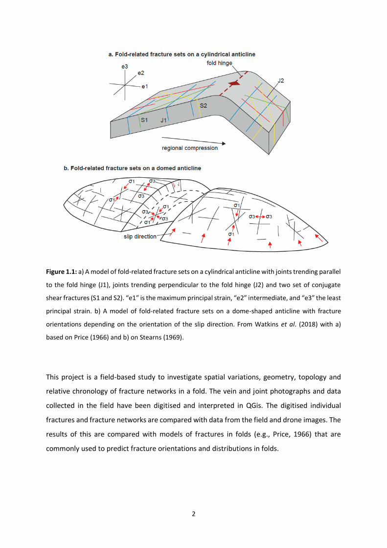
Figure 1.1: a) A model of fold-related fracture sets on a cylindrical anticline with joints trending parallel

to the fold hinge (J1), joints trending perpendicular to the fold hinge (J2) and two set of conjugate

shear fractures (S1 and S2). “e1” is the maximum principal strain, “e2” intermediate, and “e3” the least

principal strain. b) A model of fold-related fracture sets on a dome-shaped anticline with fracture

orientations depending on the orientation of the slip direction. From Watkins et al. (2018) with a)

based on Price (1966) and b) on Stearns (1969).

This project is a field-based study to investigate spatial variations, geometry, topology and

relative chronology of fracture networks in a fold. The vein and joint photographs and data

collected in the field have been digitised and interpreted in QGis. The digitised individual

fractures and fracture networks are compared with data from the field and drone images. The

results of this are compared with models of fractures in folds (e.g., Price, 1966) that are

commonly used to predict fracture orientations and distributions in folds.

3

1.2 Aims and objectives

The aim of this project is to improve the understanding of fracture patterns in folds and discuss

implications for this work for models of fractures in folds and fluid flow in the subsurface.

Fractures have been analysed from a metre-scale on a fold in Bude (The Whaleback Fold),

Cornwall, UK, using field measurements, field photographs and drone imagery.

The objectives are to:

1) Compare the fracture networks in the limbs and crest of the Whaleback, quantifying

spatial variations in geometry, topology and relative chronology around the fold.

2) To compare field observations, analysis of drone images and published models for

relationships between folds and fractures.

3) To reconstruct and interpret the timing and spatial variability of fracturing during fold

development.

4) To discuss the implications of this work for models of fractures in folds, and for fluid

flow within fractured reservoirs.

1.3 Field area

Fieldwork was undertaken on the Whaleback fold, which is located just outside the Bude

Breakwater, along the coast of northern Cornwall in South West England (Fig. 1.2).

Photographs and drone imagery were collected in the field in late June 2019. The coast of

northern Cornwall is known for contractional structures that are well-exposed in sea cliffs and

on wave-cut platforms.

4

Figure 1.2: a) Overview map with the location of the SW England region. b) Map of the SW England

region with the location of the study area along the Northern Cornwall coast. c) Overview of the study

area at Bude Breakwater beach with the dotted rectangle representing the focus area on the

Whaleback fold. a) and b) are satellite images from Google Earth Pro (2020) and c) is a drone image

from the fieldwork.

5

The main focus area on the Whaleback fold is approximately 20m long and is located at

50°49´46’’N 4°33’21’’W. The outermost bed is well-exposed and can be traced as up to

approximately 85m long using drone imagery. The fold consists of alternating beds of

sandstone and shale with networks of joints and veins, perfect for studying fractures around

folds. The outermost exposed bed in the Whaleback is a sandstone bed that is exposed across

the fold and is therefore the main focus in the fracture network analysis. The Whaleback fold

is an excellent exposure to observe and interpret fracture characteristics and differences at

various structural positions in a fold. It is an accessible and well-exposed anticlinal pericline

where different fracture types and generations occur. The fracture networks vary across the

fold and along the limbs, with the Whaleback being a good location to test published models

for the relationships between folds and fractures.

6

2 Theoretical background

This chapter aims to define the main terms used, introduce different types of fractures in rocks

and the relationships between them, and show different models that have been used to relate

fractures to folds.

2.1 Fractures

2.1.1 Fracture types

Figure 2.1: Mohr diagram of shear stress (τ) against normal effective stress (σ’N) showing the fields in

which extension (1), hybrid (2) and shear (3) fractures occur. Modified from Ramsey and Chester

(2004).

Fractures are common structures found in rocks exposed at the surface of the Earth (Bourne

and Willemse, 2001). Joints and veins are opening-mode fractures, with displacement

perpendicular to the fracture surface, while faults are shear fractures, with displacement

parallel to the fracture surface (Schultz and Fossen, 2008; Peacock et al., 2016). A joint is an

opening-mode fracture with micro- to millimetre-scale openings (Fig. 2.2a) (Peacock et al.,

7

2016). Some fractures that originate as joints can be mineralised to form veins. Some veins,

however, did not originate as joints. Faults are planar structures across which shear

displacement occur (Fig. 2.2c) (Peacock et al., 2016). Veins, joints and faults are all types of

fractures, so in this thesis the term “fracture” is only used when it is uncertain whether it is a

vein or a joint. For example, partly-filled veins are termed fractures when it is unclear whether

they are weathered veins or weathered joints (Fig. 2.2).

Figure 2.2: Photographs of different fracture types on the Whaleback fold in Bude, SW England. a)

Photograph from the northern limb showing examples of quartz-filled veins and two joints cross-

cutting the veins, with no mineral fill. b) Photograph from the southern limb showing examples of

fractures, where it is unclear what type of fractures it is. c) Photograph showing examples of faults

(dashed lines) with arrows indicating relative direction of displacement on some of them. The faults

are confined to the shale units, bounded by two massive sandstone beds.

8

2.1.2 Mechanical stratigraphy and fracture stratigraphy

Mechanical stratigraphy is defined as the mechanical properties of units, unit spacing, their

relative thicknesses and the nature of unit boundaries (Cawood and Bond, 2018). The

mechanical properties that influence the growth of opening-mode fractures include tensile

strength, fracture mechanics properties and brittleness etc. and have been used to explain

various structural patterns and features, e.g., style of folding (Laubach et al., 2009; Cawood

and Bond, 2018). Fracture stratigraphy subdivides rocks into fracture units that are based on

extent, intensity or other observed fracture features (Laubach et al., 2009). Mechanical

stratigraphy is the by-product of depositional composition and structure, including the

mechanical and chemical changes after deposition, while fracture stratigraphy reflects the

loading history (Laubach et al., 2009). These concepts are important for accurately predicting

fractures, as it can be useful to use observations and models of diagenesis to extrapolate

previous mechanical states (Laubach et al., 2009).

Fractures in layered sedimentary sequences can be classified as stratabound or non-

stratabound (Odling et al., 1999). The veins and joints observed on the Whaleback fold seem

to be largely stratabound. Stratabound fractures are confined to single beds (or groups of

beds), bounded by the bedding surfaces at the top and bottom of a layer, and therefore

restricted in size by thickness of the strata (i.e. length of the fracture measured perpendicular

to the bedding planes) (Odling et al., 1999). Non-stratabound fractures, on the other hand,

can affect two or more beds so it can exceed the size of individual beds (Odling et al., 1999).

Stratabound fractures are common in interbedded sequences of weak and strong layers, such

as sandstones and shales (Guerriero et al., 2015), and often occur at shallow crustal levels

(Odling et al., 1999). Fig. 2.2 show faults confined to the shale units bounded by massive

sandstone beds, which is a good example of mechanical stratigraphy and stratabound

fractures.

9

2.2 Fracture networks

Fracture networks are a group or system of fractures developed within the same rock mass,

which may or may not intersect (Sanderson and Nixon, 2015). Fracture networks can involve

a number of fracture sets and be described in terms of their orientation, frequency, spacing,

length and intensity (Strijker et al., 2012; Sanderson and Nixon, 2015; Peacock et al., 2016). A

number of criteria can be used to define a set, and this is further described in Section 2.2.3.

Sanderson and Nixon (2015) define frequency as the number of fractures per unit area and

fracture intensity as the total trace length per unit area (Dershowitz and Einstein, 1988). With

2-dimensional sampling the 2D intensity is defined as branch length per unit area (Sanderson

and Nixon, 2015). Fractures and fracture networks are three-dimensional structures, although

they are often interpreted as two-dimensional. In this thesis, fracture traces on exposed

bedding surfaces are interpreted, meaning the 3D fracture networks is seen and interpreted

in 2D.

2.2.1 Relationships between pairs of fractures

Peacock et al. (2018b) describe the different geometries that can characterize the

relationships between two fractures (Fig. 2.3);

• Isolated: when a fracture does not kinematically or geometrically interact with each

other. These fracture tips terminate in rock matrix, creating isolated fracture tips

(Sanderson and Nixon, 2015).

• Abutting: when a fracture links with another fracture and forms Y- or T-intersection.

This relationship is often observed with one fracture linking a pre-existing fracture at

a high angle.

• Cross-cutting: when a younger fracture crosses an older fracture, or two synchronous

fractures mutually cross-cuts each other.

10

Figure 2.3: Illustration showing examples of joints intersecting, including examples of abutting, isolated

and cross-cutting relationships that are marked with red circles.

2.2.2 Relationships between two fracture sets

Fracture networks can make up patterns based on the intersecting angle between two

fracture sets, and is commonly classified as orthogonal if two fracture sets are perpendicular

to each other and non-orthogonal if the angle is less than about 90° (Fig. 2.4) (Caputo, 1995;

Bai et al., 2002; Pluijm and Marshak, 2004). Orthogonal sets create ladder or grid patterns of

different varieties (Rives et al., 1994). Rives et al. (1994) define ladder pattern as a set of long

parallel fractures with a second set of fractures that systematically abuts the initial set (Fig.

2.4). Grid pattern is termed when two sets of fractures systematically and mutually cross-cut

each other (Fig. 2.4) (Rives et al., 1994). Conjugate relationships refers to faults where

conjugate patterns consists of two faults with opposite shear sense, but with the same angle,

generally 30°, to the maximum principal stress direction (Peacock et al., 2016). A set of

conjugate shear joints is, however, predicted to form in both limbs during folding in the Price

(1966) model. Pollard and Aydin (1988) argue that these shear joints should be termed faults,

because they would have shear displacement. A problem with “shear joints” seems to be that

they do not actually show any measurable shear, and that they appear to be termed conjugate

based on the angle they are formed at. In some cases, fracture networks have no regionally

11

consistent strike orientation, creating what is termed a polygonal pattern (Fig. 2.4) (Gray,

1986; Lonergan et al., 1998). This means that the fractures have not formed as a response to

a tectonic event and that the polygonal fractures have no systematic strike distributions

(Lonergan et al., 1998). In other cases, veins can make up a intense network of several sets or

randomly orientated veins, called a stockwork (Fig. 2.4) (Peacock et al., 2016).

Figure 2.4: Illustrations of different fracture patterns. Illustration of fluid-assisted breccia is modified

from Jébrak (1997).

In the Whaleback fold there is a spatial change from areas with some vein sets, to areas with

more intense and widely distributed vein networks. In some areas it appears to be possible to

restore the blocks with intense vein networks of host rocks to its original configurations. In

other areas, where there are patches of breccia, restoration appears to be difficult or not

possible. Jébrak (1997) describes hydrothermal breccias in terms of mechanisms, evolution

12

and geometry etc., and it appears that the breccias observed on the Whaleback are likely to

be fluid-assisted breccias (Fig. 2.4). Fluid-assisted breccias are especially common in the brittle

part of the crust and interpreted as being related to hydrothermal fluids (Jébrak, 1997). This

hypothesis is not further discussed as there is no geochemical data from the Whaleback in this

thesis.

2.2.3 Fracture sets

Fractures in a network are commonly grouped into different sets to help describe or

understand the geometries, histories, kinematics and mechanics of the fractures, and their

significance for tectonics and fluid flow. A “set” is a group or collection of related things, and

so can be defined in various ways. For instance, fracture sets can be defined by fracture type,

orientation, relative age, length or size and whether they are stratabound or non-stratabound

etc. (Peacock et al., 2018). Fracture networks can consists of many sets, where a set of

fractures may have developed during one deformation event or during a sequence of

deformation events (Peacock et al., 2018).

Dividing fractures into sets is important in this thesis, because the goal is to understand the

evolution of fractures in folds, including fractures that are formed pre-, syn- and post-folding.

In the Whaleback fold case, it is important to distinguish between veins and joints where

possible, and to understand the relative ages and the development of different fractures,

because this will help show how they relate to fold development. An aim of this thesis is to

show which sets formed before, during or after folding. The fracture sets are also used in the

comparison of models for fractures in folds, including the Price (1966) model. These models

are discussed in more detail in Section 2.4.

2.3 Topology

As stated by Peacock et al. (2016), topology describes the geometric relationships and spatial

arrangements of objects. Topology is used in this thesis to characterize the fracture networks

observed in the field and compare the properties around the Whaleback fold.

13

Figure 2.5: Fracture trace marked as black bold line with intersecting fractures (dashed lines), showing

the arrangement of nodes and branches. Branches are classified based on the nodes, where I-node is

isolated, X-node is crossing, and Y-node are abutting. The nodes are based on the fracture

relationships, where two fractures that cross-cuts each other creates an X-node in that point.

2.3.1 Node classification

Nodes are used to indicate what type of relationship it is between fractures and can therefore

be useful in the determining the relative ages between the fracture sets. Nodes are divided

into those that are isolated (I), crossing (X) and abutting (Y), and these can be used to classify

types of branches (Fig. 2.5) (Manzocchi, 2002; Sanderson and Nixon, 2015; Peacock et al.,

2016; Nyberg et al., 2018);

• I-node: where a fracture terminates as a free tip.

• X-node: where two fractures cross-cut each other to form an X pattern.

• Y-node: where one fracture abuts another fracture.

X- and Y-nodes are both “connecting nodes”, where the traces of two fractures intersect.

When a fracture extends outside of the interpretation area, the point at which the fracture

intersects the interpretation boundary is termed an edge node (E-node) (Nyberg et al., 2018).

14

Fracture networks consist of lines, nodes and branches in two-dimensions that can be used to

define orientation, length and topology (Sanderson and Nixon, 2015). One line can consist of

one or more branches, including a node at each end.

2.3.2 Branch classification

Branches are classified based on number of I-nodes and can be divided into: (1) branches with

no I-nodes; (2) branches with one I-node; (3) branches with two I-nodes (Sanderson and Nixon,

2015). These are termed doubly connected (C-C), partly connected (I-C) and isolated (I-I)

branches respectively (Fig. 2.5) (Ortega and Marrett, 2000; Sanderson and Nixon, 2015). The

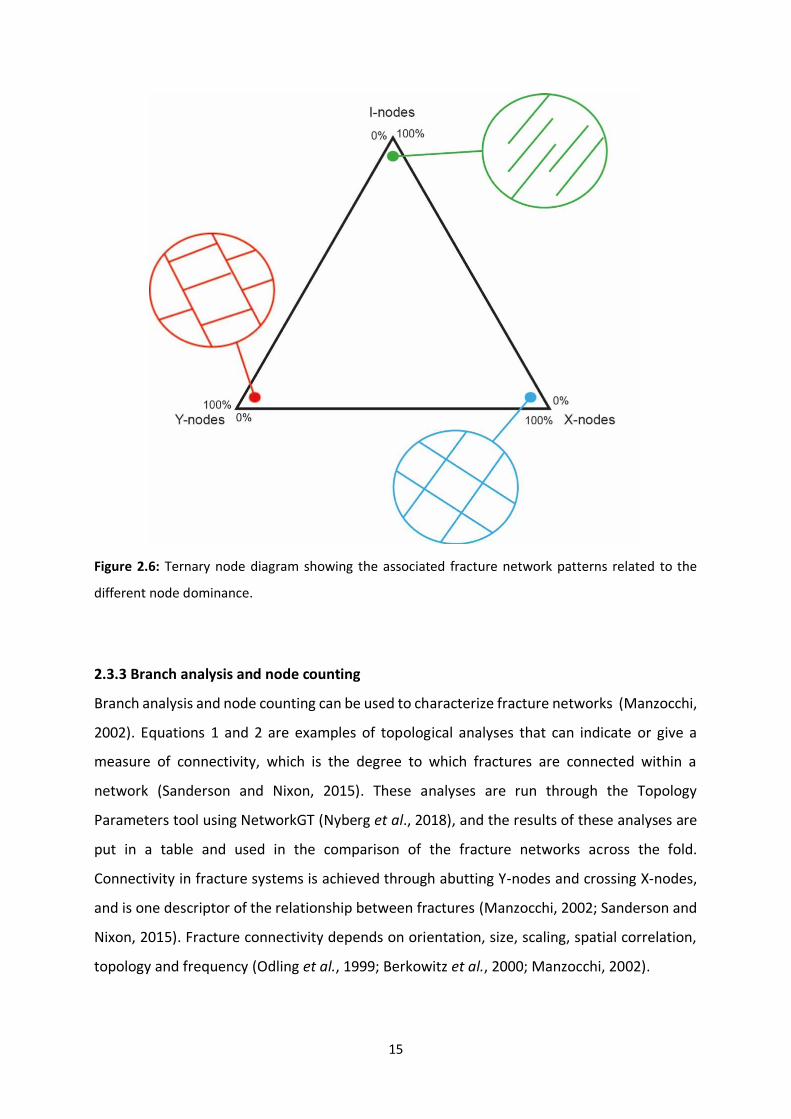
proportions of the different types of nodes and branches can be plotted in ternary diagrams

and used to interpret and compare different fracture sets and their relative ages (Fig. 2.6). A

set of fractures that consist of Y-nodes, can show I-C and/or C-C branches. This means that

they abut at least one other set of fractures and this can indicate that they are younger than

the set of fractures they abut (Fig. 2.6).

15

Figure 2.6: Ternary node diagram showing the associated fracture network patterns related to the

different node dominance.

2.3.3 Branch analysis and node counting

Branch analysis and node counting can be used to characterize fracture networks (Manzocchi,

2002). Equations 1 and 2 are examples of topological analyses that can indicate or give a

measure of connectivity, which is the degree to which fractures are connected within a

network (Sanderson and Nixon, 2015). These analyses are run through the Topology

Parameters tool using NetworkGT (Nyberg et al., 2018), and the results of these analyses are

put in a table and used in the comparison of the fracture networks across the fold.

Connectivity in fracture systems is achieved through abutting Y-nodes and crossing X-nodes,

and is one descriptor of the relationship between fractures (Manzocchi, 2002; Sanderson and

Nixon, 2015). Fracture connectivity depends on orientation, size, scaling, spatial correlation,

topology and frequency (Odling et al., 1999; Berkowitz et al., 2000; Manzocchi, 2002).

16

The ratio between the number of branches to lines is:

NB / NL = (4 – 3PI – PY) / (PI + PY) (eq. 1)

Where NB is number of branches, NL is number of lines and PI and PY represent the proportion

of I- and Y-nodes (Sanderson and Nixon, 2015). Node counting can give information about the

type of fractures, e.g., NB/NL=1 there is a dominance of isolated fractures. Node counting can

also be used to help determine the relative ages of the fracture sets, based on the observation

that younger fractures tend to abut or cross older fractures (Peacock et al., 2018). The number

of connections per branch (CB) can be derived from the number of different node types:

CB = (3NY + 4NX)/NB (eq. 2)

NY is number of Y-nodes, NX is number of X-nodes and NB number of branches (Sanderson and

Nixon, 2015). CB can only be a number between 0-2, where the higher the number the higher

the connectivity of the network is (Sanderson and Nixon, 2015).

2.4 Networks of joints and veins associated with folds

There has been a considerable amount of work devoted to understand the development of

folds and fractures and to predict fracture patterns in the subsurface, which is important for

reservoir modelling (Mapeo and Andrews, 1991; Couples et al., 1998; Cosgrove and Ameen,

2000; Fischer and Wilkerson, 2000; Jäger et al., 2008; Casini et al., 2011; Pearce et al., 2011;

Cosgrove, 2015; Li et al., 2018). Cosgrove (2015) suggests that in some cases, it is the process

of folding that generates fractures, but in the case of forced folds, the reverse is true. Various

models are used for the geometric relationship between folds and fractures (e.g., Price, 1966;

Stearns, 1969; Watkins et al., 2015), and these models tacitly or explicitly assume that

fracturing is synchronous with folding, with relatively few papers describing fractures that pre-

or post-date folding (e.g., Mapeo and Andrews, 1991; Casini et al., 2011). Some use strain or

curvature in folds to generate fracture models in reservoir engineering (e.g., Lisle, 1994, 2000;

Fischer and Wilkerson, 2000; Pearce et al., 2011). Folded upper crustal rocks usually contains

several fracture sets with different orientations and it can be difficult to link the different

fracture sets to the specific tectonic episodes (Jäger et al., 2008). Jäger et al. (2008) show that

17

the most common fracture sets related to folding of upper crustal rocks are perpendicular to

bedding and either orthogonal or parallel to the fold axes.

2.4.1 Models of fractures in folds

Various approaches are used to analyse fracture patterns within folds. Price (1966) and

Stearns (1969) are examples of conceptual models that relate fracture orientations to fold

geometry (Fig. 1.1). Others study outcrops to gain information about fracture formation and

what controls it (e.g., Wennberg et al., 2007; Watkins et al., 2015, 2018). Cosgrove (2015)

studies the various types of fold-fracture associations and the development of these, by

looking at strain distributions within the folds. Determining fracture distributions in the

subsurface can be difficult with data typically limited to core and image logs, resulting in the

use of curvature or strain within a fold to predict fracture patterns and distributions and fluid

flow (Ericsson et al., 1998; Fischer and Wilkerson, 2000; Pearce et al., 2011; Watkins et al.,

2015). These models make explicit or tactic assumptions about the geometric, mechanical and

temporal relationships between fold and fractures, that may not be correct. The Price (1966)

and Stearns (1969) are simple geometric models that assume that the fractures form in

response to stresses within the fold, assuming folding and fracturing are the same age, which

may not be correct. The Price model (1966) also discusses “shear joints”, which is an

interpretation criticised by Pollard and Aydin (1988).

2.4.2 The flexural slip mechanism

The folds in the Bude Formation is suggested to have been formed by flexural slip folding

(Ramsay, 1974; Tanner, 1989), and this have implications for the patterns of fractures within

folds, including the Whaleback. The aim is to observe what effect this has on fracture patterns

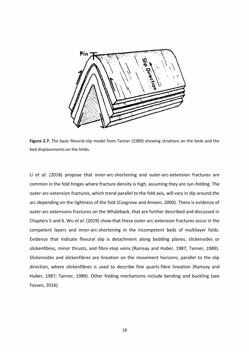
and distributions. Flexural slip is when one layer slip over another as the dip of the limb

increases in response to lateral shortening (Fig. 2.7) (Tanner, 1989). During folding, slip is

activated on only some bedding plane horizons, with deformation patterns contained within

the mechanical units based on the slip horizons (Couples et al., 1998). Couples et al. (1998)

show that these deformation patterns have been recognized in folded rocks by various

workers (e.g., Price, 1966; Stearns, 1967; Ramsay and Huber, 1987).

18

Figure 2.7: The basic flexural-slip model from Tanner (1989) showing striations on the beds and the

bed displacements on the limbs.

Li et al. (2018) propose that inner-arc-shortening and outer-arc-extension fractures are

common in the fold hinges where fracture density is high, assuming they are syn-folding. The

outer-arc-extension fractures, which trend parallel to the fold axis, will vary in dip around the

arc depending on the tightness of the fold (Cosgrove and Ameen, 2000). There is evidence of

outer-arc extensions fractures on the Whaleback, that are further described and discussed in

Chapters 5 and 6. Wu et al. (2019) show that these outer-arc-extension fractures occur in the

competent layers and inner-arc-shortening in the incompetent beds of multilayer folds.

Evidence that indicate flexural slip is detachment along bedding planes, slickensides or

slickenfibres, minor thrusts, and fibre-step veins (Ramsay and Huber, 1987; Tanner, 1989).

Slickensides and slickenfibres are lineation on the movement horizons, parallel to the slip

direction, where slickenfibres is used to describe fine quartz-fibre lineation (Ramsay and

Huber, 1987; Tanner, 1989). Other folding mechanisms include bending and buckling (see

Fossen, 2016).

19

3 Geological setting

The Whaleback fold in Bude is located of the Celtic Sea at Bude, North Cornwall in SW England.

The area shows folds well-exposed in sea cliffs and wave-cut platforms. Several studies have

been published about this area (Sanderson and Dearman, 1973; Sanderson, 1979; Whalley

and Lloyd, 1986; Lloyd and Chinnery, 2002). The Whaleback fold and the fractures exposed on

the fold may have been influenced or controlled by a series of events between deposition and

the present day. This chapter aims to describe the general tectonic evolution and the

stratigraphy of the study area.

3.1 The Carboniferous

The Bude Formation was deposited in the early Westphalian, in a foreland basin in front of

the northward-advancing Variscan deformation front (Higgs, 1991). The Formation is

approximately 1300 m thick and is discontinuously exposed between Hartland Quay and

Widemouth Bay (Higgs, 1991). Lloyd and Chinnery (2002) state that the Formation consists of

five lithologies: sandstones, siltstones, shales, marine bands (black shales) and “slump” beds.

These slump beds have been observed and described in various ways in several studies

(Freshney and Taylor, 1972; Freshney et al., 1979; Melvin, 1986; Higgs and Melvin, 1987;

Hartley, 1991), with Hartley (1991) suggesting they resulted from both slumps and debris flow.

These lithologies consist of interbedded sequences of different sandstones and shales (Fig.

3.1) (Whalley and Lloyd, 1986). Higgs (1991) propose a coarsening-up/fining-up cycle of three

facies arranged in 12321 order. Facies 1 is dark-grey fine mudstone, facies 2 is light-grey

mudstone both containing thin sandstone beds, and facies 3 is amalgamated sandstone with

thin mudstone layers. The organic content in the shales was measured using the

carbon:sulphur ratio technique by Berner and Raiswell (1984), with the results showing low

organic content (Lloyd and Chinnery, 2002).

20

Figure 3.1: Photograph of the Whaleback in profile, showing the different lithologies observed with a

massive sandstone bed as the uppermost and outermost bed and with alternating shales underneath.

Loading structures are observed within the shale units, indicating the way up.

Two main depositional models have been proposed for The Bude Formation: 1) shallow lake

floor with turbidites being fed from rivers, based on sedimentary structures indicating wave-

21

influence (Higgs and Melvin, 1987; Higgs, 1991, 1994, 1998); and 2) deep sea fan (Melvin,

1986; Higgs and Melvin, 1987; Burne, 1995, 1998). There is a general agreement, however,

that: 1) the presence of freshwater fossils indicates deposition in brackish water with

occasional seawater incursions (Goldring, 1971; Freshney and Taylor, 1972; Burne, 1973; Lloyd

and Chinnery, 2002) and 2) that the Bude Formation was deposited away from the shore,

based both on the presence of turbidite beds and on the lack of evidence for emergence

(Reading, 1963; Goldring, 1971; Melvin, 1986). The underlying Crackington Formation is

marine but contains brackish intervals (Higgs, 1991). Together with the Bude Formation, the

two formations show a progression from open sea to isolation. Some fossil bands are marine

and represents maximum flooding surfaces, reflecting the marine incursions that forced the

lake to deepen as sea-level rose, turning the water from brackish to marine (Freshney et al.,

1979; Higgs, 2004). Higgs (2004) suggests that this was controlled by glacioeustatic variations,

with a eustatic fall forcing the lake down to sill level and turning the lake water fresh.

The Bude and Crackington formations are part of the Culm Synclinorium in the Culm Basin

(Sanderson, 1979). The Culm Basin initiated in the Upper Devonian as an extensional basin

during continental rifting (Leveridge and Hartley, 2003). Sedimentation was interrupted by a

series of tectonic events in Early Tertiary and mild basin inversion during the Oligo-Miocene

(Hecht, 1992).

3.2 The Variscan Orogeny

The Variscan Orogeny took place over a period of ~100 million years during the Late

Palaeozoic, with the main contraction in SW England occurring towards the end of the

Carboniferous (Hecht, 1992; Leveridge and Hartley, 2003). It was a result of the collision

between Laurentia and Gondwana, which created the supercontinent Pangea and led to the

formation of the Variscan mountain belt (Hecht, 1992; Kroner and Romer, 2013). NW-SE

striking veins indicate NW-SE contraction and NE-SW extension prior to folding (Jackson,

1991). This is consistent with an E-W dextral shear (Sanderson and Dearman, 1973).

22

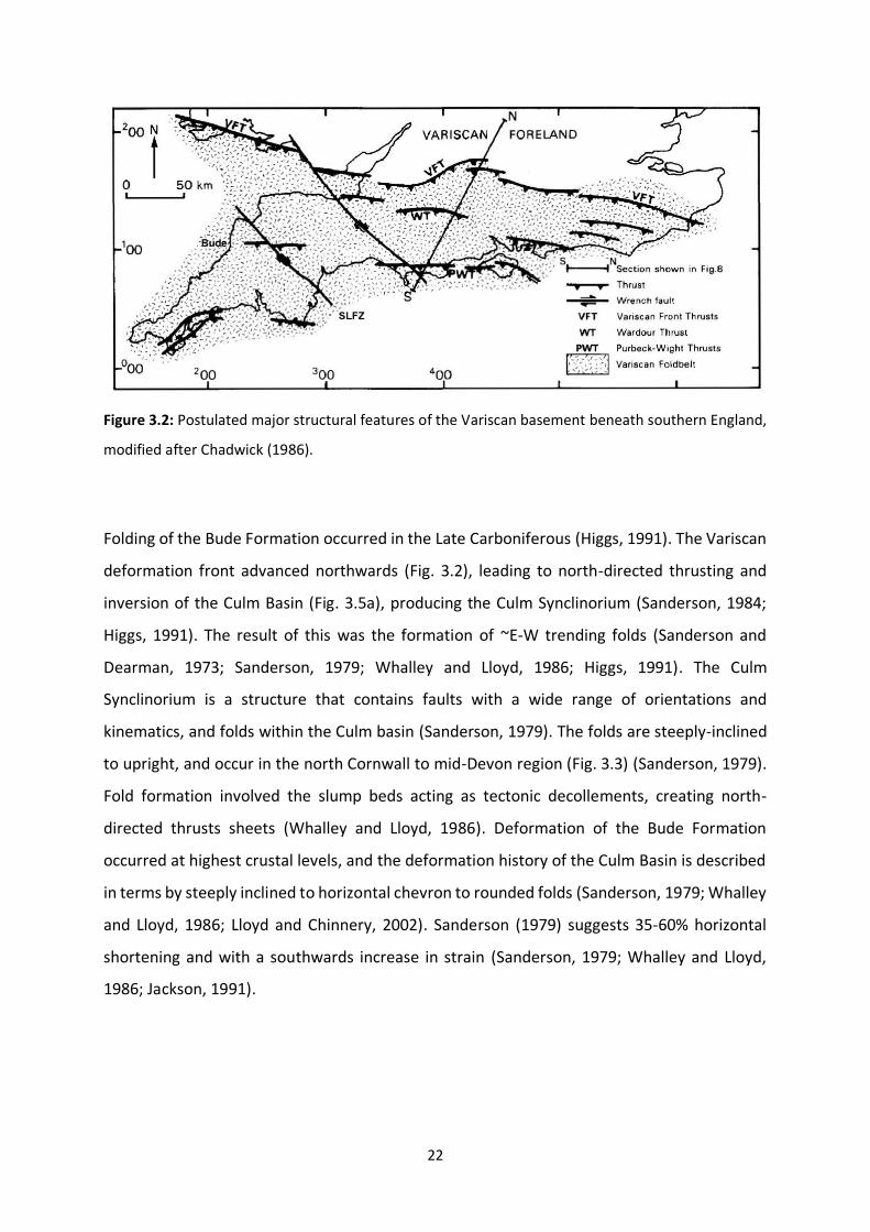
Figure 3.2: Postulated major structural features of the Variscan basement beneath southern England,

modified after Chadwick (1986).

Folding of the Bude Formation occurred in the Late Carboniferous (Higgs, 1991). The Variscan

deformation front advanced northwards (Fig. 3.2), leading to north-directed thrusting and

inversion of the Culm Basin (Fig. 3.5a), producing the Culm Synclinorium (Sanderson, 1984;

Higgs, 1991). The result of this was the formation of ~E-W trending folds (Sanderson and

Dearman, 1973; Sanderson, 1979; Whalley and Lloyd, 1986; Higgs, 1991). The Culm

Synclinorium is a structure that contains faults with a wide range of orientations and

kinematics, and folds within the Culm basin (Sanderson, 1979). The folds are steeply-inclined

to upright, and occur in the north Cornwall to mid-Devon region (Fig. 3.3) (Sanderson, 1979).

Fold formation involved the slump beds acting as tectonic decollements, creating north-

directed thrusts sheets (Whalley and Lloyd, 1986). Deformation of the Bude Formation

occurred at highest crustal levels, and the deformation history of the Culm Basin is described

in terms by steeply inclined to horizontal chevron to rounded folds (Sanderson, 1979; Whalley

and Lloyd, 1986; Lloyd and Chinnery, 2002). Sanderson (1979) suggests 35-60% horizontal

shortening and with a southwards increase in strain (Sanderson, 1979; Whalley and Lloyd,

1986; Jackson, 1991).

23

Figure 3.3: Map of southwest England showing dips of axial planes of early folds in Devonian and

Carboniferous rocks. Denser shading indicates steeper axial planes and dip symbols indicating general

attitude of fold axial planes. Figure from Sanderson (1979).

The shale and sandstone of the Bude Formation show different mechanical behaviours during

folding. Cosgrove (2015) shows that the sandstones are likely to have been dominated by

tangential longitudinal strain and the shales folded by flexural slip. Lloyd and Chinnery (2002)

state that sandstone controls the overall deformation, but that most of the strain

accommodation occurs within the shale. Therefore, the large-scale deformation may tend to

be controlled by multilayer-parallel geometry (Lloyd and Chinnery, 2002). As the multilayers

are folded, extensional fractures develops in the outer arc of the sandstone beds (Cosgrove,

2015).

Later stages of deformation were dominated by south-directed shearing related to back-

thrusting associated with the continued north-advancing Variscan deformation front (Fig. 3.4)

24

(Whalley and Lloyd, 1986). This led to modification of the pre-existing structures, including

modification of existing low angle normal faults and formation of new fold closures that

resulted in folding of earlier cleavage (Sanderson, 1979; Whalley and Lloyd, 1986). Whalley

and Lloyd (1986) also propose that the shearing modified the N-directed thrust structures and

the folds to that extent that the effects of shearing are the dominant structures (Fig. 3.4).

Figure 3.4: Photograph of the Whaleback fold in profile, showing the uppermost part of the northern

limb and hinge of the fold. Thrust planes are marked with a red dashed line and are south directed.

These are relatively minor thrusts and are a good example of structures associated with fold and thrust

belts.

Sanderson (1979) suggests that the increased development of quartz veins (in time and space)

indicate increased deformation by pressure solution in north Cornwall. A strike-slip fault zone,

the Sticklepath-Lustleigh, was formed in the Culm basin during the Late Variscan (Fig. 3.2)

(Holloway and Chadwick, 1986; Van Hoorn, 1987). The strike-slip movement was dextral

during the Variscan and reactivated in Early-Mid Paleogene (Holloway and Chadwick, 1986).

25

Figure 3.5: Maps showing the evolution of stresses in southern England since the Variscan Orogeny:

(a) Variscan N-S contraction; (b) Permian and Mesozoic N-S extension; (c) Alpine N-S contraction; (d)

Late-Alpine strike-slip; (e) Post-Alpine NE-SW extension. σ1 = maximum compressive stress, σ2 =

intermediate compressive stress, σ3 = least compressive stress, σH = maximum horizontal. Figure from

Peacock (2009).

26

3.3 Permian and Mesozoic basin development

During the Early Permian to Late Jurassic-Early Cretaceous, SW England experienced N-S

extension (Fig. 3.5b) as a result of the Variscan orogenic collapse and the development of

Mesozoic basins, including the Bristol Channel Basin (Shackleton et al., 1982; Van Hoorn, 1987;

Peacock, 2009). The extension led to rapid subsidence, the formation of normal faults in south

Cornwall, reactivation of Variscan thrusts and reactivation of the Sticklepath-Lustleigh fault in

a sinistral sense (Chadwick, 1986; Holloway and Chadwick, 1986; Van Hoorn, 1987; Peacock,

2009).

3.4 The Cenozoic

Areas adjacent to the North Atlantic margin were uplifted during the Palaeocene, including

the British Isles, where Palaeocene sediments are rare onshore (Dore et al., 1999). This uplift

has been attributed to the proto-Iceland plume (White, 1988; White and McKenzie, 1989). N-

S contraction in southern England during the Paleogene was related to the Alpine Orogeny

(Fig. 3.5c), and includes basin inversion with a phase of NE-SW trending sinistral and NW-SE

trending dextral strike-slip (Fig. 3.5d) (Dart et al., 1995; Peacock and Sanderson, 1999).

Hancock and Engelder (1989) show that in situ stress measurements indicate that the

maximum horizontal stress is commonly oriented northwest-southeast (Fig. 3.5e). Peacock

(2009) state that the maximum horizontal stress was oriented NW-SE through the latter part

of the Cenozoic. Holloway and Chadwick (1986) suggest that dextral movements on the

Sticklepath-Lustleigh fault zone are related to contractional tectonic episodes, while the

sinistral movements may have been associated with Early Cenozoic extension. These inversion

structures are not observed on the Whaleback, but the fractures observed on the Whaleback

fold may be related to the Alpine stress system. Rawnsley et al. (1998) connects joints

observed in the Bristol Channel Basin to five phases during the reduction of the Alpine stress.

The Atlantic margin experienced regional uplift during the Neogene that led to erosion and

shaping of the present-day distribution of landmasses (Dore et al., 1999).

27

4 Methods

This chapter describes the methods used for collecting data and digitisation of fractures,

identifying fracture sets and determining the relative chronology. The implications related to

the digitisation and interpretation are discussed, and a qualitative description of the

exposures is given. Fig. 4.1 show a simplified workflow of the work done.

28

Figure 4.1: Simplified workflow for the work done from fieldwork to digitising and 3D model. This study

combines observations from fieldwork and digital imaging techniques to compare fracture

characteristics, determine the relative chronology and create models for the relationships between

the fold and fractures.

4.1 Data collection and digitising

4.1.1 Field work and data collection

Field data were collected from specific locations on the Whaleback fold using a camera and

drones. Fig. 4.2 show examples of the altitudes at which the drone images of the Whaleback

fold were taken. The locations are chosen based on the structural position on the fold and

quality of exposed bedding surfaces. Each location has been described, including

measurements of bed dips and a classification of fracture sets based on; (a) fracture type, (b)

abutting or cross-cutting relationships; (c) orientations, and; (d) lengths (see Section 4.2). The

outermost exposed sandstone bed is the best exposed bed on the Whaleback fold and is

therefore the main focus bed in this thesis (Fig. 4.3). There are some locations in other beds,

and these are discussed further in Chapters 5 and 6.

29

Figure 4.2: Drone images of the Whaleback fold taken at three different altitudes. a) 120m, b) 50m,

and c) 10m. The Whaleback fold and the fracture patterns are analysed using drone images taken at

different altitudes, with it here showing how the fracture pattern changes at the specific altitudes.

30

The field photographs from the different locations were taken approximately perpendicular

to bedding, imported and georeferenced in QGis. Fractures were digitised and divided into

separate linestrings based on the different fracture types e.g., veins and joints. A linestring, or

polyline, is a linear feature made up of a sequence of points and the line segments connecting

them (Nyberg et al., 2018). Distinguishing between veins and joints can be difficult because it

is in some cases unclear if a fracture is a vein filled by a brown material or is a joint around

which brown weathering has occurred. The term fracture is used where it is not clear if the

fracture is a vein or a joint. Figure 4.3 shows a drone image of the Whaleback fold and the

field locations. Locations 1-5 are on the northern limb, Locations 6-8 are on the southern limb,

and Locations 9-10 are at the crest.

Figure 4.3: Photograph of the Whaleback fold with the different locations labelled across the fold, on

the outermost exposed sandstone bed. Locations 1 to 5 are located on the northern limb, Locations 6

to 8 are on the southern limb and Locations 9 to 10 are at the crest. Locations 1, 6 and 9 are discussed

in most detail because they have the best quality exposure.

31

The orthomosaic was generated using photographs taken from a DJI Phantom 4, from a height

of approximately 10 m, using Agisoft Metashape with a pixel size of 4.4 mm. The beds and

fractures were unfolded to observe if fractures on different limbs have the same orientation

after unfolding, which may suggest they pre-date folding. The bed measurements and fracture

orientations were plotted as planes in a stereonet using a data program called Stereonet

v.11.2.2 and unfolded using the “Unfold bedding…” tool (Allmendinger et al., 2013; Cardozo

and Allmendinger, 2013). The axial plane was created using “Axial Plane Finder…”, measuring

both strike and dip, and trend and plunge measurements for the axial plane and the interlimb

angle.

4.1.2 Digitising fractures in QGis

Fractures were digitised in QGis and their geometries and topologies were analysed using

NetworkGT (Nyberg et al., 2018). NetworkGT is a tool for the analysis of nodes and branches,

with nodes being classified as X-, Y- and I-nodes (Nyberg et al., 2018). E-nodes, or edge-nodes,

represent the point at which branches are cut by a polygon and that terminates somewhere

outside the interpretation area (Nyberg et al., 2018). The area within the polygon is the

interpretation area, with the edges of the polygon marking the interpretation boundary at

which E-nodes are created. Branches were digitised as polylines and classified based on node

types; C-C, I-C or I-I branches, where C represent a connecting node (Nyberg et al., 2018).

Branches that terminate outside the interpretation area, with E-nodes, were classified as U-

branches (Nyberg et al., 2018). For the digitising of nodes and branches to be accurate it is

important to “snap” the digitised polylines. If a joint abuts a vein, the “snapping” function will

snap the digitised joint exactly where it abuts the vein, creating a Y-node. In contrast, without

the “snapping” function the joint are classified as an isolated node, creating a consequential

error in the interpretation. The use of snapping options in QGis is important, because it

enables topological analyses and includes the relationships between fractures that can

indicate the relative ages. This is discussed further in Section 6.1.4.

32

After the branches and nodes have been created in NetworkGT, the networks were analysed

to determine topological parameters. The topological parameters are created through the

Topology Parameters tool and show the results in a table of topological features within the

fracture network, including number of nodes and branches, the number of the different kinds

of nodes and branches, connectivity and average length, etc.

4.2 Identifying fracture sets

4.2.1 Fracture relationships and relative ages

The relative ages of any two linked fractures are mainly based on mineralisation, kinematics

and their abutting and crossing relationships (e.g., Cosgrove and Ameen, 2000; McGinnis et

al., 2015; Peacock et al., 2018). A younger vein will abut or cross an older vein, while a younger

joint will typically abut an older joint (Fig. 4.4). Crossing relations of veins can be identified if

those veins have different mineral compositions or fibre orientations, although it is difficult to

identify such relationships on the Whaleback fold. It is common to see joints cutting veins, but

it is unusual to see veins cutting joints. This is because veins pre-date or are synchronous with

the mineralisation events, while joints post-date mineralisation. Mineralisation can therefore

be used to determine the relative ages of the different fractures.

Figure 4.4: Schematic illustration showing the different relationships between a) fractures and joints

and b) veins. a) Fracture B abuts fracture A, then fracture A is older than fracture B. Fracture C cross

33

fracture A, making the relative age relationship between them difficult to determine. b) Vein B cuts

across vein A, then vein B is younger than vein A.

4.2.2 Aims of dividing fractures into sets

Fractures are divided into sets based on the fracture type, orientation, length and abutting or

crossing relationships with the aims of; (1) comparing different locations, (2) determining age

relationships and (3) comparing with existing models for fractures within a fold. The fracture

networks in the Whaleback fold are divided into veins and joints, or fractures when the criteria

for either fracture type are not met. Based on the fracture type, sets are termed as V = veins,

J = joints and A = fractures (undefined fracture type). The fractures with unclear origin are

termed “A” to not be confused with faults. The sets are further divided based on orientation,

length and abutting and crossing relationships, and termed with numbers to separate them,

e.g., J1, J2 etc. The numbers are assigned randomly and not correlated with the relative ages,

meaning J2 may or may not be younger than J1. The relationships between the fracture sets

are discussed in Sections 5.2 and 5.3.

4.2.3 Criteria for identifying fracture sets

Several criteria have been used to divide fractures into different sets (see Section 5.2):

1. Distinguish between veins and joints where possible, or “fracture” if it is not possible

to be more specific about the fracture type. The different set of veins are termed and

numbered V1, V2, etc. and labelled with a “N” for the veins on the northern limb, “S”

on the southern limb and “C” at the crest.

2. The orientations and relative age relationships of veins are used to define sets.

3. Joint sets are defined based on:

- Whether or not they follow pre-existing veins

- Orientation

- Length

- Whether they abut other joints or abut veins

34

The fractures were first divided into sets individually on the northern limb (Location 1), the

southern limb (Location 6) and at the crest (Location 9) (Fig. 4.3). After the fracture sets were

identified at each of those three locations, they were correlated together where suitable

(Section 5.3). The different set of veins are termed and numbered V1, V2, etc. and labelled

with a “N” for the veins on the northern limb, “S” on the southern limb and “C” at the crest.

The joints are termed and numbered J1, J2, etc. and labelled with a “N” for the joints on the

northern limb, “S” on the southern limb and “C” at the crest. The fractures that is unclear

whether originated as veins or joints are termed A1, A2, etc. and also labelled with “N”, “S”

and “C” based on location. These fractures are mainly divided into sets based on orientation

and abutting and crossing relationships. Orientations have been measured in the field and by

using the 3D model of the Whaleback fold in Lime, using the “right-hand rule” where a bed

that dips to the north, strikes to the west. The relationships between the different fracture

types and sets were analysed using NetworkGT and by studying photographs.

35

5 Results

This chapter summarises the observations and interpretations from the fieldwork and from

the digitisation of photographs. Qualitative observations from the fieldwork are used to

describe the exposed surfaces, as well as characteristics and variations of the fractures across

the fold. The fracture sets and networks on both limbs and at the crest of the fold are

described and compared. The relative ages of the fractures are presented.

5.1 Qualitative description of the exposure and the fractures

The Whaleback is a periclinal fold that strike ENE-WSW (Dubey and Cobbold, 1977) and

plunges in two directions, with an average interlimb angle of 73° (Fig. 5.1). The fieldwork was

focused on the best-exposed areas of the Whaleback, which is where the fold plunges at 6°

towards 074°. The ENE-WSW strike of the Whaleback is different from the more typical E-W

trend in the region (Jackson, 1991). The fold is asymmetric, with a shallower dipping southern

limb and steeper dipping northern limb (Fig. 5.1). The limbs and crest are described in terms

of quality of the exposure and fractures.

36

Figure 5.1: Base map of the Whaleback fold with the different locations and their orientations marked

on. Bed one, marked in yellow, is the outermost exposed sandstone bed, that is 75-85 cm thick. This

bed is exposed across the fold and makes an excellent case for studying fractures in a fold. The other

beds are highlighted to illustrate the shape and distribution of the beds across the fold. Some joints

can be traced across the fold and are marked with dashed lines of green and red, while the dashed

blue line is the hinge line.

5.1.1 Northern limb (Locations 1-5)

The northern limb of the Whaleback anticline dips at 37°-44° towards the north (Fig. 5.1).

Wave erosion has given the rocks in the lower part of the limb a more “polished” appearance

than the more weathered crest (Fig 5.2). This polished effect, along the lowermost part of the

limb, makes the white-filled veins stand out and the interpretation of the fracture patterns

easier than elsewhere on the fold. Veins in this area in North Cornwall have been described

as quartz-carbonate veins (Beach, 1977; Jackson, 1991). The colour of the surface changes

from light grey in the lowermost part to darker and browner towards the crest (Fig. 5.2). In

the most eastern part of the northern limb, the veins have a wide range of orientations and

abutting and crossing relationships. These veins make up a chaotic network with a wide range

of orientations and joints cross-cutting them. Westwards on the limb, the veins develop into

a more systematic network with a more limited range of orientations than observed to the

east. The exposed surface of the limb at Locations 1 to 3 is from 3-6m high and Locations 4 to

5 is 6-7m high, from beach to the crest. The limb decreases in height towards the east as the

Whaleback plunges towards the ENE (Figs. 5.1 and 5.2).

37

Figure 5.2: Photograph of the polished appearance of the northern limb, showing how the colour of

the exposure varies from beach to crest, at Location 1, reflecting different amounts of weathering.

5.1.2 Southern limb (Locations 6-8)

The southern limb of the Whaleback fold has a shallower dip than the northern limb, being

from 29°-39° to the south (Fig. 5.1). It is harder to interpret joints and veins on the southern

limb than on the northern limb, because the exposure is more weathered (Fig. 5.3). This limb

is more sheltered from wave erosion than the northern limb, so the surface quality is poorer,

with several circular erosional features that make the analysis of the fracture networks

difficult. The upper part of the southern limb is most badly weathered, with the lowermost

third of the exposed surface being the most suitable for fracture network analysis. The degree

of weathering also varies along the limb on the lowermost part, with the most eastern part

being of best quality with increasing weathering westwards (Fig. 5.3). It is also more difficult

to distinguish between joints and veins on the southern limb than on the northern limb. Most

of the fractures on the lowermost part of the southern limb appear to be either veins filled

with a brown material or joints surrounded by a zone of alteration, with the exception of a

38

few white quartz-carbonate filled veins. The fracture network appears to be more systematic

on the southern limb, than on the northern limb, with more crossing relationships and limited

range of orientations. The variations in the fracture networks on the limbs may be a result of

weathering (Fig. 5.3), making it more difficult to observe and interpret fractures westwards

on the limb.

Figure 5.3: Photograph of the southern limb showing how the quality of the exposed surface varies

along the limb, pointing to the west. The lower part of the limb is most polished to the east, with

increasing weathering towards the west.

The most eastern part of the southern limb is more undulating than the polished surfaces on

the northern limb. At this location, there are purple spots around the brown-filled fractures.

These purple spots indicate alteration of the sandstone, possibly iron reduction, which is also

observed further west on the limb as weaker traces of alteration. Furthest east on the

Whaleback, the southern limb curves slightly towards the NE (Fig. 5.1). This part of the

southern limb is also more gently-dipping than the rest of the southern limb, with an

39

undulating surface with purple alteration spots (Fig. 5.1). The height of the limb at Locations

6 to 8 is 4-5m, decreasing as the fold plunges to the ENE (Fig. 5.3).

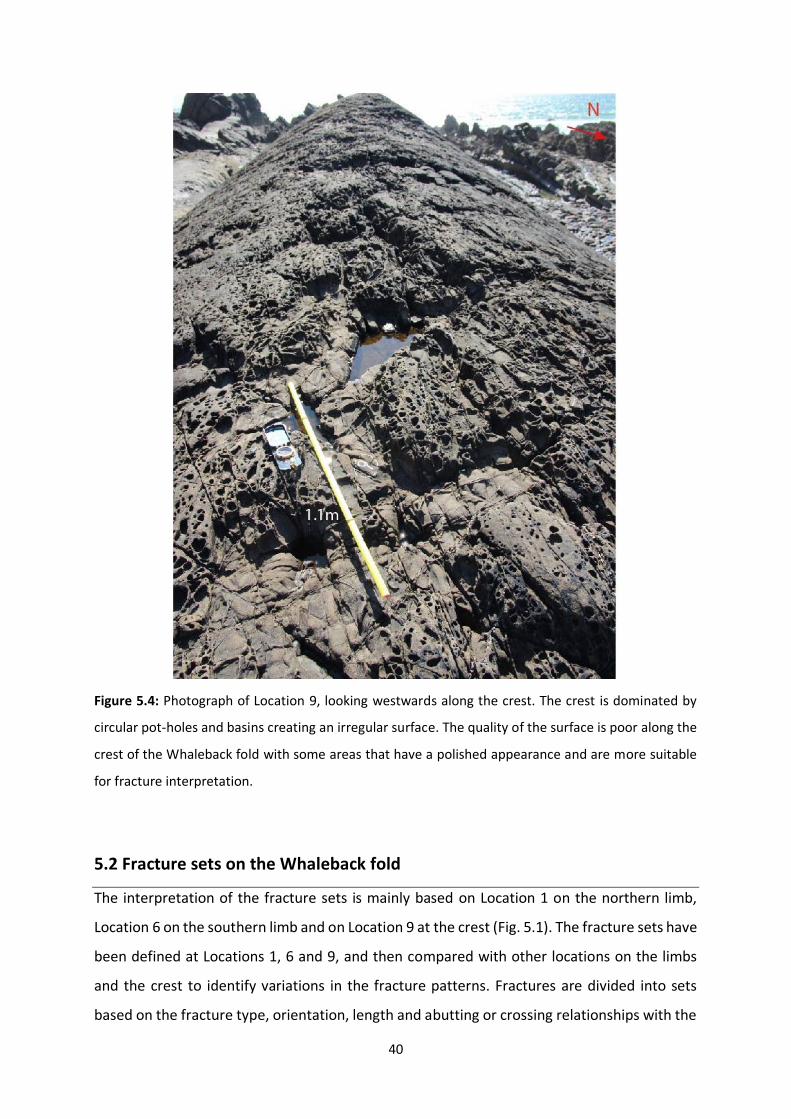
5.1.3 Crest (Locations 9-10)

The sandstone bedding plane that forms the crest of the Whaleback fold shows circular pot-

holes, up to a few centimetres deep and wide, and with several depressions with diameters

over 30-70 cm. The surface is heavily weathered and eroded, with fractures that appear to be

unfilled that may be joints or weathered-out veins (Fig. 5.4). The different fracture types are

reasonably well-exposed at Location 10, with less weathering than the surrounding areas,

while Location 9 is more weathered. The variations in surface quality along the crest make it

difficult to interpret and digitise fractures from photographs of the uneven surface. The

relationships between the fractures are also difficult to determine because of the erosional

features and weathering.

40

Figure 5.4: Photograph of Location 9, looking westwards along the crest. The crest is dominated by

circular pot-holes and basins creating an irregular surface. The quality of the surface is poor along the

crest of the Whaleback fold with some areas that have a polished appearance and are more suitable

for fracture interpretation.

5.2 Fracture sets on the Whaleback fold

The interpretation of the fracture sets is mainly based on Location 1 on the northern limb,

Location 6 on the southern limb and on Location 9 at the crest (Fig. 5.1). The fracture sets have

been defined at Locations 1, 6 and 9, and then compared with other locations on the limbs

and the crest to identify variations in the fracture patterns. Fractures are divided into sets

based on the fracture type, orientation, length and abutting or crossing relationships with the

41

aims of; (1) comparing different locations, (2) determining age relationships and (3) comparing

with existing models for fractures within a fold. The characteristics of the fracture sets are

described along the limbs and at the crest in terms of geometry and topology. Some fracture

sets can be correlated together by tracing them across the fold, while others show similar

orientations, spacing and abutting and cross-cutting relationships that can suggest they are

the same set. These sets are termed the same in both limbs and at the crest, including a “N”,

“S” or “C” to indicate where on the fold they are observed (e.g., set A2 is listed as A2N on the

northern limb, A2S on the southern limb and A2C at the crest) (Fig. 5.5). Some sets are only

observed at the crest and do not appear to be the same set of fractures observed at the limbs.

These sets are not termed with the same number as any of the other fractures sets and

indicated with a “C”. For example, J3 are only observed in the crest and termed with a “C” and

do not correspond to the joint sets J1 and J2 observed on both limbs. Set J1 is, however,

observed on both limbs and therefore termed J1N and J1S. Each set is described in terms of

fracture type, orientation, length, measured spacing, abutting and crossing relationship and

distribution. All the veins are most visible and prominent on the lowermost exposed part of

the limbs and the polished areas at the crest, with decreasing visibility towards the upper part

of the limb as weathering increases (Figs. 5.5 and 5.8).

5.2.1. Northern limb

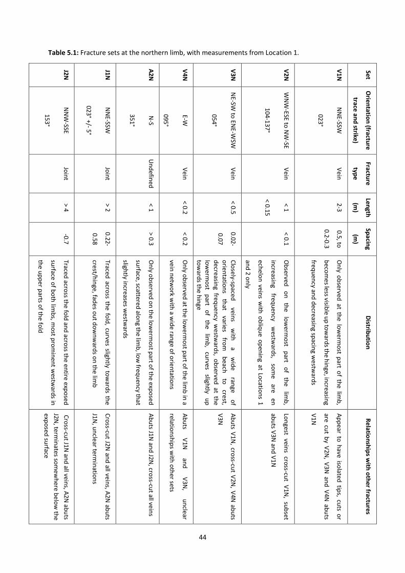
Seven fracture sets have been identified on the northern limb as either veins or joints (Table

5.1, Fig. 5.5). All the veins in this limb are completely filled with white quartz-carbonate and

easily distinguished from the joints. V1N strikes parallel to the J1N, but are only observed in

the lowermost part of the exposed surface, whereas J1N is only observed in the uppermost

part of the limb furthest east (Fig. 5.5). The correlation of V1N and J1N is therefore difficult.

The most numerous veins observed in this limb is V3N (Fig. 5.6). These veins vary in strike,

from striking approximately 040° at the lowermost part of the exposed surface to 058° in the

upper part (Table 5.1). Like V3N, J1N also curves towards the hinge of the fold (Table 5.1). V2N

both cross-cut and abut V1N perpendicular, creating a ladder and grid pattern (Table 5.1). The

longest veins of the V2N set appears to cross-cut V1N, while the veins that abut V1N represent

the shortest veins (Fig. 5.5). The en echelon veins of V2N only occur on the lowermost part of

the exposed surface (Table 5.1). These en echelon veins strike parallel with V2N and are

42

classified as the same set and are only observed within a relatively small area at the lowermost

part of the exposure at Locations 1 and 2 (Fig. 5.5).

The different sets of joints are observed along the northern limb but less visible in the

lowermost part where the surface quality is better compared to the upper part. J1N is only

observed in the upper half of the exposed surface and fades out towards the lower part, while

J2N are in more cases than J1 observed from the upper to the lower parts (Fig. 5.5). This results

in there being few cases where the relationship between the joint sets can be observed, which

makes their relative ages hard to determine. Figure 5.7 show that J1N tend to be the longest

joints, which may only be the case at Location 1, where J2N are less visible compared to the

locations further west. A2N is observed as partly-filled veins in a few cases along the limb and

as joints in most cases, so therefore termed “fractures”. A2N fractures are only observed in

the lowermost part of the exposed limb (Table 5.1), where their abutting relationships to the

joints indicates that they are the youngest set.

43

Figure 5.5: a) Illustration of the fracture sets at the northern limb, Location 1. b) Photograph of

Location 1 with the fracture sets marked on. Both figures show the relationship between the fracture

sets and where the different sets are observed at the exposed surface.

44

Table 5.1: Fracture sets at the northern limb, with measurements from Location 1.

J2N

J1N

A2N

V4N

V3N

V2N

V1N

Set

NN

W-SSE

153°

NN

E-SSW

023° +/- 5°

N-S

351°

E-W

095°

NE-SW

to EN

E-W

SW

054°

WN

W-ESE

to N

W-SE

104-137°

NN

E-SSW

023°

Orien

tatio

n (fractu

re

trace and

strike)

Join

t

Join

t

Un

defin

ed

Vein

Vein

Vein

Vein

Fracture

type

> 4

> 2

< 1

< 0.2

< 0.5

< 1

< 0.15

2-3

Len

gth

(m)

-0.7

0.22-

0.58

> 0.3

< 0.2

0.02-

0.07

< 0.1

0.5, to

0.2-0.3

Spacin

g

(m)

Traced

across th

e fold

and

across th

e entire exp

osed

surface

of b

oth

limb

s, mo

st pro

min

ent w

estward

s in

the u

pp

er parts o

f the fo

ld

Traced

across th

e fold

, curves sligh

tly tow

ards th

e

crest/h

inge, fad

es ou

t do

wn

ward

s on

the lim

b

On

ly ob

served o

n th

e low

ermo

st part o

f the exp

osed

surface

, scattered alo

ng th

e limb

, low

frequ

ency th

at

slightly in

creases westw

ards

On

ly ob

served at th

e low

ermo

st part o

f the lim

b in

a

vein n

etwo

rk with

a wid

e range

of o

rientatio

ns

Clo

sely-space

d

veins

with

a

wid

e ran

ge o

f

orien

tation

s th

at varies

from

b

each

to

crest,

decreasin

g frequ

ency w

estward

s, ob

served at th

e

low

ermo

st p

art o

f th

e lim

b,

curves

slightly

up

tow

ards th

e hin

ge

Ob

served

on

th

e lo

werm

ost

part

of

the

limb

,

increasin

g freq

uen

cy w

estward

s, so

me

are en

echelo

n vein

s with

ob

liqu

e o

pen

ing at Lo

cation

s 1

and

2 on

ly

On

ly ob

served at th

e low

ermo

st part o

f the lim

b,

beco

mes less visib

le up

tow

ards th

e hin

ge, increasin

g

frequ

ency an

d d

ecreasing sp

acing w

estward

s

Distrib

utio

n

Cro

ss-cut J1N

and

all veins, A

2N ab

uts

J2N, term

inates so

mew

here b

elow

the

expo

sed su

rface

Cro

ss-cut J2N

and

all veins, A

2N ab

uts

J1N, u

nclear term

inatio

ns

Ab

uts J1N

and

J2N, cro

ss-cut all vein

s

Ab

uts

V1N

an

d

V3N

, u

nclear

relation

ship

s with

oth

er sets

Ab

uts V

1N, cro

ss-cut V

2N, V

4N ab

uts

V3N

Lon

gest

veins

cross-cu

t V

1N, su

bset

abu

ts V3N

and

V1N

Ap

pear to

have iso

lated tip

s, cuts o

r

are cut b

y V2N

, V3N

and

V4N

abu

ts

V1N

Relatio

nsh

ips w

ith o

ther fractu

res

45

Figure 5.6: Graphs with cumulative plots of the veins at Location 1, on the northern limb. a) Cumulative

length versus orientation, showing the orientations of the longest veins with the dominant being at

043°-082° degrees NE-ENE. b) The cumulative number versus orientation showing a straighter line than

for the cumulative length but with the same orientation dominating. Both graphs show that V3N is the

0

10

20

30

40

50

60

70

0 20 40 60 80 100 120 140 160 180

Cu

mu

lati

ve le

ngt

h(m

)

Orientation

Location 1, veinsa)

0

100

200

300

400

500

600

700

800

0 20 40 60 80 100 120 140 160 180

Cu

mu

lati

ve n

um

ber

Orientation

Location 1, veinsb)

V3N

V3N

46

dominating set based on the length and number of veins. The area of Location 1 is 1.4673m2 with

bedding striking at 260° and dipping at 42°. 940 fracture traces are digitised and measured with 834 of

them being veins.

0

2

4

6

8

10

12

14

0 20 40 60 80 100 120 140 160 180

Cu

mu

lati

ve le

ngt

h(m

)

Orientation

Location 1, joints

0

20

40

60

80

100

0 20 40 60 80 100 120 140 160 180

Cu

mu

lati

ve n

um

ber

Orientation

Location 1, joints

J1N

J1N

a)

b)

47

Figure 5.7: Graphs with cumulative plots of the joints at Location 1, on the northern limb. a) Cumulative

length versus orientation, showing the orientation of the joints that tend to be longest. b) The

cumulative number versus orientation showing a slightly straighter line with the steepest slopes

showing the dominant orientation. Both graphs show that orientation of joints with the set striking at

029°-048° (NNE-NE) dominates, but this is clearer when they are length weighted. The area of Location.

1 is 1.4673m2, with bedding striking at 260° and dipping at 42° to the north. 940 lines are digitised and

measured with 106 of them classified as joints.

5.2.2 Southern limb

Seven fracture sets are identified on the southern limb (Table 5.2, Figs. 5.8-5.10). Dividing

fractures into sets is more difficult on the southern limb compared to the northern limb. This

is because of weathering, so that there is only one set that can be classified with certainty as

veins, with the majority of the fractures showing brown material that may be either

weathered vein-fill or alteration around joints (Fig. 5.8). These veins (V1S) are only observed

at the lowermost part of the exposed surface and fade out towards the parallel J1S tips (Table

5.2, Fig. 5.8). It is therefore difficult to correlate J1S and V1S. The weathering also means that

it is difficult to determine the relative chronology of the fractures on the southern limb. In

many cases, one fracture set appears to cross-cut another set of fractures and abut them in

other cases (Fig. 5.8). This is the case for J1S, J2S and A1 (Table 5.2). It might be that where

J2S appear to abut J1S and A1S the joint actually continues but appear to abut because of

erosion or weathering. Both sets A1S and A4S increase in spacing from east to west on the

limb (Table 5.2). Figs. 5.9 and 5.10 show that A4S tend to be the longest fractures, and that

there is a wide range of fracture orientations. The cumulative graphs also show that A1S and

A3S tend to be long (Fig. 5.9). These graphs are based on data from digitising where the length

of the fractures is measured within that location and interpretation area. This means that the

actual length of the fractures may not be included if the fractures extend outside the

interpretation area. This appears to be the case for both A1S and A4S, but not for A3S. The

measured lengths of A3S in the field are only up to 33 cm long (Table 5.2). This result is further

discussed in Section 6.1.

48

Figure 5.8: a) Illustration of the fracture sets at the southern limb, Location 6. b) Photograph of

Location 6, with the fracture sets marked with dashed lines. The temporal relationships between the

fractures are hard to determine because many sets appear to cross-cut one another.

49

Table 5.2: Fracture sets at the southern limb, with measurements from Location 6.

J2S

J1S

A4S

A3S

A2S

A1S

V1S

Set

NN

W-SSE

329°

NN

E-SSW

191°

E-W to

ESE-W

NW

270°

ENE

-WSW

254°

N-S

167°-180°?

NE-SW

224°

NN

E-SSE

191°

Orien

tatio

n (fractu

re

trace and

strike)

Join

t

Join

t

Un

defin

ed

Un

defin

ed

Un

defin

ed

Un

defin

ed

Vein

Fracture

type

> 4,

0.15-

0.3

> 1.5

1-3

0.1-

0.33

1-1.5

> 2

> 2

Len

gth

(m)

< 0.5

< 0.5

< 0.1

< 0.1

> 0.15

< 0.02, to

0.5

0.2-0.4

Spacin

g

(m)

Traced

across th

e fold

and

alon

g the lim

b, so

me are

traced

d

ow

n

the

lim

b,

bu

t m

ost

fade

ou

t

do

wn

ward

s, the su

bset is o

nly o

bserved

on

the

low

ermo

st part

Traced

across th

e fold

and

alon

g the lim

b, fad

es ou

t

do

wn

ward

s, cu

rves sligh

tly to

ward

s th

e cre

st

furth

est east on

the lim

b

Clo

sely space

d fractu

res with

decreasin

g visibility

and

in

creased

spacin

g w

estward

s, fad

es o

ut

at

Locatio

n 7

On

ly ob

served at th

e low

ermo

st part o

f the su

rface

with

varying m

ineral fill, scattered

alon

g the lim

b

Scattered acro

ss the lim

b an

d o

nly o

bserved

at the

low

ermo

st part o

f the lim

b

Clo

sely space

d fractu

res with

increased

spacin

g and

decreasin

g visibility w

estward

s on

the lim

b

On

ly ob

served in

the lo

werm

ost p

art of th

e surface

bu

t alon

g the en

tire limb

, fades o

ut to

ward

s the

termin

ation

s of J1

S Distrib

utio

n

Cro

ss-cut

J1S an

d

all fractu

res, th

e

sub

set app

ears to ab

ut J1S an

d A

1S

Cro

ss-cut J2S an

d all fractu

res

Ab

uts J1S/V

1S in

som

e cases, are cu

t by

or cu

ts oth

er fracture

Ab

uts V

1S, A1S, A

2S and

A4S, cro

ss-cut

J2S sub

set

Ab

uts J1S/V

1S in

som

e cases, are cut b

y

or cu

ts oth

er fractures

Cro

ss-cut J1S an

d J2S, ab

uts V

1S and

A4S

in so

me cases

Are cro

ss-cut b

y join

ts, are abu

t by all

fractures

Relatio

nsh

ips w

ith o

ther fractu

res

50

Figure 5.9: a) Graph of cumulative length versus orientation of the fractures at Location 6, including

the veins V1S. The veins are also included with the fractures in this graph because there are less than

10 lines of V1S. The graph shows that there is a wide range of orientations, but that the fracture sets

striking at 075°-095° (ENE-E) and at 106°-122° (ESE) are dominating. b) Graph of cumulative number

0

10

20

30

40

50

60

70

80

90

100

0 20 40 60 80 100 120 140 160 180

Cu

mu

lati

ve le

ngt

h(m

)

Orientation

Location 6, fractures

0

100

200

300

400

500

0 20 40 60 80 100 120 140 160 180

Cu

mu

lati

ve n

um

ber

Orientation

Location 6, fractures

A3S A4S

A3S A4S

a)

b)

A1S

A1S

51

of the fractures at Location 6. The longest and the two most dominating sets are striking 075°-095°

(ENE-E) and 106°-122° (ESE), as marked in the graph in a). The area of Location 6 is 1.3871m2, with 551

lines having been digitised and with bedding striking at 064° and dipping at 32° to the south.

Figure 5.10: Length weighted rose diagrams (1 bin) of all the fractures at a) Location 1 on the northern

limb and b) Location 6 on the southern limb. Both rose diagrams show the orientations based on

length, meaning the longest fractures will stand the most out. In figure a) the green area, marked V3N,

represents the orientation with the longest fractures. In figure b) there are two clusters of orientations

that have the longest fractures, A3S and A4S. These three fracture sets are also marked as the longest

fractures in the cumulative plots, Figs. 5.6 and Fig 5.9. Based on the same data as Figs. 5.6, 5.7 and 5.9.

5.2.3 Crest

Seven fracture sets are identified at the crest, at Locations 9 and 10 (Table 5.3, Fig. 5.11).

Dividing fractures into sets was the most difficult at the crest compared to the limbs because

this is the most weathered area. The weathering causes ambiguity with both digitisation and

dividing fractures into sets. The length and spacing of the fractures are therefore also

potentially inaccurate. Some fractures are cut by later fractures and so are divided into shorter

fracture segments. For example, joints from J4C are crossed by a later fracture that appears

to be weathered, where J4C are observed on both sides of this A6C fracture but not within the

2-3 cm closest to the A6C fracture (Fig. 5.11). The fractures that appear to be cut by later

b) a)

52

fractures can in some cases not be linked together with certainty, so weathering and erosion

cause ambiguity at this location.

Some sets can be traced across the crest and down the limbs, while other sets are only

observed in the best exposed part of the crest where it appears to be polished (Table 5.3, Fig.

5.4). The veins observed at the crest are not clear white and as easily observed as the ones on

the northern limb. These veins show mineral fills with off-white, grey and brown colours,

indicating weathering or alteration. The veins observed at the crest have a wide range of

orientations, where the veins oriented between 078°-092° tend to be the longest and

represent a portion of the veins in the widely oriented V6C vein set (Fig. 5.12). V5C are 1-3

mm wide and are only observed in the polished part of the crest (Table 5.3, Fig. 5.11). V6C are

observed along the entire crest, with a wide range of orientations and thicknesses (Fig. 5.11).

Some veins are only 3-4 mm wide, while others are up to 20 mm wide, with coarser mineral

fill. Some of the V6C veins are also curved and are widely scattered along the crest (Table 5.3).

Fractures of the A5C and A6C sets can be traced down the limbs and corresponds with the J1

and J2 sets respectively defined on both limbs (Figs. 5.1 and 5.14). Set A5C can be correlated

to sets J1N and J1S (J1) and set A6C to sets J2N and J2S (J2) (see Section 5.3). They are termed

fractures at the crest because they are observed as joints and partly to fully filled veins, where

it is unclear whether they are weathered-out veins or joints (Fig. 5.11). The mineral fill is

similar to veins of the V5C and V6C sets, with a wide range of colours indicating alteration. In

some cases, these mineral-filled areas of the fractures are only up to 3 cm long and have a

cream white to grey colour that might be sand. The consequences of these observations are

further discussed in Section 6.1. The fractures of the A5C and A6C sets tend to be the longest

fractures at the crest (Fig. 5.13). J4C are joints that are observed along the entire crest, striking

parallel to the fold axis (Table 5.3). They show a wide range of apertures, from minimum 3

mm to 5 cm, which may be a result of weathering. J3C are only observed in the polished parts

of the crest at Location 10 as joints with 1-3 mm apertures. J3C cross-cut V5C at approximately

90°, creating a grid pattern (Fig. 5.11b).

53

Figure 5.11: Photographs of the crest with the fracture sets marked on. a) The fracture sets at Location

9. b) The fracture sets at Location 10. Both a) and b) show how some sets are only observed in one

location and how the quality of the surface varies along the crest. It also shows more weathering than

on the limbs (Figs. 5.5 and 5.8).

54

Table 5.3: Fracture sets at the crest, with measurements from Location 9.

J4C

J3C

A2C

A6C

A5C

V6C

V5C

Set

ENE

-WSW

058°-067°

NE-SW

046°

N-S

008°

NN

W-SSE

139°-153°

NN

E-SSW

194°

E-W

078°-101°

NW

-SE

132°

Orien

tatio

n (fractu

re

trace and

strike)

Join

t

Join

t

Un

defin

ed

Un

defin

ed

Un

defin

ed

Vein

Vein

Fracture

type

0.094-

0.52

0.04-

0.12

0.03-

0.07

0.67-

0.98

0.035-

0.49

0.01-

0.38

0.03-

0.23

Len

gth

(m)

0.01-

0.044

0.04-0.01

0.02-0.14

0.14-0.27

0.15-0.19

0.085-

0.11

0.02-

0.066

Spacin

g

(m)

Clo

sely-space

d jo

ints alo

ng th

e en

tire cre

st,

increased

sp

acing

tow

ards

the

limb

s,

parallel to

the fo

ld axis

On

ly ob

served at Lo

cation

10 w

here th

e

crest is p

olish

ed

Best

ob

served

in

the

po

lished

areas,

scattered

alon

g th

e cre

st w

ith

low

frequ

ency co

mp

ared to

oth

er fractures

Traced

across th

e fold

and

alon

g the en

tire

crest, in

creased freq

uen

cy and

/or visib

ility

westw

ards

Traced

across th

e fold

and

alon

g the en

tire

crest w

ith relatively co

ntin

uo

us sp

acing

Wid

ely scattered

alo

ng

the

crest,

with

increased

b

ranch

ing

westw

ards,

best

ob

served in

the h

eavily erod

ed areas

Ob

served in

the p

olish

ed are

as alon

g the

crest

Distrib

utio

n

Cro

ss-cut V

5C, V

6C an

d A

5C

Ab

ut

A5C

o

bliq

uely,

cross-cu

t V

5C

perp

end

icular

Cro

ss-cut V

5C, ab

uts J3C

Ap

pear to

cross-cu

t every set, un

clear

termin

ation

s

Cro

ss-cut

A6C

, m

any

abu

tmen

ts alo

ng

this set, u

nclear term

inatio

ns

Cu

t by J4C

and

A6C

, app

ear to ab

ut A

5C

,

cross-cu

t V5

C

Cu

t by J4

C, J3

C an

d A

2, cross-cu

t V6C

and

A5C

Relatio

nsh

ips w

ith o

ther fractu

res

55

Figure 5.12: Cumulative plots of the veins at Location 9 at the crest. a) Cumulative length versus

orientation, showing that the veins oriented between 078°-092° tend to be the longest veins. b)

Cumulative number versus orientation, showing that the same orientation dominates based on

number of veins. This dominance is not as clear as for the fractures. Both graphs show that there is a

0

2

4

6

8

10

12

14

16

0 20 40 60 80 100 120 140 160 180

Cu

mu

lati

ve le

ngt

h(m

)

Orientation

Location 9, veins

0

20

40

60

80

100

120

140

160

0 20 40 60 80 100 120 140 160 180

Cu

mu

lati

ve n

um

ber

Orientation

Location 9, veins

V6C

V6C

a)

b)

56

wide range of orientations for the veins. The area of Location 9 is 0.5829m2, with 322 lines having been

digitised, 157 which are classified as veins. Bedding strikes approximately 334° and dips 5° to the NE.

0

5

10

15

20

0 20 40 60 80 100 120 140 160 180

Cu

mu

lati

ve le

ngt

h(m

)

Orientation

Location 9, fractures

0

20

40

60

80

100

120

140

160

0 20 40 60 80 100 120 140 160 180

Cu

mu

lati

ve n

um

ber

Orientation

Location 9, fractures

A2C

A2C

A6C

A2C

A2C

A6C

a)

b)

A5C

J4C V6C

A5C

V6C J4C

J3C

J3C

57

Figure 5.13: Cumulative plots of the fractures, including the joints, at Location 9 at the crest. a)

Cumulative length versus orientation, showing that the veins oriented between 141°-159° and 167°-

008° tend to be the longest. b) The cumulative number versus the orientation, showing that the

majority of fractures are oriented between 141°-024°. Location 9 is 0.5829m2 and consists of 322 lines

where 165 of them are classified as fractures and joints. The bed measurements from the field show

that the bedding strikes approximately 334° and dips 5° to the NE.

5.3 Correlation of each fracture set at the limbs and crest

Some set of fractures can be traced from one limb to the other, and therefore easily correlated

(e.g., J1 and J2), while other sets cannot be traced together from one limb to the other. These

set, however, share similarities within certain features, e.g., fracture type, orientation,

abutting and crossing relationships, spacing and observed location on the limbs (e.g., V1 and

A2).

Table 5.4: Possible correlation of fracture sets across the fold based on the characteristics from Tables

5.1-5.3 and the results of the unfolding (Table 5.5).

J1 J2 A2 V1 V2 V3 V4

J1N J2N A2N V1N V2N V3N V4N

J1S J2S A2S V1S A4S A1S A3S

A5C A6C A2C J3C

Some of the fracture sets observed at the northern limb, southern limb and the crest, can

possibly be traced together (Table 5.4, Fig. 5.14). The tracing on some of these fracture sets is

done on a 3D virtual outcrop model and by studying drone images. This includes sets J1N, J1S,

A5C (or simply J1) and J2N, J2S, A6C (or simply J2) (Table 5.4).

58

Figure 5.14: a) Drone image of the Whaleback from a height of ~10m, with some joints from J1 and J2

marked on across the fold. b) Photograph of the southern limb, between Locations 7 and 8 (Fig. 5.1).

J2 are easily traced across the fold as relatively straight and with wider opening than J1. J1 tend to

curve slightly in the uppermost part of the limbs towards the crest, before straightening out down

towards the limbs again.

59

Joints from sets J1 and J2 can be traced across the fold and observed as joints on both limbs.

In this thesis, they are termed “fractures” at the crest because of the ambiguities caused by

weathering (Fig. 5.14). J1 joints appear to curve more on the northern limb compared to the

southern limb (Fig. 5.14), where in the most eastern part of the northern limb, J1 joints appear

to curve towards the hinge and straightening out approximately 12 m west from the start of

the exposed northern limb (Fig. 5.15). The orientations of J1 and J2 joints is close to similar

after unfolding (Table 5.5), which may indicate that they are not affected by the folding

process and may have formed post-folding (see Section 6.2).

Figure 5.15: Drone image of the northern limb of the Whaleback fold, with the joint sets J1 and J2. In

the most eastern part of the fold, J1 appear to curve towards the hinge of the fold, while J2 appear to

be relatively straight.

Veins of set V1N and V1S (or simply V1) are classified as the same set based on the fracture

type, orientations, spacing and the fact that both strike parallel to J1 joints (Figs. 5.5 and 5.8).

Veins in set V1 are parallel to J1 joints and may be the same fracture set, because J1 joints are

observed at the crest as either weathered-out veins or joints, and as joints on the uppermost

part of the exposed limbs (Fig. 5.5). Sets V1 and J1 cannot be correlated together because

both V1 and J1 terminations becomes less visible towards each other. This may be because

that part of the fold is more eroded and weathered. Another possibility is that the uppermost

part of the limbs and the crest are more weathered making the veins and joints more difficult

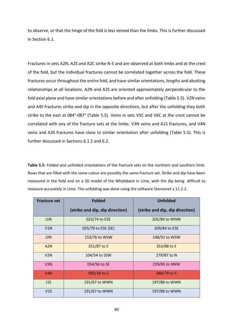
60

to observe, or that the hinge of the fold is less veined than the limbs. This is further discussed

in Section 6.1.

Fractures in sets A2N, A2S and A2C strike N-S and are observed at both limbs and at the crest

of the fold, but the individual fractures cannot be correlated together across the fold. These

fractures occur throughout the entire fold, and have similar orientations, lengths and abutting

relationships at all locations. A2N and A2S are oriented approximately perpendicular to the

fold axial plane and have similar orientations before and after unfolding (Table 5.5). V2N veins

and A4S fractures strike and dip in the opposite directions, but after the unfolding they both

strike to the east at 084°-087° (Table 5.5). Veins in sets V5C and V6C at the crest cannot be

correlated with any of the fracture sets at the limbs. V3N veins and A1S fractures, and V4N

veins and A3S fractures have close to similar orientation after unfolding (Table 5.5). This is

further discussed in Sections 6.1.2 and 6.2.

Table 5.5: Folded and unfolded orientations of the fracture sets on the northern and southern limb.

Rows that are filled with the same colour are possibly the same fracture set. Strike and dip have been

measured in the field and on a 3D model of the Whaleback in Lime, with the dip being difficult to

measure accurately in Lime. The unfolding was done using the software Stereonet v.11.2.2.

Fracture set Folded

(strike and dip, dip direction)

Unfolded

(strike and dip, dip direction)

J1N 023/74 to ESE 205/84 to WNW

V1N 025/70 to ESE (SE) 209/84 to ESE

J2N 153/76 to WSW 148/91 to WSW

A2N 351/87 to E 353/88 to E

V2N 104/54 to SSW 279/87 to N

V3N 054/56 to SE 239/85 to NNW

V4N 093/38 to S 088/79 to S

J1S 191/67 to WWN 197/88 to WWN

V1S 191/67 to WWN 197/88 to WWN

61

J2S 329/82 to ENE 326/86 to ENE

A1S 224/58 to NW 227/88 NW

A2S 176/68 to W 184/82 to W

A3S 254/72 to NNW 074/76 to SSE

A4S 270/54 to N 265/84 to N

5.4 Comparison of the fracture networks

5.4.1 Northern limb – qualitative description of fracture networks

The veins have a wide range of orientations and is dominated by abutting relationships in the

most eastern part of the limb. At Location 1, V3N and V4N veins appear to occur throughout

the lowermost part of the limb, with a wide range of orientations occurring (Fig. 5.16a). Veins

from set V3N become straighter and with a more limited range of orientations higher up on

the limb (Fig. 5.16b). The V3N veins become gradually less visible and/or decrease in

frequency westwards on the limb and are not observed at Locations 3 to 5 (Fig. 5.1). A more

systematic vein network with two set of orientations, V2N and V1N/J1N, is observed at

Locations 3 to 5 (Fig. 5.16c). As V3N veins become less visible westwards on the limb, V1N

veins become more closely-spaced and visible, creating a grid pattern with V2N veins (Fig.

5.16c). The V1N and V2N veins appear to cross-cut each other (Fig. 5.16c). Veins in sets V1N

and V2N may be more visible westwards because the lowermost part of the limb is located a

few metres longer down on the limb from the hinge of the fold, because the beach is a

downslope towards the sea and the fold plunges to the east.

62

Figure 5.16: Photographs from the northern limb, showing variations in the vein networks. a) Chaotic

network of veins, with a range of orientations, that are cross-cut by joints at Location 1. b) Vein

network with a more uniform orientation, upwards on the limb at Location 1. c) Systematic vein

network with mainly two set of veins cross-cutting each other perpendicular, observed further west

on the limb at Location 4. There is approximately 12.5m between photograph a)/b) and c) (Fig. 5.1),

with a gradual transition from randomly distributed to a more systematic vein network.

Joints in sets J1N and J2N are distributed along the entire northern limb and can be traced

across the fold (Fig. 5.15). Sets J1N and J2N appear to cross-cut each other obliquely, but with

a varying angle between them, where J1 curves towards the hinge of the fold in the eastern

part (Fig. 5.15). At Locations 1 and 2, J1N joints appear to curve towards the hinge, forming a

higher angle to the J2N joints and cross-cutting J2N at nearly 90° (Figs. 5.1, 5.5b, 5.15). Further

63

west, at Locations 3 to 5, these joints are straighter and appear to cross-cut each other at a

relatively lower angle (Figs. 5.1, 5.15).

In an underlying sandstone bed, outside the main focus area of the fold, a set of relatively

straight, parallel veins develop into an intense vein network that may be characterised as

breccia (Fig. 5.17). This sandstone bed is located closer to the core of the fold and further west

on the northern limb (Fig. 5.17). The bed is only exposed over an area of 22m2 and strikes 258°

at 36° towards the north. The veins in the intense vein network are filled with a white to yellow

mineral, with joints cutting through them. The intense vein network form irregular-shaped

pockets over an area less than 2m2 on the northern limb (Fig. 5.17). The intense vein network

is not located along faults and are not sedimentary breccias, but may be what Jébrak (1997)

describe as “hydrothermal breccias”. The relative age of this intense vein network is discussed

in Section 6.2.

64

Figure 5.17: a) Overview map of the Whaleback fold, with the red dot marking the location of the

intense vein network observation. b) Photograph taken at the red dot marked in a) at the northern

limb, showing how one set of parallel veins develop into closed brackets.

5.4.2 Southern limb - qualitative description of fracture networks

The southern limb generally shows more systematic fracture networks (e.g., at Location 6, Fig.

5.18a) than the fracture networks on the northern limb (e.g., at Location 1, Fig. 5.16), with a

65

more limited range of orientations and cross-cutting relationships (Fig. 5.18a). Grid patterns

are observed between the fracture of sets J2S and A1S, together with an oblique ladder

pattern between A1S and A4S, in the most eastern part of the southern limb (e.g., Location 6,

Fig. 5.18a). These fractures at Location 6 create grid patterns that are relatively smaller and

more closely spaced than the grid patterns further west on the limb at Location 7 (Fig. 5.18).

These systematic networks become less visible westwards on the limb, either because the

networks fade out or because they are more affected by weathering and erosion. The joints

that can be traced across the fold (J1S and J2S) together with A1S are easily observed on the

badly weathered surface at Location 7 (Fig. 5.18b). The rest of the observed fractures here

make up a network with a range of orientations that appear to be scattered around (Fig.

5.18b). The veins and joints observed in the lowermost part of the limb at Location 7 appear

to be similar to the pattern observed in the upper and most weathered part, but the surface

has a “polished” effect in the lowermost part (Fig. 5.18b).

66

Figure 5.18: Photographs of the southern limb, showing the variation of the fracture networks. a)

Photograph of Location 6, showing some examples of systematic fractures cross-cutting each other

and creating grid patterns. The yellow and blue circles show examples of these grid patterns. The

yellow circle marks the most closely spaced grid pattern, between J2S and A1S. The blue circle marks

the oblique grid pattern between A1S and A4S. b) Photograph of Location 7, further west on the limb

67

(Fig. 5.1), showing examples of two different grid patterns, between J1S/V1S and A1S and between J2S

and A1S. The grid pattern between J2S and A1S are relatively bigger than at Location 6. The lower part

of this photograph shows veins and joints with a wide range of orientations. Both photographs have

fractures of sets J1S, J2S and A1S marked on, to show that these sets are observed at both locations

despite the change in the other fractures.

The fracture network at Location 6 appears to be more systematic than at Location 7 (Fig.

5.19). In some parts of Location 7, it is hard to tell whether a feature is a fracture, or simply

something formed by erosion of the surface (Fig. 5.18b). In the uppermost part of Fig. 5.18b,

the surface is badly weathered and eroded, and it appears that the fractures are positive

topographic features, where the areas between the fractures are eroded (Fig. 5.18b). This may

be because the minerals along veins or adjacent to joints are more resistant to weathering

and erosion than the host rock. These observations are discussed in Section 6.1.

Figure 5.19: Length weighted rose diagrams (1 bin) of the fractures at the southern limb, a) Location 6

with 551 lines at an area of 1.3871m2, and b) Location 7 with 320 lines at an area of 1.03m2. Both rose

diagrams show a wide range of orientations, but Location 6 show a more systematic fracture network

with two set of fractures that tend to be the longest. Location 7 show a wide range of orientations with

relatively small differences in length compared to the fractures at Location 6.

68

5.4.3 Crest - qualitative description of fracture networks

The crest of the Whaleback fold is heavily eroded and weathered, with no clear variations in

fracture networks along the crest visible. Networks of 1-3 mm thick veins are observed in

areas, where the surface is more polished and not dominated by circular erosional features.

These networks of veins are not observed in the most heavily eroded and weathered areas at

the crest. In these heavily eroded and weathered areas, joints trending parallel to the fold axis

are the most prominent (set J4C). These fold axis parallel joints are distributed across and

along the crest of the fold. At Locations 9 and 10, some of the J2 joints (A6C at the crest) are

observed cutting across the entire fold close to vertical and as straight joints (Fig. 5.14). This

may indicate that these joints post-date folding. At Location 10, westwards at the crest (Fig.

5.1), A5C fractures are observed as either partly-filled veins or as joints around which

alteration has occurred. This can indicate that J1 are weathered-out veins on the limbs of the

fold, or that the veins observed at the crest reflect a secondary mineral filling of joints. Another

possibility is that A5C is a set of veins with a set of joints (J1) trending approximately parallel

to the veins. These observations are discussed in Sections 6.1 and 6.2.

5.4.4 Quantitative comparison between the networks in different parts of the fold

The comparison of the fracture networks in terms of geometry and topology is mainly focused

at Location 1 on the northern limb, Location 6 on the southern limb and Location 9 at the crest

(Fig. 5.1). There are fractures showing a wide range of orientations at each location, but when

the fractures are length weighted there are some orientations that stand out (Fig. 5.20).

69

Figure 5

.20: Length

weigh

ted ro

se diagram

s of all th

e fractures, in

clud

ing vein

s and

join

ts, and

plo

ts of len

gth ve

rsus o

rientatio

n at Lo

cation

1 at the n

orth

ern

limb

(a and

d), Lo

cation

6 at the so

uth

ern lim

b (b

and

e), an

d Lo

cation

9 at the crest (c an

d f). D

ata from

these grap

hs are b

ased o

n th

e same as th

e cum

ulative

plo

ts (Figs. 5.6, 5.7, 5.9, 5

.12 and

5.13).

5.12 and

5.13).

70

The fractures trending E/NE to W/SW tend to be the longest and most dominant at Location

1 (Fig. 5.20a). The longest and most dominant fractures at Location 6 show a narrower

orientation range, with two dominating sets trending ENE-WSW and WNW-ESE (Fig. 5.20b).

The fracture length is relatively similar for all orientations at Location 9, where a range of

orientations have relatively similar lengths, with no fracture orientations dominating (Fig.

5.20c). There are some spikes that are longer than the others at Location 9, but these are

widely scattered compared to the longest spikes that are more clustered at Locations 1 and 6.

The majority of the fractures at the three locations are shorter than 20 cm, with the longest

fractures located on the limbs (Fig. 5.20def). The fractures at the crest are shorter than 30cm

with the exception of a few fractures (Fig. 5.20f). This may be because the crest is more

weathered, resulting in fractures that appear to be segmented. Another possibility is that

Location 9 is smaller than Locations 1 and 6 and the fractures at the crest terminates outside

the interpretation area.

Table 5.6: Topological parameters at the northern and southern limb and the crest, retrieved from

NetworkGT.

Location 1 6 9

I-nodes 392 (18,03%) 246 (11,61%) 267 (32,56%)

X-nodes 461 (21,21%) 1159 (54,72%) 281 (34,27%)

Y-nodes 1321 (60,76%) 713 (33,66%) 272 (33,17%)

No. nodes 2174 (100%) 2118 (100%) 820 (100%)

No. branches 3100 3511 1104

No. lines 940 551 322

Area (m2) 1.4673 1.3875 0.5829

Nodes/m2 1482 1526 1407

Lines/m2 641 397 552

Average line length/ m2 0.0663 0.1381 0.2177

Connect/B (CB) 1.8735 1.9299 1.758

C-C 2653 3208 817

71

C-I 438 303 272

I-I 10 1 17

The northern limb (Location 1) is dominated by Y-nodes and the southern limb (Location 6) is

dominated by X-nodes (Table 5.6, Fig. 5.21). This means that the northern limb at Location 1

is dominated by abutting relationships and the southern limb at Location 6 is dominated by

cross-cutting relationships. The implications of these different node types for fluid flow are

discussed in Section 6.5.

72

Figure 5.21: a) Ternary plot showing the node dominance at the different locations, where the top

corner with “I” is 100% I-nodes, “Y”-corner is 100% Y-nodes and “X”-corner is 100% X-nodes. Location

1 show a dominance of Y nodes, Location 6 a dominance of X nodes and Location 9 a dominance of Y-

nodes. b) Photograph from Location 1 showing an example of the abutting veins on the northern limb.

940 lines have been digitised at Location 1, 551 lines have been digitised at Location 6 and 322 lines

have been digitised at Location 9.

Location 1, on the northern limb, has the highest number of lines per m2, with the veins being

the most closely-spaced (Table 5.6). The surface at the northern limb also has the highest

quality compared to the more weathered surface of the southern limb and the crest (Figs. 5.5,

5.8, 5.11). The number of abutting and crossing relationships is different at each limb, while

the crest shows an almost equal amount of abutting, crossing and isolated terminations. This

may be because the crest is the most weathered, and that one fracture might be weathered

where it appears to terminate as an isolated node. The cross-cutting relationships at the

southern limb are described as grid patterns in the qualitative description of the southern limb

(see Section 5.4.2). These abutting and cross-cutting differences are also reflected in the

connections per branch, CB (Table 5.6), with Location 6 having the highest value. This means

that the fracture networks at Location 6 are more connected than the fracture network at

Locations 1 and 9. The crest has the lowest CB and therefore a lower degree of connectivity

(Table 5.6), but there is higher uncertainty in the crest compared to the limbs because the

crest is more weathered. The consequences of interpreting and digitising a weathered surface

are discussed in Section 6.1.1.

5.5 Relative chronology and models for fractures in folds

The relative chronology of the fracture sets is mainly based on fracture types and abutting and

crossing relationships. It is common that a younger vein will abut or cross an older vein, while

a younger joint will typically abut an older joint (see Section 4.2.1). Based on the observations

on the Whaleback, there are two possible relative chronologies of the fracture sets on the

limbs. There are two possible chronologies because of the ambiguities related to the

determination of fracture types and origin, including whether the fracture sets denoted with

73

an “A” originated as veins or joints. In one scenario, J1 joints originated as V1 veins but have

been weathered- or eroded-out (Table 5.7).

Table 5.7: The relative chronology of the fracture sets. The columns in blue are a scenario where V1

and J1 are separated into different sets, with V1 veins older than the younger J1 joints. The columns

in yellow are the second scenario where V1 and J1 are the same set and originated as veins.

Northern limb Southern limb The crest

1 2 1 2 1 2

V2N

V1N

V3N

V4N

J1N

J2N

A2N

V2N

V1N/J1N

V3N

V4N

J2N

A2N

A4S

V1S

A1S

A3S

J1S

J2S

A2S

A4S

V1S/J1S

A1S

A3S

J2S

A2S

J3C

V5C

V6C

J4C

A5C

A6C

A2C

A5C

J3C

V5C

V6C

J4C

A6C

A2C

74

Figure 5.22: Schematic figures showing the chronology of the fractures on the Whaleback in scenario

1 from Table 5.7. Figures (a-d) show veins that pre-date folding, (e-f) show the fracture sets formed

during folding, and (g-h) show the fractures formed after folding. The fracture sets are labelled and

separated into different colours.

The first possibility is with the assumption that V1 and J1 are not the same set (Table 5.7). Sets

V1 and J1 have similar spacing and orientation but are observed on different parts of the limbs,

making correlation of these two sets difficult. There is therefore a possibility that these two

sets are not the same. On the northern limb, it is easy to distinguish between veins and joints,

with their abutting and crossing relationships making the relative chronology easier to

determine than on the southern limb and at the crest. The veins are interpreted to pre-date

folding and developed further during folding (Fig. 5.22). J3C joints corresponds with V3 veins,

75

and are determined to be weathered-out veins in the two scenarios, while A5C are interpreted

to have originated as joints in the first scenario (Table 5.7). J4C joints are formed during

folding, while the J1 and J2 joints are later, syn- or post-folding (Fig. 5.22). The relative

chronology on the southern limb and at the crest is mainly based on the abutting and cross-

cutting relationships of fractures, because the fracture type is difficult to determine.

Figure 5.23: Schematic figures showing the chronology of the fractures on the Whaleback in scenario

2 in Table 5.7. Figures (a-d) show veins that pre-date folding, (e-f) show the fracture sets formed during

folding, and (g-h) show the fractures formed after folding. The fracture sets are labelled and separated

into different colours.

76

In the second scenario, sets V1 and J1 are assumed to be the same set, where joints of sets J1

are weathered-out veins, reflecting areas that are more weathered and/or eroded (Table 5.7,

Fig. 5.23). A5C fractures are observed as partly-filled veins at Location 10 at the crest, and

therefore interpreted to have originated as veins in this scenario (Table 5.7). A5C corresponds

to the sets V1 and J1, where A5C have had more minerals removed compared to the V1 veins

(Fig. 5.23). The relative chronology at the crest is difficult to determine because of weathering,

making the determination of the relative ages of the different fractures reliant upon the

fracture sets on the limbs. For example, set A2C is interpreted to correspond with sets A2N

and A2S, which abut joints on the limbs, indicating they are the youngest fractures. These

possible, relative chronologies and the significance of this is discussed in Section 6.2.

77

6 Discussion

This chapter discusses the following:

1. The validity of the data and methods used in this thesis.

2. A model of the deformation history, variations in fracture patterns across the fold and

the significance of this.

3. Implications for models of fractures in folds, with implications for reservoir models.

4. Implications of the results for using exposed examples to develop fracture models for

subsurface reservoirs.

6.1 Data and methods

This section discusses problems involved with the data and methods, including: (1) problems

related to the weathering and erosion, (2) dividing fractures into sets, (3) distinguishing

between fracture types, (4) examples of possible errors in fracture interpretation caused by

weathering of the Whaleback, and (5) problems digitising and using the software.

6.1.1 Errors related to interpreting a weathered surface

Interpretations of fractures can be affected by weathering of the rock surface. Weathering of

the Whaleback fold can affect the interpretation of fracture type, terminations, fracture

relationships, length, etc. The quality of the exposure varies on the Whaleback fold depending

on altitude and exposure to wave action. The field area is situated in the tidal zone, and the

tidal range in the area is up to ~7.5m. The northern limb has a more “polished” surface than

the southern limb and the crest, because it is most exposed to wave action and mechanical

erosion. The crest and the uppermost part of the southern limb show circular erosional

features, where the crest is most weathered, perhaps because it is higher up, so it is less prone

to mechanical erosion than the limbs. The smooth and polished surfaces on the northern limb

show a network of veins and joints that can easily be distinguished from each other. The more

weathered surfaces on the southern limb show fracture networks where it is uncertain

whether a fracture is a vein or a joint, and the correlation of fractures is difficult. This can

create ambiguities in interpretation of fracture relationships and therefore affect the

78

determination of the relative ages. The differences in qualities of the exposed surfaces might

make the comparison of the different surfaces invalid, with the qualities of the surfaces

affecting the level of details in the way that one fracture set might falsely be separated into

two different sets or vice versa.

The Whaleback fold has been observed in the field and analysed using a 3D model of the fold,

but to get an understanding of how the level of details can affect the interpretation of

fractures the Whaleback fold has been analysed using drone images taken from three

different altitudes: 120m, 50m and 10m (Fig. 4.2). The level of details increases with

decreasing altitude or distance from the interpretation area. This experiment shows how the

dominance of the different fractures vary and how the different fractures become more

significant at specific altitudes. At an altitude of 120m, the only visible fractures are the ones

that can be traced across the fold, J1 and J2 (Fig. 4.2). At this altitude, it is relatively easy to

identify the longest fractures without the interruption of shorter and more chaotic fracture

networks. This is, however, not detailed enough to interpret the relationships between the

fractures. This is also the case for the drone images taken at an altitude of 50m, but at this

altitude more details of the fracture networks and the surfaces are visible (Fig. 4.2). When it

comes to understanding abutting and cross-cutting relationships, the level of details is not

enough at 50m altitude (Fig. 4.2). Nevertheless, images taken at this altitude are useful for

observing changes in frequency among the longest fractures. For example, the NNW-SSE

trending joints (J2) at the northern limb becomes more visible westwards on the fold. At 10m

altitude, the thickest veins on the lowermost part of the northern limb can be observed. The

thinner veins are, however, difficult to observe and even harder to trace. The joints traced

across the fold are not as dominant as on the images taken from an altitude of 50m, and the

weathered surface with its erosional features becomes more visible as the level of details

increase. The effect of weathering and erosion becomes one of the dominant features, making

the fracture network interpretation difficult. It is hard to distinguish between the fractures

and the erosional features at the crest on the images taken from an altitude of 10m. None of

these altitudes show a high level of detail for the veins. Most of the veins would not be

included if the interpretations and analyses were made using photographs taken at any one

of these altitudes.

79

Subjective bias relates to how individuals perceive, collects and interprets geological data

(Bond et al., 2015). The observations and digitising of fractures I have made on the Whaleback

are subjective, and other geologist may end up with different results when, for example, they

divide fractures into sets. Andrews et al. (2019) quantified subjective bias in fracture data

collection to investigate the scale, nature and consequences of subjective bias, showing that

subjective bias affect fracture statistics and that it mostly affects the small scale fracture

features. This may perhaps not be that relevant as long as there is consistency in the analysis

and interpretations. Errors can occur if, for example, fracture networks are interpreted

differently from one location to another. Fracture observations on the weathered surfaces of

the southern limb and the crest increases subjectiveness in the characterisation of veins and

joints. In some areas on the southern limb there are traces of purple alteration that are shaped

as fracture traces. If these alteration traces are in fact weathered-out veins or joints, then they

should be included in the analyses. These traces are, however, not possible to determine as

traces of fractures for certain and have not been included in this thesis. This example show

how undersampling of fractures may occur and are related to interpretations made on

weathered surfaces.

6.1.2 Dividing fractures into types and sets

Geologists may produce different results when dividing the fractures into sets, as this process

is individual and creates subjective biases. There are not clear standards for dividing fractures

into sets and the methodology can differ from geologist to geologist. Dividing fractures into

sets is, however, beneficial in understanding the relative ages of the different structures if age

is included in one of the criteria for defining sets. In this thesis, fractures are classified and

termed veins, joints or fractures, and divided further into sets based on orientation, fracture

relationships, etc. The fractures not meeting the criteria of a vein or joint were termed

“fracture”, with a label “A” (Section 4.2). This generalisation of veins and joints complicates

the determination of the relative ages, because the relative ages are based upon fracture type

and their abutting and crossing relationships (Section 4.2.1). As seen in the cumulative graphs

(Figs. 5.6, -7, -9, -12 and -13), the fractures display a wide range of orientations that makes

80

the process of dividing them into sets difficult and with more ambiguous sets than identified

in the Price model. The significance of the implications related to dividing fractures into sets

is that the ambiguities make comparisons of fracture sets in the different locations difficult.

This has implications, for example, in testing the Price model. For example, veins in set V3N

on the northern limb of the fold has been identified as developing from striking NE to ENE,

which is a relatively wide range of orientations. These veins can appear to be two sets of veins

when only studying fracture orientations in a rose diagram (Fig. 5.10a) but are interpreted as

being one set of veins formed at the same time in the field, because they can be correlated

together from striking NE to ENE higher up on the exposed limb. The weathered surfaces at

the southern limb and the crest made the determination of fracture types and their

relationships difficult, with ambiguity related to the origin of these brown-filled fractures at

the southern limb. This is further discussed in Section 6.2.

6.1.3 Examples of possible errors in fracture interpretations caused by weathering

Weathering and erosion make it difficult to define fracture types, age relationships and

kinematics. Fig. 5.18 shows fractures that mutually cross-cuts each other on the southern

limb, creating a grid pattern that would be “shear joints” in the model of Price (1966). There

are, however, no shear displacements observed along these fractures on the Whaleback. The

fracture type origin of these mutually cross-cutting fractures is unclear, which makes the

relative ages difficult to determine as it cannot be based on abutting relationships or fracture

type. Erosion of the bedding planes can influence the determination of fracture types and

their relationships. Some areas on the southern limb show an undulating topography, where

fractures in some cases are observed as veins in the higher elevated parts of the undulated

surface and continues as a joint in the lower elevated parts (Fig. 6.1). The fractures can in

some cases be correlated at each side of the lump, while others appear to terminate

somewhere on the lumps and cannot be correlated further (Fig. 6.1).

81

Figure 6.1: Photograph of Location 6 on the southern limb, showing the undulating topography of the

exposed surface. The circles in red and green marks examples of higher elevated parts (lumps) of the

surface, with the dashed lines in blue and orange showing examples of fractures observed within these

areas. The dashed blue line is observed as a white mineral-filled vein within the green circle and as a

brown-filled fracture outside the circle. The orange dashed lines show examples where fractures are

segmented and appear to terminate towards the higher elevated parts of the surface.

The joints that strike parallel to the fold axis (J4C) at the crest appears to be segmented, where

it is difficult to separate the segments because of the circular erosional features on the

exposure (Fig. 5.11). A5C have been correlated with J1N and J1S, but it is unclear whether they

are veins or joints (Section 5.2.3). A5C are observed as joints further east at the crest at

Location 9, where the fold plunges to the east, with Location 9 having a more weathered

surface than at Location 10 further west (Fig. 5.1). At Location 10, A5C are observed as partly-

filled veins, meaning that A5C may be weathered-out veins or joints around which alteration

has occurred. The veins observed at the limbs cannot be traced in the field up towards the

uppermost part of both limbs, where the joints are observed. There can be three possibilities

if the joints at Location 9 are the same set as the partly-filled veins at Location 10. First, the

mineralising fluid did not completely fill the fractures. This can be a result of a reduction in the

82

fluid flow that resulted in not enough minerals reaching the fracture. Second, a later fluid may

have dissolved some of the minerals in the subsurface. Third, weathering at the surface may

have removed some of the minerals, and this may be the case on the southern limb. An

example of this is the brown-filled fractures (Fig. 5.8), which might be weathered-out veins or

alteration around joints. The fact that these brown-filled fractures are only observed locally

on the southern limb, can indicate that the alteration is a near-surface process. There are two

possible explanations for observing veins in the lower part of the limbs that cannot be traced

upwards, closer to the crest:

1. The hinge region is less veined than the limbs, which is contrary to models of folding

in sequences like this (Ramsay, 1967, 1974).

2. The veins are more weathered and harder to observe in the crest, which has

significance for the sampling, e.g., falsely interpreted to be joints or undersampling.

The J2 joints can be traced across the fold, with what appears to be a subset of shorter joints

observed on the southern limb. The joints in the subset are partly to fully filled with the same

brown fill as the other fractures on the southern limb, but where these fractures appear to

abut A1S there is, in some cases, a thin white (1mm) trace with purple alteration around it,

continuing for a few centimetres after the apparent abutment. The lengths and terminations

of these subset-fractures are therefore hard to determine and might be longer and different

than observed. The fracture type origin of J2 is also difficult to determine, as they are observed

as joints along the limbs, as both joints and in some cases, partly-filled veins at the crest and

with a subset of partly-filled veins on the lowermost part of the southern limb. This may

indicate that the J2 joints originated as veins, where the joints in this set are weathered-out

veins. The number of lines per m2 at Location 9 at the crest is higher than at Location 6 on the

southern limb (Table 5.6), which is compatible with the statement of Cosgrove (2015) that the

hinge region in folds is the site of the most intense fracturing. There are, however, 641 lines/

m2 at Location 1 on the northern limb compared to 552 lines/m2 at Location 9 at the crest

(Table 5.6). One possibility for this number being higher on the northern limb compared to

the crest, might be because weathering makes it harder to see fractures at the crest.

83

6.1.4 Problems digitising the fracture networks

The results of digitising in QGis are influenced by the angle between the line of view and the

surface being digitised, and the quality of the photograph. The photographs that are imported

into QGis and digitised need to be taken or corrected to be perpendicular to the surface

because this can influence fracture lengths and orientations. The interpretation of fracture

lengths can be hard to determine with certainty in the case of the Whaleback because of

weathering. Deciding the fracture length is also affected by the erosion and topography of the

exposed surface. Undulating topography can cause straight veins and joints to appear to be

curved can and divide fractures into apparent segments, where the fractures cannot be

observed in the higher elevated parts of the surface (Fig. 6.1). The lengths of the fractures

from digitising are only measured within specific locations, meaning that fractures that extend

beyond the location and interpretation area will be measured as shorter than they actually

are.

Distinguishing between veins and joints is problematic when the veins and joints are merged

to one linestring in NetworkGT (Section 4.1.1). It is possible to add a filter to only run the

analyses on one or several features (e.g., only the joints) by adding a filter using the Query

Builder. This can be useful when comparing the orientations of veins, joints and fractures.

NetworkGT is designed, however, to only run analyses on one linestring at the time, meaning

that the relationships between the fractures is included, but the information about what

fracture type abuts another is not (e.g., if a joint abuts a vein). For example, the joints that

actually abut a vein will be classified with isolated terminations when filtered to only run

analyses on the joints. This is because the veins are excluded in the filter, so instead of creating

abutting, Y-nodes, the software classify the terminations as isolated, I-nodes. This means that

the results of the analyses need traditional geological interpretation to separate the fracture

types when determining the relative ages of the fractures. The filter was only used in this case

to compare the orientations and lengths of the veins, joints and undefined fractures when

identifying fracture sets. In the case of the Whaleback, the fractures show a combination of

different structures, where the merging of which may not be geologically meaningful.

84

Before adding the filter, I compared the following two methods: (1) separating the veins, joints

and/or fractures in separated linestrings, and (2) by merging the different fracture types to

one linestring. I compared the topological parameters for both methods at Locations 1, 6 and

9. In all three cases, by separating the fractures types in separated linestrings, the number of

nodes and branches decreased and there was an increase in number of I-nodes and I-I

branches compared to the merged linestring. As the number of branches decreased in the

separated linestring files, there were increases in both connection per branch and branch

length. This comparison shows how strongly the relationships between the different fracture

types affects topological analyses and how not taking the relative ages and fracture types into

account can be misleading and affect further geological analysis and interpretations. The

fractures on the Whaleback fold show a wide range of orientations and crossing and abutting

relationships, where more than two fractures appear to mutually cross-cut or abut each other

at the same point (Fig. 6.2). This creates a problem in NetworkGT as the toolbox detects

multiple intersections in one point.

Figure 6.2: Photograph from Location 1 on the northern limb, showing an example of a situation where

three fractures abut or cross-cuts at the same point, marked with a white circle. The dashed red, green

85

and blue lines are veins (A and B) and a joint (C), where the green and red line cross-cuts and the blue

line abuts at that very same point.

Fig. 6.2 shows that vein B abuts the older vein A, with the joint C being the youngest and cross-

cutting both. The relationship between A and B is first abutting, creating a Y-node, with C

crossing to create an X-node. The scenario where an intersection is classified as both an X- and

Y-node is not included in NetworkGT. To avoid creating this error, the abutting fracture (blue

dashed line in Fig. 6.2) is “snapped” to abut only the red or the green dashed line.

6.2 Model for the history of deformation

6.2.1 Evidence of pre- and syn-folding fractures

The en echelon veins of set V2 show fibres that trend NE-SW, indicating an oblique opening.

These veins are determined to be the oldest fractures based on abutting and crossing

relationships. Some of the en echelon veins can appear to abut V1 (Fig. 6.4c), but this may be

because some V1 veins cut V2 veins at the termination of one vein array tip. Based on the

orientation after unfolding (Table 5.5), sets V2N and A4S are assumed to be the same set,

formed pre-folding (Table 5.4, termed V2). V3N veins have the same orientation as A1S

fractures when unfolded (Table 5.5), and are interpreted to be the same set, initiated after V2

veins and pre-folding (Table 5.4, termed V3). This is also the case for sets V4N and A3S (Table

5.4, termed V4), which initiated after set V3, based on the abutting relationships. Set J3C at

the crest may be the same set as V3 based on the similar orientation, spacing and the abutting

relationships to set V1 (Tables 5.1, 5.2, 5.3), where J3C joints are weathered-out veins at the

crest. There is, however, ambiguity related to the correlation of the fractures sets at the crest

because of weathering and because many fracture sets can only be observed at the polished

areas at the crest. Sets A4S, A1S and A3S are termed “fractures” on the southern limb but are

interpreted to have originated as veins, because they are interpreted to correspond with the

vein sets V2N, V3N and V4N (Section 5.3).

86

Sets V1 and J1 show similarities in orientation, spacing and abutting and crossing relationships

(Tables 5.1, 5.2, 5.3), but are different fracture types. At Location 4 on the northern limb (Fig.

5.1), set J1N occurs on the lowermost part of the exposed limb, parallel to set V1 (Fig. 6.3).

The areas where set J1 is observed appear to be more fractured than the surroundings, and

those areas are dominated by joints (Fig. 6.3), whereas the areas where V1 are observed are

dominated by veins. The V2 veins that joints of set J1 cross-cut, are partly-filled with minerals

and weathered in these more fractured areas (Fig. 6.3). This may indicate that sets V1 and J1

are the same set and that, on the lowermost parts of the limb, joints of set J1 are actually

weathered-out veins. Set J1, however, consists of joints on the upper parts of both limbs and

then as joints and partly-filled veins at the crest (A5C). One possibility is that sets V1 and J1

are not the same set of fractures, with J1 following the pre-existing veins of V1 during

formation. Another possibility is that V1 and J1 are the same fracture sets initiated as veins

pre-folding, where some veins have had all the minerals removed and some that have only

some of the minerals removed. Set V1 formed after set V2, and before sets V3 and V4, because

sets V3 and V4 abut V1 veins.

87

Figure 6.3: Photograph of Location 4 on the northern limb (Fig. 5.1) showing sets V2 and V1 mutually

cross-cutting each other and set J1 on the lower part of the limb. There appears to be narrow zones of

weathering (green dashed rectangle) where there are few veins observed within the areas of the joints.

The green dashed circle shows examples of areas that are dominated by veins.

The intense vein network observed in an underlying sandstone bed of the main focus bed (Fig.

5.17) can be evidence of syn-folding fractures because they are only observed close to the

hinge. Fluids may migrate from the inner to outer arc of folds formed in homogenous

anisotropic layers (Cosgrove, 2015), and the intense vein network is only observed in the

underlying sandstone bed. Set V5C is only observed on the polished areas at the crest and V6C

is scattered across the crest (Fig. 5.11) and do not correspond to any of the fractures at the

limbs based on the orientations and results after unfolding. Set V5C and V6C probably formed

88

during folding because they are cut by J4C joints at the crest (Table 5.3), and only occur at the

crest. The joints striking parallel to the fold hinge line (J4C) at the crest may also have formed

during folding, but after the mineralisation phase that formed V5C and V6C (Figs. 5.22-23).

The joints in J4C may represents outer-arc extension fractures trending parallel to the fold

axis, as described by Cosgrove and Ameen (2000), Li et al. (2018) and Wu et al. (2019) (Section

2.4.2). Several studies describe pre- and syn-folding veins in North Cornwall, (e.g., Mackintosh,

1967; Beach, 1977; Jackson, 1991), with it being possible to link some of the veins in those

studies with the vein sets described in this thesis (Fig. 6.4). The vein sets marked “V1” and “B”

in Fig. 6.4(a) and C1 in Fig. 6.4(b) corresponds with set V2 in this thesis, with “B” and “E2”

representing the en echelon veins observed on the northern limb. Set C2 in Fig. 6.4(b) is

termed set V1 in this thesis (Fig. 6.4c).

Figure 6.4: a) Schematic figure of veins in normal fold-limbs at Millook Haven, shown by Jackson (1991,

figure 3a). Notation used by Jackson (1991): V1 – regional distributed veins, A – en echelon veins, B –

89

en echelon veins, S – forked and branching terminations. A and B are described as conjugate sets of en

echelon veins, initiated from the principal veins V1 (V2N in this thesis). Set A is not observed on the

Whaleback fold and not discussed further. b) Schematic figure of veins in normal fold-limbs at Millook

Haven, from Beach (1977, figure 6). Notation used by Beach (1977): C1 and C2 - principal veins, E1 and

E2 - en echelon zones, T – tensile veins and B – branch fractures. c) Photograph from Location 1 at the

northern limb, showing en echelon veins within the red rectangle termed B in a) and E2 in b). V1 and

V2 in this figure are the vein sets described in this thesis, where V1 correlates to C2 in b) and V2 to V1

in a) and C1 in b).

Jackson (1991) show veins that trend NW-SE and that have been formed prior to, and during

folding, which correlated with the en echelon veins of set V2 in this thesis. The en echelon

veins observed on the northern limb of the Whaleback appear to indicate E-W dextral

transpression, which is compatible with the interpretations of Jackson (1991).

6.2.2 Evidence of post-folding fractures

J2 joints are observed along and across the Whaleback fold, as relatively straight joints cutting

all veins (Fig. 5.14). These joints, together with fractures of set A2, formed after the veins and

joints in set J4C (Figs. 5.22-23). Set J1 pre-dates set A2 based on abutments in both possible

scenarios (Table 5.7), regardless of whether set J1 are weathered-out V1 veins or originated

as joints. The relative ages of sets J1 and J2 are difficult to determine if J1 and V1 are not the

same set, because J1 and J2 appear to mutually cross-cut each other. Sets A2N, A2S and A2C

(termed A2) trend N-S and are determined as being the youngest based on its abutting

relationships (Figs. 5.22-23). A2 fractures are observed as veins, partly-filled veins and as joints

across the fold, where set A2 are only observed as joints at one location (e.g., Location 1) and

as both joints and partly-filled veins further west on the limb (e.g., Location 4). This may

indicate that A2 is two set of fractures, with the joints following pre-existing veins, or that set

A2 originated as veins where some veins are more weathered and have had more minerals

removed. Sets V2, V1, V3 and V4 on the southern limb are filled with a brown material

compared to the white mineral fill in some of the A2 fractures, suggesting that the veins (V2,

V1, V3 and V4) may have been weathered before the mineralisation of set A2. The white-filled

A2 set on the southern limb cross-cuts the other fractures, which indicates A2 originated as

90

veins. This also means that if set A2 originated as veins, that the fractures cut by A2 have also

originated as veins, because it is uncommon to see veins abutting joints.

6.2.3 Sequence of events

Syn-sedimentary, syn- and post-lithification and pre- and post-folding events have occurred

within the rocks of the Whaleback fold. The Bude Formation was deposited in the Late

Carboniferous and this may include syn-sedimentary faulting seen in Fig. 6.5 (Whalley et al.,

1986; Higgs, 1991). The Formation experienced a deformational phase early after deposition

with the onset of the Variscan deformation. The vein sets (V2, V1, V3, V4) initiated during this

deformational phase, prior to folding of the sediments and continued to evolve during folding

(Figs. 5.22-23). The orientation and fibre in the en echelon veins show that the maximum

principal stress was NW-SE prior to and during folding, with Jackson (1991) showing that the

obliquity to the approximately E-W trending folds is consistent with E-W dextral transpression.

This was followed by a deformational phase of flexural slip folding including the development

of the Whaleback fold, formation of vein sets V5C and V6C, followed by the joints trending

parallel to the fold axis, set J4C. Mineralisation ceased after the formation of the vein sets V5C

and V6C at the crest and before the formation of the J4C joints. The intense vein network

observed in an underlying sandstone bed was formed during this folding event, before joint

set J4C. Lloyd and Whalley (1986) reports that there is south-directed shear in the region post-

folding, but there is no clear evidence for this on the Whaleback, although it is possible the

faults shown in Fig. 6.5 are related to this event. Post-folding fracturing includes sets J2 and

A2. These may have formed during Mesozoic basin development, Cenozoic ("Alpine")

contraction, or during exhumation.

91

Figure 6.5: Photograph of fault traces in shale and silt beds on the northern limb, which underlie the

bed that is the main focus of this thesis. This location is within a metre of the fold hinge. The apparent

movement senses in their current configuration are labelled with arrows, with some faults extending

bedding and others indicating contraction. The faults are located within a folded bed that dips 40° to

the north.

6.3 Variations in fracture patterns

The fracture networks on the Whaleback fold show spatial variations along the limbs and

across the fold (Section 5.4). The fracture patterns vary in terms of abutting and crossing

relationships (Tables 5.1, 5.2 and 5.3), distributions along the limbs (Tables 5.1, 5.2 and 5.3),

orientations and lengths (Fig. 5.20), and topological parameters (Table 5.6). The change from

a vein network with a range of orientations, to a network of relatively straight parallel veins

cross-cutting each other close to perpendicular located on the northern limb, show how

fracture patterns can vary on a metre scale within the same bed. The intense vein network

observed in an underlying sandstone bed shows how fracture patterns can vary between

different beds (Fig. 5.17). These variations show that the fracture networks on the Whaleback

fold are heterogenous and can affect the testing of models for fractures in folds. This is further

discussed in Section 6.5.

92

It is unclear whether the brown-filled material along or around the fractures on the southern

limb are the result of weathering along veins or alteration around joints. Joints usually abut

earlier joints, while veins can cross-cut or abut earlier veins. This means that distinguishing

between veins and joints is beneficial in understanding the relative ages, because veins are

generally older than the joints within the same rock. Whether a fracture network consist of

veins or joints is important in terms of permeability and fluid flow, as veins can be completely

filled with minerals, in which case they may act as barriers to fluid flow. The northern and

southern limb differ in node dominance (Table 5.6), with abutting relationships dominating

on the northern limb (Y-node) and crossing relationships on the southern limb (X-node). This

may influence permeability, but have to be tested and is not further discussed in this thesis.

The heterogeneities in the fracture networks on each limb is also reflected in the length versus

orientation plots (Fig. 5.20), where the majority of the fractures at Location 6 on the southern

limb tend to be longer than at Location 1 on the northern limb.

6.4 Implications for models of fractures in folds

Price (1966) proposes up to four joints sets on each limb occur in anticlines; a pair of conjugate

shear joints (S1 and S2, S3 and S4), one set of joints striking parallel (T1 and T2) and one set of

joints striking perpendicular (T3 and T4) to the fold hinge line (Fig. 6.6).

93

Figure 6.6: Block diagram showing the four predicted joints sets in an anticline, from Price (1966). S1,

S2, S3 and S4 – pairs of conjugate shear joints, T1 and T2 – joints that strike parallel to the fold hinge line,

and T3 and T4 – joints that strike perpendicular to the fold hinge line.

The orientations of the J1 and J2 joints (Figs. 5.1, 5.14 and 5.15) on the Whaleback may relate

to the conjugate shear joints on the fold limbs in the Price model based on orientations and

that the joints appear to mutually cross-cut each other (S1 and S2, S3 and S4 in Fig. 6.6). There

are, however, no shear displacements observed along these joints on either limb on the fold.

The joints of J1 and J2 intersects the fold hinge line asymmetrical and at different angles from

the Price model, where the “shear joints” in the Price model are conjugate about a line

perpendicular to the hinge. The sets J1 and J2 are not conjugate about a line perpendicular to

the hinge, but J2 joints intersect the fold hinge line close to perpendicular (Figs. 5.14, 6.6). The

J1 joints furthest east on the Whaleback fold appear to be curved and intersecting the fold

hinge line at a relatively lower angle than further west on the fold, which do not correlate to

the joints in the Price model. Pollard and Aydin (1988) address the validity of shear joints, and

suggest that a fracture with a shear displacement should be called a fault rather than a shear

joint.

The Whaleback fold have veins that resemble the T1, T2, T3 and T4 joints in orientation in Fig.

6.6, trending close to parallel and perpendicular to the fold hinge line on both limbs. The age

relationships between the T-joints and S-joints are not discussed in the Price (1966) model,

but the relative ages of the fractures trending parallel and perpendicular on the Whaleback

(A2 and V4) are different. Fracture set A2 are oriented close to perpendicular, and vein set V4

are oriented close to parallel to the fold hinge line respectively. Fracture set A2 is similar to T3

and T4, and vein set V4 to T1 and T2 in Fig. 6.6. A2 fractures are interpreted as being the

youngest of all fractures on the Whaleback, formed post-folding because they abut sets J1 and

J2, and cross-cut all veins. V4 veins trend close to parallel to the fold hinge line and have been

interpreted as pre- and syn-folding, formed after V3 based on abutting relationships. The V4

veins was formed before the mineralisation ceased and the J4C joints at the crest was formed.

94

The only apparent characteristic the V4 veins and A2 fractures on the Whaleback fold share

with the T-joints in the Price model, is orientation.

The Price (1966) model is for joints in folds, but many of the fractures on the Whaleback fold

are veins. Whereas a joint will typically abut an older joint, veins commonly cross-cut earlier

veins (see Section 4.2.1), so veins and joints can show different patterns. The fracture pattern

displayed in the Price model (Fig. 6.6) do not correspond to the fracture pattern on the

Whaleback fold, with differences in fracture types, intersecting angles to fold hinge line and

the fracture relationships. The fracture pattern can be difficult to predict if there are pre-

existing fractures that pre-date folding. The Price model appears to assume that the joints and

the fold are the same age, which is not the case for the Whaleback fold. Some of the veins on

the Whaleback fold pre-date folding and can influence further fracturing during folding. The

joints on the Whaleback fold are interpreted to post-date folding, except for J4C that are

interpreted to have formed during folding. This means that the post-folding joints on the

Whaleback do not need to show the patterns in the Price model, which suggests that it is

unsafe to use the Price model for joint distributions in folds. Watkins et al. (2018) compare a

field study of fractures in a thrust belt to the Price (1966) model and concluded with that on

a large-scale, 3D model of several folds, their data match the Price (1966) model. On a smaller

scale, within the individual fold structures, the fracture attributes vary more and become

more difficult to predict (Watkins et al., 2018). This may also be the case for the Whaleback

fold, where different fractures dominate or stand out more in drone images taken at different

altitudes (Fig. 4.2).

6.5 Implications for reservoir models

Models of fractures in folds are especially important for the petroleum industry because folds

can be potential hydrocarbon reservoirs, where understanding fracturing can be used to help

understand hydrocarbon migration and reservoir quality (Casini et al., 2011). To properly

understand the fracture system, it is important to distinguish between fractures of different

mechanical origin (i.e. joints, faults etc.), the relative chronology of the fractures and their

relationships to the tectonic episodes of the area (Casini et al., 2011). Developing models from

95

exposed analogues can be difficult as quality of the exposures and related structures can vary

both on a large, and especially, on a small scale (Al-Kindi, 2020). There are a wide range of

factors, including lithological and structural, that influence fracture formation, and these can

cause the resulting fracture networks to be heterogeneous and difficult to predict (Watkins et

al., 2018).

There are many cases on the Whaleback fold in which it is unclear whether a fracture is a

weathered-out vein or a joint around which alteration and/or weathering have occurred. In

some cases, what appears to be a partly-filled vein is actually a joint in which sand has

accumulated. Joints are open-spaced fractures and when well-connected they can provide

continuous pathways for fluid flow (Odling et al., 1999). Veins that are completely filled with

minerals do not currently transmit fluids and have a lower permeability than joints (McGinnis

et al., 2015). This means that if all the fractures on the Whaleback were predicted to be joints,

the Whaleback would display open pathways for fluids and lead to incorrect results, because

most fractures on the Whaleback originated as veins. This shows that the use of exposed

analogues in reservoir modelling can give incorrect results for fluid flow. Two possible relative

chronologies are suggested in the Whaleback’s case, because of uncertainties related to

fracture type and origin. Sets J1 and V1 are interpreted to be the same set, where set J1 is

weathered-out veins. Predicting the permeability and fluid flow conditions can be difficult in

this case, because the veins in sets J1 and V1 are weathered differently. The weathering

appears to be a near-surface process, because of local variabilities on the Whaleback fold. Sets

J1 and V1 can be completely filled veins in the depth, where the weathered surface of the

Whaleback fold may differ from the subsurface.

The fracture pattern and densities can be predicted by assuming that the strains

accommodated by fractures mimic the bulk strains within bedding during folding (Lisle, 1994,

2000). Others predict joint orientations based on the curvature, by assuming joints trend

parallel to the minimum curvature of an elastically deformed layer (Ericsson et al., 1998;

Fischer and Wilkerson, 2000). Such models that use strain or curvature as proxies for joint

distributions are commonly used in the petroleum industry (Lisle, 1994; Ericsson et al., 1998;

96

Fischer and Wilkerson, 2000; Hennings et al., 2000). The distributions and frequencies of the

different fracture sets vary along the limbs and at the crest in some cases, where, for example,

J2N increases in frequency and/or visibility westwards on the northern limb. This appears,

however, to be a result of local weathering and/or erosion of the J2 joints. The crest on the

Whaleback fold have a higher number of lines per m2 than on the southern limb (Table 5.6),

which is common on curved surfaces because the hinge region is the area of high strain in

folds (Pearce et al., 2011; Cosgrove, 2015). The number of lines per m2 is, however, higher on

the northern limb on the Whaleback fold, with Pearce et al. (2011) showing that there is no

significant correlation between surface curvature and fracture density on the Whaleback.

Joint formation on the Whaleback fold might be a near-surface process like weathering and

erosion, and that data for joint distributions at the surface may not reflect what is happening

in the subsurface. Joints in exposed rocks may have developed during exhumation, increasing

the fracture density compared to exposures at reservoir conditions (Sanders et al., 2003). The

varying fracture distributions, influenced by weathering and erosion, across the Whaleback

fold make it hard to use this exposure to prove models for subsurface reservoirs. The Price

model is specifically for joints within folds, where if exhumation and joint formation occurred

years after folding, there is no reason for the Price model or models that relate strain or

curvature to the distribution of joints, to apply.

97

7 Conclusions

The Whaleback fold at Bude, SW England, is a well-exposed metre-scale anticlinal pericline

that provides an opportunity to test models for the distributions of veins and joints in a fold.

The limbs and crest of the Whaleback fold show exposures with varying degrees of weathering

and erosion that affect the interpretation of the fracture network. The Whaleback fold shows

veins and joints, as well as other fractures that may be either veins or joints. Seven sets of

fractures have been identified at each limb and at the crest, with three sets at the crest that

do not correspond to the fracture sets at the limbs. A total of ten distinct sets have therefore

been identified across the Whaleback fold. Four sets of veins are interpreted to pre-date

folding and developed further during folding, based on the orientation when unfolded and on

fibre orientations. Two sets of veins and a set of joints at the crest are interpreted to have

formed synchronously with folding, because of the positions on the fold. Some joints are

traced across the fold as relatively straight and vertical joints, and are interpreted to post-date

folding.

The joints on the Whaleback fold do not show evidence to support the patterns of joints

predicted by Price (1966), because the majority of the joints on the Whaleback are interpreted

to post-date folding. The post-folding joints on the Whaleback, intersects the fold hinge line

at different angles and have different orientations than the joints in the Price (1966) model.

This is probably because the Price model makes the assumption that the joints formed during

folding, which is not the case for the joints on the Whaleback fold, except for one set of joints

at the crest that have been interpreted to be formed during folding. This suggests that the

Price (1966) model should not be used to predict joint patterns, if there is evidence that the

joints did not form during folding. Similarly, the number of lines per m2 show that fracture

frequencies are not significantly lower on the limbs compared with the crest. This supports

the interpretation of Pearce et al. (2011), who show that there is no significant correlation

between curvature and fracture density on the Whaleback fold. Although models that use

strain or curvature in folds to predict the distribution of open fractures (joints) in the

subsurface (e.g., Lisle, 1994; Ericsson et al., 1998; Fischer and Wilkerson, 2000; Hennings et

98

al., 2000), and to thereby predict reservoir quality, may be unreliable if the open fractures

(joints) post-date folding. The results from the Whaleback suggests that, to predict the

fracture patterns and distribution in folds, it is important to understand fracture types,

fracture relationships and relative ages, including the relationships to mineralisation events.

99

8 References

Al-Kindi, M. H. N. (2020) ‘Understanding the Relationship between Large-Scale Fold Structures and Small-Scale Fracture Patterns: A Case Study from the Oman Mountains’, Geosciences 2020, Vol. 10, Page 490, 10(12), p. 490. doi: 10.3390/GEOSCIENCES10120490.

Allmendinger, R. W., Cardozo, N. and Fisher, D. M. (2013) Structural geology algorithms: vectors and tensors. Cambridge: Cambridge University Press.

Andrews, B. et al. (2019) ‘How do we see fractures? Quantifying subjective bias in fracture data collection’, Solid Earth, 10(2), pp. 487–516. doi: 10.5194/se-10-487-2019.

Bai, T. et al. (2002) ‘Orthogonal cross joints: Do they imply a regional stress rotation?’, Journal of Structural Geology, 24(1), pp. 77–88. doi: 10.1016/S0191-8141(01)00050-5.

Beach, A. (1977) ‘Vein arrays, hydraulic fractures and pressure-solution structures in a deformed flysch sequence S.W. England’, Tectonophysics, 40(3–4), pp. 201–225. doi: 10.1016/0040-1951(77)90066-X.

Berkowitz, B. et al. (2000) ‘Scaling of fracture connectivity in geological formations’, Geophysical Research Letters, 27(14), pp. 2061–2064. doi: 10.1029/1999GL011241.

Berner, R. A. and Raiswell, R. (1984) ‘C/S method for distinguishing freshwater from marine sedimentary rocks.’, Geology, 12(6), pp. 365–368. doi: 10.1130/0091- 7613(1984)12<365:CMFDFF>2.0.CO;2.

Bond, C. E., Johnson, G. and Ellis, J. F. (2015) ‘Structural model creation: The impact of data type and creative space on geological reasoning and interpretation’, Geologica l Society Special Publication, 421(1), pp. 83–97. doi: 10.1144/SP421.4.

Bourne, S. J. and Willemse, E. J. M. (2001) ‘Elastic stress control on the pattern of tensile fracturing around a small fault network at Nash Point, UK’, Journal of Structura l Geology, 23(11), pp. 1753–1770. doi: 10.1016/S0191-8141(01)00027-X.

Burne, R. (1995) ‘The Return of “The Fan That Never Was”: Westphalian Turbidite Systems in the Variscan Culm Basin: Bude Formation (Southwest England)’, in Sedimentology, pp. 101–135. doi: 10.1002/9781444304091.ch5.

Burne, R. (1998) ‘Return of’The fan that never was’: Westphalian turbidite systems in the Variscan Culm Basin: Bude Formation (south-west England)-Reply’.

Burne, R. V. (1973) ‘Palaeogeography of South West England and Hercynian Continental Collision’, Nature Physical Science, 241(111), pp. 129–131. doi: 10.1038/physci241129a0.

Caputo, R. (1995) ‘Evolution of orthogonal sets of coeval extension joints’, Terra Nova, 7(5), pp. 479–490. doi: 10.1111/j.1365-3121.1995.tb00549.x.

Cardozo, N. and Allmendinger, R. W. (2013) ‘Spherical projections with OSXStereonet’, Computers and Geosciences, 51, pp. 193–205. doi: 10.1016/j.cageo.2012.07.021.

Casini, G. et al. (2011) ‘Sub-seismic fractures in foreland fold and thrust belts: Insight from the

100

Lurestan Province, Zagros Mountains, Iran’, Petroleum Geoscience, 17(3), pp. 263– 282. doi: 10.1144/1354-079310-043.

Cawood, A. J. and Bond, C. E. (2018) ‘3D mechanical stratigraphy of a deformed multi-layer: Linking sedimentary architecture and strain partitioning’, Journal of Structural Geology, 106(September 2017), pp. 54–69. doi: 10.1016/j.jsg.2017.11.011.

Chadwick, A. (1986) ‘Extension tectonics in the Wessex Basin, southern England’, 143, pp. 465–488.

Cosgrove, J. W. (2015) ‘The association of folds and fractures and the link between folding, fracturing and fluid flow during the evolution of a fold-thrust belt: A brief review’, Geological Society Special Publication, 421(1), pp. 41–68. doi: 10.1144/SP421.11.

Cosgrove, J. W. and Ameen, M. S. (2000) ‘A comparison of the geometry, spatial organization and fracture patterns associated with forced folds and buckle folds’, Geological Society Special Publication, 169, pp. 7–21. doi: 10.1144/GSL.SP.2000.169.01.02.

Couples, G. D., Lewis, H. and Tanner, P. W. G. (1998) ‘Strain partitioning during flexural-slip folding’, Geological Society Special Publication, 127, pp. 149–165. doi: 10.1144/GSL.SP.1998.127.01.12.

Dart, C. J., McClay, K. and Hollings, P. N. (1995) ‘3D analysis of inverted extensional fault systems, southern Bristol Channel basin, UK’, Geological Society, London, Special Publications, 88(1), pp. 393–413. doi: 10.1144/GSL.SP.1995.088.01.21.

Dershowitz, W. S. and Einstein, H. H. (1988) ‘Characterizing Rock Joint Geometry with Joint System Models’, Rock Mechanics and Rock Engineering, 1, pp. 21–51.

Dore, A. G. et al. (1999) ‘Principal tectonic events in the evolution of the northwest European Atlantic margin’, Petroleum Geology Conference Proceedings, 5(0), pp. 41–61. doi: 10.1144/0050041.

Dubey, A. K. and Cobbold, P. R. (1977) ‘Noncylindrical flexural slip folds in nature and experiment’, Tectonophysics, 38(3–4), pp. 223–239. doi: 10.1016/0040- 1951(77)90212-8.

Ericsson, J. B., McKean, H. C. and Hooper, R. J. (1998) ‘Facies and curvature controlled 3D fracture models in a Cretaceous carbonate reservoir, Arabian Gulf’, Geological Society Special Publication, 147(1), pp. 299–312. doi: 10.1144/GSL.SP.1998.147.01.20.

Fischer, M. P. and Wilkerson, M. S. (2000) ‘Predicting the orientation of joints from fold shape: Results of pseudo-three-dimensional modeling and curvature analysis’, Geology, 28(1), pp. 15–18. doi: 10.1130/0091-7613(2000)028<0015:PTOOJF>2.3.CO;2.

Fossen, H. (2016) Structural Geology. second edi. Cambridge University Press.

Freshney, E. C. et al. (1979) Geology of the country around Bude and Bradworthy. Memoir for 1:50,000 geological sheets 307 and 308. London: HMSO.

Freshney, E. C. and Taylor, R. T. (1972) The Upper Carboniferous stratigraphy of north Cornwall and west Devon. Vol. 2. Proc. Ussher Soc.

101

Goldring, R. (1971) ‘Shallow-Water Sedimentation’, Geological Society Memoir, 5(1), p. 80. doi: 10.1144/GSL.MEM.1971.005.01.01.

Gray, N. H. (1986) ‘Symmetry in a natural fracture pattern: The origin of columnar joint networks’, Computers and Mathematics with Applications, 12(3-4 PART 2), pp. 531– 545. doi: 10.1016/0898-1221(86)90409-8.

Guerriero, V. et al. (2015) ‘The role of stratabound fractures for fluid migration pathways and storage in well-bedded carbonates’, Italian Journal of Geosciences, 134(3), pp. 383– 395. doi: 10.3301/IJG.2014.27.

Hancock, P. L. and Engelder, T. (1989) ‘Neotectonic joints’, Geological Society of America Bulletin, 101(10), pp. 1197–1208. doi: 10.1130/0016- 7606(1989)101<1197:NJ>2.3.CO;2.

Hartley, A. (1991) ‘Debris flow and slump deposits from the Upper Carboniferous Bude Formation of SW England: Implications for Bude Formation facies models’, Geoscience in South-West England, 7(4), pp. 424–426.

Hecht, C. A. (1992) ‘The Variscan evolution of the Culm Basin, south-west England’, Geoscience in South-West England, 8(1), pp. 33–38.

Hennings, P. H., Olson, J. E. and Thompson, L. B. (2000) ‘Combining outcrop data and three- dimensional structural models to characterize fractured reservoirs: An example from Wyoming’, AAPG Bulletin, 84(6), pp. 830–849. doi: 10.1306/a967340a-1738-11d7- 8645000102c1865d.

Higgs, R. (1991) The Bude Formation (Lower Westphalian), SW England: siliciclastic shelf sedimentation in a large equatorial lake, Sedimentology.

Higgs, R. (1994) ‘Lake Bude (Upper Carboniferous), southwest England’, in Global Geological Record of Lake Basins. 1st edn. Cambridge University Press, pp. 121–125.

Higgs, R. (1998) ‘Return of `The Fan That Never Was’: Westphalian turbidite systems in the Variscan Culm Basin: Bude Formation (south‐west England)’, Sedimentology, 45(5), pp. 961–975. doi: 10.1046/j.1365-3091.1998.00184.x.

Higgs, R. (2004) ‘Ross and Bude Formations (carboniferous, Ireland and England): Reinterpreted as lake-shelf turbidites’, Journal of Petroleum Geology, 27(1), pp. 47– 66. doi: 10.1111/j.1747-5457.2004.tb00044.x.

Higgs, R. and Melvin, J. (1987) ‘The fan that never was? Discussion of “Upper Carboniferous fine-grained turbiditic sandstone from Southwest England; a model for growth in an ancient, delta-fed subsea fan”; discussion and reply’, Journal of Sedimentary Research, 57(2), pp. 378–382. doi: 10.1306/212f8b39-2b24-11d7-8648000102c1865d.

Holloway, S. and Chadwick, R. A. (1986) ‘The Stickelpath-Lustleigh fault zone: Tertiary sinistral reactivation of a Variscan dextral strike-slip fault.’, Journal of the Geological Society, 143(3), pp. 447–452. doi: 10.1144/gsjgs.143.3.0447.

Jackson, R. R. (1991) ‘Vein arrays and their relationship to transpression during fold development in the Culm Basin, central south-west England’, Geoscience in South-

102

West England, 7(4), pp. 356–362.

Jäger, P. et al. (2008) ‘Brittle fracture during folding of rocks: A finite element study’, Philosophical Magazine, 88(28–29), pp. 3245–3263. doi: 10.1080/14786430802320101.

Jébrak, M. (1997) ‘Hydrothermal breccias in vein-type ore deposits: A review of mechanisms, morphology and size distribution’, Ore Geology Reviews, 12(3), pp. 111–134. doi: 10.1016/S0169-1368(97)00009-7.

Kroner, U. and Romer, R. L. (2013) ‘Two plates - Many subduction zones: The Variscan orogeny reconsidered’, Gondwana Research. Elsevier, pp. 298–329. doi: 10.1016/j.gr.2013.03.001.

Laubach, S. E., Olson, J. E. and Cross, M. R. (2009) ‘Mechanical and fracture stratigraphy’, AAPG Bulletin, 93(11), pp. 1413–1426. doi: 10.1306/07270909094.

Lee, T. et al. (2018) ‘Development of fluid flow and heat transfer model in naturally fractured geothermal reservoir with discrete fracture network method’, Geosciences Journal, 22(3), pp. 477–485. doi: 10.1007/s12303-017-0035-3.

Leveridge, B. E. and Hartley, A. J. (2003) ‘The Variscan Orogeny : Devonian / Carboniferous basins in SW England and South Wales’, The geology of England and Wales, pp. 225– 255.

Li, Y. et al. (2018) ‘The model of fracture development in the faulted folds: The role of folding and faulting’, Marine and Petroleum Geology, 89, pp. 243–251. doi: 10.1016/j.marpetgeo.2017.05.025.

Lisle, R. J. (1994) ‘Detection of zones of abnormal strains in structures using Gaussian curvature analysis’, American Association of Petroleum Geologists Bulletin, 78(12), pp. 1811–1819. doi: 10.1306/a25ff305-171b-11d7-8645000102c1865d.

Lisle, R. J. (2000) ‘Predicting patterns of strain from three-dimensional fold geometries: Neutral surface folds and forced folds’, Geological Society Special Publication, 169, pp. 213–221. doi: 10.1144/GSL.SP.2000.169.01.16.

Lloyd, G. E. and Chinnery, N. (2002) ‘The Bude Formation, SW England-a three-dimensional, intra-formational Variscan imbricate stack?’, Journal of Structural Geology, 24(8), pp. 1259–1280. doi: 10.1016/S0191-8141(01)00130-4.

Lloyd, G. E. and Whalley, J. S. (1986) ‘The modification of chevron folds by simple shear: examples from north Cornwall and Devon.’, Journal of the Geological Society, 143(1), pp. 89–94. doi: 10.1144/gsjgs.143.1.0089.

Lonergan, L., Cartwright, J. and Jolly, R. (1998) ‘The geometry of polygonal fault systems in Tertiary mudrocks of the North Sea’, Journal of Structural Geology, 20(5), pp. 529– 548. doi: 10.1016/S0191-8141(97)00113-2.

Mackintosh, D. M. (1967) ‘Quartz-Carbonate Veining and Deformation in Namurian Turbidite Sandstones of the Crackington Measures, North Cornwall’, Geological Magazine, 104(1), pp. 75–85. doi: 10.1017/S0016756800040449.

103

Manzocchi, T. (2002) ‘The connectivity of two-dimensional networks of spatially correlated fractures’, Water Resources Research, 38(9), pp. 1-1-1–20. doi: 10.1029/2000wr000180.

Mapeo, R. B. M. and Andrews, J. R. (1991) ‘Pre-folding tectonic contraction and extension of the Bude Formation, North Cornwall’, Geoscience in South-West England, 7(4), pp. 350–355.

McGinnis, R. N. et al. (2015) ‘Pitfalls of using entrenched fracture relationships: Fractures in bedded carbonates of the hidden valley fault zone, Canyon Lake Gorge, Comal County, Texas’, AAPG Bulletin, 99(12), pp. 2221–2245. doi: 10.1306/07061513012.

Melvin, J. (1986) ‘Upper Carboniferous fine-grained turbiditic sandstones from southwest England: a model for growth in an ancient, delta-fed subsea fan.’, Journal of Sedimentary Petrology, 56(1), pp. 19–34. doi: 10.1306/212F8873-2B24-11D7- 8648000102C1865D.

Nyberg, B., Nixon, C. W. and Sanderson, D. J. (2018) ‘NetworkGT: A GIS tool for geometric and topological analysis of two-dimensional fracture networks’, Geosphere, 14(4), pp. 1618–1634. doi: 10.1130/GES01595.1.

Odling, N. E. et al. (1999) ‘Variations in fracture system geometry and their implications for fluid flow in fractured hydrocarbon reservoirs’, Petroleum Geoscience, 5(4), pp. 373– 384. doi: 10.1144/petgeo.5.4.373.

Ortega, O. and Marrett, R. (2000) ‘Prediction of macrofracture properties using microfracture information, Mesaverde Group sandstones, San Juan basin, New Mexico’, Journal of Structural Geology, 22(5), pp. 571–588. doi: 10.1016/S0191-8141(99)00186-8.

Peacock, D. C. P. (2009) ‘A review of Alpine deformation and stresses in southern England’, Bollettino della Societa Geologica Italiana, 128(2), pp. 307–316. doi: 10.3301/IJG.2009.128.2.307.

Peacock, D. C. P. et al. (2016) ‘Glossary of fault and other fracture networks’, Journal of Structural Geology, 92, pp. 12–29. doi: 10.1016/j.jsg.2016.09.008.

Peacock, D. C. P. and Sanderson, D. J. (1999) ‘Deformation history and basin-controlling faults in the Mesozoic sedimentary rocks of the Somerset coast’, Proceedings of the Geologists’ Association, 110(1), pp. 41–52. doi: 10.1016/S0016-7878(99)80005-4.

Peacock, D. C. P., Sanderson, D. J. and Rotevatn, A. (2018) ‘Relationships between fractures’, Journal of Structural Geology, 106(March 2017), pp. 41–53. doi: 10.1016/j.jsg.2017.11.010.

Pearce, M. A. et al. (2011) ‘Quantification of fold curvature and fracturing using terrestrial laser scanning’, AAPG Bulletin, 95(5), pp. 771–794. doi: 10.1306/11051010026.

Pluijm, B. Van Der and Marshak, S. (2004) Earth structure: An introduction to structural geology and tectonics. 2nd editio. WW Norton & Company.

Pollard, D. D. and Aydin, A. (1988) ‘Progress in understanding jointing over the past century’, Special Paper of the Geological Society of America, 253, pp. 313–336. doi:

104

10.1130/SPE253-p313.

Price, N. J. (1966) Fault and joint development in brittle and semi-brittle rock. Oxford: Pergamon.

Ramsay, J. G. (1967) The Folding and Fracturing of Rocks. New York.

Ramsay, J. G. (1974) ‘Development of Chevron Folds’, Bulletin of the Geological Society of America, 85(11), pp. 1741–1754. doi: 10.1130/0016- 7606(1974)85<1741:DOCF>2.0.CO;2.

Ramsay, J. G. and Huber, M. I. (1987) The techniques of modern structural geology : Vol. 2 : Folds and fractures. London: Academic press.

Ramsey, J. M. and Chester, F. M. (2004) ‘Hybrid fracture and the transition from extension fracture to shear fracture’, Nature, 428(6978), pp. 63–66. doi: 10.1038/nature02333.

Rawnsley, K. D. et al. (1998) ‘Joints in the Mesozoic sediments around the Bristol Channel Basin’, Journal of Structural Geology, 20(12), pp. 1641–1661. doi: 10.1016/S0191- 8141(98)00070-4.

Reading, H. G. (1963) ‘A sedimentological comparison of the Bude Sandstones with the Northam and Abbotsham Beds of Westward Ho!’, Proc. Ussher Soc., 1, pp. 67–69.

Rives, T., Rawnsley, K. D. and Petit, J. P. (1994) ‘Analogue simulation of natural orthogonal joint set formation in brittle varnish’, Journal of Structural Geology, 16(3), pp. 419– 429. doi: 10.1016/0191-8141(94)90045-0.

Sanders, C. A. E., Fullarton, L. and Calvert, S. (2003) ‘Modelling fracture systems in extensional crystalline basement’, Geological Society Special Publication, 214, pp. 221–236. doi: 10.1144/GSL.SP.2003.214.01.13.

Sanderson, D. J. (1979) ‘The transition from upright to recumbent folding in the Variscan fold belt of southwest England: a model based on the kinematics of simple shear’, Journal of Structural Geology, 1(3), pp. 171–180. doi: 10.1016/0191-8141(79)90037-3.

Sanderson, D. J. (1984) ‘Structural variation across the northern margin of the Variscides in NW Europe’, Geological Society Special Publication, 14(1), pp. 149–165. doi: 10.1144/GSL.SP.1984.014.01.15.

Sanderson, D. J. and Dearman, W. R. (1973) ‘Structural zones of the Variscan fold belt in SW England, their location and development’, Journal of the Geological Society, 129(5), pp. 527–534. doi: 10.1144/gsjgs.129.5.0527.

Sanderson, D. J. and Nixon, C. W. (2015) ‘The use of topology in fracture network characterization’, Journal of Structural Geology, 72, pp. 55–66. doi: 10.1016/j.jsg.2015.01.005.

Schultz, R. A. and Fossen, H. (2008) ‘Terminology for structural discontinuities’, American Association of Petroleum Geologists Bulletin, 92(7), pp. 853–867. doi: 10.1306/02200807065.

Shackleton, R. M., Ries, A. C. and Coward, M. P. (1982) ‘An interpretation of the Variscan

105

structures in SW England.’, Journal of the Geological Society, 139(4), pp. 533–541. doi: 10.1144/gsjgs.139.4.0533.

Stearns, D. W. (1967) ‘Certain Aspects of Fracture in Naturally Deformed Rocks’, Reicker, R.E. (Ed.), Advanced Science Seminar in Rock Mechanicsl, pp. 97–118.

Stearns, D. W. (1969) ‘Fracture as a mechanism of flow in naturally deformed layered rocks’, in Conference on Research in Tectonics. Geological Survey of Canada Paper.

Strijker, G., Bertotti, G. and Luthi, S. M. (2012) ‘Multi-scale fracture network analysis from an outcrop analogue: A case study from the Cambro-Ordovician clastic succession in Petra, Jordan’, Marine and Petroleum Geology, 38(1), pp. 104–116. doi: 10.1016/j.marpetgeo.2012.07.003.

Tanner, G. P. W. (1989) ‘The flexural-slip mechanism’, Journal of Structural Geology, 11(6), pp. 635–655. doi: 10.1016/0191-8141(89)90001-1.

Van Hoorn, B. (1987) ‘The south Celtic Sea/Bristol Channel Basin: origin, deformation and inversion history’, Tectonophysics, 137(1–4), pp. 309–334. doi: 10.1016/0040- 1951(87)90325-8.

Watkins, H. et al. (2015) ‘Influence of structural position on fracture networks in the Torridon Group, Achnashellach fold and thrust belt, NW Scotland’, Journal of Structural Geology, 74, pp. 64–80. doi: 10.1016/j.jsg.2015.03.001.

Watkins, H. et al. (2018) ‘Implications of heterogeneous fracture distribution on reservoir quality; an analogue from the Torridon Group sandstone, Moine Thrust Belt, NW Scotland’, Journal of Structural Geology, 108, pp. 180–197. doi: 10.1016/j.jsg.2017.06.002.

Wennberg, O. P. et al. (2007) ‘The Khaviz Anticline: An outcrop analogue to giant fractured Asmari Formation reservoirs in SW Iran’, Geological Society Special Publication, 270, pp. 23–42. doi: 10.1144/GSL.SP.2007.270.01.02.

Whalley, J. S. and Lloyd, G. E. (1986) ‘Tectonics of the Bude formation, north Cornwall - the recognition of northerly directed decollement.’, Journal of the Geological Society, 143(1), pp. 83–88. doi: 10.1144/gsjgs.143.1.0083.

White, R. and McKenzie, D. (1989) ‘Magmatism at rift zones: The generation of volcanic continental margins and flood basalts’, Journal of Geophysical Research, 94(B6), p. 7685. doi: 10.1029/JB094iB06p07685.

White, R. S. (1988) ‘A hot-spot model for early Tertiary volcanism in the N Atlantic’, Geological Society Special Publication, 39(1), pp. 3–13. doi: 10.1144/GSL.SP.1988.039.01.02.

Wu, Y. et al. (2019) ‘The role of flexural slip during the development of multilayer chevron folds’, Tectonophysics, 753(August 2018), pp. 124–145. doi: 10.1016/j.tecto.2019.01.008.