Fracture Evaluation With Pressure Transient Testing in Low-Permeability Gas Reservoirs W.J. Lee, SPE, TexasA&MU. S.A. Holditch, SPE, Texas A&M U.

Summary This paper presents theoretical and practical aspects of methods used to determine formation per­meability, fracture length, and fracture conductivity in low-permeability, hydraulically fractured gas reservoirs. Methods examined include Horner analysis, linear flow analysis, type curves, and finite­difference reservoir simulators.

Introduction The purpose of this paper is to summarize the theoretical background of methods that we have attempted to use to determine formation per­meability, fracture length, and fracture conductivity in low-permeability, hydraulically fractured gas reservoirs. This summary is intended to emphasize the major strengths and weaknesses of the methods studied. These characteristics have not always been emphasized in the original literature and, in some cases, have remained obscure to the practicing engineer. The paper also includes examples from 13 wells in which post fracture-treatment pressure buildup surveys have been analyzed in detail.

Test analysis methods discussed in the paper in­clude (1) a method applicable only after a pseudoradial flow pattern is developed in the reservoir, (2) a method applicable when linear flow dominates in the reservoir, (3) published type curves, with emphasis on those that include finite­conductivity fractures, (4) a modification of linear­flow techniques useful for finite-conductivity fractures, and (5) use of finite-difference reservoir simulators in a history-matching mode.

Pseudo radial Flow Russell and Truitt 1 pioneered application of methods based on the assumption of pseudoradial flow in a

0149·2136/81/0009·9975$00.25 Copyright 1981 SOCiety of Petroleum Engineers of AIME

1776

fractured reservoir for determination of formation permeability and fracture length. A working definition of pseudoradial flow is that sufficient time has elapsed in a buildup or drawdown test so that bottomhole pressure (BHP) varies linearly with the logarithm of flow time (drawdown) or the Horner time group (t p + tJ.t) I tJ.t (buildup), as expected for radial flow in an unfractured reservoir.

In an infinite-acting (unbounded) reservoir, the analysis technique is based on the use of skin factor, s, which can be calculated from

s = 1.151 [Plhr -Pwj -log( k 2) m ¢l1aCta r w

* +3.23] , ......................... (1)

and the observation that, for infinitely conductive vertical fractures,

Lj = 2rwe-s . .................•...... (2)

Eqs. 1 and 2 can be combined to avoid the in­termediate step of calculating s:

log (Lj ) = ~ [log (_k_) + (P wj-Plhr) 2 ¢l1aCta m

- 2.63]. ..................... (3)

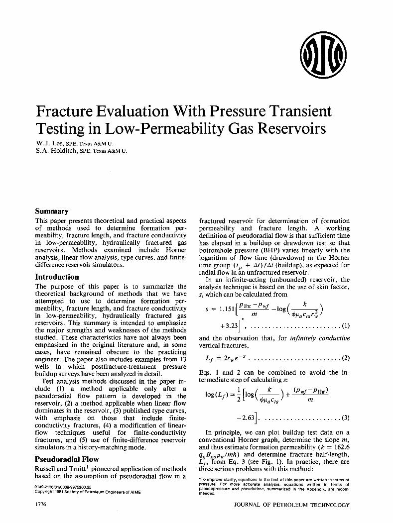
In principle, we can plot buildup test data on a conventional Horner graph, determine the slope m, and thus estimate formation permeability (k = 162.6 qgBg"al1a1mh) and determine fracture half-length, L j , from Eq. 3 (see Fig. 1). In practice, there are tliree serious problems with this method:

°To improve clarity, equations in the text of this paper are written in terms of pressure. For more accurate analysis, equations written in terms of pseudopressure and pseudotime, summarized in the Appendix, are recom· mended.

JOURNAL OF PETROLEUM TECHNOLOGY

8000

Pi = 7650

7000

6000 ~ c.

~

c.~

5000

4000

100 10

Fig. 1 - Horner plot, pressure buildup test data, south Texas gas well.

1. The time required to reach the required straight line where the slope is related to formation perme­ability can be impractically long (months or years) in low-permeability gas reservoirs with long fractures, as demonstrated by Gringarten et af.2 and Cinco et af. 3

2. Implicit in the method is the assumption of infinite fracture conductivity, which is not always valid. 4

3. By the time the pressure transient has moved beyond the region of the reservoir influenced by the fractures, effects of the reservoir boundary already may have become important, preventing develop­ment of the proper slope, m.

Russell and Truitt developed a technique for overcoming Limitation 3. While we have not found their proposal to be of direct value in dealing with low-permeability gas reservoirs, we have found that a related technique offers promise for estimating fracture length and formation permeability from limited-duration buildup test data. This technique involves a trial-and-error process of (1) determining the maximum slope on a Horner plot; (2) estimating an apparent formation permeability from this slope; (3) calculating the ratio of true-to-apparent per­meability, ktlka' from a theoretically derived correlation that requires knowledge of fracture length; (4) estimating fracture length using a square­root-of-time graph; and (5) iterating to convergence. Applicability of this method to finite-conductivity fractures has been demonstrated by Holditch et af. 5

In summary, the major limitation of the standard Russell and Truitt method (Eq. 3) is that it is rarely applicable to low-permeability, fractured gas reser­voirs because of the long times required to establish the straight line where the slope is related to the for­mation permeability.

Linear Flow Millheim and Cichowicz6 showed that when linear

SEPTEMBER 1981

flow into a fracture dominates (at earliest times) in a drawdown test, pressure/time behavior is modeled by

, Y2 _ qgBga (~)Y2=m tp .

Pi-Pwf-4.064 hLf

k(jJcta

............................. (4)

For a buildup test, with linear flow continuing to time tp + t::.t,

Pi -Pws =m' (.Jtp + t::.t -.Jffi) . ........... (5)

Further, when t p > > t::.t,

P ws - P wf == m' .Jffi. . .................. (6)

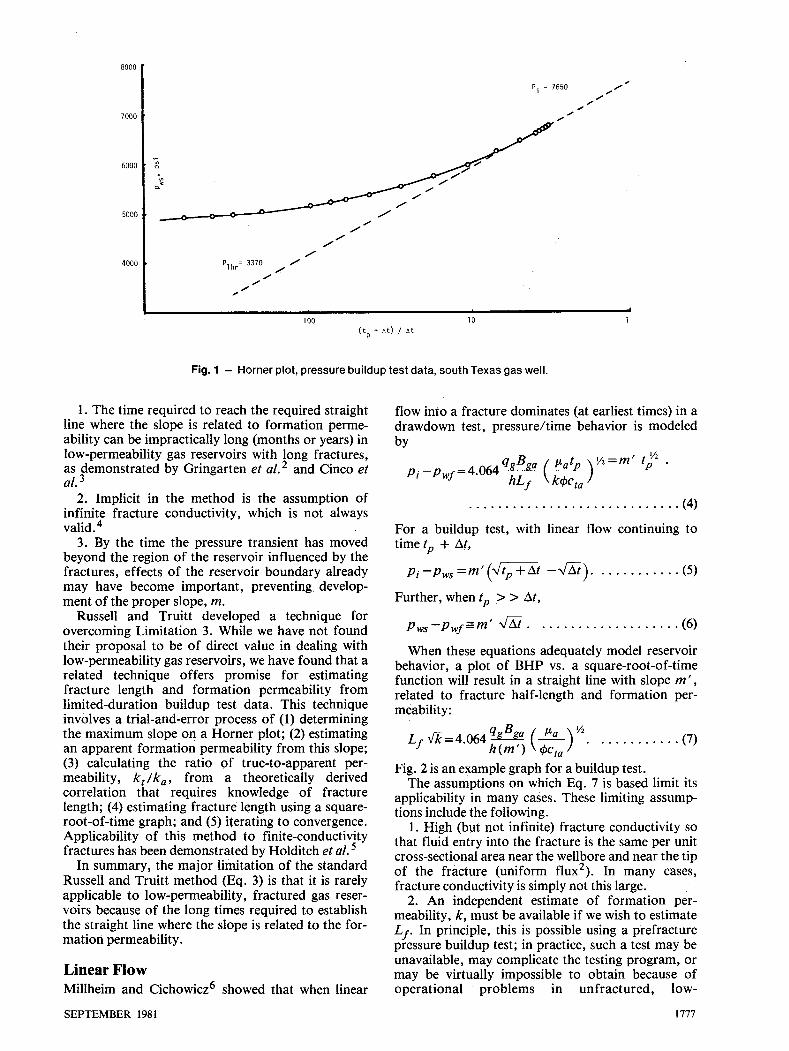
When these equations adequately model reservoir behavior, a plot of BHP vs. a square-root-of-time function will result in a straight line with slope m' , related to fracture half-length and formation per­meability:

Lf

Yk = 4.064 qgBga (~) Y2. . ...•...... (7) h(m') (jJCta

Fig. 2 is an example graph for a buildup test. The assumptions on which Eq. 7 is based limit its

applicability in many cases. These limiting assump­tions include the following.

1. High (but not infinite) fracture conductivity so that fluid entry into the fracture is the same per unit cross-sectional area near the well bore and near the tip of the fracture (uniform flux 2). In many cases, fracture conductivity is simply not this large.

2. An independent estimate of formation per­meability, k, must be available if we wish to estimate Lf . In principle, this is possible using a prefracture pressure buildup test; in practice, such a test may be unavailable, may complicate the testing program, or may be virtually impossible to obtain because of operational problems in unfractured, low-

1777

7800

7000

]0

Fig. 2 - Millheim-Cichowicz plot, pressure buildup test data, south Texas gas well.

permeability gas wells. 3. Application of the method to earliest-time data,

which may be dominated by linear flow, requires absence of well bore storage distortion. Unfortu­nately, well bore storage can distort data for a signifi­cant time period in some low-permeability fractured gas wells.

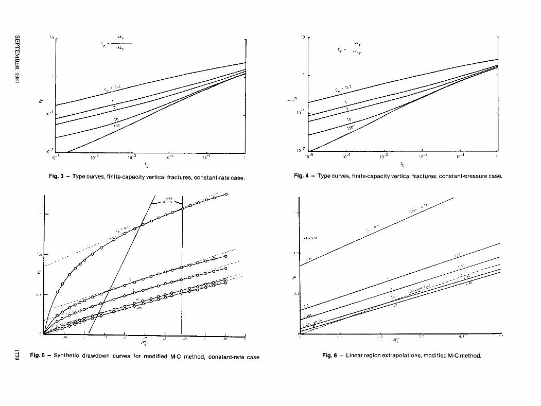
Type Curves Several type curves2,3,7,8 have potential application to analysis of transient tests in low-permeability, fractured gas reservoirs. Particularly important are Cinco et al. 's3 curves for finite-conductivity frac­tures, constant-rate case (Fig. 3) and Agarwal et al.'s8 curves for finite-conductivity fractures, constant-bottomhole-pressure case. (Fig. 4 shows a similar curve we have generated for use in our research work.) Even these curves, however, are based on assumptions that are sometimes limiting, such as negligible well bore storage distortion and infinite-acting reservoirs. To include these variables and finite-conductivity on a single type curve probably would be impractically complex, yet these effects can be important and can be misinterpreted.

In principle, if we place data in the position of best fit on the Cinco et al. or Agarwal et al. type curves, we can determine simultaneously (and uniquely) reservoir permeability, k, fracture half-length, L r, and fracture conductivity, wkj . Unfo~tunately, the position of best fit is not always ObVlOUS; thIS can lead to a multiplici~ of possible formation and fracture descriptions. As Agarwal et al. 8 point out, the uniqueness problem is diminished considerably if we know formation permeability independently (from a prefracture buildup test, for example) but, as we noted earlier, a prefracture buildup may be most difficult to run or it may be too late when we recognize the need for the information.

Another problem with application of type curves

1778

to buildup tests is that most type curves (including those of Cinco et al. and Agarwal et al.) were developed for use with drawdown tests in which we plot log (Pi - Pwj) vs. log t. They are applicable to buildup tests if we plot log (P ws - Pwj) vs. log !1t when and only when producing time, t p' before t~e buildup test is large compared with maXImum shut-m time analyzed in the buildup test. Unfortunately, production and shut-in periods are often of com­parable magnitude in testin~ programs. for low­permeability gas wells, makmg conventIOnal type curves inapplicable unless the values of !1t are

I 10 corrected for t p' as suggested by Agarwa .

Modified Millheim-Cichowicz Method

We have found a modification of the square-root-of­time plot, as suggested by Millheim and Cichowicz,6

to be helpful in estimating fracture properties; we call this technique the modified M-C method. The method is based on a plot of dimensionless pressure vs. the square root of dimensionless time for finite­conductivity vertical fractures. For large values of fracture conductivity (characterized by the dimen­sionless fracture-conductivity parameter, 0 = wkf l1rkL j), Pi - Pwj is a linear function of v t with an intercept near zero. For lower values of Cr (more pressure drop in the fracture), a plot of Pi - Pwj vs. Ytis nonlinear at earliest times. There is a later lInear portion; however, the intercept is far from zero. We have found that the intercept is related uniquely to dimensionless fracture conductivity.

Fig. 5 illustrates the character of this type of plot. This figure is simply a plot of the data published by Cinco et al. 5 for constant producing rate in the form ofPD vs. -Jt;;, where

kh(Pi-Pwj) PD= , .................. (8)

141.2 qgBgaP-a

JOURNAL OF PETROLEUM TECHNOLOGY

V1 10 wk f 10 l"!'l

'" Cr ---- wk f .., nkL

f l"!'l C ~

~ ~

r

t:1:I l"!'l :;tI

:0 00

,f' '0

~Icr

10-1 10-1

Fig_ 3 - Type curves, finite-capacity vertical fractures, constant-rate case. Fig. 4 - Type curves, finite-capacity vertical fractures, constant-pressure case.

,5

Fig. 5 - Synthetic drawdown curves for modified M-e method, constant-rate case. Fig. 6 - Linear region extrapolations, modified M-e method.

0.5

UNIFORM FLUX

0.4 INFINITE CONDUCTIVITY

~ 0.3

0.2

0.1

0.1 0.2 0.3

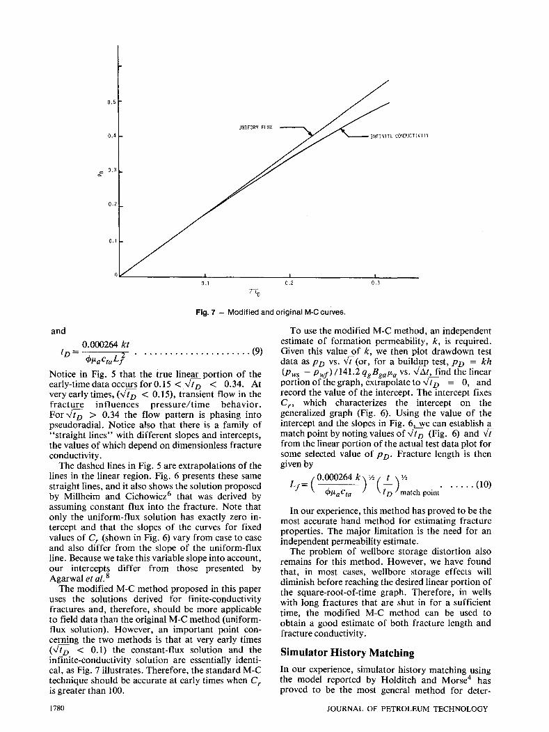
Fig. 7 - Modified and original M·e curves.

and

0.000264 kt tD = 2 ••.•.•...•••.•.•••.... (9)

¢Jl-taCtaLf

Notice in Fig. 5 that the true linear portion of the early-time data occurs for 0.15 < -.It;; < 0.34. At very early times, (-.It;; < 0.15), transient flow in the fracture influences pressure/time behavior. For -.It;; > 0.34 the flow pattern is phasing into pseudo radial. Notice also that there is a family of "straight lines" with different slopes and intercepts, the values of which depend on dimensionless fracture conductivity.

The dashed lines in Fig. 5 are extrapolations of the lines in the linear region. Fig. 6 presents these same straight lines, and it also shows the solution proposed by Millheim and Cichowicz6 that was derived by assuming constant flux into the fracture. Note that only the uniform-flux solution has exactly zero in­tercept and that the slopes of the curves for fixed values of C, (shown in Fig. 6) vary from case to case and also differ from the slope of the uniform-flux line. Because we take this variable slope into account, our intercepts differ from those presented by Agarwal et at. 8

The modified M-C method proposed in this paper uses the solutions derived for finite-conductivity fractures and, therefore, should be more applicable to field data than the original M-C method (uniform­flux solution). However, an important point con­cerning the two methods is that at very early times (-.It;; < 0.1) the constant-flux solution and the infinite-conductivity solution are essentially identi­cal, as Fig. 7 illustrates. Therefore, the standard M-C technique should be accurate at early times when C, is greater than 100.

1780

To use the modified M-C method, an independent estimate of formation permeability, k, is required. Given this value of k, we then plot drawdown test data as PD vs. Vt (or, for a build!!Q test, PD = kh (P ws - Pwf) /141.2 qgBgal-ta vs. Yilt, find the linear portion of the graph, extrapolate to -.It;; = 0, and record the value of the intercept. The intercept fixes C" which characterizes the intercept on the generalized graph (Fig. 6). Using the value of the intercept and the slopes in Fig. 6, we can establish a match point by noting values of -.It;; (Fig. 6) and Vt from the linear portion of the actual test data plot for some selected value of PD. Fracture length is then given by

(0.000264 k)!h ( t ) Y2

Lf = - ...... (10) ¢Jl-taCta tD match point

In our experience, this method has proved to be the most accurate hand method for estimating fracture properties. The major limitation is the need for an independent permeability estimate.

The problem of wellbore storage distortion also remains for this method. However, we have found that, in most cases, well bore storage effects will diminish before reaching the desired linear portion of the square-root-of-time graph. Therefore, in wells with long fractures that are shut in for a sufficient time, the modified M-C method can be used to obtain a good estimate of both fracture length and fracture conductivity.

Simulator History Matching

In our experience, simulator history matching using the model reported by Holditch and Morse4 has proved to be the most general method for deter-

JOURNAL OF PETROLEUM TECHNOLOGY

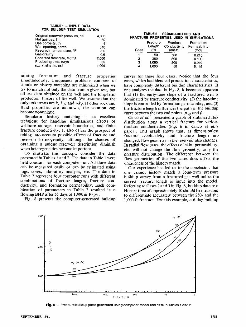
TABLE 1 - INPUT DATA FOR BUILDUP TEST SIMULATION

Original reservoir pressure, psi Net gas pay, ft Gas porosity, % Well spacing, acres Reservoir temperature, 0 F Gas gravity Constant flow rate, Mcf/D Producing time, days Pwf at shut in, psi

4,000 50

4 640 200 0.6

2,000 55

1,990

mining formation and fracture properties simultaneously. Uniqueness problems common to simulator history matching are minimized when we try to match not only the data from a given test, but all test data obtained on the well and the long-term production history of the well. We assume that the only unknowns are k, L j' and wk j' If other rock and fluid properties are unknown, the solution can become nonunique.

Simulator history matching is an excellent technique for handling simultaneous effects of well bore storage, reservoir boundaries, and finite fracture conductivity. It also offers the prospect of taking into account possible effects of fracture and reservoir heterogeneity, although the chances of obtaining a unique reservoir description diminish when heterogeneities become important.

To illustrate this concept, consider the data presented in Tables 1 and 2. The data in Table 1 were held constant for each computer run. All these data can be measured easily or can be estimated using logs, cores, laboratory analysis, etc. The data in Table 2 represent four computer runs with different combinations of fracture length, fracture con­ductivity, and formation permeability. Each com­bination of parameters in Table 2 resulted in a flowing BHP after 55 days of 1,990 ± 10 psi.

Fig. 8 presents the computer-generated buildup

4000

3000

wk f (md-ft)

2000 L-===::::::::::~:::'====::::::::::::::'----

10000 1000

TABLE 2 - PERMEABILITIES AND FRACTURE PROPERTIES USED IN SIMULATIONS

Case

1 2 3 4

Fracture Length

(tt)

50 250

1,000 1,000

Fracture Conductivity

(md-tt)

500 500 500

50

Formation Permeability

(md)

0.215 0.100 0.019 0.115

curves for these four cases. Notice that the four cases, which had identical production characteristics, have completely different buildup characteristics. If one analyzes the data in Fig. 8, it becomes apparent that (1) the early-time slope of a fractured well is dominated by fracture conductivity, (2) the late-time slope is controlled by formation permeability, and (3) the fracture length influences the path of the buildup curve between the two end points, P wf and jJ.

Cinco et al. 3 presented a graph of stabilized flux distribution along a vertical fracture for various fracture conductivities (Fig. 6 in Cinco et al. 's paper). This graph shows that, as dimensionless fracture conductivity and fracture length are changed, flow geometry in the reservoir also changes. In radial flow cases, the effects of skin, permeability, etc. will not change the flow geometry, only the pressure distribution. The difference between the flow geometries of the two cases does affect the uniqueness of the history match.

Our experience has led us to the conclusion that one cannot history match a long-term pressure buildup survey from a fractured gas well unless the correct fracture length is input into the model. Referring to Cases 2 and 3 in Fig. 8, buildup data to a Horner time of approximately 10 should be measured to differentiate accurately between the 250- and the 1,000-ft fracture. For this example, a 6-day buildup

Run

100 10 (t .. H) / lit

Fig. 8 - Pressure buildup plots generated using computer model and data in Tables 1 and 2.

SEPTEMBER 1981 1781

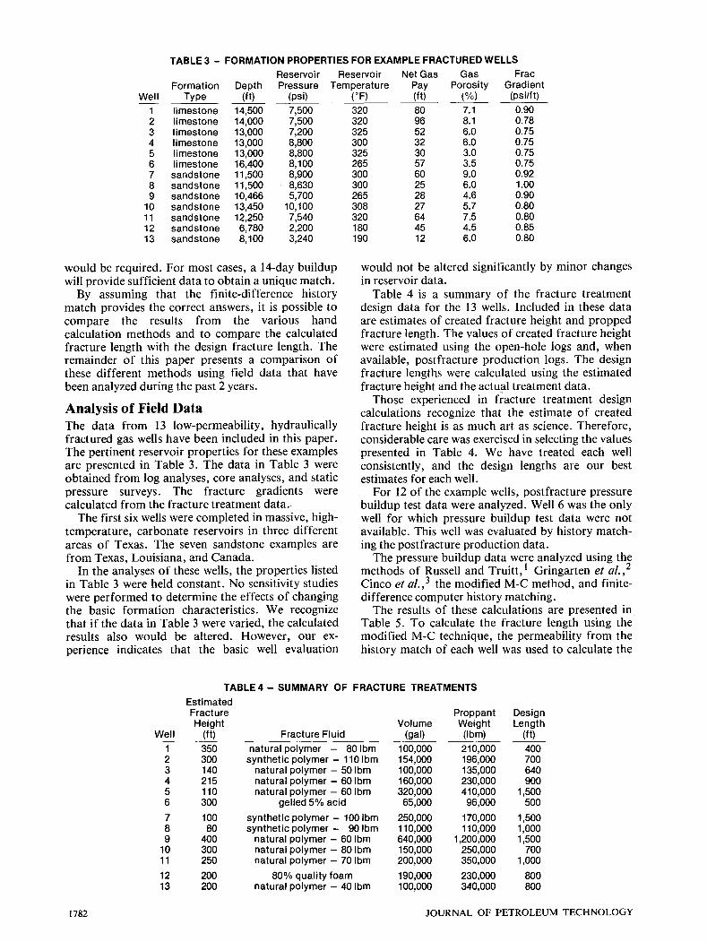
TABLE 3 - FORMATION PROPERTIES FOR EXAMPLE FRACTURED WELLS

Reservoir Reservoir Net Gas Gas Frac Formation Depth Pressure Temperature Pay Porosity Gradient

Well Type (tt) (psi) -

1 limestone 14,500 7,500 2 limestone 14,000 7,500 3 limestone 13,000 7,200 4 limestone 13,000 8,800 5 limestone 13,000 8,800 6 limestone 16,400 8,100 7 sandstone 11,500 8,900 8 sandstone 11,500 8,630 9 sandstone 10,466 5,700

10 sandstone 13,450 10,100 11 sandstone 12,250 7,540 12 sandstone 6,780 2,200 13 sandstone 8,100 3,240

would be required. For most cases, a 14-day buildup will provide sufficient data to obtain a unique match.

By assuming that the finite-difference history match provides the correct answers, it is possible to compare the results from the various hand calculation methods and to compare the calculated fracture length with the design fracture length. The remainder of this paper presents a comparison of these different methods using field data that have been analyzed during the past 2 years.

Analysis of Field Data The data from 13 low-permeability, hydraulically fractured gas wells have been included in this paper. The pertinent reservoir properties for these examples are presented in Table 3. The data in Table 3 were obtained from log analyses, core analyses, and static pressure surveys. The fracture gradients were calculated from the fracture treatment data.

The first six wells were completed in massive, high­temperature, carbonate reservoirs in three different areas of Texas. The seven sandstone examples are from Texas, Louisiana, and Canada.

In the analyses of these wells, the properties listed in Table 3 were held constant. No sensitivity studies were performed to determine the effects of changing the basic formation characteristics. We recognize that if the data in Table 3 were varied, the calculated results also would be altered. However, our ex­perience indicates that the basic well evaluation

(OF) (tt) (%) (psi/tt)

320 80 7.1 0.90 320 96 8.1 0.78 325 52 6.0 0.75 300 32 6.0 0.75 325 30 3.0 0.75 265 57 3.5 0.75 300 60 9.0 0.92 300 25 6.0 1.00 265 28 4.6 0.90 308 27 5.7 0.80 320 64 7.5 0.80 180 45 4.5 0.85 190 12 6.0 0.80

would not be altered significantly by minor changes in reservoir data.

Table 4 is a summary of the fracture treatment design data for the 13 wells. Included in these data are estimates of created fracture height and propped fracture length. The values of created fracture height were estimated using the open-hole logs and, when available, post fracture production logs. The design fracture lengths were calculated using the estimated fracture height and the actual treatment data.

Those experienced in fracture treatment design calculations recognize that the estimate of created fracture height is as much art as science. Therefore, considerable care was exercised in selecting the values presented in Table 4. We have treated each well consistently, and the design lengths are our best estimates for each well.

For 12 of the example wells, post fracture pressure buildup test data were analyzed. Well 6 was the only well for which pressure buildup test data were not available. This well was evaluated by history match­ing the post fracture production data.

The pressure buildup data were analyzed using the methods of Russell and Truitt,l Gringarten et aI., 2

Cinco et al., 3 the modified M-C method, and finite­difference computer history matching.

The results of these calculations are presented in Table 5. To calculate the fracture length using the modified M-C technique, the permeability from the history match of each well was used to calculate the

TABLE 4 - SUMMARY OF FRACTURE TREATMENTS

Estimated Fracture Proppant Design Height Volume Weight Length

Well (tt) Fracture Fluid (gal) (Ibm) (tt) -

1 350 natural polymer - 80 Ibm 100,000 210,000 400 2 300 synthetic polymer - 110 Ibm 154,000 196,000 700 3 140 natural polymer - 50 Ibm 100,000 135,000 640 4 215 natural polymer - 60 Ibm 160,000 230,000 900 5 110 natural polymer - 60 Ibm 320,000 410,000 1,500 6 300 gelled 5% acid 65,000 96,000 500

7 100 synthetic polymer - 100 Ibm 250,000 170,000 1,500 8 80 synthetic polymer - 90 Ibm 110,000 110,000 1,000 9 400 natural polymer - 60 Ibm 640,000 1,200,000 1,500

10 300 natural polymer - 80 Ibm 150,000 250,000 700 11 250 natural polymer - 70 Ibm 200,000 350,000 1,000

12 200 80% quality foam 190,000 230,000 800 13 200 natural polymer - 40 Ibm 100,000 340,000 800

1782 JOURNAL OF PETROLEUM TECHNOLOGY

dimensionless pressures. As discussed earlier, the results from the finite­

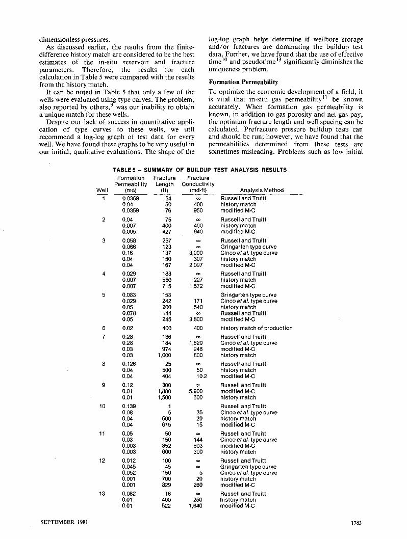
difference history match are considered to be the best estimates of the in-situ reservoir and fracture parameters. Therefore, the results for each calculation in Table 5 were compared with the results from the history match.

It can be noted in Table 5 that only a few of the wells were evaluated using type curves. The problem, also reported by others,9 was our inability to obtain a unique match for these wells.

Despite our lack of success in quantitative appli­cation of type curves to these wells, we still recommend a log-log graph of test data for every well. We have found these graphs to be very useful in our initial, qualitative evaluations. The shape of the

log-log graph helps determine if well bore storage and/or fractures are dominating the buildup test data. Further, we have found that the use of effective time 10 and pseudotime 13 significantly diminishes the uniqueness problem.

Formation Permeability

To optimize the economic development of a field, it is vital that in-situ gas permeabilityll be known accurately. When formation gas permeability is known, in addition to gas porosity and net gas pay, the optimum fracture length and well spacing can be calculated. Prefracture pressure buildup tests can and should be run; however, we have found that the permeabilities determined from these tests are sometimes misleading. Problems such as low initial

TABLES - SUMMARY OF BUILDUP TEST ANALYSIS RESULTS

Formation Fracture Fracture Permeability Length Conductivity

Well (md) (tt) (md·ft) Analysis Method -

1 0.0359 54 00 Russell and Truitt 0.04 50 400 history match 0.0359 76 950 modified M·C

2 0.04 75 00 Russell and Truitt 0.007 400 400 history match 0.005 427 940 modified MoC

3 0.058 257 00 Russell and Truitt 0.066 123 00 Gringarten type curve 0.16 137 3,000 Cinco et al. type curve 0.04 150 307 history match 0.04 167 2,097 modified M·C

4 0.029 183 00 Russell and Truitt 0.007 550 227 history match 0.007 715 1,572 modified M·C

5 0.083 153 Gringarten type curve 0.029 242 171 Cinco et al. type curve 0.05 200 540 history match 0.Q78 144 00 Russell and Truitt 0.05 245 3,800 modified M·C

6 0.02 400 400 history match of production

7 0.28 136 00 Russell and Truitt 0.28 184 1,620 Cinco et al. type curve 0.03 974 948 modified M·C 0.03 1,000 800 history match

8 0.126 25 00 Russell and Truitt 0.04 500 50 history match 0.04 404 10.2 modified M·C

9 0.12 300 00 Russell and Truitt 0.01 1,880 5,900 modified M·C 0.01 1,500 500 history match

10 0.139 1 Russell and Truitt 0.08 5 35 Cinco et al. type curve 0.04 500 20 history match 0.04 615 15 modified MoC

11 0.05 50 00 Russell and Truitt 0.03 150 144 Cinco et al. type curve 0.003 852 803 modified M·C 0.003 600 300 history match

12 0.012 100 00 Russell and Truitt 0.045 45 00 Gringarten type curve 0.052 150 5 Cinco et al. type curve 0.001 700 20 history match 0.001 829 260 modified MoC

13 0.082 16 00 Russell and Truitt 0.01 400 250 history match 0.01 522 1,640 modified MoC

SEPTEMBER 1981 1783

E ,g ~ :0 co Q)

E Qi a. :c o iii E ~ o Cii :c E e.~ _rJl >.z,

:!::<tS ._ c:: .DCO CO ... Q)Q) Ec:: Qio a.J:

1.0 •

.3

• • .6

.4

.1

.001 .01 10

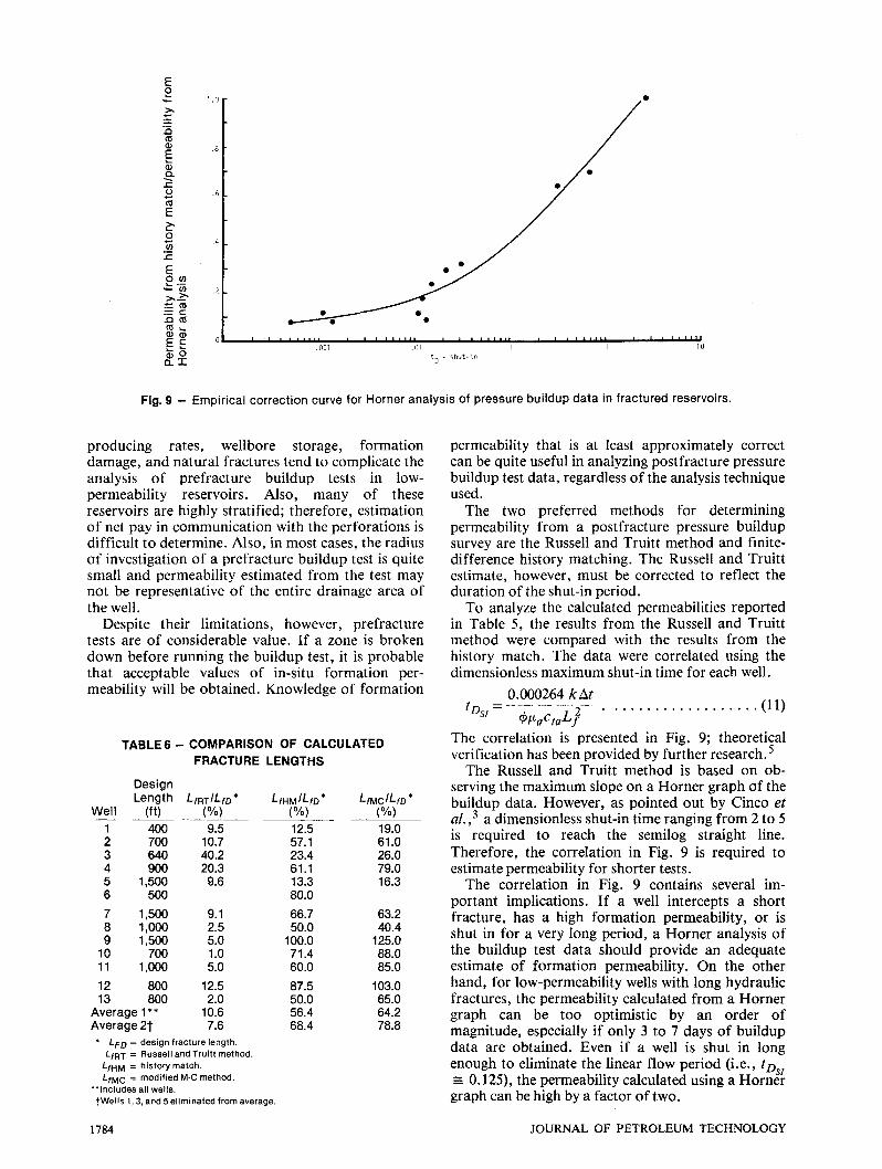
Fig. 9 - Empirical correction curve for Horner analysis of pressure buildup data in fractured reservoirs.

producing rates, well bore storage, formation damage, and natural fractures tend to complicate the analysis of prefracture buildup tests in low­permeability reservoirs. Also, many of these reservoirs are highly stratified; therefore, estimation of net pay in communication with the perforations is difficult to determine. Also, in most cases, the radius of investigation of a pre fracture buildup test is quite small and permeability estimated from the test may not be representative of the entire drainage area of the well.

Despite their limitations, however, prefracture tests are of considerable value. If a zone is broken down before running the buildup test, it is probable that acceptable values of in-situ formation per­meability will be obtained. Knowledge of formation

TABLE 6 - COMPARISON OF CALCULATED FRACTURE LENGTHS

Design Length LfAT/LtD ' LfHM/LfD' LfMC/LtD '

Well ~ (%) (%) (%)

1 400 9.5 12.5 19.0 2 700 10.7 57.1 61.0 3 640 40.2 23.4 26.0 4 900 20.3 61.1 79.0 5 1,500 9.6 13.3 16.3 6 500 80.0

7 1,500 9.1 66.7 63.2 8 1,000 2.5 50.0 40.4 9 1,500 5.0 100.0 125.0

10 700 1.0 71.4 88.0 11 1,000 5.0 60.0 85.0

12 800 12.5 87.5 103.0 13 800 2.0 50.0 65.0

Average 1" 10.6 56.4 64.2 Average2t 7.6 68.4 78.8

LFD = design fracture length. LfRT = Russell and Truitt method.

LfHM = history match. LfMC = modified M·C method.

""Includes all wells. tWel!s 1, 3, and 5 eliminated from average.

1784

permeability that is at least approximately correct can be quite useful in analyzing post fracture pressure buildup test data, regardless of the analysis technique used.

The two preferred methods for determining permeability from a post fracture pressure buildup survey are the Russell and Truitt method and finite­difference history matching. The Russell and Truitt estimate, however, must be corrected to reflect the duration of the shut-in period.

To analyze the calculated permeabilities reported in Table 5, the results from the Russell and Truitt method were compared with the results from the history match. The data were correlated using the dimensionless maximum shut-in time for each well.

0.000264 k fit ---"2-' .................. (11)

¢J.taCtaLj

The correlation is presented in Fig. 9; theoretical verification has been provided by further research. 5

The Russell and Truitt method is based on ob­serving the maximum slope on a Horner graph of the buildup data. However, as pointed out by Cinco et al., 3 a dimensionless shut-in time ranging from 2 to 5 is required to reach the semilog straight line. Therefore, the correlation in Fig. 9 is required to estimate permeability for shorter tests.

The correlation in Fig. 9 contains several im­portant implications. If a well intercepts a short fracture, has a high formation permeability, or is shut in for a very long period, a Horner analysis of the buildup test data should provide an adequate estimate of formation permeability. On the other hand, for low-permeability wells with long hydraulic fractures, the permeability calculated from a Horner graph can be too optimistic by an order of magnitude, especially if only 3 to 7 days of buildup data are obtained. Even if a well is shut in long enough to eliminate the linear flow period (i.e., tD == 0.125), the permeability calculated using a HornJf graph can be high by a factor of two.

JOURNAL OF PETROLEUM TECHNOLOGY

Fracture Length Table 6 presents a comparison of fracture lengths calculated using the different analysis methods. All calculated lengths have been normalized with respect to the design length. Two averages have been presented for each technique. Average 1 includes the ratios for every well. Average 2 was prepared by eliminating the values for Wells 1, 3, and 5. These three wells obviously contained short fractures, probably caused by poor sand transport; they are discussed in more detail later. Therefore, Average 2 is believed to be more representative of a typical treatment.

The fracture lengths calculated using the Russell and Truitt method averaged only 5% to 11070 of the designed fracture lengths. The history-match fracture lengths averaged about 68% of the designed lengths. The fracture lengths calculated using the modified M-C technique averaged about 79% of the design lengths. It must be remembered, however, that the fracture lengths calculated using the modified M-C method are based on the formation permeability as determined from the history match.

An analysis of the data in Table 6 leads to several important observations. If one assumes that the history match is correct, the average treatment only achieves about 70% of the design length. This ob­servation implies that (1) the actual fracture is wider -and shorter than predicted by the conventional design equations, (2) sand transport in the fracture is not as efficient as expected, (3) fluid loss in the fracture is larger than predicted using conventional techniques, (4) the barriers that control fracture height are routinely underestimated, or (5) there is some other, less obvious, reason. The important point is that for the examples in this paper, only 70% of the design length was achieved during the fracture treatment.

Three of the examples, Wells 1, 3, and 5, ap­parently do not contain long hydraulic fractures. In Tables 1 and 2, it can be seen that all three wells were completed in deep, massive, high-temperature limestone reservoirs. For these three wells, detailed analyses of the fracture treatment data indicated that two problems existed. First, good barriers to fracture growth were not obvious from the logs and second, the gel concentrations were low, which may have allowed the sand to settle below the gas pay during the treatment.

On the basis of these observations and similar observations by various operators in these same areas, recent treatments have used higher gel con­centrations, smaller-mesh propp ants , and density­controlled treatments. 12 It was apparent from the analysis of Wells 1, 3, and 5 that long fractures were being created, and large volumes of proppant were being pumped; but the fracture opposite the pay zone was not being propped. The emphasis on sand transport that resulted from the analyses of these three wells has helped to define a problem and, it is hoped, future wells in such reservoirs can be stimulated more effectively.

SEPTEMBER 1981

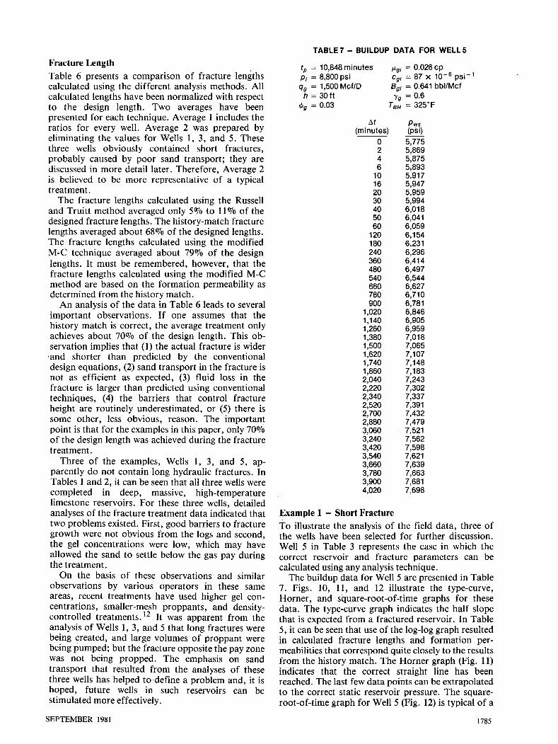
TABLE 7 - BUILDUP DATA FOR WELL 5

tp = 10,848 minutes Pi = 8,800 psi qg = 1,500 Mcf/D h=30ft

cJ>g = 0.03

flt (minutes)

o 2 4 6

10 16 20 30 40 50 60

120 180 240 360 480 540 660 780 900

1,020 1,140 1,260 1,380 1,500 1,620 1,740 1,860 2,040 2,220 2,340 2,520 2,700 2,880 3,060 3,240 3,420 3,540 3,660 3,780 3,900 4,020

/J-gi = 0.026 cp Cgi = 87 X 10- 6 psi- 1

Bgi = 0.641 bbl/Mcf 'Yg = 0.6

TBH = 325°F

Pws (psi)

5,775 5,869 5,875 5,893 5,917 5,947 5,959 5,994 6,018 6,041 6,059 6,154 6,231 6,296 6,414 6,497 6,544 6,627 6,710 6,781 6,846 6,905 6,959 7,018 7,065 7,107 7,148 7,183 7,243 7,302 7,337 7,391 7,432 7,479 7,521 7,562 7,598 7,621 7,639 7,663 7,681 7,698

Example 1 - Short }'racture To illustrate the analysis of the field data, three of the wells have been selected for further discussion. Well 5 in Table 3 represents the case in which the correct reservoir and fracture parameters can be calculated using any analysis technique.

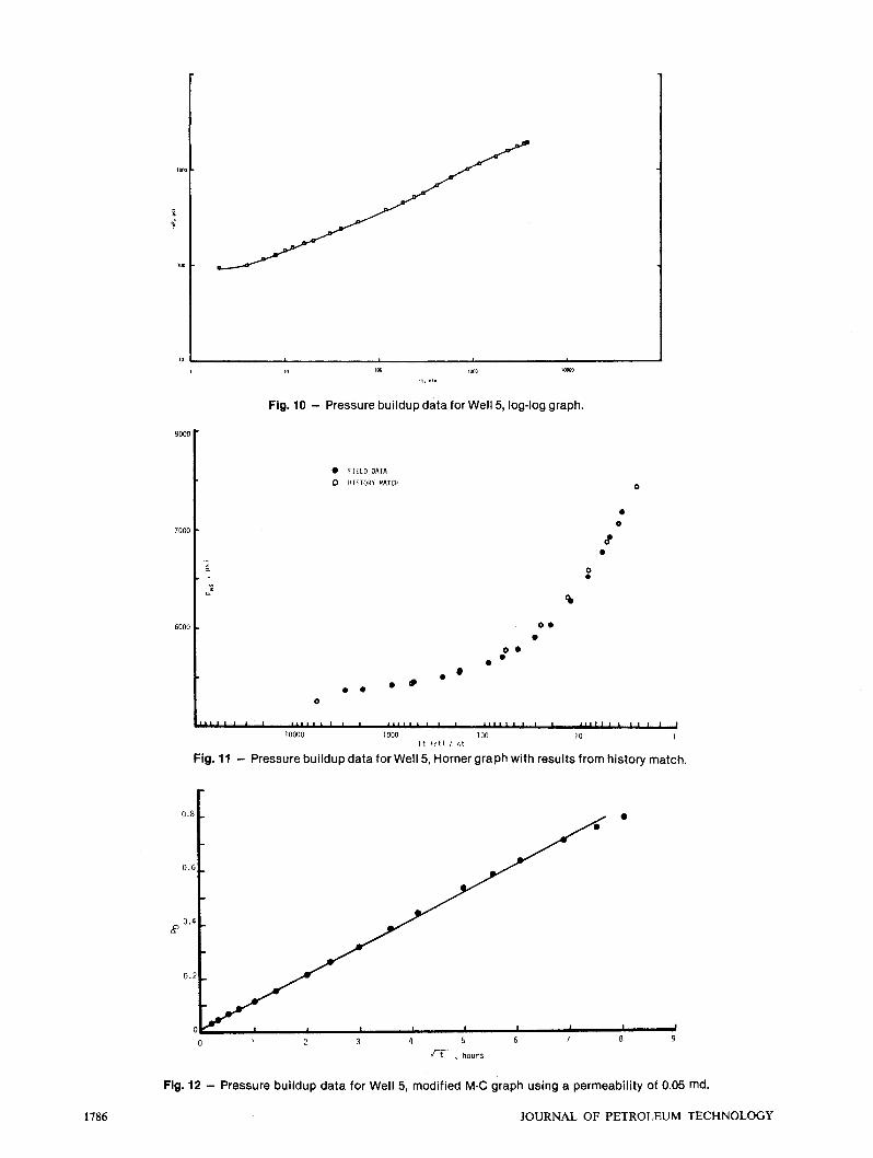
The buildup data for Well 5 are presented in Table 7. Figs. 10, 11, and 12 illustrate the type-curve, Horner, and square-root-of-time graphs for these data. The type-curve graph indicates the half slope that is expected from a fractured reservoir. In Table 5, it can be seen that use of the log-log graph resulted in calculated fracture lengths and formation per­meabilities that correspond quite closely to the results from the history match. The Horner graph (Fig. 11) indicates that the correct straight line has been reached. The last few data points can be extrapolated to the correct static reservoir pressure. The square­root-of-time graph for Well 5 (Fig. 12) is typical of a

1785

1786

1000

8000

7000

6000

rr

c!

,,0' ","" H.llin

Fig. 10 - Pressure buildup data for Well 5, log-log graph_

• fIELD DATA

o HISTORY MATCH

• • . -o

10000 1000

• • •

100 (t +6t) / At

o • •

o.

•

10

o •

~ •

• o

o

Fig. 11 - Pressure buildup data for Well 5, Horner graph with results from history match .

•

rt . hours

Fig. 12 - Pressure buildup data for Well 5, modified M-e graph using a permeability of 0.05 md.

JOURNAL OF PETROLEUM TECHNOLOGY

well that contains a short, highly conductive fracture. The data form a straight line that can be extrapolated to a dimensionless pressure of approximately zero.

Each analysis technique applied to this case led to consistent results. Using the history-match values of 0.05 md, a 2oo-ft fracture, and 4,000 minutes of shut-in time, the dimensionless shut-in time was calculated to be about 2.6. Therefore, the reliability of the Russell and Truitt analysis is confirmed for this well.

In Table 4, it can be seen that the fracture treat­ment for Well 5 was designed for 110 ft of created fracture height. The actual treatment consisted of 320,000 gal of a 60-lbm gel carrying 410,000 Ibm of propping agent. This size treatment should have resulted in a propped fracture of 1,500 ft. It becomes obvious that (1) the created fracture height was probably much greater than the 110 ft used in the design calculations, and/or (2) the 60-lbm gel in the 325°F reservoir did not maintain enough viscosity to transport the propp ant as required. These con­clusions concerning Well 5 were used to improve the fracture treatment designs in this area. Recent treatments by several operators have used sub­stantially more gel and smaller-mesh proppants to improve the sand transport capabilities ofthe fluid.

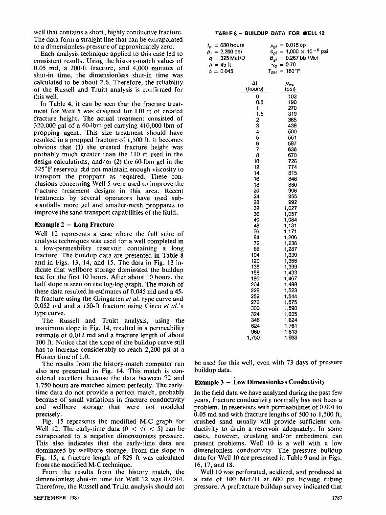
Example 2 - Long Fracture Well 12 represents a case where the full suite of analysis techniques was used for a well completed in a low-permeability reservoir containing a long fracture. The buildup data are presented in Table 8 and in Figs. 13, 14, and 15. The data in Fig. 13 in­dicate that well bore storage dominated the buildup test for the first 10 hours. After about 10 hours, the half slope is seen on the log-log graph. The match of these data resulted in estimates of 0.045 md and a 45-ft fracture using the Gringarten et af. type curve and 0.052 md and a 150-ft fracture using Cinco et af.'s type curve.

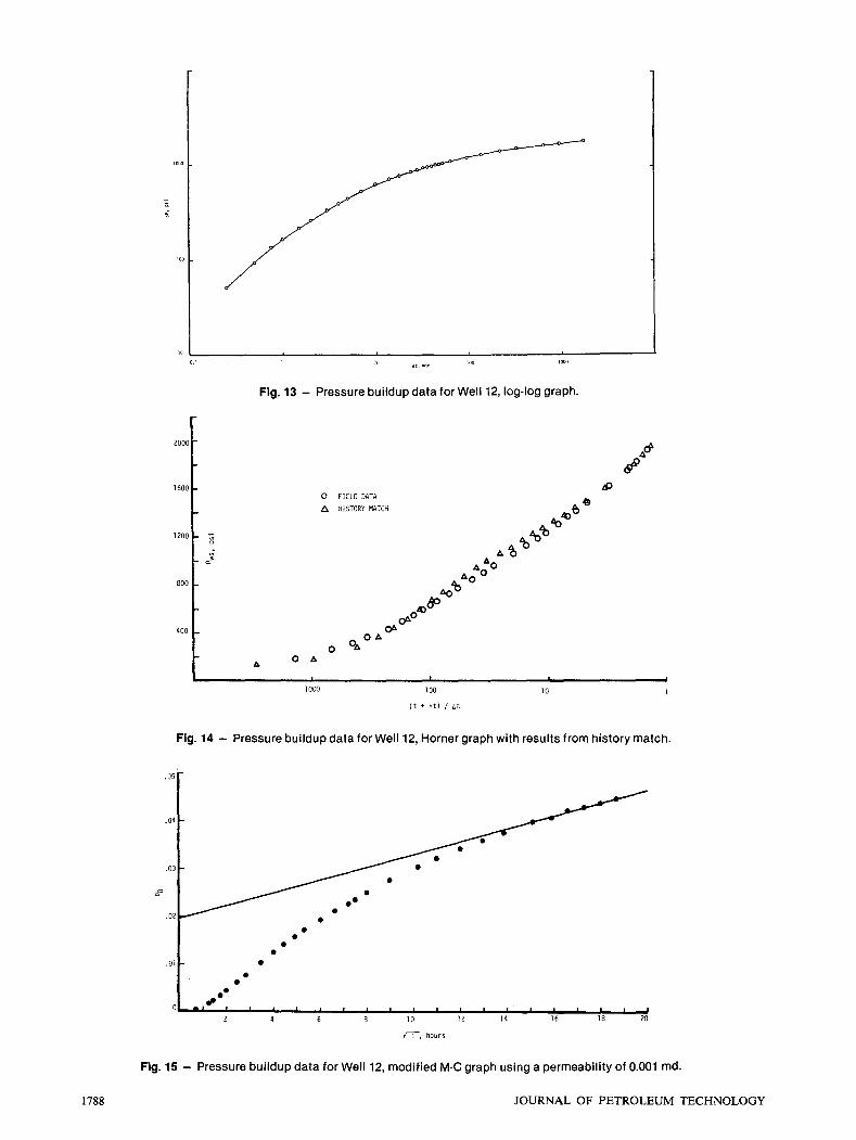
The Russell and Truitt analysis, using the maximum slope in Fig. 14, resulted in a permeability estimate of 0.012 md and a fracture length of about 100 ft. Notice that the slope of the buildup curve still has to increase considerably to reach 2,200 psi at a Horner time of 1.0.

The results from the history-match computer run also are presented in Fig. 14. This match is con­sidered excellent because the data between 72 and 1,750 hours are matched almost perfectly. The early­time data do not provide a perfect match, probably because of small variations in fracture conductivity and well bore storage that were not modeled precisely.

Fig. 15 represents the modified M-C graph for Well 12. The early-time data (0 < VI < 5) can be extrapolated to a negative dimensionless pressure. This also indicates that the early-time data are dominated by well bore storage. From the slope in Fig. 15, a fracture length of 829 ft was calculated from the modified M-C technique.

From the results from the history match, the dimensionless shut-in time for Well 12 was 0.0014. Therefore, the Russell and Truitt analysis should not

SEPTEMBER 1981

TABLE 8 - BUILDUP DATA FOR WELL 12

tp = 680 hours Pi = 2,200 psi q = 325 Mcf/D h = 45ft

cJ> = 0.045

Llt (hours)

o 0.5 1 1.5 2 3 4 5 6 7 8

10 12 14 16 18 20 24 28 32 36 40 48 56 64 72 88

104 120 136 156 180 204 228 252 276 300 324 348 624 960

1,750

Jlgi = 0.015 cp Cgi = 1,000 X 10- 6 psi Bgi = 0.267 bbl/Mcf 'Yg = 0.70

TSH = 180°F

Pws (psi)

103 190 270 319 365 438 500 551 597 636 670 726 774 815 848 880 906 955 992

1,027 1,057 1,084 1,131 1,171 1,206 1,236 1,287 1,330 1,366 1,399 1,433 1,467 1,498 1,523 1,544 1,575 1,590 1,605 1,624 1,761 1,813 1,933

be used for this well, even with 73 days of pressure buildup data.

Example 3 - Low Dimensionless Conductivity

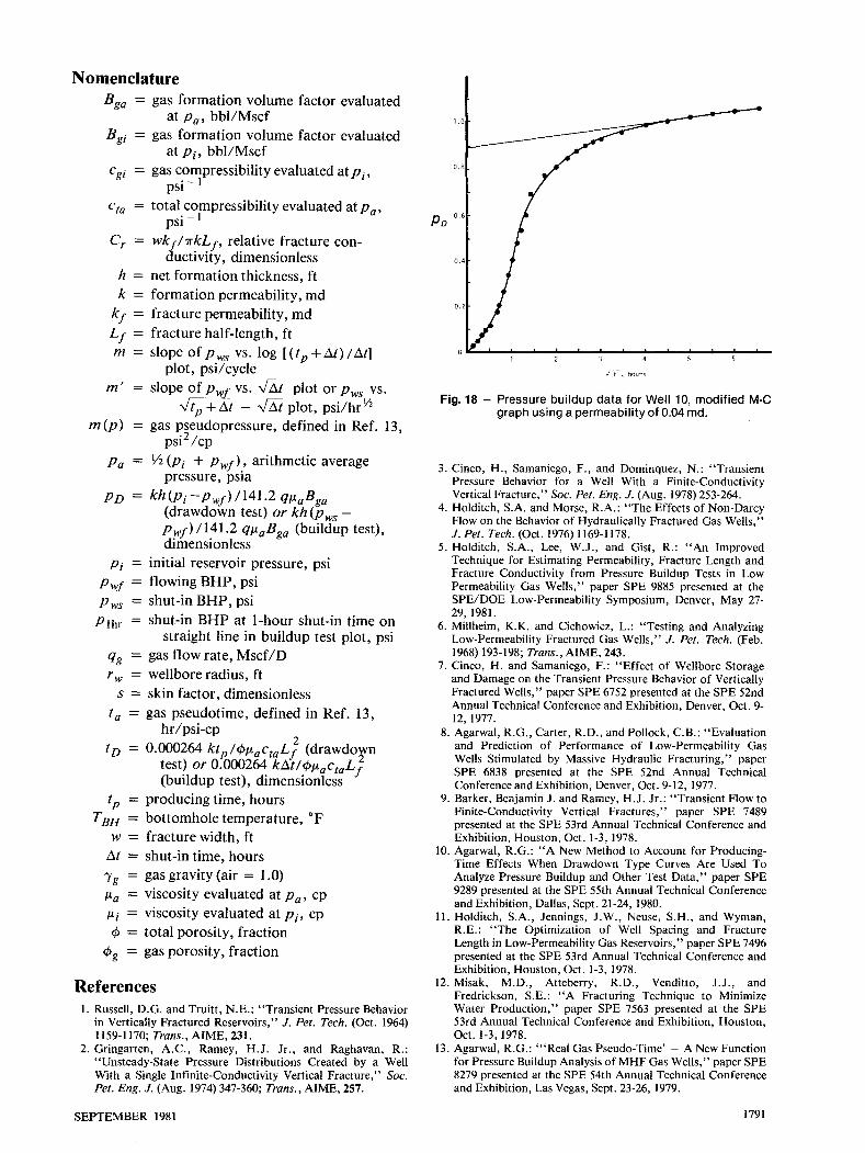
In the field data we have analyzed during the past few years, fracture conductivity normally has not been a problem. In reservoirs with permeabilities of 0.001 to 0.05 md and with fracture lengths of 500 to 1,500 ft, crushed sand usually will provide sufficient con­ductivity to drain a reservoir adequately. In some cases, however, crushing and/or embedment can present problems. Well 10 is a well with a low dimensionless conductivity. The pressure buildup data for Well 10 are presented in Table 9 and in Figs. 16,17, and 18.

Well 10 was perforated, acidized, and produced at a rate of 100 McflD at 600 psi flowing tubing pressure. A prefracture buildup survey indicated that

1787

1788

. 05

. 01

10

Fig. 13 - Pressure buildup data for Well 12, 10g·log graph.

A o A

1000

o FIELD DATA

I:;. HISTORY MATCH

o

100

(t+.t)/.t

10

Fig. 14 - Pressure buildup data for Well 12, Horner graph with results from history match .

, • • ••

• • •

• •

10

I"T""", hours

11 14 16 18 10

Fig. 15 - Pressure buildup data for Well 12, modified M·e graph using a permeability of 0.001 md.

JOURNAL OF PETROLEUM TECHNOLOGY

the in-situ permeability was about 0.02 md with a small negative skin. After the fracture treatment, the well produced about 1,300 McflD at 2,200 psi flowing tubing pressure. This response is a definite indication that the fracture treatment successfully stimulated the formation.

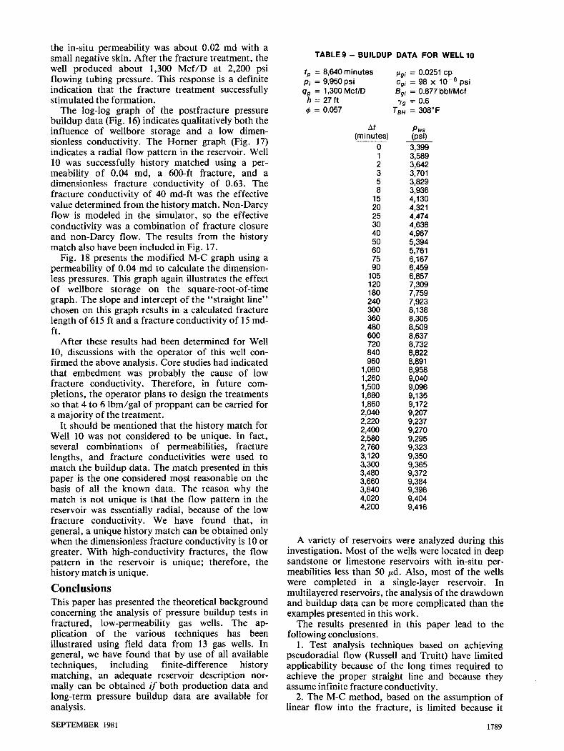
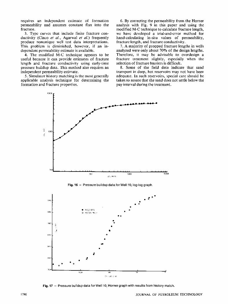
The log-log graph of the postfracture pressure buildup data (Fig. 16) indicates qualitatively both the influence of well bore storage and a low dimen­sionless conductivity. The Horner graph (Fig. 17) indicates a radial flow pattern in the reservoir. Well 10 was successfully history matched using a per­meability of 0.04 md, a 600-ft fracture, and a dimensionless fracture conductivity of 0.63. The fracture conductivity of 40 md-ft was the effective value determined from the history match. Non-Darcy flow is modeled in the simulator, so the effective conductivity was a combination of fracture closure and non-Darcy flow. The results from the history match also have been included in Fig. 17.

Fig. 18 presents the modified M-C graph using a permeability of 0.04 md to calculate the dimension­less pressures. This graph again illustrates the effect of well bore storage on the square-root-of-time graph. The slope and intercept of the "straight line" chosen on this graph results in a calculated fracture length of 615 ft and a fracture conductivity of 15 md­ft.

After these results had been determined for Well 10, discussions with the operator of this well con­firmed the above analysis. Core studies had indicated that embedment was probably the cause of low fracture conductivity. Therefore, in future com­pletions, the operator plans to design the treatments so that 4 to 6 Ibm/gal of proppant can be carried for a majority of the treatment.

It should be mentioned that the history match for Well 10 was not considered to be unique. In fact, several combinations of permeabilities, fracture lengths, and fracture conductivities were used to match the buildup data. The match presented in this paper is the one considered most reasonable on the basis of all the known data. The reason why the match is not unique is that the flow pattern in the reservoir was essentially radial, because of the low fracture conductivity. We have found that, in general, a unique history match can be obtained only when the dimensionless fracture conductivity is 10 or greater. With high-conductivity fractures, the flow pattern in the reservoir is unique; therefore, the history match is unique.

Conclusions This paper has presented the theoretical background concerning the analysis of pressure buildup tests in fractured, low-permeability gas wells. The ap­plication of the various techniques has been illustrated using field data from 13 gas wells. In general, we have found that by use of all available techniques, including finite-difference history matching, an adequate reservoir description nor­mally can be obtained if both production data and long-term pressure buildup data are available for analysis.

SEPTEMBER 1981

TABLE 9 - BUILDUP DATA FOR WELL 10

tp = 8,640 minutes Pi = 9,950 psi qg = 1,300 McttO

h = 27ft <!> = 0.057

t:.t (minutes)

o 1 2 3 5 8

15 20 25 30 40 50 60 75 90

105 120 180 240 300 360 480 600 720 840 960

1,080 1,260 1,500 1,680 1,860 2,040 2,220 2,400 2,580 2,760 3,120 3,300 3,480 3,660 3,840 4,020 4,200

P-gi = 0.0251 cp Cgi = 98 X 10- 6 psi Bgi = 0.677 bbltMct 'Yg = 0.6

TBH = 308°F

Pws

~ 3,399 3,589 3,642 3,701 3,829 3,936 4,130 4,321 4,474 4,638 4,967 5,394 5,761 6,167 6,459 6,857 7,309 7,759 7,923 8,138 8,306 8,509 8,637 8,732 8,822 8,891 8,958 9,040 9,096 9,135 9,172 9,207 9,237 9,270 9,295 9,323 9,350 9,365 9,372 9,384 9,396 9,404 9,416

A variety of reservoirs were analyzed during this investigation. Most of the wells were located in deep sandstone or limestone reservoirs with in-situ per­meabilities less than 50 ltd. Also, most of the wells were completed in a single-layer reservoir. In multilayered reservoirs, the analysis of the drawdown and buildup data can be more complicated than the examples presented in this work.

The results presented in this paper lead to the following conclusions.

1. Test analysis techniques based on achieving pseudoradial flow (Russell and Truitt) have limited applicability because of the long times required to achieve the proper straight line and because they assume infinite fracture conductivity.

2. The M-C method, based on the assumption of linear flow into the fracture, is limited because it

1789

requires an independent estimate of formation permeability and assumes constant flux into the fracture.

3. Type curves that include finite fracture con­ductivity (Cinco et at., Agarwal et at.) frequently produce non unique well test data interpretations. This problem is diminished, however, if an in­dependent permeability estimate is available.

4. The modified M-C technique appears to be useful because it can provide estimates of fracture length and fracture conductivity using early-time pressure buildup data. This method also requires an independent permeability estimate.

5. Simulator history matching is the most generally applicable analysis technique for determining the formation and fracture properties.

10000

6. By correcting the permeability from the Horner analysis with Fig. 9 in this paper and using the modified M-C technique to calculate fracture length, we have developed a trial-and-error method for hand-calculating in-situ values of permeability, fracture length, and fracture conductivity.

7. A majority of propped fracture lengths in wells analyzed were only about 70070 of the design lengths. Therefore, it may be advisable to overdesign a fracture treatment slightly, especially when the selection of fracture barriers is difficult.

8. Some of the field data indicate that sand transport in deep, hot reservoirs may not have been adequate. In such reservoirs, special care should be taken to assure that the sand does not settle below the pay interval during the treatment.

100"-_ ...... _ ................................. __ ............. _""-' ....... ...&..I...I..L __ .... _ ................... 1..I. ..... 10000

1790

9000

8000

7000 Q

,

6000

5000

4000

• • 0

3000

100 1000 ~t. mins

Fig. 16 - Pressure buildup data for Well 10, log-log graph .

• FIELD DATA

o HISTORY MATrH

•

• • o

1000

• o

•

100

• • o

(t tilt) 16t

• .0 •

o

• • 0

10

• • 0 • 0

Fig. 17 - Pressure buildup data for Well 10, Horner graph with results from history match.

JOURNAL OF PETROLEUM TECHNOLOGY

Nomenclature

Cr

h

k

k j L j m

m'

m(p)

P a

PD

Pi

Pwj

P ws

P1hr

qg

rw

s fa

ID

gas formation volume factor evaluated at Pa , bbl/Mscf

gas formation volume factor evaluated at Pi' bbl/Mscf

= gas compressibility evaluated atpi' psi -1

=

= = =

=

= = = =

total compressibility evaluated at P a' psi -1

W~I 7fkL j' relative fracture con-uctivity, dimensionless

net formation thickness, ft formation permeability, md fracture permeability, md fracture half-length, ft slope of P ws vs. log [(tp+.::lI)/.::lI]

plot, psi/cycle

SIOP~Of Pwf vs. -JfIi plot or P ws vs. I p +.::If - 51 plot, psi/hr Y2

gas pseudopressure, defined in Ref. 13, psi2/cp

V2 (Pi + Pwj).' arithmetic average pressure, pSIa

kh(Pi-Pwj) 1141.2 qJ1-aBga (draw down test) or kh (P ws -Pwj) 1141.2 qJ1-aBga (buildup test), dimensionless

initial reservoir pressure, psi flowing BHP, psi shut-in BHP, psi shut-in BHP at I-hour shut-in time on

straight line in buildup test plot, psi gas flow rate, MscflD wellbore radius, ft skin factor, dimensionless gas pseudotime, defined in Ref. 13,

hr/psi-cp 2

0.000264 ktpl¢J1-aCtaLj (drawdo~n test) or 0.000264 k.::lt/¢J1-aCtaLj (buildup test), dimensionless

I p = producing time, hours T BH = bottom hole temperature, OF

W = fracture width, ft t:.t = shut-in time, hours 'Y g = gas gravity (air = 1.0) J1-a = viscosity evaluated at P a , cp J1-i = viscosity evaluated at Pi' cp ¢ = total porosity, fraction

¢g = gas porosity, fraction

References 1. Russell, D.G. and Truitt, N.E.: "Transient Pressure Behavior

in Vertically Fractured Reservoirs," J. Pet. Tech. (Oct. 1964) 1159-1170; Trans., AIME, 231.

2. Gringarten, A.C., Ramey, H.J. Jr., and Raghavan, R.: "Unsteady-State Pressure Distributions Created by a Well With a Single Infinite-Conductivity Vertical Fracture," Soc. Pet. Eng. J. (Aug. 1974) 347-360; Trans., AIME, 257.

SEPTEMBER 1981

1.0

I-e, hours

Fig. 18 - Pressure buildup data for Well 10, modified M-e graph using a permeability of 0.04 md.

3. Cinco, H., Samaniego, F., and Dominquez, N.: "Transient Pressure Behavior for a Well With a Finite-Conductivity Vertical Fracture," Soc. Pet. Eng. J. (Aug. 1978) 253-264.

4. Holditch, S.A. and Morse, R.A.: "The Effects of Non-Darcy Flow on the Behavior of Hydraulically Fractured Gas Wells," J. Pet. Tech. (Oct. 1976) 1169-1178.

5. Holditch, S.A., Lee, W.J., and Gist, R.: "An Improved Technique for Estimating Permeability, Fracture Length and Fracture Conductivity from Pressure Buildup Tests in Low Permeability Gas Wells," paper SPE 9885 presented at the SPE/DOE Low-Permeability Symposium, Denver, May 27-29, 1981.

6. Millheim, K.K. and Cichowicz, L.: "Testing and Analyzing Low-Permeability Fractured Gas Wells," J. Pet. Tech. (Feb. 1968) 193-198; Trans., AIME, 243.

7. Cinco, H. and Samaniego, F.: "Effect of Well bore Storage and Damage on the Transient Pressure Behavior of Vertically Fractured Wells," paper SPE 6752 presented at the SPE 52nd Annual Technical Conference and Exhibition, Denver, Oct. 9-12, 1977.

8. Agarwal, R.G., Carter, R.D., and Pollock, C.B.: "Evaluation and Prediction of Performance of Low-Permeability Gas Wells Stimulated by Massive Hydraulic Fracturing," paper SPE 6838 presented at the SPE 52nd Annual Technical Conference and Exhibition, Denver, Oct. 9-12, 1977.

9. Barker, Benjamin J. and Ramey, H.J. Jr.: "Transient Flow to Finite-Conductivity Vertical Fractures," paper SPE 7489 presented at the SPE 53rd Annual Technical Conference and Exhibition, Houston, Oct. 1-3, 1978.

10. Agarwal, R.G.: "A New Method to Account for Producing­Time Effects When Drawdown Type Curves Are Used To Analyze Pressure Buildup and Other Test Data," paper SPE 9289 presented at the SPE 55th Annual Technical Conference and Exhibition, Dallas, Sept. 21-24,1980.

11. Holditch, S.A., Jennings, J.W., Neuse, S.H., and Wyman, R.E.: "The Optimization of Well Spacing and Fracture Length in Low-Permeability Gas Reservoirs," paper SPE 7496 presented at the SPE 53rd Annual Technical Conference and Exhibition, Houston, Oct. 1-3, 1978.

12. Misak, M.D., Atteberry, R.D., Venditto, J.J., and Fredrickson, S.E.: "A Fracturing Technique to Minimize Water Production," paper SPE 7563 presented at the SPE 53rd Annual Technical Conference and Exhibition, Houston, Oct. 1-3, 1978.

13. Agarwal, R.G.: '''Real Gas Pseudo-Time' - A New Function for Pressure Buildup Analysis of MHF Gas Wells," paper SPE 8279 presented at the SPE 54th Annual Technical Conference and Exhibition, Las Vegas, Sept. 23-26,1979.

1791

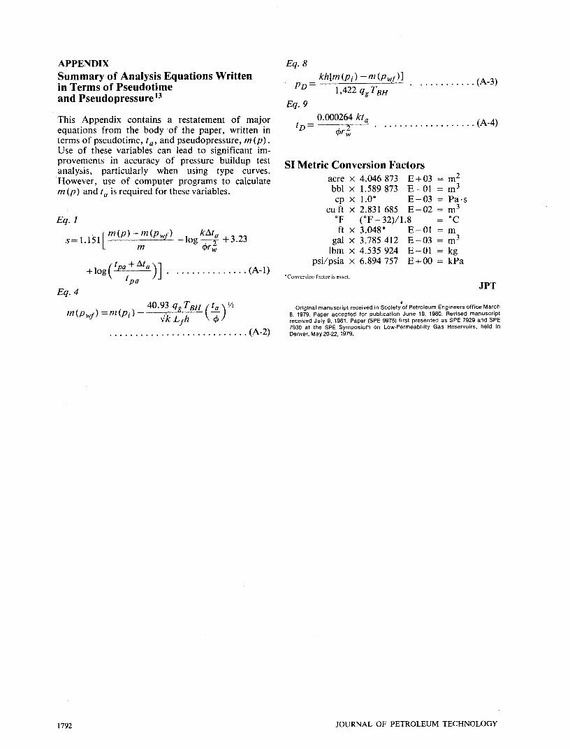
APPENDIX Summary of Analysis Equations Written in Terms of Pseudotime and Pseudopressure 13

This Appendix contains a restatement of major equations from the body 'of the paper, written in terms of pseudotime, I a' and pseudopressure, m (p) . Use of these variables can lead to significant im­provements in accuracy of pressure buildup test analysis, particularly when using type curves. However, use of computer programs to calculate m(p) and ta is required for these variables.

Eq.l

s= 1.151 [m(p) -mm(Pwj ) -log kAla +3.23 ¢r;

(tpa+Ala)] + log ............... (A-I)

t pa Eq.4

40.93 qg TBH (!.E.-) \12 m(pwj) =m(Pi) VI<: Ljh ¢

........................... (A-2)

1792

Eq.B

Eq.9

0.000264 kta tD = 2 ......•.....•.....• (A-4)

¢rw

Sf Metric Conversion Factors acre x 4.046873 E+03 = m2

bbl x 1.589873 E-Ol = m3

cp X 1.0* E-03 = Pa·s cu ft x 2.831 685 E-02 = m3

OF CF - 32)/1.8 °C ft x 3.048* E-Ol m

gal x 3.785412 E-03 m3

Ibm x 4.535924 E-Ol kg psilpsia x 6.894757 E+OO kPa

·Conversion factor is exact.

JPT

. Original manuscript received in Society of Petroleum Engineers office March

8, 1979. Paper accepted for publication June 19, 1980. Revised manuscript received July 9,1981. Paper (SPE 9975) first presented as SPE 7929 and SPE 7930 at the SPE Symposium on Low·Permeability Gas Reservoirs, held in Denver, May 20·22,1979.

JOURNAL OF PETROLEUM TECHNOLOGY