FRACTIONAL MODEL ON THE DYNAMICS OFCHICKEN POX WITH VACCINATION

1 Aguegboh,Nnaemeka S, 2Uko Ofe,3Netochukwu E. Onyiaji,4Ugwu O. Lovelyn1Department of Mathematics, Veritas University, Abuja 2Department of Pure and

Applied Physics, Veritas University, Abuja 3Department of Mathematics, University of

Nigeria, Nsukka 4Department of Microbiology,Veritas University, Abuja1aguegboh@veritas.edu.ng

2ukoo@veritas.edu.ng3onyiajineto@gmail.com4ugwuo@veritas.edu.ng

Abstract

In this paper, we proposed a fractional SVIR order model to study the transmission dynamics of Chick-

enpox. We showed the existence of the equilibrium states. The basic reproduction number of the model

was evaluated in terms of parameters in the model using the next generation matrix approach. We

provided the conditions for the stability of the disease-free and the endemic equilibrium points. Also a

detailed stability analysis of the model was carried out. Also, numerical simulations of the model were

carried out using Adams-type predictor-corrector method and the paper provided a theoretical basis to

control the spread of Chickenpox.

Keywords: Fractional calculus, Chickenpox, Numerical solution, Predictor-corrector method

1 Introduction

Chicken pox also known as Varicella is a viral disease caused by an infectious disease virus known as

Varicella-Zoster virus. It is a contagious viral disease that predominantly affects children. It is often a

mild illness, characterized by an itchy rash on the face, scalp and trunk with pink spots and tiny fluid-

filled blisters that dries and become scabs four to five days later. Serious complications, although rare

can occur mainly in infants, adolescents, adults and persons with a weakened immune system. Those

complications include bacterial infections of skin blisters, pneumonia and encephalitis (inflammation of

the brain). In temperate climates, such as the Northeast, chicken pox occurs most frequently in the late

winter and early spring.[1] Chicken pox is a common childhood illness with 90 of the cases occurring

in children younger than ten (10) years of age. The risk of complications depends on age and level of

immunity. Chicken pox is characterized by peculiar symptoms such as slight fever, fatigue, difficulty

in breathing, malaise, irritability, after some days, symptoms like itchy rashes may appear. The rashes

starts with crops of small red bumps on the stomach or back and spread to the face, limbs and other

1

parts of the body except palms and foot. The itchy rashes then develop into numbers between 250 and

500 which becomes blisters and last for a maximum of 5 to 7 days.[2]

Berreta and Capasso [3] studied rubella epidemiology in South East England. The disease was char-

acterized by age-dependent changes in the pattern of virus transmission. The rate of infection was

low in children than in adults. Immunization against people raised levels of immunity in both children

and adults. On average, antibody concentrations recorded a reduction with age and low in vaccinated

females than in unvaccinated males.Kermack and McKendrick citefour studied epidemics of measles

in United Kingdom. In their study the dynamics of the disease depended on infections rate, the re-

moval rate and relative removal rate. Their work observed that the disease threshold occurs when

basic reproductive number equals to one. Li and Zou [5] applied a generalization of the Kemack and

McKendrik [4] model to a patchy environment for a disease with latency. Their work assumed that the

infectious disease had a fixed latent period in a population. In a paper Furguson et al [1], reviewed

and discussed different hypotheses of how this re-emergence of virus comes about. From these hypothe-

ses, and epidemiological data describing the initial transmission of the virus, a mathematical model of

primary disease (varicella) and reactivated disease (zoster) in developed countries was derived. Most

researchers in the past hardly discussed transmission dynamics of Chickenpox with vaccination by ap-

plying fractional calculus. Inspired by this, in the present work we considered the fractional order SVIR

model by using a system of fractional order differential equation in the sense of Caputo, for prevention

of Chickenpox with vaccination.. By applying fractional calculus, we gave a detailed analysis on the

stability of the disease free and endemic equilibrium points. Also numerical simulation was carried out

to illustrate the obtained results.

Mathematical modeling of infectious diseases using integer order system of differential equations has

gained a lot of attention over the past years[6]. However, epidemiological models and other models in

science and engineering have successfully been formulated and analyzed using fractional derivatives and

integrals[7, 8]. Fractional derivatives are nonlocal as opposed to the local behavior of integer derivatives.

This implies that the next state of a fractional system does not only depend on its current state but

also upon all of its historical states [15].

2 Fractional Order Calculus

Fractional order models have been the focus of many studies due to their frequent appearance in various

applications in several scientific fields. We first give the definition of fractional-order integration and

fractional order differentiation. For the concept of fractional derivative, we will consider Caputo’s

definition. It has an advantage of dealing properly with initial value problem.

2.1 Definition of terms

Definition 1. The Caputo Fractional derivative of order α of a function f : <+ → < is given by

Dαt f(t) =

1

Γ(α− n)

∫ t

α

f (n)(τ)dτ

(t− τ)α+1−n (n− 1 < α ≤ n) (1)

2

Definition 2. The formular for the Laplace transform of the Caputo derivative is given by

∫ ∞0

e−ptDαt f(t)dt = pαF (p)−

n−1∑k=0

pα−k−1f (k)(0), (n− 1 < α ≤ n) (2)

Definition 3. The Fractional integral of order α of a function f : <+ → < is given by

Jα(f(x)) =1

Γ(α)

∫ x

0

(x− t)α−1f(t)dt, α > 0, x > 0 (3)

Definition 4. The fractional integral of the Caputo Fractional derivative of order α of a function

f : <+ → < is given by

JαDαf(t) = f(t)−n−1∑k=0

f (k)(0)tk

k!, t > 0 (4)

Definition 5. A two-parameter function of the Mittag-Leffler type is defined by the series expansion

Eα,β(z) =∞∑k=0

zk

Γ(αk + β), (α, β > 0) (5)

3 Model Formulation

The SVIR model is based on the following assumptions:

1. Let S, I, V, R denote the densities (or fractions) of Susceptible class, infected class, vaccinated class

and recovered/removed individuals respectively.

2. We assumed that the susceptible individuals are recruited at an influx rate of Λ.

3. We assumed that µ be the natural death rate of the population.

4. Let β be the transmission rate of disease when susceptible individuals contact with infected individ-

uals.

5. Let γ be the recovery rate of infected individuals.

6. The recovered individuals are assumed to have immunity (so called natural immunity) against the

disease.

7. Let θ be the rate at which susceptible individuals are removed into the vaccinated class.

8. Let γ1 be the average rate for the vaccinated individuals obtaining immunity and move into the

recovered population.

9. We assumed that before obtaining immunity the vaccines still have the possibility of infection with

a disease transmission rate β1 while contacting the infected individuals.

Now, putting these assumptions together, we have the model flow diagram and thus the model equations

for the transmission of Chickenpox.

The schematic diagram of the disease on which we base our model is as follow:

3

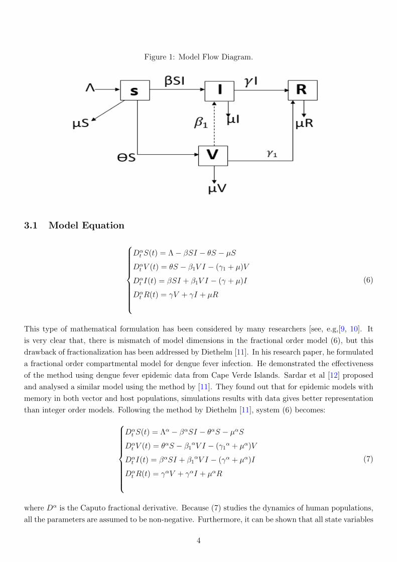
Figure 1: Model Flow Diagram.

3.1 Model Equation

Dαt S(t) = Λ− βSI − θS − µS

Dαt V (t) = θS − β1V I − (γ1 + µ)V

Dαt I(t) = βSI + β1V I − (γ + µ)I

Dαt R(t) = γV + γI + µR

(6)

This type of mathematical formulation has been considered by many researchers [see, e.g,[9, 10]. It

is very clear that, there is mismatch of model dimensions in the fractional order model (6), but this

drawback of fractionalization has been addressed by Diethelm [11]. In his research paper, he formulated

a fractional order compartmental model for dengue fever infection. He demonstrated the effectiveness

of the method using dengue fever epidemic data from Cape Verde Islands. Sardar et al [12] proposed

and analysed a similar model using the method by [11]. They found out that for epidemic models with

memory in both vector and host populations, simulations results with data gives better representation

than integer order models. Following the method by Diethelm [11], system (6) becomes:

Dαt S(t) = Λα − βαSI − θαS − µαS

Dαt V (t) = θαS − β1

αV I − (γ1α + µα)V

Dαt I(t) = βαSI + β1

αV I − (γα + µα)I

Dαt R(t) = γαV + γαI + µαR

(7)

where Dα is the Caputo fractional derivative. Because (7) studies the dynamics of human populations,

all the parameters are assumed to be non-negative. Furthermore, it can be shown that all state variables

4

of the model are non-negative for all time t≥0.

3.2 Invariant Region

Lemma 4. The closed set Ω = (S, V, I, R) ∈ R4+ : S + I + R + A ≤ Λ

µ is positively invariant with

respect to model (7)

Proof

The fractional derivative of the total human population, obtained by adding all the human equations

of model (7), is given by

DαN(t) = Λ− µN(t) (8)

Taking the Laplace transform of (8) gives:

SαN(s)− Sα−1N(0) =Λ

S− µN(s)

⇒ N(s) =Λ

S(Sα + µ)+

Sα−1

sα + µN(0) (9)

Taking the inverse Laplace transform of (9), we have:

N(t) = N(0)Eα,1(−µtα) + ΛtαEα,α+1(−µtα) (10)

where Eα,β is the Mittag-Leffler function. But the fact that the Mittag-Leffler functions has an asymp-

totic behavior[13, 14], it follows that:

Eα,1N(t) =∞∑k=0

NK(t)

Γ(αk + 1), α > 0 (11)

Eα,α+1N(t) =∞∑k=0

NK(t)

Γ(αk + α + 1), α > 0 (12)

Expanding (11), we have

Eα,1N(t) =1

Γ1+

N(t)

Γ(α + 1)+

N2(t)

Γ(2α + 1)+ ...

Expanding (12), we have

Eα,α+1N(t) =1

Γ(α + 1)+

N(t)

Γ(2α + 1)+

N2(t)

Γ(3α + 1)+ ...

Since Mittag-Leffler function has an asymptotic property, we have

N(t) = 1 +O(N)

5

Taking limit as k−→∞, we have

N(t) ≈ 1

Then, it is clear that Ω is a positive invariant set.Therefore, all solutions of the model with initial

conditions in Ω remain in Ω for all t > 0. Then , Ω = N(t) > 0 implies that it is feasible with respect

to model (7).

5 Model Analysis

5.1 The Basic Reproduction Number, R0

To calculate the reproduction number (R0), we use the Next Generation Matrix. It is comprised of two

parts: F and V −1,

∴ R0 = ρ(FV −1)

Where

F =∣∣∣∂fix(0)∂xj

∣∣∣ , V =∣∣∣∂vix(0)∂xj

∣∣∣ρ = spectral value ( highest eigenvalue)

On the estimation,We used the following disease compartments:

Dαt V (t) = θαS − β1

αV I − (γ1α + µα)V

Dαt I(t) = βαSI + β1

αV I − (γα + µα)I

(13)

Define

Fi =

−β1αV I

βαSI + β1αV I

−Vi =

(θαS − (γ1

α + µα)V

−(γα + µα)I

)

FV −1 =

(0 0

0 βαΛα

(θα+µα)(γα+µα)

)Hence,

R0 =βαΛα

(θα + µα)(γα + µα)(14)

6

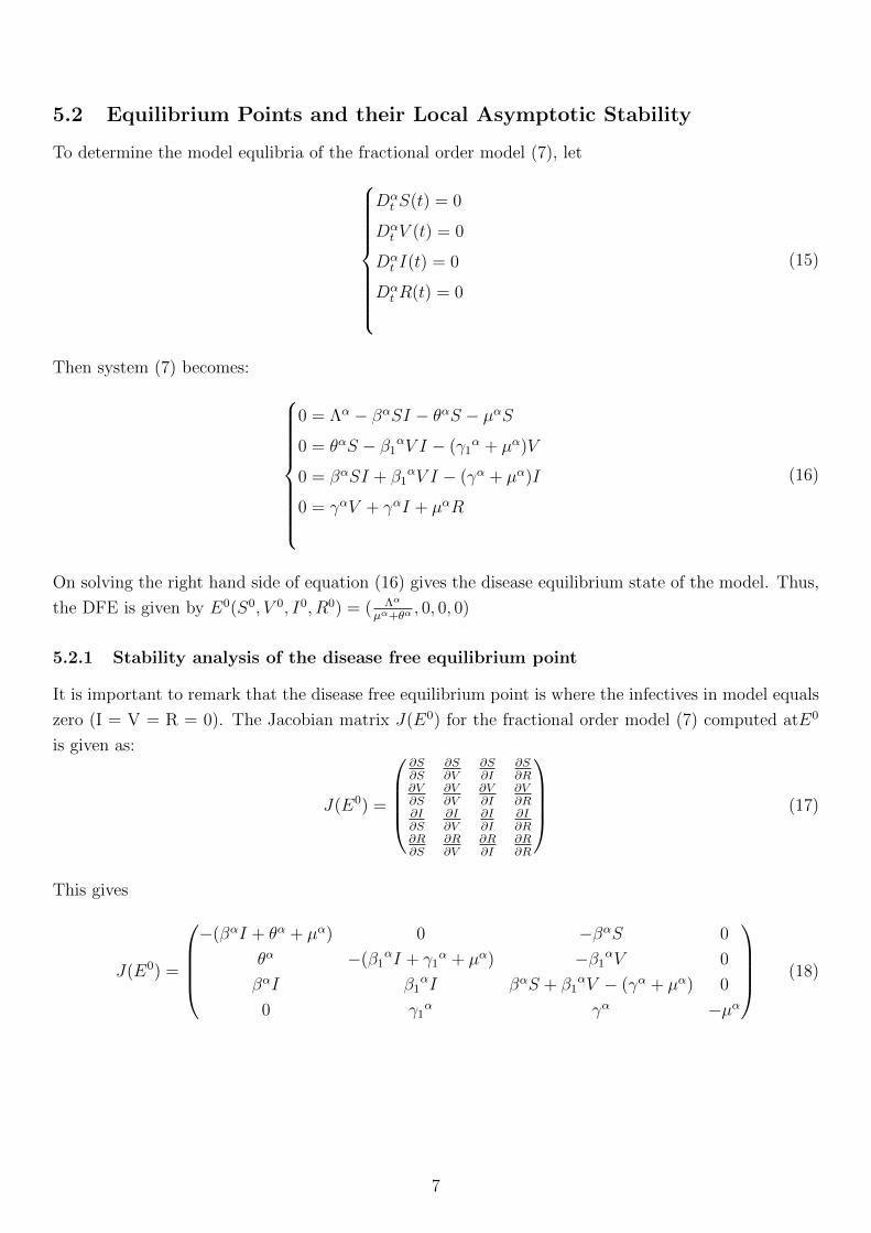
5.2 Equilibrium Points and their Local Asymptotic Stability

To determine the model equlibria of the fractional order model (7), let

Dαt S(t) = 0

Dαt V (t) = 0

Dαt I(t) = 0

Dαt R(t) = 0

(15)

Then system (7) becomes:

0 = Λα − βαSI − θαS − µαS

0 = θαS − β1αV I − (γ1

α + µα)V

0 = βαSI + β1αV I − (γα + µα)I

0 = γαV + γαI + µαR

(16)

On solving the right hand side of equation (16) gives the disease equilibrium state of the model. Thus,

the DFE is given by E0(S0, V 0, I0, R0) = ( Λα

µα+θα, 0, 0, 0)

5.2.1 Stability analysis of the disease free equilibrium point

It is important to remark that the disease free equilibrium point is where the infectives in model equals

zero (I = V = R = 0). The Jacobian matrix J(E0) for the fractional order model (7) computed atE0

is given as:

J(E0) =

∂S∂S

∂S∂V

∂S∂I

∂S∂R

∂V∂S

∂V∂V

∂V∂I

∂V∂R

∂I∂S

∂I∂V

∂I∂I

∂I∂R

∂R∂S

∂R∂V

∂R∂I

∂R∂R

(17)

This gives

J(E0) =

−(βαI + θα + µα) 0 −βαS 0

θα −(β1αI + γ1

α + µα) −β1αV 0

βαI β1αI βαS + β1

αV − (γα + µα) 0

0 γ1α γα −µα

(18)

7

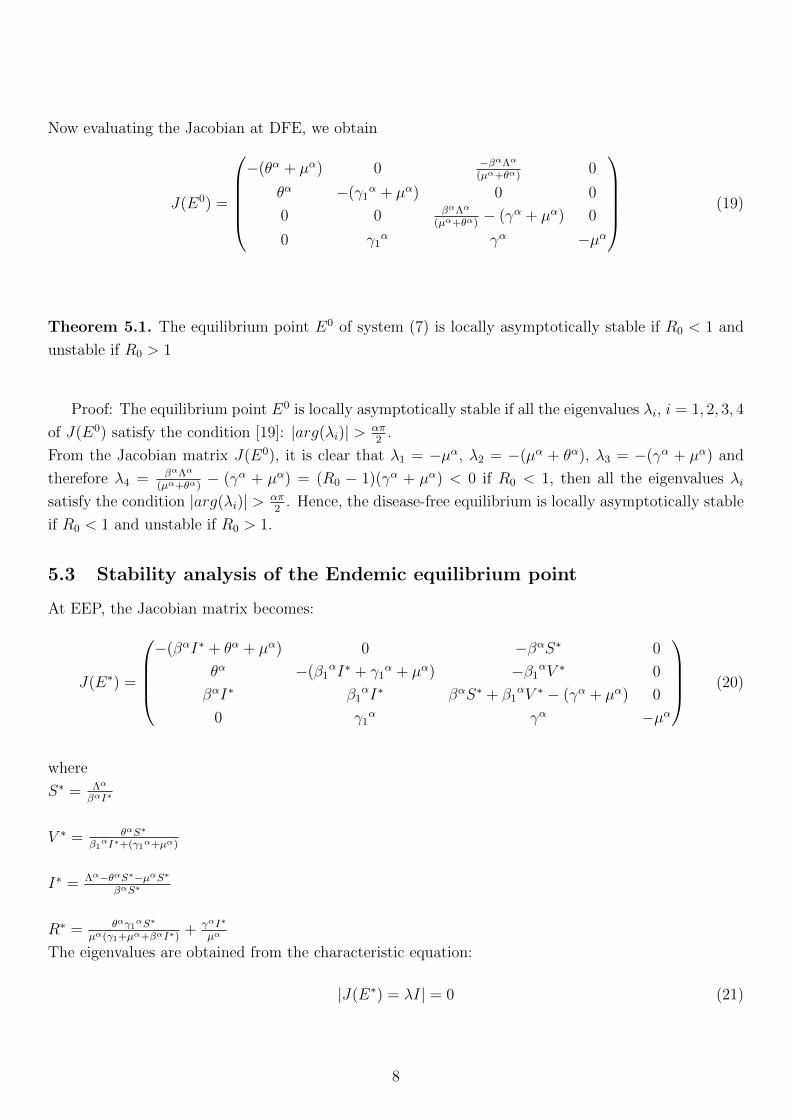
Now evaluating the Jacobian at DFE, we obtain

J(E0) =

−(θα + µα) 0 −βαΛα

(µα+θα)0

θα −(γ1α + µα) 0 0

0 0 βαΛα

(µα+θα)− (γα + µα) 0

0 γ1α γα −µα

(19)

Theorem 5.1. The equilibrium point E0 of system (7) is locally asymptotically stable if R0 < 1 and

unstable if R0 > 1

Proof: The equilibrium point E0 is locally asymptotically stable if all the eigenvalues λi, i = 1, 2, 3, 4

of J(E0) satisfy the condition [19]: |arg(λi)| > απ2

.

From the Jacobian matrix J(E0), it is clear that λ1 = −µα, λ2 = −(µα + θα), λ3 = −(γα + µα) and

therefore λ4 = βαΛα

(µα+θα)− (γα + µα) = (R0 − 1)(γα + µα) < 0 if R0 < 1, then all the eigenvalues λi

satisfy the condition |arg(λi)| > απ2

. Hence, the disease-free equilibrium is locally asymptotically stable

if R0 < 1 and unstable if R0 > 1.

5.3 Stability analysis of the Endemic equilibrium point

At EEP, the Jacobian matrix becomes:

J(E∗) =

−(βαI∗ + θα + µα) 0 −βαS∗ 0

θα −(β1αI∗ + γ1

α + µα) −β1αV ∗ 0

βαI∗ β1αI∗ βαS∗ + β1

αV ∗ − (γα + µα) 0

0 γ1α γα −µα

(20)

where

S∗ = Λα

βαI∗

V ∗ = θαS∗

β1αI∗+(γ1α+µα)

I∗ = Λα−θαS∗−µαS∗

βαS∗

R∗ = θαγ1αS∗

µα(γ1+µα+βαI∗)+ γαI∗

µα

The eigenvalues are obtained from the characteristic equation:

|J(E∗) = λI| = 0 (21)

8

Thus, −(βαI∗ + θα + µα) 0 −βαS∗ 0

θα −(β1αI∗ + γ1

α + µα) −β1αV ∗ 0

βαI∗ β1αI∗ βαS∗ + β1

αV ∗ − (γα + µα) 0

0 γ1α γα −µα

= 0 (22)

The characteristic equation J(E∗) is given as

(−µα − λ)(λ3 + a1λ2 + a2λ+ a3) = 0 (23)

Where

a1 =µα

S∗+θαS∗

V ∗> 0, a2 =

θαµα

V ∗+β1

2αV ∗I∗+β2αS∗I∗ > 0, a3 = θαβαβ1αS∗I∗+

θαβ2αS∗2I∗

V ∗+µαβ1

2αV ∗I∗

S∗> 0.

Since a1a2 > a3, by Routh-Hurwitz criterion [6],the eigenvalues have negative real parts. Therefore,

the endemic equilibrium point is stable.

6 Numerical Simulation

In this section, the predictor corrector method is applied to get the numerical solutions of system (7)

[12]. We will propose two cases for the model (7) with various values of parameters. In the first case,

λ = 1 ,β = 10 , µ = 1 , γ = 4 , β1 = 2 , θ = 10 , γ1 = 8 [13] and with initial conditions: S (0) = 500

, E (0) = 5 , I (0) = 20 , R(0) = 10 (Estimated). In this case, R0 = 0.2 < 1, then the disease free

equilibrium is locally stable and the disease dies out. In the second case,λ = 1 ,β = 20 , µ = 1 , γ = 1

,β1 = 2 , θ = 5 , γ1 = 8 with same initial conditions, then R = 1.67 > 1 which implies that the disease

still persists and the endemic equilibrium is globally stable.

9

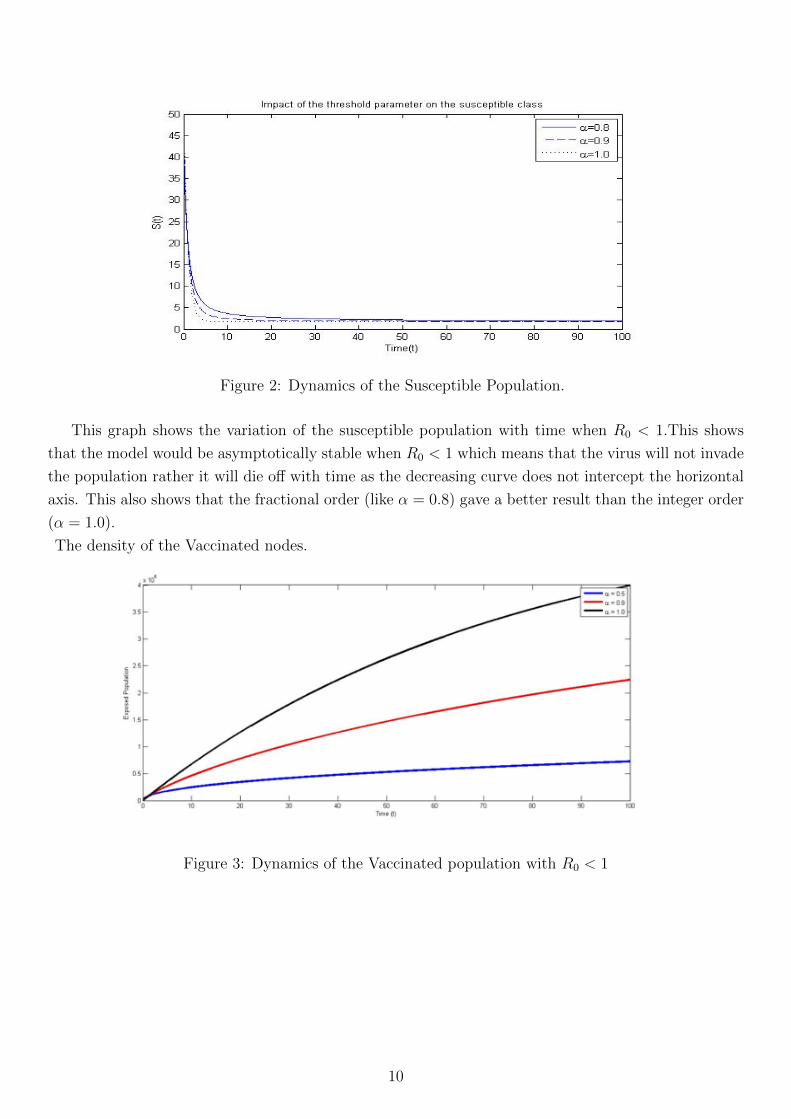
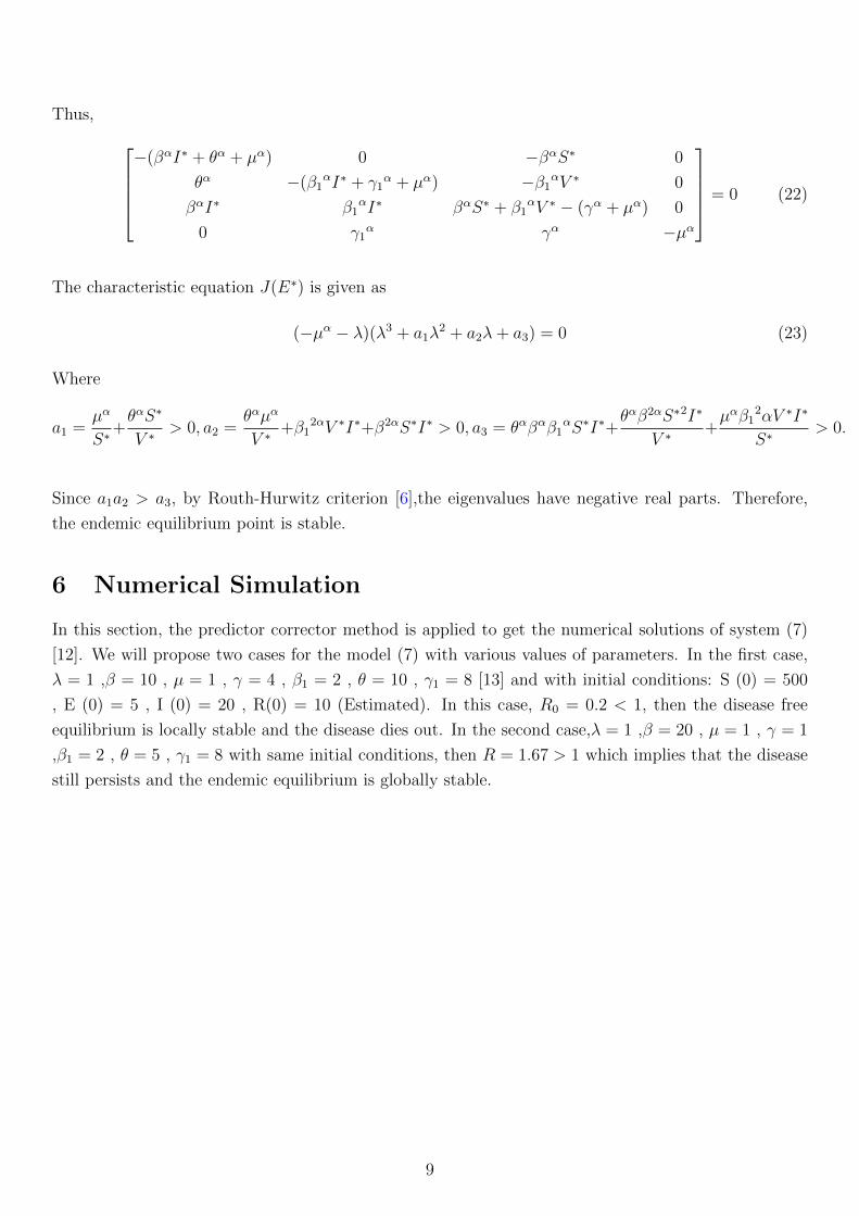
Figure 2: Dynamics of the Susceptible Population.

This graph shows the variation of the susceptible population with time when R0 < 1.This shows

that the model would be asymptotically stable when R0 < 1 which means that the virus will not invade

the population rather it will die off with time as the decreasing curve does not intercept the horizontal

axis. This also shows that the fractional order (like α = 0.8) gave a better result than the integer order

(α = 1.0).

The density of the Vaccinated nodes.

Figure 3: Dynamics of the Vaccinated population with R0 < 1

10

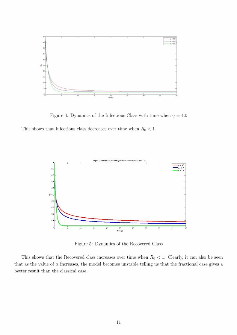
Figure 4: Dynamics of the Infectious Class with time when γ = 4.0

This shows that Infectious class decreases over time when R0 < 1.

Figure 5: Dynamics of the Recovered Class

This shows that the Recovered class increases over time when R0 < 1. Clearly, it can also be seen

that as the value of α increases, the model becomes unstable telling us that the fractional case gives a

better result than the classical case.

11

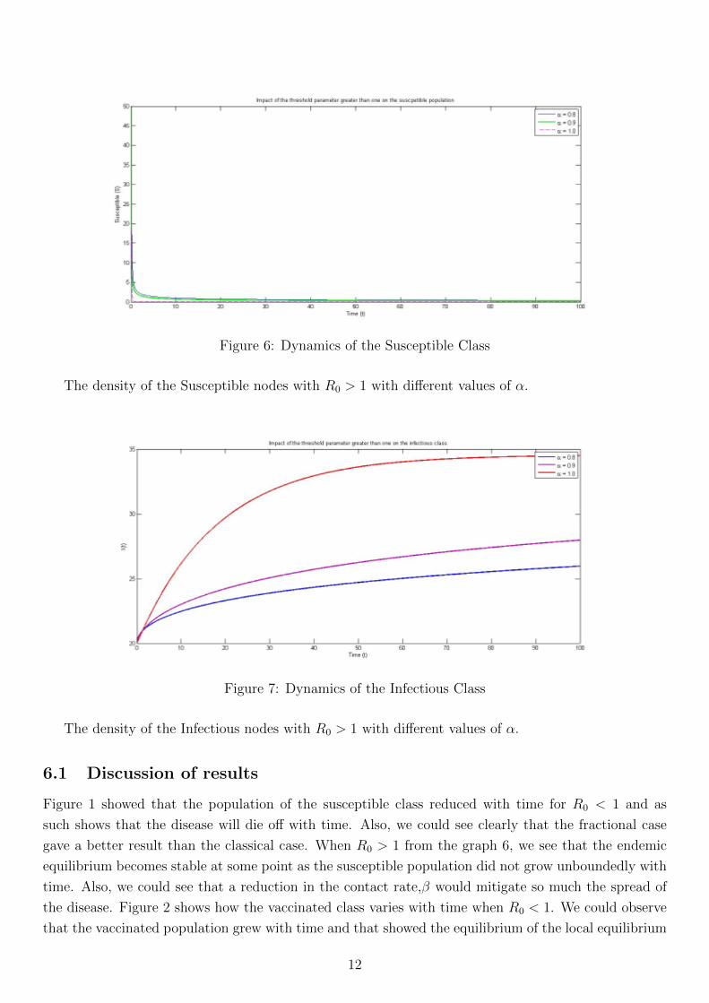
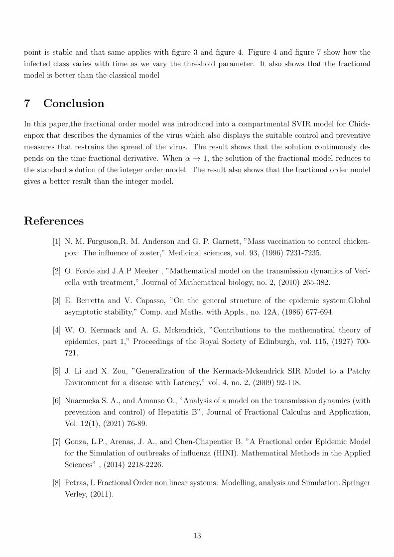
Figure 6: Dynamics of the Susceptible Class

The density of the Susceptible nodes with R0 > 1 with different values of α.

Figure 7: Dynamics of the Infectious Class

The density of the Infectious nodes with R0 > 1 with different values of α.

6.1 Discussion of results

Figure 1 showed that the population of the susceptible class reduced with time for R0 < 1 and as

such shows that the disease will die off with time. Also, we could see clearly that the fractional case

gave a better result than the classical case. When R0 > 1 from the graph 6, we see that the endemic

equilibrium becomes stable at some point as the susceptible population did not grow unboundedly with

time. Also, we could see that a reduction in the contact rate,β would mitigate so much the spread of

the disease. Figure 2 shows how the vaccinated class varies with time when R0 < 1. We could observe

that the vaccinated population grew with time and that showed the equilibrium of the local equilibrium

12

point is stable and that same applies with figure 3 and figure 4. Figure 4 and figure 7 show how the

infected class varies with time as we vary the threshold parameter. It also shows that the fractional

model is better than the classical model

7 Conclusion

In this paper,the fractional order model was introduced into a compartmental SVIR model for Chick-

enpox that describes the dynamics of the virus which also displays the suitable control and preventive

measures that restrains the spread of the virus. The result shows that the solution continuously de-

pends on the time-fractional derivative. When α → 1, the solution of the fractional model reduces to

the standard solution of the integer order model. The result also shows that the fractional order model

gives a better result than the integer model.

References

[1] N. M. Furguson,R. M. Anderson and G. P. Garnett, ”Mass vaccination to control chicken-

pox: The influence of zoster,” Medicinal sciences, vol. 93, (1996) 7231-7235.

[2] O. Forde and J.A.P Meeker , ”Mathematical model on the transmission dynamics of Veri-

cella with treatment,” Journal of Mathematical biology, no. 2, (2010) 265-382.

[3] E. Berretta and V. Capasso, ”On the general structure of the epidemic system:Global

asymptotic stability,” Comp. and Maths. with Appls., no. 12A, (1986) 677-694.

[4] W. O. Kermack and A. G. Mckendrick, ”Contributions to the mathematical theory of

epidemics, part 1,” Proceedings of the Royal Society of Edinburgh, vol. 115, (1927) 700-

721.

[5] J. Li and X. Zou, ”Generalization of the Kermack-Mckendrick SIR Model to a Patchy

Environment for a disease with Latency,” vol. 4, no. 2, (2009) 92-118.

[6] Nnaemeka S. A., and Amanso O., ”Analysis of a model on the transmission dynamics (with

prevention and control) of Hepatitis B”, Journal of Fractional Calculus and Application,

Vol. 12(1), (2021) 76-89.

[7] Gonza, L.P., Arenas, J. A., and Chen-Chapentier B. ”A Fractional order Epidemic Model

for the Simulation of outbreaks of influenza (HINI). Mathematical Methods in the Applied

Sciences” , (2014) 2218-2226.

[8] Petras, I. Fractional Order non linear systems: Modelling, analysis and Simulation. Springer

Verley, (2011).

13

[9] E. Ahmed, A. M. A. El-Sayed and H. A. A. El-Saka, ”Equilibrium points,stability and

numerical solutions of fractional-order predator-prey and rabies models,” J. Math. Anal.

Appl., no. 325, (2007) 542-553.

[10] I. Area, H. Batarfi, J. Losada, JJ Nieto, M. Shammakh and A. Torres, ”On a fractional

order ebola epidemic model,” Advances in Difference Equations, (2015) 278.

[11] K. Diethelm, ”A fractional calculus based model for the simulation of an outbreak of dengue

fever,” Nonlinear Dynamics, vol. 71, no. 4, (2011) 613-619.

[12] T. Sardar, S. Rana, S. Bhattacharya, K. Al-Khaled and J. Chattopadhyay, ”A generic

model for a single strain mosquito-transmitted disease with memory on the host and the

vector,” Mathematical Biosciences, no. 263, (2015) 18-36.

[13] I. Podlubny, Fractional Differential Equations, Academic Press, (1999).

[14] R. Gorenglo, J. Loutchko and Y. Luchko, ”Computation of the Mittag-Leffler function and

its derivative,” Fractional Calculus and Applied Analysis, vol. 5, no. 4, (2002) 491-518.

[15] Aguegboh, N.S., Nwokoye, N.R., Onyiaji, N.E., Amanso, O.R. and Oranugo, D.O. (2020) A

Fractional Order Model for the Transmission Dynamics of Measles with Vaccination. Open

Access Library Journal , 7: e6670. https://doi.org/10.4236/oalib 1106670.

14