Mech Time-Depend Mater (2015) 19:209–228DOI 10.1007/s11043-015-9260-1

Fractional calculus model of articular cartilage basedon experimental stress-relaxation

P.A. Smyth1 · I. Green1

Received: 8 January 2014 / Accepted: 24 February 2015 / Published online: 10 March 2015© Springer Science+Business Media Dordrecht 2015

Abstract Articular cartilage is a unique substance that protects joints from damage andwear. Many decades of research have led to detailed biphasic and triphasic models for theintricate structure and behavior of cartilage. However, the models contain many assumptionson boundary conditions, permeability, viscosity, model size, loading, etc., that complicatethe description of cartilage. For impact studies or biomimetic applications, cartilage canbe studied phenomenologically to reduce modeling complexity. This work reports experi-mental results on the stress-relaxation of equine articular cartilage in unconfined loading.The response is described by a fractional calculus viscoelastic model, which gives storageand loss moduli as functions of frequency, rendering multiple advantages: (1) the fractionalcalculus model is robust, meaning that fewer constants are needed to accurately capture awide spectrum of viscoelastic behavior compared to other viscoelastic models (e.g., Pronyseries), (2) in the special case where the fractional derivative is 1/2, it is shown that thereis a straightforward time-domain representation, (3) the eigenvalue problem is simplified insubsequent dynamic studies, and (4) cartilage stress-relaxation can be described with as fewas three constants, giving an advantage for large-scale dynamic studies that account for jointmotion or impact. Moreover, the resulting storage and loss moduli can quantify healthy,damaged, or cultured cartilage, as well as artificial joints. The proposed characterization issuited for high-level analysis of multiphase materials, where the separate contribution ofeach phase is not desired. Potential uses of this analysis include biomimetic dampers andbearings, or artificial joints where the effective stiffness and damping are fundamental pa-rameters.

Keywords Articular cartilage · Fractional calculus · Unconfined compression ·Relaxation · Storage and loss modulus · Viscoelasticity

B P.A. Smythpasmyth4@gatech.edu

I. Greenitzhak.green@me.gatech.edu

1 School of Mechanical Engineering, Georgia Institute of Technology, Atlanta, GA 30332, USA

210 Mech Time-Depend Mater (2015) 19:209–228

NomenclatureCERF Complementary error viscoelastic modelE(t) Time-dependent relaxation modulusE(t) Time derivative of relaxation modulusE′(ω) Storage modulusE′′(ω) Loss modulusE∗(ω) Complex modulus, E′(ω) + iE′′(ω)

erfc Complementary error functioni Imaginary unitn Indexs Laplace variableα Fractional derivative orderε(t) Strainε(t) Strain rateη Spring-pot time constantΓ Gamma functionμ CERF model material constant, E/η

ω Frequency (rad/s)σ(t) Stress

1 Introduction

Articular cartilage facilitates motion in joints while providing compressive load support.The porous, biphasic (solid–fluid) structure of cartilage has been studied for many decades.This has led to advances in constitutive modeling, artificial joint replacements, and the char-acterization of osteoarthritis. Mechanical tests are performed to corroborate the prevailingbiphasic and triphasic (solid–fluid–ionic) models. A variety of experiments are used to testcartilage. In stress-relaxation experiments, cartilage displays elastic and dissipative mecha-nisms. These mechanisms are also central in viscoelastic materials, which are prevalent intraditional mechanical systems. Interesting applications for biomimetic materials, based oncartilage, arise from the study of biphasic materials. These include flexible mechanical bear-ings in rotordynamic systems (Grybos 1991; Friswell 2007) and improved porous bearingsin industrial applications (Elsharkawy and Nassar 1996).

A great deal of cartilage research has focused on the interactions of the collagen ma-trix and the lubricating synovial fluid that permeates the joint capsule (Charnley 1960;McCutchen 1962; Ateshian 2009; Ateshian et al. 1997, 1998). The prevailing constitutivetheories account for the biphasic and triphasic properties of cartilage (Mow et al. 1980;Lai et al. 1981; Armstrong et al. 1984; Lai et al. 1991). These models are physiologicallycomprehensive; however, they do not typically match experimental results well. With an eyetoward biomimetics, the solid and fluid interactions of cartilage can be viewed holistically.Therefore, the total response includes the solid and fluid phases and their interactions. Theseinteractions include frictional drag between the solid and fluid phases, compressibility of thesolid matrix, or other mechanisms. Mechanical systems with mechanisms for energy storageand dissipation work well in this application. The models are phenomenological and basedon stress-relaxation experiments. Typically, phenomenological models use fewer parame-ters, and they do not associate directly to a specific structure or location within the cartilagebody. Therefore, the cartilage behavior can be compared in a broad sense. This allows fora straightforward and convenient comparison between samples for any number of metrics

Mech Time-Depend Mater (2015) 19:209–228 211

such as health, age, weight, use, breed, etc. Comparisons between joints can easily be made,as well as between healthy and osteoarthritic cartilage. In addition, the phenomenologicalmodel is applicable over a wide spectrum of relaxation behavior (Lakes 1998). This is par-ticularly advantageous when compared to the small bandwidth captured by many biphasicmodels.

Coletti et al. (1972) and Parsons and Black (1977) have previously used spring anddamper models to characterize cartilage. However, these linear models did not match theexperimental results from creep tests. In particular, Coletti et al. determined that cartilage ex-hibits nonlinear viscoelastic behavior dependent on strain. The work was performed aroundthe time that the biphasic models were developing. The biphasic models (Mow et al. 1980;Lai et al. 1981; Armstrong et al. 1984; Lai et al. 1991; Mak 1986) began to dominate theresearch landscape, even as Woo et al. (1980) (using Fung’s model (1967) for soft tissue)reached favorable comparisons with the relaxation experiments of Mow (1977). Simon etal. (1984) compared the spring and damper and biphasic models under stress-relaxation.The work highlights the differences of the model theories. The spring and damper modelsare advantageous on the macroscale; however, they cannot separate the contributions of thesolid and fluid phases.

More recent research from Wang (1997), Ehlers and Markert (2000, 2001), and Wilsonet al. (2004, 2005) uses various spring and damper representations to model the fibril partof cartilage. The poroviscoelastic fibril reinforced model developed by Wilson et al. con-siders the local morphology of collagen fibers and their apparent strong influence on stressand strain (the springs are strain-dependent, or nonlinear). Wilson’s work compares favor-ably to DiSilvestro and Suh’s (2001). Garcia et al. (2006) uses a similar model to Wilson’s(2004, 2005) to describe the solid portion of the nonlinear biphasic model. Finally, Julkunenet al. (2008) corroborates the work of Wilson et al. (2004, 2005) with a FEM study, find-ing good agreement between the experiment and model in stress-relaxation applications.These theories are the leading constitutive models for cartilage, and additional informationis available from Mow et al. (1993, 2005). The proposed fractional calculus model is nota replacement for the aforementioned models, but rather a high-level characterization ofbiphasic behavior that offers inherent advantages and utility in large system analysis. Thefractional model is proven as a capable viscoelastic model (Carpinteri and Mainardi 1997;Mainardi and Spada 2011) and has many advantages in biomechanical applications andbiomimetics (Magin 2006). These typically include model succinctness and a certain com-patibility with conventional calculus and integer-order differential equations that many en-gineers and scientists are familiar with (West et al. 2003).

Stress-relaxation tests and mechanical models have been used in cartilage research formany decades. The spring and dashpot models are simplifications of the actual biphasic be-havior of cartilage; however, there is a need for such models (Argatov 2013). The utility of aspring/dashpot model is apparent in larger-scale studies, e.g., when cartilage is incorporatedinto an impact study. Here, phenomenological models may be better suited for analysis.Argatov (2013) notes that the spring/dashpot, or viscoelastic, models are widely applica-ble as they capture the behavioral characteristics of cartilage. A trade-off exists betweenmodel complexity and the comprehensive description of phases and their interactions. Incertain applications (e.g., joint dynamics), the phenomenological models are better suitedfor study. The recent paper by Tanaka et al. (2014) is one such example of the utility of thephenomenological models. The authors use a standard linear solid to characterize relaxationbehavior of cartilage in multiple joints. The results show that the mechanical properties ofcartilage may be region-specific within the joint. The model proposed herein is applicableto this type of study.

212 Mech Time-Depend Mater (2015) 19:209–228

Whereas the viscoelastic models are not masquerading as detailed models for car-tilage, their utility lies in the inclusive description that they provide. Fractional calcu-lus is already well established as a robust model for viscoelastic behavior (Bagley andTorvik 1979, 1983, 1985, 1986; Rogers 1983; Koeller 1984; Torvik and Bagley 1984;Koeller 1986; Bagley 1989). Moreover, it will be shown herein that a special case of thefractional calculus model is capable of describing the stress-relaxation behavior of car-tilage not only in the frequency domain, but also in the time-domain. This special caseoccurs when the fractional derivative is one-half, α = 1/2, and results in the comple-mentary error function (CERF) model (Szumski and Green 1991; Szumski 1993). Thereare multiple benefits of the CERF model: (1) a succinct time-domain solution is readilyavailable for fitting experimental data (this is not the case for any other fractional cal-culus derivative order), (2) with an expansion, the CERF model requires only a polyno-mial fit in the time-domain, (3) the time and frequency domains are analytically linkedby the elastic–viscoelastic correspondence principle (whereas this is true of the fractionalcalculus model for any derivative order, the time-domain representation of the CERFmakes this particularly useful), (4) the frequency-dependent storage and loss moduli areobtained directly from time-domain stress-relaxation experiments, (5) the CERF modeluses few (as little as three) constants to robustly and accurately describe cartilage overlarge time-spans or frequency decades, and (6) the CERF model is compact for use inlarge-scale studies, where a biphasic material (e.g., cartilage) is only one component ofa much larger system. These advantages are important for biomimetic and impact stud-ies, where the comprehensive models may be too intricate in the analysis. The cur-rent study indicates that the CERF model is quite capable of describing cartilage relax-ation. This model is developed herein, following a discussion of the experimental proce-dures.

The mechanical properties of cartilage are determined in many ways. The techniquesdeveloped by Mow et al. (1980), Eisenfeld et al. (1978), and Mow and Mansour (1977)using confined compression are prevalent today. These techniques include a rigid cylindricalchamber that prevents fluid from flowing in the horizontal direction. Confined compressionrequires special loading routines to allow fluid to travel in the vertical direction. Figure 1(a)shows how a pseudo-relaxation experiment is performed in a confined compression. Thehydrated sample is forced in the vertical direction into a porous indenter. The tests requirea ramp displacement loading (approximately 2 s) to allow fluid to permeate the indenter orpunch (Fig. 1(b)). However, a ramp is not a common phenomenological load for cartilage,and a “true” stress-relaxation experiment cannot be performed in confined compression.This is because the confining chamber creates super high stresses (hydrostatic pressure) inthe cartilage plugs when an instantaneous displacement is attempted. The confining chamberrestrains cartilage along the walls, which introduces a 3D stress field on the cartilage plug.

In the unconfined case, a super fast (practically instantaneous) displacement can be phys-ically imposed on the cartilage sample, as shown in Fig. 1(d). This is a classical relaxationcase to a step strain. Precisely such a test is needed to directly extract the storage and lossmoduli via the Boltzmann superposition principle (discussed herein). Hence, unconfinedcompression offers multiple advantages over the confined compression used in prior stud-ies (Mow et al. 1980; Eisenfeld et al. 1978; Mow and Mansour 1977). With an eye towardbiomimetics, unconfined compression offers clarity to the characterization of multiphasecomposites. It can be postulated that unconfined compression is likely to dictate a lowerbound for biphasic material properties, whereas confined compression produces an upperbound.

Mech Time-Depend Mater (2015) 19:209–228 213

Fig. 1 Comparison of experimental setups for measuring cartilage

2 Materials and methods

In this study, articular cartilage samples are harvested from the right stifle joints of horsesthat are euthanized for other reasons. Equine samples are used for multiple reasons: thecartilage surfaces are large and allow for “macroscale” analysis, the joints carry large loads(meaning that there are typically higher stresses within the joints), and the availability ofsamples is suitable. In addition, equine and human articular cartilage have similar structuralfeatures and collagen organization (Malda et al. 2012).

After euthanasia, intact joints are removed from the horses. The joints remain sealed intheir native joint capsule until they are needed for analysis. The cartilage is harvested bydissection of the surrounding tissue and resized with an industrial bandsaw. The cartilagesurface is hydrated with a saline solution (0.9 %) to prevent drying.

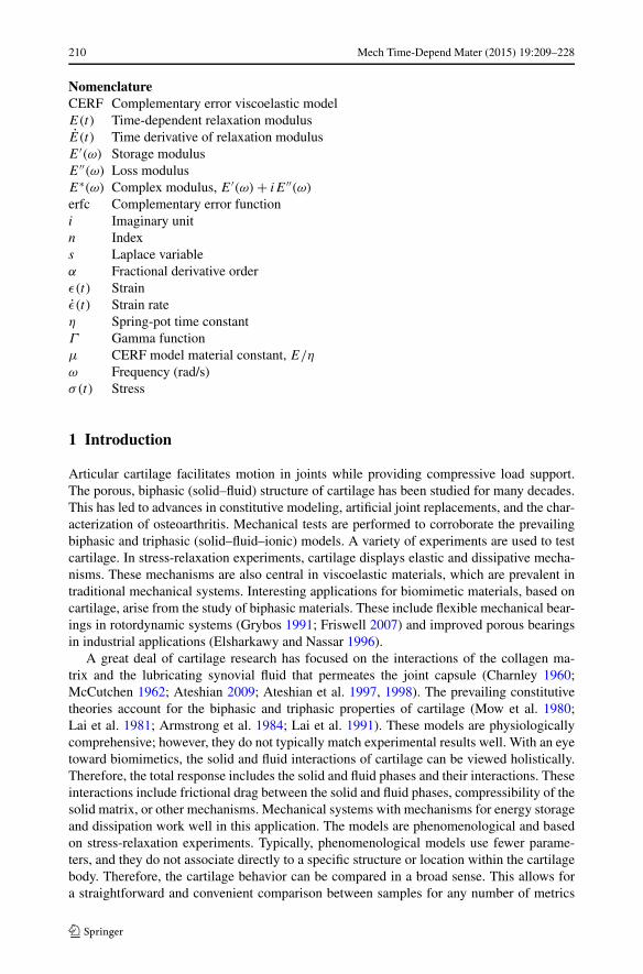
The medial condyle of the right rear stifle is used for study. The stifle joint is mechani-cally analogous to the human knee, and the condyle contains an area of thick and relativelyflat cartilage (approximately 1.5–3 mm thick). After bulk harvesting and resizing of thecondyle, a 10-mm-diameter plug is created with a hollow punch. The punch is driven intothe sample with an arbor press, depicted in Fig. 2. With the punch embedded in the carti-lage and subchrondral bone, the surrounding cartilage is removed with a rotary device. Thepunch has an access hole to allow for hydration of the sample. After the plug is created, itis immersed in saline. The average time from the beginning of dissection to immersion isless than 20 min. The joint capsule is open for approximately 10 min during the process.Previous research highlights the importance of minimizing the exposure time of cartilage toopen-air (Smyth et al. 2014).

214 Mech Time-Depend Mater (2015) 19:209–228

Fig. 2 Schematic of the 10 mmplug creation process

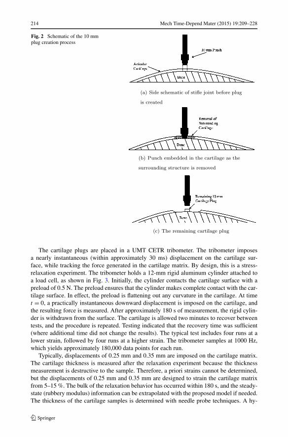
The cartilage plugs are placed in a UMT CETR tribometer. The tribometer imposesa nearly instantaneous (within approximately 30 ms) displacement on the cartilage sur-face, while tracking the force generated in the cartilage matrix. By design, this is a stress-relaxation experiment. The tribometer holds a 12-mm rigid aluminum cylinder attached toa load cell, as shown in Fig. 3. Initially, the cylinder contacts the cartilage surface with apreload of 0.5 N. The preload ensures that the cylinder makes complete contact with the car-tilage surface. In effect, the preload is flattening out any curvature in the cartilage. At timet = 0, a practically instantaneous downward displacement is imposed on the cartilage, andthe resulting force is measured. After approximately 180 s of measurement, the rigid cylin-der is withdrawn from the surface. The cartilage is allowed two minutes to recover betweentests, and the procedure is repeated. Testing indicated that the recovery time was sufficient(where additional time did not change the results). The typical test includes four runs at alower strain, followed by four runs at a higher strain. The tribometer samples at 1000 Hz,which yields approximately 180,000 data points for each run.

Typically, displacements of 0.25 mm and 0.35 mm are imposed on the cartilage matrix.The cartilage thickness is measured after the relaxation experiment because the thicknessmeasurement is destructive to the sample. Therefore, a priori strains cannot be determined,but the displacements of 0.25 mm and 0.35 mm are designed to strain the cartilage matrixfrom 5–15 %. The bulk of the relaxation behavior has occurred within 180 s, and the steady-state (rubbery modulus) information can be extrapolated with the proposed model if needed.The thickness of the cartilage samples is determined with needle probe techniques. A hy-

Mech Time-Depend Mater (2015) 19:209–228 215

Fig. 3 CETR UMT3 tribometerfitted with a 12-mm rigid indenter

podermic needle is attached to the tribometer and travels through the cartilage plug. Thelocations of first contact, surface puncture, and contact with subchondral bone are clearlyshown in the resulting force/displacement graphs. Each test yields a thickness measurement.Multiple measurements are averaged to give a mean thickness, which determines the strainin each sample. The strain is needed to calculate the modulus (discussed herein).

The stress-relaxation experiment is particularly useful because it contains a wide spec-trum of storage and loss properties. Gurtin and Sternberg (1962) developed a constitutivelaw relating stress, strain and the relaxation modulus using Boltzmann’s superposition prin-ciple. The viscoelastic model is time-dependent and retains memory of the material andloading history:

σ(t) = ε(0)E(t) +∫ t

0ε(τ )E(t − τ) dτ, (1)

where σ(t) is the stress, ε(t) is the strain, and E(t) is the relaxation modulus. Typically, σ(t)

and ε(t) are either set or measured during experimentation, whereas E(t) is obtained froma fixed strain input ε = εstep such that E(t) = σ(t)/εstep. The parameters of stress, strain,and elastic modulus in Eq. (1) are time-dependent. It should be noted that Eq. (1) describesa linear relationship between the strain history and the current stress. Transforming Eq. (1)into the Laplace domain allows for simple treatment of the convolution integral:

σ(s) = sE(s)ε(s). (2)

Equation (2) is similar to Hooke’s law in the Laplace domain (for the uniaxial case). Thisprovides the foundation for the elastic–viscoelastic correspondence principle.

To transfer between the Laplace and frequency domains, the Laplace parameter s inEq. (2) is replaced with iω, where i is defined as

√−1, and ω is the frequency in rad/s.Hence, applying s → iω, Eq. (2) becomes

σ(ω) = (iω)E(ω)ε(ω)�= E∗(ω)ε(ω). (3)

E∗(ω) is defined as the complex modulus E∗(ω) = (iω)E(ω) and has two components,a real and an imaginary:

E∗(ω) = E′(ω) + iE′′(ω). (4)

216 Mech Time-Depend Mater (2015) 19:209–228

Fig. 4 Physical representation ofProny series and fractional model

The real component (E′) is known as the storage modulus, whereas the imaginary compo-nent (E′′) is the loss modulus. Both measures describe the dynamic behavior (frequencydependency) of the material, in this case the cartilage. The correspondence principle is pow-erful because one constitutive formulation determines the amount of energy retained (stored)or lost (loss). Stress–strain constitutive equations must be formed that accurately model theexperimental data. One such powerful formulation is the fractional calculus model.

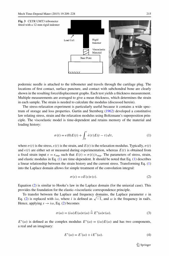
To draw a comparison between the fractional calculus model and more common vis-coelastic models, spring and dashpot systems are considered. Spring and dashpot systemscontain both elastic and dissipative mechanisms simultaneously (Gurtin and Sternberg 1962;Szumski and Green 1991; Miller and Green 1997), which make them appropriate for mod-eling viscoelastic substances. There are many configurations of spring and damper systems,including the Maxwell, Kelvin–Voigt, and Prony series models. The Prony series (Fig. 4(a))is particularly adept in stress-relaxation. However, it often requires many elements to ad-equately model the rapid relaxation seen in cartilage. The fractional calculus model hassimilarities with the Prony series, but the fractional model significantly reduces the numberof elements and thus terms needed to characterize viscoelastic behavior. The model replacesthe dashpot of each Maxwell element with a fractional “spring-pot,” as seen in Fig. 4(b).The spring-pot interpolates between spring and dashpot behavior; in fact, the spring-pot isphysically represented as ladder structure of springs and dashpots (Schiessel and Blumen1993, 1995; Schiessel et al. 1995). Adjusting the constants of the ladder’s “rungs” yieldsany fractional derivative α between 0 and 1. This gives the fractional model great flexibility.A spring-pot is mathematically described as

σsp = ηdαεsp

dtα, (5)

where α is a rational number between 0 and 1, and η is a material parameter similar to adamping coefficient. The parameter η takes on nonstandard units that are similar to viscosity,Pa sα . The interpolative nature of the spring-pot element is clear: if α = 0, then the elementbecomes a spring, and if α = 1, then the element becomes a common viscous dashpot. Forany α between 0 and 1, the element has both spring and dashpot behavior, as described bythe hierarchical analogue (or ladder model) (Schiessel and Blumen 1993, 1995; Schiesselet al. 1995). The virtual increase in mathematical complexity of the fractional model ismitigated by significantly reducing the total terms that are needed to describe the stress/strainrelationship. In comparison to the Prony series, fractional models typically require many

Mech Time-Depend Mater (2015) 19:209–228 217

fewer elements to obtain a similar quality of fit (e.g., in the current study, the fractionalmodel uses 1/4 of the elements of the Prony series). Applying fractional calculus to stress-relaxation, the relaxation modulus can be found in the frequency domain (detailed in theAppendix):

E(ω) = E0

iω+

∞∑n=1

En(iω)α

[(iω)α + En

ηn](

1

iω

). (6)

In the time-domain, the fractional relaxation modulus is (Bagley 1989; Kisela 2009)

E(t) = E0 +∞∑

n=1

EnEα

(−En

ηn

tαn

), (7)

where Eα is the Mittag–Leffler function (Erdelyi et al. 1955),

Eα,β(z) =∞∑

k=0

zk

Γ (αk + β), (8)

and Γ is the gamma function, Γ (x) = (x − 1)!.Whereas the above expression provides a formal time-domain representation, practi-

cally the fractional model is difficult to fit in the time-domain because of convergenceissues. To be practical in modeling, a finite number of terms must be used in the sum-mation in Eq. (8). If the parameter (η) is very small, then k must be very large, andconvergence issues arise. Typically, the fractional model is fit in the frequency domainto circumvent the Mittag–Leffler function; however, the work of Podlubny (1998) pro-poses a Matlab procedure for the Mittag–Leffler function to be fit in the time-domain.The Mittag–Leffler function is avoided altogether in the special case where α = 1/2. Inthis case, the Mittag–Leffler function reduces, and the fractional derivative model effec-tively becomes a complementary error function model (CERF) (Szumski and Green 1991;Szumski 1993) (detailed also in the Appendix). The complementary error function modelis a robust and convenient model for viscoelasticity. It has the advantage of offering a con-cise time-domain solution in the form of the complementary error function multiplied by anexponential function given by

E(t) = E0 +∞∑

n=1

Ene(μn

√t)2

erfc (μn

√t), (9)

where En and μn are material properties, and

μn = En

ηn

. (10)

The complementary error function decays at a faster rate than the exponential increases, giv-ing an overall relaxation behavior. The importance of the CERF model is its time-domainrepresentation. Models with time-domain representations have utility in fitting noisy exper-imental data. The CERF model combines the advantages of the spring and damper models(simple mathematics) with the advantages of the fractional model. This is a very powerfulformulation, which robustly models cartilage with as few as three constants: E0, E1, andμ1 (i.e., only one term (n = 1) in the summation Eq. (9)). Here, μn has nonstandard, but

218 Mech Time-Depend Mater (2015) 19:209–228

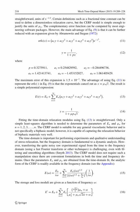
straightforward, units of s−1/2. Certain definitions such as a fractional time constant can beused to define a dimensionless relaxation curve, but the CERF model is simple enough tojustify the units of μn. The complementary error function can be computed by most engi-neering software packages. However, the main advantage of Eq. (9) is that it can be furtherreduced with an expansion given by Abramowitz and Stegun (1972):

erfc(x) = (a1y + a2y

2 + a3y3 + a4y

4 + a5y5)e−x2

, (11)

y = 1

1 + px, (12)

where

p = 0.3275911, a1 = 0.254829592, a2 = −0.284496736,

a3 = 1.421413741, a4 = −1.453152027, a5 = 1.061405429.

The maximum error of this expansion is 1.5 × 10−7. The advantage of using Eq. (11) torepresent the erfc(·) in Eq. (9) is that the exponentials cancel out as x = μ

√t . The result is

a simple polynomial expression:

E(t) = E0 +∞∑

n=1

En

(a1y + a2y

2 + a3y3 + a4y

4 + a5y5), (13)

y = 1

1 + μp√

t. (14)

Fitting the time-domain relaxation modulus using Eq. (13) is straightforward. Only asimple least-squares algorithm is needed to determine the parameters of En and μn forn = 1,2,3, . . . , n. The CERF model is suitable for any general viscoelastic behavior and isnot specifically a biphasic model; however, it is capable of capturing the relaxation behaviorof biphasic materials very well.

The time-domain is important for performing experiments and qualitative understandingof stress-relaxation, but the frequency domain is fundamental to a dynamic analysis. How-ever, transferring the quite noisy raw experimental signal from the time to the frequencydomain (using a fast Fourier transform or other techniques) is challenging, even with fil-tering and smoothing algorithms (Smyth 2013). The CERF model does not require such amanipulation since there are convenient formulations in both the time and frequency do-mains. Once the parameters En and μn are obtained from the time-domain fit, the analyticform of the CERF is readily available in the frequency domain (see the Appendix):

E(ω) = E0

iω+

∞∑n=1

En(iω)1/2

[(iω)1/2 + En

ηn](

1

iω

). (15)

The storage and loss moduli are given as a function of frequency ω:

E′ = E0 +∞∑

n=1

En

[ (√2ω2

)μn + ω

μ2n + μn

√2ω + ω

], (16)

Mech Time-Depend Mater (2015) 19:209–228 219

Table 1 Comparison data for CERF and Prony series (n = 1)

CERF Prony

E0 (MPa) 1.409 0.774

E1 (MPa) 0.549 0.677

μ21 or λ1 (1/s) μ2

1 = 0.8649 × 10−2 λ1 = 0.410 × 10−1

E′′ =∞∑

n=1

En

[ (√2ω2

)μn

μ2n + μn

√2ω + ω

]. (17)

3 Results

The CERF model (n = 1, Eq. (13)) is fit to the relaxation behavior, which is pronounced inthe initial time of the experiment (Fig. 5(a)). In addition, the Prony series model (Eq. (18),n = 1) is also shown in Fig. 5(a) as a comparison to the CERF model (see Table 1 for fitparameters).

EProny(t) = E0 +∞∑

n=1

Ene−λnt . (18)

The Prony model is fit in a similar least-squares manner and contains the same number ofconstants as the CERF. When n = 1, the Prony series is known as the standard linear solid(Smyth 2013). Clearly, the standard linear model is unable to capture the relaxation in thefirst 100 s of decay, rendering it of little use in the current study. The relaxation behavioris captured well with the CERF model (n = 1, which is the CERF equivalent to a standardlinear solid). Only minor deviation between the fit and the actual data is seen in both scalesin Fig. 5. The deviation between the model and experimental data corresponds to the highestfrequency information. For horses (and humans), frequency ranges greater than 4–5 Hz arenot accessed during even the most strenuous exercises. Therefore, it is less important tocapture this corresponding region of the relaxation data, i.e., from t = 0 s to t = 200 ms.The CERF robustly models the important decades of relaxation behavior (shown in Fig. 5(b)using a semi-log scale), which makes its utility apparent for biological materials. The CERFmodel is powerful in that only three parameters, E0, E1, and μ1 (corresponding to n = 1), areneeded to robustly fit the bulk relaxation behavior. In applications where biphasic materialsare integrated into larger system dynamics, this compact model has great utility.

The frequency domain allows for study of cartilage as a function of gait. The elastic–viscoelastic correspondence principle transfers time-dependent information to the Laplaceand frequency domains without loss of generality. Therefore, stress-relaxation experimentsgive directly the storage and loss moduli as functions of frequency ω. A comparison of theCERF and Prony series models (n = 1) in the frequency domain is shown in Fig. 6 for thestorage and loss modulus. The two models have significant differences over many frequencydecades. Considering the storage modulus (Fig. 6(a)), the CERF and Prony models displaylarge differences, particularly at low frequencies. Likewise, the loss modulus (Fig. 6(b)) hasmajor differences (nearly an order of magnitude in the physiological range), indicating thatthe two models are fundamentally different. Based on the relaxation seen in Fig. 5, the CERFdescribes the frequency behavior of cartilage more accurately.

220 Mech Time-Depend Mater (2015) 19:209–228

Fig. 5 Example fit of CERF tostress-relaxation experiment ofcartilage plug immersed in saline

Analysis in the frequency domain shows that cartilage has strong frequency characteris-tics. Common gaits for cartilage are in the viscoelastic transition region, which is betweenthe higher frequencies giving the glassy region (4 Hz) and the lower frequencies giving therubbery region (0.25 Hz). Cartilage adjusts to a stimulus by storing and dissipating differ-ent amounts of energy, depending on the frequency of perturbation. This is potentially animportant characteristic of biphasic materials. The adaptive nature of cartilage is well suitedfor bioinspired designs of bearings and dampers.

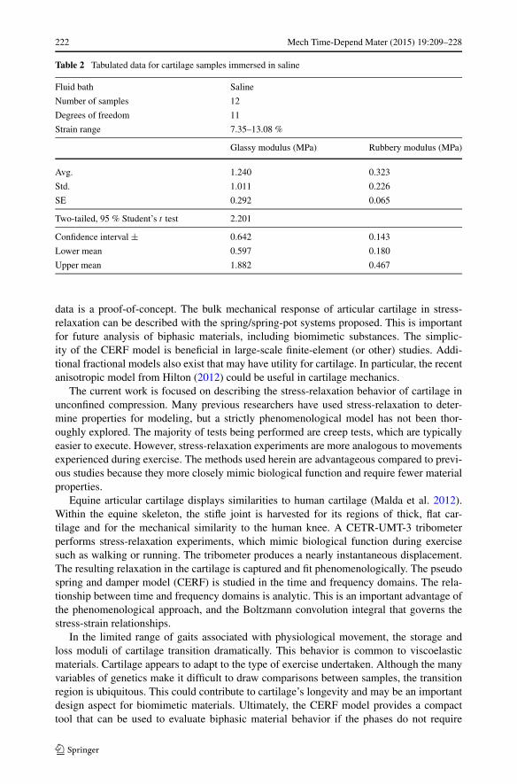
The thickness of the cartilage plugs is not known a priori. This complicates the analysisas the testing procedure imposed a predetermined displacement on the cartilage sample.The strain is determined by the thickness of the sample. Therefore, results obtained fromthe relaxation experiments are inherently over a range of strains. Attempts were made tolimit the strains to 5–15 %; however, there are a few cases where 15 % is exceeded. Eachmeasurement is fit with Eq. (9) to determine the parameters E0, E1, and μ1. An examplefit of the CERF (n = 1) to actual cartilage relaxation data is shown in Fig. 5. When t = 0,the glassy modulus is obtained (Eglassy = E0 + E1), and as t → ∞, the rubbery modulusis found (Erubbery = E0). These quantities are reported in the vertical columns of Table 2.Student’s t test is used to provide upper and lower bounds for the respective moduli. It isdifficult to generalize all of the samples as one conglomerate; however, this is provided as anestimate of the glassy and rubbery moduli. The combined results represent a range of likelycartilage behavior, and each sample is said to have certain strain-dependent properties. Moreexhaustive testing and additional data should be used to corroborate this finding. The large

Mech Time-Depend Mater (2015) 19:209–228 221

Fig. 6 Comparison of the CERFand Prony models in thefrequency domain

standard deviation and error seen in Table 2 is likely due to a relatively small sample sizeand large variability in samples due to age, breed, use, etc.

Large variations are expected in biological samples. Each cartilage explant is unique,which increases the difficulty of drawing meaningful conclusions from the data. Genetics,weight, age, diet, gender, and use can influence the mechanical properties of cartilage. Themodel parameters obtained from experiments are expected to have large variations. How-ever, a prevailing trend is that the transition period of cartilage coincides with the physi-ological range of exercise. At lower frequencies, cartilage dissipates more energy than athigher frequencies, where additional elasticity is available in the joints. The transition rangeof cartilage occurs in the middle of the common frequencies of motion (0.25–4 Hz). It ispossible that the adaptive nature of cartilage is biologically designed for this purpose.

4 Discussion

A simple model that describes the behavior of cartilage is proposed. Under the specifiedloading (stress-relaxation), the CERF model is able to account for biphasic behavior whenconsidered as a conglomerate material. Many additional tests are required to quantitativelydescribe the behavior of equine cartilage. The CERF model does have limitations; however,its application is appropriate in many situations. In particular, the CERF model has utilityin impact studies, adaptive bearings and dampers design, and study of systems that includebiphasic materials.

The preliminary results obtained should justify additional research and experimentation.More cartilage samples are needed for statistical significance; however, the experimental

222 Mech Time-Depend Mater (2015) 19:209–228

Table 2 Tabulated data for cartilage samples immersed in saline

Fluid bath Saline

Number of samples 12

Degrees of freedom 11

Strain range 7.35–13.08 %

Glassy modulus (MPa) Rubbery modulus (MPa)

Avg. 1.240 0.323

Std. 1.011 0.226

SE 0.292 0.065

Two-tailed, 95 % Student’s t test 2.201

Confidence interval ± 0.642 0.143

Lower mean 0.597 0.180

Upper mean 1.882 0.467

data is a proof-of-concept. The bulk mechanical response of articular cartilage in stress-relaxation can be described with the spring/spring-pot systems proposed. This is importantfor future analysis of biphasic materials, including biomimetic substances. The simplic-ity of the CERF model is beneficial in large-scale finite-element (or other) studies. Addi-tional fractional models also exist that may have utility for cartilage. In particular, the recentanisotropic model from Hilton (2012) could be useful in cartilage mechanics.

The current work is focused on describing the stress-relaxation behavior of cartilage inunconfined compression. Many previous researchers have used stress-relaxation to deter-mine properties for modeling, but a strictly phenomenological model has not been thor-oughly explored. The majority of tests being performed are creep tests, which are typicallyeasier to execute. However, stress-relaxation experiments are more analogous to movementsexperienced during exercise. The methods used herein are advantageous compared to previ-ous studies because they more closely mimic biological function and require fewer materialproperties.

Equine articular cartilage displays similarities to human cartilage (Malda et al. 2012).Within the equine skeleton, the stifle joint is harvested for its regions of thick, flat car-tilage and for the mechanical similarity to the human knee. A CETR-UMT-3 tribometerperforms stress-relaxation experiments, which mimic biological function during exercisesuch as walking or running. The tribometer produces a nearly instantaneous displacement.The resulting relaxation in the cartilage is captured and fit phenomenologically. The pseudospring and damper model (CERF) is studied in the time and frequency domains. The rela-tionship between time and frequency domains is analytic. This is an important advantage ofthe phenomenological approach, and the Boltzmann convolution integral that governs thestress-strain relationships.

In the limited range of gaits associated with physiological movement, the storage andloss moduli of cartilage transition dramatically. This behavior is common to viscoelasticmaterials. Cartilage appears to adapt to the type of exercise undertaken. Although the manyvariables of genetics make it difficult to draw comparisons between samples, the transitionregion is ubiquitous. This could contribute to cartilage’s longevity and may be an importantdesign aspect for biomimetic materials. Ultimately, the CERF model provides a compacttool that can be used to evaluate biphasic material behavior if the phases do not require

Mech Time-Depend Mater (2015) 19:209–228 223

separation. The CERF is not a detailed model for cartilage, but it allows for practical analysisto be undertaken.

Unconfined compression tests and the CERF model can characterize cartilage with asfew as two types of terms: E and μ. Poisson’s ratio and other experimental “fudge-factors”are not required for fitting the data. For a complex material, models that can capture themajority of the mechanical response with relatively few parameters are very useful. Theadvantage of the phenomenological characterization is its simplicity. The techniques givencan be used for comparisons between species or between healthy and diseased cartilage. Thematerial properties given are needed for a full dynamic or impact study. Potential other usesof the CERF include: magnetic resonance elastography (MRE), biphasic bearing/damperevaluation, and control problems considering fractional order viscoelasticity.

5 Conclusions

There has been little previous work linking fractional calculus and biomechanics, and inparticular, cartilage mechanics. However, as displayed in the current study, the robustnessand flexibility of fractional calculus is well suited for such applications. The special caseof fractional derivative, α = 1/2, has unique advantages for modeling stress-relaxation incartilage. The time-domain representation of the CERF model (Eq. (13)) is very powerfuland intrinsically useful when the elastic-viscoelastic correspondence principle is invoked.For the first time, it is shown that the relaxation modulus can be robustly expressed as apolynomial, and the polynomial expansion is easily fit in a least-squares sense. This aloneis advantageous when compared to many models that present significant fitting challenges.The succinctness of the CERF model is a major factor in its utility. In applications wherecartilage (or a biphasic material in general) is modeled as a component of a larger system, theCERF model is accurate without being inordinate. These reasons warrant additional studyin fractional calculus and biomechanics.

Acknowledgements This work is supported by NSF Grant No. DGE-1148903.

Appendix

For simplicity, only a one-element fractional derivative model is developed. However, theone-element model can be generalized to include multiple elements in parallel by the prin-ciple of linear superposition. This concept is analogous to that of the more common Pronyseries. The constitutive equation relating stress to strain is similar to that of a standard linearviscoelastic material:

(1 + E0

E1

)dε

dt+ E0

c1ε = 1

E1

dσ

dt+ 1

c1σ, (A.1)

except that the dashpot is replaced with the spring-pot element

dε

dt←− dαε

dtα(A.2)

and

dσ

dt←− dασ

dtα, (A.3)

224 Mech Time-Depend Mater (2015) 19:209–228

leading to the constitutive equation for the fractional derivative model(

1 + E0

E1

)dαε

dtα+ E0

η1ε = 1

E1

dασ

dtα+ 1

η1σ. (A.4)

In Eq. (A.4), the damping coefficient c1 has been replaced by η1 to reflect unit consistency.If α = 1, then the constitutive model becomes the standard linear material (one-term Pronymodel shown in Eq. (A.1)), and the units of η1 collapse to those of c1 (Pa s). If α = 0,then the spring-pot simply becomes strictly a spring, and the entire model is reduced to anequivalent linear spring. For any fractional valued α between 0 and 1, the spring-pot elementhas both spring and dashpot behavior.

Equation (A.4) is conveniently analyzed in the Laplace domain, which allows for thetreatment of the fractional power (taking Caputo’s definition of the fractional-order deriva-tive and assuming that the initial conditions for stress and strain can be set to zero (Podlubny1998)):

[(1 + E0

E1

)sα + E0

η1

]ε(s) =

(1

E1sα + 1

η1

)σ(s). (A.5)

Utilizing the elastic–viscoelastic correspondence principle (Eq. (2)), the relaxation modulusE(s) can be found from Eq. (A.5):

E(s) =[(

1 + E0E1

)sα + E0

η1

]( 1

E1sα + 1

η1)

1

s. (A.6)

The relationship between the Laplace and frequency domains allows for the fractional modelto be obtained:

E(ω) =[(

1 + E0E1

)(iω)α + E0

η1

][ 1

E1(iω)α + 1

η1]

(1

iω

). (A.7)

With some algebra, Eq. (A.7) can be reduced to

E(ω) = 1

iω

[E0 + E1(iω)α[

(iω)α + E1η1

]]. (A.8)

If required, the fractional model can be generalized to include more spring-pot elements:

E(ω) = 1

iω

[E0 +

∞∑n=1

En(iω)α[(iω)α + En

ηn

]]. (A.9)

Theoretically, an infinite number of terms can be used. In practice, this number is finite. Thecomplex modulus is found from the elastic–viscoelastic correspondence principle (Eq. (2)):

E∗(ω) = E0 +∞∑

n=1

En(iω)α[(iω)α + En

ηn

] . (A.10)

Simplifications for α = 1/2 (special case)For the special case of α = 1/2, the mathematics of the fractional model simplify dra-

matically. In the time domain, a concise solution appears in the form of a complementary

Mech Time-Depend Mater (2015) 19:209–228 225

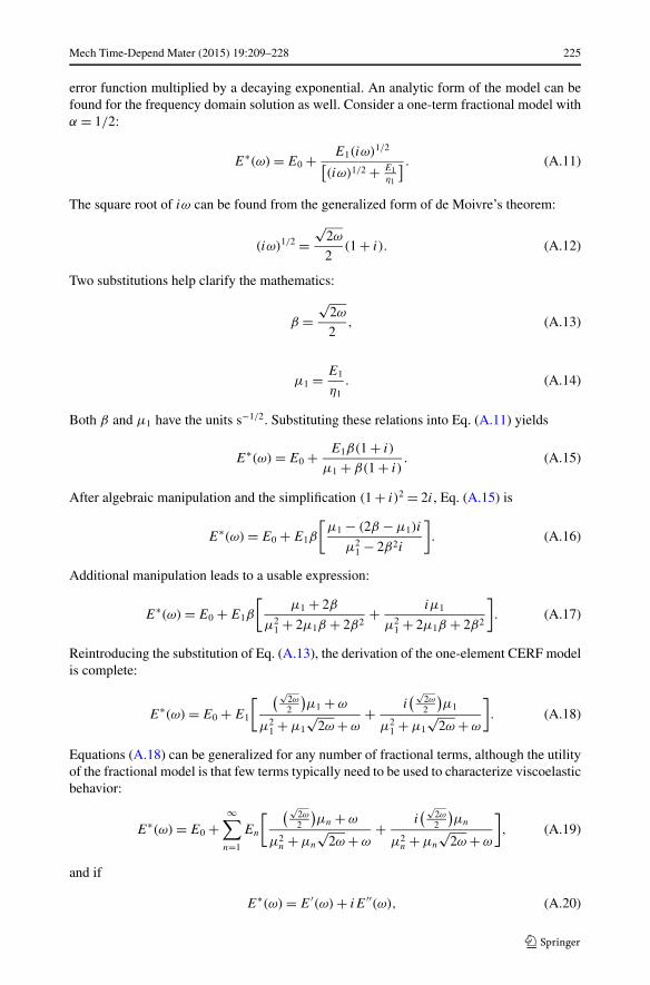
error function multiplied by a decaying exponential. An analytic form of the model can befound for the frequency domain solution as well. Consider a one-term fractional model withα = 1/2:

E∗(ω) = E0 + E1(iω)1/2[(iω)1/2 + E1

η1

] . (A.11)

The square root of iω can be found from the generalized form of de Moivre’s theorem:

(iω)1/2 =√

2ω

2(1 + i). (A.12)

Two substitutions help clarify the mathematics:

β =√

2ω

2, (A.13)

μ1 = E1

η1. (A.14)

Both β and μ1 have the units s−1/2. Substituting these relations into Eq. (A.11) yields

E∗(ω) = E0 + E1β(1 + i)

μ1 + β(1 + i). (A.15)

After algebraic manipulation and the simplification (1 + i)2 = 2i, Eq. (A.15) is

E∗(ω) = E0 + E1β

[μ1 − (2β − μ1)i

μ21 − 2β2i

]. (A.16)

Additional manipulation leads to a usable expression:

E∗(ω) = E0 + E1β

[μ1 + 2β

μ21 + 2μ1β + 2β2

+ iμ1

μ21 + 2μ1β + 2β2

]. (A.17)

Reintroducing the substitution of Eq. (A.13), the derivation of the one-element CERF modelis complete:

E∗(ω) = E0 + E1

[ (√2ω2

)μ1 + ω

μ21 + μ1

√2ω + ω

+ i(√

2ω2

)μ1

μ21 + μ1

√2ω + ω

]. (A.18)

Equations (A.18) can be generalized for any number of fractional terms, although the utilityof the fractional model is that few terms typically need to be used to characterize viscoelasticbehavior:

E∗(ω) = E0 +∞∑

n=1

En

[ (√2ω2

)μn + ω

μ2n + μn

√2ω + ω

+ i(√

2ω2

)μn

μ2n + μn

√2ω + ω

], (A.19)

and if

E∗(ω) = E′(ω) + iE′′(ω), (A.20)

226 Mech Time-Depend Mater (2015) 19:209–228

then

E′(ω) = E0 +∞∑

n=1

En

[ (√2ω2

)μn + ω

μ2n + μn

√2ω + ω

], (A.21)

E′′(ω) =∞∑

n=1

En

[ (√2ω2

)μn

μ2n + μn

√2ω + ω

]. (A.22)

For the fractional derivative model where α = 1/2, there exists a concise time-domainsolution (Szumski and Green 1991):

E(t) = E0 +∞∑

n=1

Ene(μn

2t)erfc (μn

√t), (A.23)

which is a decaying complementary error function multiplied by an increasing exponential.The time-domain solution is critical for fitting experimental data. The Laplace transforma-tion of Eq. (9) is given by Szumski and Green (1991):

E(s) = 1

s

[E0 +

∞∑n=1

En

√s√

s + μn

]. (A.24)

Equation (A.24) and application of the elastic–viscoelastic correspondence principle allowsus to relate the CERF model in the time and frequency domains, noting the connectionbetween the Laplace and Fourier transformations (replace the Laplace variable s with theFourier variable iω). We then arrive back at Eq. (A.19).

References

Erdelyi, A., Oberhettinger, F., Magnus, W., Tricomi, F. (eds.): Higher Transcendental Functions, vol. III.McGraw-Hill, New York (1955)

Abramowitz, M., Stegun, I.A. (eds.): Handbook of Mathematical Functions. Dover, New York (1972)Argatov, I.I.: Mathematical modeling of linear viscoelastic impact: application to drop impact testing of

articular cartilage. Tribol. Int. 63, 213–225 (2013)Armstrong, C.G., Lai, W.M., Mow, V.C.: An analysis of the unconfined compression of articular cartilage.

J. Biomech. Eng. 106(2), 165–173 (1984)Ateshian, G.A.: The role of interstitial fluid pressurization in articular cartilage lubrication. J. Biomech. 42(9),

1163–1176 (2009)Ateshian, G.A., Warden, W.H., Kim, J.J., Grelsamer, R.P., Mow, V.C.: Finite deformation biphasic material

properties of bovine articular cartilage from confined compression experiments. J. Biomech. 30(11–12),1157–1164 (1997)

Ateshian, G.A., Wang, H., Lai, W.M.: The role of interstitial fluid pressurization and surface porosities on theboundary friction of articular cartilage. J. Tribol. 120(2), 241–248 (1998)

Bagley, R.L.: Power law and fractional calculus model of viscoelasticity. AIAA J. 27(10), 1412–1417 (1989)Bagley, R.L., Torvik, P.J.: A generalized derivative model for an elastomer damper. Shock Vibr. Bull. 49(2),

135–143 (1979)Bagley, R.L., Torvik, P.J.: A theoretical basis for the application of fractional calculus to viscoelasticity.

J. Rheol. 27(3), 201–210 (1983).Bagley, R.L., Torvik, P.J.: Fractional calculus in the transient analysis of viscoelastically damped structures.

AIAA J. 23(6), 918–925 (1985)Bagley, R.L., Torvik, P.J.: On the fractional calculus model of viscoelastic behavior. J. Rheol. 30(1), 133–155

(1986)

Mech Time-Depend Mater (2015) 19:209–228 227

Carpinteri, A., Mainardi, F.: Fractals and Fractional Calculus in Continuum Mechanics. Courses and Lec-tures/International Centre for Mechanical Sciences/International Centre for Mechanical Sciences Udine,vol. 378. Springer, London (1997)

Charnley, J.: The lubrication of animal joints in relation to surgical reconstruction by arthroplasty. Ann.Rheum. Dis. 19, 10–19 (1960)

Coletti, J.M., Akeson, W.H., Woo, S.L.Y.: A comparison of the physical behavior of normal articular cartilageand the arthroplasty surface. J. Bone Jt. Surg. 54-A(1), 147–160 (1972)

DiSilvestro, M.R., Suh, J.K.F.: A cross-validation of the biphasic poroviscoelastic model of articular cartilagein unconfined compression, indentation, and confined compression. J. Biomech. 34(4), 519–525 (2001)

Ehlers, W., Markert, B.: A linear viscoelastic two-phase model for soft tissues: application to articular carti-lage. Z. Angew. Math. Mech. 80(S1), 149–152 (2000)

Ehlers, W., Markert, B.: A linear viscoelastic biphasic model for soft tissues based on the theory of porousmedia. J. Biomech. Eng. 123(5), 418–424 (2001)

Eisenfeld, J., Mow, V.C., Lipshitz, H.: Mathematical analysis of stress relaxation in articular cartilage duringcompression. Math. Biosci. 39(1–2), 97–112 (1978)

Elsharkawy, A.A., Nassar, M.M.: Hydrodynamic lubrication of squeeze-film porous bearings. Acta Mech.118, 121–134 (1996)

Friswell, M.: The response of rotating machines on viscoelastic supports. Int. Rev. Mec. Eng. 1(1), 32–40(2007)

Fung, Y.C.: Elasticity of soft tissues in simple elongation. Am. J. Physiol. 213(6), 1532–1544 (1967)Garcia, J.J., Cortes, D.H.: A nonlinear biphasic viscohyperelastic model for articular cartilage. J. Biomech.

39(16), 2991–2998 (2006)Grybos, G.R.: The dynamics of a viscoelastic rotor in flexible bearings. Arch. Appl. Mech. 61(1), 479–487

(1991)Gurtin, M.E., Sternberg, E.: On the linear theory of viscoelasticity. Arch. Ration. Mech. Anal. 11(1), 291–356

(1962)Hilton, H.H.: Generalized fractional derivative anisotropic viscoelastic characterization. Materials 5(1), 169–

191 (2012). doi:10.3390/ma5010169Julkunen, P., Wilson, W., Jurvelin, J.S., Rieppo, J., Qu, C.J., Lammi, M.J., Korhonen, R.K.: Stress relaxation

of human patellar articular cartilage in unconfined compression: prediction of mechanical response bytissue composition and structure. J. Biomech. 41(9), 1978–1986 (2008)

Kisela, T.: Fractional generalization of the classical viscoelasticity models. In: Proceedings of 8th Interna-tional Conference Aplimat 2009, pp. 593–600 (2009)

Koeller, R.: Applications of fractional calculus to the theory of viscoelasticity. J. Appl. Mech. 51, 299–307(1984)

Koeller, R.C.: Polynomial operators, Stieltjes convolution, and fractional calculus in hereditary mechanics.Acta Mech. 58(3–4), 251–264 (1986)

Lai, W.M., Mow, V.C., Roth, V.: Effects of nonlinear strain-dependent permeability and rate of compressionon the stress behavior of articular cartilage. J. Biomech. Eng. 103(2), 61–66 (1981)

Lai, W.M., Hou, J.S., Mow, V.C.: A triphasic theory for the swelling and deformation behaviors of articularcartilage. J. Biomech. Eng. 113(3), 245–258 (1991)

Lakes, R.: Viscoelastic Solids. Mechanical and Aerospace Engineering Series. Taylor & Francis, London(1998)

Magin, R.: Fractional Calculus in Bioengineering. Begell House Publishers, Readding (2006)Mainardi, F., Spada, G.: Creep, relaxation and viscosity properties for basic fractional models in rheology.

Eur. Phys. J. Spec. Top. 193(1), 133–160 (2011)Mak, A.F.: The apparent viscoelastic behavior of articular cartilage—the contributions from the intrinsic

matrix viscoelasticity and interstitial fluid flows. J. Biomech. Eng. 108(2), 123–130 (1986)Malda, J., Benders, K.E.M., Klein, T.J., de Grauw, J.C., Kik, M.J.L., Hutmacher, D.W., Saris, D.B.F., van

Weeren, P.R., Dhert, W.J.A.: Comparative study of depth-dependent characteristics of equine and humanosteochondral tissue from the medial and lateral femoral condyles. Osteoarthr. Cartil. 20(10), 1147–1151 (2012)

McCutchen, C.W.: The frictional properties of animal joints. Wear 5(1), 1–17 (1962)Miller, B., Green, I.: On the stability of gas lubricated triboelements using the step jump method. J. Tribol.

119(1), 193–199 (1997)Mow, V., Gu, W., Chen, F.: Structure and Function of Articular Cartilage and Meniscus. In: Basic Orthopaedic

Biomechanics & Mechano-Biology, 3rd edn., pp. 181–258. Lippincott Williams & Wilkins, Philadel-phia (2005)

Mow, V.C., Mansour, J.M.: The nonlinear interaction between cartilage deformation and interstitial fluid flow.J. Biomech. 10(1), 31–39 (1977)

228 Mech Time-Depend Mater (2015) 19:209–228

Mow, V.C., Lipshitz, H., Glimcher, M.J.: Mechanisms for stress relaxation in articular cartilage. In: 23rd An-nual Meeting of the Orthopaedic Research Society, Las Vegas, vol. 2, p. 71. The Orthopaedic ResearchSociety, Rosemont (1977)

Mow, V.C., Kuei, S.C., Lai, W.M., Armstrong, C.G.: Biphasic creep and stress relaxation of articular cartilagein compression: theory and experiments. J. Biomech. Eng. 102(1), 73–84 (1980)

Mow, V.C., Ateshian, G.A., Spilker, R.L.: Biomechanics of diarthrodial joints: a review of twenty years ofprogress. J. Biomech. Eng. 115(4B), 460–467 (1993)

Parsons, J.R., Black, J.: The viscoelastic shear behavior of normal rabbit articular cartilage. J. Biomech. 10(1),21–29 (1977)

Podlubny, I.: Fractional Differential Equations: An Introduction to Fractional Derivatives, Fractional Differ-ential Equations, to Methods of Their Solution and Some of Their Applications. Mathematics in Scienceand Engineering, Elsevier, Amsterdam (1998)

Rogers, L.: Operators and fractional derivatives for viscoelastic constitutive equations. J. Rheol. 27(4), 351–372 (1983)

Schiessel, H., Blumen, A.: Hierarchical analogues to fractional relaxation equations. J. Phys. A, Math. Gen.26(19), 5057 (1993)

Schiessel, H., Blumen, A.: Mesoscopic pictures of the sol-gel transition: ladder models and fractal net-works. Macromolecules 28(11), 4013–4019 (1995). http://pubs.acs.org/doi/pdf/10.1021/ma00115a038.doi:10.1021/ma00115a038

Schiessel, H., Metzler, R., Blumen, A., Nonnenmacher, T.F.: Generalized viscoelastic models: their fractionalequations with solutions. J. Phys. A, Math. Gen. 28(23), 6567 (1995)

Simon, B.R., Coats, R.S., Woo, S.L.Y.: Relaxation and creep quasilinear viscoelastic models for normalarticular cartilage. J. Biomech. Eng. 106(2), 159–164 (1984)

Smyth, P.: Viscoelastic behavior of articular cartilage in unconfined compression. Master’s thesis, GeorgiaInstitute of Technology (2013)

Smyth, P.A., Rifkin, R.E., Jackson, R.L., Reid Hanson, R.: The average roughness and fractal dimension ofarticular cartilage during drying. Scanning 36(3), 368–375 (2014)

Szumski, R.G.: A finite element formulation for the time domain vibration analysis of an elastic-viscoelasticstructure. Ph.D. thesis, Georgia Institute of Technology (1993)

Szumski, R.G., Green, I.: Constitutive laws in time and frequency domains for linear viscoelastic materials.J. Acoust. Soc. Am. 90(40), 2292 (1991)

Tanaka, E., Pelayo, F., Kim, N., Lamela, M.J., Kawai, N., Fernãndez-Canteli, A.: Stress relaxation behaviorsof articular cartilages in porcine temporomandibular joint. J. Biomech. 47(7), 1582–1587 (2014)

Torvik, P.J., Bagley, R.L.: On the appearance of the fractional derivative in the behavior of real materials.J. Appl. Mech. 51(2), 294–298 (1984)

Wang, J.L., Parnianpour, M., ShiraziAdl, A., Engin, A.E.: Failure criterion of collagen fiber: viscoelasticbehavior simulated by using load control data. Theor. Appl. Fract. Mech. 27(1), 1–12 (1997)

West, B., Bologna, M., Grigolini, P.: Physics of Fractal Operators. Institute for Nonlinear Science/Springer,Berlin (2003)

Wilson, W., van Donkelaar, C.C., van Rietbergen, B., Ito, K., Huiskes, R.: Stresses in the local collagennetwork of articular cartilage: a poroviscoelastic fibril-reinforced finite element study. J. Biomech. 37(3),357–366 (2004)

Wilson, W., van Donkelaar, C.C., van Rietbergen, B., Huiskes, R.: A fibril-reinforced poroviscoelasticswelling model for articular cartilage. J. Biomech. 38(6), 1195–1204 (2005)

Woo, S.L.Y., Simon, B.R., Kuei, S.C., Akeson, W.H.: Quasi-linear viscoelastic properties of normal articularcartilage. J. Biomech. Eng. 102(2), 85–90 (1980)