Embed Size (px)
Citation preview
Fraction-free Row Reduction of Matrices of
Ore Polynomials
Bernhard Beckermann a Howard Cheng b George Labahn c
aLaboratoire Painleve UMR 8524 (ANO-EDP), UFR Mathematiques – M3, USTLille, F-59655 Villeneuve d’Ascq CEDEX, France
bDepartment of Mathematics and Computer Science, University of Lethbridge,Lethbridge, Alberta, Canada, T1K 3M4
cSchool of Computer Science, University of Waterloo, Waterloo, Ontario, Canada,N2L 3G1
Abstract
In this paper we give formulas for performing row reduction of a matrix of Orepolynomials in a fraction-free way. The reductions can be used for finding the rankand left nullspace of such matrices. When specialized to matrices of skew polyno-mials our reduction can be used for computing a weak Popov form of such matricesand for computing a GCRD and an LCLM of skew polynomials or matrices of skewpolynomials. The algorithm is suitable for computation in exact arithmetic domainswhere the growth of coefficients in intermediate computations is a concern. This co-efficient growth is controlled by using fraction-free methods. The known factor canbe predicted and removed efficiently.
1 Introduction
Ore rings provide a general setting for describing linear differential, recurrence,difference and q-difference operators. Formally these are given by IK [Z;σ, δ]with IK a field of coefficients, Z an indeterminate, σ an injective homomor-phism, δ a derivation and with the multiplication rule Za = σ(a)Z + δ(a) forall a ∈ IK . In this paper we are interested in matrices of Ore polynomials andlook at the problem of transforming such matrices into “simpler” ones using
Email addresses: [email protected] (Bernhard Beckermann),[email protected] (Howard Cheng), [email protected] (GeorgeLabahn).
Preprint submitted to Elsevier Science 27 September 2005
only certain row operations. Examples of such transformations include con-version to special forms, such as row-reduced, Popov or weak Popov normalforms. In our case we are primarily interested in transformations which allowfor easy determination of rank and left nullspaces.
For a given m× s matrix F(Z) ∈ IK [Z;σ, δ]m×s we are interested in applyingtwo types of elementary row operations. The first type includes
(a) interchange two rows;(b) multiply a row by a nonzero element in IK [Z;σ, δ] on the left;(c) add a polynomial left multiple of one row to another.
In the second type of elementary row operations we include (a), (b) and (c)but require that the row multiplier in (b) comes from IK . The second set ofrow operations is useful, for example, when computing a Greatest CommonRight Divisor (GCRD) or a Least Common Left Multiple (LCLM) of Orepolynomials.
Formally, in the first instance we can view a sequence of elementary row op-erations as a matrix U(Z) ∈ IK [Z;σ, δ]m×m with the result of these row op-erations given by T(Z) = U(Z) F(Z) ∈ IK [Z;σ, δ]m×s. In the second case,U(Z) would have the additional property that there exists a left inverseV(Z) ∈ IK [Z;σ, δ]m×m such that V(Z) U(Z) = Im. In the commutative case,such a transformation matrix is called unimodular [Kailath, 1980].
In many cases it is possible to transform via row operations a matrix of Orepolynomials into one whose rank is completely determined by the rank of itsleading or trailing coefficient. In the commutative case, this can be done viaan algorithm of Beckermann and Labahn [1997] while in the noncommutativecase of skew polynomials (i.e. where δ = 0) this can be done using eitherthe EG-elimination method of Abramov [1999] or the algorithm of Abramovand Bronstein [2001]. In the commutative case, examples of applications forsuch transformations include matrix polynomial division, inversion of matrixpolynomials, finding matrix GCDs of two matrix polynomials and finding allsolutions to various rational approximation problems. For the skew polynomialcase, it was shown by Abramov and Bronstein [2001] that such transformationscan be used to find polynomial and rational solutions of linear functionalsystems.
The algorithm given by Abramov and Bronstein [2001] improves on the EG-elimination method of Abramov [1999] and extends a method of Beckermannand Labahn [1997] to the noncommutative case. While these algorithms havegood arithmetic complexity, coefficient growth may occur and can only becontrolled through coefficient GCD computations. Without such GCD com-putations the coefficient growth can be exponential. Examples of such growthcan be found in Section 8.
2
In this paper we consider the problem of determining the rank and left nullspaceof a matrix of Ore polynomials for problems where coefficient growth is an is-sue. Our aim is to give a fraction-free algorithm for finding these quantitieswhen working over the domain ID [Z;σ, δ] with ID an integral domain, andσ(ID ) ⊂ ID , δ(ID ) ⊂ ID . Examples of such domains include ID = IF [n] forsome field IF with Z the shift operator and ID = IF [x] and where Z is thedifferential operator. By fraction-free we mean that we can work entirely inthe domain ID [Z;σ, δ] but that coefficient growth is controlled without anyneed for costly coefficient GCD computations. In addition we want to ensurethat all intermediate results can be bounded in size which allows for a preciseanalysis of the growth of coefficients of our computation.
Our results extend the algorithm of Beckermann and Labahn [2000] in thecommutative case and Beckermann et al. [2002] in the case of matrices ofskew polynomials. This extension has considerable technical challenges. Forexample, unlike the skew and commutative polynomial case, the rank is nolonger necessarily determined by the rank of the leading or trailing coefficientmatrix. As a result, a different termination criterion is required for matricesof Ore polynomials. We also show how to obtain a row-reduced basis of theleft nullspace of matrices of Ore polynomials.
In the common special case of matrices of skew polynomials, we can say more.Our methods can be used to give a fraction-free algorithm to compute a weakPopov form for such matrices with negligible additional computations, whichis an improvement over the row-reduced form obtained in our previous al-gorithm [Beckermann et al., 2002]. In addition, the methods can be used tocompute, in a fraction-free way, a GCRD and an LCLM of skew polynomials ormatrices of skew polynomials. Finally, we show how the quantities producedduring such a GCRD computation relate to the subresultants of two skewpolynomials [Li, 1996, 1998], the classical tools used for fraction-free GCRDcomputations. Therefore, we can view our algorithm as a generalization ofthe subresultant algorithm. Although previous algorithms (e.g. Abramov andBronstein [2001]) may be faster in some cases, our algorithms have polynomialtime and space complexities in the worst case. In particular, when coefficientgrowth is significant our algorithm is faster. As our methods for skew polyno-mials require the coefficients be reversed, we restrict our attention to the casewhere σ is an automorphism when dealing with matrices of skew polynomials.
The remainder of this paper is organized as follows. In Section 2 we discussclassical concepts such as rank and left nullspace of matrices of Ore polyno-mials and extend some well known facts from matrix polynomial theory tomatrix Ore domains. In Section 3 we give a brief overview of our approach. InSection 4 we define order bases, the principal tool used for our reduction whilein Section 5 we place these bases into a linear algebra setting. A fraction-freerecursion formula for computing order bases is given in Section 6 followed by a
3
discussion of the termination criterion along with the complexity of the algo-rithm in the following section. Section 8 gives some examples where coefficientgrowth is an important issue. We also compare the requirements for our al-gorithm and that of Abramov and Bronstein in these cases. Matrices of skewpolynomials are handled in Section 9 where we show that our algorithm can beused to find a weak Popov form of such matrices. In this section we also showhow the algorithm can be used to compute a GCRD and LCLM of two skewpolynomials and relate order bases to subresultants in the special case of 2×1matrices of skew polynomials. The paper ends with a conclusion along with adiscussion of directions for future work. Finally, we include an appendix whichgives a number of technical facts about matrices of Ore polynomials that arenecessary for our results.
Notation. We shall adapt the following conventions for the remainder of thispaper. We assume that F(Z) ∈ ID [Z;σ, δ]m×s. Let N = deg F(Z), and write
F(Z) =N∑j=0
F (j)Zj, with F (j) ∈ IDm×s.
We denote the elements of F(Z) by F(Z)k,`, and the elements of F (j) by F(j)k,` .
The jth row of F(Z) is denoted F(Z)j,∗. If J ⊂ {1, . . . ,m}, the submatrixformed by the rows indexed by the elements of J is denoted F(Z)J,∗. For a
scalar polynomial, however, we will write f(Z) as f(Z) =∑Nj=0 fjZ
j. For anyvector of integers (also called multi-index) ~ω = (ω1, . . . , ωp), we denote by|~ω| =
∑pi=1 ωi. We also denote by Z~ω the matrix of Ore polynomials having
Zωi on the diagonal and 0 everywhere else. A matrix of Ore polynomialsF(Z) is said to have row degree ~ν = row-deg F(Z) (and column degree ~µ =col-deg F(Z), respectively) if the ith row has degree νi (and the jth columnhas degree µj). The vector ~ei denotes the vector having 1 in component i and0 elsewhere and ~e = (1, . . . , 1).
2 Row-reduced Matrices of Ore polynomials
In this section we will generalize some classical notions such as rank, uni-modular matrices, and the transformation to row-reduced matrices (see forinstance Kailath [1980]) to the case of Ore matrix polynomials. For the sakeof completeness, generalizations of other well known classical properties formatrix polynomials such as the invariance of the rank under row operations,the predictable degree property and minimal indices are included in the ap-pendix.
4
With ~ν = row-deg F(Z) and N = maxj νj = deg F(Z), we may write
ZN~e−~ν F(Z) = LZN + lower degree terms,
where the matrix L(F(Z)) := L ∈ IKm×s is called the leading coefficient matrixof F(Z). In analogy with the case of ordinary matrix polynomials F(Z) is row-reduced if rankL = m.
Definition 2.1 (Rank, Unimodular)
(a) For F(Z) ∈ IK [Z;σ, δ]m×s, the quantity rank F(Z) is defined to be the max-imum number of IK [Z;σ, δ]-linearly independent rows of F(Z).
(b) A matrix U(Z) ∈ IK [Z;σ, δ]m×m is unimodular if there exists a V(Z) ∈IK [Z;σ, δ]m×m such that V(Z) U(Z) = U(Z) V(Z) = Im.
2
We remark that our definition of rank is different from (and perhaps simplerthan) that of Cohn [1971] or Abramov and Bronstein [2001] who considersthe rank of the module of rows of F(Z) (or the rank of the matrix over theskew-field IK (Z;σ, δ) of left fractions). This definition is more convenient forour purposes. We show in the appendix that these quantities are in fact thesame.
For the main result of this section we will show that any matrix of Ore poly-nomials can be transformed to one whose nonzero rows form a row-reducedmatrix by means of elementary row operations of the second type given in theintroduction.
Theorem 2.2 For any F(Z) ∈ IK [Z;σ, δ]m×s there exists a unimodular ma-trix U(Z) ∈ IK [Z;σ, δ]m×m, with T(Z) = U(Z) F(Z) having r ≤ min{m, s}nonzero rows, row-deg T(Z) ≤ row-deg F(Z), and where the submatrix con-sisting of the r nonzero rows of T(Z) are row-reduced.
Moreover, the unimodular multiplier satisfies the degree bound
row-deg U(Z) ≤ ~ν + (|~µ| − |~ν| −minj{µj})~e,
where ~µ := max(~0, row-deg F(Z)) and ~ν := max(~0, row-deg T(Z)).
Proof: We will give a constructive proof of this theorem. Starting withU(Z) = Im and T(Z) = F(Z), we construct a sequence of unimodular matri-ces U(Z) and T(Z) = U(Z) F(Z), with row-deg U(Z) ≤ ~ν − ~µ+ (|~µ| − |~ν|)~e,~ν = max(~0, row-deg T(Z)), and the final T(Z) having the desired additionalproperties. In one step of this procedure, we will update one row of the previ-
5
ously computed U(Z),T(Z) (and hence one component of ~ν), and obtain thenew quantities U(Z)new,T(Z)new with ~νnew = max(~0, row-deg T(Z)new).
Denote by J the set of indices of zero rows of T(Z), and L = L(T(Z)). If thematrix formed by the nontrivial rows of T(Z) is not yet row-reduced, then wecan find a ~v ∈ IK 1×m with ~v 6= ~0, ~vL = 0, and vj = 0 for j ∈ J . Choose anindex k with vk 6= 0 (the index of the updated row) and
νk = max{νj : vj 6= 0},
and define Q(Z) ∈ IK [Z;σ, δ]1×m by Q(Z)1,j = σνk−t(vj)Zνk−νj if vj 6= 0, and
Q(Z)1,j = 0 otherwise, where t = deg T(Z). Then
T(Z)newk,∗ := Q(Z) T(Z)
=∑vj 6=0
σνk−t(vj)Zνk−νjT
(νj)j,∗ Z
νj + lower degree terms
=m∑j=1
σνk−t(vj)σνk−νj(T
(νj)j,∗ )Zνk + lower degree terms
= σνk−t(vL)Zνk + lower degree terms.
Hence deg T(Z)newk,∗ ≤ νk − 1, showing that row-deg T(Z)new ≤ row-deg T(Z).Notice that U(Z)new = V(Z) U(Z), where V(Z) is obtained from Im byreplacing its kth row by Q(Z). Since Q(Z)1,k ∈ IK \ {0} by construction,we may consider W(Z) obtained from Im by replacing its (k, j) entry by−(Q(Z)1,k)
−1Q(Z)1,j for j 6= k, and by (Q(Z)1,k)−1 for j = k. The reader
may easily verify that W(Z) V(Z) = V(Z) W(Z) = Im. Thus, as with U(Z),U(Z)new is also unimodular. Making use of the degree bounds for U(Z), wealso get that deg(Q(Z) U(Z)) ≤ νk − µk + |~µ| − |~ν|. Hence the degree boundsfor U(Z)new are obtained by observing that
row-deg U(Z)new ≤ ~ν − ~µ+ (|~µ| − |~ν|)~e ≤ ~νnew − ~µ+ (|~µ| − |~νnew|)~e.
Finally, we notice that, in each step of the algorithm, we either produce a newzero row in T(Z), or else decrease |~ν|, the sum of the row degrees of nontrivialrows of T(Z), by at least one. Hence the procedure terminates, which impliesthat the nonzero rows of T(Z) are row-reduced.
Remark 2.3 The algorithm given in the proof of Theorem 2.2 closely followsthe one in Beckermann and Labahn [1997], Eqn. (12), for ordinary matrixpolynomials, and is similar to that of Abramov and Bronstein [2001] in case ofskew polynomials. However, we prefer to perform our computations with skewpolynomials instead of Laurent skew polynomials (e.g. when Z is the differen-tiation operator). The degree bounds given in Theorem 2.2 for the multipliermatrix U(Z) appear to be new.
6
Remark 2.4 In the case of commutative polynomials there is an examplein [Beckermann et al., 2001, Example 5.6] of a F(Z) which is unimodular(and hence T(Z) = I), has row degree N~e and where its multiplier satisfiesrow-deg U(Z) = (m − 1)N~e. Hence the worst case estimate of Theorem 2.2for the degree of U(Z) is sharp.
In Theorem A.2 of the appendix we will prove that the quantity r of Theo-rem 2.2 in fact equals the rank of F(Z). In addition, this theorem will alsoshow that the matrix U(Z) of Theorem 2.2 gives some important propertiesabout a basis for the left nullspace of F(Z) given by
NF(Z) = {Q(Z) ∈ IK [Z;σ, δ]1×m : Q(Z) F(Z) = 0}.
Furthermore, various other properties are included in the appendix. In partic-ular we prove in Lemma A.3 that the rank does not change after performingelementary row operations of the first or second kind.
3 Overview
Theorem 2.2 shows that one way to compute a row-reduced form is to repeat-edly eliminate unwanted high-order coefficients, until the leading coefficientmatrix has the appropriate rank. Instead of eliminating high-order coefficients,our approach is to eliminate low-order coefficients. In the case of skew poly-nomials a suitable substitution (see Section 9) can be made to reverse thecoefficients to eliminate high-order coefficients. By performing elimination un-til the trailing coefficient has a certain rank (or in triangular form), we canreverse the coefficients to obtain a row-reduced form (or a weak Popov form).
We introduce the notion of order and order bases for the elimination of low-order coefficients. Roughly, the order of an Ore polynomial is the smallestpower of Z with a nonzero coefficient; an order basis is a basis of the moduleof all left polynomial combinations of the rows of F(Z) such that the combi-nations have a certain number of low-order coefficients being zero. One can,in fact, view an order basis as a rank-preserving transformation which resultsin an Ore matrix with a particular order. If the basis element correspondsto a left polynomial combination which is identically zero, then it is also anelement in the left nullspace of F(Z). If we obtain the appropriate numberof left polynomial combinations which are identically zero, we get a basis forthe left nullspace of F(Z) because the elements in an order basis are linearlyindependent.
From degree bounds on the elements in the order basis, we obtain linear sys-tems of equations for the unknown coefficients in an order basis. By studying
7
the linear systems we obtain results on uniqueness as well as a bound on thesizes of the coefficients in the solutions. The coefficient matrices (called stripedKrylov matrices) of these linear systems have a striped structure, so that eachstripe consists of the coefficients of Zk multiplied by a row of F(Z) for some k.One may apply any technique for solving systems of linear equations to obtainan order basis. However, the structure inherent in striped Krylov matrices ofthe linear systems are not exploited.
Our algorithm exploits the structure by performing elimination on only onerow for each stripe. The recursion formulas given in Section 6 are equiva-lent to performing fraction-free Gaussian elimination [Bareiss, 1968] on thestriped Krylov matrix to incrementally eliminate the columns. By performingelimination on the matrix of Ore polynomials directly, our algorithm controlscoefficient growth without having to perform elimination on the much largerKrylov matrix. The relationship with fraction-free Gaussian elimination isalso used to show that our algorithm can be considered a generalization of thesubresultant algorithm (cf. Section 9.4).
4 Order Basis
In this section we introduce the notion of order and order bases for a givenmatrix of Ore polynomials F(Z). These are the primary tools which will beused for our algorithm. Informally, we are interested in taking left linear com-binations of rows of our input matrix F(Z) in order to eliminate low orderterms, with the elimination differing for various columns. Formally such anelimination is captured using the concept of order.
Definition 4.1 (Order) Let P(Z) ∈ IK [Z;σ, δ]1×m be a vector of Ore poly-nomials and ~ω a multi-index. Then P(Z) is said to have order ~ω if
P(Z) F(Z) = R(Z)Z~ω (1)
with R(Z) ∈ IK [Z;σ, δ]1×s. The matrix R(Z) in (1) is called a residual. 2
We are interested in all possible row operations which eliminate lower orderterms of F(Z). Using our formalism, this corresponds to finding all left linearcombinations (over IK [Z;σ, δ]) of elements of a given order. This in turn iscaptured in the definition of an order basis, which gives a basis of the moduleof all vectors of Ore polynomials having a particular order.
Definition 4.2 (Order Basis) Let F(Z) ∈ IK [Z;σ, δ]m×s, and ~ω be a multi-index. A matrix of Ore polynomials M(Z) ∈ IK [Z;σ, δ]m×m is said to be an
8
order basis of order ~ω and column degree ~µ if there exists a multi-index ~µ =(µ1, ..., µm) such that
(a) every row of M(Z) has order ~ω,(b) for every P(Z) ∈ IK [Z;σ, δ]1×m of order ~ω there exists a Q(Z) ∈ IK [Z;σ, δ]1×m
such thatP(Z) = Q(Z) M(Z),
(c) there exists a nonzero d ∈ IK such that
M(Z) = dZ~µ + L(Z)
where deg L(Z)k,` ≤ µ` − 1.
If in addition M(Z) is row-reduced, with row-deg M(Z) = ~µ, then we refer toM(Z) as a reduced order basis. 2
Part (a) of Definition 4.2 states that every row of an order basis eliminatesrows of F(Z) up to a certain order while part (b) implies that the rows describeall eliminates of the order. The intuition of part (c) is that µi gives the numberof times row i has been used as a pivot row in a row elimination process. Areduced order basis has added degree constraints, which can be thought of asfixing the pivots.
By the Predictable Degree Property for matrices of Ore polynomials shownin Lemma A.1(a) of the appendix we can show that an order basis will be areduced order basis if and only if row-deg M(Z) ≤ ~µ, and we have the addeddegree constraint in part (b) that, for all j = 1, ...,m,
deg Q(Z)1,j ≤ deg P(Z)− µj. (2)
Example 4.3 Let ID = ZZ [x], σ(a(x)) = a(x), and δ(a(x)) = ddxa(x) for all
a(x) ∈ ID and
F(Z) =
2Z2 + 2xZ + x2 Z2 − Z + 2
xZ + 2 3xZ + 1
. (3)
Then an order basis for F(Z) of order (1, 1) and degree (1, 1) is given by
M(Z) =
(x2 − 4)Z − 2x 4x
0 (x2 − 4)Z
.Note that M(Z) is a reduced order basis. 2
We remark that the definition of order basis given in Beckermann et al. [2002]is slightly more restrictive than our definition of reduced order basis given
9
here. We use the more general definition in order to gain more flexibility withour pivoting.
A key theorem for proving the correctness of the fraction-free algorithm dealswith the uniqueness of order bases. The proof in Beckermann et al. [2002] isnot applicable for the new definition of order bases and so we give a new proofhere for this result.
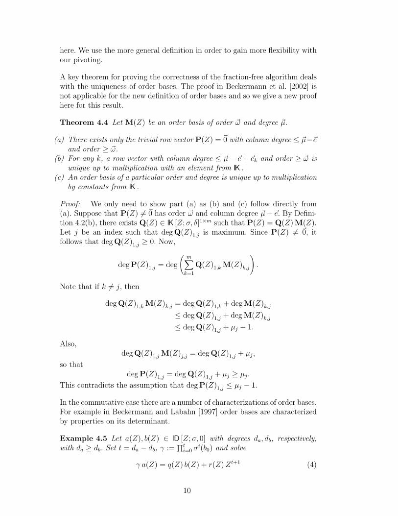
Theorem 4.4 Let M(Z) be an order basis of order ~ω and degree ~µ.
(a) There exists only the trivial row vector P(Z) = ~0 with column degree ≤ ~µ−~eand order ≥ ~ω.
(b) For any k, a row vector with column degree ≤ ~µ− ~e+ ~ek and order ≥ ~ω isunique up to multiplication with an element from IK .
(c) An order basis of a particular order and degree is unique up to multiplicationby constants from IK .
Proof: We only need to show part (a) as (b) and (c) follow directly from(a). Suppose that P(Z) 6= ~0 has order ~ω and column degree ~µ− ~e. By Defini-tion 4.2(b), there exists Q(Z) ∈ IK [Z;σ, δ]1×m such that P(Z) = Q(Z) M(Z).Let j be an index such that deg Q(Z)1,j is maximum. Since P(Z) 6= ~0, itfollows that deg Q(Z)1,j ≥ 0. Now,
deg P(Z)1,j = deg
(m∑k=1
Q(Z)1,k M(Z)k,j
).
Note that if k 6= j, then
deg Q(Z)1,k M(Z)k,j = deg Q(Z)1,k + deg M(Z)k,j≤ deg Q(Z)1,j + deg M(Z)k,j≤ deg Q(Z)1,j + µj − 1.
Also,deg Q(Z)1,j M(Z)j,j = deg Q(Z)1,j + µj,
so thatdeg P(Z)1,j = deg Q(Z)1,j + µj ≥ µj.
This contradicts the assumption that deg P(Z)1,j ≤ µj − 1.
In the commutative case there are a number of characterizations of order bases.For example in Beckermann and Labahn [1997] order bases are characterizedby properties on its determinant.
Example 4.5 Let a(Z), b(Z) ∈ ID [Z;σ, 0] with degrees da, db, respectively,with da ≥ db. Set t = da − db, γ :=
∏ti=0 σ
i(b0) and solve
γ a(Z) = q(Z) b(Z) + r(Z)Zt+1 (4)
10
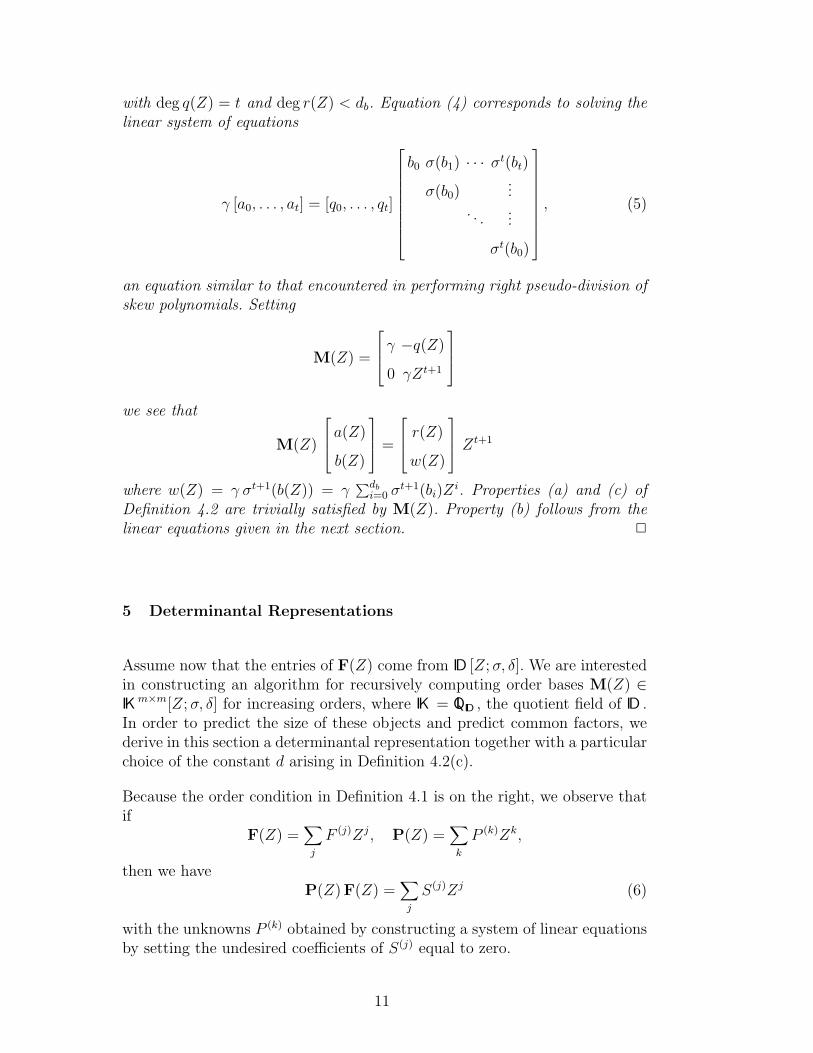
with deg q(Z) = t and deg r(Z) < db. Equation (4) corresponds to solving thelinear system of equations
γ [a0, . . . , at] = [q0, . . . , qt]
b0 σ(b1) · · · σt(bt)
σ(b0)...
. . ....
σt(b0)
, (5)
an equation similar to that encountered in performing right pseudo-division ofskew polynomials. Setting
M(Z) =
γ −q(Z)
0 γZt+1
we see that
M(Z)
a(Z)
b(Z)
=
r(Z)
w(Z)
Zt+1
where w(Z) = γ σt+1(b(Z)) = γ∑dbi=0 σ
t+1(bi)Zi. Properties (a) and (c) of
Definition 4.2 are trivially satisfied by M(Z). Property (b) follows from thelinear equations given in the next section. 2
5 Determinantal Representations
Assume now that the entries of F(Z) come from ID [Z;σ, δ]. We are interestedin constructing an algorithm for recursively computing order bases M(Z) ∈IKm×m[Z;σ, δ] for increasing orders, where IK = QID , the quotient field of ID .In order to predict the size of these objects and predict common factors, wederive in this section a determinantal representation together with a particularchoice of the constant d arising in Definition 4.2(c).
Because the order condition in Definition 4.1 is on the right, we observe thatif
F(Z) =∑j
F (j)Zj, P(Z) =∑k
P (k)Zk,
then we haveP(Z) F(Z) =
∑j
S(j)Zj (6)
with the unknowns P (k) obtained by constructing a system of linear equationsby setting the undesired coefficients of S(j) equal to zero.
11
Let us examine the underlying system of linear equations. Notice first that forany A(Z) ∈ IK [Z;σ, δ] we may write
ck(Z A(Z)) = σ(ck−1(A(Z))) + δ(ck(A(Z))) (7)
where ck denotes the kth coefficient of a polynomial (with c−1 = 0). We maywrite (7) in terms of linear algebra. Denote by C = (cu,v)u,v=0,1,... the lowertriangular infinite matrix of operators defined by cu,u = δ, cu+1,u = σ and 0otherwise, and by Cµ (µ ≥ 0) its principal submatrix of order µ. Furthermore,for each A(Z) ∈ IK [Z;σ, δ] and nonnegative integer µ we associate vectors ofcoefficients
A(µ) = [c0(A(Z)), . . . , cµ−1(A(Z))]T = [A(0), . . . , A(µ−1)]T , (8)
A = [c0(A(Z)), c1(A(Z)), . . .]T = [A(0), A(1), . . . ]T . (9)
Note that we begin our row and column enumeration at 0. We can interpret(7) in terms of matrices by
Cµ A(µ) = [c0(Z A(Z)), . . . , cµ−1(Z A(Z))]T .
Comparing with (6), we know that P(Z) has order ~ω if and only if for each` = 1, ..., s, j = 0, ..., ω` − 1 we have
m∑k=1
cj(P(Z)1,k F(Z)k,`) = 0.
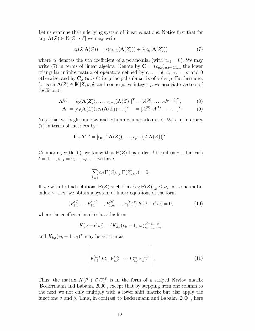
If we wish to find solutions P(Z) such that deg P(Z)1,k ≤ νk for some multi-index ~ν, then we obtain a system of linear equations of the form
(P(0)1,1 , ..., P
(ν1)1,1 , ..., P
(0)1,m, ..., P
(νm)1,m )K(~ν + ~e, ~ω) = 0, (10)
where the coefficient matrix has the form
K(~ν + ~e, ~ω) = (Kk,`(νk + 1, ω`))`=1,...,sk=1,...,m,
and Kk,`(νk + 1, ω`)T may be written asF
(ω`)k,` Cω` F
(ω`)k,` · · · Cνk
ω`F
(ω`)k,`
. (11)
Thus, the matrix K(~ν + ~e, ~ω)T is in the form of a striped Krylov matrix[Beckermann and Labahn, 2000], except that by stepping from one column tothe next we not only multiply with a lower shift matrix but also apply thefunctions σ and δ. Thus, in contrast to Beckermann and Labahn [2000], here
12
we obtain a striped Krylov matrix with a matrix C having operator-valuedelements.
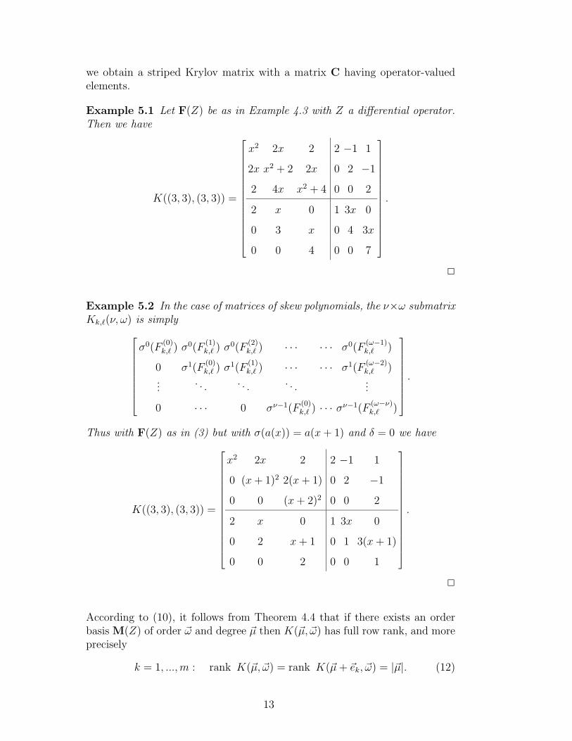
Example 5.1 Let F(Z) be as in Example 4.3 with Z a differential operator.Then we have
K((3, 3), (3, 3)) =
x2 2x 2 2 −1 1
2x x2 + 2 2x 0 2 −1
2 4x x2 + 4 0 0 2
2 x 0 1 3x 0
0 3 x 0 4 3x
0 0 4 0 0 7
.
2
Example 5.2 In the case of matrices of skew polynomials, the ν×ω submatrixKk,`(ν, ω) is simply
σ0(F(0)k,` ) σ0(F
(1)k,` ) σ0(F
(2)k,` ) · · · · · · σ0(F
(ω−1)k,` )
0 σ1(F(0)k,` ) σ1(F
(1)k,` ) · · · · · · σ1(F
(ω−2)k,` )
.... . . . . . . . .
...
0 · · · 0 σν−1(F(0)k,` ) · · · σν−1(F
(ω−ν)k,` )
.
Thus with F(Z) as in (3) but with σ(a(x)) = a(x+ 1) and δ = 0 we have
K((3, 3), (3, 3)) =
x2 2x 2 2 −1 1
0 (x+ 1)2 2(x+ 1) 0 2 −1
0 0 (x+ 2)2 0 0 2
2 x 0 1 3x 0
0 2 x+ 1 0 1 3(x+ 1)
0 0 2 0 0 1
.
2
According to (10), it follows from Theorem 4.4 that if there exists an orderbasis M(Z) of order ~ω and degree ~µ then K(~µ, ~ω) has full row rank, and moreprecisely
k = 1, ...,m : rank K(~µ, ~ω) = rank K(~µ+ ~ek, ~ω) = |~µ|. (12)
13

Suppose more generally that ~µ and ~ω are multi-indices verifying (12). Wecall a multigradient d = d(~µ, ~ω) any constant ±1 times the determinant of aregular submatrix K∗(~µ, ~ω) of maximal order of K(~µ, ~ω), and a Mahler systemcorresponding to (~µ, ~ω) a matrix of Ore polynomial M(Z) with rows havingorder ~ω and degree structure
M(z) = d · Z~µ + lower order column degrees.
In order to show that such a system exists, we state explicitly the linearsystem of equations needed to compute the unknown coefficients of the kthrow of M(Z): denote by bk(~µ, ~ω) the row added while passing from K(~µ, ~ω)to K(~µ + ~ek, ~ω). Then, by (10), the vector of coefficients is a solution of the(overdetermined) system
x ·K(~µ, ~ω) = d · bk(~µ, ~ω)
which by (12) is equivalent to the system
x ·K∗(~µ, ~ω) = d · bk∗(~µ, ~ω), (13)
where in bk∗(~µ, ~ω) and in K∗(~µ+~ek, ~ω) we keep the same columns as in K∗(~µ, ~ω).Notice that by Cramer’s rule, (13) leads to a solution with coefficients in ID .Moreover, we may formally write down a determinantal representation of theelements of a determinantal order basis, namely
M(Z)k,` = ± det[K∗(~µ+ ~ek, ~ω) E`,µ`−1+δ`,k(Z)
](14)
withE`,ν(Z) = [0, . . . , 0|1, Z, . . . , Zν |0, . . . , 0]T , (15)
the nonzero entries in E`,ν(Z) occurring in the `th stripe. In addition, we havethat
R(Z)k,` Z~ω =
∑j
M(Z)k,jF(Z)j,` = ± det[K∗(~µ+ ~ek, ~ω) E`,~µ+~ek(Z)
], (16)
where
E~ν(Z) = [F(Z)1,`, . . . , Zν1−1F(Z)1,`| . . . . . . |F(Z)m,`, . . . , Z
νm−1F(Z)m,`]T .
In both (14) and (16) the matrices have commutative entries in all but thelast column. It is understood that the determinant in both cases is expandedalong this column.
Finally we mention that, by the uniqueness result of Theorem 4.4, any orderbasis of degree ~µ and order ~ω coincides up to multiplication with some elementin IK with an Mahler system associated to (~µ, ~ω), which therefore itself is anorder basis of the same degree and order. By a particular pivoting techniquewe get a reduced order basis by computing Mahler systems.
14
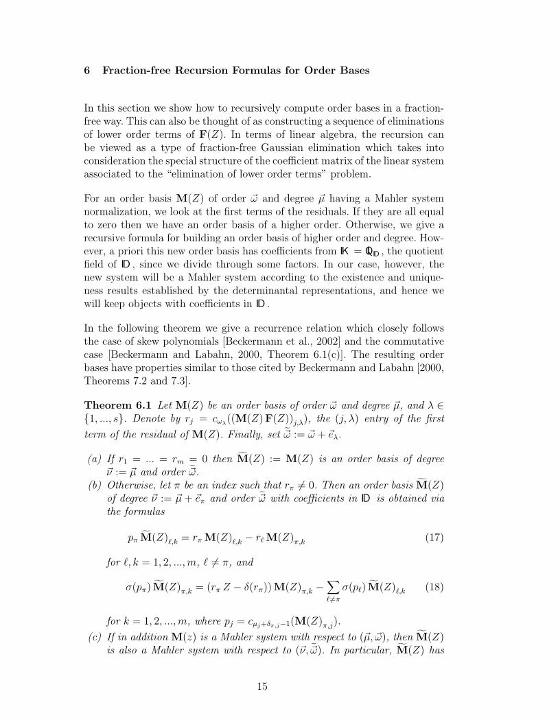
6 Fraction-free Recursion Formulas for Order Bases
In this section we show how to recursively compute order bases in a fraction-free way. This can also be thought of as constructing a sequence of eliminationsof lower order terms of F(Z). In terms of linear algebra, the recursion canbe viewed as a type of fraction-free Gaussian elimination which takes intoconsideration the special structure of the coefficient matrix of the linear systemassociated to the “elimination of lower order terms” problem.
For an order basis M(Z) of order ~ω and degree ~µ having a Mahler systemnormalization, we look at the first terms of the residuals. If they are all equalto zero then we have an order basis of a higher order. Otherwise, we give arecursive formula for building an order basis of higher order and degree. How-ever, a priori this new order basis has coefficients from IK = QID , the quotientfield of ID , since we divide through some factors. In our case, however, thenew system will be a Mahler system according to the existence and unique-ness results established by the determinantal representations, and hence wewill keep objects with coefficients in ID .
In the following theorem we give a recurrence relation which closely followsthe case of skew polynomials [Beckermann et al., 2002] and the commutativecase [Beckermann and Labahn, 2000, Theorem 6.1(c)]. The resulting orderbases have properties similar to those cited by Beckermann and Labahn [2000,Theorems 7.2 and 7.3].
Theorem 6.1 Let M(Z) be an order basis of order ~ω and degree ~µ, and λ ∈{1, ..., s}. Denote by rj = cωλ((M(Z) F(Z))j,λ), the (j, λ) entry of the first
term of the residual of M(Z). Finally, set ~ω := ~ω + ~eλ.
(a) If r1 = ... = rm = 0 then M(Z) := M(Z) is an order basis of degree~ν := ~µ and order ~ω.
(b) Otherwise, let π be an index such that rπ 6= 0. Then an order basis M(Z)of degree ~ν := ~µ + ~eπ and order ~ω with coefficients in ID is obtained viathe formulas
pπ M(Z)`,k = rπ M(Z)`,k − r` M(Z)π,k (17)
for `, k = 1, 2, ...,m, ` 6= π, and
σ(pπ) M(Z)π,k = (rπ Z − δ(rπ)) M(Z)π,k −∑` 6=π
σ(p`) M(Z)`,k (18)
for k = 1, 2, ...,m, where pj = cµj+δπ,j−1(M(Z)π,j).
(c) If in addition M(z) is a Mahler system with respect to (~µ, ~ω), then M(Z)is also a Mahler system with respect to (~ν, ~ω). In particular, M(Z) has
15
coefficients in ID .
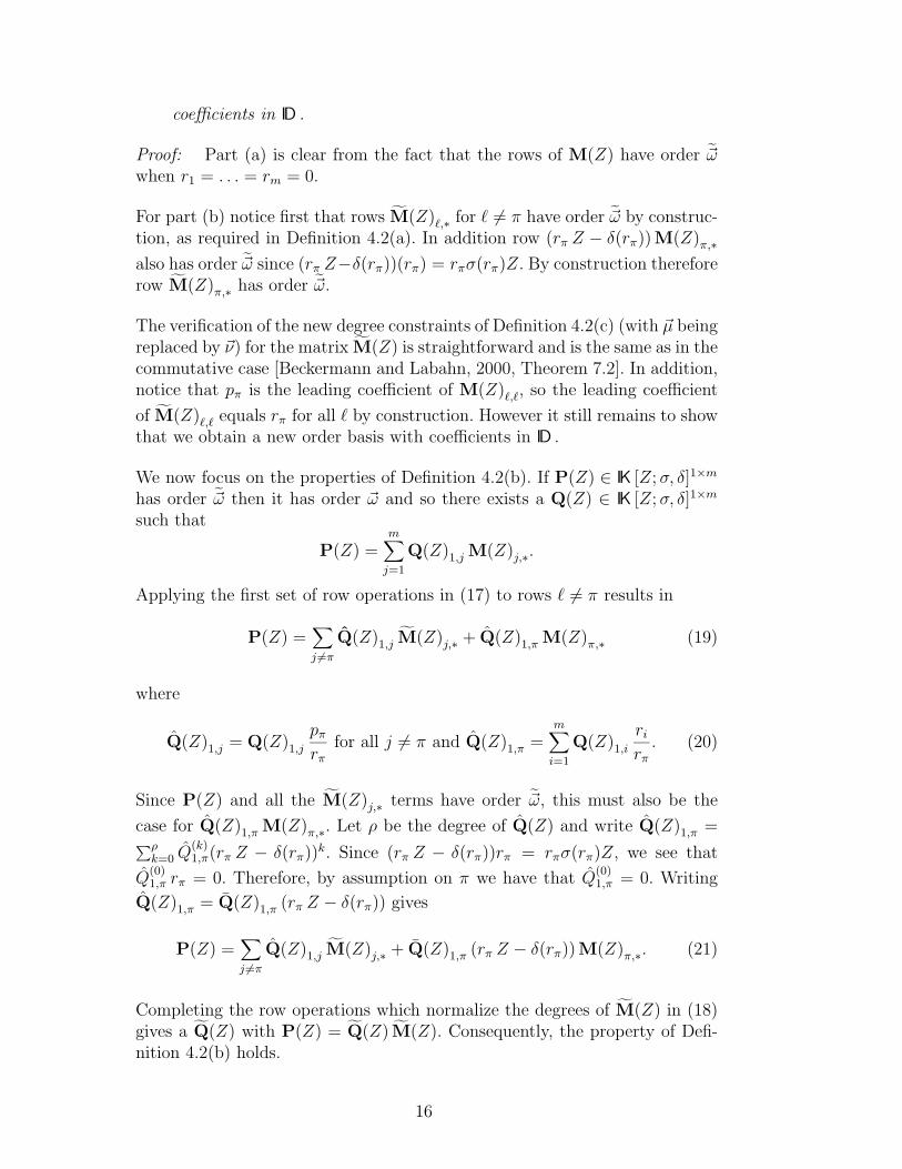
Proof: Part (a) is clear from the fact that the rows of M(Z) have order ~ωwhen r1 = . . . = rm = 0.
For part (b) notice first that rows M(Z)`,∗ for ` 6= π have order ~ω by construc-tion, as required in Definition 4.2(a). In addition row (rπ Z − δ(rπ)) M(Z)π,∗also has order ~ω since (rπ Z−δ(rπ))(rπ) = rπσ(rπ)Z. By construction thereforerow M(Z)π,∗ has order ~ω.
The verification of the new degree constraints of Definition 4.2(c) (with ~µ beingreplaced by ~ν) for the matrix M(Z) is straightforward and is the same as in thecommutative case [Beckermann and Labahn, 2000, Theorem 7.2]. In addition,notice that pπ is the leading coefficient of M(Z)`,`, so the leading coefficient
of M(Z)`,` equals rπ for all ` by construction. However it still remains to showthat we obtain a new order basis with coefficients in ID .
We now focus on the properties of Definition 4.2(b). If P(Z) ∈ IK [Z;σ, δ]1×m
has order ~ω then it has order ~ω and so there exists a Q(Z) ∈ IK [Z;σ, δ]1×m
such that
P(Z) =m∑j=1
Q(Z)1,j M(Z)j,∗.
Applying the first set of row operations in (17) to rows ` 6= π results in
P(Z) =∑j 6=π
Q(Z)1,j M(Z)j,∗ + Q(Z)1,π M(Z)π,∗ (19)
where
Q(Z)1,j = Q(Z)1,j
pπrπ
for all j 6= π and Q(Z)1,π =m∑i=1
Q(Z)1,i
rirπ. (20)
Since P(Z) and all the M(Z)j,∗ terms have order ~ω, this must also be the
case for Q(Z)1,π M(Z)π,∗. Let ρ be the degree of Q(Z) and write Q(Z)1,π =∑ρk=0 Q
(k)1,π(rπ Z − δ(rπ))k. Since (rπ Z − δ(rπ))rπ = rπσ(rπ)Z, we see that
Q(0)1,π rπ = 0. Therefore, by assumption on π we have that Q
(0)1,π = 0. Writing
Q(Z)1,π = Q(Z)1,π (rπ Z − δ(rπ)) gives
P(Z) =∑j 6=π
Q(Z)1,j M(Z)j,∗ + Q(Z)1,π (rπ Z − δ(rπ)) M(Z)π,∗. (21)
Completing the row operations which normalize the degrees of M(Z) in (18)gives a Q(Z) with P(Z) = Q(Z) M(Z). Consequently, the property of Defi-nition 4.2(b) holds.
16
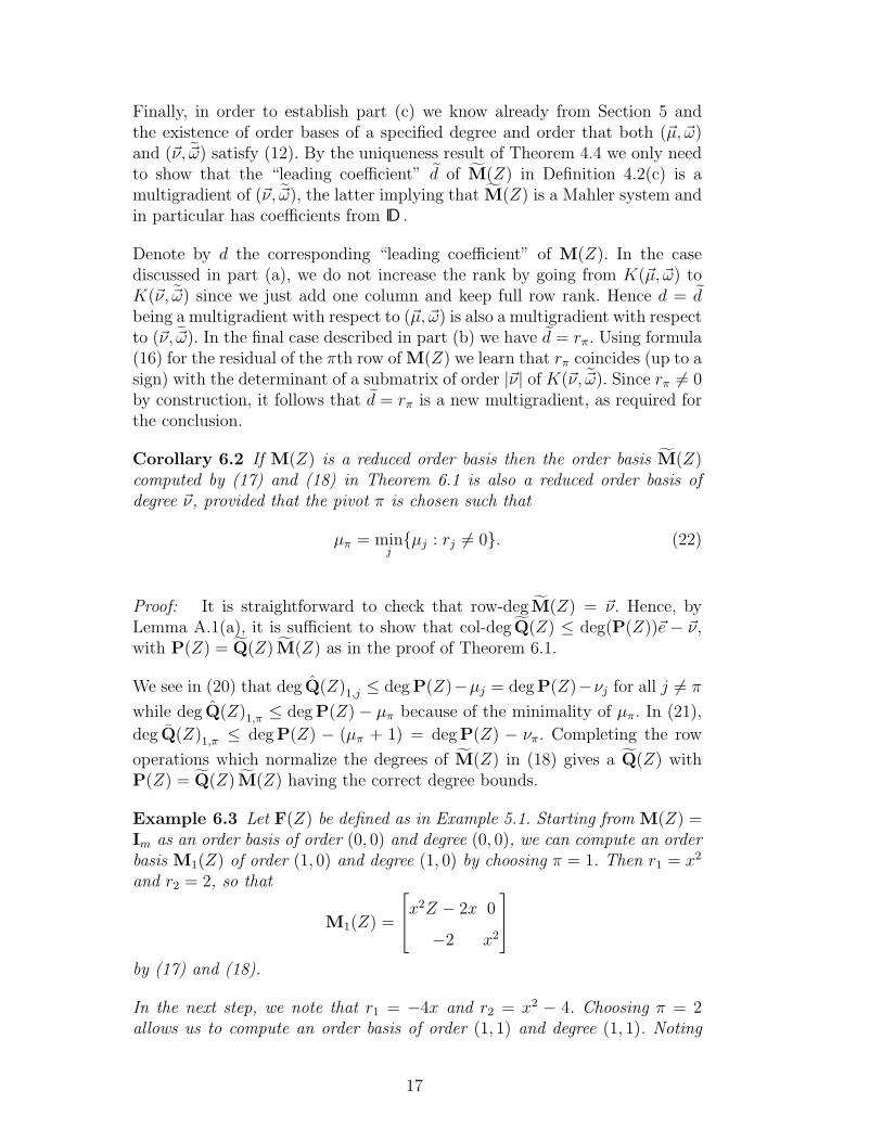
Finally, in order to establish part (c) we know already from Section 5 andthe existence of order bases of a specified degree and order that both (~µ, ~ω)and (~ν, ~ω) satisfy (12). By the uniqueness result of Theorem 4.4 we only needto show that the “leading coefficient” d of M(Z) in Definition 4.2(c) is amultigradient of (~ν, ~ω), the latter implying that M(Z) is a Mahler system andin particular has coefficients from ID .
Denote by d the corresponding “leading coefficient” of M(Z). In the casediscussed in part (a), we do not increase the rank by going from K(~µ, ~ω) toK(~ν, ~ω) since we just add one column and keep full row rank. Hence d = dbeing a multigradient with respect to (~µ, ~ω) is also a multigradient with respectto (~ν, ~ω). In the final case described in part (b) we have d = rπ. Using formula(16) for the residual of the πth row of M(Z) we learn that rπ coincides (up to asign) with the determinant of a submatrix of order |~ν| of K(~ν, ~ω). Since rπ 6= 0by construction, it follows that d = rπ is a new multigradient, as required forthe conclusion.
Corollary 6.2 If M(Z) is a reduced order basis then the order basis M(Z)computed by (17) and (18) in Theorem 6.1 is also a reduced order basis ofdegree ~ν, provided that the pivot π is chosen such that
µπ = minj{µj : rj 6= 0}. (22)
Proof: It is straightforward to check that row-deg M(Z) = ~ν. Hence, byLemma A.1(a), it is sufficient to show that col-deg Q(Z) ≤ deg(P(Z))~e − ~ν,with P(Z) = Q(Z) M(Z) as in the proof of Theorem 6.1.
We see in (20) that deg Q(Z)1,j ≤ deg P(Z)−µj = deg P(Z)−νj for all j 6= π
while deg Q(Z)1,π ≤ deg P(Z)− µπ because of the minimality of µπ. In (21),
deg Q(Z)1,π ≤ deg P(Z) − (µπ + 1) = deg P(Z) − νπ. Completing the row
operations which normalize the degrees of M(Z) in (18) gives a Q(Z) withP(Z) = Q(Z) M(Z) having the correct degree bounds.
Example 6.3 Let F(Z) be defined as in Example 5.1. Starting from M(Z) =Im as an order basis of order (0, 0) and degree (0, 0), we can compute an orderbasis M1(Z) of order (1, 0) and degree (1, 0) by choosing π = 1. Then r1 = x2
and r2 = 2, so that
M1(Z) =
x2Z − 2x 0
−2 x2
by (17) and (18).
In the next step, we note that r1 = −4x and r2 = x2 − 4. Choosing π = 2allows us to compute an order basis of order (1, 1) and degree (1, 1). Noting
17
that the previous pivot x2 is a common factor, (17) and (18) gives the orderbasis M(Z) found in Example 4.3. 2
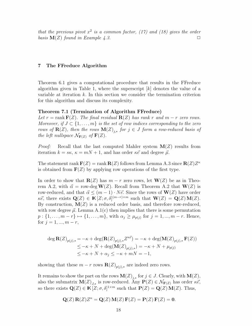
7 The FFreduce Algorithm
Theorem 6.1 gives a computational procedure that results in the FFreducealgorithm given in Table 1, where the superscript [k] denotes the value of avariable at iteration k. In this section we consider the termination criterionfor this algorithm and discuss its complexity.
Theorem 7.1 (Termination of Algorithm FFreduce)Let r = rank F(Z). The final residual R(Z) has rank r and m− r zero rows.Moreover, if J ⊂ {1, . . . ,m} is the set of row indices corresponding to the zerorows of R(Z), then the rows M(Z)j,∗ for j ∈ J form a row-reduced basis ofthe left nullspace NF(Z) of F(Z).
Proof: Recall that the last computed Mahler system M(Z) results fromiteration k = sκ, κ = mN + 1, and has order κ~e and degree ~µ.
The statement rank F(Z) = rank R(Z) follows from Lemma A.3 since R(Z)Zκ
is obtained from F(Z) by applying row operations of the first type.
In order to show that R(Z) has m − r zero rows, let W(Z) be as in Theo-rem A.2, with ~α = row-deg W(Z). Recall from Theorem A.2 that W(Z) isrow-reduced, and that ~α ≤ (m− 1) ·N~e. Since the rows of W(Z) have orderκ~e, there exists Q(Z) ∈ IK [Z;σ, δ](m−r)×m such that W(Z) = Q(Z) M(Z).By construction, M(Z) is a reduced order basis, and therefore row-reduced,with row degree ~µ. Lemma A.1(c) then implies that there is some permutationp : {1, . . . ,m − r} 7→ {1, . . . ,m}, with αj ≥ µp(j) for j = 1, ...,m − r. Hence,for j = 1, ...,m− r,
deg R(Z)p(j),∗=−κ+ deg(R(Z)p(j),∗Zκ~e) = −κ+ deg(M(Z)p(j),∗F(Z))
≤−κ+N + deg(M(Z)p(j),∗) = −κ+N + µp(j)
≤−κ+N + αj ≤ −κ+mN = −1,
showing that these m− r rows R(Z)p(j),∗ are indeed zero rows.
It remains to show the part on the rows M(Z)j,∗ for j ∈ J . Clearly, with M(Z),also the submatrix M(Z)J,∗ is row-reduced. Any P(Z) ∈ NF(Z) has order κ~e,
so there exists Q(Z) ∈ IK [Z;σ, δ]1×m such that P(Z) = Q(Z) M(Z). Thus,
Q(Z) R(Z)Zκ = Q(Z) M(Z) F(Z) = P(Z) F(Z) = 0.
18
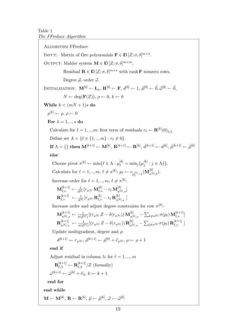
Table 1The FFreduce Algorithm
Algorithm FFreduce
Input: Matrix of Ore polynomials F ∈ ID [Z;σ, δ]m×s.
Output: Mahler system M ∈ ID [Z;σ, δ]m×m,
Residual R ∈ ID [Z;σ, δ]m×s with rank F nonzero rows,
Degree ~µ, order ~ω.
Initialization: M[0] ← Im, R[0] ← F, d[0] ← 1, ~µ[0] ← ~0, ~ω[0] ← ~0,
N ← deg(F(Z)), ρ← 0, k ← 0
While k < (mN + 1)s do
ρ[k] ← ρ, ρ← 0
For λ = 1, .., s do
Calculate for ` = 1, ..,m: first term of residuals r` ← R[k](0)`,λ
Define set Λ = {` ∈ {1, ..,m} : r` 6= 0}.
If Λ = {} then M[k+1] ←M[k], R[k+1] ← R[k], d[k+1] ← d[k], ~µ[k+1] ← ~µ[k]
else
Choose pivot π[k] ← min{` ∈ Λ : µ[k]` = minj{µ[k]
j : j ∈ Λ}}.
Calculate for ` = 1, ..,m, ` 6= π[k]: p` ← cµ
[k]`−1
(M[k]
π[k],`).
Increase order for ` = 1, ..,m, ` 6= π[k]:
M[k+1]`,∗ ← 1
d[k] [rπ[k] M[k]`,∗ − r` M[k]
π[k],∗]
R[k+1]`,∗ ← 1
d[k] [rπ[k] R[k]`,∗ − r` R[k]
π[k],∗ ]
Increase order and adjust degree constraints for row π[k]:
M[k+1]
π[k],∗ ←1
σ(d[k])[(rπ[k] Z − δ(rπ[k])) M[k]
π[k],∗ −∑
` 6=π[k] σ(p`) M[k+1]`,∗ ]
R[k+1]
π[k],∗ ←1
σ(d[k])[(rπ[k] Z − δ(rπ[k])) R[k]
π[k],∗ −∑
` 6=π[k] σ(p`) R[k+1]`,∗ ]
Update multigradient, degree and ρ:
d[k+1] ← rπ[k] , ~µ[k+1] ← ~µ[k] + ~eπ[k] , ρ← ρ+ 1
end if
Adjust residual in column λ: for ` = 1, ...,m
R[k+1]`,λ ← R[k+1]
`,λ /Z (formally)
~ω[k+1] ← ~ω[k] + ~eλ, k ← k + 1
end for
end while
M←M[k], R← R[k], ~µ← ~µ[k], ~ω ← ~ω[k]
19
The relation r = rank R(Z) implies that the nonzero rows of R(Z) areQID [Z;σ, δ]-linearly independent, and hence Q(Z)1,j = 0 for j 6∈ J . Conse-quently, the rows of M(Z)J,∗ form a basis ofNF(Z), as claimed in Theorem 7.1.
In what follows we denote by cycle the set of iterations k = κs, κs+ 1, ..., (κ+1)s−1 in algorithm FFreduce for some integer κ (that is, the execution of theinner loop).
Let us comment on possible improvements of our termination criterion. In allexamples given in the remainder of this section, we choose as ID the set ofpolynomials in x with rational coefficients, with Z = d
dx, and thus σ(a(x)) =
a(x), δ(a(x)) = ddxa(x).
Remark 7.2 The above proof was based on the estimate αj ≤ (m − 1)N forthe left minimal indices of the left nullspace NF(Z), which for general matrixpolynomials is quite pessimistic, but can be attained, as shown in [Beckermannet al., 2001, Example 5.6] for ordinary matrix polynomials. For applicationswhere a lower bound γ is available for |~ν|, the sum of the row degrees of thenontrivial rows of the row-reduced counterpart of F(Z) (compare with The-orem 2.2), it would be sufficient to compute Mahler systems up to the finalorder (mN + 1− γ)~e, since then we get from Theorem 2.2 and Theorem A.2the improved estimate αj ≤ (m− 1)N − γ.
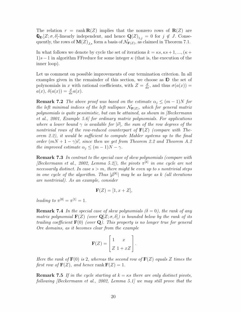
Remark 7.3 In contrast to the special case of skew polynomials (compare with[Beckermann et al., 2002, Lemma 5.2]), the pivots π[k] in one cycle are notnecessarily distinct. In case s > m, there might be even up to s nontrivial stepsin one cycle of the algorithm. Thus |~µ[k]| may be as large as k (all iterationsare nontrivial). As an example, consider
F(Z) = [1, x+ Z],
leading to π[0] = π[1] = 1.
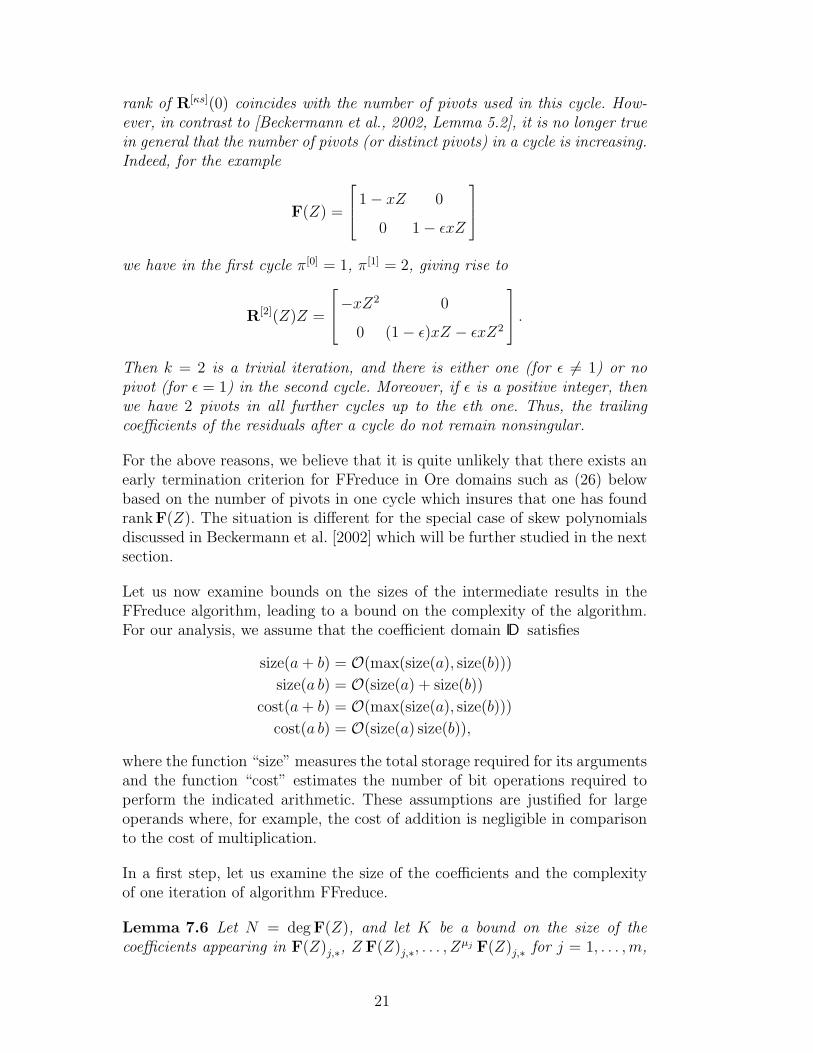
Remark 7.4 In the special case of skew polynomials (δ = 0), the rank of anymatrix polynomial F(Z) (over Q[Z;σ, δ]) is bounded below by the rank of itstrailing coefficient F(0) (over Q). This property is no longer true for generalOre domains, as it becomes clear from the example
F(Z) =
1 x
Z 1 + xZ
.Here the rank of F(0) is 2, whereas the second row of F(Z) equals Z times thefirst row of F(Z), and hence rank F(Z) = 1.
Remark 7.5 If in the cycle starting at k = κs there are only distinct pivots,following [Beckermann et al., 2002, Lemma 5.1] we may still prove that the
20
rank of R[κs](0) coincides with the number of pivots used in this cycle. How-ever, in contrast to [Beckermann et al., 2002, Lemma 5.2], it is no longer truein general that the number of pivots (or distinct pivots) in a cycle is increasing.Indeed, for the example
F(Z) =
1− xZ 0
0 1− εxZ
we have in the first cycle π[0] = 1, π[1] = 2, giving rise to
R[2](Z)Z =
−xZ2 0
0 (1− ε)xZ − εxZ2
.Then k = 2 is a trivial iteration, and there is either one (for ε 6= 1) or nopivot (for ε = 1) in the second cycle. Moreover, if ε is a positive integer, thenwe have 2 pivots in all further cycles up to the εth one. Thus, the trailingcoefficients of the residuals after a cycle do not remain nonsingular.
For the above reasons, we believe that it is quite unlikely that there exists anearly termination criterion for FFreduce in Ore domains such as (26) belowbased on the number of pivots in one cycle which insures that one has foundrank F(Z). The situation is different for the special case of skew polynomialsdiscussed in Beckermann et al. [2002] which will be further studied in the nextsection.
Let us now examine bounds on the sizes of the intermediate results in theFFreduce algorithm, leading to a bound on the complexity of the algorithm.For our analysis, we assume that the coefficient domain ID satisfies
size(a+ b) = O(max(size(a), size(b)))
size(a b) = O(size(a) + size(b))
cost(a+ b) = O(max(size(a), size(b)))
cost(a b) = O(size(a) size(b)),
where the function “size” measures the total storage required for its argumentsand the function “cost” estimates the number of bit operations required toperform the indicated arithmetic. These assumptions are justified for largeoperands where, for example, the cost of addition is negligible in comparisonto the cost of multiplication.
In a first step, let us examine the size of the coefficients and the complexityof one iteration of algorithm FFreduce.
Lemma 7.6 Let N = deg F(Z), and let K be a bound on the size of thecoefficients appearing in F(Z)j,∗, Z F(Z)j,∗, . . . , Z
µj F(Z)j,∗ for j = 1, . . . ,m,
21
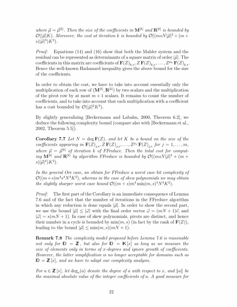
where ~µ = ~µ[k]. Then the size of the coefficients in M[k] and R[k] is bounded byO(|~µ|K). Moreover, the cost at iteration k is bounded by O((msN |~µ|2 + (m+s)|~µ|3)K2).
Proof: Equations (14) and (16) show that both the Mahler system and theresidual can be represented as determinants of a square matrix of order |~µ|. Thecoefficients in this matrix are coefficients of F(Z)k,∗, Z F(Z)k,∗, . . . , Z
µk F(Z)k,∗.Hence the well-known Hadamard inequality gives the above bound for the sizeof the coefficients.
In order to obtain the cost, we have to take into account essentially only themultiplication of each row of (M[k],R[k]) by two scalars and the multiplicationof the pivot row by at most m+ 1 scalars. It remains to count the number ofcoefficients, and to take into account that each multiplication with a coefficienthas a cost bounded by O(|~µ|2K2).
By slightly generalizing [Beckermann and Labahn, 2000, Theorem 6.2], wededuce the following complexity bound (compare also with [Beckermann et al.,2002, Theorem 5.5]).
Corollary 7.7 Let N = deg F(Z), and let K be a bound on the size of thecoefficients appearing in F(Z)j,∗, Z F(Z)j,∗, . . . , Z
µj F(Z)j,∗ for j = 1, . . . ,m,
where ~µ = ~µ[k] of iteration k of FFreduce. Then the total cost for comput-ing M[k] and R[k] by algorithm FFreduce is bounded by O((msN |~µ|3 + (m +s)|~µ|4)K2).
In the general Ore case, we obtain for FFreduce a worst case bit complexity ofO((m+s)m4s4N4K2), whereas in the case of skew polynomials we may obtainthe slightly sharper worst case bound O((m+ s)m4 min(m, s)4N4K2).
Proof: The first part of the Corollary is an immediate consequence of Lemma7.6 and of the fact that the number of iterations in the FFreduce algorithmin which any reduction is done equals |~µ|. In order to show the second part,we use the bound |~µ| ≤ |~ω| with the final order vector ~ω = (mN + 1)~e, and|~ω| = s(mN + 1). In case of skew polynomials, pivots are distinct, and hencetheir number in a cycle is bounded by min(m, s) (in fact by the rank of F(Z)),leading to the bound |~µ| ≤ min(m, s)(mN + 1).
Remark 7.8 The complexity model proposed before Lemma 7.6 is reasonablenot only for ID = ZZ , but also for ID = IK [x] as long as we measure thesize of elements only in terms of x-degrees and ignore growth of coefficients.However, the latter simplification is no longer acceptable for domains such asID = ZZ [x], and we have to adapt our complexity analysis.
For a ∈ ZZ [x], let degx(a) denote the degree of a with respect to x, and ‖a‖ bethe maximal absolute value of the integer coefficients of a. A good measure for
22
size for a nonzero a ∈ ZZ [x] seems to be
size(a) = O((1 + degx(a))(1 + log ‖a‖)),
since it reflects worst case memory requirements. In addition the two rules
cost(a+ b) = O(max(size(a), size(b)))
cost(a b) = O(size(a) size(b)).
continue to hold. However, it is easy to construct polynomials where the rulesfor size(a+ b) and size(ab) given before Lemma 7.6 are no longer true becauseof cross products between degrees and the bit lengths of the coefficients. Theessential ingredient in the proof of Lemma 7.6 (and thus of Corollary 7.7) wasto predict the size of a coefficient c[k] ∈ ZZ [x] in M[k] or in R[k], by means ofits determinant representation in terms of a matrix of order |~µ[k]| containingsuitable coefficients of ZjF(Z) for suitable j. Here we propose to estimateseparately the x-degree and the norm of c[k]. In our three examples below theapplications σ, δ : ZZ [x] 7→ ZZ [x] will not increase the degree, and thus oneeasily checks that
degx c[k] ≤ |~µ[k]|Kdeg,
with Kdeg being the maximal degree of a coefficient occurring in F(Z). Definealso Kbit to be the logarithm of the largest norm of a coefficient occurring inF(Z). We will show below that the logarithm of the norm of an entry of theabove-mentioned matrix is bounded for our three examples by
Kbit + (max`µ
[k]` ) f(Kdeg) (23)
for a suitable function f depending only on σ, δ, and hence
size(c[k]) = O((1 + |~µ[k]|Kdeg)(1 + |~µ[k]|Kbit + |~µ[k]| (max`µ
[k]` ) f(Kdeg)))
orsize(c[k]) = O(KdegKbit|~µ[k]|2 +Kdegf(Kdeg)|~µ[k]|3),
in contrast to size(c[k]) = O(K|~µ[k]|) derived in Lemma 7.6. As a consequence,we may directly generalize both Lemma 7.6 and Corollary 7.7, but now higherpowers will be involved. Notice that a tighter estimate could be obtained if wespecify the size and cost of the sums and products in two components (degx(a)and ‖a‖) separately [Li, 2003].
Let us first consider the skew-symmetric case σ(a(x)) = a(αx), δ(a) = 0,for an integer α 6= 0. Since for the norm of the coefficients of Zkxj weget log(||σk(xj)||) = j k log(|α|), we observe that (23) holds with f(Kdeg) =Kdeg log(|α|).
More generally, for the skew-symmetric case σ(a(x)) = a(αx + β), δ(a) = 0with integers α 6= 0 and β, we have log(||σk(xj)||) ≤ j k log(2 max(|α|, |β|)).Thus here (23) holds with f(Kdeg) = Kdeg log(2 max(|α|, |β|)).
23
We finally consider the differential case in which σ is the identity and δ(a) =ddxa for all a ∈ ZZ [x]. Then σ does not increase the norm, and ||δ(a)|| ≤
degx(a) ||a||, implying that (23) holds with f(Kdeg) = log(Kdeg).
8 Comparisons and Examples
In this section we give some examples which allow us to make some simplecomparisons with the algorithm in Abramov and Bronstein [2001]. We makeno claims that our algorithm performs better than theirs in general. Indeedfor examples where coefficient growth does not enter into the problem, thealgorithm of Abramov and Bronstein is typically faster than the one presentedin this paper. However, there are instances where the growth of coefficientsdoes become a significant factor and in such cases the near linear growth ofour algorithm does allow us to solve larger problems.
The Abramov-Bronstein algorithm uses the constructive approach outlined inTheorem 2.2. It also incorporates a number of additional improvements, forexample making use of a basis of elements from the nullspace of the lead-ing or trailing coefficients (rather than just a single element) in order to re-duce the number of iterations [Abramov and Bronstein, 2002]. We also notethat since the row-reduced form is not unique, the results computed by theAbramov-Bronstein algorithm are typically different from the ones obtainedby FFreduce.
It is possible, as suggested in Abramov and Bronstein [2001], to computethe basis for the nullspace by using fraction-free Gaussian elimination on theleading or trailing coefficient matrix, see Bareiss [1968]. This also results in afraction-free algorithm for row-reducing a matrix of skew polynomials. How-ever it is not the case that this guarantees a reasonable growth of coefficientsize. For example, one step of such a method could result in an increased sizeof coefficients by a factor of r + 1 where r is the rank of the actual trailingor leading coefficient matrix. This occurs because the nullspace obtained byBareiss’s method could be as large as r times the original input size. Evenremoving the contents of the nullspace elements afterwards will not guaranteegood coefficient growth as our examples below illustrate.
The implementation of the Abramov-Bronstein algorithm used for our com-parisons is that programmed in Maple given in the routine LinearFunction-alSystems[MatrixTriangularization]. This implementation finds a basis for thenullspace by working over a field and then clearing denominators. Notice thatthis approach is mathematically equivalent to using fraction-free Gaussianelimination and then removing the contents from individual basis elements.Note that the contents are only removed from the basis elements used to per-
24
form the elimination. The contents in the intermediate results are not removed,so that exponential growth may still occur. This implementation performs ad-ditional optimizations when the trailing coefficient has a zero row or a zerocolumn. This reduces the number of iterations required to obtain the finalresult. Our fraction-free algorithm can be adopted to perform such shifts aswell. In our comparison, such optimizations are performed in the Abramov-Bronstein algorithm but not in the fraction-free one. Finally, we have done aslight modification to ensure that it works in the case when the rank is notfull.
We have run several examples, including those of [Abramov and Bronstein,2002], in which the dimensions of the matrices, as well as the degree, arevaried. For the measure of size we have used the sum of Maple’s length of allthe coefficients over Q[n], namely the coefficients of the residuals for the ABalgorithm and the coefficients of both the Mahler system and the residuals forFFreduce.
For examples in which coefficient growth is not significant, the Abramov-Bronstein algorithm is in general faster, sometimes by more than a factor of1000. For these examples, the cost of GCD computations required for removingthe content (or for clearing fractions) was negligible.
In contrast, consider the matrix
F(Z) =
∑Ni=0 piZ
i ∑N−1i=0 piZ
i∑Ni=0 pi+N+1Z
i ∑N−1i=0 pi+N+1Z
i
(24)
where pi is the (i+1)-th prime and where we are working over the commutativepolynomial domain Z[Z]. The storage and running time requirements for thismatrix using the two algorithms is given in Figure 1. In particular we seethat the growth in the Abramov-Bronstein algorithm is exponential (varyingbetween 48 for N = 5 and 58685030 for N = 300) while that of FFreduce isessentially linear for this case (varying between 97 and 880154). This of courseimpacts the timings of the two algorithms for this example.
Similarly such growth is also possible in the noncommutative case of skewpolynomials. For example, one can construct matrices similar to that of (24)but using a noncommutative Z and get comparable behaviour. This is thecase with
F(Z) =
q0,N(Z) q0,N−1(Z) q0,N−2(Z)
q2N+2,N(Z) q2N+2,N−1(Z) q4N+4,N−2(Z)
q4N+4,N(Z) q4N+4,N−1(Z) q2N+2,N−2(Z)
(25)
25
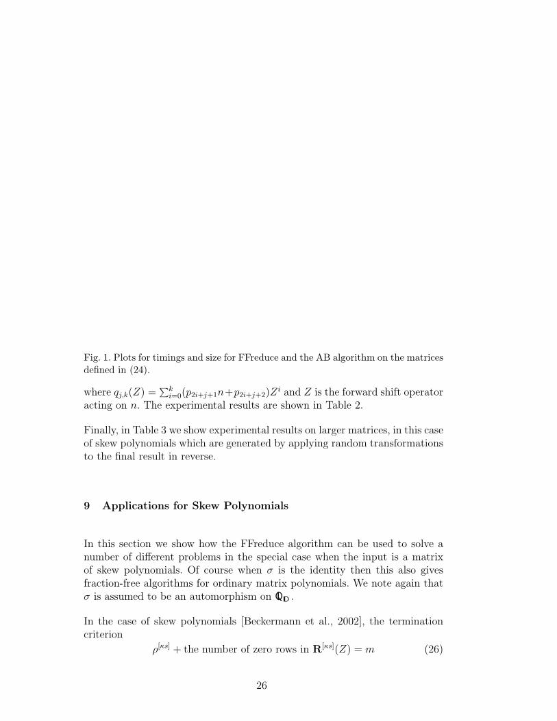
Fig. 1. Plots for timings and size for FFreduce and the AB algorithm on the matricesdefined in (24).
where qj,k(Z) =∑ki=0(p2i+j+1n+p2i+j+2)Zi and Z is the forward shift operator
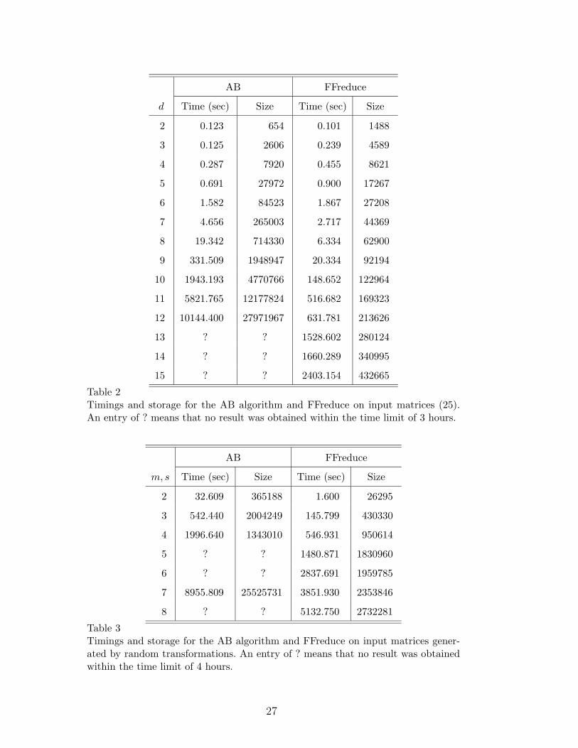
acting on n. The experimental results are shown in Table 2.
Finally, in Table 3 we show experimental results on larger matrices, in this caseof skew polynomials which are generated by applying random transformationsto the final result in reverse.
9 Applications for Skew Polynomials
In this section we show how the FFreduce algorithm can be used to solve anumber of different problems in the special case when the input is a matrixof skew polynomials. Of course when σ is the identity then this also givesfraction-free algorithms for ordinary matrix polynomials. We note again thatσ is assumed to be an automorphism on QID .
In the case of skew polynomials [Beckermann et al., 2002], the terminationcriterion
ρ[κs] + the number of zero rows in R[κs](Z) = m (26)
26
AB FFreduce
d Time (sec) Size Time (sec) Size
2 0.123 654 0.101 1488
3 0.125 2606 0.239 4589
4 0.287 7920 0.455 8621
5 0.691 27972 0.900 17267
6 1.582 84523 1.867 27208
7 4.656 265003 2.717 44369
8 19.342 714330 6.334 62900
9 331.509 1948947 20.334 92194
10 1943.193 4770766 148.652 122964
11 5821.765 12177824 516.682 169323
12 10144.400 27971967 631.781 213626
13 ? ? 1528.602 280124
14 ? ? 1660.289 340995
15 ? ? 2403.154 432665
Table 2Timings and storage for the AB algorithm and FFreduce on input matrices (25).An entry of ? means that no result was obtained within the time limit of 3 hours.
AB FFreduce
m, s Time (sec) Size Time (sec) Size
2 32.609 365188 1.600 26295
3 542.440 2004249 145.799 430330
4 1996.640 1343010 546.931 950614
5 ? ? 1480.871 1830960
6 ? ? 2837.691 1959785
7 8955.809 25525731 3851.930 2353846
8 ? ? 5132.750 2732281
Table 3Timings and storage for the AB algorithm and FFreduce on input matrices gener-ated by random transformations. An entry of ? means that no result was obtainedwithin the time limit of 4 hours.
27
allows us to prove [Beckermann et al., 2002, Theorem 5.3] that
rank R[κs](0) = rank R[κs](Z)) = rank F(Z), (27)
the rank of the trailing coefficient matrix R[κs](0) being defined over the quo-tient field QID . Moreover [Beckermann et al., 2002, Lemma 5.2],
the pivots π[k] for κs− s ≤ k < κs are distinct, (28)
and hence [Beckermann et al., 2002, Lemma 5.1 and Lemma 5.2]
ρ[κs] = rank R[κs](0) = rank R[κs−s](0). (29)
It is also shown implicitly in the proof of [Beckermann et al., 2002, Theo-rem 5.4] that κ ≤ m(N + 1) which has to be compared with the number ofcycles, mN + 1, required by FFreduce. Thus the new termination property(26) essentially does not increase the complexity of algorithm FFreduce, butfor many examples may improve the run time.
9.1 Full Rank Decomposition and Solutions of Linear Functional Systems
When F(Z) represents a system of linear recurrence equations, one can showthat an equivalent system with a leading (or trailing) coefficient with full rowrank allows one to obtain bounds on the degrees of the numerator and thedenominator of all rational solutions. This has been used by Abramov andBronstein [2001] to compute rational solutions of linear functional systems.
In [Beckermann et al., 2002] it is shown that the output of FFreduce applied toF(Z) ∈ ID [Z;σ, 0]m×s can be used to construct T(Z−1) ∈ ID [Z−1;σ−1, 0]m×m
and implicitly S(Z) ∈ QID [Z;σ, 0]m×m such that
T(Z−1) F(Z) = W(Z) ∈ ID [Z;σ, 0]m×s, S(Z)T(Z−1) = Im,
with the number of nonzero rows of W(Z) coinciding with the rank of thetrailing coefficient W(0), and hence with the rank of W(Z). The existence ofa left inverse S(Z) shows that the reduction process is invertible in the algebraof Laurent skew polynomials, moreover, we obtain a full rank decompositionF(Z) = S(Z)W(Z) in QID [Z;σ, 0].
In this context we should mention that an exact arithmetic method involvingcoefficient GCD computations for the computation of T(Z−1) F(Z) = W(Z)with W(Z) as above has already been given in Abramov and Bronstein [2001].
28
9.2 Row-reduced Form and Weak Popov Form
The FFreduce algorithm as described above has been used to eliminate low-order coefficients, such that the rank of the trailing coefficient matrix is thesame as the rank of the original matrix of skew polynomials. In the case ofmatrices of commutative polynomials, we can reverse the coefficients so thatthe high-order coefficients are eliminated [Beckermann and Labahn, 2000].This allows us to obtain a row-reduced form of the input matrix polynomial.
In this section we show that a similar technique can be used to obtain a row-reduced form for a matrix of skew polynomials. Furthermore, we note that theFFreduce algorithm essentially performs fraction-free Gaussian eliminationon the striped Krylov matrix. If we collect the rows used as pivots duringthe last cycle, we obtain a trailing coefficient that is triangular up to rowpermutations. As a result, reversing the coefficients gives a weak Popov form.One may reverse the coefficients in the input, invoke the FFreduce algorithm,and reverse the coefficients in the output to obtain the final results. Instead,we will modify the recursion formulas to directly eliminate the high-ordercoefficients.
Given F(Z) ∈ ID [Z;σ, 0]m×s we can compute U(Z) and T(Z) such that thenonzero rows of T(Z) = U(Z) F(Z) form a row-reduced matrix. Since we wishto eliminate high-order coefficients, we perform the substitution Z = Z−1,σ = σ−1 and perform the reduction over ID [Z; σ, 0]. We further assume thatσ−1 does not introduce fractions, so that σ−1(a) ∈ ID for all a ∈ ID . Wewrite F(Z) := F(Z−1) ZN , and let M[k](Z), R[k](Z), ~µ[k], and ~ω[k] be theintermediate results obtained from the FFreduce algorithm with the inputF(Z). If we define
U[k](Z) = Zµk M[k](Z), T[k](Z) = Zµk R[k](Z) Zωk−N ~e, (30)
then U[k](Z) F(Z) = T[k](Z). In this case simple algebra shows that the re-cursion formulas for U[k](Z) obtained from (17) and (18) become
σµ[k]` (pπ[k]) U[k+1](Z)`,∗ = σµ
[k]` (rπ[k]) U[k](Z)`,∗− σ
µ[k]` (r`)Z
µ[k]`−µ[k]
π[k] U[k](Z)π[k],∗(31)
for ` 6= π[k] and
σµ
[k]
π[k]+2
(pπ[k]) U[k+1](Z)π[k],∗
= σµ
[k]
π[k]+1
(rπ[k]) U[k](Z)π[k],∗ −∑` 6=π[k]
σµ
[k]
π[k]+2
(p`)Zµ
[k]
π[k]−µ[k]
`+1
U[k+1](Z)`,∗,
(32)
29
where
r` = σ−µ[k]` (c
N+µ[k]`−bk/sc(T
[k](Z)`,(k mod m)+1)),
p` = σ−µ[k]
π[k] (cµ
[k]
π[k]−µ[k]
`−δ
π[k],`+1
(U[k](Z)π[k],`)).
Since µ[k]
π[k] ≤ µ[k]` whenever r` 6= 0, and that p` = 0 whenever µ
[k]
π[k] <
µ[k]` − 1 by the definition of a reduced order basis, it follows that U[k+1](Z) ∈
ID [Z;σ, 0]m×m. Moreover, [U[k+1](Z),T[k+1](Z)] is obtained from [U[k](Z),T[k](Z)]by elementary row operations of the second type, so if U[k](Z) is unimodularthen U[k+1](Z) is also unimodular.
Theorem 9.1 Let M[k](Z), R[k](Z), ~µ[k], and ~ω[k] = κ · ~e be the final outputobtained from the FFreduce algorithm with the input F(Z). Then
(a) U[k](Z) ∈ ID [Z;σ, 0]m×m and T[k](Z) ∈ ID [Z;σ, 0]m×s;(b) U[k](Z) is unimodular;(c) U[k](Z) F(Z) = T[k](Z);(d) the nonzero rows of T[k](Z) form a row-reduced matrix.
Proof: Parts (a), (b), and (c) have already been shown above. By (27),we see that rank R[k](0) = rank F(Z) = rank R[k](Z), which is also thenumber of nonzero rows in R[k](Z). Therefore, the nonzero rows of R[k](Z)form a matrix with trailing coefficient of full row rank. It is easy to see thatrow-deg T[k](Z) = µk + (N − κ) · ~e and that
T[k](Z)i,∗ = σµ[k]i (R[k](0)i,∗)Z
µ[k]i +N−κ + lower degree terms.
Therefore, L(T[k](Z)) = σdeg T[k](Z)−N+κ(R(0)). Since σ is an automorphismon QID , it follows that rank L(T[k](Z)) = rank R[k](0), and hence the nonzerorows of T[k](Z) form a row-reduced matrix.
In fact, the FFreduce algorithm can be modified to obtain U(Z) and T(Z)such that T(Z) is in weak Popov form [Mulders and Storjohann, 2003] (alsoknown as quasi-Popov form [Beckermann et al., 2001]). The weak Popov formis defined as follows.
Definition 9.2 (Weak Popov Form) A matrix of skew polynomials F(Z)is said to be in weak Popov Form if the leading coefficient of the submatrixformed from the nonzero rows of F(Z) is in upper echelon form (up to rowpermutation). 2
Formally, if ~ω = κ·~e is the order obtained at the end of the FFreduce algorithm,
30
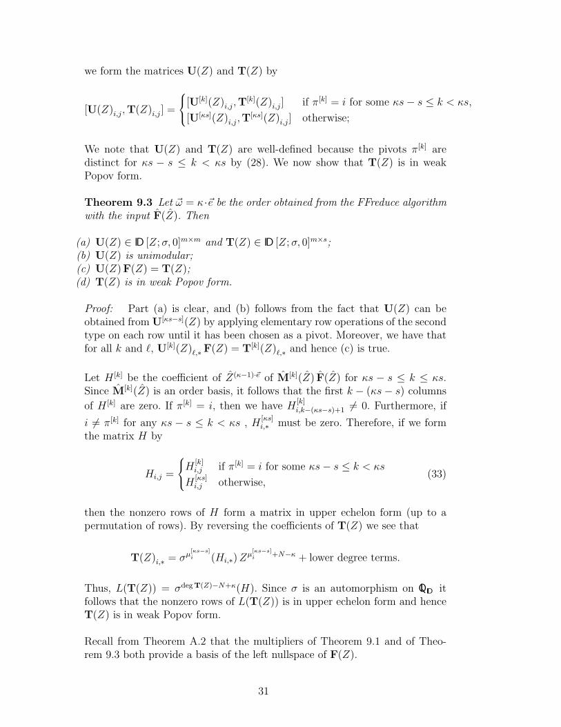
we form the matrices U(Z) and T(Z) by
[U(Z)i,j,T(Z)i,j] =
[U[k](Z)i,j,T[k](Z)i,j] if π[k] = i for some κs− s ≤ k < κs,
[U[κs](Z)i,j,T[κs](Z)i,j] otherwise;
We note that U(Z) and T(Z) are well-defined because the pivots π[k] aredistinct for κs − s ≤ k < κs by (28). We now show that T(Z) is in weakPopov form.
Theorem 9.3 Let ~ω = κ·~e be the order obtained from the FFreduce algorithmwith the input F(Z). Then
(a) U(Z) ∈ ID [Z;σ, 0]m×m and T(Z) ∈ ID [Z;σ, 0]m×s;(b) U(Z) is unimodular;(c) U(Z) F(Z) = T(Z);(d) T(Z) is in weak Popov form.
Proof: Part (a) is clear, and (b) follows from the fact that U(Z) can beobtained from U[κs−s](Z) by applying elementary row operations of the secondtype on each row until it has been chosen as a pivot. Moreover, we have thatfor all k and `, U[k](Z)`,∗F(Z) = T[k](Z)`,∗ and hence (c) is true.
Let H [k] be the coefficient of Z(κ−1)·~e of M[k](Z) F(Z) for κs − s ≤ k ≤ κs.Since M[k](Z) is an order basis, it follows that the first k − (κs− s) columns
of H [k] are zero. If π[k] = i, then we have H[k]i,k−(κs−s)+1 6= 0. Furthermore, if
i 6= π[k] for any κs − s ≤ k < κs , H[κs]i,∗ must be zero. Therefore, if we form
the matrix H by
Hi,j =
H[k]i,j if π[k] = i for some κs− s ≤ k < κs
H[κs]i,j otherwise,
(33)
then the nonzero rows of H form a matrix in upper echelon form (up to apermutation of rows). By reversing the coefficients of T(Z) we see that
T(Z)i,∗ = σµ[κs−s]i (Hi,∗)Z
µ[κs−s]i +N−κ + lower degree terms.
Thus, L(T(Z)) = σdeg T(Z)−N+κ(H). Since σ is an automorphism on QID itfollows that the nonzero rows of L(T(Z)) is in upper echelon form and henceT(Z) is in weak Popov form.
Recall from Theorem A.2 that the multipliers of Theorem 9.1 and of Theo-rem 9.3 both provide a basis of the left nullspace of F(Z).
31

9.3 Computing GCRD and LCLM of Matrices of Skew Polynomials
Using the preceding algorithm for row reduction allows us to compute a great-est common right divisor (GCRD) and a least common left multiple (LCLM)of matrices of skew polynomials in the same way it is done in the case ofmatrices of polynomials [Beckermann and Labahn, 2000, Kailath, 1980]. LetA(Z) ∈ ID [Z;σ, 0]m1×s and B(Z) ∈ ID [Z;σ, 0]m2×s, such that the matrix
F(Z) =
A(Z)
B(Z)
has rank s. Such an assumption is natural since otherwise we may have GCRDsof arbitrarily high degree [Kailath, 1980, page 376]. After row reduction andpossibly a permutation of the rows, we obtain
U(Z) F(Z) =
U11(Z) U12(Z)
U21(Z) U22(Z)
·A(Z)
B(Z)
=
G(Z)
0
(34)
with G(Z) ∈ ID [Z;σ, 0]s×s, and U1,j(Z), U2,j(Z) matrices of skew polynomialsof size s×mj, and (m1 +m2−s)×mj, respectively. Standard arguments (see,for example, Kailath [1980]) show that G(Z) is a GCRD of A(Z) and B(Z).Furthermore, for any common left multiple V1(Z) A(Z) = V2(Z) B(Z) we see
that the rows of[V1(Z) −V2(Z)
]belong to the left nullspace NF(Z). Since[
U21(Z) U22(Z)
]is a basis of NF(Z) by Theorem A.2, there exists Q(Z) ∈
QID [Z;σ, 0](m1+m2−s)×(m1+m2−s) such that[V1(Z) −V2(Z)
]= Q(Z)
[U21(Z) U22(Z)
],
implying that U21(Z) A(Z) and −U22(Z) B(Z) are LCLMs of A(Z) andB(Z).
In contrast to the method proposed in Beckermann and Labahn [2000], ourGCRD has the additional property of being row-reduced or being in weakPopov form.
9.4 Computation of Subresultants
The method of Section 9.3, applied to two 1×1 matrices, gives the GCRD andLCLM of two skew polynomials a(Z) and b(Z). In this subsection we examinethe relationship of the intermediate results obtained during our algorithm to
32
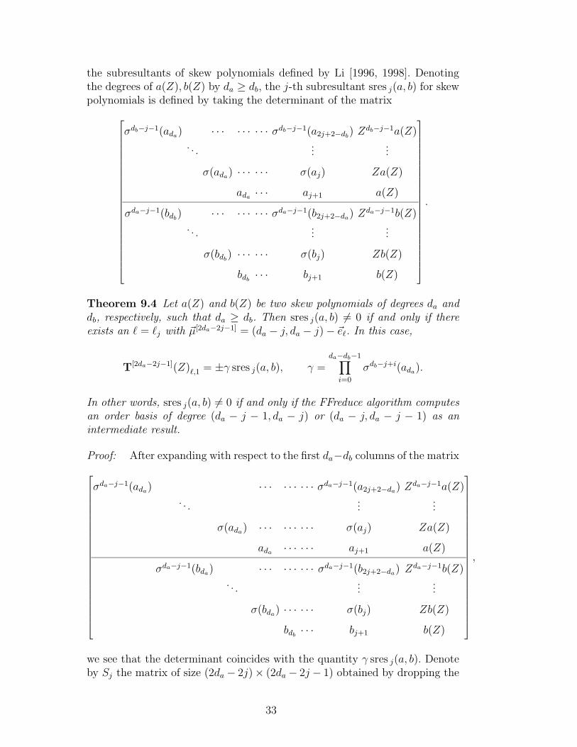
the subresultants of skew polynomials defined by Li [1996, 1998]. Denotingthe degrees of a(Z), b(Z) by da ≥ db, the j-th subresultant sres j(a, b) for skewpolynomials is defined by taking the determinant of the matrix
σdb−j−1(ada) · · · · · · · · · σdb−j−1(a2j+2−db) Zdb−j−1a(Z)
. . ....
...
σ(ada) · · · · · · σ(aj) Za(Z)
ada · · · aj+1 a(Z)
σda−j−1(bdb) · · · · · · · · · σda−j−1(b2j+2−da) Zda−j−1b(Z)
. . ....
...
σ(bdb) · · · · · · σ(bj) Zb(Z)
bdb · · · bj+1 b(Z)
.
Theorem 9.4 Let a(Z) and b(Z) be two skew polynomials of degrees da anddb, respectively, such that da ≥ db. Then sres j(a, b) 6= 0 if and only if thereexists an ` = `j with ~µ[2da−2j−1] = (da − j, da − j)− ~e`. In this case,
T[2da−2j−1](Z)`,1 = ±γ sres j(a, b), γ =da−db−1∏i=0
σdb−j+i(ada).
In other words, sres j(a, b) 6= 0 if and only if the FFreduce algorithm computesan order basis of degree (da − j − 1, da − j) or (da − j, da − j − 1) as anintermediate result.
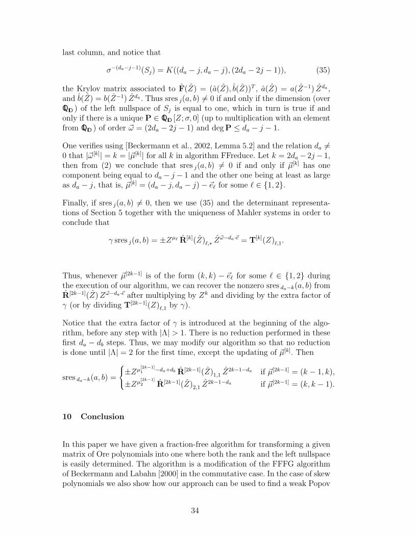
Proof: After expanding with respect to the first da−db columns of the matrix
σda−j−1(ada) · · · · · · · · · σda−j−1(a2j+2−da) Zda−j−1a(Z)
. . ....
...
σ(ada) · · · · · · · · · σ(aj) Za(Z)
ada · · · · · · aj+1 a(Z)
σda−j−1(bda) · · · · · · · · · σda−j−1(b2j+2−da) Zda−j−1b(Z)
. . ....
...
σ(bda) · · · · · · σ(bj) Zb(Z)
bdb · · · bj+1 b(Z)
,
we see that the determinant coincides with the quantity γ sres j(a, b). Denoteby Sj the matrix of size (2da − 2j)× (2da − 2j − 1) obtained by dropping the
33
last column, and notice that
σ−(da−j−1)(Sj) = K((da − j, da − j), (2da − 2j − 1)), (35)
the Krylov matrix associated to F(Z) = (a(Z), b(Z))T , a(Z) = a(Z−1) Zda ,and b(Z) = b(Z−1) Zda . Thus sres j(a, b) 6= 0 if and only if the dimension (overQID ) of the left nullspace of Sj is equal to one, which in turn is true if andonly if there is a unique P ∈ QID [Z;σ, 0] (up to multiplication with an elementfrom QID ) of order ~ω = (2da − 2j − 1) and deg P ≤ da − j − 1.
One verifies using [Beckermann et al., 2002, Lemma 5.2] and the relation da 6=0 that |~ω[k]| = k = |~µ[k]| for all k in algorithm FFreduce. Let k = 2da− 2j− 1,then from (2) we conclude that sres j(a, b) 6= 0 if and only if ~µ[k] has onecomponent being equal to da− j − 1 and the other one being at least as largeas da − j, that is, ~µ[k] = (da − j, da − j)− ~e` for some ` ∈ {1, 2}.
Finally, if sres j(a, b) 6= 0, then we use (35) and the determinant representa-tions of Section 5 together with the uniqueness of Mahler systems in order toconclude that
γ sres j(a, b) = ±Zµ` R[k](Z)`,∗ Z~ω−da·~e = T[k](Z)`,1.
Thus, whenever ~µ[2k−1] is of the form (k, k) − ~e` for some ` ∈ {1, 2} duringthe execution of our algorithm, we can recover the nonzero sres da−k(a, b) fromR[2k−1](Z)Z~ω−da·~e after multiplying by Zk and dividing by the extra factor ofγ (or by dividing T[2k−1](Z)`,1 by γ).
Notice that the extra factor of γ is introduced at the beginning of the algo-rithm, before any step with |Λ| > 1. There is no reduction performed in thesefirst da − db steps. Thus, we may modify our algorithm so that no reductionis done until |Λ| = 2 for the first time, except the updating of ~µ[k]. Then
sres da−k(a, b) =
±Zµ[2k−1]1 −da+db R[2k−1](Z)1,1 Z
2k−1−da if ~µ[2k−1] = (k − 1, k),
±Zµ[2k−1]2 R[2k−1](Z)2,1 Z
2k−1−da if ~µ[2k−1] = (k, k − 1).
10 Conclusion
In this paper we have given a fraction-free algorithm for transforming a givenmatrix of Ore polynomials into one where both the rank and the left nullspaceis easily determined. The algorithm is a modification of the FFFG algorithmof Beckermann and Labahn [2000] in the commutative case. In the case of skewpolynomials we also show how our approach can be used to find a weak Popov
34
form of a matrix of skew polynomials. In addition, in the special case of 2× 1skew polynomial matrices we relate our algorithm along with the intermediatequantities to the classical subresultants typically used for one sided GCD andLCM computations.
There are a number of topics for future research. In this paper we have givena fraction-free method for elimination of low order terms of a matrix of Orepolynomials. However for general Ore domains it appears to be more usefulto work with leading coefficients, something not possible using our methodsexcept for the case of skew-polynomial domains. We note that this is possibleto do using the approach of Abramov and Bronstein simply by using Theorem2.2. In our case we would like to find a fraction-free method for such a reductionover Ore domains. We will look at combining the procedure in Theorem 2.2along with modified Schur complements [Beckermann et al., 1997] of Krylovmatrices to help us develop such an algorithm.
In a recent work Abramov and Bronstein [2002] extend their results to handlethe case of nested skew Ore domains, allowing for computations for example inWeyl algebras. We would like to extend our methods to this important class ofmatrices again with the idea of controlling the growth of the resulting matrices.This is a difficult extension to do using the methods described in our papersince the corresponding associated linear systems do not have commutativeelements. As such the standard tools that we use from linear algebra, namelydeterminants and Cramer’s rule, do not exist in the classical sense.
Finally, it is well known that modular algorithms improve on fraction-freemethods by an order of magnitude. We plan to investigate such algorithmsfor our rank and left nullspace computations. We note that the determinantalrepresentations gives a first step in this direction since it provides an upperbound for the sizes of the objects which need to be computed. As in themodular algorithm for computing a GCRD of Ore polynomials [Li, 1996, Liand Nemes, 1997], we expect that the fraction-free algorithm would be a basisfor the modular algorithm.
References
S. Abramov. EG-eliminations. Journal of Difference Equations and Applica-tions, 5(393–433), 1999.
S. Abramov and M. Bronstein. On solutions of linear functional systems. InProceedings of the 2001 International Symposium on Symbolic and AlgebraicComputation, pages 1–6. ACM, 2001.
S. Abramov and M. Bronstein. Linear algebra for skew-polynomial matrices.Technical Report RR-4420, Rapport de Recherche INRIA, 2002.
35
E. Bareiss. Sylvester’s identity and multistep integer-preserving Gaussianelimination. Mathematics of Computation, 22(103):565–578, 1968.
B. Beckermann, S. Cabay, and G. Labahn. Fraction-free computation of ma-trix Pade systems. In Proceedings of the 1997 International Symposium onSymbolic and Algebraic Computation, pages 125–132. ACM, 1997.
B. Beckermann, H. Cheng, and G. Labahn. Fraction-free row reduction of ma-trices of skew polynomials. In Proceedings of the 2002 International Sym-posium on Symbolic and Algebraic Computation, pages 8–15. ACM, 2002.
B. Beckermann and G. Labahn. Recursiveness in matrix rational interpolationproblems. Journal of Computational and Applied Mathematics, 77:5–34,1997.
B. Beckermann and G. Labahn. Fraction-free computation of matrix GCD’sand rational interpolants. SIAM Journal on Matrix Analysis and Applica-tions, 22(1):114–144, 2000.
B. Beckermann, G. Labahn, and G. Villard. Normal forms for general poly-nomial matrices. To appear in Journal of Symbolic Computation, 2001.
P. M. Cohn. Free Rings and Their Relations. Academic Press, 1971.T. Kailath. Linear Systems. Prentice-Hall, 1980.Z. Li. A Subresultant Theory for Linear Differential, Linear Difference and
Ore Polynomials, with Applications. PhD thesis, Johannes Kepler UniversityLinz, Austria, 1996.
Z. Li. A subresultant theory for Ore polynomials with applications. In Pro-ceedings of the 1998 International Symposium on Symbolic and AlgebraicComputation, pages 132–139. ACM, 1998.
Z. Li. Private communication, 2003.Z. Li and I. Nemes. A modular algorithm for computing greatest common
right divisors of Ore polynomials. In Proceedings of the 1997 InternationalSymposium on Symbolic and Algebraic Computation, pages 282–289. ACM,1997.
T. Mulders and A. Storjohann. On lattice reduction for polynomial matrices.Journal of Symbolic Computation, 35(4):377–401, 2003.
A Appendix: Further Facts on Matrices of Ore Polynomials
In this appendix we will present a number of technical results that are neededin our paper. These results are typically well understood in the context ofcommutative matrix polynomials but are not at all obvious for the case ofnoncommutative matrices of Ore polynomials.
Consider first the notion of the rank of a matrix of Ore polynomials, F(Z) ∈IK [Z;σ, δ]m×s. Denote by MF(Z) = {Q(Z)F(Z) : Q(Z) ∈ IK [Z;σ, δ]1×m}the submodule of the (left) IK [Z;σ, δ]-module ⊂ IK [Z;σ, δ]1×s obtained byforming left linear combinations of the rows of F(Z). Then following [Cohn,
36
1971, p. 28, Section 0.6], the rank of a module M over IK [Z;σ, δ] is definedto be the cardinality of a maximal IK [Z;σ, δ]-linearly independent subset ofM. Comparing with our Definition 2.1, we see that rank F(Z) ≤ rankMF(Z).Theorem A.2 below shows that in fact we have equality.
Notice that for any A(Z) ∈ IK [Z;σ, δ]m×m we have thatMA(Z)F(Z) ⊂MF(Z).If now A(Z) has a left inverse V(Z) ∈ IK [Z;σ, δ]m×m, then we also have theinclusions MF(Z) = MV(Z)A(Z)F(Z) ⊂ MA(Z)F(Z), showing that in this caseMA(Z)F(Z) =MF(Z).
For identifying the different concepts of rank, it will be useful to show that therows of a row-reduced matrix of Ore polynomials are linearly independent overIK [Z;σ, δ]. This however is an immediate consequence of Lemma A.1(a) belowwhich in case of ordinary matrix polynomials is referred to as the predictabledegree property (see Kailath [1980], Theorem 6.3.13).
Lemma A.1 Let F(Z) ∈ IK [Z;σ, δ]m×s, with ~µ = row-deg F(Z).
(a) F(Z) is row-reduced if and only if, for all Q(Z) ∈ IK [Z;σ, δ]1×m,
deg Q(Z)F(Z) = maxj
(µj + deg Q(Z)1,j).
(b) Let A(Z) = B(Z) C(Z) be matrices of Ore polynomials of sizes m × s,m× r, and r × s, respectively. Then rank A(Z) ≤ r.
(c) Let A(Z) = B(Z) C(Z) be as in part (b), with A(Z) and C(Z) row-reduced with row degrees α1 ≤ α2 ≤ ... ≤ αm and γ1 ≤ γ2 ≤ ... ≤ γr,respectively. Then m ≤ r, and αj ≥ γj for j = 1, ...,m.
(d) Let T(Z) = U(Z) S(Z), with U(Z) unimodular and with both S(Z) andT(Z) row-reduced. Then, up to permutation, the row degrees of S(Z) andT(Z) coincide.
Proof: For any Q(Z) ∈ IK [Z;σ, δ]1×m let N ′ := maxj(µj + deg Q(Z)1,j
)and define the vector ~h ∈ IK 1×m, ~h 6= ~0, by
Q(Z)1,j = hjZN ′−µj + lower degree terms.
Clearly, deg Q(Z) F(Z) ≤ N ′, with the coefficient at ZN ′ being given by
m∑j=1
hjσN ′−µj(F
(µj)j,∗ ) = ~h σN
′−N(L(F(Z))).
Since σ is injective, we have that F(Z) is row-reduced if and only if σj(L(F(Z)))is of full row rank for any integer j that is, if and only if hσj(L(F(Z))) 6=0 for all h 6= 0 and all integers j. This in turn holds true if and only ifdeg Q(Z)F(Z) = N ′ for any Q(Z) ∈ IK [Z;σ, δ]1×m.
37
In order to show (b), we may suppose by eliminating a suitable number ofrows of A(Z) and B(Z) that rank A(Z) = m. If r < m, then MB(Z) ⊂IK [Z;σ, δ]1×r, the latter IK [Z;σ, δ]-module being of rank r. Hence r ≥ rankMB(Z) ≥rank B(Z). On the other hand, B(Z) has more rows than columns. Thus, bydefinition of rank B(Z) there exists a nontrivial Q(Z) ∈ IK [Z;σ, δ]1×m withQ(Z)B(Z) = 0. Thus Q(Z)A(Z) = 0, a contradiction to the fact that A(Z)has full row rank m. Therefore r ≥ m, as claimed in part (b).
For a proof of part (c), recall first that the rows of the row-reduced A(Z) areIK [Z;σ, δ]-linearly independent by part (a), and hence m = rank A(Z) ≤ r bypart (b). Suppose that αj ≥ γj for j < k, but αk < γk. Part (a) tells us thatdeg B(Z)j,` ≤ αj − γ`. Since αj < γk ≤ γ` for j ≤ k ≤ `, we may concludethat B(Z)j,` = 0 for j ≤ k ≤ `, in other words, the first k rows of A(Z) areleft polynomial combinations of the first k− 1 rows of C(Z). Again from part(b) it follows that the first k rows of A(Z) are IK [Z;σ, δ]-linearly dependent,a contradiction. Hence the assertion of part (c) holds.
Finally, part (d) is obtained by twice applying part (c) (compare with [Kailath,1980, Lemma 6.3.14, p.388] for the case of ordinary matrix polynomials).
Consider now the left nullspace NF(Z) of a F(Z) ∈ IK [Z;σ, δ]m×s. Clearly,NF(Z) is a IK [Z;σ, δ]-module. We want to construct a row-reduced basis ofthis space, and obtain information about the degrees of such a basis.
Theorem A.2 Let F(Z) ∈ IK [Z;σ, δ]m×s, and U(Z) ∈ IK [Z;σ, δ]m×m be uni-modular, with T(Z) = U(Z) F(Z) having r nonzero rows, where the submatrixconsisting of the r nonzero rows of T(Z) are row-reduced. Then
r = rankMF(Z) = rank F(Z) = m− rankNF(Z), (A.1)
with a basis over IK [Z;σ, δ] of NF(Z) given by those rows of U(Z) correspondingto the zero rows of T(Z).
Moreover, there exists a row-reduced W(Z) ∈ IK [Z;σ, δ](m−r)×m with rowsforming a basis of the left nullspace NF(Z), and
row-deg W(Z) ≤ (m− 1)N~e, N = deg F(Z).
Proof: Denote by J the set of indices of zero rows of T(Z), and define thematrix U(Z)J,∗ by extracting from U(Z) the rows with indices in J . In a firststep, let us determine the left nullspace of T(Z), and establish equality (A.1)for the matrix T(Z). For some P(Z) ∈ IK [Z;σ, δ]1×m we have
P(Z)T(Z) =∑j 6∈J
P(Z)1,jT(Z)j,∗.
38
We have shown implicitly in Lemma A.1(a) that the rows T(Z)j,∗ for j 6∈ Jare linearly independent over IK [Z;σ, δ]. Therefore P(Z) ∈ NT(Z) if and onlyif P(Z)1,j = 0 for all j 6∈ J , and in addition
r = rank T(Z) = m− rankNT(Z).
As mentioned before, we also have that rank T(Z) ≤ rankMT(Z) =: ρ. Sup-pose that there is strict inequality. Then there exist ρ elements ofMT(Z) whichare IK [Z;σ, δ]-linearly independent and which can be written as rows of thematrix B(Z)T(Z) for some B(Z) ∈ IK [Z;σ, δ]ρ×m. Then rank B(Z)T(Z) = ρby construction of B(Z). However T(Z) contains only r rows different fromzero, and hence rank B(Z)T(Z) ≤ r by Lemma A.1(b), a contradiction. Con-sequently, (A.1) holds for the matrix F(Z) being replaced by T(Z).
We now use the fact that U(Z) is unimodular, that is, there exists a V(Z) ∈IK [Z;σ, δ]m×m with V(Z) U(Z) = U(Z) V(Z) = I. Consequently, Q(Z) ∈NF(Z) if and only if P(Z) = Q(Z) V(Z) ∈ NT(Z), that is,
NF(Z) = {P(Z) U(Z) : P(Z)1,j = 0 for j 6∈ J} =MU(Z)J,∗.
Since U(Z) has a right inverse, we may conclude that NU(Z) = {0}, showingthat rows of unimodular matrices are linearly independent over IK [Z;σ, δ].Thus the rows of U(Z)J,∗ form a basis of NF(Z), and
m− rankMF(Z) = m− rankMT(Z) = m− r = rankNF(Z).
Since again the relation ρ := rank F(Z) ≤ rankMF(Z) is trivial, for a proofof the first part of the assertion of Theorem A.2 it only remains to show thatρ < r leads to a contradiction. Suppose without loss of generality that thefirst ρ rows of F(Z) are linearly independent. Then, by maximality of ρ, wefind for any j = ρ+ 1, ...,m quantities Q(Z)j,k ∈ IK [Z;σ, δ] with
Q(Z)j,j 6= 0, Q(Z)j,jF(Z)j,∗ +ρ∑
k=1
Q(Z)j,kF(Z)k,∗ = 0,
that is, we have found m − ρ > m − r many IK [Z;σ, δ]-linearly independentelements of NF(Z), in contradiction to our previous findings on rankNF(Z).
In order to show the second part of Theorem A.2, suppose that U(Z) and T(Z)are those defined in Theorem 2.2. Let W(Z) be the row-reduced counterpartof U(Z)J,∗ obtained by applying Theorem 2.2. Since one is obtained from theother by multiplying on the left by some unimodular factor, the rows of W(Z)form a row-reduced basis of NF(Z), with row-deg W(Z) ≤ row-deg U(Z)J,∗.Hence it only remains to recall the bound for the row-degree of the multiplierU(Z) of Theorem 2.2: we have for j ∈ J
deg U(Z)j,∗ ≤ νj − µj + (|~µ| − |~ν|) ≤ |~µ| − ~µj ≤ (m− 1)N.
39
We should mention that the quantity row-deg W(Z) of Theorem A.2 is aninvariant of F(Z) since by Lemma A.1(d), we obtain the same degrees (upto permutation) for any row-reduced basis of the left nullspace of F(Z). Inthe case of ordinary matrix polynomials, the components of row-deg W(Z)are usually referred to as left minimal indices or left Kronecker indices, (see§6.5.4, p. 456 of Kailath [1980]).
We conclude this appendix by showing that a certain number of elementaryproperties of the rank remain equally valid for matrices of Ore polynomials.
Lemma A.3 For any F(Z) ∈ IK [Z;σ, δ]m×s, the rank of F(Z) does not changeby applying any of the row operations of first or second type described in theintroduction, or by multiplying F(Z) on the right by a full rank square matrixof Ore polynomials.
Proof: Suppose that A(Z) ∈ IK [Z;σ, δ]s×s is of rank s. Then NA(Z) = {0}by (A.1), implying that NF(Z)A(Z) = NF(Z). Hence F(Z)A(Z) and F(Z) havethe same rank by (A.1). If U(Z) is unimodular, then MU(Z) F(Z) = MF(Z),showing that the rank remains the same. Finally we need to examine the rowoperation of multiplying one row of F(Z) with a nonzero element of IK [Z;σ, δ].Since IK [Z;σ, δ] contains no zero divisors, it is easy to check that F(Z) andthe new matrix will have the same number of IK [Z;σ, δ]-linearly independentrows, and hence the same rank.
40