Fractal properties of forest fires in Amazonia as a basis for.pdf

Biogeosciences, 11, 1449–1459, 2014www.biogeosciences.net/11/1449/2014/doi:10.5194/bg-11-1449-2014© Author(s) 2014. CC Attribution 3.0 License.

Biogeosciences

Open A

ccess

Fractal properties of forest fires in Amazonia as a basis formodelling pan-tropical burnt area

I. N. Fletcher1, L. E. O. C. Aragão2,3, A. Lima3, Y. Shimabukuro3, and P. Friedlingstein1

1College of Engineering, Mathematics and Physical Sciences, University of Exeter, Exeter EX4 4QF, UK2College of Life and Environmental Sciences, University of Exeter, Exeter EX4 4RJ, UK3National Institute for Space Research, Remote Sensing Division, São José dos Campos SP-12227-010, Brazil

Correspondence to:I. N. Fletcher ([email protected])

Received: 16 July 2013 – Published in Biogeosciences Discuss.: 26 August 2013Revised: 7 February 2014 – Accepted: 12 February 2014 – Published: 19 March 2014

Abstract. Current methods for modelling burnt area in dy-namic global vegetation models (DGVMs) involve complexfire spread calculations, which rely on many inputs, includ-ing fuel characteristics, wind speed and countless param-eters. They are therefore susceptible to large uncertaintiesthrough error propagation, but undeniably useful for mod-elling specific, small-scale burns. Using observed fractal dis-tributions of fire scars in Brazilian Amazonia in 2005, wepropose an alternative burnt area model for tropical forests,with fire counts as sole input and few parameters. This modelis intended for predicting large-scale burnt area rather thanlooking at individual fire events. A simple parameterizationof a tapered fractal distribution is calibrated at multiple spa-tial resolutions using a satellite-derived burnt area map. Themodel is capable of accurately reproducing the total areaburnt (16 387 km2) and its spatial distribution. When testedpan-tropically using the MODIS MCD14ML active fire prod-uct, the model accurately predicts temporal and spatial firetrends, but the magnitude of the differences between theseestimates and the GFED3.1 burnt area products varies percontinent.

1 Introduction

Fires are a major component of the global carbon cycle.Globally, they release an average of 2.0 PgCyr−1 into the at-mosphere and over a third of this amount can be attributed totropical fires (van der Werf et al., 2010). A changing climateis expected to increase the occurrence of droughts in tropi-cal regions (e.g.Booth et al., 2012; Cox et al., 2008), which

in turn will make extreme tropical fire regimes more likely(Aragão et al., 2007; van der Werf et al., 2008).

Despite their importance, representing fire dynamicswithin dynamic global vegetation models (DGVMs) tomodel their impacts upon the structure and functioning ofecosystems and their potential feedbacks on the climate sys-tem has been challenging. Their accuracy depends, in part,on an accurate representation of fire dynamics, yet manyDGVMs do not contain a wildfire component (Piao et al.,2013). For quantifying carbon emissions from fires, threemain steps are required: (i) predicting how many fires willoccur, (ii) modelling the spread of these fires in order to de-termine burnt area, and (iii) calculating the expected quantityof biomass that will be combusted as a result. In this studywe focus specifically on the second of these steps.

Within existing fire models, the spread of fire is one ofthe more complex processes. Many fire models implementedin DGVMs – including the most detailed fire models todate, SPITFIRE (Thonicke et al., 2010) and its successor, thefire component of LPX (Prentice et al., 2011) – use an ap-proach based on the Rothermel equations (Rothermel, 1972)to model the rate of fire spread. The area burnt in a givengrid cell is then calculated using the rate of spread, expectednumber of ignitions and calculated fire danger index. Thisestimate relies on the assumption that fires generate ellipticalburn scars. The Rothermel approach requires data about thedistribution, density and moisture content of fuel in the area,the velocity of wind, and assumptions about when fires stopspreading. Data about the fuel needed to sustain fire spreadare generally calculated by the DGVM itself, and thereforeprone to substantial uncertainties. Wind velocity is routinely

Published by Copernicus Publications on behalf of the European Geosciences Union.

1450 I. N. Fletcher et al.: Modelling tropical forest burnt area

measured at meteorological stations; however, the accuracyof wind estimates from climate models that extend past thetime frame of available measurements is uncertain, furtherlimiting the potential of such an approach for palaeontolog-ical or future projections of fires. Additionally, a large num-ber of prescribed parameters are used to describe processessuch as the effect of damp fuel combustion on fire inten-sity. These parameters are generally estimated, and thereforelikely to differ from their true values. Hence, each additionalparameter introduces a new level of uncertainty into the mod-elled fire simulations. Because simulated area burnt is depen-dent on several separate assumptions, expressed as paramet-ric equations, its accuracy is highly susceptible to both pa-rameterization and forcing data errors, especially for tropicalforest ecosystems.

It is undeniable that fire spread, as a physical process, mustbe dependent on ecological and climatic conditions, and thatdetails of these conditions are essential for predicting thespread of any individual fire. The traditional approach ofmodelling the spread of individual fire events requires de-tailed, localized data such as wind speed, fuel moisture andfuel loading. However, if the aim is to estimate the total burntarea resulting from all fires in a given region or biome over acertain time period, we can greatly reduce the number of in-put data sets required. For the model developed in this study,by using the theory of a scale-invariant fire size distribution,we need only ecological information about the dominant landcover type of the study area.

Scale invariance manifests itself as a fractal distribution,where the probability that an event of a certain size will oc-cur decreases proportionally as the size increases. The exactdistribution that is appropriate for a given system is debat-able, and a range of possibilities are suggested in the liter-ature. It has been shown that a huge range of complex dy-namical systems and extreme events are scale-invariant, fromearthquakes (Sornette and Sornette, 1989) and solar flares(Bofetta et al., 1999), to the extinction of species (Solé andManrubia, 1996). More importantly for this work, numer-ous studies have shown scale invariance in the distribution ofwildfire sizes, for certain regions and time frames (Cui andPerera, 2008). Significant power-law distributions of fireswere found in regions of the US and Australia (Malamudet al., 1998), Spain (Moreno et al., 2011) and Amazonia(Pueyo et al., 2010). Some studies showed that either a trun-cated, piecewise or tapered distribution might be more ap-propriate for certain regions (Cumming, 2001; Holmes et al.,2004; Ricotta et al., 1999; Schoenberg et al., 2003; Pueyoet al., 2010) than an unbounded one.

The consensus among these studies is that variation in theparameters of these distributions between ecosystems and re-gions is associated with differences in land cover and localclimate, and as such there has been no previous attempt togeneralize the distributions over larger regions and time peri-ods. In this study, we consider only tropical forests. Althoughthere is variability in land cover within tropical forests, we do

not investigate the effect of land cover on the distribution pa-rameters in this study. Local climate affects both the numberof fires or fire fronts that occur as well as the spread of thesefires. However, in this study we hypothesize that the effectsof climate variations on active fires and fire spread are closelycorrelated, and hence, if fire counts are known, then the dis-tribution parameters can be estimated from this single inputvariable, without the introduction of a weather variable.

To test this hypothesis, we proceed in three successivesteps. First, we identify a distribution that is a suitable ap-proximation of the observed distribution of fire sizes in theforests of Brazilian Amazonia. Second, we develop methodsfor estimating the distribution parameters, and check the ac-curacy of the model simulations of both the spatial distri-bution and total accumulation of burnt area across the wholeregion. Third, we test the suitability of the model for use withall tropical forests, as well as its ability to capture both spatialand temporal patterns of burnt area.

2 Model development

2.1 Data

In this work we used a burn scar data set for 2005 pro-duced byLima et al.(2009), restricted to the forested areaswithin the Brazilian Legal Amazonia limits, to calibrate themodel. The burn scars were mapped using a linear spectralmixing model (LSMM;Shimabukuro and Smith, 1991) ap-plied to the MOD09 daily reflectance product from ModerateResolution Imaging Spectroradiometer (MODIS) onboard ofNASA’s Terra satellite, using the red (band 1), near-infrared(band 2) and short-wave infrared (band 6) bands at a 250 mspatial resolution (Justice et al., 2002) (band 6 data wereregridded from its original 500 m resolution). The MODISimages were chosen based on the following criteria: (1) im-ages should be within the fire season period, identified byanalysing daily active fire information from MYD14 prod-uct; (2) images should be free or partially free cloud images;and (3) images should be acquired with a view angle close tothe nadir to minimize panoramic distortion.

The mapping was carried out in four steps, following themethods ofShimabukuro et al.(2009): application of anLSMM, segmentation of shade fraction image, unsupervisedclassification by regions and visual interpretation.

The LSMM was applied to the composite bands 1, 2 and 6to generate the shade fraction image, which highlights low-reflectance targets – the case of burnt areas. Shade fractionimages were subsequently classified in two steps. The firstconsisted in the application of a segmentation algorithm. Thesecond encompassed the use of an unsupervised classifica-tion method (ISOSEG,Ball and Hall, 1965; Kawakubo et al.,2013) applied to the segmented images.

For the segmentation procedure two thresholds were de-fined: (a) the similarity threshold, a minimum threshold

Biogeosciences, 11, 1449–1459, 2014 www.biogeosciences.net/11/1449/2014/

I. N. Fletcher et al.: Modelling tropical forest burnt area 1451

below which two regions are considered similar and groupedinto a single polygon, and (b) the threshold area, minimumarea value, given in pixels numbers, for a region to be in-dividualized. A value of eight digital numbers and an areaequal to four pixels were used for the similarity and areathreshold, respectively. These thresholds were set based onthe complexity of shape and size as well as from the meandeviations of digital number values of burn scars samples vi-sually identified.

After segmentation, the ISOSEG algorithm was appliedto the three bands generated by the LSMM, shade, soil andvegetation with a 75 % similarity limit (Shimabukuro et al.,2009). From the resulting classes, those corresponding toburnt areas were merged into a single “burn scar” class, andthe remaining classes were discarded.

All water bodies were masked out and editing based onvisual interpretation was performed to differentiate betweenburn scars and terrain shadow. All maps produced for eachdate were combined into a single yearly map depicting thetotal area of burn scars in 2005.

Finally, to quantify the forest burnt area, the burn scarsmap generated was overlapped by the 2005 forest mask pro-vided by PRODES project (INPE, 2013). The final map usedfor the model calibration was the result of the intersectionbetween the burn scars and PRODES forest area maps.

We compare the total area of burn scars mapped with ahigher resolution map (30 m spatial resolution) derived fromvisual classification of Landsat 5/TM false-colour compositescenes for three Amazonian states following a west-to-easttransect: (1) Acre (path 001/row 67), (2) Amazonas (path230/row 65) and (3) Maranhao (path 221/ row 65). For theclassification of the total burnt area for 2005 based on Land-sat 5/TM data we used seven, five and six cloud-free scenesacquired during the fire season for Acre, Amazonas andMaranhao, respectively. We also compare our results withthe MODIS burn scar product MCD45. Overall, using theLSMM algorithm produces a total area of burn scars consis-tent with the higher resolution map, apart from the state ofAmazonas, where an underestimation is clear. Surprisingly,the MCD45 product well underestimates the burn scar areafor the regions analysed in comparison to both Landsat 5/TMand our MODIS LSMM mapping procedure (Fig. S1, Sup-plement).

For the purpose of our analysis we used point data cor-responding to the LSMM image data, at a 500 m resolution.We treated every group of adjacent 500 m× 500 m pixels asa single fire event, and counted the number of fires of eachsize,A, in every grid cell, repeating the procedure for fourdifferent grid-cell resolutions: 0.5◦ × 0.5◦, 1◦

× 1◦, 2◦× 2◦

and 4◦ × 4◦. Any fire event that crossed a boundary betweentwo or more grid cells was attributed to the grid cell in whichthe majority of the burn scar could be found. In this way, weobtained information about the number of fires of each sizein each grid cell. Due to the use of logarithms in the distribu-tions, all calculations use the number of pixels as the fire size

measure, rather than an area value, to ensure that 0≤ log(A)

at all times.All analyses presented below were performed for each of

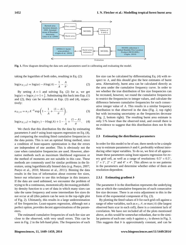
these four grid-cell resolutions in order to assess the effect ofchanging the resolution on the accuracy of the results. Thesuitability of the distribution for estimating burnt area wasassessed at both a grid-cell level and over the whole BrazilianAmazon domain. The exact use of this data set in the overallwork presented here is shown in Fig. 1.

2.2 Representing the fractal properties of fire sizedistributions

A range of distributions have been used in the literature to de-scribe fire size distributions. The most common is the Paretodistribution, sometimes referred to as the power-law distribu-tion. This states that the probability that fireX is of sizeA

or larger is proportional toA−b, for a constantb. Other stud-ies use variations of this distribution to allow for the fact thatfires in many regions show scale invariance only for a par-ticular range of sizes. One of these variations is truncation,i.e. ignoring all fires smaller than a lower threshold and/orlarger than some upper threshold. Although this yields inter-esting information about the behaviour of fires, it is not use-ful in the context of this study, since all fires must be consid-ered if an accurate prediction of burnt area is to be produced.Small fires contribute greatly to total burnt area:Randersonet al. (2012) found that accounting for small fires resultedin a 35 % increase in total global burnt area estimates. An-other variation prevalent in the literature is a piecewise dis-tribution, where the parameters of the Pareto distribution aredistinct for two or more ranges of fire sizes. Although possi-ble, this would require the estimation of many more param-eters, and hence could have a large effect on the accuracyof the model. The other commonly used option is to mod-ify the Pareto distribution to include a tapering function (e.g.Schoenberg et al., 2003). However, this generally only allowsfor the distribution to tail off as the fires become extremelylarge: it does not take into account the fact that there may bea tail at the low end of the distribution as well.

Based on the burn scar data we are using to calibrate themodel, we use the following distribution:

nX≥A = αA−b exp

(−

1

A−

A

θ

), (1)

wherenX≥A is the number of fires of sizeA or larger, andα, b andθ are grid-cell-dependent parameters.θ is known asthe tapering parameter. The−1/A term represents the small-fire taper. Although an additional parameter could be intro-duced into this term, this tapering is most likely a result oflimitations in the detection of small fires, and hence shouldremain constant. The estimate of such a parameter for thewhole region is 0.99±0.075 (using least-squares regression,as described below), so the use of the number 1 in this termis reasonable. For ease of use, Eq. (1) can be rewritten by

www.biogeosciences.net/11/1449/2014/ Biogeosciences, 11, 1449–1459, 2014


Fig. 1.Flow diagram detailing the data sets and parameters used in calibrating and evaluating the model.

taking the logarithm of both sides, resulting in Eq. (2):

log(nX≥A) = log(α) − b log(A) −1

A−

A

θ. (2)

By setting A = 1 and solving Eq. (2) for α, we getlog(α) = log(nf )+1+

1θ. Substituting this back into Eqs. (1)

and (2), they can be rewritten as Eqs. (3) and (4), respec-tively:

nX≥A = nf A−b exp

(1−

1

A+

(1− A)

θ

), (3)

log(nX≥A) = log(nf ) − b log(A) + 1−1

A+

(1− A)

θ. (4)

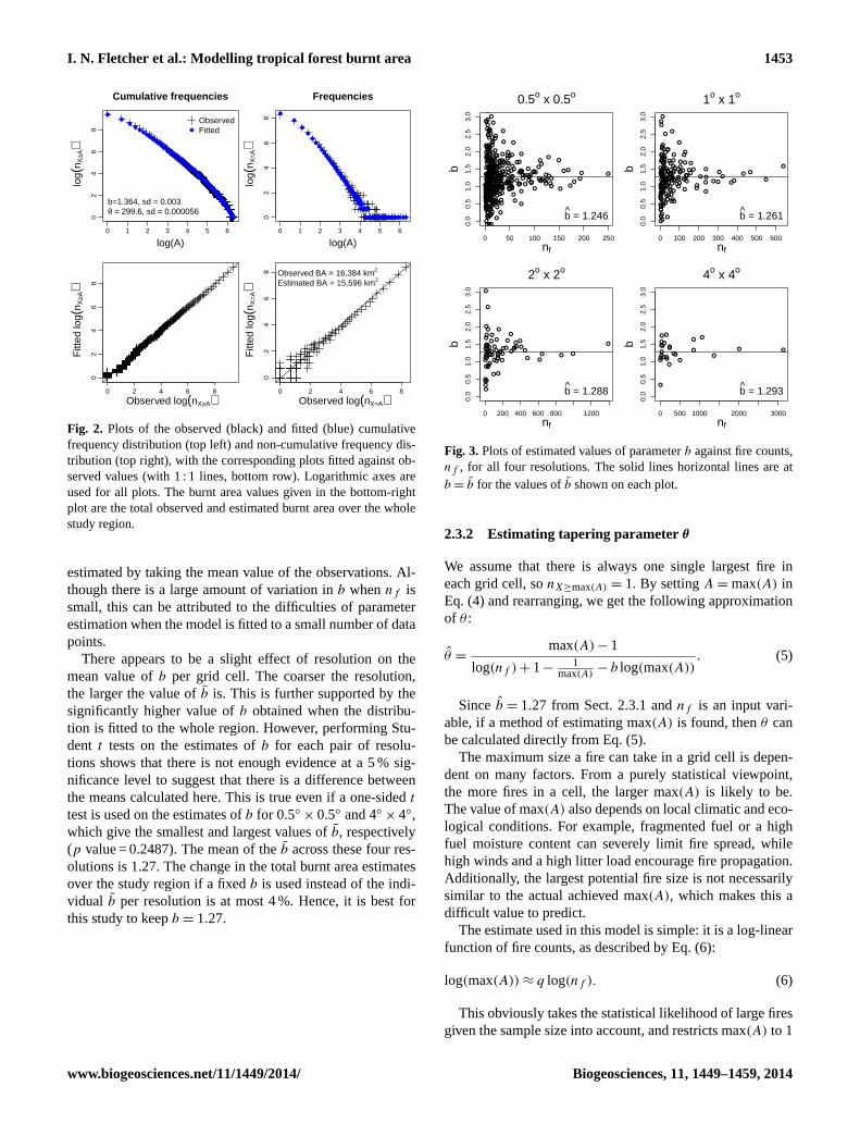
We check that this distribution fits the data by estimatingparametersb andθ using least-squares regression on Eq. (4),and comparing the resulting fitted cumulative frequencies tothe data points. This is not an optimal fitting method, sincea condition of least-squares optimization is that the errorsare independent of one another. This is obviously not thecase when cumulative frequencies are used. However, alter-native methods such as maximum likelihood regression orthe method of moments are not suitable in this case. Thesemethods are commonly used for similar problems in the lit-erature, using logarithmically binned data (e.g.Pueyo, 2007;Pueyo et al., 2010; Moreno et al., 2011). Binning the dataresults in the loss of information about extreme fire sizes,hence our reluctance to use this technique in this instance.If the data are used unbinned, we encounter the problem oftrying to fit a continuous, monotonically decreasing probabil-ity density function to a set of data in which many sizes cantake the same frequency and some intermediate fire sizes donot occur at all (this pattern can be seen in the top-right plotof Fig. 2). Ultimately, this results in a large underestimationof fire frequencies. Least-squares regression, although not aperfect option, provides decent approximations of the param-eters.

The estimated cumulative frequencies of each fire size areclose to the observed, with very small errors. This can beseen in Fig. 2 in the left-hand plots. The frequencies of each

fire size can be calculated by differentiating Eq. (4) with re-spect toA, and this should give the best estimates of burntarea. Alternatively, burnt area can be calculated directly asthe area under the cumulative frequency curve. In order tosee whether the true distribution of fire size frequencies canbe recreated, however, we round the cumulative frequenciesto restrict the frequencies to integer values, and calculate thedifference between cumulative frequencies for each consec-utive integer value ofA. This results in a similar frequencydistribution to that observed in the data (Fig. 2, top right)but with increasing uncertainty as the frequencies decrease(Fig. 2, bottom right). The resulting burnt area estimate isonly 5 % lower than the observed total, and overall there isno evidence to suggest that this distribution does not fit thedata.

2.3 Estimating the distribution parameters

In order for this model to be of use, there needs to be a simpleway to estimate parametersb andθ , preferably without intro-ducing other input variables. To do so, we first of all approx-imate these parameters using least-squares regression for ev-ery grid cell, as well as a range of resolutions: 0.5◦

× 0.5◦,1◦

× 1◦, 2◦× 2◦ and 4◦ × 4◦. This allows us to see patterns

in the parameters and determine whether either of them areresolution-dependent.

2.3.1 Estimating gradientb

The parameterb in the distribution represents the underlyingrate at which the cumulative frequencies of each consecutivefire size decrease. There is an extra adjustment to this in theform of the exponential component of Eq. (3).

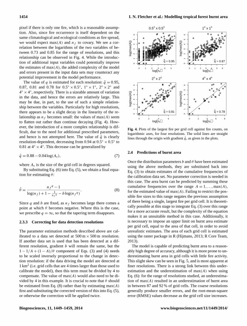
By plotting the fitted values ofb for each grid cell against arange of other variables, such asnf , θ , or max(A) (the largestobserved burn scar in each cell), there is a consistent lack ofcorrelation. We have not included all of the plots mentionedabove, as this would be somewhat redundant, due to the simi-lar patterns of each one: onlyb againstnf is shown in Fig. 3.This suggests thatb is approximately constant, and can be



0 1 2 3 4 5 6

02

46

8Cumulative frequencies

log(A)

log(

n X≥A

)

●

●●

●●

●●

●●●●●●●●●●●●●●●●●●●●●●●●●●●●●●●●●●●●●●●●●●●●●●●●●●●●●●●●●●●●●●●●●●●●●●●●●●●●●●●●●●●●●●●●●●●●●●●●●●●●●●●●●●●●●●●●●●●●●●●●●●●●●●●●●●●●●●●●●●●●●●●●●●●●●●●●●●●●●●●●●●●●●●●●●●●●●●●●●●●●●●●●●●●●●●●●●●●●●●●●●●●●●●●●●●●●●●●●●●●●●●●●●●●●●●●●●●●●●●●●●●●●●●●●●●●●●●●●●●●●●●●●●●●●●●●●●●●●●●●●●●●●●●●●●●●●●●●●●●●●●●●●●●●●●●●●●●●●●●●●●●●●●●●●●●●●●●●●●●●●●●●●●●●●●●●●●●●●●●●●●●●●●●●●●●●●●●●●●●●●●●●●●●●●●●●●●●●●●●●●●●●●●●●●●●●●●●●●●●●●●●●●●●●●●●●●●●●●●●●●●●●●●●●●●●●●●●●●●●●●●●●●●●●●●●●●●●●●●●●●●●●●●●●●●●●●●●●●●●●●●●●●●●●●●●●●●●●●●●●●●●●●●●●●●●●●●●

●

ObservedFitted

b=1.364, sd = 0.003θ = 299.6, sd = 0.000056

0 1 2 3 4 5 6

02

46

8

Frequencies

log(A)lo

g(n X

=A)

●

●

●

●

●●

●●

●●●●●●●●●●●●●

●●●●●●●●●●●●●●●●●●●●●●●●●●●●●●●●●●

●

●●●

●

●

●●●●●●●●●

●

●●

●

●

●●

●

●●●

●

●●●●●●●●●●●●●●●●●●●●●●●●●●●●●●●●●●●●●●●●●●●●●●●●●●●●●●●●● ●●

0 2 4 6 8

02

46

8

Observed log(nX≥A)

Fitt

ed lo

g(n X

≥A)

0 2 4 6 8

02

46

8

Observed log(nX=A)

Fitt

ed lo

g(n X

=A)

Observed BA = 16,384 km2

Estimated BA = 15,596 km2

Fig. 2. Plots of the observed (black) and fitted (blue) cumulativefrequency distribution (top left) and non-cumulative frequency dis-tribution (top right), with the corresponding plots fitted against ob-served values (with 1 : 1 lines, bottom row). Logarithmic axes areused for all plots. The burnt area values given in the bottom-rightplot are the total observed and estimated burnt area over the wholestudy region.

estimated by taking the mean value of the observations. Al-though there is a large amount of variation inb whennf issmall, this can be attributed to the difficulties of parameterestimation when the model is fitted to a small number of datapoints.

There appears to be a slight effect of resolution on themean value ofb per grid cell. The coarser the resolution,the larger the value of̄b is. This is further supported by thesignificantly higher value ofb obtained when the distribu-tion is fitted to the whole region. However, performing Stu-dent t tests on the estimates ofb for each pair of resolu-tions shows that there is not enough evidence at a 5 % sig-nificance level to suggest that there is a difference betweenthe means calculated here. This is true even if a one-sidedt

test is used on the estimates ofb for 0.5◦× 0.5◦ and 4◦ × 4◦,

which give the smallest and largest values ofb̄, respectively(p value = 0.2487). The mean of theb̄ across these four res-olutions is 1.27. The change in the total burnt area estimatesover the study region if a fixedb is used instead of the indi-vidual b̄ per resolution is at most 4 %. Hence, it is best forthis study to keepb = 1.27.

●

●

●

●

●●

●

●

●

●

●

●

●●

●

●●

●

●

●

●●

●

●

●

●

●

●

●●

●

●

●

●

●

●

●

●

●

●

●

●

●

●●

●

●

●

●

●

●

●

●

●

●

●●

●●

●

●

●

●

●

●

●

●

●

●●

●●

●

●

●

●●●

●

●

●

●

●

●

●

●

●

●

●

●

●

●

●

●

●●

●

●

●●●

●●

●●

●●

●

●

●●

●

●

●

●

●

●

●

●

●

●

●

●

●

●

●

●

●

●

●

●

●

●

●

●

●

●●

●

●

●

●

●

●●

●

●

●

●

●

●

●

●

●

●●

●

●

●

●

● ●

●●●

●●

●

●

●●

●

●

●●

●

●●

●

●●

●

●●●●

● ●

●

●

●

●

●

●●

●

●

●

●

●

●●

●

●

●

●

●

●

●

●●

●

●

●

●

●

●

●●

●

●

●

●

●

●

●

●

●

●

●

●

●

●

●

●●

●

●

●

●

●

●●

●

●

●●

●

●

●

●

●

●

●

●

●●

●●

●

●●

●●

●●

●

●

●●

●

●

●

●

●

●

●

●

●

●●

●●

●

●

● ●

●

●●

●

●

●

●

●

●

●

●

●

●

●

●

●

●

●

●

●

●

●●

●●

●

●

●

●

●

●●

●●

●

●

●

●

●

●

●

●

●

●

●

●

●

●

●

●

●

●

●

●

●● ●

●

●●

●

●

●

●●

●

●

●

●●

●

●

●

●

●●

●

●

●

●

●●●

●

●

●

●●

●

●

●

●

●

●

●

●

●

●

●

●

●

●

●

●

●

●

●

●

●

●

●

●●

●

●

●●

●

●●

●

●

●

●

●

●

●

●

●●

●

●

●

●●

●

●

●

0 50 100 150 200 250

0.0

0.5

1.0

1.5

2.0

2.5

3.0

0.5o x 0.5o

nf

b

b̂ = 1.246

●●

●

●

●●

●

●

●

●

●

●

●●

●

●

●

●

●●●

●

●

●

●

●

●

●

●

●

●

●

● ●

●

●

●

●●

●

●●

●

●

●

●

●

●

●

●

●

●

●

● ●

●

●

●

●●

●

●●

●●

●

●●

●●

●

●

●

●

●

●●

●

●

●

●

●

●

●

●

●

●

●

●

●

●

●●

●

●

●

●

●

●●

●

●

●

● ●●

●

●

●

●●

●●

●●●

●

●

●

●

●

●●

●●

●

●

●

●

●

●

●

●

●

●

●

●

●

●

●

●

●

●

●●

●

●

●

●

●

●

●

●

●

●

●

●

●

●

●

●

●

●

●

●●●

●

●

●

●

●

●

●

●

●

●

●

●

●

0 100 200 300 400 500 600

0.0

0.5

1.0

1.5

2.0

2.5

3.0

1o x 1o

nf

b

b̂ = 1.261

●

●●

●

●

●

●

●

●

●

●

●●

●

●

●

●●

●

●

●●

●

●

●

●●

●

●●

●

●

●

●

●

●

●

●

●

●

●

●

●

●

●

●

●

●

●●

●●

●

●●

●

●

●

●●

●

●

●

●

●●

●

●●

0 200 400 600 800 1200

0.0

0.5

1.0

1.5

2.0

2.5

3.0

2o x 2o

nf

b

b̂ = 1.288

●

●

●

●

●●

●●

●●

●

●

●

●

●

●

●●

●

●

●

●

●●●●

0 500 1000 2000 3000

0.0

0.5

1.0

1.5

2.0

2.5

3.0

4o x 4o

nf

b

b̂ = 1.293

Fig. 3. Plots of estimated values of parameterb against fire counts,nf , for all four resolutions. The solid lines horizontal lines are atb = b̄ for the values of̄b shown on each plot.

2.3.2 Estimating tapering parameterθ

We assume that there is always one single largest fire ineach grid cell, sonX≥max(A) = 1. By settingA = max(A) inEq. (4) and rearranging, we get the following approximationof θ :

θ̂ =max(A) − 1

log(nf ) + 1−1

max(A)− b log(max(A))

. (5)

Sinceb̂ = 1.27 from Sect. 2.3.1 andnf is an input vari-able, if a method of estimating max(A) is found, thenθ canbe calculated directly from Eq. (5).

The maximum size a fire can take in a grid cell is depen-dent on many factors. From a purely statistical viewpoint,the more fires in a cell, the larger max(A) is likely to be.The value of max(A) also depends on local climatic and eco-logical conditions. For example, fragmented fuel or a highfuel moisture content can severely limit fire spread, whilehigh winds and a high litter load encourage fire propagation.Additionally, the largest potential fire size is not necessarilysimilar to the actual achieved max(A), which makes this adifficult value to predict.

The estimate used in this model is simple: it is a log-linearfunction of fire counts, as described by Eq. (6):

log(max(A)) ≈ q log(nf ). (6)

This obviously takes the statistical likelihood of large firesgiven the sample size into account, and restricts max(A) to 1



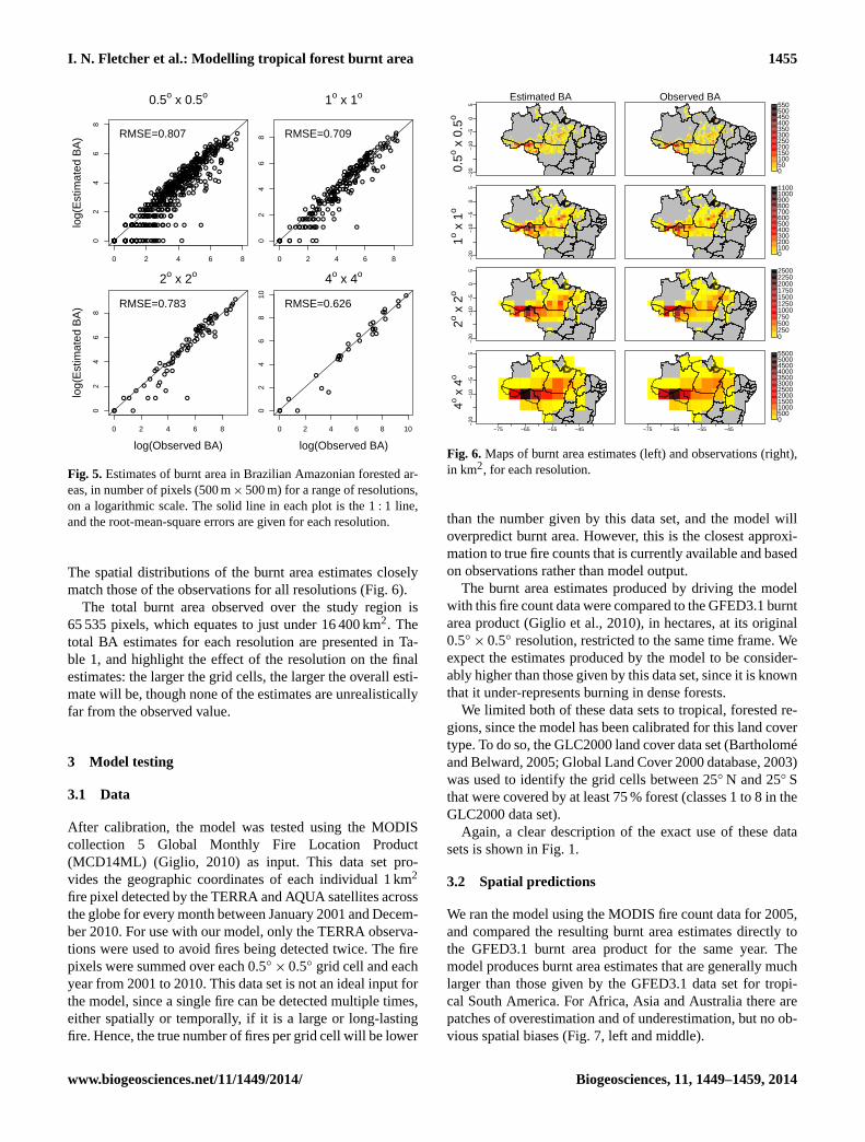
pixel if there is only one fire, which is a reasonable assump-tion. Also, since fire occurrence is itself dependent on thesame climatological and ecological conditions as fire spread,we would expect max(A) andnf to covary. We see a cor-relation between the logarithms of the two variables of be-tween 0.73 and 0.85 for the range of resolutions, and thisrelationship can be observed in Fig. 4. While the introduc-tion of additional input variables could potentially improvethe estimates of max(A), the added complexity of the modeland errors present in the input data sets may counteract anypotential improvement in the model performance.

The value ofq is estimated for each resolution:q̂ = 0.95,0.87, 0.81 and 0.78 for 0.5◦

× 0.5◦, 1◦× 1◦, 2◦

× 2◦ and4◦

× 4◦, respectively. There is a sizeable amount of variationin the data, and hence the errors are relatively large. Thismay be due, in part, to the use of such a simple relation-ship between the variables. Particularly for high resolutions,there appears to be a slight decay in the linearity of the re-lationship asnf becomes small: the values of max(A) seemto flatten out rather than continue decaying (Fig. 4). How-ever, the introduction of a more complex relationship is dif-ficult, due to the need for additional prescribed parameters,and hence is not attempted here. The value ofq̂ is clearlyresolution-dependent, decreasing from 0.94 at 0.5◦

× 0.5◦ to0.81 at 4◦ × 4◦. This decrease can be generalized by

q̂ = 0.88− 0.04log(Ac), (7)

whereAc is the size of the grid cell in degrees squared.By substituting Eq. (6) into Eq. (5), we obtain a final equa-

tion for estimatingθ :

θ̂ =nf

q− 1

log(nf ) + 1−1

nfq − b log(nf

q). (8)

Sinceq andb are fixed, asnf becomes large there comes apoint at whichθ becomes negative. Where this is the case,we prescribeq = ∞, so that the tapering term disappears.

2.3.3 Correcting for data detection resolutions

The parameter estimation methods described above are cal-ibrated to a data set detected at 500 m× 500 m resolution.If another data set is used that has been detected at a dif-ferent resolution, gradientb will remain the same, but the1− 1/A + (1− A)/θ component of Eqs. (3) and (4) needsto be scaled inversely proportional to the change in detec-tion resolution: if the data driving the model are detected at1 km2 (i.e. grid cells that are 4 times larger than those used tocalibrate the model), then this term must be divided by 4 tocompensate. The value of max(A) would also need to be di-vided by 4 in this example. It is crucial to note thatθ shouldbe estimated from Eq. (8) rather than by estimating max(A)

first and substituting the corrected version of this into Eq. (5),or otherwise the correction will be applied twice.

●

●

●

●●

● ●

●

●

●

●

●

●

●●

●●

● ●

●

●

●

●

●

●●

●●

●

●

●

●

●

●

●

●

●

●

●

●

●

●

● ●

●

●

●●

●

●

●

●

●●

●

●

●

●

●

●

●

●

●

●

●

●

●

●

●

●

●●

●

●

●

●

●

●

●

●●

●●●

●

●

●

●

●●

●

●

●

●

●

●●

●

●●

●●

●

●

●

●

●

●

●

●

●

●●●

●●

●

●●

●

●

●

●

●

●

●

● ●

●

●

●●

●

●

●

●

●●

●●

●●

●

●

●

●

● ●

●

●

●● ●

●

●

●

●

●

●

●

●

●

●

●

●

●

●

●

●

●

●

●

●

●

●

●●

●

●

●●

●

●

●

●

●

●

●

●

●

●●

●

●

●

●

●

●

●

●

●

●

●

●

●

●

●

●

● ● ●

●

●

●

●

●

●

●

●

●●

● ●

●

●

●

●

●●

●●

●

●

●

●

●

●

●

●

●

●●

●

●●

●

●●

●

● ●

●

●

●

●

●

●●

●●●

●

●

●

●

● ●

●

●●

● ●

●

●

●

●

●

●

●●

●

●

●

●

●

●

●

●

● ●

●

●

●

●●

●

●

●

●

●

●

●

●

●

●●

●

●

●

●●

●

●

●●

●

●

● ●

● ●●

●

●

●

●

●●

●

●

●

●

● ●●

●

●●

●

●●

●

●

●

●

●

●

●

●

●

●

●

●

●●

●

●

●

●

●

●

●

●●

●

●

●

●

●

●

●

●●

●

●

●

●

●

●

●

●

● ●

●

●

●

●

●

●

●●● ●

●

●

●

●

●

●

●●

●●●

●

●

●

●

●

●●

●

●

●

●

●

●

●●

●

●

●●

●

●●●

●

●

●

●

●

●

●

●●

●

●●

●

●

●

●

●

●

●

●

●

●

● ●

●

●

●

●

●

●

●

●

●●

●

●

●

● ●●

●

●

●

●

●

●●

●

●

●

●

●

●

●

●

●

●

●

●

●

●

●

●

●

●

●●

●

●

●

●

●

●

●

●

●

●

●●

●

●

●

●

●

●●●●●

●●

●●

●●

●

●

●

●

●

●

●

0 1 2 3 4 5

01

23

45

6

0.5o x 0.5o

log(nf)

log(

max

(A))

q̂ = 0.95●

●

●

●

●

●●

●

●

●

●

●

●

●

●

●

●

●

●

●

●

●

● ●

●

●

●

●

●

●

●

●

●

●

●

●

●

●

●

●

●

●

●

●●●

●●

●

●●

●

●

●

●

●

●

●

●

●

● ●

●

●

●

●

●

●

●

●

●●●

●

●●

●

●

●

●● ● ●

●●● ●

●

●

●●

● ●●

●

●

●

●

●

●

●

●

●●

●

●

●●

●

●

●

●

● ●●

●

●

●

●

●

●

●

●●

● ●

●

●

●

●

●●●

●

●●

●

●●●

● ●

●●

●●●

●●

●●

●

●

●

●

●

●

●

●

●

●

●

●

●

●

●

●

●

●

●

●

●

●

●

●

●

●

●

●

●

●●

●

●

●

●

●

●

●

●

●

●

●

●●

●●

●●

●

●

●●

●

●

0 1 2 3 4 5 6

01

23

45

6

1o x 1o

log(nf)

log(

max

(A))

q̂ = 0.87

●

●

●

●

●

●

●

●

●

●

●

●

●

●●

●

●

●●

●

●

●

●

●

●

●

●

●

●

●

●

●

●

●●

●●

●

●●

● ●

●

●●

●

●

●

●● ●

● ●

●

●

●

●

●

●

●

●

●

●

●

●

●

●

●

●

●

●

●

●

●

●

0 2 4 6

01

23

45

6

2o x 2o

log(nf)

log(

max

(A))

q̂ = 0.81●

●

●●

●

●

●

●

●

●

●

●

●

●●●

●

●

●

●

●

●

●

●

●

●

●●

●

●

0 2 4 6 8

01

23

45

6

4o x 4o

log(nf)

log(

max

(A))

q̂ = 0.78

Fig. 4. Plots of the largest fire per grid cell against fire counts, onlogarithmic axes, for four resolutions. The solid lines are straightlines through the origin with gradientq̂, as given in the plots.

2.4 Predictions of burnt area

Once the distribution parametersb andθ have been estimatedusing the above methods, they are substituted back intoEq. (3) to obtain estimates of the cumulative frequencies ofthe calibration data set. No parameter correction is needed inthis case. The area burnt can be predicted by summing thesecumulative frequencies over the rangeA = 1, . . .,max(A),for the estimated value of max(A). Failing to restrict the pos-sible fire sizes to this range negates the previous assumptionof there being a single, largest fire per grid cell. It is theoreti-cally possible at this stage to integrate Eq. (3) over this rangefor a more accurate result, but the complexity of the equationmakes it an unsuitable method in this case. Additionally, itis necessary to impose an upper limit on burnt area estimateper grid cell, equal to the area of that cell, in order to avoidunrealistic estimates. The area of each grid cell is estimatedusing the raster package in R (Hijmans, 2013; R Core Team,2013).

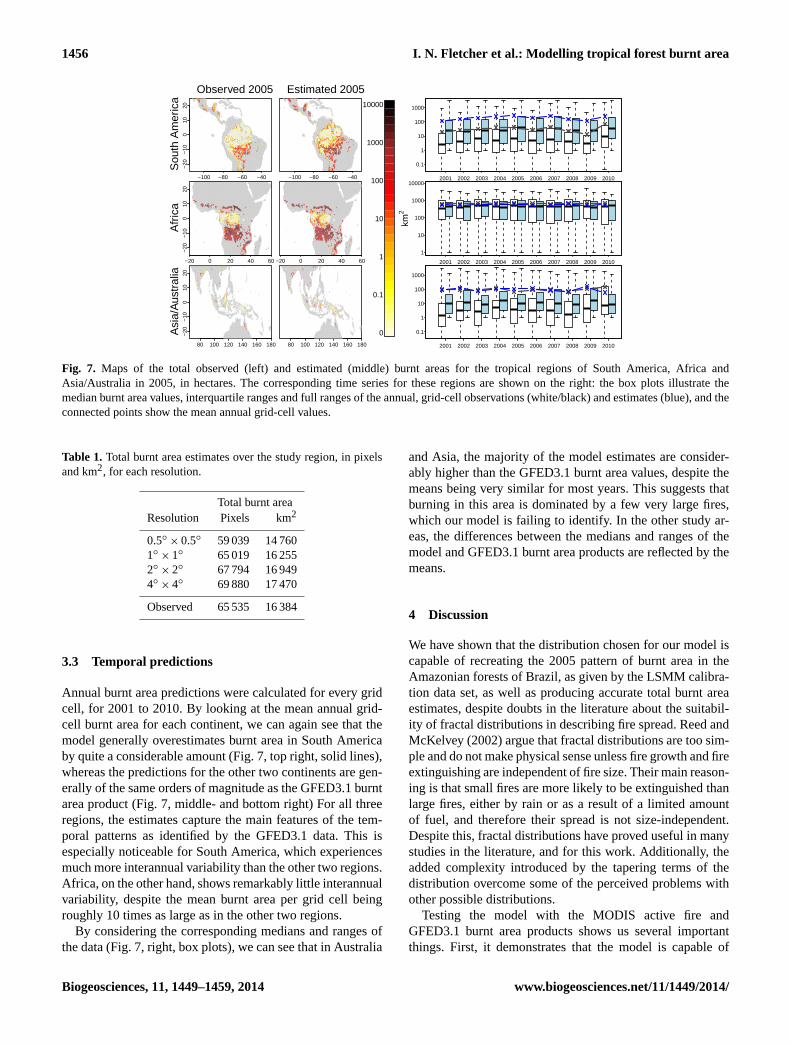
The model is capable of predicting burnt area to a reason-ably high degree of accuracy, although it is more prone to un-derestimating burnt area in grid cells with little fire activity.This slight skew can be seen in Fig. 5, and is most apparent atfiner resolutions. There is a strong link between this under-estimation and the underestimation of max(A) when usingEq. (6): for the range of resolutions studied, an underestima-tion of max(A) resulted in an underestimation of burnt areain between 87 and 92 % of grid cells. The coarse resolutionsgenerally produce smaller errors, and the root-mean-squareerror (RMSE) values decrease as the grid cell size increases.



●

●●

●

●

●

●

●

●

●

●

●●

●

●●

●

●●

●

●

●

●

●●

●

●

●

●

●●

●

●

●

●

●

●

●●

●

●

●

●

●

●

●

●

●●

●

●●

●

● ● ●

●

●●

●

●

●

● ●

●

●

●

●

●

●

●

●

●

●

●

●

●

●

●

●

●

●

●●

●

●

●

● ●

●

●●

●

●●●

●

●●

●

●

●●

●

●

●

●●

●

●

●●

●

●

●

●●

●

●●

●

●

●

●●

●

●

●●

●

●

● ●●●

●

●

●

●

●●

●

●●

●●

●

●

●

●

●

●

●

●

●

●●

●

●

●

●

●

● ●

●●

●●

●●

●●

●

●●

●

●

●

●●

●

●

●

●

●

●●

●

●●

●●

●

●

●

●

●

●

●

● ●

● ●

●

●

●●

●

●●

●

●

●

●●

● ●●

●

●

●

●

●

●

●

●

●

●●

●

●

●

●

●

●

●

●

●

●

●●

●

●

●●

●

●

●

●

●

●●

●

●

●

●

●

●

●

●

●

●

●●

●

●

●

●

●

●

●

●

●

●

●●

●

●

●

●

●●

●

●

●

●

●●

●

●

●

●●

●●

●

●

●●

●

●

●

●

●

●

●

●

●

●

●

●

●●

●

●

●

●●

●

●

●

●

● ●●

●

●

●

●

●

● ●

●

●

●

●

● ●

●

●

●

●

●

●

●●

●

●

●

●●

●

●

●

●

●

●

●

●●

●

●●

●

●

●

●

●

●

●●

●

●

●

●

●

●

●●

● ●

●

●

●

●

● ●

●

●

●

●●●●

●

●

●

●

●

●

●

●

●

●

●

●

●

●

●●

●

●●

●●

●

●

●

●● ●

●●

●

●

●

●

●●

●

●

●

●

●

●

●

●

●

●

●

●

●

●

●

●

●

●

●●

●

●

●

●

●

●

●

●●

●

●

●

● ●

● ●

●●

●

●●

●

●●

●

●

●

●

●

●

●

●

●

●

●

●

●

●●

●

●

●

●

●●

●

●

●●

●

●●

● ●

●● ●

●

●

●

●

●

●

●

●●

●

●●●●

●

●

●

●● ●

●

● ●

0 2 4 6 8

02

46

80.5o x 0.5o

log(

Est

imat

ed B

A) RMSE=0.807

●

●

●●

●

●●

●

●

●●

●

●

●

●

●

●

●

●

●

●●

●

●

●●

●

●

● ●

●

●

●● ●

●

●

●●

●

●

●●

●

●

●

●●

●

●

●

●

●

●●

●

●●

●

●

●●

●

●

●●

●

●

●

●●

●●

●●●

●

●

●●●

●

●●

●●

●

●

●

●

●

●●●

●

●

●●

●

●

●

●

●

●

●

●

●

●

●

●

●

●

●

●

●

●

●

●

●

●

●

●

●

●

●

●●

●

●

●

●

●

●

●

●

●

●

●

●

●

●

●

●

●

●

●

●

●●

●●

●

●

●

●

●

●

●●

●●

●

●

●

●

●

●●

●

●

●●

●●●

●

●

●●

●

●

●

●

●●

●

●

●

●

●

●

●

●

●●

●

●

●● ●

●

●

●

● ●

0 2 4 6 80

24

68

1o x 1o

RMSE=0.709

●

●●

●

●● ●

●

●

●

●

●

●

●●●

●● ●

●

●

●

●

●●

●

●

●●●

●

●

●

●

●

●

●

●

●

●

●

●

●

●

●

●●

●

●

●

●

●

●●

●●

●

●●

●

●●

●

●

●

●

●

●

●

●

●

●

●

●

●

0 2 4 6 8

02

46

8

2o x 2o

log(Observed BA)

log(

Est

imat

ed B

A) RMSE=0.783

●

●●

●

●

●

●

●

●

●

●●

●

●●

●

●

●

●

●

●

●

●

●

●

●

●

●

●

●

0 2 4 6 8 10

02

46

810

4o x 4o

log(Observed BA)

RMSE=0.626

Fig. 5. Estimates of burnt area in Brazilian Amazonian forested ar-eas, in number of pixels (500 m× 500 m) for a range of resolutions,on a logarithmic scale. The solid line in each plot is the 1: 1 line,and the root-mean-square errors are given for each resolution.

The spatial distributions of the burnt area estimates closelymatch those of the observations for all resolutions (Fig. 6).

The total burnt area observed over the study region is65 535 pixels, which equates to just under 16 400 km2. Thetotal BA estimates for each resolution are presented in Ta-ble 1, and highlight the effect of the resolution on the finalestimates: the larger the grid cells, the larger the overall esti-mate will be, though none of the estimates are unrealisticallyfar from the observed value.

3 Model testing

3.1 Data

After calibration, the model was tested using the MODIScollection 5 Global Monthly Fire Location Product(MCD14ML) (Giglio, 2010) as input. This data set pro-vides the geographic coordinates of each individual 1 km2

fire pixel detected by the TERRA and AQUA satellites acrossthe globe for every month between January 2001 and Decem-ber 2010. For use with our model, only the TERRA observa-tions were used to avoid fires being detected twice. The firepixels were summed over each 0.5◦

× 0.5◦ grid cell and eachyear from 2001 to 2010. This data set is not an ideal input forthe model, since a single fire can be detected multiple times,either spatially or temporally, if it is a large or long-lastingfire. Hence, the true number of fires per grid cell will be lower

Estimated BA Observed BA

0.5o x

0.5

o

−20

−10

−5

05

1o x 1

o

−20

−10

−5

05

2o x 2

o

−20

−10

−5

05

4o x 4

o

−75 −65 −55 −45

−20

−10

−5

05

−75 −65 −55 −45

050100150200250300350400450500550

010020030040050060070080090010001100

02505007501000125015001750200022502500

05001000150020002500300035004000450050005500

Fig. 6. Maps of burnt area estimates (left) and observations (right),in km2, for each resolution.

than the number given by this data set, and the model willoverpredict burnt area. However, this is the closest approxi-mation to true fire counts that is currently available and basedon observations rather than model output.

The burnt area estimates produced by driving the modelwith this fire count data were compared to the GFED3.1 burntarea product (Giglio et al., 2010), in hectares, at its original0.5◦

× 0.5◦ resolution, restricted to the same time frame. Weexpect the estimates produced by the model to be consider-ably higher than those given by this data set, since it is knownthat it under-represents burning in dense forests.

We limited both of these data sets to tropical, forested re-gions, since the model has been calibrated for this land covertype. To do so, the GLC2000 land cover data set (Bartholoméand Belward, 2005; Global Land Cover 2000 database, 2003)was used to identify the grid cells between 25◦ N and 25◦ Sthat were covered by at least 75 % forest (classes 1 to 8 in theGLC2000 data set).

Again, a clear description of the exact use of these datasets is shown in Fig. 1.

3.2 Spatial predictions

We ran the model using the MODIS fire count data for 2005,and compared the resulting burnt area estimates directly tothe GFED3.1 burnt area product for the same year. Themodel produces burnt area estimates that are generally muchlarger than those given by the GFED3.1 data set for tropi-cal South America. For Africa, Asia and Australia there arepatches of overestimation and of underestimation, but no ob-vious spatial biases (Fig. 7, left and middle).



S

outh

Am

eric

a

Afr

ica

A

sia/

Aus

tral

ia

Observed 2005

−100 −80 −60 −40−

20−

100

1020

−20 0 20 40 60

−20

−10

010

20

80 100 120 140 160 180

−20

−10

010

20

Estimated 2005

−100 −80 −60 −40

−20 0 20 40 60

80 100 120 140 160 180

0

0.1

1

10

100

1000

10000

2001 2002 2003 2004 2005 2006 2007 2008 2009 2010

0.1

1

10

100

1000

2001 2002 2003 2004 2005 2006 2007 2008 2009 2010

1

10

100

1000

10000

km2

2001 2002 2003 2004 2005 2006 2007 2008 2009 2010

0.1

1

10

100

1000

Fig. 7. Maps of the total observed (left) and estimated (middle) burnt areas for the tropical regions of South America, Africa andAsia/Australia in 2005, in hectares. The corresponding time series for these regions are shown on the right: the box plots illustrate themedian burnt area values, interquartile ranges and full ranges of the annual, grid-cell observations (white/black) and estimates (blue), and theconnected points show the mean annual grid-cell values.

Table 1. Total burnt area estimates over the study region, in pixelsand km2, for each resolution.

Total burnt areaResolution Pixels km2

0.5◦ × 0.5◦ 59 039 14 7601◦

× 1◦ 65 019 16 2552◦

× 2◦ 67 794 16 9494◦

× 4◦ 69 880 17 470

Observed 65 535 16 384

3.3 Temporal predictions

Annual burnt area predictions were calculated for every gridcell, for 2001 to 2010. By looking at the mean annual grid-cell burnt area for each continent, we can again see that themodel generally overestimates burnt area in South Americaby quite a considerable amount (Fig. 7, top right, solid lines),whereas the predictions for the other two continents are gen-erally of the same orders of magnitude as the GFED3.1 burntarea product (Fig. 7, middle- and bottom right) For all threeregions, the estimates capture the main features of the tem-poral patterns as identified by the GFED3.1 data. This isespecially noticeable for South America, which experiencesmuch more interannual variability than the other two regions.Africa, on the other hand, shows remarkably little interannualvariability, despite the mean burnt area per grid cell beingroughly 10 times as large as in the other two regions.

By considering the corresponding medians and ranges ofthe data (Fig. 7, right, box plots), we can see that in Australia

and Asia, the majority of the model estimates are consider-ably higher than the GFED3.1 burnt area values, despite themeans being very similar for most years. This suggests thatburning in this area is dominated by a few very large fires,which our model is failing to identify. In the other study ar-eas, the differences between the medians and ranges of themodel and GFED3.1 burnt area products are reflected by themeans.

4 Discussion

We have shown that the distribution chosen for our model iscapable of recreating the 2005 pattern of burnt area in theAmazonian forests of Brazil, as given by the LSMM calibra-tion data set, as well as producing accurate total burnt areaestimates, despite doubts in the literature about the suitabil-ity of fractal distributions in describing fire spread.Reed andMcKelvey(2002) argue that fractal distributions are too sim-ple and do not make physical sense unless fire growth and fireextinguishing are independent of fire size. Their main reason-ing is that small fires are more likely to be extinguished thanlarge fires, either by rain or as a result of a limited amountof fuel, and therefore their spread is not size-independent.Despite this, fractal distributions have proved useful in manystudies in the literature, and for this work. Additionally, theadded complexity introduced by the tapering terms of thedistribution overcome some of the perceived problems withother possible distributions.

Testing the model with the MODIS active fire andGFED3.1 burnt area products shows us several importantthings. First, it demonstrates that the model is capable of



producing the expected spatial patterns and temporal trendsof burning. For South America, the peaks in burning in 2005,2007 and 2010 (Aragão et al., 2007; Chen et al., 2013; Zenget al., 2008) are correctly identified. Tropical Africa, Aus-tralia and Asia show much less interannual variability, butnonetheless, the model successfully recreates the temporalpatterns. This confirms the hypothesis that active fire is suffi-cient as an input variable, and the introduction of other inputsis not necessary, although it may be useful in future modeldevelopment, especially if the model were to be extrapolatedto different biomes with considerably different climates andvegetation. It could be argued that, since burnt area and activefire are strongly correlated, the intermediate steps of calculat-ing model parameters and estimating the largest fire per gridcell are unnecessary: while it is true that rough estimates ofburnt area can be produced as a simple linear or log-linearfunction of active fire, there is a considerable amount of vari-ation in the data which would not be captured, but is byour model. A simple log-linear relationship can produce es-timates with RMSEs that are approximately twice as large asthose predicted by the model. Our model may be of less ben-efit in other regions, such as savannahs, where the correlationbetween active fires and burnt area is larger (Randerson et al.,2012).

The second interesting point of discussion resulting fromSect. 3 is that of the magnitude of burnt area predictions. Wesee in Fig. 7 that the model produces burnt area estimates thatare considerably higher than their GFED3.1 counterparts inSouth America. This is expected because the burn scar dataset used to calibrate the model was specifically designed toinclude understory fires, which are hard to detect in denseforest. For these reasons we would expect a slight overesti-mation in the other two regions tested as well, but the burntarea predictions for Asia and Australia are very close to theGFED3.1 values, and in Africa, the model actually under-estimates burnt area with respect to GFED3.1, albeit onlyslightly. Although this may be due in part to more accuratepredictions from the GFED3.1 product for these regions, it islikely that the model parameters need to be recalibrated forthese regions, as some of the modelling assumptions may nothold outside of Brazilian Amazonia.

Although it would be difficult to calibrate the model toanother region without extensive fire size data for the de-sired region, there are three points at which the distributionis likely to change. First, the underlying distribution gradient,b, is assumed to vary based on land cover type, but may alsovary due to other local variables, such as mean local tempera-ture or precipitation, or human activity. Second, the relation-ship between fire counts and the largest fire per grid cell mayalso vary from region to region, based on the same factors.Third, the small-fire taper currently has a prescribed numer-ator of 1, but there is no reason why this might not change.If this tail is solely due to issues with the resolution at whichfires are detected, as currently presumed, then theoreticallythis should not be difficult to account for.

The choice of parameter estimation methods was not with-out its difficulties. We feel that the final options used are ca-pable of producing decent burnt area estimates, and have rea-sonable physical interpretations. Parameterb represents thegradient of the distribution, i.e. the underlying rate of decayof fire sizes. We are assuming that this is predominantly de-pendent on land cover, and since we are only consideringtropical forests, there is no reason to allowb to vary. Thisdoes not mean that the rate of decay is fixed across all gridcells, since the value ofθ can have a large effect on the gra-dient of the distribution at a given fire size. Hence, whereasb represents the general land-cover-dependent decay of firesize frequencies,θ represents the specific grid cell decay.

As mentioned in Sect. 2.3.2, it is possible that the methodfor estimatingθ could be improved upon by including clima-tological input variables in the estimation of max(A), suchas precipitation or temperature. This is something that wouldbe interesting to look into further at a later stage, but is be-yond the scope of this study. As it stands,θ takes the effect ofclimate into account implicitly, since fire counts are heavilyinfluenced by climate, andnf is used in the prediction ofθ .Additionally, if Eq. (6) could be modified to be non-linear,therefore removing the slight skew of the data for low valuesof nf , the propensity of the model to underestimate smallburnt areas might also be reduced.

The purpose of this model is for it to be incorporated intoa DGVM. We will be able to use modelled fire counts in-stead of active fire pixel data as an input, and as a result itshould be possible to identify how much of the differencebetween modelled and observed burnt area seen in Sect. 3is due to the under-representation of fires in the GFED3.1product. The model will then also be comparable to existing,process-based fire models: the effect of replacing the existingrate-of-spread equations with this distribution on trace gasemissions and vegetation structure will be easy to quantify.

5 Conclusions

We have shown the main hypothesis presented in the Intro-duction to be true; it is possible to use the theory of scale in-variance to calibrate a burnt area model with only fire countsas input, as well as accurately reproduce the observed pat-tern of burn scars in the forests of Brazilian Amazonia in2005. The model can be extended, with a few modifications,to forests across the tropical latitudes, and fully captures tem-poral variability in burning. The total, annual burnt area pre-dictions are difficult to compare, due to the lack of a com-pletely suitable input data set. The accuracy and adaptabilityof the model to other ecosystems and non-tropical regions issomething that remains to be tested further.

Supplementary material related to this article isavailable online athttp://www.biogeosciences.net/11/1449/2014/bg-11-1449-2014-supplement.pdf.


http://www.biogeosciences.net/11/1449/2014/bg-11-1449-2014-supplement.pdf

http://www.biogeosciences.net/11/1449/2014/bg-11-1449-2014-supplement.pdf


Acknowledgements.The authors would like to thank the Universityof Exeter, Climate Change and Sustainable Futures group, for thefirst author’s PhD studentship. L.E.O.C Aragão acknowledges thesupport of the UK Natural Environment Research Council (NERC)(grants NE/F015356/2 and NE/1018123/1) and the CNPq andCAPES for the Science without Borders programme’s fellowship.

Edited by: F. Carswell

References

Aragão, L. E. O. C., Malhi, Y., Roman-Cuesta, R. M., Saatchi, S.,Anderson, L. O., and Shimabukuro, Y. E.: Spatial patterns andfire response of recent Amazonian droughts, Geophys. Res. Lett.,34, L07701, doi:10.1029/2006GL028946, 2007.

Ball, G. H. and Hall, D. J.: ISODATA, a novel method of dataanalysis and pattern classification, Standford Research Institute,Menlo Park, California, 1965.

Bartholomé, E. and Belward, A. S.: GLC2000: a new approach toglobal land cover mapping from Earth observation data, Int. J.Remote Sens., 26, 1959–1977, 2005.

Bofetta, G., Carbone, V., Giuliani, P., Veltri, P., and Vulpiani, A.:Power laws in solar flares: self-organized criticality or turbu-lence?, Phys. Rev. Lett., 83, 4662–4665, 1999.

Booth, B. B. B., Dunstone, N. J., Halloran, P. R., Andrews, T., andBellouin, N.: Aerosols implicated as a prime driver of twentieth-century North Atlantic climate variability, Nature, 484, 228–232,2012.

Chen, Y., Velicogna, I., Famiglietti, J. S., and Randerson, J. Y.:Satellite observations of terrestrial water storage provide earlywarning information about drought and fire season severity inthe Amazon, J. Geophys. Res.-Biogeo., 118, 1–10, 2013.

Cox, P. M., Harris, P. P., Huntingford, C., Betts, R. A., Collins, M.,Jones, C. D., Jupp, T. E., Marengo, J. A., and Nobre, C. A.: In-creasing risk of Amazonian drought due to decreasing aerosolpollution, Nature, 453, 212–215, 2008.

Cui, W. and Perera, A. H.: What do we know about forest fire sizedistribution, and why is this knowledge useful for forest manage-ment?, Int. J. Wildland Fire, 17, 234–244, 2008.

Cumming, S. G.: A parametric model of the fire-size distribution,Can. J. Forest Res., 31, 1297–1303, 2001.

Giglio, L.: MODIS Collection 5 Active Fire Product User’s GuideVersion 2.4, Science Systems and Applications, Inc., Universityof Maryland, Department of Geography, 2010.

Giglio, L., Randerson, J. T., van der Werf, G. R., Kasibhatla, P. S.,Collatz, G. J., Morton, D. C., and DeFries, R. S.: Assess-ing variability and long-term trends in burned area by mergingmultiple satellite fire products, Biogeosciences, 7, 1171–1186,doi:10.5194/bg-7-1171-2010, 2010.

Global Land Cover 2000 database: European Commission, JointResearch Centre, available at:http://bioval.jrc.ec.europa.eu/products/glc2000/glc2000.php(last access: 17 November 2012),2003.

Hijmans, R. J.: raster: raster: Geographic data analysis and mod-eling. R package version 2.1-66, available at:http://CRAN.R-project.org/package=raster(last access: October 2013), 2013.

Holmes, T. P., Prestemon, J. P., Pye, J. M., Butry, D. T., Mer-cer, D. E., and Abt, K. L.: Using size-frequency distributionsto analyze fire regimes in Florida, in: Proceedings of the 22nd

Tall Timbers Fire Ecology Conference: Fire in Temperate, Bo-real, and Montane Ecosystems, edited by: Engstrom, R. T., Gal-ley, K. E. M., and de Groot, W. J., Tall Timbers Research Station,Tallahassee, FL, 88–94, 2004.

INPE (National Institute for Space Research): PRODES: Assess-ment of Deforestation in Brazilian Amazonia project, availableat:www.obt.inpe.br/prodes/index.html, last access: March 2013.

Justice, C. O., Giglio, L., Korontzi, S., Owens, J., Morisette, J.,Roy, D., Descloitres, J., Alleaume, S., Petitcolin, F., and Kauf-man, Y.: The MODIS fire products, Remote Sens. Environ., 83,244–262, 2002.

Kawakubo, F. S., Morato, R. G., and Luchiari, A.: Use of fractionimagery, segmentation and masking techniques to classify land-use and land-cover types in the Brazilian Amazon, Int. J. RemoteSens., 34, 5452–5467, 2013.

Lima, A., Shimabukuro, Y. E., Adami, M., Freitas, R. M.,Aragão, L. E., Formaggio, A. R., and Lombardi, R.: Mapea-mento de cicatrizes de queimadas na amazônia brasileira a partirde aplicação do modelo linear de mistura espectral em imagensdo sensor MODIS, Anais do XIV Simpósio Brasileiro de Senso-riamento Remoto, Natal, 5925–5932, 2009.

Malamud, B. D., Morein, G., and Turcotte, D. L.: Forest fires: anexample of self-organized critical behavior, Science, 281, 1840–1842, 1998.

Moreno, M. V., Malamud, B. D., and Chuvieco, E.: Wildfirefrequency-area statistics in spain, Procedia Environ. Sci., 7, 182–187, 2011.

Piao, S., Sitch, S., Ciais, P., Friedlingstein, P., Peylin, P., Wang, X.,Ahlström, A., Anav, A., Canadell, J. G., Cong, N., Hunting-ford, C., Jung, M., Levis, S., Levy, P. E., Li, J., Lin, X., Lo-mas, M. R., Lu, M., Luo, Y., Ma, Y., Myneni, R. B., Poulter, B.,Sun, Z., Wang, T., Viovy, N., Zaehle, S., and Zeng, N.: Eval-uation of terrestrial carbon cycle models for their response toclimate variability and to CO2 trends, Glob. Change Biol., 14,2015–2039, doi:10.1111/gcb.12187, 2013.

Prentice, I. C., Kelley, D. I., Foster, P. N., Friedlingstein, P., Har-rison, S. P., and Bartlein, P. J.: Modeling fire and the terres-trial carbon balance, Global Biogeochem. Cy., 25, GB3005,doi:10.1029/2010GB003906, 2011.

Pueyo, S.: Self-organised criticality and the response of wildlandfires to climate change, Climatic Change, 82, 131–161, 2007.

Pueyo, S., Graça, P. M. L. D. A., Barbosa, R. I., Cots, R., Car-dona, E., and Fearnside, P. M.: Testing for criticality in ecosys-tem dynamics: the case of Amazonian rainforest and savanna fire,Ecol. Lett., 13, 793–802, 2010.

Randerson, J. T., Chen, Y., van der Werf, G. R., Rogers, B. M.,and Morton, D. C.: Global burned area and biomass burn-ing emissions from small fires, J. Geophy. Res., 117, G04012,doi:10.1029/2012JG002128, 2012.

R Core Team: R: A language and environment for statistical com-puting. R Foundation for Statistical Computing, Vienna, Aus-tria, available at:http://www.R-project.org/(last access: Septem-ber 2013), 2013.

Reed, W. J. and McKelvey, K. S.: Power-law behaviour and para-metric models for the size-distribution of forest fires, Ecol.Model., 150, 239–254, 2002.

Ricotta, C., Avena, G., and Marchetti, M.: The flaming sandpile:self-organized criticality and wildfires, Ecol. Model., 119, 73–77, 1999.


http://dx.doi.org/10.1029/2006GL028946

http://dx.doi.org/10.5194/bg-7-1171-2010

http://bioval.jrc.ec.europa.eu/products/glc2000/glc2000.php

http://bioval.jrc.ec.europa.eu/products/glc2000/glc2000.php

http://CRAN.R-project.org/package=raster

http://CRAN.R-project.org/package=raster

www.obt.inpe.br/prodes/index.html

http://dx.doi.org/10.1111/gcb.12187

http://dx.doi.org/10.1029/2010GB003906

http://dx.doi.org/10.1029/2012JG002128

http://www.R-project.org/


Rothermel, R. C.: A mathematical model for predicting fire spreadin wildland fuels, Res Pap INT-115, US Department of Agricul-ture, Intermountain Forest and Range Experiment Station, Og-den, UT, 1972.

Schoenberg, F. P., Peng, R., and Woods, J.: On the distribution ofwildfire sizes, Environmetrics, 14, 583–592, 2003.

Shimabukuro, Y. E. and Smith, J. A.: The least-square mixing mod-els to generate fraction images derived from remote sensing mul-tispectral data, IEEE T. Geosci. Remote, 29, 16–20, 1991.

Shimabukuro, Y. E., Duarte, V., Arai, E., Freitas, R. M., Lima, A.,Valeriano, D. M., Brown, I. F., and Maldonado, M. L. R.: Frac-tion images derived from Terra Modis data for mapping burnt ar-eas in Brazilian Amazonia, Int. J. Remote Sens., 30, 1537–1546,2009.

Solé, R. V. and Manrubia, S. C.: Extinction and self-organized crit-icality in a model of large-scale evolution, Phys. Rev. E, 54, 42–45, 1996.

Sornette, A. and Sornette, D.: Self-organized criticality and earth-quakes, Europhys. Lett., 9, 197–202, 1989.

Thonicke, K., Spessa, A., Prentice, I. C., Harrison, S. P., Dong, L.,and Carmona-Moreno, C.: The influence of vegetation, firespread and fire behaviour on biomass burning and trace gas emis-sions: results from a process-based model, Biogeosciences, 7,1991–2011, doi:10.5194/bg-7-1991-2010, 2010.

van der Werf, R., Randerson, J. T., Giglio, L., Gobron, N., and Dol-man, A. J.: Climate controls on the variability of fires in thetropics and subtropics, Global Biogeochem. Cy., 22, GB3028,doi:10.1029/2007GB003122, 2008.

van der Werf, G. R., Randerson, J. T., Giglio, L., Collatz, G. J.,Mu, M., Kasibhatla, P. S., Morton, D. C., DeFries, R. S.,Jin, Y., and van Leeuwen, T. T.: Global fire emissions and thecontribution of deforestation, savanna, forest, agricultural, andpeat fires (1997–2009), Atmos. Chem. Phys., 10, 11707–11735,doi:10.5194/acp-10-11707-2010, 2010.

Zeng, N., Yoon, J. H., Marengo, J. A., Subramaniam, A., No-bre, C. A., Mariotti, A., and Neelin, J. D.: Causes and impactsof the 2005 Amazon drought, Environ. Res. Lett., 3, 014002,doi:10.1088/1748-9326/3/1/014002, 2008.


http://dx.doi.org/10.5194/bg-7-1991-2010

http://dx.doi.org/10.1029/2007GB003122

http://dx.doi.org/10.5194/acp-10-11707-2010

http://dx.doi.org/10.1088/1748-9326/3/1/014002

Documents

Fractal properties of forest fires in Amazonia as a basis for.pdf