Embed Size (px)
Citation preview
Fractal Audio Coding
by
Henry Xiao
A thesis submitted to the
School of Computing
in conformity with the requirements for
the degree of Master of Science
Queen’s University
Kingston, Ontario, Canada
July 2005
Copyright c© Henry Xiao, 2005
Abstract
We explore the performance of applying fractal coding on audio data. Some con-
ventional fractal coding problems have been studied with audio data to provide an
overview on this subject.
A review of fractal coding is presented. We implement a fractal audio coding
scheme to carry out the experiments. The performance of the scheme can be con-
trolled by a number of different parameters, including mapping tolerance, scaling
factor, partition range, domain specification, and bit allocation. Empirical results
have been obtained from experimenting on various audio data in our testing set un-
der different parameter combinations. Some conclusions and suggestions have been
made by analyzing and comparing experimental results. The study leads us to con-
clude that fractal coding is not an appropriate model to be applied alone to complex
audio data. A major barrier is the inability to represent smooth continuous functions.
With the new trend of integrating some other methods in fractal coding research,
we discuss some future aspects of fractal audio coding, and some possible improve-
ments by combining it with other techniques such as wavelet transforms.
i
Acknowledgments
I am very grateful to this experience of doing the research and writing up this thesis
which leads me into this challenging but fascinating research world. I would also take
this opportunity to thank:
• My supervisor, Dr. David Rappaport, who not only gave me the chance to be
his master student, but also trusted in me by leaving me the freedom to pursue
my research with my interests.
• My co-supervisor, Dr. Henk Meijer, who taught me to make the research life
fun, and frequently distracted me from my research with many of his fruitful
new ideas.
• School of Computing, where I found myself in the research atmosphere, and
really enjoyed to be part of it.
• My parents, without whom I would never be here, and especially my grandma,
who sacrificed so much to give me a better life.
• School of Graduate Studies&Research for awarding me scholarship which funds
my studies here.
ii
Contents
Abstract i
Acknowledgments ii
Contents iii
List of Tables v
List of Figures vi
1 Introduction 1
2 Fractal Compression 32.1 Introduction . . . . . . . . . . . . . . . . . . . . . . . . . . . . . . . . 3
2.1.1 Fractal Development . . . . . . . . . . . . . . . . . . . . . . . 42.1.2 Fractal Properties . . . . . . . . . . . . . . . . . . . . . . . . . 52.1.3 Fractal Examples . . . . . . . . . . . . . . . . . . . . . . . . . 6
2.2 Fractal Mathematical Background . . . . . . . . . . . . . . . . . . . . 82.2.1 Complete Metric Spaces . . . . . . . . . . . . . . . . . . . . . 92.2.2 Contractive Mapping Fixed-Point Theorem . . . . . . . . . . . 102.2.3 Affine Transformations . . . . . . . . . . . . . . . . . . . . . . 132.2.4 Partitioned Iterated Function Systems (PIFS) . . . . . . . . . 142.2.5 Image and Audio Models . . . . . . . . . . . . . . . . . . . . . 16
2.3 Compression and Decompression Algorithm . . . . . . . . . . . . . . 202.3.1 Fractal Encoding . . . . . . . . . . . . . . . . . . . . . . . . . 202.3.2 Fractal Decoding . . . . . . . . . . . . . . . . . . . . . . . . . 23
2.4 Advantages and Weaknesses . . . . . . . . . . . . . . . . . . . . . . . 232.5 Conclusion . . . . . . . . . . . . . . . . . . . . . . . . . . . . . . . . . 25
3 A Review of Relevant Literature 263.1 Introduction . . . . . . . . . . . . . . . . . . . . . . . . . . . . . . . . 26
iii
3.2 Fractal Coding Problems . . . . . . . . . . . . . . . . . . . . . . . . . 273.2.1 Partition Scheme . . . . . . . . . . . . . . . . . . . . . . . . . 283.2.2 Domain Pool . . . . . . . . . . . . . . . . . . . . . . . . . . . 303.2.3 Decoding . . . . . . . . . . . . . . . . . . . . . . . . . . . . . 343.2.4 Efficient Storage . . . . . . . . . . . . . . . . . . . . . . . . . 36
3.3 Hybrid Fractal Coding . . . . . . . . . . . . . . . . . . . . . . . . . . 373.3.1 DCT and Fractal Coding . . . . . . . . . . . . . . . . . . . . . 383.3.2 Wavelet and Fractal Coding . . . . . . . . . . . . . . . . . . . 39
3.4 Conclusion . . . . . . . . . . . . . . . . . . . . . . . . . . . . . . . . . 41
4 Implementation and Empirical Results 424.1 Fractal Audio with Binary Partition . . . . . . . . . . . . . . . . . . . 43
4.1.1 Encoding . . . . . . . . . . . . . . . . . . . . . . . . . . . . . 434.1.2 Decoding . . . . . . . . . . . . . . . . . . . . . . . . . . . . . 48
4.2 Testing Setups . . . . . . . . . . . . . . . . . . . . . . . . . . . . . . . 504.2.1 Testing Audio Data . . . . . . . . . . . . . . . . . . . . . . . . 504.2.2 Test Measures . . . . . . . . . . . . . . . . . . . . . . . . . . . 51
4.3 Sample Testing Results . . . . . . . . . . . . . . . . . . . . . . . . . . 524.3.1 Tolerance . . . . . . . . . . . . . . . . . . . . . . . . . . . . . 534.3.2 Scaling and Offset Bit Allocation . . . . . . . . . . . . . . . . 554.3.3 Audio Type . . . . . . . . . . . . . . . . . . . . . . . . . . . . 574.3.4 Scaling Factor . . . . . . . . . . . . . . . . . . . . . . . . . . . 594.3.5 Fractal Limitation . . . . . . . . . . . . . . . . . . . . . . . . 614.3.6 Other Issues . . . . . . . . . . . . . . . . . . . . . . . . . . . . 65
4.4 Conclusion . . . . . . . . . . . . . . . . . . . . . . . . . . . . . . . . . 66
5 Discussion 685.1 Summary and Conclusion . . . . . . . . . . . . . . . . . . . . . . . . 685.2 Recommendations for Future Work . . . . . . . . . . . . . . . . . . . 69
Bibliography 70
Appendices 73
A Testing Audio File 74
B WAVE PCM Format 76
iv
List of Tables
2.1 Fractal Encoding Mapping Example . . . . . . . . . . . . . . . . . . . 23
4.1 Fractal Audio Encoding Results . . . . . . . . . . . . . . . . . . . . . 584.2 Compression Ratio versus Scaling Factor . . . . . . . . . . . . . . . . 604.3 rms Mean versus Scaling Factor . . . . . . . . . . . . . . . . . . . . . 604.4 Silent Audio Sequence Encoding Results . . . . . . . . . . . . . . . . 614.5 White Noise Sequence Encoding Results . . . . . . . . . . . . . . . . 624.6 Sine Sequence Encoding Results . . . . . . . . . . . . . . . . . . . . . 63
v
List of Figures
2.1 Sierpinski Triangle Generating . . . . . . . . . . . . . . . . . . . . . . 62.2 Sierpinski Triangle Mapping . . . . . . . . . . . . . . . . . . . . . . . 72.3 Lena Image Fractal Encoding . . . . . . . . . . . . . . . . . . . . . . 82.4 Domain Range Mapping . . . . . . . . . . . . . . . . . . . . . . . . . 152.5 Quadtree and HV Range Partition . . . . . . . . . . . . . . . . . . . 162.6 Fractal Encoding Example . . . . . . . . . . . . . . . . . . . . . . . . 22
4.1 Classification Classes of Quadtree Partition Based Fractal Image Coding 464.2 Classification Classes of Binary Partition Based Fractal Audio Coding 474.3 Compression Ratio versus Tolerance Chart . . . . . . . . . . . . . . . 544.4 rms Mean versus Tolerance Chart . . . . . . . . . . . . . . . . . . . . 544.5 Scaling Factor Bit Allocation Chart . . . . . . . . . . . . . . . . . . . 564.6 Graphic Representation of Original and Result Sine Audio Sequences 64
B.1 8-bit and 16-bit Resolution WAVE Data Organization . . . . . . . . . 77B.2 WAVE Chunk Structure Diagram . . . . . . . . . . . . . . . . . . . . 77B.3 WAVE Chunk Specification . . . . . . . . . . . . . . . . . . . . . . . 78B.4 WAVE Audio File Example . . . . . . . . . . . . . . . . . . . . . . . 79
vi
Chapter 1
Introduction
Fractals were first introduced in the field of geometry. The birth of fractal geometry
is usually traced back to the IBM mathematician Benoit B. Mandelbrot and the 1977
publication of his book “The Fractal Geometry of Nature”. Later, Michael Barnsley,
a leading researcher from Georgia Tech, found a way of applying this idea to image
representation and compression with the mathematics of Iterated Functions Systems
(IFS). Fractal compression algorithms based on IFS are not practical because of their
high computational complexity. It is Arnode Jacquin, who finally set a practical
fractal coding algorithm using Partitioned Iterated Function Systems (PIFS). Since
the development of PIFS, fractal image coding has been widely studied and various
schemes have been derived and implemented.
Because of fractal image coding’s various shortcomings, researchers still can not
deliver a practical fractal image coding scheme. For this reason, fractal coding is
rarely studied on other types of data except on images. Recently, fractal coding has
been extended to audio data as its natural next step. Our interest in this thesis is to
explore this possibility. We will experiment on various audio data with conventional
1
CHAPTER 1. INTRODUCTION 2
fractal coding schemes to gather performance results. Then, through analyzing and
comparing the resulting data, we will attempt to understand fractal coding behaviour
on audio data, which may contribute to future research in this aspect.
The thesis is organized starting from some formal fractal theory in Chapter 2. A
brief fractal audio model is provided based on the conventional fractal image model.
The encoding and decoding algorithms are explained through examples. A review of
fractal coding researches is presented in Chapter 3. We mainly address fractal coding
and related problems from fractal image compression studies. Our implementation of
fractal audio coding and experimental results are described in Chapter 4. We provide
details of our implementation by comparing it with conventional fractal image coding
implementations. Experiments and empirical results are presented from different
perspectives. Some conclusions and suggestions are made by studying the resulting
data. Some discussion and future aspects regarding fractal audio coding and fractal
systems are proposed in the final chapter.
Chapter 2
Fractal Compression
2.1 Introduction
In this chapter, we shall first present fractal compression as it is usually presented,
without any reference to other conventional compression methods. A short mathe-
matical background of fractal compression is provided. The reader unfamiliar with
fractal compression is referred to [5] and [11] for a more detailed treatment. We
further relate fractal compression with audio data1 to present the compression and
decompression algorithms. Fractal compression advantages and weaknesses from the
previous studies on fractal image compression are presented. It is noticeable that the
compression scheme is identical on both kinds of data, thus share the same advan-
tages and suffer the same weaknesses. However, we believe the effects may vary since
our human perceptions of audio and image are very different.
1In this thesis, we use WAVE PCM format, see Appendix B on page 76
3
CHAPTER 2. FRACTAL COMPRESSION 4
2.1.1 Fractal Development
Fractals were not developed for data compression in the first place, but as a different
kind of geometry by the IBM mathematician Benoit B. Mandelbrot. In 1981, math-
ematician John Hutchinson used the theory of iterated function system to model
collections of contractive transformations in a metric space as dynamical systems,
which later provides the theoretical support of recognizing fractals in metric space.
It was Michael Barnsley, eventually, who generated the fractal model using Iterated
Function Systems (IFS), and led to encoding of images to achieve significant com-
pression.
However, Barnsley’s image compression algorithm based on fractal mathematics
was inefficient and unpractical suffering a space searching problem that was too large
to be practical. In 1988, one of Barnsley’s Ph.D. students, Arnaud Jacquin, arrived a
modified scheme for representing images called Partitioned Iterated Function Systems
(PIFS), and implemented the algorithm in his Ph.D. thesis. The basic idea of the
algorithm is to convert the whole image into PIFS. It immediately made the fractal
image compression algorithm more practical, however, by sacrificing the compression
ratio. After Jacquin’s PIFS, there were many other modified schemes [5](ch.11 and
ch.13), but none of them made any significant progress. Most of the later publications
on the subject of fractals follow the PIFS, but focus on some possible improvements.
The two big problems of Jacquin’s algorithm are the partition selection scheme for
encoding, and the speed of decoding.
Fractal compression was lately applied to audio data in [25]. The general belief
is that a purely fractal coding scheme is not suitable for audio compression. The
reason originates from the fact that fractal compression is mostly based on a fractal
CHAPTER 2. FRACTAL COMPRESSION 5
system’s ability to approximate discontinuous functions, but audio signals usually
exhibit greater smoothness than images. Regarding the remarks above, we think
that more experiments should be done with different types of audio data based on
conventional fractal coding schemes to demonstrate fractal behavior on audio data,
or simply for understanding the nature of fractals.
2.1.2 Fractal Properties
A definition of the term fractal is difficult. People usually regard fractals as a set of
properties. Fisher has given a definition of the property set in his book [5](pg.26) as
follows:
If we consider a set F to be a fractal, we think of it as having (some) ofthe following properties:
1. F has detail at every scale.
2. F is (exactly, approximately, or statistically) self-similar.
3. The “fractal dimension” of F is greater than its topological dimen-sion2.
4. There is a simple algorithm description of F .
We feel this definition of the property set is somehow hard to measure, and not
very useful for understanding fractal theory. A more useful and rigorous comparison
can be made with Vector Quantization (for details, see [6]) for the reader familiar
with conventional compression methods.
In general, the principle of mapping an n-dimensional vector to a unique symbol
from the codebook is called vector quantization. The quantization process can be
viewed as identifying patterns, and storing only a few of the common patterns to
2For details on fractal dimension and topological dimension, see [27].
CHAPTER 2. FRACTAL COMPRESSION 6
form the codebook such that the compression is achieved. The similarity to fractal
compression is apparent. The noticeable difference is that vector quantization uses
straight copy which can be lossless, but fractal encoding needs to find out the mapping
functions from the domain blocks to the range blocks3, which is a lossy scheme. More
important, fractal compression’s codebook, which is referred as a “virtual codebook”
in some contexts, is implicitly specified by a set of iteration functions. So fractal
compression in theory allows higher compression ratio, but more unpredictable than
vector quantization on the other hand.
2.1.3 Fractal Examples
We provide two fractal examples in this section for demonstration purposes.
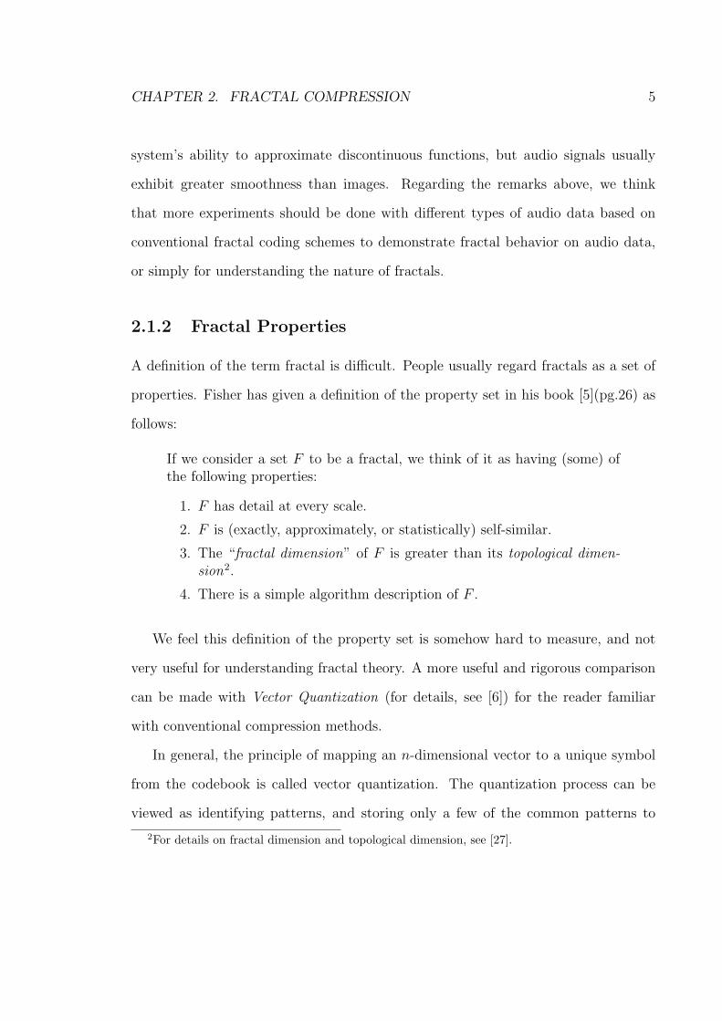
The first example is generating Sierpinski’s Triangle using an IFS. We can see
from Figure 2.1 that at each iteration, we shrink the original triangle by a factor of
2, make three copies, and place them to form a new triangle one iteration further.
(a) Initial Image (b) First Iteration (c) Fifth Iteration (d) Sixth Iteration
Figure 2.1: Sierpinski Triangle example of generating sequence from iterating.
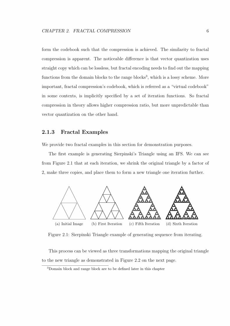
This process can be viewed as three transformations mapping the original triangle
to the new triangle as demonstrated in Figure 2.2 on the next page.
3Domain block and range block are to be defined later in this chapter
CHAPTER 2. FRACTAL COMPRESSION 7
y
x
y
x
w2
w1
w3
Figure 2.2: Sierpinski Triangle mapping from three transformations.
The mathematical expressions of the transformations are given below:
w1
(xy
)=
(1/2 00 1/2
)(xy
)(2.1)
w2
(xy
)=
(1/2 00 1/2
)(xy
)+
(1/41/2
)(2.2)
w3
(xy
)=
(1/2 00 1/2
)(xy
)+
(1/20
)(2.3)
It is important to observe that because of the resolution in Figure 2.1, there is
hardly any visible difference between the fifth and the sixth iterations. The Sier-
pinski’s triangle sequence thus visually converges to one triangle within a certain
threshold. Reversely, if we take the sequence backward, for the Sierpinski triangle
sequence, we only need to know the mapping functions (i.e., w1, w2, and w3) to get
the whole picture. This is in essence of how fractal compression works.
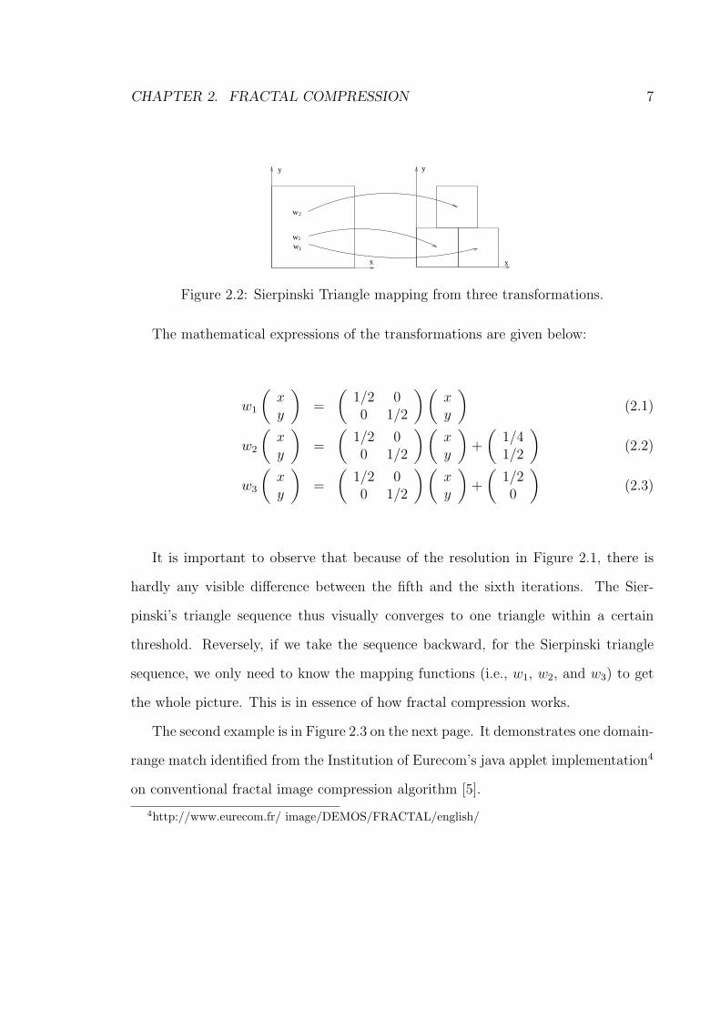
The second example is in Figure 2.3 on the next page. It demonstrates one domain-
range match identified from the Institution of Eurecom’s java applet implementation4
on conventional fractal image compression algorithm [5].
4http://www.eurecom.fr/ image/DEMOS/FRACTAL/english/

CHAPTER 2. FRACTAL COMPRESSION 8
Figure 2.3: Fractal encoding from a domain block maps to a range block on Lenaimage.
The match is calculated through the rotation and modification. And since the
domain block is twice the size of the range block in this case, the reduction is needed
afterward. Essentially, in image sense, the rotation and modification are the process
to get a proper transform function, which adjust the orientation and luminance of the
domain block. The Lena image is a widely used test figure in image compression. It
illustrates the idea that natural images have self-similarities or patterns embedded.
2.2 Fractal Mathematical Background
This section is devoted to making the above demonstrations mathematically precise.
The mathematics of fractals is related to metric spaces. However, we do not give a
concrete treatment on that subject. The interested reader is referred to [5], [11], or
any textbook on metric spaces. Fractal notions are better explained here. The image
fractal model is based on a conventional fractal image compression scheme, and the
audio fractal model is constructed based on the image fractal model.
CHAPTER 2. FRACTAL COMPRESSION 9
2.2.1 Complete Metric Spaces
We give the following definitions and theorems on the metric space related to our
subject.
Definition 1. A metric space is a set X on which a real-valued distance function
d : X ×X → R is defined, satisfying the following properties:
1. d(a, b) ≥ 0 for all a, b ∈ X.
2. d(a, b) = 0 if and only if a = b, for all a, b ∈ X.
3. d(a, b) = d(b, a) for all a, b ∈ X.
4. d(a, c) ≤ d(a, b) + d(b, c) for all a, b, c ∈ X (triangle inequality).
Such a function d is called a metric.
Definition 2. A map f : X → X is contractive over the metric space (X, d) if:
d(f(x), f(y)) ≤ s · d(x, y) ∀x, y ∈ X
where 0 ≤ s < 1 is called the contractivity of f .
Definition 3. A sequence {xn}∞n=1 in X is said to converge to some x ∈ X where
(X, d) is a metric space if ∀ε > 0 ∃N > 0 such that:
d(x, xn) < ε ∀n ≥ N .
Definition 4. A sequence {xn}∞n=1 in X is a Cauchy sequence if ∀ε > 0 ∃N > 0
such that:
d(xm, xn) < ε ∀n, m ≥ N .
CHAPTER 2. FRACTAL COMPRESSION 10
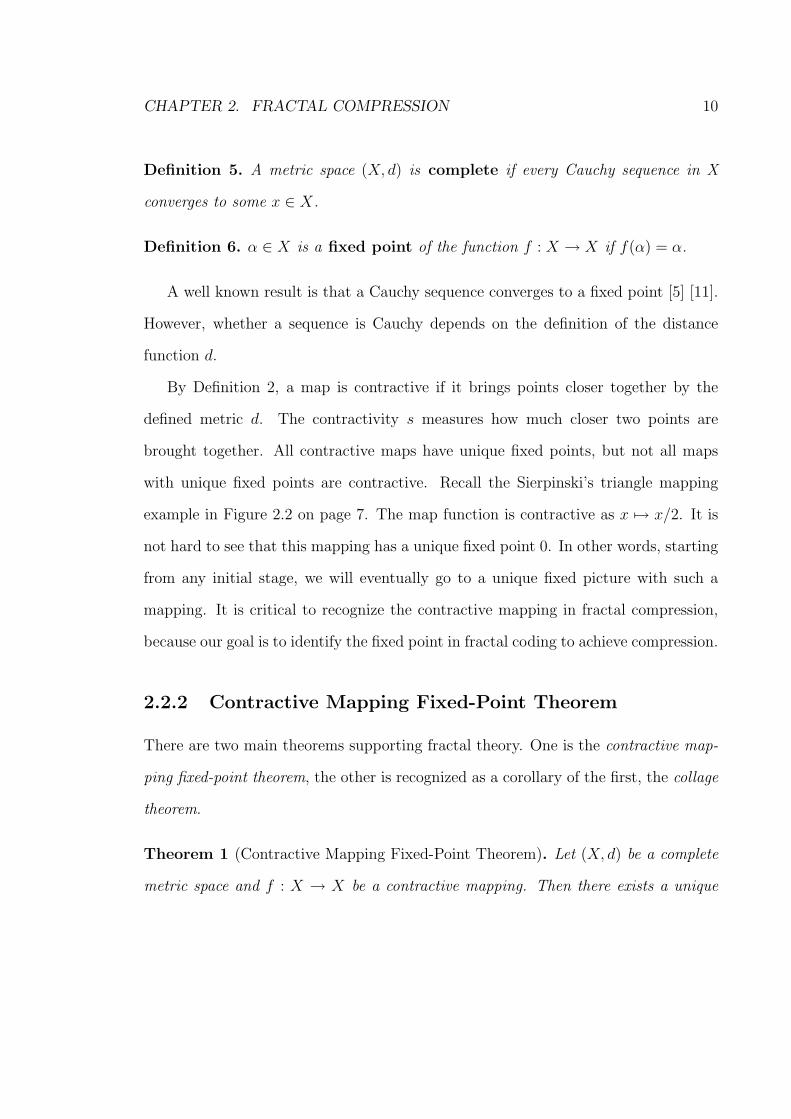
Definition 5. A metric space (X, d) is complete if every Cauchy sequence in X
converges to some x ∈ X.
Definition 6. α ∈ X is a fixed point of the function f : X → X if f(α) = α.
A well known result is that a Cauchy sequence converges to a fixed point [5] [11].
However, whether a sequence is Cauchy depends on the definition of the distance
function d.
By Definition 2, a map is contractive if it brings points closer together by the
defined metric d. The contractivity s measures how much closer two points are
brought together. All contractive maps have unique fixed points, but not all maps
with unique fixed points are contractive. Recall the Sierpinski’s triangle mapping
example in Figure 2.2 on page 7. The map function is contractive as x 7→ x/2. It is
not hard to see that this mapping has a unique fixed point 0. In other words, starting
from any initial stage, we will eventually go to a unique fixed picture with such a
mapping. It is critical to recognize the contractive mapping in fractal compression,
because our goal is to identify the fixed point in fractal coding to achieve compression.
2.2.2 Contractive Mapping Fixed-Point Theorem
There are two main theorems supporting fractal theory. One is the contractive map-
ping fixed-point theorem, the other is recognized as a corollary of the first, the collage
theorem.
Theorem 1 (Contractive Mapping Fixed-Point Theorem). Let (X, d) be a complete
metric space and f : X → X be a contractive mapping. Then there exists a unique
CHAPTER 2. FRACTAL COMPRESSION 11
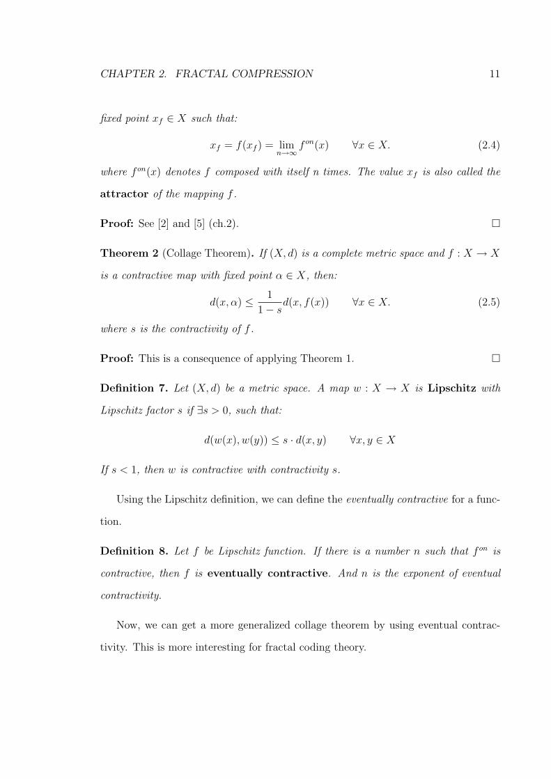
fixed point xf ∈ X such that:
xf = f(xf ) = limn→∞
f on(x) ∀x ∈ X. (2.4)
where f on(x) denotes f composed with itself n times. The value xf is also called the
attractor of the mapping f .
Proof: See [2] and [5] (ch.2). ¤
Theorem 2 (Collage Theorem). If (X, d) is a complete metric space and f : X → X
is a contractive map with fixed point α ∈ X, then:
d(x, α) ≤ 1
1− sd(x, f(x)) ∀x ∈ X. (2.5)
where s is the contractivity of f .
Proof: This is a consequence of applying Theorem 1. ¤
Definition 7. Let (X, d) be a metric space. A map w : X → X is Lipschitz with
Lipschitz factor s if ∃s > 0, such that:
d(w(x), w(y)) ≤ s · d(x, y) ∀x, y ∈ X
If s < 1, then w is contractive with contractivity s.
Using the Lipschitz definition, we can define the eventually contractive for a func-
tion.
Definition 8. Let f be Lipschitz function. If there is a number n such that f on is
contractive, then f is eventually contractive. And n is the exponent of eventual
contractivity.
Now, we can get a more generalized collage theorem by using eventual contrac-
tivity. This is more interesting for fractal coding theory.
CHAPTER 2. FRACTAL COMPRESSION 12
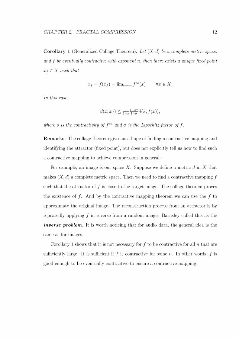
Corollary 1 (Generalized Collage Theorem). Let (X, d) be a complete metric space,
and f be eventually contractive with exponent n, then there exists a unique fixed point
xf ∈ X such that
xf = f(xf ) = limk→∞ f ok(x) ∀x ∈ X.
In this case,
d(x, xf ) ≤ 11−s
1−σn
1−σd(x, f(x)),
where s is the contractivity of f on and σ is the Lipschitz factor of f .
Remarks: The collage theorem gives us a hope of finding a contractive mapping and
identifying the attractor (fixed point), but does not explicitly tell us how to find such
a contractive mapping to achieve compression in general.
For example, an image is our space X. Suppose we define a metric d in X that
makes (X, d) a complete metric space. Then we need to find a contractive mapping f
such that the attractor of f is close to the target image. The collage theorem proves
the existence of f . And by the contractive mapping theorem we can use the f to
approximate the original image. The reconstruction process from an attractor is by
repeatedly applying f in reverse from a random image. Barnsley called this as the
inverse problem. It is worth noticing that for audio data, the general idea is the
same as for images.
Corollary 1 shows that it is not necessary for f to be contractive for all n that are
sufficiently large. It is sufficient if f is contractive for some n. In other words, f is
good enough to be eventually contractive to ensure a contractive mapping.
CHAPTER 2. FRACTAL COMPRESSION 13
2.2.3 Affine Transformations
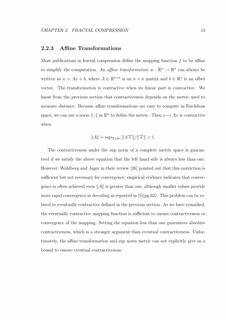
Most publications in fractal compression define the mapping function f to be affine
to simplify the computation. An affine transformation w : Rn → Rn can always be
written as w = Ax + b, where A ∈ Rn×n is an n × n matrix and b ∈ Rn is an offset
vector. The transformation is contractive when its linear part is contractive. We
know from the previous section that contractiveness depends on the metric used to
measure distance. Because affine transformations are easy to compute in Euclidean
space, we can use a norm ‖ ·‖ in Rn to define the metric. Then x 7→ Ax is contractive
when
‖A‖ = sup−→x ∈Rn ‖A−→x ‖/‖−→x ‖ < 1.
The contractiveness under the sup norm of a complete metric space is guaran-
teed if we satisfy the above equation that the left hand side is always less than one.
However, Wohlberg and Jager in their review [26] pointed out that this restriction is
sufficient but not necessary for convergence; empirical evidence indicates that conver-
gence is often achieved even ‖A‖ is greater than one, although smaller values provide
more rapid convergence in decoding as reported in [5](pg.62). This problem can be re-
lated to eventually contractive defined in the previous section. As we have remarked,
the eventually contractive mapping function is sufficient to ensure contractiveness or
convergence of the mapping. Setting the equation less than one guarantees absolute
contractiveness, which is a stronger argument than eventual contractiveness. Unfor-
tunately, the affine transformation and sup norm metric can not explicitly give us a
bound to ensure eventual contractiveness.
CHAPTER 2. FRACTAL COMPRESSION 14
2.2.4 Partitioned Iterated Function Systems (PIFS)
The Sierpinski triangle in Figure 2.1 on page 6 demonstrates the way of using IFS.
However, unlike the example, our real spaces are very irregular. In most cases, it
would be rather impossible to find such a perfect mapping for the whole space. Thus
Jacquin introduced Partitioned Iterated Function Systems (PIFS) in his work [9]. A
PIFS is a generalization of an IFS, and attempts to ease the IFS computation by
partitioning the whole space into subspaces. In other words, the PIFS is a restricted
version of the IFS.
Definition 9. Let (X, d) be a complete metric space, and let Di ⊂ X for i = 1, . . . , n,
such that⋃
i Di = X. A PIFS is a collection of contractive maps wi : Di → X, for
i = 1, . . . , n.
One problem brought up from PIFS is the partition. The space has to be par-
titioned into subspaces. It is necessary to ensure that the addition of the subspaces
covers the original space. Also, the partition scheme dominates the final map set,
which is essential to the coding process. Moreover, finding an optimal fractal encod-
ing has been shown as NP-hard [21], and collage based fractal coding may produce a
solution of arbitrary distance from the optimal solution. One partition scheme thus
can yield very unpredictable results on different spaces.
Jacquin first introduced PIFS on fractal image compression. The image space
is naturally recognized as a 2D space. The partition scheme simply partitions the
whole space twice into the range set and the domain set. Both sets cover the whole
image space, with the domain set allowing overlaps. A shortcoming of using an affine
transformation, the partition schemes for the domain set and the range set have to
give the same geometric shaped domain and range blocks, which are usually squares or
CHAPTER 2. FRACTAL COMPRESSION 15
rectangles. The domain block is set to be twice as big as the range block in Jacquin’s
original scheme [9], which is widely accepted in fractal image compression field. The
reason for allowing domain overlapping is to smooth artifacts between blocks in the
decoding process. The mappings between the domain and the range blocks are as
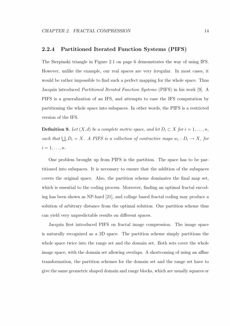
demonstrated in Figure 2.4. For each range block, we find a proper domain block to
map to. The final map set is composed of mappings for each range block from the
range set.
Range Partition Domain Partition
Figure 2.4: Mapping from the domain set to the range set.
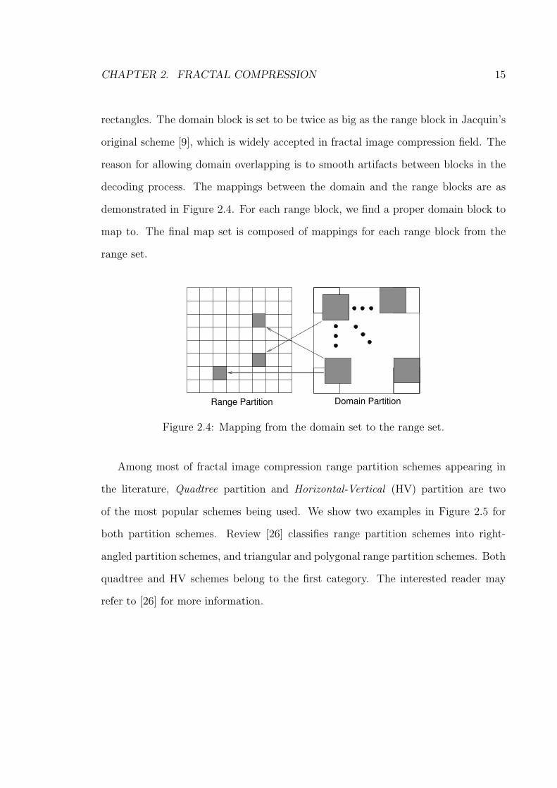
Among most of fractal image compression range partition schemes appearing in
the literature, Quadtree partition and Horizontal-Vertical (HV) partition are two
of the most popular schemes being used. We show two examples in Figure 2.5 for
both partition schemes. Review [26] classifies range partition schemes into right-
angled partition schemes, and triangular and polygonal range partition schemes. Both
quadtree and HV schemes belong to the first category. The interested reader may
refer to [26] for more information.
CHAPTER 2. FRACTAL COMPRESSION 16
(a) Quadtree range parti-tion
(b) HV range partition
Figure 2.5: Examples of quadtree and HV range partition schemes
PIFS is recognized as a significant improvement over IFS. It reduces large amount
of searching time both theoretically and practically. Furthermore, there are some
potentials to improve fractal encoding like applying different partition schemes or
taking different mapping methods. Comparing with some other advanced method of
generating fractals such as Weighted Finite Automata, PIFS also have the beauty of
simplicity. For the above reasons, our research on fractal audio coding uses PIFS in
the same way as many conventional fractal image compression schemes.
2.2.5 Image and Audio Models
Fractal image and audio models can be naturally generated from fractal theory. In
general, for a given space, we need to find a proper metric of the distance measure
to define a complete metric space. Then we need to define a PIFS in the metric
space, and the mapping method between the domain block and the range block. We
provide a fractal image model and a fractal audio model in the following contents in
this section.
CHAPTER 2. FRACTAL COMPRESSION 17
Fractal Image Model
Image space is a 2D space consisting of pixels. The location of each pixel is given by
two co-ordinates. Here, we take monochrome images. The pixel values range from 0 to
255 representing grey levels. An image containing M ×N pixels can be thought of as
a vector in an n = M ·N -dimensional space. Then the space is {0, 1, . . . , 255}n ⊂ Rn.
Common norms in Rn are the p-norms, defined by:
‖x‖p = (|x1|p + |x2|p + · · ·+ |xn|p)1p ,
with the metric defined by:
dp(x,y) = ‖x− y‖p.
The 2-norm is the most widely used metric in fractal image compression, which
is referred as the `2 norm or the rms metric in main literature. Thus, the difference
of two images x = (x1, . . . , xn) and y = (y1, . . . , yn) on the `2 norm or rms metric is
given by
drms(x,y) = ‖x− y‖2 =√∑n
i=1(xi − yi)2.
It is shown that the rms metric is more convenient to use than other metrics because
it can be calculated from the standard inner product 〈·, ·〉 given by
drms(x,y) =√〈x− y,x− y〉.
This provides an easy way of solving distance minimization problem, which is crit-
ical, because our mapping quality is normally measured by the distance between two
blocks in the space. We can find α, β which minimize drms(αx+βy, z) by minimizing:
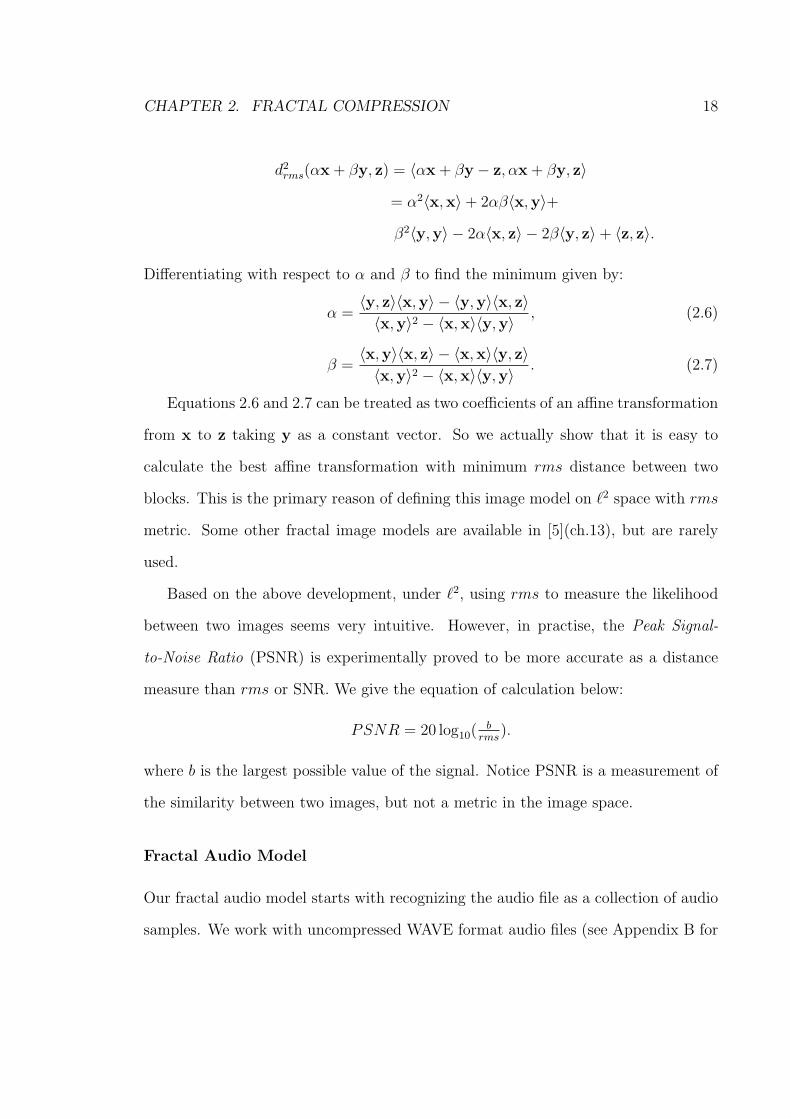
CHAPTER 2. FRACTAL COMPRESSION 18
d2rms(αx + βy, z) = 〈αx + βy− z, αx + βy, z〉
= α2〈x,x〉+ 2αβ〈x,y〉+β2〈y,y〉 − 2α〈x, z〉 − 2β〈y, z〉+ 〈z, z〉.
Differentiating with respect to α and β to find the minimum given by:
α =〈y, z〉〈x,y〉 − 〈y,y〉〈x, z〉〈x,y〉2 − 〈x,x〉〈y,y〉 , (2.6)
β =〈x,y〉〈x, z〉 − 〈x,x〉〈y, z〉〈x,y〉2 − 〈x,x〉〈y,y〉 . (2.7)
Equations 2.6 and 2.7 can be treated as two coefficients of an affine transformation
from x to z taking y as a constant vector. So we actually show that it is easy to
calculate the best affine transformation with minimum rms distance between two
blocks. This is the primary reason of defining this image model on `2 space with rms
metric. Some other fractal image models are available in [5](ch.13), but are rarely
used.
Based on the above development, under `2, using rms to measure the likelihood
between two images seems very intuitive. However, in practise, the Peak Signal-
to-Noise Ratio (PSNR) is experimentally proved to be more accurate as a distance
measure than rms or SNR. We give the equation of calculation below:
PSNR = 20 log10(b
rms).
where b is the largest possible value of the signal. Notice PSNR is a measurement of
the similarity between two images, but not a metric in the image space.
Fractal Audio Model
Our fractal audio model starts with recognizing the audio file as a collection of audio
samples. We work with uncompressed WAVE format audio files (see Appendix B for
CHAPTER 2. FRACTAL COMPRESSION 19
WAVE format). And further restrict the sample type to be unsigned such that each
sample can be treated as an integer from 0 to 255. Audio data is then a sequentially
stored vector of many samples with respect to time. The audio sequence is thus
treated in 1D space. It is easy to apply the above fractal image model in `2 with rms to
audio taking the advantage of the easy minimum distance calculation. Theoretically,
the two models are the same. Technically, the difference is the way of representing
the blocks. An image block is represented as a matrix of pixel values, and an audio
block is represented as a vector of sample values.
We have attempted to generate an audio sequence in 2D space, which puts the
samples into a matrix based on certain order like music sections, paragraphs, etc.
But unfortunately, we realize that a specific order can not be universally applied, and
there has not been any identified universal order or pattern that can be used. So, in
our implementation, we use 1D representation of audio as a sequential sample vector.
Psychoacoustics is a field that studies human perception of sounds. There is on-
going research to determine models of audio sequences that are perceived by humans
to be similar [8]. We take the straight rms distance as the measurement in our ex-
periments since no other proper measurement has been developed so far. Note that
it is possible to have two audio sequences with a high rms difference, but sound very
similar to our hearing, and vice versa. However, because our focus is on fractal coding
here, we think it is still appropriate to use rms as the measurement of the similar-
ity. Regarding more accurate audio measure, human acoustic testing may need to be
performed.
CHAPTER 2. FRACTAL COMPRESSION 20
2.3 Compression and Decompression Algorithm
We explain the compression and decompression algorithm based on our fractal audio
model. Compression is achieved from fractal encoding, and decompression is fractal
decoding.
2.3.1 Fractal Encoding
Our encoding is based on the PIFS. Our goal of encoding is to find a contractive map
set W whose fixed point is close to the audio space F 5 that we wish to compress. W
is the union of a set of contractive maps w1, . . . , wn from the PIFS.
Before we compute W , we have to partition our space F twice. Divide F into
disjoint range blocks R1, . . . , Rn, so that the union of Ri (i = 1, 2, . . . , n) covers F .
Divide F again into domain blocks D1, . . . , Dm. Then, for each Ri, we compare it
with all domain blocks to find Dj that can be mapped to Ri with the smallest rms
distance. Store Dj and wi from encoding as output. The following theorem ensures
W is contractive from the union of w1, . . . , wn.
Theorem 3. If w1, . . . , wn are contractive, then
W =⋃n
i=1 wi
is contractive in F with the sup metric.
Proof: Let s = maxi si, where si are the contractivities of wi.
5Space F with metric dsup (drms in this case) is complete.
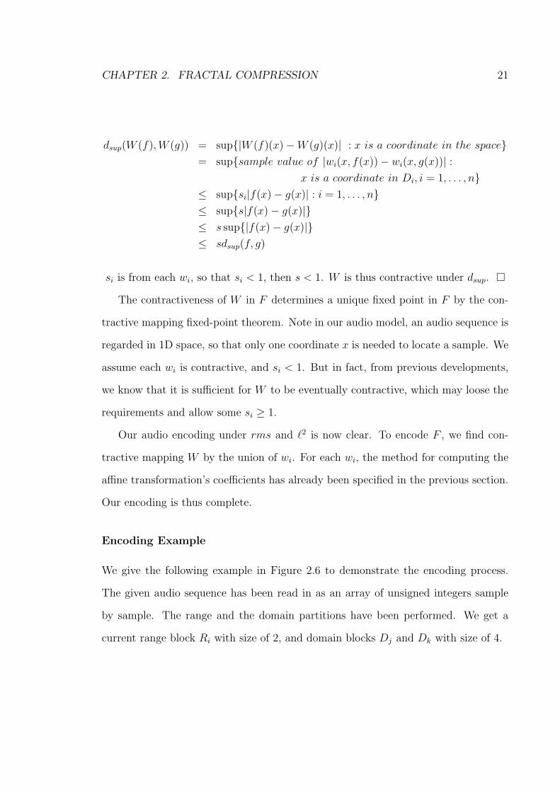
CHAPTER 2. FRACTAL COMPRESSION 21
dsup(W (f), W (g)) = sup{|W (f)(x)−W (g)(x)| : x is a coordinate in the space}= sup{sample value of |wi(x, f(x))− wi(x, g(x))| :
x is a coordinate in Di, i = 1, . . . , n}≤ sup{si|f(x)− g(x)| : i = 1, . . . , n}≤ sup{s|f(x)− g(x)|}≤ s sup{|f(x)− g(x)|}≤ sdsup(f, g)
si is from each wi, so that si < 1, then s < 1. W is thus contractive under dsup. ¤
The contractiveness of W in F determines a unique fixed point in F by the con-
tractive mapping fixed-point theorem. Note in our audio model, an audio sequence is
regarded in 1D space, so that only one coordinate x is needed to locate a sample. We
assume each wi is contractive, and si < 1. But in fact, from previous developments,
we know that it is sufficient for W to be eventually contractive, which may loose the
requirements and allow some si ≥ 1.
Our audio encoding under rms and `2 is now clear. To encode F , we find con-
tractive mapping W by the union of wi. For each wi, the method for computing the
affine transformation’s coefficients has already been specified in the previous section.
Our encoding is thus complete.
Encoding Example
We give the following example in Figure 2.6 to demonstrate the encoding process.
The given audio sequence has been read in as an array of unsigned integers sample
by sample. The range and the domain partitions have been performed. We get a
current range block Ri with size of 2, and domain blocks Dj and Dk with size of 4.
CHAPTER 2. FRACTAL COMPRESSION 22
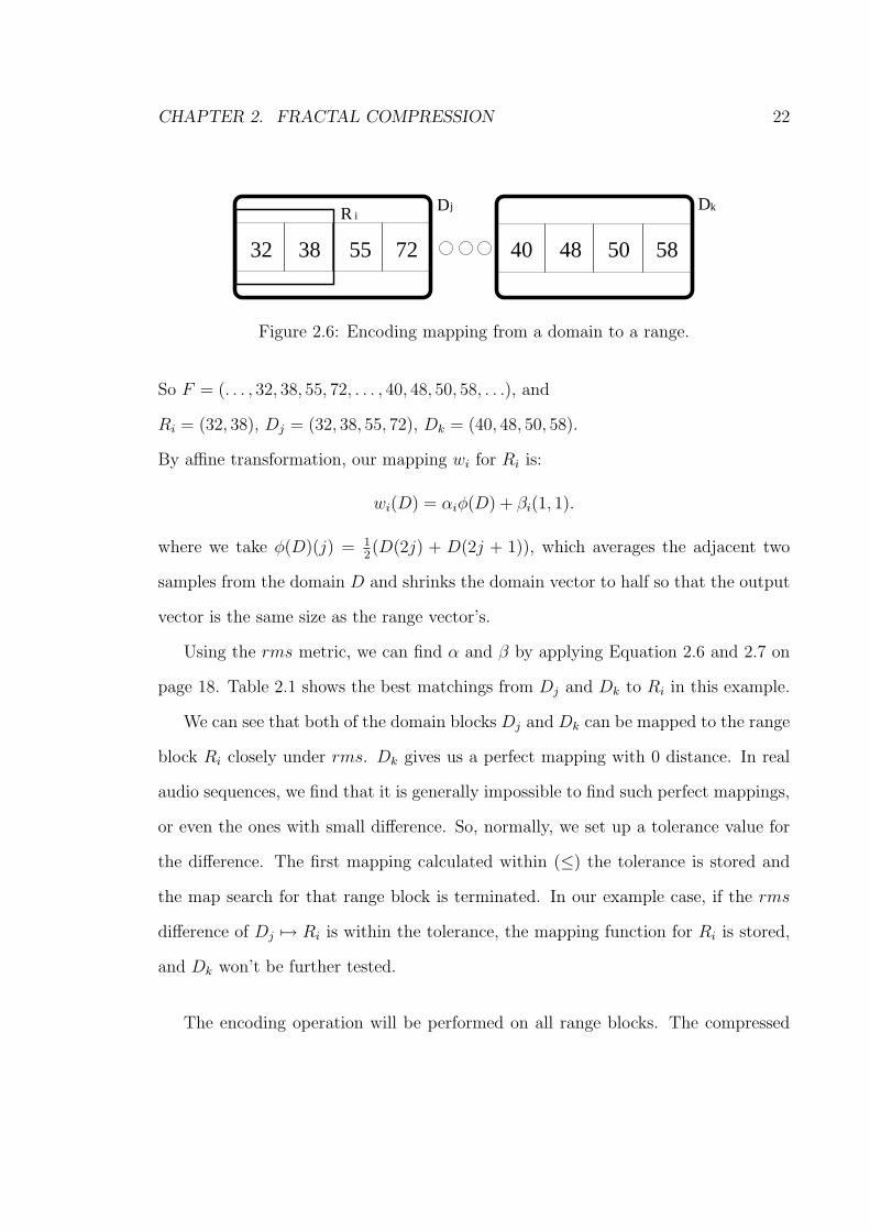
R D D
32 38 55 72 4840 50 58
kji
Figure 2.6: Encoding mapping from a domain to a range.
So F = (. . . , 32, 38, 55, 72, . . . , 40, 48, 50, 58, . . .), and
Ri = (32, 38), Dj = (32, 38, 55, 72), Dk = (40, 48, 50, 58).
By affine transformation, our mapping wi for Ri is:
wi(D) = αiφ(D) + βi(1, 1).
where we take φ(D)(j) = 12(D(2j) + D(2j + 1)), which averages the adjacent two
samples from the domain D and shrinks the domain vector to half so that the output
vector is the same size as the range vector’s.
Using the rms metric, we can find α and β by applying Equation 2.6 and 2.7 on
page 18. Table 2.1 shows the best matchings from Dj and Dk to Ri in this example.
We can see that both of the domain blocks Dj and Dk can be mapped to the range
block Ri closely under rms. Dk gives us a perfect mapping with 0 distance. In real
audio sequences, we find that it is generally impossible to find such perfect mappings,
or even the ones with small difference. So, normally, we set up a tolerance value for
the difference. The first mapping calculated within (≤) the tolerance is stored and
the map search for that range block is terminated. In our example case, if the rms
difference of Dj 7→ Ri is within the tolerance, the mapping function for Ri is stored,
and Dk won’t be further tested.
The encoding operation will be performed on all range blocks. The compressed
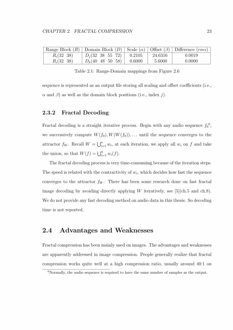
CHAPTER 2. FRACTAL COMPRESSION 23
Range Block (R) Domain Block (D) Scale (α) Offset (β) Difference (rms)Ri(32 38) Dj(32 38 55 72) 0.2105 24.6316 0.0019Ri(32 38) Dk(40 48 50 58) 0.6000 5.6000 0.0000
Table 2.1: Range-Domain mappings from Figure 2.6
sequence is represented as an output file storing all scaling and offset coefficients (i.e.,
α and β) as well as the domain block positions (i.e., index j).
2.3.2 Fractal Decoding
Fractal decoding is a straight iterative process. Begin with any audio sequence f06,
we successively compute W (f0),W (W (f0)), . . . until the sequence converges to the
attractor fW . Recall W =⋃n
i=1 wi, at each iteration, we apply all wi on f and take
the union, so that W (f) =⋃n
i=1 wi(f).
The fractal decoding process is very time-consuming because of the iteration steps.
The speed is related with the contractivity of wi, which decides how fast the sequence
converges to the attractor fW . There has been some research done on fast fractal
image decoding by avoiding directly applying W iteratively, see [5](ch.5 and ch.8).
We do not provide any fast decoding method on audio data in this thesis. So decoding
time is not reported.
2.4 Advantages and Weaknesses
Fractal compression has been mainly used on images. The advantages and weaknesses
are apparently addressed in image compression. People generally realize that fractal
compression works quite well at a high compression ratio, usually around 40:1 on
6Normally, the audio sequence is required to have the same number of samples as the output.
CHAPTER 2. FRACTAL COMPRESSION 24
images. Walle gives a very detailed analysis on fractal image encoding performance
compared with other conventional image compression methods in [24]. We do not
carry out experiments to compare fractal audio compression with other popular audio
compression methods such as MPEG and MP3 because audio coding is much more
complicated than image coding in general. The research here has been focused on
the behaviors of fractal coding on various types of audio data. Thus, we present the
advantages and weaknesses more from a general fractal model point of view.
Fractal Advantages
Fractal encoding is essentially a process to find close mappings, or transformations
if affine is required, for each range block from the domain blocks. We only need
to store the domain location and the coefficients of each transform after encoding.
Quite a lot of bits can then be saved over the original data. So the most valuable
advantage of fractal coding is the ability to achieve high compression ratios. However,
the compression ratio is highly dependent on identifiable patterns and self-similarities.
And thus, fractal coding with high compression ratio can not be universally applied.
In audio compression, we can see that fractal audio coding is a much simpler
scheme at this stage compared with the most popular MP3 encoding. The simplicity
may be considered as one potential advantage that fractal coding can be used in the
audio world. And despite the fact that audio is a very continuous sequence, it still
embeds patterns and self-similarities, especially those created by us, like music and
instrumental sounds, which gives us a hope of applying fractal coding.
CHAPTER 2. FRACTAL COMPRESSION 25
Fractal Weaknesses
Fractal compression has not been put into practical use for its numerous weaknesses.
The success of the scheme seems to rely exclusively on exhibiting some self-similarities
among part of the space. And there is no guarantee that the probability of matching
domain and range blocks is sufficiently high to achieve good compression.
Our restriction of using affine mappings does not guarantee scaling αi and offset
βi forming a set of independent random variables. This is to say that each wi may
not be able to independent from others. In other words, different orders of applying
wi may result different decoding sequences.
Furthermore, fractal encoding uses a large amount of time because of the extensive
search for matching blocks, and fractal decoding can also be a time-consuming process
as addressed in the previous section.
2.5 Conclusion
Throughout this chapter, we have given the theoretical background on how fractal
compression works. We prove the possibility of applying fractal coding by defining
the complete metric space on image and audio. Some details of the fractal encoding
and decoding based on `2 space and rms metric are also discussed. Partition and
mapping of the domain and range blocks have been particularly addressed.
The theory behind fractal compression and the motivation of applying fractal
coding to audio data have been presented. However, the theoretical performance of
fractal audio coding is still far from clear. We thus consider experiments, which may
help us to gain more knowledge.
Chapter 3
A Review of Relevant Literature
3.1 Introduction
This chapter is a review of the main literature on the subject of fractals. We take
a look at fractal coding from its various perspectives. Some related questions are
addressed. We do not give concrete treatments on most of the aspects, which would
be out of the scope here. A basic knowledge of fractal coding is assumed.
The fundamental principle of fractal coding consists of the representation of a
space by a contractive transform of which the fixed point is close to the space. Most
current fractal studies focus on images, because 2D image space is naturally repre-
sented as a complete metric space via the norm distance measure. However, fractal
encoding is not as simple with no known algorithm for constructing the transform
with the smallest possible distance between the corresponding fixed point and the
image to be encoded. A common suboptimal approach taken by most researchers
in this area is to construct the transform as a “collage” or union of mappings from
the image to itself, and a sufficiently small “collage error” (the distance between the
26
CHAPTER 3. A REVIEW OF RELEVANT LITERATURE 27
collage and the image) guarantees that the fixed point of that transform is sufficient
close to the original image.
Taking the collage approach leads us to the problem of identifying the mappings
quickly. This problem was settled by applying Partitioned Iterated Function Systems
(PIFS) [9]. The idea is to localize the search to small subsets of the whole space.
However, the fractal scheme based on the collage and PIFS clearly leaves considerable
latitude in the design of a particular implementation. Wohlberf and Jager classified
the majority of existing fractal image coding schemes into five categories [26]:
• The partition imposed on the image determined by the range blocks.
• The composition of the pool of domain blocks.
• The class of transforms applied to the domain blocks.
• The type of search used in locating suitable domain blocks.
• The representation and quantization of the transform parameters.
There are few theoretical results on which design decisions in any of these aspects
may be based. So fractal image coding has remained in the research area until now.
There have been few attempts to extend fractal coding to other types of data. Fractal
coding on video has been investigated in [3] and [29]. Fractal audio coding has been
discussed in [24], which is the focus of this thesis.
3.2 Fractal Coding Problems
Fractal coding is essentially a way of identifying self-similarities or patterns in a
space through transforms and hopefully to achieve compression by only storing the
CHAPTER 3. A REVIEW OF RELEVANT LITERATURE 28
transform coefficients. However, to find such self-similarities is not a trivial problem
as we have described above. Even with the collage and the PIFS, there are still
many choices when designing a fractal coding scheme for a type of data. We review
some common problems addressed within the large amount of fractal literature below.
Most of them are in fractal image coding, since image compression is the subject where
fractal coding was introduced and mainly studied.
3.2.1 Partition Scheme
Based on the PIFS, we have to partition our space into subspaces. The range and the
domain partitions determine the process of finding the mappings from the domain
blocks to the range blocks. The partition schemes are most critical for the range
partition. The domain partition is based on the range partition since the domain
shape and size are restricted by the range’s, because we use an affine transformation
from domain to range. A wide variety of partition schemes have been investigated,
with the majority being composed of rectangular blocks. We only discuss some pop-
ular schemes here, and for the reader interested in this aspect, refer to [26] for more
detailed treatment.
Quadtree
Quadtree partitions were used in the first implementation of the PIFS based fractal
image coding [9]. It employs the well-known image processing technique based on
a top-down recursive splitting of selected image quadrants. The resulting partition
can be represented by a tree structure in which each non-terminal node has four
descendants. This partition scheme is easy to implement because of its recursive
CHAPTER 3. A REVIEW OF RELEVANT LITERATURE 29
structure, which allows us to automatically discard the larger block prior to splitting
it into four subblocks if an error threshold was exceeded. Various sized range blocks
can be set up by restricting the recursive depth. We can also first partition the space
into uniform sized “smallest” blocks. We then proceed using the bottom-up approach
to merge those neighboring blocks to get a larger block one level up the quadtree if the
error is below the threshold. The first top-down approach has been discussed in [2],
[5] (ch.3), and [11] (pg.93-105), and the latter bottom-up approach was introduced
in [11] (pg.93-105).
Horizontal-Vertical
The Horizontal-Vertical (HV) partition scheme can be recognized as a generalized
quadtree scheme with the splitting done by a horizontal or vertical line. It was
discussed in [5] (ch.6). The HV scheme gives more freedom for finding similarities,
but more work on defining the domain blocks since the range blocks from the HV
partition are more variable in size and shape. Nevertheless, HV partitions still gives
a tree structure result and the partitioned blocks are still rectangular.
Non-Rectangular
There are some partition schemes not based on rectangular blocks. In the article by
Wohlberg and Jager [26], they give the basic idea of how it works. The motivation
behind the non-rectangular partition scheme is to better preserve self-similarities in
subspaces after the partition. And in most cases, it is obvious that using only rectan-
gular partitions can not give us the optimal result in terms of maximally preserving
self-similarities.
CHAPTER 3. A REVIEW OF RELEVANT LITERATURE 30
Overlapped Range Blocks
Some out-of-box partition schemes allow overlapping among the range blocks, which
is different than the original idea of the PIFS from Jacquin [9]. Reusens used an
overlapped quadtree scheme with multiple domain transforms [20] to reduce block
artifacts. Walle also claimed to further overcome the block artifact by allowing the
range blocks to overlap [24]. Those techniques, while promising some improvements,
do increase the complexity of the encoding process.
Comparison
Most of the fractal coding implementations use the quadtree partition scheme. Very
few researchers have reported comparisons by applying different schemes. Review [26]
gives some comments from different papers. But unfortunately, the results do not
agree with each other. We have not found any implementation based on a non-
rectangular partition scheme. A difficulty in partitioning with more complicated
shapes, is that determining a distance measure becomes exceedingly complicated.
Partition schemes of fractal coding on other types of data is basically untouched
because fractal coding theory has not been proven efficient on any new type of data
except for images. However, it is expected that the partition scheme may be very
different when dealing with different types of data.
3.2.2 Domain Pool
The domain pool used in fractal compression is often referred to as a “virtual code-
book”. The domain pool is a collection of the domain blocks, which are used to
CHAPTER 3. A REVIEW OF RELEVANT LITERATURE 31
compare the range blocks to find mappings. So the size of the domain pool, deter-
mined by how many domain blocks are in the pool, is crucial to the efficiency of the
encoding. The general sense is that the larger the domain pool is, the better fidelity
(i.e., smaller distance) of the mappings between the domain blocks and the range
blocks. On the other hand, larger pools lead to more comparisons, which slows down
the encoding. Some research has been done to reduce the size of the domain pool
by applying some restrictions when choosing the blocks while not sacrificing mapping
fidelity too much.
Global Domain Pool
The naıve domain pool design is to have a fixed domain pool for all range blocks.
This design is identified by empirical evidence on image compression where the best
domain block for a particular range block is not expected to be spatially close to
that range block to any significant degree [5] (pg.69-71) [26]. However, this simple
approach results in a domain pool with an enormous size. Further restrictions have
to be applied to reduce the size of the pool to bring the encoding process into a
manageable time frame.
The common approach started by Jacquin [9] is to restrict the domain block to
twice the length 1 of the range block. This is supported by the argument that the
larger sized domain block of the two corresponding domain pools usually gives a
better compression ratio and fidelity of recovery [30]. Under this restriction, one
domain pool only applies to certain sized range blocks. General larger sized domain
pools which contain the domain blocks larger than the given range block cannot be
1Note that the length is measured by dimensions. So for a 2D image range block, the domainblock is twice the length on both the width and the height.
CHAPTER 3. A REVIEW OF RELEVANT LITERATURE 32
applied here because the distance metric would be very difficult to define.
In most of the designs, the size of the range block is further restricted to guarantee
compression. Many fractal image compression schemes require the range block to be
no smaller than 4 pixels by 4 pixels, which also implies a size restriction on the domain
block from previous descriptions. The restrictions on both the range and the domain
are considered when taking fractal coding to other types of data [25] [29].
Classification Domain Pool
The domain blocks in the domain pool are usually classified before the map search.
In the encoding process, one range block can be compared to only one class of the
domain blocks from the pool that belongs to the same category to reduce the total
amount of comparisons. The domain and range blocks are commonly classified into
a fixed number of classes according to a certain classification scheme [5] (ch.3, 4) [9].
Other ways of doing classification without a restriction on the number of classes are
possible [26], however, difficult to grasp.
There are a variety of classification schemes. It is not hard to see that different
schemes are needed for different types of data. We regard classification as a potential
way of getting an efficient fractal domain pool on audio data in our research.
Local Domain Pool
In the article by Wohlberg and Jager [26], they describe the effort of localizing the
domain pool for each range block to a region about the range block, or a spiral search
path that may be followed outwards from the range block position. The idea comes
from the experimental tendency for a range block to be spatially close to the matching
CHAPTER 3. A REVIEW OF RELEVANT LITERATURE 33
domain block on images. The localized domain pool thus gives a smaller search space
for each range block. Some evidence from [11] (pg.122) shows that the local pools
outperform the global ones. Some other ways of forming local domain pools are also
discussed in [26].
However, it is not yet clear how the local domain pool can be applied to fractal
coding on other types of data. No experiments have been done to show such a
tendency on other types of data except for images. Different ways of forming local
domain pools may need to be developed to improve encoding efficiency.
Hybrid Codebooks
It is agreed that Vector Quantization (VQ) may perform slightly better than fractal
coding in some cases of image compression with more predictable outcomes. A hybrid
domain pool design with VQ was discussed in [17], which also improves coding speed.
The idea of applying adaptive techniques to fractal domain pool design was
pointed out in [5] (ch.9), and [25]. The fractal domain pool design with adaptive
technique seems attractive to us in applying fractal coding on audio data, because
audio is usually represented as a sequential stream.
Discussion
Most of the techniques of designing an efficient domain pool we have discussed here
are essentially attempts to localize the domain pool for the range blocks; in other
words, to reduce the size of the domain pool to cut the number of comparisons for
searching the mappings. Classification is probably a more promising technique than
others, while the process is highly dependent on the classification scheme. Hybrid
CHAPTER 3. A REVIEW OF RELEVANT LITERATURE 34
codebook design is complicated, and hard to be implemented in general.
The differences of the domain pool design are significant and depend on different
types of data in most cases, which make the comparison of those techniques difficult.
3.2.3 Decoding
The decoding process of fractal coding is a reconstruction through iteratively applying
the mappings (transforms) from the encoding in reverse. Theoretically, by the fixed
point theorem, starting from an arbitrary sequence, the reconstruction leads to a fixed
sequence. And the collage and complete metric space requirements provide that the
final fixed sequence shall be close to the original sequence with a sufficiently small
error.
Standard Decoding
Standard decoding is a straightforward process. In most cases, we start from an initial
zero vector, and specify the number of iterations. Then apply reversed mappings
iteratively. Experiments in [2], [9], and [30] on fractal image decoding have shown
that fractal decoded images generally converge to a fixed image after 10 iterations.
The standard decoding suffers a big problem of slow speed. One way to improve
the decoding speed is to find mappings that converge faster in the encoding stage,
so that fewer iterations are needed in the decoding process. Some studies have been
done [5] (C.13) relating the problem with the threshold of the allowable distance
between the domain block and the range block when identifying the mappings.
CHAPTER 3. A REVIEW OF RELEVANT LITERATURE 35
Fast decoding
There are other methods to decode. It is possible to find the exact fixed point directly
by inverting a large but sparse matrix [5] (ch.11). Then the further development of the
fractal hierarchical model [5] (ch.5) gives a fast decoding algorithm by approximating
the fixed point in a lower-dimensional space, where the range block dimensions are
doubled at each step, until the desired size is reached. A considerable computational
saving is obtained by applying the standard iterative method to full-sized blocks [26].
Postprocessing
Postprocessing is mainly addressed with the problem of blocking artifacts in the de-
coded image [5] (pg.59) [11] (pg.222-224). Based on PIFS, our range partition results
in blocks that are disjoint, which may introduce blocking artifacts after decoding.
This problem has not been considered to be serious in fractal coding theory, because
allowing the domain blocks to overlap already reduces strong blocking artifacts. The
idea of further allowing the range blocks to have certain degree of overlap, which
may give a even smoother edge between blocks, has been reviewed in the previous
section. However, postprocessing may be very useful when applying fractal coding
on other types of data. The processing methods can be more advanced with some
sophisticated transform techniques.
Multiple Resolution
One advantage of fractal coding being cited is resolution independence [5] (pg.59) [26].
The fractal model uses functions of infinite resolution. Therefore, we may pick any
resolution from the decoding. Taking images for example, we may decode an encoded
CHAPTER 3. A REVIEW OF RELEVANT LITERATURE 36
image to a larger sized one that still encodes the original information. However,
studies [5] (ch.5) have shown that the enlarged image contains artificial data created
by the transformations. The resolution independence feature does not show any
interest to us for applying fractal coding to other types of data.
Multiple resolution has also been recognized in another way related to wavelet
transforms [22] [24] [26]. The wavelet representation of fractal coding gives the po-
tential of joining the two to improve the reconstruction fidelity while maintaining
high compression ratio from fractal coding. This theory may also be more generally
applied to other types of data.
3.2.4 Efficient Storage
In order to achieve a better compression ratio, the bit allocation schemes for storing
the transform coefficients and the partition parameters are important. The simplest
scheme is to quantize them uniformly [5] (ch.3). The bit allocation scheme of 5 bits
for the scaling coefficient, and 7 bits for the offset coefficient was reported to provide
the best performance on fractal image coding [5] (pg.61-65). The partition parameter
is based on the partition scheme. In the top-down quadtree partition scheme, only
one bit is needed to indicate whether to continue at each recursive partition step for
a range block. The domain blocks are usually indexed and referenced by the indices.
We can further save bits when the scaling value is zero, and the domain is irrelevant
to the transformation and need not be stored.
Some investigation has been done to optimize the bit allocation through non-
uniform quantization [26]. However, no significant improvement over uniform quan-
tization was found.
CHAPTER 3. A REVIEW OF RELEVANT LITERATURE 37
In other work, statistical analysis was used to correlate scaling and offset co-
efficients between neighboring blocks [10]. This correlation is then used to obtain
improved quantization [11] (pg.140-144).
The bit allocation optimizing methods for fractal coding have not been widely im-
plemented because of the complexity added to both encoding and decoding processes.
The difficulty of applying some optimizing method suggests that it may be better to
stay with the simple uniform quantization with an experimentally optimized setting.
3.3 Hybrid Fractal Coding
In data compression, many conventional methods have been established on different
types of data, and often hybrid methods are also investigated by joining two or more
compression methods. Walle [24] reviewed fractal coding with some conventional
transform methods such as Discrete Cosine transform (DCT) or wavelet transforms,
and demonstrated the relationship between the two. This relationship fits well with
fractal coding because it too uses transformations. The conventional transform meth-
ods were also introduced to image compression in the first place with a solid statistical
foundation. Researchers have found that the transform methods work better at low
compression ratios while fractal coding works better at high compression ratios in
general.
Different transform methods have been applied with fractal coding to form some
hybrid fractal coding schemes. With some transform methods being more widely used
on other types of data to achieve good compression, hybrid fractal coding has gained
significant interest recently. We address two popular hybrid fractal coding methods
that are still under research in this section. The DCT is described in [16] or any data
CHAPTER 3. A REVIEW OF RELEVANT LITERATURE 38
compression book; for the wavelet treatment related to fractal coding, see [7] [22] [23].
3.3.1 DCT and Fractal Coding
The DCT is a widely used transform technique in image compression, which is part
of the JPEG standard. The DCT has been recognized with the ability of removing
inter-pixel redundancies with an efficient implementation. Hybrid DCT fractal coding
generally tries to combine the advantage of the DCT with the ability of capitalizing
on long-range correlations within the image from fractal coding [15]. Fisher, Rogovin,
and Shen compared fractal coding with the DCT based JPEG coding [28], and showed
their different advantages. Melnikov and Katsaggelos recent developed a jointly op-
timal fractal/DCT compression scheme [15]. Their hybrid scheme takes the DCT on
selected blocks. It then uses fractal coding on the quantized DCT coefficients. The
operational optimality comes from applying the Lagrangian multiplier approach on
the hybrid transform parameters [15].
The complementing nature of fractal and DCT suggests their joint use to maxi-
mally remove the redundancies in an image. However, the DCT has its weaknesses.
The most cited one is the block artifact [9]. The hybrid scheme from [15] basically
allows the range block to be joined to resolve this problem. The question of whether
self-similarities among an image are preserved after the DCT has not been addressed.
Furthermore, not enough experiments have been done to fully understand the perfor-
mance of the hybrid scheme.
We also realize that fractal/DCT hybrid scheme has limited potential since the
DCT is primarily developed on the image compression field only [24] [28]. So, gener-
ally speaking, the DCT is not very helpful for applying fractal coding on other types
CHAPTER 3. A REVIEW OF RELEVANT LITERATURE 39
of data.
3.3.2 Wavelet and Fractal Coding
Wavelet analysis was developed in the late 1980s [13] [14], and extensively explained
in [18] and [19]. A significant development in fractal coding theory is recognizing
fractal coding through wavelet analysis as discovered by a number of researchers
independently [7] [22] [23]. Hybrid wavelet and fractal coding schemes use the iterated
function system to generate wavelet coefficients from the wavelet transform.
This discovery also gives a better understanding of the mechanism underlying
standard fractal coding. If the domain increment is equal to the domain block size,
and subject to a few additional restrictions [5] (pg.95), there is a direct correspondence
between the domain and range blocks in fractal coding. Under this case, the domain
and range mapping is equivalent as the mapping between the subtrees rooted at
consecutive resolutions in the Haar wavelet transform [26]. This relationship demon-
strates the natural expression of fractal coding from the wavelet transform point of
view. And the PIFS based fractal image coding scheme is comparable to a Haar
wavelet subtree quantization scheme [4].
A number of hybrid coders have been implemented, combining the subtree map-
ping of fractal coding with some scalar quantization techniques of various complex-
ities [4] [12] [23] [24]. The high frequency wavelet coefficients are encoded using a
collage approach from fractal coding. Walle [23] further allowed the wavelet trans-
form coefficients to be directly stored if no mapping could be identified within certain
error threshold in the hybrid image compression scheme. Their study showed that
at a low compression ratio (i.e., high picture quality), few mappings can be found

CHAPTER 3. A REVIEW OF RELEVANT LITERATURE 40
and most wavelet coefficients have to be stored. Fractal compression only starts to
play a significant role at high compression ratios. Experimental results [4] [23] also
suggest that applying a smoother wavelet with additional vanishing moments leads
to a better compression of the signal.
One main advantage of this hybrid scheme is significantly reducing the block
artifacts [23]. Through the ability of generating multi-resolutions, artifacts can be
overcome by combining different resolutions from the wavelet transform. The rms
norm is preserved under the orthogonal wavelet transform, which means minimizing
the rms metric between the wavelet transform coefficients is equivalent to minimizing
the rms metric between the actual signal blocks. The wavelet framework can also be
applied to develop an unconditionally convergent hybrid scheme [4], which admits a
fast decoding algorithm.
Patel, Tonkelowitz, and Vernal directly applied the wavelet transform to audio
compression to form a lossless scheme [1]. Their experiments suggested that the
wavelet transform alone might not be the right paradigm for lossless sound compres-
sion. Wannamaker and Vrscay applied their fractal wavelet hybrid scheme on audio
data [25], and showed that the compression ratios above 6:1 might ultimately be at-
tainable with a good fidelity signal reconstruction. Applying the wavelet transform
on audio data also has the potential advantage to overcome fractal coding’s inability
to simulate continuous wave signals, which may be a way of helping fractal coding on
audio data.
CHAPTER 3. A REVIEW OF RELEVANT LITERATURE 41
3.4 Conclusion
We have given a short review of the current state of fractal coding. The use of fractal
coding is primarily on image data. Unfortunately, to date, we know of no widespread
use of fractal image coding.
Compressing audio data with fractal coding is a natural next step, however, there
has been very little work done in this area. Therefore, preliminary and exploratory
examination of fractal audio coding is required.
It should be noted that the majority of fractal coding algorithms that have been
recently developed are not classical fractal coding algorithms relying purely on finding
the self-similarity, but incorporate other techniques to identify redundancy. It is still
not clear whether fractal coding can capture statistical properties effectively, and
compete with other types of compression methods. The potential of fractal coding
on image and audio data remains to be seen.
Chapter 4
Implementation and Empirical
Results
This chapter describes the implementations of a binary partition fractal coding scheme
for audio data. This fractal audio scheme is comparable with the conventional fractal
image scheme based on the quadtree partition that has appeared in many previous
papers on fractals.
The empirical results from applying the scheme to our test audio data are pre-
sented. Various tests concentrating on different aspects of fractal audio coding are
performed. We make some conclusions and suggestions from our empirical studies on
fractal audio coding at the end.
It is noticeable that our fractal coding scheme is heuristic based. We make no
comparison to the state-of-art audio compression methods. Our focus here is to
explore the possibility of applying fractal coding on different audio data.
42
CHAPTER 4. IMPLEMENTATION AND EMPIRICAL RESULTS 43
4.1 Fractal Audio with Binary Partition
4.1.1 Encoding
The encoding process follows Fisher’s conventional fractal encoding algorithm [5]
(pg.19). Binary partition has been used based on the representation of audio data
as a sample sequence in 1D space. Simple classification has been applied to improve
encoding efficiency.
The Ranges and Domains
The range and domain blocks in fractal audio coding are based on audio samples.
The size of the block is the number of audio samples in the block. We restrict the
domain block size to be twice of the range block’s, and each range block to contain at
least four samples. The range blocks are selected based on the binary partition and
the affine mapping. The initial partition is to partition an audio sequence into four
subsequences. Then the four resulting range blocks are compared with all potential
domain blocks from the domain pool to find the optimal domain blocks achieving
the minimum rms distance through affine transforms. If the minimum rms distance
is above the permitted error threshold, we recursively divide the range block into
two subblocks applying the binary partition. This process is repeated until a range
block can be mapped to a potential domain block with a minimum rms distance
less than the error threshold, or the smallest range block size has been reached. In
the latter situation, we store the transform with the minimum rms distance at the
deepest recursive level (i.e., with the smallest range block size). Once a mapping wi
has been identified, we store the transform coefficients (i.e., scaling and offset) and
CHAPTER 4. IMPLEMENTATION AND EMPIRICAL RESULTS 44
the range block and domain block locations to the output file. The range block which
has been mapped is discarded after. The final output file stores parameters of the
map W =⋃
wi from the encoding process.
We allow three kinds of domain pools (D1,D2,D3). D1 has a lattice with a fixed
spacing l, which means the domain blocks from D1 are directly obtained from a fixed
size window sliding l samples each time through the whole sequence. Setting l to 1
gives us all possible domain blocks for a range, which is the default in our experiment.
D2 is formed with a spacing given by the domain size divide by l, which gives more
small domain blocks and less large ones. The D2 domain pool thus concentrates on
the small size range blocks to ensure mapping quality. D3 has a lattice as D2 does but
with the opposite spacing-size relationship, which means the largest domain blocks
have a spacing corresponding to the smallest domain size divided by l, and vice versa.
The D3 domain pool thus has more large domain blocks, and less small ones. The
idea is that it is more important to find a good domain-range fit for larger range
blocks, because the encoding will require a fewer number of transforms [5] (pg.57),
which also means a higher compression ratio.
Based on the general restrictions on the range size, the range blocks can be sized
from the second recursive partition to the minimum size (i.e., 4 samples). For example,
an audio sequence that contains 2n samples can have a maximum range block size
of 2n−2, and minimum size of 4. The theoretical largest size range block (i.e., size of
2n−1) is almost impossible to be mapped by the whole sequence with a sufficiently
small error, and a range size less than 4 may cause compression failure because too
many mappings may occur at the small size range blocks. For the above reasons, we
consider the size restriction in our implementation necessary.
CHAPTER 4. IMPLEMENTATION AND EMPIRICAL RESULTS 45
The Classification
The domain-range comparison step of fractal encoding is very computationally in-
tensive. Different classification schemes have been invented to minimize the number
of domain-range comparisons starting from Jacquin’s original work on fractal image
compression [9]. The basic idea is to categorize the domain blocks under certain cri-
teria before the encoding actually takes place. During the encoding, one range block
is classified using the same scheme, and only needs to be compared with the domain
blocks in the same category. By reducing the number of domain-range comparisons,
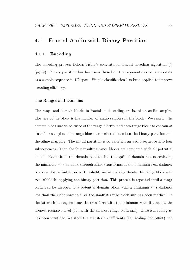
the classification improves fractal encoding efficiency. Jacquin classified an image
block into flat, edge, and texture regions. Many later classification approaches can
be referred to, see [11] and [28].
Our classification scheme for audio fractal encoding is very intuitive, and can be
treated as a simplified version of the one presented in [28]. Fisher used a scheme
that divided an image block into upper left, upper right, lower left, and lower right
quadrants, which are numbered sequentially. For each quadrant, the sum and the
variance of the pixel values are computed. So, if the pixel values in quadrant i are r1,
r2, ..., rn, for i = 1, 2, 3, 4, they compute:
Sum: Ai =n∑
j=1
rij Variance: Vi =
n∑j=1
(rij)
2 − A2i .
It is shown that it was always possible to orient one block into one of three canonical
positions with the brightest (i.e., largest pixel sum) block located at upper left as
shown in Figure 4.1. The classification scheme has 3 major classes based on canonical
positions, and 24 subclasses consisting of the 24 orderings of the Vi for each major
CHAPTER 4. IMPLEMENTATION AND EMPIRICAL RESULTS 46
class. The transformation of orienting one domain into one canonical position is
recorded during the classification process.
(a) Major Class 1:A1 ≥ A2 ≥ A3 ≥A4
(b) Major Class 2:A1 ≥ A2 ≥ A4 ≥A3
(c) Major Class 3:A1 ≥ A4 ≥ A2 ≥A3
Figure 4.1: Four quadrants of an image block can always be oriented so that the sumvalues of the quadrants fall into one of these three canonical positions.
The above classification scheme works well on fractal image encoding with quadtree
partition. It is very general as not based on any specific image block attribute. We
adopted this scheme into fractal audio coding. However, audio sequence is treated
as 1-dimensional data in our case. Binary partition is used for this encoding. We
thus simplify the classification scheme to divide an audio block into left half and right
half. Organize each block, either range or domain, into the canonical position with
the bigger sum of the sample values 1 half left. So, one block is either rotated or
not in our scheme. We have 2 classes from the classification by the orderings of the
variance Vi, either V1 ≤ V2, or V1 > V2 as Figure 4.2 on the next page shows.
1Each sample is recognized as an unsigned integer in our case, see Appendix B for detail.
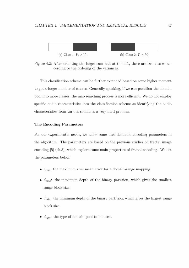
CHAPTER 4. IMPLEMENTATION AND EMPIRICAL RESULTS 47
(a) Class 1: V1 > V2 (b) Class 2: V1 ≤ V2
Figure 4.2: After orienting the larger sum half at the left, there are two classes ac-cording to the ordering of the variances.
This classification scheme can be further extended based on some higher moment
to get a larger number of classes. Generally speaking, if we can partition the domain
pool into more classes, the map searching process is more efficient. We do not employ
specific audio characteristics into the classification scheme as identifying the audio
characteristics from various sounds is a very hard problem.
The Encoding Parameters
For our experimental needs, we allow some user definable encoding parameters in
the algorithm. The parameters are based on the previous studies on fractal image
encoding [5] (ch.3), which explore some main properties of fractal encoding. We list
the parameters below:
• erms: the maximum rms mean error for a domain-range mapping.
• dmax: the maximum depth of the binary partition, which gives the smallest
range block size.
• dmin: the minimum depth of the binary partition, which gives the largest range
block size.
• dtype: the type of domain pool to be used.
CHAPTER 4. IMPLEMENTATION AND EMPIRICAL RESULTS 48
• l: the lattice spacing used in the domain pool.
• smax: the maximum allowable scaling factor of an affine transform.
In our algorithm, dmax is n − 2 and dmin is 2, where n is the power of 2 of the
audio sequence size in samples. dtype can be set to 1, 2, or 3 to use domain pool D1,
D2, or D3. smax is usually 1 to guarantee absolute contractiveness2.
We have some of other encoding parameters not related with the algorithm. The
parameters si and oi specify the numbers of bits to store scaling and offset coefficients
of a transform. The full search flag can be set to true to bypass the classification
scheme allowing all possible domain blocks to be compared with a range block. The
audio header parameter specifies the length of the audio format information (see
Appendix B for details). Different versions of the WAVE format may be applied
with different header lengths. We allow the maximum audio sequence to contain 220
samples in our experiments. Audio sequences which contains more than 220 samples
will be divided into frames with a length of 220 samples each, then encoded frame by
frame as in [25].
4.1.2 Decoding
We take the natural fractal decoding process by iterating map W from the encoding
in reverse. Fast decoding methods, as mentioned in Section 3.2.3 can not be applied
here since the underlying model is based on images. The coefficients of the transforms
are read in from the encoded file. A map wi can be reconstructed based on the affine
transform definition that R = αD + β, where R is a range block, and D is a domain
block. W then can be reconstructed by the union of wi. The decoding algorithm here
2see Section 2.2.2 for details.
CHAPTER 4. IMPLEMENTATION AND EMPIRICAL RESULTS 49
is not efficient and likely to be time-consuming. However, decoding efficiency is not
our interest here.
The Iteration
We start decoding from a zero sequence that has the same number of samples as the
original audio sequence. At each iteration, we apply the map W in reverse to the
sequence, and replace the sequence with the new one.
Base on the previous studies on fractal image decoding, we use 10 iterations by
default. We calculate the difference between consecutive iterations to compare the
contractivity. It is also possible to set up a threshold, which can be used to compare
the difference between two consecutive iterations. And if the difference is below the
threshold value, the decoding process can be halted. However, at this point, we are
not sure about which value of the threshold is appropriate. Fractal theory seems to
give no support on this issue either.
The Decoding Parameters
Most decoding parameters are straight forward coming from the encoding in order to
get the best approximation of the original audio sequence.
• ni: the number of iterations in the decoding process.
• dmax: the maximum depth of the binary partition, which gives the smallest
range block size.
• dmin: the minimum depth of the binary partition, which gives the largest range
block size.
CHAPTER 4. IMPLEMENTATION AND EMPIRICAL RESULTS 50
• dtype: the type of domain pool to be used.
• l: the lattice spacing used in the domain pool.
• smax: the maximum allowable scaling factor of an affine transform.
dmax, dmin, dtype, and l are read in from the encoded file. smax and other parameters
si and oi have to be consistent with the encoding. The different setup may cause a
bad decoding sequence. The postprocessing flag allows the averaging process between
the decoded blocks to take effect after each iteration or after number of iterations.
This is somehow a very general approach to see whether smoothing block edges may
give us better recovery of an audio sequence from the encoded file.
4.2 Testing Setups
4.2.1 Testing Audio Data
In order to test our compression scheme and parameter settings, we use five groups
of audio data in WAVE format from different references. The WAVE files are listed
in the table of Appendix A on page 74.
The five categories are intuitive representations of different audio data. Note
that we do not formally classify audio data here, but use some common sense. The
speech category contains the WAVE files recording different people talking. The
instrumental category has the WAVE files with instrumental sounds. The singing
songs with background music are in the music song category. The sound clips are
various short sounds from different actions. Finally, we make some special WAVE
files for our testing purposes in the others category.
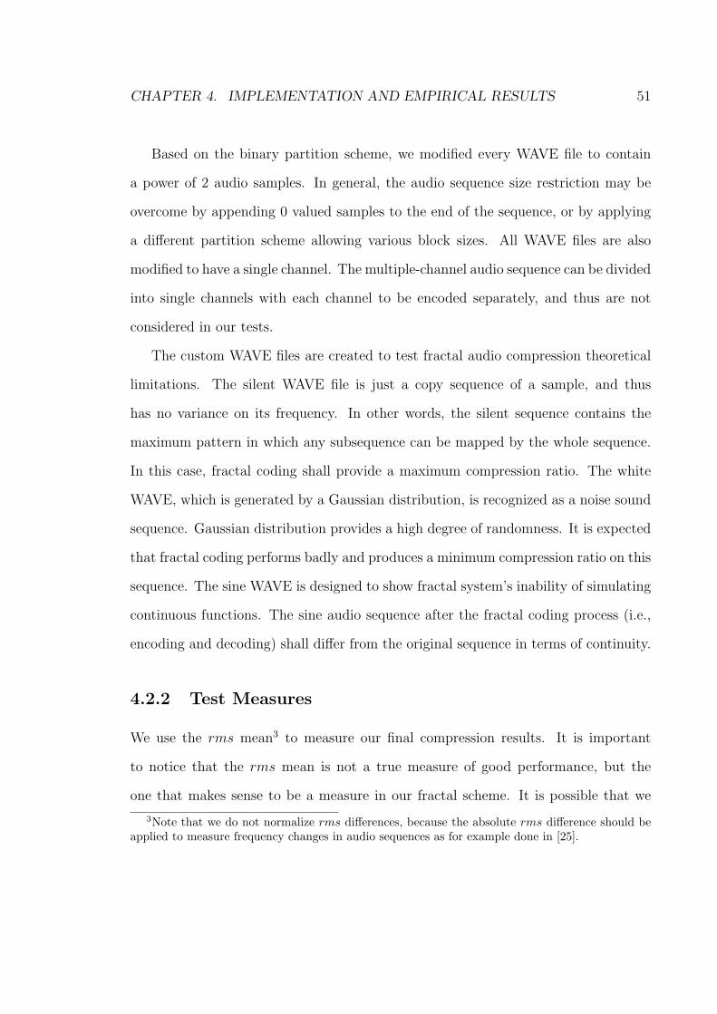
CHAPTER 4. IMPLEMENTATION AND EMPIRICAL RESULTS 51
Based on the binary partition scheme, we modified every WAVE file to contain
a power of 2 audio samples. In general, the audio sequence size restriction may be
overcome by appending 0 valued samples to the end of the sequence, or by applying
a different partition scheme allowing various block sizes. All WAVE files are also
modified to have a single channel. The multiple-channel audio sequence can be divided
into single channels with each channel to be encoded separately, and thus are not
considered in our tests.
The custom WAVE files are created to test fractal audio compression theoretical
limitations. The silent WAVE file is just a copy sequence of a sample, and thus
has no variance on its frequency. In other words, the silent sequence contains the
maximum pattern in which any subsequence can be mapped by the whole sequence.
In this case, fractal coding shall provide a maximum compression ratio. The white
WAVE, which is generated by a Gaussian distribution, is recognized as a noise sound
sequence. Gaussian distribution provides a high degree of randomness. It is expected
that fractal coding performs badly and produces a minimum compression ratio on this
sequence. The sine WAVE is designed to show fractal system’s inability of simulating
continuous functions. The sine audio sequence after the fractal coding process (i.e.,
encoding and decoding) shall differ from the original sequence in terms of continuity.
4.2.2 Test Measures
We use the rms mean3 to measure our final compression results. It is important
to notice that the rms mean is not a true measure of good performance, but the
one that makes sense to be a measure in our fractal scheme. It is possible that we
3Note that we do not normalize rms differences, because the absolute rms difference should beapplied to measure frequency changes in audio sequences as for example done in [25].
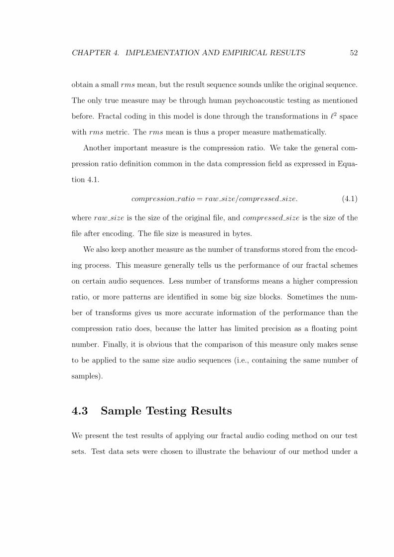
CHAPTER 4. IMPLEMENTATION AND EMPIRICAL RESULTS 52
obtain a small rms mean, but the result sequence sounds unlike the original sequence.
The only true measure may be through human psychoacoustic testing as mentioned
before. Fractal coding in this model is done through the transformations in `2 space
with rms metric. The rms mean is thus a proper measure mathematically.
Another important measure is the compression ratio. We take the general com-
pression ratio definition common in the data compression field as expressed in Equa-
tion 4.1.
compression ratio = raw size/compressed size. (4.1)
where raw size is the size of the original file, and compressed size is the size of the
file after encoding. The file size is measured in bytes.
We also keep another measure as the number of transforms stored from the encod-
ing process. This measure generally tells us the performance of our fractal schemes
on certain audio sequences. Less number of transforms means a higher compression
ratio, or more patterns are identified in some big size blocks. Sometimes the num-
ber of transforms gives us more accurate information of the performance than the
compression ratio does, because the latter has limited precision as a floating point
number. Finally, it is obvious that the comparison of this measure only makes sense
to be applied to the same size audio sequences (i.e., containing the same number of
samples).
4.3 Sample Testing Results
We present the test results of applying our fractal audio coding method on our test
sets. Test data sets were chosen to illustrate the behaviour of our method under a
CHAPTER 4. IMPLEMENTATION AND EMPIRICAL RESULTS 53
variety of conditions.
4.3.1 Tolerance
The domain-range mapping error tolerance erms is a very critical parameter domi-
nating the compression ratio as well as the encoding quality in our fractal scheme.
Intuitively, the bigger the erms value, the higher the compression ratio that can be
achieved, because more mappings can be accepted for the large size range blocks, and
thus fewer transforms need to be stored. On the other hand, a smaller erms value gives
a better encoding quality. Note that we use the rms mean to measure the quality of
encoding.
The experiment on erms is built upon other fractal coding experimental results
with images. We fix the bit allocation using Fisher’s optimal results [5](ch.3) on
fractal image coding (i.e., si = 5 and oi = 7), and allow erms to be varied in the set:
{4, 5, 6, 7, 8, 9}. Throughout the study, we try to find a good tolerance value which
balances the compression ratio and encoding quality. Also, the study shall give us
some idea of the compression ratio range on applying fractal coding to audio data in
general.
CHAPTER 4. IMPLEMENTATION AND EMPIRICAL RESULTS 54
0
1
2
3
4
5
6
7
4 5 6 7 8 9
Tolerance
Com
pres
sion
Rat
io
myside.wav
bee5.wav
dogjingl.wav
saxophone.wav
Figure 4.3: The compression ratio versus the erms with different WAVE files.
0
4
4 5 6 7 8 9
Tolerance
rms
Mea
n
myside.wavbee5.wavdogjingl.wavsaxophone.wav
Figure 4.4: The rms mean versus the erms with different WAVE files.
As is to be expected, Figure 4.3 and Figure 4.44 show that a bigger erms value leads
4We demonstrate four WAVE files results with one from each of the four test categories in bothfigures.
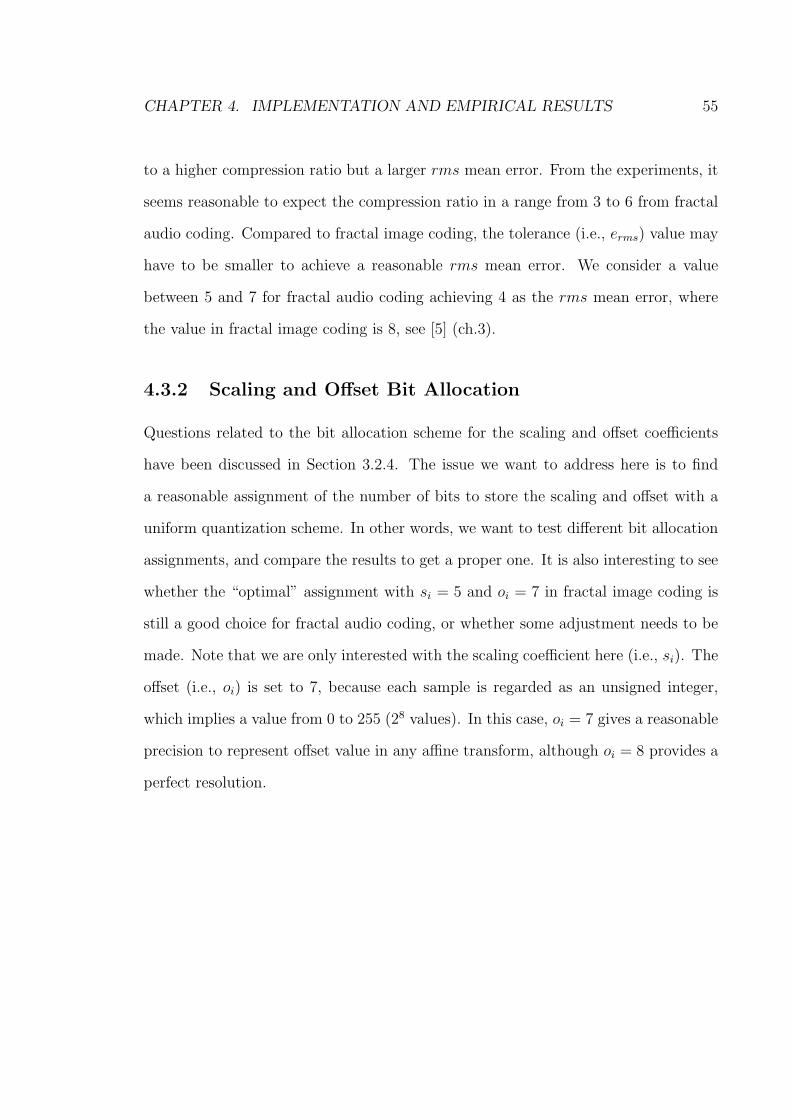
CHAPTER 4. IMPLEMENTATION AND EMPIRICAL RESULTS 55
to a higher compression ratio but a larger rms mean error. From the experiments, it
seems reasonable to expect the compression ratio in a range from 3 to 6 from fractal
audio coding. Compared to fractal image coding, the tolerance (i.e., erms) value may
have to be smaller to achieve a reasonable rms mean error. We consider a value
between 5 and 7 for fractal audio coding achieving 4 as the rms mean error, where
the value in fractal image coding is 8, see [5] (ch.3).
4.3.2 Scaling and Offset Bit Allocation
Questions related to the bit allocation scheme for the scaling and offset coefficients
have been discussed in Section 3.2.4. The issue we want to address here is to find
a reasonable assignment of the number of bits to store the scaling and offset with a
uniform quantization scheme. In other words, we want to test different bit allocation
assignments, and compare the results to get a proper one. It is also interesting to see
whether the “optimal” assignment with si = 5 and oi = 7 in fractal image coding is
still a good choice for fractal audio coding, or whether some adjustment needs to be
made. Note that we are only interested with the scaling coefficient here (i.e., si). The
offset (i.e., oi) is set to 7, because each sample is regarded as an unsigned integer,
which implies a value from 0 to 255 (28 values). In this case, oi = 7 gives a reasonable
precision to represent offset value in any affine transform, although oi = 8 provides a
perfect resolution.
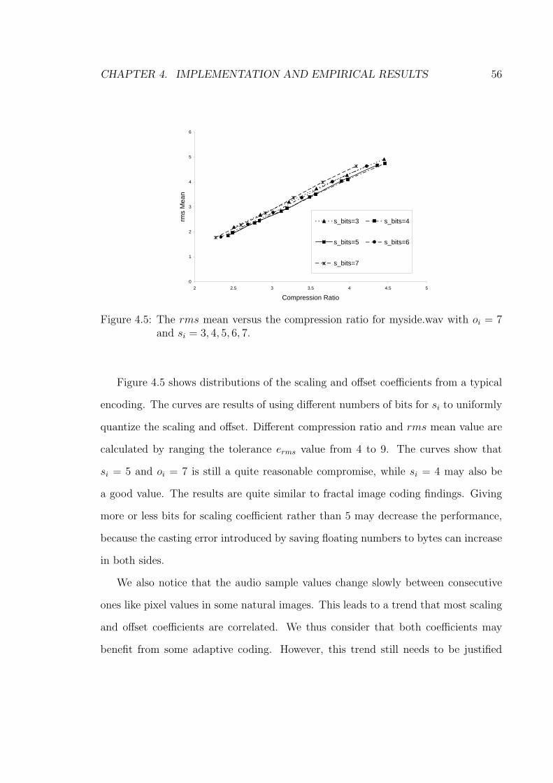
CHAPTER 4. IMPLEMENTATION AND EMPIRICAL RESULTS 56
0
1
2
3
4
5
6
2 2.5 3 3.5 4 4.5 5
Compression Ratio
rms
Mea
n
s_bits=3 s_bits=4
s_bits=5 s_bits=6
s_bits=7
Figure 4.5: The rms mean versus the compression ratio for myside.wav with oi = 7and si = 3, 4, 5, 6, 7.
Figure 4.5 shows distributions of the scaling and offset coefficients from a typical
encoding. The curves are results of using different numbers of bits for si to uniformly
quantize the scaling and offset. Different compression ratio and rms mean value are
calculated by ranging the tolerance erms value from 4 to 9. The curves show that
si = 5 and oi = 7 is still a quite reasonable compromise, while si = 4 may also be
a good value. The results are quite similar to fractal image coding findings. Giving
more or less bits for scaling coefficient rather than 5 may decrease the performance,
because the casting error introduced by saving floating numbers to bytes can increase
in both sides.
We also notice that the audio sample values change slowly between consecutive
ones like pixel values in some natural images. This leads to a trend that most scaling
and offset coefficients are correlated. We thus consider that both coefficients may
benefit from some adaptive coding. However, this trend still needs to be justified
CHAPTER 4. IMPLEMENTATION AND EMPIRICAL RESULTS 57
through further experiments on more audio data.
4.3.3 Audio Type
Our testing audio set consists of different types of audio data (see Appendix A for
descriptions), which has been stated in Section 4.2.1. Intuitively, the fractal audio
scheme may have different performances on different types of audio data. We have
done some experiments to explore whether the performance is related with the type
of audio data, or whether the fractal audio scheme is suitable on one type more than
others.
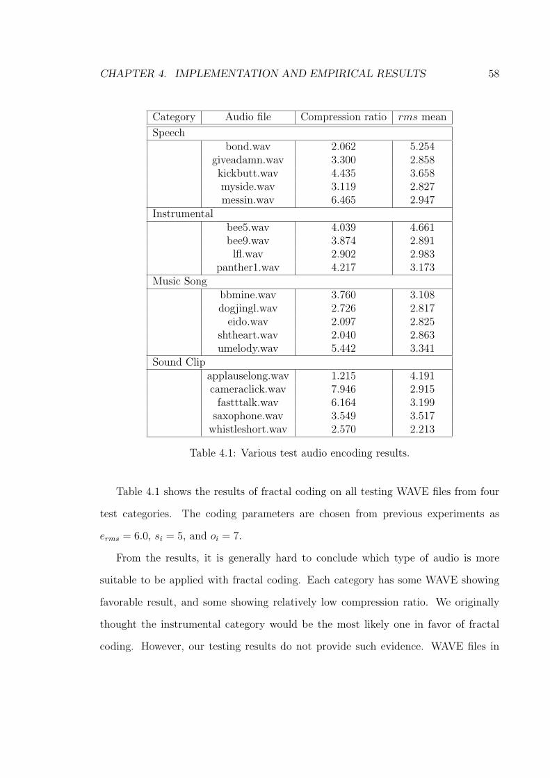
CHAPTER 4. IMPLEMENTATION AND EMPIRICAL RESULTS 58
Category Audio file Compression ratio rms mean
Speechbond.wav 2.062 5.254
giveadamn.wav 3.300 2.858kickbutt.wav 4.435 3.658myside.wav 3.119 2.827messin.wav 6.465 2.947
Instrumentalbee5.wav 4.039 4.661bee9.wav 3.874 2.891lfl.wav 2.902 2.983
panther1.wav 4.217 3.173Music Song
bbmine.wav 3.760 3.108dogjingl.wav 2.726 2.817
eido.wav 2.097 2.825shtheart.wav 2.040 2.863umelody.wav 5.442 3.341
Sound Clipapplauselong.wav 1.215 4.191cameraclick.wav 7.946 2.915
fastttalk.wav 6.164 3.199saxophone.wav 3.549 3.517
whistleshort.wav 2.570 2.213
Table 4.1: Various test audio encoding results.
Table 4.1 shows the results of fractal coding on all testing WAVE files from four
test categories. The coding parameters are chosen from previous experiments as
erms = 6.0, si = 5, and oi = 7.
From the results, it is generally hard to conclude which type of audio is more
suitable to be applied with fractal coding. Each category has some WAVE showing
favorable result, and some showing relatively low compression ratio. We originally
thought the instrumental category would be the most likely one in favor of fractal
coding. However, our testing results do not provide such evidence. WAVE files in
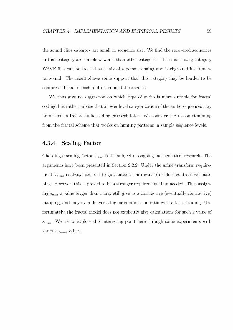
CHAPTER 4. IMPLEMENTATION AND EMPIRICAL RESULTS 59
the sound clips category are small in sequence size. We find the recovered sequences
in that category are somehow worse than other categories. The music song category
WAVE files can be treated as a mix of a person singing and background instrumen-
tal sound. The result shows some support that this category may be harder to be
compressed than speech and instrumental categories.
We thus give no suggestion on which type of audio is more suitable for fractal
coding, but rather, advise that a lower level categorization of the audio sequences may
be needed in fractal audio coding research later. We consider the reason stemming
from the fractal scheme that works on hunting patterns in sample sequence levels.
4.3.4 Scaling Factor
Choosing a scaling factor smax is the subject of ongoing mathematical research. The
arguments have been presented in Section 2.2.2. Under the affine transform require-
ment, smax is always set to 1 to guarantee a contractive (absolute contractive) map-
ping. However, this is proved to be a stronger requirement than needed. Thus assign-
ing smax a value bigger than 1 may still give us a contractive (eventually contractive)
mapping, and may even deliver a higher compression ratio with a faster coding. Un-
fortunately, the fractal model does not explicitly give calculations for such a value of
smax. We try to explore this interesting point here through some experiments with
various smax values.
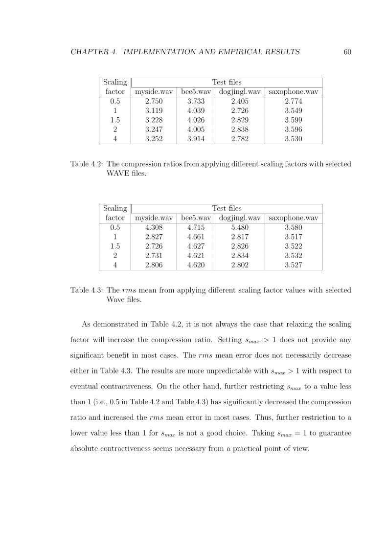
CHAPTER 4. IMPLEMENTATION AND EMPIRICAL RESULTS 60
Scaling Test filesfactor myside.wav bee5.wav dogjingl.wav saxophone.wav0.5 2.750 3.733 2.405 2.7741 3.119 4.039 2.726 3.549
1.5 3.228 4.026 2.829 3.5992 3.247 4.005 2.838 3.5964 3.252 3.914 2.782 3.530
Table 4.2: The compression ratios from applying different scaling factors with selectedWAVE files.
Scaling Test filesfactor myside.wav bee5.wav dogjingl.wav saxophone.wav0.5 4.308 4.715 5.480 3.5801 2.827 4.661 2.817 3.517
1.5 2.726 4.627 2.826 3.5222 2.731 4.621 2.834 3.5324 2.806 4.620 2.802 3.527
Table 4.3: The rms mean from applying different scaling factor values with selectedWave files.
As demonstrated in Table 4.2, it is not always the case that relaxing the scaling
factor will increase the compression ratio. Setting smax > 1 does not provide any
significant benefit in most cases. The rms mean error does not necessarily decrease
either in Table 4.3. The results are more unpredictable with smax > 1 with respect to
eventual contractiveness. On the other hand, further restricting smax to a value less
than 1 (i.e., 0.5 in Table 4.2 and Table 4.3) has significantly decreased the compression
ratio and increased the rms mean error in most cases. Thus, further restriction to a
lower value less than 1 for smax is not a good choice. Taking smax = 1 to guarantee
absolute contractiveness seems necessary from a practical point of view.
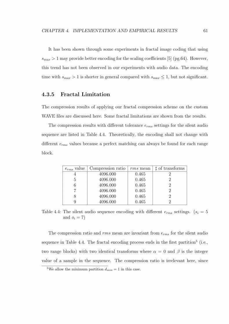
CHAPTER 4. IMPLEMENTATION AND EMPIRICAL RESULTS 61
It has been shown through some experiments in fractal image coding that using
smax > 1 may provide better encoding for the scaling coefficients [5] (pg.64). However,
this trend has not been observed in our experiments with audio data. The encoding
time with smax > 1 is shorter in general compared with smax ≤ 1, but not significant.
4.3.5 Fractal Limitation
The compression results of applying our fractal compression scheme on the custom
WAVE files are discussed here. Some fractal limitations are shown from the results.
The compression results with different tolerance erms settings for the silent audio
sequence are listed in Table 4.4. Theoretically, the encoding shall not change with
different erms values because a perfect matching can always be found for each range
block.
erms value Compression ratio rms mean ] of transforms4 4096.000 0.465 25 4096.000 0.465 26 4096.000 0.465 27 4096.000 0.465 28 4096.000 0.465 29 4096.000 0.465 2
Table 4.4: The silent audio sequence encoding with different erms settings. (si = 5and oi = 7)
The compression ratio and rms mean are invariant from erms for the silent audio
sequence in Table 4.4. The fractal encoding process ends in the first partition5 (i.e.,
two range blocks) with two identical transforms where α = 0 and β is the integer
value of a sample in the sequence. The compression ratio is irrelevant here, since
5We allow the minimum partition dmin = 1 in this case.
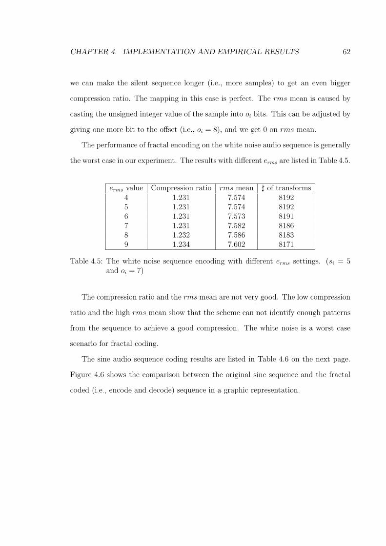
CHAPTER 4. IMPLEMENTATION AND EMPIRICAL RESULTS 62
we can make the silent sequence longer (i.e., more samples) to get an even bigger
compression ratio. The mapping in this case is perfect. The rms mean is caused by
casting the unsigned integer value of the sample into oi bits. This can be adjusted by
giving one more bit to the offset (i.e., oi = 8), and we get 0 on rms mean.
The performance of fractal encoding on the white noise audio sequence is generally
the worst case in our experiment. The results with different erms are listed in Table 4.5.
erms value Compression ratio rms mean ] of transforms4 1.231 7.574 81925 1.231 7.574 81926 1.231 7.573 81917 1.231 7.582 81868 1.232 7.586 81839 1.234 7.602 8171
Table 4.5: The white noise sequence encoding with different erms settings. (si = 5and oi = 7)
The compression ratio and the rms mean are not very good. The low compression
ratio and the high rms mean show that the scheme can not identify enough patterns
from the sequence to achieve a good compression. The white noise is a worst case
scenario for fractal coding.
The sine audio sequence coding results are listed in Table 4.6 on the next page.
Figure 4.6 shows the comparison between the original sine sequence and the fractal
coded (i.e., encode and decode) sequence in a graphic representation.
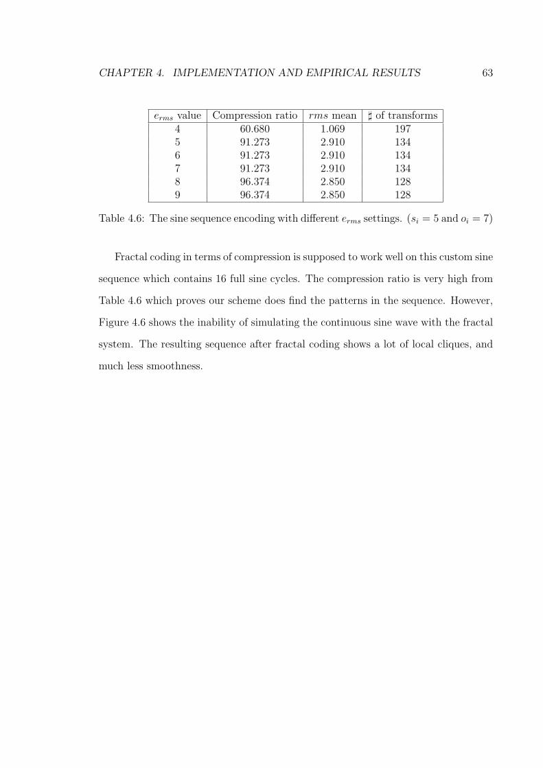
CHAPTER 4. IMPLEMENTATION AND EMPIRICAL RESULTS 63
erms value Compression ratio rms mean ] of transforms4 60.680 1.069 1975 91.273 2.910 1346 91.273 2.910 1347 91.273 2.910 1348 96.374 2.850 1289 96.374 2.850 128
Table 4.6: The sine sequence encoding with different erms settings. (si = 5 and oi = 7)
Fractal coding in terms of compression is supposed to work well on this custom sine
sequence which contains 16 full sine cycles. The compression ratio is very high from
Table 4.6 which proves our scheme does find the patterns in the sequence. However,
Figure 4.6 shows the inability of simulating the continuous sine wave with the fractal
system. The resulting sequence after fractal coding shows a lot of local cliques, and
much less smoothness.
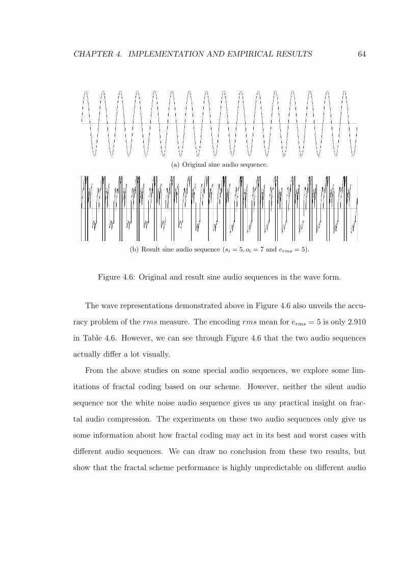
CHAPTER 4. IMPLEMENTATION AND EMPIRICAL RESULTS 64
(a) Original sine audio sequence.
(b) Result sine audio sequence (si = 5, oi = 7 and erms = 5).
Figure 4.6: Original and result sine audio sequences in the wave form.
The wave representations demonstrated above in Figure 4.6 also unveils the accu-
racy problem of the rms measure. The encoding rms mean for erms = 5 is only 2.910
in Table 4.6. However, we can see through Figure 4.6 that the two audio sequences
actually differ a lot visually.
From the above studies on some special audio sequences, we explore some lim-
itations of fractal coding based on our scheme. However, neither the silent audio
sequence nor the white noise audio sequence gives us any practical insight on frac-
tal audio compression. The experiments on these two audio sequences only give us
some information about how fractal coding may act in its best and worst cases with
different audio sequences. We can draw no conclusion from these two results, but
show that the fractal scheme performance is highly unpredictable on different audio
CHAPTER 4. IMPLEMENTATION AND EMPIRICAL RESULTS 65
sequences. The result on the sine audio sequence on the other hand supports the the-
oretical hypothesis that fractals are not able to simulate continuous functions. This
disadvantage is a major challenge when trying to apply fractal coding on audio data.
4.3.6 Other Issues
Our implementation allows us to experiment on some other issues related to fractal
coding, such as domain pool selection, domain classification, and postprocessing.
Again, many issues have been studied in fractal image coding. However, we do not
present the experimental results on those issues here, because most of them belong
to a later stage of development, and fractal audio coding research is still in its early
period.
Among those issues, postprocessing is an interesting topic which may be further
studied for the reason that some constant background noise is observed from the audio
sequences after fractal coding. We suspect a strong block artifact problem from our
fractal audio coding scheme. Unfortunately, our simple postprocessing method of
averaging the edges between two blocks does not seem to work well to solve this
problem. We suspect that some extra work needs to be done with our scheme to
solve this problem.
Preprocessing is an issue that we do not address in our experiment. It has been
shown to be very useful in this field by taking some transform technique such as a
wavelet transform, as reviewed in Section 3.3. Preprocessing may also be a method to
detect whether fractal coding can be applied with the given audio sequences. A trend
that has been observed from our empirical results is that it does not seem appropriate
to apply fractal coding on small audio sequences. In most of those cases, the loss from
CHAPTER 4. IMPLEMENTATION AND EMPIRICAL RESULTS 66
applying fractal coding is significant and the quality of recovery is very bad.
4.4 Conclusion
In this chapter, we provided our implementation of a fractal audio coding scheme
and some empirical results from our experiment with various audio data. We shall
conclude based on our results, and give suggestion for future studies on this subject.
• The compression ratio from applying fractal audio coding may be in a range
from 3 to 6 in general, with a tolerance value between 5 and 7.
• Comparing with fractal image coding, fractal audio coding requires more pre-
cision on mapping (i.e., smaller erms value). The compression ratio is much
lower than in the image case, because the weakness of fractal system’s ability
of simulating continuous functions. Fractal coding may thus not be appropriate
to be directly applied on audio.
• Unlike with images, it is in general hard to conclude which type of audio is
more suitable to be a fractal subject. Our results show no strong support for
any type of audio. Furthermore, fractal coding’s highly unpredictability has
been demonstrated through our experiment with some custom audio sequences.
• Under the affine transformation assumption, the scaling factor smax value is
still better to be 1 to guarantee the absolute contractiveness. Values that are
greater than 1 give more unpredictable results, and are thus unreliable.
• Fractal coding does not seem to be a good choice for small audio sequences (in
terms of number of samples). The loss from applying fractal coding on those
CHAPTER 4. IMPLEMENTATION AND EMPIRICAL RESULTS 67
sequences is usually significant.
• Preprocessing can be considered to improve fractal audio coding. Good pre-
processing shall help to break the audio sequence’s continuity in order to make
the fractal system work well later. Preprocessing can also be used to decide
whether fractal coding is applicable for a particular sequence.
• It seems that the block artifact produces some background noise through our
fractal audio coding scheme. The same problem is solved in fractal image coding
allowing range block to overlap, or taking wavelet transform as the preprocessing
step. The latter approach has been taken by [25]. But no discussion has been
posted regarding the block artifact problem on fractal audio coding yet.
Chapter 5
Discussion
5.1 Summary and Conclusion
This thesis presents a quick overview on fractal coding. We review fractal coding
development through the main literature on this subject. Fractal theory is provided
in Chapter 2 with some focus on the fractal audio model. We implement a fractal
audio coding scheme to carry out our experiment described in Chapter 4. Some
aspects of fractal coding have been practised through empirical studies on various
audio sequences.
Ultimately, our experience suggests that fractal coding may not be good enough
to stand alone in audio compression, while fractal systems are still of a great interest
in the compression field. As stated at the beginning of this thesis, our purpose to
carry out this research on fractal coding is an attempt to extend fractal coding to
audio data, and explore how the fractal system performs under its audio model. Our
study tries to contribute to future fractal audio coding research, or in general fractal
system applications with experimental results and evidence.
68
CHAPTER 5. DISCUSSION 69
5.2 Recommendations for Future Work
Through a large amount of studies on fractal image coding, it has been demonstrated
that fractal coding can be nicely integrated into the framework of conventional com-
pression techniques such as vector quantization and transform methods. The future
aspect on fractals seems to focus on this kind of integration. Built upon the success of
applying wavelets in image compression, hybrid fractal wavelet image coding schemes
are introduced in [4] [7] [23]. This idea has also been practised in fractal audio coding
too [25]. This direction may also lead to a potential success on applying fractal audio
coding in practise.
In terms of improvement, preprocessing may be promising. A preprocessing step
can be used to break the continuity in audio sequences, which may provide a way of
compensating for the shortcomings of fractal systems. In fractal image coding, we
have seen the applications with wavelets and DCT to supply this function. We expect
that the same concept may be applicable in fractal audio coding too.
Specific to audio data, a proper classification shall help the compression scheme
greatly. Fractal audio coding can clearly take the advantage of the classification
to improve the mapping quality as well as the searching efficiency. However, the
classification of audio data is probably a more general topic to be concerned, which
may be addressed from other different perspectives.
Bibliography
[1] M. Tonkelowitz A. Patel and M. Vernal. Lossless sound compression using dis-
crete wavelet transform. Department of Electrical Engineering and Computer
Science, Harvard University, January 2002.
[2] A. Bernat. Which partition scheme for what image? partitioned iterated function
systems for fractal image compression. Master’s thesis, Queen’s University, ON,
Canada, January 2001.
[3] J. A. Nicholls D. L.Wilson and D. M. Monro. Rate buffered fractal video. In
Proceedings ICASSP-94, volume 5, pages 505–508, Adelaide, Australia, April
1994. IEEE international Conference on Acoustics, Speech and Signal Processing.
[4] G. M. Davis. A wavelet-based analysis of fractal image compression. IEEE
Transactions on Image Processing, 7(2):141–154, February 1998.
[5] Y. Fisher. Fractal Image Compression: Theory and Application. Springer Verlag,
New York, USA, 1995.
[6] A. Gersho and R. M. Gray. Vector Quantization and Signal Compression, Com-
munications and Information Theory. Kluwer Academic Publishers, Norwell,
MA, USA, 1992.
70
BIBLIOGRAPHY 71
[7] D. Malah H. Krupnik and E. Karnin. Fractal representation of image via the dis-
crete wavelet transform. In 18th IEEE Convention of Electrical and Electronics
Engineers in Israel, pages 1089–1100, Tel Aviv, Israel, March 1995.
[8] W. M. Hartmann. Signals, Sound, and Sensation. AIP Press, 1 edition, January
1997.
[9] A. E. Jacquin. Image coding based on a fractal theory of iterated contractive
image transformations. IEEE Transactions on Image Processing, 1(1):18–30,
January 1992.
[10] T. Voye K. U. Barthel and P. Noll. Improved fractal image coding. In Proceed-
ings PCS’93, Lausanne, Switzerland, March 1993. International Picture Coding
Symposium.
[11] N. Lu. Fractal Imaging. Academic Press, San Diego, CA, USA, 1997.
[12] W. K. Cheung M. L. Po, Y. Zhang and H. C. Cheung. A novel subtree par-
titioning algorithm for wavelet-based fractal image coding. In D. Saupe and
R. Hamzaoui, editors, Proceedings of ICASSP’98, volume 5, Seattle, Washington,
USA, 1998. International Conference on Acoustics, Speech, and Signal Process-
ing.
[13] G. S. Mallat. Multiresolution approximations and wavelet orthogonal bases of
`2(r). Transactions of American Mathematical Society, 315:69–87, 1989a.
[14] G. S. Mallat. A theory of multiresolution signal decomposition: the wavelet rep-
resentation. IEEE Transactions on Pattern Analysis and Machine Intelligence,
11:674–693, July 1989b.
BIBLIOGRAPHY 72
[15] G. Melnikov and A. K. Katsaggelos. A jointly optimal Fractal/DCT compression
scheme. IEEE Transactions on Multimedia, 4(4):413–422, December 2002.
[16] M. Nelson and J.-L. Gailly. The Data Compression Book. M&T Books, New
York, USA, 2nd edition, 1996.
[17] M. Muller R. Hamzaoui and D. Saupe. VQ-enhanced fractal image compression.
In Proceedings of ICIP’96, volume I, pages 153–156, Lausanne, Switzerland,
September 1996. IEEE International Conference on Image Processing.
[18] R. M. Rao and A. S. Bopardikar. Wavelet Transforms: Introduction to Theory
and Applications. Addison Wesley Longman, MA, USA, 1998.
[19] H. L. Resnikoff and Jr. R. O. Wells. Wavelet Analysis: The Scalable Structure
of Information. Springer Verlag, New York, USA, 1998.
[20] E. Reusens. Overlapped adaptive partitioning for image coding based on the
theory of iterated functions systems. In Proceedings ICASSP-94, volume 5,
pages 569–572, Adelaide, Australia, April 1994. IEEE international Conference
on Acoustics, Speech and Signal Processing.
[21] M. Ruhl and H. Hartenstein. Optimal fractal coding is np-hard. In Proceed-
ings of DCC’97, pages 261–270, Snowbird, UT, USA, March 1997. IEEE Data
Compression Conference.
[22] B. Simon. Explicit link between local fractal transform and multiresolution trans-
form. In Proceedings of ICIP’95, volume I, pages 278–281, Washington, D.C.,
USA, October 1995. IEEE International Conference on Image Processing.
BIBLIOGRAPHY 73
[23] A. van de Walle. Merging fractal image compression and wavelet transform
methods. In Proceedings of the NATO Advanced Study Institute, pages 8–17,
Trondheim, Norway, July 1995.
[24] A. van de Walle. Relating fractal image compression to transform methods.
Master’s thesis, University of Waterloo, Waterloo, Canada, 1995.
[25] R. A. Wannamaker and E. R. Vrscay. Fractal wavelet compression of audio
signals. J. Audio Eng. Soc., 45, July,August 1997.
[26] B. Wohlberg and G. de Jager. A review of the fractal image coding literature.
IEEE Transaction on Image Processing, 8(12):1716–1729, December 1999.
[27] D. J. Wright. Dynamical systems and fractals lecture notes.
http://www.math.okstate.edu/mathdept/dynamics/lecnotes/lecnotes.html,
August 1996.
[28] D. N. Rogovin Y. Fisher and T.-P. J. Shen. Comparison of fractal methods with
discrete cosine transform (DCT) and wavelets. In S.-S. Chen, editor, SPIE Pro-
ceedings, volume 2304, pages 132–143, San Diego, CA, USA, July 1994. Neural
and Stochastic Methods in Image and Signal Processing III.
[29] D. N. Rogovin Y. Fisher and T.-P. J. Shen. Fractal (self-vq) encoding of video
sequences. In A. K. Katsaggelos, editor, SPIE Proceedings, volume 2308, pages
1359–1370, Chicago, IL, USA, September 1994. Visual Communications and Im-
age Processing ’94.
[30] E. W. Jacobs Y. Fisher and R. D. Boss. Fractal image compression using iterated
transform. Image and Text Compression, pages 35–61, 1992.
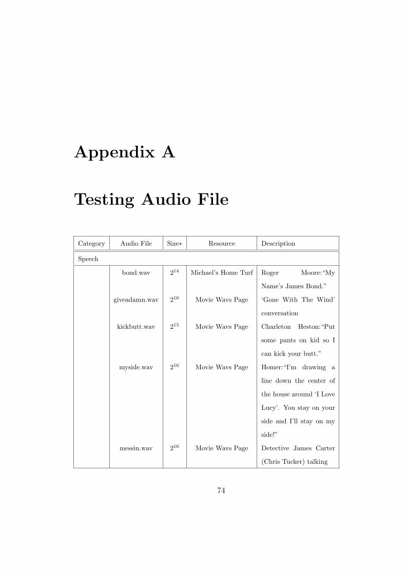
Appendix A
Testing Audio File
Category Audio File Size∗ Resource Description
Speech
bond.wav 214 Michael’s Home Turf Roger Moore:“My
Name’s James Bond.”
giveadamn.wav 216 Movie Wavs Page ‘Gone With The Wind’
conversation
kickbutt.wav 215 Movie Wavs Page Charleton Heston:“Put
some pants on kid so I
can kick your butt.”
myside.wav 216 Movie Wavs Page Homer:“I’m drawing a
line down the center of
the house around ‘I Love
Lucy’. You stay on your
side and I’ll stay on my
side!”
messin.wav 216 Movie Wavs Page Detective James Carter
(Chris Tucker) talking
74
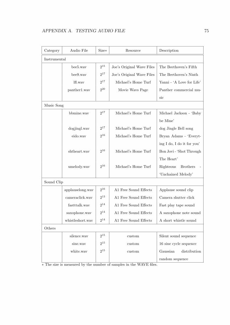
APPENDIX A. TESTING AUDIO FILE 75
Category Audio File Size∗ Resource Description
Instrumental
bee5.wav 215 Joe’s Original Wave Files The Beethoven’s Fifth
bee9.wav 217 Joe’s Original Wave Files The Beethoven’s Ninth
lfl.wav 217 Michael’s Home Turf Yanni - ‘A Love for Life’
panther1.wav 220 Movie Wavs Page Panther commercial mu-
sic
Music Song
bbmine.wav 217 Michael’s Home Turf Michael Jackson - ‘Baby
be Mine’
dogjingl.wav 217 Michael’s Home Turf dog Jingle Bell song
eido.wav 216 Michael’s Home Turf Bryan Adams - ‘Everyt-
ing I do, I do it for you’
shtheart.wav 216 Michael’s Home Turf Bon Jovi - ‘Shot Through
The Heart’
umelody.wav 216 Michael’s Home Turf Righteous Brothers -
‘Unchained Melody’
Sound Clip
applauselong.wav 216 A1 Free Sound Effects Applause sound clip
cameraclick.wav 213 A1 Free Sound Effects Camera shutter click
fastttalk.wav 214 A1 Free Sound Effects Fast play tape sound
saxophone.wav 214 A1 Free Sound Effects A saxophone note sound
whistleshort.wav 214 A1 Free Sound Effects A short whistle sound
Others
silence.wav 215 custom Silent sound sequence
sine.wav 215 custom 16 sine cycle sequence
white.wav 215 custom Gaussian distribution
random sequence∗ The size is measured by the number of samples in the WAVE files.
Appendix B
WAVE PCM Format
There are various formats for storing digital sound files. In computing, the sound is normally
digitized through sampling, on which we take a sample of the wave frequencies that occur in the
analog sound. So the more samples we take when we digitize, the higher fidelity of the digitized
sound will be to the analog original. One sample is a certain fixed number of bits, normally 8-bit
or 16-bit, with each bit setting to “on”(1) or “off”(0). The number of the bits per sample is the
bit resolution. The sample rate is specified in kilohertz (kHz), that is, in thousands of samples per
second. The highest possible pitch in the sound is equal to one half of the sample rate. So on a music
CD, where sound is sampled at 44.1 kHz, the highest pitch possible is 22.050 kHz, which is also the
top of the human hearing range. Audio sampling is also called Pulse Code Modulation (PCM).
The digital sound format we are interested in this thesis is the WAVE file format, which was
created by Microsoft and IBM. The WAVE file format directly stores the samples from ADPCM
(analog-to-digital PCM ) supporting a variety of bit resolution, sample rates, and channels of audio. It
also allows some different compression methods. However, we are only looking for the uncompressed
WAVE files as our raw data to apply our compression scheme here.
Data Organization
The WAVE file format uses the Microsoft version of the Electronic Arts Interchange File Format
method for storing data in“chunks”. All data is stored in 8-bit bytes, arranged in Intel 80x86 (i.e.
76
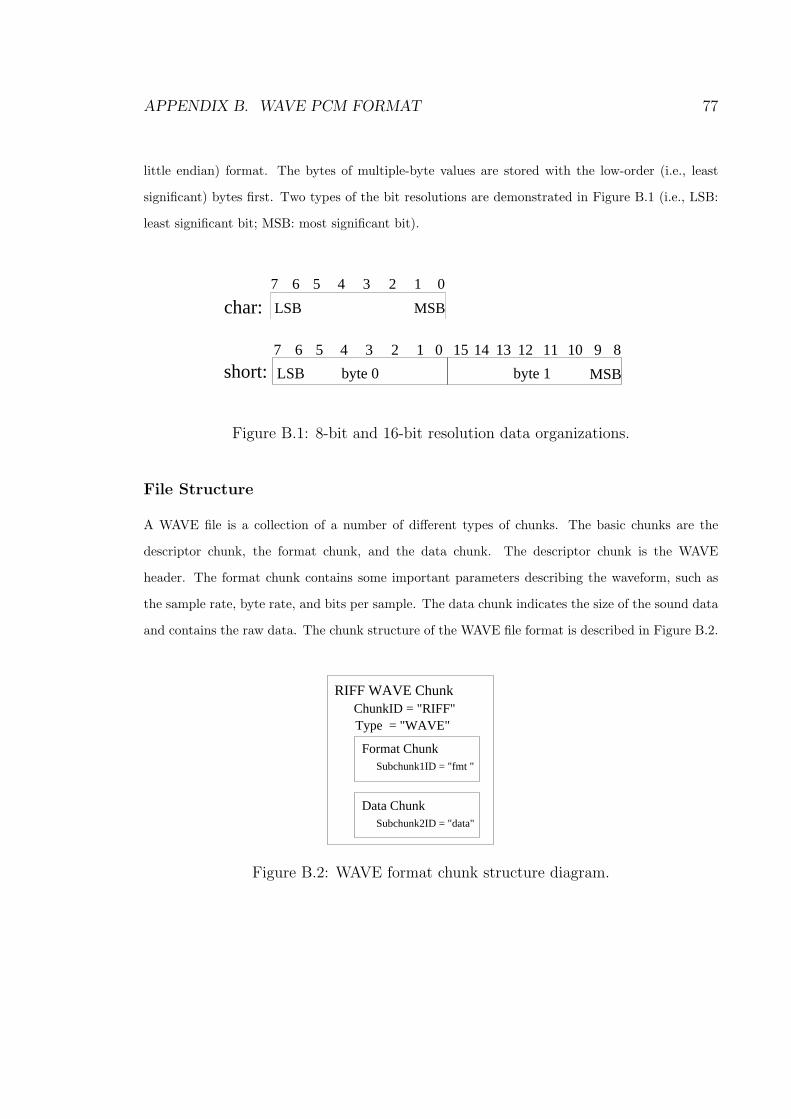
APPENDIX B. WAVE PCM FORMAT 77
little endian) format. The bytes of multiple-byte values are stored with the low-order (i.e., least
significant) bytes first. Two types of the bit resolutions are demonstrated in Figure B.1 (i.e., LSB:
least significant bit; MSB: most significant bit).
01234567
MSBLSBchar:
1234567 150 891011121314
LSB MSBbyte 1byte 0short:
Figure B.1: 8-bit and 16-bit resolution data organizations.
File Structure
A WAVE file is a collection of a number of different types of chunks. The basic chunks are the
descriptor chunk, the format chunk, and the data chunk. The descriptor chunk is the WAVE
header. The format chunk contains some important parameters describing the waveform, such as
the sample rate, byte rate, and bits per sample. The data chunk indicates the size of the sound data
and contains the raw data. The chunk structure of the WAVE file format is described in Figure B.2.
RIFF WAVE ChunkChunkID = "RIFF"Type = "WAVE"
Format Chunk
Data Chunk
Subchunk1ID = "fmt "
Subchunk2ID = "data"
Figure B.2: WAVE format chunk structure diagram.
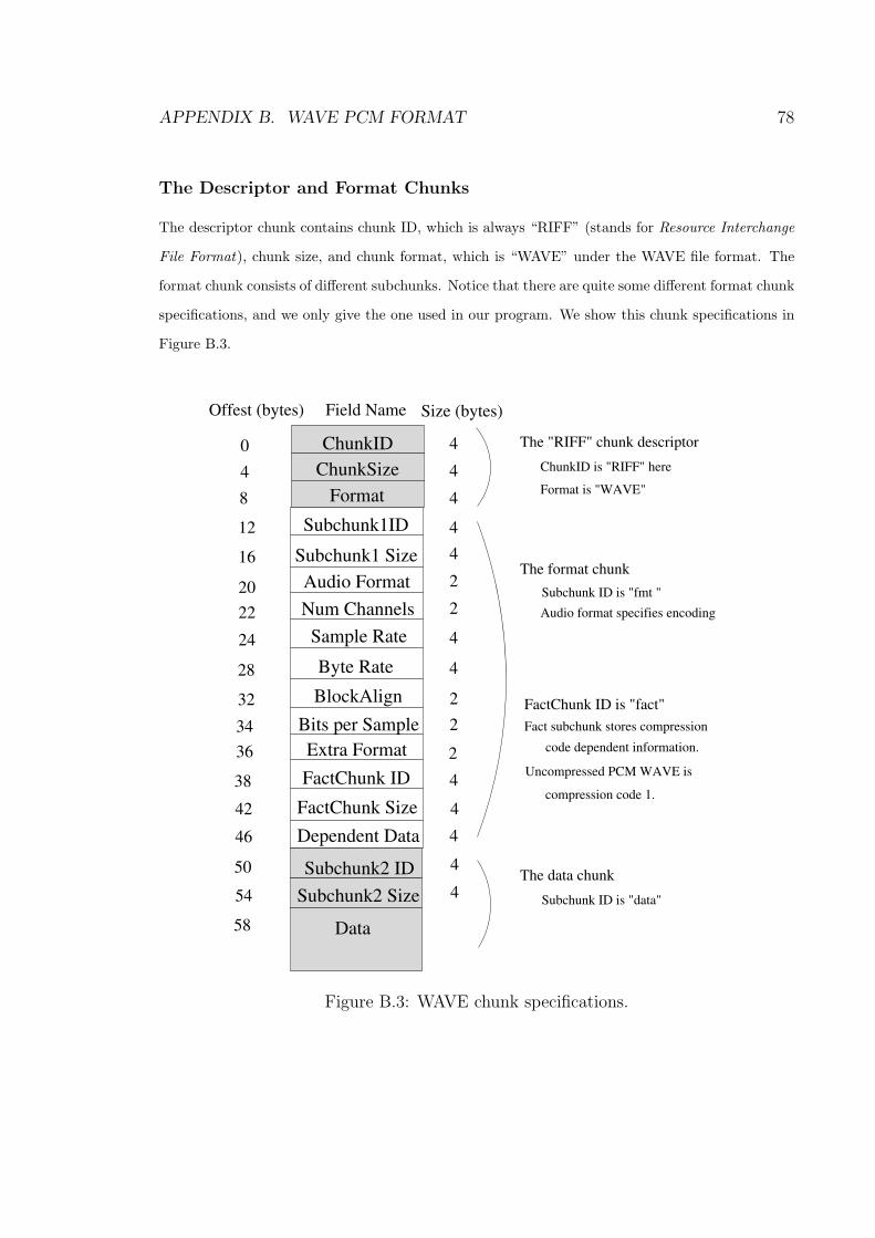
APPENDIX B. WAVE PCM FORMAT 78
The Descriptor and Format Chunks
The descriptor chunk contains chunk ID, which is always “RIFF” (stands for Resource Interchange
File Format), chunk size, and chunk format, which is “WAVE” under the WAVE file format. The
format chunk consists of different subchunks. Notice that there are quite some different format chunk
specifications, and we only give the one used in our program. We show this chunk specifications in
Figure B.3.
code dependent information.
Uncompressed PCM WAVE is
compression code 1.
Fact subchunk stores compression
The format chunk
The "RIFF" chunk descriptor
The data chunk
ChunkID is "RIFF" here
Format is "WAVE"
Subchunk ID is "fmt "
Subchunk ID is "data"
Audio format specifies encoding
FactChunk ID is "fact"
Offest (bytes) Field Name Size (bytes)
4
0
8
Subchunk1ID
Format
ChunkSize
Sample Rate
Byte Rate
Subchunk1 Size
Audio Format
Num Channels
4
4
4
412
16
Bits per Sample
BlockAlign
2
2
4
4
22
20
24
FactChunk Size
FactChunk ID
Dependent Data
Extra Format
4
2
Subchunk2 Size
Data
4
2
2
4
4
4
4
28
32
34
36
38
50
54
46
42
ChunkID
Subchunk2 ID
58
Figure B.3: WAVE chunk specifications.
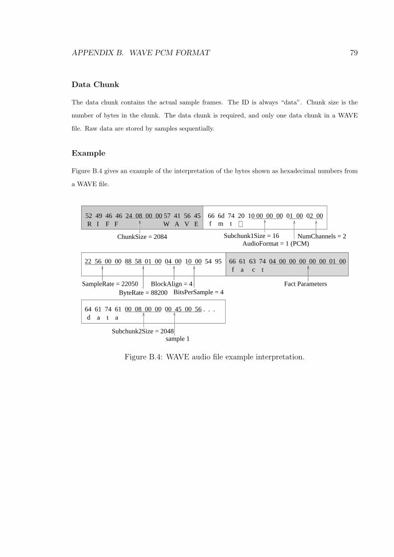
APPENDIX B. WAVE PCM FORMAT 79
Data Chunk
The data chunk contains the actual sample frames. The ID is always “data”. Chunk size is the
number of bytes in the chunk. The data chunk is required, and only one data chunk in a WAVE
file. Raw data are stored by samples sequentially.
Example
Figure B.4 gives an example of the interpretation of the bytes shown as hexadecimal numbers from
a WAVE file.
R I F F W A V E52 49 46 46 24 08 00 00 57 41 56 45 66 6d 74 20 10 00 00 00 01 00 02 00
f m t
ChunkSize = 2084 Subchunk1Size = 16AudioFormat = 1 (PCM)
NumChannels = 2
SampleRate = 22050 BlockAlign = 4BitsPerSample = 4ByteRate = 88200
22 56 00 00 88 58 01 00 04 00 10 00 54 95 66 61 63 74 04 00 00 00 00 00 01 00f a c t
Fact Parameters
64 61 74 61 00 08 00 00 00 45 00 56 . . .d a t a
Subchunk2Size = 2048sample 1
Figure B.4: WAVE audio file example interpretation.


![AUDIO CODING STANDARDS - mp3-tech.org · The advances of audio coding techniques and the ... 1992], and the Dolby AC-3 [Todd, 1994] algorithm. “Audio Coding Standards,” A chapter](https://img.pdfslide.us/doc/110x75/5aefb0d47f8b9ac2468d26b7/audio-coding-standards-mp3-tech-advances-of-audio-coding-techniques-and-the-.jpg)


![Advanced Audio Coding [Aac]](https://img.pdfslide.us/doc/110x75/54689c1fb4af9ffe088b4a20/advanced-audio-coding-aac.jpg)