Embed Size (px)
Citation preview

Michigan State University
ECE 480
Design Team 3
December 10, 2010
FPGA Implementation of Driver Assistance Camera Algorithms
Final Report
Fatoumata Dembele
Chad Eckles
Pascha Grant
Tom Ganley
Emmett Kuhn
Jeff Olsen
Project Sponsor Xilinx
Sponsor Representatives Mr. Paul K. Zoratti &
Mr. Kevin Klopfenstein
Facilitator Dr. Ramakrishna Mukkamala

Executive Summary P a g e | 2
Executive Summary
Passenger safety is the primary concern and focus of automobile manufacturers today. In
addition to the passive safety equipment, including seatbelts and primary airbags, technology
based active safety mechanisms are being incorporated more than ever and may be soon required
by law. Current trends are suggesting that the government will require automobile manufacturers
to include a multitude of technology based safety equipment including ultrasonic sensors and
back-up cameras. Historically, back-up cameras in vehicles gave the driver an unaltered view
from behind the vehicle; however, with the sponsorship of Xilinx, Michigan State University‟s
ECE 480‟s Design Team 3 has designed and implemented an algorithm that is the first step to
visually alerting the driver of objects seen in the back-up camera. This algorithm performs edge
detection on a live video feed which is the basic building block necessary for further object
detection. The team has also implemented a skin detection algorithm that can be used in
conjunction with the edge detection to draw the driver‟s attention to possible human objects. In
doing so, the driver will be less likely to overlook objects that may create a safety hazard.
Implementation of the algorithm utilizes Xilinx‟s Spartan-3A Field Programmable Gate Array
(FPGA) development board and video processing kit. Design Team 3 has established a concrete
platform that future teams given this project will easily be able to build upon.

Acknowledgement P a g e | 3
Acknowledgement
Michigan State University‟s ECE 480 Design Team 3 would like to give a special thanks to those
who helped contribute to the success of the driver assistance camera algorithm:
Xilinx: Mr. Paul K. Zoratti,
for his guidance of the design process
Xilinx: Mr. Kevin Klopfenstein,
for his willingness to go above and beyond his role
Michigan State University, ECE Department: Dr. Ramakrishna Mukkamala,
for his weekly advice and support of the project
Michigan State University, ECE Technical Services: Mrs. Roxanne Peacock,
for her assistance in part ordering
Michigan State University, ECE Department: Mr. Michael Shanblatt,
for his direction and his sharing of lifelong career skills
Michigan State University, ECE Department: Dr. Anil K. Jain’s Research Group,
for their advice on object detection implementation

Table of Contents P a g e | 4
Table of Contents
Chapter 1: Introduction and Background ........................................................................................ 6
1.1 Introduction .......................................................................................................................... 6
1.2 Background .......................................................................................................................... 7
Chapter 2: Exploring the Solution Space and Selecting a Specific Approach ............................. 10
2.1 Design Specifications......................................................................................................... 10
2.2 FAST Diagram ................................................................................................................... 11
2.3 Conceptual Design ............................................................................................................. 11
2.3.1 Sobel and Canny Edge Detection Methods ......................................................... 11
2.4 Feasibility and Decision Matrix ......................................................................................... 13
2.5 Proposed Design Solution .................................................................................................. 14
2.6 Gantt Chart ......................................................................................................................... 15
2.7 Budget ................................................................................................................................ 16
Chapter 3: Technical Description of Work Performed ................................................................. 18
3.1 Hardware Design ............................................................................................................... 18
3.2 Software Design ................................................................................................................. 38
3.2.1 Main Menu .......................................................................................................... 38
3.2.2 Edge Detection Menu .......................................................................................... 39
3.2.3 Object Detection Implementation ....................................................................... 42
3.2.4 Software Design .................................................................................................. 43
3.2.5 Software Implementation .................................................................................... 46
Chapter 4: Test Data with Proof of Functional Design................................................................. 49
4.1 Testing Edge Detection ...................................................................................................... 49
4.2 Testing Human Detection .................................................................................................. 54
4.3 Testing Object Detection ................................................................................................... 56
Chapter 5: Final Cost, Schedule, Summary and Conclusion ........................................................ 58
Appendix 1: Technical Roles, Responsibilities, and Work Accomplished .................................. 60
A1.1 Fatoumata Dembele - Webmaster .................................................................................. 60
A1.2 Chad Eckles – Lab Coordinator ..................................................................................... 61
A1.3 Pascha Grant – Documentation Preparation................................................................... 62
A1.4 Tom Ganley - Rover ....................................................................................................... 63
A1.5 Emmett Kuhn – Presentation Preparation ...................................................................... 65
A1.6 Jeff Olsen - Manager ...................................................................................................... 66
Appendix 2: Literature and Website References .......................................................................... 68

Table of Contents P a g e | 5
Appendix 3: Referenced Figures .................................................................................................. 70
A3.1 Initial Gantt Chart........................................................................................................... 70
A3.2 Final Gantt Chart ............................................................................................................ 72
A3.3 Circular Hough Transform (Open Source Code Freely Available) ............................... 74
A3.4 Circular Hough Transform: Team‟s Version (needs debugging) ................................... 76
Appendix 4: Embedded System .................................................................................................... 83
A4.1 System Generator Hardware: Entire Detection System ................................................. 83
A4.1.1 System Generator Hardware: Section 1 in Detail ............................................ 84
A4.1.2 System Generator Hardware: Section 2 in Detail ............................................ 85
A4.1.3 System Generator Hardware: Section 3 in Detail ............................................ 86
Appendix 5: Preload Function ...................................................................................................... 87
A5.1 Still Image Edge Detection Preload Function ................................................................ 87
A5.2 Still Image Edge Detection Stop Function ..................................................................... 87
Appendix 6: Source Code ............................................................................................................. 89
A6.1 VSK Processing_Menu Header ...................................................................................... 89
A6.2 VSK Processing Menu ................................................................................................... 89
A6.3 VSK Processing Menu_I Header ................................................................................. 102
A6.4 VSK_Top Header ......................................................................................................... 104
A6.5 VSK_Top ..................................................................................................................... 104

Chapter 1: Introduction and Background P a g e | 6
Chapter 1: Introduction and Background
1.1 Introduction
Safety has become the driving factor for today‟s automobile industry. It has evolved from basic
airbags to revolutionary motion sensors, cameras, and various computer-aided driving
technologies. Vehicle safety can be split into two categories: passive and active. Passive safety
includes primary airbags, seatbelts, and the physical structure of the vehicle while active safety
typically refers to preventative accident technology assistance as demonstrated in Figure 1.
According to the Insurance Institute for Highway Safety, in 2009, at least 18 automotive brands
offered one or more of the five main active crash prevention technologies including lane
departure warning (shown in Figure 1 below) and forward collision warning. With new
technologies on the rise, it is no surprise that the automobile industry‟s customers are demanding
innovation from their vehicles.
Figure 1: Active Safety includes Lane Departure Warning (left) and Blind Spot Detection (Right)
In addition, it is rumored that in 2014 the government will mandate all new vehicles to possess
back-up cameras. Original Equipment Manufacturers (OEM) are striving to meet this
requirement and some even to surpass the regulation. Xilinx, a leader in programmable logic
products, has already helped some vehicle manufacturers implement active safety features, such
as the lane departure warning system, and foresee that the back-up camera is the next feature to
be improved. Solely providing a live feed from a camera while the vehicle is in reverse is a good
start, but it does not reflect the innovative expertise customary of Xilinx. Xilinx, along with the
help of Michigan State University‟s ECE 480 Design Team 3, have created an algorithm which
performs edge detection and skin detection on video from the camera‟s live-feed, to visually alert
the driver of objects seen within the back-up camera. This was accomplished using Xilinx‟s
Xtreme Spartan-3A development board and video starter kit. This feature is designed to prevent

Chapter 1: Introduction and Background P a g e | 7
the driver from overlooking important objects within the camera‟s view while the vehicle is in
reverse. Xilinx provided the team with the Xtreme Spartan-3A development board, camera, the
company‟s System Generator tools, and various other Xilinx platforms to develop a prototype.
The team utilized morphological operations such as smoothing as well as an edge detection
algorithm and skin detection feature. Significant advancements towards object detection,
specifically of a circle, were made but were unable to be completed by design day therefore will
be utilized by the next team that takes over this project.
1.2 Background
Back-up cameras are becoming an increasingly popular feature on vehicles and in the next four
years will transition from primarily a high-end feature into an industry standard. Sanyo was the
first company to implement the back-up camera into a vehicle‟s electronic design and has long
used FPGA‟s to digitally correct the feeds due to their rapid processing power. Gentex, an
automotive supplier, then built onto Sanyo‟s success and began implementing their own back-up
camera. What stood out about Gentex‟s design was their selection of display location to be
within the rear view mirror. By placing the back-up camera‟s display in a location that the driver
should be looking at while backing up, such as a rear-view mirror, reinforces good driver safety
habits. In April 2010, Fujitsu Ten created a 360 degree overhead camera system by merging the
images of four cameras mounted on each side of the car. This innovation will expand vehicle
camera technology but is a system still in need of technical development.
Xilinx designs and develops programmable logic products, including Field Programmable Gate
Arrays (FPGAs) and Complex Programmable Logic Devices (CPLDs), for industrial, consumer,
data processing, communication, and automotive markets. Being a leader in logic products,
Xilinx‟s product line includes: EasyPath, Virtex, Spartan, and Xilinx 7 series among various
others for a wide array of applications. The FPGA is a cost effective design platform which
allows the user to create and implement algorithms and is one of Xilinx‟s most popular products.
Xilinx first introduced their Spartan-3 development board in 2008 for driver assistance
applications. They estimate that between 2010 and 2014 that 1-2.5 billion dollars will be invested
in camera based driver assistance systems by the automotive market. What makes Xilinx‟s
system stand out is their FPGA implementation, which provides scalable and parallel processing
solutions to the large amount of data that has long been a problem of image processing.

Chapter 1: Introduction and Background P a g e | 8
Previously, vehicles used ultrasonic components to determine distances to objects but consumers
are unhappy with the aesthetics of the sensor located in a vehicle‟s bumper and are requesting
camera-only detection as shown in Figure 2. Currently, there are no object detection algorithms
readily available by OEMs within vehicle back-up cameras. The first step in implementing object
detection is to begin with edge detection. Once the significant edges in an image are located,
further algorithms can help group various edges to determine which belong to a single object.
The challenge in creating an algorithm to perform such a daunting task is creating the algorithm
at a level that can be implemented onto an FPGA.
Figure 2: Rear-View Camera (Left) and Ultrasonic Sensor on rear bumper (Right)
There are many algorithms available for development of object detection, but they all use higher
level languages that cannot be brought onto an FPGA. FPGAs are programmed using VHSIC
hardware description language (VHDL) which is a language that typically requires a significant
amount of time to write and was not a plausible option to complete within 15 weeks. Fortunately,
Xilinx created several platforms to aid in development, one of which is known as System
Generator.
MathWorks, the company that created Matlab, also created a tool known as Simulink which can
be used for modeling, simulating and analyzing a system. It uses graphical blocks, each of which
represent a function or Matlab command, which then can be wired together to create a system
that has similar capability to Matlab. System Generator is similar to Simulink in that it is
composed of various blocks that can be wired together to create a system, but it does not have a
fraction of the capability that is available in Matlab or Simulink. System Generator is a tool that
when used correctly can be converted into a bitstream that can be loaded onto an FPGA. System
Generator is Xilinx‟s Simulink toolbox-addition. The reason for System Generator‟s

Chapter 1: Introduction and Background P a g e | 9
mathematical handicap is because System Generator only contains blocks for functions that
could possibly be used on an FPGA. A prime example of this deficiency is a matrix. Simulink
and Matlab have no trouble using a matrix of various dimensions, but because an FPGA uses a
stream of data, only vectors can be implemented. This can cause quite a headache to a
programmer trying to implement high level code.
Regardless of the complexity of an algorithm, any steps toward full object detection first require
edge detection. Edge detection is implemented by filtering and image, applying noise reduction
to the image to remove portions that may have resembled edges but are not edges, using an x and
y convolution technique on the entire image, and finally revealing the edges in an output image
most likely overtop the original image. There are various methods of performing edge detection,
but each has tradeoffs of performance and speed. Object detection is a topic that many people
have spent years researching and perfecting but have primarily been performed in very high
languages. Creation of object detection within 15 weeks is impossible, but forming the necessary
building blocks for future implementation was more feasible. There are two main types of object
detection: top-down and bottom-up. Top-down object detection refers to the fact that the
program already knows which objects it is looking for and must search within an object for
whatever was specified. Bottom-up object detection refers to a program having no knowledge of
which objects it should be looking for, but is built upon edge detection which the system must
then choose which edges make up a single object and deem the space within the defined edges as
a single object. There are hurdles with both approaches; however the bottom-up method uses
much lower level languages that are more likely to be successfully implemented onto an FPGA.
Michigan State University‟s ECE 480 Design Team 3 has successfully created very concrete
building blocks to be used in further implementation of object detection and then possibly by
object classification where objects would be named accordingly. The algorithm will visually
alert the driver of objects seen within the back-up camera using Xilinx‟s Xtreme Spartan-3A
development board. This algorithm can detect edges on a live video feed with minimal delay or
noise. This is a huge stride in the direction of object detection and although edge detection has
been done before in the lane departure warning systems, these building blocks created by Design
Team 3, will significantly increase the development time for object detection.

Chapter 2: Exploring the Solution Space and Selecting a Specific Approach P a g e | 10
Chapter 2: Exploring the Solution Space and Selecting a Specific Approach
2.1 Design Specifications
The goal of this project is to develop an FPGA driver assistant rear view camera algorithm by
creating an edge detection algorithm and preliminary stages of object detection. This project
provided many challenges because it is unique compared to a typical ECE 480 project. The
reason being there was no physical hardware that was developed; everything was created through
MATLAB/Simulink and Xilinx software. There were several design specifications to be met in
the implementation of this project, and they are listed below.
Functionality
o Clearly indicate and detect all objects of interest in the driver‟s back up camera
display
o Able to operate in noisy conditions
o Minimal errors
Cost
o Must be at minimal cost so that it can be mass produced by an OEM
Speed
o High speed/real-time detection
o Continuous seamless buffer
Low Maintenance
o Easily accessible for future programmers to encourage future development

Chapter 2: Exploring the Solution Space and Selecting a Specific Approach P a g e | 11
2.2 FAST Diagram
Figure 3: FAST Diagram
The FAST diagram in Figure 3 above was created to help decompose the problem into
subsystems and components. According to the class lectures given by Gregg Motter the purpose
of a FAST Diagram is to create a “visual layout of the products functions”. This visual layout
allowed Design Team 3 to properly understand how to design a fully function system in
relatively small, manageable steps. The portion of the FAST diagram to the right of the dotted
separator illustrates the different algorithms to be created for this system. Not all of these
algorithms were created in the team‟s final product, but this project is expected to span several
semesters and the system was developed with attention to ease of expansion for future teams to
finish developing object detection and classification.
2.3 Conceptual Design
This project is an opened project meaning the team had the opportunity to exploit any method to
develop as much of the system within the given timeframe. During a meeting with the team
sponsor, Xilinx, Team 3 was able to utilize the voice of customer to understand the project fully.
Based on the Voice of Customer questions, it was determined that edge detection was the first
and most important step. After researching edge detection, several challenges arose, such as the
fact that there are multiple algorithms that can be developed. Two of the most commonly used
algorithms are Sobel and Canny.

Chapter 2: Exploring the Solution Space and Selecting a Specific Approach P a g e | 12
2.3.1 Sobel and Canny Edge Detection Methods
Sobel and Canny are two very popular edge detection algorithms, and though they provide
similar functionality, the mathematics and methods behind the two algorithms have several
differences. Sobel is a gradient based edge detection filter. It works by scanning the image pixel
by pixel calculating the approximate gradient of the image intensity at each point. The algorithm
then compares the pixel to the pixels around it to judge how the image changes from point to
point and how likely there is an edge at that point. Sobel edge detection operates by scanning the
input image with a 3x3 convolution matrix, from which the output indicates an edge in either the
x or y direction, depending on the matrix. This is shown in Figure 4. The main advantage of
Sobel is that it is computationally fast because of its horizontal and vertical convolutions as it
scans the image with a 3x3 filter.
Figure 4: Sobel Edge Detection Calculations

Chapter 2: Exploring the Solution Space and Selecting a Specific Approach P a g e | 13
Figure 5: Application of Sobel Edge Detection Mask
Another solution to edge detection is the Canny algorithm, which is an extrema based filter. It
uses higher cost in some applications because it is optimized over previous edge detection
algorithms such as Sobel. The Canny filter is considered the industry standard because of its
multiple stages. It starts by first noise reducing the image with a Gaussian filter. It then finds the
intensity gradient of the image using a gradient based filter such as Sobel. It then traces the edges
through image and hysteresis thresholding. This works by applying high and low thresholds to
the gradient value. Values above the upper threshold are given a "2" and are deemed a strong
edge, while below the lower threshold is given a "0" and is deemed not an edge. Values between
are given a "1" and is deemed a possible edge. Possible edges are considered to be edges if they
are neighboring any strong edges and deemed NOT an edge is there are no strong edges
neighboring the pixel.
Due to all of the math operations and filters, Canny has a high computational cost. Going
through the image multiple times increases the quality of the output but also increases the time it
takes to run the algorithm. One positive aspect is that Canny depends heavily on the standard
deviation and threshold, and it can be optimized for the application.

Chapter 2: Exploring the Solution Space and Selecting a Specific Approach P a g e | 14
2.4 Feasibility and Decision Matrix
Engineering Criteria Importance Sobel Canny
Detect Edges 5 7 9
Minimal Cost 3
Minimal False Positives and Positive
Negatives 4 6 7
Operate with noise present 4 6 7
Operate in real-time 5 9 7
Development Time 4 9 3
Easily upgradable 4 8 5
Additional Features 2 2 3
Totals 200 174
Table 1: Feasibility and Decision Matrix for Edge Detection
The feasibility and decision matrix is used to compare various design solutions that are being
considered for the final design. Based on the design specifications and the FAST diagram, the
engineering criterion is created to be used to evaluate the possible edge detection algorithms for
the FPGA system. For an edge detection algorithm it was decided that the most important
functions were detecting edges and for this system to operate in real-time. Without either of
these two being properly fulfilled the system is basically useless. Based on Table 1, Sobel edge
detection algorithm was the best choice because it is quicker to develop, operates in real-time
more successfully, and it is easier to upgrade.
2.5 Proposed Design Solution
With attention to developing the system and meeting design specifications, the team designed
from a system level first, and then an algorithm level. Figure 6 is the model that was developed
to show how to design for a system level.

Chapter 2: Exploring the Solution Space and Selecting a Specific Approach P a g e | 15
Figure 6: Proposed Solution High Level Organization
Figure 7: Four Major Sections of the Design Solution Algorithm
The proposed algorithm will consist of multiple parts. Figure 7 above is a flow chart showing
how the algorithm was created. The first step is reading in an image. For this project it is not
only one image; instead, a live video feed is processed for the image input. The live video feed
will be stored into a frame buffer in order for the rest of the algorithm to be processed on it.
Once the video is stored into the buffer, morphological operations will be performed to reduce
noise and clarify the image. A smoothing filter will be used for this. Next the edge detection
will run on the clarified image. As stated in section 2.4, the edge detection method that will be
used is Sobel. This will ensure that the system has the most reliability, while reducing
development time. The Sobel edge detection will highlight all the edges of importance allowing

Chapter 2: Exploring the Solution Space and Selecting a Specific Approach P a g e | 16
for the object detection algorithm to be performed. The object detection algorithm will then box
an object of importance based on the edges that were defined.
2.6 Gantt Chart
Once the best design solution was chosen the next step was to create a Gantt chart. The Gantt
chart aids in creating a solution for the FPGA system because it allows the task to be placed into
a timeline. All of the tasks are arranged into an outline format where they are allocated a
specific amount of time. The Gantt chart in Appendix 3.1 was the original Gantt chart. It was
created based on the preliminary research. Information such as object classification was
included because not enough research was completed at the time of creation. After extensive
research into FPGA, Simulink, MATLAB, Xilinx software, etc. a new Gantt chart was created to
reflect the amount of work that could be completed under the given timeframe. The updated
Gantt chart can be found in Appendix 3.2.
2.7 Budget
Currently there are no automobiles using the FPGA system to perform any of the objectives of
this project, which means there is no average cost or anything to compare the team‟s system to.
Because this system would be going into an automobile, the system does need to be cost
effective to keep overall vehicle cost down, while competing with non-FPGA systems.
Figure 8: Team Budget

Chapter 2: Exploring the Solution Space and Selecting a Specific Approach P a g e | 17
When developing the FPGA algorithms everything was created using the Xilinx Xtreme Spartan
3-A DSP, which is one of Xilinx‟s development boards. Figure 8 above is the breakdown of the
initial cost including prices and the sources from which the parts were received. The initial cost
of the entire project bought or donated is high, but that is because of the development board.
With the cost of everything at $3034.97, it seems impractical to mass produce this product.
After discussions between Team 3 and Xilinx about the typical cost for creating a board using
the MicroBlaze processor (FPGA processor chip on the board), the final cost would be in the
range of $25-$75 excluding the camera. The average cost of the system for this project would be
around $50. Depending on the level of complexity of the project and algorithm in the future, the
board design might need to include or limit hardware, and that is the reason for the cost range.
The final cost for the board and camera would be about $100. This cost is much more practical
for mass production. Automobile manufacturers could replace their current systems with the
improved FPGA and see no change in cost.

Chapter 3: Technical Description of Work Performed P a g e | 18
Chapter 3: Technical Description of Work Performed
Throughout the course of the semester, there have been many successes and failures that have
characterized the development of the system implemented by Design Team 3 and highlighted in
this document. The team began with ambitious goals for the semester, and through many long
days and long nights, they have prepared a system that meets several goals and requirements
defined in the beginning. The team began by expecting to implement a form of object detection
in a video stream received from and processed by an FPGA development board. The system
developed elicits a strong argument of success as it accurately detects edges and human skin in
the video stream and significant progress toward detecting inanimate objects has been made with
only a limited effort remaining in integrating all the systems together.
3.1 Hardware Design
Through extensive research, the team determined that the first major benchmark in the system
design would be edge detection. Rather than focusing directly on implementing edge detection
on the video stream from the camera, smaller steps were taken by implementing an algorithm on
a still image in the Simulink design environment. Because Xilinx‟s System Generator blocks are
capable of simulation in Simulink, this provided a very useful means of testing the system under
development.
An important aspect of the design is an accurate conversion from red, green, blue color space to
grayscale, or intensity. The intensity of a pixel in an image represents how much power it is
emitting, and it is correlated to a shade of gray. A pixel of zero intensity is assigned an intensity
of zero, or black, and the maximum intensity that can be assigned, white, is given a value of 255.
Though the algorithms performed in the system are capable of processing color image data, the
outputs of these algorithms would not be as successful as with the input signal converted to
grayscale. For instance, when a color image is processed using edge detection, the detected edges
show some color values, which are not acceptable considering the rest of the system.
Successful grayscale conversion is a relatively simple system to implement, where the intensity
of a pixel is defined as (where R, G and B represent the red, green and blue components,
respectively):

Chapter 3: Technical Description of Work Performed P a g e | 19
The above equation was borrowed from a demo system provided by Xilinx for their System
Generator software, titled “rgb2gray.mdl.” Using this equation the following subsystem was
developed to convert the input video stream in the system to grayscale.
Figure 9: Grayscale Conversion Subsystem
The subsystem shown in Figure 9 displays the red, green and blue components of the input signal
sent to the respective weights, whose outputs are summed together to create the output intensity
value. There is one delay block of single latency to allow the weighted blue component to be
properly added to the sum of the weighted red and green components.
The grayscale subsystem was tested for functionality utilizing another demo provided by Xilinx,
titled “sysgenColorCoverter.mdl.” The original demo accepts image data that contains red, green
and blue components, and converts the signals to another form of pixel composition. The color
data is converted to a data stream acceptable by the Xilinx Gateway In blocks using a Matlab file
provided with the demo titled “sysgenColorConverter_PreLoadFcn.m”, which is included in the
Appendix 5.1. The Matlab code separates the red, green and blue data from the original image,
and then converts the data into vectors. The output signal is then displayed beside the original
image using another Matlab file provided with the demo, titled
“sysgenColorConverter_StopFcn.m”. This code is also provided in the Appendix 5.2, and it
reshapes the output data stream back into a form which can be output to a display window. The
code contains commands to output three converted images, but the team used only one of these
outputs for this implementation.

Chapter 3: Technical Description of Work Performed P a g e | 20
The main components used to compute the color conversion in the demo were removed from
this model and replaced with the subsystem in Figure 10. The grayscale conversion was then
performed on a test image from which the following results were obtained:
Figure 10: Original Image vs. Grayscale Output1
After grayscale conversion, the input signal is prepared for the edge detection algorithm. Xilinx
provides a very simple solution for edge detection on still images in the form of a 5x5 filter
capable of performing Sobel edge detection and several other functions. Although this filter was
unable to be implemented on the video stream in the final product, it was used to simplify edge
detection on a still image. In order for the grayscale image data to be processed by the 5x5 filter
block, the signal must be sent into a 5-line buffer, which accepts data from five rows of the
image at a time and sends the data into the filter as shown below.
1Original image source: www.thesportsreportgirl.com

Chapter 3: Technical Description of Work Performed P a g e | 21
Figure 11: Grayscale to 5-Line Buffer to 5x5 Filter
The 5x5 filter block is a mask that implements the filter that the user chooses as a 5x5 matrix.
The coefficients in the matrix are used to scan the image as a 5x5 window performing a
convolution with the input image. The output can then be processed to implement the rest of the
edge detection design. Figure 11 shows that the output of the grayscale signal is sent into two
sets of 5-line buffers and 5x5 filters, where the filter performs the Sobel operator in the
horizontal direction, and the bottom filter performs the vertical Sobel operator.
The 5x5 filter block implements a version of the Sobel operators where there are two additional
rows and two additional columns added to the 3x3 Sobel matrices described in Chapter 2. Both
the Sobel X and the Sobel Y matrices in the 5x5 filter have two additional rows of zeros that
become the first and last rows, each having two additional columns of zeros that become the first
and last columns.
The final stage in determining whether a single pixel represents an edge or not in the image is to
calculate the magnitude of the horizontal and vertical gradient values, calculated using the 5x5
Sobel gradient matrices, and then threshold this value. The equation for Sobel edge detection is:

Chapter 3: Technical Description of Work Performed P a g e | 22
In the above equation, Sx represents the gradient calculated in the x-direction and Sy represents
the gradient calculated in the y-direction. Therefore, the outputs of the Sobel X and Sobel Y
operators must each be squared, then added to each other, and finally the square root is taken of
the sum. The following subsystem was developed to provide this operation:
Figure 12: Calculate Magnitude of Two Sobel Components
Figure 12 shows that the outputs of the Sobel X and Sobel Y blocks are each sent to a multiplier
block, where both inputs of the multiplier are the respective outputs from the Sobel operators.
This implementation produces the respective squares of the Sobel operator outputs. The next
block takes the sum of the two squared components, and the final block, “CORDIC SQRT3”
calculates the square root of the summation. The output of the square root block is then the
magnitude of the two Sobel components, which completes the equation for the gradient value of
a pixel.
The final step in calculating the binary edge value for a pixel is applying a threshold to the output
of the magnitude subsystem. The variable threshold in Sobel edge detection is the value at which
a pixel is determined to be either an edge or a non-edge based on its edge strength that is
outputted from the magnitude subsystem. Choosing the threshold is an iterative approach that
depends on the blocks used in the edge detection algorithm and how these blocks are initialized
and utilized. If the threshold is set too low, more edges will be detected, but a relatively large
amount of noise will also be detected as edge pixels. Conversely, a threshold set too high will
consider more pixels to be non-edges than when the threshold is set lower, and many significant

Chapter 3: Technical Description of Work Performed P a g e | 23
edges can be missed. An illustrative example of the effects of changing the threshold is shown in
Chapter 4.
The Xilinx System Generator software includes a block that applies a threshold to a signal,
though this block outputs a value of -1 if the input is negative and a 1 if the input is positive.
Therefore, there are two issues with this block. First, the input signal to the threshold block needs
to be shifted so that values just below the desired threshold become negative, the signals just
greater than the desired threshold remain positive, and the desired threshold becomes zero.
Secondly, the output of the threshold block must be multiplied and then converted to an unsigned
value so that the edge and non-edge values become 255 and zero, respectively. The following
Xilinx blocks were assembled to perform these tasks:
Figure 13: Threshold Stage for Edge Detection
In Figure 13, the output of the square root block is the output of the magnitude stage, from where
the signal is sent to an adder block that subtracts a constant from the signal. In this Figure, an
example value is shown as 100, which is a relatively high value for our application, though the
argument of the constant‟s purpose is consistent. The constant is subtracted from the signal so
that any edge strength values less than 100 will become negative, those equal to 100 will become
zero, and those greater than 100 will remain positive. Therefore, 100 would be the reference
point for the threshold block and any values less than 100 are marked as a non-edge, with all
others becoming edge pixels. After the threshold block, the output signal values are either -1 or
1, and because the red, green and blue components are 8-bit values, the signal must be converted
to either zero or 255 to represent a black pixel or a white pixel, respectively. By applying a
multiplier to the signal by a constant of 255, the output values of the threshold block will become
either -255 or 255. Finally, a cast block is added after the multiplier. The cast block is provided
as a generic block that is capable of making several different data type conversions including
number of bits, signed or unsigned, etc. A cast block is used at the output of the multiplier to

Chapter 3: Technical Description of Work Performed P a g e | 24
convert the signed value to an unsigned value, thereby transferring all negative values to zero.
This completes the edge detection stage of the system for still images, and the following Figure
14 shows the completed system.
Figure 14: Completed Still Image Edge Detection System
Figure 14 contains all the subsystems explained, and it also shows where the red, green and blue
signals are brought into the system, sent through the Gateway In blocks that allow the signals
saved in Matlab to be processed. It also shows how the output signal, „Y‟, is output through a
cast block that converts it to an 8-bit value and then the Gateway Out block that allows the signal
to be read from the workspace variable named “ySignal.”
There were several troubleshooting methods applied to the system in Figure 14 before it was
successfully implemented on a still image. For example, the 5-line buffers used in the system
require the user to input the length of the row in the image being processed so that the block
knows when the end of the five lines being processed has been reached. Being unfamiliar with
System Generator, minor details such as this were unknown to the team until the system was
executed and the output was not the expected output. Along with this timing issue, another detail
that required the team‟s attention was the user-definable simulation time. The simulation time
must be set to be long enough for the entire image to be processed, or Matlab will report errors
when attempting to display the output. In a demo provided by Xilinx, the simulation time is
defined as:

Chapter 3: Technical Description of Work Performed P a g e | 25
In the given equation for simulation run time, „W‟ represents the width of the image being
processed, and „T‟ represents the simulation run time. Therefore, because the image being
processed during testing was a 225x255 size image, „W‟ was equal to 225, and the simulation
run time was equal to 51105.
Once the minor details of the system were recognized and addressed, the system functioned as
designed and the output image compared with the original image is shown in Figure 15 below.
Figure 15: Still Image Edge Detection
By the time that the team had completed still image edge detection, the methods by which to
integrate the system into a model that would allow for communication with the FPGA board and
the camera had been researched. Xilinx provides a demo system with its System Generator
software, named “vsk_camera_vop.mdl,” that accepts the camera input and processes the data
with subsystems to control brightness, contrast, and other parameters. The concept for
integration of the edge detection algorithm was to create a new subsystem in this model, titled
“edge detection”, to implement edge detection on the red, green and blue data before they were
originally routed to Gateway Out blocks. The following Figure 16 shows the original system
with the edge detection subsystem added.

Chapter 3: Technical Description of Work Performed P a g e | 26
Figure 16: Top-Level Video Processing System
The majority of the time spent on edge detection using System Generator this semester was spent
attempting to obtain functionality in the system shown in Figure 16. There were many
difficulties throughout the process of integrating the two models, and many engineering
decisions were made to reach the successful implementation of real-time edge detection on the
FPGA board.
The first of the many changes to be made to the video edge detection system was the line buffers
being used. The line buffers being used in the camera frame buffer demo implement a 3-line
buffer rather than a 5-line buffer. They also utilize Xilinx‟s single port RAM blocks to process
the information and save the information in a known memory location. These reasons in addition
to the knowledge that the line buffers being used in still image edge detection were designed for
Xilinx‟s Virtex2 FPGA development boards, the team decided to utilize consistent line buffers
throughout the system. The line buffers provided in the demo were manipulated and changed to
accommodate to the edge detection algorithm, and they operate as follows.
Data is received from the camera as a stream of pixels. Edge detection algorithms and
morphological operations rely on using more than one pixel value from neighboring lines in their
calculations. A line buffer is used to buffer a sequential stream of pixel values to construct the
desired number of output lines. The amount of delay introduced to each line depends on the

Chapter 3: Technical Description of Work Performed P a g e | 27
number of samples per line that are used. Design Team 3 required the use of multiple 3 line
buffers with 2944 samples per line.
The line buffers used in the design were built using two Single Port RAM blocks from the Xilinx
Blockset within System Generator. The Single Port RAM block has inputs for address (addr),
data, and write enable (WE) with a single output port for data. When the write enable port has a
value of one, data is written to the memory at the address indicated by the address port. A read
before write configuration is used for these RAM blocks. This means that the block will read the
data at the current address before it writes over it with the input data. Delay blocks were also
used to ensure that the latency invoked on each line would be the same.
Figure 17: 3 Line Buffer Model
With the changes in the line buffers, the implication comes that there must also be major changes
in the structure of the filters performing the Sobel operations because they operate on five lines
at a time in the still image edge detection. The first attempt at correcting the filters was made by
reducing the current 5x5 filters to convert them to 3x3 filters. Figure 18 below shows the
conversion.
Out 3
3
Out 2
2
Out 1
1
Single Port RAM 7
addr
data
we
z-1
Single Port RAM 6
addr
data
we
z-1
Delay 7
z-2
Delay 2
z-1
Delay 10
z-2
Constant 1
1
In22
In1
1Fix _10_0
UFix _12_0
Bool
l4Fix _10_0
l4
Fix _10_0
l3
l3
l5Fix_10_0
l5
Fix_10_0
Fix_10_0

Chapter 3: Technical Description of Work Performed P a g e | 28
Figure 18: Conversion from 5x5 Filter to 3x3 Filter
In Figure 18, each of the MAC FIR filters implements one row of the Sobel operators, and then
the results from each are summed together.
Once this accommodation was made in the edge detection system, many unsuccessful
troubleshooting methods were performed on the system. When the system was implemented, the
output video stream on the monitor displayed a very large amount of jitter, which means that the
pixel data for one pixel appeared to be stretched the length of more than one pixel, causing all
pixels to appear as horizontal lines vibrating rapidly on the screen. The team attempted changing
the length of rows defined in the line buffers, the sample times of the digital system, and even
attempted changing the structure of the edge detection algorithm to correct the timing issues.
None of these methods proved successful, and once it was understood that the MAC FIR filters
were causing the timing errors, attention was shifted to finding another form of implementing
edge detection.
As shown in Chapter 2, there is a very specific matrix to be used for the Sobel operators. In order
to replicate the functionality of the 5x5 filter blocks, these exact matrices had to be represented
in the new implementation. Because the team wanted to avoid the MAC FIR Xilinx blocks, they
focused on implementing a Sobel operator using only multipliers and adders.
The formula used to find edges in the x-direction is derived by multiplying the 3x3 Filter
Window with the Sobel X convolution mask.
)7421()9623( aaaaaaX

Chapter 3: Technical Description of Work Performed P a g e | 29
Figure 19: Sobel X Operator
The formula used to find the edges in the y-direction is derived by multiplying the 3x3 Filter
Window with the Sobel Y convolution mask.
Figure 20: Sobel Y Operator
Both of the Sobel operators shown still accept three lines of data at a time, and they still apply
the respective Sobel masks to the data. The difference is that these models use a sequence of
adders and multipliers to perform the necessary algorithm. The outputs of these operators are
exactly the same as those from the Xilinx filter blocks, though this implementation does not use
any MAC FIR filters and thereby avoids all timing issues. These subsystems were added to the
edge detection subsystem in the model, replacing the Xilinx provided filters. Upon this
completion, the system was tested again, and the timing issues of major concern were eliminated
by the new changes.
Out 1
1
Delay 6
z-1
Delay 3
z-1
Delay 2
z-1
Delay 1
z-1
Convert 1
castz-1
CMult 3
x 2
CMult 2
x 2
CMult 1
x (-1)
CMult
x 1
AddSub 7
a
ba + bz-1
AddSub 6
a
ba + bz-1
AddSub 4
a
ba + bz-1
AddSub 2
a
ba + bz-1
AddSub 1
a
ba + bz-1
ABS1
In1 Out1
In32
In11
Fix_10_0
Fix_10_0
Fix_10_0
Fix _10_0 Fix _26_14
Fix _11_0
Fix_26_14 Fix _26_14 Fix_26_14Fix_42_28
Fix_27_14
Fix_43_28
Fix_27_14
Fix_63_45Fix_45_28 UFix _8_0Fix_44_28
)9827()3221( aaaaaaY
Out 1
1
Delay 7
z-2
Delay 6
z-2
Delay 13
z-2
Convert 1
castz-1
CMult 1
x 2
CMult
x 1
AddSub 8
a
ba + bz-1
AddSub 7
a
ba + bz-1
AddSub 6
a
ba - bz-1
AddSub 5
a
ba - bz-2
AddSub 4
a
ba - bz-1
ABS1
In1 Out1
In33
In2
2
In11
Fix_10_0
Fix_27_14
Fix _11_0
Fix _11_0
Fix_12_0
Fix_26_14
Fix_10_0
Fix_10_0
Fix_26_14
Fix_10_0
Fix_10_0Fix_28_14 Fix_47_31Fix _29_14 UFix _8_0

Chapter 3: Technical Description of Work Performed P a g e | 30
Along with detecting edges in the video stream, the edge detection system also needed the ability
to display the output of the edge detecting combined with the original input red, green and blue
signals. This task is fairly simple, because the output of the edge detection algorithm consists of
data representing only two values, zero and 255. By adding this signal to each of the red, green
and blue signals, an edge pixel will add 255 to each of the three color components, which
saturates all of them to 255, no matter what the original value was. If the pixel is a non-edge,
then a value of zero is added to the original color components, and nothing changes, resulting in
the orginal color for that pixel being simply passed through the adder. There is one difficulty in
this implementation, and that is the fact that the all the video processing that the team introduced
to the system causes a significant delay in the video data being received at the output. Therefore,
the original red, green and blue components must be delayed the exact same amount so that
when the edge detected signal is added to the original signal, both signals are synchronized with
one another.
Shown in Figure 21 below is a small portion of the scope output before the timing was corrected.
As shown, the horizontal sync signal is not lined up correctly with the red, green and blue
signals.
Figure 21: Scope Output Before Timing Correction
To correct the timing inconsistencies, a delay block is introduced to the horizontal and vertical
sync signals to accommodate all the delays encountered by the color signals. By analyzing the
scope output of the incorrect delay implementation, the team discovered the correct delay that

Chapter 3: Technical Description of Work Performed P a g e | 31
would synchronize all signals together. Figure 22 displays the system after introducing delays to
the hsync and vsync signals.
Figure 22: Scope Output After Timing Correction
Throughout the semester, one of the goals for implementation in the system has been a filter that
would provide a morphological operation to the input video stream from the camera that would
improve the quality of the video stream so that all the detection algorithms would become more
successful and accurate. Once the edge detection algorithm was successfully implemented on the
camera video stream, such a filter did not appear necessary, though the team reached the
conclusion that leaving the improvements a filter could provide as a question would be a small
failure in the final project. Hence, because the filter was not a significant change to the system, a
smoothing filter was added to reduce the noise present in the input stream to eliminate any false
positives in the edge detection algorithm.
One method that can be used to reduce the number of noisy pixels that are produced from the
edge detection algorithm is to apply a 3x3 mean filter to the grayscale image. This filter takes
the average value of the intensities of the pixels of a 3x3 matrix. The filter can be used to analyze
every pixel in the image or frame to determine the average intensity of that pixel and the pixels
surrounding it. This mean output is then the value assigned for the pixel under analysis. Figure
23 illustrates the mean filter applied to the grayscale signal.
Chapter 3: Technical Description of Work Performed P a g e | 32
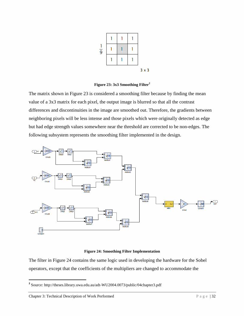
Figure 23: 3x3 Smoothing Filter2
The matrix shown in Figure 23 is considered a smoothing filter because by finding the mean
value of a 3x3 matrix for each pixel, the output image is blurred so that all the contrast
differences and discontinuities in the image are smoothed out. Therefore, the gradients between
neighboring pixels will be less intense and those pixels which were originally detected as edge
but had edge strength values somewhere near the threshold are corrected to be non-edges. The
following subsystem represents the smoothing filter implemented in the design.
Figure 24: Smoothing Filter Implementation
The filter in Figure 24 contains the same logic used in developing the hardware for the Sobel
operators, except that the coefficients of the multipliers are changed to accommodate the
2 Source: http://theses.library.uwa.edu.au/adt-WU2004.0073/public/04chapter3.pdf

Chapter 3: Technical Description of Work Performed P a g e | 33
smoothing filter. The adders and multipliers of the system make it very simple to understand and
use in future developments of the system without introducing timing errors. The only
accommodation that had to be made after introducing the smoothing filter was to add a delay to
the red, green and blue signals so that when they were added to the output of the edge detection
algorithm, the signals would still be synchronized.
The expansion of the system to include a smoothing filter in the design dramatically affected the
edge detection algorithm, despite the team‟s skepticism. The filter eliminated a significant
amount of noise in the edge detection output without sacrificing the quality of the edges detected.
The smoothing filter is a major advancement that provides a solution to edge detection in noisy
conditions, such as rain, where rain drops in the video stream should not be detected as edges.
Upon completion of the smoothing filter, the next major advancement in the system was the
introduction of skin detection. Skin detection is the process of identifying the pixels in an image
or video that have values similar to human skin. Design Team 3 has chosen to adopt a skin
detection algorithm (Peer) to alert of human presence within the camera‟s field of view. The
algorithm is a ruled based algorithm that detects skin in the RGB color space.
Figure 25: Skin Detection Logic
Finding the minimum and maximum values of the RGB signals is the first step towards
implementing the skin detection algorithm. Each signal is compared to one another using
relational blocks. The relational block outputs a 1 if the condition is true or a 0 if the condition is
false. A logical AND block is then used to determine what signal is the minimum. When a
signal outputs true for both relational blocks, the results of the logical AND will also be true.
The results of the logical AND block and are then multiplied with a constant. This constant is
used to identify which signal is the minimum.
Chapter 3: Technical Description of Work Performed P a g e | 34
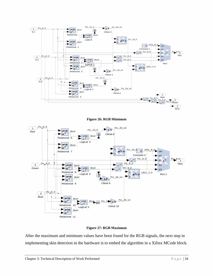
Figure 26: RGB Minimum
Figure 27: RGB Maximum
After the maximum and minimum values have been found for the RGB signals, the next step in
implementing skin detection in the hardware is to embed the algorithm in a Xilinx MCode block.
Min
4
Blue
3
Green
2
Red
1Relational 5
a
b
a<b
z-1
Relational 4
a
b
a<b
z-1
Relational 3
a
b
a<b
z-1
Relational 2
a
b
a<b
z-1
Relational 1
a
b
a<b
z-1
Relational
a
b
a<b
z-1
Mux
sel
d0
d1
d2
d3
z-1
Logical 2
and
z-0
Logical 1
and
z-0
Logical
and
z-0
z-3
z-3
z-4
z-4
z- 4
z- 3
cast
cast
cast
Constant 1
0
CMult 5
x 3
CMult 4
x 2
CMult 2
x 1
a
ba + bz-1
a
ba + bz-1
In3
3
In2
2
In 1
1
Fix _9_0
Fix _9_0
Fix _9_0
Bool
Bool
Bool
Bool
Bool
Bool
Bool
Fix_26_14
Fix _26_14
Fix_26_14
Fix_10_0
UFix _2_0
Fix _9_0
Fix_9_0
Fix_9_0
UFix_8_0
Bool
Fix_10_0
Bool
Fix_10_0
Fix_10_0
Fix _9_0Fix_9_0
Fix_9_0
Fix_9_0
Max
1
Relational 9
a
b
a>b
z-1
Relational 8
a
b
a>b
z-1
Relational 7
a
b
a>b
z-1
Relational 6
a
b
a>b
z-1
Relational 11
a
b
a>b
z-1
Relational 10
a
b
a>b
z-1
Mux 1
sel
d0
d1
d2
d3
z-1
Logical 5
and
z-0
Logical 4
and
z-0
Logical 3
and
z-0
z-3
z-3
z- 3
cast
cast
cast
Constant 2
0
CMult 9
x 2
CMult 8
x 1
CMult 10
x 3
a
ba + bz-1
a
ba + bz-1
Blue
3
Green
2
Red
1
Fix_9_0
Fix _9_0
Fix _9_0
Bool
Bool
Bool
BoolBool
Bool
BoolBool
Bool
Fix_26_14
Fix_26_14
Fix_26_14
Fix_10_0
UFix _2_0
Fix _9_0
Fix_9_0
Fix_9_0
UFix_8_0
Fix_10_0
Fix _10_0
Fix_10_0
Fix_9_0

Chapter 3: Technical Description of Work Performed P a g e | 35
The MCode block allows the use of basic MATLAB functions that then gets translated into
equivalent VHDL code when Xilinx System Generator is ran.
Figure 28: Xilinx System Generator's MCode Block
The MCode block used the design has the original red, green, and blue signals as inputs as well
as the minimum and maximum values found from Figures 26 and 27. It then performs the
algorithm outlined in Figure 29 and outputs the values of the original red, green, and blue signals
if skin is found or it sets all the signals to black if skin is not detected.
Figure 29: MCode Block Code
The output from the MCode block can is then displayed on the monitor. Design Team 3 also
chose to build in the option to combine output of the skin detection algorithm with the results of
the Sobel edge detection. When these two signals are multiplied together, only the edges of
pixels that were found to be skin will be visible.

Chapter 3: Technical Description of Work Performed P a g e | 36
The skin detection algorithm was first tested as an expansion to the still image edge detection
system because of the simpler approach it allows for troubleshooting. Once implementation in
that system was successful, the same system was adapted to the video detection system in the
same way the edge detection system was adapted. The only changes that were required to
accommodate the additional system were additional delays after the skin detection algorithm
because it acts in parallel with the edge detection, and all outputs must be synchronized.
The skin detection algorithm completes the major components of the entire detection system, and
the remaining efforts that were made toward the edge and skin detection system were to use
several multiplexers (MUXs) as switches so that the user can control what systems are activated
in the video output. The controlling of these MUXs is implemented using register blocks.
Registers are a key component in the design enabling the ability to turn features on and off
through software. A single 8-bit register is used to control the following features of the hardware
design: video overlay, Sobel X, Sobel Y, combined Sobel, smoothing filter, skin detection, and
skin detection combined with edge detection. Each feature is assigned a single bit within this
register. The bit field layout is show below in Figure 30.
Figure 30: Bit Field Layout
The above features are on when the value of the assigned bit is set to 1. In order to assure that
each feature gets their corresponding bit from the register, a slice block is used. The slice block
gives the ability to remove a sequence of bits from the input data and outputs the new value. By
combining the output of the register with slice blocks Design Team 3 was able to control

Chapter 3: Technical Description of Work Performed P a g e | 37
multiple features with a single 8-bit value, which in turn uses less memory and simplifies the
ability to control more than one feature at a time as shown below in Figure 31.
Figure 31: Combination of Register and Slice Blocks
A second 8-bit register is used the hold the value of the threshold for the Sobel edge detection
algorithm. This register is initially set to a default value of 70. Through software, the user has
the ability to increase or decrease this value.
The final piece of hardware used in combination with the registers and slices to control the
features of the design is a multiplexer or mux. A multiplexer makes it possible for several inputs
to share one output. The select port on the multiplexer is used to turn on the input signal that
will be sent to the output. Using multiplexers in the design is a big savings on cost when it
comes to hardware resources being used. For example, Figure 32 shows a multiplexer that is
capable of having eight different inputs that are all controlled through the select port. All of the
inputs can share a single output resource, which is far more efficient than having eight of the
same types of output.

Chapter 3: Technical Description of Work Performed P a g e | 38
Figure 32: MUX (Multiplexer) with 8 Inputs
Using the MUXs and register blocks provides a user-friendly system of displaying the different
subsystems within the detection system. This concludes the development of the hardware for the
edge detection and person detection algorithms, and the testing results for all aspects of this
system can be seen in Chapter 4.
3.2 Software Design
After hardware design is complete, the final piece of the embedded system is developing
software to direct the operation of the FPGA and its connected peripherals. The development kit
used in this project is equipped with a Microblaze 32-bit processor that can be instructed using
the C programming language. Users interact with the FPGA through a terminal program such as
PuTTY, to control the various features that have been developed in hardware using Xilinx
System Generator. Modifications were made to the code included with the Camera Frame
Buffer Demo provided by Xilinx to fit the needs of Design Team 3.
3.2.1 Main Menu
The main menu is the first thing that the user will see when the program is started. There is only
one option available for selection at this menu and that is to enter the edge detection menu by
typing an „e‟ into the terminal window. The following code in Figure 33 produces the output
shown in Figure 34.

Chapter 3: Technical Description of Work Performed P a g e | 39
Figure 33: Main Menu Code
Figure 34: Main Menu Display
3.2.2 Edge Detection Menu
The edge detection menu gives the user control of the algorithms and hardware designs that have
been created using Xilinx System Generator. Selecting an option in this menu will change the
value of the registers discussed in Section 3.1.

Chapter 3: Technical Description of Work Performed P a g e | 40
Figure 35: Edge Detection Menu
The following code produces the edge detection menu:
Figure 36: Edge Detection Menu Code
XOR along with AND logic are used to determine what the value in the status register should be.
When a feature is selected, using XOR logic with the bit assigned to that feature will turn it on
(set value to 1) when it is currently off and also turn it off (set value to 0) when it is currently on.
AND logic is used to check the current value of the register without affecting the status of the

Chapter 3: Technical Description of Work Performed P a g e | 41
feature. Certain menu options, such as the Combined Sobel, require both the Sobel X and the
Sobel Y to be on. However, if a logical XOR were used without checking the current value of
the bit, it would give the undesired effect of setting the bit to 0 when truly a 1 is desire. The truth
tables for the logic used are shown below in Figure 37 and Figure 38.
Figure 37: XOR Logic (shown on left) and AND Logic (shown on right)3
A series of case statements are used to combine the user input with the desired output. Below is
an example of how the software reads the value from the register, performs logic on it, and
rewrites the new value to the register.
Figure 38: Software Reads, Performs Logic, and Rewrites Register Value
3 source: www.eetimes.com

Chapter 3: Technical Description of Work Performed P a g e | 42
The software will also alert the user whether they turned the feature on or off.
Figure 39: Overlay Status
3.2.3 Object Detection Implementation
At the start of the project, the team planned on implementing object detection through higher
level programming languages such as C++ and OpenCV (Open Source Computer Vision)
imported into the board. Significant time was spent researching and finding potential open
source programming implementations. Some researched methods did object detection and even
object identification through the use of large database classifiers instead of edge detection.
Implementing a very complex algorithm onto the Xilinx Spartan 3A FPGA Development Board
optimized for high level of mathematic operations became the initial plan.
Many solutions were researched for implementing high level code onto the board. One solution
had C code converted to VHDL but it was found that companies often pay thousands of dollars
for this time intensive task to be done. Another involved using Matlab to call an external
database of images for comparison of if shapes in the image were objects. Extensive research
was also done in Xilinx‟s Software Development Kit (SDK) for use of the C++ code that the
MicroBlaze processor uses on the board for instructions. The hope was that C++ code ran there
could be used for object detection but the MicroBlaze is not optimized for intensive computation
instructions.
It was not until the team fully realized the limitations and purpose of the Xilinx Spartan-3A
FPGA that the team found a way to implement object detection. The board‟s specialty is math

Chapter 3: Technical Description of Work Performed P a g e | 43
intensive computations. With knowledge also gained from edge detection, the team researched
Matlab code and the possibility of breaking down a Matlab programming file down into Xilinx
Blocks using Xilinx System Generator in Simulink. More reason to implement object detection
came with knowledge of the “MCode” block in Xilinx System Generator.
The MCode block allows a Matlab file to be implemented into Xilinx blocks. As long as inputs
and outputs are designated in the Matlab file, those inputs and outputs are displayed in the
MCode block and can be connected to any other Xilinx blocks. Figure 40 displays how Matlab
code is integrated into Xilinx blocks. The problem is that the MCode block supports a limited
range of Matlab functions and data types.
Figure 40: Example of MCode Implementation into Xilinx Blocks in Simulink
3.2.4 Software Design
One on the most challenging tasks in Computer Vision is feature extraction in images. Usually
objects of interest may come in different sizes and shapes, not pre-defined in an arbitrary object
detection program. A solution to this problem is to provide an algorithm than can be used to find

Chapter 3: Technical Description of Work Performed P a g e | 44
any shape within an image then classify the objects accordingly to parameters needed to describe
the shapes. A commonly used technique to achieve this is the Hough Transform. Invented by
Richard Duda and Peter Hart in 1992, the HT was originally meant to detect arbitrary shapes of
for different objects. The Hough Transform was later extended to only identify circular objects in
low-contrast noisy images, often referred to as Circular Hough Transform.
Figure 41: Hough Transform Excerpt4
4 The following applet demonstrates the circular Hough Transform and was created by Mark A.
Schulze http://www.markschulze.net/.

Chapter 3: Technical Description of Work Performed P a g e | 45
This method highly depends on converting gray-scale images to binary images using edge
detection techniques such as Sobel or Canny. The goal of this technique is to find irregular
instances of objects within a pre-defined set of shapes by a voting procedure. Using information
about the edges already available from our edge detection algorithm using Xilinx‟s system
generator blocks makes the computational requirements less complex. Unlike the linear HT, the
CHT relies on equations for circles. The equation of the a circle is;
r² = (x – a)² + (y – b)² (1)
Here a and b represent the coordinates for the center, and r is the radius of the circle.
The parametric representation of this circle is;
x = a + r*cos(θ)
y = b + r*sin(θ) (2)
For simplicity, most CHT programs set the radius to a constant value or provides the user with an
option to set a range (maximum and minimum) prior to running the application.
Figure 42: Computation of Circular Hough Transform

Chapter 3: Technical Description of Work Performed P a g e | 46
The program then uses information about detected edges from the edge detection algorithm, that
is, the coordinate (x and y) of each edge point and creates a 3 dimensional array with the first
two dimensions representing the coordinates of the circle and the last specifying the radii.
For each edge point, a circle is drawn with that point as origin and radius r. The values in the
accumulator are increased every time a circle is drawn with the desired radii over every edge
point. The accumulator, which kept counts of how many circles pass through coordinates of each
edge point, proceeds to a vote to find the highest count.
3.2.5 Software Implementation
Due to the nature of the system generator being created in a Matlab/Simulink, we decided that
writing our code in Matlab would result in less complexity in communicating with the FPGA
board. Given the time constraint, we decided that researching an existing Circular Hough
transform algorithm using Matlab then implementing it using Xilinx‟s system generator block
would be more time efficient.
On page XX is a program entirely written in Matlab for detecting circular shapes patterns within
an input image. We choose this program because it does not make use of circular/trigonometric
functions for determining the candidate circles. Instead, several matrices are defined to store
information about edge point and the distance from that point to every circle center already
computed. Below is a snippet that illustrates this concept in much more details.
Figure 44: Input Image After Edge Detection Figure 43: Image After Voting

Chapter 3: Technical Description of Work Performed P a g e | 47
Figure 45: Snippet of Circular Hough Transform Calculation
Matlab code result on images with coins.
Figure 46: Circular Hough Transform Output
Unfortunately, system generator does not support matrix operations on the FPGA. Also, only
subsets of Matlab operations were available for use. We decided that treating each column in a
matrix as a vector then hard coding some of the complex Matlab operations would considerably
decrease FPGA computational demands thus reducing the amount of complexity. MCode blocks
were considered for creating and looping and indexing the vectors.
Since this project spans multiple semesters and due to limited amount of time available needed to
debug and run images through our program, we decided that the current model was a good

Chapter 3: Technical Description of Work Performed P a g e | 48
stopping point for this semester and a good starting point for next semester‟s student team. The
entirety of the Circular Hough Transform code can be found in Appendix 3.3.

Chapter 4: Test Data with Proof of Functional Design P a g e | 49
Chapter 4: Test Data with Proof of Functional Design
Design Team 3‟s project was subdivided into two areas: edge detection and object detection. The
main goal of the team was for a successful edge detection algorithm running smoothly on live
video with a higher goal of implementing some form of object detection.
4.1 Testing Edge Detection
Using this setup, the algorithm was ran and tweaked according to more ideal outputs as detailed
in Chapter 3. Added functionality was also added, with button toggles controlling the original
background image, Sobel X, Sobel Y, a smoothing filter, threshold down, threshold up, reset
threshold, human detection, and human detection with edge detection.
The Sobel X and Y outputs measure the individual outputs of the Sobel filters. These outputs are
then summed into a single complete Sobel filter. This was included to showcase the inner
workings of the Sobel edge detection algorithm. The complete Sobel edge detection output is
further improved by a smoothing filter. This works by scanning every pixel individually, finding
the intensity value for that pixel and the surrounding pixel of a 3x3 matrix, and then averaging
that pixel with the surrounding pixels. This extracts noise while filling in lines and curves
important to the output. Manual threshold adjusting was also added to the interface. Although the
ideal threshold for the algorithm was found to be 70, this can be manually adjusted depending on
the situation for display purposes. This value can also be easily adapted back to a threshold of 70
at any time by a push of the button.
Overall, the edge detection part of the project is very successful. It is impressive at detecting
edges and much of its success is because of its adaptability. The thresholds can be adjusted
depending on the situation and the variety of outputs provides a fuller picture to the inner
workings of the algorithm and allows simultaneous comparisons. It is fully functional, operates
via video in real time, and is easily accessible for future design implementations. Team 3
believes that edge detection meets all of the design specifications described in Chapter 2 and is
complete.

Chapter 4: Test Data with Proof of Functional Design P a g e | 50
Figure 47: Standard Unmodified Video
Figure 48: Sobel X

Chapter 4: Test Data with Proof of Functional Design P a g e | 51
Figure 49: Sobel Y
Figure 50: Combination of Sobel X and Sobel Y into Full Sobel Algorithm

Chapter 4: Test Data with Proof of Functional Design P a g e | 52
Figure 51: Smoothing Filter
Figure 52: Threshold at 20- Set too Low

Chapter 4: Test Data with Proof of Functional Design P a g e | 53
Figure 53: Threshold at 220- Set too High
Figure 54: Full Edge Detection Over Source Video Feed

Chapter 4: Test Data with Proof of Functional Design P a g e | 54
4.2 Testing Human Detection
Human detection was also implemented, using skin to highlight humans in the video feed. It
operates simultaneous to edge detection without any noticeable timing delays. It can also be
utilized to output its display in unison with some of the edge detection features. Design Team 3‟s
implementation has two specified outputs: the output of human detection and such output in a
logical AND with edge detection. The former passes through what it finds to be skin while
blocking out everything else. The logical AND with human detection and edge detection
highlights the edges of what it finds to be human skin which is useful for potentially alerting the
driver of humans in the camera‟s view. Such output has a bright red color for this purpose.
Overall, human detection is an impressive addition to edge detection. It is very good at correctly
identifying human skin on the image. There is room for improvement, however, as it has many
false positives. The false positives occur because it is based on the wide range of colors of skin.
A key future improvement could be tweaking the algorithm to properly negate these false
positives. Human detection has many useful applications for preventing harm to pedestrians in
automotive applications and the algorithm is a strong step towards prevention.

Chapter 4: Test Data with Proof of Functional Design P a g e | 55
Figure 55: Human Detection
Figure 56: Edge Detection and Human Detection

Chapter 4: Test Data with Proof of Functional Design P a g e | 56
4.3 Testing Object Detection
Object detection was unfortunately a successful failure. Object detection on the Xilinx Spartan
3A-3400 Board is a difficult task and object detection is the topic of many professors‟ research
labs in universities around the globe. Training a computer to see like a human is a difficult task,
one that requires analysis of how humans determine objects in a logical way. The thought
process must then fit the confines of a programming language.
The primary problem is that the board itself only supports low level Matlab code in addition to a
primarily math driven graphical based programming interface. Many object detection algorithms
are based on 3D Matrices which can be compared to the pixels around it in a 2D plane. Low-
level code is supported via an “MCode” Block within the interface which can run a limited
amount of Matlab functions. Unfortunately, the MCode Block does not support NxN matrices
and only supports 1xN vectors. This creates the core issue as the key component of the Hough
algorithm is a 3D Matrix. The MCode block‟s support of only 1D matrices adds an
overwhelming amount of complexity to find these computations. As detailed in Chapter 3, more
tweaks to the code in order to accommodate System Generator‟s MCode Block are needed in
order for it to output the correct identification of circles.
The MCode Block‟s limitation led to a complete overhaul of open source Circular Hough
Transform code in order to accommodate its limited functionality. The software intensive nature
on a mostly Electrical Engineering team proved to be a mismatch. An example of the complexity
in the transformation is displayed in Figure57. A more clear initial understanding of how to
implement object detection would have allowed the additional time required to complete the
object detection of circles in Team 3‟s project.

Chapter 4: Test Data with Proof of Functional Design P a g e | 57
Figure 57: Conversion from Higher Level Matlab Syntax to Equivalent Lower Level Syntax
This project is designed for multiple semesters and this work is only the beginning. The hope is
for future teams to contribute more image processing tools onto Design Team 3‟s project. Future
implementations of object detection, object identification, distance detection, could only be the
future of Xilinx‟s Michigan State University collaboration.

Chapter 5: Final Cost, Schedule, Summary and Conclusion P a g e | 58
Chapter 5: Final Cost, Schedule, Summary and Conclusion
Design Team 3 has laid impressive groundwork for object detection implementation and further
image processing algorithms. They structured their algorithms and designed the system in a
manner that could be easily expanded upon. The team successfully designed edge detection, skin
detection, and human detection; all of which can be placed over the original video feed and
displayed on the monitor. Both the edge detection and skin detection features behave as one
would expect but the human detection combines both of these features for a third output option.
The team has made significant headway in circle detection but was unable to debug the code in
time for the design day demonstration.
One major finding of Design Team 3 was the necessity of Xilinx‟s System Generator blocks.
Implementation of algorithms within a 15 week period could only be achieved by using the
System Generator blocks; additional implementation methods would have required a
significantly longer amount of time. Before the team learned the inevitability of using System
Generator blocks, they examined using OpenCV methods for object detection. OpenCV allowed
the flexibility of training a classifier to detect specific objects through the use of a method known
as Haar Training. This solution would have been very appropriate if object detection could have
been implemented using a computer; the FPGA‟s coding limitation made this solution unfeasible
for the project. The primitive coding capability of System Generator was the biggest handicap
during implementation. Very few Matlab commands are available within the MCode block and
the remaining system must be designed utilizing very basic graphical blocks. All of the
implemented features utilize a morphological smoothing block which assists further image
processing functions. By blurring the discontinuities and edges into surrounding pixels, the
smoothing block removes image noise therefore increasing final output accuracy.
The design team has several recommendations for future teams that inherit this project regarding
object detection. First, the team must familiarize themselves with Xilinx‟s tools and specifically
with the capabilities of System Generator. By understanding the language level available within
System Generator, an algorithm can be more easily created. Second, completion of circle
detection using System Generator blocks must be an initial goal. This will allow the team to
become better acquainted with Xilinx‟s tools and design platform as well as create the first step

Chapter 5: Final Cost, Schedule, Summary and Conclusion P a g e | 59
in object detection. Lastly, detection of other shapes and combination of shapes would prove
useful; by combining shapes, more complex objects could be detected.
The majority of the materials necessary to complete this project were provided by either Xilinx
or Michigan State University to the team. The Xtreme DSP Video Starter kit for an estimated
$2,695.00 market value, monitor and cables for $100, ISE Design Suite for $99.99, and
Matlab/Simulink package for $99.00 were provided; a USB-A to serial cable was purchased for
$40.98 by the team. Thus bringing the total cost to $3,034.97 of which only $40.98 was the cost
to the design team.

Appendix 1: Technical Roles, Responsibilities, and Work Accomplished P a g e | 60
Appendix 1: Technical Roles, Responsibilities, and Work Accomplished
This appendix describes the individual technical contributions of each ECE480 Design Team 3
member.
A1.1 Fatoumata Dembele - Webmaster
Fatoumata Dembele‟s technical portion of the project consisted
of gathering information about different object detection
techniques currently in use and freely available that can be
implemented on the FPGA board provided by Xilinx. Two of the
main methods used in object detection are OpenCV, a library of
programming function for real time computer vision, and the
Matlab Image Processing Toolbox.
Fatoumata‟s first attempt was to import the OpenCV library into the Xilinx EDK environment in
order to run an image processing application. The initial idea was to run C/C++ applications on
the MicroBlaze processor using Xilinx‟s SDK. Since all image processing algorithms involve
operations on matrices, a software implementation rather than hardware, would result in less
complexity for debugging. After some intensive research on OpenCV, she realized that this
approach had several constraints, notably dealing with converting floating points to fixed points
for FPGA simulation.
The second attempt consisted of taking advantage of a web based image annotation tool provided
by MIT called LabelME for object recognition. The motivation was to use a Matlab program
(provided by the MIT Computer Science and Artificial Intelligence Laboratory) called Simple
Object Detector Using Boosting on each frame of our input video for detecting pre-defined
objects. This approach would require a considerable amount of time for processing videos in real
time and would not have been fully implemented by our final design due date.
Fatoumata‟s last and final approaches consisted of using our working edge detection algorithm
implemented in System Generator Blocks and performing some mathematical operations using a
feature extraction method. A popular and rather simple method of detecting particular shapes

Appendix 1: Technical Roles, Responsibilities, and Work Accomplished P a g e | 61
within an image is the Hough Transform. This method was later extended to detect circular
shapes, called Circular Hough Transform (CHT). The idea is to use results from the Sobel edge
detector and perform operations for circular object recognition. This goal appeared achievable
within a reasonable timeframe.
Fatoumata, Pascha, and Emmett worked together on implementing the CHT Matlab code using
Xilinx‟s System Generator blocks. Due to timing constraints, they could not debug the program
accordingly for the desired results.
A1.2 Chad Eckles – Lab Coordinator
Initially Chad Eckles was responsible for researching edge
detection. He extensively researched the different edge detection
methods and how each one operates. While researching edge
detection he was simultaneously researching the capabilities of
Simulink and trying to decide which edge detection methods
were best suited for implementation in Simulink. Chad was able
to narrow the choices down to two edge detection methods. The group along with Chad was not
able to come to a decision on which method to use, so Chad created a solution selection matrix to
help make a decision. Based on the matrix the group agreed that Sobel edge detection was the
best selection.
Based on the extensive research done on edge detection and Simulink, he along with Tom
Ganley and Jeff Olsen, primarily worked on developing an algorithm for edge detection. He first
started off by creating an algorithm in Simulink without the use of Xilinx blocks in order to gain
a better understanding of how a proper algorithm should flow. This approach also helped the
team to understand how the values of thresholds affect the images and how the normal values
should be set. He was then able to transfer the properties of thresholding and flow into the design
of the edge detection algorithm using Xilinx blocks. The algorithm was developed by first
creating an R-G-B (Red, Green, and Blue) to Grayscale color conversion, followed by a Sobel
edge detection algorithm. He was able to help design and test some of the R-G-B to grayscale
conversions and edge detection algorithms on still images. Once still image algorithms worked
he aided in developing the live video edge detection algorithm using Xilinx blocks. After the

Appendix 1: Technical Roles, Responsibilities, and Work Accomplished P a g e | 62
algorithm was developed, Chad, alongside Jeff Olsen and Tom Ganley, spent countless hours
trying to debug the algorithm.
Once the algorithm was almost working properly, Chad switched over to the object detection
team. Since he had an extensive amount of work with Simulink, Xilinx, and edge detection, he
was able to transfer his knowledge to helping the object detection team. Chad was able to help
with some of the lines in the Matlab code to rewrite them for use in Xilinx blocks.
A1.3 Pascha Grant – Documentation Preparation
Pascha Grant began the semester with her primary role in
researching edge detection and object detection. Her acquired
knowledge of the four edge detection methods available in
Matlab allowed the team to compare and contrast the features of
each. Once the edge detection method was determined, the
process of implementing the algorithm was passed on to Tom
and Jeff, her concentration shifted to object detection. She focused on determining object
detections methods utilizing top-down recognition with her main focus on implementing object
detection using a classifier within Matlab. By providing Matlab with both positive and negative
images of the object to be detected, Haar Training can be used to teach a classifier to recognize
the object within a new image. She spent a significant amount of time learning how to train a
classifier from thousands of sample images, when the design team discovered that a classifier
could not be implemented onto the FPGA.
Her primary role then changed direction towards bottom-up object classification. After
researching the subject, it was determined that in order to implement object detection, basic
shapes must first be able to be recognized. Emmett, Fatoumata, and Pascha began looking into
the Circular Hough Transform. The main problem with implementing the Circular Hough
Transform was the need for simplistic code. The team knew that they did not have enough time
to create code from scratch, thus the focus was to convert an existing code into Xilinx‟s System
Generator blocks. System Generator is very limited as far as programming languages are
concerned therefore only basic commands could be utilized.

Appendix 1: Technical Roles, Responsibilities, and Work Accomplished P a g e | 63
When a simplistic Matlab version of the Circular Hough Transform was found, Pascha took the
lead role of converting it into lower-level building blocks of code. She placed all of her focus
into creating an even more simplistic version of the transform and faced many challenges. One of
the biggest challenges while converting the code was the use of matrices. The original code used
three-dimensional matrices but an FPGA can only use horizontal vectors. This meant that every
time a matrix was used, a nest of loops had to be created to convert the matrix into a vector with
a considerable number of elements. Not only did matrices prove to be a challenge, but higher-
level syntax such as „slice‟ and „find‟ within Matlab had to be converted as well.
Although the conversion had to consist of low level commands, MCode blocks were
implemented to aid in the computation. Emmett familiarized himself extensively with the
MCode block‟s capabilities so that Pascha could focus on writing the code and muster Emmett‟s
know-how as needed. The code was completely converted into basic commands that could very
easily be built using System Generator; however she was left without ample time for debugging.
The final code is able to compile but may be a week or two away from being debugged in order
to display the proper output. The group that inherits this project should be able to implement
circle detection within a week of learning the applications.
A1.4 Tom Ganley - Rover
Tom‟s initial technical role this semester was to aid in the
research of edge detection and object detection algorithms that
could be implemented in Matlab and Simulink. He studied demo
applications of both edge and object detection to understand
what types of systems could be implemented using simple
mathematics and which could not. Through the use of simple
Simulink blocks, Tom gained valuable experience in understanding the Simulink design
environment that proved beneficial to the team‟s forward progress using Xilinx‟s System
Generator software.
At the point in time that the team understood that all developments of edge and object detection
would need to be implemented using Xilinx‟s System Generator blocks; he was assigned to work
with Chad Eckles and Jeff Olsen to develop an edge detection algorithm using these blocks
Appendix 1: Technical Roles, Responsibilities, and Work Accomplished P a g e | 64
based on knowledge gained during the research stages. Very quickly, Tom was responsible for
the team‟s first implementation of grayscale conversion using only Xilinx blocks on a still
image. Shortly afterwards, he also implemented the first low-level edge detection algorithm with
the Xilinx blocks. Though the algorithm was performed on a still image and was tested using
simulation, this quick advancement proved to be essential to the team‟s success as only minor
changes were made to this subsystem throughout the semester to accommodate for video edge
detection.
Upon completion of edge detection on a still image, Tom joined Jeff and Chad in troubleshooting
the system for video edge detection. The three of them spent many hours making minor changes
to the system that made logical sense to try implementing successful edge detection. One
contribution that Tom made during the troubleshooting stages was the discovery that a 3x3 Sobel
operator would reduce the majority of the noise being seen in the system, as opposed to a 5x5
operator. It was not until Jeff introduced a new form of implementing the Sobel operators that
the team was able to implement a very accurate and noise-free system.
Once the team had successfully implemented edge detection on the video stream from the
camera, Tom was responsible for introducing a smoothing filter into the hardware. Using Jeff‟s
new structure of Sobel operators, Tom developed a matrix operator that smoothed all edges and
discontinuities in the source image so that the edge detection algorithm was more successful and
accurate with a significant reduction in the amount of noisy pixels in the output.
Finally, Tom was responsible for assisting Jeff in the implementation of skin detection on the
video stream. Tom and Jeff each found a very simple implementation of skin detection, and both
of them began attempting to achieve success in their respective discoveries. Pressed on time, Jeff
was able to successfully implement skin detection first, so Tom joined him in expanding the
detection system to include the skin detection. Tom aided by testing Jeff‟s system on a still
image by expanding the still image edge detection system he had implemented earlier in the
semester. Tom‟s final contribution to the team was suggesting that by multiplying the edge
detected signal in the system with the skin detection signal, only those edges that were also
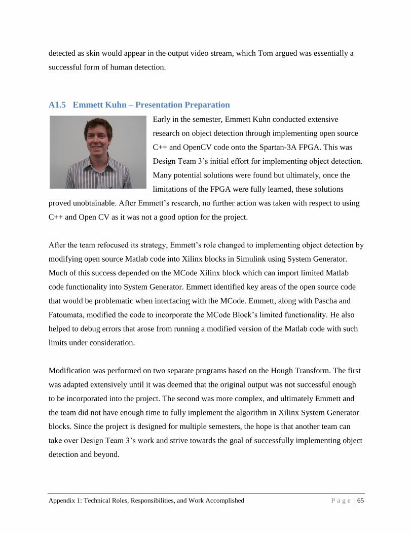
Appendix 1: Technical Roles, Responsibilities, and Work Accomplished P a g e | 65
detected as skin would appear in the output video stream, which Tom argued was essentially a
successful form of human detection.
A1.5 Emmett Kuhn – Presentation Preparation
Early in the semester, Emmett Kuhn conducted extensive
research on object detection through implementing open source
C++ and OpenCV code onto the Spartan-3A FPGA. This was
Design Team 3‟s initial effort for implementing object detection.
Many potential solutions were found but ultimately, once the
limitations of the FPGA were fully learned, these solutions
proved unobtainable. After Emmett‟s research, no further action was taken with respect to using
C++ and Open CV as it was not a good option for the project.
After the team refocused its strategy, Emmett‟s role changed to implementing object detection by
modifying open source Matlab code into Xilinx blocks in Simulink using System Generator.
Much of this success depended on the MCode Xilinx block which can import limited Matlab
code functionality into System Generator. Emmett identified key areas of the open source code
that would be problematic when interfacing with the MCode. Emmett, along with Pascha and
Fatoumata, modified the code to incorporate the MCode Block‟s limited functionality. He also
helped to debug errors that arose from running a modified version of the Matlab code with such
limits under consideration.
Modification was performed on two separate programs based on the Hough Transform. The first
was adapted extensively until it was deemed that the original output was not successful enough
to be incorporated into the project. The second was more complex, and ultimately Emmett and
the team did not have enough time to fully implement the algorithm in Xilinx System Generator
blocks. Since the project is designed for multiple semesters, the hope is that another team can
take over Design Team 3‟s work and strive towards the goal of successfully implementing object
detection and beyond.

Appendix 1: Technical Roles, Responsibilities, and Work Accomplished P a g e | 66
A1.6 Jeff Olsen - Manager
Xilinx provided Design Team 3 with a Spartan 3A-3400 Xtreme
DSP Development Kit to use as the platform for the assigned
project. Jeff Olsen was initially responsible, along with Chad
Eckles, to learn the proper configuration of the development kit
so the team could see the provided demos of the FGPA in action.
Early in the semester Jeff realized that key components of the
system needed to complete the project still had to be acquired by the team. Without the team‟s
acquisition of the missing pieces, they would have had no way to interact with the camera or
program the FPGA.
After all of the pieces to the development kit were in place and the team was still unsure of the
best direction for the project, the one thing that was sure was the fact that Design Team 3 would
need to figure out how to integrate with the video stream entering the FPGA from the camera.
Jeff Olsen was then responsible for learning the process of taking the provided Xilinx Camera
Frame Buffer Demo from the MATLAB/Simulink environment to an embedded system on the
Spartan 3A development board. This involved learning the process of generating a pcore using
Xilinx System Generator, generating a bitstream and building software applications in Xilinx
Platform Studio, downloading the bitstream to the FPGA, and running the program through
Xilinx Microprocessor Debugger. This was a big step for the design team, as it was now
understood how the algorithms that were developed would be implemented into the camera
stream.
Jeff then joined a team with Tom Ganley and Chad Eckles. Together they were responsible for
translating the Sobel edge detection algorithm into a low level design using the Xilinx Blockset
in the Simulink environment and implementing it into the camera stream. The team‟s initial
attempts at implementing the algorithm stemmed from a still image edge detection model that
Tom Ganley was responsible for introducing to the team. This model proved to be successful at
detecting edges in still images, but when integrated with the video stream the model introduced
significant delay that was unacceptable for real time image processing. Although this model was
seen as unsuccessful in performance, it served as the spark the team needed to complete edge

Appendix 1: Technical Roles, Responsibilities, and Work Accomplished P a g e | 67
detection in a video stream. The edge detection team‟s original model used a 5-line buffer
combined with a 5x5 convolution mask. Jeff was responsible for introducing the team to a 3x3
model that successfully detected edges in a live video stream and became the model
implemented in the final design.
Jeff then proposed the idea of using registers and C code to provide a user interface that allowed
the features developed by the team to be controlled by input through a terminal program. Jeff
was responsible for developing the logic used to control the values in the registers and also
writing the C code that would implement the logic.
The final technical role that Jeff was responsible for was implementing a skin detection
algorithm with the assistance of Tom Ganley. After the team decided to use skin detection as a
way to identify and alert human presence within the camera frame, Jeff was responsible for
introducing the team to an algorithm that had the capabilities of operating on a live video stream
in the RGB color space. Jeff and Tom then performed testing on the algorithm to assure that the
algorithm would successfully detect a diverse range of skin. After testing, Jeff was responsible
for building a model using the Xilinx Blockset and implementing it into the final design.

Appendix 2: Literature and Website References P a g e | 68
Appendix 2: Literature and Website References
“ An Introduction to Edge Detection: The Sobel Edge Detector”. Generation 5. 2002. September
17, 2010. <http://www.generation5.org/content/2002/im01.asphttp:// >.
“Adapting the Sobel Edge Detector and Canny Edge Extractor for iPhone 3GS Architecture”.
IWSSIP. 2010. September 17, 2010.
<www.ic.uff.bf/iwssip2010/proceedings/nav/papers/paper_161.pdf>.
“Canny Edge Detection”. Ruye Wang. 2004. October 17, 2010.
<http://fourier.eng.hmc.edu/e161/lectures/canny/node1.html>.
“Coordinate Geometry: circles, ellipses”. A-Level Maths Tutor. 07/12/2010. <http://www.a-
levelmathstutor.com/circles-ellipses.php>.
“Edge Detection”. CNX. 2010. September 17, 2010. <http://
www.cnx.org/content/m24423/latest/>.
“Fujitsu Ten Press Release”. Fujitsu Ten. 2010. September 22, 2010. <http://www.fujitsu-
ten.co.jp/english/release/2010/04/20100420_e.html>.
“Gentex Mirror with Rear Camera Display”. Mechanics Warehouse. 2005-2008. September 22,
2010. <http://www.mechanics-warehouse.com/mito-autodim-camera.htm>.
“How to build a cascade of boosted classifiers based on Haar-like features”. KYUtech.Florian
Adolf. 2003. October 17, 2010.
<http://lab.cntl.kyutech.ac.jp/~kobalab/nishida/opencv/OpenCV_ObjectDetection_HowTo.pdf>.
“Human Skin Colour Clustering for Face Detection”. Jure Kovaˇc, Peter Peer, and Franc Solina
University of Ljubljana:Faculty of Computer and Information Science. Trˇzaˇska 25, SI-1000
Ljubljana, Slovenia <E-mail: [email protected], [email protected], [email protected]
lj.si>.
“Sanyo Automotive Equipment”. Sanyo North America Corporation. 2010. September 22, 2010.
<http://us.sanyo.com/Automotive-Equipment>.
“Vehicle Vision Sensing”. John Day‟s Automotive Electronics News. 2010. JHDay
Communications powered by WordPress. September 17, 2010.
<http://johndayautomotivelectronics.com/?p=60>.
“Xilinx Automotive Optical Flow Solution Addresses Image Processing Requirements of
Advanced Driver Assistance Systems”. EDACafe. 2010. September 22, 2010.
<http://www10.edacafe.com/nbc/articles/view_article.php?articleid=615707&interstitial_display
ed=Yes>.
Epitropou, Victor. “Enhanced (Circular) Hough Transform”. DUTh Circle Detection. 2005-2006.
11/15/2010. <http://www.papamarkos.gr/uploaded-
files/Papaparkos/demos/GHT/Help/EHT.htm>.

Appendix 2: Literature and Website References P a g e | 69
Gregg A. Motter. “Function Definition: A Powerful Problem or Opportunity Analysis
Technique”. 2006 & 2008.
Just Kjeldgaard Pedersen, Simon. “Circular Hough Transform.” Aalborg University, Vision,
Graphics, and Interactive Systems. November 2007. 11/15/2010.
<http://www.cvmt.dk/education/teaching/e07/MED3/IP/Simon_Pedersen_CircularHoughTransfo
rm.pdf >.
Mona K. Garvin. “Segmentation: Edge-based segmentation”. Digital Image Processing. 07/12/2010.<http://www.icaen.uiowa.edu/~dip/LECTURE/Segmentation2.html >.

Appendix 3: Referenced Figures P a g e | 70
Appendix 3: Referenced Figures
A3.1 Initial Gantt Chart
Figure 58: Initial Gantt Chart, 1 of 2

Appendix 3: Referenced Figures P a g e | 71
Figure 59: Initial Gantt Chart, 2 of 2
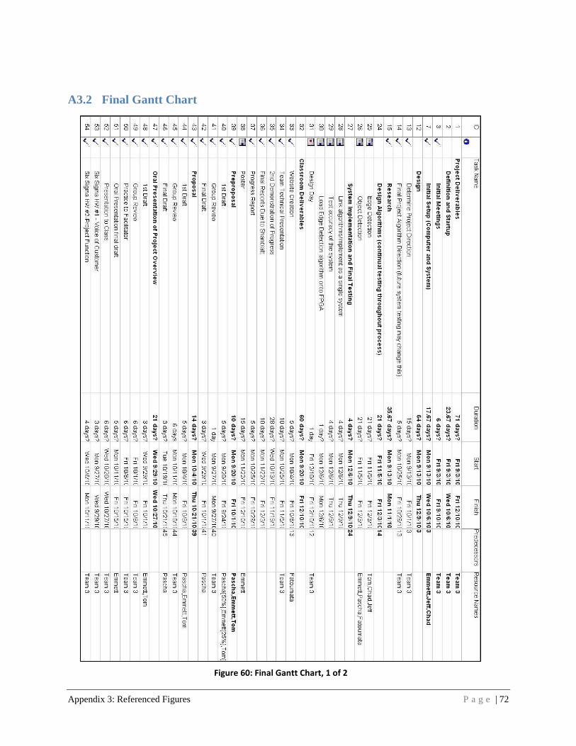
Appendix 3: Referenced Figures P a g e | 72
A3.2 Final Gantt Chart
Figure 60: Final Gantt Chart, 1 of 2

Appendix 3: Referenced Figures P a g e | 73
Figure 61: Final Gantt Chart, 2 of 2

Appendix 3: Referenced Figures P a g e | 74
A3.3 Circular Hough Transform (Open Source Code Freely Available)
function circles = houghcircles(im, minR, maxR, thresh, delta) % Copyright (c), Yuan-Liang Tang % Associate Professor % Department of Information Management % Chaoyang University of Technology % Taichung, Taiwan % http://www.cyut.edu.tw/~yltang % % Permission is hereby granted, free of charge, to any person obtaining % a copy of this Software without restriction, subject to the following % conditions: % The above copyright notice and this permission notice should be included % in all copies or substantial portions of the Software. % % The Software is provided "as is," without warranty of any kind. % % Created: May 2, 2007 % Last modified: Jan. 8, 2009 % % Check input arguments if nargin==3 thresh = 0.33; % One third of the perimeter delta = 12; % Each element in (x y r) may deviate approx. 4 pixels elseif nargin==4 delta = 12; end if minR<0 || maxR<0 || minR>maxR || thresh<0 || thresh>1 || delta<0 disp('Input conditions: 0<minR, 0<maxR, minR<=maxR, 0<thresh<=1, 0<delta'); return; end % Turn a color image into gray origim = im; if length(size(im))>2 im = rgb2gray(im); end % Create a 3D Hough array with the first two dimensions specifying the % coordinates of the circle centers, and the third specifying the radii. % To accomodate the circles whose centers are out of the image, the first % two dimensions are extended by 2*maxR. maxR2 = 2*maxR; hough = zeros(size(im,1)+maxR2, size(im,2)+maxR2, maxR-minR+1); % For an edge pixel (ex ey), the locations of its corresponding, possible % circle centers are within the region [ex-maxR:ex+maxR, ey-maxR:ey+maxR]. % Thus the grid [0:maxR2, 0:maxR2] is first created, and then the distances % between the center and all the grid points are computed to form a radius % map (Rmap), followed by clearing out-of-range radii.

Appendix 3: Referenced Figures P a g e | 75
[X Y] = meshgrid(0:maxR2, 0:maxR2); Rmap = round(sqrt((X-maxR).^2 + (Y-maxR).^2)); Rmap(Rmap<minR | Rmap>maxR) = 0; % Detect edge pixels using Canny edge detector. Adjust the lower and/or % upper thresholds to balance between the performance and detection quality. % For each edge pixel, increment the corresponding elements in the Hough % array. (Ex Ey) are the coordinates of edge pixels and (Cy Cx R) are the % centers and radii of the corresponding circles. edgeim = edge(im, 'canny', [0.15 0.2]); [Ey Ex] = find(edgeim); [Cy Cx R] = find(Rmap); for i = 1:length(Ex); Index = sub2ind(size(hough), Cy+Ey(i)-1, Cx+Ex(i)-1, R-minR+1); hough(Index) = hough(Index)+1; end % Collect candidate circles. % Due to digitization, the number of detectable edge pixels are about 90% % of the calculated perimeter. twoPi = 0.9*2*pi; circles = zeros(0,4); % Format: (x y r t) for radius = minR:maxR % Loop from minimal to maximal radius slice = hough(:,:,radius-minR+1); % Offset by minR twoPiR = twoPi*radius; slice(slice<twoPiR*thresh) = 0; % Clear pixel count < 0.9*2*pi*R*thresh [y x count] = find(slice); circles = [circles; [x-maxR, y-maxR, radius*ones(length(x),1), count/twoPiR]]; end % Delete similar circles circles = sortrows(circles,-4); % Descending sort according to ratio i = 1; while i<size(circles,1) j = i+1; while j<=size(circles,1) if sum(abs(circles(i,1:3)-circles(j,1:3))) <= delta circles(j,:) = []; else j = j+1; end end i = i+1; end if nargout==0 % Draw circles Figure, imshow(origim), hold on; for i = 1:size(circles,1) x = circles(i,1)-circles(i,3); y = circles(i,2)-circles(i,3); w = 2*circles(i,3); rectangle('Position', [x y w w], 'EdgeColor', 'red', 'Curvature', [1 1]); end hold off; end

Appendix 3: Referenced Figures P a g e | 76
A3.4 Circular Hough Transform: Team’s Version (needs debugging)
clear all;
maxR=30;
minR=20;
thresh=0.33;
delta=12;
origim = 'C:\Documents and Settings\Pascha Grant\Desktop\coin.jpg';
im = imread(origim);
% HOUGHCIRCLES detects multiple disks (coins) in an image using Hough
% Transform. The image contains separating, touching, or overlapping
% disks whose centers may be in or out of the image.
%
% Syntax
% houghcircles(im, minR, maxR);
% houghcircles(im, minR, maxR, thresh);
% houghcircles(im, minR, maxR, thresh, delta);
% circles = houghcircles(im, minR, maxR);
% circles = houghcircles(im, minR, maxR, thresh);
% circles = houghcircles(im, minR, maxR, thresh, delta);
%
% Inputs:
% - im: input image
% - minR: minimal radius in pixels
% - maxR: maximal radius in pixels
% - thresh (optional): the minimal ratio of the number of detected edge
% pixels to 0.9 times the calculated circle perimeter (0<thresh<=1,
% default: 0.33)
% - delta (optional): the maximal difference between two circles for them
% to be considered as the same one (default: 12); e.g.,
% c1=(x1 y1 r1), c2=(x2 y2 r2), delta = |x1-x2|+|y1-y2|+|r1-r2|
%
% Output
% - circles: n-by-4 array of n circles; each circle is represented by
% (x y r t), where (x y), r, and t are the center coordinate, radius,
% and ratio of the detected portion to the circle perimeter,
% respectively. If the output argument is not specified, the original
% image will be displayed with the detected circles superimposed on it.
%
%
% Copyright (c), Yuan-Liang Tang
% Associate Professor
% Department of Information Management
% Chaoyang University of Technology

Appendix 3: Referenced Figures P a g e | 77
% Taichung, Taiwan
% http://www.cyut.edu.tw/~yltang
%
% Permission is hereby granted, free of charge, to any person obtaining
% a copy of this Software without restriction, subject to the following
% conditions:
% The above copyright notice and this permission notice should be included
% in all copies or substantial portions of the Software.
%
% The Software is provided "as is," without warranty of any kind.
%
% Created: May 2, 2007
% Last modified: Jan. 8, 2009
% Turn a color image into gray
origim = im;
if length(size(im))>2
im = rgb2gray(im);
end
% Create a 3D Hough array with the first two dimensions specifying the
% coordinates of the circle centers, and the third specifying the radii.
% To accomodate the circles whose centers are out of the image, the first
% two dimensions are extended by 2*maxR.
maxR2 = 2*maxR;
%hough = zeros(size(im,1)+maxR2, size(im,2)+maxR2, maxR-minR+1);
hx=zeros(1,108) ; %size(im,1)+maxR2; %hx=580
hy=zeros(1,108) ; %size(im,2)+maxR2; %hy =740
hz=zeros(1,11) ; %maxR-minR+1; %hz=21
% For an edge pixel (ex ey), the locations of its corresponding, possible
% circle centers are within the region [ex-maxR:ex+maxR, ey-maxR:ey+maxR].
% Thus the grid [0:maxR2, 0:maxR2] is first created, and then the distances
% between the center and all the grid points are computed to form a radius
% map (Rmap), followed by clearing out-of-range radii.
[X Y] = meshgrid(0:maxR2, 0:maxR2);
Rmap = round(sqrt((X-maxR).^2 + (Y-maxR).^2));
Rmap(Rmap<minR | Rmap>maxR) = 0;
% % Detect edge pixels using Canny edge detector. Adjust the lower and/or
% % upper thresholds to balance between the performance and detection quality.
% % For each edge pixel, increment the corresponding elements in the Hough
% % array. (Ex Ey) are the coordinates of edge pixels and (Cy Cx R) are the
% % centers and radii of the corresponding circles.

Appendix 3: Referenced Figures P a g e | 78
edgeim = edge(im, 'canny', [0.15 0.2]);
[Ey Ex] = find(edgeim);
[Cy Cx R] = find(Rmap);
Ey = Ey';
Ex=Ex';
Cy=Cy';
Cx=Cx';
R=R';
Index=[];
Houghindex = zeros(1, 128304); %making 3-D matrix into a single vector with an
equivalent number of indices
r = 1;
for i = 1:length(Ex);
I0= [108 108 11]; %size hough
I1=Cy+Ey(i)-1;
I2=Cx+Ex(i)-1;
I3=R-minR+1;
%Index = sub2ind(size(hough), Cy+Ey(i)-1, Cx+Ex(i)-1, R-minR+1);
Index = I1 + (I2-1)*(108)+(I3-1)*(108)*(108);
%hough(Index) = hough(Index)+1;
% for e=1:length(Index)
% temp = Index(e);
% Houghindex(temp) = Houghindex(temp)+1;
% end
Houghindex(Index) = Houghindex(Index)+1;
end
%disp('size of houghindex')
% size(Houghindex)
twopi=0.9*2*pi;
xcircle=[];
ycircle=[];
rcircle=[];
tcircle=[];
%**********Code is correct up to this point!!!**************************
xin = 1;

Appendix 3: Referenced Figures P a g e | 79
yin = 1;
stat = 1;
zeroelements=0;
nonzeroelements=0;
for radius =minR:maxR
slice=[];
x=[];
y=[];
count=[];
twoPiR=twopi*radius;
zslice=radius-minR+1; %correction
zstart =(zslice-1)*(108*108)+1; %use image size+maxR2
zstop = (zslice)*(108*108);
stat;
% for s= zstart:zstop
for s = zstart:zstop
if(s/(r*10000) == 1)
s;
r = r +1;
end
val = Houghindex(s);
%slice = val.push_back %goes through each element within the selected zslice
slice(end +1) = val; % slice = vector of all values in Houghindex that belong to the
specific slice we're looking at
%slice.push_back(val); %MATLAB ONLY!!! NOT FOR SYSTEM
GENERATOR
p = length(slice);
if slice(p) < (twoPiR*thresh)
slice(p) = 0;
zeroelements=zeroelements+1;
if xin <= 108
if yin <= 108
yin = yin + 1;
% count(end+1) = slice(p);
if yin == 108
xin = xin +1;
yin = 1;
end
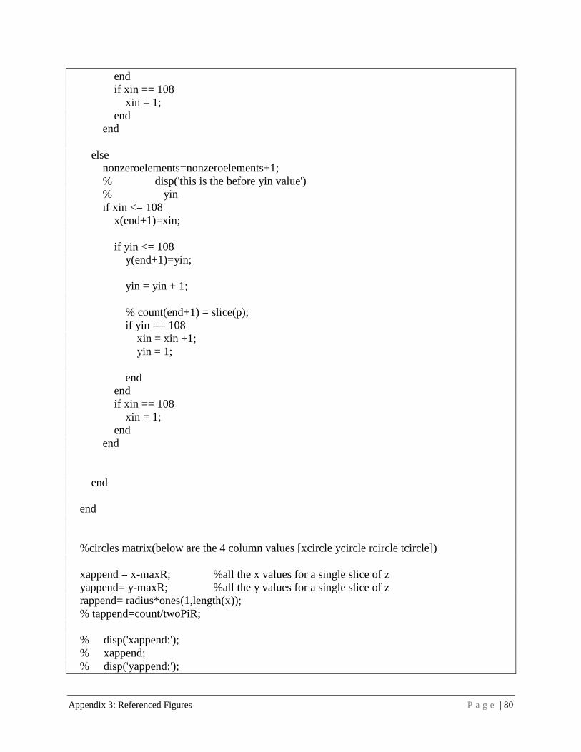
Appendix 3: Referenced Figures P a g e | 80
end
if xin == 108
xin = 1;
end
end
else
nonzeroelements=nonzeroelements+1;
% disp('this is the before yin value')
% yin
if xin <= 108
x(end+1)=xin;
if yin <= 108
y(end+1)=yin;
yin = yin + 1;
% count(end+1) = slice(p);
if yin == 108
xin = xin +1;
yin = 1;
end
end
if xin == 108
xin = 1;
end
end
end
end
%circles matrix(below are the 4 column values [xcircle ycircle rcircle tcircle])
xappend = x-maxR; %all the x values for a single slice of z
yappend= y-maxR; %all the y values for a single slice of z
rappend= radius*ones(1,length(x));
% tappend=count/twoPiR;
% disp('xappend:');
% xappend;
% disp('yappend:');

Appendix 3: Referenced Figures P a g e | 81
% yappend;
% disp('rappend:');
% rappend;
xcircle=[xcircle xappend];
ycircle=[ycircle yappend];
rcircle=[rcircle rappend];
%tcircle=[tcircle tappend];
stat = stat + 1;
end
% x
% disp('xappend')
% xappend
%
% disp('xcircle')
% xcircle
%
%
% disp('ycircle')
% ycircle
% ends the looping through the minR:maxR
% disp('slice at maxR')
% slice(maxR)
%size(xcircle)
% size(ycircle)
% size(rcircle)
% % % Collect candidate circles.
% % % Due to digitization, the number of detectable edge pixels are about 90%
% % % of the calculated perimeter.
% % twoPi = 0.9*2*pi;
% % circles = zeros(0,4); % Format: (x y r t)
% % for radius = minR:maxR % Loop from minimal to maximal radius
% % slice = hough(:,:,radius-minR+1); % Offset by minR
% % twoPiR = twoPi*radius;
% % slice(slice<twoPiR*thresh) = 0; % Clear pixel count < 0.9*2*pi*R*thresh
% % [y x count] = find(slice);
% % circles = [circles; [x-maxR, y-maxR, radius*ones(length(x),1), count/twoPiR]];
% % end
% %
% %
% % if nargout==0 % Draw circles
% % figure, imshow(origim), hold on;
% % for i = 1:size(circles,1)

Appendix 3: Referenced Figures P a g e | 82
% % x = circles(i,1)-circles(i,3);
% % y = circles(i,2)-circles(i,3);
% % w = 2*circles(i,3);
% % rectangle('Position', [x y w w], 'EdgeColor', 'red', 'Curvature', [1 1]);
% % end
% % hold off;
% % end
% %
%
% size(xcircle);
% size(ycircle);
% size(rcircle);
% size(tcircle);
%
%
% %if nargout==0 % Draw circles
zeroelements
nonzeroelements
%figure, imshow(origim),
hold on;
for i = 1:length(xcircle)
x1 = xcircle(i)-rcircle(i);
y1 = ycircle(i)-rcircle(i);
w1 = 2*rcircle(i);
plot(x1, y1,'+')
rectangle('Position', [x1 y1 w1 w1], 'EdgeColor', 'red', 'Curvature', [1 1]);
end
hold off;
% %end

Appendix 4: Embedded System P a g e | 83
Appendix 4: Embedded System
A4.1 System Generator Hardware: Entire Detection System
The following three sections (A4.1.1-A4.1.3) show the system below in greater detail.

Appendix 4: Embedded System P a g e | 84
A4.1.1 System Generator Hardware: Section 1 in Detail

Appendix 4: Embedded System P a g e | 85
A4.1.2 System Generator Hardware: Section 2 in Detail
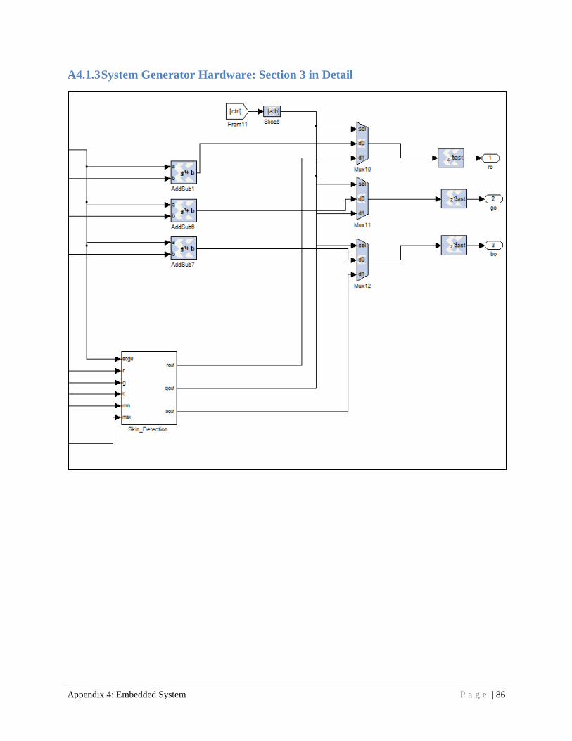
Appendix 4: Embedded System P a g e | 86
A4.1.3 System Generator Hardware: Section 3 in Detail

Appendix 5: Preload Function P a g e | 87
Appendix 5: Preload Function
A5.1 Still Image Edge Detection Preload Function % sysgenColorConverter_imageData is a matrix loaded by the model from a .mat
% file before this script is run.
% We now separate out the red green and blue components from the image.
redSignal = sysgenColorConverter_imageData(:,:,1);
greenSignal = sysgenColorConverter_imageData(:,:,2);
blueSignal = sysgenColorConverter_imageData(:,:,3);
NPixels = size(redSignal,1) * size(redSignal,2);
% turn them into vectors (they were arrays):
redSignal = reshape(redSignal,1,NPixels);
greenSignal = reshape(greenSignal,1,NPixels);
blueSignal = reshape(blueSignal,1,NPixels);
% insert a column of 'time values' in front -- the from workspace
% block expects time followed by data on every row of the input
redSignal = [ double(0:NPixels-1)' double(redSignal)'];
greenSignal = [ double(0:NPixels-1)' double(greenSignal)'];
blueSignal = [ double(0:NPixels-1)' double(blueSignal)'];
A5.2 Still Image Edge Detection Stop Function
if (exist('ySignal','var') & exist('NPixels','var'))
if ((~isempty(ySignal)))
designLatency = find(ySignal>0 & ySignal<1024);
if (isempty(designLatency))
return;
end
designLatency = designLatency(1);
imageSize = size(ySignal);
if (imageSize(1) >= designLatency+NPixels-1)
% The initial output of the design (pipeline stages)
% will be zeros and NaNs.
% For plotting, we just assume that the first non-zero, non-NaN
% output is the represents the first pixel.
h = Figure;
clf;
set(h,'Name',' Color Conversion Results');
set(h,'Position',[100 50 1000 800]);

P a g e | 88
ySignalN = ySignal(designLatency:designLatency+NPixels-1);
ySignalN = ySignalN - (min(ySignalN));
ySignalN = ySignalN / (max(ySignalN));
subplot(2,3,2);
image(sysgenColorConverter_imageData), ...
axis equal, axis square, axis off, title 'Original Image';
subplot(2,3,4);
image(reshape([ySignalN ySignalN ySignalN], ...
sqrt(NPixels),sqrt(NPixels),3)), ...
axis equal, axis square, axis off, title 'Grayscale';
prSignalN = prSignal(designLatency:designLatency+NPixels-1);
prSignalN = prSignalN - (min(prSignalN));
prSignalN = prSignalN / (max(prSignalN));
subplot(2,3,5);
image(reshape([prSignalN prSignalN prSignalN], ...
sqrt(NPixels),sqrt(NPixels),3)), ...
axis equal, axis square, axis off, title 'PR Component';
pbSignalN = pbSignal(designLatency:designLatency+NPixels-1);
pbSignalN = pbSignalN - (min(pbSignalN));
pbSignalN = pbSignalN / (max(pbSignalN));
subplot(2,3,6);
image(reshape([pbSignalN pbSignalN pbSignalN], ...
sqrt(NPixels),sqrt(NPixels),3)), ...
axis equal, axis square, axis off, title 'PB Component';
end
end
end

Appendix 6: Source Code P a g e | 89
Appendix 6: Source Code
A6.1 VSK Processing_Menu Header #include "xbasic_types.h"
#define VOP_BAYER_BYPASS 0
#define VOP_BAYER_PHASE0 0x11b41e4
#define VOP_BAYER_PHASE1 0x1b1144e
#define VOP_BAYER_PHASE2 0x14e14b4
#define VOP_BAYER_PHASE3 0x1e4411b
#define VOP_GAMMA_BYPASS 0
#define VOP_GAMMA_R709 1
Xint32 vsk_processing_menu (void);
Xint32 vsk_processing_bayer(Xuint32);
Xint32 vsk_processing_gamma(Xuint32);
Xint32 vsk_processing_dynamic_range(Xuint32);
Xint32 vsk_processing_init(void);
A6.2 VSK Processing Menu #include "vsk_processing_menu.h"
#include "vsk_processing_menu_l.h"
Xint32 vsk_processing_menu (void) {
Xint32 inchar;
Xint32 phase = 0;
static Xuint8 color = COL_RED;
static Xuint32 gamma = 1, bayer_phase = 0, spc_thresh = 96, spc_on = 1;
xc_iface_t *iface;
xc_to_reg_t *to_reg;
uint32_t tmp;
Xint32 ret = 0;
// initialize the software driver
xc_create(&iface,
&VSK_CAMERA_VOP_PLBW_ConfigTable[XPAR_VSK_CAMERA_VOP_PLBW_0_DEVICE_ID]);
vsk_processing_menu_help();
while (!ret)
{
print(">");
inchar = inbyte();
xil_printf("%c\n\r",inchar);
switch (inchar){
case '?' :
{
vsk_processing_menu_help();

Appendix 6: Source Code P a g e | 90
break;
}
case 0x1b :
{
xil_printf("- exit menu -\n\n\r");
ret = 1;
break;
}
case 'p' :
{
// Get reference to register
xc_get_shmem(iface, "spc_thresh", (void **) &to_reg);
if(spc_on == 1) {
tmp = 0xFFF; // set to max for off
spc_on = 0;
printf("Stuck pixel correction is off\r\n");
} else {
spc_on = 1;
tmp = spc_thresh;
printf("Stuck pixel correction is on\r\n");
}
xc_write(iface, to_reg->din, (const unsigned)tmp);
break;
}
case '.' :
{
// Get reference to register
xc_get_shmem(iface, "spc_thresh", (void **) &to_reg);
if (spc_thresh < 0xFFF) spc_thresh = spc_thresh + 16;
if (spc_thresh > 0xFFF) spc_thresh = 0xFFF; // clamp to max
xc_write(iface, to_reg->din, (const unsigned)spc_thresh);
xil_printf("Stuck pixel threshold set to %d\r\n", spc_thresh);
spc_on = 1; // Make sure software has correct state
break;
}
case ',' :
{
// Get reference to register
xc_get_shmem(iface, "spc_thresh", (void **) &to_reg);
if (spc_thresh == 0xFFF) spc_thresh = spc_thresh + 1; // boundary condition
if (spc_thresh > 0) spc_thresh = spc_thresh - 16;
xc_write(iface, to_reg->din, (const unsigned)spc_thresh);
xil_printf("Stuck pixel threshold set to %d\r\n", spc_thresh);
spc_on = 1; // Make sure software has correct state
break;
}
case 'y' :
{
if(bayer_phase < 3) bayer_phase++;
else bayer_phase = 0;
switch(bayer_phase) {
case 0:
vsk_processing_bayer(VOP_BAYER_PHASE0);
break;
case 1:

Appendix 6: Source Code P a g e | 91
vsk_processing_bayer(VOP_BAYER_PHASE1);
break;
case 2:
vsk_processing_bayer(VOP_BAYER_PHASE2);
break;
case 3:
vsk_processing_bayer(VOP_BAYER_PHASE3);
}
xil_printf("Bayer phase set to %d\r\n", bayer_phase);
break;
}
case 'h' : //Brightness on/off
{
xc_get_shmem(iface, "bc_ctrl", (void **) &to_reg);
xc_read(iface, to_reg->din, &tmp);
if(tmp & VOP_BC_BRIGHT_EN)
{
tmp &= ~VOP_BC_BRIGHT_EN;
print("Brightness control off\r\n");
}
else
{
tmp |= VOP_BC_BRIGHT_EN;
print("Brightness control on\r\n");
}
xc_write(iface, to_reg->din, (const unsigned)tmp);
break;
}
case 'n' : //Contrast on/off
{
xc_get_shmem(iface, "bc_ctrl", (void **) &to_reg);
xc_read(iface, to_reg->din, &tmp);
if(tmp & VOP_BC_CONT_EN)
{
tmp &= ~VOP_BC_CONT_EN;
print("Contrast control off\r\n");
}
else
{
tmp |= VOP_BC_CONT_EN;
print("Contrast control on\r\n");
}
xc_write(iface, to_reg->din, (const unsigned)tmp);
break;
}
case '1' : //overlay on/off
{
xc_get_shmem(iface, "bal_ctrl", (void **) &to_reg);
xc_read(iface, to_reg->din, &tmp);
if (tmp & 0x80) //if overlay is currently on
{
tmp ^= 0x80; //XOR with hex value to turn off
xil_printf("Overlay is off\r\n");

Appendix 6: Source Code P a g e | 92
}
else //if overlay is currently off
{
tmp ^= 0x80; //XOR with hex value to turn on
xil_printf("Overlay is on\r\n");
}
//write value to register
xc_write(iface, to_reg->din, (const unsigned)tmp);
break;
}
case '2' : //Sobel X on/off
{
xc_get_shmem(iface, "bal_ctrl", (void **) &to_reg);
xc_read(iface, to_reg->din, &tmp);
if(tmp & 0x80 && tmp ^ 0x40) //if overlay on
{
tmp ^= 0xC0; //XOR with hex
value..turns overlay off Sobel X on
xil_printf("Sobel X is on\r\n");
}
else if (tmp & 0x20 && tmp & 0x40) //If Sobel X and Y are both on
{
tmp ^= 0x20; //Turn Y
off
xil_printf("Sobel X is on\r\n");
}
else if (tmp ^ 0x40 && tmp & 0x20) //If Sobel X is off and Sobel Y is on
{
tmp ^= 0x60; //Turn
on X and Y off
xil_printf("Sobel X is on\r\n");
}
else if (tmp & 0x40) //If Sobel X on
{
tmp ^= 0x40; //Turn
Sobel X off
xil_printf("Sobel X is off\r\n");
}
else
{
tmp ^= 0x40; //Turn
Sobel X on
xil_printf("Sobel X is on\r\n");
}
//write value to register
xc_write(iface, to_reg->din, (const unsigned)tmp);
break;
}
case '3' : //Sobel Y on/off
{
xc_get_shmem(iface, "bal_ctrl", (void **) &to_reg);
xc_read(iface, to_reg->din, &tmp);

Appendix 6: Source Code P a g e | 93
if (tmp & 0x80 && tmp ^ 0x20) //If overlay on and Y off
{
tmp ^= 0xA0; //XOR with hex
value..turns overlay off and Y on
xil_printf("Sobel Y is on\r\n");
}
else if (tmp & 0x40 && tmp & 0x20) //X and Y both on
{
tmp ^= 0x40; //Turn X
off
xil_printf("Sobel Y is on\r\n");
}
else if (tmp ^ 0x20 && tmp & 0x40) //X on and Y off
{
tmp ^= 0x60; //Turn x off and y
on
xil_printf("Sobel Y is on\r\n");
}
else if (tmp & 0x20) //Y on
{
tmp ^= 0x20; //Turn Y
off
xil_printf("Sobel Y is off\r\n");
}
else
{
tmp ^= 0x20; //Turn Y
on
xil_printf("Sobel Y is on\r\n");
}
//write value to register
xc_write(iface, to_reg->din, (const unsigned)tmp);
break;
}
case '4' : //combined on/off
{
xc_get_shmem(iface, "bal_ctrl", (void **) &to_reg);
xc_read(iface, to_reg->din, &tmp);
if (tmp & 0x40 && tmp & 0x20) //x and y both on
{
tmp ^= 0x60; //turn x and y off
xil_printf("Combined off\r\n");
}
else
{
tmp |= 0x60; //turn on x or y or both
xil_printf("Combined on\r\n");
}
//write value to register
xc_write(iface, to_reg->din, (const unsigned)tmp);
break;
}
case '5' : //smooth on/off

Appendix 6: Source Code P a g e | 94
{
xc_get_shmem(iface, "bal_ctrl", (void **) &to_reg);
xc_read(iface, to_reg->din, &tmp);
if (tmp & 0x10) //smooth on
{
tmp ^= 0x10; //turn smooth off
xil_printf("Smooth is off\r\n");
}
else
{
tmp ^= 0x10; //turn smooth on
xil_printf("Smooth is on\r\n");
}
xc_write(iface, to_reg->din, (const unsigned)tmp);
break;
}
case '6' : //theshold down
{
xc_get_shmem(iface, "bc_ctrl", (void **) &to_reg);
xc_read(iface, to_reg->din, &tmp);
tmp = tmp - 10; //subtract 10 from threshold value
xil_printf("Sobel edge threshold set to %d\r\n", tmp);
//write value to register
xc_write(iface, to_reg->din, (const unsigned)tmp);
break;
}
case '7' : //threshold up
{
xc_get_shmem(iface, "bc_ctrl", (void **) &to_reg);
xc_read(iface, to_reg->din, &tmp);
tmp = tmp + 10; //add 10 to threshold
xil_printf("Sobel edge threshold set to %d\r\n", tmp);
//write value to register
xc_write(iface, to_reg->din, (const unsigned)tmp);
break;
}
case '8' : //Reset threshold
{
xc_get_shmem(iface, "bc_ctrl", (void **) &to_reg);
xc_read(iface, to_reg->din, &tmp);
tmp = 70; //set threshold to default value
xil_printf("Sobel edge threshold set to %d\r\n", tmp);
//write value to register
xc_write(iface, to_reg->din, (const unsigned)tmp);
break;
}
case '9' : //skin detection on/off
{
xc_get_shmem(iface, "bal_ctrl", (void **) &to_reg);
xc_read(iface, to_reg->din, &tmp);
if (tmp & 0x04) //if skin detection on
{

Appendix 6: Source Code P a g e | 95
tmp ^= 0x04; //turn skin detection off
xil_printf("Skin Detection is off\r\n");
}
else
{
tmp ^= 0x04; //turn skin detection on
xil_printf("Skin Detection is on\r\n");
}
//write value to register
xc_write(iface, to_reg->din, (const unsigned)tmp);
break;
}
case '0' : //skin + edge on/off
{
xc_get_shmem(iface, "bal_ctrl", (void **) &to_reg);
xc_read(iface, to_reg->din, &tmp);
if (tmp & 0x02) //if skin + edge on
{
tmp ^= 0x02; //turn off edge
xil_printf("Skin Detection\r\n");
}
else
{
tmp ^= 0x02; //turn on edge + skin detection
xil_printf("Skin Detection + Edge\r\n");
}
//write value to register
xc_write(iface, to_reg->din, (const unsigned)tmp);
break;
}
case '-' : //Brighness decrease
{
xc_get_shmem(iface, "brightness", (void **) &to_reg);
xc_read(iface, to_reg->din, &tmp);
//Sign extend if necessary
if (tmp & 0x100) tmp |= ~0xFF;
if ((Xint32)tmp > -255) (Xint32)tmp--;
xc_write(iface, to_reg->din, (const unsigned)tmp);
xil_printf("Brightness=%d\r\n", (Xint32)tmp);
break;
}
case '=' : //Brighness increase
{
xc_get_shmem(iface, "brightness", (void **) &to_reg);
xc_read(iface, to_reg->din, &tmp);
//Sign extend if necessary
if (tmp & 0x100) tmp |= ~0xFF;
if ((Xint32)tmp < 255) (Xint32)tmp++;
xc_write(iface, to_reg->din, (const unsigned)tmp);
xil_printf("Brightness=%d\r\n", (Xint32)tmp);
break;
}

Appendix 6: Source Code P a g e | 96
case 's' : //Show image stats
{
//First disabe stats so values read out are frame coherent
xc_get_shmem(iface, "stat_ctrl", (void **) &to_reg);
xc_write(iface, to_reg->din, ~VOP_STAT_EN);
//Read out stats
//Red
xc_get_shmem(iface, "r_min_val", (void **) &to_reg);
xc_read(iface, to_reg->din, &tmp);
xil_printf("Red:\tMin:\t%d", tmp);
xc_get_shmem(iface, "r_max_val", (void **) &to_reg);
xc_read(iface, to_reg->din, &tmp);
xil_printf("\tMax:\t%d\r\n", tmp);
//Green
xc_get_shmem(iface, "g_min_val", (void **) &to_reg);
xc_read(iface, to_reg->din, &tmp);
xil_printf("Green:\tMin:\t%d", tmp);
xc_get_shmem(iface, "g_max_val", (void **) &to_reg);
xc_read(iface, to_reg->din, &tmp);
xil_printf("\tMax:\t%d\r\n", tmp);
//Blue
xc_get_shmem(iface, "b_min_val", (void **) &to_reg);
xc_read(iface, to_reg->din, &tmp);
xil_printf("Blue:\tMin:\t%d", tmp);
xc_get_shmem(iface, "b_max_val", (void **) &to_reg);
xc_read(iface, to_reg->din, &tmp);
xil_printf("\tMax:\t%d\r\n", tmp);
//Re-enable stats so they will continue to calculate
xc_get_shmem(iface, "stat_ctrl", (void **) &to_reg);
xc_write(iface, to_reg->din, VOP_STAT_EN);
break;
}
case '[' : //Contrast decrease
{
xc_get_shmem(iface, "contrast", (void **) &to_reg);
xc_read(iface, to_reg->din, &tmp);
if (tmp > 0) tmp--;
xc_write(iface, to_reg->din, (const unsigned)tmp);
xil_printf("Contrast=%d.%03d\r\n", tmp>>to_reg->bin_pt,
(Xint32)((float)((tmp & ((1<<to_reg->bin_pt)-1))*1000)/(float)(1<<to_reg-
>bin_pt)));
break;
}
case ']' : //Contrast increase
{
xc_get_shmem(iface, "contrast", (void **) &to_reg);
xc_read(iface, to_reg->din, &tmp);
if (tmp < 255) tmp++;
xc_write(iface, to_reg->din, (const unsigned)tmp);
xil_printf("Contrast=%d.%03d\r\n", tmp>>to_reg->bin_pt,
(Xint32)((float)((tmp & ((1<<to_reg->bin_pt)-1))*1000)/(float)(1<<to_reg-
>bin_pt)));
break;
}
case 'r' : //Select color red
{

Appendix 6: Source Code P a g e | 97
color = COL_RED;
print("Red color selected\r\n");
break;
}
case 'g' : //Select color green
{
color = COL_GRN;
print("Green color selected\r\n");
break;
}
case 'b' : //Select color blue
{
color = COL_BLU;
print("Blue color selected\r\n");
break;
}
case ';' : //Color gain decrease
{
xc_get_shmem(iface, VopGainInfo[color].sm_name, (void **) &to_reg);
xc_read(iface, to_reg->din, &tmp);
if (tmp > 0) tmp--;
xc_write(iface, to_reg->din, (const unsigned)tmp);
xil_printf("%s Gain=%d.%03d\r\n", VopGainInfo[color].name, tmp>>to_reg->bin_pt,
(Xint32)((float)((tmp & ((1<<to_reg->bin_pt)-1))*1000)/(float)(1<<to_reg-
>bin_pt)));
break;
}
case '\'' : //Color gain increase
{
xc_get_shmem(iface, VopGainInfo[color].sm_name, (void **) &to_reg);
xc_read(iface, to_reg->din, &tmp);
if (tmp < 255) tmp++;
xc_write(iface, to_reg->din, (const unsigned)tmp);
xil_printf("%s Gain=%d.%03d\r\n", VopGainInfo[color].name, tmp>>to_reg->bin_pt,
(Xint32)((float)((tmp & ((1<<to_reg->bin_pt)-1))*1000)/(float)(1<<to_reg-
>bin_pt)));
break;
}
case 'o' : // Gamma enable/disable
{
if(gamma == VOP_GAMMA_BYPASS)
{
gamma = VOP_GAMMA_R709; // flip gamma setting
print("Gamma configured per Rec. 709.\r\n");
}
else
{
gamma = VOP_GAMMA_BYPASS; // flip gamma setting
print("Gamma configured as pass-through.\r\n");
}
vsk_processing_gamma(gamma);
break;
}
case 'i' : // Restore defaults
{
if (vsk_processing_init() == 0) {

Appendix 6: Source Code P a g e | 98
print("Processing settings successfully initialized.\r\n");
} else {
print("An error occurred while trying to initialize processing settings.\r\n");
}
break;
}
}
}
return 0;
}
void vsk_processing_menu_help(void)
{
print("\n\rEDGE DETECTION MENU\n\r");
print("----------------------------------\n\r");
print("key(s) description \n\r");
print("----------------------------------\n\r");
print(" 1 Overlay on/off\r\n");
print(" 2 Sobel X on/off\r\n");
print(" 3 Sobel Y on/off\r\n");
print(" 4 Combined on/off\r\n");
print(" 5 Smoothing Filter on/off\r\n");
print(" 6 Decrease Sobel Threshold on/off\r\n");
print(" 7 Increase Sobel Threshold on/off\r\n");
print(" 8 Restore Threshold Default on/off\r\n");
print(" 9 Skin Detection on/off\r\n");
print(" 0 Skin + Edge Detection on/off\r\n");
print(" esc Exit back to the Top-Level menu\r\n");
print(" ? help \n\r");
print("---------------------------------\n\r");
}
/* Set Bayer filter phase
* Returns 0 if phase was set successfully, otherwise not
*/
Xint32 vsk_processing_bayer(Xuint32 phase) {
xc_status_t status = XC_FAILURE;
xc_iface_t *iface;
xc_to_reg_t *bayer_reg;
// initialize the software driver
xc_create(&iface,
&VSK_CAMERA_VOP_PLBW_ConfigTable[XPAR_VSK_CAMERA_VOP_PLBW_0_DEVICE_ID]);
// Get reference to register
xc_get_shmem(iface, "bayer_ctrl", (void **) &bayer_reg);
switch(phase) {
case VOP_BAYER_PHASE0:
case VOP_BAYER_PHASE1:
case VOP_BAYER_PHASE2:
case VOP_BAYER_PHASE3:
case VOP_BAYER_BYPASS:
{
//status = vsk_camera_vop_sm_0_Write(
VSK_CAMERA_VOP_SM_0_BAYER_CTRL, VSK_CAMERA_VOP_SM_0_BAYER_CTRL_DIN,phase );
status = xc_write(iface, bayer_reg->din, (const unsigned) phase);

Appendix 6: Source Code P a g e | 99
#ifdef DEBUG
if(status == XC_FAILURE) { print("Error Writing to
VSK_Camera_VOP/Bayer_Ctrl\n\r"); }
#endif
}
}
return (status == XC_FAILURE ? 1 : 0);
}
/* Sets gamma table for red, green, and blue components
* When input VOP_GAMMA_BYPASS, gamma is set for 1-1 mapping
* When input VOP_GAMMA_R709, gamma is set using pre-calculated table
* Returns 0 on success,
*/
Xint32 vsk_processing_gamma(Xuint32 mode) {
Xuint32 i;
Xuint32 val;
Xuint32 address;
double x;
Xint32 retval = 1;
uint32_t current_buf;
uint32_t next_buf;
xc_status_t status;
xc_shram_t *shram_r;
xc_shram_t *shram_g;
xc_shram_t *shram_b;
xc_to_reg_t *gb_reg;
xc_iface_t *iface;
// initialize the software driver
xc_create(&iface, &GAMMA_PLBW_ConfigTable[XPAR_GAMMA_PLBW_0_DEVICE_ID]);
// obtain the memory location for storing the settings of the shared memory
xc_get_shmem(iface, "gamma_r", (void **) &shram_r);
xc_get_shmem(iface, "gamma_g", (void **) &shram_g);
xc_get_shmem(iface, "gamma_b", (void **) &shram_b);
xc_get_shmem(iface, "gamma_buffer", (void **) &gb_reg);
status = xc_read(iface, gb_reg->din, ¤t_buf);
if(status == XC_FAILURE) {
xil_printf("Error Reading from GAMMA_PLBW_0/Gamma_Buffer (%d)\n\r",status);
} else {
next_buf = (current_buf==0) ? 1 : 0;
if (mode == VOP_GAMMA_BYPASS)
{
status = XC_FAILURE;
for(i=0; i<256; i++)
{
address = (next_buf<<8) + i; // Push next_buf to bit location 9
status = xc_write(iface, xc_get_addr(shram_r->addr, address), (const unsigned) i);
if(status == XC_FAILURE) {
print("Error Writing to GAMMA_PLBW_0/GAMMA_R\n\r");
break;
}
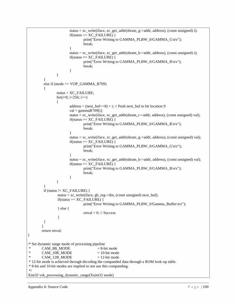
Appendix 6: Source Code P a g e | 100
status = xc_write(iface, xc_get_addr(shram_g->addr, address), (const unsigned) i);
if(status == XC_FAILURE) {
print("Error Writing to GAMMA_PLBW_0/GAMMA_G\n\r");
break;
}
status = xc_write(iface, xc_get_addr(shram_b->addr, address), (const unsigned) i);
if(status == XC_FAILURE) {
print("Error Writing to GAMMA_PLBW_0/GAMMA_B\n\r");
break;
}
}
}
else if (mode == VOP_GAMMA_R709)
{
status = XC_FAILURE;
for(i=0; i<256; i++)
{
address = (next_buf<<8) + i; // Push next_buf to bit location 9
val = gammaR709[i];
status = xc_write(iface, xc_get_addr(shram_r->addr, address), (const unsigned) val);
if(status == XC_FAILURE) {
print("Error Writing to GAMMA_PLBW_0/GAMMA_R\n\r");
break;
}
status = xc_write(iface, xc_get_addr(shram_g->addr, address), (const unsigned) val);
if(status == XC_FAILURE) {
print("Error Writing to GAMMA_PLBW_0/GAMMA_G\n\r");
break;
}
status = xc_write(iface, xc_get_addr(shram_b->addr, address), (const unsigned) val);
if(status == XC_FAILURE) {
print("Error Writing to GAMMA_PLBW_0/GAMMA_B\n\r");
break;
}
}
}
if (status != XC_FAILURE) {
status = xc_write(iface, gb_reg->din, (const unsigned) next_buf);
if(status == XC_FAILURE) {
print("Error Writing to GAMMA_PLBW_0/Gamma_Buffer\n\r");
} else {
retval = 0; // Success
}
}
}
return retval;
}
/* Set dynamic range mode of processing pipeline
* CAM_8B_MODE = 8-bit mode
* CAM_10B_MODE = 10-bit mode
* CAM_12B_MODE = 12-bit mode
* 12-bit mode is achieved through decoding the companded data through a ROM look-up table.
* 8-bit and 10-bit modes are implied to not use this companding.
*/
Xint32 vsk_processing_dynamic_range(Xuint32 mode)

Appendix 6: Source Code P a g e | 101
{
xc_status_t status = XC_FAILURE;
xc_iface_t *iface;
xc_to_reg_t *to_reg;
uint32_t tmp;
// initialize the software driver
xc_create(&iface,
&VSK_CAMERA_VOP_PLBW_ConfigTable[XPAR_VSK_CAMERA_VOP_PLBW_0_DEVICE_ID]);
// Get reference to register
xc_get_shmem(iface, "wdr_ctrl", (void **) &to_reg);
switch(mode)
{
case CAM_8B_MODE: // 8-bit mode, non-companding (pass-through enabled)
{
tmp = VOP_DR_PT_NCOMP_EN | VOP_DR_8B_N10B_EN;
break;
}
case CAM_10B_MODE: // 10-bit mode, non-companding (pass-through enabled)
{
tmp = VOP_DR_PT_NCOMP_EN | ((~VOP_DR_8B_N10B_EN) &
VOP_DR_8B_N10B_EN);
break;
}
case CAM_12B_MODE: // 12-bit mode (10-bit mode, companding enabled)
{
tmp = ((~VOP_DR_PT_NCOMP_EN) & VOP_DR_PT_NCOMP_EN) |
((~VOP_DR_8B_N10B_EN) &
VOP_DR_8B_N10B_EN);
}
}
status = xc_write(iface, to_reg->din, (const unsigned) tmp);
return (status == XC_FAILURE ? 1 : 0);
}
/* Initialize processing pipeline
return 0 on success, 1 on error
*/
Xint32 vsk_processing_init() {
Xint32 i;
xc_iface_t *iface;
xc_to_reg_t *to_reg;
Xint32 retval = 1;
// initialize the software driver
if (xc_create(&iface,
&VSK_CAMERA_VOP_PLBW_ConfigTable[XPAR_VSK_CAMERA_VOP_PLBW_0_DEVICE_ID]) !=
XC_FAILURE) {
for(i=0; i<NUM_DEF_PROC_PARAMS; i++) {
if (xc_get_shmem(iface, defProcParams[i].sm_name, (void **) &to_reg) !=
XC_FAILURE) {

Appendix 6: Source Code P a g e | 102
if (xc_write(iface, to_reg->din, (const unsigned)defProcParams[i].val) !=
XC_FAILURE) {
#ifdef DEBUG
xil_printf("Param[%s] = 0x%x\r\n", defProcParams[i].sm_name,
defProcParams[i].val);
#endif
retval = 0;
} else {
break;
}
} else {
break;
}
}
}
return retval;
}
A6.3 VSK Processing Menu_I Header #include <stdio.h>
// Located in: microblaze_0/include/
#include "xbasic_types.h"
#include "xutil.h"
#include "xparameters.h"
#include "gamma_plbw.h"
#include "vsk_camera.h"
#include "vsk_camera_vop_plbw.h"
#define VOP_DR_8B_N10B_EN 0x1 // When set dynamic range is 8-bit, else 10-bit
#define VOP_DR_PT_NCOMP_EN 0x2 // When set dynamic range is unchanged, else 12-bit
companding
#define VOP_BC_BRIGHT_EN 0x46
#define VOP_BC_CONT_EN 0x2
#define VOP_BAL_EN 0x80
#define VOP_STAT_EN 0x1
#define COL_RED 0
#define COL_GRN 1
#define COL_BLU 2
typedef struct {
Xint8 *sm_name;
Xint8 *name;
} VopGainStr;
static VopGainStr VopGainInfo[3] = {
// COL_RED
{
"r_bal",
"Red"
},
// COL_GRN

Appendix 6: Source Code P a g e | 103
{
"g_bal",
"Green"
},
// COL_BLU
{
"b_bal",
"Blue"
}
};
static Xuint8 gammaR709[256] = {
// ITU Recommendation 709 settings
0, 5, 9, 14, 18, 23, 27, 30,
34, 37, 40, 43, 46, 48, 51, 53,
55, 58, 60, 62, 64, 66, 68, 70,
72, 73, 75, 77, 78, 80, 82, 83,
85, 86, 88, 89, 91, 92, 94, 95,
97, 98, 99, 101, 102, 103, 104, 106,
107, 108, 109, 111, 112, 113, 114, 115,
116, 118, 119, 120, 121, 122, 123, 124,
125, 126, 127, 128, 129, 130, 131, 132,
133, 134, 135, 136, 137, 138, 139, 140,
141, 142, 143, 144, 145, 146, 147, 147,
148, 149, 150, 151, 152, 153, 154, 154,
155, 156, 157, 158, 159, 159, 160, 161,
162, 163, 164, 164, 165, 166, 167, 168,
168, 169, 170, 171, 171, 172, 173, 174,
174, 175, 176, 177, 177, 178, 179, 180,
180, 181, 182, 182, 183, 184, 185, 185,
186, 187, 187, 188, 189, 189, 190, 191,
191, 192, 193, 193, 194, 195, 195, 196,
197, 197, 198, 199, 199, 200, 201, 201,
202, 203, 203, 204, 205, 205, 206, 206,
207, 208, 208, 209, 209, 210, 211, 211,
212, 213, 213, 214, 214, 215, 216, 216,
217, 217, 218, 218, 219, 220, 220, 221,
221, 222, 223, 223, 224, 224, 225, 225,
226, 227, 227, 228, 228, 229, 229, 230,
230, 231, 232, 232, 233, 233, 234, 234,
235, 235, 236, 236, 237, 238, 238, 239,
239, 240, 240, 241, 241, 242, 242, 243,
243, 244, 244, 245, 245, 246, 246, 247,
247, 248, 248, 249, 249, 250, 251, 251,
252, 252, 253, 253, 254, 254, 255, 255
};
/* Default values for processing pipleine:
* spc_thresh = 0x60
* bc_ctrl = 0x3
* brightness = 0x0
* contrast = 0x80
* bal_ctrl = 0x1
* r_bal = 0x80
* g_bal = 0x80
* b_bal = 0x80

Appendix 6: Source Code P a g e | 104
*/
typedef struct {
Xint8 *sm_name;
Xuint32 val;
} DEF_PROC_PARAMS ;
#define NUM_DEF_PROC_PARAMS 9
static DEF_PROC_PARAMS defProcParams[NUM_DEF_PROC_PARAMS] = {
"spc_thresh", 0x60,
"bc_ctrl", VOP_BC_BRIGHT_EN | VOP_BC_CONT_EN,
"brightness", 0x0,
"contrast", 0x80,
"bal_ctrl", VOP_BAL_EN,
"r_bal", 0x80,
"g_bal", 0x80,
"b_bal", 0x80,
"stat_ctrl", VOP_STAT_EN
};
static void vsk_processing_menu_help(void);
A6.4 VSK_Top Header #include "xparameters.h"
// Size of input image
#define VID_IN_STRIDE 4096
#define VID_IN_WIDTH 720
#define VID_IN_HEIGHT 480
// Size of output image
#define VID_OUT_HEIGHT 480
#define VID_OUT_WIDTH 640
#define VID_OUT_STRIDE 2944 // 2560
// Frame buffer parameters
#define VID_FB_BASE_ADDR (XPAR_MPMC_0_MPMC_BASEADDR + 0x400000) // Give 4MB at
base of external memory for application
#define VID_FB_MAX_FRM_SIZE (VID_OUT_HEIGHT*VID_OUT_STRIDE)
#define VID_FB_MAX_SIZE ((XPAR_MPMC_0_MPMC_HIGHADDR -
VID_FB_BASE_ADDR) + 1)
A6.5 VSK_Top
#include <stdio.h>
#include <string.h>
// Located in: microblaze_0/include/
#include "xbasic_types.h"
#include "xutil.h"
#include "xparameters.h"

Appendix 6: Source Code P a g e | 105
#include "xstatus.h"
#include "vsk_iic.h"
#include "vsk_iic_diag.h"
#include "vsk_camera.h"
#include "vsk_dvi_out.h"
#include "vsk_fmc_video.h"
#include "vsk_iic_clock.h"
#include "vsk_util.h"
#include "video_to_vfbc.h"
#include "display_controller.h"
#include "vsk_camera_menu.h"
#include "vsk_processing_menu.h"
#include "vsk_storage_menu.h"
#include "vsk_top.h"
static void help_top(void);
XStatus main (void) {
Xint32 inchar;
XStatus status;
/* Initialize ICache */
microblaze_disable_icache();
microblaze_init_icache_range(XPAR_MICROBLAZE_0_ICACHE_BASEADDR,
XPAR_MICROBLAZE_0_CACHE_BYTE_SIZE);
microblaze_enable_icache ();
/* Initialize DCache */
microblaze_disable_dcache();
microblaze_init_dcache_range(XPAR_MICROBLAZE_0_DCACHE_BASEADDR,
XPAR_MICROBLAZE_0_DCACHE_BYTE_SIZE);
microblaze_enable_dcache ();
// Clear start of external memory (video buffers and BSS)
memset((void *)VID_FB_BASE_ADDR, 0, VID_FB_MAX_FRM_SIZE*3);
// Use white on black for terminal color scheme
print("\x1b[?5l\x1b[0m\x1b[H\x1b[J");
// Initialize the IIC cores
vsk_iic_init();
// Initialize the Power Regulator to provide 3.3v to the FMC
vsk_fmc_power_init();
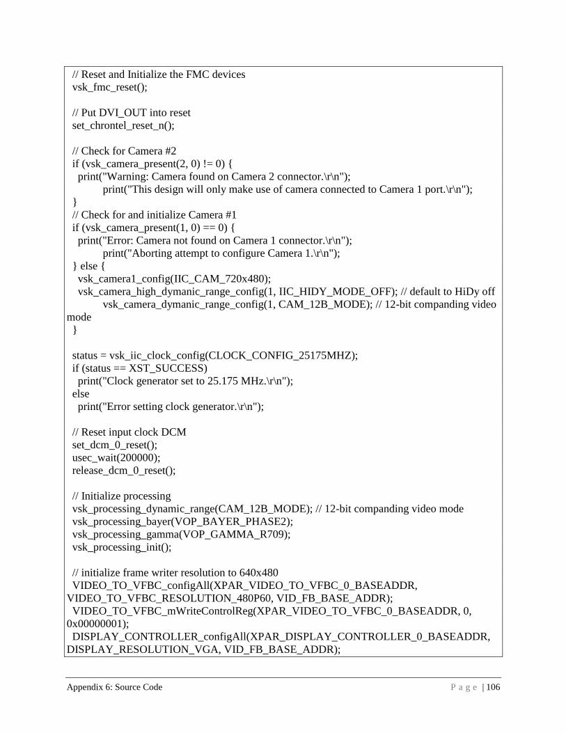
Appendix 6: Source Code P a g e | 106
// Reset and Initialize the FMC devices
vsk_fmc_reset();
// Put DVI_OUT into reset
set_chrontel_reset_n();
// Check for Camera #2
if (vsk_camera_present(2, 0) != 0) {
print("Warning: Camera found on Camera 2 connector.\r\n");
print("This design will only make use of camera connected to Camera 1 port.\r\n");
}
// Check for and initialize Camera #1
if (vsk_camera_present(1, 0) == 0) {
print("Error: Camera not found on Camera 1 connector.\r\n");
print("Aborting attempt to configure Camera 1.\r\n");
} else {
vsk_camera1_config(IIC_CAM_720x480);
vsk_camera_high_dymanic_range_config(1, IIC_HIDY_MODE_OFF); // default to HiDy off
vsk_camera_dymanic_range_config(1, CAM_12B_MODE); // 12-bit companding video
mode
}
status = vsk_iic_clock_config(CLOCK_CONFIG_25175MHZ);
if (status == XST_SUCCESS)
print("Clock generator set to 25.175 MHz.\r\n");
else
print("Error setting clock generator.\r\n");
// Reset input clock DCM
set_dcm_0_reset();
usec_wait(200000);
release_dcm_0_reset();
// Initialize processing
vsk_processing_dynamic_range(CAM_12B_MODE); // 12-bit companding video mode
vsk_processing_bayer(VOP_BAYER_PHASE2);
vsk_processing_gamma(VOP_GAMMA_R709);
vsk_processing_init();
// initialize frame writer resolution to 640x480
VIDEO_TO_VFBC_configAll(XPAR_VIDEO_TO_VFBC_0_BASEADDR,
VIDEO_TO_VFBC_RESOLUTION_480P60, VID_FB_BASE_ADDR);
VIDEO_TO_VFBC_mWriteControlReg(XPAR_VIDEO_TO_VFBC_0_BASEADDR, 0,
0x00000001);
DISPLAY_CONTROLLER_configAll(XPAR_DISPLAY_CONTROLLER_0_BASEADDR,
DISPLAY_RESOLUTION_VGA, VID_FB_BASE_ADDR);

Appendix 6: Source Code P a g e | 107
DISPLAY_CONTROLLER_setBufferAddresses(XPAR_DISPLAY_CONTROLLER_0_BASE
ADDR, DISPLAY_RESOLUTION_480P60, VID_FB_BASE_ADDR);
DISPLAY_CONTROLLER_mWriteReg(XPAR_DISPLAY_CONTROLLER_0_BASEADDR,
DISPLAY_CONTROLLER_CONTROL_OFFSET, 0x00000000);
// Initialize the DVI_OUT
release_chrontel_reset_n();
vsk_dvi_out_config(IIC_DVI_OUT);
vsk_dvi_out_display_present(1);
//Init SysACE controller
vsk_storage_init();
// Wait for user to continue
print("---- Press Any Key To Continue ----\r\n");
inbyte();
help_top();
while (1)
{
print(">");
inchar = inbyte();
xil_printf("%c\n\r",inchar);
switch (inchar){
case '?' :
{
help_top();
break;
}
case 'c' :
{
vsk_camera_menu();
help_top();
break;
}
case 'e' :
{
vsk_processing_menu();
help_top();
break;
}

Appendix 6: Source Code P a g e | 108
case 's' :
{
vsk_storage_menu();
help_top();
break;
}
case 'i' :
{
vsk_iic_diag_main();
help_top();
break;
}
}
}
}
static void help_top(void)
{
print("\n\r");
print("-----------------------------------------------------------------\n\r");
print("-------- MICHIGAN STATE UNIVERSITY ECE 480 DESIGN TEAM 3 --------\n\r");
print("-----------------------------------------------------------------\n\r");
print("--------------------- ++++++++++ -----------------------------\n\r");
print("--------------------- ++++++++++++ -----------------------------\n\r");
print("--------------------- ++++ ++++ -----------------------------\n\r");
print("--------------------- ++++ ++++ -----------------------------\n\r");
print("--------------------- ++++ -----------------------------\n\r");
print("--------------------- +++++++++++ -----------------------------\n\r");
print("--------------------- +++++++++++ -----------------------------\n\r");
print("--------------------- ++++ -----------------------------\n\r");
print("--------------------- ++++ ++++ -----------------------------\n\r");
print("--------------------- ++++ ++++ -----------------------------\n\r");
print("--------------------- ++++++++++++ -----------------------------\n\r");
print("--------------------- ++++++++++ -----------------------------\n\r");
print("-----------------------------------------------------------------\n\r");
print("--- FPGA IMPLEMENATION OF DRIVER ASSISTANCE CAMERA ALGORITHMS
---\n\r");
print("-----------------------------------------------------------------\n\r");
print("\n\r");
print(" e ENTER EDGE DETECTION MENU\r\n");
print("\n\r");
print("------------------------------------------------------\n\r");
}


![Dual-Mode FPGA Implementation of Target and Anomaly ... · implementation of target and anomaly detection algorithms in FPGA architectures [26]. Specifically, Chapter 15 in [26]](https://img.pdfslide.us/doc/110x75/5f0280d07e708231d40495b3/dual-mode-fpga-implementation-of-target-and-anomaly-implementation-of-target.jpg)