Embed Size (px)
Citation preview
University of New MexicoUNM Digital Repository
Electrical and Computer Engineering ETDs Engineering ETDs
6-9-2016
FPGA IMPLEMENTATION OF A REALTIMECYCLOSTATIONARY FEATURE DETECTORFOR OFDM SIGNALSSean Hamlin
Follow this and additional works at: https://digitalrepository.unm.edu/ece_etds
This Thesis is brought to you for free and open access by the Engineering ETDs at UNM Digital Repository. It has been accepted for inclusion inElectrical and Computer Engineering ETDs by an authorized administrator of UNM Digital Repository. For more information, please [email protected].
Recommended CitationHamlin, Sean. "FPGA IMPLEMENTATION OF A REALTIME CYCLOSTATIONARY FEATURE DETECTOR FOR OFDMSIGNALS." (2016). https://digitalrepository.unm.edu/ece_etds/112

i
Sean Hamlin Candidate Electrical and Computer Engineering
Department This thesis is approved, and it is acceptable in quality and form for publication: Approved by the Thesis Committee: Dr. Christos Christodoulou, Chairperson Dr. Sudharman Jayaweera Dr. Manel Martinez-Ramon

ii
FPGA IMPLEMENTATION OF A REALTIME CYCLOSTATIONARY FEATURE DETECTOR
FOR OFDM SIGNALS
by
SEAN HAMLIN
BACHELOR OF SCIENCE-ELECTRICAL ENGINEERING WICHITA STATE UNIVERSITY, 2010
THESIS
Submitted in Partial Fulfillment of the Requirements for the Degree of
Master of Science
Electrical Engineering
The University of New Mexico Albuquerque, New Mexico
May, 2016
iii
FPGA IMPLEMENTATION OF A REALTIME
CYCLOSTATIONARY FEATURE DETECTOR
FOR OFDM SIGNALS
by
Sean Hamlin
B.S. Electrical Engineering, Wichita State University, 2010
M.S. Electrical Engineering, University of New Mexico, 2016
ABSTRACT
The demand for wireless connectivity has prompted regulatory authorities in the
United States to investigate spectrum sharing of the DSRC band with U-NII operators.
However, DSRC operation has public safety implications, and moreover, time-critical
requirements due to the vehicular nature of its application. The field of cognitive radio
has identified several sensing techniques for the identification of licensed operators in a
given band. This thesis explores cyclostationary detection techniques for primary users.
A method will be identified for the detection of the 802.11p OFDM modulation used for
DSRC communications. A test statistic will be given that is invariant to the signal noise
covariance to allow simple and robust operation. Finally, the detection algorithm will be
implemented in FPGA digital logic in order to demonstrate the methods ability to be
employed in a commercial radio chipset with minimum resource requirements, yet still
provide real-time detection.
iv
TABLE OF CONTENTS
LIST OF FIGURES .......................................................................................................... v
LIST OF TABLES .......................................................................................................... vii
INTRODUCTION TO COGNITIVE RADIO........................................ 1 CHAPTER 11.1 Overview of Cognitive Radio .......................................................................................... 1 1.2 DSRC Spectrum Sharing ................................................................................................. 1 1.3 Overview of Feature Detection Techniques ................................................................... 3
1.3.1 Energy Detectors ....................................................................................................................... 4 1.3.2 Matched Filters ......................................................................................................................... 7 1.3.3 Cyclostationary Detection ......................................................................................................... 7
CYCLOSTATIONARY SIGNAL ANALYSIS .................................... 11 CHAPTER 22.1 Introduction .................................................................................................................... 11 2.2 Cyclic Autocorrelation Function ................................................................................... 11 2.3 Spectral Correlation Function ...................................................................................... 13 2.4 Spectral Coherence Function ........................................................................................ 19
OFDM FEATURE DETECTION .......................................................... 20 CHAPTER 33.1 OFDM Overview ............................................................................................................ 20 3.2 DSRC Modulation .......................................................................................................... 22 3.3 802.11p Simulation Model ............................................................................................. 27 3.4 OFDM Features for Cyclostationary Detection .......................................................... 28
3.4.1 Preamble ................................................................................................................................. 30 3.4.2 Pilots ....................................................................................................................................... 33 3.4.3 Cyclic Prefix ........................................................................................................................... 36
3.5 Detection of Cyclic Prefix with CAF ............................................................................ 38
DSRC DETECTION WITH CAF.......................................................... 41 CHAPTER 44.1 Spatial Sign Cyclic Correlation Estimator ................................................................... 41 4.2 Dual-Lag SSCCE with Cyclic Phase Compensation ................................................... 44 4.3 MATLAB Simulation ..................................................................................................... 45
4.3.1 Probability of Detection vs. SNR ............................................................................................ 46 4.3.2 ROC at Fixed SNR .................................................................................................................. 49 4.3.3 Histogram at Fixed SNR ......................................................................................................... 50
FPGA IMPLEMENTATION ................................................................. 51 CHAPTER 55.1 FPGA Overview ............................................................................................................. 51 5.2 SSCCE Algorithm Implementation .............................................................................. 53
5.2.1 Spatial Sign Function .............................................................................................................. 54 5.2.2 Lead/Lag Shift Register .......................................................................................................... 55 5.2.3 Multipliers ............................................................................................................................... 56 5.2.4 Numerically Controlled Oscillator .......................................................................................... 57 5.2.5 Moving Average Filter ............................................................................................................ 59
5.3 SSCCE Behavioral Simulation ...................................................................................... 60 5.4 SSCCE Resource Utilization ......................................................................................... 66 5.5 Conclusion ....................................................................................................................... 67
APPENDIX A MATLAB CODE ................................................................................... 69
APPENDIX B HDL CODE ............................................................................................ 74
REFERENCES .............................................................................................................. 100
v
LIST OF FIGURES
Figure 1.1 DSRC channel plan in the ITS band (from [5]). .............................................. 2
Figure 1.2 Proposed new UNII-4 band (from [5]). ............................................................ 3
Figure 1.3 Example of a receiver operating characteristic (ROC) curve. .......................... 6
Figure 1.4 (a) Power spectral density of lowpass signal. (b) Power spectral density of AM signal. (c) Power spectral density of squared lowpass signal. (d) Power spectral density of squared AM signal. ..................................................................... 10
Figure 2.1 Simplified block diagram of a spectrum analyzer for measuring the power spectral density at center frequency f (from [12]). .................................................... 15
Figure 2.2 Block diagram of a spectral correlation analyzer for center frequency f and cyclic frequency α (from [12]). ................................................................................ 16
Figure 2.3 Estimated spectral correlation density of an AM modulated signal with: (top) no additive noise, (middle) 5dB SNR, (bottom) -5dB SNR. .................................... 18
Figure 2.4 Contour of the estimated spectral correlation density of an AM modulated signal. ........................................................................................................................ 19
Figure 3.1 Simplified block diagram of an OFDM modulator and demodulator. ........... 22
Figure 3.2 DSRC channel plan (from [18]). .................................................................... 23
Figure 3.3 PPDU frame format (from [21]). .................................................................... 25
Figure 3.4 Time-domain plot an 802.11p PPDU frame of 10 symbols encoded with 64-QAM. ........................................................................................................................ 28
Figure 3.5 Power spectral density of an 802.11p PPDU frame of 100 symbols encoded with 64-QAM. ........................................................................................................... 29
Figure 3.6 Estimated spectral correlation density of an 802.11p PPDU frame. .............. 31
Figure 3.7 Contour of the estimated spectral correlation density of an 802.11p PPDU frame. ........................................................................................................................ 32
Figure 3.8 Contour of the estimated spectral correlation density of an 802.11p PPDU frame modified by replacing the pilot subcarriers with nulls. .................................. 34
Figure 3.9 Contour of the estimated spectral correlation density of an 802.11p PPDU frame modified by randomizing the pilot subcarriers. .............................................. 35
Figure 3.10 Estimated cyclic correlation density of an 802.11p PPDU frame. ............... 37
Figure 3.11 Autocorrelation function of an 802.11p PPDU frame. ................................. 38
Figure 4.1 Probability of detection vs. SNR of an 802.11p signal corrupted by an AWGN fading channel using SSCCE method with sample size of 1000. ............................. 48
Figure 4.2 Probability of detection vs. SNR of an 802.11p signal without additional impairments using SSCCE method with sample size of 1000. ................................. 48
vi
Figure 4.3 Receiver operating characteristic curve of the SSCCE method for an 802.11p signal. ........................................................................................................................ 49
Figure 4.4 Histogram of SSCCE test statistic for an 802.11p signal with -5dB SNR. .... 50
Figure 5.1 Flowchart of a typical FPGA design flow. ..................................................... 52
Figure 5.2 Block diagram of the FPGA implementation of the SSCCE algorithm. ........ 53
Figure 5.3 Block diagram showing the implementation of the SSF using CORDIC routines. ..................................................................................................................... 55
Figure 5.4 Block diagram showing the implementation of the lead/lag shift register. .... 56
Figure 5.5 Block diagram showing the implementation of a NCO using CORDIC........ 59
Figure 5.6 Screenshot of design simulation using Questa Sim. ....................................... 62
Figure 5.7 SSCCE algorithm probability of detection vs. SNR results from MATLAB simulation. ................................................................................................................. 63
Figure 5.8 SSCCE algorithm probability of detection vs. SNR from HDL implementation behavioral simulation. ..................................................................... 64
Figure 5.9 Difference in probability of detection between MATLAB simulation and HDL implementation. ............................................................................................... 64
Figure 5.10 RMSD of the SSCCE test statistic between MATLAB simulation and HDL implementation. ........................................................................................................ 65
Figure 5.11 Histogram of the first test statistic value to exceed the threshold for 5% Pfa. ................................................................................................................................... 65

vii
LIST OF TABLES
Table 1 OFDM PHY Modulation Parameters of 802.11p ............................................... 24
Table 2 Subcarrier Modulation Parameters of 802.11p ................................................... 26
Table 3 SSCCE Implementation Resource Utilization .................................................... 66
1
CHAPTER 1
INTRODUCTION TO COGNITIVE RADIO
1.1 Overview of Cognitive Radio
The demand on spectrum access has exploded within the past decade. Wireless
connectivity has seen rapid growth through 4G LTE, the ubiquity of Wi-Fi connection
hotspots, and the advent of LTE-A. Along with the incumbent spectrum users for LMR,
TV, radio, avionics and military communications, the ability to service all users will
become increasingly difficult with the current allocation schema. With this growing
strain on the wireless spectrum, interest in cognitive radio has transitioned from its
inception in the late 1990’s as a means to enhance the radio operator experience [1], to
legislative mandate by which the growing spectrum crisis can be mitigated [2].
Several definitions exist for the term cognitive radio. However, when discussed
in the context of spectrum sharing, perhaps the most germane description is that provided
by a spectrum regulating authority. According to the Federal Communications
Commission (FCC), cognitive radio is defined as an emerging technology of software
defined radios that monitor, sense, detect, and autonomously adapt their channel access to
suit the RF environment in which they are operating [3].
1.2 DSRC Spectrum Sharing
In 1999, the FCC licensed the 5.9 GHz band (5850-5925 MHz) for the purposes
of Dedicated Short Range Communications (DSRC) as an Intelligent Transportation
2
Systems radio service [4]. The intended purpose of this licensed spectrum is enhanced
transportation safety via Vehicle-to-Vehicle (V2V) and Vehicle-to-Infrastructure (V2I)
communications. Potential uses of DSRC are to alert drivers of approaching emergency
vehicles, blind spot, sudden braking, collision avoidance, adverse road conditions, as well
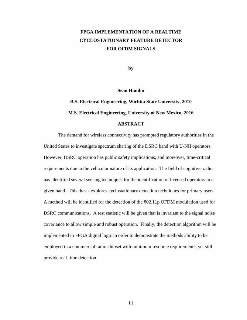
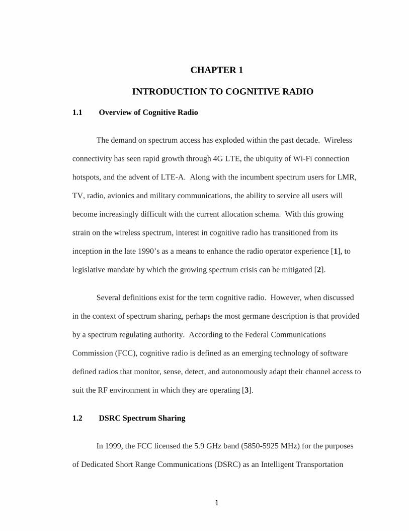
as traffic condition updates. Figure 1.1 shows the approved DSRC channel frequency
and power limit plan.
Figure 1.1 DSRC channel plan in the ITS band (from [5]).
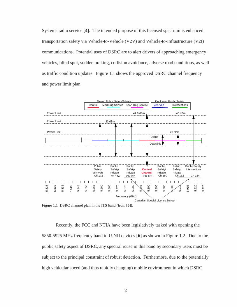
Recently, the FCC and NTIA have been legislatively tasked with opening the
5850-5925 MHz frequency band to U-NII devices [6] as shown in Figure 1.2. Due to the
public safety aspect of DSRC, any spectral reuse in this band by secondary users must be
subject to the principal constraint of robust detection. Furthermore, due to the potentially
high vehicular speed (and thus rapidly changing) mobile environment in which DSRC
Frequency (GHz)
5.85
0
5.85
5
5.86
0
5.86
5
5.87
0
5.87
5
5.88
0
5.88
5
5.89
0
5.89
5
5.90
0
5.90
5
5.91
0
5.91
5
5.92
0
5.92
5
5.82
5
5.83
0
5.83
5
5.84
0
5.84
5
Canadian Special License Zones*
Uplink
Downlink
Ch 172 Ch 174 Ch 176 Ch 180 Ch 184Ch 182Ch 178
PublicSafety/Private
Public SafetyIntersectionsControl
Channel
PublicSafety/Private
PublicSafety/Private
IntersectionsControl Veh-VehDedicated Public Safety
Short Rng ServiceMed Rng ServiceShared Public Safety/Private
PublicSafety/Private
PublicSafety
Veh-Veh
40 dBm
33 dBm
23 dBm
Power Limit
Power Limit
Power Limit
44.8 dBm
3
transceivers operate, secondary users must quickly detect primary users and relinquish
the spectrum. Additionally, given the nature of the currently identified secondary user
devices (802.11ac devices) the spectral detection mechanism must be power efficient and
consume minimum device resources in order to be commercially viable. Given these
constraints, the spectral detection and classification engine will likely reside in the radio
chipset of the secondary user device. This thesis will explore a new feature detection
technique, focused on the application of spectral reuse in the dedicated DSRC band for
802.11p primary users.
Figure 1.2 Proposed new UNII-4 band (from [5]).
1.3 Overview of Feature Detection Techniques
The scope of the term cognitive radio can include receiver side technologies for
detecting spectrum holes, channel estimation, and capacity prediction as well as
transmitter side technologies for transmitter power control and dynamic spectrum
management [7]. Arguably the main focus of cognitive radio is to enable the sharing of
DSRC

4
spectrum between licensed primary users and unlicensed secondary users. Towards this
end, spectrum sensing and signal detection techniques comprise a large portion of the
research in the field of cognitive radio [8].
In the field of cognitive radio, three primary signal detection techniques are
prominent, each with performance and design tradeoffs. These are energy based
detection, matched filter based detection, and cyclostationary based detection [8], [9].
1.3.1 Energy Detectors
Energy based detection is the simplest spectrum sensing technique. This
approach does not require knowledge of the primary signal and has a low implementation
complexity and computational cost. Energy based detectors simply compare the energy
of a receiver output against a threshold value. The threshold value is calculated
according to the level of noise in the received signal. In their simplest form, energy
detectors calculate a test statistic from N received samples as follows:
���� = 1��|�[�]| ������ ( 1 )
where the received signal is assumed to have the form:
�[�] = �[�] + �[�] ( 2 )
with �[�] being the primary signal to be detected and �[�] is additive white Guassian
noise. The goal of spectrum sensing algorithms is to form a decision as to the presence of

5
the primary signal. Therefore, the null hypothesis, that the primary signal is not present,
and its alternative are formulated as:
ℋ� : �[�] = �[�],ℋ� : �[�] = �[�] + �[�]. ( 3 )
A threshold value, �, is determined for the test statistic, above which the null hypothesis
is rejected. The performance of the energy detector to correctly detect the presence of the
primary signal (i.e. its sensitivity) is given as:
�� = �� !"���� > �|ℋ�% ( 4 )
Similarly, the performance of the detectors false alarm rate, that is the probability of
asserting the presence of a primary signal when it is not present (i.e. its specificity), is
given as:
�&' = �� !"���� > �|ℋ�% ( 5 )
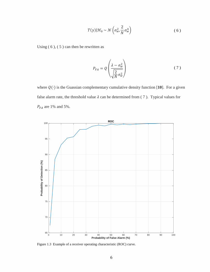
A receiver operating characteristic (ROC) curve is obtained by plotting the
probability of detection versus the probability of false alarm, an example of which is
shown in Figure 1.3. Naturally it is desired to maximize the probability of detection
while minimizing the probability of false alarm. The desired balance between probability
of detection and probability of false alarm is controlled by the threshold value �. In
order to determine the value of �, it is observed that the noise component �[�] is
assumed to be normally distributed with zero-mean and variance () . The distribution of
the test statistic ( 1 ) is then given as:
6
����|ℋ�~+ ,() , 2� ()./ ( 6 )
Using ( 6 ), ( 5 ) can then be rewritten as
�&' = 012� − () 42�() 5
6 ( 7 )
where 0�∙� is the Guassian complementary cumulative density function [10]. For a given
false alarm rate, the threshold value � can be determined from ( 7 ). Typical values for
�&' are 1% and 5%.
Figure 1.3 Example of a receiver operating characteristic (ROC) curve.
0 10 20 30 40 50 60 70 80 90 100Probability of False Alarm (%)
65
70
75
80
85
90
95
100
Pro
bab
ility
of
Det
ecti
on
(%
)
ROC

7
As can be seen from the above derivation, the presence of a signal is determined
by the energy detector with no apriori information about the primary signal. However,
there is also no distinction between a primary signal and interference or other secondary
signals. Furthermore, as can be seen from ( 7 ), knowledge of the noise power is required
to determine the optimal threshold value. It may also be observed that by averaging more
samples, an arbitrarily low signal-to-noise ratio could still allow for positive signal
detection. However, as shown in [10] any slight uncertainty in the knowledge of the
noise variance drastically affects the performance of the detection scheme below a certain
SNR, regardless of the number of samples averaged.
1.3.2 Matched Filters
Matched filters provide the optimal detection method for a known signal type.
These filters are created by correlating a known signal with the received signal, and are
optimal in the sense that they maximize the signal to noise ratio of the filter output.
Unfortunately, this method requires complete knowledge of the primary signal, and
demodulation of the same, in order to implement. For all but the most simple of
modulation types, this method entails a high-computational complexity.
1.3.3 Cyclostationary Detection
Cyclostationary processes are those whose statistical parameters vary periodically
as a function of time [11]. A common example is meteorological data, which has strong
periodicities according to the season. Many communications modulation and coding
schemes exhibit cyclostationarity as well.
8
Periodicity in signals can typically be found by visual inspection of either their
time series data or through spectral analysis. For example, a signal corrupted by noise,
8�9� = : cos�2>?9 + @� + ��9�, when subject to the linear transformation with the
Fourier kernel will produce spectral lines at A = ±?. In such case, regardless of the
noise component, the signal is said to contain first-order periodicity in frequency ? [12].
However, a time-series may contain other types of periodicities that do not produce
spectral lines. These signals are said to posses wide-sense cyclostationarity of order-n if
and only if there exists a non-linear time-invariant transformation of the time-series such
that the transformed time-series produces spectral lines [12]. Therefore, a signal contains
second-order periodicity (i.e. n=2) if its time-series undergoes a quadratic time-invariant
transformation
��9� = C C D�E, F�8�9 − E�8�9 − F�GEGFH�H
H�H ( 8 )
such that ��9� exhibits first-order periodicity in frequency ? [13]. Some possible
quadratic nonlinear time invariant transformation functions could be the squaring
operation on the time-series or the multiplication of the time-series with a time lagged
version of itself.
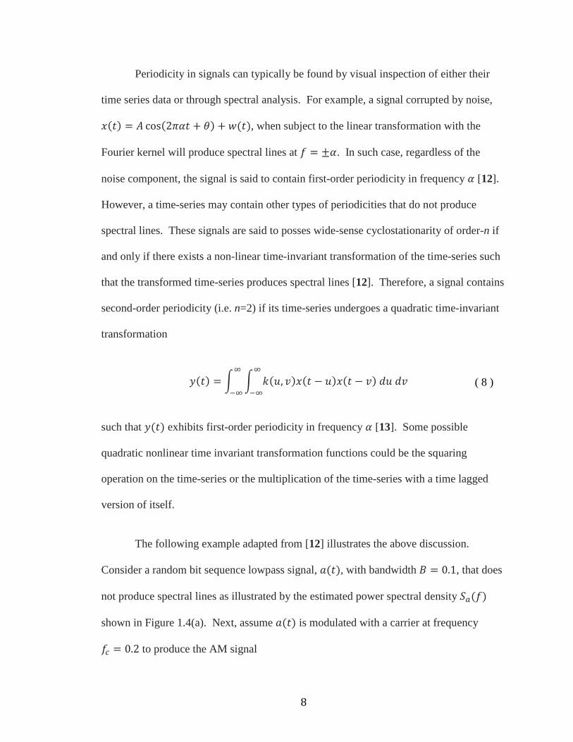
The following example adapted from [12] illustrates the above discussion.
Consider a random bit sequence lowpass signal, I�9�, with bandwidth J = 0.1, that does
not produce spectral lines as illustrated by the estimated power spectral density LM�A� shown in Figure 1.4(a). Next, assume I�9� is modulated with a carrier at frequency
AN = 0.2 to produce the AM signal
9
8�9� = I�9� cos�2>AN9�. ( 9 )
The resulting power spectral density LO�A� of the modulated signal is then
LO�A� = 14 [LM�A + AN� + LM�A − AN�], ( 10 )
whose estimate is shown in Figure 1.4(b). Observe that the power spectral density of the
modulated signal still does not contain any spectral lines. In order to test the modulated
signal for second-order periodicity, we use a squaring function as a quadratic time-
invariant transformation:
��9� = 8 �9� = I �9� + cos �2>AN9�= 12 [!�9� + !�9� cos�4>AN9�] ( 11 )
where
!�9� = I �9� ( 12 )
The squaring operation forces !�9� to be completely non-negative, boosting the
DC component, doubling the bandwidth of I�9� and leading to the spectral line at A = 0
shown Figure 1.4(c). The power spectral density of ( 11 ) is
LQ�9� = 14 RLS�A� + 14 LS�A + 2AN� + 14 LM�A − 2AN�T, ( 13 )
which is estimated in Figure 1.4(d). The quadratic transformation has therefore produced
first-order periodicity by revealing spectral lines at A = 0 and A = ±2AN. The next
chapter will explore cyclostationary methods in more depth.
10
Figure 1.4 (a) Power spectral density of lowpass signal. (b) Power spectral density of AM signal. (c) Power spectral density of squared lowpass signal. (d) Power spectral density of squared AM signal.
-0.5 -0.4 -0.3 -0.2 -0.1 0 0.1 0.2 0.3 0.4 0.5f
0
1
2
3
4S
a(f)
(a)
-0.5 -0.4 -0.3 -0.2 -0.1 0 0.1 0.2 0.3 0.4 0.5f
0
0.2
0.4
0.6
0.8
1S
x(f)
(b)
-0.5 -0.4 -0.3 -0.2 -0.1 0 0.1 0.2 0.3 0.4 0.5f
0
100
200
300S
b(f)
(c)
-0.5 -0.4 -0.3 -0.2 -0.1 0 0.1 0.2 0.3 0.4 0.5f
0
20
40
60
80S
y(f)
(d)
11
CHAPTER 2
CYCLOSTATIONARY SIGNAL ANALYSIS
2.1 Introduction
The previous chapter introduced the concept of cyclostationary time-series. For
signals of second-order periodicity, it was shown that a quadratic time-invariant
transformation could be used to create a time-series that exhibited first-order periodicity.
A simple example of such a transformation was given as the squaring operation.
However, the squaring operation is really an example of a more generalized quadratic
transformation as shown examination of ( 8 ). Specifically, any operation that measures
second-order moment (variance) is required. Two second-order measures are the
autocorrelation function in the time domain and the power spectrum transform in the
frequency domain. Therefore, the definition of wide-sense cyclostationary time-series
can be restated as one whose first-order measure (expectation value) and second-order
measure (autocorrelation function) are periodic with some period �� [11].
2.2 Cyclic Autocorrelation Function
From the definition of wide-sense cyclostationary time-series it is implied that for
all 9, U:
Ε[8�9 + ���] = Ε[8�9�] ( 14 )
WO�9 + ��, U� = WO�9, U� ( 15 )
12
where the autocorrelation function is defined as
WO�9, U� ≜ Ε[8∗�9 + U�8�9�]. ( 16 )
Because the autocorrelation function ( 16 ) is wide-sense stationary, ( 15 ) can be
simplified to only be a function of U:
WO�9, U� = WO�U�. ( 17 )
In order to show if a time-series exhibits second-order periodicity, it is then necessary to
see if the time-series that has undergone transformation via the autocorrelation function
generates spectral lines. The most intuitive test of first-order periodicity at a frequency ?
would be to determine the Fourier coefficient of the autocorrelation function at that
frequency [13]:
WOZ�U� ≜ lim^→H 1�C 8 `9 + U2a 8∗ `9 − U2a^ ⁄�^ ⁄ c�d eZfG9. ( 18 )
The above expression is referred to as the Cyclic Autocorrelation Function (CAF). Using
the CAF, 8�9� can be said to exhibit second-order cyclostationarity if and only if for
some nonzero value of ?, WOZ�U� ≠ 0, i.e. it contains a sine-wave component. The
frequency parameter ? is referred to as the cycle or cyclic frequency and implies that a
time-series with cyclostationary periodicity of �� has a nonzero CAF at cyclic frequency
? = 1 ��⁄ . Note, that for ? = 0 the CAF is the usual continuous-time autocorrelation
function.
13
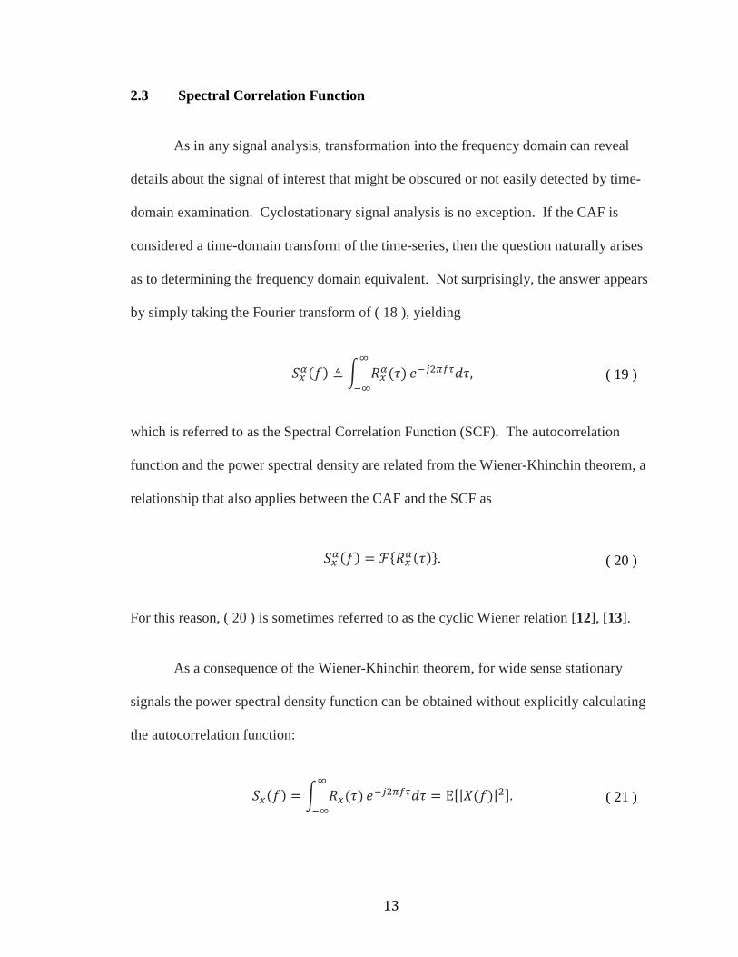
2.3 Spectral Correlation Function
As in any signal analysis, transformation into the frequency domain can reveal
details about the signal of interest that might be obscured or not easily detected by time-
domain examination. Cyclostationary signal analysis is no exception. If the CAF is
considered a time-domain transform of the time-series, then the question naturally arises
as to determining the frequency domain equivalent. Not surprisingly, the answer appears
by simply taking the Fourier transform of ( 18 ), yielding
LOZ�A� ≜ C WOZ�U�H�H c�d ehiGU, ( 19 )
which is referred to as the Spectral Correlation Function (SCF). The autocorrelation
function and the power spectral density are related from the Wiener-Khinchin theorem, a
relationship that also applies between the CAF and the SCF as
LOZ�A� = ℱ"WOZ�U�%. ( 20 )
For this reason, ( 20 ) is sometimes referred to as the cyclic Wiener relation [12], [13].
As a consequence of the Wiener-Khinchin theorem, for wide sense stationary
signals the power spectral density function can be obtained without explicitly calculating
the autocorrelation function:
LO�A� = C WO�U�H�H c�d ehiGU = Ε[|k�A�| ]. ( 21 )
14
The power spectrum density can then be estimated from time-smoothing of the finite-
time signal 8^�9� as follows
LO�A� = lim^→H LOl�A� = lim^→HΕ[|k^�A�| ]. ( 22 )
k^�A� can be estimated from the short-time Fourier transform
k^�9, A� = 1√�C 8�E�c�d ehnGEfo^ ⁄f�^ ⁄ . ( 23 )
The finite-time estimate of the power spectrum density is then
LOl�9, A�∆f = 1∆9C 1� k^�9 + E, A�k∗�9 + E, A�GE∆f ⁄�∆f ⁄ , ( 24 )
from which the power spectrum density is calculated according to the limits
LO�A� = lim^→H lim∆f→H LOl�9, A�∆f. ( 25 )
Graphically, ( 24 ) can be realized as the familiar spectrum analyzer, shown in Figure 2.1,
whose output yields the power spectrum density as the filter bandwidth J = 1 �⁄ → 0
and the observation time ∆9 → ∞
LO�A� = limr→� 1J stℎrv&�9� ∗ 8�9�t w. ( 26 )
15
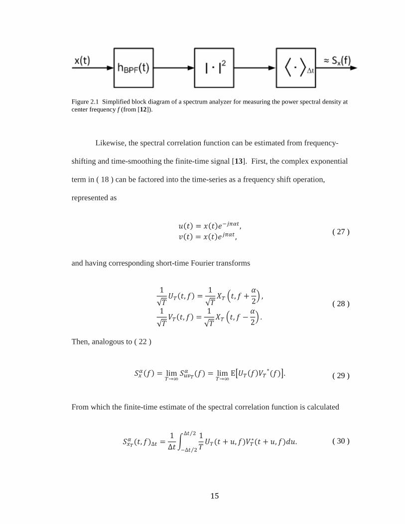
Figure 2.1 Simplified block diagram of a spectrum analyzer for measuring the power spectral density at center frequency f (from [12]).
Likewise, the spectral correlation function can be estimated from frequency-
shifting and time-smoothing the finite-time signal [13]. First, the complex exponential
term in ( 18 ) can be factored into the time-series as a frequency shift operation,
represented as
E�9� = 8�9�c�deZf,F�9� = 8�9�cdeZf, ( 27 )
and having corresponding short-time Fourier transforms
1√�x^�9, A� = 1√�k^ `9, A + ?2a ,1√� y �9, A� = 1√�k^ `9, A − ?2a . ( 28 )
Then, analogous to ( 22 )
LOZ�A� = lim^→H LnzlZ �A� = lim^→HΕ{x^�A�y ∗�A�|. ( 29 )
From which the finite-time estimate of the spectral correlation function is calculated
LOlZ �9, A�∆f = 1∆9C 1�x^�9 + E, A�y∗�9 + E, A�GE∆f ⁄�∆f ⁄ . ( 30 )
16
And finally yielding the spectral correlation function in the limits
LOZ�A� = lim^→H lim∆f→H LOlZ �9, A�∆f. ( 31 )
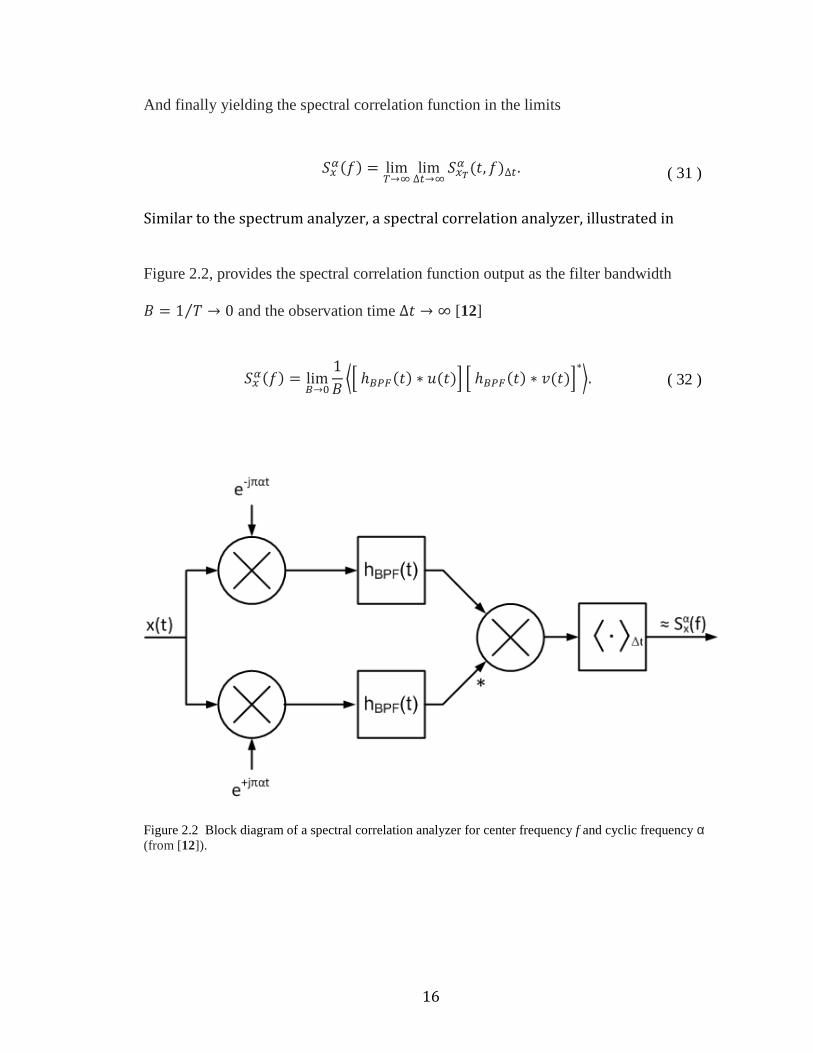
Similar to the spectrum analyzer, a spectral correlation analyzer, illustrated in
Figure 2.2, provides the spectral correlation function output as the filter bandwidth
J = 1 �⁄ → 0 and the observation time ∆9 → ∞ [12]
LOZ�A� = limr→� 1J s}ℎrv&�9� ∗ E�9�~ }ℎrv&�9� ∗ F�9�~∗w. ( 32 )
Figure 2.2 Block diagram of a spectral correlation analyzer for center frequency f and cyclic frequency α (from [12]).
17
Because the SCF allows visualization of a time-series in the bi-frequency plane
(cyclic frequency vs. spectral frequency), the cyclostationary parameters of multiple
incident signals can be examined simultaneously. Communications signals exhibit
cyclostationarity due to symbol rate, sampling rate, multiplexing, modulation, and coding
operations [11]. These cyclostationary effects manifest themselves in the SCF such that
many modulation types will present unique signatures in the bi-frequency plane, which
can aid in their identification. Additionally, because the SCF is a correlation of the
spectral components of the time-series, and white noise is uncorrelated, the SCF is
insensitive to the effects of additive white noise for cyclic frequencies other than zero
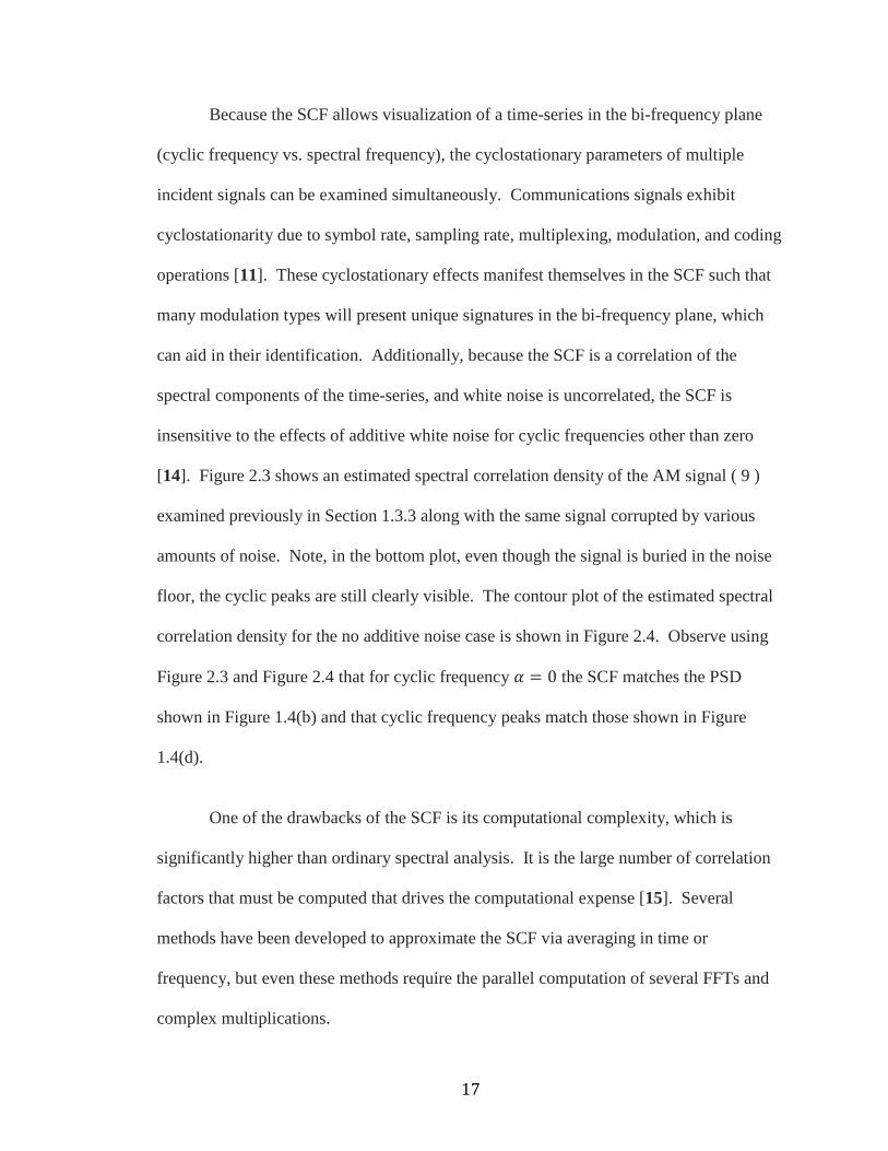
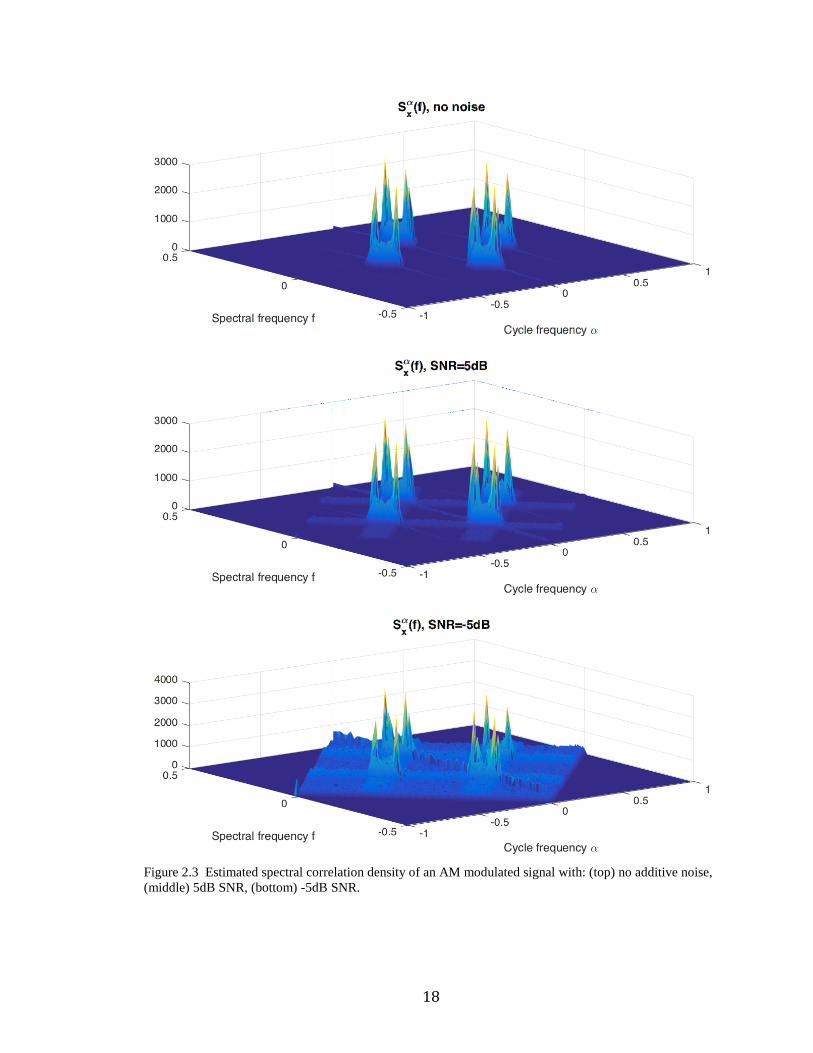
[14]. Figure 2.3 shows an estimated spectral correlation density of the AM signal ( 9 )
examined previously in Section 1.3.3 along with the same signal corrupted by various
amounts of noise. Note, in the bottom plot, even though the signal is buried in the noise
floor, the cyclic peaks are still clearly visible. The contour plot of the estimated spectral
correlation density for the no additive noise case is shown in Figure 2.4. Observe using
Figure 2.3 and Figure 2.4 that for cyclic frequency ? = 0 the SCF matches the PSD
shown in Figure 1.4(b) and that cyclic frequency peaks match those shown in Figure
1.4(d).
One of the drawbacks of the SCF is its computational complexity, which is
significantly higher than ordinary spectral analysis. It is the large number of correlation
factors that must be computed that drives the computational expense [15]. Several
methods have been developed to approximate the SCF via averaging in time or
frequency, but even these methods require the parallel computation of several FFTs and
complex multiplications.
18
Figure 2.3 Estimated spectral correlation density of an AM modulated signal with: (top) no additive noise, (middle) 5dB SNR, (bottom) -5dB SNR.
19
2.4 Spectral Coherence Function
Lastly, the SCF can be normalized to produce a proper coherence value, referred
to as the spectral coherence function (abbreviated SOF) with a magnitude in the range
[0,1], given as [14]
�OZ�A� = LOZ�A�{LO��A + Z �LOZ�A − Z �∗|� ⁄ . ( 33 )
Figure 2.4 Contour of the estimated spectral correlation density of an AM modulated signal.
20
CHAPTER 3
OFDM FEATURE DETECTION
3.1 OFDM Overview
Orthogonal frequency-division multiplexing (OFDM) is a digital modulation
scheme that is ideally suited for the transmission of data in multipath fading
environments. As data rates continue to increase, the symbol time of single-carrier
modulation methods becomes less than the channel impulse response time and which can
result in severe intersymbol interference (ISI) from multipath propagation. OFDM
instead utilizes multiple carriers to transmit the same aggregate data rate but at a lower
per carrier symbol rate, conceptually analogous to parallelizing a data bus to achieve the
same bandwidth as a much faster serial bus. The subcarriers are spaced orthogonally in
frequency according to the inverse of the data symbol time �&&^
∆A = 1�&&^ . ( 34 )
In this way, OFDM can achieve high-spectral efficiency by maintaining optimal spacing
between subcarriers. The subcarriers themselves can be modulated with any suitable
quadrature amplitude modulation encoding scheme.
The longer symbol times in OFDM modulation techniques make mitigation of
multipath propagation easier by the insertion of a sub-symbol time guard interval. This
guard interval is referred to as a cyclic prefix and consists of a portion of the end of the
OFDM symbol appended to the front of the symbol, the duration of which is chosen to be
longer than the channel impulse response. Typical lengths for the guard interval are ⅛ to
21
¼ of the symbol time. By copying the end of the symbol to its beginning and assuming
the channel impulse response is shorter than or equal to the length of the guard interval,
the linear convolution of the transmitted symbol with the channel response can be
modeled as a circular convolution. By assuming a flat fading model per subcarrier,
receiver equalization is then simplified to a one-tap equalizer for each subcarrier.
The concept of OFDM modulation has been known for some time, but only
recently has been exploited on a commercial basis with the advent of low-cost, high-
performance digital signal processors and application specific integrated circuits. OFDM
modulators and demodulators are efficiently implemented with the use of the Fast Fourier
Transform (FFT). In the case of the modulator, the inverse-FFT converts the parallel set
of mapped complex baseband data, which are conceptually in the frequency domain and
separated by the bin spacing of the IFFT, into a serial stream of time domain data. This
transformation of the baseband data from frequency domain to time domain has the effect
of modulating the baseband samples by their respective subcarriers. Not all of the
subcarriers may necessarily be used for modulating data. Depending on the modulation
type, some subcarriers may be assigned a pilot signal to assist the receiver in equalization
and other subcarriers may be null. Afterwards the cyclic prefix is appended to the
symbol before transmission. Note, due to the optimal spacing of the subcarriers, the
bandwidth of the OFDM transmission is related to the number of subcarriers, �&&^ and
the subcarrier spacing:
J� = �&&^ ∙ ∆A ( 35 )
22
An OFDM demodulator operates in reverse to the modulator. First, the cyclic
prefix is removed to obtain a symbol frame corresponding to the expected number of
subcarriers, which is then fed to an FFT. The FFT output bins represent the demodulated
data of each of the subcarriers. The output bins are equalized, de-mapped, and serialized
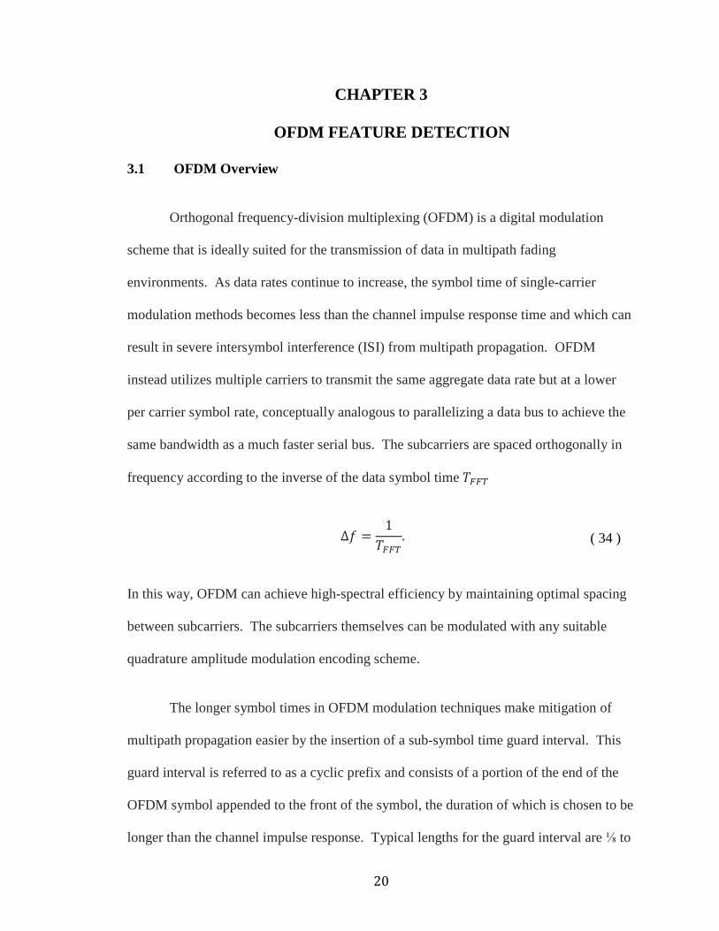
to provide the output data. Figure 3.1 presents a simplified block diagram of an OFDM
modulator and demodulator.
Figure 3.1 Simplified block diagram of an OFDM modulator and demodulator.
3.2 DSRC Modulation
Dedicated Short Range Communications (DSRC) is properly defined by ASTM
Standard E2213-03 and is identified as the 5.9 GHz band allocated for Intelligent
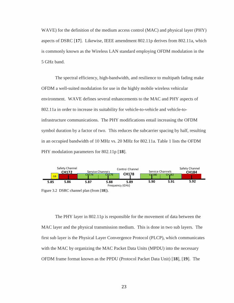
Transportation Systems (ITS) communications. The DSRC band consists of seven 10
MHz-wide channels starting at 5.855 GHz, shown in Figure 3.2 (a 5 MHz guard band
separates DSRC from the lower adjacent band) [16]. ASTM E2213-03 utilizes IEEE-
802.11p amendment (referred to as Wireless Access in Vehicular Environments—
23
WAVE) for the definition of the medium access control (MAC) and physical layer (PHY)
aspects of DSRC [17]. Likewise, IEEE amendment 802.11p derives from 802.11a, which
is commonly known as the Wireless LAN standard employing OFDM modulation in the
5 GHz band.
The spectral efficiency, high-bandwidth, and resilience to multipath fading make
OFDM a well-suited modulation for use in the highly mobile wireless vehicular
environment. WAVE defines several enhancements to the MAC and PHY aspects of
802.11a in order to increase its suitability for vehicle-to-vehicle and vehicle-to-
infrastructure communications. The PHY modifications entail increasing the OFDM
symbol duration by a factor of two. This reduces the subcarrier spacing by half, resulting
in an occupied bandwidth of 10 MHz vs. 20 MHz for 802.11a. Table 1 lists the OFDM
PHY modulation parameters for 802.11p [18].
Figure 3.2 DSRC channel plan (from [18]).
The PHY layer in 802.11p is responsible for the movement of data between the
MAC layer and the physical transmission medium. This is done in two sub layers. The
first sub layer is the Physical Layer Convergence Protocol (PLCP), which communicates
with the MAC by organizing the MAC Packet Data Units (MPDU) into the necessary
OFDM frame format known as the PPDU (Protocol Packet Data Unit) [18], [19]. The
Frequency (GHz)
CH172
5.85 5.86 5.87 5.88 5.89 5.915.90 5.92
CH178 CH184
Control Channel Safety Channel Safety Channel Service Channels Service Channels
CH174 CH176 CH180 CH182 GB
24
second sub layer is the Physical Medium Dependent (PMD). The PMD places the
PPDUs on the physical medium (RF in the case of DSRC applications).
Table 1 OFDM PHY Modulation Parameters of 802.11p
Parameters Notation 802.11p
Total number of subcarriers NFFT 64
Total number of used subcarriers NST 52
Data subcarriers NSD 48
Pilot subcarriers NSP 4 (subcarriers ±7, ±21)
Null subcarriers Null 12 (IFFT bins 0, [27:37])
Subcarrier frequency spacing ∆f 0.15625 MHz (1/TFFT)
Symbol duration TSYM 8 µs (TGI+TFFT)
Guard interval duration TGI 1.6 µs (1/4 TFFT)
FFT duration TFFT 6.4 µs
Chip duration Tc 100 ns
Preamble duration TPREM 32 µs (10TSTS + 2TGI + 2TLTS)
Short training symbol duration TSTS 1.6 µs
Long training symbol duration TLTS 6.4 µs
A PPDU frame consists of three main elements. The first element in the frame is
the preamble, which also marks the frame’s beginning. The preamble is comprised of ten
short training sequences (STS) and two long training sequences (LTS) separated by a
double length guard interval. The STS consists of 12 subcarriers (subcarriers ±4, ±8,
±12, ±16, ±20, and ±24), which are used by the receiver for signal detection, automatic
gain control, diversity detection, and coarse frequency offset using the known pattern
L�L = [1 + �, −1 − �, 1 + �, −1 − �, −1 + �,−1 − �, −1 − �, 1 + �, 1 + �, 1 + �, 1 + �]. ( 36 )
The STS symbols have a shorter duration of 1.6 µs, resulting in total short training
sequence duration of 16 µs. Afterwards, the LTS is transmitted, consisting of two long
25
training symbols. Each long training symbol consists of all ±26 used subcarriers, which
allow for channel estimation and fine frequency offset correction using the known pattern
��L = [−1,1,1,−1,1, −1,1,1,1,1,1,1,−1,−1,11, −1,1, −1,1,1,1,1,0,1,−1,−1,1,1,−1,1, −1,1,−1,−1,−1,−1,−1,1,1, −1,−1,1, −1,1, −1,1,1,1,1]. ( 37 )
The LTS symbols have a duration of 6.4 µs, which when combined with the double
length guard interval results in a total long training sequence length of 16 µs and a total
preamble length of 32 µs.
The second field element in a PPDU frame is the signal field (SIG) consisting of a
single OFDM symbol. The SIG field consists of header information that details the
coding rate, modulation scheme, and packet length of the following data field in the
PPDU. The SIG field is always encoded at ½ rate with BPSK modulation, resulting in 24
bits. The first four bits encode the modulation rate and scheme and are referred to as the
RATE subfield. The next bits are a null bit followed by twelve bits referred to as the
LENGTH subfield, which describes the number of bytes in the PPDU data field. The
remaining bits in the SIG field are parity and null [18], [20], [21].
Figure 3.3 PPDU frame format (from [21]).
Coded/OFDM
DATASIGNALOne OFDM Symbol
PSDU Tail Pad BitsLENGTH12 bits
RATE4 bits
Parity1 bit 6 bits
Variable Number of OFDM SymbolsPLCP Preamble12 Symbols
Reserved1 bit
Tail6 bits
Coded/OFDM (BPSK, r = 1/2) (RATE is indicated in SIGNAL)
SERVICE16 bits
PLCP Header
26
The final element in the PPDU frame is the data field. The data field uses a
convolutional code for forward error correction at either ½ or ¾ coding rate [18].
Additionally, the modulation scheme can be either BPSK, QPSK, 16-QAM, or 64-QAM.
The coding rate and modulation scheme are chosen by the higher-level protocol
according to the error rate of the transmission channel [21]. The parameters and data
rates for the various modulation schemes are listed in Table 2. The rate and modulation
scheme apply to all bytes of the data field in the PPDU frame, which may contain a
maximum of 4096 bytes. The four pilot subcarriers (±7 and ±21) in each OFDM symbol
are always encoded as BPSK and are modulated with a pseudo-random binary sequence
to prevent the generation of spectral lines [20], [21]. The PPDU frame format is
illustrated in Figure 3.3
Table 2 Subcarrier Modulation Parameters of 802.11p
Modulation Type Coding rate Coded bits per
subcarrier Data bits per
symbol (NDBPS) Data rate (Mbps)
BPSK 1/2 1 24 3
BPSK 3/4 1 36 4.5
QPSK 1/2 2 48 6
QPSK 3/4 2 72 9
16-QAM 1/2 4 96 12
16-QAM 3/4 4 144 18
64-QAM 1/2 6 192 24
64-QAM 3/4 6 216 27
27
3.3 802.11p Simulation Model
In order to test the cyclostationary features of an 802.11p signal, a simulation
model that generates the complex baseband modulation was developed. The physical
layer of 802.11p is identical to that of 802.11a, but with the timing parameters doubled.
Therefore, the MATLAB model developed for 802.11a in [19] was modified and reused
to produce 802.11p compliant waveforms.
The baseband data is generated with the function WiFi_BasebandMod.m, which
is included in Appendix A. The function is parameterized by Q the number of symbols to
generate (variable), m the number of bits per chip (1, 2, 4, or 6), bk the actual binary
packet data (a sequence of random integers in the set [0 1] of length m*Q*48), and
Frame the number of OFDM symbols per PPDU frame (variable up to the maximum
depending on bits per symbol). With the supplied parameters, the baseband simulation
model first modulates the data according to the appropriate M-ary QAM object, then the
preamble sequence consisting of 10 STS and 2 LTS symbols with guard intervals is
created. Afterwards, the SIG symbol is generated, indicating the number of symbols and
their encoding rate. The pseudo-random pilot subcarrier vector is created, and along with
the data, guard bands, and DC null, the time-domain vector is generated with an inverse
FFT. The cyclic prefix is created from the output of the inverse FFT for every symbol
and the combined samples are then serialized to provide the baseband signal output. An
example time-domain plot of a signal with 10 symbols encoded with m=6 is shown in
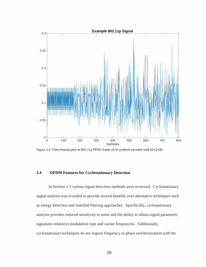
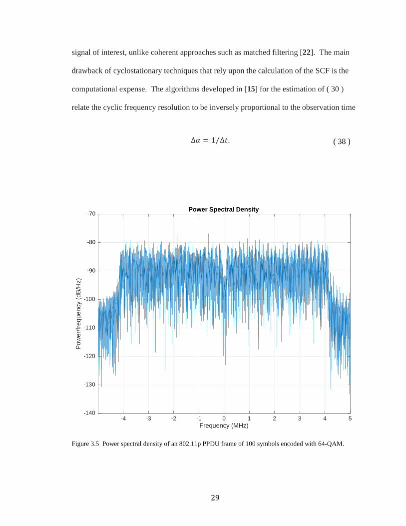
Figure 3.4. An example power spectral density of a signal with 100 symbols encoded
with m=6 is shown in Figure 3.5.
28
Figure 3.4 Time-domain plot an 802.11p PPDU frame of 10 symbols encoded with 64-QAM.
3.4 OFDM Features for Cyclostationary Detection
In Section 1.3 various signal detection methods were reviewed. Cyclostationary
signal analysis was revealed to provide several benefits over alternative techniques such
as energy detection and matched filtering approaches. Specifically, cyclostationary
analysis provides reduced sensitivity to noise and the ability to obtain signal parametric
signatures related to modulation type and carrier frequencies. Additionally,
cyclostationary techniques do not require frequency or phase synchronization with the
0 100 200 300 400 500 600 700 800Samples
0
0.05
0.1
0.15
0.2
0.25
0.3Example 802.11p Signal
29
signal of interest, unlike coherent approaches such as matched filtering [22]. The main
drawback of cyclostationary techniques that rely upon the calculation of the SCF is the
computational expense. The algorithms developed in [15] for the estimation of ( 30 )
relate the cyclic frequency resolution to be inversely proportional to the observation time
∆? = 1 ∆9⁄ . ( 38 )
Figure 3.5 Power spectral density of an 802.11p PPDU frame of 100 symbols encoded with 64-QAM.
-4 -3 -2 -1 0 1 2 3 4 5Frequency (MHz)
-140
-130
-120
-110
-100
-90
-80
-70
Pow
er/fr
eque
ncy
(dB
/Hz)
Power Spectral Density
30
The reliability of the SCF approximations to adequately resolve spectral and
cyclic frequency elements of the signal of interest can thus impose a heavy computational
burden as well as slow down the detection time by requiring longer observation periods.
However, if the signal of interest is known apriori, then the SCF can reveal cyclic
signatures that could be utilized in the detection of the signal. Consequently, provided
the cyclic signatures are unique, the computation of the SCF may be avoided in favor of
the computationally inexpensive calculation of the CAF that corresponds to specific lag
values and cyclic frequencies of the related signatures. Therefore, using the model
described in the previous section, the SCF is generated for an example 802.11p frame,
shown in Figure 3.6. The related contour is shown in Figure 3.7.
3.4.1 Preamble
Perhaps the most obvious signal signature of an 802.11p frame that is useful for
detection is the PPDU preamble consisting of short and long training sequences. These
sequences are located at known subcarriers with known amplitude and phase, as given in
( 36 ) and ( 37 ). In fact, one of the intended functions of the preamble sequences is
identification by a corresponding 802.11p device for clear channel assessment prior to
transmission as well as incoming signal detection. However, the main drawback of the
preamble sequence is its relatively infrequent occurrence. The preamble sequence occurs
only at the beginning of a PPDU frame transmission. The number of symbols, ����, in a
PPDU frame is given by [21]
���� = ��16 + 8 ∙ ������ + 6� ��rv�⁄ �. ( 39 )

31
Figure 3.6 Estimated spectral correlation density of an 802.11p PPDU frame.
Because the byte length of a PPDU frame may be up to 4095 bytes according to the 12-
bit LENGTH subfield, the probability of detection of an 802.11p transmitter using only
the 12 symbols of the preamble sequence is less than 1% in the worst case scenario where
the modulation type is ½ rate BPSK with a data bits per symbol, ��rv�, of 24. Such a
detection mechanism by a secondary user would be susceptible to assuming an
unoccupied channel when in fact a primary user may indeed be transmitting. Extended
sensing time prior to transmission would be required in order to mitigate the possibility of
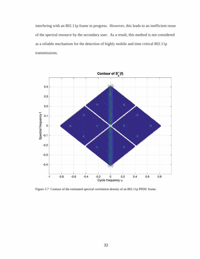
32
interfering with an 802.11p frame in progress. However, this leads to an inefficient reuse
of the spectral resource by the secondary user. As a result, this method is not considered
as a reliable mechanism for the detection of highly mobile and time critical 802.11p
transmissions.
Figure 3.7 Contour of the estimated spectral correlation density of an 802.11p PPDU frame.
33
3.4.2 Pilots
Each OFDM symbol dedicates four subcarriers for use as pilot signals. These
signals are utilized by an 802.11p receiver in order to provide robustness against
frequency offsets and phase noise [21]. They are received coherently with the rest of the
symbol and used by the receiver for frequency correction and equalization. The pilot
subcarriers are modulated by a pseudo-random binary sequence to prevent the generation
of spectral lines. However, each subcarrier is modulated by the same value in the
pseudo-random binary sequence, creating the opportunity for cyclic detection. Moreover,
the pseudo-random sequence is only 127 elements long, after which the sequence repeats
[21]. For PPDU frames that exceed 127 OFDM symbols, this repetition should also
provide a means for cyclic detection. Indeed, careful examination of Figure 3.7 reveals
the presence of cyclic features that correspond to the pilot symbols located at subcarriers
±7, ±21. These cyclic features can be more clearly revealed by modifying the model to
replace the pilot subcarriers with null subcarriers. This exposes the pilot subcarriers in a
similar pattern to the null subcarrier located at DC and is shown in Figure 3.8. Between
Figure 3.7 and Figure 3.8, it can be observed that spectral lines are produced at the cyclic
intersections of the pilot subcarriers, which are given by the coordinates
? = ±�L�O − L�Q� ∙ ∆AA = ±�L�O + L�Q� ∙ ∆A 2⁄ , ( 40 )
where
L�O, L�Q = �±7,±21�L�O ≠ L�Q�. ( 41 )
34
These intersections represent the correlation of the identical pilot subcarriers in a
symbol at the various cyclic and spectral frequencies listed in ( 40 ), as well as the
correlation from the contribution of the pilot subcarriers to the symbol’s cyclic prefix. To
illustrate this point, the simulation model is modified again to provide random
modulation values for each pilot subcarrier, which eliminates their cyclic features in the
SCD as shown in Figure 3.9.
Figure 3.8 Contour of the estimated spectral correlation density of an 802.11p PPDU frame modified by replacing the pilot subcarriers with nulls.
35
Clearly the pilot subcarriers could be utilized as a means of detection of a primary
802.11p signal due to their cyclostationary signature. However, the pilots are spread over
a relatively wide bandwidth, which is subject to dispersion. In fact, the pilots are
intended to be used by an 802.11p receiver in order to provide channel estimation and
frequency equalization. In poor channel conditions the pilots will begin to become
uncorrelated, thus weakening their cyclic features. Additionally, the cyclic features
produced by the pilots exist at relatively narrow spectral frequencies and occur at
multiple cyclic frequencies, which complicates their detection. Therefore, the pilot
subcarriers are deemed as a possible, but not desired, element to use for primary signal
detection.
Figure 3.9 Contour of the estimated spectral correlation density of an 802.11p PPDU frame modified by randomizing the pilot subcarriers.
36
3.4.3 Cyclic Prefix
A cyclic prefix is utilized in OFDM systems, including 802.11p, in order to
combat the effects of multipath fading. In 802.11p the cyclic prefix consists of the last 16
samples of the time-domain symbol being replicated at the front of the symbol. This
predictable repetition should generate spectral lines in a cyclostationary analysis, and in
fact they are revealed in the contour shown in Figure 3.7 as the multiple spectral lines
close to ? = 0. Figure 3.10 shows the cycle frequency cross-section of Figure 3.6 to
more clearly display these spectral lines.
The source of these spectral lines can be determined analytically. Consider that
the complex envelop of an OFDM symbol with subcarriers modulated with QAM
sequences can be represented by [23]
8�9� = � � ��,�cd e�f ^��l⁄ ��9 − D��������l������ ( 42 )
where ��,� is an independent and identically distributed message sequence representing
the symbol QAM data, ��9� is a square shaping pulse with duration���� = �&&^ + ���, and �&&^ is the number of subcarriers. The spectral correlation function of the complex
envelope of 8�9� is then given as [23]
LOZ�A� =����� �� ���� � 0,A − ��&&^ + ?2/ ∙ 0∗ ,A − ��&&^ − ?2/ ,
���l����� ? = ����
0, ? ≠ ���� ( 43 )
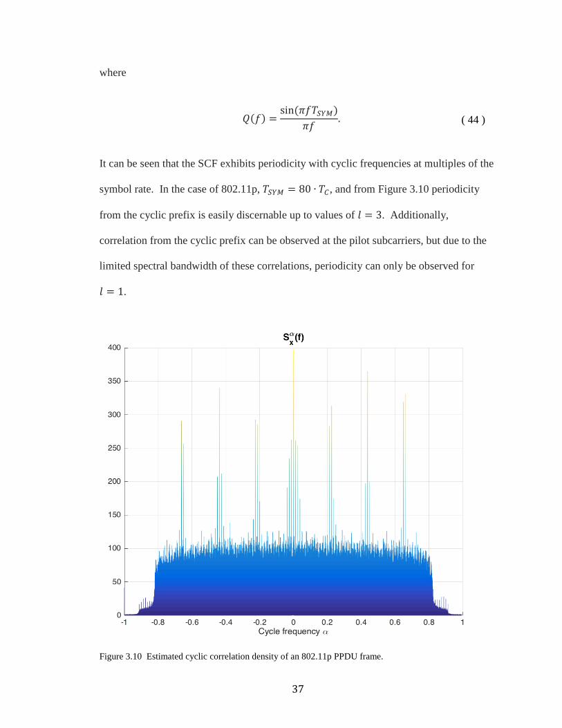
37
where
0�A� = sin�>A�����>A . ( 44 )
It can be seen that the SCF exhibits periodicity with cyclic frequencies at multiples of the
symbol rate. In the case of 802.11p, ���� = 80 ∙ �¢, and from Figure 3.10 periodicity
from the cyclic prefix is easily discernable up to values of = 3. Additionally,
correlation from the cyclic prefix can be observed at the pilot subcarriers, but due to the
limited spectral bandwidth of these correlations, periodicity can only be observed for
= 1.
Figure 3.10 Estimated cyclic correlation density of an 802.11p PPDU frame.
38
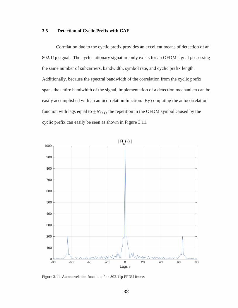
3.5 Detection of Cyclic Prefix with CAF
Correlation due to the cyclic prefix provides an excellent means of detection of an
802.11p signal. The cyclostationary signature only exists for an OFDM signal possessing
the same number of subcarriers, bandwidth, symbol rate, and cyclic prefix length.
Additionally, because the spectral bandwidth of the correlation from the cyclic prefix
spans the entire bandwidth of the signal, implementation of a detection mechanism can be
easily accomplished with an autocorrelation function. By computing the autocorrelation
function with lags equal to ±�&&^, the repetition in the OFDM symbol caused by the
cyclic prefix can easily be seen as shown in Figure 3.11.
Figure 3.11 Autocorrelation function of an 802.11p PPDU frame.
39
The cyclic autocorrelation function (CAF) described by ( 18 ) can then be applied,
assuming a signal at the baseband sampling rate, for fixed lag values U = ±�&&^ at cyclic
frequencies corresponding to the total symbol sample length ? = 1 ��&&^ + ����⁄ , where
��� indicates the number of baseband samples in the guard interval. The discrete
estimation of the CAF over � samples is given by
W¤OZ�U� = � 8[�]8∗[� + U]c�d eZ������� ( 45 )
which is the sum of the CAF and an error term ¥OZ�U� W¤OZ�U� = WOZ�U� + ¥OZ�U�. ( 46 )
It is desired to form a test to determine the presence of the primary signal based on the
computation of the CAF, therefore a test hypothesis is formulated similar to ( 3 )
ℋ� : ¦O = §Oℋ� : ¦O = ¦© + §O,
( 47 )
where
¦O = {Re�W¤OZ�U���,… ,Re�W¤OZ�U���,Im�W¤OZ�U���,… ,Im�W¤OZ�U���| ( 48 )
and
§O = [Re"¥OZ�U��%,… ,Re"¥OZ�U��%,Im"¥OZ�U��%,… ,Im"¥OZ�U��%]. ( 49 )
40
For the scenario where D = 2, if the samples 8[�] that are well separated in time
are approximately independent [24], then it can be shown that the error vector has a
multivariate normal distribution with zero mean and noise covariance matrix ®, i.e.
lim�→H√�§O ~+�¯, ®�. ( 50 )
The test statistic is then defined as
��¦O� = � ∙ ¦O®��¦OT , ( 51 )
which under the null hypothesis is chi-square distributed with 2D degrees of freedom
��¦O�|ℋ�~° � . ( 52 )
A threshold value can be set in order to provide a constant false alarm rate
�&' = �� !"��¦O� > �|ℋ�%, ( 53 )
which the distribution given by ( 52 ) allows to be calculated as
� = ±²³´³�� �1 − �&'�, ( 54 )
where ±²³´³�� is the inverse cumulative distribution function of ° � [24].
Similar to the example energy based detector example given in Section 1.3.1, in
order to implement a test for cyclostationarity using the CAF the covariance matrix must
be estimated from the received signal and its inversion calculated [25]. In Chapter 4, a
technique that eliminates the need to estimate and invert the covariance matrix will be
introduced.

41
CHAPTER 4
DSRC DETECTION WITH CAF
4.1 Spatial Sign Cyclic Correlation Estimator
The previous chapter reviewed various OFDM signal features for potential use in
a cyclostationary detection scheme. The cyclic prefix was found to introduce strong
cyclostationary effects making it an ideal candidate for the detection of 802.11p primary
users. Moreover, the CAF provides a computationally efficient means by which to
calculate the cyclostationary properties of the cyclic prefix. Unfortunately, the detection
method requires estimation and inversion of the signal noise covariance matrix. In real
applications the noise statistics may not be known completely, in which case an SNR
wall develops in the detection scheme as discussed in Section 1.3.1. Additionally, any
statistics estimation is subject to frequent change due to the mobile environment in which
802.11p exists. It is therefore desired to develop a detection mechanism that does not
require computation of the noise statistics.
One such method proposed in [26] utilizes the spatial sign function (SSF) in order
to avoid estimation of the noise probability density function. The SSF for a complex
input signal 8[�] is given as
L�8[�]� = µ 8[�]|8[�]| 8[�] ≠ 00 8[�] = 0 ( 55 )
The SSF is a nonlinear operation that normalizes the input signal to exist on the unit
circle in the complex plane, with the key assumption that the data possesses zero mean.
42
If the mean is not zero, it should be estimated and removed. The spatial sign cyclic
correlation estimator (SSCCE) is then given as
W¤¶Z�U� = 1�� L�8[�]�L�8∗[� + U]�c�d eZ�, ∀U������ ≠ 0 ( 56 )
In [26] it is shown that the nonlinearity of the SSF does not affect the periodicity of the
autocorrelation function for circularly symmetric complex Gaussian processes (an
accurate model for OFDM systems).
As before, a test statistic is defined to reject the null hypothesis that the received
signal does not contain the primary signals. In order to compute the test statistic, it is
first necessary to determine the distribution of the SSCCE for an i.i.d. circular noise
process with zero mean, �[�]. The mean of the SSCCE for �[�] is thus [26]
Ε{W¤¶Z�U�| = 1�� Ε[L��[�]�L��∗[� + U]�]c�d eZ����
���= 1�� Ε[L��[�]�]Ε[L��∗[� + U]�]c�d eZ� = 0, ∀?���
��� ( 57 )
The covariance of the SSCCE for �[�] is given by
® ¤¹º�i� = Ε{W¤¶Z�U�W¤¶Z∗�U�|= Ε »¼1�� L��[�]�L��∗[� + U]�c�d eZ����
��� ½ ∙¼1�� L��[�]�L��∗[� + U]�c�d eZ����
��� ½∗¾= 1� �Ε[|L��[�]�| |L��[� + U]�| ]���
��� . ( 58 )
43
The normalization property of the SSF ensures that
Ε[|L��[�]�| |L��[� + U]�| ] = 1 ( 59 )
Therefore the covariance of the noise process after normalization from the SSF is
® ¤¹º�i� = 1� IIII. ( 60 )
A test hypothesis is again formulated
ℋ� : 8[�] = �[�]ℋ� : 8[�] = �[�] + �[�], ( 61 )
where �[�] is the primary signal of interest. A vector of the calculated SSCCE functions
for various lag values is given as
¦¶ = {W¤¶Z�U��,… , W¤¶Z�U��|. ( 62 )
From ( 60 ) it follows that ¦¶ is complex normal distributed
lim�→H¦¶|ℋ� ~¿+ ,¯, 1� IIII/. ( 63 )
Then the test statistic can be given as [26]
��¦¶� = � ∙ ‖¦¶‖ , ( 64 )

44
which under the null hypothesis is chi-square distributed with D complex degrees of
freedom
��¦¶�|ℋ� ~°� . ( 65 )
The threshold is then calculated according to the desired false alarm rate
� = ±����1 − �&'�, ( 66 )
where ±��� is the inverse gamma cumulative distribution function with scale factor of one
and shape factor D [25].
4.2 Dual-Lag SSCCE with Cyclic Phase Compensation
As discussed in Section 3.4.3, the cyclic prefix induces strong cyclostationary
features that can be detected with the CAF. As illustrated in Figure 3.11, correlation
occurs at lags ±�&&^, which is 64 in the case of 802.11p and clearly visible in Figure
3.10 for cyclic frequencies ? = ��&&^ + ����⁄ , = 0,±1,±2, ±3. The detection
scheme proposed is to calculate the SSCCE at dual lags U = ±64 and ? = 1 80⁄ . The
test statistic from ( 64 ) is then
��¦¶� = � ∙ �W¤¶Z�U��� + � ∙ �W¤¶Z�U �� . ( 67 )
In [27] it is shown that for a dual-lag (D = 2) with cyclic frequency ? =1 ��&&^ + ����⁄ , a cyclic phase compensation can be introduced in order to align the

45
SSCCE values of the two lags in time. The two SSCCE computations are complex
valued and have an instantaneous phase difference
∅ = arg�W¤¶Z�U��� + arg�W¤¶Z�U ��. ( 68 )
For an 802.11p primary signal that exhibits correlation at the lag values from the cyclic
prefix, the phase difference ∅ is a constant value based on U and ? [27]
∅ = 2πτ�α. ( 69 )
The constant phase difference correction is applied to the second SSCCE calculation
W¤¶Z∅�U � = 1�� L�8[�]�L�8∗[� + U ]�c�d eZ�o∅.������ ( 70 )
Because the two SSCCEs are now coherent the test statistic can be summed simply as
��¦¶N� = �2 ∙ tW¤¶Z�U�� + W¤¶Z∅�U �t ,
( 71 )
which lowers the degrees of freedom to D = 1 as well as reduces the implementation
complexity. The threshold value is computed the same as ( 66 ) but with scale and shape
factors of one.
4.3 MATLAB Simulation
The previous section detailed a cyclostationary detection method based on the
CAF that avoids the necessity of estimating the noise covariance by normalizing the

46
signal via the SSF. In order to test the performance and suitability of this method for
hardware implementation, a MATLAB simulation was developed. The 802.11p
baseband simulation model described in Section 3.3 was used to generate various size
PPDU frames. The baseband data was subjected to several impairments to simulate real
world channel effects. First, multipath fading was simulated via a Rayleigh model with
Doppler shift corresponding to a mobile unit velocity of 130kph. Additionally, the
baseband data was shifted 30kHz in order to model a local oscillator offset of 5ppm,
which is representative of the maximum typical offset error [28]. Finally, measured
additive white Gaussian noise was added to the baseband signal to further simulate the
channel. The SSCCE algorithm with cyclic phase compensation, ( 70 ), was coded as a
MATLAB function, sscce_pc.m, and is included in Appendix A. The function is
parameterized by x the baseband input signal, alpha the cyclic frequency, phi the cyclic
phase compensation (vector valued), and lag the desired lags for the autocorrelation (also
vector valued). The signal test statistic is calculated from the SSCCE function for
U = ±64 and ? = 1 80⁄ , which is returned along with the calculated SSCCE values. The
threshold value is set according to ( 66 ) for a standard false alarm probability of 5%.
4.3.1 Probability of Detection vs. SNR
Because the detection scheme operates by correlating N samples, the probability
of detection will increase with larger input signal length. However, to simulate realistic
scenarios, typical message lengths should be used. The DSRC describes over 150 data
elements that can be included in a DSRC message [29]. The data elements describe such
information as vehicle acceleration, speed, heading, anti-lock brake status, wiper status,
47
etc. From these elements, eight high-priority safety messages have been defined. Since
these messages are the ones for which detection is paramount, the simulated 802.11p
frame should be representative of a typical safety message length. After encoding and
protocol encapsulation of the per message data elements, a high-priority safety message
may be comprised of approximately 856 to 1408 bits at the PHY PSDU [29]. Depending
on the subcarrier modulation scheme, according to ( 39 ) the corresponding number of
symbols for the smallest safety message encoded at the highest data rate of 27 Mbps is 33
symbols, which represents the worst case signal detection scenario.
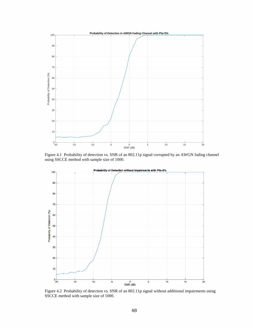
Simulations were performed in order to test reliability and performance of the
SSCCE detector in varied noise environments. A baseband 802.11p signal 33 symbols in
length was generated with the impairments described in the previous section along with
measured amounts of AWGN. The SSCCE output test statistic was compared against the
threshold value computed for 5% false alarm rate and plotted versus signal SNR, as
shown in Figure 4.1. The test was run with a sample size of 1000. As expected, the
detection rate trends towards 5% as the noise level increases. Also, observe that despite
the relatively few samples used for the correlation (2640 baseband samples), the
probability of detection is effectively 100% for any SNR greater than 5dB. The same
simulation repeated but without multipath fading or LO offset impairments is shown in
Figure 4.2, which indicates approximately 5dB improvement over the previous scenario.
48
Figure 4.1 Probability of detection vs. SNR of an 802.11p signal corrupted by an AWGN fading channel using SSCCE method with sample size of 1000.
Figure 4.2 Probability of detection vs. SNR of an 802.11p signal without additional impairments using SSCCE method with sample size of 1000.
-20 -15 -10 -5 0 5 10 15 20SNR (dB)
0
10
20
30
40
50
60
70
80
90
100
Pro
babi
lity
of D
etec
tion
(%)
Probability of Detection in AWGN Fading Channel with Pfa=5%
49
4.3.2 ROC at Fixed SNR
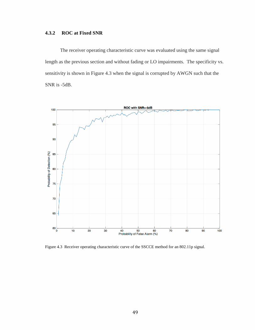
The receiver operating characteristic curve was evaluated using the same signal
length as the previous section and without fading or LO impairments. The specificity vs.
sensitivity is shown in Figure 4.3 when the signal is corrupted by AWGN such that the
SNR is -5dB.
Figure 4.3 Receiver operating characteristic curve of the SSCCE method for an 802.11p signal.
50
4.3.3 Histogram at Fixed SNR
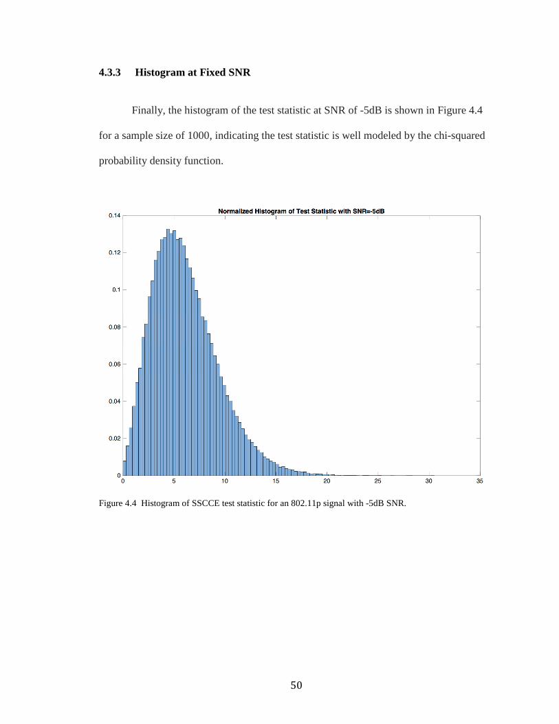
Finally, the histogram of the test statistic at SNR of -5dB is shown in Figure 4.4
for a sample size of 1000, indicating the test statistic is well modeled by the chi-squared
probability density function.
Figure 4.4 Histogram of SSCCE test statistic for an 802.11p signal with -5dB SNR.
51
CHAPTER 5
FPGA IMPLEMENTATION
5.1 FPGA Overview
As discussed in Section 1.2, spectrum sharing in the DSRC band has several
unique challenges. First, the detection methodology must be robust. Several detection
schemes have been discussed in the previous chapters. Of those discussed, a
cyclostationary method for the detection of the OFDM symbol’s cyclic prefix appears to
be the most promising for robustness against noise and probability of detection.
Secondly, the detection method must provide rapid discovery of primary users. The
SSCCE approach reviewed in Chapter 4 was shown to provide detection of 802.11p
signals within a fixed number of baseband samples corresponding to a shortest case
DSRC safety message. Furthermore, the SSCCE method is not computationally taxing,
which addresses the final constraints for a DSRC spectrum-sharing device, namely that it
be power and resource efficient. It is expected that a detection engine for 802.11p signals
would be implemented in a radio chipset to achieve real-time and power efficient
operation. This chapter will review a field programmable gate array (FPGA)
implementation of the SSCCE algorithm discussed in Chapter 4.
FPGAs are programmable digital logic devices that contain various logic gates
(NOT, OR, AND, XOR, etc.) along with flip-flops and configurable routing
interconnects. The logic elements can be programmed after manufacture to implement
arbitrary and complex digital logic functionality. A hardware description language
(HDL) is used to define the design functionality, typically either Verilog or VHDL.
52
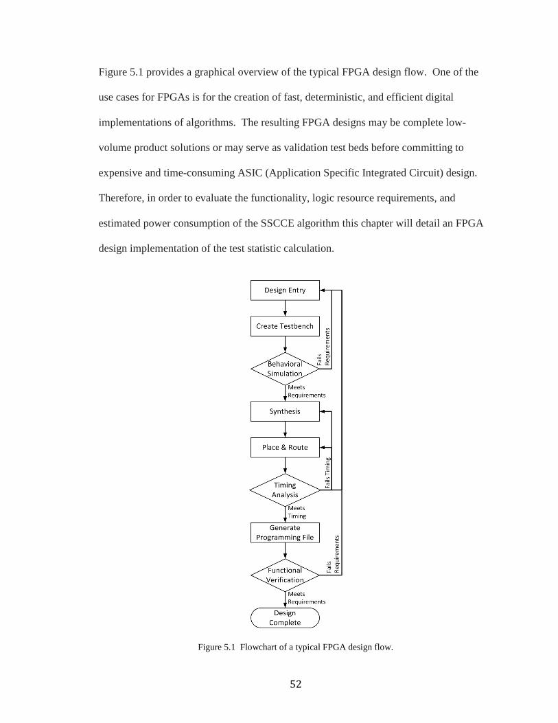
Figure 5.1 provides a graphical overview of the typical FPGA design flow. One of the
use cases for FPGAs is for the creation of fast, deterministic, and efficient digital
implementations of algorithms. The resulting FPGA designs may be complete low-
volume product solutions or may serve as validation test beds before committing to
expensive and time-consuming ASIC (Application Specific Integrated Circuit) design.
Therefore, in order to evaluate the functionality, logic resource requirements, and
estimated power consumption of the SSCCE algorithm this chapter will detail an FPGA
design implementation of the test statistic calculation.
Figure 5.1 Flowchart of a typical FPGA design flow.

53
5.2 SSCCE Algorithm Implementation
The SSCCE algorithm was broken into several design elements to simplify
development into smaller, more easily verified blocks, which also increases design
reusability. The design was coded in VHDL, whereas the behavioral testbench was
coded in SystemVerilog. All design blocks were coded in pure HDL in order to make
use of synthesis inference as opposed to using vendor intellectual property design cores
that limit portability. The design was divided into the following blocks: SSF, lead/lag
shift register, complex multiplier for the correlation coefficient, numerically controlled
oscillator and complex multiplier for the cyclic down conversion of the correlation
coefficients, moving average, real multiplier, and adders, all as indicated in Figure 5.2.
The top-level design file is given in Appendix B as sscce.vhd.
Figure 5.2 Block diagram of the FPGA implementation of the SSCCE algorithm.

54
5.2.1 Spatial Sign Function
The SSF computes the unit vector of the input signal. Normally, this involves the
calculation
L�8[�]� = ÈRe�8[�]� + Im�8[�]� . ( 72 )
However, this method is expensive in digital logic due to the multiplication required for
the two square terms and especially the square-root function. One method to avoid both
operations is to obtain the phase angle of the Cartesian input signal and then convert the
angle to Cartesian coordinates assuming a normalized magnitude
@ = tan ,Im�8�Re�8�/L�8� = cos�@� + � sin�@�.
( 73 )
The transcendental functions required in ( 73 ) would appear to be more troublesome than
the square-root function in ( 72 ), however very efficient methods exist for their
calculation in digital hardware. The Coordinate Rotational Digital Computer (CORDIC)
algorithm calculates trigonometric functions iteratively using only additions and bit shift
operations [30].
Two general modes of the algorithm exist. The vectoring mode accepts a
Cartesian input signal and through a series of additions and shifts rotates the vector to lie
on the real axis. The rotation angle that was required to rotate the vector onto the real
axis is the resulting phase angle and the real component of the rotated vector is
proportional to the vector magnitude. The other mode of operation is known as the
55
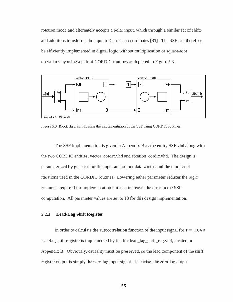
rotation mode and alternately accepts a polar input, which through a similar set of shifts
and additions transforms the input to Cartesian coordinates [31]. The SSF can therefore
be efficiently implemented in digital logic without multiplication or square-root
operations by using a pair of CORDIC routines as depicted in Figure 5.3.
Figure 5.3 Block diagram showing the implementation of the SSF using CORDIC routines.
The SSF implementation is given in Appendix B as the entity SSF.vhd along with
the two CORDIC entities, vector_cordic.vhd and rotation_cordic.vhd. The design is
parameterized by generics for the input and output data widths and the number of
iterations used in the CORDIC routines. Lowering either parameter reduces the logic
resources required for implementation but also increases the error in the SSF
computation. All parameter values are set to 18 for this design implementation.
5.2.2 Lead/Lag Shift Register
In order to calculate the autocorrelation function of the input signal for U = ±64 a
lead/lag shift register is implemented by the file lead_lag_shift_reg.vhd, located in
Appendix B. Obviously, causality must be preserved, so the lead component of the shift
register output is simply the zero-lag input signal. Likewise, the zero-lag output
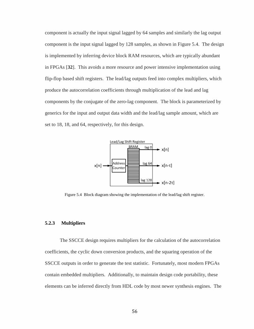
56
component is actually the input signal lagged by 64 samples and similarly the lag output
component is the input signal lagged by 128 samples, as shown in Figure 5.4. The design
is implemented by inferring device block RAM resources, which are typically abundant
in FPGAs [32]. This avoids a more resource and power intensive implementation using
flip-flop based shift registers. The lead/lag outputs feed into complex multipliers, which
produce the autocorrelation coefficients through multiplication of the lead and lag
components by the conjugate of the zero-lag component. The block is parameterized by
generics for the input and output data width and the lead/lag sample amount, which are
set to 18, 18, and 64, respectively, for this design.
Figure 5.4 Block diagram showing the implementation of the lead/lag shift register.
5.2.3 Multipliers
The SSCCE design requires multipliers for the calculation of the autocorrelation
coefficients, the cyclic down conversion products, and the squaring operation of the
SSCCE outputs in order to generate the test statistic. Fortunately, most modern FPGAs
contain embedded multipliers. Additionally, to maintain design code portability, these
elements can be inferred directly from HDL code by most newer synthesis engines. The

57
autocorrelation and cyclic down conversion operations have complex inputs and therefore
require complex multipliers. The complex multiplier design actually consists of four
individual multiplication operations along with addition and subtraction of the four
products to provide the complex output. The design implementation is provided in
Appendix B as complex_mult.vhd. Likewise, the squaring operation used in the
formation of the test statistic has purely real or purely imaginary inputs and so only
requires a real multiplication, which is also given in Appendix B as real_mult.vhd.
Binary multiplications create an output bit width of twice the input bit width. However,
it is often desired to maintain a constant bus width between processing elements.
Therefore, the above designs are parameterized by a generic that scales the output by a
desired factor-of-two to help maintain numerical precision of the multiplication output
when its length is reduced to the input width. This scaling factor needs to be accounted
for in the final output. When the multiplier output signal length is reduced, the least
significant bits can be rounded off or simply truncated. Rounding reduces error but
increases device resource utilization. This design uses a data width of 18 bits for all
multipliers, which matches the typical multiplier width common to most FPGA
manufacturers. Through empirical testing, rounding was not shown to improve the
accuracy of the test statistic and so was disabled to reduce resource requirements.
5.2.4 Numerically Controlled Oscillator
The calculation of the cyclic down conversion of the autocorrelation coefficients
requires a multiplication by a pair of complex exponentials that are offset by a constant
phase shift. There are several common methods to generate a complex exponential in
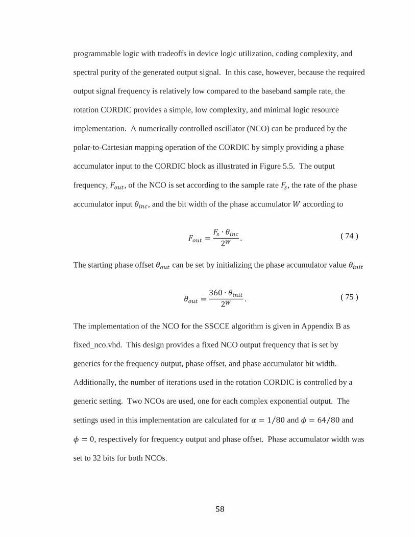
58
programmable logic with tradeoffs in device logic utilization, coding complexity, and
spectral purity of the generated output signal. In this case, however, because the required
output signal frequency is relatively low compared to the baseband sample rate, the
rotation CORDIC provides a simple, low complexity, and minimal logic resource
implementation. A numerically controlled oscillator (NCO) can be produced by the
polar-to-Cartesian mapping operation of the CORDIC by simply providing a phase
accumulator input to the CORDIC block as illustrated in Figure 5.5. The output
frequency, ±�nf, of the NCO is set according to the sample rate ±¶, the rate of the phase
accumulator input @�N, and the bit width of the phase accumulator � according to
±�nf = ±¶ ∙ @Ê�N2Ë . ( 74 )
The starting phase offset @�nf can be set by initializing the phase accumulator value @Ê�Êf @�nf = 360 ∙ @Ê�Êf2Ë . ( 75 )
The implementation of the NCO for the SSCCE algorithm is given in Appendix B as
fixed_nco.vhd. This design provides a fixed NCO output frequency that is set by
generics for the frequency output, phase offset, and phase accumulator bit width.
Additionally, the number of iterations used in the rotation CORDIC is controlled by a
generic setting. Two NCOs are used, one for each complex exponential output. The
settings used in this implementation are calculated for ? = 1 80⁄ and Ì = 64 80⁄ and
Ì = 0, respectively for frequency output and phase offset. Phase accumulator width was
set to 32 bits for both NCOs.
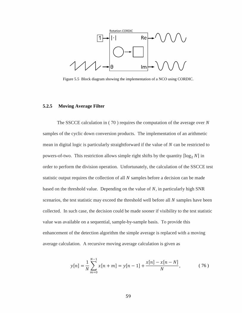
59
Figure 5.5 Block diagram showing the implementation of a NCO using CORDIC.
5.2.5 Moving Average Filter
The SSCCE calculation in ( 70 ) requires the computation of the average over �
samples of the cyclic down conversion products. The implementation of an arithmetic
mean in digital logic is particularly straightforward if the value of � can be restricted to
powers-of-two. This restriction allows simple right shifts by the quantity �log �� in
order to perform the division operation. Unfortunately, the calculation of the SSCCE test
statistic output requires the collection of all � samples before a decision can be made
based on the threshold value. Depending on the value of �, in particularly high SNR
scenarios, the test statistic may exceed the threshold well before all � samples have been
collected. In such case, the decision could be made sooner if visibility to the test statistic
value was available on a sequential, sample-by-sample basis. To provide this
enhancement of the detection algorithm the simple average is replaced with a moving
average calculation. A recursive moving average calculation is given as
�[�] = 1� � 8[� + Í] = �[� − 1] + 8[�] − 8[� − �]����Î�� , ( 76 )

60
which is easily implemented in digital logic (again with the caveat that � is restricted to
powers-of-two), but requires additional block RAM resources that are otherwise not
necessary in a simple arithmetic mean. However, the ability to provide immediate
detection of a primary user before the collection of all � samples is considered a
favorable tradeoff against increased logic utilization. The moving average design
implementation is located in Appendix B as moving_average.vhd. The design is
parameterized by a generic to set the maximum number of samples in the calculation.
The size of the moving average can be adjusted during runtime up to the maximum value
specified. The design implementation for the SSCCE sets the maximum number of
samples to 2048. Binary addition grows the summand by one bit for every addition
operation performed. Similar to the multiplier implementations, it is often desirable to
maintain the output signal width to match the input signal width with an implied scaling
applied to the output signal following truncation. A generic parameter is available to
maintain bit precision of the output by shifting the output by a power-of-two. Through
empirical examination of the output signal, the scaling parameter of four was determined
to provide enhanced bit precision while preventing numerical overflow. This scales the
output by an additional factor of 16. The design was implemented such that the sample
memory infers device block RAM resources for efficient implementation [32].
5.3 SSCCE Behavioral Simulation
Following design implementation in HDL the next step is to verify the coded
operation meets design expectations. This is typically done using a design behavioral
simulation. There are a variety of methodologies in practice to perform behavioral

61
simulation, but the general model is to create a separate entity referred to as a testbench,
which feeds stimulus to the design under test (DUT) and captures the resulting response.
The response is compared against the expected results for a given stimulus to detect
design errors. Often it is desirable to test using some form of constrained random
stimulus in order to attempt to test various corner cases in the design implementation.
The testbench and DUT are simulated using an HDL simulator that allows per cycle
analysis and debug of the various design elements.
For this design, Mentor Graphics® Questa Sim was used along with a testbench
written in SystemVerilog. A screenshot of the simulator with several of the sscce.vhd
signals plotted is shown in Figure 5.6. The test methodology of the SSCCE design
implementation is as follows. First, the MATLAB functions used for the generation of
the 802.11p baseband signal were reused, including the multipath fading and LO
frequency offset impairments. Sixteen thousand random baseband signals were
generated with SNR values ranging between -20dB to +10dB. Because the
implementation of the SSCCE function is restricted to average over powers-of-two, the
signal length was reduced from 2640 (as used in Chapter 4 as a shortest-case DSRC
safety message) to 2048 baseband samples. Each stimulus signal was saved individually
in a file as a set of integer values less than the full-scale data width used in the sscce.vhd
design (18 bits). The stimulus files were opened by the testbench simulation and the
baseband signal used as input to the sscce.vhd DUT. The test statistic output signal of the
DUT was likewise captured as a response file for every stimulus file.
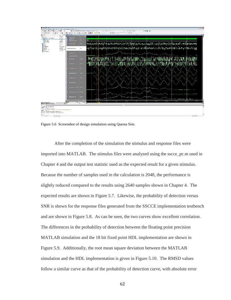
62
Figure 5.6 Screenshot of design simulation using Questa Sim.
After the completion of the simulation the stimulus and response files were
imported into MATLAB. The stimulus files were analyzed using the sscce_pc.m used in
Chapter 4 and the output test statistic used as the expected result for a given stimulus.
Because the number of samples used in the calculation is 2048, the performance is
slightly reduced compared to the results using 2640 samples shown in Chapter 4. The
expected results are shown in Figure 5.7. Likewise, the probability of detection versus
SNR is shown for the response files generated from the SSCCE implementation testbench
and are shown in Figure 5.8. As can be seen, the two curves show excellent correlation.
The differences in the probability of detection between the floating point precision
MATLAB simulation and the 18 bit fixed point HDL implementation are shown in
Figure 5.9. Additionally, the root mean square deviation between the MATLAB
simulation and the HDL implementation is given in Figure 5.10. The RMSD values
follow a similar curve as that of the probability of detection curve, with absolute error
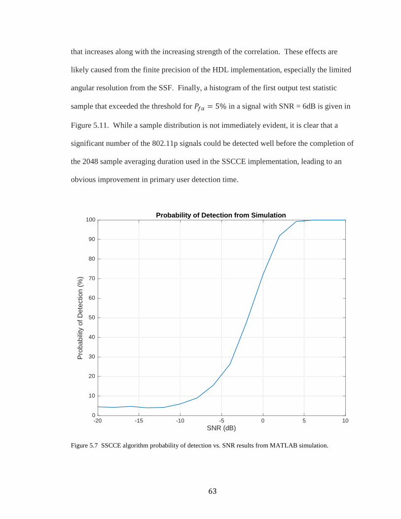
63
that increases along with the increasing strength of the correlation. These effects are
likely caused from the finite precision of the HDL implementation, especially the limited
angular resolution from the SSF. Finally, a histogram of the first output test statistic
sample that exceeded the threshold for �hM = 5% in a signal with SNR = 6dB is given in
Figure 5.11. While a sample distribution is not immediately evident, it is clear that a
significant number of the 802.11p signals could be detected well before the completion of
the 2048 sample averaging duration used in the SSCCE implementation, leading to an
obvious improvement in primary user detection time.
Figure 5.7 SSCCE algorithm probability of detection vs. SNR results from MATLAB simulation.
-20 -15 -10 -5 0 5 10SNR (dB)
0
10
20
30
40
50
60
70
80
90
100
Pro
babi
lity
of D
etec
tion
(%)
Probability of Detection from Simulation
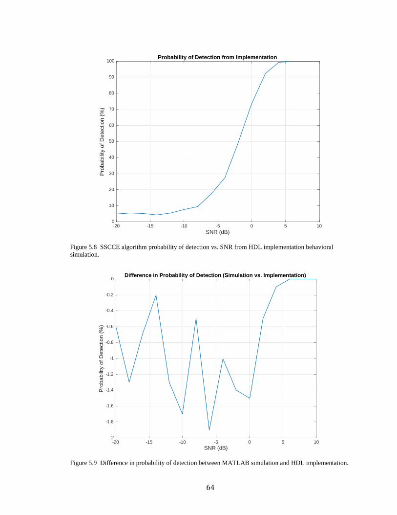
64
Figure 5.8 SSCCE algorithm probability of detection vs. SNR from HDL implementation behavioral simulation.
Figure 5.9 Difference in probability of detection between MATLAB simulation and HDL implementation.
-20 -15 -10 -5 0 5 10SNR (dB)
0
10
20
30
40
50
60
70
80
90
100
Pro
babi
lity
of D
etec
tion
(%)
Probability of Detection from Implementation
-20 -15 -10 -5 0 5 10SNR (dB)
-2
-1.8
-1.6
-1.4
-1.2
-1
-0.8
-0.6
-0.4
-0.2
0
Pro
babi
lity
of D
etec
tion
(%)
Difference in Probability of Detection (Simulation vs. Implementation)
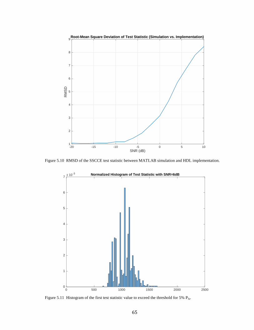
65
Figure 5.10 RMSD of the SSCCE test statistic between MATLAB simulation and HDL implementation.
Figure 5.11 Histogram of the first test statistic value to exceed the threshold for 5% Pfa.
-20 -15 -10 -5 0 5 10SNR (dB)
1
2
3
4
5
6
7
8
9
RM
SD
Root-Mean Square Deviation of Test Statistic (Simulation vs. Implementation)
0 500 1000 1500 2000 25000
1
2
3
4
5
6
7# 10 -3 Normalized Histogram of Test Statistic with SNR=6dB

66
5.4 SSCCE Resource Utilization
Once expected results are obtained from behavioral simulation, the following
steps are to synthesize, place, and route the HDL design. In order to estimate the
necessary design resources and power consumption of the SSCCE design, Altera®
Quartus II software was used. A Cyclone V family device was targeted for
implementation because it represents a modern 28nm, low-power process device
architecture. The results per design block are presented in Table 3. Overall, the resource
utilization is relatively low. The block RAM utilization is the largest resource
requirement by far, which is driven primarily by the moving average blocks.
Table 3 SSCCE Implementation Resource Utilization
Design Block Logic
Elements Flip-Flops Block RAM Bits Multipliers
Dynamic Power Dissipation
SSF 2059 2033 0 0 54mW
Lead/Lag Shift Register
29 57 4608 0 3mW
Complex Multiplier
0 545 0 8 55mW
NCO 2043 2118 0 0 112mW
Moving Average 199 130 118784 0 18mW
Real Multiplier 0 72 0 2 25mW
Misc. 157 53 0 0 61mW
Total 4458 5008 123392 10 328mW

67
5.5 Conclusion
As the demands on the wireless spectrum continue to increase, regulatory
authorities will seek out ways to achieve sharing and reuse of licensed bands. The
techniques being explored in the area of cognitive radio hold promise to help address this
issue. One of the recently proposed areas for spectrum sharing is the DSRC band at 5.9
GHz. The reuse scenario in this band has specific constraints due to the nature of DSRC
communications. Devices wishing to make unlicensed use of the 5.9 GHz band will
require robust and rapid detection of primary users in order to avoid disruption to the
intended operation of DSRC. This thesis explored various cognitive radio detection
methods, including cyclostationary analysis, which was shown to perform well in the
presence of noise. A baseband signal model for 802.11p modulation used by DSRC was
created to explore various features for cyclostationary detection. Several OFDM
modulation features of 802.11p useful for signal identification were discussed. This
thesis investigated a detection method based on the OFDM symbol cyclic prefix. The
cyclic autocorrelation function was introduced as a low computational complexity
method to detect the cyclic prefix. To avoid computation of the signal noise statistics, the
spatial sign function was introduced. The spatial sign cyclic correlation estimator was
then developed in MATLAB and tested with the 802.11p baseband model, showing
encouraging results in the presence of signal impairments for a short duration signal. To
allow real-time execution of the detection algorithm, a digital hardware implementation
was explored by implementing the SSCCE function in HDL. Behavioral simulations
showed good match between the fixed-point hardware implementation and the floating

68
point MATLAB model. Afterwards, resource utilization of the algorithm was estimated
by synthesizing and fitting the design to a FPGA device.
The SSCCE algorithm explored in this thesis appears to be a promising method
for OFDM signal identification, with particular applicability towards spectral reuse in the
DSRC band. The algorithm provides excellent identification of primary users in the
presence of noise and impairments yet has a low computational complexity that provides
for straightforward implementation in digital logic, allowing for low latency, real-time
execution. Further investigation in this area is warranted. A potential area of additional
research includes deployment of the HDL implementation with a RF receiver capable of
operation in the DSRC band in order to test for real world signal environment effects and
performance. Also, the algorithm presented in this thesis operated assuming a baseband
sampling rate. Further research should be performed to identify the effects of sampling
beyond the baseband rate, including non-integer multiples of the baseband rate.
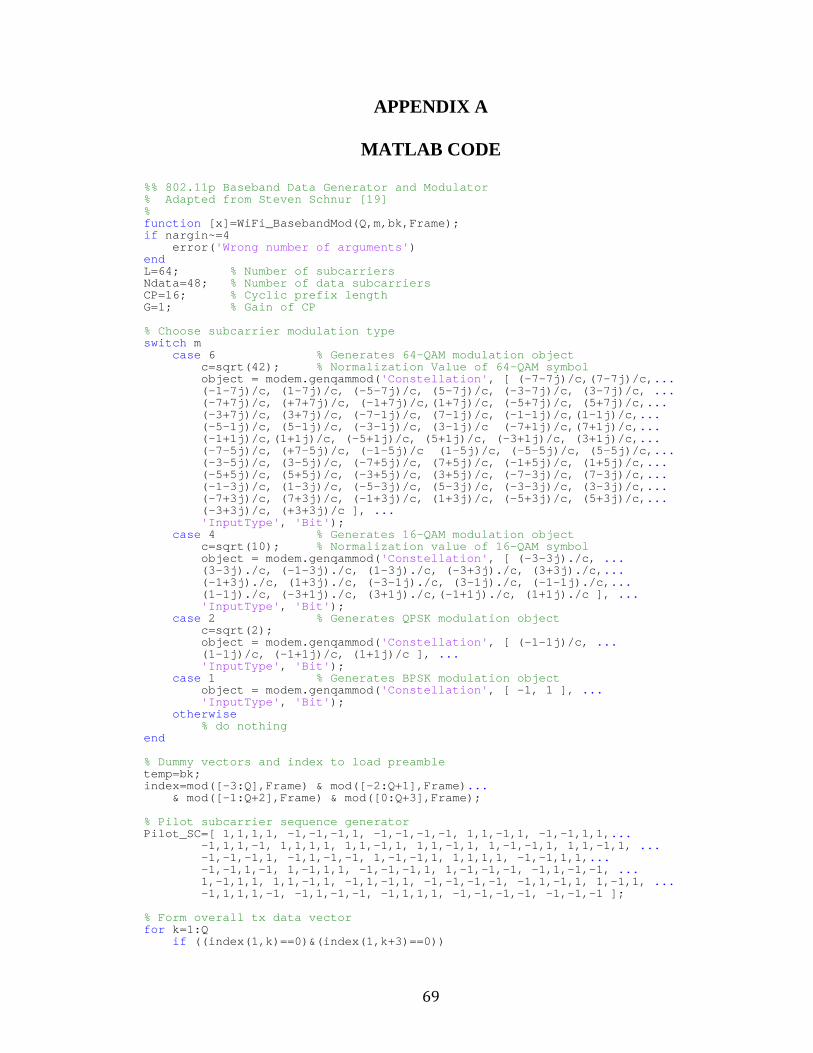
69
APPENDIX A
MATLAB CODE
%% 802.11p Baseband Data Generator and Modulator % Adapted from Steven Schnur [19] % function [x]=WiFi_BasebandMod(Q,m,bk,Frame); if nargin~=4 error( 'Wrong number of arguments' ) end L=64; % Number of subcarriers Ndata=48; % Number of data subcarriers CP=16; % Cyclic prefix length G=1; % Gain of CP % Choose subcarrier modulation type switch m case 6 % Generates 64-QAM modulation object c=sqrt(42); % Normalization Value of 64-QAM symbol object = modem.genqammod( 'Constellation' , [ (-7-7j)/c,(7-7j)/c, ... (-1-7j)/c, (1-7j)/c, (-5-7j)/c, (5-7j)/c, ( -3-7j)/c, (3-7j)/c, ... (-7+7j)/c, (+7+7j)/c, (-1+7j)/c,(1+7j)/c, ( -5+7j)/c, (5+7j)/c, ... (-3+7j)/c, (3+7j)/c, (-7-1j)/c, (7-1j)/c, ( -1-1j)/c,(1-1j)/c, ... (-5-1j)/c, (5-1j)/c, (-3-1j)/c, (3-1j)/c ( -7+1j)/c,(7+1j)/c, ... (-1+1j)/c,(1+1j)/c, (-5+1j)/c, (5+1j)/c, (- 3+1j)/c, (3+1j)/c, ... (-7-5j)/c, (+7-5j)/c, (-1-5j)/c (1-5j)/c, (-5-5j)/c, (5-5j)/c, ... (-3-5j)/c, (3-5j)/c, (-7+5j)/c, (7+5j)/c, ( -1+5j)/c, (1+5j)/c, ... (-5+5j)/c, (5+5j)/c, (-3+5j)/c, (3+5j)/c, ( -7-3j)/c, (7-3j)/c, ... (-1-3j)/c, (1-3j)/c, (-5-3j)/c, (5-3j)/c, ( -3-3j)/c, (3-3j)/c, ... (-7+3j)/c, (7+3j)/c, (-1+3j)/c, (1+3j)/c, ( -5+3j)/c, (5+3j)/c, ... (-3+3j)/c, (+3+3j)/c ], ... 'InputType' , 'Bit' ); case 4 % Generates 16-QAM modulation object c=sqrt(10); % Normalization value of 16-QAM symbol object = modem.genqammod( 'Constellation' , [ (-3-3j)./c, ... (3-3j)./c, (-1-3j)./c, (1-3j)./c, (-3+3j)./ c, (3+3j)./c, ... (-1+3j)./c, (1+3j)./c, (-3-1j)./c, (3-1j)./ c, (-1-1j)./c, ... (1-1j)./c, (-3+1j)./c, (3+1j)./c,(-1+1j)./c , (1+1j)./c ], ... 'InputType' , 'Bit' ); case 2 % Generates QPSK modulation object c=sqrt(2); object = modem.genqammod( 'Constellation' , [ (-1-1j)/c, ... (1-1j)/c, (-1+1j)/c, (1+1j)/c ], ... 'InputType' , 'Bit' ); case 1 % Generates BPSK modulation object object = modem.genqammod( 'Constellation' , [ -1, 1 ], ... 'InputType' , 'Bit' ); otherwise % do nothing end % Dummy vectors and index to load preamble temp=bk; index=mod([-3:Q],Frame) & mod([-2:Q+1],Frame) ... & mod([-1:Q+2],Frame) & mod([0:Q+3],Frame); % Pilot subcarrier sequence generator Pilot_SC=[ 1,1,1,1, -1,-1,-1,1, -1,-1,-1,-1, 1,1,-1 ,1, -1,-1,1,1, ... -1,1,1,-1, 1,1,1,1, 1,1,-1,1, 1,1,-1,1, 1,- 1,-1,1, 1,1,-1,1, ... -1,-1,-1,1, -1,1,-1,-1, 1,-1,-1,1, 1,1,1,1, -1,-1,1,1, ... -1,-1,1,-1, 1,-1,1,1, -1,-1,-1,1, 1,-1,-1,- 1, -1,1,-1,-1, ... 1,-1,1,1, 1,1,-1,1, -1,1,-1,1, -1,-1,-1,-1, -1,1,-1,1, 1,-1,1, ... -1,1,1,1,-1, -1,1,-1,-1, -1,1,1,1, -1,-1,-1 ,-1, -1,-1,-1 ]; % Form overall tx data vector for k=1:Q if ((index(1,k)==0)&(index(1,k+3)==0))
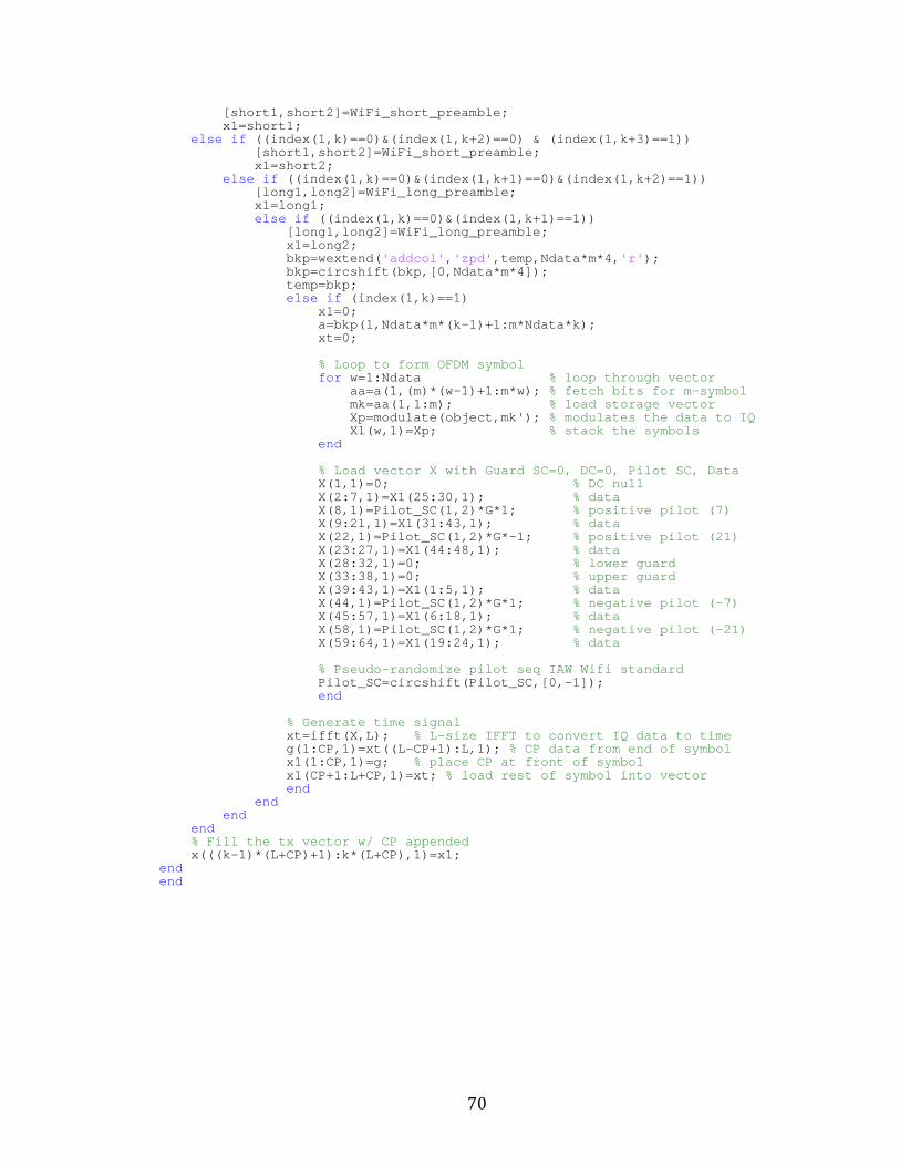
70
[short1,short2]=WiFi_short_preamble; x1=short1; else if ((index(1,k)==0)&(index(1,k+2)==0) & (index(1,k+3) ==1)) [short1,short2]=WiFi_short_preamble; x1=short2; else if ((index(1,k)==0)&(index(1,k+1)==0)&(index(1,k+2)== 1)) [long1,long2]=WiFi_long_preamble; x1=long1; else if ((index(1,k)==0)&(index(1,k+1)==1)) [long1,long2]=WiFi_long_preamble; x1=long2; bkp=wextend( 'addcol' , 'zpd' ,temp,Ndata*m*4, 'r' ); bkp=circshift(bkp,[0,Ndata*m*4]); temp=bkp; else if (index(1,k)==1) x1=0; a=bkp(1,Ndata*m*(k-1)+1:m*Ndata *k); xt=0; % Loop to form OFDM symbol for w=1:Ndata % loop through vector aa=a(1,(m)*(w-1)+1:m*w); % fetch bits for m-symbol mk=aa(1,1:m); % load storage vector Xp=modulate(object,mk'); % modulates the data to IQ X1(w,1)=Xp; % stack the symbols end % Load vector X with Guard SC=0, DC=0, Pilot SC, Da ta X(1,1)=0; % DC null X(2:7,1)=X1(25:30,1); % data X(8,1)=Pilot_SC(1,2)*G*1; % positive pilot (7) X(9:21,1)=X1(31:43,1); % data X(22,1)=Pilot_SC(1,2)*G*-1; % positive pilot (21) X(23:27,1)=X1(44:48,1); % data X(28:32,1)=0; % lower guard X(33:38,1)=0; % upper guard X(39:43,1)=X1(1:5,1); % data X(44,1)=Pilot_SC(1,2)*G*1; % negative pilot (-7) X(45:57,1)=X1(6:18,1); % data X(58,1)=Pilot_SC(1,2)*G*1; % negative pilot (-21) X(59:64,1)=X1(19:24,1); % data % Pseudo-randomize pilot seq IAW Wifi standard Pilot_SC=circshift(Pilot_SC,[0, -1]); end % Generate time signal xt=ifft(X,L); % L-size IFFT to convert IQ data to time g(1:CP,1)=xt((L-CP+1):L,1); % CP data from end of symbol x1(1:CP,1)=g; % place CP at front of symbol x1(CP+1:L+CP,1)=xt; % load rest of symbol into vector end end end end % Fill the tx vector w/ CP appended x(((k-1)*(L+CP)+1):k*(L+CP),1)=x1; end end
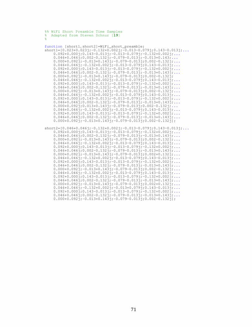
71
%% WiFi Short Preamble Time Samples % Adapted from Steven Schnur [ 19] % function [short1,short2]=WiFi_short_preamble; short1=[0.023+0.023j;-0.132+0.002j;-0.013-0.079j;0. 143-0.013j; ... 0.092+0.000j;0.143-0.013j;-0.013-0.079j;-0.132+ 0.002j; ... 0.046+0.046j;0.002-0.132j;-0.079-0.013j;-0.013+ 0.143; ... 0.000+0.092j;-0.013+0.143j;-0.079-0.013j;0.002- 0.132j; ... 0.046+0.046j;-0.132+0.002j;-0.013-0.079j;0.143- 0.013j; ... 0.092+0.000j;0.143-0.013j;-0.013-0.079j;-0.132+ 0.002j; ... 0.046+0.046j;0.002-0.132j;-0.079-0.013j;-0.013+ 0.143j; ... 0.000+0.092j;-0.013+0.143j;-0.079-0.013j;0.002- 0.132j; 0.046+0.046j;-0.132+0.002j;-0.013-0.079j;0.143- 0.013j; ... 0.092+0.000j;0.143-0.013j;-0.013-0.079j;-0.132+ 0.002j; ... 0.046+0.046j;0.002-0.132j;-0.079-0.013j;-0.013+ 0.143j; ... 0.000+0.092j;-0.013+0.143j;-0.079-0.013j;0.002- 0.132j; ... 0.046+0.046j;-0.132+0.002j;-0.013-0.079j;0.143- 0.013j; ... 0.092+0.000j;0.143-0.013j;-0.013-0.079j;-0.132+ 0.002j; ... 0.046+0.046j;0.002-0.132j;-0.079-0.013j;-0.013+ 0.143j; ... 0.000+0.092j;0.013+0.143j;-0.079-0.013j;0.002-0 .132j; ... 0.046+0.046j;-0.132+0.002j;-0.013-0.079j;0.143- 0.013j; ... 0.092+0.000j;0.143-0.013j;-0.013-0.079j;-0.132+ 0.002j; ... 0.046+0.046j;0.002-0.132j;-0.079-0.013j;-0.013+ 0.143j; ... 0.000+0.092j;-0.013+0.143j;-0.079-0.013j;0.002- 0.132j]; short2=[0.046+0.046j;-0.132+0.002j;-0.013-0.079j;0. 143-0.013j; ... 0.092+0.000j;0.143-0.013j;-0.013-0.079j;-0.132+ 0.002j; ... 0.046+0.046j;0.002-0.132j;-0.079-0.013j;-0.013+ 0.143j; ... 0.000+0.092j;-0.013+0.143j;-0.079-0.013j;0.002- 0.132j; ... 0.046+0.046j;-0.132+0.002j;-0.013-0.079j;0.143- 0.013j; ... 0.092+0.000j;0.143-0.013j;-0.013-0.079j;-0.132+ 0.002j; ... 0.046+0.046j;0.002-0.132j;-0.079-0.013j;-0.013+ 0.143j; ... 0.000+0.092j;-0.013+0.143j;-0.079-0.013j;0.002+ 0.132j; ... 0.046+0.046j;-0.132+0.002j;-0.013-0.079j;0.143- 0.013j; ... 0.092+0.000j;0.143-0.013j;-0.013-0.079j;-0.132+ 0.002j; ... 0.046+0.046j;0.002-0.132j;-0.079-0.013j;-0.013+ 0.143j; ... 0.000+0.092j;-0.013+0.143j;-0.079-0.013j;0.002- 0.132j; ... 0.046+0.046j;-0.132+0.002j;-0.013-0.079j;0.143- 0.013j; ... 0.092+0.000j;0.143-0.013j;-0.013-0.079j;-0.132+ 0.002j; ... 0.046+0.046j;0.002-0.132j;-0.079-0.013j;-0.013+ 0.143j; ... 0.000+0.092j;-0.013+0.143j;-0.079-0.013j;0.002+ 0.132j; ... 0.046+0.046j;-0.132+0.002j;-0.013+0.079j;0.143- 0.013j; ... 0.092+0.000j;0.143-0.013j;-0.013-0.079j;-0.132+ 0.002j; ... 0.046+0.046j;0.002-0.132j;-0.079-0.013j;-0.013+ 0.143j; ... 0.000+0.092j;-0.013+0.143j;-0.079-0.013j;0.002- 0.132j];
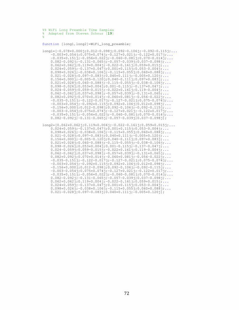
72
%% WiFi Long Preamble Time Samples % Adapted from Steven Schnur [ 19] % function [long1,long2]=WiFi_long_preamble; long1=[-0.078+0.000j;0.012-0.098j;0.092-0.106j;-0.0 92-0.115j; ... -0.003+0.054j;0.075+0.074j;-0.127+0.021j;-0.122 +0.017j; ... -0.035+0.151j;-0.056+0.022j;-0.060-0.081j;0.070 -0.014j; ... 0.082-0.092j;-0.131-0.065j;-0.057-0.039j;0.037- 0.098j; ... 0.062+0.062j;0.119+0.004j;-0.022-0.161j;0.059+0 .015j; ... 0.024+0.059j;-0.137+0.047j;0.001+0.115j;0.053-0 .004j; ... 0.098+0.026j;-0.038+0.106j;-0.115+0.055j;0.060+ 0.088j; ... 0.021-0.028j;0.097-0.083j;0.040+0.111j;-0.005+0 .120j; ... 0.156+0.000j;-0.005-0.120j;0.040-0.111j;0.097+0 .083j; ... 0.021+0.028j;0.060-0.088j;-0.115-0.055j;-0.038- 0.106j; ... 0.098-0.026j;0.053+0.004j;0.001-0.115j;-0.137+0 .047j; ... 0.024-0.059j;0.059-0.015j;-0.022+0.161j;0.119-0 .004j; ... 0.062-0.062j;0.037+0.098j;-0.057+0.039j;-0.131+ 0.065; ... 0.082+0.092j;0.070+0.014j;-0.060+0.081j;-0.056- 0.022j; ... -0.035-0.151j;-0.122-0.017j;-0.127-0.021j;0.075 -0.074j; ... -0.003+0.054j;-0.092+0.115j;0.092+0.106j;0.012+ 0.098j; ... -0.156+0.000j;0.012-0.098j;0.092-0.106j;-0.092- 0.115j; ... -0.003-0.054j;0.075+0.074j;-0.127+0.021j;-0.122 +0.017j; ... -0.035+0.151j;-0.056+0.022j;-0.060-0.081j;0.070 -0.014j; ... 0.082-0.092j;-0.131-0.065j;-0.057-0.039j;0.037- 0.098j]; long2=[0.062+0.062j;0.119+0.004j;-0.022-0.161j;0.05 9+0.015j; ... 0.024+0.059j;-0.137+0.047j;0.001+0.115j;0.053-0 .004j; ... 0.098+0.026j;-0.038+0.106j;-0.115+0.055j;0.060+ 0.088j; ... 0.021-0.028j;0.097-0.083j;0.040+0.111j;-0.005+0 .120j; ... 0.156+0.000j;-0.005-0.120j;0.040-0.111j;0.097+0 .083j; ... 0.021+0.028j;0.060-0.088j;-0.115-0.055j;-0.038- 0.106j; ... 0.098-0.026j;0.053+0.004j;0.001-0.115j;-0.137-0 .047j; ... 0.024-0.059j;0.059-0.015j;-0.022+0.161j;0.119-0 .004j; ... 0.062-0.062j;0.037+0.098j;-0.057+0.039j;-0.131+ 0.065j; ... 0.082+0.092j;0.070+0.014j;-0.060+0.081j;-0.056- 0.022j; ... -0.035-0.151j;-0.122-0.017j;-0.127-0.021j;0.075 -0.074j; ... -0.003+0.054j;-0.092+0.115j;0.092+0.106j;0.012+ 0.098j; ... -0.156+0.000j;0.012-0.098j;0.092-0.106j;-0.092- 0.115j; ... -0.003-0.054j;0.075+0.074j;-0.127+0.021j;-0.122 +0.017j; ... -0.035+0.151j;-0.056+0.022j;-0.060-0.081j;0.070 -0.014j; ... 0.082-0.092j;-0.131-0.065j;-0.057-0.039j;0.037- 0.098j; ... 0.062+0.062j;0.119+0.004j;-0.022-0.161j;0.059+0 .015j; ... 0.024+0.059j;-0.137+0.047j;0.001+0.115j;0.053-0 .004j; ... 0.098+0.026j;-0.038+0.106j;-0.115+0.055j;0.060+ 0.088j; ... 0.021-0.028j;0.097-0.083j;0.040+0.111j;-0.005+0 .120j];
73
%% Spatial Sign Cyclic Correlation Estimator w/ Pha se Compensation % function [lambda,R] = sscce_pc(x,alpha,phi,lag) N=length(x); % SSF function via CORDIC [theta,r]=cart2pol(real(x),imag(x)); [xr,xi]=pol2cart(theta,1); Sx=xr+j*xi; Sx=Sx'; Sxl=[zeros(1,N-1), Sx, zeros(1,N-1)]; if nargin==2 % Full Autocorrelation R=zeros(1,2*N-1); for lags=1:2*N-1 for n=1:N R(lags)=R(lags)+conj(Sx(n))*Sxl(n+lags- 1)*exp(-j*2*pi*alpha*n); end end else if nargin==4 % Discrete autocorrelation M=length(lag); R=zeros(1,M); for lags=1:M for n=1:N R(lags)=R(lags)+conj(Sx(n))*Sxl(n+(N-la g(lags))-1)*exp(-j*(2*pi*alpha*n+phi(lags))); end end end end R=R./N; lambda=N/2*abs(sum(R))^2;

74
APPENDIX B
HDL CODE
-- Author: Sean Hamlin -- Date: February 13, 2016 -- --------------------------------------------------- ----------------- -- Module Overview --------------------------------------------------- ----------------- -- This module computes the Dual-Lag, Spatial Sign Cyclic -- Correlation Estimate with Cyclic Phase Compensat ion for a -- baseband input signal x_real and x_imag over N i nput samples. -- The test statistic value is calculated and compa red against the -- threshold value. The value of the threshold is calculated -- according to the desired probability of false al arm (Pfa) as: -- -- threshold = gaminv(1-Pfa,1,1)*2^(DATA_W-1)/(2^ (N-4)) -- -- If the computed test statistic exceeds the thres hold value input, -- the signal detect output is asserted. The test statistic value -- is provided as an output that is valid at the in sertion of the -- valid_out signal. The baseband input samples ar e clocked into the -- module according to the assertion of valid_in. However, the -- estimation routine calculates at the clk rate, a llowing more -- rapid detection. Also, the detection estimate u ses a moving -- average for the correlation of the test statisti c, allowing -- constant comparison against the threshold. This module is -- parameterized with the following instantiation g enerics: -- --------------------------------------------------- ----------------- -- Module Instantiation Generics --------------------------------------------------- ----------------- -- DATA_W : The width of the baseband input and -- output signals. -- -- LEAD_LAG : The autocorrelation sample lead and lag -- values. -- -- ALPHA : The cyclic frequency value in Hz/Fs. -- -- PHI : The cyclic compensation value. -- -- MAX_SAMPLES : The number of input samples to us e in the -- moving average calculation. Device -- memory resources scale according to this -- value. -- -- ROUNDING_ENABLE : Enables rounding in the multip lication -- output stages. -- -- N_W : This is a calculated generic. Do not mo dify. --------------------------------------------------- ----------------- library ieee; use ieee.std_logic_1164.all; use ieee.numeric_std.all; use ieee.math_real.all; library ieee_proposed; use ieee_proposed.fixed_float_types.all; use ieee_proposed.fixed_pkg.all; entity sscce is GENERIC( DATA_W : integer := 18; LEAD_LAG : integer := 64; ALPHA : real := -1.0/80.0; PHI : real := -64.0/80.0; MAX_SAMPLES : integer := 4096; ROUNDING_ENABLE: boolean := false; N_W : integer := integer(ceil(log2(real(MAX_SAMP LES))))); PORT( reset_n : in std_logic;
75
clk : in std_logic; N : in std_logic_vector(N_W downto 0); threshold : in std_logic_vector(DATA_W-1 downto 0); valid_in : in std_logic; x_real : in std_logic_vector(DATA_W-1 downto 0) ; x_imag : in std_logic_vector(DATA_W-1 downto 0) ; valid_out : out std_logic; statistic : out std_logic_vector(DATA_W-1 downto 0); signal_detect : out std_logic); end sscce; architecture rtl of sscce is -- Function to generate the phase increment value f rom the desired -- normalized frequency and the phase accumulator w idth function freq_to_int(freq : in real; phase_accum_w : in integer) return integer is begin return integer(round(freq*real(2**phase_accum_w))); end freq_to_int; -- Function to generate the phase offset value from the desired -- normalized phase and the phase accumulator width function phase_to_int(phase : in real; phase_accum_ w : in integer) return integer is begin return integer(round(phase*real(2**phase_accum_w))) ; end phase_to_int; component ssf generic( DATA_W : integer := 18; CORDIC_ITERATIONS : integer := 18); port( reset_n : in std_logic; clk : in std_logic; valid_in : in std_logic; x : in std_logic_vector(DATA_W-1 downto 0); y : in std_logic_vector(DATA_W-1 downto 0); valid_out : out std_logic; Sx : out std_logic_vector(DATA_W-1 downto 0); Sy : out std_logic_vector(DATA_W-1 downto 0)); end component; component lead_lag_shift_reg generic( DATA_W : integer := 18; LEAD_LAG : integer := 64); port( reset_n : in std_logic; clk : in std_logic; valid_in : in std_logic; x_in : in std_logic_vector(DATA_W-1 downto 0); valid_out : out std_logic; x_out : out std_logic_vector(DATA_W-1 downto 0); x_lead : out std_logic_vector(DATA_W-1 downto 0) ; x_lag : out std_logic_vector(DATA_W-1 downto 0)) ; end component; component fixed_nco generic( DATA_W : integer := 18; PHASE_ACCUM_W : integer := 32; PHASE_INC : integer := 1000; PHASE_OFFSET : integer := 0; ITERATIONS : integer := 18); port( reset_n : in std_logic; clk : in std_logic; ce : in std_logic; valid_out : out std_logic; x : out std_logic_vector(DATA_W-1 downto 0); y : out std_logic_vector(DATA_W-1 downto 0)); end component; component complex_mult generic( DATA_W : integer := 18; SCALING_BY_2 : integer := 0; ROUNDING_ENABLE : boolean := false); port( reset_n : in std_logic;
76
clk : in std_logic; valid_in : in std_logic; a_real : in std_logic_vector(DATA_W-1 downto 0); a_imag : in std_logic_vector(DATA_W-1 downto 0); b_real : in std_logic_vector(DATA_W-1 downto 0); b_imag : in std_logic_vector(DATA_W-1 downto 0); valid_out : out std_logic; c_real : out std_logic_vector(DATA_W-1 downto 0) ; c_imag : out std_logic_vector(DATA_W-1 downto 0) ); end component; component moving_average generic( DATA_W : integer := 18; MAX_POINTS : integer := 2048; SCALING_BY_2 : integer := 0); port( reset_n : in std_logic; clk : in std_logic; N : in std_logic_vector(N_W downto 0); valid_in : in std_logic; x : in std_logic_vector(DATA_W-1 downto 0); valid_out : out std_logic; y : out std_logic_vector(DATA_W-1 downto 0)); end component; component real_mult generic( DATA_W : integer := 18; ROUNDING_ENABLE : boolean := false); port( reset_n : in std_logic; clk : in std_logic; valid_in : in std_logic; a : in std_logic_vector(DATA_W-1 downto 0); b : in std_logic_vector(DATA_W-1 downto 0); valid_out : out std_logic; c : out std_logic_vector(DATA_W-1 downto 0)); end component; -- SSF signals signal Sx : std_logic_vector(DATA_W-1 downto 0); signal Sy : std_logic_vector(DATA_W-1 downto 0); signal valid_norm : std_logic; -- Lead/Lag signals subtype x_range is natural range 2*DATA_W-1 downto DATA_W; subtype y_range is natural range DATA_W-1 downto 0; signal xy_nom : std_logic_vector(2*DATA_W-1 downto 0); signal xy_lead : std_logic_vector(2*DATA_W-1 downt o 0); signal xy_lag : std_logic_vector(2*DATA_W-1 downto 0); signal x_nom : std_logic_vector(DATA_W-1 downto 0) ; signal y_nom : std_logic_vector(DATA_W-1 downto 0) ; signal x_lead : std_logic_vector(DATA_W-1 downto 0 ); signal y_lead : std_logic_vector(DATA_W-1 downto 0 ); signal x_lag : std_logic_vector(DATA_W-1 downto 0) ; signal y_lag : std_logic_vector(DATA_W-1 downto 0) ; signal valid_lead_lag : std_logic; -- Correlation product signals signal x_lead_prod : std_logic_vector(DATA_W-1 down to 0); signal y_lead_prod : std_logic_vector(DATA_W-1 down to 0); signal x_lag_prod : std_logic_vector(DATA_W-1 downt o 0); signal y_lag_prod : std_logic_vector(DATA_W-1 downt o 0); signal valid_lead_prod : std_logic; signal valid_lag_prod : std_logic; -- NCO signals signal alpha_phi_x : std_logic_vector(DATA_W-1 down to 0); signal alpha_phi_y : std_logic_vector(DATA_W-1 down to 0); signal alpha_x : std_logic_vector(DATA_W-1 downto 0); signal alpha_y : std_logic_vector(DATA_W-1 downto 0); signal valid_nco : std_logic; -- Cyclic correlation product and sum signals signal x_lead_cyc_prod : signed(DATA_W-1 downto 0); signal y_lead_cyc_prod : signed(DATA_W-1 downto 0); signal x_lag_cyc_prod : signed(DATA_W-1 downto 0); signal y_lag_cyc_prod : signed(DATA_W-1 downto 0); signal valid_lead_cyc : std_logic; signal valid_lag_cyc : std_logic;
77
signal x_corr_sum : signed(DATA_W-1 downto 0); signal y_corr_sum : signed(DATA_W-1 downto 0); signal valid_corr_sum : std_logic; -- Moving average signals signal x_corr : std_logic_vector(DATA_W-1 downto 0 ); signal y_corr : std_logic_vector(DATA_W-1 downto 0 ); signal valid_x_corr : std_logic; signal valid_y_corr : std_logic; -- Squaring operation signals signal x_corr_squared : unsigned(DATA_W-1 downto 0) ; signal y_corr_squared : unsigned(DATA_W-1 downto 0) ; signal xy_sum : unsigned(DATA_W-1 downto 0); signal valid_xc : std_logic; signal valid_yc : std_logic; begin norm : ssf generic map( DATA_W => DATA_W, CORDIC_ITERATIONS => DATA_W) port map( reset_n => reset_n, clk => clk, valid_in => valid_in, x => x_real, y => x_imag, valid_out => valid_norm, Sx => Sx, Sy => Sy); lags : lead_lag_shift_reg generic map( DATA_W => 2*DATA_W, LEAD_LAG => LEAD_LAG) port map( reset_n => reset_n, clk => clk, valid_in => valid_norm, x_in => Sx & Sy, valid_out => valid_lead_lag, x_out => xy_nom, x_lead => xy_lead, x_lag => xy_lag); x_nom <= xy_nom(x_range); y_nom <= xy_nom(y_range); x_lead <= xy_lead(x_range); y_lead <= xy_lead(y_range); x_lag <= xy_lag(x_range); y_lag <= xy_lag(y_range); lead_prod : complex_mult generic map( DATA_W => DATA_W, ROUNDING_ENABLE => ROUNDING_ENABLE) port map( reset_n => reset_n, clk => clk, valid_in => valid_lead_lag, a_real => x_lead, a_imag => y_lead, b_real => x_nom, b_imag => std_logic_vector(-signed(y_nom)), valid_out => valid_lead_prod, c_real => x_lead_prod, c_imag => y_lead_prod); lag_prod : complex_mult generic map( DATA_W => DATA_W, ROUNDING_ENABLE => ROUNDING_ENABLE) port map( reset_n => reset_n, clk => clk, valid_in => valid_lead_lag, a_real => x_lag, a_imag => y_lag, b_real => x_nom,
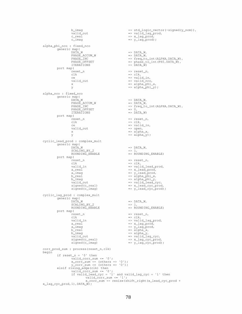
78
b_imag => std_logic_vector(-signed(y_nom)), valid_out => valid_lag_prod, c_real => x_lag_prod, c_imag => y_lag_prod); alpha_phi_nco : fixed_nco generic map( DATA_W => DATA_W, PHASE_ACCUM_W => DATA_W, PHASE_INC => freq_to_int(ALPHA,DATA_W), PHASE_OFFSET => phase_to_int(PHI,DATA_W), ITERATIONS => DATA_W) port map( reset_n => reset_n, clk => clk, ce => valid_in, valid_out => valid_nco, x => alpha_phi_x, y => alpha_phi_y); alpha_nco : fixed_nco generic map( DATA_W => DATA_W, PHASE_ACCUM_W => DATA_W, PHASE_INC => freq_to_int(ALPHA,DATA_W), PHASE_OFFSET => 0, ITERATIONS => DATA_W) port map( reset_n => reset_n, clk => clk, ce => valid_in, valid_out => open, x => alpha_x, y => alpha_y); cyclic_lead_prod : complex_mult generic map( DATA_W => DATA_W, SCALING_BY_2 => 1, ROUNDING_ENABLE => ROUNDING_ENABLE) port map( reset_n => reset_n, clk => clk, valid_in => valid_lead_prod, a_real => x_lead_prod, a_imag => y_lead_prod, b_real => alpha_phi_x, b_imag => alpha_phi_y, valid_out => valid_lead_cyc, signed(c_real) => x_lead_cyc_prod, signed(c_imag) => y_lead_cyc_prod); cyclic_lag_prod : complex_mult generic map( DATA_W => DATA_W, SCALING_BY_2 => 1, ROUNDING_ENABLE => ROUNDING_ENABLE) port map( reset_n => reset_n, clk => clk, valid_in => valid_lag_prod, a_real => x_lag_prod, a_imag => y_lag_prod, b_real => alpha_x, b_imag => alpha_y, valid_out => valid_lag_cyc, signed(c_real) => x_lag_cyc_prod, signed(c_imag) => y_lag_cyc_prod); corr_prod_sum : process(reset_n,clk) begin if reset_n = '0' then valid_corr_sum <= '0'; x_corr_sum <= (others => '0'); y_corr_sum <= (others => '0'); elsif rising_edge(clk) then valid_corr_sum <= '0'; if valid_lead_cyc = '1' and valid_lag_cyc = '1' t hen valid_corr_sum <= '1'; x_corr_sum <= resize(shift_right(x_lead_cyc_prod + x_lag_cyc_prod,1),DATA_W);
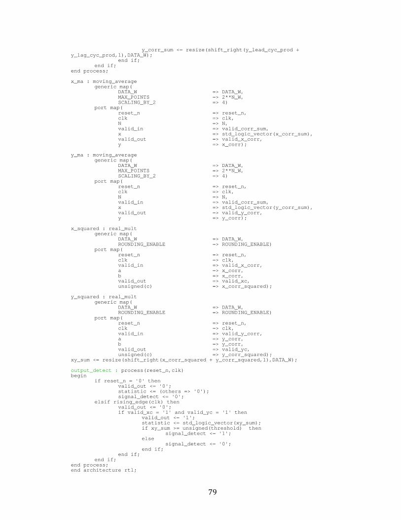
79
y_corr_sum <= resize(shift_right(y_lead_cyc_prod + y_lag_cyc_prod,1),DATA_W); end if; end if; end process; x_ma : moving_average generic map( DATA_W => DATA_W, MAX_POINTS => 2**N_W, SCALING_BY_2 => 4) port map( reset_n => reset_n, clk => clk, N => N, valid_in => valid_corr_sum, x => std_logic_vector(x_corr_sum), valid_out => valid_x_corr, y => x_corr); y_ma : moving_average generic map( DATA_W => DATA_W, MAX_POINTS => 2**N_W, SCALING_BY_2 => 4) port map( reset_n => reset_n, clk => clk, N => N, valid_in => valid_corr_sum, x => std_logic_vector(y_corr_sum), valid_out => valid_y_corr, y => y_corr); x_squared : real_mult generic map( DATA_W => DATA_W, ROUNDING_ENABLE => ROUNDING_ENABLE) port map( reset_n => reset_n, clk => clk, valid_in => valid_x_corr, a => x_corr, b => x_corr, valid_out => valid_xc, unsigned(c) => x_corr_squared); y_squared : real_mult generic map( DATA_W => DATA_W, ROUNDING_ENABLE => ROUNDING_ENABLE) port map( reset_n => reset_n, clk => clk, valid_in => valid_y_corr, a => y_corr, b => y_corr, valid_out => valid_yc, unsigned(c) => y_corr_squared); xy_sum <= resize(shift_right(x_corr_squared + y_cor r_squared,1),DATA_W); output_detect : process(reset_n,clk) begin if reset_n = '0' then valid_out <= '0'; statistic <= (others => '0'); signal_detect <= '0'; elsif rising_edge(clk) then valid_out <= '0'; if valid_xc = '1' and valid_yc = '1' then valid_out <= '1'; statistic <= std_logic_vector(xy_sum); if xy_sum >= unsigned(threshold) then signal_detect <= '1'; else signal_detect <= '0'; end if; end if; end if; end process; end architecture rtl;
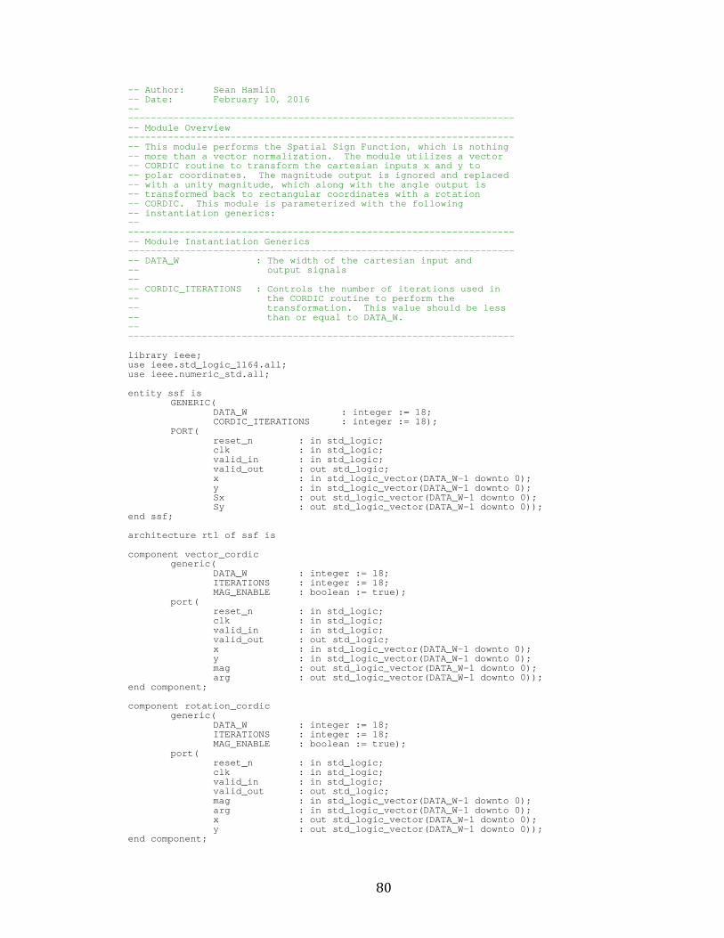
80
-- Author: Sean Hamlin -- Date: February 10, 2016 -- --------------------------------------------------- ----------------- -- Module Overview --------------------------------------------------- ----------------- -- This module performs the Spatial Sign Function, which is nothing -- more than a vector normalization. The module ut ilizes a vector -- CORDIC routine to transform the cartesian inputs x and y to -- polar coordinates. The magnitude output is igno red and replaced -- with a unity magnitude, which along with the ang le output is -- transformed back to rectangular coordinates with a rotation -- CORDIC. This module is parameterized with the f ollowing -- instantiation generics: -- --------------------------------------------------- ----------------- -- Module Instantiation Generics --------------------------------------------------- ----------------- -- DATA_W : The width of the cartesian input and -- output signals -- -- CORDIC_ITERATIONS : Controls the number of itera tions used in -- the CORDIC routine to perform the -- transformation. This value should be less -- than or equal to DATA_W. -- --------------------------------------------------- ----------------- library ieee; use ieee.std_logic_1164.all; use ieee.numeric_std.all; entity ssf is GENERIC( DATA_W : integer := 18; CORDIC_ITERATIONS : integer := 18); PORT( reset_n : in std_logic; clk : in std_logic; valid_in : in std_logic; valid_out : out std_logic; x : in std_logic_vector(DATA_W-1 downto 0); y : in std_logic_vector(DATA_W-1 downto 0); Sx : out std_logic_vector(DATA_W-1 downto 0); Sy : out std_logic_vector(DATA_W-1 downto 0)); end ssf; architecture rtl of ssf is component vector_cordic generic( DATA_W : integer := 18; ITERATIONS : integer := 18; MAG_ENABLE : boolean := true); port( reset_n : in std_logic; clk : in std_logic; valid_in : in std_logic; valid_out : out std_logic; x : in std_logic_vector(DATA_W-1 downto 0); y : in std_logic_vector(DATA_W-1 downto 0); mag : out std_logic_vector(DATA_W-1 downto 0); arg : out std_logic_vector(DATA_W-1 downto 0)); end component; component rotation_cordic generic( DATA_W : integer := 18; ITERATIONS : integer := 18; MAG_ENABLE : boolean := true); port( reset_n : in std_logic; clk : in std_logic; valid_in : in std_logic; valid_out : out std_logic; mag : in std_logic_vector(DATA_W-1 downto 0); arg : in std_logic_vector(DATA_W-1 downto 0); x : out std_logic_vector(DATA_W-1 downto 0); y : out std_logic_vector(DATA_W-1 downto 0)); end component;
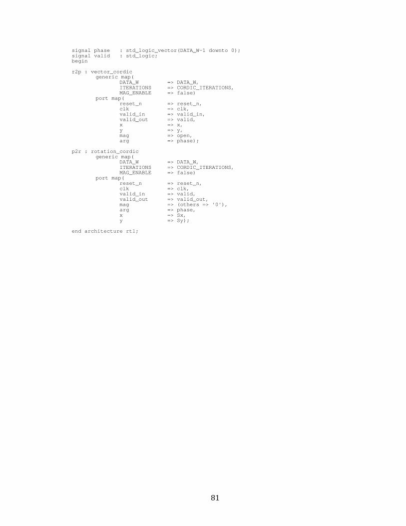
81
signal phase : std_logic_vector(DATA_W-1 downto 0); signal valid : std_logic; begin r2p : vector_cordic generic map( DATA_W => DATA_W, ITERATIONS => CORDIC_ITERATIONS, MAG_ENABLE => false) port map( reset_n => reset_n, clk => clk, valid_in => valid_in, valid_out => valid, x => x, y => y, mag => open, arg => phase); p2r : rotation_cordic generic map( DATA_W => DATA_W, ITERATIONS => CORDIC_ITERATIONS, MAG_ENABLE => false) port map( reset_n => reset_n, clk => clk, valid_in => valid, valid_out => valid_out, mag => (others => '0'), arg => phase, x => Sx, y => Sy); end architecture rtl;
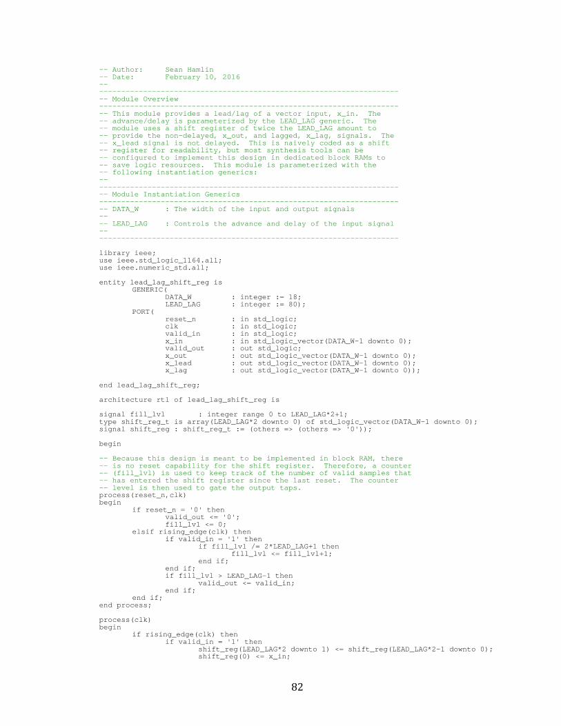
82
-- Author: Sean Hamlin -- Date: February 10, 2016 -- --------------------------------------------------- ----------------- -- Module Overview --------------------------------------------------- ----------------- -- This module provides a lead/lag of a vector inpu t, x_in. The -- advance/delay is parameterized by the LEAD_LAG g eneric. The -- module uses a shift register of twice the LEAD_L AG amount to -- provide the non-delayed, x_out, and lagged, x_la g, signals. The -- x_lead signal is not delayed. This is naively c oded as a shift -- register for readability, but most synthesis too ls can be -- configured to implement this design in dedicated block RAMs to -- save logic resources. This module is parameteri zed with the -- following instantiation generics: -- --------------------------------------------------- ----------------- -- Module Instantiation Generics --------------------------------------------------- ----------------- -- DATA_W : The width of the input and output sign als -- -- LEAD_LAG : Controls the advance and delay of the input signal -- --------------------------------------------------- ----------------- library ieee; use ieee.std_logic_1164.all; use ieee.numeric_std.all; entity lead_lag_shift_reg is GENERIC( DATA_W : integer := 18; LEAD_LAG : integer := 80); PORT( reset_n : in std_logic; clk : in std_logic; valid_in : in std_logic; x_in : in std_logic_vector(DATA_W-1 downto 0); valid_out : out std_logic; x_out : out std_logic_vector(DATA_W-1 downto 0); x_lead : out std_logic_vector(DATA_W-1 downto 0) ; x_lag : out std_logic_vector(DATA_W-1 downto 0)) ; end lead_lag_shift_reg; architecture rtl of lead_lag_shift_reg is signal fill_lvl : integer range 0 to LEAD_LAG*2+1; type shift_reg_t is array(LEAD_LAG*2 downto 0) of s td_logic_vector(DATA_W-1 downto 0); signal shift_reg : shift_reg_t := (others => (other s => '0')); begin -- Because this design is meant to be implemented i n block RAM, there -- is no reset capability for the shift register. Therefore, a counter -- (fill_lvl) is used to keep track of the number o f valid samples that -- has entered the shift register since the last re set. The counter -- level is then used to gate the output taps. process(reset_n,clk) begin if reset_n = '0' then valid_out <= '0'; fill_lvl <= 0; elsif rising_edge(clk) then if valid_in = '1' then if fill_lvl /= 2*LEAD_LAG+1 then fill_lvl <= fill_lvl+1; end if; end if; if fill_lvl > LEAD_LAG-1 then valid_out <= valid_in; end if; end if; end process; process(clk) begin if rising_edge(clk) then if valid_in = '1' then shift_reg(LEAD_LAG*2 downto 1) <= shift_reg(LEAD _LAG*2-1 downto 0); shift_reg(0) <= x_in;

83
end if; end if; end process; x_lead <= shift_reg(0); x_out <= shift_reg(LEAD_LAG) when fill_lvl > LEAD_L AG else (others => '0'); x_lag <= shift_reg(LEAD_LAG*2) when fill_lvl > LEAD _LAG*2 else (others => '0'); end architecture rtl;
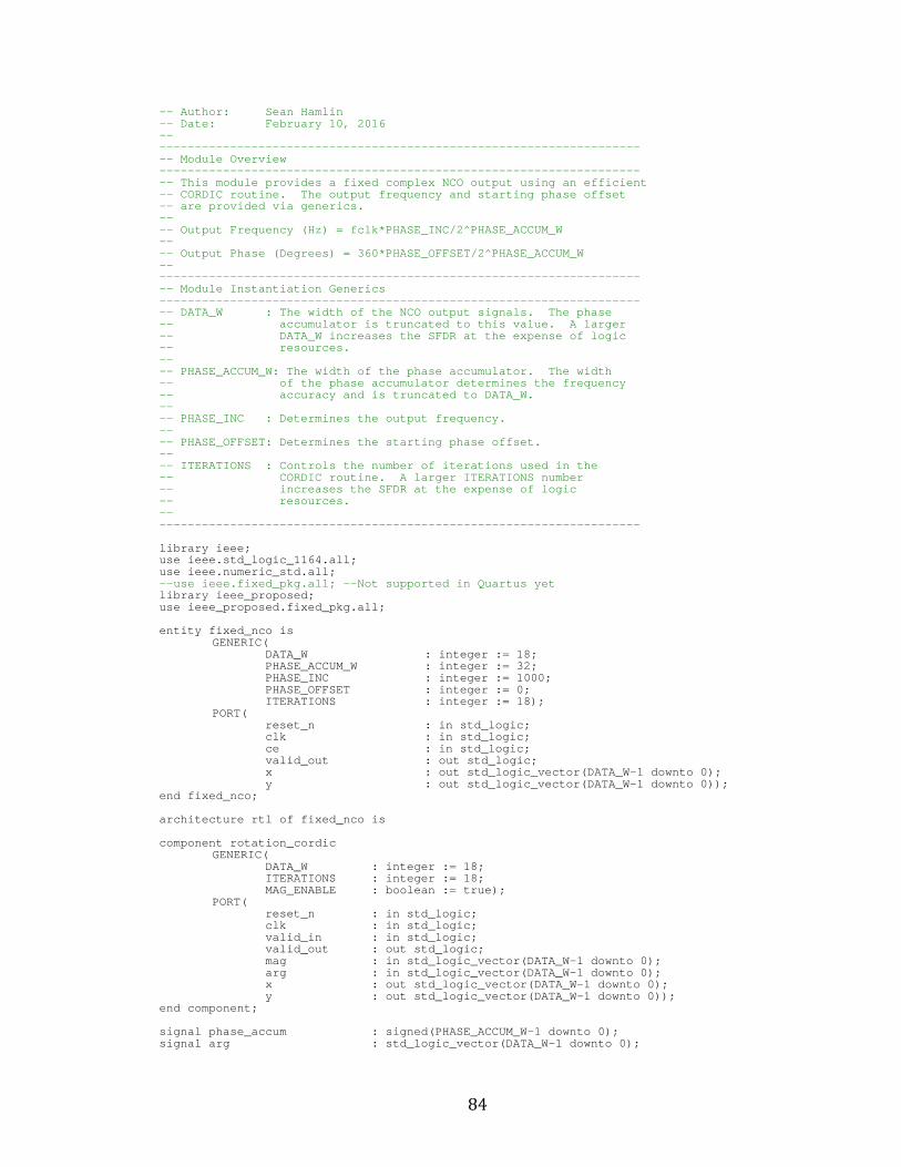
84
-- Author: Sean Hamlin -- Date: February 10, 2016 -- --------------------------------------------------- ----------------- -- Module Overview --------------------------------------------------- ----------------- -- This module provides a fixed complex NCO output using an efficient -- CORDIC routine. The output frequency and starti ng phase offset -- are provided via generics. -- -- Output Frequency (Hz) = fclk*PHASE_INC/2^PHASE_A CCUM_W -- -- Output Phase (Degrees) = 360*PHASE_OFFSET/2^PHAS E_ACCUM_W -- --------------------------------------------------- ----------------- -- Module Instantiation Generics --------------------------------------------------- ----------------- -- DATA_W : The width of the NCO output signals. T he phase -- accumulator is truncated to this value. A la rger -- DATA_W increases the SFDR at the expense of l ogic -- resources. -- -- PHASE_ACCUM_W: The width of the phase accumulato r. The width -- of the phase accumulator determines the frequ ency -- accuracy and is truncated to DATA_W. -- -- PHASE_INC : Determines the output frequency. -- -- PHASE_OFFSET: Determines the starting phase offs et. -- -- ITERATIONS : Controls the number of iterations u sed in the -- CORDIC routine. A larger ITERATIONS number -- increases the SFDR at the expense of logic -- resources. -- --------------------------------------------------- ----------------- library ieee; use ieee.std_logic_1164.all; use ieee.numeric_std.all; --use ieee.fixed_pkg.all; --Not supported in Quartu s yet library ieee_proposed; use ieee_proposed.fixed_pkg.all; entity fixed_nco is GENERIC( DATA_W : integer := 18; PHASE_ACCUM_W : integer := 32; PHASE_INC : integer := 1000; PHASE_OFFSET : integer := 0; ITERATIONS : integer := 18); PORT( reset_n : in std_logic; clk : in std_logic; ce : in std_logic; valid_out : out std_logic; x : out std_logic_vector(DATA_W-1 downto 0); y : out std_logic_vector(DATA_W-1 downto 0)); end fixed_nco; architecture rtl of fixed_nco is component rotation_cordic GENERIC( DATA_W : integer := 18; ITERATIONS : integer := 18; MAG_ENABLE : boolean := true); PORT( reset_n : in std_logic; clk : in std_logic; valid_in : in std_logic; valid_out : out std_logic; mag : in std_logic_vector(DATA_W-1 downto 0); arg : in std_logic_vector(DATA_W-1 downto 0); x : out std_logic_vector(DATA_W-1 downto 0); y : out std_logic_vector(DATA_W-1 downto 0)); end component; signal phase_accum : signed(PHASE_ACCUM_W-1 downto 0); signal arg : std_logic_vector(DATA_W-1 downto 0);
85
begin assert(PHASE_ACCUM_W>=DATA_W) report "PHASE_ACCUM_W must be greater than DATA_W" severity error; process(reset_n,clk) begin if reset_n = '0' then phase_accum <= to_signed(PHASE_OFFSET,PHASE_ACCUM _W); elsif rising_edge(clk) then if ce = '1' then phase_accum <= phase_accum+PHASE_INC; end if; end if; end process; arg <= std_logic_vector(phase_accum(PHASE_ACCUM_W-1 downto PHASE_ACCUM_W-DATA_W)); cordic : rotation_cordic generic map( DATA_W => DATA_W, ITERATIONS => ITERATIONS, MAG_ENABLE => false) port map( reset_n => reset_n, clk => clk, valid_in => ce, valid_out => valid_out, mag => (others => '0'), arg => arg, x => x, y => y); end architecture rtl;
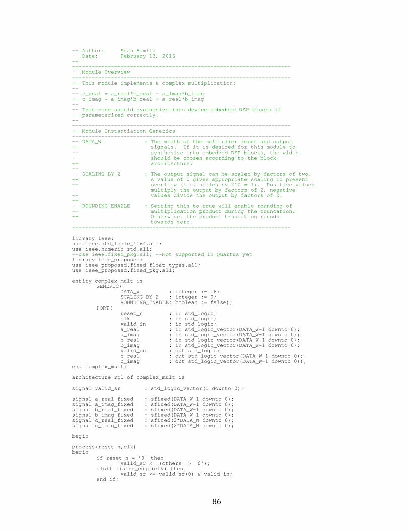
86
-- Author: Sean Hamlin -- Date: February 13, 2016 -- --------------------------------------------------- ----------------- -- Module Overview --------------------------------------------------- ----------------- -- This module implements a complex multiplication: -- -- c_real = a_real*b_real - a_imag*b_imag -- c_imag = a_imag*b_real + a_real*b_imag -- -- This core should synthesize into device embedded DSP blocks if -- parameterized correctly. -- --------------------------------------------------- ----------------- -- Module Instantiation Generics --------------------------------------------------- ----------------- -- DATA_W : The width of the multiplier input and output -- signals. If it is desired for this module t o -- synthesize into embedded DSP blocks, the wid th -- should be chosen according to the block -- architecture. -- -- SCALING_BY_2 : The output signal can be scaled b y factors of two. -- A value of 0 gives appropriate scaling to pr event -- overflow (i.e. scales by 2^0 = 1). Positive values -- multiply the output by factors of 2, negativ e -- values divide the output by factors of 2. -- -- ROUNDING_ENABLE : Setting this to true will enab le rounding of -- multiplication product during the truncation . -- Otherwise, the product truncation rounds -- towards zero. --------------------------------------------------- ----------------- library ieee; use ieee.std_logic_1164.all; use ieee.numeric_std.all; --use ieee.fixed_pkg.all; --Not supported in Quartu s yet library ieee_proposed; use ieee_proposed.fixed_float_types.all; use ieee_proposed.fixed_pkg.all; entity complex_mult is GENERIC( DATA_W : integer := 18; SCALING_BY_2 : integer := 0; ROUNDING_ENABLE: boolean := false); PORT( reset_n : in std_logic; clk : in std_logic; valid_in : in std_logic; a_real : in std_logic_vector(DATA_W-1 downto 0); a_imag : in std_logic_vector(DATA_W-1 downto 0); b_real : in std_logic_vector(DATA_W-1 downto 0); b_imag : in std_logic_vector(DATA_W-1 downto 0); valid_out : out std_logic; c_real : out std_logic_vector(DATA_W-1 downto 0) ; c_imag : out std_logic_vector(DATA_W-1 downto 0) ); end complex_mult; architecture rtl of complex_mult is signal valid_sr : std_logic_vector(1 downto 0); signal a_real_fixed : sfixed(DATA_W-1 downto 0); signal a_imag_fixed : sfixed(DATA_W-1 downto 0); signal b_real_fixed : sfixed(DATA_W-1 downto 0); signal b_imag_fixed : sfixed(DATA_W-1 downto 0); signal c_real_fixed : sfixed(2*DATA_W downto 0); signal c_imag_fixed : sfixed(2*DATA_W downto 0); begin process(reset_n,clk) begin if reset_n = '0' then valid_sr <= (others => '0'); elsif rising_edge(clk) then valid_sr <= valid_sr(0) & valid_in; end if;
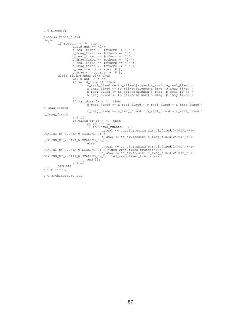
87
end process; process(reset_n,clk) begin if reset_n = '0' then valid_out <= '0'; a_real_fixed <= (others => '0'); a_imag_fixed <= (others => '0'); b_real_fixed <= (others => '0'); b_imag_fixed <= (others => '0'); c_real_fixed <= (others => '0'); c_imag_fixed <= (others => '0'); c_real <= (others => '0'); c_imag <= (others => '0'); elsif rising_edge(clk) then valid_out <= '0'; if valid_in = '1' then a_real_fixed <= to_sfixed(signed(a_real),a_real_ fixed); a_imag_fixed <= to_sfixed(signed(a_imag),a_imag_ fixed); b_real_fixed <= to_sfixed(signed(b_real),b_real_ fixed); b_imag_fixed <= to_sfixed(signed(b_imag),b_imag_ fixed); end if; if valid_sr(0) = '1' then c_real_fixed <= a_real_fixed * b_real_fixed - a_ imag_fixed * b_imag_fixed; c_imag_fixed <= a_imag_fixed * b_real_fixed + a_ real_fixed * b_imag_fixed; end if; if valid_sr(1) = '1' then valid_out <= '1'; if ROUNDING_ENABLE then c_real <= to_slv(resize(c_real_fixed,2*DATA_W-1 -SCALING_BY_2,DATA_W-SCALING_BY_2)); c_imag <= to_slv(resize(c_imag_fixed,2*DATA_W-1 -SCALING_BY_2,DATA_W-SCALING_BY_2)); else c_real <= to_slv(resize(c_real_fixed,2*DATA_W-1 -SCALING_BY_2,DATA_W-SCALING_BY_2,fixed_wrap,fixed_t runcate)); c_imag <= to_slv(resize(c_imag_fixed,2*DATA_W-1 -SCALING_BY_2,DATA_W-SCALING_BY_2,fixed_wrap,fixed_t runcate)); end if; end if; end if; end process; end architecture rtl;
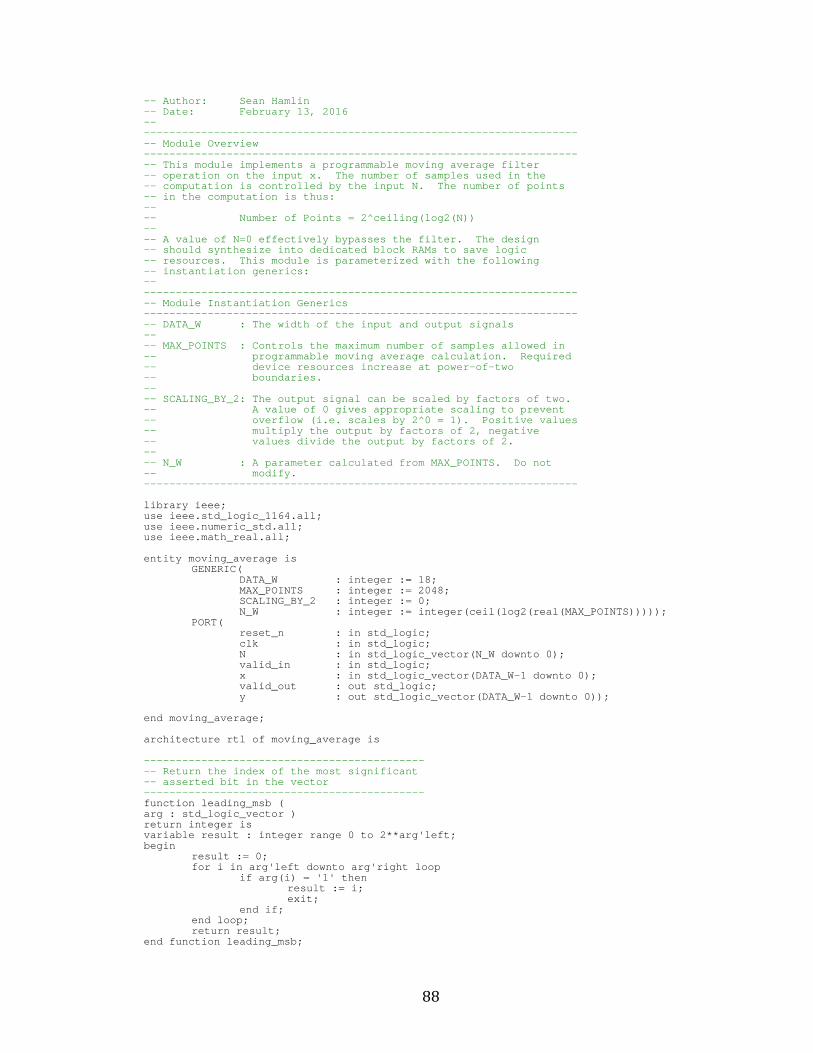
88
-- Author: Sean Hamlin -- Date: February 13, 2016 -- --------------------------------------------------- ----------------- -- Module Overview --------------------------------------------------- ----------------- -- This module implements a programmable moving ave rage filter -- operation on the input x. The number of samples used in the -- computation is controlled by the input N. The n umber of points -- in the computation is thus: -- -- Number of Points = 2^ceiling(log2(N)) -- -- A value of N=0 effectively bypasses the filter. The design -- should synthesize into dedicated block RAMs to s ave logic -- resources. This module is parameterized with th e following -- instantiation generics: -- --------------------------------------------------- ----------------- -- Module Instantiation Generics --------------------------------------------------- ----------------- -- DATA_W : The width of the input and output signa ls -- -- MAX_POINTS : Controls the maximum number of samp les allowed in -- programmable moving average calculation. Req uired -- device resources increase at power-of-two -- boundaries. -- -- SCALING_BY_2: The output signal can be scaled by factors of two. -- A value of 0 gives appropriate scaling to pre vent -- overflow (i.e. scales by 2^0 = 1). Positive values -- multiply the output by factors of 2, negative -- values divide the output by factors of 2. -- -- N_W : A parameter calculated from MAX_POINTS. Do not -- modify. --------------------------------------------------- ----------------- library ieee; use ieee.std_logic_1164.all; use ieee.numeric_std.all; use ieee.math_real.all; entity moving_average is GENERIC( DATA_W : integer := 18; MAX_POINTS : integer := 2048; SCALING_BY_2 : integer := 0; N_W : integer := integer(ceil(log2(real(MAX_POIN TS))))); PORT( reset_n : in std_logic; clk : in std_logic; N : in std_logic_vector(N_W downto 0); valid_in : in std_logic; x : in std_logic_vector(DATA_W-1 downto 0); valid_out : out std_logic; y : out std_logic_vector(DATA_W-1 downto 0)); end moving_average; architecture rtl of moving_average is -------------------------------------------- -- Return the index of the most significant -- asserted bit in the vector -------------------------------------------- function leading_msb ( arg : std_logic_vector ) return integer is variable result : integer range 0 to 2**arg'left; begin result := 0; for i in arg'left downto arg'right loop if arg(i) = '1' then result := i; exit; end if; end loop; return result; end function leading_msb;
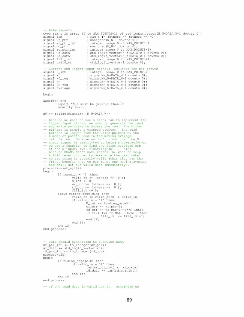
89
-- BRAM signals type ram_t is array (0 to MAX_POINTS-1) of std_logi c_vector(N_W+DATA_W-1 downto 0); signal ram : ram_t := (others => (others => '0')); signal wr_ptr : unsigned(N_W-1 downto 0); signal wr_ptr_int : integer range 0 to MAX_POINTS-1 ; signal rd_ptr : unsigned(N_W-1 downto 0); signal rd_ptr_int : integer range 0 to MAX_POINTS-1 ; signal wr_data : std_logic_vector(N_W+DATA_W-1 dow nto 0); signal rd_data : std_logic_vector(N_W+DATA_W-1 dow nto 0); signal fill_lvl : integer range 0 to MAX_POINTS+1; signal valid_sr : std_logic_vector(1 downto 0); -- Current and lagged input signals, adjusted for b it growth signal N_int : integer range 0 to MAX_POINTS; signal x0 : signed(N_W+DATA_W-1 downto 0); signal x0_reg : signed(N_W+DATA_W-1 downto 0); signal xN : signed(N_W+DATA_W-1 downto 0); signal xN_reg : signed(N_W+DATA_W-1 downto 0); signal average : signed(N_W+DATA_W-1 downto 0); begin assert(N_W>0) report "N_W must be greater than 0" severity error; x0 <= resize(signed(x),N_W+DATA_W); -- Because we want to use a block ram to implement the -- lagged input signal, we need to generate the rea d -- and write pointers to access the ram. The write -- pointer is simply a wrapped counter. The read -- pointer is lagged from the write pointer by the -- number of points used in the moving average -- calculation. Because we don't trust that the N -- input signal is restricted to being a power-of-t wo, -- we use a function to find the first asserted MSB -- of the N input, i.e. floor{log2(N)} . Also, -- because BRAMs don't have resets, we want to keep -- a fill level counter to make sure the read data -- we are using is actually valid (this also has th e -- fringe benefit that we can reset our moving aver age -- and still get out valid data immediately). process(reset_n,clk) begin if reset_n = '0' then valid_sr <= (others => '0'); N_int <= 0; wr_ptr <= (others => '0'); rd_ptr <= (others => '0'); fill_lvl <= 0; elsif rising_edge(clk) then valid_sr <= valid_sr(0) & valid_in; if valid_in = '1' then N_int <= leading_msb(N); wr_ptr <= wr_ptr+1; rd_ptr <= wr_ptr+1-(2**N_int); if fill_lvl /= MAX_POINTS+1 then fill_lvl <= fill_lvl+1; end if; end if; end if; end process; -- This should synthesize to a device BRAM wr_ptr_int <= to_integer(wr_ptr); wr_data <= std_logic_vector(x0); rd_ptr_int <= to_integer(rd_ptr); process(clk) begin if rising_edge(clk) then if valid_in = '1' then ram(wr_ptr_int) <= wr_data; rd_data <= ram(rd_ptr_int); end if; end if; end process; -- If the read data is valid use it. Otherwise we
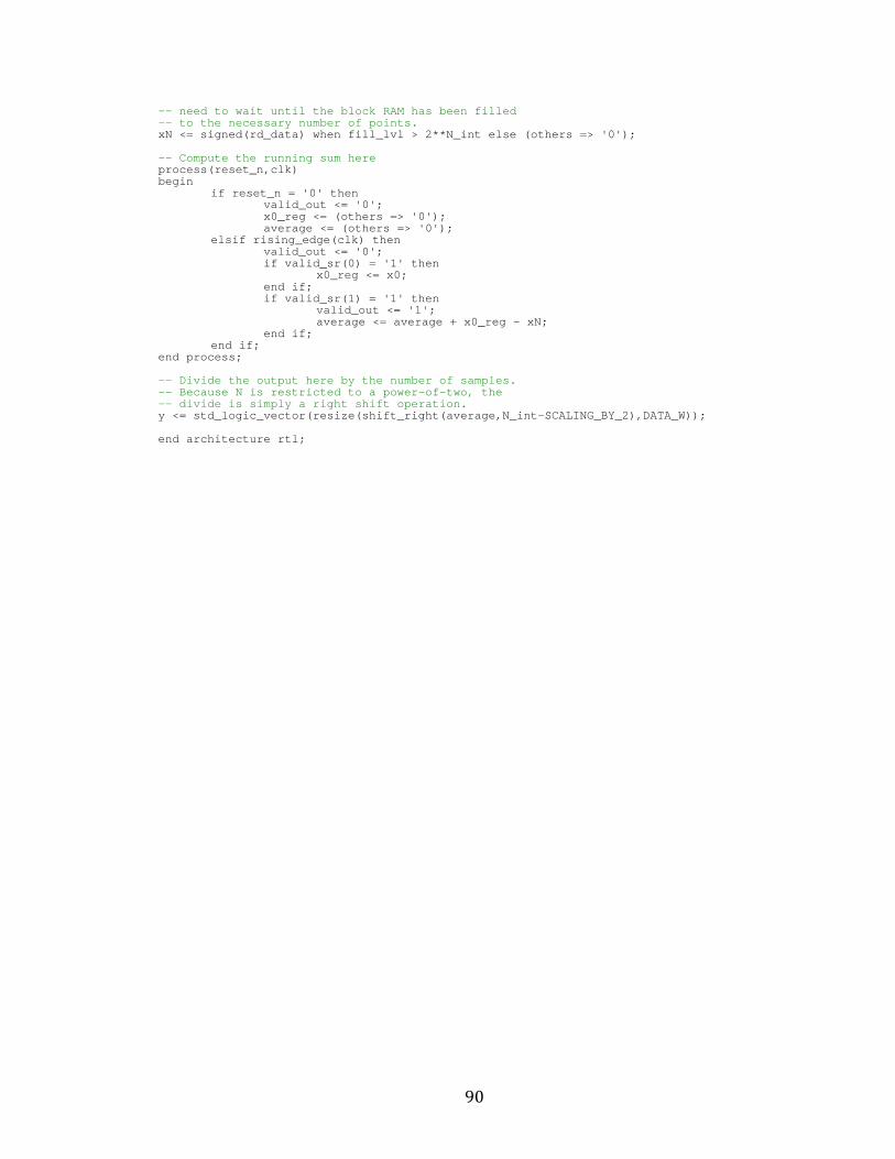
90
-- need to wait until the block RAM has been filled -- to the necessary number of points. xN <= signed(rd_data) when fill_lvl > 2**N_int else (others => '0'); -- Compute the running sum here process(reset_n,clk) begin if reset_n = '0' then valid_out <= '0'; x0_reg <= (others => '0'); average <= (others => '0'); elsif rising_edge(clk) then valid_out <= '0'; if valid_sr(0) = '1' then x0_reg <= x0; end if; if valid_sr(1) = '1' then valid_out <= '1'; average <= average + x0_reg - xN; end if; end if; end process; -- Divide the output here by the number of samples. -- Because N is restricted to a power-of-two, the -- divide is simply a right shift operation. y <= std_logic_vector(resize(shift_right(average,N_ int-SCALING_BY_2),DATA_W)); end architecture rtl;
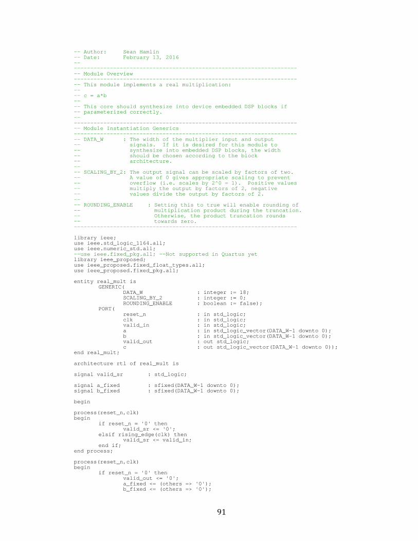
91
-- Author: Sean Hamlin -- Date: February 13, 2016 -- --------------------------------------------------- ----------------- -- Module Overview --------------------------------------------------- ----------------- -- This module implements a real multiplication: -- -- c = a*b -- -- This core should synthesize into device embedded DSP blocks if -- parameterized correctly. -- --------------------------------------------------- ----------------- -- Module Instantiation Generics --------------------------------------------------- ----------------- -- DATA_W : The width of the multiplier input and output -- signals. If it is desired for this module to -- synthesize into embedded DSP blocks, the widt h -- should be chosen according to the block -- architecture. -- -- SCALING_BY_2: The output signal can be scaled by factors of two. -- A value of 0 gives appropriate scaling to pre vent -- overflow (i.e. scales by 2^0 = 1). Positive values -- multiply the output by factors of 2, negative -- values divide the output by factors of 2. -- -- ROUNDING_ENABLE : Setting this to true will enab le rounding of -- multiplication product during the truncation . -- Otherwise, the product truncation rounds -- towards zero. --------------------------------------------------- ----------------- library ieee; use ieee.std_logic_1164.all; use ieee.numeric_std.all; --use ieee.fixed_pkg.all; --Not supported in Quartu s yet library ieee_proposed; use ieee_proposed.fixed_float_types.all; use ieee_proposed.fixed_pkg.all; entity real_mult is GENERIC( DATA_W : integer := 18; SCALING_BY_2 : integer := 0; ROUNDING_ENABLE : boolean := false); PORT( reset_n : in std_logic; clk : in std_logic; valid_in : in std_logic; a : in std_logic_vector(DATA_W-1 downto 0); b : in std_logic_vector(DATA_W-1 downto 0); valid_out : out std_logic; c : out std_logic_vector(DATA_W-1 downto 0)); end real_mult; architecture rtl of real_mult is signal valid_sr : std_logic; signal a_fixed : sfixed(DATA_W-1 downto 0); signal b_fixed : sfixed(DATA_W-1 downto 0); begin process(reset_n,clk) begin if reset_n = '0' then valid_sr <= '0'; elsif rising_edge(clk) then valid_sr <= valid_in; end if; end process; process(reset_n,clk) begin if reset_n = '0' then valid_out <= '0'; a_fixed <= (others => '0'); b_fixed <= (others => '0');
92
c <= (others => '0'); elsif rising_edge(clk) then valid_out <= '0'; if valid_in = '1' then a_fixed <= to_sfixed(signed(a),a_fixed); b_fixed <= to_sfixed(signed(b),b_fixed); end if; if valid_sr = '1' then valid_out <= '1'; if ROUNDING_ENABLE then c <= to_slv(resize(a_fixed * b_fixed,2*DATA_W-2 -SCALING_BY_2,DATA_W-1-SCALING_BY_2)); else c <= to_slv(resize(a_fixed * b_fixed,2*DATA_W-2 -SCALING_BY_2,DATA_W-1-SCALING_BY_2,fixed_wrap,fixed _truncate)); end if; end if; end if; end process; end architecture rtl;
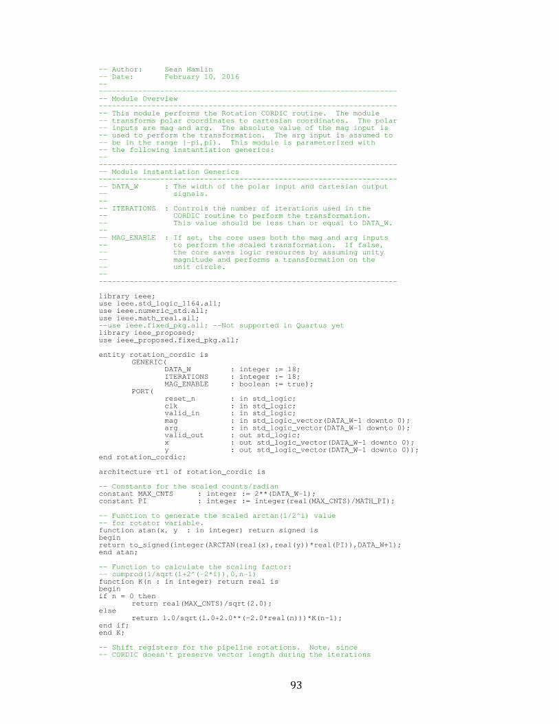
93
-- Author: Sean Hamlin -- Date: February 10, 2016 -- --------------------------------------------------- ----------------- -- Module Overview --------------------------------------------------- ----------------- -- This module performs the Rotation CORDIC routine . The module -- transforms polar coordinates to cartesian coordi nates. The polar -- inputs are mag and arg. The absolute value of t he mag input is -- used to perform the transformation. The arg inp ut is assumed to -- be in the range [-pi,pi). This module is parame terized with -- the following instantiation generics: -- --------------------------------------------------- ----------------- -- Module Instantiation Generics --------------------------------------------------- ----------------- -- DATA_W : The width of the polar input and carte sian output -- signals. -- -- ITERATIONS : Controls the number of iterations u sed in the -- CORDIC routine to perform the transformation. -- This value should be less than or equal to DA TA_W. -- -- MAG_ENABLE : If set, the core uses both the mag and arg inputs -- to perform the scaled transformation. If fal se, -- the core saves logic resources by assuming un ity -- magnitude and performs a transformation on th e -- unit circle. -- --------------------------------------------------- ----------------- library ieee; use ieee.std_logic_1164.all; use ieee.numeric_std.all; use ieee.math_real.all; --use ieee.fixed_pkg.all; --Not supported in Quartu s yet library ieee_proposed; use ieee_proposed.fixed_pkg.all; entity rotation_cordic is GENERIC( DATA_W : integer := 18; ITERATIONS : integer := 18; MAG_ENABLE : boolean := true); PORT( reset_n : in std_logic; clk : in std_logic; valid_in : in std_logic; mag : in std_logic_vector(DATA_W-1 downto 0); arg : in std_logic_vector(DATA_W-1 downto 0); valid_out : out std_logic; x : out std_logic_vector(DATA_W-1 downto 0); y : out std_logic_vector(DATA_W-1 downto 0)); end rotation_cordic; architecture rtl of rotation_cordic is -- Constants for the scaled counts/radian constant MAX_CNTS : integer := 2**(DATA_W-1); constant PI : integer := integer(real(MAX_CNTS)/M ATH_PI); -- Function to generate the scaled arctan(1/2^i) va lue -- for rotator variable. function atan(x, y : in integer) return signed is begin return to_signed(integer(ARCTAN(real(x),real(y))*re al(PI)),DATA_W+1); end atan; -- Function to calculate the scaling factor: -- cumprod(1/sqrt(1+2^(-2*i)),0,n-1) function K(n : in integer) return real is begin if n = 0 then return real(MAX_CNTS)/sqrt(2.0); else return 1.0/sqrt(1.0+2.0**(-2.0*real(n)))*K(n-1); end if; end K; -- Shift registers for the pipeline rotations. Not e, since -- CORDIC doesn't preserve vector length during the iterations
94
-- the x,y shift registers need an additional bit o n top of the -- normal carry bit to accommodate the scaling fact or. type shiftreg_t is array(natural range <>) of signe d; signal x_sr : shiftreg_t(ITERATIONS-1 downto 0)(DA TA_W+1 downto 0); signal y_sr : shiftreg_t(ITERATIONS-1 downto 0)(DA TA_W+1 downto 0); signal angle_sr : shiftreg_t(ITERATIONS-1 downto 0) (DATA_W downto 0); signal valid_sr : std_logic_vector(ITERATIONS+2 dow nto 0); signal mag_int : signed(DATA_W+1 downto 0); signal arg_int : signed(DATA_W downto 0); signal x_fixed : sfixed(DATA_W-1 downto 0); signal y_fixed : sfixed(DATA_W-1 downto 0); begin assert(DATA_W>=ITERATIONS) report "ITERATIONS should not be larger than DATA_ W" severity warning; -- This core can be parameterized to operate in two modes -- according to the MAG_ENABLE generic. If MAG_ENA BLE is -- false, the core ignores the mag input and assume s unity -- gain. This implementation reduces resource util ization -- by setting the initial vector magnitude to the C ORDIC -- scaling factor so as to avoid the rescaling at t he end -- of the routine (and thus saving a multiplier). Otherwise -- the mag input is utilized to create a vector wit h the -- desired vector magnitude. mag_select : if MAG_ENABLE generate signal mag_unsigned : unsigned(DATA_W-1 downto 0); begin mag_unsigned <= unsigned(mag); mag_int <= signed(resize(mag_unsigned,DATA_W+2)) w hen (mag_unsigned <= MAX_CNTS) else to_signed(MAX_CNTS,DATA_W+2); end; else generate mag_int <= to_signed(integer(K(ITERATIONS)),DATA_W +2); end generate mag_select; arg_int <= resize(signed(arg),DATA_W+1); -- CORDIC routine will rotate +/-pi/2 from initial position. -- Therefore, to resolve a 2*pi argument, the initi al (x,y) -- position needs to be chosen based on the argumen t. The -- method used here chooses +/-y based on the sign of the -- argument for simplicity, but other methods are p ossible. process(reset_n,clk) begin if reset_n = '0' then valid_sr <= (others => '0'); x_sr(0) <= (others => '0'); y_sr(0) <= (others => '0'); angle_sr(0) <= (others => '0'); elsif rising_edge(clk) then valid_sr <= valid_sr(ITERATIONS+1 downto 0) & val id_in; if valid_in = '1' then x_sr(0) <= (others => '0'); if arg_int < 0 then y_sr(0) <= -mag_int; angle_sr(0) <= arg_int+MAX_CNTS/2; else y_sr(0) <= mag_int; angle_sr(0) <= arg_int-MAX_CNTS/2; end if; end if; end if; end process; -- Here is the CORDIC routine proper. Basic idea i s to -- examine the sign of the desired angle and if pos itive -- rotate the vector by a positive angle, and negat ive -- conversely. The rotation angles are chosen to b e the -- arctan(1/2^(i-1)) which simplifies the rotations to -- simple power of two shifts. Iteratively subtrac t the -- rotation angle from the desired angle, lather, r inse, -- repeat. pipeline: for i in 1 to ITERATIONS-1 generate begin process(reset_n,clk) begin
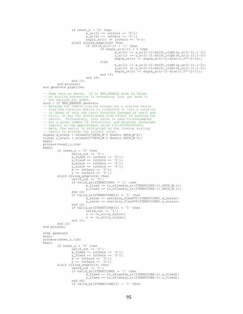
95
if reset_n = '0' then x_sr(i) <= (others => '0'); y_sr(i) <= (others => '0'); angle_sr(i) <= (others => '0'); elsif rising_edge(clk) then if valid_sr(i-1) = '1' then if angle_sr(i-1) < 0 then x_sr(i) <= x_sr(i-1)+shift_right(y_sr(i-1),i-1 ); y_sr(i) <= y_sr(i-1)-shift_right(x_sr(i-1),i-1 ); angle_sr(i) <= angle_sr(i-1)+atan(1,2**(i-1)); else x_sr(i) <= x_sr(i-1)-shift_right(y_sr(i-1),i-1 ); y_sr(i) <= y_sr(i-1)+shift_right(x_sr(i-1),i-1 ); angle_sr(i) <= angle_sr(i-1)-atan(1,2**(i-1)); end if; end if; end if; end process; end generate pipeline; -- Same note as above. If in MAG_ENABLE mode is fa lse, -- no scaling correction is necessary; just get bac k to -- the desired bit width. norm : if MAG_ENABLE generate -- Because the CORDIC routine brings out a scaling factor -- from the rotation matrix to transform it into a rotation -- in terms of only the tan() function instead of c os() and -- sin(), it has the unfortunate side effect of sca ling the -- vector. Fortunately, this value is easy to prec ompute -- for a given number of iterations, and moreover c onverges -- rapidly to the approximate value 1/0.60725293500 9. -- Here, the vector is multiplied by the inverse sc aling -- factor to provide the correct value. signal x_scale : sfixed(2*DATA_W-3 downto DATA_W-2) ; signal y_scale : sfixed(2*DATA_W-3 downto DATA_W-2) ; begin process(reset_n,clk) begin if reset_n = '0' then valid_out <= '0'; x_fixed <= (others => '0'); y_fixed <= (others => '0'); x_scale <= (others => '0'); y_scale <= (others => '0'); x <= (others => '0'); y <= (others => '0'); elsif rising_edge(clk) then valid_out <= '0'; if valid_sr(ITERATIONS) = '1' then x_fixed <= to_sfixed(x_sr(ITERATIONS-1),DATA_W,1 ); y_fixed <= to_sfixed(y_sr(ITERATIONS-1),DATA_W,1 ); end if; if valid_sr(ITERATIONS+1) = '1' then x_scale <= resize(x_fixed*K(ITERATIONS),x_scale) ; y_scale <= resize(y_fixed*K(ITERATIONS),y_scale) ; end if; if valid_sr(ITERATIONS+2) = '1' then valid_out <= '1'; x <= to_slv(x_scale); y <= to_slv(y_scale); end if; end if; end process; else generate begin process(reset_n,clk) begin if reset_n = '0' then valid_out <= '0'; x_fixed <= (others => '0'); y_fixed <= (others => '0'); x <= (others => '0'); y <= (others => '0'); elsif rising_edge(clk) then valid_out <= '0'; if valid_sr(ITERATIONS) = '1' then x_fixed <= to_sfixed(x_sr(ITERATIONS-1),x_fixed) ; y_fixed <= to_sfixed(y_sr(ITERATIONS-1),y_fixed) ; end if; if valid_sr(ITERATIONS+1) = '1' then

96
valid_out <= '1'; x <= to_slv(x_fixed); y <= to_slv(y_fixed); end if; end if; end process; end generate norm; end architecture rtl;
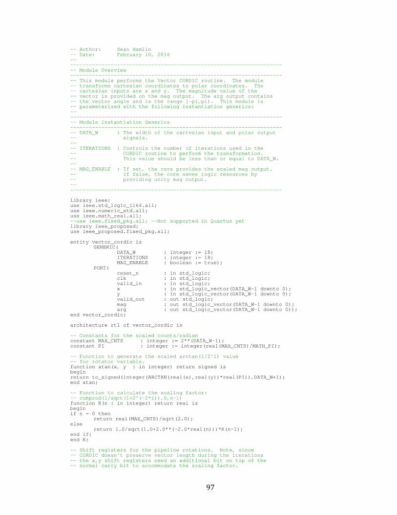
97
-- Author: Sean Hamlin -- Date: February 10, 2016 -- --------------------------------------------------- ----------------- -- Module Overview --------------------------------------------------- ----------------- -- This module performs the Vector CORDIC routine. The module -- transforms cartesian coordinates to polar coordi nates. The -- cartesian inputs are x and y. The magnitude val ue of the -- vector is provided on the mag output. The arg o utput contains -- the vector angle and is the range [-pi,pi). Thi s module is -- parameterized with the following instantiation g enerics: -- --------------------------------------------------- ----------------- -- Module Instantiation Generics --------------------------------------------------- ----------------- -- DATA_W : The width of the cartesian input and p olar output -- signals. -- -- ITERATIONS : Controls the number of iterations u sed in the -- CORDIC routine to perform the transformation. -- This value should be less than or equal to DA TA_W. -- -- MAG_ENABLE : If set, the core provides the scale d mag output. -- If false, the core saves logic resources by -- providing unity mag output. -- --------------------------------------------------- ----------------- library ieee; use ieee.std_logic_1164.all; use ieee.numeric_std.all; use ieee.math_real.all; --use ieee.fixed_pkg.all; --Not supported in Quartu s yet library ieee_proposed; use ieee_proposed.fixed_pkg.all; entity vector_cordic is GENERIC( DATA_W : integer := 18; ITERATIONS : integer := 18; MAG_ENABLE : boolean := true); PORT( reset_n : in std_logic; clk : in std_logic; valid_in : in std_logic; x : in std_logic_vector(DATA_W-1 downto 0); y : in std_logic_vector(DATA_W-1 downto 0); valid_out : out std_logic; mag : out std_logic_vector(DATA_W-1 downto 0); arg : out std_logic_vector(DATA_W-1 downto 0)); end vector_cordic; architecture rtl of vector_cordic is -- Constants for the scaled counts/radian constant MAX_CNTS : integer := 2**(DATA_W-1); constant PI : integer := integer(real(MAX_CNTS)/M ATH_PI); -- Function to generate the scaled arctan(1/2^i) va lue -- for rotator variable. function atan(x, y : in integer) return signed is begin return to_signed(integer(ARCTAN(real(x),real(y))*re al(PI)),DATA_W+1); end atan; -- Function to calculate the scaling factor: -- cumprod(1/sqrt(1+2^(-2*i)),0,n-1) function K(n : in integer) return real is begin if n = 0 then return real(MAX_CNTS)/sqrt(2.0); else return 1.0/sqrt(1.0+2.0**(-2.0*real(n)))*K(n-1); end if; end K; -- Shift registers for the pipeline rotations. Not e, since -- CORDIC doesn't preserve vector length during the iterations -- the x,y shift registers need an additional bit o n top of the -- normal carry bit to accommodate the scaling fact or.
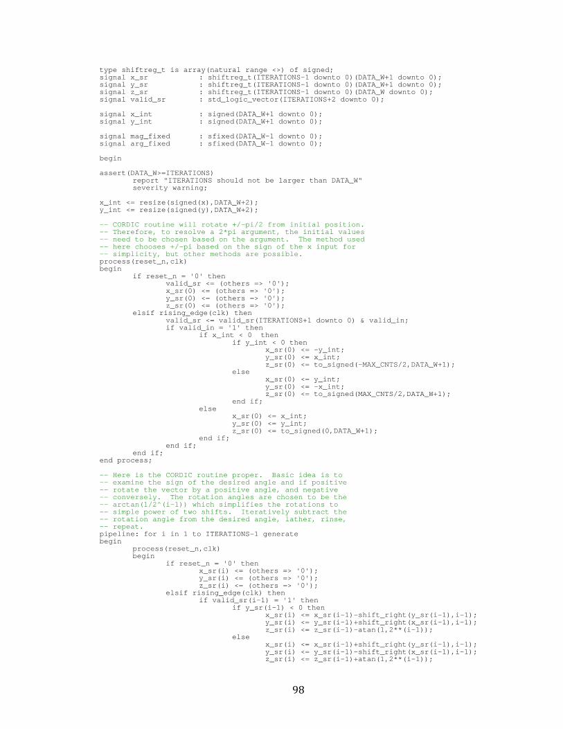
98
type shiftreg_t is array(natural range <>) of signe d; signal x_sr : shiftreg_t(ITERATIONS-1 downto 0)(D ATA_W+1 downto 0); signal y_sr : shiftreg_t(ITERATIONS-1 downto 0)(D ATA_W+1 downto 0); signal z_sr : shiftreg_t(ITERATIONS-1 downto 0)(DA TA_W downto 0); signal valid_sr : std_logic_vector(ITERATIONS+2 dow nto 0); signal x_int : signed(DATA_W+1 downto 0); signal y_int : signed(DATA_W+1 downto 0); signal mag_fixed : sfixed(DATA_W-1 downto 0); signal arg_fixed : sfixed(DATA_W-1 downto 0); begin assert(DATA_W>=ITERATIONS) report "ITERATIONS should not be larger than DATA_ W" severity warning; x_int <= resize(signed(x),DATA_W+2); y_int <= resize(signed(y),DATA_W+2); -- CORDIC routine will rotate +/-pi/2 from initial position. -- Therefore, to resolve a 2*pi argument, the initi al values -- need to be chosen based on the argument. The me thod used -- here chooses +/-pi based on the sign of the x in put for -- simplicity, but other methods are possible. process(reset_n,clk) begin if reset_n = '0' then valid_sr <= (others => '0'); x_sr(0) <= (others => '0'); y_sr(0) <= (others => '0'); z_sr(0) <= (others => '0'); elsif rising_edge(clk) then valid_sr <= valid_sr(ITERATIONS+1 downto 0) & val id_in; if valid_in = '1' then if x_int < 0 then if y_int < 0 then x_sr(0) <= -y_int; y_sr(0) <= x_int; z_sr(0) <= to_signed(-MAX_CNTS/2,DATA_W+1); else x_sr(0) <= y_int; y_sr(0) <= -x_int; z_sr(0) <= to_signed(MAX_CNTS/2,DATA_W+1); end if; else x_sr(0) <= x_int; y_sr(0) <= y_int; z_sr(0) <= to_signed(0,DATA_W+1); end if; end if; end if; end process; -- Here is the CORDIC routine proper. Basic idea i s to -- examine the sign of the desired angle and if pos itive -- rotate the vector by a positive angle, and negat ive -- conversely. The rotation angles are chosen to b e the -- arctan(1/2^(i-1)) which simplifies the rotations to -- simple power of two shifts. Iteratively subtrac t the -- rotation angle from the desired angle, lather, r inse, -- repeat. pipeline: for i in 1 to ITERATIONS-1 generate begin process(reset_n,clk) begin if reset_n = '0' then x_sr(i) <= (others => '0'); y_sr(i) <= (others => '0'); z_sr(i) <= (others => '0'); elsif rising_edge(clk) then if valid_sr(i-1) = '1' then if y_sr(i-1) < 0 then x_sr(i) <= x_sr(i-1)-shift_right(y_sr(i-1),i-1 ); y_sr(i) <= y_sr(i-1)+shift_right(x_sr(i-1),i-1 ); z_sr(i) <= z_sr(i-1)-atan(1,2**(i-1)); else x_sr(i) <= x_sr(i-1)+shift_right(y_sr(i-1),i-1 ); y_sr(i) <= y_sr(i-1)-shift_right(x_sr(i-1),i-1 ); z_sr(i) <= z_sr(i-1)+atan(1,2**(i-1));
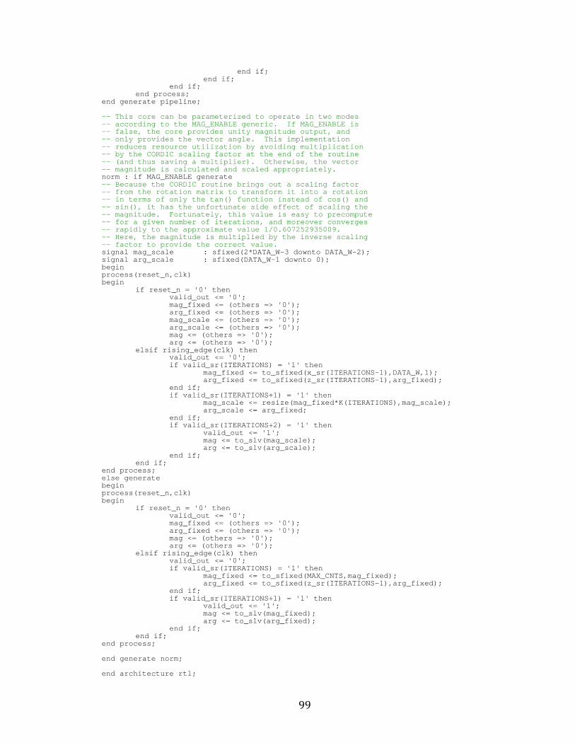
99
end if; end if; end if; end process; end generate pipeline; -- This core can be parameterized to operate in two modes -- according to the MAG_ENABLE generic. If MAG_ENA BLE is -- false, the core provides unity magnitude output, and -- only provides the vector angle. This implementa tion -- reduces resource utilization by avoiding multipl ication -- by the CORDIC scaling factor at the end of the r outine -- (and thus saving a multiplier). Otherwise, the vector -- magnitude is calculated and scaled appropriately . norm : if MAG_ENABLE generate -- Because the CORDIC routine brings out a scaling factor -- from the rotation matrix to transform it into a rotation -- in terms of only the tan() function instead of c os() and -- sin(), it has the unfortunate side effect of sca ling the -- magnitude. Fortunately, this value is easy to p recompute -- for a given number of iterations, and moreover c onverges -- rapidly to the approximate value 1/0.60725293500 9. -- Here, the magnitude is multiplied by the inverse scaling -- factor to provide the correct value. signal mag_scale : sfixed(2*DATA_W-3 downto DATA_W- 2); signal arg_scale : sfixed(DATA_W-1 downto 0); begin process(reset_n,clk) begin if reset_n = '0' then valid_out <= '0'; mag_fixed <= (others => '0'); arg_fixed <= (others => '0'); mag_scale <= (others => '0'); arg_scale <= (others => '0'); mag <= (others => '0'); arg <= (others => '0'); elsif rising_edge(clk) then valid_out <= '0'; if valid_sr(ITERATIONS) = '1' then mag_fixed <= to_sfixed(x_sr(ITERATIONS-1),DATA_W ,1); arg_fixed <= to_sfixed(z_sr(ITERATIONS-1),arg_fi xed); end if; if valid_sr(ITERATIONS+1) = '1' then mag_scale <= resize(mag_fixed*K(ITERATIONS),mag_ scale); arg_scale <= arg_fixed; end if; if valid_sr(ITERATIONS+2) = '1' then valid_out <= '1'; mag <= to_slv(mag_scale); arg <= to_slv(arg_scale); end if; end if; end process; else generate begin process(reset_n,clk) begin if reset_n = '0' then valid_out <= '0'; mag_fixed <= (others => '0'); arg_fixed <= (others => '0'); mag <= (others => '0'); arg <= (others => '0'); elsif rising_edge(clk) then valid_out <= '0'; if valid_sr(ITERATIONS) = '1' then mag_fixed <= to_sfixed(MAX_CNTS,mag_fixed); arg_fixed <= to_sfixed(z_sr(ITERATIONS-1),arg_fi xed); end if; if valid_sr(ITERATIONS+1) = '1' then valid_out <= '1'; mag <= to_slv(mag_fixed); arg <= to_slv(arg_fixed); end if; end if; end process; end generate norm; end architecture rtl;
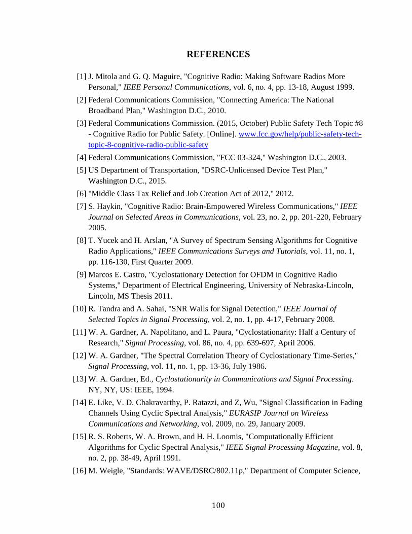
100
REFERENCES
[1] J. Mitola and G. Q. Maguire, "Cognitive Radio: Making Software Radios More Personal," IEEE Personal Communications, vol. 6, no. 4, pp. 13-18, August 1999.
[2] Federal Communications Commission, "Connecting America: The National Broadband Plan," Washington D.C., 2010.
[3] Federal Communications Commission. (2015, October) Public Safety Tech Topic #8 - Cognitive Radio for Public Safety. [Online]. www.fcc.gov/help/public-safety-tech-topic-8-cognitive-radio-public-safety
[4] Federal Communications Commission, "FCC 03-324," Washington D.C., 2003.
[5] US Department of Transportation, "DSRC-Unlicensed Device Test Plan," Washington D.C., 2015.
[6] "Middle Class Tax Relief and Job Creation Act of 2012," 2012.
[7] S. Haykin, "Cognitive Radio: Brain-Empowered Wireless Communications," IEEE Journal on Selected Areas in Communications, vol. 23, no. 2, pp. 201-220, February 2005.
[8] T. Yucek and H. Arslan, "A Survey of Spectrum Sensing Algorithms for Cognitive Radio Applications," IEEE Communications Surveys and Tutorials, vol. 11, no. 1, pp. 116-130, First Quarter 2009.
[9] Marcos E. Castro, "Cyclostationary Detection for OFDM in Cognitive Radio Systems," Department of Electrical Engineering, University of Nebraska-Lincoln, Lincoln, MS Thesis 2011.
[10] R. Tandra and A. Sahai, "SNR Walls for Signal Detection," IEEE Journal of Selected Topics in Signal Processing, vol. 2, no. 1, pp. 4-17, February 2008.
[11] W. A. Gardner, A. Napolitano, and L. Paura, "Cyclostationarity: Half a Century of Research," Signal Processing, vol. 86, no. 4, pp. 639-697, April 2006.
[12] W. A. Gardner, "The Spectral Correlation Theory of Cyclostationary Time-Series," Signal Processing, vol. 11, no. 1, pp. 13-36, July 1986.
[13] W. A. Gardner, Ed., Cyclostationarity in Communications and Signal Processing. NY, NY, US: IEEE, 1994.
[14] E. Like, V. D. Chakravarthy, P. Ratazzi, and Z, Wu, "Signal Classification in Fading Channels Using Cyclic Spectral Analysis," EURASIP Journal on Wireless Communications and Networking, vol. 2009, no. 29, January 2009.
[15] R. S. Roberts, W. A. Brown, and H. H. Loomis, "Computationally Efficient Algorithms for Cyclic Spectral Analysis," IEEE Signal Processing Magazine, vol. 8, no. 2, pp. 38-49, April 1991.
[16] M. Weigle, "Standards: WAVE/DSRC/802.11p," Department of Computer Science,
101
Old Dominion University, 2008.
[17] ASTM International, "Standard Specification for Telecommunications and Information Exchange Between Roadside and Vehicle Systems-5 GHz Band Dedicated Short Range Communications (DSRC) Medium Access Control (MAC) and Phyiscal Layer (PHY) Specifications," ASTM International, West Conshohocken, ASTM E2213-03, 2010.
[18] A. M. Abdelgader and W. Lenan, "The Physical Layer of the IEEE 802.11p WAVE Communication Standard: The Specification and Challenges," in Proceedings of the World Congress on Engineering and Computer Science 2014, vol. 2, San Francisco, 2014.
[19] S. R. Schnur, "Identification and Classification of OFDM Based Signals Using Preamble Correlation and Cyclostationary Feature Extraction," Department of Electrical and Computer Engineering, Naval Postgraduate School, Monterey, MS Thesis 2009.
[20] Tektronix. (2013, November) Wi-Fi: Overview of the 802.11 Physical Layer and Transmitter Measurements. Application Note.
[21] IEEE Computer Society, "Part 11: Wireless LAN Medium Access Control (MAC) and Physical Layer (PHY) Specification," IEEE, New York, Std 802.11, 2012.
[22] P. D. Sutton, K. E. Nolan, and L. E. Doyle, "Cyclostationary Signatures in Practical Cognitive Radio Applications," IEEE Journal on Selected Areas in Communications, vol. 26, no. 1, pp. 13-24, January 2008.
[23] D. Vucic, M. Obradovic, and D. Obradovic, "Spectral Correlation of OFDM Signals Related to Their PLC Applications," in 6th International Symposium on Power-Line Communications and Its Applications, 2002.
[24] A. Dandawate and G. Giannakis, "Statistical Tests for Presence of Cyclostationarity," IEEE Transactions on Signal Processing, vol. 42, no. 9, pp. 2355-2369, September 1994.
[25] V. Turunen, M. Kosunen, M. Vaarakangas, and J. Ryynanen, "Correlation-Based Detection of OFDM Signals in the Angular Domain," IEEE Transactions on Vehicular Technology, vol. 61, no. 3, pp. 951-958, March 2012.
[26] J. Lunden, S. A. Kassam, and V. Koivunen, "Robust Nonparametric Cyclic Correlation-Based Spectrum Sensing for Cognitive Radio," IEEE Transactions on Signal Processing, vol. 58, no. 1, pp. 38-52, January 2010.
[27] V. Turunen, M. Kosunen, V. Koivunen, and J. Ryynanen, "Dual-Lag Correlation-Based Feature Detector of OFDM Signals with Cyclic Phase Compensation," in COCORA 2012: The Second International Conference on Advances in Cognitive Radio, Chamonix, 2012.
[28] Litepoint, Practical Manufacturing Testing of 802.11 OFDM Wireless Devices,

102
2012.
[29] J.M. Lee, M.S. Woo, and S.G. Min, "Performance Analysis of WAVE Control Channels for Public Safety Services in VANETs," International Journal of Computer and Communications Engineering, vol. 2, no. 5, September 2013.
[30] J. E. Volder, "The CORDIC Trigonometric Computing Technique," IRE Transactions on Electronic Computers, vol. EC-8, no. 3, pp. 330-334, September 1959.
[31] R. Andraka, "A Survey of CORDIC Algorithms for FPGA Based Computers," Andraka Consulting Group, Inc., North Kingstown, 1999.
[32] Altera. (2011, July) Advanced Synthesis Cookbook. Document.