FPGA-Based Implementation of QR Decomposition … Implementation of QR Decomposition by ... A Thesis Presented in Partial Fulfillment ... is the estimated p by p covariance matrix

FPGA-Based Implementation of QR Decomposition

by

Hanguang Yu

A Thesis Presented in Partial Fulfillment

of the Requirements for the Degree

Master of Science

Approved April 2014 by the

Graduate Supervisory Committee:

Daniel Bliss, Chair

Lei Ying

Chaitali Chakrabarti

ARIZONA STATE UNIVERSITY

May 2014

i

ABSTRACT

This thesis report aims at introducing the background of QR decomposition and its

application. QR decomposition using Givens rotations is a efficient method to prevent

directly matrix inverse in solving least square minimization problem, which is a typical

approach for weight calculation in adaptive beamforming. Furthermore, this thesis

introduces Givens rotations algorithm and two general VLSI (very large scale integrated

circuit) architectures namely triangular systolic array and linear systolic array for

numerically QR decomposition. To fulfill the goal, a 4 input channels triangular systolic

array with 16bits fixed-point format and a 5 input channels linear systolic array are

implemented on FPGA (Field programmable gate array). The final result shows that the

estimated clock frequencies of 65 MHz and 135 MHz on post-place and route static

timing report could be achieved using Xilinx Virtex 6 xc6vlx240t chip. Meanwhile, this

report proposes a new method to test the dynamic range of QR-D. The dynamic range of

the both architectures can be achieved around 110dB.

ii

ACKNOWLEGEMENTS

I first would like to acknowledge my graduate advisor Dr. Daniel W. Bliss. His

guidance and assistance on my thesis and research was invaluable. His wisdom, kindness

and patient impress me. Over the two years, he has shared his ideas, time, and resource

graciously with me. For this, I am most appreciative.

I would like to acknowledge Dr. Chaitali Chakrabarti for providing me the FPGA

development board and give me advising on my QR-D processor design. I also like to

acknowledge Dr. Lei Ying to provide me funding source on the research on USRP. For

their contribution, I am most grateful.

Additionally, I would like to acknowledge my friends, the members of Dr. Bliss’s

laboratory, for helping on practicing my thesis defense and courses learning over these

two years. I also would like to acknowledge Mr. Min Yang, the student of Dr. Chaitali

Chakrabarti, and Mr. Zhaorui Wang, my laboratory colleague, for their generous help on

details in my thesis.

Finally, I would like to acknowledge my parents for supporting me studying in USA

and encouraging me through the hard time. I would like to follow the family traditions

that make contributions on research and serve my motherland.

iii

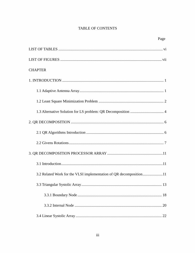
TABLE OF CONTENTS

Page

LIST OF TABLES ............................................................................................................. vi

LIST OF FIGURES .......................................................................................................... vii

CHAPTER

1. INTRODUCTION .......................................................................................................... 1

Adaptive Antenna Array ........................................................................................ 1 1.1

Least Square Minimization Problem .................................................................... 2 1.2

Alternative Solution for LS problem: QR Decomposition ................................... 4 1.3

2. QR DECOMPOSITION ................................................................................................. 6

QR Algorithms Introduction ................................................................................. 6 2.1

Givens Rotations ................................................................................................... 7 2.2

3. QR DECOMPOSITION PROCESSOR ARRAY ..........................................................11

Introduction ..........................................................................................................11 3.1

Related Work for the VLSI implementation of QR decomposition .....................11 3.2

Triangular Systolic Array .................................................................................... 13 3.3

3.3.1 Boundary Node ........................................................................................ 18

3.3.2 Internal Node ........................................................................................... 20

Linear Systolic Array .......................................................................................... 22 3.4

iv

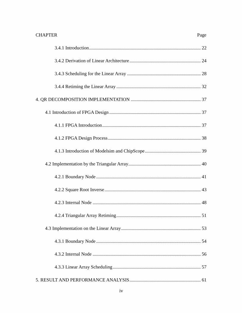
CHAPTER Page

3.4.1 Introduction .............................................................................................. 22

3.4.2 Derivation of Linear Architecture ............................................................ 24

3.4.3 Scheduling for the Linear Array .............................................................. 28

3.4.4 Retiming the Linear Array ....................................................................... 32

4. QR DECOMPOSITION IMPLEMENTATION ........................................................... 37

Introduction of FPGA Design ............................................................................. 37 4.1

4.1.1 FPGA Introduction ................................................................................... 37

4.1.2 FPGA Design Process .............................................................................. 38

4.1.3 Introduction of Modelsim and ChipScope ............................................... 39

Implementation by the Triangular Array............................................................. 40 4.2

4.2.1 Boundary Node ........................................................................................ 41

4.2.2 Square Root Inverse ................................................................................. 43

4.2.3 Internal Node ........................................................................................... 48

4.2.4 Triangular Array Retiming ....................................................................... 51

Implementation on the Linear Array ................................................................... 53 4.3

4.3.1 Boundary Node ........................................................................................ 54

4.3.2 Internal Node ........................................................................................... 56

4.3.3 Linear Array Scheduling .......................................................................... 57

5. RESULT AND PERFORMANCE ANALYSIS ............................................................ 61

v

CHAPTER Page

Result Analysis on Triangular Array ................................................................... 63 5.1

Result Analysis on Linear Array ......................................................................... 69 5.2

6. CONCLUSION AND FUTURE WORK ...................................................................... 77

Conclusion .......................................................................................................... 77 6.1

Future Work ........................................................................................................ 77 6.2

6.2.1 Back-substitution ..................................................................................... 78

6.2.2 Weights Computation ............................................................................... 82

REFERENCES ................................................................................................................. 84

vi

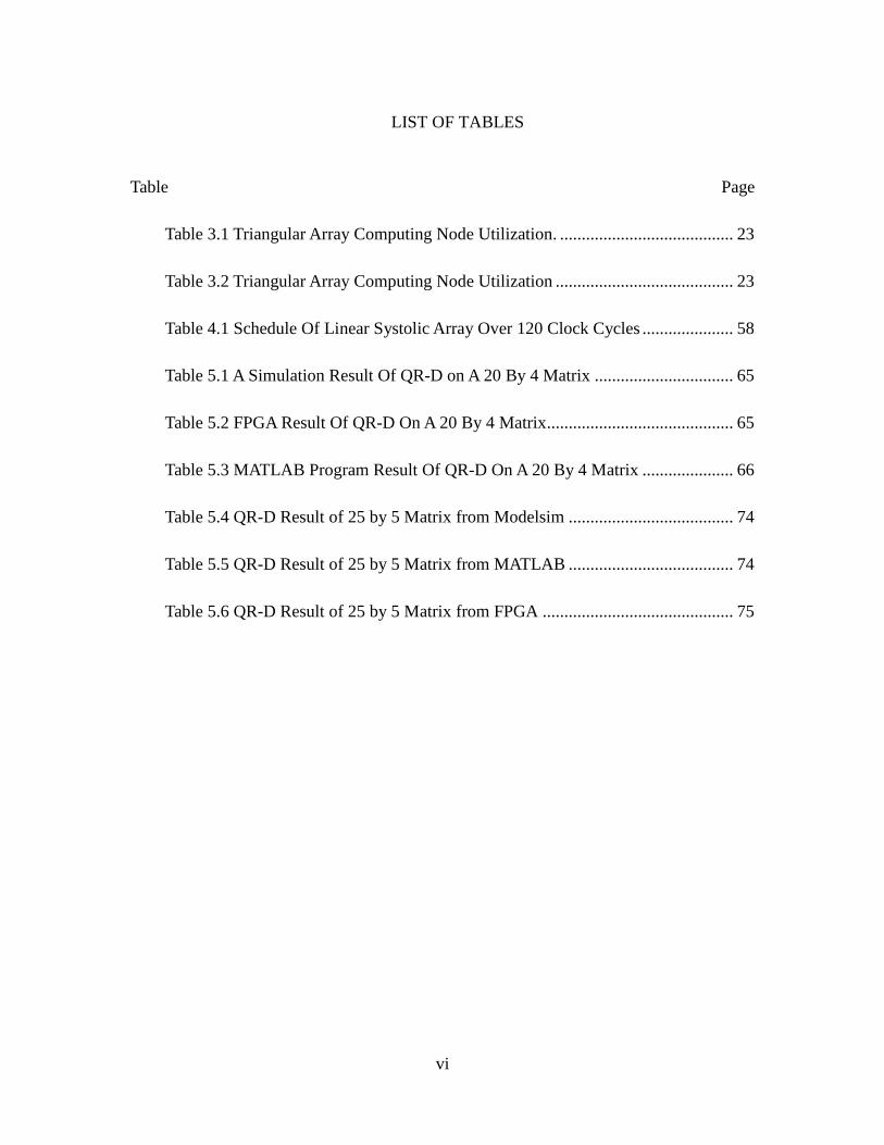
LIST OF TABLES

Table Page

Table 3.1 Triangular Array Computing Node Utilization. ........................................ 23

Table 3.2 Triangular Array Computing Node Utilization ......................................... 23

Table 4.1 Schedule Of Linear Systolic Array Over 120 Clock Cycles ..................... 58

Table 5.1 A Simulation Result Of QR-D on A 20 By 4 Matrix ................................ 65

Table 5.2 FPGA Result Of QR-D On A 20 By 4 Matrix ........................................... 65

Table 5.3 MATLAB Program Result Of QR-D On A 20 By 4 Matrix ..................... 66

Table 5.4 QR-D Result of 25 by 5 Matrix from Modelsim ...................................... 74

Table 5.5 QR-D Result of 25 by 5 Matrix from MATLAB ...................................... 74

Table 5.6 QR-D Result of 25 by 5 Matrix from FPGA ............................................ 75

vii

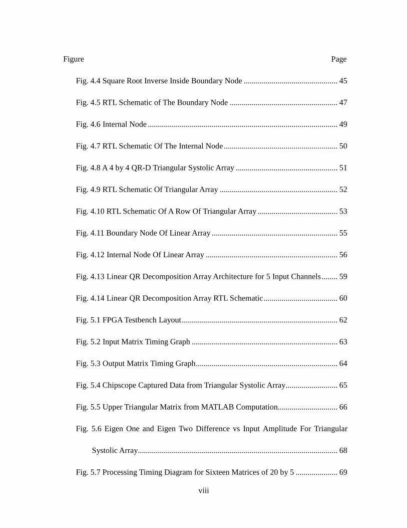
LIST OF FIGURES

Figure Page

fig. 1.1 An Adaptive Antenna Array ............................................................................ 2

Fig. 3.1 Triangular Systolic Array For QR Algorithm .............................................. 14

Fig. 3.2 Boundary Node of Triangular Systolic Array .............................................. 19

Fig. 3.3 Internal Node of Triangular Systolic Array ................................................. 21

Fig. 3.4 Triangular Systolic Array For QR Algorithm .............................................. 22

Fig. 3.5 Triangular Systolic Array For QR Algorithm (M=2) .................................. 24

Fig. 3.6 Array After Part B Mirroring Rotation (M=2) ............................................. 25

Fig. 3.7 Interleaving The Rectangular Array ............................................................ 26

Fig. 3.8 Interleaved Rectangular Arrays ................................................................... 27

Fig. 3.9 QR Decomposition Linear Systolic Array Architecture For 5 Channels ..... 28

Fig. 3.10 Scheduling The Array ................................................................................ 29

Fig. 3.11 Interleaved QR Iteration (M=2) ................................................................. 31

Fig. 3.12 A Example Of Retimed QR Nodes When Ln = 6 And Tqr = 5 ................... 33

Fig. 3.13 Effect Latency on The Schedule (M=2) .................................................... 34

Fig. 3.14 Retimed Scheduling for The Linear Array, Ln=6, Tqr=5 ............................ 36

Fig. 4.1 Fpga Developing Flow Graph ..................................................................... 39

Fig. 4.2 Pipelined Boundary Node ............................................................................ 42

Fig. 4.3 Polynomial Approximation To 1/Sqrt() [5] ................................................. 45

viii

Figure Page

Fig. 4.4 Square Root Inverse Inside Boundary Node ............................................... 45

Fig. 4.5 RTL Schematic of The Boundary Node ...................................................... 47

Fig. 4.6 Internal Node ............................................................................................... 49

Fig. 4.7 RTL Schematic Of The Internal Node ......................................................... 50

Fig. 4.8 A 4 by 4 QR-D Triangular Systolic Array ................................................... 51

Fig. 4.9 RTL Schematic Of Triangular Array ........................................................... 52

Fig. 4.10 RTL Schematic Of A Row Of Triangular Array ........................................ 53

Fig. 4.11 Boundary Node Of Linear Array ............................................................... 55

Fig. 4.12 Internal Node Of Linear Array .................................................................. 56

Fig. 4.13 Linear QR Decomposition Array Architecture for 5 Input Channels ........ 59

Fig. 4.14 Linear QR Decomposition Array RTL Schematic ..................................... 60

Fig. 5.1 FPGA Testbench Layout .............................................................................. 62

Fig. 5.2 Input Matrix Timing Graph ......................................................................... 63

Fig. 5.3 Output Matrix Timing Graph ....................................................................... 64

Fig. 5.4 Chipscope Captured Data from Triangular Systolic Array .......................... 65

Fig. 5.5 Upper Triangular Matrix from MATLAB Computation.............................. 66

Fig. 5.6 Eigen One and Eigen Two Difference vs Input Amplitude For Triangular

Systolic Array.................................................................................................... 68

Fig. 5.7 Processing Timing Diagram for Sixteen Matrices of 20 by 5 ..................... 69

ix

Figure Page

Fig. 5.8 Timing Diagram of A Complete QR Decompostion ................................... 71

Fig. 5.9 Result Matrix Output Procedure (A) ........................................................... 72

Fig. 5.10 Result Matrix Output Procedure (B) ......................................................... 73

Fig. 5.11 Result Matrix from Chipscope ................................................................... 74

Fig. 5.12 Result Matrix from MATLAB ................................................................... 74

Fig. 5.13 Eigen One and Eigen Two Difference vs Input Amplitude for Linear

Systolic Array.................................................................................................... 75

Fig. 6.1 Adaptive Beamforming System [13] ........................................................... 78

Fig. 6.2 “Frozen” Triangular Array [1] ..................................................................... 79

Fig. 6.3 A QR-D Of 4 Channels with Weight Flushing (Each Node Have One Clock

Cycle Delay) [1] ................................................................................................ 81

Fig. 6.4 Weights Computing Process ........................................................................ 83

1

1. INTRODUCTION

Adaptive Antenna Array 1.1

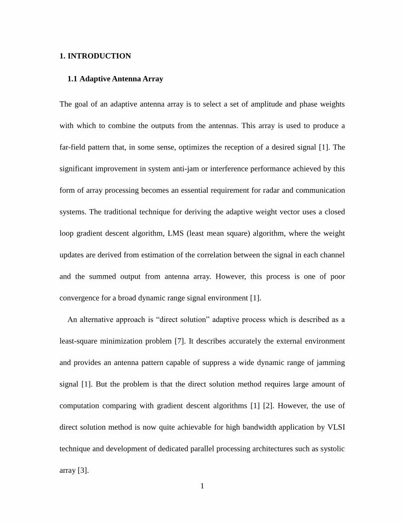
The goal of an adaptive antenna array is to select a set of amplitude and phase weights

with which to combine the outputs from the antennas. This array is used to produce a

far-field pattern that, in some sense, optimizes the reception of a desired signal [1]. The

significant improvement in system anti-jam or interference performance achieved by this

form of array processing becomes an essential requirement for radar and communication

systems. The traditional technique for deriving the adaptive weight vector uses a closed

loop gradient descent algorithm, LMS (least mean square) algorithm, where the weight

updates are derived from estimation of the correlation between the signal in each channel

and the summed output from antenna array. However, this process is one of poor

convergence for a broad dynamic range signal environment [1].

An alternative approach is “direct solution” adaptive process which is described as a

least-square minimization problem [7]. It describes accurately the external environment

and provides an antenna pattern capable of suppress a wide dynamic range of jamming

signal [1]. But the problem is that the direct solution method requires large amount of

computation comparing with gradient descent algorithms [1] [2]. However, the use of

direct solution method is now quite achievable for high bandwidth application by VLSI

technique and development of dedicated parallel processing architectures such as systolic

array [3].

2

Least Square Minimization Problem 1.2

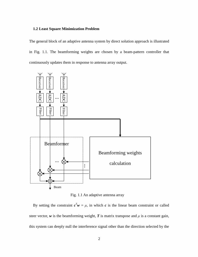
The general block of an adaptive antenna system by direct solution approach is illustrated

in Fig. 1.1. The beamforming weights are chosen by a beam-pattern controller that

continuously updates them in response to antenna array output.

By setting the constraint cTw = μ, in which c is the linear beam constraint or called

steer vector, w is the beamforming weight, T is matrix transpose and μ is a constant gain,

this system can deeply null the interference signal other than the direction selected by the

AD

C

AD

C

AD

C

Receiv

er

Receiv

er

Receiv

er

Filter

F

ilter

Filter

…

…

…

Beam

Fig. 1.1 An adaptive antenna array

Beamforming weights

calculation

Beamformer

3

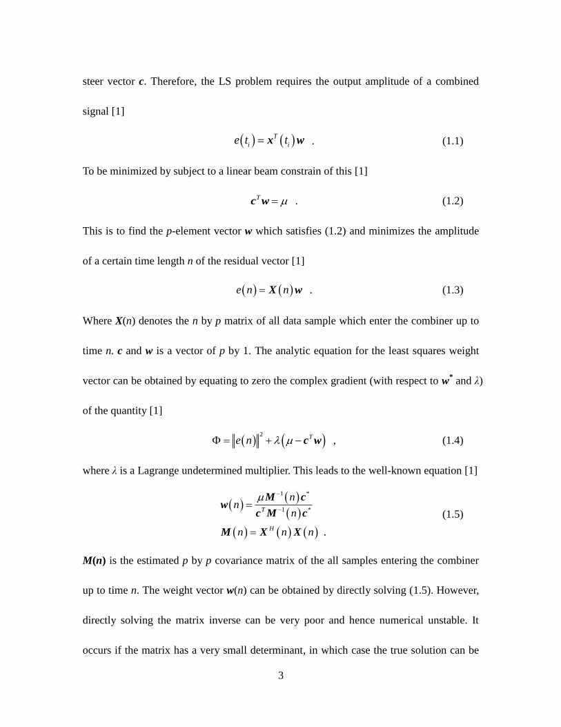
steer vector c. Therefore, the LS problem requires the output amplitude of a combined

signal [1]

T

i ie t t x w . (1.1)

To be minimized by subject to a linear beam constrain of this [1]

T c w . (1.2)

This is to find the p-element vector w which satisfies (1.2) and minimizes the amplitude

of a certain time length n of the residual vector [1]

e n n X w . (1.3)

Where X(n) denotes the n by p matrix of all data sample which enter the combiner up to

time n. c and w is a vector of p by 1. The analytic equation for the least squares weight

vector can be obtained by equating to zero the complex gradient (with respect to w* and λ)

of the quantity [1]

2 Te n c w , (1.4)

where λ is a Lagrange undetermined multiplier. This leads to the well-known equation [1]

1 *

1 *

.

T

H

nn

n

n n n

M cw

c M c

M X X

(1.5)

M(n) is the estimated p by p covariance matrix of the all samples entering the combiner

up to time n. The weight vector w(n) can be obtained by directly solving (1.5). However,

directly solving the matrix inverse can be very poor and hence numerical unstable. It

occurs if the matrix has a very small determinant, in which case the true solution can be

4

subject to large perturbations and satisfy the equation quite accurately. This will lead to

very complicated circuit architecture for numerical computation. This is definitely not

suitable for VLSI implementation.

Alternative Solution for LS problem: QR Decomposition 1.3

An alternative approach to the least-squares estimation problem which is the most

suitable for the numerical sense is the orthogonal triangularization [1]. This method is

known as QR decomposition [4].

An n by p data matrix X(n) can be decomposed as [1]

n n nX Q R . (1.6)

where R(n) is a n by p upper triangular matrix and Q(n) is a unitary matrix of n by n. p is

the number of antenna elements and n is the number of samples.

Applying QR decomposition to (2.5), we can get [1]

1*

1 *

H

Tn

n

QR QR cw

c M c . (1.7)

The denominator is some constant number. Thus, we can ignore the denominator and μ

since they will not change the phase of the weights.

1

*H

w R R c . (1.8)

Since the matrix R(n) is upper triangular, (1.8) can be easily solved. The weight vector

w(n) may be derived simply by double back-substitution [5].

Of course, it does not matter to use which of the algorithm for matrix triangularization

5

when the LS problem is not constrained by speed and throughput, for example simply

using computer to do QR decomposition. However, when the application scenario is an

adaptive antennas array, for example in MIMO (multiple input multiple output)

communication system or phased array radar, there is no choice but the only method to

use a proper VLSI (very large scale circuit) system to fulfill the application criteria.

6

2. QR DECOMPOSITION

QR Algorithms Introduction 2.1

The QR decomposition of a m-by-n matrix A is given be [4]

A QR , (2.1)

where m mQ is orthogonal matrix and m nR is upper triangular matrix. If m > n,

R consists of an n by n right upper triangular matrix and a (m-n) by n zeroes matrix below

the triangular matrix.

For solving the QR decomposition, there are several different methods available to use

including Gram-Schmidt algorithm [4], Householder transformation algorithm [4] and

Givens rotations algorithm [4] [6]. Gram-Schmidt algorithm utilizes the Gram-Schmidt

orthogonalization to compute the upper triangular matrix. Householder transformation

algorithm is to eliminate certain lower elements on each row by multiplier each

Householder matrices. Givens rotations is to get compute a rotation factor from the

adjacent elements to eliminate the lower element in each rotation matrix. This Givens

rotations triangularization processing is recursively updated as each new row of data

entering the array. The recursive updating only involves two adjacent rows from the input

data matrix which is particularly suitable for systolic array structure of VLSI

implementation.

7

Givens Rotations 2.2

A complex Givens rotations [6] is presented by the following elementary transformation

of this form

*1

0

n

n

r yc s

xs c

, (2.2)

where n presents the different time. rn-1 arrives earlier than xn one unit time. We want to

eliminate the lower element xn. Thus the rotation coefficients c and s need to satisfy the

following equations

2 2

1n n nr x r , (2.3)

1

**

1 1

n n

n n

n n

n n

r xc s

r r

cx cxs s

r r

. (2.4)

Bring (2.5) and (2.6) back to (2.7), we can find

1 1

1

2 ** 1

1

1 1 0nn n n n n

n

n n nn n n

n n

cxsr cx r cx cx

r

r x xcr s x r y

r r

. (2.8)

Here c and s stands for cosine and sine parameters. |c|2+|s|

2=1.

Therefore a process of such elimination operation can be used to triangularize the matrix

in a recursive manner. Assuming a 4 by 4 matrix, we multiply a rotation matrix where the

elementary matrix moves along with column direction as equation (2.11). First, we

calculate the value of c1 and s1 from x31 and x41 by equation (2.9) and (2.10) with rn-1

8

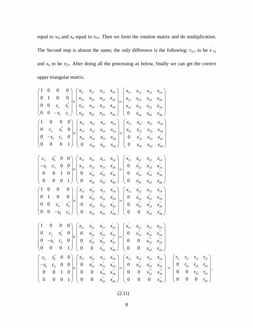
equal to x41 and xn equal to x31. Then we form the rotation matrix and do multiplication.

The Second step is almost the same; the only difference is the following: rn-1 to be x’31

and xn to be x21. After doing all the processing as below, finally we can get the correct

upper triangular matrix.

11 12 13 14 11 12 13 14

21 22 23 24 21 22 23 24

* ' ' ' '31 32 33 341 1 31 32 33 34

' ' '41 42 43 441 1 42 43 44

11

*

2 2

2 2

1 0 0 0

0 1 0 0

0 0

0 0 0

1 0 0 0

0 0

0 0

0 0 0 1

x x x x x x x x

x x x x x x x x

x x x xc s x x x x

x x x xs c x x x

x x

c s

s c

12 13 14 11 12 13 14

' ' ' '

21 22 23 24 21 22 23 24

' ' ' ' '' '' ''

31 32 33 34 32 33 34

' ' ' ' ' '

42 43 44 42 43 44

0

0 0

x x x x x x

x x x x x x x x

x x x x x x x

x x x x x x

' ' ' '*

11 12 13 14 11 12 13 143 3

' ' ' ' '' '' ''

21 22 23 24 22 23 243 3

'' '' '' '' '' ''

32 33 34 32 33 34

' ' ' ' ' '

42 43 44 42 43 44

*

4 4

4 4

0 0

00 0

0 00 0 1 0

0 00 0 0 1

1 0 0 0

0 1 0 0

0 0

0 0

x x x x x x x xc s

x x x x x x xs c

x x x x x x

x x x x x x

c s

s c

' ' ' ' ' ' ' '

11 12 13 14 11 12 13 14

'' '' '' '' '' ''

22 23 24 22 23 24

'' '' '' ''' ''' '''

32 33 34 32 33 34

' ' ' '' ''

42 43 44 43 44

0 0

0 0

0 0 0

x x x x x x x x

x x x x x x

x x x x x x

x x x x x

' ' ' ' ' ' ' '

11 12 13 14 11 12 13 14

* '' '' '' ''' ''' '''

5 5 22 23 24 22 23 24

''' ''' ''' '''' ''''

5 5 32 33 34 33 34

'' '' '' ''

43 44 43 44

*

6 6

6 6

1 0 0 0

0 0 0 0

0 0 0 0 0

0 0 0 1 0 0 0 0

0 0

0 0

x x x x x x x x

c s x x x x x x

s c x x x x x

x x x x

c s

s c

' ' ' ' ' ' ' '11 12 13 1411 12 13 14 11 12 13 14

''' ''' ''' ''' ''' '''22 23 2422 23 24 22 23 24

'''' '''' ''''' '''''3333 34 33 34

'' '' '''

43 44 44

00 0

0 00 0 0 00 0 1 0

0 0 0 0 00 0 0 1

r r r rx x x x x x x x

r r rx x x x x x

r rx x x x

x x x

34

44

.

0 0 0 r

(2.11)

9

From the above process, we can see the rotation values come from the adjacent two

elements in the same column, for example c1 and s1 are computed from x31 and x41. Then

c1 and s1 will involve the multiplication on matrix32 33 34

42 43 44

x x x

x x x

. Thus, we can

conclude there are two kind of computation. First one is to get c and s values and second

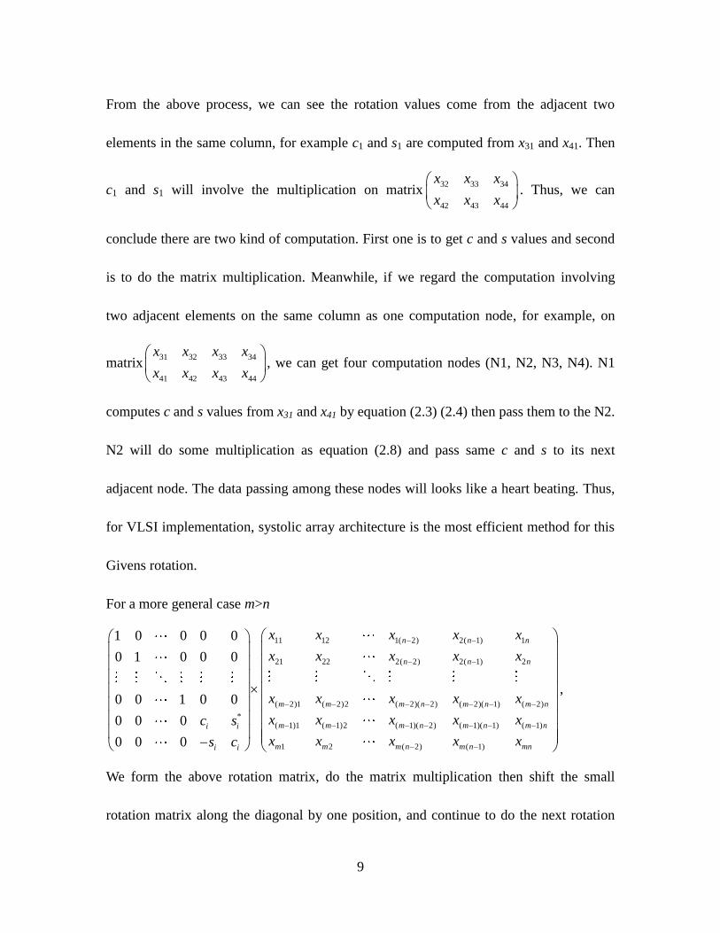
is to do the matrix multiplication. Meanwhile, if we regard the computation involving

two adjacent elements on the same column as one computation node, for example, on

matrix31 32 33 34

41 42 43 44

x x x x

x x x x

, we can get four computation nodes (N1, N2, N3, N4). N1

computes c and s values from x31 and x41 by equation (2.3) (2.4) then pass them to the N2.

N2 will do some multiplication as equation (2.8) and pass same c and s to its next

adjacent node. The data passing among these nodes will looks like a heart beating. Thus,

for VLSI implementation, systolic array architecture is the most efficient method for this

Givens rotation.

For a more general case m>n

11 12 1( 2) 2( 1) 1

21 22 2( 2) 2( 1) 2

( 2)1 ( 2)2 ( 2)( 2) ( 2)( 1) ( 2)

*( 1)1 ( 1)2 ( 1)( 2) ( 1)( 1) (

1 0 0 0 0

0 1 0 0 0

0 0 1 0 0

0 0 0

0 0 0

n n n

n n n

m m m n m n m n

m m m n m n mi i

i i

x x x x x

x x x x x

x x x x x

x x x x xc s

s c

1)

1 2 ( 2) ( 1)

n

m m m n m n mnx x x x x

,

We form the above rotation matrix, do the matrix multiplication then shift the small

rotation matrix along the diagonal by one position, and continue to do the next rotation

10

computation as the followings

11 12 1( 2) 2( 1) 1

21 22 2( 2) 2( 1) 2

*( 2)1 ( 2)2 ( 2)( 2) ( 2)( 1) ( 2)2 2

( 1)1 ( 1)2 ( 1)( 2) ( 1)( 1) (2 2

1 0 0 0 0

0 1 0 0 0

0 0 0

0 0 0

0 0 0 0 1

n n n

n n n

m m m n m n m n

m m m n m n m

x x x x x

x x x x x

x x x x xc s

x x x x xs c

1)

2 ( 2) ( 1)0

n

m m n m n mnx x x x

.

Until the small rotation matrix reaches the left top as below

*11 12 1( 2) 2( 1) 1

21 22 2( 2) 2( 1) 2

' ' ' '

( 2)2 ( 2)( 2) ( 2)( 1) ( 2)

' ' ' '

( 1)2 ( 1)( 2) ( 1)( 1) ( 1)

0 0 0

0 0 0

00 0 1 0 0

00 0 0 1 0

0 0 0 0 1

n n nm m

n n nm m

m m n m n m n

m m n m n m

x x x x xc s

x x x x xs c

x x x x

x x x x

' ' ' '

2 ( 2) ( 1)0

n

m m n m n mnx x x x

,

Put the small rotation matrix back to the right bottom as below, and start the new round of

rotations to eliminate the elements on the second column.

' ' ' ' '

11 12 1( 2) 2( 1) 1

' ' ' '

22 2( 2) 2( 1) 2

' ' ' '

( 2)2 ( 2)( 2) ( 2)( 1) ( 2)

* ' ' '

1 1 ( 1)2 ( 1)( 2) ( 1

1 1

1 0 0 0 0

0 1 0 0 0 0

0 0 1 0 0 0

0 0 0 0

0 0 0

n n n

n n n

m m n m n m n

m m m m n m

m m

x x x x x

x x x x

x x x x

c s x x x

s c

'

)( 1) ( 1)

' ' ' '

2 ( 2) ( 1)0

n m n

m m n m n mn

x

x x x x

.

Of course, the c and s are different on each rotation.

11

3. QR DECOMPOSITION PROCESSOR ARRAY

Introduction 3.1

In order to fulfill the high speed and high throughput requirement for the scenario of

antenna array beamforming, a highly parallel systolic array can be mapped from the

Givens rotations algorithm. Input the matrix, need triangularization, to the processing

array. Then it will output the each element of the triangular matrix or store each element

in corresponding nodes and continue for beamforming weight computation. VLSI is the

best choice to fulfill the goal. However, it is impossible for all these QRD algorithms to

be implemented into a VLSI system. The best choice is to use Givens rotations [1][8][9].

Using Givens rotations, QRD can be represented as a highly parallel array consists of

computation nodes. This leads to systolic array architecture.

Related Work for the VLSI implementation of QR decomposition 3.2

The earliest work of VLSI architecture of QRD is proposed by H. T Kung and W. M

Gentleman in 1981[10]. Two years later, in 1983 J. G. McWhirter [9] also proposed the

similar method of matrix triangulation for solving least squares minimization using

systolic array. But McWhirter’s work has the antenna array as the background and also

proposed the proper method for compute beamforming weight. The following published

works are all based on their fundamental architecture, which mainly focus on improving

12

computation speed and throughput. These works fall into three categories [11]. One

classic of implementation is square root free using the Squared Givens rotation algorithm

[12 W. M Gentleman 1973]. Another type of implementation is based on Logarithmic

Number system arithmetic. The last category of implementation uses CORDIC algorithm

[22 Volder 1959].

In 1999, a novel linear QR architecture was developed by R. Walke[14]. It is not the

first work to propose a linear array for least square problem. The earlier works come from

different authors, namely Yang and Bohme [24], Chen and Yao [25], Rader [26].

However, this work is quite significant different from other kinds of linear array. It is

directly mapped from the conventional triangular array ([9] McWhirter array) based on

the same recursive algorithm. Due to its easy to understand and build, more recently

public works [5][19][23] and even commercial QR-D IP cores use this linear systolic

array. The linear systolic array helps to save huge computation nodes and improve the

utilization of each computation node to 100 percent compared with the conventional QR

architecture [9][10].

On FPGA side, [R. Walke et al.] first use QRD for weight computation for adaptive

beamforming application. A Squared Givens Rotation (W. M Gentleman 1973) algorithm

is used to avoid the square root operation. The follow up work [R. Walke et al. 2000] uses

the SGR algorithm and implements a linear array on Xilinx Virtex-E FPGA. A maximum

of 9 processors can fit in, achieving a clock rare of 150MHz and throughput of

13

20GFLOPS with floating point operation [13]. R. L. Walke et al also first implements a

linear array architecture [2][14] using CORDIC algorithm for rotation computing [16].

From R. Walke’s work, a 26-bits fixed-point data format is used to guarantee sufficient

interference suppression. There are also many commercial QR-D IP (Intelligence Patent)

cores using CORDIC algorithm. Altera published a QRD-RLS design based on CORDIC

core [18].

Triangular Systolic Array 3.3

This kind of systolic array for QR decomposition is proposed by H. T Kung and W. M

Gentleman [10]. J. G. McWhirter first introduces this method to the scenario of antenna

array [9].

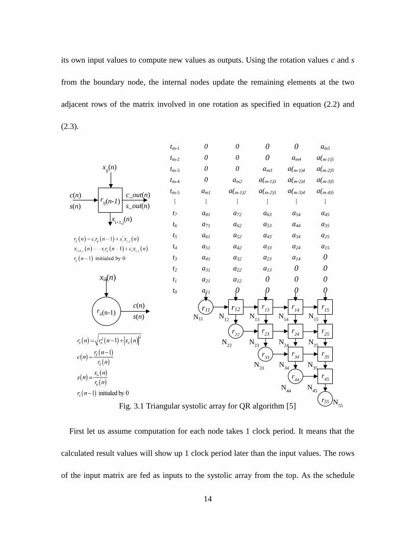
This systolic array consists of two types of computational nodes: boundary node on

diagonal of the triangular matrix and internal node off the diagonal. The boundary nodes

are used to calculate the Givens rotation that is applied over a particular row in the input

matrix. An orthogonal rotation matrix as in equation (2.2) that can eliminate one lower

triangular element of the decomposed matrix is computed in the boundary node, while the

rotation parameters c and s are output to the internal nodes. The generated rotation

parameters are sequentially broadcasted to the internal nodes in the same row as the

boundary node from left to right by a certain clock rate. The internal nodes apply this

Givens rotation parameters received from the boundary node on the same row as well as

14

its own input values to compute new values as outputs. Using the rotation values c and s

from the boundary node, the internal nodes update the remaining elements at the two

adjacent rows of the matrix involved in one rotation as specified in equation (2.2) and

(2.3).

First let us assume computation for each node takes 1 clock period. It means that the

calculated result values will show up 1 clock period later than the input values. The rows

of the input matrix are fed as inputs to the systolic array from the top. As the schedule

tm-1 0 0 0 0 am5

tm-2 0 0 0 am4 a(m-1)5

tm-3 0 0 am3 a(m-1)4 a(m-2)5

tm-4 0 am2 a(m-1)3 a(m-2)4 a(m-3)5

tm-5 am1 a(m-1)2 a(m-2)3 a(m-3)4 a(m-4)5

⁞ ⁞ ⁞ ⁞ ⁞ ⁞

t7 a81 a72 a63 a54 a45

t6 a71 a62 a53 a44 a35

t5 a61 a52 a43 a34 a25

t4 a51 a42 a33 a24 a15

t3 a41 a32 a23 a14 0

t2 a31 a22 a13 0 0

t1 a21 a12 0 0 0

t0 a11 0 0 0 0

Fig. 3.1 Triangular systolic array for QR algorithm [5]

rii(n-1)

xii(n)

c(n)

s(n)

rij(n-1)

c(n)

s(n)

c_out(n)

s_out(n)

xij(n)

xi+1,j

(n)

r11 r12 r13 r

14 r

15

r22 r

23 r

24 r

25

r33 r

34 r

35

r44 r

45

r55

N11 N12 N

13 N

14 N

15

N22 N

23 N

24 N

25

N33 N

34 N

35

N44 N

45

N55

15

graph on Fig. 3.1, after receiving the first input value a11 at t0, the boundary node N11

starts computing. The boundary node N11 will update its stored value r11 and output c and

s at the time t1. Meanwhile, internal node N12 receives c, s and a12. It will update its stored

value r12 and pass the result to the lower level node N22. It also passes the same c and s to

its right adjacent node N13 at time t2. At t2, internal node N13 receives c, s and a13. After

one clock period computation, it will update its stored value r13 and pass the result to the

lower level node N23 and the same c and s to its right adjacent node N14 at the time t3. At

t3, internal node N14 receives c, s and a14. After one clock period computation, it will

update its stored value r14 and pass the result to the lower level node N24 and the same c

and s to its right adjacent node N15 at the time t4. At t4, internal node N15 receives c, s and

a15. After one clock period computation, it will only update its stored value r15 and pass

the result to the lower level node N25 at the time t5. Right now, the computation on first

row of data matrix and updated row passing is done.

The updated data row passes to the next processing row N22 N23 N24 N25 at t2 and

finishes at t6. At the same time t2, the first boundary node continues to compute rotation

parameters from the next row data a21 and stored row data r11. Then pass the c and s value

to the internal nodes on the same row. The internal node N12 to N15 will also continue to

compute on the row data a22 to a25) and stored row data (r12 to r15), update stored row data

(r12 to r15) and output data to the row below them. In the same fashion, the boundary node

N33 will start processing until the output data arrive from the internal node N23 above it. It

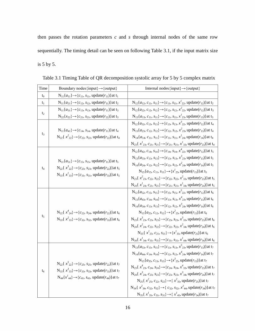
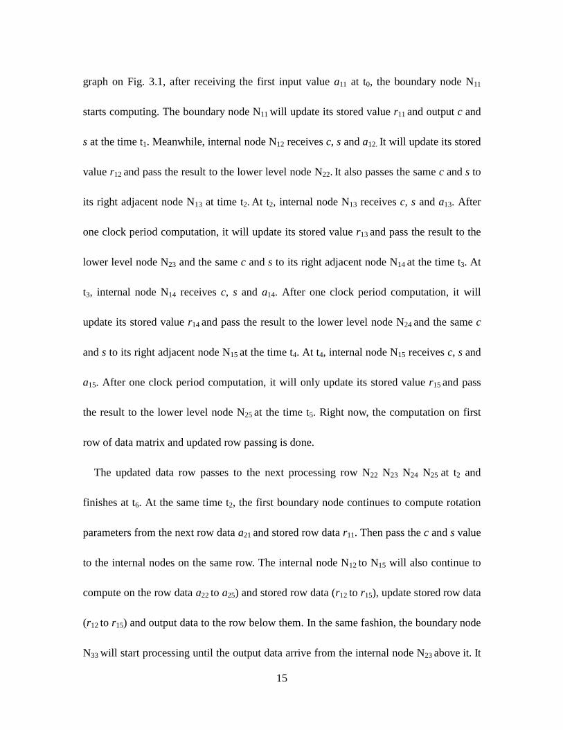
16

then passes the rotation parameters c and s through internal nodes of the same row

sequentially. The timing detail can be seen on following Table 3.1, if the input matrix size

is 5 by 5.

Table 3.1 Timing Table of QR decomposition systolic array for 5 by 5 complex matrix

Time Boundary nodes{input}→{output} Internal nodes{input}→{output}

t0 N11{a11}→{c11, s11, update(r11)}at t1

t1 N11{a21}→{c12, s12, update(r11)}at t2 N12{a12, c11, s11}→{c11, s11, x1

22, update(r12)}at t2

t2

N11{a31}→{c13, s13, update(r11)}at t3

N22{x22}→{c21, s21, update(r22)}at t3

N12{a22, c12, s12}→{c12, s12, x2


N13{a13, c11, s11}→{c11, s11, x123, update(r13)}at t3

t3

N11{a41}→{c14, s14, update(r11)}at t4

N22{ x2

22}→{c22, s22, update(r22)}at t4

N12{a32, c13, s13}→{c13, s13, x3


N13{a23, c12, s12}→{c12, s12, x2


N14{a14, c11, s11}→{c11, s11, x124, update(r14)}at t4

N23{ x1

23, c21, s21}→{c21, s21, x133, update(r23)}at t4

t4

N11{a51}→{c15, s15, update(r11)}at t5

N22{ x3

22}→{c23, s23, update(r22)}at t5

N33{ x1

33}→{c31, s31, update(r33)}at t5

N12{a42, c14, s14}→{c14, s14, x4


N13{a33, c13, s13}→{c13, s13, x3


N14{a24, c12, s12}→{c12, s12, x2


N15{a15, c11, s11}→{x1


N23{ x2


N24{ x1


t5

N22{ x4

24}→{c22, s24, update(r22)}at t6

N33{ x2

33}→{c32, s32, update(r33)}at t6

N12{a52, c15, s15}→{c15, s15, x5


N13{a43, c14, s14}→{c13, s13, x4


N14{a34, c13, s13}→{c12, s12, x3


N15{a25, c12, s12}→{x225, update(r15)}at t6

N23{ x3


N24{ x2


N25{ x1

25, c21, s21}→{x135, update(r25)}at t6

N34{ x1


t6

N22{ x5

22}→{c25, s25, update(r22)}at t7

N33{ x3

33}→{c33, s33, update(r33)}at t7

N44{x144}→{c41, s41, update(r44)}at t7

N13{a53, c15, s15}→{c13, s13, x5


N14{a44, c14, s14}→{c12, s12, x4



N23{ x4


N24{ x3


N25{ x225, c22, s22}→{ x


N34{ x234, c32, s32}→{ c32, s32, x


N35{ x135, c31, s31}→{ x


17

t7

N33{ x4

33}→{c34, s34, update(r33)}at t8

N44{x244}→{c42, s42, update(r44)}at t8

N14{a44, c15, s15}→{c12, s12, x5



N23{ x5


N24{ x4


N25{ x3

25, c23, s23}→{x335, update(r25)}at t8

N34{ x3


N35{ x2

35, c32, s32}→{x245, update(r34)}at t8

N45{ x1

45, c41, s41}→{x155, update(r45)}at t8

t8

N33{ x5

33}→{c35, s35, update(r33)}at t9

N44{x344}→{c43, s43, update(r44)}at t9

N55{ x1

55}→{c51, s51, update(r55)}at t9


N24{ x5


N25{ x425, c24, s24}→{ x


N34{ x434, c34, s34}→{ c34, s34, x


N35{ x335, c33, s33}→{ x


N45{ x2

45, c42, s42}→{x255, update(r45)}at t9

t9

N44{x4

44}→{c44, s44, update(r44)}at t10

N55{ x255}→{c52, s52, update(r55)}at t10

N25{ x525, c25, s25}→{ x


N34{ x534, c35, s35}→{ c35, s35, x


N35{ x435, c34, s34}→{ x


N45{ x345, c43, s43}→{x


t10

N44{x544}→{c45, s45, update(r44)}at t11

N55{ x3

55}→{c53, s53, update(r55)}at t11

N35{ x535, c35, s35}→{ x


N45{ x4

45, c44, s44}→{x455, update(r45)}at t11

t11 N55{ x455}→{c54, s54, update(r55)}at t12 N45{ x

545, c45, s45}→{x


t12 N55{ x555}→{c55, s55, update(r55)}at t13

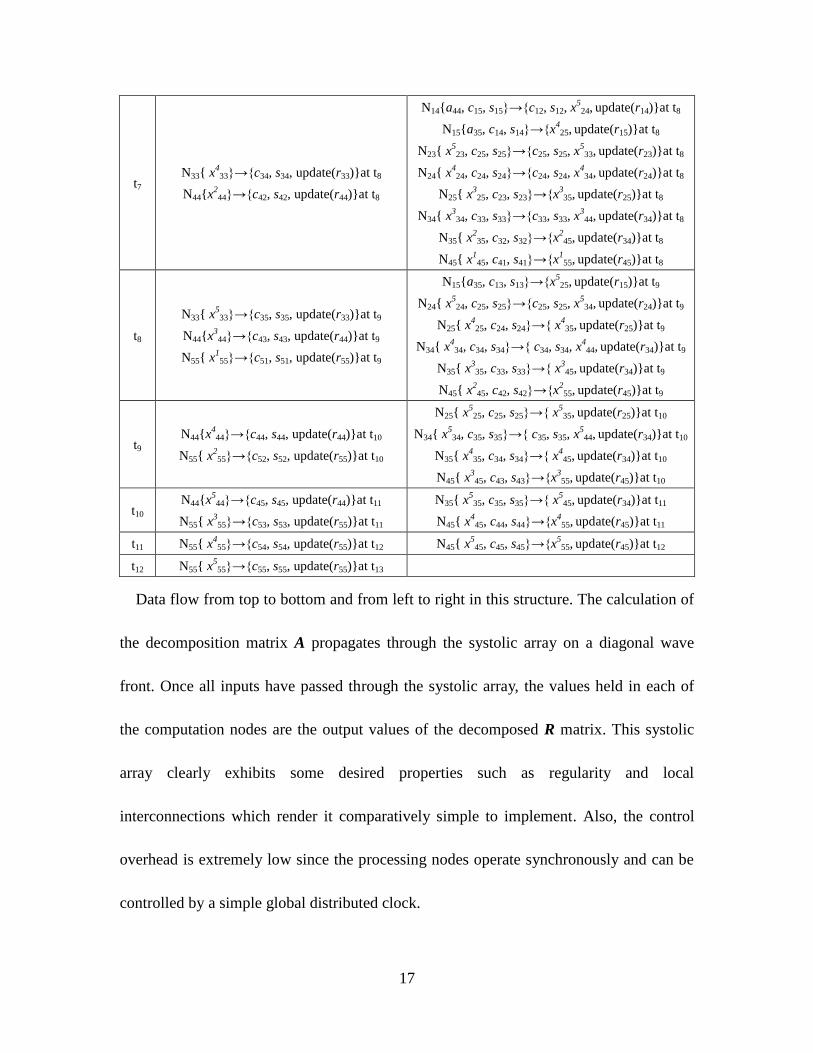
Data flow from top to bottom and from left to right in this structure. The calculation of

the decomposition matrix A propagates through the systolic array on a diagonal wave

front. Once all inputs have passed through the systolic array, the values held in each of

the computation nodes are the output values of the decomposed R matrix. This systolic

array clearly exhibits some desired properties such as regularity and local

interconnections which render it comparatively simple to implement. Also, the control

overhead is extremely low since the processing nodes operate synchronously and can be

controlled by a simple global distributed clock.

18

On the original J. G. McWhirter’s work, there is only one clock cycle for each

computing node. Apparently, it will be very slow since all the commutating operations

inside each node have to be done in 1 clock cycle. In this case, the 1 clock cycle period

should be very long to meet the time consumption of the critical path inside each node.

Therefore, the pipelines can be introduced into each computation node. It will shorten the

critical path length and increase clock speed significantly. However, the thing needed to

focus is that a proper retiming strategy has to be chosen for nodes interconnection.

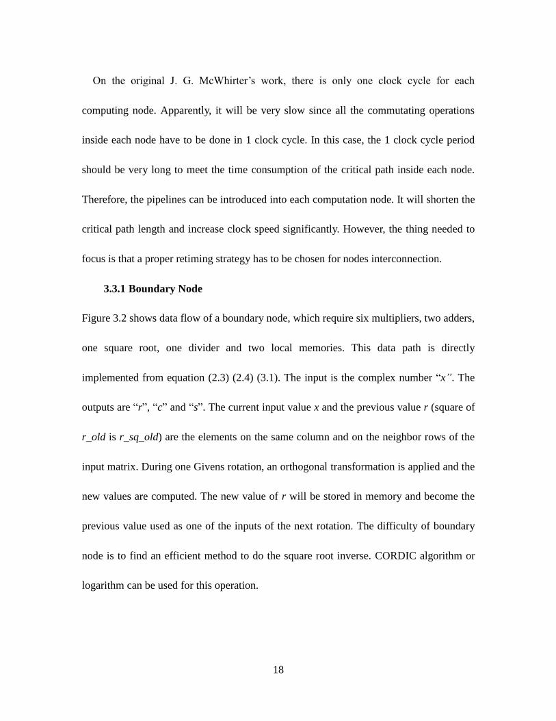
3.3.1 Boundary Node

Figure 3.2 shows data flow of a boundary node, which require six multipliers, two adders,

one square root, one divider and two local memories. This data path is directly

implemented from equation (2.3) (2.4) (3.1). The input is the complex number “x”. The

outputs are “r”, “c” and “s”. The current input value x and the previous value r (square of

r_old is r_sq_old) are the elements on the same column and on the neighbor rows of the

input matrix. During one Givens rotation, an orthogonal transformation is applied and the

new values are computed. The new value of r will be stored in memory and become the

previous value used as one of the inputs of the next rotation. The difficulty of boundary

node is to find an efficient method to do the square root inverse. CORDIC algorithm or

logarithm can be used for this operation.

19

22 1

1

ii ii ii

ii

ii

ii

ii

r n r n x n

r nc n

r n

x ns n

r n

. (3.1)

Fig. 3.2 Boundary node of triangular systolic array [5]

x_im

Square root

divider

Delay

Delay

x_real x_real x_im x_im

r_sq_old

r_sq

r

r_old

1/r

x_real

c s_real s_im

20

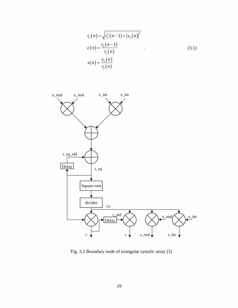
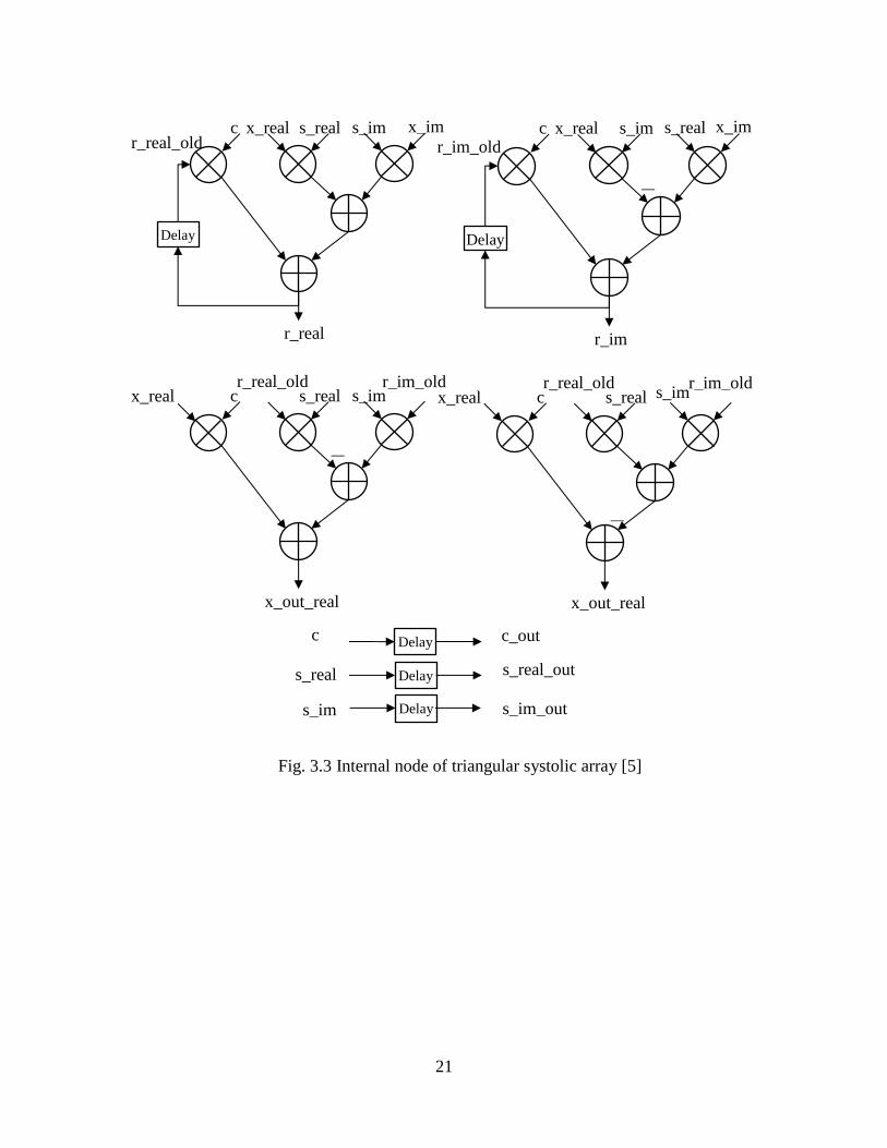
3.3.2 Internal Node

Compared with the boundary node, internal node is much simpler. It requires twelve

multipliers, five adders, three subtractors and two local memories. It is directly

implemented from equation (2.8) (3.2) in Fig. 3.3. The inputs are rotation parameters c, s

whereas x is the matrix data input. Outputs are r_real, r_im, x_out_real and x_out_im.

Another two inputs r_real_old and r_im_old are initialed by zero but updated when the

new values are input into the internal node. The previous r_old value and current input x

are the elements on the same column and on the neighbor rows of the input matrix. The

internal node applies the orthogonal transform to the input value and previous value, and

calculates two new complex numbers.

*

,

1, ,

1

1

ij i ij i i j

i j i ij i i j

r n c r n s x n

x n s r n c x n

(3.2)

21

Fig. 3.3 Internal node of triangular systolic array [5]

Delay

c x_real s_real s_im x_im

r_real

r_real_old

Delay

c x_real s_im s_real x_im

r_im

r_im_old

c r_real_old

s_real s_imr_im_old

x_out_real

x_real

c r_real_old

s_real s_im

m

r_im_old

x_out_real

x_real

c

s_real

s_im

Delay

Delay

Delay

c_out

s_real_out

s_im_out

—

—

—

22

Linear Systolic Array 3.4

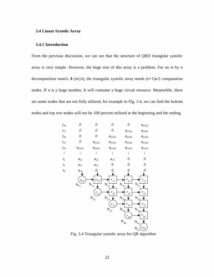
3.4.1 Introduction

From the previous discussion, we can see that the structure of QRD triangular systolic

array is very simple. However, the huge size of this array is a problem. For an m by n

decomposition matrix A (m≥n), the triangular systolic array needs (n+1)n/2 computation

nodes. If n is a large number, It will consume a huge circuit resource. Meanwhile, there

are some nodes that are not fully utilized, for example in Fig. 3.4, we can find the bottom

nodes and top row nodes will not be 100 percent utilized at the beginning and the ending.

t28 0 0 0 0 a(25)5

t27 0 0 0 a(25)4 a(24)5

t26 0 0 a(25)3 a(24)4 a(23)5

t25 0 a(25)2 a(24)3 a(23)4 a(22)5

t24 a(25)1 a(24)2 a(23)3 a(22)4 a(21)5

⁞ ⁞ ⁞ ⁞ ⁞ ⁞

t2 a31 a22 a13 0 0

t1 a21 a12 0 0 0

t0 a11 0 0 0 0

Fig. 3.4 Triangular systolic array for QR algorithm

r11 r12 r13 r

14 r

15

r22 r

23 r

24 r

25

r33 r

34 r

35

r44 r

45

r55

N11 N12 N

13 N

14 N

15

N22 N

23 N

24 N

25

N33 N

34 N

35

N44 N

45

N55

23

Table 3.1 Triangular Array Computing Node Utilization

Input 25 by 5 matrix. Total cycles consuming is 29. Assume computation will consume 1

clock cycle on each node

Node Used times during

decomposition

Utilization rate

N11 N12 N13 N14 N15 25 86%

N22 N23 N24 N25 24 83%

N33 N34 N35 23 79%

N44 N45 22 76%

N15 21 72%

On the Table 3.2, each node is not 100 percent utilized. If the input matrix is an m by 5

(m>>5), it will increase the utilization. However, the significant problem that still exists

is that the computation resource is wasted.

Table 3.2 Triangular Array Computing Node Utilization

Input m by 5 matrixes. Total cycles consuming is m+4. Assume computation will

consume 1 clock cycle on each node

Node Used times during

decomposition

Utilization rate

N11 N12 N13 N14 N15 m m/(m+4)

N22 N23 N24 N25 m-1 m-1/(m+4)

N33 N34 N35 m-2 m-2/(m+4)

N44 N45 m-3 m-3/(m+4)

N15 m-4 m-4/(m+4)

To solve the resource waste problem, R. Walke, G. Lightbody et al [2][14] propose a

method, based on the same computing nodes of the conventional triangular systolic array.

Moreover, it maps the triangular array into a linear systolic array.

24

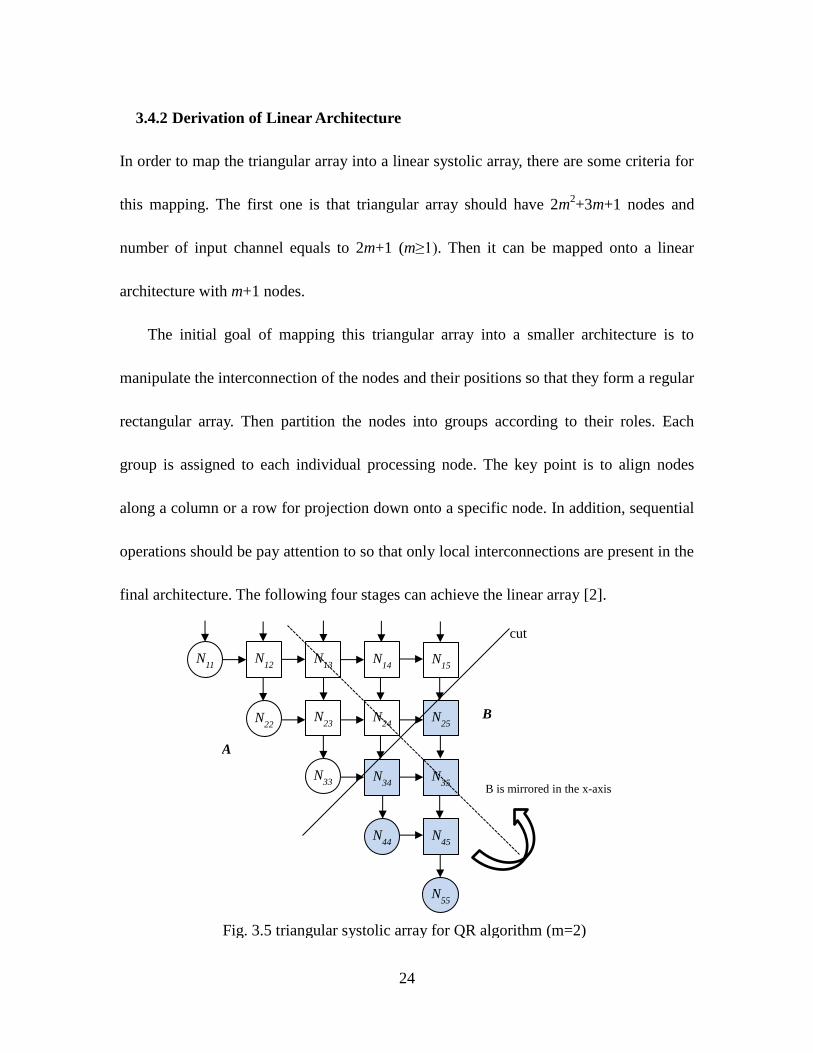
3.4.2 Derivation of Linear Architecture

In order to map the triangular array into a linear systolic array, there are some criteria for

this mapping. The first one is that triangular array should have 2m2+3m+1 nodes and

number of input channel equals to 2m+1 (m≥1). Then it can be mapped onto a linear

architecture with m+1 nodes.

The initial goal of mapping this triangular array into a smaller architecture is to

manipulate the interconnection of the nodes and their positions so that they form a regular

rectangular array. Then partition the nodes into groups according to their roles. Each

group is assigned to each individual processing node. The key point is to align nodes

along a column or a row for projection down onto a specific node. In addition, sequential

operations should be pay attention to so that only local interconnections are present in the

final architecture. The following four stages can achieve the linear array [2].

Fig. 3.5 triangular systolic array for QR algorithm (m=2)

N11 N

12 N

13 N

14 N

15

N22 N

23 N

24 N

25

N33 N

34 N

35

N44 N

45

N55

cut

A

B

B is mirrored in the x-axis

25

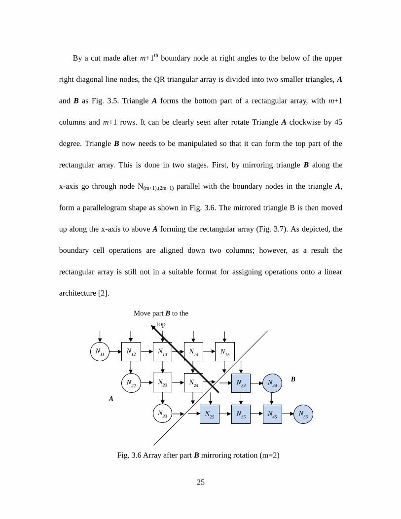
By a cut made after m+1th

boundary node at right angles to the below of the upper

right diagonal line nodes, the QR triangular array is divided into two smaller triangles, A

and B as Fig. 3.5. Triangle A forms the bottom part of a rectangular array, with m+1

columns and m+1 rows. It can be clearly seen after rotate Triangle A clockwise by 45

degree. Triangle B now needs to be manipulated so that it can form the top part of the

rectangular array. This is done in two stages. First, by mirroring triangle B along the

x-axis go through node N(m+1),(2m+1) parallel with the boundary nodes in the triangle A,

form a parallelogram shape as shown in Fig. 3.6. The mirrored triangle B is then moved

up along the x-axis to above A forming the rectangular array (Fig. 3.7). As depicted, the

boundary cell operations are aligned down two columns; however, as a result the

rectangular array is still not in a suitable format for assigning operations onto a linear

architecture [2].

Fig. 3.6 Array after part B mirroring rotation (m=2)

A

B

N25

N34

N35

N44

N45 N

55

N11 N

12 N

13 N

14 N

15

N22 N

23 N

24

N33

Move part B to the

top

26

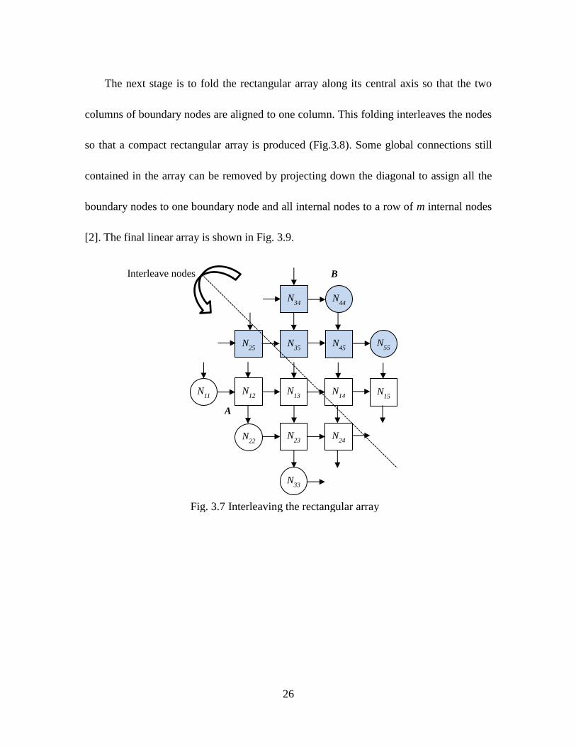
The next stage is to fold the rectangular array along its central axis so that the two

columns of boundary nodes are aligned to one column. This folding interleaves the nodes

so that a compact rectangular array is produced (Fig.3.8). Some global connections still

contained in the array can be removed by projecting down the diagonal to assign all the

boundary nodes to one boundary node and all internal nodes to a row of m internal nodes

[2]. The final linear array is shown in Fig. 3.9.

Fig. 3.7 Interleaving the rectangular array

A

B

N25

N34

N35

N44

N45 N

55

N11 N

12 N

13 N

14 N

15

N22 N

23 N

24

N33

Interleave nodes

27

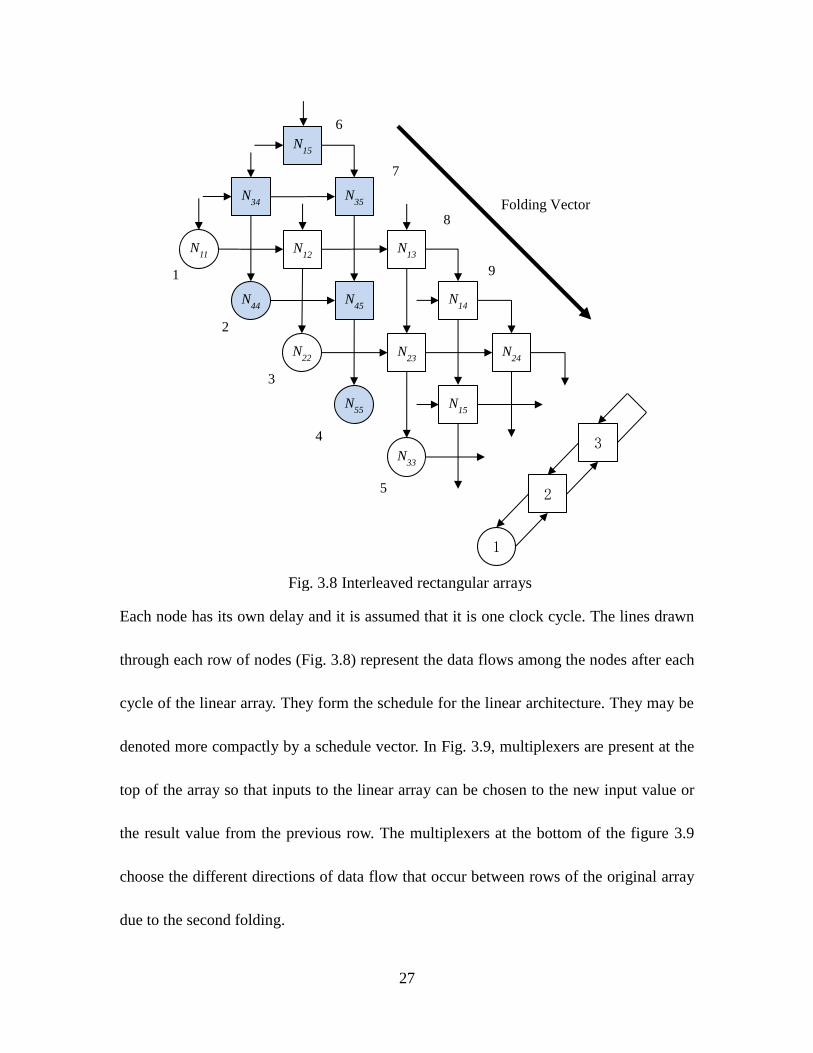
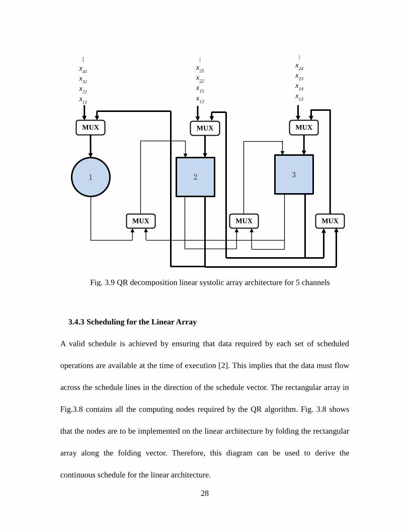
Each node has its own delay and it is assumed that it is one clock cycle. The lines drawn

through each row of nodes (Fig. 3.8) represent the data flows among the nodes after each

cycle of the linear array. They form the schedule for the linear architecture. They may be

denoted more compactly by a schedule vector. In Fig. 3.9, multiplexers are present at the

top of the array so that inputs to the linear array can be chosen to the new input value or

the result value from the previous row. The multiplexers at the bottom of the figure 3.9

choose the different directions of data flow that occur between rows of the original array

due to the second folding.

Fig. 3.8 Interleaved rectangular arrays

N15

N34 N

35

N44 N

45

N55

N11 N

12 N

13

N14

N15

N22 N

23 N

24

N33

Folding Vector

2

3

1

1

2

3

4

5

6

7

8

9

28

3.4.3 Scheduling for the Linear Array

A valid schedule is achieved by ensuring that data required by each set of scheduled

operations are available at the time of execution [2]. This implies that the data must flow

across the schedule lines in the direction of the schedule vector. The rectangular array in

Fig.3.8 contains all the computing nodes required by the QR algorithm. Fig. 3.8 shows

that the nodes are to be implemented on the linear architecture by folding the rectangular

array along the folding vector. Therefore, this diagram can be used to derive the

continuous schedule for the linear architecture.

2 3 1

MUX

MUX

MUX

MUX

MUX

MUX

⁞

x25

x22

x15

x12

⁞

x24

x23

x14

x13

⁞

x41

x31

x21

x11

Fig. 3.9 QR decomposition linear systolic array architecture for 5 channels

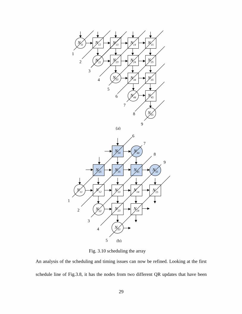
29

An analysis of the scheduling and timing issues can now be refined. Looking at the first

schedule line of Fig.3.8, it has the nodes from two different QR updates that have been

Fig. 3.10 scheduling the array

N11 N

12 N

13 N

14 N

15

N22 N

23 N

24 N

25

N33 N

34 N

35

N44 N

45

N55

1

2

3

4

5

6

7

8

9 (a)

(b)

N25

N34

N35

N44

N45 N

55

N11 N

12 N

13 N

14 N

15

N22 N

23 N

24

N33

1

2

3

4

5

6

7

8

9

30

interleaved. One QR update means that all the stored values r inside each node have been

updated once or all nodes have been executed once. This can be more easily visualized by

considering the schedule of the unfolded array shown in Fig.3.10 (a). Figure 3.10(b)

shows the array and the schedule after array rotation and moving. The colored QR nodes

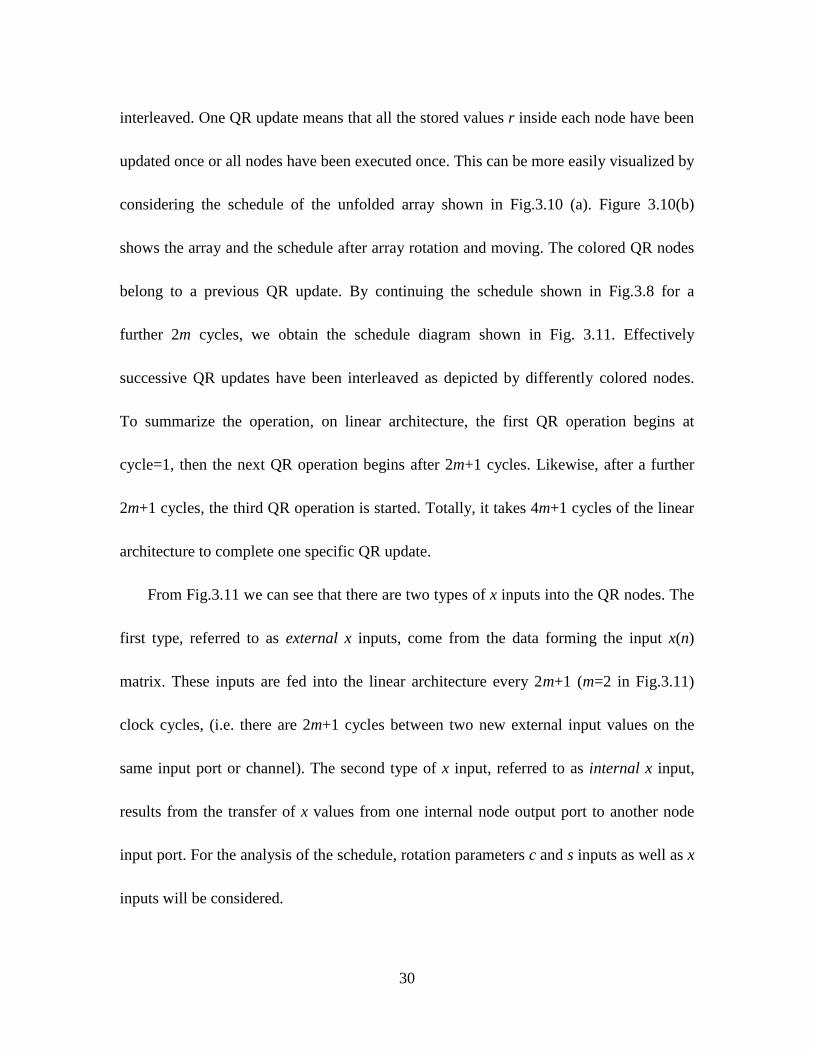
belong to a previous QR update. By continuing the schedule shown in Fig.3.8 for a

further 2m cycles, we obtain the schedule diagram shown in Fig. 3.11. Effectively

successive QR updates have been interleaved as depicted by differently colored nodes.

To summarize the operation, on linear architecture, the first QR operation begins at

cycle=1, then the next QR operation begins after 2m+1 cycles. Likewise, after a further

2m+1 cycles, the third QR operation is started. Totally, it takes 4m+1 cycles of the linear

architecture to complete one specific QR update.

From Fig.3.11 we can see that there are two types of x inputs into the QR nodes. The

first type, referred to as external x inputs, come from the data forming the input x(n)

matrix. These inputs are fed into the linear architecture every 2m+1 (m=2 in Fig.3.11)

clock cycles, (i.e. there are 2m+1 cycles between two new external input values on the

same input port or channel). The second type of x input, referred to as internal x input,

results from the transfer of x values from one internal node output port to another node

input port. For the analysis of the schedule, rotation parameters c and s inputs as well as x

inputs will be considered.

31

Fig. 3.11 Interleaved QR iteration (m=2)

1

10

N25 N

34 N

11

N35 N

12 N

44

N13 N

45 N

22

N14 N

23 N

55

N24 N

15 N

33

N25 N

34 N

11

N35 N

12 N

44

N13 N

45 N

22

N14 N

23 N

55

N24 N

15 N

33

N25 N

34 N

11

N35 N

12 N

44

N13 N

45 N

22

N14 N

23 N

55

N24 N

15 N

33

N25 N

34 N

11

N35 N

12 N

44

N13 N

45 N

22

N14 N

23 N

55

N24 N

15 N

33

N25 N

34 N

11

N35 N

12 N

44

N13 N

45 N

22

N14 N

23 N

55

N24 N

15 N

33

N25 N

34 N

11

N35 N

12 N

44

N13 N

45 N

22

N14 N

23 N

55

N24 N

15 N

33

11

20

29

21

White node means idle

Color node means executing

x1(1)

x2(1)

x3(1)

x4(1)

x5(1)

x1(2)

x2(2)

x3(2)

x4(2)

x5(2)

x1(3)

x2(3)

x3(3)

x4(3)

x5(3)

x1(4)

x2(4)

x3(4)

x4(4)

x5(4)

x1(5)

x2(5)

x3(5)

x4(5)

x5(5)

32

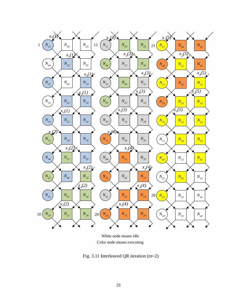
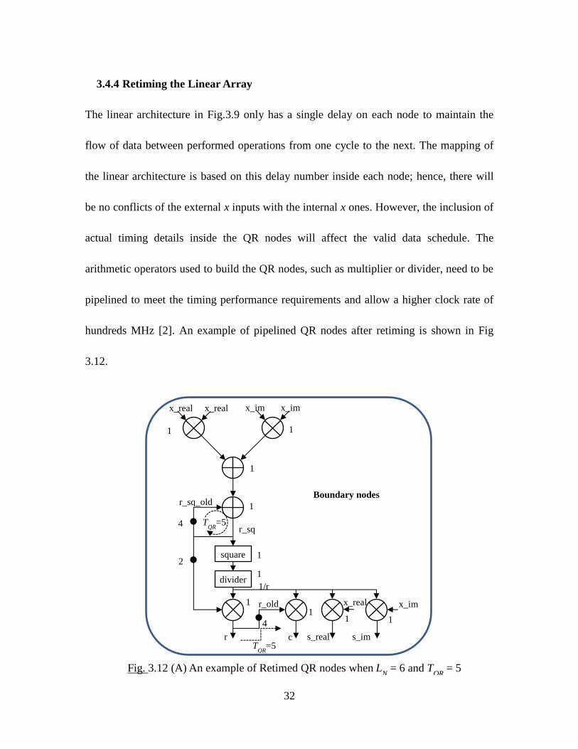
3.4.4 Retiming the Linear Array

The linear architecture in Fig.3.9 only has a single delay on each node to maintain the

flow of data between performed operations from one cycle to the next. The mapping of

the linear architecture is based on this delay number inside each node; hence, there will

be no conflicts of the external x inputs with the internal x ones. However, the inclusion of

actual timing details inside the QR nodes will affect the valid data schedule. The

arithmetic operators used to build the QR nodes, such as multiplier or divider, need to be

pipelined to meet the timing performance requirements and allow a higher clock rate of

hundreds MHz [2]. An example of pipelined QR nodes after retiming is shown in Fig

3.12.

Boundary nodes

x_im

square

divider


r_sq_old

r_sq

r

r_old

1/r

x_real

c s_real s_im

1 1

1

1

1

1

1 1 1

4

2

1

4

TQR

=5

TQR

=5

Fig. 3.12 (A) An example of Retimed QR nodes when LN = 6 and T

QR = 5

33

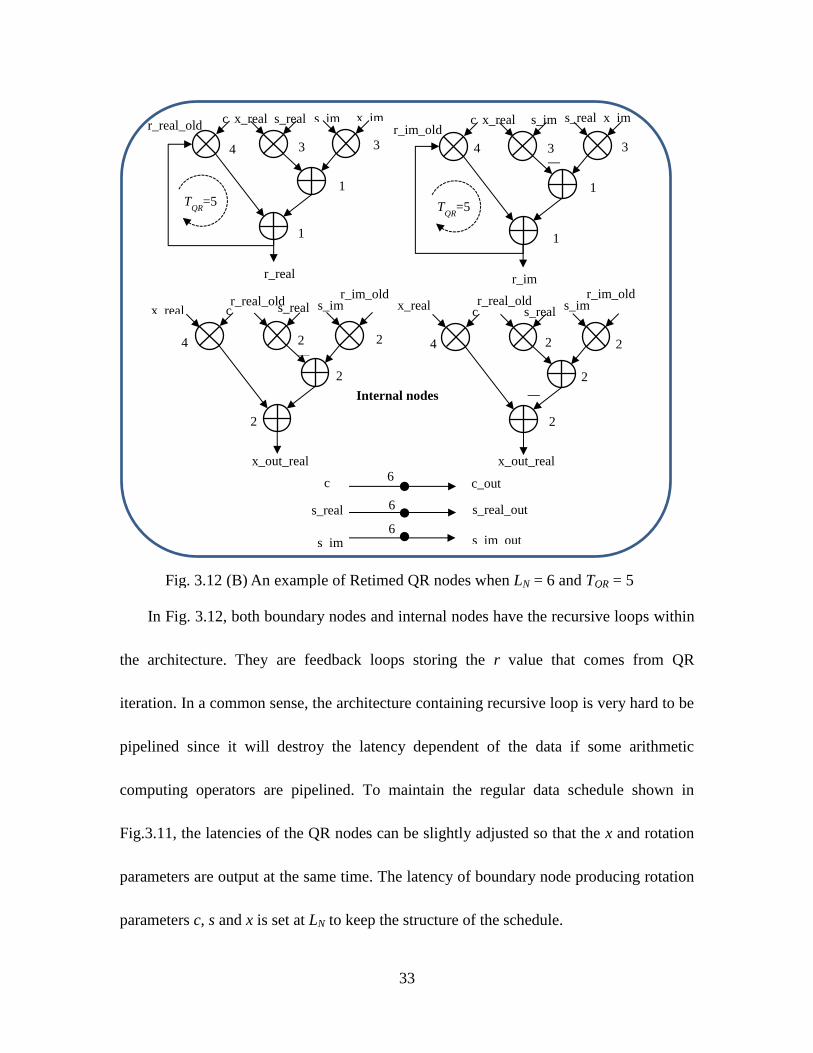
In Fig. 3.12, both boundary nodes and internal nodes have the recursive loops within

the architecture. They are feedback loops storing the r value that comes from QR

iteration. In a common sense, the architecture containing recursive loop is very hard to be

pipelined since it will destroy the latency dependent of the data if some arithmetic

computing operators are pipelined. To maintain the regular data schedule shown in

Fig.3.11, the latencies of the QR nodes can be slightly adjusted so that the x and rotation

parameters are output at the same time. The latency of boundary node producing rotation

parameters c, s and x is set at LN to keep the structure of the schedule.

Fig. 3.12 (B) An example of Retimed QR nodes when LN = 6 and TQR = 5

c r_real_old

s_real s_imr_im_old

x_out_real

x_real

4

2

2 2

2


r_real

r_real_old

3 3

1

4

1

TQR

=5


r_im

r_im_old

4 3 3

1

1

TQR

=5

c r_real_old

s_real s_im

r_im_old

x_out_real

x_real

4 2 2

2

2

Internal nodes

c

s_real

s_im

c_out

s_real_out

s_im_out

6

6

6

—

—

—

34

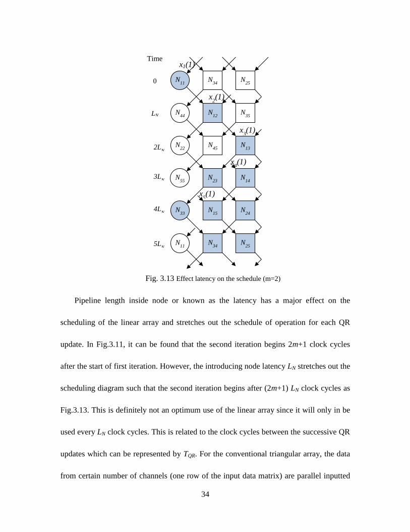
Pipeline length inside node or known as the latency has a major effect on the

scheduling of the linear array and stretches out the schedule of operation for each QR

update. In Fig.3.11, it can be found that the second iteration begins 2m+1 clock cycles

after the start of first iteration. However, the introducing node latency LN stretches out the

scheduling diagram such that the second iteration begins after (2m+1) LN clock cycles as

Fig.3.13. This is definitely not an optimum use of the linear array since it will only in be

used every LN clock cycles. This is related to the clock cycles between the successive QR

updates which can be represented by TQR. For the conventional triangular array, the data

from certain number of channels (one row of the input data matrix) are parallel inputted

Fig. 3.13 Effect latency on the schedule (m=2)

0 N25 N

34 N

11

N35 N

12 N

44

N13 N

45 N

22

N14 N

23 N

55

N24 N

15 N

33

N25 N

34 N

11

x1(1)

x2(1)

x3(1)

x4(1)

x5(1)

LN

2LN

3LN

4LN

5LN

Time

35

to the array on every clock cycle. The recursive loops have to be updated every clock

cycle. However, for the QR-D linear array, the data of each channel on one QR update

have to be inputted serially. This means, for each node, that the recursive loops do not

have to be updated every clock cycle but updated every TQR clock cycle. This can help to

pipeline the recursive loop to TQR length. Therefore, a high data sampling rate should be

achieved. The goal is to find the proper combination of LN and TQR that can guarantee a

valid schedule and 100 percent hardware utilization.

From G. Lightbody’s work [2], the value for TQR is the same as the number of input

channels of the original QR triangular array, which is 2m+1. This can be seen that it

equates to the level of hardware reduction that was obtained from mapping of 2m2+3m+1

nodes triangular array down to m+1 nodes linear array. Also, by setting the node latency

LN to a relatively prime number of TQR, a valid schedule can be achieved. If these two

numbers are not relatively prime number, then there will be data collision at the products

of LN and TQR with their common multiplies.

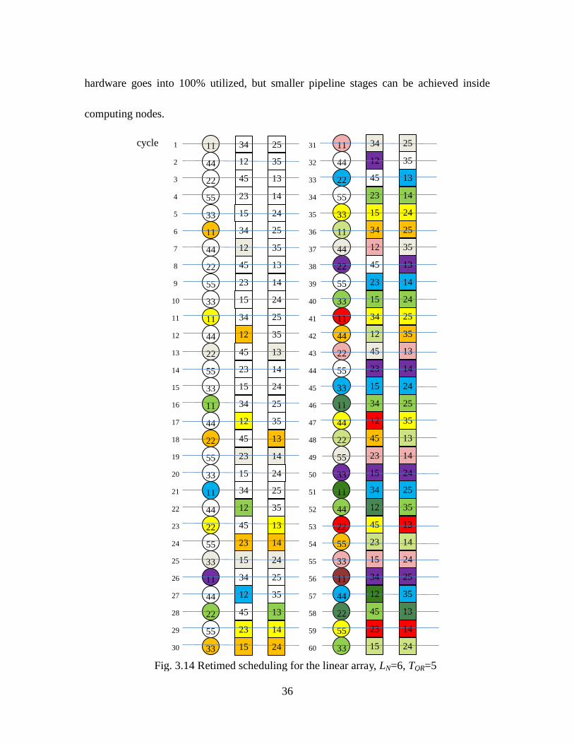
Furthermore, choosing an optimum value of LN and TQR is to ensure that the nodes

are fully utilized. Fig 3.14 shows the example schedule over several QR updates when LN

is 6 and TQR is 5. The different colored nodes represent different QR iterations that are

interleaved with each other to fill the blank nodes left by the highlighted QR iteration.

When there is no blank node, the array is under 100 percent hardware utilized. We can

find this array is on 100 percent utilization after 45 cycles. The smaller LN, the faster

36

hardware goes into 100% utilized, but smaller pipeline stages can be achieved inside

computing nodes.

Fig. 3.14 Retimed scheduling for the linear array, LN=6, TQR=5

1

2

3

4

5

6

7

8

9

10

11

12

13

14

15

16

17

18

19

20

21

22

23

24

25

26

27

28

29

30

31

32

33

34

35

36

37

38

39

40

41

42

43

44

45

46

47

48

49

50

51

52

53

54

55

56

57

58

59

60

11

13 45 22

14 23 55

24 15 33

25 34 11

35 12 44

13 45 22

14 23 55

24 15 33

25 34 11

35 12 44

13 45 22

14 23 55

24 15 33

25 34 11

35 12 44

13 45 22

14 23 55

24 15 33

25 34 11

35 12 44

13 45 22

14 23 55

24 15 33

25 34 11

35 12 44

13 45 22

14 23 55

24 15 33

25 34 11

35 12 44

13 45 22

14 23 55

24 15 33

25 34 11

35 12 44

13 45 22

14 23 55

24 15 33

25 34 11

35 12 44

13 45 22

14 23 55

24 15 33

25 34 11

35 12 44

13 45 22

14 23 55

24 15 33

25 34 11

35 12 44

13 45 22

14 23 55

24 15 33

25 34 11

35 12 44

13 45 22

14 23 55

24 15 33

cycle 25 34

35 12 44

37

4. QR DECOMPOSITION IMPLEMENTATION

Introduction of FPGA Design 4.1

In recent years, rapid advancement of Field Programmable Gate Array (FPGA)

technology is enabling highly reliable re-programmable solutions. By implementing over

the logical level not the physical circuits, users can better focus on the algorithm and

architecture optimization. It helps to accelerate the system design.

In this thesis, The QR decomposition based on Givens rotations algorithm is

implemented on both conventional QR systolic triangular array and linear QR array on

Xilinx Virtex 6 FPGA. The input and output data as well as arithmetic operation of QR

processors are in fix-point format. Fix-point square root inverse is implemented by

polynomial approximation. Compared with CORDIC or square-root-free algorithm, this

implementation is better understood and easier to establish. Challenges include how to

pipeline each computation node and how to implement linear systolic by folding

triangular array. The retiming and rescheduling on linear systolic also require deep

understanding of latency dependence between each node.

4.1.1 FPGA Introduction

Field Programmable Gate Array short for FPGA belongs to the programmable logical

devices family. It is generated from the rapid evolution of very large scale circuit (VLSI)

and computer aided design (CAD) technology. FPGA has properties of high integration,

38

high speed of processing, reprogrammability, and low cost. Circuit designers can do the

logical programming, compiling, optimization, simulation and verification based on the

limited funding and short development period. This is an efficient method for VLSI

prototyping. FPGA chips also integrate massive physical IP (Intelligent patent) cores to

decrease power consummation and increase reliability. It also helps to increase

processing speed.

The basic logical unit of FPGA is a look-up table. By loading the pre-defined logical

bits stream stored in external memory generated from CAD software, FPGA can easily

establish the corresponding logical relation inside the chip. Power off the chip, the logical

relation will is wiped. In this way, FPGA can be reusable or reprogrammable.

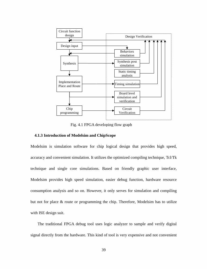
4.1.2 FPGA Design Process

The design of FPGA is based on the idea of top – down. It contains circuit functions

design, design input, function simulation, synthesis optimization, synthesis post

simulation, implementation design, post simulation of place & route, board level

simulation and chip programming and debug. Fig 4.1 shows a general design flow graph.

39

4.1.3 Introduction of Modelsim and ChipScope

Modelsim is simulation software for chip logical design that provides high speed,

accuracy and convenient simulation. It utilizes the optimized compiling technique, Tcl/Tk

technique and single core simulations. Based on friendly graphic user interface,

Modelsim provides high speed simulation, easier debug function, hardware resource

consumption analysis and so on. However, it only serves for simulation and compiling

but not for place & route or programming the chip. Therefore, Modelsim has to utilize

with ISE design suit.

The traditional FPGA debug tool uses logic analyzer to sample and verify digital

signal directly from the hardware. This kind of tool is very expensive and not convenient

Fig. 4.1 FPGA developing flow graph

Circuit function

design

Design input

Synthesis

Implementation

Place and Route

Chip

programming Circuit

Verification

Board level

simulation and

verification

Timing simulation

Static timing

analysis

Synthesis post

simulation

Behaviors

simulation

Design Verification

40

for testing since too many chip probes need to be connected. Therefore, Xilinx provides

ChipScope Pro logical analyzing tool. This software based tool inserts a particular IP core,

connecting to the net or port that needs analyzing, into the FPGA design. Users can

analysis the signal sampled by the analyzer IP core via JTAG (Joint Test Action Group)

port under ChipScope Pro analyzer GUI (graphic user interface). In this method, under

the system’s required clock frequency, users can directly analysis the signals inside FPGA

chip without any interference on the circuit function. This software based analyzer can

implement high level trigger functions to filter out and display any design problems

without re-synthesis but simply by changing the soft probe.

Utilizing the advanced functions of Modelsim and ChipScope Pro, the QRD design

described in this thesis is developed under Xilinx ISE FPGA design suit, simulated on

Modelsim and verified under ChipScope Pro.

Implementation by the Triangular Array 4.2

In J. G. McWhirter’s published paper, the triangular array is well defined. In Chapter 3,

the details of triangular array for QR decomposition are discussed specifically. However,

there are still several problems left unsolved. First, we can see each computing node only

has one latency or one delay. This means the result value will show up one clock cycles

later than the input value. Thu, this one clock cycle should long enough to meet the least

time consisting of the max length of the combination logical circuit inside each node. In

41

this case, the main clock frequency has to maintain at low speed and the data throughput

rate will be hurt. In order to avoid this situation, in the following design, pipeline will be

applied into each computing nodes, and the whole macro architecture will be slightly

modified.

The second issue involves the square root inverse. To compute the rotation

parameters, the square root inverse is inevitable. However, square root inverse is a very

complicated operation for VLSI implementation when the speed and accuracy are

concerned. So far, there are three ways to solve the square root inverse for QR

decomposition, which are CORDIC algorithm, Logarithm and root square free QRD.

Considering convenience, speed and latency, a Logarithm method combining look-up

table will be used for implementing square root inverse in this thesis.

4.2.1 Boundary Node

Usually, for the real system, the data input into the QR decomposition array usually do

not directly come from ADC (analog to digital converter). There are certain devices

between them like digital filter. Thus, a signed 16 bits fixed-point integer was chosen as

the input data format since 14 bits ADC is commonly used in radio system and 2 bits is

reserved for redundant. Also a fixed number containing signed 19 bits integer with 3 bits

decimal was used as the r output data format. Signed 32 bits fix point decimal number

was applied for s_real and s_im output. Unsigned 32 bits fix point decimal number was

used for c value output.

42

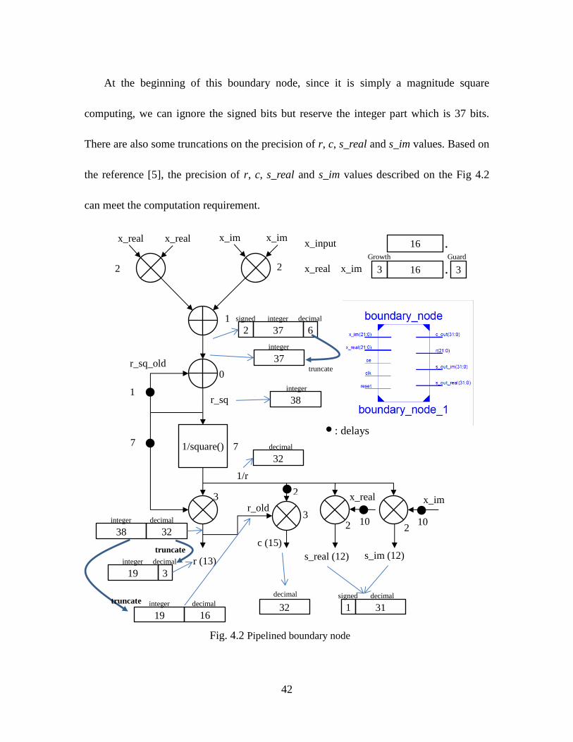
At the beginning of this boundary node, since it is simply a magnitude square

computing, we can ignore the signed bits but reserve the integer part which is 37 bits.

There are also some truncations on the precision of r, c, s_real and s_im values. Based on

the reference [5], the precision of r, c, s_real and s_im values described on the Fig 4.2

can meet the computation requirement.

Fig. 4.2 Pipelined boundary node

x_im

1/square()


r_sq_old

r_sq

r (13)

r_old

1/r

x_real

c (15)

s_real (12) s_im (12)

2 2

1

7

3 2 2

1

7

3 2

10 10

16

16 3 3

.

. x_real x_im

x_input

Growth Guard

37 2 signed integer

6 decimal

37 integer

truncate

38 integer

32 decimal

19 integer

3 decimal

38 integer

32 decimal

19 integer

16 decimal

32

decimal

31 1 signed decimal

: delays

truncate

truncate

0

43

There is also a difference of the boundary node in Fig. 4.2 comparing with the

conventional boundary node. The conventional triangular QRD array requires that each

node has the same latency on the output rotation parameters c and s. However, in Fig. 4.2,

the pipeline length on c value is 15 clock cycles but the pipeline length on s value is 12

clock cycles. This is not a fault but a compromise on the reclusive loop inside the internal

node. This will be discussed in following section. We can simply regard the boundary

computing latency or pipeline length is 12 clock cycles for rotation parameters computing

except for r because r value will not involve in the computation of the internal node. It is

simply the result value on the diagonal of the upper triangular matrix. In a word, this

method will pipeline the boundary node to 12 stages. This helps to increase the input data

sampling frequency.

4.2.2 Square Root Inverse

As we know, square root inverse is a complicated operation for VLSI implementation.

But it is still feasible. In this thesis, a polynomial approximation will help to solve square

root inverse.

For common square root inverse, the input value range is over (0, +∞] and the output

value range is also over (0, +∞]. In our boundary node configuration, the input of square

root inverse is over [1, 238

]. Thus, the output is over [2-19

, 1]. Even though it seems the

input and output range is fixed and smaller than the normal square root inverse. However,

it is still a problem to do this operation, because there is no any basic operator for VLSI

44

circuit. It must be done by a combination of many basic operators, for example multiplier,

divider, and adder. However, the latency and speed will be a big problem. CORDIC

algorithm is better choice since it can really provide a high precise result but the latency

or called delay is too much. The same operation done by CORDIC ip core and divider ip

core from Xilinx will take almost 20 clock cycles. It provides more accuracy, but

sacrifices on the latency and speed. We need an alternative way with low latency but high

clock frequency.

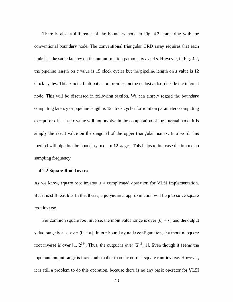
Polynomial approximation is better method to balance the latency and precision. For

any input value, it can be mapped to [1, 2) simply by shifting certain positions. For a

particular value r_sq (r_sq≥1, which is an unsigned number) represented by binary form,

it definitely always has the most significant bit which is 1. For example r_sq = (9999)10 =

(10011100001111)2, we can always shift the decimal point to the right of the most

significant bit. Then we get r_sq_normalized = (1.0011100001111)2. This normalized

value is always on the range of [1, 2). Thus, the problem is simplified to do square root

inverse over range of [1, 2).

45

Fig. 4.3 Polynomial Approximation to 1/sqrt() [5]

1 1.2 1.4 1.6 1.8 20.7

0.75

0.8

0.85

0.9

0.95

1

y=Ax+B

A B

Ax+B=y

X=1x37x36x35……x3x2x1

Xnormalized=1. x37x36x35…….x3x2x1

addressing

realign output

MEM

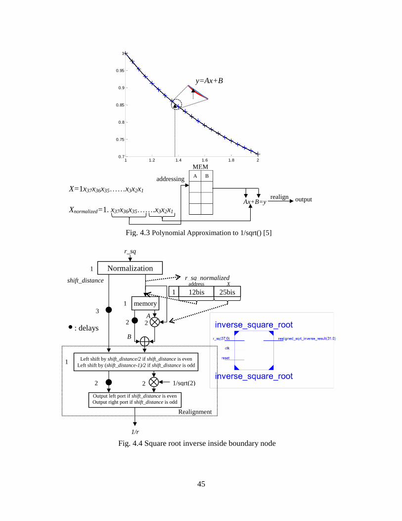
Fig. 4.4 Square root inverse inside boundary node

r_sq

Normalization 1

3 memory

r_sq_normalized shift_distance

12bis 1 address

25bis X

A

B

1

2

Realignment

Left shift by shift_distance/2 if shift_distance is even

Left shift by (shift_distance-1)/2 if shift_distance is odd

1

1/sqrt(2)

Output left port if shift_distance is even

Output right port if shift_distance is odd

1/r

2

: delays

2

2

46

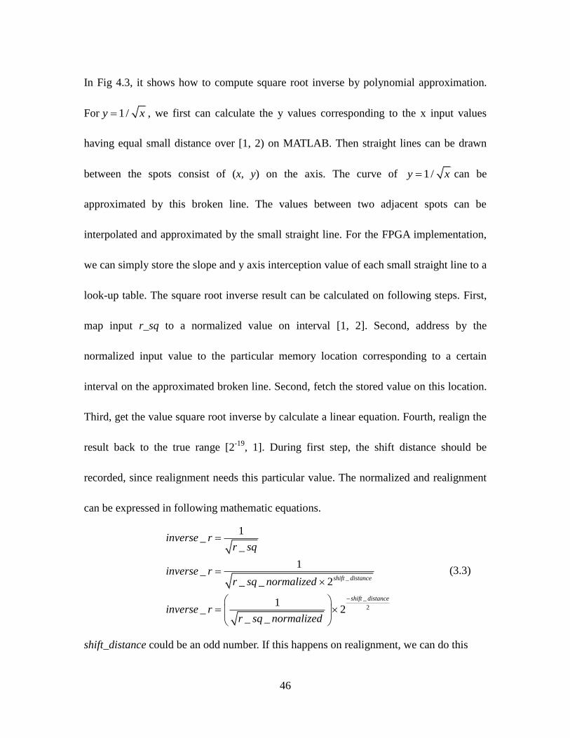
In Fig 4.3, it shows how to compute square root inverse by polynomial approximation.

For 1/y x , we first can calculate the y values corresponding to the x input values

having equal small distance over [1, 2) on MATLAB. Then straight lines can be drawn

between the spots consist of (x, y) on the axis. The curve of 1/y x can be

approximated by this broken line. The values between two adjacent spots can be

interpolated and approximated by the small straight line. For the FPGA implementation,

we can simply store the slope and y axis interception value of each small straight line to a

look-up table. The square root inverse result can be calculated on following steps. First,

map input r_sq to a normalized value on interval [1, 2]. Second, address by the

normalized input value to the particular memory location corresponding to a certain

interval on the approximated broken line. Second, fetch the stored value on this location.

Third, get the value square root inverse by calculate a linear equation. Fourth, realign the

result back to the true range [2-19

, 1]. During first step, the shift distance should be

recorded, since realignment needs this particular value. The normalized and realignment

can be expressed in following mathematic equations.

_

_

2

1_

_

1_

_ _ 2

1_ 2

_ _

shift distance

shift distance

inverse rr sq

inverse rr sq normalized


(3.3)

shift_distance could be an odd number. If this happens on realignment, we can do this

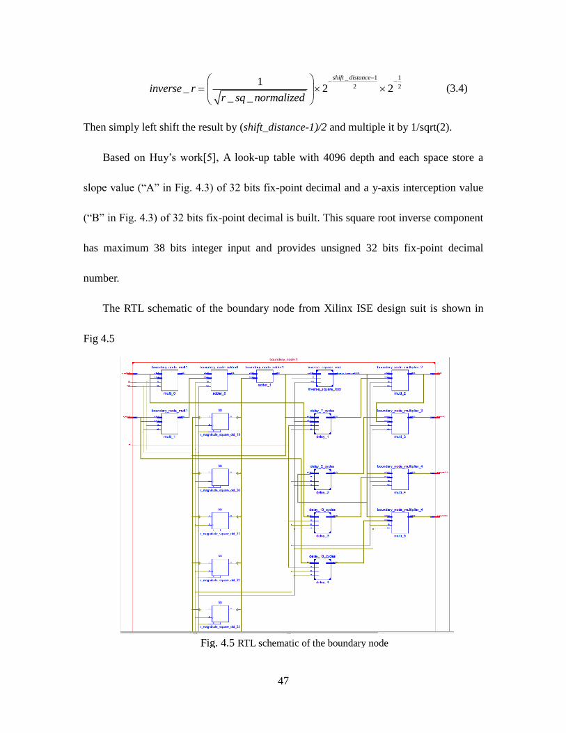
47

_ 1 1

2 21

_ 2 2_ _

shift distance


(3.4)

Then simply left shift the result by (shift_distance-1)/2 and multiple it by 1/sqrt(2).

Based on Huy’s work[5], A look-up table with 4096 depth and each space store a

slope value (“A” in Fig. 4.3) of 32 bits fix-point decimal and a y-axis interception value

(“B” in Fig. 4.3) of 32 bits fix-point decimal is built. This square root inverse component

has maximum 38 bits integer input and provides unsigned 32 bits fix-point decimal

number.

The RTL schematic of the boundary node from Xilinx ISE design suit is shown in

Fig 4.5

Fig. 4.5 RTL schematic of the boundary node

48

4.2.3 Internal Node

The internal node is shown in Fig 4.6. All operators such as multiplier, adder and

subtractor are implemented by Xilinx IP core. The multipliers are implemented by on

chip DSP cell which can help to increase frequency and decrease latency. Adders and

subtractors are formed by logical slices.

However, there are two recursive loops containing multiplier and adder on the path

for calculating r_real and r_im. They will affect the internal clock frequency since the

recursive loop is not easily to be pipelined under the triangular systolic array

configuration. Not only does the recursive loop decrease clock frequency, but it also

badly affects their parallel paths, as in the left branches on calculating r_real and r_im. If

all the inputs, for example c, s_real, s_im, x_real, x_im, arrive at same time, the recursive

loop Path 1(Fig 4.6) must be finished in one clock cycle, Path 2 also must be done in one

clock cycle. However, Path 2 is much longer than Path 1. This is not an efficient method

to finish Path 2 in one clock cycle. To avoid this happening, make the c arrives 3 clock

cycles later than s_real and s_im. In this way, the Path 2 can be pipelined by 3 levels and

will not be affected by the recursive loop too much. Pipeline of the recursive loop can

only be done under linear systolic array. This is discussed in Chapter 3.

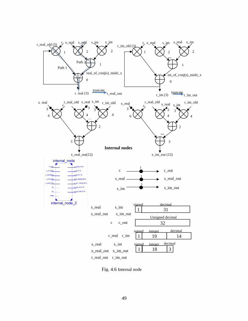
49

Fig. 4.6 Internal node

c r_real_old s_real s_im

r_im_old

x_real_out(12)

x_real

6

3

4 4

2


r_real (3)

r_real_old (3)

2 2

1

1

0


r_im (3)

r_im_old (3) 1 2 2

1

0

c r_real_old

s_real s_imr_im_old

x_im_out (12)

x_real

6 4 4

2

3

Internal nodes

3 3 3 3

—

—

—

real_of_conj(s)_multi_x im_of_conj(s)_multi_x

Path 1 Path 2

c

s_real

s_im

c_out

s_real_out

s_im_out

1

1

1

3 3

31 1 signed decimal

s_real s_im

s_real_out s_im_out

32 Unsigned decimal

c c_out

19 1 signed integer

14 decimal

r_real r_im

18 1 signed integer

3

decimal x_real x_im

x_real_out x_im_out

r_real_out r_im_out

r_real_out r_im_out truncate

truncate

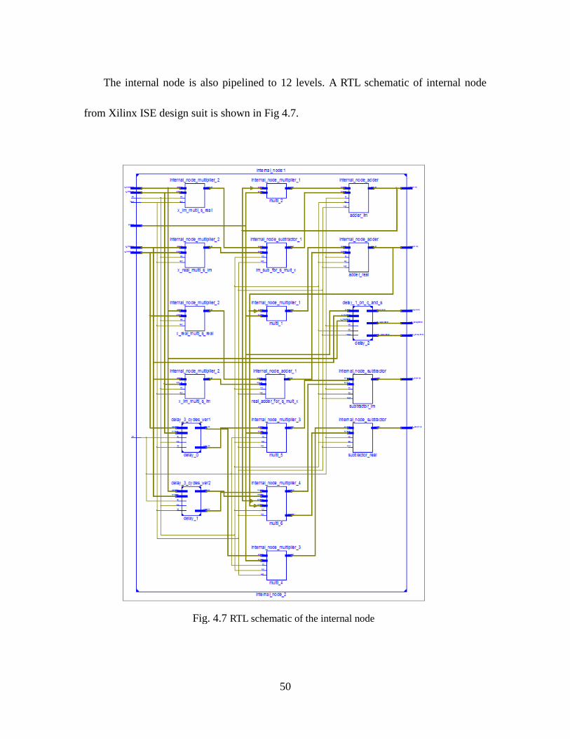
50

The internal node is also pipelined to 12 levels. A RTL schematic of internal node

from Xilinx ISE design suit is shown in Fig 4.7.

Fig. 4.7 RTL schematic of the internal node

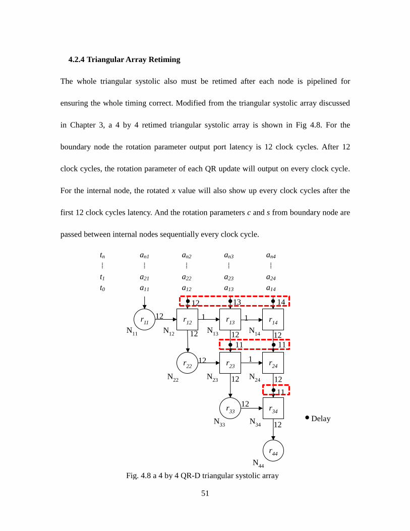
51

4.2.4 Triangular Array Retiming

The whole triangular systolic also must be retimed after each node is pipelined for

ensuring the whole timing correct. Modified from the triangular systolic array discussed

in Chapter 3, a 4 by 4 retimed triangular systolic array is shown in Fig 4.8. For the

boundary node the rotation parameter output port latency is 12 clock cycles. After 12

clock cycles, the rotation parameter of each QR update will output on every clock cycle.

For the internal node, the rotated x value will also show up every clock cycles after the

first 12 clock cycles latency. And the rotation parameters c and s from boundary node are

passed between internal nodes sequentially every clock cycle.

Fig. 4.8 a 4 by 4 QR-D triangular systolic array

tn an1 an2 an3 an4

⁞ ⁞ ⁞ ⁞ ⁞

t1 a21 a22 a23 a24

t0 a11 a12 a13 a14

r11 r

12 r

13 r

14

r22 r

23 r

24

r33 r

34

r44

N11 N

12 N

13 N

14

N22 N

23 N

24

N33 N

34

N44

12 13 14

1 1

11 11

1

11

12

12

12

12

12 12

12

12

12 Delay

s

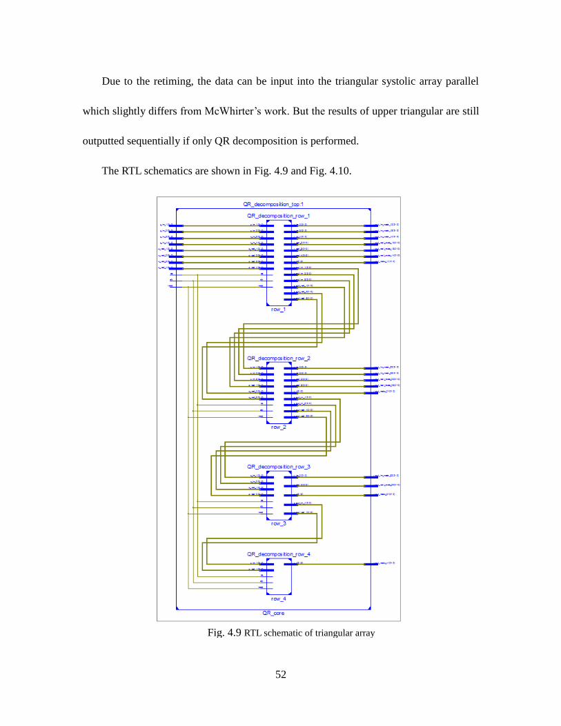
52

Due to the retiming, the data can be input into the triangular systolic array parallel

which slightly differs from McWhirter’s work. But the results of upper triangular are still

outputted sequentially if only QR decomposition is performed.

The RTL schematics are shown in Fig. 4.9 and Fig. 4.10.

Fig. 4.9 RTL schematic of triangular array

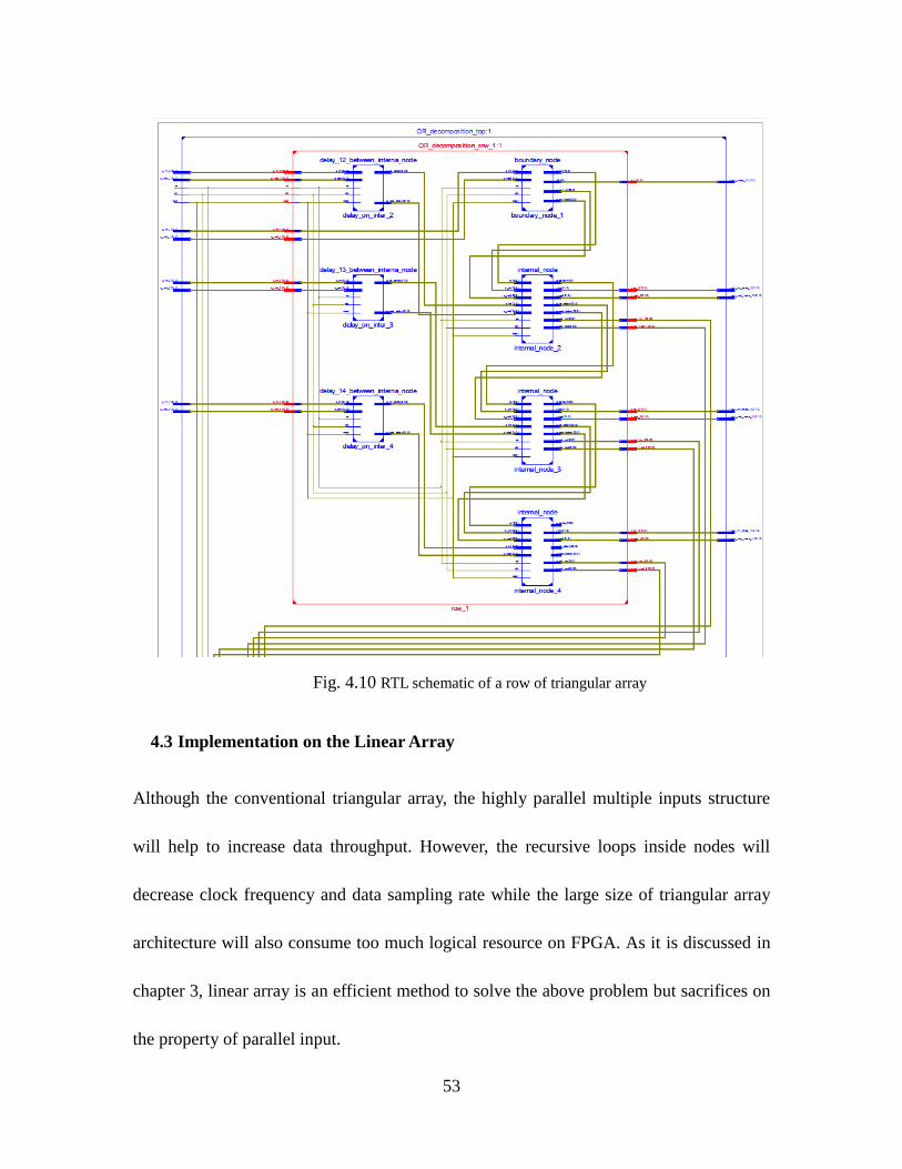
53

Implementation on the Linear Array 4.3

Although the conventional triangular array, the highly parallel multiple inputs structure

will help to increase data throughput. However, the recursive loops inside nodes will

decrease clock frequency and data sampling rate while the large size of triangular array

architecture will also consume too much logical resource on FPGA. As it is discussed in

chapter 3, linear array is an efficient method to solve the above problem but sacrifices on

the property of parallel input.

Fig. 4.10 RTL schematic of a row of triangular array

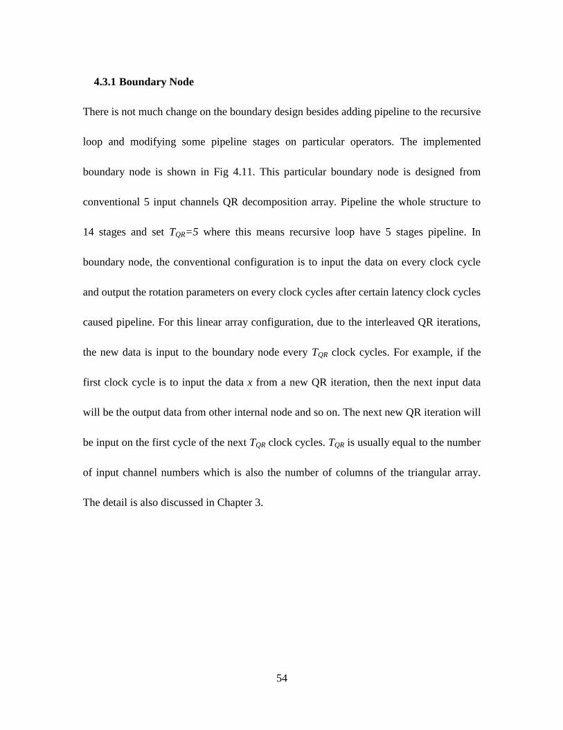
54

4.3.1 Boundary Node

There is not much change on the boundary design besides adding pipeline to the recursive

loop and modifying some pipeline stages on particular operators. The implemented

boundary node is shown in Fig 4.11. This particular boundary node is designed from

conventional 5 input channels QR decomposition array. Pipeline the whole structure to

14 stages and set TQR=5 where this means recursive loop have 5 stages pipeline. In

boundary node, the conventional configuration is to input the data on every clock cycle

and output the rotation parameters on every clock cycles after certain latency clock cycles

caused pipeline. For this linear array configuration, due to the interleaved QR iterations,

the new data is input to the boundary node every TQR clock cycles. For example, if the

first clock cycle is to input the data x from a new QR iteration, then the next input data

will be the output data from other internal node and so on. The next new QR iteration will

be input on the first cycle of the next TQR clock cycles. TQR is usually equal to the number

of input channel numbers which is also the number of columns of the triangular array.

The detail is also discussed in Chapter 3.

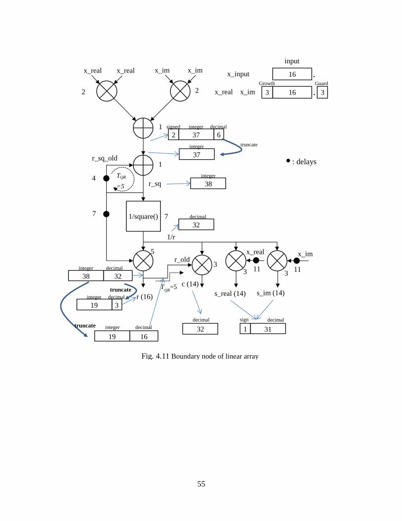
55

x_im

1/square()


r_sq_old

r_sq

r (16)

r_old

1/r

x_real

c (14) s_real (14) s_im (14)

2 2

1

7

3 3 3

4

7

5

11 11

16

16 3 3

.

. x_real x_im

x_input

input

Growth Guard

37 2 signed integer

6 decimal

37 integer truncate

38 integer

32 decimal

19 integer

3 decimal

38 integer

32 decimal

19

integer

16

decimal

32

decimal

31 1

sign decimal

: delays

Fig. 4.11 Boundary node of linear array

1

TQR

=5

TQR

=5 truncate

truncate

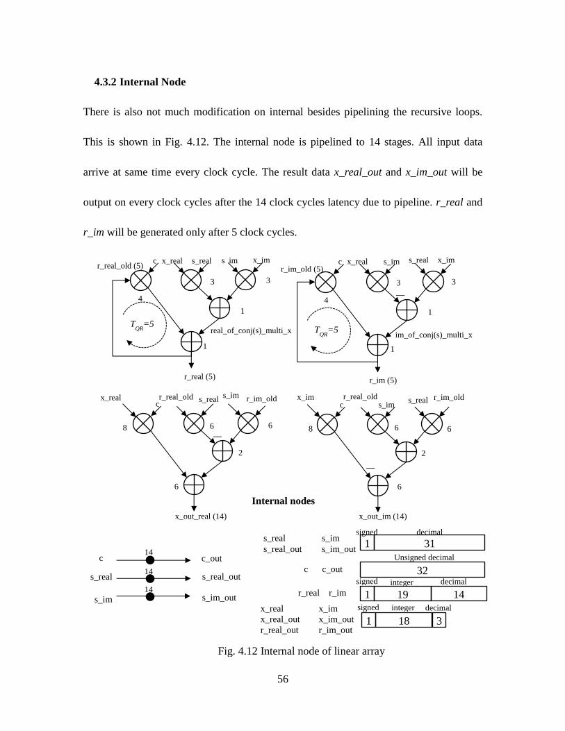
56

4.3.2 Internal Node

There is also not much modification on internal besides pipelining the recursive loops.

This is shown in Fig. 4.12. The internal node is pipelined to 14 stages. All input data

arrive at same time every clock cycle. The result data x_real_out and x_im_out will be

output on every clock cycles after the 14 clock cycles latency due to pipeline. r_real and

r_im will be generated only after 5 clock cycles.

c

s_real

s_im

c_out

s_real_out

s_im_out

14

14

14

Fig. 4.12 Internal node of linear array

c r_real_old s_real s_im r_im_old

x_out_real (14)

x_real

8

6

6 6

2


r_real (5)

r_real_old (5)

3 3

1 4

1


r_im (5)

r_im_old (5)

4

3 3

1

1

c r_real_old

s_im s_real r_im_old

x_out_im (14)

x_im

8 6 6

2

6

Internal nodes

—

—

real_of_conj(s)_multi_x im_of_conj(s)_multi_x

TQR

=5 T

QR=5

31 1 signed decimal

s_real s_im s_real_out s_im_out

32

Unsigned decimal c c_out

19 1

signed integer 14

decimal r_real r_im

18 1

signed integer

3

decimal x_real x_im x_real_out x_im_out r_real_out r_im_out

—

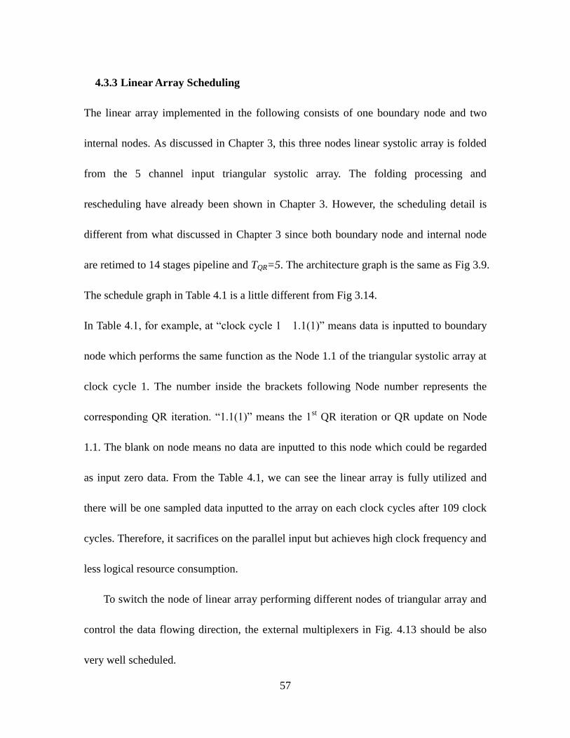
57

4.3.3 Linear Array Scheduling

The linear array implemented in the following consists of one boundary node and two

internal nodes. As discussed in Chapter 3, this three nodes linear systolic array is folded

from the 5 channel input triangular systolic array. The folding processing and

rescheduling have already been shown in Chapter 3. However, the scheduling detail is

different from what discussed in Chapter 3 since both boundary node and internal node

are retimed to 14 stages pipeline and TQR=5. The architecture graph is the same as Fig 3.9.

The schedule graph in Table 4.1 is a little different from Fig 3.14.

In Table 4.1, for example, at “clock cycle 1 1.1(1)” means data is inputted to boundary

node which performs the same function as the Node 1.1 of the triangular systolic array at

clock cycle 1. The number inside the brackets following Node number represents the

corresponding QR iteration. “1.1(1)” means the 1st QR iteration or QR update on Node

1.1. The blank on node means no data are inputted to this node which could be regarded

as input zero data. From the Table 4.1, we can see the linear array is fully utilized and

there will be one sampled data inputted to the array on each clock cycles after 109 clock

cycles. Therefore, it sacrifices on the parallel input but achieves high clock frequency and

less logical resource consumption.

To switch the node of linear array performing different nodes of triangular array and

control the data flowing direction, the external multiplexers in Fig. 4.13 should be also

very well scheduled.

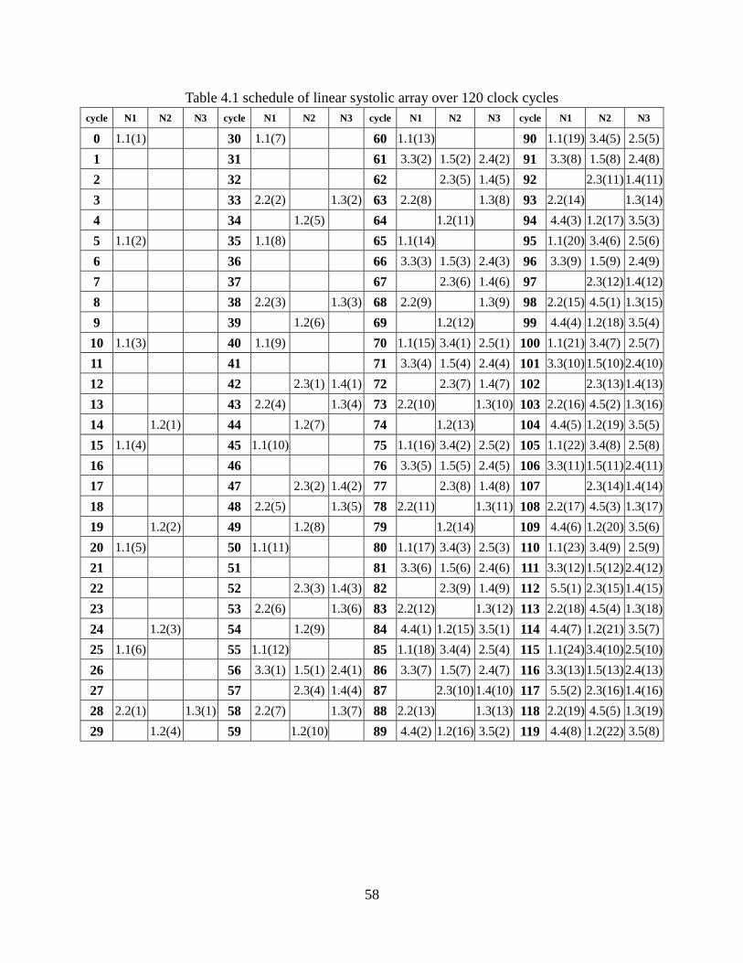
58

Table 4.1 schedule of linear systolic array over 120 clock cycles

cycle N1 N2 N3 cycle N1 N2 N3 cycle N1 N2 N3 cycle N1 N2 N3

0 1.1(1)

30 1.1(7)

60 1.1(13)

90 1.1(19) 3.4(5) 2.5(5)

1

31

61 3.3(2) 1.5(2) 2.4(2) 91 3.3(8) 1.5(8) 2.4(8)

2

32

62

2.3(5) 1.4(5) 92

2.3(11) 1.4(11)

3

33 2.2(2)

1.3(2) 63 2.2(8)

1.3(8) 93 2.2(14)

1.3(14)

4

34

1.2(5)

64

1.2(11)

94 4.4(3) 1.2(17) 3.5(3)

5 1.1(2)

35 1.1(8)

65 1.1(14)

95 1.1(20) 3.4(6) 2.5(6)

6

36

66 3.3(3) 1.5(3) 2.4(3) 96 3.3(9) 1.5(9) 2.4(9)

7

37

67

2.3(6) 1.4(6) 97

2.3(12) 1.4(12)

8

38 2.2(3)

1.3(3) 68 2.2(9)

1.3(9) 98 2.2(15) 4.5(1) 1.3(15)

9

39

1.2(6)

69

1.2(12)

99 4.4(4) 1.2(18) 3.5(4)

10 1.1(3)

40 1.1(9)

70 1.1(15) 3.4(1) 2.5(1) 100 1.1(21) 3.4(7) 2.5(7)

11

41

71 3.3(4) 1.5(4) 2.4(4) 101 3.3(10) 1.5(10) 2.4(10)

12

42

2.3(1) 1.4(1) 72

2.3(7) 1.4(7) 102

2.3(13) 1.4(13)

13

43 2.2(4)

1.3(4) 73 2.2(10)

1.3(10) 103 2.2(16) 4.5(2) 1.3(16)

14

1.2(1)

44

1.2(7)

74

1.2(13)

104 4.4(5) 1.2(19) 3.5(5)

15 1.1(4)

45 1.1(10)

75 1.1(16) 3.4(2) 2.5(2) 105 1.1(22) 3.4(8) 2.5(8)

16

46

76 3.3(5) 1.5(5) 2.4(5) 106 3.3(11) 1.5(11) 2.4(11)

17

47

2.3(2) 1.4(2) 77

2.3(8) 1.4(8) 107

2.3(14) 1.4(14)

18

48 2.2(5)

1.3(5) 78 2.2(11)

1.3(11) 108 2.2(17) 4.5(3) 1.3(17)

19

1.2(2)

49

1.2(8)

79

1.2(14)

109 4.4(6) 1.2(20) 3.5(6)

20 1.1(5)

50 1.1(11)

80 1.1(17) 3.4(3) 2.5(3) 110 1.1(23) 3.4(9) 2.5(9)

21

51

81 3.3(6) 1.5(6) 2.4(6) 111 3.3(12) 1.5(12) 2.4(12)

22

52

2.3(3) 1.4(3) 82

2.3(9) 1.4(9) 112 5.5(1) 2.3(15) 1.4(15)

23

53 2.2(6)

1.3(6) 83 2.2(12)

1.3(12) 113 2.2(18) 4.5(4) 1.3(18)

24

1.2(3)

54

1.2(9)

84 4.4(1) 1.2(15) 3.5(1) 114 4.4(7) 1.2(21) 3.5(7)

25 1.1(6)

55 1.1(12)

85 1.1(18) 3.4(4) 2.5(4) 115 1.1(24) 3.4(10) 2.5(10)

26

56 3.3(1) 1.5(1) 2.4(1) 86 3.3(7) 1.5(7) 2.4(7) 116 3.3(13) 1.5(13) 2.4(13)

27

57

2.3(4) 1.4(4) 87

2.3(10) 1.4(10) 117 5.5(2) 2.3(16) 1.4(16)

28 2.2(1)

1.3(1) 58 2.2(7)

1.3(7) 88 2.2(13)

1.3(13) 118 2.2(19) 4.5(5) 1.3(19)

29

1.2(4)

59

1.2(10)

89 4.4(2) 1.2(16) 3.5(2) 119 4.4(8) 1.2(22) 3.5(8)

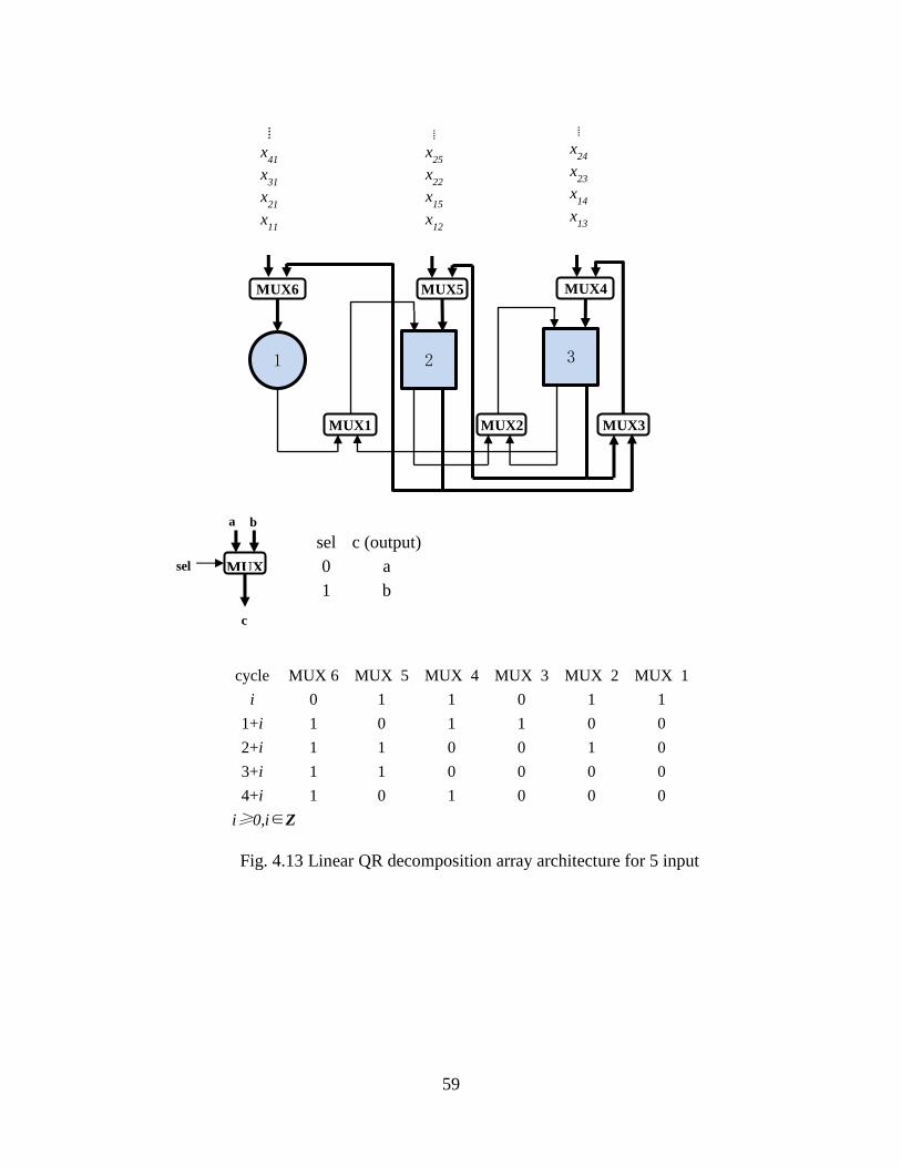
59

2 3 1

MUX6

MUX5

MUX4

MUX1

MUX2

MUX3

⁞

x25

x22

x15

x12

⁞

x24

x23

x14

x13

⁞

x41

x31

x21

x11

Fig. 4.13 Linear QR decomposition array architecture for 5 input

channels

cycle MUX 6 MUX 5 MUX 4 MUX 3 MUX 2 MUX 1

i 0 1 1 0 1 1

1+i 1 0 1 1 0 0

2+i 1 1 0 0 1 0

3+i 1 1 0 0 0 0

4+i 1 0 1 0 0 0

i≥0,i∈Z

sel c (output)

0 a

1 b

MUX

a b

c

sel

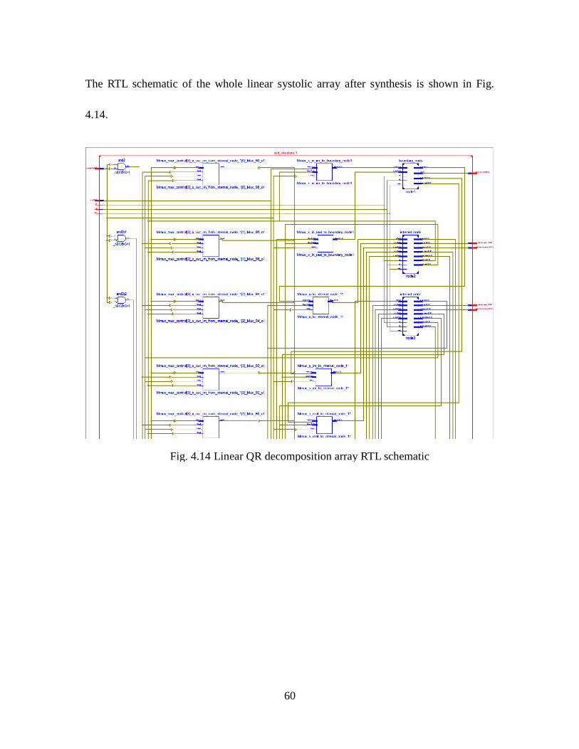
60

The RTL schematic of the whole linear systolic array after synthesis is shown in Fig.

4.14.

Fig. 4.14 Linear QR decomposition array RTL schematic

61

5. RESULT AND PERFORMANCE ANALYSIS

These two kind of systolic arrays were implemented under Xilinx ISE design suit by

customized Verilog code and Xilinx IP core including Multiplier, Adder, Block memory

generator, ChipScope and a Digital clock manger (DCM) IP core. The test matrices were

built into ROM core within design files. All the behavioral simulation and post-route

simulation were done in Modelsim. The ChipScope was used by capture the output upper

triangular matrix value after the bit stream loaded into Xilinx ML605 Virtex6 xc6vlx240t

development board. The hardware test bench is shown in Fig.5.1. The main clock came

from on board 200MHz differential clock. DCM used 200MHz source to generate the

desired clock frequency to drive the whole structure. The control keys outside FPGA

were “reset” and “start” buttons which are used for starting the QR-D and resetting

everything. Status LEDs were used for observing the “running”, “stop” and “idle” status

of the QR-D. The software based analyzer was used for capturing the result data matrices.

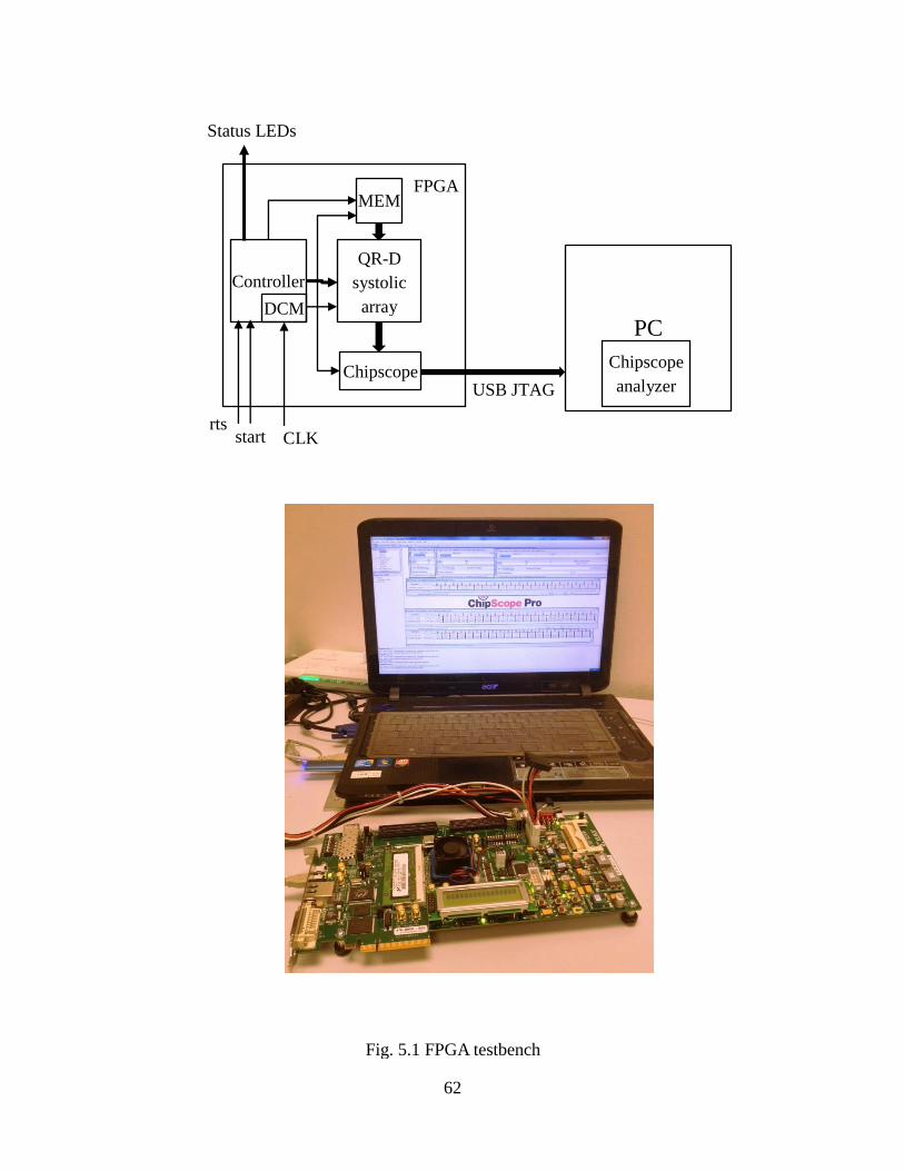
62

MEM

QR-D

systolic

array

Controller

DCM

Chipscope

CLK rts

Chipscope

analyzer

PC

USB JTAG

FPGA

Status LEDs

Fig. 5.1 FPGA testbench

start

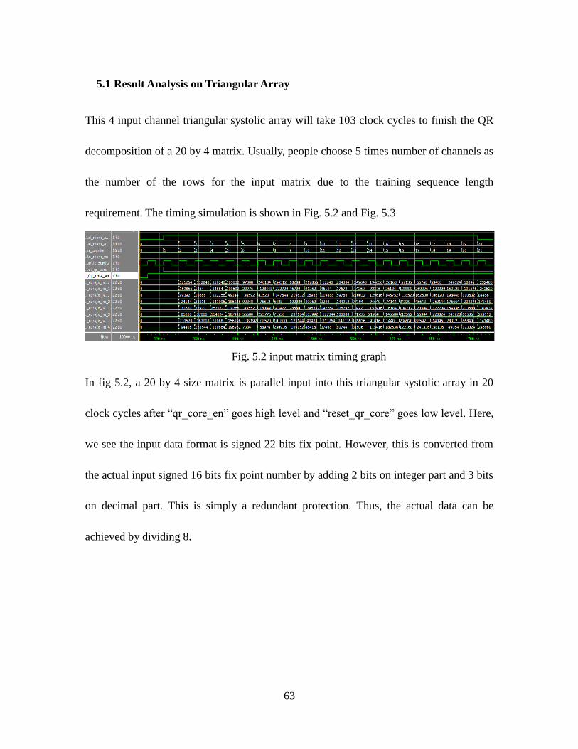
63

Result Analysis on Triangular Array 5.1

This 4 input channel triangular systolic array will take 103 clock cycles to finish the QR

decomposition of a 20 by 4 matrix. Usually, people choose 5 times number of channels as

the number of the rows for the input matrix due to the training sequence length

requirement. The timing simulation is shown in Fig. 5.2 and Fig. 5.3

In fig 5.2, a 20 by 4 size matrix is parallel input into this triangular systolic array in 20

clock cycles after “qr_core_en” goes high level and “reset_qr_core” goes low level. Here,

we see the input data format is signed 22 bits fix point. However, this is converted from

the actual input signed 16 bits fix point number by adding 2 bits on integer part and 3 bits

on decimal part. This is simply a redundant protection. Thus, the actual data can be

achieved by dividing 8.

Fig. 5.2 input matrix timing graph

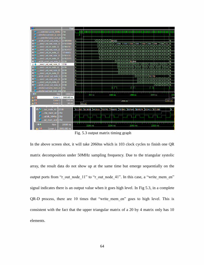
64

In the above screen shot, it will take 2060ns which is 103 clock cycles to finish one QR

matrix decomposition under 50MHz sampling frequency. Due to the triangular systolic

array, the result data do not show up at the same time but emerge sequentially on the

output ports from “r_out_node_11” to “r_out_node_41”. In this case, a “write_mem_en”

signal indicates there is an output value when it goes high level. In Fig 5.3, in a complete

QR-D process, there are 10 times that “write_mem_en” goes to high level. This is

consistent with the fact that the upper triangular matrix of a 20 by 4 matrix only has 10

elements.

Fig. 5.3 output matrix timing graph

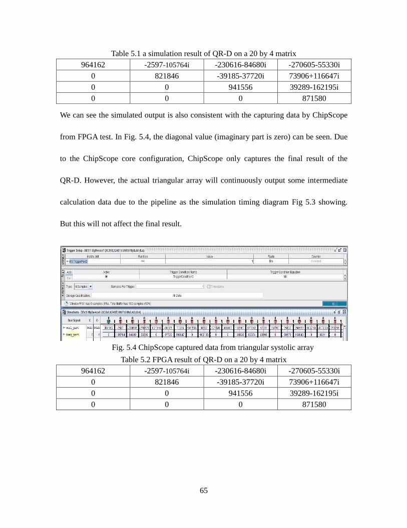
65

Table 5.1 a simulation result of QR-D on a 20 by 4 matrix

964162 -2597-105764i -230616-84680i -270605-55330i

0 821846 -39185-37720i 73906+116647i

0 0 941556 39289-162195i

0 0 0 871580

We can see the simulated output is also consistent with the capturing data by ChipScope

from FPGA test. In Fig. 5.4, the diagonal value (imaginary part is zero) can be seen. Due

to the ChipScope core configuration, ChipScope only captures the final result of the

QR-D. However, the actual triangular array will continuously output some intermediate

calculation data due to the pipeline as the simulation timing diagram Fig 5.3 showing.

But this will not affect the final result.

Table 5.2 FPGA result of QR-D on a 20 by 4 matrix

964162 -2597-105764i -230616-84680i -270605-55330i

0 821846 -39185-37720i 73906+116647i

0 0 941556 39289-162195i

0 0 0 871580

Fig. 5.4 ChipScope captured data from triangular systolic array

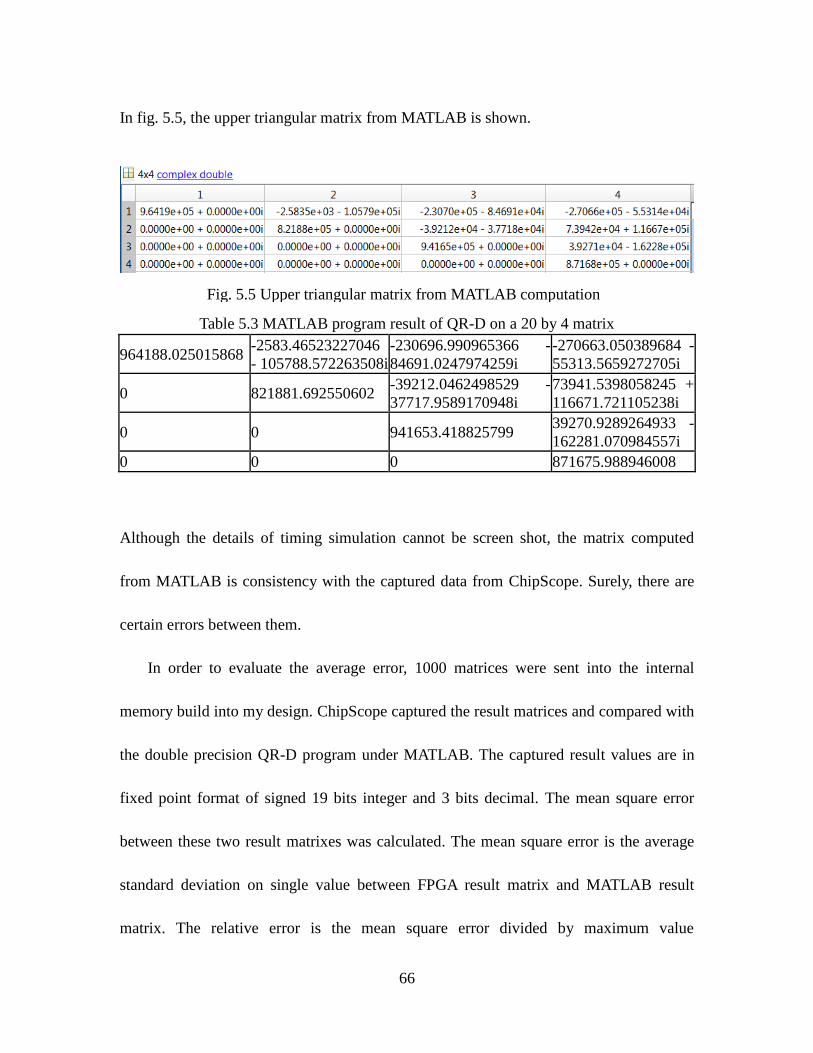
66

In fig. 5.5, the upper triangular matrix from MATLAB is shown.

Table 5.3 MATLAB program result of QR-D on a 20 by 4 matrix

964188.025015868 -2583.46523227046

- 105788.572263508i

-230696.990965366 -

84691.0247974259i

-270663.050389684 -

55313.5659272705i

0 821881.692550602 -39212.0462498529 -

37717.9589170948i

73941.5398058245 +

116671.721105238i

0 0 941653.418825799 39270.9289264933 -

162281.070984557i

0 0 0 871675.988946008

Although the details of timing simulation cannot be screen shot, the matrix computed

from MATLAB is consistency with the captured data from ChipScope. Surely, there are

certain errors between them.

In order to evaluate the average error, 1000 matrices were sent into the internal

memory build into my design. ChipScope captured the result matrices and compared with

the double precision QR-D program under MATLAB. The captured result values are in

fixed point format of signed 19 bits integer and 3 bits decimal. The mean square error

between these two result matrixes was calculated. The mean square error is the average

standard deviation on single value between FPGA result matrix and MATLAB result

matrix. The relative error is the mean square error divided by maximum value

Fig. 5.5 Upper triangular matrix from MATLAB computation

67

represented by the fix-point format. The absolute error is 7.608. The relative error

comparing the maximum value represented by this 22 bits data format is 2.902e-05. Even

though the absolute error seems to be large due to the imperfection of the square root

inverse, it still meets the requirement of the real application.

Dynamic range of an antenna array can be generalized to the value dropping between

Eigenvalue one and Eigenvalue two of the covariance matrix obtained from the received

data matrix. Assume a scenario of single transmitting source. The antenna array will

simply produce a rank one matrix when beamforming is not used. Obtain the covariance

matrix by formula M=XHX where X is the received data matrix. Apply a SVD on this

covariance matrix and find the Eigenvalue distribution. In this distribution, the received

signal energy is mainly on the Eigen one and the other Eigenvalues should be around the

noise floor. Thus, the dynamic range of the received signal can be obtained by evaluating

the Eigen one value.

Therefore, the hardware on the receiver should provide high dynamic range than the

received signal. Based on the reference paper [20] [21], the dynamic range requirement

should be larger than 61dB. Meanwhile, a general 14 bits ADC can provide effective 12

bits which is 12×6=72dB. In this case, the dynamic range requirement should be 72dB.

To test the dynamic range of this linear systolic array, rank one complex matrices with

increasing magnitude but random phase can be sent to the QR-D and then evaluate the

Eigenvalue distribution. By increasing the input magnitude and finding the dropping

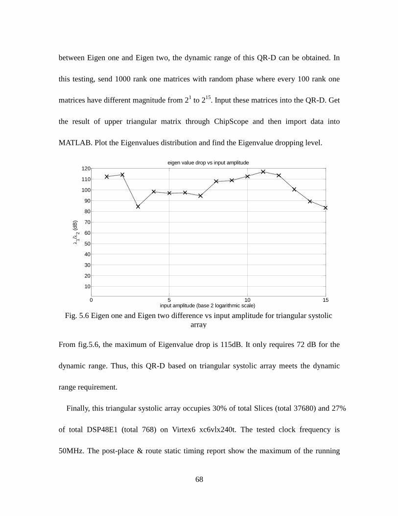
68

between Eigen one and Eigen two, the dynamic range of this QR-D can be obtained. In

this testing, send 1000 rank one matrices with random phase where every 100 rank one

matrices have different magnitude from 21 to 2

15. Input these matrices into the QR-D. Get

the result of upper triangular matrix through ChipScope and then import data into

MATLAB. Plot the Eigenvalues distribution and find the Eigenvalue dropping level.

From fig.5.6, the maximum of Eigenvalue drop is 115dB. It only requires 72 dB for the

dynamic range. Thus, this QR-D based on triangular systolic array meets the dynamic

range requirement.

Finally, this triangular systolic array occupies 30% of total Slices (total 37680) and 27%

of total DSP48E1 (total 768) on Virtex6 xc6vlx240t. The tested clock frequency is

50MHz. The post-place & route static timing report show the maximum of the running

Fig. 5.6 Eigen one and Eigen two difference vs input amplitude for triangular systolic

array

0 5 10 15

10

20

30

40

50

60

70

80

90

100

110

120

input amplitude (base 2 logarithmic scale)

1/

2 (

dB

)

eigen value drop vs input amplitude

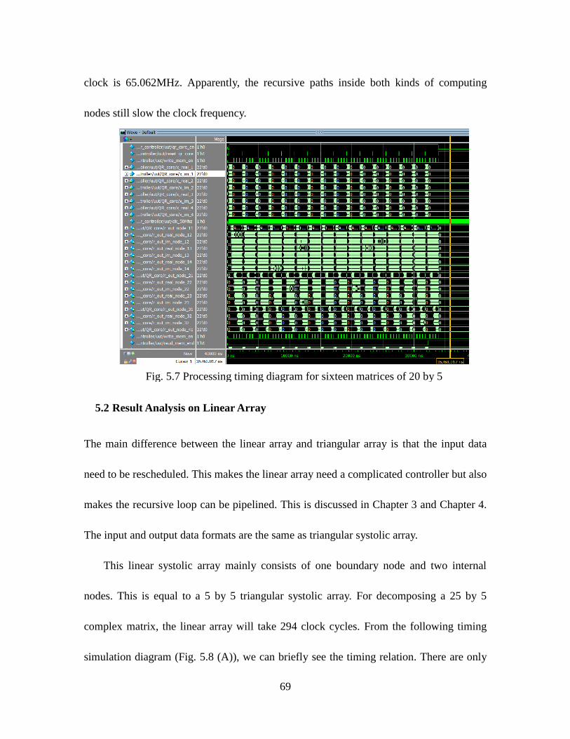
69

clock is 65.062MHz. Apparently, the recursive paths inside both kinds of computing

nodes still slow the clock frequency.

Result Analysis on Linear Array 5.2

The main difference between the linear array and triangular array is that the input data

need to be rescheduled. This makes the linear array need a complicated controller but also

makes the recursive loop can be pipelined. This is discussed in Chapter 3 and Chapter 4.

The input and output data formats are the same as triangular systolic array.

This linear systolic array mainly consists of one boundary node and two internal

nodes. This is equal to a 5 by 5 triangular systolic array. For decomposing a 25 by 5

complex matrix, the linear array will take 294 clock cycles. From the following timing

simulation diagram (Fig. 5.8 (A)), we can briefly see the timing relation. There are only

Fig. 5.7 Processing timing diagram for sixteen matrices of 20 by 5

70

two data input port “x_real” and “x_im” (Fig. 5.8 (B)) connected to the memory stored

the matrices. The controller will pass the values of these two ports to each node by

rescheduling diagram in Table 4.1. The controller also keeps sending the control signal

periodically for all six multiplexers. The control signal is “mux_control” in Fig. 5.8 (C).

These multiplexers are used for exchanging the c s and x_out values among nodes as

Table 4.1 described. In Fig. 5.8 (D), “write_mem_en” is used to tell ChipScope to capture

the output data. “write_mem_en” has a width of 3 and each bit represents the outputting

status on each node.

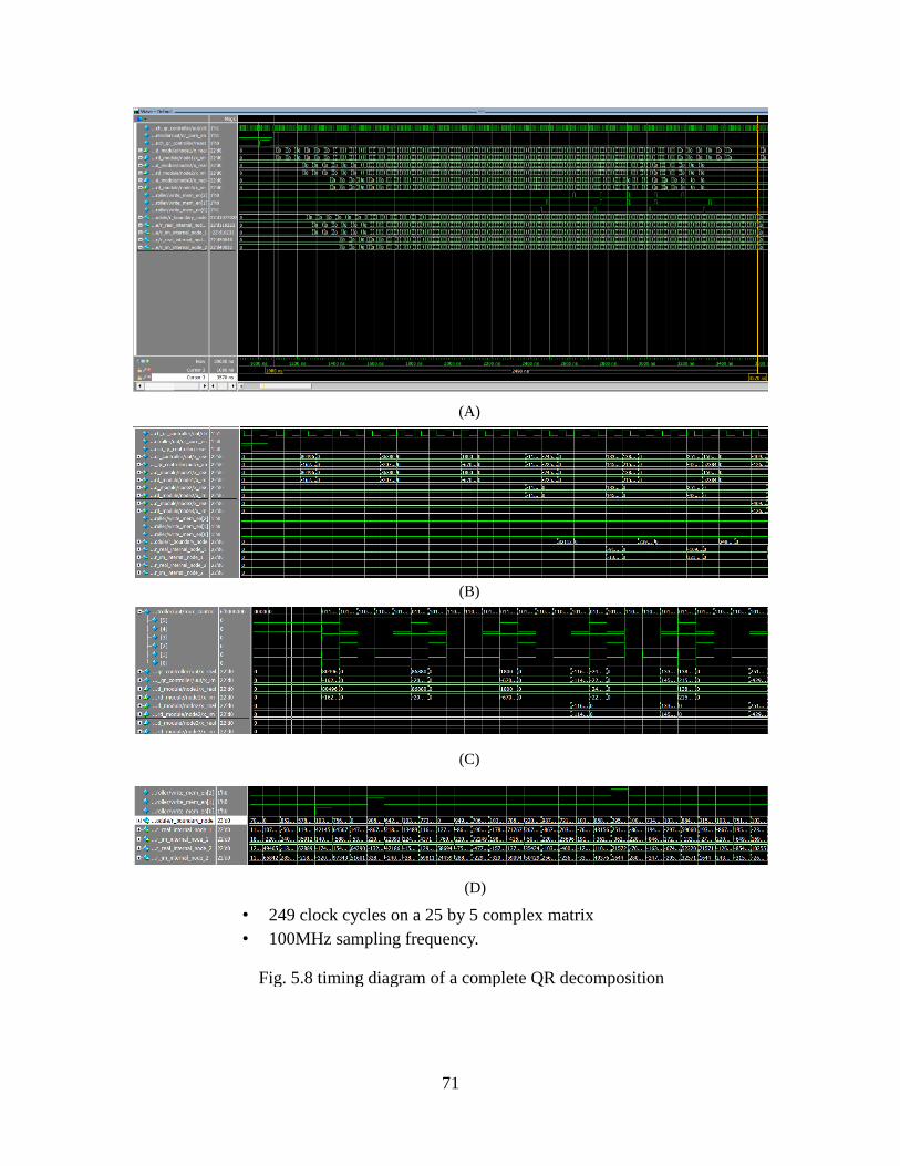
71

Fig. 5.8 timing diagram of a complete QR decomposition

(A)

(B)

(C)

(D)

• 249 clock cycles on a 25 by 5 complex matrix

• 100MHz sampling frequency.

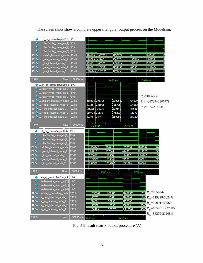
72

The screen shots show a complete upper triangular output process on the Modelsim.

R11=1037532

R12=-86739+220677i

R13=21572+1644i

R22

=1056742

R23

=119328-16247i

R14

=50091+40066i

R15

=185781+227385i

R24

=88279-212084i

Fig. 5.9 result matrix output procedure (A)

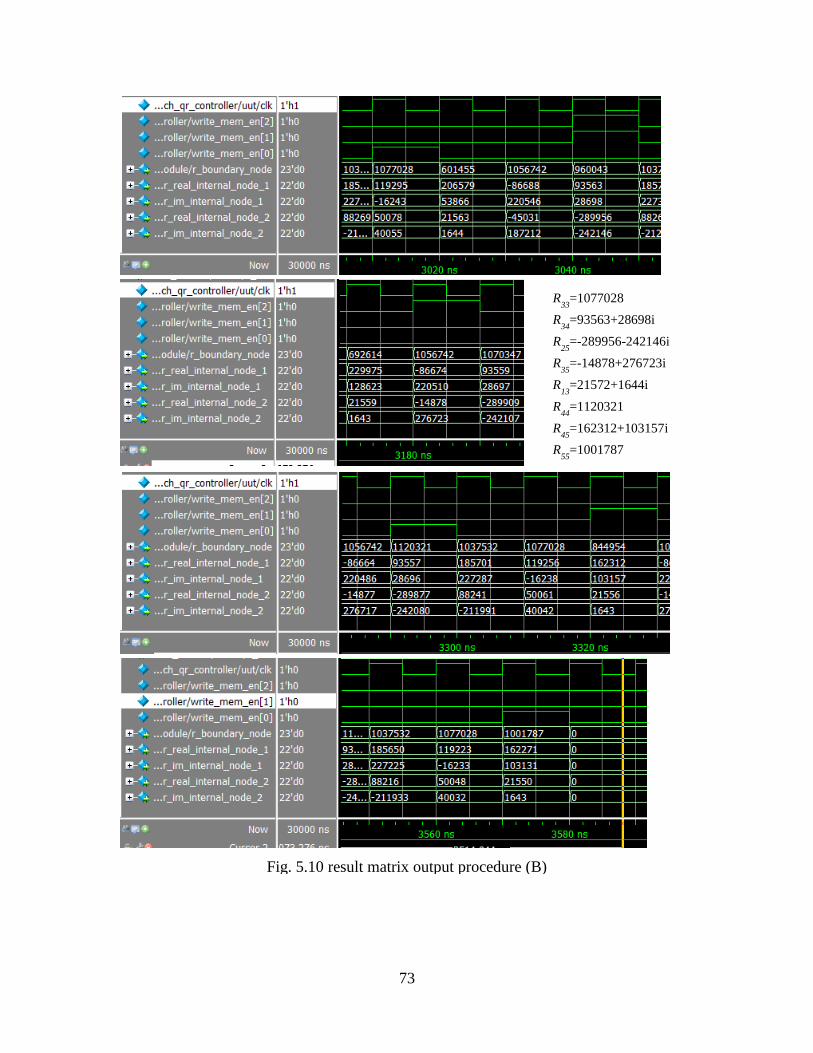
73

R33

=1077028

R34

=93563+28698i

R25

=-289956-242146i

R35

=-14878+276723i

R13

=21572+1644i

R44

=1120321

R45

=162312+103157i

R55

=1001787

Fig. 5.10 result matrix output procedure (B)

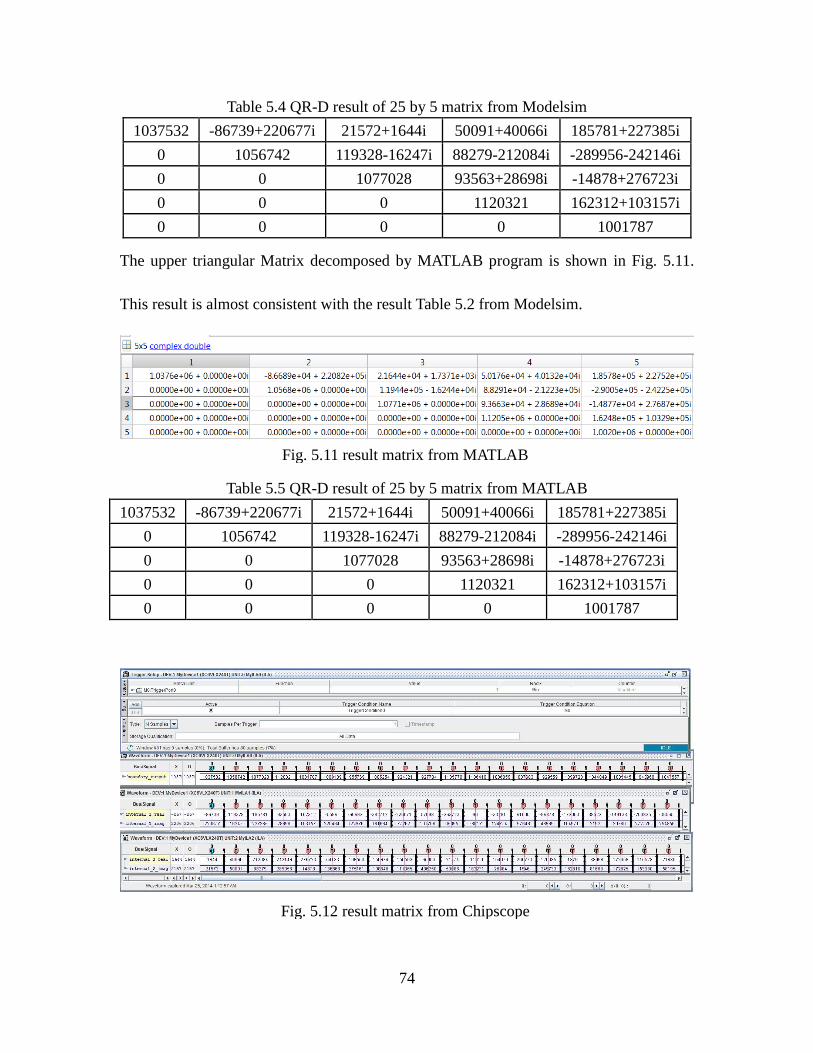
74

Table 5.4 QR-D result of 25 by 5 matrix from Modelsim

1037532 -86739+220677i 21572+1644i 50091+40066i 185781+227385i

0 1056742 119328-16247i 88279-212084i -289956-242146i

0 0 1077028 93563+28698i -14878+276723i

0 0 0 1120321 162312+103157i

0 0 0 0 1001787

The upper triangular Matrix decomposed by MATLAB program is shown in Fig. 5.11.

This result is almost consistent with the result Table 5.2 from Modelsim.

Table 5.5 QR-D result of 25 by 5 matrix from MATLAB

1037532 -86739+220677i 21572+1644i 50091+40066i 185781+227385i

0 1056742 119328-16247i 88279-212084i -289956-242146i

0 0 1077028 93563+28698i -14878+276723i

0 0 0 1120321 162312+103157i

0 0 0 0 1001787

Fig. 5.11 result matrix from MATLAB

Fig. 5.12 result matrix from Chipscope

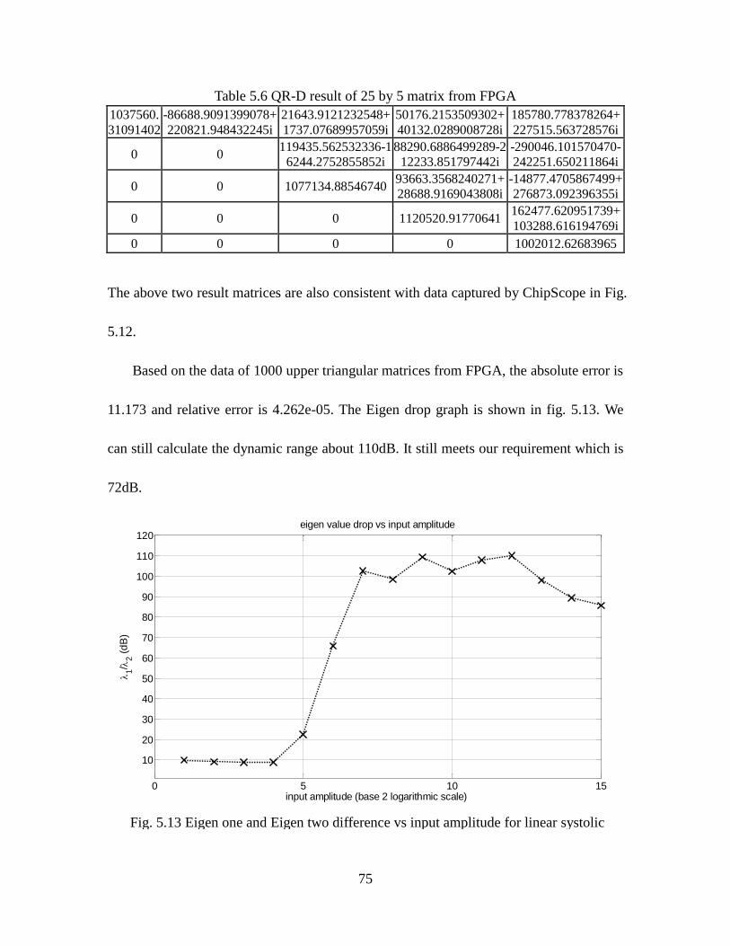
75

Table 5.6 QR-D result of 25 by 5 matrix from FPGA

1037560.

31091402

-86688.9091399078+

220821.948432245i

21643.9121232548+

1737.07689957059i

50176.2153509302+

40132.0289008728i

185780.778378264+

227515.563728576i

0 0 119435.562532336-1

6244.2752855852i

88290.6886499289-2

12233.851797442i

-290046.101570470-

242251.650211864i

0 0 1077134.88546740 93663.3568240271+

28688.9169043808i

-14877.4705867499+

276873.092396355i

0 0 0 1120520.91770641 162477.620951739+

103288.616194769i

0 0 0 0 1002012.62683965

The above two result matrices are also consistent with data captured by ChipScope in Fig.

5.12.

Based on the data of 1000 upper triangular matrices from FPGA, the absolute error is

11.173 and relative error is 4.262e-05. The Eigen drop graph is shown in fig. 5.13. We

can still calculate the dynamic range about 110dB. It still meets our requirement which is

72dB.

Fig. 5.13 Eigen one and Eigen two difference vs input amplitude for linear systolic

array

0 5 10 15

10

20

30

40

50

60

70

80

90

100

110

120

input amplitude (base 2 logarithmic scale)

1/

2 (

dB

)

eigen value drop vs input amplitude

76

Finally, this linear systolic array occupies 12% of total Slices (total 37680) and 7% of

total DSP48E1 (total 768) on Virtex6 xc6vlx240t. The tested clock frequency is 100MHz.

The post-place & route static timing report show the maximum of the running clock is

135.373MHz. The tested clock frequency is 100MHz. Compared with the triangular array,

it certainly consumes less FPGA logical resources and runs at higher clock frequency,

which means a higher data sample rate. But it sacrifices the parallelism of the triangular

array. This linear array can provide maximum data throughput is almost 2Gbit/sec. The

triangular array can provide maximum data throughput is almost 4Gbits/sec. Although the

triangular systolic array seems to have higher data throughput, its recursive loops of

triangular systolic cannot be pipelined and this bottleneck cannot be easily broken

through. The linear array can still be added more pipeline stages to increase the clock

frequency and consumes much smaller resources when the data matrix becomes larger.

Therefore, linear systolic will be the best choice for the future work.

77

6. CONCLUSION AND FUTURE WORK

Conclusion 6.1

Based on the result analysis on Chapter 5, the dynamic range of both triangular array and

linear array can meet the requirement which is 72dB. However, the sampling frequency

(equal to system clock frequency in this report) is not very high. The triangular array has

a maximum clock frequency of 65MHz and 4 parallel input channels. The linear array has

a higher maximum clock frequency which is 135MHz but only one input channel. For the

common communication system, this sampling frequency may be not a problem. But for

many wideband systems like phased array radar, the QR-D implemented on this thesis

still needs more modification to increase the sampling frequency. Meanwhile, more

accurate floating-point arithmetic will also be part of the next goal for this QR-D.

Future Work 6.2

For the adaptive beamforming array, QR decomposition processors array does not only

work on matrix triangularization but also computes the beamforming weight. The QR

decomposition implemented in this thesis can also be developed furthermore to fulfill

weight computation. Fig 6.1 introduces the general method for beamforming weight

computation. Constraints (steering vector) should be added to the decomposed triangular

matrix. Then a double back-substitution is needed.

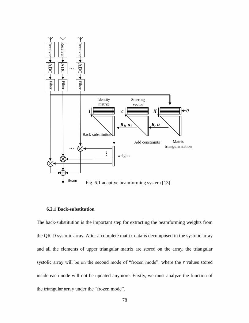
78

6.2.1 Back-substitution

The back-substitution is the important step for extracting the beamforming weights from

the QR-D systolic array. After a complete matrix data is decomposed in the systolic array

and all the elements of upper triangular matrix are stored on the array, the triangular

systolic array will be on the second mode of “frozen mode”, where the r values stored

inside each node will not be updated anymore. Firstly, we must analyze the function of

the triangular array under the “frozen mode”.

AD

C

AD

C

I X 0

c

Steering

vector

R, u

Identity

matrix

R1, u1

weights

AD

C

Receiv

er

Receiv

er

Receiv

er

Filter

F

ilter

Filter

Matrix

triangularization Add constraints

Back-substitution

…

… …

Beam

Fig. 6.1 adaptive beamforming system [13]

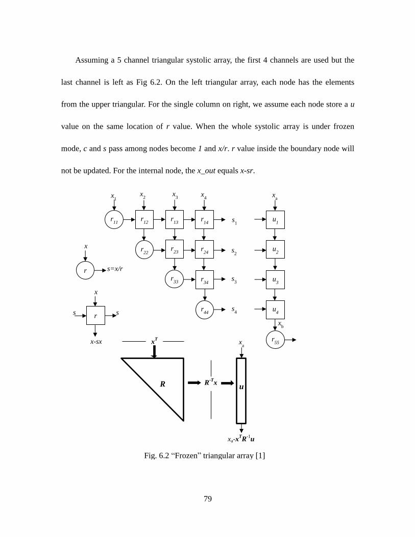
79

Assuming a 5 channel triangular systolic array, the first 4 channels are used but the

last channel is left as Fig 6.2. On the left triangular array, each node has the elements

from the upper triangular. For the single column on right, we assume each node store a u

value on the same location of r value. When the whole systolic array is under frozen

mode, c and s pass among nodes become 1 and x/r. r value inside the boundary node will

not be updated. For the internal node, the x_out equals x-sr.

xa

r55

u1

u2

u3

u4

xb

x1 x

2

r11 r

12 r

13 r

14

r22 r

23 r

24

r33 r

34

r44

x3 x

4

s1

s2

s3

s4

r

x

s=x/r

r s s

x

x-sx

Fig. 6.2 “Frozen” triangular array [1]

R u

xT

R-T

x

xa

xa-xTR

-1u

80

In Fig 6.2, for the triangular array, we can follow the relations, for example, [1]

1 1 11 2 2 12 1 22

3 3 13 1 23 2 33

/ /

/

s x r s x r s r

s x r s r s r

, (6.1)

Then

1 11 1 2 12 1 22 2

3 13 1 23 2 33 3

x r s x r s r s

x r s r s r s

. (6.2)

Apparently [1]

T

T

R s x

s R x , (6.3)

For the column array on right in Fig 6.2, if we input the s vector into the this column

array, we can get

1 1 2 2 3 3 4 4

1

b a

T

b a

T

b a

x x u s u s u s u s

x x

x x

s u

x R u

. (6.4)

Furthermore, if we input a matrix X instead of vector x and a vector xb instead of a scale

xb. We can get [1]

1T

b a

x x X R u . (6.5)

If input an identity matrix on X and zeroes vector on xa, we get

1

b

x R u . (6.6)

In fact, this is our weights output, but that detail will be discussed in next section.

Therefore, for this 5 by 5 triangular array, we can simply get our weights flushed serially

by inputting a 4 by 4 identity matrix to the first 4 channels and a zeroes vector to the last

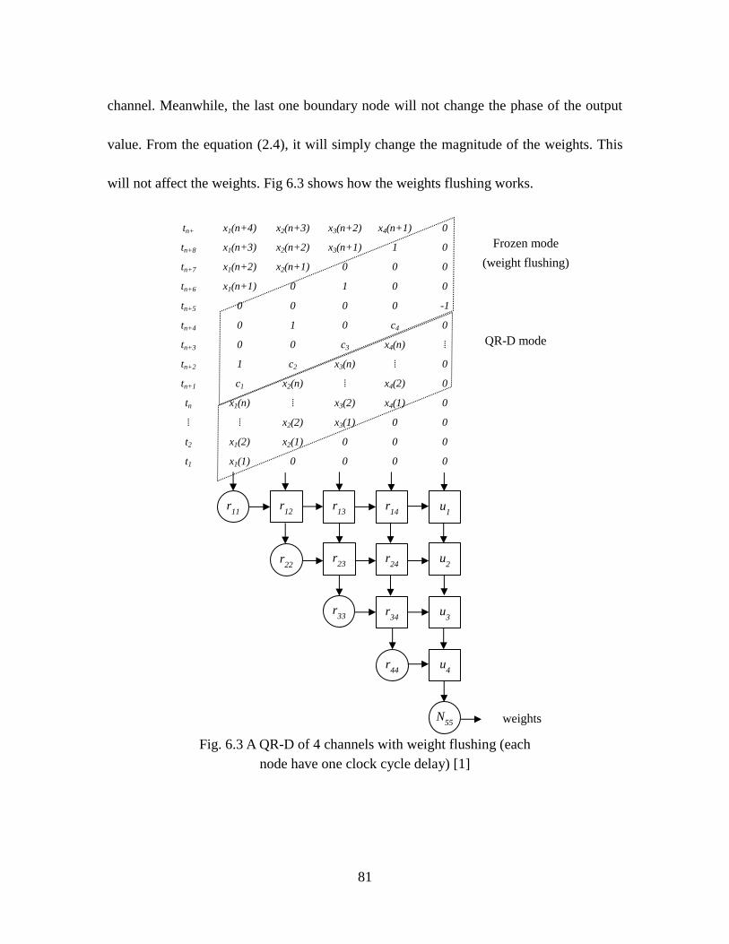
81

channel. Meanwhile, the last one boundary node will not change the phase of the output

value. From the equation (2.4), it will simply change the magnitude of the weights. This

will not affect the weights. Fig 6.3 shows how the weights flushing works.

tn+ x1(n+4) x2(n+3) x3(n+2) x4(n+1) 0

tn+8 x1(n+3) x2(n+2) x3(n+1) 1 0

tn+7 x1(n+2) x2(n+1) 0 0 0

tn+6 x1(n+1) 0 1 0 0

tn+5 0 0 0 0 -1

tn+4 0 1 0 c4 0

tn+3 0 0 c3 x4(n) ⁞

tn+2 1 c2 x3(n) ⁞ 0

tn+1 c1 x2(n) ⁞ x4(2) 0

tn x1(n) ⁞ x3(2) x4(1) 0

⁞ ⁞ x2(2) x3(1) 0 0

t2 x1(2) x2(1) 0 0 0

t1 x1(1) 0 0 0 0

Fig. 6.3 A QR-D of 4 channels with weight flushing (each

node have one clock cycle delay) [1]

r11 r

12 r

13 r

14 u

1

r22 r

23 r

24 u

2

r33 r

34 u

3

r44 u

4

N55

QR-D mode

Frozen mode

(weight flushing)

weights

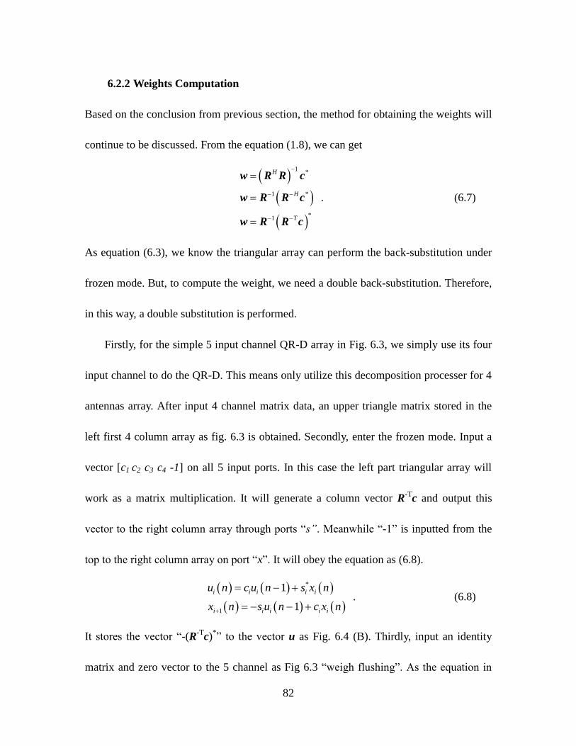
82

6.2.2 Weights Computation

Based on the conclusion from previous section, the method for obtaining the weights will

continue to be discussed. From the equation (1.8), we can get

1*

1 *

*1

H

H

T

w R R c

w R R c

w R R c

. (6.7)

As equation (6.3), we know the triangular array can perform the back-substitution under

frozen mode. But, to compute the weight, we need a double back-substitution. Therefore,

in this way, a double substitution is performed.

Firstly, for the simple 5 input channel QR-D array in Fig. 6.3, we simply use its four

input channel to do the QR-D. This means only utilize this decomposition processer for 4

antennas array. After input 4 channel matrix data, an upper triangle matrix stored in the

left first 4 column array as fig. 6.3 is obtained. Secondly, enter the frozen mode. Input a

vector [c1 c2 c3 c4 -1] on all 5 input ports. In this case the left part triangular array will

work as a matrix multiplication. It will generate a column vector R-T

c and output this

vector to the right column array through ports “s”. Meanwhile “-1” is inputted from the

top to the right column array on port “x”. It will obey the equation as (6.8).

*

1

1

1

i i i i i

i i i i i

u n c u n s x n

x n s u n c x n

. (6.8)

It stores the vector “-(R-T

c)*” to the vector u as Fig. 6.4 (B). Thirdly, input an identity

matrix and zero vector to the 5 channel as Fig 6.3 “weigh flushing”. As the equation in

83

(6.5) (6.6), the weight can be calculated as equation (6.7).

*,( ), T

a -cX R xI u 0 . (6.9)

Bringing the above variables to equation (6.5), obtain the exact same express as equation

(6.7) as in Fig 6.4 (C). Then the w vector will go through the last boundary node where

magnitude will be changed but phase of weights will keep the same. Finally, we extract

the weight from the QR-D triangular array. For the linear systolic array, everything is the

same.

R u

xT

R-T

x

xa

xa-x

T

R-1

u

(A)

R

u

cT

R-T

c

-1

=-(R-T

c)*

(B) w=0-I

T

R-1

(-R-T

c)*

= R-1

(R-T

c)*

R

u

I

R-T

I

0

=-(R-T

c)*

(C)

Fig. 6.4 Weights computing processing

84

REFERENCES

1. T.J Shephard and J.G. McWhirter, “Systolic adaptive beamforming” Chapter. 5, Array

Processing, S. Haykin, J. Litva and T.J. Shephard (Eds.), Springer-Verlag, ISBN

3-540-55224, 1993, pp. 153-243.

2. G. Lightbody, R. L. Walke, R. Woods, J. McCanny, “Linear QR Architecture for a

Single Chip Adaptive Beamformer”, Journal of VLSI Signal Processing, Vol. 24, pp.

67-81, 2000.

3. S. Y. Kung, VLSI Array Processors, Prentice Hall, ISBN 0-13-942749-X, 1988.

4. Gene H. Golub, Charles F. Van Loan, Matrix Computations (3rd Edition), Johns

Hopkins University Press, ISBN-13: 978-0801854149

5. Huy Nguyen, James Haupt, Michael Eskowitz, Birol Bekirov, Jonathan Scalera,

Thomas Anderson, Michael Vai, and Kenneth Teitelbaum, “High-Performance

FPGA-Based QR Decomposition”, High Performance Embedded Computing

Workshop, 2005.

6. W. Givens, “Computation of Plane Unitary Rotations Transforming a General Matrix

to Triangular Form”, J. Soc. Indust. Appl. Math., Vol. 6, No. 1, pp. 26-50, March

1958.

7. G. H. Golub, “Numerical methods for solving linear least-squares problems” Num.

Math., no. 7, pp. 206-216, 1965.

8. C. R. Ward, P. J. Hargrave, and J. G. McWhirter, “A Novel Algorithm and

Architecture for Adaptive Digital Beamforming”, IEEE Trans. on Antennas and

Propagation, Vol. AP-34, No. 3, pp. 338-346, March 1986.

9. J. G. McWhirter, “Recursive least-squares minimization using a systolic array”, Proc.

SPIE 431, Real-Time Signal Processing VI, pp. 105-112, 1983.

10. W. M. Gentleman and H. T. Kung, “Matrix triangularization by systolic arrays”, Proc.

SPIE 298, Real-Time Signal Processing IV, pp. 19-26, 1981.

11. X. Wang, Airvana and M. Leeser, “A Truly Two-Dimensional Systolic Array FPGA

Implementation of QR Decomposition” ACM Transaction on Embedded Computing

System, Vol. 9, No. 1 Article 3, October 2009

85

12. W. M. Gentleman, “Least-squares computations by Givens transformations without

square roots”, J. Inst. Math. Its Appl. 12, 329-336(1973)

13. R.L. Walke, R. W. M. Smith and G. Lightbody “20 GFLOPS QR processor on a

Xilinx Virtex-E FPGA”, SPIE Vol. 4116 (2000) © 2000 SPIE

14. G. Lightbody, R. L. Walke, R. Woods, J. McCanny, “Novel Mapping of a Linear QR

Architecture”, Proc. ICASSP, vol. IV, pp. 1933-6, 1999.

15. J.G. McWhirter, R.L.Walke, and J. Kadlec, “Normalized givens rotations for

recursive least squares processing,” VLSI Signal Processing, VIII, .ISBN

0-7803-2612-1, pp. 323–332, 1995.

16. R. Walke, R. W. M. Smith and G. Lightbody, “Architectures for Adaptive Weight

Calculation on ASIC and FPGA”, Proc. 33rd Asilomar Conference on Signals,

Systems and Computers, 1999.

17. R.L. Walke, “High sample rate givens rotations for recursive least squares,” Ph.D.

Thesis, University of Warwick, 1997.

18. Altera, “QR Matrix Decomposition”, reference design.

http://www.altera.com/literature/an/an506.pdf

19. Walke, R., “Adaptive Beamforming Using QR in FPGA,” High Performance

Embedded Computing Workshop, 2002.

20. Shawn Kraut, Adam R. Margetts and Daniel W. Bliss, “Reducing the Fractional Rank

of Interference with Space-Time-Frequency Adaptive Beamforming” Asilomar

Conference. 2013

21. D. W. Bliss, P. A. Parker, A. R. Margetts, “Simultaneous Transmission And Reception

For Improved wireless Network Performance” Statistical Signal Processing, 2007.

SSP '07. IEEE/SP 14th Workshop on

22. J. Volder, “The CORDIC Trigonometric Computing Technique” IRE Trans. Electron.

Comput., Vol. EC-8, pp. 330-334, 1959

23. Michael Gay and Isabel Phillips, QinetiQ Ltd. “Real-Time Adaptive Beamforming:

86

FPGA implementation Using QR Decomposition” JED, The JOURNAL of

ELECTRONIC DEFENSE • SEPTEMBER'05

24. B. Yang, J.F. Bohme, “systolic implementation of a general adaptive array processing

algorithm”, Proc. 1988 IEEE Int. Conf. on Acoustic, Speech, and Signal Processing,

New York (1988) pp. 2785-2789

25. M-J. Chen, K. Yao “Linear systolic array for least square estimation” in Proc. Int.

Conf. on Systolic arrays, Computer Society Press, Washington, DC 1988

26. C. M. Rader “wafer-scale systolic array for adaptive antenna processing” Proc. 1988

IEEE Int. Conf. on Acoustic, Speech, and Signal Processing, New York (1988) pp.

2069-2071

27. Daniel W. Bliss, Siddhartan Govindasamy Adptive wireless communications: MIMO

channels and networks Cambridge University Press, ISBN 978-1-107-03320-7, 2013

Documents

FPGA-Based Implementation of QR Decomposition … Implementation of QR Decomposition by ... A Thesis Presented in Partial Fulfillment ... is the estimated p by p covariance matrix