Fourth Review of PJM’s Variable

Fourth Review of PJM’s Variable

Resource Requirement Curve

PREPARED FOR

PREPARED BY

Samuel A. Newell

David Luke Oates

Johannes P. Pfeifenberger

Kathleen Spees

J. Michael Hagerty

John Imon Pedtke

Matthew Witkin

Emily Shorin

April 19, 2018

Acknowledgements: The authors would like to thank PJM staff for their cooperation and

responsiveness to our many questions and requests. We would also like to thank the PJM

Independent Market Monitor for helpful discussions. Opinions expressed in this report, as well

as any errors or omissions, are the authors’ alone.

Copyright © 2018 The Brattle Group, Inc.

i | brattle.com

Table of Contents

Executive Summary ....................................................................................................................... iii

I. Background .............................................................................................................................. 13

A. Study Purpose and Scope ................................................................................................... 13

B. Overview of PJM’s Reliability Pricing Model ................................................................... 14

C. Description of the Variable Resource Requirement Curve .............................................. 15

II. Net Cost of New Entry Parameter ........................................................................................... 17

A. Updated Gross CONE Estimates ........................................................................................ 17

B. Net E&AS Revenue Offset.................................................................................................. 19

1. PJM’s Peak-Hour Dispatch Against Historical Prices ............................................. 20

2. Option for a Forward-Looking E&AS Offset Approach ......................................... 25

C. Indicative Net CONE Estimates ......................................................................................... 29

D. Construction of “RTO-Wide” Net CONE for the System VRR Curve ............................ 31

E. Choice of Reference Technology ....................................................................................... 32

III. Probabilistic Simulation Approach .......................................................................................... 35

A. Model Structure .................................................................................................................. 35

B. Demand Modeling .............................................................................................................. 36

C. Supply Modeling ................................................................................................................. 37

1. Supply Entry, Exit, and Offer Prices ....................................................................... 37

2. Supply Curve Adjustments for Capacity Performance ........................................... 41

D. Reliability Outcomes .......................................................................................................... 46

E. Fluctuations in Supply, Demand, and Transmission ........................................................ 47

F. Summary of Base Case Parameters and Input Assumptions............................................. 50

IV. System-Wide Variable Resource Requirement Curve ............................................................. 51

A. System-Wide Design Objectives ........................................................................................ 52

B. Qualitative Review of the Current System Curve ............................................................ 55

1. Downward-Sloping, Convex Shape ......................................................................... 55

2. Quantity at the Cap .................................................................................................. 56

3. VRR Curve Width .................................................................................................... 58

C. Simulated Performance With Prior Net CONE and Market Entry Price ....................... 59

1. Effect of Capacity Performance ............................................................................... 60

2. Sensitivity to Uncertainties in Capacity Performance and Fluctuations ............... 60

3. Re-Evaluation of the Left-Shift of the VRR Curve ................................................. 62

D. Simulated Performance With Updated Net CONE .......................................................... 63

ii | brattle.com

1. Simulated Performance of Candidate Curves ......................................................... 64

2. Alternative Price Cap with a CC Reference Resource ........................................... 67

E. Summary and Recommendations for the System-Wide VRR Curve .............................. 69

V. Locational Variable Resource Requirement Curves ................................................................. 70

A. Summary of Locational Reliability Requirement ............................................................. 70

B. Qualitative Review of Locational Curves .......................................................................... 71

1. LDA Net CONE ........................................................................................................ 71

2. Locational Curve Price Cap and Shape .................................................................... 72

3. Locational Curve Width ........................................................................................... 73

C. Simulated Performance of System Curves Applied Locally ............................................. 76

1. Performance under Base Case Assumptions ........................................................... 77

2. Performance with Net CONE Higher than Parent ................................................. 77

3. Sensitivity to Primary Modeling Uncertainties ...................................................... 80

4. Sensitivity to Administrative Errors in Net CONE ................................................. 82

D. Recommendations for Locational VRR Curves ................................................................ 83

List of Acronyms ............................................................................................................................ 87

Bibliography ................................................................................................................................... 89

Appendix A: Magnitude of Monte Carlo Fluctuations ................................................................... 95

A. Supply Offer Quantity ........................................................................................................ 95

B. Reliability Requirement ..................................................................................................... 96

C. Administrative Net CONE ................................................................................................. 98

D. Capacity Emergency Transfer Limit ................................................................................ 100

E. Net Supply ......................................................................................................................... 102

Appendix B: Supply Curves with Capacity Performance ............................................................. 104

A. Expected Performance Hours .......................................................................................... 105

B. Supply Curves Under Capacity Performance .................................................................. 108

iii | brattle.com

Executive Summary

The Brattle Group has been commissioned to conduct the Quadrennial Review of the Variable

Resource Requirement (VRR) curve that PJM uses in its capacity market, the Reliability Pricing

Model (RPM). Periodic reviews of VRR curve parameters help ensure that the RPM continues to

support reliability objectives cost-effectively even as market fundamentals and technologies

change. The present review will inform PJM’s filing establishing the VRR curve for the next

four capacity auctions, subject to annual updates. Consistent with the requirements in PJM’s

Tariff, our review analyzes the Net Cost of New Entry (Net CONE) and the VRR curve shape.

High-Level Conclusions and Recommendations

Net CONE represents the capacity revenue a new generator would need to be willing to enter

the market. It reflects the levelized investment and fixed costs (or CONE) of an economic

reference technology, minus expected net energy and ancillary service (E&AS) revenues. We

estimate CONE values for natural gas-fired simple-cycle combustion turbines (CTs) and

combined-cycles (CCs) in a concurrently-filed report.1 This report evaluates PJM’s E&AS

estimation methodology and combines the components into indicative estimates of Net CONE.

The conclusions from our Net CONE analysis are:

1. The updated estimate of Net CONE for CT plants—the current reference technology for the

VRR curve as specified in PJM’s tariff—is 25-42% lower than PJM’s 2021/22 Net CONE

parameters, depending on location.2 The decline is driven by increased economies of scale of

new H-class CTs, a lower tax rate, and a slightly lower cost of capital.

2. The updated estimate of Net CONE for CC plants—the dominant technology of new

generation in PJM for more than fifteen years—is 44-76% lower than PJM’s 2021/22 Net

CONE parameters, and 25-63% below our updated CT Net CONE estimates, depending on

location. CCs are more economic because their much higher net E&AS revenues more than

offset slightly higher plant costs on a per-kW basis.

3. We propose: (a) relatively minor changes to how historical E&AS offsets are calculated for

CTs; (b) a method for estimating forward-looking E&AS offsets for CCs based on futures

settlement prices; and (c) a modified calculation of the RTO-wide value for Net CONE.

The shape of PJM’s current VRR curve is a piecewise-linear “kinked” curve that is convex below

the cap and centered approximately on a quantity defined by the installed reserve margin target

and a price given by Net CONE, such that it can be expected to procure enough capacity to meet

reliability objectives. We conducted probabilistic simulation analyses to evaluate the curve’s

ability to meet PJM’s reliability objectives cost-effectively, and concluded:

1 PJM Cost of New Entry—Combustion Turbines and Combined-Cycle Plants with June 1, 2022 Online Date, prepared by The Brattle Group and Sargent & Lundy, April, 2018. (“2018 CONE Study”).

2 The differences across transmission zones are largely due to differences in E&AS offsets.

iv | brattle.com

1. If Net CONE had not decreased significantly, the VRR curve would perform similarly to the

curve filed four years ago, despite changes to the shape of the capacity supply curve

associated with Capacity Performance.3

2. In reality, Net CONE has declined substantially, especially for CCs, and this has major

implications for the VRR curve. For the VRR curve to procure enough capacity to meet and

not substantially exceed PJM’s resource adequacy requirements, the curve must be anchored

on the price at which investors are willing to add capacity. We expect investors to continue

to be willing to develop CCs at a capacity price near our estimate of CC Net CONE, and we

therefore recommend that PJM adopt a CC as the reference technology for the VRR curve.

a. If in spite of that reality, PJM maintained a CT as the reference technology for anchoring

the VRR curve, continued low-priced entry of CCs would maintain average reserve

margins substantially above target. Even shifting the CT-based curve 1% to the left,

average reserve margins would exceed the target by 3.3% on average.

b. If PJM adopted a CC as the reference technology, the high E&AS value for CCs would

trigger the RPM’s alternative price cap provision and elevate the VRR curve’s price cap to

Gross CONE (2.6 × Net CONE). To compensate, PJM could shift the curve 1% to the left

and reduce the alternative cap to 0.7 × Gross CONE and still achieve average reserve

margins 1.4% above target and exceed PJM’s 1-in-10 standard unless the true cost of

entry exceeds our estimate. Annual average procurement costs would be $140 million

per year lower than with a left-shifted CT-based curve.

c. We recommend adopting such a CC-based curve, reflecting the cost at which capacity is

available and PJM’s objective to maintain resource adequacy cost-effectively. However

we also see an argument for a CT-based curve if PJM and stakeholders are highly risk-

averse about ever procuring less than the target reserve margin, since the incremental

cost is modest in context. Even a $140 million difference in cost is less than 0.5% of

PJM’s total annual wholesale costs. Overall, PJM’s market-based resource adequacy

construct appears to have saved much more than that by attracting and retaining a wide

range of resources at competitive prices well below the estimated cost of new plants.

3. Meeting reliability objectives in the Locational Deliverability Areas (LDAs) is more

challenging if Net CONE there is higher than in the RTO as a whole. To meet reliability

objectives in the long run, LDA VRR curves would have to be shifted or stretched rightward

and/or be subject to a price cap of at least 1.7 × Net CONE. Our recommended system VRR

curve has a price cap above 1.7 × Net CONE, and no further change to the price cap would be

needed if PJM applied the system curve to the LDAs, though a right-shift or stretch may still

be necessary.

3 Capacity Performance flattens the low-priced portion of the supply curve but does not significantly

affect the upper part of curve. This reduces instances of very low prices and volatility but does not

change results under high-priced, low-reserve-margin conditions that drive reliability performance.

v | brattle.com

Net CONE Parameters

We reviewed all three key elements of the Net CONE calculation: (a) the levelized capital and

fixed costs of new entry (CONE) for a CT and a CC plant; (b) PJM’s methodology for calculating

the E&AS offset for each technology in each zone; and (c) the choice of reference technology

used to derive the Net CONE values that anchor the VRR curves.

CONE. As described in our separate 2018 CONE Study, updated estimates of CONE are lower

than in prior studies due to increased economies of scale in H-class combustion turbines, lower

corporate tax rates and, to a smaller extent, a lower cost of capital. CT CONE estimates range

from $269 to $297/MW-day ICAP, and CC CONE estimates range from $301 to $329/MW-day

ICAP, depending on location.4 Table ES-1 shows “RTO CONE,” which is the average of PJM’s

four CONE areas, and is used to establish the Net CONE parameter for the system-wide VRR

curve. All estimates are based on “level-nominal” annualization of plant costs, consistent with a

recent downward trend in generation costs and the prospect that new technologies and

subsidized resources may reduce future capacity prices.5 These trends suggest that annual

revenue trajectories will not likely increase with inflation over the life of an asset (i.e., plant

revenues are more likely to remain constant in nominal dollars than in real-dollar terms).

E&AS Methodology. To inform our evaluation, we compared the Net E&AS revenues of the

reference resource CCs determined using the methodology defined in the PJM tariff (i.e., the

“Peak-Hour Dispatch” against historical prices) to the actual net revenues earned by

representative CCs. For CTs, there are too few representative existing resources to make a

meaningful comparison, but we believe PJM’s approach and assumptions are reasonable.

Nevertheless, several refinements to PJM’s current approach would more accurately reflect the

variable costs and revenues of the CT and CC reference units: (1) change the assumed gas pricing

points for some LDAs; (2) update the heat rates and other unit characteristics to reflect the latest

technology; and (3) as long as PJM retains its current Cost Development Guidelines, move

maintenance costs from variable O&M costs into the fixed O&M cost component of CONE.

These recommended changes reduce variable costs and tend to increase the Net E&AS revenue

offset, which decreases Net CONE. We also recommend that PJM include an estimate of any net

Capacity Performance bonus payments for the reference units when setting future Net E&AS

revenue offsets.

4 These values are presented on an ICAP basis and count major maintenance costs as variable costs. If

they are instead counted as fixed costs, the CT CONE estimates would range from $325 to $348/MW-

day and CC CONE estimates would range from $328 to $360/MW-day. See 2018 CONE Study.

5 Our analysis does not explicitly account for PJM’s proposed reforms to capacity market pricing related

to state policy-supported resources and the Minimum Offer Price Rule; we assume that, with or

without the proposed reforms, long-term average prices have to be high enough to support in-market

entry by gas-fired generation. Our level-nominal CONE calculation accounts for the possibility that

long-term prices eventually decline as other technologies enter at a lower net cost of capacity.

vi | brattle.com

As in past reviews, we conclude that forward-looking estimates of E&AS revenues would better

represent the expectations of generation developers and thus yield a VRR curve that meets

reliability objectives more effectively than relying on historical estimates. In this report, we

recommend an approach to estimate forward-looking net E&AS revenues for CC plants. CCs’

ability to earn energy margins can be approximated by simple dispatch of the plants during all

“5 × 16” on-peak hours (with a slight adjustment to account for actual units being able to

optimize better, including by operating in some off-peak hours). This approach uses on-peak

futures prices to estimate forward-looking net E&AS revenues for CC plants. Although futures

are not liquid beyond one year and do not cover all locations, we propose an approach to extend

the available market data further forward and to other locations. This approach does not work

well for CT plants, however, because their dispatch does not closely match any observable

forward-traded product. We did not identify an alternative for CTs that is superior to the

historical approach.

We recommend that PJM consider additional changes to developing its Net CONE value for the

RTO-wide VRR Curve. RTO Net CONE is currently calculated by deducting an E&AS offset

based on a system-wide average electricity price and a representative zone gas price from the

average of Gross CONE in the four CONE areas. We recommend that PJM instead set the RTO

E&AS offset at the median of all of the individual LDAs’ E&AS offsets. Similarly, we recommend

that PJM set the E&AS for each multi-zone LDA (e.g., MAAC, EMAAC) at the median of all of

the individual LDAs’ E&AS offsets within the multi-zone LDA. Using E&AS margins available in

an actual LDA will ensure that the electricity prices are consistent with the gas prices, avoiding

false spreads that are not available to any real generator. Using the median will provide

somewhat more stability than an average, which can be affected by individual LDAs with

substantially higher or lower E&AS offsets than the rest of the system in any given year.

Net CONE. Net CONE is calculated as CONE minus the E&AS offset. Table ES-1 below shows

our indicative RTO-wide Net CONE estimate compared to the parameters PJM recently posted

for its next BRA (for 2021/22 delivery).6 We say “indicative” because the scope of our assignment

includes estimating Gross CONE values, which does not require estimating E&AS offsets. Our

assignment was to review PJM’s E&AS methodology rather than establish the E&AS values

themselves. PJM will have to develop the E&AS values based on the methodological refinements

it will implement for the next BRA. The E&AS values we present are only indicative estimates

for use in our review of the VRR curve performance.

The indicative E&AS estimates shown for CTs are based on simulations provided by PJM staff,

using historical prices from 2015 through 2017. These estimates do not account for any of our

recommended refinements and continue to treat major maintenance costs as a variable cost. The

values shown for CCs are based on our application of the forward-looking approach we

6 There is no RTO-wide CC Net CONE BRA parameter.

vii | brattle.com

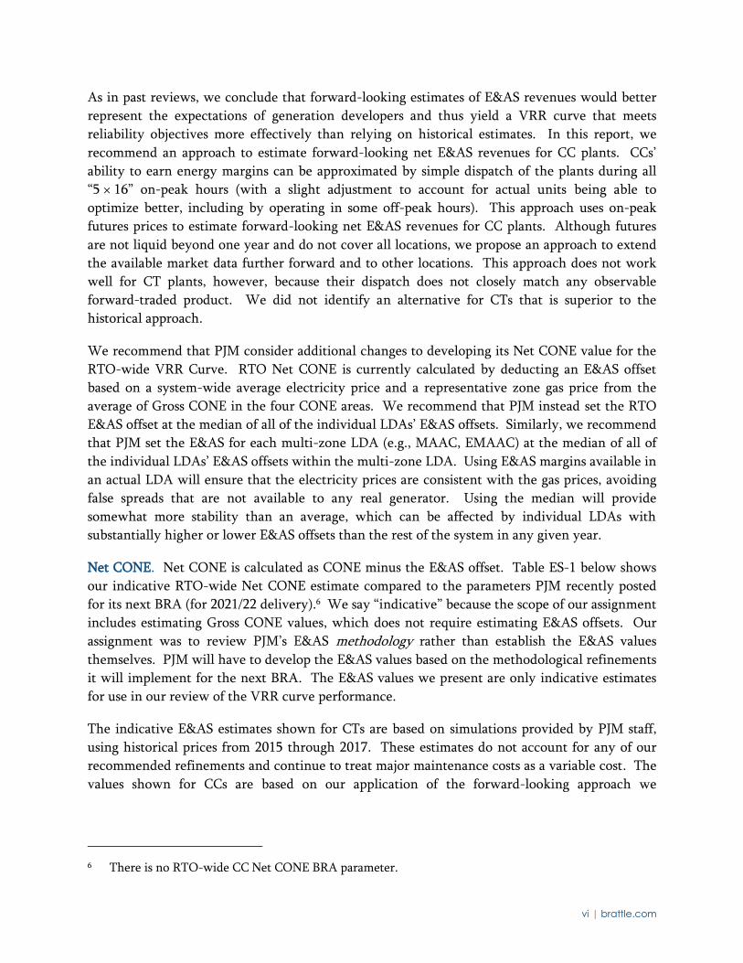
recommend for CCs; they account for the 6,300 Btu/kWh heat rate and lower variable O&M of

the new CC technology.7

Table ES-1 RTO-Wide Net CONE Estimates (Nominal Dollars)

Sources and notes:

2021/22 BRA values taken unadjusted from 2021/22 BRA parameters, PJM (2018). Brattle estimated RTO-wide E&AS are based on the median of all LDAs. Gross CONE values

reflect the average of the CONE values in each of the four CONE areas. Brattle estimates are converted from ICAP to UCAP using 2020/21 BRA EFORd rate. Major maintenance costs are included in variable O&M (VOM).

Choice of Reference Technology for VRR Curve. Our Net CONE estimate for CC plants and our

recommendation to use CCs as the reference technology is supported by empirical data showing

large quantities of CCs entering the market at prices consistent with our estimates. CCs have

been the overwhelming choice of actual new generation development over the last several years,

and nearly 27,000 MW of new combined-cycle generation has cleared PJM’s capacity auctions

since then (i.e., in auctions for delivery in 2015/16 through 2020/21). These CC plants have

entered the market at clearing prices 50-80% below PJM’s CT-based Net CONE estimates.8 As a

result, the cleared quantities in the PJM capacity auctions have exceeded the PJM reserve margin

target by 3 to 6 percentage points.9

Other considerations for selecting a reference technology include the hazard of switching

technologies used in a long-term construct, E&AS estimation error for CCs vs. CTs, year-to-year

variability in E&AS for CCs vs. CTs. We show in Section II.E that none of these factors

substantially disfavors switching to a CC.

7 The forward-looking E&AS margins based on the updated CC heat rate and variable O&M are similar

to PJM’s historical simulations using the current specifications because the lower operating costs of

the updated CC reference technology are offset by lower electricity futures prices.

8 Based on RTO clearing prices and Net CONE parameters. See Table 8, PJM (2017d). The 2017 State of

the Market report shows that market revenues in 2017 would have provided CCs with 100% of Gross

CONE in three zones and 90% in 11 zones. See Monitoring Analytics (2017). With our lower CC

Gross CONE estimates, new entrants would have covered their costs in the RTO and in 12 zones.

9 Calculated for RTO-wide cleared quantities. See PJM (2017d).

2021/22 BRA 2022/23 Brattle Estimate

CT CT CC

Gross CONE $/MW-year ICAP $135,300 $104,200 $114,400

E&AS Margin $/MW-year ICAP $24,800 $28,400 $70,600

Net CONE $/MW-year ICAP $110,500 $75,800 $43,800

Net CONE $/MW-day UCAP $322 $222 $129

viii | brattle.com

System VRR Curves

VRR curves serve as the demand curve for PJM’s capacity auctions. They are intended to

procure enough capacity to meet PJM’s resource adequacy requirements. The VRR curves are

downward-sloping and anchored to a reference point at a price given by Net CONE and a

quantity given by the installed reserve margin target, but shifted slightly rightward. Such curves

accommodate inevitable fluctuations in supply, demand, and transmission, in several ways that a

vertical capacity demand curve would not: (1) the slope recognizes that capacity has lower (but

non-zero) incremental value above the target reserve margin and higher value below; (2) the

slope reduces price volatility as market conditions fluctuate; (3) the slope mitigates potential

market power; and (4) the rightward shift adjusts for the asymmetric reliability consequences of

capacity deficits versus excesses, such that resource adequacy targets can be met on average and

years with unacceptably-low reserve margins are largely avoided. The exact slope, shape, and

shift of the curve have been developed to achieve reasonable tradeoffs between meeting resource

adequacy requirements without too much excess capacity or too much price volatility. PJM’s

periodic reviews of VRR curve performance, such as this one, re-assess these tradeoffs and

inform PJM’s updating of the VRR curve parameters and shape to maintain acceptable

performance as market conditions and technologies evolve.

To evaluate PJM’s current VRR curve and possible alternatives, we conducted Monte Carlo

simulations using an updated and enhanced version of the model that we used in the 2014

Review.10 The model evaluates capacity market outcomes probabilistically, given realistic

fluctuations in supply, demand, and transmission, and under the long-run equilibrium

assumption that merchant generation will enter the market until average prices equal Net CONE.

In this Quadrennial Review, we first updated the model to account for recent changes in system

supply, demand, transmission, LDA topology, and the effect of PJM’s new Capacity Performance

(CP) market design.11 We find that these updates have only a minor impact on simulated VRR

curve performance relative to the results from our 2014 Review, assuming the Net CONE value

used to anchor the VRR curve is equal to the actual price at which developers will enter the

market. Significant performance differences arise if that assumption does not hold.

We evaluate the performance of several candidate VRR curves accounting for the reduction in

the market entry price, as illustrated in Figure ES-1 alongside PJM’s current VRR curve from the

2021/22 auction (dark blue dashed line). Table ES-2 reports the performance results of the

candidate curves. In evaluating these candidate VRR curves, we assumed that CCs continue to

enter the market consistent with our estimate of CC Net CONE.

10 We do not re-evaluate the basic shape of the demand curve in this review. Our 2014 Review included

an extensive discussion of the basis for the shape of PJM’s VRR curve. See Pfeifenberger et al. (2014).

11 Capacity Performance has made the lower half of the capacity market supply curves more elastic,

which helps reduce price volatility and slightly improve reliability.

ix | brattle.com

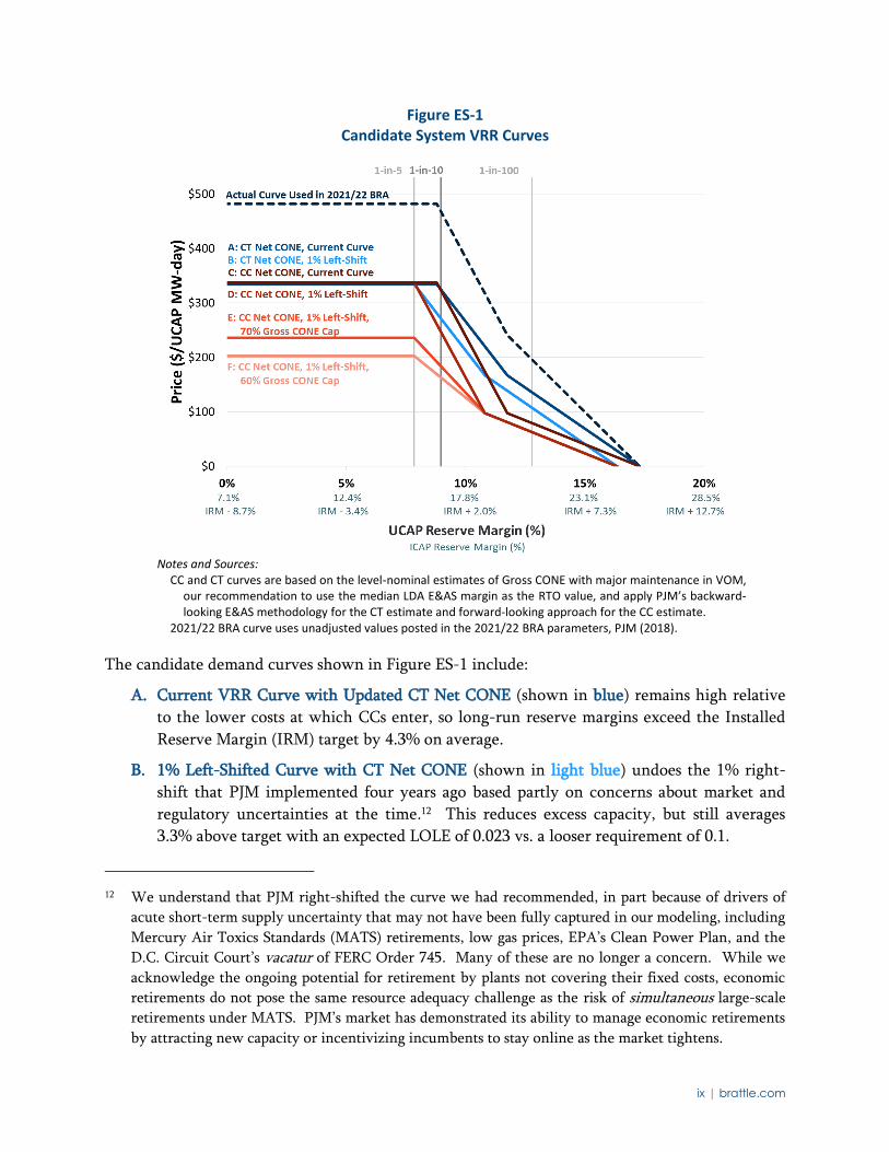
Figure ES-1 Candidate System VRR Curves

Notes and Sources:

CC and CT curves are based on the level-nominal estimates of Gross CONE with major maintenance in VOM, our recommendation to use the median LDA E&AS margin as the RTO value, and apply PJM’s backward-looking E&AS methodology for the CT estimate and forward-looking approach for the CC estimate.

2021/22 BRA curve uses unadjusted values posted in the 2021/22 BRA parameters, PJM (2018).

The candidate demand curves shown in Figure ES-1 include:

A. Current VRR Curve with Updated CT Net CONE (shown in blue) remains high relative

to the lower costs at which CCs enter, so long-run reserve margins exceed the Installed

Reserve Margin (IRM) target by 4.3% on average.

B. 1% Left-Shifted Curve with CT Net CONE (shown in light blue) undoes the 1% right-

shift that PJM implemented four years ago based partly on concerns about market and

regulatory uncertainties at the time.12 This reduces excess capacity, but still averages

3.3% above target with an expected LOLE of 0.023 vs. a looser requirement of 0.1.

12 We understand that PJM right-shifted the curve we had recommended, in part because of drivers of

acute short-term supply uncertainty that may not have been fully captured in our modeling, including

Mercury Air Toxics Standards (MATS) retirements, low gas prices, EPA’s Clean Power Plan, and the

D.C. Circuit Court’s vacatur of FERC Order 745. Many of these are no longer a concern. While we

acknowledge the ongoing potential for retirement by plants not covering their fixed costs, economic

retirements do not pose the same resource adequacy challenge as the risk of simultaneous large-scale

retirements under MATS. PJM’s market has demonstrated its ability to manage economic retirements

by attracting new capacity or incentivizing incumbents to stay online as the market tightens.

x | brattle.com

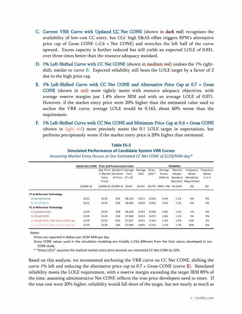
C. Current VRR Curve with Updated CC Net CONE (shown in dark red) recognizes the

availability of low-cost CC entry, but CCs’ high E&AS offset triggers RPM’s alternative

price cap of Gross CONE (=2.6 × Net CONE) and stretches the left half of the curve

upward. Excess capacity is further reduced but still yields an expected LOLE of 0.031,

over three times better than the resource adequacy standard.

D. 1% Left-Shifted Curve with CC Net CONE (shown in medium red) undoes the 1% right-

shift, similar to curve B. Expected reliability still beats the LOLE target by a factor of 2

due to the high price cap.

E. 1% Left-Shifted Curve with CC Net CONE and Alternative Price Cap at 0.7 × Gross

CONE (shown in red) more tightly meets with resource adequacy objectives, with

average reserve margins just 1.4% above IRM and with an average LOLE of 0.071.

However, if the market entry price were 20% higher than the estimated value used to

anchor the VRR curve, average LOLE would be 0.163, about 60% worse than the

requirement.

F. 1% Left-Shifted Curve with CC Net CONE and Minimum Price Cap at 0.6 × Gross CONE

(shown in light red) more precisely meets the 0.1 LOLE target in expectations, but

performs precipitously worse if the market entry price is 20% higher than estimated.

Table ES-2 Simulated Performance of Candidate System VRR Curves

Assuming Market Entry Occurs at Our Estimated CC Net CONE of $129/MW-day*

Notes:

Prices are reported in dollars per UCAP MW per day. Gross CONE values used in the simulation modeling are trivially (<1%) different from the final values developed in our

CONE study. * “Stress LOLE” assumes the realized market entry price exceeds our estimated CC Net CONE by 20%.

Based on this analysis, we recommend anchoring the VRR curve on CC Net CONE, shifting the

curve 1% left and reducing the alternative price cap to 0.7 × Gross CONE (curve E). Simulated

reliability meets the LOLE requirement, with a reserve margin exceeding the target IRM 85% of

the time, assuming administrative Net CONE reflects the true price developers need to enter. If

the true cost were 20% higher, reliability would fall short of the target, but not nearly as much as

Admin Net CONE Price and Procurement Costs Reliability

Avg. Price

(= Market

Entry

Price)

Standard

Deviation

of Price

Average

Cost

(P × Q)

Average

LOLE

Stress

LOLE *

Average

Excess

(Deficit)

Reserve

Margin

Standard

Deviation

Frequency

Below

Reliability

Requirement

Frequency

Below

1-in-5

($/MW-d) ($/MW-d) ($/MW-d) ($mil) (Ev/Yr) (Ev/Yr) (IRM + X%) (% ICAP) (%) (%)

CT as Reference Technology

A: Current Curve $222 $129 $34 $8,139 0.011 0.023 4.3% 1.1% 0% 0%

B: 1% Left-Shift $222 $129 $34 $8,065 0.023 0.041 3.3% 1.1% 0% 0%

CC as Reference Technology

C: Current Curve $129 $129 $58 $8,039 0.031 0.046 2.8% 1.1% 1% 0%

D: 1% Left-Shift $129 $129 $58 $7,969 0.053 0.072 1.8% 1.1% 5% 0%

E: 1% Left-Shift, 70% Gross CONE Cap $129 $129 $50 $7,927 0.071 0.163 1.4% 1.5% 15% 4%

F: 1% Left-Shift, 60% Gross CONE Cap $129 $129 $46 $7,906 0.091 0.331 1.1% 1.7% 20% 6%

xi | brattle.com

with the curve with the lower cap.13 Annual average procurement costs are $140 million lower

relative to the left-shifted CT-based curve (curve B), suggesting that the recommended curve

represents a reasonable tradeoff between cost and performance under adverse conditions.

Locational VRR Curves

Resource adequacy in the import-constrained LDAs depends on transmission and can be strongly

affected by fluctuations in import limits and supply that are large in percentage terms. When

reserve margins tighten and import constraints bind, the LDA capacity clearing price rises above

the parent area’s price; but when local reserve margins are high, the LDA price will fall only as

far as the clearing price in the parent zone. This asymmetric exposure helps to attract local

supply and support resource adequacy. However, LDAs with significantly higher Net CONE

than their parent areas will have to price-separate above the parent zone more frequently in

order for average clearing prices to cover the Net CONE premium, with lower reliability in those

instances.

Our analysis of VRR curves for the LDAs focuses on these dynamics, rather than the impact of

recent low market entry prices and the choice of reference technology. We simply assume that

in each location, administrative Net CONE and the market entry price are always equal to each

other, given by the 2020/21 BRA parameters. With this core assumption, we explore the impact

of potential future conditions in which LDA Net CONE values are similar to today and,

alternatively, in which they increase relative to parent zones.

For the VRR curves in LDAs, our simulations show that the updated current curve is expected to

meet resource adequacy requirements under our base assumptions—but not under potential

alternative future conditions. PJM’s locational resource adequacy standard requires that each

LDA achieves a long-run average LOLE of 1-in-25 or better (0.04 events per year).14 Under our

base assumptions with locational Net CONE values consistent with the 2020/21 BRA, most LDAs

have lower Net CONE than the parent zones. Under these conditions, LDAs easily meet the

reliability standard because costs are lower while capacity prices in LDAs cannot fall below the

prices in parent areas in PJM’s nested, import-constrained topology.

We are concerned, however, that LDA Net CONE values may not remain below those in the

parent areas in a long-run equilibrium where increased entry in the LDAs reduces E&AS offsets

and increases Net CONE there. If LDA Net CONE values were to exceed the parent LDA level, a

price premium would be needed to attract local investments. In addition, these investments

would face relatively high volatility in supply, demand, and transmission within the LDAs,

13 We also evaluated the impact of lowering the alternative price cap to 0.8 × Gross CONE, which

achieves expected LOLE of 0.061, and 0.105 in the “stress case.”

14 The 1-in-25 LOLE target for LDAs is conditional on perfect reliability in the parent zone. See PJM

(2017g), Section 2.2.

xii | brattle.com

which would increase resource adequacy challenges. If Net CONE were to become 5% higher in

each LDA compared to its parent LDA, we estimate that five of the fourteen LDAs would fail to

meet the 1-in-25 LDA standard. If Net CONE values in the LDAs were 20% above their parent

LDA levels, ten LDAs would fail to achieve the 1-in-25 LDA standard.

To address this resource adequacy risk, we evaluate two refinements to the locational VRR

curves. First, ensuring that the locational demand curves have price caps of at least 1.7 × Net

CONE would mitigate the risk of falling below LDA resource adequacy requirements by allowing

more supply to clear whenever the market is short. If PJM adopts our recommended system

curve based on CC Net CONE, with a 1% left-shift and 70% Gross CONE price cap (curve E in

Figure ES-1), the price cap would be approximately 1.8 × Net CONE. No further change would

be needed to the cap if this curve were applied at the local level. Second, establishing a

minimum demand-curve-width of 25% of the Capacity Emergency Transfer Limit (CETL) would

help mitigate the impact of CETL variability in small LDAs. This minimum curve width could be

applied to local curves of the same shape as any of the candidate system curves.

We estimate that both of these measures would individually improve resource adequacy in the

LDAs, but would still not quite achieve the 1-in-25 standard in all zones under market

conditions in which LDAs’ Net CONE values are 5% higher than in the parent areas. When the

two measures are combined, however, the 1-in-25 standard is achieved in all LDAs. We

therefore recommend that PJM consider adopting both of these measures.

In addition to our recommended changes to the LDA curves, we identified some potential

improvements to closely-related market design elements that may mitigate price volatility or

better align prices with locational reliability value. These include: (1) defining local reliability

objectives in terms of normalized unserved energy; (2) generalizing the approach to modeling

locational constraints in RPM beyond import-constrained, nested LDAs with a single import

limit; (3) reviewing options for increasing the predictability and stability of CETL estimates; and

(4) revising the auction-clearing mechanics to produce prices that are more proportional to the

marginal reliability value of incremental resources in each LDA.

13 | brattle.com

I. Background

In this study, we assess the parameters and shape of PJM Interconnection, LLC’s Variable

Resource Requirement (VRR) curve, which is used to procure capacity under the Reliability

Pricing Model (RPM). This Background section provides an overview of the structure of RPM

and the VRR curve, as well as references to more detailed documentation as available in PJM’s

Tariff and manuals.15

A. STUDY PURPOSE AND SCOPE

We have been commissioned by PJM to evaluate the parameters and shape of the administrative

VRR curve used to procure capacity under RPM, as required periodically under the PJM tariff.16

The purpose of this evaluation is to assess the effectiveness of the VRR curve in supporting the

primary RPM design objective of maintaining resource adequacy at the system and local levels, as

well as other performance objectives such as mitigating price volatility and susceptibility to the

exercise of market power. Our study scope includes: (1) estimating the Cost of New Entry for

each Locational Deliverability Area; (2) reviewing the methodology for determining the Net

Energy and Ancillary Services Revenue Offset; and (3) evaluating the shape of the VRR curve.

This report documents our analysis and findings for the second and third topic areas and

summarizes our analysis for the first. Our estimate of the Cost of New Entry is contained in a

separate report. 17

Under the first two Triennial Reviews, we assessed the overall effectiveness of RPM in

encouraging and sustaining infrastructure investments, reviewed auction results over the first

eight Base Residual Auctions (BRAs) and first seven Incremental Auctions (IAs), analyzed the

effectiveness of individual market design elements, and presented a number of recommendations

for consideration by PJM and its stakeholders. The results of these prior assessments are

presented in our June 2008 and August 2011 reports reviewing RPM’s performance (“2008 RPM

Report” and “2011 RPM Report”).

The scope of this study, like our 2014 study (“2014 RPM Report”), is more narrowly focused on

the items identified in the tariff than our 2008 and 2011 RPM Reviews. It does not include a

review and summary of RPM auction results, solicitation of stakeholder input, or an evaluation

of other RPM parameters beyond CONE, the E&AS offset, and the VRR curve.

15 As the authoritative sources documenting the structure of RPM, see Attachment DD of PJM’s Tariff,

and Manual 18, PJM (2017f, 2017h).

16 See PJM Tariff, Attachment DD.5.10.a, PJM (2017h).

17 PJM Cost of New Entry—Combustion Turbines and Combined-Cycle Plants with June 1, 2022 Online Date, prepared by The Brattle Group and Sargent & Lundy, April 2018 (“2018 CONE Study”).

14 | brattle.com

Finally, our analysis does not explicitly account for PJM’s proposed reforms to capacity market

pricing related to state policy-supported resources and the Minimum Offer Price Rule. We

assume that, with or without the proposed reforms, long-term average prices have to be high

enough to support in-market entry by gas-fired generation. Our level-nominal CONE

calculation (instead of level-real) accounts for the possibility that prices eventually decline in real

terms as other technologies enter at a lower net cost of capacity.

B. OVERVIEW OF PJM’S RELIABILITY PRICING MODEL

The purpose of RPM is to attract and retain sufficient resources to reliably meet the needs of

consumers at all locations within PJM, through a well-functioning market. It has been doing so

since its inception in 2007/08. RPM is now entering its fifteenth delivery year of experience,

with the next auction scheduled for May 2018 to procure capacity for the 2021/22 delivery year.

RPM is a centralized market for procuring capacity on behalf of all load, with all capacity

procured through BRAs conducted three years prior to delivery and adjustments to load forecasts

and supply settled through shorter-term IAs. The costs of these capacity procurements are

allocated to load serving entities (LSEs) throughout the actual delivery year. “Demand” in PJM’s

auctions is described by the VRR curve, a segmented, downward-sloping, convex curve that is

designed to procure enough capacity to meet resource adequacy objectives while avoiding the

extreme price volatility that a vertical curve might produce. Recognizing transmission

constraints, each of several nested LDAs has its own VRR curve that may set higher prices locally

if transmission constraints bind in the auction.

On the supply side, a diverse set of existing and new resources compete to sell capacity under

RPM, including traditional and renewable generation, demand response, energy efficiency,

storage, qualified transmission projects, and imports. Existing resources are required to submit

an offer, subject to market monitoring and mitigation. Some types of new resources are also

monitored to ensure they are being introduced at competitive levels that do not artificially

suppress prices. With the introduction of Capacity Performance, all capacity sellers must be

available across the full delivery year. Resources available only in one season may still

participate by pairing up with an opposite-season resource ahead of the auction, or by allowing

PJM’s auction clearing mechanism to find a suitable match. Capacity Performance has

considerably strengthened penalties charged to non-performing resources and has introduced

bonuses for resources that perform better than expected.

RPM allows for self-supply arrangements, whereby entities with load-serving obligations can sell

supply into the auction and earn revenues that offset the load’s payments on the demand side.

RPM has an opt-out mechanism in which self-supply utilities can meet a Fixed Resource

Requirement (FRR) instead of a variable requirement.

15 | brattle.com

Attachment DD of PJM’s Open Access Transmission Tariff (OATT) and PJM’s Manual 18

describe in greater detail these and other features of the RPM market design.18 Additional

documentation on the parameters and performance of PJM’s RPM include: (a) PJM’s planning

period parameters and auction results; (b) our 2008, 2011, and 2014 RPM performance Reviews;

and (c) performance assessments of PJM’s Independent Market Monitor (IMM), as documented

in annual State of the Market Reports, assessments of individual auctions’ results, and other

issue-specific reports.19

C. DESCRIPTION OF THE VARIABLE RESOURCE REQUIREMENT CURVE

In our 2014 RPM Review, we recommended that PJM adopt a downward-sloping, convex VRR

curve, set to achieve 0.1 LOLE on average in the long run. At lower reserve margins, additional

supply brings substantial improvement in reliability due to the steepness of the LOLE curve in

this region, as shown in Figure 16. At higher reserve margins, additional supply brings relatively

less improvement. The convex shape quickly pays more for supply when the market is short and

more gradually reduces prices as the market becomes long, aligning prices with the reliability

value of incremental supply. In addition, the convex curve tends to produce a distribution of

market prices that is more consistent with those of other commodity markets, with a fatter tail

on the high-price side. Perhaps most importantly, a convex curve is more robust from a quantity

perspective, with changes to Net CONE or errors in Net CONE producing smaller reliability

deviations from the resource adequacy target than straight-line or concave curves.

Following our 2014 Review, PJM proposed, and the Federal Energy Regulatory Commission

(FERC) accepted, a convex VRR curve that was right-shifted by 1% relative to our recommended

curve. PJM pointed out that while our recommended curve achieved 0.1 LOLE on average, it

frequently resulted in low reliability outcomes below the 1-in-5 LOLE level (13% of the time)

and did not perform well under adverse conditions (e.g., larger than expected fluctuations in net

supply, administrative under-estimation of Net CONE). PJM’s right-shifted convex VRR curve

reduced the likelihood of outcomes below the 1-in-5 level to 7% and performed well under

adverse conditions, while only increasing customer costs by 1% in our simulations.20

The prices and quantities of the VRR curve are premised on the assumption that, in a long-term

economic equilibrium, prices need to be at Net CONE on average to attract new entrants when

needed for reliability. Net CONE is the first-year capacity revenue a new generation resource

would need (in combination with expected E&AS margins) to fully recover its capital and fixed

costs, given reasonable expectations about future cost recovery over the asset life. The price at

each point on the VRR curve is indexed to Net CONE. The price cap is well above Net CONE

18 See PJM (2017f, 2017h).

19 See PJM Planning Period Parameters for the years 2007–2017, Pfeifenberger (2008, 2011, 2014). For

PJM State of the Market and periodic reports on RPM, see Monitoring Analytics (2014, 2017).

20 See PJM (2014f).

16 | brattle.com

(1.5 × on PJM’s current VRR curve), the kink is somewhat below Net CONE (0.75 × on PJM’s

current VRR curve), and the foot is at a price of zero. In order to account for variability and to

achieve the resource adequacy requirement (quantity needed to meet the 1 event in 10 years, or

1-in-10, LOLE standard) on average, the VRR curve quantity is greater than the desired average

reserve margin at a price of Net CONE. Prices decline as reserve margins increase and rise as

reserve margins decrease, but all price points on the curve are indexed to Net CONE.

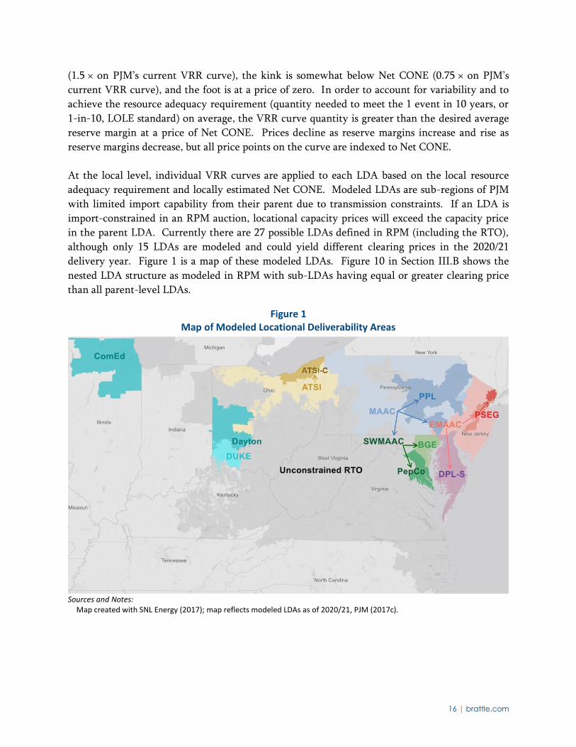
At the local level, individual VRR curves are applied to each LDA based on the local resource

adequacy requirement and locally estimated Net CONE. Modeled LDAs are sub-regions of PJM

with limited import capability from their parent due to transmission constraints. If an LDA is

import-constrained in an RPM auction, locational capacity prices will exceed the capacity price

in the parent LDA. Currently there are 27 possible LDAs defined in RPM (including the RTO),

although only 15 LDAs are modeled and could yield different clearing prices in the 2020/21

delivery year. Figure 1 is a map of these modeled LDAs. Figure 10 in Section III.B shows the

nested LDA structure as modeled in RPM with sub-LDAs having equal or greater clearing price

than all parent-level LDAs.

Figure 1 Map of Modeled Locational Deliverability Areas

Sources and Notes:

Map created with SNL Energy (2017); map reflects modeled LDAs as of 2020/21, PJM (2017c).

17 | brattle.com

II. Net Cost of New Entry Parameter

Net CONE is determined as the estimated annualized fixed costs of new entry, or Gross CONE, of

the reference resource, net of estimated E&AS margins and expected performance bonus. We

examine PJM’s current conditions and recent new installed capacity and conclude the following:

Net CONE for a gas-fired combustion turbine (CT)—the current reference technology for

the VRR curve as specified in PJM’s tariff—is now 25-42% lower than PJM’s 2021/22 Net

CONE parameter, depending on location.21 The decline is primarily driven by the

economies of scale of new H-class CTs, the lower corporate tax rate and, to a lesser

extent, a slightly lower cost of capital.

Net CONE for gas-fired combined-cycles (CCs)—the dominant technology of new

generation in PJM for more than fifteen years— is 44-76% lower than PJM’s 2021/22 CT-

based Net CONE parameter, and 25-63% below the updated CT Net CONE estimate,

depending on location. This difference is mostly due to the much higher E&AS revenues

of CCs and plant costs that are only slightly higher than those of CTs on a dollar-per-kW

basis.

Based on the economic advantage of CCs over CTs and the prevalence of CCs in new

generation investments in the PJM market, we recommend that PJM consider adopting

the CC as the reference technology for anchoring the VRR curve.

We also propose relatively minor changes to the way historical E&AS offsets are

calculated for CTs, a method for estimating forward-looking E&AS offsets for a CC based

on on-peak futures settlement prices, and a different averaging technique for calculating

the RTO-wide value for Net CONE.

A. UPDATED GROSS CONE ESTIMATES

The administrative Gross CONE value reflects the total annual net revenues a new generation

resource needs to earn on average to recover its capital investment and annual fixed costs, given

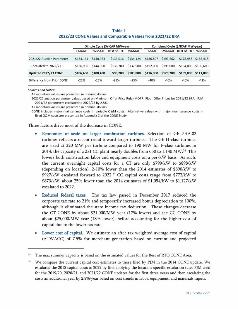
reasonable expectations about future cost recovery over its economic life. Table 1 summarize our

CONE estimates for gas CT and CC plants in each of the four PJM CONE Areas for the 2022/23

delivery year.22 Detailed documentation of these CONE estimates and our study approach is

provided in our separate CONE study.23

21 The differences across zones are largely due to differences in the net E&AS revenue offset.

22 Previous CONE studies had five CONE Areas, but the Dominion CONE Area was removed in recent

tariff changes and is now included in the Rest of RTO CONE Area.

23 See Newell et al. (2018).

18 | brattle.com

Table 1 2022/23 CONE Values and Comparable Values from 2021/22 BRA

Sources and Notes:

All monetary values are presented in nominal dollars. 2021/22 auction parameter values based on Minimum Offer Price Rule (MOPR) Floor Offer Prices for 2021/22 BRA. PJM

2021/22 parameters escalated to 2022/23 by 2.8%. All monetary values are presented in nominal dollars. CONE includes major maintenance costs in variable O&M costs. Alternative values with major maintenance costs in

fixed O&M costs are presented in Appendix C of the CONE Study.

Three factors drive most of the decrease in CONE:

Economies of scale on larger combustion turbines. Selection of GE 7HA.02

turbines reflects a recent trend toward larger turbines. The GE H-class turbines

are sized at 320 MW per turbine compared to 190 MW for F-class turbines in

2014; the capacity of a 2x1 CC plant nearly doubles from 650 to 1,140 MW.24 This

lowers both construction labor and equipment costs on a per-kW basis. As such,

the current overnight capital costs for a CT are only $799/kW to $898/kW

(depending on location), 2-10% lower than the 2014 estimates of $890/kW to

$927/kW escalated forward to 2022.25 CC capital costs range from $772/kW to

$873/kW, about 25% lower than the 2014 estimates of $1,054/kW to $1,127/kW

escalated to 2022.

Reduced federal taxes. The tax law passed in December 2017 reduced the

corporate tax rate to 21% and temporarily increased bonus depreciation to 100%,

although it eliminated the state income tax deduction. These changes decrease

the CT CONE by about $21,000/MW-year (17% lower) and the CC CONE by

about $25,000/MW-year (18% lower), before accounting for the higher cost of

capital due to the lower tax rate.

Lower cost of capital. We estimate an after-tax weighted-average cost of capital

(ATWACC) of 7.5% for merchant generation based on current and projected

24 The max summer capacity is based on the estimated values for the Rest of RTO CONE Area.

25 We compare the current capital cost estimates to those filed by PJM in the 2014 CONE update. We

escalated the 2018 capital costs to 2022 by first applying the location-specific escalation rates PJM used

for the 2019/20, 2020/21, and 2021/22 CONE updates for the first three years and then escalating the

costs an additional year by 2.8%/year based on cost trends in labor, equipment, and materials inputs.

Simple Cycle ($/ICAP MW-year) Combined Cycle ($/ICAP MW-year)

EMAAC SWMAAC Rest of RTO WMAAC EMAAC SWMAAC Rest of RTO WMAAC

2021/22 Auction Parameter $133,144 $140,953 $133,016 $134,124 $186,807 $193,562 $178,958 $185,418

...Escalated to 2022/23 $136,900 $144,900 $136,700 $137,900 $192,000 $199,000 $184,000 $190,600

Updated 2022/23 CONE $106,400 $108,400 $98,200 $103,800 $116,000 $120,200 $109,800 $111,800

Difference from Prior CONE -22% -25% -28% -25% -40% -40% -40% -41%

19 | brattle.com

capital market conditions and the change in the corporate tax rate (which varies

slightly across locations due to differences in state tax rates). Compared to an

ATWACC of 8.0% in the 2014 study, the lower ATWACC reduces the annual

CONE value by 3.7% for CTs and 3.8% CCs.

We present in this report and the CONE study two versions of the updated 2022/23 CONE values

due to the uncertainty as to whether major maintenance costs will be allowed to be included in

variable O&M costs, pending an ongoing stakeholder process.26 This report focuses on the CONE

and E&AS values with these costs in the variable O&M for comparability to prior studies and

parameter values (and the possibility that PJM will change its Cost Development Guidelines back

to be consistent with those). Classifying these costs as fixed instead of variable increases CONE

by $19,000/MW-year for CTs (a 19% increase) and $10,000/MW-year for CCs (a 9% increase).

Removing these costs from variable O&M will increase Net E&AS revenues and offset some (or

all) of the increased CONE value in the calculation of Net CONE.

B. NET E&AS REVENUE OFFSET

PJM calculates the Net CONE by subtracting the net energy and ancillary service (E&AS)

revenues from the Gross CONE; net E&AS revenues are calculated using historical prices and the

Peak-Hour Dispatch method, as defined in PJM’s tariff (the calculation for CCs uses a modified

version of the Peak-Hour Dispatch).27 We assessed whether this E&AS methodology provides a

reasonable estimate of the net E&AS revenues developers expect when constructing their

reservation prices for participating in PJM’s Base Residual Auctions.

Our conclusions are that the tariff-mandated Peak-Hour Dispatch method for estimating CCs’

historical net E&AS revenues is validated by comparison to the actual net revenues earned by

representative units.28 For CTs, there are too few representative existing resources to make a

meaningful comparison, but PJM’s approach and assumptions are reasonable. However, we have

identified several refinements to more accurately reflect the variable costs and revenues of the

reference units: adopting the updated reference resource characteristics (i.e., heat rate, capacity,

variable O&M costs) estimated in the concurrently-released 2018 CONE Study; and changing the

representative gas hubs for six transmission zones.

PJM can further improve its Net E&AS estimates for CCs by adopting a forward-looking

approach that accounts for expected changes in market conditions and reduces the volatility of

26 See: http://www.pjm.com/committees-and-groups/committees/mic.aspx

27 See PJM Tariff, Attachment DD.5.10(a)(v), PJM (2017h) for a description of PJM’s Peak-Hour

Dispatch method for a CT. For the CC, we use a modified version of the peak-hour dispatch as

described in DD.5.14(h)(3)(ii).

28 The IMM provided the net energy revenues for representative plants based on its estimate of total

energy and make-whole revenues minus fuel, variable operations and maintenance, and other costs.

http://www.pjm.com/committees-and-groups/committees/mic.aspx

20 | brattle.com

historical simulations. Our analysis shows that CC energy margins can be closely approximated

by assuming a simple dispatch against futures prices. This approach would allow PJM to use the

observable market-based futures prices that developers rely on for their own forecasts to set the

Net E&AS revenue offset. While futures are not liquid three years forward and do not cover all

of the locations in PJM, we identified market data that PJM can use as proxies for extending the

price forward and to all of the PJM transmission zones. We considered a similar approach for

CTs, but have not identified any good proxies that are comparable to CCs using futures prices.

1. PJM’s Peak-Hour Dispatch Against Historical Prices

We attempted to assess the accuracy of PJM’s approach by comparing PJM’s historical simulation

results to actual historical revenues of representative plants that are similar to the reference

resources. For CCs, there are numerous representative plants with comparable heat rate and unit

size. For CTs, we did not identify any representative existing plants because there are limited

recent new CTs and most of the existing CTs are not equipped with selective catalytic reduction

(SCRs), and so must accept strict federally-enforced run limits within their Title IV air permits.

These run limits inhibit the ability of the CTs from operating as often as the reference CT

specified in the CONE study, especially during recent periods of low gas prices.

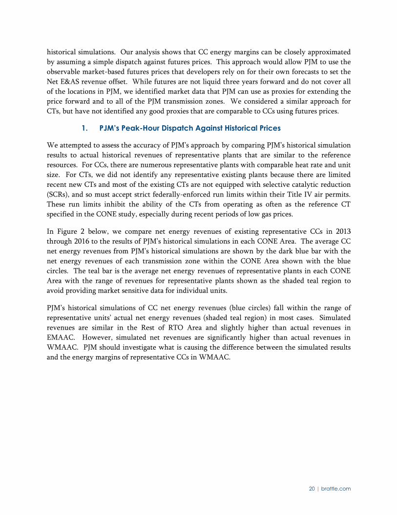
In Figure 2 below, we compare net energy revenues of existing representative CCs in 2013

through 2016 to the results of PJM’s historical simulations in each CONE Area. The average CC

net energy revenues from PJM’s historical simulations are shown by the dark blue bar with the

net energy revenues of each transmission zone within the CONE Area shown with the blue

circles. The teal bar is the average net energy revenues of representative plants in each CONE

Area with the range of revenues for representative plants shown as the shaded teal region to

avoid providing market sensitive data for individual units.

PJM’s historical simulations of CC net energy revenues (blue circles) fall within the range of

representative units’ actual net energy revenues (shaded teal region) in most cases. Simulated

revenues are similar in the Rest of RTO Area and slightly higher than actual revenues in

EMAAC. However, simulated net revenues are significantly higher than actual revenues in

WMAAC. PJM should investigate what is causing the difference between the simulated results

and the energy margins of representative CCs in WMAAC.

21 | brattle.com

Figure 2 CC Net Energy Revenues

Sources and Notes:

Historical simulations provided by PJM. Representative unit net revenues provided by IMM. There were no representative CC units in SWMAAC during this time period and too few

representative CC units in WMAAC to avoid releasing market-sensitive information.

Although the historical CC estimates are reasonably consistent with representative units, we

recommend that PJM consider the following changes to its simulations to accurately capture

future net energy revenues and that PJM add an estimate of payments a new unit can expect

under the Capacity Performance market design.

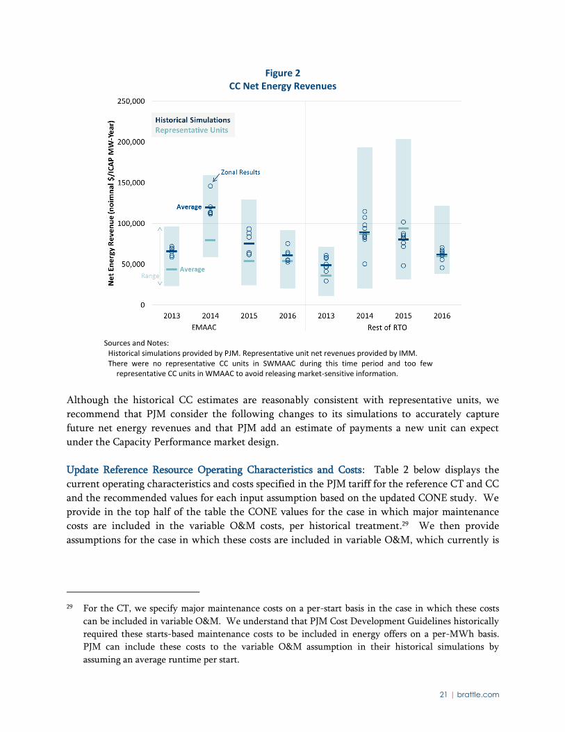
Update Reference Resource Operating Characteristics and Costs: Table 2 below displays the

current operating characteristics and costs specified in the PJM tariff for the reference CT and CC

and the recommended values for each input assumption based on the updated CONE study. We

provide in the top half of the table the CONE values for the case in which major maintenance

costs are included in the variable O&M costs, per historical treatment.29 We then provide

assumptions for the case in which these costs are included in variable O&M, which currently is

29 For the CT, we specify major maintenance costs on a per-start basis in the case in which these costs

can be included in variable O&M. We understand that PJM Cost Development Guidelines historically

required these starts-based maintenance costs to be included in energy offers on a per-MWh basis.

PJM can include these costs to the variable O&M assumption in their historical simulations by

assuming an average runtime per start.

22 | brattle.com

not allowed for cost-based energy offers but may change as the result of an ongoing stakeholder

process.30

The updated heat rates reflect the more efficient H-class turbines recommended in the CONE

study and will increase net energy revenues in PJM’s historical simulations. The recommended

variable O&M costs for both cases are significantly lower than the current assumptions that were

specified in the Tariff in 2008. Over the past ten years, variable O&M costs have declined due to

the economies of scale of the larger turbines and the increased duration between maintenance

intervals recommended by the manufacturers. The lower variable O&M costs will also increase

net energy revenues.31

Table 2 Historical Simulation Reference Resource Assumptions

(under two alternative treatments of major maintenance costs)

Source and notes:

Current values specified in PJM Interconnection, L.L.C. (2015), Open Access Transmission Tariff, effective date 4/1/2015, accessed 2/7/2018, Section 5.10 a., 5.14 h.

Net Heat Rate is estimated at ISO conditions of 59°F, 60% Relative Humidity, and at mean sea level consistent with the value in the tariff.

CT Updated Total Variable O&M of $7.00/MWh includes $5.90/MWh of major maintenance costs assuming $23,464/start from the CONE study, 11.1 hours per start (based on results of the tariff-mandated simulation), and average capacity of 358 MW across CONE Areas.

Update Natural Gas Price Hubs: The increase in natural gas production in the Marcellus

formation since 2014 has shifted gas flows across the PJM region and altered pricing dynamics in

30 There is an ongoing process underway in the Markets Implementation Committee concerning the cost

guidelines for CTs and CCs. Currently, these costs are not allowed to be included in cost-based energy

offers. If the guidelines do allow the costs to be included in the future, PJM should analyze whether

suppliers include these costs in their price-based offers or not. If PJM determines that their offers do

include these costs then PJM should adopt the costs and associated CONE values with major

maintenance and overhaul costs in the variable O&M.

31 We also recommend updates to the startup cost assumptions for the updated reference resources in

PJM’s historical simulations, which are included in Appendix B of the CONE study.

CT CC

Current Updated Current Updated

Major Maintenance in Variable O&M, per historical treatment

Net Heat Rate Btu/kWh, HHV 10,096 9,134 6,722 6,269

Net Heat Rate with Duct Firing Btu/kWh, HHV - - - 6,501

Total Variable O&M $/MWh $6.47 $7.00 $3.23 $2.11

Major Maintenance in Fixed O&M and CONE, consistent with PJM's current cost guidelines

Total Variable O&M $/MWh $6.47 $1.10 $3.23 $0.67

23 | brattle.com

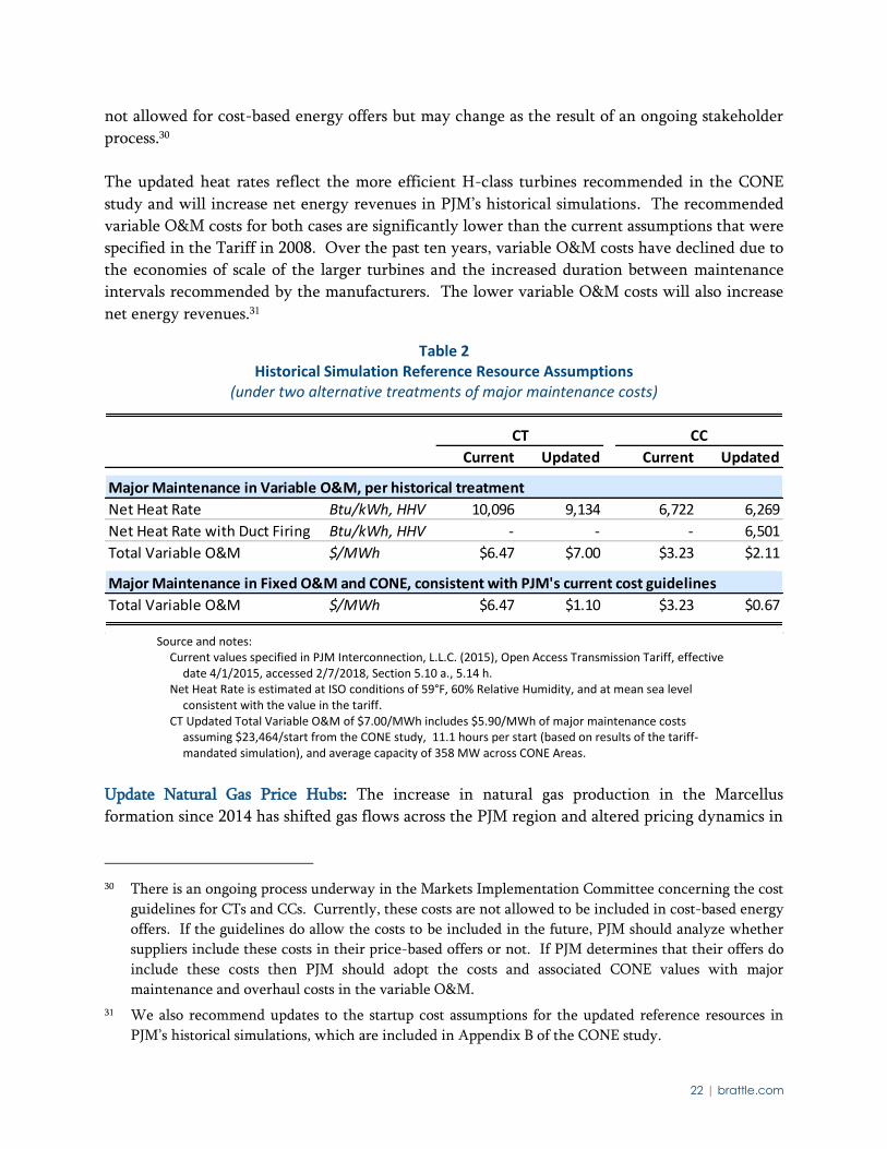
ways that were not present when PJM last updated the representative gas hubs. We reviewed

the assumed hubs used in the historical simulation for setting the gas prices in each zone and

recommend that PJM consider updating the reference gas hub for six zones, as shown in Table 3.

In reviewing the relevant gas hubs for each zone, we preferred to rely on gas hubs with greater

trading volumes (e.g., Transco Leidy Line instead of Dominion North for PENELEC), considered

constraints on the Columbia Appalachia system that have led to price disparity between

Columbia Gas Appalachia TCO Pool and other Appalachian pricing hubs (e.g., Dominion South

instead of Columbia-App/TCO Pool for APS), and reviewed the reference gas hubs used by Platts

and Energy Velocity for each zone (e.g., Transco-Zone 5 Delivered instead of Transco Zone 6

non-NY for PEPCO). In addition, PJM should consider calculating the gas price for PSEG as an

average of the Transco Zone 6 NY and Non-NY prices to provide a representative gas price for

the entire zone, which stretches from northern New Jersey (where the Transco Zn 6 NY price is

more relevant) to southern New Jersey (where the non-NY price is more relevant).

We also reviewed the gas transportation adders that PJM uses to calculate delivered gas prices,

which range from $0.00 to $0.10/MMBtu in most zones and $0.15 to $0.20/MMBtu in COMED.

Due to the access to interstate pipelines throughout the PJM footprint and the assumed cost of a

gas lateral in the CONE study, we recommend that PJM consider eliminating the use of all

transportation adders.

Table 3 Recommended Changes to Historical Simulation Representative Gas Hubs

Sources and Notes:

The recommendation for PSEG is a 50%-50% blend of Transco-Z6 (NY) and Transco-Z6 (non-NY) prices. EV data downloaded from ABB Inc.’s Energy Velocity Suite and Platts data downloaded from S&P Global Market Intelligence

between August and December 2017.

Consider Including a Gas Balancing Cost Adder for CTs: PJM commits and dispatches CTs

during the operating day just a few hours before delivery, forcing them to arrange gas deliveries

or to balance pre-arranged gas deliveries on the operating day. Generators may thus incur

balancing penalties or have to buy or sell gas in illiquid intra-day markets. This may increase the

average cost of procuring gas above the price implied by day-ahead hub prices. However, these

costs are not transparent and may not follow regular patterns that are easily amenable to analysis.

Our interviews with generation companies provided mixed reactions. Some with larger fleets

claimed that they can manage their gas across their fleets without paying any more on average

Current PJM BrattleZone Reference Gas Hubs Recommendations Reason for Change

APS Columbia-APP/TCO Pool Dominion South Constraints on the Columbia Appalachia System

DUQ Columbia-APP/TCO Pool Dominion South Constraints on the Columbia Appalachia System

PENELEC Dominion-NORTH Transco Leidy Line Limited liquidity of Dominion North

PEPCO Transco-Z6 (non-NY) Transco-Z5 Dlv Relevant hub identified by Platts and EV

PPL TETCO M3 Transco Leidy Line Relevant hub identified by Platts and EV

PSEG Transco-Z6 (NY) Blend (see notes) Zone-wide representative price

24 | brattle.com

than the prices implied by the day-ahead hub prices. Others suggested that they might incur

extra costs of up $0.30/MMBtu. We recommend that PJM investigate this further and consider

applying the 10% cost offer adder allowed under PJM’s Operating Agreement to the variable

operating costs of the CTs in the simulations.32

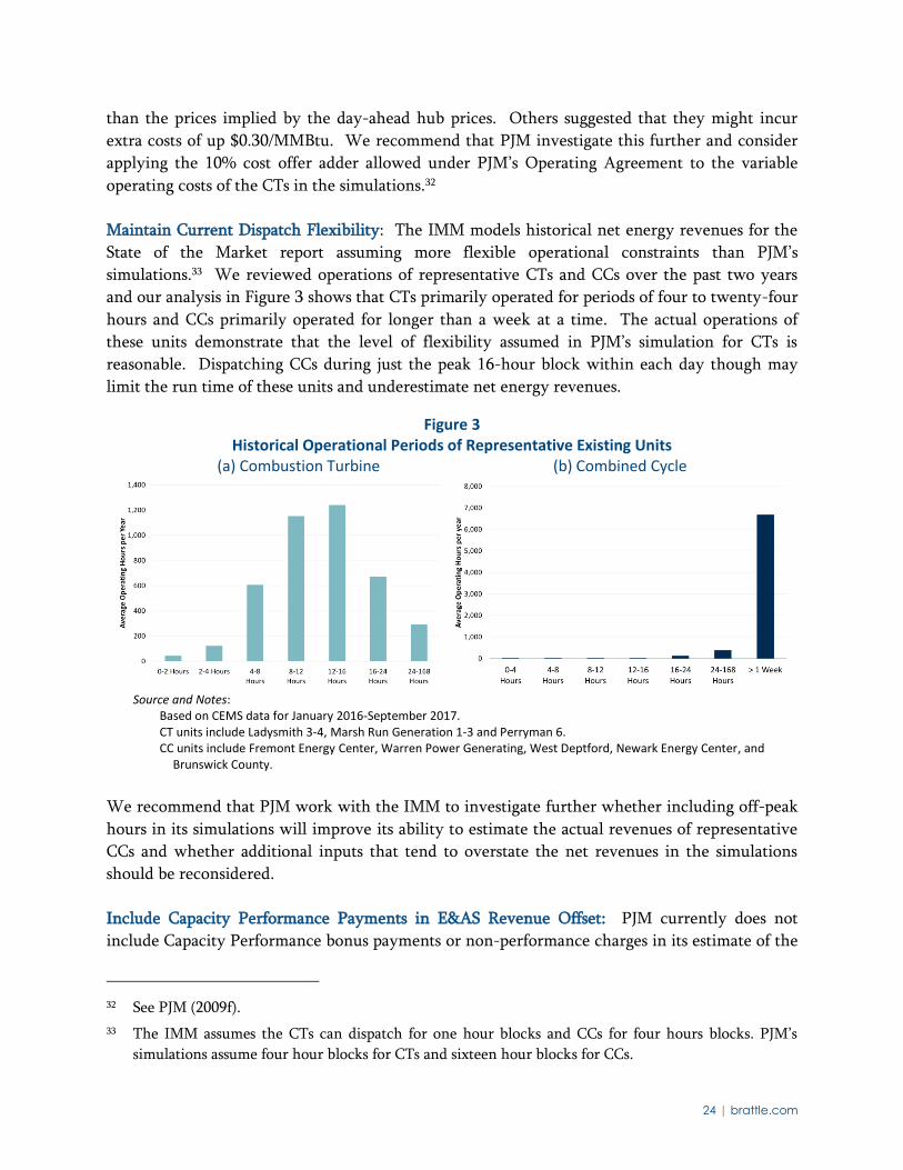
Maintain Current Dispatch Flexibility: The IMM models historical net energy revenues for the

State of the Market report assuming more flexible operational constraints than PJM’s

simulations.33 We reviewed operations of representative CTs and CCs over the past two years

and our analysis in Figure 3 shows that CTs primarily operated for periods of four to twenty-four

hours and CCs primarily operated for longer than a week at a time. The actual operations of

these units demonstrate that the level of flexibility assumed in PJM’s simulation for CTs is

reasonable. Dispatching CCs during just the peak 16-hour block within each day though may

limit the run time of these units and underestimate net energy revenues.

Figure 3 Historical Operational Periods of Representative Existing Units

(a) Combustion Turbine (b) Combined Cycle

Source and Notes:

Based on CEMS data for January 2016-September 2017. CT units include Ladysmith 3-4, Marsh Run Generation 1-3 and Perryman 6. CC units include Fremont Energy Center, Warren Power Generating, West Deptford, Newark Energy Center, and

Brunswick County.

We recommend that PJM work with the IMM to investigate further whether including off-peak

hours in its simulations will improve its ability to estimate the actual revenues of representative

CCs and whether additional inputs that tend to overstate the net revenues in the simulations

should be reconsidered.

Include Capacity Performance Payments in E&AS Revenue Offset: PJM currently does not

include Capacity Performance bonus payments or non-performance charges in its estimate of the

32 See PJM (2009f).

33 The IMM assumes the CTs can dispatch for one hour blocks and CCs for four hours blocks. PJM’s

simulations assume four hour blocks for CTs and sixteen hour blocks for CCs.

25 | brattle.com

E&AS revenue offset. Based on the approximately 10 scarcity performance hours implied in

recent BRA offers,34 our analysis shows that a new CT and CC would receive on average about

$2,000/MW-year in net performance payments.35 We recommend that PJM include an estimate

of the performance payments (or potential charges) when setting future Net E&AS revenue

offsets. PJM could calculate the performance payments based on recent historical payments to

representative units, similar to the energy margins, or use an approach similar to the calculation

above if PJM’s adopts a forward-looking estimate of energy margins.

2. Option for a Forward-Looking E&AS Offset Approach

PJM should consider estimating the Net E&AS revenue offset using a forward-looking approach

that will provide a better representation of developer’s expectations for net energy revenues. We

recommend that PJM adopt a forward-looking approach for CCs because CC net energy revenues

can be reasonably approximated during on-peak hours. This allows the use of observable futures

prices to estimate net energy revenues. While the futures at the most-heavily traded hub in PJM,

Western Hub, are not liquid beyond a year or two forward, we developed an approach that

utilizes the best available market data to project future net E&AS revenues. However, this

approach does not work well for CTs, because their dispatch does not closely match any

observable forward-traded product. We did not identify an alternative for CTs that is superior to

the historical approach.

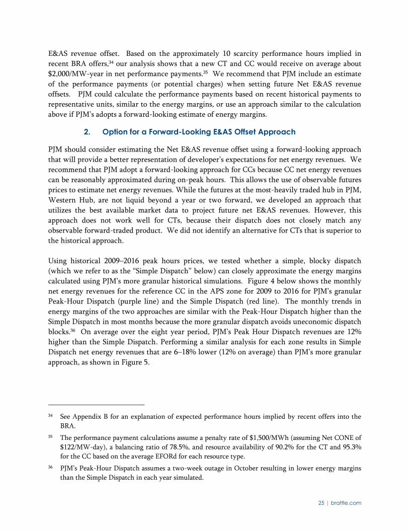
Using historical 2009–2016 peak hours prices, we tested whether a simple, blocky dispatch

(which we refer to as the “Simple Dispatch” below) can closely approximate the energy margins

calculated using PJM’s more granular historical simulations. Figure 4 below shows the monthly

net energy revenues for the reference CC in the APS zone for 2009 to 2016 for PJM’s granular

Peak-Hour Dispatch (purple line) and the Simple Dispatch (red line). The monthly trends in

energy margins of the two approaches are similar with the Peak-Hour Dispatch higher than the

Simple Dispatch in most months because the more granular dispatch avoids uneconomic dispatch

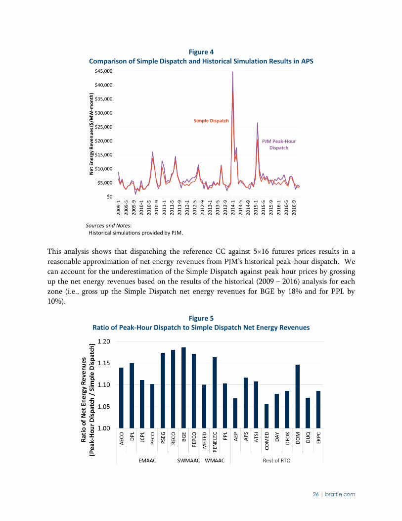
blocks.36 On average over the eight year period, PJM’s Peak Hour Dispatch revenues are 12%

higher than the Simple Dispatch. Performing a similar analysis for each zone results in Simple

Dispatch net energy revenues that are 6–18% lower (12% on average) than PJM’s more granular

approach, as shown in Figure 5.

34 See Appendix B for an explanation of expected performance hours implied by recent offers into the

BRA.

35 The performance payment calculations assume a penalty rate of $1,500/MWh (assuming Net CONE of

$122/MW-day), a balancing ratio of 78.5%, and resource availability of 90.2% for the CT and 95.3%

for the CC based on the average EFORd for each resource type.

36 PJM’s Peak-Hour Dispatch assumes a two-week outage in October resulting in lower energy margins

than the Simple Dispatch in each year simulated.

26 | brattle.com

Figure 4 Comparison of Simple Dispatch and Historical Simulation Results in APS

Sources and Notes:

Historical simulations provided by PJM.

This analysis shows that dispatching the reference CC against 5×16 futures prices results in a

reasonable approximation of net energy revenues from PJM’s historical peak-hour dispatch. We

can account for the underestimation of the Simple Dispatch against peak hour prices by grossing

up the net energy revenues based on the results of the historical (2009 – 2016) analysis for each

zone (i.e., gross up the Simple Dispatch net energy revenues for BGE by 18% and for PPL by

10%).

Figure 5 Ratio of Peak-Hour Dispatch to Simple Dispatch Net Energy Revenues

27 | brattle.com

The PJM Western Hub electricity futures are the most liquid in PJM, but there is limited trading

volume on contracts three years forward and do not reflect prices across the PJM market.37

However, our analysis shows that the reported 2021/22 Western Hub on-peak prices reflect the

trends in gas prices and near-term market heat rates. (Note that we estimate 2021/22 electricity

prices and CC E&AS margins using the forward-looking approach to compare to the 2015-2017

historical simulations used for the upcoming 2021/22 BRA.) For this reason, we find that they

are a significant improvement to using historical gas and electricity prices for estimating the net

energy revenues for new CCs three-years forward.38 The 2021/22 Western Hub on-peak prices

can also be extended to each of the PJM transmission zones by using the most recent long-term

Financial Transmission Rights (FTR) auction results.39 We developed zone-specific on-peak

electricity prices by starting with the Western Hub futures prices and applying the annual

congestion between Western Hub and each transmission zone implied by the long-term on-peak

FTR auction results. The monthly electricity prices can then be shaped based on the historical

average electricity prices in each zone and adjusted for historical differences in losses between

Western Hub and each zone.

Figure 6 shows the projected monthly electricity prices for one zone in each CONE Area through

the 2021/22 commitment period. The projected prices continue to peak in the winter, especially

in the MAAC Areas, and trend slightly downward with 2021/22 prices on average about 7%

lower than 2015-17 peak prices. Prices decline more significantly in MAAC than Rest of RTO

due to differences in congestion implied by long-term FTRs; BGE prices are 16% lower than

recent historical prices, while COMED prices (not shown) are just 2.5% lower.

37 The Open Interest on PJM Western Hub futures contracts steadily declines from nearly 6,000 per

month over the next year to zero in 2022.

38 We developed a fundamentals-based projection of Western Hub prices using the best available market

data: the long-term Henry Hub gas futures (which have open interest out to 2022); the near-term basis

differentials between Henry Hub and Dominion South futures (the gas hub with the most liquidity in

PJM’s footprint); and, the near-term market heat rates implied by Dominion South and Western Hub.

We used these components to project Western Hub prices in 2021/22 by starting with the long-term

Henry Hub gas prices, adding the near-term monthly Dominion South basis differentials (assuming

basis differentials remain constant in real dollars), and finally multiplying the resulting gas prices by

the near-term monthly market heat rates. The projected Western Hub prices closely align with the

current long-term Western Hub prices.

39 The long-term FTR auctions conducted in 2017 included FTRs out to 2020/21. For projecting the

values forward to 2021/22, we assume FTRs will scale with Western Hub prices. PJM posts FTR

auction results here: http://www.pjm.com/markets-and-operations/ftr.aspx

http://www.pjm.com/markets-and-operations/ftr.aspx

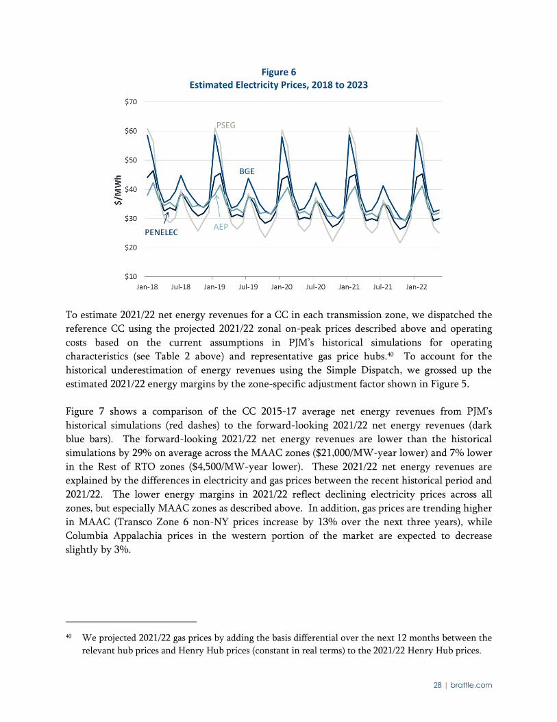
28 | brattle.com

Figure 6 Estimated Electricity Prices, 2018 to 2023

To estimate 2021/22 net energy revenues for a CC in each transmission zone, we dispatched the

reference CC using the projected 2021/22 zonal on-peak prices described above and operating

costs based on the current assumptions in PJM’s historical simulations for operating

characteristics (see Table 2 above) and representative gas price hubs.40 To account for the

historical underestimation of energy revenues using the Simple Dispatch, we grossed up the

estimated 2021/22 energy margins by the zone-specific adjustment factor shown in Figure 5.

Figure 7 shows a comparison of the CC 2015-17 average net energy revenues from PJM’s

historical simulations (red dashes) to the forward-looking 2021/22 net energy revenues (dark

blue bars). The forward-looking 2021/22 net energy revenues are lower than the historical

simulations by 29% on average across the MAAC zones ($21,000/MW-year lower) and 7% lower

in the Rest of RTO zones ($4,500/MW-year lower). These 2021/22 net energy revenues are

explained by the differences in electricity and gas prices between the recent historical period and

2021/22. The lower energy margins in 2021/22 reflect declining electricity prices across all

zones, but especially MAAC zones as described above. In addition, gas prices are trending higher

in MAAC (Transco Zone 6 non-NY prices increase by 13% over the next three years), while

Columbia Appalachia prices in the western portion of the market are expected to decrease

slightly by 3%.

40 We projected 2021/22 gas prices by adding the basis differential over the next 12 months between the

relevant hub prices and Henry Hub prices (constant in real terms) to the 2021/22 Henry Hub prices.

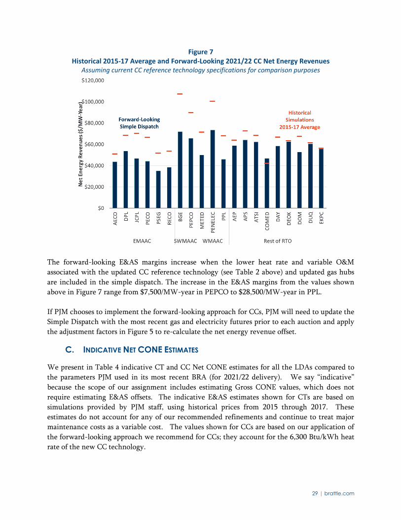
29 | brattle.com

Figure 7 Historical 2015-17 Average and Forward-Looking 2021/22 CC Net Energy Revenues

Assuming current CC reference technology specifications for comparison purposes

The forward-looking E&AS margins increase when the lower heat rate and variable O&M

associated with the updated CC reference technology (see Table 2 above) and updated gas hubs

are included in the simple dispatch. The increase in the E&AS margins from the values shown

above in Figure 7 range from $7,500/MW-year in PEPCO to $28,500/MW-year in PPL.

If PJM chooses to implement the forward-looking approach for CCs, PJM will need to update the

Simple Dispatch with the most recent gas and electricity futures prior to each auction and apply

the adjustment factors in Figure 5 to re-calculate the net energy revenue offset.

C. INDICATIVE NET CONE ESTIMATES

We present in Table 4 indicative CT and CC Net CONE estimates for all the LDAs compared to

the parameters PJM used in its most recent BRA (for 2021/22 delivery). We say “indicative”

because the scope of our assignment includes estimating Gross CONE values, which does not

require estimating E&AS offsets. The indicative E&AS estimates shown for CTs are based on

simulations provided by PJM staff, using historical prices from 2015 through 2017. These

estimates do not account for any of our recommended refinements and continue to treat major

maintenance costs as a variable cost. The values shown for CCs are based on our application of

the forward-looking approach we recommend for CCs; they account for the 6,300 Btu/kWh heat

rate of the new CC technology.

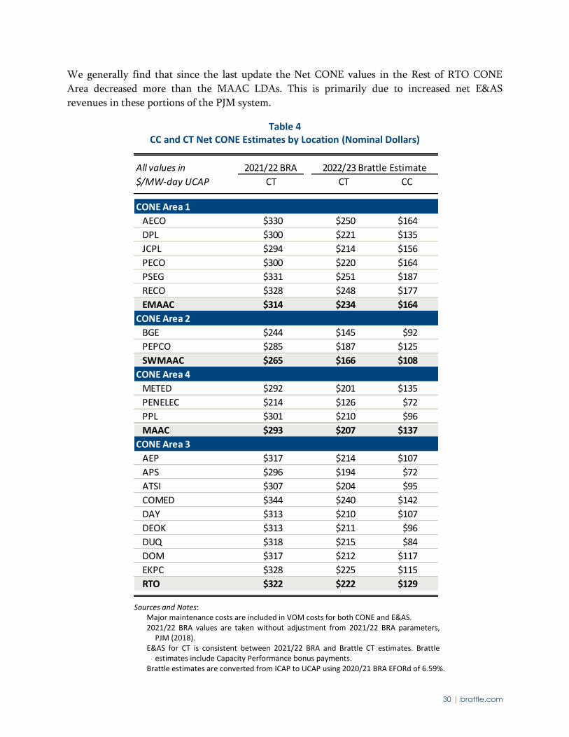
30 | brattle.com

We generally find that since the last update the Net CONE values in the Rest of RTO CONE

Area decreased more than the MAAC LDAs. This is primarily due to increased net E&AS

revenues in these portions of the PJM system.

Table 4 CC and CT Net CONE Estimates by Location (Nominal Dollars)

Sources and Notes:

Major maintenance costs are included in VOM costs for both CONE and E&AS. 2021/22 BRA values are taken without adjustment from 2021/22 BRA parameters,

PJM (2018). E&AS for CT is consistent between 2021/22 BRA and Brattle CT estimates. Brattle

estimates include Capacity Performance bonus payments. Brattle estimates are converted from ICAP to UCAP using 2020/21 BRA EFORd of 6.59%.

All values in 2021/22 BRA 2022/23 Brattle Estimate

$/MW-day UCAP CT CT CC

CONE Area 1

AECO $330 $250 $164

DPL $300 $221 $135

JCPL $294 $214 $156

PECO $300 $220 $164

PSEG $331 $251 $187

RECO $328 $248 $177

EMAAC $314 $234 $164

CONE Area 2

BGE $244 $145 $92

PEPCO $285 $187 $125

SWMAAC $265 $166 $108

CONE Area 4

METED $292 $201 $135

PENELEC $214 $126 $72

PPL $301 $210 $96

MAAC $293 $207 $137

CONE Area 3

AEP $317 $214 $107

APS $296 $194 $72

ATSI $307 $204 $95

COMED $344 $240 $142

DAY $313 $210 $107

DEOK $313 $211 $96

DUQ $318 $215 $84

DOM $317 $212 $117

EKPC $328 $225 $115

RTO $322 $222 $129

31 | brattle.com

D. CONSTRUCTION OF “RTO-WIDE” NET CONE FOR THE SYSTEM VRR CURVE

PJM’s current approach to estimating RTO Net CONE consists of two steps. First, PJM calculates

the RTO Gross CONE parameter by taking the simple average of Gross CONE values across the

four CONE areas. Second, PJM estimates net E&AS revenues by running its dispatch model for a

hypothetical unit purchasing gas at an appropriate pricing point and earning the average LMP

across the footprint. While PJM’s approach to calculating RTO Gross CONE is reasonable, we

recommend that PJM modify its calculation of RTO net E&AS revenues and estimate this

parameter as the median of net E&AS revenues across LDAs. Similarly, we recommend that PJM

estimate net E&AS revenues for each multi-zone LDA (e.g., MAAC, EMAAC) as the median of

net E&AS revenues across LDAs within the multi-zone LDA.

The major drawback of PJM’s current approach to estimating RTO E&AS margins is that it uses

gas and electricity prices that are not consistent with each other and thus might express false

price spreads. E&AS margins estimated using these prices are not earned by any actual resource

and might be higher or lower than a representative LDA. For all auctions since 2018/19, RTO

E&AS offsets have been 18-26% lower than the average E&AS margin across zones, and 7-20%

lower than the median E&AS margin. Under current market conditions, it therefore appears that

PJM’s current approach may underestimate E&AS margins. However, under other market

conditions, the approach could over-estimate E&AS margins, leading to under-procurement and

reliability challenges.

There are several advantages to using the median instead of the average LDA value to set the

RTO E&AS parameter. First, this approach should yield an approximately efficient result under

equilibrium conditions. Under equilibrium conditions, import-constrained LDAs will have

higher Net CONE than their parents, and will likely have lower E&AS margins. The median

E&AS margin will not be affected by a small number of LDAs with very low E&AS margins, and

will therefore contribute to providing the right incentive for investment in the unconstrained

portion of the system.

Second, the median should be relatively robust under conditions that deviate from equilibrium.

Under conditions where some LDAs have abnormally high E&AS values in the short-run, the

median value will not be affected. This will keep Net CONE high enough to support investment

in the rest of the footprint. The median approach also provides a measure of protection from

administrative error in estimating E&AS margins that may occur in some LDAs due to the small

sample of units to choose from or the difficulty of fully capturing locational varying costs and

energy prices. Using the median value prevents RTO Net CONE from being unduly influenced

by such errors and results in a more stable estimate over time.

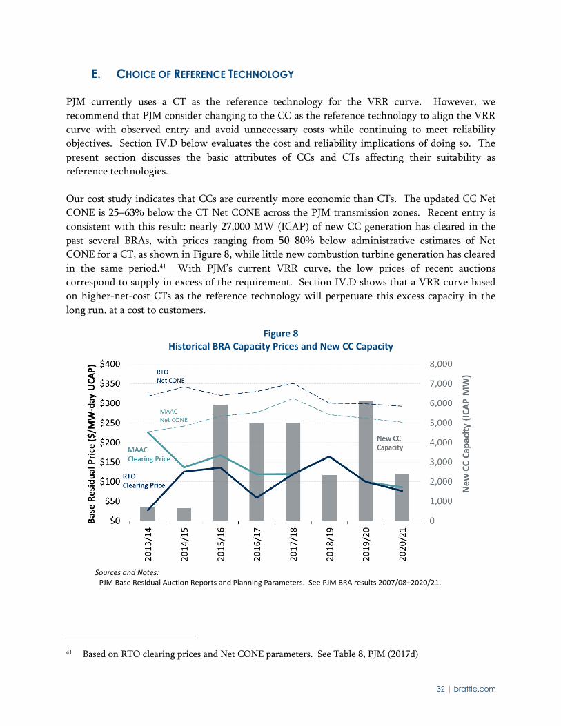
32 | brattle.com

E. CHOICE OF REFERENCE TECHNOLOGY

PJM currently uses a CT as the reference technology for the VRR curve. However, we

recommend that PJM consider changing to the CC as the reference technology to align the VRR

curve with observed entry and avoid unnecessary costs while continuing to meet reliability

objectives. Section IV.D below evaluates the cost and reliability implications of doing so. The

present section discusses the basic attributes of CCs and CTs affecting their suitability as

reference technologies.

Our cost study indicates that CCs are currently more economic than CTs. The updated CC Net

CONE is 25–63% below the CT Net CONE across the PJM transmission zones. Recent entry is

consistent with this result: nearly 27,000 MW (ICAP) of new CC generation has cleared in the

past several BRAs, with prices ranging from 50–80% below administrative estimates of Net

CONE for a CT, as shown in Figure 8, while little new combustion turbine generation has cleared

in the same period.41 With PJM’s current VRR curve, the low prices of recent auctions

correspond to supply in excess of the requirement. Section IV.D shows that a VRR curve based

on higher-net-cost CTs as the reference technology will perpetuate this excess capacity in the

long run, at a cost to customers.

Figure 8 Historical BRA Capacity Prices and New CC Capacity

Sources and Notes:

PJM Base Residual Auction Reports and Planning Parameters. See PJM BRA results 2007/08–2020/21.

41 Based on RTO clearing prices and Net CONE parameters. See Table 8, PJM (2017d)

33 | brattle.com

Another consideration is the ability to estimate Net CONE accurately. The conventional wisdom

has always been that CCs are subject to more estimation error in E&AS offsets, since their E&AS

offsets are larger. We disagree. The benchmark for “accuracy” should be the value that investors

anticipate in the market. That benchmark is not directly observable, but there is more market

data available to anticipate E&AS offsets for CCs than CTs. As we showed above, CCs’ net E&AS

revenues can be accurately approximated based on 5x16 operation, and futures prices for 5x16

on-peak blocks are observable in the market. No such benchmark is available for CTs, so we rely

on historical estimates that may not be representative of the future delivery year due to historical

anomalies and evolving market conditions. Finally, CTs face less transparent gas procurement

costs since they are committed and dispatched day-of, as discussed in Section II.B above.

A separate issue from forecast error is volatility. In theory, CC E&AS offsets and Net CONE

values vary more than they do for CTs as market conditions fluctuate. This could potentially

increase capacity price volatility and adversely affect capacity resources, such as demand

response, that do not earn meaningful net energy revenues. However, forward-looking E&AS

offsets for CCs avoid the volatility seen in historically-based E&AS offsets for CTs when

anomalies such as the Polar Vortex occur. Such anomalies are presumed to be implicitly

included in futures prices with appropriate weightings on their future probability, as determined

by the market. Indeed, the use of forward-looking E&AS offsets for CCs could reduce volatility

relative to historical offsets used for CTs.

We and other analysts have long cautioned against repeatedly switching to the current lowest

cost reference technology in a market where Net CONE for each resource type may fluctuate

from year to year around its long-run equilibrium value. This practice would suppress long-run

average administrative Net CONE below long-run average actual Net CONE, resulting in VRR

curve prices too low to sustain investment consistent with target reserve margins. We believe,

however, that the cost advantage of CCs reflects fundamental long-term cost drivers, rather than

a temporary deviation from equilibrium. CCs have been the dominant technology for many

years. While this was also the case during the previous VRR curve review in 2014, an additional

four BRAs with even greater CC entry and limited CT entry has further emphasized the shift in

the market. Going forward, their substantial heat rate advantage relative to CTs should

overcome their slightly higher Gross CONE on a per-kW basis. The convergence of the Gross

CONE between the two resource types since the 2014 review means that CCs are likely to

remain more cost effective under wide ranging market conditions. It is conceivable that CTs

could become economic in a high-renewable future where their flexibility is more highly valued

and the energy value of CCs is lower.42 However, it is unlikely that CTs will become strictly

42 In our 2014 Review, we stated that any technology that is economically viable in the long run could

be selected for determining Net CONE. We continue to believe this. However, given the tremendous

net cost advantage of CCs and recent new entry evidence in the market, it is not clear that CTs will

remain part of the supply mix in equilibrium.

34 | brattle.com

more economic over several auctions and that PJM (or intervenors) will then be tempted to

switch back the reference technology.

We understand that ISO-NE recently switched its reference technology from a CC to a CT after

they estimated that CT Net CONE was 20% below CC Net CONE in New England, its auction

cleared a frame-type CT, and they passed market reforms that favor fast-start and flexible

resources. The FERC accepted ISO-NE’s request on the basis that Net CONE for the lowest cost

commercially available resource is high enough to incentivize new entry, but not so high that

customers incur unnecessary costs. In contrast to ISO-NE’s findings in New England, our CONE

study suggests that CCs are less expensive than CTs in PJM, and CCs are the strongly dominant

technology of actual entrants. Our recommendation that PJM adopt a CC as the reference

technology aims to achieve the same outcomes that the FERC approved for New England:

attracting new entry without driving up customer costs unnecessarily.43

43 ISO New England, Inc., (2017). “RE: ISO New England Inc.; Filing of CONE and ORTP Updates,”

January 13, 2017. Docket No. ER17-795-000.

35 | brattle.com

III. Probabilistic Simulation Approach

The position, slope, and shape of PJM’s VRR curve have consequences for realized reliability

levels and price volatility in the capacity market. The parameters of the VRR curve determine

the expected distribution of price and quantity outcomes, but these effects are not observable in

historical market outcomes with only a few years of historical experience. We therefore use a

Monte Carlo model to simulate distributions of price, quantity, and reliability outcomes that

might be realized over many years under PJM’s current VRR curve or alternative curves. We

describe here the primary components of this model, including our characterization of supply,

demand, transmission, reliability, and locational auction clearing. We describe how we enhance

our approach to account for the substantial impact of Capacity Performance on the shape of the

RPM supply curve and how it affects our modeling.

A. MODEL STRUCTURE

To evaluate the performance of the VRR curve and alternative curves in long-run equilibrium,

we conduct a Monte Carlo simulation of capacity market outcomes. This analysis allows us to

estimate distributions of price, quantity, and reliability outcomes under a particular VRR curve,

and review these outcomes in light of the performance objectives of the VRR curve and RPM.

The Monte Carlo simulation model we employ in this analysis is an enhanced version of the

model used in our 2014 VRR curve report.44 We originally developed the model to represent the

characteristics of PJM’s RPM. We calibrate the size and standard deviations of fluctuations in

supply and demand, at the RTO level and within each LDA, to levels observed historically in

PJM. The model uses a realistic sloped supply curve that is calibrated based on RPM offers and

reflects the wide range of capacity resources bidding into the market. The model realistically

accounts for the impact of Capacity Performance on the supply curve. It captures the range of

expectations of performance risk across market participants and the resulting increase in supply

curve prices at the low end of the price range.

We use the planning parameters for delivery year 2020/21 as the basis for our modeling

assumptions, combined with historically-grounded locational supply curves, to determine

locational clearing prices and quantities. We also evaluate performance of PJM’s VRR using

updated Gross and Net CONE values from our concurrently released CONE study. We then use

historical market data to develop realistic fluctuations to supply, demand, and transmission in

each draw. A stylized depiction of the price and quantity distributions driven by supply and

44 A similar model was originally developed by Professor Benjamin Hobbs to evaluate VRR curve

performance and we have used variants of this model to help develop and evaluate capacity market

demand curves for ISO-New England (ISO-NE), the Alberta Electricity System Operator (AESO), and

the Midcontinent ISO (MISO). See discussion of the Hobbs simulation model in our 2008, 2011, and

2014 RPM Reports, Pfeifenberger et al. (2008, 2011, and 2014).

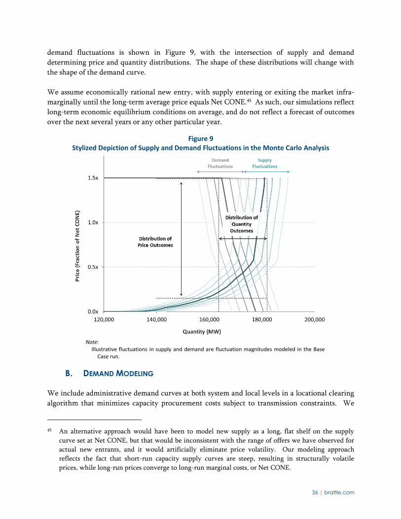
36 | brattle.com

demand fluctuations is shown in Figure 9, with the intersection of supply and demand

determining price and quantity distributions. The shape of these distributions will change with

the shape of the demand curve.

We assume economically rational new entry, with supply entering or exiting the market infra-

marginally until the long-term average price equals Net CONE.45 As such, our simulations reflect

long-term economic equilibrium conditions on average, and do not reflect a forecast of outcomes

over the next several years or any other particular year.

Figure 9 Stylized Depiction of Supply and Demand Fluctuations in the Monte Carlo Analysis

Note:

Illustrative fluctuations in supply and demand are fluctuation magnitudes modeled in the Base Case run.

B. DEMAND MODELING

We include administrative demand curves at both system and local levels in a locational clearing

algorithm that minimizes capacity procurement costs subject to transmission constraints. We

45 An alternative approach would have been to model new supply as a long, flat shelf on the supply

curve set at Net CONE, but that would be inconsistent with the range of offers we have observed for

actual new entrants, and it would artificially eliminate price volatility. Our modeling approach

reflects the fact that short-run capacity supply curves are steep, resulting in structurally volatile

prices, while long-run prices converge to long-run marginal costs, or Net CONE.

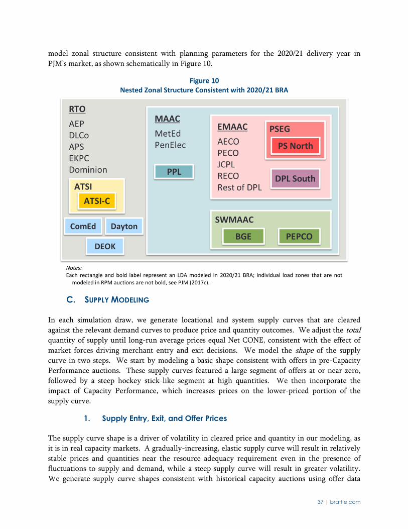
37 | brattle.com

model zonal structure consistent with planning parameters for the 2020/21 delivery year in

PJM’s market, as shown schematically in Figure 10.

Figure 10 Nested Zonal Structure Consistent with 2020/21 BRA

Notes: Each rectangle and bold label represent an LDA modeled in 2020/21 BRA; individual load zones that are not

modeled in RPM auctions are not bold, see PJM (2017c).

C. SUPPLY MODELING

In each simulation draw, we generate locational and system supply curves that are cleared

against the relevant demand curves to produce price and quantity outcomes. We adjust the total quantity of supply until long-run average prices equal Net CONE, consistent with the effect of

market forces driving merchant entry and exit decisions. We model the shape of the supply

curve in two steps. We start by modeling a basic shape consistent with offers in pre-Capacity

Performance auctions. These supply curves featured a large segment of offers at or near zero,

followed by a steep hockey stick-like segment at high quantities. We then incorporate the

impact of Capacity Performance, which increases prices on the lower-priced portion of the

supply curve.

1. Supply Entry, Exit, and Offer Prices

The supply curve shape is a driver of volatility in cleared price and quantity in our modeling, as

it is in real capacity markets. A gradually-increasing, elastic supply curve will result in relatively

stable prices and quantities near the resource adequacy requirement even in the presence of

fluctuations to supply and demand, while a steep supply curve will result in greater volatility.

We generate supply curve shapes consistent with historical capacity auctions using offer data

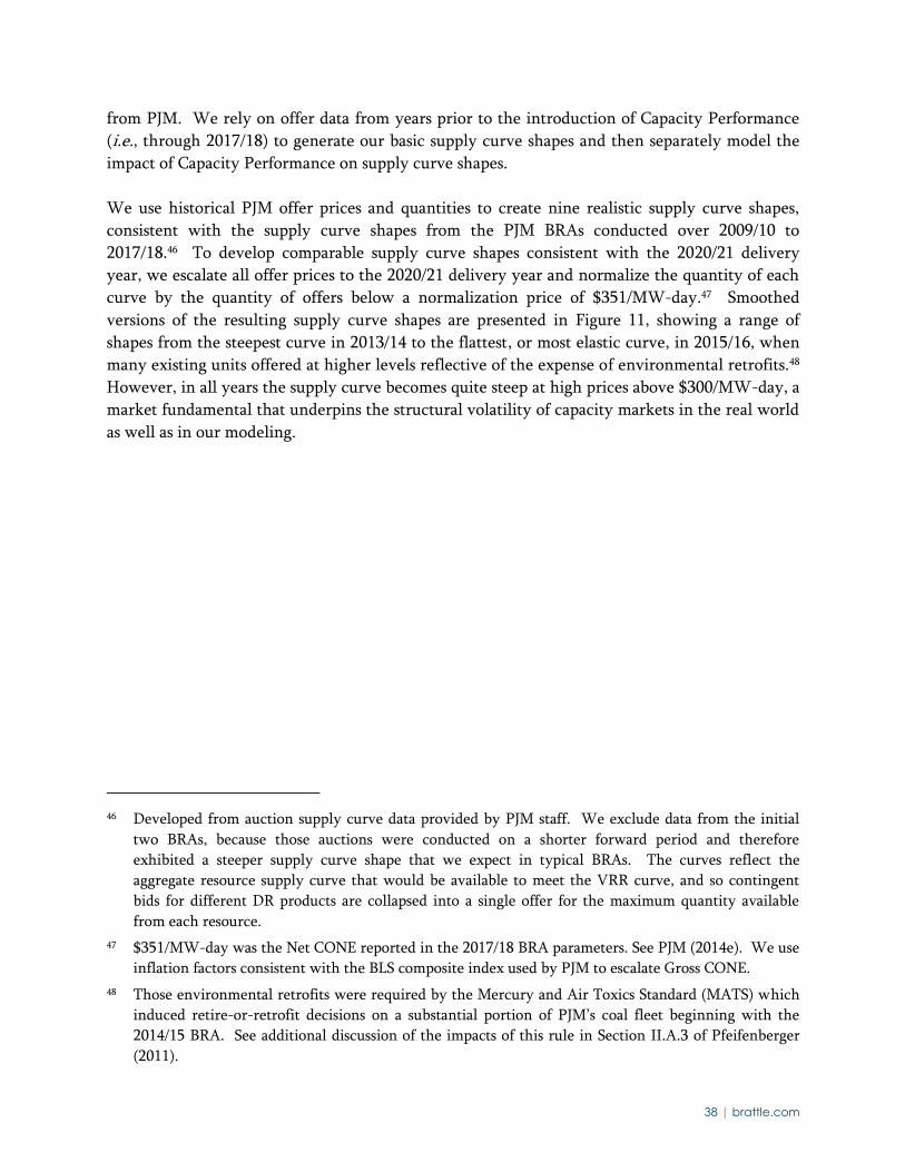
38 | brattle.com

from PJM. We rely on offer data from years prior to the introduction of Capacity Performance

(i.e., through 2017/18) to generate our basic supply curve shapes and then separately model the

impact of Capacity Performance on supply curve shapes.

We use historical PJM offer prices and quantities to create nine realistic supply curve shapes,

consistent with the supply curve shapes from the PJM BRAs conducted over 2009/10 to

2017/18.46 To develop comparable supply curve shapes consistent with the 2020/21 delivery

year, we escalate all offer prices to the 2020/21 delivery year and normalize the quantity of each

curve by the quantity of offers below a normalization price of $351/MW-day.47 Smoothed

versions of the resulting supply curve shapes are presented in Figure 11, showing a range of

shapes from the steepest curve in 2013/14 to the flattest, or most elastic curve, in 2015/16, when

many existing units offered at higher levels reflective of the expense of environmental retrofits.48

However, in all years the supply curve becomes quite steep at high prices above $300/MW-day, a

market fundamental that underpins the structural volatility of capacity markets in the real world

as well as in our modeling.

46 Developed from auction supply curve data provided by PJM staff. We exclude data from the initial

two BRAs, because those auctions were conducted on a shorter forward period and therefore

exhibited a steeper supply curve shape that we expect in typical BRAs. The curves reflect the

aggregate resource supply curve that would be available to meet the VRR curve, and so contingent

bids for different DR products are collapsed into a single offer for the maximum quantity available

from each resource.

47 $351/MW-day was the Net CONE reported in the 2017/18 BRA parameters. See PJM (2014e). We use

inflation factors consistent with the BLS composite index used by PJM to escalate Gross CONE.

48 Those environmental retrofits were required by the Mercury and Air Toxics Standard (MATS) which

induced retire-or-retrofit decisions on a substantial portion of PJM’s coal fleet beginning with the

2014/15 BRA. See additional discussion of the impacts of this rule in Section II.A.3 of Pfeifenberger

(2011).

39 | brattle.com

Figure 11 Individual Basic Supply Curve Shapes used in Monte Carlo Analysis

Sources and Notes: Smoothed supply offer curves developed from raw data provided by PJM staff.

Offer curves normalized by quantities offered below $351/MW-day and inflated to 2020/21 dollars.

We reflect the lumpy nature of investments by simulating each supply curve as a collection of

discrete offer blocks. Simply modeling a smooth offer curve, like one of the individual smoothed

curves shown in Figure 11, would somewhat understate realized volatility in price and quantity

outcomes, especially in small LDAs that are more greatly affected by lumpy investments. To

derive realistically-sized offer blocks in each location, we randomly select from actual offers in

that location from the 2017/18 BRA but re-price those offers consistent with the selected smooth

supply curve shape.

To simulate rational economic entry, we increase or decrease the quantity of zero-priced supply

so that the average clearing price over all draws is equal to Net CONE.49 The result is that

average-clearing prices will always converge to Net CONE under all possible demand curves,

although differently-shaped demand curves will result in different average-cleared quantities.

This approach allows us to examine the performance of the VRR curve in a long-term

49 In the second step of our supply curve modeling, many of the zero-priced offers rise above zero,

consistent with Capacity Performance offers in the 2018/19 through 2020/21 BRAs.

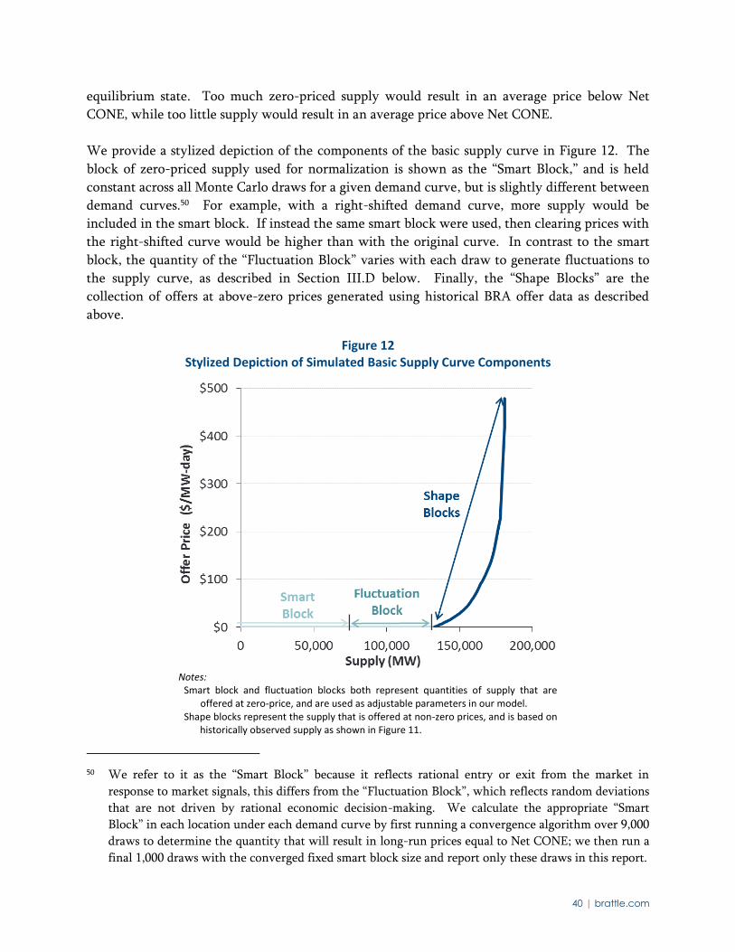
40 | brattle.com

equilibrium state. Too much zero-priced supply would result in an average price below Net

CONE, while too little supply would result in an average price above Net CONE.

We provide a stylized depiction of the components of the basic supply curve in Figure 12. The

block of zero-priced supply used for normalization is shown as the “Smart Block,” and is held

constant across all Monte Carlo draws for a given demand curve, but is slightly different between

demand curves.50 For example, with a right-shifted demand curve, more supply would be

included in the smart block. If instead the same smart block were used, then clearing prices with

the right-shifted curve would be higher than with the original curve. In contrast to the smart

block, the quantity of the “Fluctuation Block” varies with each draw to generate fluctuations to

the supply curve, as described in Section III.D below. Finally, the “Shape Blocks” are the

collection of offers at above-zero prices generated using historical BRA offer data as described

above.

Figure 12 Stylized Depiction of Simulated Basic Supply Curve Components

Notes: Smart block and fluctuation blocks both represent quantities of supply that are

offered at zero-price, and are used as adjustable parameters in our model. Shape blocks represent the supply that is offered at non-zero prices, and is based on

historically observed supply as shown in Figure 11.

50 We refer to it as the “Smart Block” because it reflects rational entry or exit from the market in

response to market signals, this differs from the “Fluctuation Block”, which reflects random deviations

that are not driven by rational economic decision-making. We calculate the appropriate “Smart

Block” in each location under each demand curve by first running a convergence algorithm over 9,000

draws to determine the quantity that will result in long-run prices equal to Net CONE; we then run a

final 1,000 draws with the converged fixed smart block size and report only these draws in this report.

41 | brattle.com

2. Supply Curve Adjustments for Capacity Performance

Following capacity shortfalls during the 2014 Polar Vortex, PJM developed the Capacity

Performance construct to ensure that the RPM delivered the expected level of reliability.

Capacity Performance created significantly stronger incentives for resources committed in the

capacity auction to meet their obligations. It also compensated resources choosing to forego

capacity obligations by providing bonus payments on their full output during performance

events. Capacity Performance has significant implications for how the RPM will function going

forward because of how it affects offer price incentives and reliability outcomes under a given

demand curve. To enhance our modeling approach, we use a combination of economic theory

and analysis of auction data to gain a detailed understanding of how offer behavior is changing

with Capacity Performance.

To understand the impact of Capacity Performance on supply curves, we analyzed BRA offer

data before and after Capacity Performance was implemented. The available data included offers

from the non-Capacity Performance auctions (2007/08–2017/18 BRAs) and the Capacity

Performance auctions (2018/19–2020/21 BRAs).51 Figure 13 compares supply curves from the

recent Capacity Performance auctions (indicated by the colored lines) to pre-Capacity

Performance supply curves (grey lines) and shows how offers have changed. The Capacity

Performance supply curves have fewer zero-priced offers and more offers with gradually

increasing prices compared to earlier curves. Offers in the low-priced portion of the curve have

increased on average, reflecting the opportunity cost of foregone bonus payments that will be

discussed below.

51 The first Capacity Performance auctions were conducted in 2015, when PJM held the 2018/19 BRA

and two special transitional auctions to procure Capacity Performance resources for the 2016/17 and

2017/18 delivery years. In the 2018/19 and the 2019/20 BRAs, PJM procured both Capacity

Performance resources (subject to a minimum quantity constraint) and “Base” resources, which were

not subject to performance penalties. Resources could choose to offer as either type, with Capacity

Performance resources receiving a premium above the Base price. PJM set targets of procuring

Capacity Performance resources up to 60% and 70% of the reliability requirement for the 2016/17 and

2017/18 Transition Auctions, respectively. Starting with the 2020/21 BRA, PJM procured only the

Capacity Performance product. See PJM (2015c).

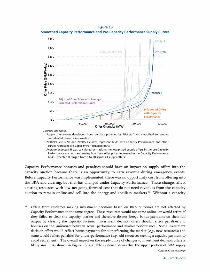
42 | brattle.com

Figure 13 Smoothed Capacity Performance and Pre-Capacity Performance Supply Curves

Sources and Notes:

Supply offer curves developed from raw data provided by PJM staff and smoothed to remove confidential resource information.

2018/19, 2019/20, and 2020/21 curves represent BRAs with Capacity Performance and other curves represent pre-Capacity Performance BRAs.

Average expected H was calculated by tracking the low-priced supply offers in the pre-Capacity Performance auctions and seeing how their offer prices increased in the Capacity Performance BRAs. Expected H ranged from 0 to 30 across all supply offers.

Capacity Performance bonuses and penalties should have an impact on supply offers into the

capacity auction because there is an opportunity to earn revenue during emergency events.

Before Capacity Performance was implemented, there was no opportunity cost from offering into

the BRA and clearing, but that has changed under Capacity Performance. These changes affect

existing resources with low net going-forward cost that do not need revenues from the capacity

auction to remain online and sell into the energy and ancillary markets.52 Without a capacity

52 Offers from resources making investment decisions based on BRA outcomes are not affected by

Capacity Performance to the same degree. These resources would not come online, or would retire, if

they failed to clear the capacity market and therefore do not forego bonus payments on their full

output by clearing the capacity auction. Investment decision offers should reflect penalties and

bonuses on the difference between actual performance and market performance. Some investment

decision offers would reflect bonus payments for outperforming the market (e.g., new resources) and

some would reflect penalties for under-performance (e.g., old resources seeking a capacity payment to

avoid retirement). The overall impact on the supply curve of changes to investment decision offers is

likely small. As shown in Figure 13, available evidence shows that the upper portion of BRA supply

Continued on next page

43 | brattle.com

obligation, these resources would earn bonus payments on their full output during performance

hours. With a capacity obligation, they forego bonus payments on the balancing ratio (since

they receive payments based on the difference between their performance and the balancing

ratio). In order to ensure they break even by taking on a capacity obligation, these resources will

offer their foregone bonus payments into the auction, as shown in Figure 14.

Figure 14 shows expected supply offers for different types of resources after accounting for

Capacity Performance incentives. Resources with zero or low net going-forward cost are

expected to submit a “Bonus Opportunity Cost Offer”. As explained above, these resources will

include the opportunity cost of foregoing bonus payments on their full output in their offer

price. We directly model the impact of these offers on the lower part of the supply curve. New

resources (or resources considering mothballing or retiring) will submit an “Investment Decision

Offer.” Since their participation in the market is contingent on clearing the capacity auction,

supply offers from these resources will only be adjusted by the amount of penalty or bonus

payments they expect to receive on the difference between their output and the market average.

Because the adjustments will be small and offsetting between different resources, we do not

directly model the impact of these offers on the upper portion of the supply curve.53

Continued from previous page

curves (above around $200/MW-day) do not appear to have changed with the introduction of

Capacity Performance.

53 Investment Decision Offers will be greater than Net Going Forward costs for resources expecting to

under-perform the market and less than Net Going Forward Cost for resources expecting to over-

perform the market.

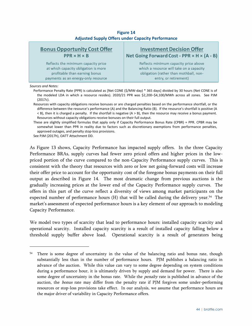
44 | brattle.com

Figure 14 Adjusted Supply Offers under Capacity Performance

Sources and Notes:

Performance Penalty Rate (PPR) is calculated as [Net CONE ($/MW-day) * 365 days] divided by 30 hours (Net CONE is of the modeled LDA in which a resource resides). 2020/21 PPR was $2,200–$4,100/MWh across all zones. See PJM (2017c).

Resources with capacity obligations receive bonuses or are charged penalties based on the performance shortfall, or the difference between the resource’s performance (A) and the Balancing Ratio (B). If the resource’s shortfall is positive (A < B), then it is charged a penalty. If the shortfall is negative (A > B), then the resource may receive a bonus payment. Resources without capacity obligations receive bonuses on their full output.

These are slightly simplified formulas that apply only if Capacity Performance Bonus Rate (CPBR) = PPR. CPBR may be somewhat lower than PPR in reality due to factors such as discretionary exemptions from performance penalties, approved outages, and penalty stop-loss provisions.

See PJM (2017h), OATT Attachment DD.

As Figure 13 shows, Capacity Performance has impacted supply offers. In the three Capacity

Performance BRAs, supply curves had fewer zero priced offers and higher prices in the low-

priced portion of the curve compared to the non-Capacity Performance supply curves. This is

consistent with the theory that resources with zero or low net going-forward costs will increase

their offer price to account for the opportunity cost of the foregone bonus payments on their full

output as described in Figure 14. The most dramatic change from previous auctions is the

gradually increasing prices at the lower end of the Capacity Performance supply curves. The

offers in this part of the curve reflect a diversity of views among market participants on the

expected number of performance hours (H) that will be called during the delivery year.54 The

market’s assessment of expected performance hours is a key element of our approach to modeling

Capacity Performance.

We model two types of scarcity that lead to performance hours: installed capacity scarcity and

operational scarcity. Installed capacity scarcity is a result of installed capacity falling below a

threshold supply buffer above load. Operational scarcity is a result of generators being

54 There is some degree of uncertainty in the value of the balancing ratio and bonus rate, though

substantially less than in the number of performance hours. PJM publishes a balancing ratio in

advance of the auction. While this value can vary to some degree depending on system conditions

during a performance hour, it is ultimately driven by supply and demand for power. There is also

some degree of uncertainty in the bonus rate. While the penalty rate is published in advance of the

auction, the bonus rate may differ from the penalty rate if PJM forgives some under-performing

resources or stop-loss provisions take effect. In our analysis, we assume that performance hours are

the major driver of variability in Capacity Performance offers.

45 | brattle.com

unavailable to operate to meet their obligations. For example, during the 2014 Polar Vortex, PJM

had sufficient installed capacity to meet load but many plants were not available due to fuel

supply or other operability constraints.

To assess installed capacity scarcity, we relied on reliability modeling data from PJM. We found

that at equilibrium reserve margins, two to three performance hours are expected during an

average year due to installed capacity scarcity. Due to the high reserve margins in PJM over the

last few years, installed capacity scarcity performance hours were very unlikely. Most past

performance events were due to operational scarcity. Using historical performance events data

posted by PJM, we estimated that about seven performance hours are expected annually due to

operational scarcity. Based on offer data provided by PJM, market participants expect ten

performance hours on average, ranging from 0 to 30 across all participants.

We model the range of market participant expectations of H based on offers in the 2018/19

through 2020/21 Capacity Performance auctions. As we describe in more detail in Appendix B,

we estimate implied performance hours in each Capacity Performance offer across these three

auctions. We then fit a mixture distribution consisting of offers with zero performance hours

and beta-distributed offers with performance hours between zero and 30.

Figure 15 shows a stylized depiction of our approach to generating Capacity Performance supply

curves in our Monte Carlo modeling. The horizontal dashed lines of the figure show the average

impact of installed capacity and operational scarcity on offers. The sloped lines of the figure

shows the range of market participant expectations of H based on our statistical model. For each

draw, we determine installed capacity scarcity performance hours based on the supply cushion in

that draw, generate random operating scarcity performance hours, and then apply our statistical

model to determine the dispersion of performance hours across offers. We then convert the

performance hours into offers by multiplying by the penalty rate and the balancing ratio. For

more detail on our Capacity Performance modeling, see Appendix B.

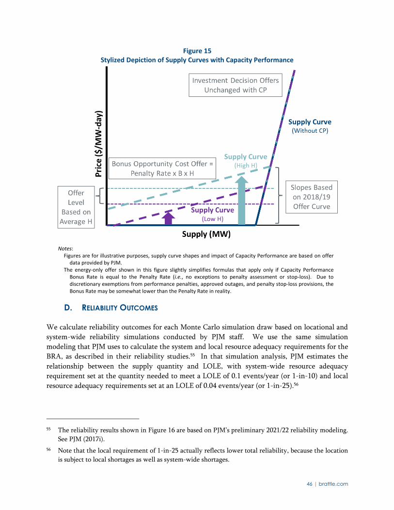
46 | brattle.com

Figure 15 Stylized Depiction of Supply Curves with Capacity Performance

Notes:

Figures are for illustrative purposes, supply curve shapes and impact of Capacity Performance are based on offer data provided by PJM.

The energy-only offer shown in this figure slightly simplifies formulas that apply only if Capacity Performance Bonus Rate is equal to the Penalty Rate (i.e., no exceptions to penalty assessment or stop-loss). Due to discretionary exemptions from performance penalties, approved outages, and penalty stop-loss provisions, the Bonus Rate may be somewhat lower than the Penalty Rate in reality.

D. RELIABILITY OUTCOMES

We calculate reliability outcomes for each Monte Carlo simulation draw based on locational and

system-wide reliability simulations conducted by PJM staff. We use the same simulation

modeling that PJM uses to calculate the system and local resource adequacy requirements for the

BRA, as described in their reliability studies.55 In that simulation analysis, PJM estimates the

relationship between the supply quantity and LOLE, with system-wide resource adequacy

requirement set at the quantity needed to meet a LOLE of 0.1 events/year (or 1-in-10) and local

resource adequacy requirements set at an LOLE of 0.04 events/year (or 1-in-25).56

55 The reliability results shown in Figure 16 are based on PJM’s preliminary 2021/22 reliability modeling.

See PJM (2017i).

56 Note that the local requirement of 1-in-25 actually reflects lower total reliability, because the location

is subject to local shortages as well as system-wide shortages.

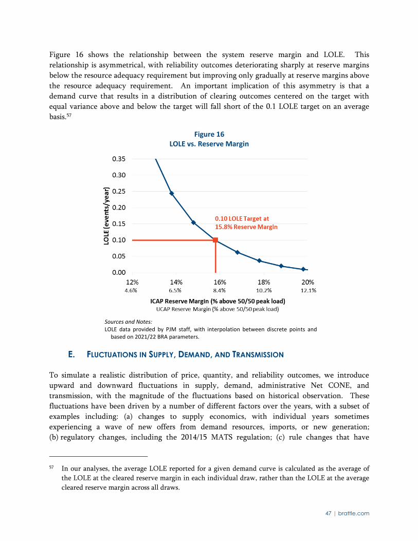
47 | brattle.com

Figure 16 shows the relationship between the system reserve margin and LOLE. This

relationship is asymmetrical, with reliability outcomes deteriorating sharply at reserve margins

below the resource adequacy requirement but improving only gradually at reserve margins above

the resource adequacy requirement. An important implication of this asymmetry is that a

demand curve that results in a distribution of clearing outcomes centered on the target with

equal variance above and below the target will fall short of the 0.1 LOLE target on an average

basis.57

Figure 16 LOLE vs. Reserve Margin

Sources and Notes: LOLE data provided by PJM staff, with interpolation between discrete points and

based on 2021/22 BRA parameters.

E. FLUCTUATIONS IN SUPPLY, DEMAND, AND TRANSMISSION

To simulate a realistic distribution of price, quantity, and reliability outcomes, we introduce

upward and downward fluctuations in supply, demand, administrative Net CONE, and

transmission, with the magnitude of the fluctuations based on historical observation. These

fluctuations have been driven by a number of different factors over the years, with a subset of

examples including: (a) changes to supply economics, with individual years sometimes

experiencing a wave of new offers from demand resources, imports, or new generation;

(b) regulatory changes, including the 2014/15 MATS regulation; (c) rule changes that have

57 In our analyses, the average LOLE reported for a given demand curve is calculated as the average of

the LOLE at the cleared reserve margin in each individual draw, rather than the LOLE at the average

cleared reserve margin across all draws.

48 | brattle.com

resulted in increased or decreased offer quantities from categories of resources such as demand

response and imports; (d) the economic recession that began in 2007, resulting in a substantial

reduction in demand forecasts over the subsequent years; and (e) incorporation of supply and

demand from FRR entities and territory expansions, which have tended to increase both supply

and demand by similar but not exactly offsetting magnitudes, thereby introducing a net supply

fluctuation into the market.

Because the magnitude of these fluctuations is an important driver of the performance of the

VRR curve, we report the sensitivity of the VRR curve’s performance to each type of fluctuation

and conduct a sensitivity analysis regarding overall fluctuations sizes in Section IV below. We

briefly describe here our approach to estimating fluctuations reflective of historical market data,

and provide additional detail supporting these estimates in Appendix A.

Supply: We estimate fluctuations in supply using the total quantity of supply

offered in each location during each historical BRA. We de-trend the historical

supply offer data and calculate deviations from the trend for each LDA. We use

these deviations to determine a relationship between LDA size and deviation size

and use this relationship to determine supply deviation sizes in each LDA.

Reliability Requirement: We estimate fluctuations in reliability requirement in

LDAs using a two-component model consisting of: (1) an RTO-correlated

fluctuation that is entirely driven by the variation in historical RTO reliability

requirements; and (2) an incremental fluctuation driven by variability in

historical reliability requirements above the RTO value for each LDA.

Administrative Net CONE: We assume that administrative Net CONE is subject

to random error around its expected value. We estimate the fluctuations in

administrative Net CONE in each simulation considering fluctuations in Gross

CONE, based on historical variation in PJM’s BLS Composite Index, minus

fluctuations in historical E&AS estimates.58

Capacity Emergency Transfer Limit: We simulate fluctuations in CETL as

normally distributed with a standard deviation of 15% of the expected CETL value

based on the 2020/21 parameters, with the standard deviation estimated based on

historical auction data across all locations and years.

The aggregate impact of these individual fluctuations is illustrated in Table 5, where we compare

historical fluctuations in net supply, both in terms of absolute value as well as de-trended values,

to the simulated fluctuations. This net supply comparison, calculated as supply plus CETL minus

reliability requirement, is the most important driver of price and quantity results in our

58 PJM’s Bureau of Labor Statistics composite index is comprised of the BLS Quarterly Census of

Employment and Wages for Utility System Construction (weighted 20%), the BLS Producer Index for

Construction Materials and Components (weighted 50%), and the BLS Producer Price Index for

Turbines and Turbine Generator Sets (weighted 30%). See PJM (2017f).

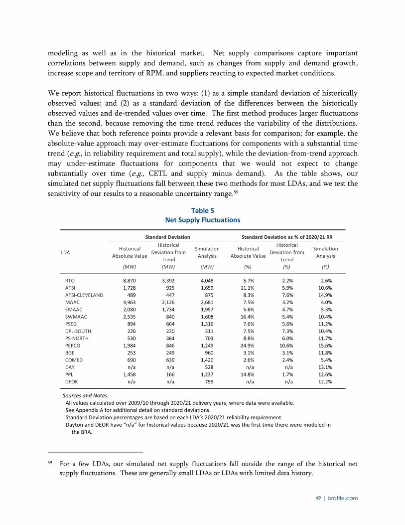
49 | brattle.com

modeling as well as in the historical market. Net supply comparisons capture important

correlations between supply and demand, such as changes from supply and demand growth,

increase scope and territory of RPM, and suppliers reacting to expected market conditions.

We report historical fluctuations in two ways: (1) as a simple standard deviation of historically

observed values; and (2) as a standard deviation of the differences between the historically

observed values and de-trended values over time. The first method produces larger fluctuations

than the second, because removing the time trend reduces the variability of the distributions.

We believe that both reference points provide a relevant basis for comparison; for example, the

absolute-value approach may over-estimate fluctuations for components with a substantial time

trend (e.g., in reliability requirement and total supply), while the deviation-from-trend approach

may under-estimate fluctuations for components that we would not expect to change

substantially over time (e.g., CETL and supply minus demand). As the table shows, our

simulated net supply fluctuations fall between these two methods for most LDAs, and we test the

sensitivity of our results to a reasonable uncertainty range.59

Table 5 Net Supply Fluctuations

Sources and Notes: All values calculated over 2009/10 through 2020/21 delivery years, where data were available. See Appendix A for additional detail on standard deviations. Standard Deviation percentages are based on each LDA’s 2020/21 reliability requirement.

Dayton and DEOK have “n/a” for historical values because 2020/21 was the first time there were modeled in the BRA.

59 For a few LDAs, our simulated net supply fluctuations fall outside the range of the historical net

supply fluctuations. These are generally small LDAs or LDAs with limited data history.

Standard Deviation Standard Deviation as % of 2020/21 RR

LDAHistorical

Absolute Value

Historical

Deviation from

Trend

Simulation

Analysis

Historical

Absolute Value

Historical

Deviation from

Trend

Simulation

Analysis

(MW) (MW) (MW) (%) (%) (%)

RTO 8,870 3,392 4,048 5.7% 2.2% 2.6%

ATSI 1,728 925 1,659 11.1% 5.9% 10.6%

ATSI-CLEVELAND 489 447 875 8.3% 7.6% 14.9%

MAAC 4,963 2,126 2,681 7.5% 3.2% 4.0%

EMAAC 2,080 1,734 1,957 5.6% 4.7% 5.3%

SWMAAC 2,535 840 1,608 16.4% 5.4% 10.4%

PSEG 894 664 1,316 7.6% 5.6% 11.2%

DPL-SOUTH 226 220 311 7.5% 7.3% 10.4%

PS-NORTH 530 364 703 8.8% 6.0% 11.7%

PEPCO 1,984 846 1,249 24.9% 10.6% 15.6%

BGE 253 249 960 3.1% 3.1% 11.8%

COMED 690 639 1,420 2.6% 2.4% 5.4%

DAY n/a n/a 528 n/a n/a 13.1%

PPL 1,458 166 1,237 14.8% 1.7% 12.6%

DEOK n/a n/a 799 n/a n/a 12.2%

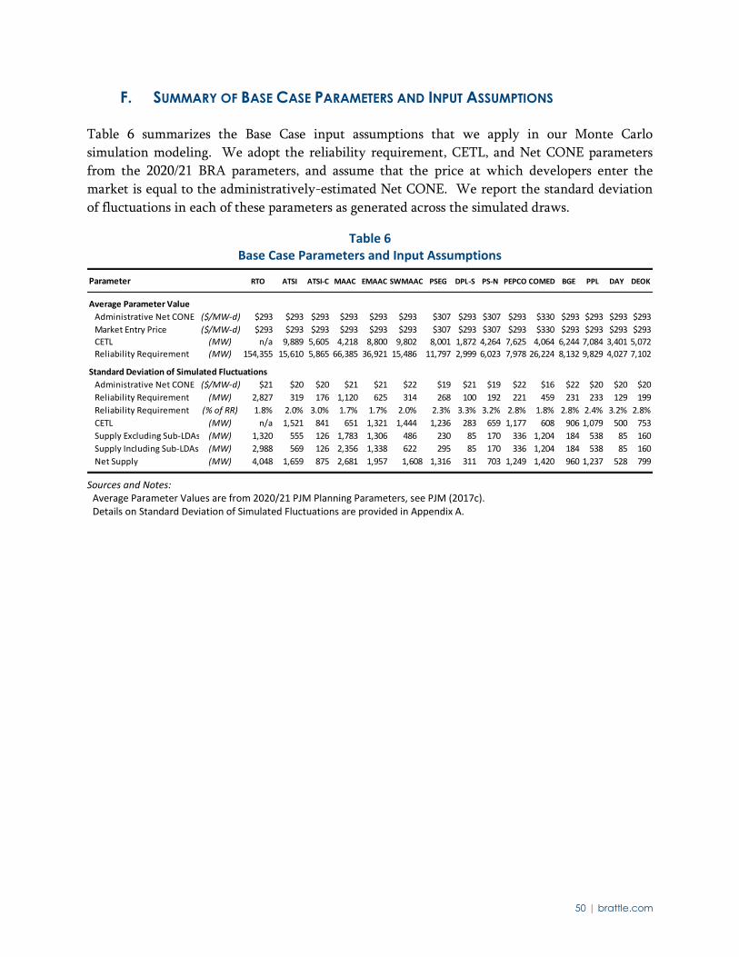
50 | brattle.com

F. SUMMARY OF BASE CASE PARAMETERS AND INPUT ASSUMPTIONS

Table 6 summarizes the Base Case input assumptions that we apply in our Monte Carlo

simulation modeling. We adopt the reliability requirement, CETL, and Net CONE parameters

from the 2020/21 BRA parameters, and assume that the price at which developers enter the

market is equal to the administratively-estimated Net CONE. We report the standard deviation

of fluctuations in each of these parameters as generated across the simulated draws.

Table 6 Base Case Parameters and Input Assumptions

Sources and Notes:

Average Parameter Values are from 2020/21 PJM Planning Parameters, see PJM (2017c). Details on Standard Deviation of Simulated Fluctuations are provided in Appendix A.

Parameter RTO ATSI ATSI-C MAAC EMAAC SWMAAC PSEG DPL-S PS-N PEPCO COMED BGE PPL DAY DEOK

Average Parameter Value

Administrative Net CONE ($/MW-d) $293 $293 $293 $293 $293 $293 $307 $293 $307 $293 $330 $293 $293 $293 $293

Market Entry Price ($/MW-d) $293 $293 $293 $293 $293 $293 $307 $293 $307 $293 $330 $293 $293 $293 $293

CETL (MW) n/a 9,889 5,605 4,218 8,800 9,802 8,001 1,872 4,264 7,625 4,064 6,244 7,084 3,401 5,072

Reliability Requirement (MW) 154,355 15,610 5,865 66,385 36,921 15,486 11,797 2,999 6,023 7,978 26,224 8,132 9,829 4,027 7,102

Standard Deviation of Simulated Fluctuations

Administrative Net CONE ($/MW-d) $21 $20 $20 $21 $21 $22 $19 $21 $19 $22 $16 $22 $20 $20 $20

Reliability Requirement (MW) 2,827 319 176 1,120 625 314 268 100 192 221 459 231 233 129 199

Reliability Requirement (% of RR) 1.8% 2.0% 3.0% 1.7% 1.7% 2.0% 2.3% 3.3% 3.2% 2.8% 1.8% 2.8% 2.4% 3.2% 2.8%

CETL (MW) n/a 1,521 841 651 1,321 1,444 1,236 283 659 1,177 608 906 1,079 500 753

Supply Excluding Sub-LDAs (MW) 1,320 555 126 1,783 1,306 486 230 85 170 336 1,204 184 538 85 160

Supply Including Sub-LDAs (MW) 2,988 569 126 2,356 1,338 622 295 85 170 336 1,204 184 538 85 160

Net Supply (MW) 4,048 1,659 875 2,681 1,957 1,608 1,316 311 703 1,249 1,420 960 1,237 528 799

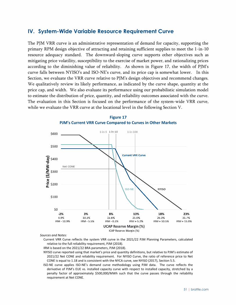
51 | brattle.com

IV. System-Wide Variable Resource Requirement Curve

The PJM VRR curve is an administrative representation of demand for capacity, supporting the

primary RPM design objective of attracting and retaining sufficient supplies to meet the 1-in-10

resource adequacy standard. The downward-sloping curve supports other objectives such as

mitigating price volatility, susceptibility to the exercise of market power, and rationalizing prices

according to the diminishing value of reliability. As shown in Figure 17, the width of PJM’s

curve falls between NYISO’s and ISO-NE’s curve, and its price cap is somewhat lower. In this

Section, we evaluate the VRR curve relative to PJM’s design objectives and recommend changes.

We qualitatively review its likely performance, as indicated by the curve shape, quantity at the

price cap, and width. We also evaluate its performance using our probabilistic simulation model

to estimate the distribution of price, quantity, and reliability outcomes associated with the curve.

The evaluation in this Section is focused on the performance of the system-wide VRR curve,

while we evaluate the VRR curve at the locational level in the following Section V.

Figure 17 PJM’s Current VRR Curve Compared to Curves in Other Markets

Sources and Notes:

Current VRR Curve reflects the system VRR curve in the 2021/22 PJM Planning Parameters, calculated relative to the full reliability requirement, PJM (2018).

IRM is based on the 2021/22 BRA parameters, PJM (2018). NYISO curve reported using that market’s price and quantity definitions, but relative to PJM’s estimate of

2021/22 Net CONE and reliability requirement. For NYISO Curve, the ratio of reference price to Net CONE is equal to 1.18 and is consistent with the NYCA curve, see NYISO (2017), Section 5.5.

ISO-NE curve applies ISO-NE’s demand curve methodology using PJM data. The curve reflects the derivative of PJM’s EUE vs. installed capacity curve with respect to installed capacity, stretched by a penalty factor of approximately $500,000/MWh such that the curve passes through the reliability requirement at Net CONE.

52 | brattle.com

Two changes in the market since our last review require careful attention in re-assessing the

VRR curve. First, as discussed in Section III.C, the introduction of Capacity Performance has

increased the risk of taking on a capacity obligation and has made the supply curve more

gradually sloping. In Section IV.C, we re-assess the VRR curve accounting for this effect, as well

as an updated view of supply and demand in the market. The review in Section IV.C focuses on

the change in VRR curve performance due to Capacity Performance and does not reflect the

impact of revised Net CONE values.

Second, and more importantly, the decrease in Net CONE since the last auction means that the

existing VRR curve must be scaled downward. In Section IV.D, we evaluate the performance of

several alternative curves using revised Net CONE values. We show that continuing to set the

VRR curve prices based on CT Net CONE when low-net-cost CCs are actually entering the

market can be expected to attract 5% excess capacity above the resource adequacy target in

equilibrium, at significant cost to customers. We recommend that PJM consider adopting a CC

reference resource and left-shifting the curve by 1%. This would lower customer costs while still

delivering better reliability than the curve PJM filed in 2014. We also show even more tightened

curves for PJM’s consideration.

A. SYSTEM-WIDE DESIGN OBJECTIVES

The primary design objective of the system-wide VRR curve is to procure enough resources to

maintain resource adequacy, including merchant entry when needed. This objective must be

fulfilled while aiming to avoid excessive price volatility and susceptibility to market power

abuse. These objectives can be at odds, with a vertical curve providing greater assurance of

procuring the target quantity, but producing prices that are maximally sensitive to small shifts in

supply and demand; in the other extreme, a horizontal curve provides total certainty in price but

provides no certainty in the quantity that will be procured or consequently in realized reliability

levels. Tradeoffs between quantity uncertainty and price uncertainty reflect the classic “prices

vs. quantities” problem in regulatory economics.60

In order to inform these tradeoffs and determine whether the VRR curve provides a satisfactory

balance, it is helpful to sharpen the definition of both the quantity-related and price-related

objectives. As we discussed in our 2014 Review, we have established the following specifications

in collaboration with PJM staff, consistent with PJM’s Tariff, practices, and prior statements:

Resource Adequacy (Quantities). Recognizing that procurement can be increased by

shifting the curve up or to the right, but cleared quantities will vary as supply and

demand conditions shift, our analysis assumes the VRR curve should meet the following

objectives:

60 See Weitzman (1974).

53 | brattle.com

– The expected LOLE should be 0.1 events per year. This does not mean the LOLE will

be 0.1 in every year, but that it can be expected to achieve the 1-event-in-10 years

LOLE target on average. We will continue to maintain this interpretation of the

reliability standard for the purposes of our assessment, even though we acknowledge

that the current VRR Curve has been right-shifted with the explicit purpose of

enhancing reliability.61

– Very low reserve margin outcomes should be realized from RPM auctions very

infrequently. For example, there should be a relatively small probability of clearing

less than “IRM – 1%,” the quantity at which PJM’s Tariff stipulates that a Reliability

Backstop Auction would occur under certain conditions.62

– The curve should meet these objectives in expectation and remain robust under a

range of future market conditions, changes in administrative parameters and

administrative estimation errors. However, considering that future VRR curve

reviews and CONE studies can adjust for major changes, it is unnecessary to

substantially over-procure on an expected average basis just to ensure meeting these

objectives under all conceivable future scenarios, as that would incur excess costs.

Prices. Consistent with relying on merchant entry, prices can be expected to equal Net

CONE on a long-run average basis (no matter what the shape of the VRR curve). But

prices will vary as supply and demand conditions shift, depending on the elasticity of the

supply and VRR curves. To support a well-functioning market, the VRR curve should

meet the following price-volatility-related objectives:

– The curve should achieve low price volatility, to the extent possible given other

design objectives. That means reducing the impact from small variations in supply

and demand, including administrative parameters, rule changes, lumpy investment

decisions, demand forecast changes, and transmission parameters.

– To mitigate susceptibility to the exercise of market power, small changes in supply

should not be allowed to produce large changes in price. Mitigating susceptibility to

market power and price volatility are both served by adopting a flatter VRR curve.

Relatedly, a VRR curve with a moderate price cap that limits the price impact of

withholding can address concerns about market power.

61 Following our 2014 Review, PJM filed a VRR curve that was 1% right-shifted relative to Brattle’s

recommended curve. Based on our modeling, PJM’s recommended curve would achieve an average

LOLE of 0.06 events/year and was associated with customer costs approximately 1% higher than

Brattle’s recommended curve. PJM chose this curve on the basis that short-term supply uncertainty in

the market might exceed what we accounted for in our simulation model due to a variety of policy

and market factors. See paragraph 25 of Federal Energy Regulatory Commission (2014).

62 Specifically, if the BRA clears a quantity less than IRM-1% for three consecutive years. See PJM

(2017h), Section 16.3.

54 | brattle.com

– However, price volatility should not be over-mitigated. Prices should be allowed to

vary sufficiently to reflect year-to-year changes in market conditions. It is preferred

for prices to rise increasingly steeply as reserve margins decrease in order to provide a

stronger price signal when needed to avoid very low reliability outcomes. Such a

convex VRR shape would also make prices more proportional to the marginal

reliability value, a desirable attribute for a “demand curve” for resource adequacy.63

– As noted above, the VRR curve needs a price cap, but it is important that the price

cap binds infrequently, to prevent prices from departing too substantially from supply

fundamentals.

Other Design Objectives. The VRR curve forms the basis for a multi-billion dollar

market, and yet it is an administratively-determined construct. To support a well-

functioning market for resource adequacy in which investors and other decision-makers

can expect continuity and develop a long-term view, this administrative construct should

be as rational, stable, and transparent as possible.

– The curve can be deemed “rational” if it consistently meets the design objectives

outlined above, with well-reasoned and balanced choices about tradeoffs among

objectives.

– To provide stability, the curve (and RPM as a whole) should have stable market rules

and administrative parameters, although adjustments may be necessary to

accommodate changes in market and system conditions.

– To support stability and transparency, the VRR curve should be simple in its

definition and in how parameters are updated over time. This can avoid stakeholder

contentiousness and litigation, which would increase regulatory risk for investors.

Several of these design objectives are difficult to satisfy simultaneously, and in many cases we

must weigh tradeoffs among competing design objectives. For example, capacity markets can

produce structurally volatile capacity prices due to steep supply and demand curves, meaning

that relatively small changes in supply or demand can cause large changes in price. Introducing a

sloped demand curve mitigates some of this price volatility, with flatter curves resulting in more

stable capacity prices. However, a very flat demand curve will introduce greater quantity

uncertainty and greater risk of low-reliability outcomes.

We evaluate the curve against the primary RPM design objective of achieving 1-in-10 LOLE on

average over many years. While we and others have separately evaluated the 1-in-10 standard

63 Since the VRR curve is designed to meet the engineering-based standard of 0.1 LOLE rather than an

economics-based reserve margin, the curve can only be designed to be proportional to marginal

reliability value rather than equal to the marginal economic value.

55 | brattle.com

itself from reliability and economic perspectives, this is not within the scope of our present

analysis.64

B. QUALITATIVE REVIEW OF THE CURRENT SYSTEM CURVE

Subsequent to our last review, PJM adopted a VRR curve consistent with the right-shifted

convex curve we analyzed in that study. Under the assumptions in that study, the adopted curve

was broadly consistent with PJM’s design objectives, though the curve procured more supply

than necessary to meet PJM’s 1-in-10 LOLE requirement on average. PJM determined that the

right-shifted curve’s reduced risk of low-reliability events and its improved robustness to adverse

conditions (e.g., larger than expected fluctuations in net supply, administrative under-estimation

of Net CONE) were worth the relatively small increase in procurement costs relative to our

recommended convex curve.65

While PJM’s current VRR curve performed well under the assumptions of our 2014 Review, it is

very likely to attract too much investment under current market conditions. The current curve

is based on our 2014 analysis, where we assumed entry occurs at a price approximately 2.5 times

higher than our current estimate of CC Net CONE.66 With the market entry price substantially

lower, the current demand curve is likely to attract more supply than is necessary to meet the 1-

in-10 standard in equilibrium. To better align the VRR curve with PJM’s resource adequacy

objectives, the curve could be stretched downwards and shifted to the left, as discussed below.

1. Downward-Sloping, Convex Shape

PJM’s VRR curve has a downward-sloping shape to the right of point “a” as described in Section

I.C above. This overall shape is consistent with PJM’s design objectives, with higher prices when

the system has less supply and lower prices when the system has more supply. This price and

quantity relationship should attract new capacity investments when the system is short on

supply, and postpone such investments when the system is long. The downward-sloping shape

of the curve will also help mitigate price volatility and the exercise of market power, consistent

with the design objectives.

The downward-sloping portion of PJM’s curve has a convex shape (i.e., curving away from the

intersection of the x- and y-axis), with a steeper slope at quantities near the requirement and a

flatter slope at higher quantities. A convex curve has the theoretical advantage of being

consistent with the incremental reliability and economic value of capacity, as illustrated in

Figure 18. The figure shows the VRR curve superimposed over the marginal avoided expected

64 For example, see Pfeifenberger (2013).

65 See p. 19 of PJM’s Filing Letter following the 2014 Review, PJM (2014f).

66 While based on the results of our analysis, PJM right-shifted our recommended curve by 1% to

develop the current VRR curve, leading to equilibrium supply above the level needed to achieve 1-in-

10 LOLE under the Net CONE value used in the 2014 Review.

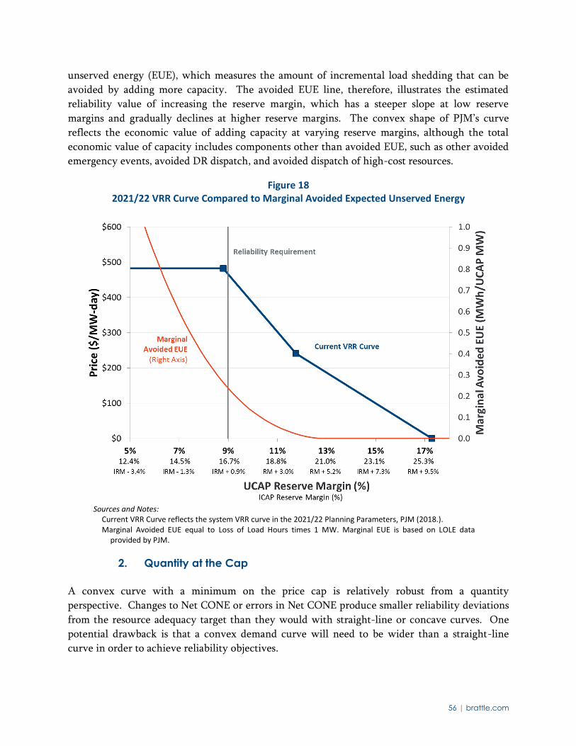
56 | brattle.com

unserved energy (EUE), which measures the amount of incremental load shedding that can be

avoided by adding more capacity. The avoided EUE line, therefore, illustrates the estimated

reliability value of increasing the reserve margin, which has a steeper slope at low reserve

margins and gradually declines at higher reserve margins. The convex shape of PJM’s curve

reflects the economic value of adding capacity at varying reserve margins, although the total

economic value of capacity includes components other than avoided EUE, such as other avoided

emergency events, avoided DR dispatch, and avoided dispatch of high-cost resources.

Figure 18 2021/22 VRR Curve Compared to Marginal Avoided Expected Unserved Energy

Sources and Notes:

Current VRR Curve reflects the system VRR curve in the 2021/22 Planning Parameters, PJM (2018.). Marginal Avoided EUE equal to Loss of Load Hours times 1 MW. Marginal EUE is based on LOLE data

provided by PJM.

2. Quantity at the Cap

A convex curve with a minimum on the price cap is relatively robust from a quantity

perspective. Changes to Net CONE or errors in Net CONE produce smaller reliability deviations

from the resource adequacy target than they would with straight-line or concave curves. One

potential drawback is that a convex demand curve will need to be wider than a straight-line

curve in order to achieve reliability objectives.

57 | brattle.com

The curve can be evaluated in terms of its reliability implications at varying reserve margins by

comparing the VRR curve to system LOLE at varying reserve margins. The most important

region of the curve from a reliability perspective is the high-priced region at reserve margins

below the 1-in-10 resource adequacy requirement. This is because LOLE and other reliability

metrics increase very quickly at low reserve margins, with small deviations below the

requirement having a disproportionately large impact in degrading reliability while similarly-

sized increases above the requirement result in relatively modest reliability improvements. For

example, increasing the reserve margin from IRM to IRM+2% changes LOLE from 0.10 to 0.036

events per year, while decreasing the reserve margin to IRM-2% changes LOLE from 0.10 to 0.24

events per year. A two percentage point decrease of reserve margin thus has an impact on

reliability that is more than twice as large as the impact of a two percentage point increase, and

this asymmetry is even greater for larger deviations.

PJM’s quantity at the cap is well to the right of its administrative reliability backstop threshold.

PJM’s Reliability Backstop provisions state that PJM must conduct a backstop procurement if the

BRA clears below a quantity of IRM-1% for three consecutive years.67 This IRM-1% threshold

corresponds to a reliability index of 1-in-6.5, whereas point “a” corresponds to a reliability index

of 1-in-9, as summarized in Table 7. This design preserves investment incentives by ensuring

that PJM procures all available resources at the price cap before triggering out-of-market

procurement. While the quantity at the cap should fall to the right of the Reliability Backstop to

avoid suppressing investment, this consideration does not require the quantity at the cap to be so

far to the right.

Table 7 Reliability at VRR Curve Quantity Points and Backstop Trigger

Sources and Notes:

Loss of Load Event (LOLE) shows the corresponding reliability for each quantity outcome shown, based on an exponential fit of LOLE and quantity as a percentage of reliability requirement. Reliability Index is the reciprocal of LOLE. Reliability data provided by PJM.

67 See Section OATT Attachment DD.16 PJM (2017h)

Quantity Point LOLE

Reliability

Index

(Ev/Yr) (1-in-X)

Backstop Trigger at IRM - 1% 0.15 1-in-6.5

Point "a" 0.11 1-in-9.0

Reliability Requirement at IRM 0.10 1-in-10.0

Point "b" 0.02 1-in-47.3

Point "c" 0.00 1-in-3577.2

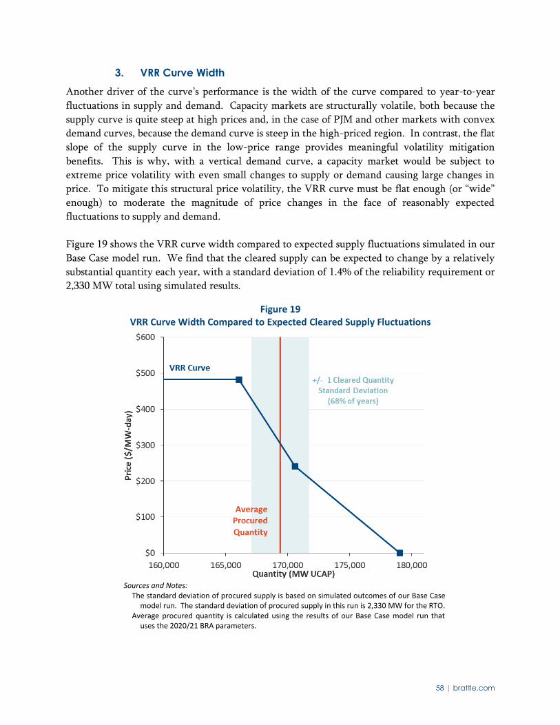
58 | brattle.com

3. VRR Curve Width

Another driver of the curve’s performance is the width of the curve compared to year-to-year

fluctuations in supply and demand. Capacity markets are structurally volatile, both because the

supply curve is quite steep at high prices and, in the case of PJM and other markets with convex

demand curves, because the demand curve is steep in the high-priced region. In contrast, the flat

slope of the supply curve in the low-price range provides meaningful volatility mitigation

benefits. This is why, with a vertical demand curve, a capacity market would be subject to

extreme price volatility with even small changes to supply or demand causing large changes in

price. To mitigate this structural price volatility, the VRR curve must be flat enough (or “wide”

enough) to moderate the magnitude of price changes in the face of reasonably expected

fluctuations to supply and demand.

Figure 19 shows the VRR curve width compared to expected supply fluctuations simulated in our

Base Case model run. We find that the cleared supply can be expected to change by a relatively

substantial quantity each year, with a standard deviation of 1.4% of the reliability requirement or

2,330 MW total using simulated results.

Figure 19 VRR Curve Width Compared to Expected Cleared Supply Fluctuations

Sources and Notes:

The standard deviation of procured supply is based on simulated outcomes of our Base Case model run. The standard deviation of procured supply in this run is 2,330 MW for the RTO.

Average procured quantity is calculated using the results of our Base Case model run that uses the 2020/21 BRA parameters.

59 | brattle.com

These year-to-year changes in cleared supply are relatively large compared to the width of the

VRR curve. As Figure 19 shows, if starting at the average cleared quantity from our reliability

modeling, losing one standard deviation of cleared supply would increase prices to near the cap

by a delta of about $115/MW-day or 38% of Net CONE; while adding one standard deviation of

net supply would decrease prices by about $87/MW-day or 30% of Net CONE. The consequence

of these relatively large deviations in cleared supply, combined with PJM’s current and past VRR

curves, is that RPM has produced relatively volatile price outcomes.

The magnitude of expected shifts to cleared supply has important implications for reliability. For

example, if prices need to be at Net CONE on average in long-run equilibrium, then assuming a

normal distribution in cleared supply fluctuations, we would expect quantities at IRM-1%

(reliability index 1-in-6.5) approximately once every 14 years and at IRM-3% (reliability index

1-in-2.6) approximately once every 42 years. However, supply fluctuations have not historically

resulted in low realized reserve margins, largely because RPM has been maintaining an average

reserve margin well in excess of the long-run equilibrium quantity.

C. SIMULATED PERFORMANCE WITH PRIOR NET CONE AND MARKET ENTRY PRICE

We use the probabilistic modeling approach described in Section III to evaluate VRR curve

performance. In order to first isolate the impact of Capacity Performance and allow for

comparison with the results of our 2014 Review, this section retains the same assumption as the

prior review: that the market entry price (i.e., the price at which developers are willing to enter

the market, or the true cost of entry) and the administrative Net CONE value used to define the

VRR curve are both equal to the parameter from the most recent auction.68 We estimate the

distribution of system-level price, quantity, and reliability outcomes that PJM’s VRR curve will

achieve given Capacity Performance and expected fluctuations in supply, demand, and

transmission.69 We then test the sensitivity of the curve’s performance to different assumptions

about the fluctuation sizes and the impact of Capacity Performance on supply offer prices.

Finally, we compare simulated performance of the VRR curve to alternative curve shapes and re-

examine the 1% right-shift adopted in the prior review.

We will separately address in Section IV.D the implications of recent reductions in the market

entry price. Our two-stage analytical approach allows us to show that (1) Capacity Performance

68 The prior review assumed the market entry price and administrative RTO Net CONE were $331/MW-

day, taken from the 2016/17 BRA parameters. The new simulations in this section assume $293/MW-

day, taken from the 2020/21 BRA parameters. However, the specific value does not significantly

affect simulated reliability. What does matter is the assumption that the administrative value used to

set prices in the VRR curve are equal to the true value developers need to earn in order to invest.

69 Our analysis in this and the following section uses updated supply, demand, and transmission

parameters reflecting the current state of the system. However, because these parameters did not

change substantially from our 2014 Review, they are not a major driver of our results.

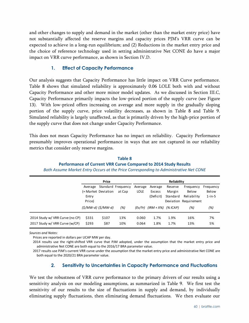
60 | brattle.com

and other changes to supply and demand in the market (other than the market entry price) have

not substantially affected the reserve margins and capacity prices PJM’s VRR curve can be

expected to achieve in a long-run equilibrium; and (2) Reductions in the market entry price and

the choice of reference technology used in setting administrative Net CONE do have a major

impact on VRR curve performance, as shown in Section IV.D.

1. Effect of Capacity Performance

Our analysis suggests that Capacity Performance has little impact on VRR Curve performance.

Table 8 shows that simulated reliability is approximately 0.06 LOLE both with and without

Capacity Performance and other more minor model updates. As we discussed in Section III.C,

Capacity Performance primarily impacts the low-priced portion of the supply curve (see Figure

13). With low-priced offers increasing on average and more supply in the gradually sloping

portion of the supply curve, price volatility decreases, as shown in Table 8 and Table 9.

Simulated reliability is largely unaffected, as that is primarily driven by the high-price portion of

the supply curve that does not change under Capacity Performance.

This does not mean Capacity Performance has no impact on reliability. Capacity Performance

presumably improves operational performance in ways that are not captured in our reliability

metrics that consider only reserve margins.

Table 8 Performance of Current VRR Curve Compared to 2014 Study Results

Both Assume Market Entry Occurs at the Price Corresponding to Administrative Net CONE

Sources and Notes:

Prices are reported in dollars per UCAP MW per day. 2014 results use the right-shifted VRR curve that PJM adopted, under the assumption that the market entry price and

administrative Net CONE are both equal to the 2016/17 BRA parameter value. 2017 results use PJM’s current VRR curve under the assumption that the market entry price and administrative Net CONE are

both equal to the 2020/21 BRA parameter value.

2. Sensitivity to Uncertainties in Capacity Performance and Fluctuations

We test the robustness of VRR curve performance to the primary drivers of our results using a

sensitivity analysis on our modeling assumptions, as summarized in Table 9. We first test the

sensitivity of our results to the size of fluctuations in supply and demand, by individually

eliminating supply fluctuations, then eliminating demand fluctuations. We then evaluate our

Price Reliability

Average

(= Market

Entry

Price)

Standard

Deviation

Frequency

at Cap

Average

LOLE

Average

Excess

(Deficit)

Reserve

Margin

Standard

Deviation

Frequency

Below

Reliability

Requirement

Frequency

Below

1-in-5

($/MW-d) ($/MW-d) (%) (Ev/Yr) (IRM + X%) (% ICAP) (%) (%)

2014 Study w/ VRR Curve (no CP) $331 $107 13% 0.060 1.7% 1.9% 16% 7%

2017 Study w/ VRR Curve (w/CP) $293 $87 10% 0.064 1.8% 1.7% 13% 5%

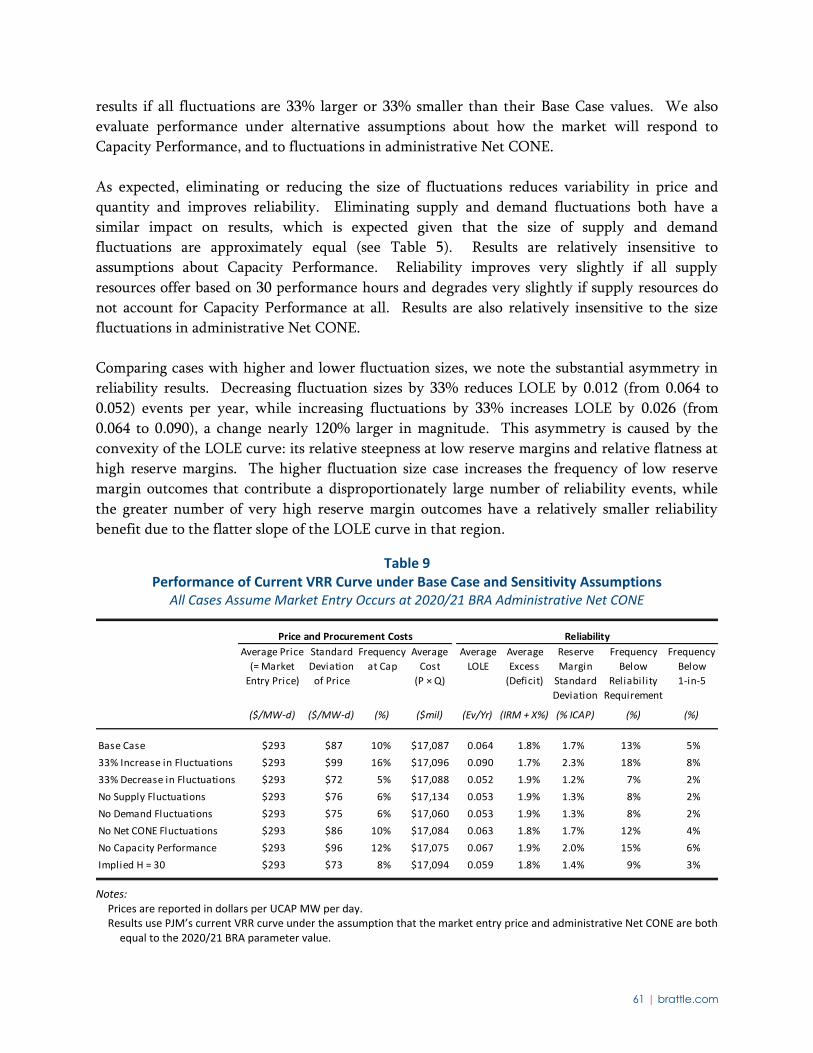
61 | brattle.com

results if all fluctuations are 33% larger or 33% smaller than their Base Case values. We also

evaluate performance under alternative assumptions about how the market will respond to

Capacity Performance, and to fluctuations in administrative Net CONE.

As expected, eliminating or reducing the size of fluctuations reduces variability in price and

quantity and improves reliability. Eliminating supply and demand fluctuations both have a

similar impact on results, which is expected given that the size of supply and demand

fluctuations are approximately equal (see Table 5). Results are relatively insensitive to

assumptions about Capacity Performance. Reliability improves very slightly if all supply

resources offer based on 30 performance hours and degrades very slightly if supply resources do

not account for Capacity Performance at all. Results are also relatively insensitive to the size

fluctuations in administrative Net CONE.

Comparing cases with higher and lower fluctuation sizes, we note the substantial asymmetry in

reliability results. Decreasing fluctuation sizes by 33% reduces LOLE by 0.012 (from 0.064 to

0.052) events per year, while increasing fluctuations by 33% increases LOLE by 0.026 (from

0.064 to 0.090), a change nearly 120% larger in magnitude. This asymmetry is caused by the

convexity of the LOLE curve: its relative steepness at low reserve margins and relative flatness at

high reserve margins. The higher fluctuation size case increases the frequency of low reserve

margin outcomes that contribute a disproportionately large number of reliability events, while

the greater number of very high reserve margin outcomes have a relatively smaller reliability

benefit due to the flatter slope of the LOLE curve in that region.

Table 9 Performance of Current VRR Curve under Base Case and Sensitivity Assumptions

All Cases Assume Market Entry Occurs at 2020/21 BRA Administrative Net CONE

Notes:

Prices are reported in dollars per UCAP MW per day. Results use PJM’s current VRR curve under the assumption that the market entry price and administrative Net CONE are both

equal to the 2020/21 BRA parameter value.

Price and Procurement Costs Reliability

Average Price

(= Market

Entry Price)

Standard

Deviation

of Price

Frequency

at Cap

Average

Cost

(P × Q)

Average

LOLE

Average

Excess

(Deficit)

Reserve

Margin

Standard

Deviation

Frequency

Below

Reliability

Requirement

Frequency

Below

1-in-5

($/MW-d) ($/MW-d) (%) ($mil) (Ev/Yr) (IRM + X%) (% ICAP) (%) (%)

Base Case $293 $87 10% $17,087 0.064 1.8% 1.7% 13% 5%

33% Increase in Fluctuations $293 $99 16% $17,096 0.090 1.7% 2.3% 18% 8%

33% Decrease in Fluctuations $293 $72 5% $17,088 0.052 1.9% 1.2% 7% 2%

No Supply Fluctuations $293 $76 6% $17,134 0.053 1.9% 1.3% 8% 2%

No Demand Fluctuations $293 $75 6% $17,060 0.053 1.9% 1.3% 8% 2%

No Net CONE Fluctuations $293 $86 10% $17,084 0.063 1.8% 1.7% 12% 4%

No Capacity Performance $293 $96 12% $17,075 0.067 1.9% 2.0% 15% 6%

Implied H = 30 $293 $73 8% $17,094 0.059 1.8% 1.4% 9% 3%

62 | brattle.com

3. Re-Evaluation of the Left-Shift of the VRR Curve

In 2014, PJM filed a 1% right-shifted curve relative to our recommended curve on the basis that

the market was facing substantial uncertainty in supply in the coming years. PJM and the FERC

Order cited several drivers of this uncertainty: large scale generation retirements due to the

Mercury and Air Toxics Standards, low-priced shale gas, increasing efficiency of gas combined-

cycle technology, the D.C. Circuit court’s vacatur of FERC’s Order 745, and the implementation

of the EPA’s Clean Power Plan.70 Due to these considerations, PJM placed more weight on the

risk of very low reliability events and on our “stress” cases involving high supply uncertainty and

administrative under-estimation of Net CONE. PJM concluded that a 1% right-shifted curve

would help it ride through any potential supply disruptions, while acknowledging that it might

lead to reliability better than 1-in-10 in the long-run average.

Most of the reasons for right-shifting the VRR curve that PJM cited in its 2014 filing are no

longer applicable. While we acknowledge the ongoing potential for retirement by plants not

covering their fixed costs, these economic retirements do not pose the same resource adequacy

challenge as the risk of simultaneous large-scale retirements under MATS. PJM’s market has

demonstrated its ability to manage economic retirements by attracting new capacity or

incentivizing incumbents to stay online as the market tightens. As a result, we would

recommend shifting the VRR curve back to the left, even if no changes to the market entry price

had occurred. Table 10 compares the performance of PJM’s current curve to a 1% left-shifted

curve under the assumption that the market entry price and administrative Net CONE both

equal the 2020/21 BRA parameter. The left-shifted curve achieves average LOLE of

approximately the 1-in-10 standard. Customer costs decrease by approximately $150 million per

year, or 1% of the total. The frequency of low reliability events (below 1-in-5) increases slightly,

but such events would still be rare.

70 See paragraph 25 of Federal Energy Regulatory Commission, 2014xa.

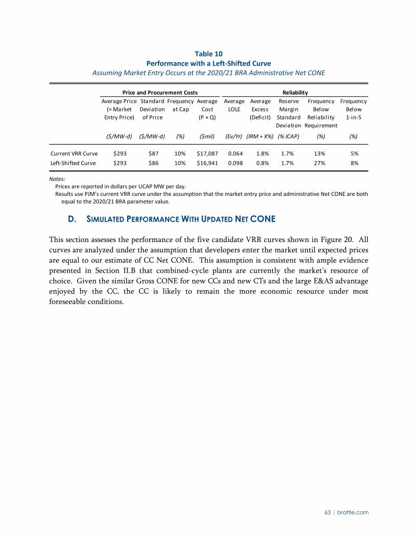
63 | brattle.com

Table 10 Performance with a Left-Shifted Curve

Assuming Market Entry Occurs at the 2020/21 BRA Administrative Net CONE

Notes:

Prices are reported in dollars per UCAP MW per day. Results use PJM’s current VRR curve under the assumption that the market entry price and administrative Net CONE are both

equal to the 2020/21 BRA parameter value.

D. SIMULATED PERFORMANCE WITH UPDATED NET CONE

This section assesses the performance of the five candidate VRR curves shown in Figure 20. All

curves are analyzed under the assumption that developers enter the market until expected prices

are equal to our estimate of CC Net CONE. This assumption is consistent with ample evidence

presented in Section II.B that combined-cycle plants are currently the market’s resource of

choice. Given the similar Gross CONE for new CCs and new CTs and the large E&AS advantage

enjoyed by the CC, the CC is likely to remain the more economic resource under most

foreseeable conditions.


Average Price

(= Market

Entry Price)

Standard

Deviation

of Price

Frequency

at Cap

Average

Cost

(P × Q)

Average

LOLE

Average

Excess

(Deficit)

Reserve

Margin

Standard

Deviation

Frequency

Below

Reliability

Requirement

Frequency

Below

1-in-5

($/MW-d) ($/MW-d) (%) ($mil) (Ev/Yr) (IRM + X%) (% ICAP) (%) (%)

Current VRR Curve $293 $87 10% $17,087 0.064 1.8% 1.7% 13% 5%

Left-Shifted Curve $293 $86 10% $16,941 0.098 0.8% 1.7% 27% 8%

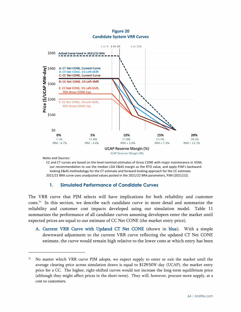
64 | brattle.com

Figure 20 Candidate System VRR Curves

Notes and Sources:

CC and CT curves are based on the level-nominal estimates of Gross CONE with major maintenance in VOM, our recommendation to use the median LDA E&AS margin as the RTO value, and apply PJM’s backward-looking E&AS methodology for the CT estimate and forward-looking approach for the CC estimate.

2021/22 BRA curve uses unadjusted values posted in the 2021/22 BRA parameters, PJM (2021/22).

1. Simulated Performance of Candidate Curves

The VRR curve that PJM selects will have implications for both reliability and customer

costs.71 In this section, we describe each candidate curve in more detail and summarize the

reliability and customer cost impacts developed using our simulation model. Table 11

summarizes the performance of all candidate curves assuming developers enter the market until

expected prices are equal to our estimate of CC Net CONE (the market entry price).

A. Current VRR Curve with Updated CT Net CONE (shown in blue). With a simple

downward adjustment to the current VRR curve reflecting the updated CT Net CONE

estimate, the curve would remain high relative to the lower costs at which entry has been

71 No matter which VRR curve PJM adopts, we expect supply to enter or exit the market until the

average clearing price across simulation draws is equal to $129/MW-day (UCAP), the market entry

price for a CC. The higher, right-shifted curves would not increase the long-term equilibrium price

(although they might affect prices in the short-term). They will, however, procure more supply, at a

cost to customers.

65 | brattle.com

occurring. This procures substantially more supply than needed to meet the 1-in-10

LOLE standard. Simulated long-run reserve margins are 4.3% above target on average

and limit expected annual loss-of-load events (LOLE) to 0.011—approximately ten times

more reliable than PJM’s resource adequacy standard of 0.1 events per year.

B. 1% Left-Shifted Curve with CT Net CONE (shown in light blue). Relative to curve A,

curve B would reduce the supply in the market by 1% and thus reduce annual

procurement costs by $74 million, and yet still achieve LOLE of 0.023, more than four

times better than the standard. The 1% left-shift undoes the right-shift that PJM

implemented four years ago. We recommend undoing the prior shift because most of the

regulatory and market conditions that helped justify the right-shift of the demand curve

have now been resolved.72

C. Current VRR Curve with CC Net CONE (shown in dark red). Similar to curve A, but this

curve applies a greater downward adjustment to align the curve with the prices at which

new capacity is available. However, the high CC E&AS offset triggers the alternative

price cap provision of PJM’s tariff, under which the cap is raised to Gross CONE when

Net CONE falls below 2/3 of Gross CONE. The alternative price cap at Gross CONE lifts

the price cap to approximately 2.6 × Net CONE and stretches the left half of the curve

upward, supporting greater entry. Compared to curve A that reflects the CT Net CONE

estimate, this curve decreases excess capacity by 1.5%, reducing procurement costs by

$100 million. Expected reserve margins are still 2.8% above the resource adequacy target

and expected LOLE is 0.031, over three times better than the resource adequacy standard.

D. 1% Left-Shifted Curve with CC Net CONE (shown in medium red). Similar to curve C,

but left-shifted. The reliability performance of this curve is approximately 0.05 LOLE per

year, still exceeding the 0.1 LOLE target by a factor of nearly 2 on average and falling

below the IRM target in only 5% of all simulated years. Even if the true market entry

price were 20% higher than the CC Net CONE estimate that is used to anchor the VRR

curve, simulated LOLE would be 0.072. This curve results in annual capacity

procurement costs that are $96 million less than under the curve B and $71 million less

than under curve C.

72 We understand that PJM right-shifted the curve we had recommended based on simulations, in part

because of short-term drivers of supply uncertainty that may not have been fully captured in our

modeling at the time, including Mercury Air Toxics Standards retirements, low gas prices, EPA’s

Clean Power Plan, and the D.C. Circuit Court’s vacatur of FERC Order 745. Many of these challenges

are no longer a concern, and the market has demonstrated robust replacement of retiring resources.

While we acknowledge the ongoing potential for retirement by plants not covering their fixed costs,

these economic retirements do not pose the same resource adequacy challenge as the risk of

simultaneous large-scale retirements under MATS. PJM’s market has demonstrated its ability to

manage economic retirements by attracting new capacity or incentivizing incumbents to stay online

as the market tightens.

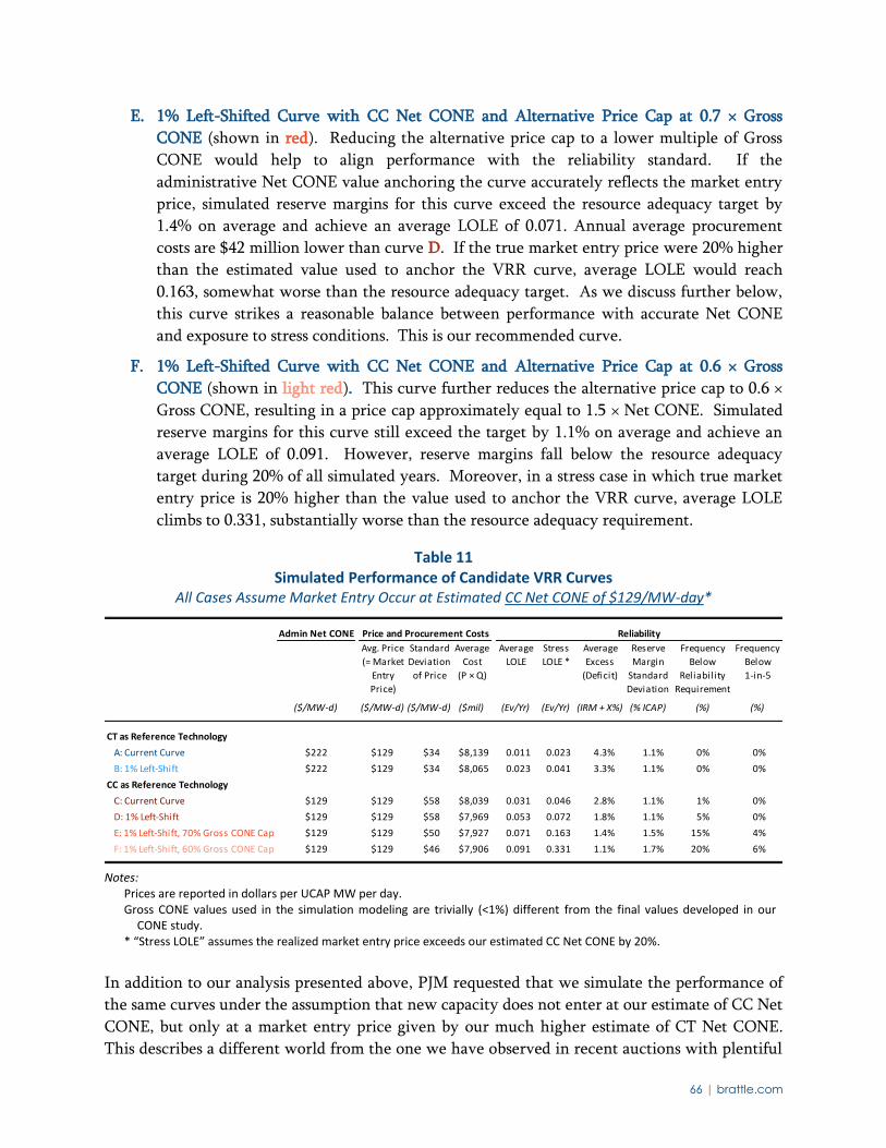
66 | brattle.com

E. 1% Left-Shifted Curve with CC Net CONE and Alternative Price Cap at 0.7 × Gross

CONE (shown in red). Reducing the alternative price cap to a lower multiple of Gross

CONE would help to align performance with the reliability standard. If the

administrative Net CONE value anchoring the curve accurately reflects the market entry

price, simulated reserve margins for this curve exceed the resource adequacy target by

1.4% on average and achieve an average LOLE of 0.071. Annual average procurement

costs are $42 million lower than curve D. If the true market entry price were 20% higher

than the estimated value used to anchor the VRR curve, average LOLE would reach

0.163, somewhat worse than the resource adequacy target. As we discuss further below,

this curve strikes a reasonable balance between performance with accurate Net CONE

and exposure to stress conditions. This is our recommended curve.

F. 1% Left-Shifted Curve with CC Net CONE and Alternative Price Cap at 0.6 × Gross

CONE (shown in light red). This curve further reduces the alternative price cap to 0.6 ×

Gross CONE, resulting in a price cap approximately equal to 1.5 × Net CONE. Simulated

reserve margins for this curve still exceed the target by 1.1% on average and achieve an

average LOLE of 0.091. However, reserve margins fall below the resource adequacy

target during 20% of all simulated years. Moreover, in a stress case in which true market

entry price is 20% higher than the value used to anchor the VRR curve, average LOLE

climbs to 0.331, substantially worse than the resource adequacy requirement.

Table 11 Simulated Performance of Candidate VRR Curves

All Cases Assume Market Entry Occur at Estimated CC Net CONE of $129/MW-day*

Notes:


CONE study. * “Stress LOLE” assumes the realized market entry price exceeds our estimated CC Net CONE by 20%.

In addition to our analysis presented above, PJM requested that we simulate the performance of

the same curves under the assumption that new capacity does not enter at our estimate of CC Net

CONE, but only at a market entry price given by our much higher estimate of CT Net CONE. This describes a different world from the one we have observed in recent auctions with plentiful


Avg. Price

(= Market

Entry

Price)

Standard

Deviation

of Price

Average

Cost

(P × Q)

Average

LOLE

Stress

LOLE *

Average

Excess

(Deficit)

Reserve

Margin

Standard

Deviation

Frequency

Below

Reliability

Requirement

Frequency

Below

1-in-5

($/MW-d) ($/MW-d) ($/MW-d) ($mil) (Ev/Yr) (Ev/Yr) (IRM + X%) (% ICAP) (%) (%)


A: Current Curve $222 $129 $34 $8,139 0.011 0.023 4.3% 1.1% 0% 0%

B: 1% Left-Shift $222 $129 $34 $8,065 0.023 0.041 3.3% 1.1% 0% 0%


C: Current Curve $129 $129 $58 $8,039 0.031 0.046 2.8% 1.1% 1% 0%

D: 1% Left-Shift $129 $129 $58 $7,969 0.053 0.072 1.8% 1.1% 5% 0%

E: 1% Left-Shift, 70% Gross CONE Cap $129 $129 $50 $7,927 0.071 0.163 1.4% 1.5% 15% 4%

F: 1% Left-Shift, 60% Gross CONE Cap $129 $129 $46 $7,906 0.091 0.331 1.1% 1.7% 20% 6%

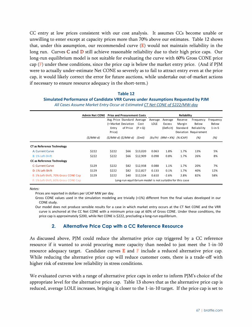
67 | brattle.com

CC entry at low prices consistent with our cost analysis. It assumes CCs become unable or

unwilling to enter except at capacity prices more than 70% above our estimates. Table 12 shows

that, under this assumption, our recommended curve (E) would not maintain reliability in the

long run. Curves C and D still achieve reasonable reliability due to their high price caps. Our

long-run equilibrium model is not suitable for evaluating the curve with 60% Gross CONE price

cap (F) under these conditions, since the price cap is below the market entry price. (And if PJM

were to actually under-estimate Net CONE so severely as to fail to attract entry even at the price

cap, it would likely correct the error for future auctions, while undertake out-of-market actions

if necessary to ensure resource adequacy in the short-term.)

Table 12 Simulated Performance of Candidate VRR Curves under Assumptions Requested by PJM

All Cases Assume Market Entry Occur at Estimated CT Net CONE of $222/MW-day

Notes:


CONE study. Our model does not produce sensible results for a case in which market entry occurs at the CT Net CONE and the VRR

curve is anchored at the CC Net CONE with a minimum price cap at 60% of Gross CONE. Under these conditions, the price cap is approximately $200, while Net CONE is $222, precluding a long-run equilibrium.

2. Alternative Price Cap with a CC Reference Resource

As discussed above, PJM could reduce the alternative price cap triggered by a CC reference

resource if it wanted to avoid procuring more capacity than needed to just meet the 1-in-10

resource adequacy target. Candidate curves E and F include a reduced alternative price cap.

While reducing the alternative price cap will reduce customer costs, there is a trade-off with

higher risk of extreme low reliability in stress conditions.

We evaluated curves with a range of alternative price caps in order to inform PJM’s choice of the

appropriate level for the alternative price cap. Table 13 shows that as the alternative price cap is

reduced, average LOLE increases, bringing it closer to the 1-in-10 target. If the price cap is set to


Avg. Price

(= Market

Entry

Price)

Standard

Deviation

of Price

Average

Cost

(P × Q)

Average

LOLE

Average

Excess

(Deficit)

Reserve

Margin

Standard

Deviation

Frequency

Below

Reliability

Requirement

Frequency

Below

1-in-5

($/MW-d) ($/MW-d) ($/MW-d) ($mil) (Ev/Yr) (IRM + X%) (% ICAP) (%) (%)


A: Current Curve $222 $222 $66 $13,020 0.063 1.8% 1.7% 13% 5%

B: 1% Left-Shift $222 $222 $66 $12,909 0.098 0.8% 1.7% 26% 8%


C: Current Curve $129 $222 $82 $12,938 0.088 1.1% 1.7% 20% 7%

D: 1% Left-Shift $129 $222 $82 $12,827 0.133 0.1% 1.7% 40% 12%

E: 1% Left-Shift, 70% Gross CONE Cap $129 $222 $40 $12,534 0.610 -2.6% 2.8% 82% 58%

F: 1% Left-Shift, 60% Gross CONE Cap Long-run equilibrium model is not suitable for this case

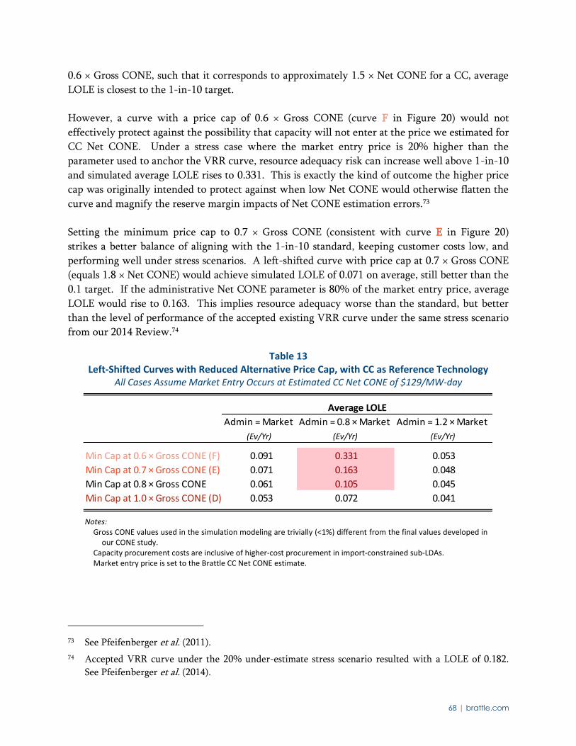
68 | brattle.com

0.6 × Gross CONE, such that it corresponds to approximately 1.5 × Net CONE for a CC, average

LOLE is closest to the 1-in-10 target.

However, a curve with a price cap of 0.6 × Gross CONE (curve F in Figure 20) would not

effectively protect against the possibility that capacity will not enter at the price we estimated for

CC Net CONE. Under a stress case where the market entry price is 20% higher than the

parameter used to anchor the VRR curve, resource adequacy risk can increase well above 1-in-10

and simulated average LOLE rises to 0.331. This is exactly the kind of outcome the higher price

cap was originally intended to protect against when low Net CONE would otherwise flatten the

curve and magnify the reserve margin impacts of Net CONE estimation errors.73

Setting the minimum price cap to 0.7 × Gross CONE (consistent with curve E in Figure 20)

strikes a better balance of aligning with the 1-in-10 standard, keeping customer costs low, and

performing well under stress scenarios. A left-shifted curve with price cap at 0.7 × Gross CONE

(equals 1.8 × Net CONE) would achieve simulated LOLE of 0.071 on average, still better than the

0.1 target. If the administrative Net CONE parameter is 80% of the market entry price, average

LOLE would rise to 0.163. This implies resource adequacy worse than the standard, but better

than the level of performance of the accepted existing VRR curve under the same stress scenario

from our 2014 Review.74

Table 13 Left-Shifted Curves with Reduced Alternative Price Cap, with CC as Reference Technology

All Cases Assume Market Entry Occurs at Estimated CC Net CONE of $129/MW-day

Notes:

Gross CONE values used in the simulation modeling are trivially (<1%) different from the final values developed in our CONE study.

Capacity procurement costs are inclusive of higher-cost procurement in import-constrained sub-LDAs. Market entry price is set to the Brattle CC Net CONE estimate.

73 See Pfeifenberger et al. (2011).

74 Accepted VRR curve under the 20% under-estimate stress scenario resulted with a LOLE of 0.182.

See Pfeifenberger et al. (2014).

Average LOLE

Admin = Market Admin = 0.8 × Market Admin = 1.2 × Market

(Ev/Yr) (Ev/Yr) (Ev/Yr)

Min Cap at 0.6 × Gross CONE (F) 0.091 0.331 0.053

Min Cap at 0.7 × Gross CONE (E) 0.071 0.163 0.048

Min Cap at 0.8 × Gross CONE 0.061 0.105 0.045

Min Cap at 1.0 × Gross CONE (D) 0.053 0.072 0.041

69 | brattle.com

E. SUMMARY AND RECOMMENDATIONS FOR THE SYSTEM-WIDE VRR CURVE

We conclude that maintaining the CT as the reference technology for anchoring the VRR curve

would procure more capacity than needed given the likely entry of CCs at a lower cost. To

better align the curve with the cost at which capacity is actually available and with PJM’s

objective to meet resource adequacy requirements cost-effectively, we recommend adopting CCs

as the reference technology. Furthermore, our simulations indicate that shifting the curve 1%

left and reducing the alternative price cap to 0.7 × Gross CONE (curve E) would better meet and

not exceed resource adequacy objectives. Simulated reliability slightly exceeds the 1-in-10

standard, with a reserve margin exceeding the target IRM 85% of the time, assuming

administrative Net CONE reflects the true price developers need to enter. If the true value were

20% higher than the value applied to the VRR curve, reliability would fall short of the

requirement but not nearly as much as with alternative curves with the lower cap; reliability

would exceed that of the accepted existing VRR curve under the same stress scenario from our

2014 Review.75,76 With $140 million lower annual average procurement costs than with the left-

shifted CT-based curve (curve B), this curve seems to represent a reasonable tradeoff between

cost and performance under adverse conditions. Curve E is therefore the VRR curve we

recommend.

Shifting from the current curve (dark blue dashed line) to our recommended curve (E) is a

substantial change that might raise concerns about market stability and reliability. It is true that

this change risks under-procuring capacity if our estimate of CC Net CONE is much lower than

the actual price at which developers will enter the next several auctions. However, this seems

unlikely based on our CONE study and recent history with robust entry at low prices. For

example, if this curve had been in place for the 2020/21 BRA, the auction would likely still have

cleared more than 3% above the IRM target.

However we see an argument that a CT-based curve would more strongly guarantee resource

adequacy under all conditions, at a cost that is modest when put in context. A $140 million

difference in procurement costs (compared to curve B) is less than 0.5% of PJM’s total annual

wholesale costs. Overall, PJM’s market-based resource adequacy construct appears to have saved

much more than that by attracting and retaining a wide range of resources at competitive market

prices well below the estimated cost of new plants.77

75 We also evaluated the impact of lowering the alternative price cap to 0.8 × Gross CONE, which

achieves expected LOLE of 0.061, and 0.105 in the “stress case.”

76 Accepted VRR curve under the 20% under-estimate stress scenario resulted with a LOLE of 0.182.

See Pfeifenberger et al. (2014).

77 See Pfeifenberger et al. (2008, 2011, and 2014).

70 | brattle.com

V. Locational Variable Resource Requirement Curves

Resource adequacy challenges in the Locational Deliverability Areas (LDAs) level are of a

different nature than for the system. The impact of fluctuations in transmission import limits

and supply can be large in percentage terms, which can substantially impact local reserve

margins. RPM’s pricing dynamics play a key role in supporting local resource adequacy. The

clearing price in the parent zone acts as a price floor for the LDA, with the LDA price-separating

above the parent only when import limits are binding. This dynamic tends to limit downside

price volatility in the LDA, attract local supply, and support reliability. However, LDAs with

significantly higher Net CONE than their parent areas will have to price separate more

frequently in order for average clearing prices to provide the Net CONE premium, and with

lower reliability in those instances.

Our analysis of VRR curves for the LDAs focuses on these dynamics, rather than the impact of

recent low market entry prices and the choice of reference technology. Our analysis of

locational performance simply assumes that administrative Net CONE and the market entry price

are equal to each other (using the 2020/21 BRA parameter, similar to Section IV.C). Starting

from this base assumption, we then explore the impact of potential future conditions with

different prices differences between LDAs and parent zones.

In the 2020/21 BRA parameters, most LDAs have market entry prices below their parents and

our simulated results show that LDAs easily meet the 1-in-25 reliability standard. However, we

caution that LDA market entry prices may not remain below parent levels in a long-run

equilibrium where increased entry reduces E&AS offsets and increases the costs that must be

recovered in the capacity market. We estimate that when the market entry price is 5% higher in

each LDA compared to its parent (and the administrative Net CONE parameter is also 5%

higher), five of the fourteen LDAs fail to meet the 1-in-25 standard. To address the greater risk

of locational reliability challenges, we recommend a higher price cap for the locational demand

curves at 1.7 × Net CONE. This results in a curve with a similar price cap to our recommended

system level curve (curve E in Figure ES-1), but without the 1% left-shift. We also recommend a

minimum LDA demand curve width at 25% of the Capacity Emergency Transfer Limit (CETL).

These two adjustments combined reduce the locational reliability risks and result in each of the

fourteen LDAs meeting the 1-in-25 LOLE target.

A. SUMMARY OF LOCATIONAL RELIABILITY REQUIREMENT

PJM’s local resource adequacy requirements are set based on a 1-in-25 or 0.04 conditional LOLE

standard. The locational standard reflects the total amount of local supply plus imports that

would be needed to meet 0.04 LOLE under the conditional assumption that imports are fully

available at the CETL import limit.78 Taken at face value, the local standard would appear to

78 See PJM (2017g), Section 2.2.

71 | brattle.com

suggest that an import-constrained LDA would be more reliable than the system as a whole, with

local load shed events only once every 25 years compared to once every 10 years at the system

level. This is not the case, however, because the local 1-in-25 reliability standard does not

include all of the reliability events that an LDA would be expected to experience (the LDA is also

subject to loss of load in the event of system-wide shortages). Instead, the local 1-in-25 is a

conditional LOLE standard, measuring local reliability events that would occur if the LDA could

always import up to the CETL limit (i.e., assuming no outages at the system level or parent LDA

level.)

An additional complexity in the local standard is that the realized reliability at the LDA level

depends on the level of overlap between the local outage events and the system-wide and parent

LDA outage events. For a first-level LDA, the realized LOLE could be as low as 0.10 or as high as

0.14, if the events occur at exactly the same time or at entirely different times from the system-

wide outage events. For a fourth-level LDA, realized LOLE could be as low as 0.1 or as high as

0.26 in the unlikely event that all outage events occur at different times, as well as in its parent

LDAs and RTO. Thus, the reliability standard as currently implemented could result in very

different LOLEs at different locations within PJM’s footprint, with the estimated reliability not

reported after considering this additive effect.

Beyond these potential discrepancies in LOLEs by LDA, there may be larger discrepancies in

realized reliability among LDAs based on the definition of LOLE itself. While LOLE is a widely-

used metric for determining reliability standards, it is relatively less meaningful than some

alternatives. Because LOLE counts only load shed events, but not their depth or duration, it will

treat a small, short event and a large, widespread event with equal importance. The metric may

also have very different meanings at different LDA levels, since the magnitude of outages is not

normalized by the LDA size. As we discussed in our 2014 Review, PJM could consider switching

to a locational reliability requirement based on Expected Unserved Energy to address this

shortcoming.

B. QUALITATIVE REVIEW OF LOCATIONAL CURVES

In this Section, we qualitatively evaluate the VRR curve as applied at the local level, to develop

intuition around the likely performance concerns and locational price efficiency, before

estimating its performance quantitatively in subsequent Sections. In developing this evaluation,

we: (1) review the design objectives at the local level, specifically the Net CONE parameters; and

(2) review the price cap and shape of the demand curves at the local level.

1. LDA Net CONE

In both our Base Case and with updated CC and CT Net CONE, some LDAs have lower Net

CONE than their parent zones. However, long-run average LDA Net CONE may not remain

72 | brattle.com

lower than parent Net CONE.79 If LDA Net CONE is temporarily lower than parent Net CONE,

the LDA would attract new supply because of the attractiveness of a more economic investment

opportunity (with lower Net CONE but equal or higher capacity prices). This additional supply

would tend to reduce local energy prices and possibly raise local gas prices, eroding the E&AS

margin in the LDA and ultimately increasing LDA Net CONE. Since capacity prices in the LDA

have a soft floor at the parent price, supply will likely continue to enter in the LDA until LDA

Net CONE reaches or exceeds parent Net CONE. If long-run average LDA Net CONE rises above

the parent Net CONE, PJM’s LDAs would remain import-constrained in the long-run

equilibrium. If instead the E&AS margin does not erode, lower Net CONE values could persist in

the long-run equilibrium. In this case, supply would continue to enter the LDA until it ceases to

be import constrained in the long-run equilibrium.

The case where LDAs have higher Net CONE than their parents is more important, since that is

the only case where the local VRR curve will impact price and quantity outcomes in the long

term. VRR curves should be designed to perform well in this case. Our locational simulated

performance in the remainder of this section focuses on cases where each LDA is import-

constrained, with a Net CONE higher than the parent LDA. In these cases, our results suggest

that having a higher price cap in the LDAs will improve reliability to meet 1-in-25 LOLE target.

2. Locational Curve Price Cap and Shape

Similar to the system-level comparison of reliability metrics and the VRR curve from Section

IV.B, we compare the local VRR curves to the LDA conditional LOLE curves as shown in Figure

21. We place particular emphasis on the shape of the curve at quantities below the reliability

requirement, and observe that prices will reach the cap before rapidly increasing LOLE resulting

in very low reliability outcomes. The LDA VRR curves have the same shape as PJM’s current

system VRR curve. Based on the current VRR curve, prices would reach the cap at conditional

LOLE values of approximately 0.042 to 0.045 (reliability index of 1-in-24 to 1-in-22, compared to

a standard of 1-in-25) depending on the LDA.

79 In our third triennial review, we recommended imposing a minimum on LDA Net CONE at the

parent level to mitigate the risk of underestimating locational Net CONE and reducing reliability. As

we noted in the previous analysis, many of the smaller LDAs lack a local CONE estimate and have a

small sample of new generation data points to inform Gross CONE and E&AS margins. It is therefore

more likely that Gross CONE estimates in those LDAs do not accurately represent local siting and

permitting costs and that Net CONE estimates may reflect inaccurate E&AS margins. As discussed

above, under-procurement in the smaller LDAs reduces reliability more severely than it would at the

system level. The FERC rejected PJM’s proposal in 2014, citing a lack of firm basis to support the

proposal. FERC stated “this [Net CONE floor at parent level] proposal could operate to disconnect

costs and/or revenues from the areas to which they can be attributed, particularly given that

generators in a congested area may receive higher energy market revenues than in uncongested areas,

thereby warranting a larger EAS Offset in the congested area.” See FERC (2014), Section V.E.4.

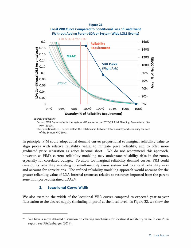
73 | brattle.com

Figure 21 Local VRR Curve Compared to Conditional Loss of Load Event

(Without Adding Parent-LDA or System-Wide LOLE Events)

Sources and Notes:

Current VRR Curve reflects the system VRR curve in the 2020/21 PJM Planning Parameters. See PJM (2017c).

The Conditional LOLE curves reflect the relationship between total quantity and reliability for each of the 14 non-RTO LDAs.

In principle, PJM could adopt zonal demand curves proportional to marginal reliability value to

align prices with relative reliability value, to mitigate price volatility, and to offer more

graduated price separation as zones become short. We do not recommend this approach,

however, as PJM’s current reliability modeling may understate reliability risks in the zones,

especially for correlated outages. To allow for marginal reliability demand curves, PJM could

develop its reliability modeling to simultaneously assess system and locational reliability risks

and account for correlations. The refined reliability modeling approach would account for the

greater reliability value of LDA-internal resources relative to resources imported from the parent

zone in import-constrained LDAs.80

3. Locational Curve Width

We also examine the width of the locational VRR curves compared to expected year-to-year

fluctuation to the cleared supply (including imports) at the local level. In Figure 22, we show the

80 We have a more detailed discussion on clearing mechanics for locational reliability value in our 2014

report, see Pfeifenberger (2014).

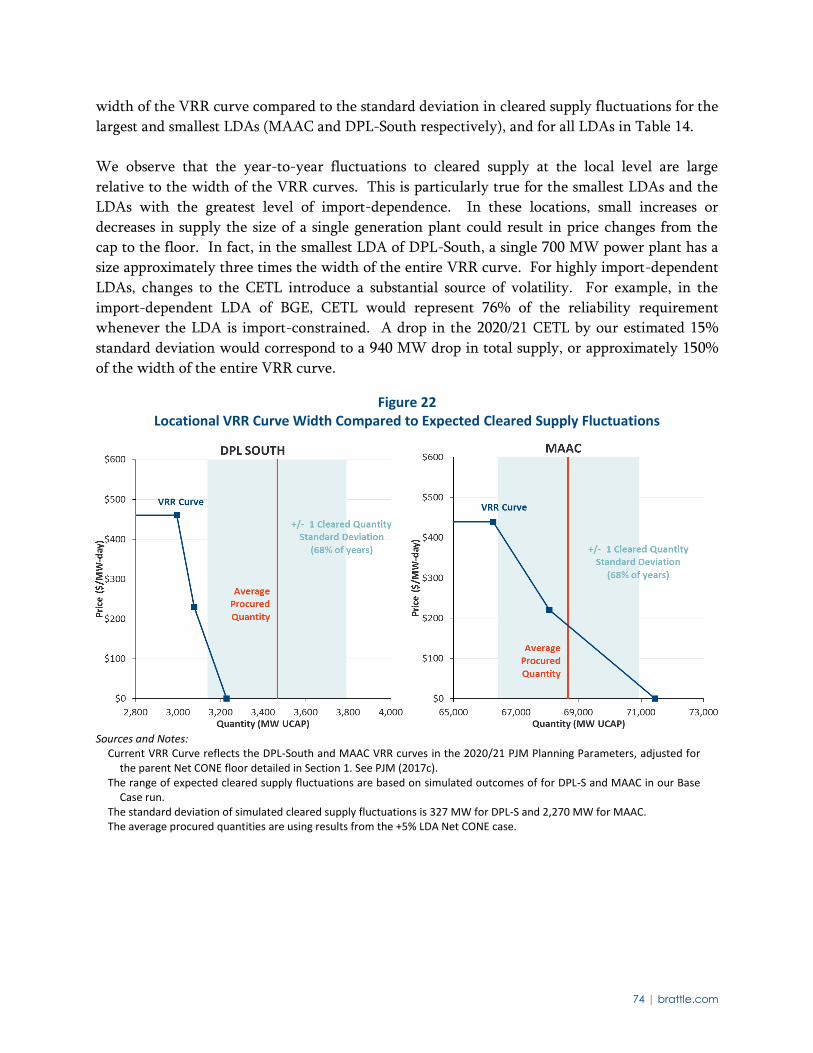
74 | brattle.com

width of the VRR curve compared to the standard deviation in cleared supply fluctuations for the

largest and smallest LDAs (MAAC and DPL-South respectively), and for all LDAs in Table 14.

We observe that the year-to-year fluctuations to cleared supply at the local level are large

relative to the width of the VRR curves. This is particularly true for the smallest LDAs and the

LDAs with the greatest level of import-dependence. In these locations, small increases or

decreases in supply the size of a single generation plant could result in price changes from the

cap to the floor. In fact, in the smallest LDA of DPL-South, a single 700 MW power plant has a

size approximately three times the width of the entire VRR curve. For highly import-dependent

LDAs, changes to the CETL introduce a substantial source of volatility. For example, in the

import-dependent LDA of BGE, CETL would represent 76% of the reliability requirement

whenever the LDA is import-constrained. A drop in the 2020/21 CETL by our estimated 15%

standard deviation would correspond to a 940 MW drop in total supply, or approximately 150%

of the width of the entire VRR curve.

Figure 22 Locational VRR Curve Width Compared to Expected Cleared Supply Fluctuations

Sources and Notes: Current VRR Curve reflects the DPL-South and MAAC VRR curves in the 2020/21 PJM Planning Parameters, adjusted for

the parent Net CONE floor detailed in Section 1. See PJM (2017c). The range of expected cleared supply fluctuations are based on simulated outcomes of for DPL-S and MAAC in our Base

Case run. The standard deviation of simulated cleared supply fluctuations is 327 MW for DPL-S and 2,270 MW for MAAC. The average procured quantities are using results from the +5% LDA Net CONE case.

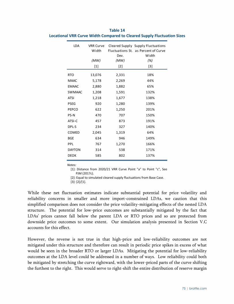
75 | brattle.com

Table 14 Locational VRR Curve Width Compared to Cleared Supply Fluctuation Sizes

Notes:

[1]: Distance from 2020/21 VRR Curve Point "a" to Point "c", See PJM (2017c).

[2]: Equal to simulated cleared supply fluctuations from Base Case. [3]: [2]/[1].

While these net fluctuation estimates indicate substantial potential for price volatility and

reliability concerns in smaller and more import-constrained LDAs, we caution that this

simplified comparison does not consider the price volatility-mitigating effects of the nested LDA

structure. The potential for low-price outcomes are substantially mitigated by the fact that

LDAs’ prices cannot fall below the parent LDA or RTO prices and so are protected from

downside price outcomes to some extent. Our simulation analysis presented in Section V.C

accounts for this effect.

However, the reverse is not true in that high-price and low-reliability outcomes are not

mitigated under this structure and therefore can result in periodic price spikes in excess of what

would be seen in the broader RTO or larger LDAs. Mitigating the potential for low-reliability

outcomes at the LDA level could be addressed in a number of ways. Low reliability could both

be mitigated by stretching the curve rightward, with the lower-priced parts of the curve shifting

the furthest to the right. This would serve to right-shift the entire distribution of reserve margin

LDA VRR Curve

Width

Cleared Supply

Fluctuations St.

Dev.

Supply Fluctuations

as Percent of Curve

Width

(MW) (MW) (%)

[1] [2] [3]

RTO 13,076 2,331 18%

MAAC 5,178 2,269 44%

EMAAC 2,880 1,882 65%

SWMAAC 1,208 1,591 132%

ATSI 1,218 1,677 138%

PSEG 920 1,280 139%

PEPCO 622 1,250 201%

PS-N 470 707 150%

ATSI-C 457 873 191%

DPL-S 234 327 140%

COMED 2,045 1,319 64%

BGE 634 946 149%

PPL 767 1,270 166%

DAYTON 314 538 171%

DEOK 585 802 137%

76 | brattle.com

outcomes. Alternatively, the price cap in the LDAs could be increased relative to the system

level in order to increase supply during shortage conditions.

Changes to the locational VRR curve are not the only way to address these concerns. Similar to

our 2014 Review, we recommend that PJM continue to review options for increasing the

predictability and stability of its administrative CETL estimates. Reducing volatility in this

parameter could substantially reduce the likelihood and magnitude of price spikes in LDAs.

However, we caution that approaches to reducing CETL volatility should be focused on reducing

volatility within the bands of administrative uncertainty, but should not prevent CETL from

changing with physical changes to the transmission system.81 For example, one reason for

administrative uncertainty in CETL is the impact of modeling assumptions, such as load flow

cases; with reasonable differences in modeling assumptions resulting in power flowing over

different transmission paths. The stability of CETL, therefore, might be improved if PJM were

able to identify primary modeling uncertainties and calculating CETL as a midpoint among

different estimated values.

Other options for addressing volatility impacts of CETL include changing the representation of

locational constraints in RPM. One of those options would be to explore a more generalized

approach to modeling locational constraints in RPM beyond just import-constrained, nested

LDAs with a single import limit. A final option for mitigating price volatility in LDAs would be

to revise the RPM auction clearing mechanics according to locational reliability, as discussed in

the Section V.D.

C. SIMULATED PERFORMANCE OF SYSTEM CURVES APPLIED LOCALLY

In this section, we present simulation analyses of the performance of the current VRR curve

applied locally. Results presented in this section do not reflect our recommended left-shift to the

VRR curve if PJM adopts CC Net CONE. We present the locational results under Base Case

assumptions, as well as sensitivities to the Base Case assumptions and administrative errors in Net

CONE. In our Base Case we find that the current VRR curve is likely to meet the 0.04 LOLE

target on average across all LDAs. To test the performance of this curve, we evaluate a non-stress

scenario in which each LDA has Net CONE at a moderate 5% above the parent LDA Net CONE,

which provides an indicator of performance under relatively typical conditions when LDA

import limits are binding. We find that under this scenario the current VRR curve is not likely

to meet the 0.04 LOLE target on average across a handful of the LDAs in this non-stress scenario.

We also test a stress scenario in which each of the smallest level LDAs have Net CONE at 20%

above the parent LDA. We find that the current VRR curve is likely to meet the 0.04 LOLE

target on average across larger LDAs but not meet the target across the smaller, import-

constrained LDAs in this stress scenario.

81 See our 2011 study, Pfeifenberger (2011), for a more comprehensive discussion of uncertainty in CETL

and options for addressing the volatility in this parameter.

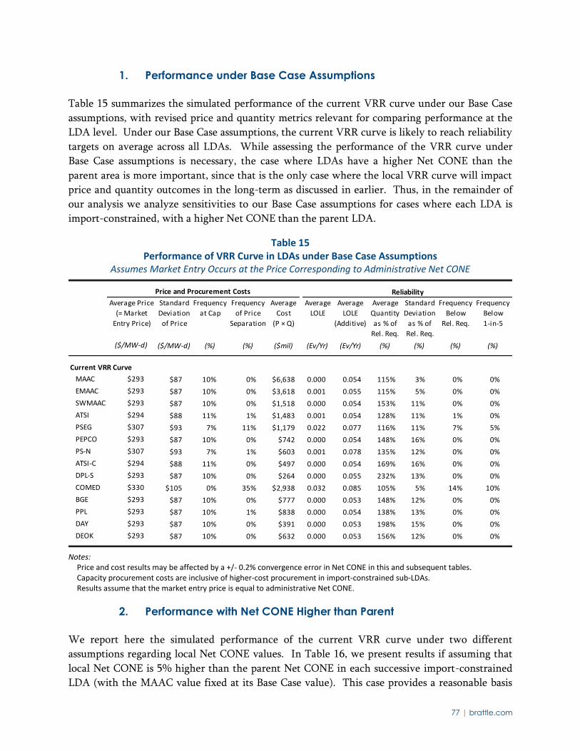
77 | brattle.com

1. Performance under Base Case Assumptions

Table 15 summarizes the simulated performance of the current VRR curve under our Base Case

assumptions, with revised price and quantity metrics relevant for comparing performance at the

LDA level. Under our Base Case assumptions, the current VRR curve is likely to reach reliability

targets on average across all LDAs. While assessing the performance of the VRR curve under

Base Case assumptions is necessary, the case where LDAs have a higher Net CONE than the

parent area is more important, since that is the only case where the local VRR curve will impact

price and quantity outcomes in the long-term as discussed in earlier. Thus, in the remainder of

our analysis we analyze sensitivities to our Base Case assumptions for cases where each LDA is

import-constrained, with a higher Net CONE than the parent LDA.

Table 15 Performance of VRR Curve in LDAs under Base Case Assumptions

Assumes Market Entry Occurs at the Price Corresponding to Administrative Net CONE

Notes:

Price and cost results may be affected by a +/- 0.2% convergence error in Net CONE in this and subsequent tables. Capacity procurement costs are inclusive of higher-cost procurement in import-constrained sub-LDAs.

Results assume that the market entry price is equal to administrative Net CONE.

2. Performance with Net CONE Higher than Parent

We report here the simulated performance of the current VRR curve under two different

assumptions regarding local Net CONE values. In Table 16, we present results if assuming that

local Net CONE is 5% higher than the parent Net CONE in each successive import-constrained

LDA (with the MAAC value fixed at its Base Case value). This case provides a reasonable basis


P

r

Average Price

(= Market

Entry Price)

Standard

Deviation

of Price

Frequency

at Cap

Frequency

of Price

Separation

Average

Cost

(P × Q)

Average

LOLE

Average

LOLE

(Additive)

Average

Quantity

as % of

Rel. Req.

Standard

Deviation

as % of

Rel. Req.

Frequency

Below

Rel. Req.

Frequency

Below

1-in-5

($/MW-d) ($/MW-d) (%) (%) ($mil) (Ev/Yr) (Ev/Yr) (%) (%) (%) (%)

Current VRR Curve

MAAC $293 $87 10% 0% $6,638 0.000 0.054 115% 3% 0% 0%

EMAAC $293 $87 10% 0% $3,618 0.001 0.055 115% 5% 0% 0%

SWMAAC $293 $87 10% 0% $1,518 0.000 0.054 153% 11% 0% 0%

ATSI $294 $88 11% 1% $1,483 0.001 0.054 128% 11% 1% 0%

PSEG $307 $93 7% 11% $1,179 0.022 0.077 116% 11% 7% 5%

PEPCO $293 $87 10% 0% $742 0.000 0.054 148% 16% 0% 0%

PS-N $307 $93 7% 1% $603 0.001 0.078 135% 12% 0% 0%

ATSI-C $294 $88 11% 0% $497 0.000 0.054 169% 16% 0% 0%

DPL-S $293 $87 10% 0% $264 0.000 0.055 232% 13% 0% 0%

COMED $330 $105 0% 35% $2,938 0.032 0.085 105% 5% 14% 10%

BGE $293 $87 10% 0% $777 0.000 0.053 148% 12% 0% 0%

PPL $293 $87 10% 1% $838 0.000 0.054 138% 13% 0% 0%

DAY $293 $87 10% 0% $391 0.000 0.053 198% 15% 0% 0%

DEOK $293 $87 10% 0% $632 0.000 0.053 156% 12% 0% 0%

78 | brattle.com

for evaluating the performance of the VRR Curve under typical conditions, where more import-

constrained locations do show higher net investment costs but are only modestly higher than

elsewhere.

In Table 16, we show a more stressed case in which Net CONE is 5% higher in each LDA (as in

the first case) but the lowest-level LDAs (PS-North, DPL-South, PepCo, BGE, PPL, ATSI-C,

ComEd, Dayton, and DEOK) have a substantially higher Net CONE that is 20% above the parent

LDA value. For example, PS-North would have a 39% higher Net CONE than the Rest of RTO.

This provides an illustration of the VRR curve performance in locations with much higher

investment costs associated with siting difficulties, environmental restrictions, or lack of

available gas and electric infrastructure. In both cases, we assume that the administrative Net

CONE is accurate and equal to the actual price at which developers will enter the market.

Under the 5% higher case, we observe that the current VRR curve falls short of the local

resource adequacy requirement of 1-in-25 (or 0.04 LOLE) in five of the fourteen LDAs. For ease

of reference, we highlight the locations that fall short of these thresholds in all tables reported in

this and the following sections.

In the more stressed case reflected in Table 17, we see that all of the locations with Net CONE

20% above the parent all fail to meet the reliability objective. The poorest-performing LDAs in

this case are some of the most import-dependent locations, such as PepCo and Dayton.

These results demonstrate that the current VRR curve will achieve local reliability objectives in

some of the LDAs but fail to do so in highly import-dependent LDAs. We discuss our

recommendations for locational curves to prevent the susceptibility of low reliability in Section

V.D.

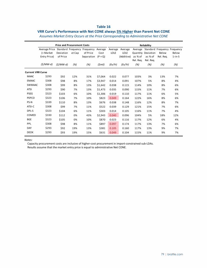
79 | brattle.com

Table 16 VRR Curve’s Performance with Net CONE always 5% Higher than Parent Net CONE

Assumes Market Entry Occurs at the Price Corresponding to Administrative Net CONE

Notes: Capacity procurement costs are inclusive of higher-cost procurement in import-constrained sub-LDAs.

Results assume that the market entry price is equal to administrative Net CONE.


P

r

Average Price

(= Market

Entry Price)

Standard

Deviation

of Price

Frequency

at Cap

Frequency

of Price

Separation

Average

Cost

(P × Q)

Average

LOLE

Average

LOLE

(Additive)

Average

Quantity

as % of

Rel. Req.

Standard

Deviation

as % of

Rel. Req.

Frequency

Below

Rel. Req.

Frequency

Below

1-in-5


Current VRR Curve

MAAC $293 $92 12% 31% $7,064 0.022 0.077 103% 3% 13% 7%

EMAAC $308 $98 8% 17% $3,947 0.014 0.091 107% 5% 8% 4%

SWMAAC $308 $99 8% 13% $1,642 0.038 0.115 114% 10% 8% 6%

ATSI $293 $90 7% 13% $1,473 0.035 0.090 115% 11% 7% 6%

PSEG $323 $103 6% 10% $1,306 0.019 0.110 117% 11% 6% 5%

PEPCO $323 $106 7% 10% $823 0.049 0.164 122% 16% 8% 6%

PS-N $339 $110 8% 13% $676 0.038 0.148 116% 12% 8% 7%

ATSI-C $308 $99 7% 11% $522 0.039 0.129 121% 15% 7% 6%

DPL-S $323 $104 6% 11% $303 0.014 0.105 116% 11% 7% 4%

COMED $330 $112 0% 43% $2,943 0.040 0.096 104% 5% 18% 12%

BGE $323 $105 0% 10% $870 0.023 0.116 117% 12% 6% 4%

PPL $308 $98 8% 11% $897 0.097 0.174 117% 13% 7% 6%

DAY $293 $92 19% 13% $381 0.105 0.160 117% 13% 9% 7%

DEOK $293 $93 19% 15% $631 0.049 0.104 115% 11% 9% 7%

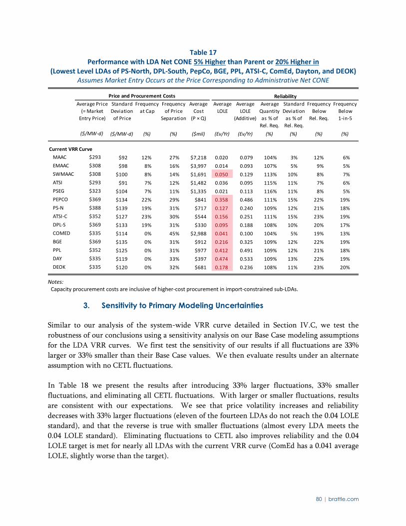
80 | brattle.com

Table 17 Performance with LDA Net CONE 5% Higher than Parent or 20% Higher in

(Lowest Level LDAs of PS-North, DPL-South, PepCo, BGE, PPL, ATSI-C, ComEd, Dayton, and DEOK) Assumes Market Entry Occurs at the Price Corresponding to Administrative Net CONE


3. Sensitivity to Primary Modeling Uncertainties

Similar to our analysis of the system-wide VRR curve detailed in Section IV.C, we test the

robustness of our conclusions using a sensitivity analysis on our Base Case modeling assumptions

for the LDA VRR curves. We first test the sensitivity of our results if all fluctuations are 33%

larger or 33% smaller than their Base Case values. We then evaluate results under an alternate

assumption with no CETL fluctuations.

In Table 18 we present the results after introducing 33% larger fluctuations, 33% smaller

fluctuations, and eliminating all CETL fluctuations. With larger or smaller fluctuations, results

are consistent with our expectations. We see that price volatility increases and reliability

decreases with 33% larger fluctuations (eleven of the fourteen LDAs do not reach the 0.04 LOLE

standard), and that the reverse is true with smaller fluctuations (almost every LDA meets the

0.04 LOLE standard). Eliminating fluctuations to CETL also improves reliability and the 0.04

LOLE target is met for nearly all LDAs with the current VRR curve (ComEd has a 0.041 average

LOLE, slightly worse than the target).


P

r

Average Price

(= Market

Entry Price)

Standard

Deviation

of Price

Frequency

at Cap

Frequency

of Price

Separation

Average

Cost

(P × Q)

Average

LOLE

Average

LOLE

(Additive)

Average

Quantity

as % of

Rel. Req.

Standard

Deviation

as % of

Rel. Req.

Frequency

Below

Rel. Req.

Frequency

Below

1-in-5


Current VRR Curve

MAAC $293 $92 12% 27% $7,218 0.020 0.079 104% 3% 12% 6%

EMAAC $308 $98 8% 16% $3,997 0.014 0.093 107% 5% 9% 5%

SWMAAC $308 $100 8% 14% $1,691 0.050 0.129 113% 10% 8% 7%

ATSI $293 $91 7% 12% $1,482 0.036 0.095 115% 11% 7% 6%

PSEG $323 $104 7% 11% $1,335 0.021 0.113 116% 11% 8% 5%

PEPCO $369 $134 22% 29% $841 0.358 0.486 111% 15% 22% 19%

PS-N $388 $139 19% 31% $717 0.127 0.240 109% 12% 21% 18%

ATSI-C $352 $127 23% 30% $544 0.156 0.251 111% 15% 23% 19%

DPL-S $369 $133 19% 31% $330 0.095 0.188 108% 10% 20% 17%

COMED $335 $114 0% 45% $2,988 0.041 0.100 104% 5% 19% 13%

BGE $369 $135 0% 31% $912 0.216 0.325 109% 12% 22% 19%

PPL $352 $125 0% 31% $977 0.412 0.491 109% 12% 21% 18%

DAY $335 $119 0% 33% $397 0.474 0.533 109% 13% 22% 19%

DEOK $335 $120 0% 32% $681 0.178 0.236 108% 11% 23% 20%

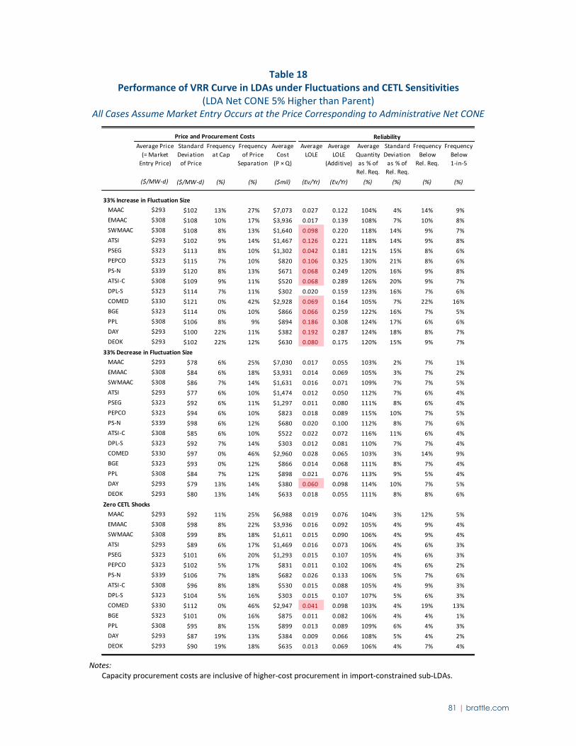
81 | brattle.com

Table 18 Performance of VRR Curve in LDAs under Fluctuations and CETL Sensitivities

(LDA Net CONE 5% Higher than Parent) All Cases Assume Market Entry Occurs at the Price Corresponding to Administrative Net CONE

Notes:

Capacity procurement costs are inclusive of higher-cost procurement in import-constrained sub-LDAs.


P

r

Average Price

(= Market

Entry Price)

Standard

Deviation

of Price

Frequency

at Cap

Frequency

of Price

Separation

Average

Cost

(P × Q)

Average

LOLE

Average

LOLE

(Additive)

Average

Quantity

as % of

Rel. Req.

Standard

Deviation

as % of

Rel. Req.

Frequency

Below

Rel. Req.

Frequency

Below

1-in-5


33% Increase in Fluctuation Size

MAAC $293 $102 13% 27% $7,073 0.027 0.122 104% 4% 14% 9%

EMAAC $308 $108 10% 17% $3,936 0.017 0.139 108% 7% 10% 8%

SWMAAC $308 $108 8% 13% $1,640 0.098 0.220 118% 14% 9% 7%

ATSI $293 $102 9% 14% $1,467 0.126 0.221 118% 14% 9% 8%

PSEG $323 $113 8% 10% $1,302 0.042 0.181 121% 15% 8% 6%

PEPCO $323 $115 7% 10% $820 0.106 0.325 130% 21% 8% 6%

PS-N $339 $120 8% 13% $671 0.068 0.249 120% 16% 9% 8%

ATSI-C $308 $109 9% 11% $520 0.068 0.289 126% 20% 9% 7%

DPL-S $323 $114 7% 11% $302 0.020 0.159 123% 16% 7% 6%

COMED $330 $121 0% 42% $2,928 0.069 0.164 105% 7% 22% 16%

BGE $323 $114 0% 10% $866 0.066 0.259 122% 16% 7% 5%

PPL $308 $106 8% 9% $894 0.186 0.308 124% 17% 6% 6%

DAY $293 $100 22% 11% $382 0.192 0.287 124% 18% 8% 7%

DEOK $293 $102 22% 12% $630 0.080 0.175 120% 15% 9% 7%

33% Decrease in Fluctuation Size

MAAC $293 $78 6% 25% $7,030 0.017 0.055 103% 2% 7% 1%

EMAAC $308 $84 6% 18% $3,931 0.014 0.069 105% 3% 7% 2%

SWMAAC $308 $86 7% 14% $1,631 0.016 0.071 109% 7% 7% 5%

ATSI $293 $77 6% 10% $1,474 0.012 0.050 112% 7% 6% 4%

PSEG $323 $92 6% 11% $1,297 0.011 0.080 111% 8% 6% 4%

PEPCO $323 $94 6% 10% $823 0.018 0.089 115% 10% 7% 5%

PS-N $339 $98 6% 12% $680 0.020 0.100 112% 8% 7% 6%

ATSI-C $308 $85 6% 10% $522 0.022 0.072 116% 11% 6% 4%

DPL-S $323 $92 7% 14% $303 0.012 0.081 110% 7% 7% 4%

COMED $330 $97 0% 46% $2,960 0.028 0.065 103% 3% 14% 9%

BGE $323 $93 0% 12% $866 0.014 0.068 111% 8% 7% 4%

PPL $308 $84 7% 12% $898 0.021 0.076 113% 9% 5% 4%

DAY $293 $79 13% 14% $380 0.060 0.098 114% 10% 7% 5%

DEOK $293 $80 13% 14% $633 0.018 0.055 111% 8% 8% 6%

Zero CETL Shocks

MAAC $293 $92 11% 25% $6,988 0.019 0.076 104% 3% 12% 5%

EMAAC $308 $98 8% 22% $3,936 0.016 0.092 105% 4% 9% 4%

SWMAAC $308 $99 8% 18% $1,611 0.015 0.090 106% 4% 9% 4%

ATSI $293 $89 6% 17% $1,469 0.016 0.073 106% 4% 6% 3%

PSEG $323 $101 6% 20% $1,293 0.015 0.107 105% 4% 6% 3%

PEPCO $323 $102 5% 17% $831 0.011 0.102 106% 4% 6% 2%

PS-N $339 $106 7% 18% $682 0.026 0.133 106% 5% 7% 6%

ATSI-C $308 $96 8% 18% $530 0.015 0.088 105% 4% 9% 3%

DPL-S $323 $104 5% 16% $303 0.015 0.107 107% 5% 6% 3%

COMED $330 $112 0% 46% $2,947 0.041 0.098 103% 4% 19% 13%

BGE $323 $101 0% 16% $875 0.011 0.082 106% 4% 4% 1%

PPL $308 $95 8% 15% $899 0.013 0.089 109% 6% 4% 3%

DAY $293 $87 19% 13% $384 0.009 0.066 108% 5% 4% 2%

DEOK $293 $90 19% 18% $635 0.013 0.069 106% 4% 7% 4%

82 | brattle.com

4. Sensitivity to Administrative Errors in Net CONE

The reliability risks introduced by the potential for errors in Net CONE are even more important

at the LDA level than on a system-wide basis, although we view these as important risks in both

cases. We view these risks as more important at the LDA level partly because we believe the

potential for errors in Net CONE is greater at the LDA level, particularly for the smallest LDAs

for which there is no location-specific Gross CONE or E&AS estimate. Adopting more location-

specific Net CONE estimates will reduce these risks, but small LDAs will still be at greater risk

for Net CONE estimation error. This is because the smallest LDAs are the most prone to

idiosyncratic siting, environmental, or infrastructure limitations that do not apply in the larger

CONE Area. Further, these locations are unlikely to have a substantial number of units similar

to the reference unit, and so calibrating E&AS to plant actual data will not be possible.

Similar to the system level, over-estimating Net CONE results in improved reliability and

increased price volatility while under-estimating Net CONE results in significantly worse

reliability and lower price volatility because of a lower price cap. Table 19 reports the results for

each LDA under these sensitivities and shows nearly all LDAs do not achieve the 0.04

conditional LOLE standard when Net CONE is under-estimated (EMAAC is the only LDA that

meets the 0.04 LOLE target). This suggests again that the administrative Net CONE estimation

has significant implications for the reliability of the VRR curve due to its impact on the price cap.

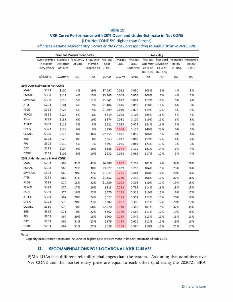
83 | brattle.com

Table 19 VRR Curve Performance with 20% Over- and Under-Estimate in Net CONE

(LDA Net CONE 5% Higher than Parent) All Cases Assume Market Entry Occurs at the Price Corresponding to Administrative Net CONE


D. RECOMMENDATIONS FOR LOCATIONAL VRR CURVES

PJM’s LDAs face different reliability challenges than the system. Assuming that administrative

Net CONE and the market entry price are equal to each other (and using the 2020/21 BRA


P

r

Average Price

(= Market

Entry Price)

Standard

Deviation

of Price

Frequency

at Cap

Frequency

of Price

Separation

Average

Cost

(P × Q)

Average

LOLE

Average

LOLE

(Additive)

Average

Quantity

as % of

Rel. Req.

Standard

Deviation

as % of

Rel. Req.

Frequency

Below

Rel. Req.

Frequency

Below

1-in-5


20% Over-Estimate in Net CONE

MAAC $293 $100 4% 19% $7,097 0.012 0.050 105% 3% 4% 3%

EMAAC $308 $112 4% 15% $3,945 0.009 0.059 108% 5% 4% 2%

SWMAAC $308 $113 5% 11% $1,641 0.027 0.077 117% 11% 5% 4%

ATSI $293 $101 4% 9% $1,484 0.016 0.053 118% 11% 4% 3%

PSEG $323 $124 5% 9% $1,299 0.019 0.078 119% 12% 5% 4%

PEPCO $323 $127 5% 8% $819 0.028 0.105 125% 16% 5% 4%

PS-N $339 $138 6% 10% $674 0.031 0.109 119% 13% 6% 5%

ATSI-C $308 $115 5% 8% $521 0.025 0.079 124% 16% 5% 4%

DPL-S $323 $128 6% 9% $299 0.064 0.123 140% 22% 6% 5%

COMED $330 $128 0% 36% $2,955 0.021 0.059 106% 5% 9% 6%

BGE $323 $125 0% 8% $863 0.017 0.082 119% 12% 4% 4%

PPL $308 $110 5% 7% $897 0.035 0.084 123% 13% 3% 3%

DAY $293 $104 9% 10% $385 0.074 0.112 121% 14% 6% 4%

DEOK $293 $106 9% 10% $632 0.028 0.066 117% 12% 5% 4%

20% Under-Estimate in Net CONE

MAAC $293 $68 31% 43% $6,989 0.057 0.258 101% 4% 34% 20%

EMAAC $308 $69 22% 30% $3,927 0.039 0.298 104% 5% 23% 16%

SWMAAC $308 $68 20% 23% $1,621 0.225 0.484 108% 10% 20% 16%

ATSI $293 $66 21% 24% $1,452 0.230 0.432 108% 11% 22% 18%

PSEG $323 $70 18% 22% $1,289 0.098 0.395 110% 11% 19% 15%

PEPCO $323 $70 17% 20% $813 0.252 0.735 114% 16% 18% 15%

PS-N $339 $70 18% 23% $670 0.123 0.518 110% 12% 19% 17%

ATSI-C $308 $67 20% 24% $522 0.123 0.554 112% 15% 20% 16%

DPL-S $323 $70 20% 23% $302 0.097 0.395 111% 12% 20% 17%

COMED $330 $75 0% 60% $2,920 0.140 0.342 101% 5% 42% 35%

BGE $323 $71 0% 22% $862 0.140 0.567 111% 12% 19% 15%

PPL $308 $67 20% 18% $900 0.284 0.542 113% 13% 15% 13%

DAY $293 $65 51% 23% $376 0.424 0.626 112% 13% 19% 16%

DEOK $293 $67 51% 23% $628 0.158 0.360 110% 11% 21% 17%

84 | brattle.com

parameters, similar to Section IV.C), local VRR curves perform well.82 However, under potential

future conditions where market entry prices in the LDAs exceed those in the parent, we

identified several concerns. Under these conditions, the smaller size of LDAs relative to

fluctuations in local net supply make it more difficult to attract investment and lead to reliability

challenges.

Our simulations demonstrate these risks and show that the existing VRR curves would often not

achieve the 1-in-25 conditional target if LDA Net CONE were greater than parent Net CONE,

with the greatest susceptibility in the most import-dependent LDAs and LDAs with Net CONE

substantially above the parent LDA Net CONE. To ensure more robust performance from a

reliability perspective, provide more price stability, and produce prices that are more reflective of

local reliability value, we recommend that PJM and stakeholders consider the following changes

to local VRR curves:

1. Impose a minimum curve width equal to 25% of CETL. We find that the current VRR

curve would not achieve the local reliability objective in a realistic stress scenario with

LDA Net CONE substantially above the parent level. Performance is worst in the

smallest, most import-dependent zones. To address this gap, we find that applying a

minimum curve width based on CETL to be a targeted and effective way to improve

performance.83 See Table 20. This minimum curve width could be applied to local curves

of the same shape as any of the candidate system curves from Figure ES-1.

2. Ensure the LDA price cap is at least 1.7 × Net CONE. We find that a price cap of at least

1.7 × Net CONE substantially improves simulated reliability outcomes in LDAs because it

introduces stronger price signals when supplies become scarce. The prospect of higher

prices during low reliability outcomes provides greater incentives for suppliers to locate

there rather than in the parent LDA. If PJM adopts our recommended system curve

based on CC Net CONE, with a 1% left-shift and 70% Gross CONE price cap (curve E in

Figure ES-1), the price cap will already be approximately 1.8 × Net CONE. No further

change is needed if this curve is applied at the local level. See Table 20.

82 If PJM adopted a VRR curve anchored on a Net CONE value considerably greater than the market

entry price, such as curve A or curve B in Figure ES-1, the LDAs would become even more reliable.

83 We have not performed a detailed assessment of the locational performance of a 1% left-shifted curve.

It is possible that the left shift would slightly reduce reliability in the LDAs and require a slightly

wider curve to accommodate.

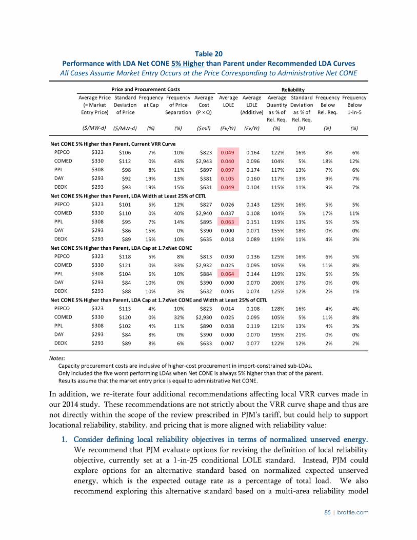
85 | brattle.com

Table 20 Performance with LDA Net CONE 5% Higher than Parent under Recommended LDA Curves

All Cases Assume Market Entry Occurs at the Price Corresponding to Administrative Net CONE

Notes:

Capacity procurement costs are inclusive of higher-cost procurement in import-constrained sub-LDAs. Only included the five worst performing LDAs when Net CONE is always 5% higher than that of the parent. Results assume that the market entry price is equal to administrative Net CONE.

In addition, we re-iterate four additional recommendations affecting local VRR curves made in

our 2014 study. These recommendations are not strictly about the VRR curve shape and thus are

not directly within the scope of the review prescribed in PJM’s tariff, but could help to support

locational reliability, stability, and pricing that is more aligned with reliability value:

1. Consider defining local reliability objectives in terms of normalized unserved energy.

We recommend that PJM evaluate options for revising the definition of local reliability

objective, currently set at a 1-in-25 conditional LOLE standard. Instead, PJM could

explore options for an alternative standard based on normalized expected unserved

energy, which is the expected outage rate as a percentage of total load. We also

recommend exploring this alternative standard based on a multi-area reliability model


P

r

Average Price

(= Market

Entry Price)

Standard

Deviation

of Price

Frequency

at Cap

Frequency

of Price

Separation

Average

Cost

(P × Q)

Average

LOLE

Average

LOLE

(Additive)

Average

Quantity

as % of

Rel. Req.

Standard

Deviation

as % of

Rel. Req.

Frequency

Below

Rel. Req.

Frequency

Below

1-in-5


Net CONE 5% Higher than Parent, Current VRR Curve

PEPCO $323 $106 7% 10% $823 0.049 0.164 122% 16% 8% 6%

COMED $330 $112 0% 43% $2,943 0.040 0.096 104% 5% 18% 12%

PPL $308 $98 8% 11% $897 0.097 0.174 117% 13% 7% 6%

DAY $293 $92 19% 13% $381 0.105 0.160 117% 13% 9% 7%

DEOK $293 $93 19% 15% $631 0.049 0.104 115% 11% 9% 7%

Net CONE 5% Higher than Parent, LDA Width at Least 25% of CETL

PEPCO $323 $101 5% 12% $827 0.026 0.143 125% 16% 5% 5%

COMED $330 $110 0% 40% $2,940 0.037 0.108 104% 5% 17% 11%

PPL $308 $95 7% 14% $895 0.063 0.151 119% 13% 5% 5%

DAY $293 $86 15% 0% $390 0.000 0.071 155% 18% 0% 0%

DEOK $293 $89 15% 10% $635 0.018 0.089 119% 11% 4% 3%

Net CONE 5% Higher than Parent, LDA Cap at 1.7xNet CONE

PEPCO $323 $118 5% 8% $813 0.030 0.136 125% 16% 6% 5%

COMED $330 $121 0% 33% $2,932 0.025 0.095 105% 5% 11% 8%

PPL $308 $104 6% 10% $884 0.064 0.144 119% 13% 5% 5%

DAY $293 $84 10% 0% $390 0.000 0.070 206% 17% 0% 0%

DEOK $293 $88 10% 3% $632 0.005 0.074 125% 12% 2% 1%

Net CONE 5% Higher than Parent, LDA Cap at 1.7xNet CONE and Width at Least 25% of CETL

PEPCO $323 $113 4% 10% $823 0.014 0.108 128% 16% 4% 4%

COMED $330 $120 0% 32% $2,930 0.025 0.095 105% 5% 11% 8%

PPL $308 $102 4% 11% $890 0.038 0.119 121% 13% 4% 3%

DAY $293 $84 8% 0% $390 0.000 0.070 195% 21% 0% 0%

DEOK $293 $89 8% 6% $633 0.007 0.077 122% 12% 2% 2%

86 | brattle.com

that simultaneously estimates the location-specific EUE among different PJM system and

sub-regions. The result would be a reliability standard that better accounts for the level

of correlation between system-wide and local generation outages, and results in a more

uniform level of reliability for LDAs of different sizes and import dependence.

2. Consider alternatives to the “nested” LDA structure. We recommend that PJM consider

generalizing its approach to modeling locational constraints in RPM beyond import-

constrained, nested LDAs with a single import limit. As the number of modeled LDAs

increases and the system reserve margin decreases, different types of constraints may

emerge that do not correspond to a strictly nested model. A more generalized “meshed”

LDA model (with simultaneous clearing during the auction) would explicitly allow for

the possibility that some locations may be export-constrained, that some LDAs may have

multiple transmission import paths, and some may have the possibility of being either

import- or export-constrained, depending on RPM auction outcomes.84

3. Evaluate options for increasing stability of CETL. We recommend that PJM continue to

review its options for increasing the predictability and stability of its CETL estimates.

Based on our simulation results, we find that reducing CETL uncertainty could

significantly reduce capacity price volatility in LDAs. Physical changes to the

transmission system do need to continue to be reflected as changes in CETL, but reducing

uncertainty would provide substantial benefits in reducing price volatility. We suggested

several options to evaluate for mitigating volatility in CETL in our 2011 RPM Review.

4. Consider revising the RPM auction clearing mechanics within LDAs based on delivered

reliability value. As another option for enhancing locational capacity price stability and

overall efficiency, we recommend that PJM consider revising its auction-clearing

mechanics to produce prices that are more proportional to the marginal reliability value

of incremental resources in each LDA. Such a mechanism would determine the lowest-

cost resources for achieving local reliability objectives by selecting either: (a) a greater

quantity of lower-cost imports from outside the LDA, but recognizing the lower

reliability of imported resources (due to transmission import capability risk and lost

diversity benefits as an LDA becomes more import-dependent); or (b) a smaller quantity

of locally-sourced resources with greater reliability value (i.e., without the additional

transmission availability risk). This approach would stabilize LDA pricing by allowing

for more gradual price separation as an LDA becomes more import-dependent (rather

than price-separating only once the administratively-set import constraints bind).85

84 The IMM recently recommended that PJM implement a nodal capacity market. The principle

underlying the IMM’s recommendation—to align more closely the market with the characteristics of

the actual electrical facts of the grid—is the same principle that motivates our recommendation to

consider alternatives to the “nested” LDA structure. See Monitoring Analytics (2017).

85 See our 2014 study for a more detailed discussion on clearing mechanics for locational reliability

value, Pfeifenberger (2014). ISO-NE recently implemented their Marginal Reliability Impact based

demand curves to address this in their market, see ISO-NE (2016).

87 | brattle.com

List of Acronyms

A/S Ancillary Service

AESO Alberta Electricity System Operator

ATSI American Transmission Systems, Inc. (a FirstEnergy subsidiary)

ATSI-C American Transmission Systems, Inc.-Cleveland

ATWACC After-Tax Weighted-Average Cost Of Capital

BGE Baltimore Gas and Electric Company

BLS Bureau of Labor Statistics

BRA Base Residual Auction

CC Combined Cycle

CETL Capacity Emergency Transfer Limit

ComEd Commonwealth Edison, Exelon Corporation

CONE Cost of New Entry

CT Combustion Turbine

CP Capacity Performance

Dayton Dayton Power and Light Company, aka DAY

DEOK Duke Energy Ohio/Kentucky

DPL-South Delmarva Power and Light-South

DR Demand Response

E&AS Energy and Ancillary Services

EKPC East Kentucky Power Cooperative, Inc.

EMAAC Eastern Mid-Atlantic Area Council

EUE Expected Unserved Energy

FERC Federal Energy Regulatory Commission

FOM Fixed Operation and Maintenance

FPR Forecast Pool Requirement

FRR Fixed Resource Requirement

IA Incremental Auction

IMM Independent Market Monitor

IRM Installed Reserve Margin

ISO Independent System Operator

ISO-NE ISO New England

kW Kilowatt

kWh Kilowatt Hours

88 | brattle.com

LDA Locational Deliverability Area

LMP Locational Marginal Price

LOLE Loss of Load Event

LSE Load-Serving Entities

MAAC Mid-Atlantic Area Council

MetEd Metropolitan Edison Company

MISO Midcontinent Independent System Operator

MOPR Minimum Offer Price Rule

MW Megawatts

MWh Megawatt Hours

NYISO New York ISO

OATT Open Access Transmission Tariff

PECO PECO Energy Company, Exelon Corporation, aka PE

PenElec Pennsylvania Electric Company

PepCo Potomac Electric Power Company

PJM PJM Interconnection, LLC

PPL Pennsylvania Power and Light Company

PS-North Public Service Enterprise Group-North

PSEG Public Service Enterprise Group

PSEG North Public Service Enterprise Group-North

RPM Reliability Pricing Model

RTO Regional Transmission Organization

SCR Selective Catalytic Reduction

SWMAAC Southwestern Mid-Atlantic Area Council

UCAP Unforced Capacity

VOM Variable Operations and Maintenance

VRR Variable Resource Requirement

WMAAC Western Mid-Atlantic Area Council

89 | brattle.com

Bibliography

Federal Energy Regulatory Commission (2014). Order Conditionally Accepting Tariff Revisions

Subject to Compliance Filing, Issued November 28, 2014. Docket No. ER14-2940-000.

Federal Energy Regulatory Commission (2017). Order Accepting Filing, Issued October 6, 2017.

Docket No. ER17-795-000.

ISO New England (2016). FCA 11 MRI Base System-wide and Zonal Sloped Demand Curves, October 4, 2016. Retrieved from: https://www.iso-ne.com/static-

assets/documents/2016/09/a2_fca11_demand_curves.pdf

ISO New England, Inc., (2017). “RE: ISO New England Inc.; Filing of CONE and ORTP Updates,”

January 13, 2017. Docket No. ER17-795-000. Retrieved from: https://iso-ne.com/static-

assets/documents/2017/01/cone_and_ortp_updates.pdf

Monitoring Analytics (2014). State of the Market Reports. Available at:

http://www.monitoringanalytics.com/reports/PJM_State_of_the_Market/2014.shtml

Monitoring Analytics (2017). State of the Market Reports. Available at:


Newell, Samuel., J. Michael Hagerty, Johannes P. Pfeifenberger, Bin Zhou, Emily Shorin, Perry

Fitz (2018). PJM Cost of New Entry: Combustion Turbines and Combined-Cycle Plants with June 1, 2022 Online Date, February 2018.

New York Independent System Operator (2017). Manual 4: Installed Capacity Manual, August

2017. Retrieved from:

http://www.nyiso.com/public/webdocs/markets_operations/documents/Manuals_and_Guides

/Manuals/Operations/icap_mnl.pdf

Potomac Economics (2017). “Concept for Locational Capacity Pricing Based on Marginal

Reliability Impacts and Costs,” June 22, 2017. Retrieved from:

http://www.nyiso.com/public/webdocs/markets_operations/committees/bic_icapwg/meeting_

materials/2017-06-22/SOM%20Recommendation%202013-

1c%20re%20Capacity%20Pricing_ICAPWG_6-22-2017.pdf

Pfeifenberger, Johannes P., Samuel A. Newell, Robert Earle, Attila Hajos, and Mariko Geronimo

(2008). Review of PJM’s Reliability Pricing Model (RPM), June 30, 2008. Retrieved from:

http://brattle.com/system/publications/pdfs/000/004/728/original/Review_of_PJM's_Reliabilit

y_Pricing_Model_Pfeifenberger_et_al_Jun_30_2008.pdf?1378772125

Pfeifenberger, Johannes P., Samuel A. Newell, Kathleen Spees, Attila Hajos, and Kamen

Madjarov (2011). Second Performance Assessment of PJM's Reliability Pricing Model: Market

https://www.iso-ne.com/static-assets/documents/2016/09/a2_fca11_demand_curves.pdf

https://www.iso-ne.com/static-assets/documents/2016/09/a2_fca11_demand_curves.pdf



http://www.nyiso.com/public/webdocs/markets_operations/documents/Manuals_and_Guides/Manuals/Operations/icap_mnl.pdf

http://www.nyiso.com/public/webdocs/markets_operations/documents/Manuals_and_Guides/Manuals/Operations/icap_mnl.pdf

http://www.nyiso.com/public/webdocs/markets_operations/committees/bic_icapwg/meeting_materials/2017-06-22/SOM%20Recommendation%202013-1c%20re%20Capacity%20Pricing_ICAPWG_6-22-2017.pdf



http://brattle.com/system/publications/pdfs/000/004/728/original/Review_of_PJM's_Reliability_Pricing_Model_Pfeifenberger_et_al_Jun_30_2008.pdf?1378772125

http://brattle.com/system/publications/pdfs/000/004/728/original/Review_of_PJM's_Reliability_Pricing_Model_Pfeifenberger_et_al_Jun_30_2008.pdf?1378772125

90 | brattle.com

Results 2007/08 through 2014/15, August 26, 2011. Retrieved from:

http://www.brattle.com/system/publications/pdfs/000/004/833/original/Second_Performance

_Assessment_of_PJM's_Reliability_Pricing_Model_Pfeifenberger_et_al_Aug_26_2011.pdf?13

78772133

Pfeifenberger, Johannes P., Kathleen Spees, Kevin Carden, and Nick Wintermantel (2013).

Resource Adequacy Requirements: Reliability and Economic Implications, September 2013.

Retrieved from:

http://www.brattle.com/system/news/pdfs/000/000/618/original/Resource_Adequacy_Requir

ements_-_Reliability_and_Economic_Requirements.pdf?1392126844

Pfeifenberger, Johannes P., Samuel A. Newell, Kathleen Spees, Ann Murray, and Ioanna

Karkatsouli (2014). Third Triennial Review of PJM’s Variable Resource Requirement Curve, May 15, 2014. Retrieved from:

http://www.brattle.com/system/publications/pdfs/000/005/009/original/Third_Triennial_Revi

ew_of_PJM's_Variable_Resource_Requirement_Curve.pdf?1400252215

PJM Interconnection, L.L.C. (2005). “Summer 2005 PJM Reliability Assessment,” June 7, 2005.

Retrieved from:

http://www.puc.state.pa.us/electric/pdf/Reliability/PJM_Summer_Reliability2005.pdf

PJM Interconnection, L.L.C. (2006). “Summer 2006 PJM Reliability Assessment,” May 24, 2006.

Retrieved from:


PJM Interconnection, L.L.C. (2007a). “2007 Load Forecast Report,” January 2007. Retrieved from:

http://www.pjm.com/-/media/planning/res-adeq/load-forecast/2007-load-report.ashx?la=en

PJM Interconnection, L.L.C. (2007b). “Summer 2007 PJM Reliability Assessment,” May 30, 2007.

Retrieved from:


PJM Interconnection, L.L.C. (2007c). “2007/08–2009/10 Planning Period Parameters,” October

29, 2007. Retrieved from: http://www.pjm.com/-/media/markets-ops/rpm/rpm-auction-

info/planning-period-parameters.ashx?la=en


http://www.pjm.com/-/media/documents/reports/2008-load-report.ashx?la=en

PJM Interconnection, L.L.C. (2008b). “Summer 2008 PJM Reliability Assessment,” June 12, 2008.

Retrieved from:



http://www.pjm.com/-/media/documents/reports/2009-pjm-load-report.ashx?la=en

http://www.brattle.com/system/publications/pdfs/000/004/833/original/Second_Performance_Assessment_of_PJM's_Reliability_Pricing_Model_Pfeifenberger_et_al_Aug_26_2011.pdf?1378772133



http://www.brattle.com/system/news/pdfs/000/000/618/original/Resource_Adequacy_Requirements_-_Reliability_and_Economic_Requirements.pdf?1392126844

http://www.brattle.com/system/news/pdfs/000/000/618/original/Resource_Adequacy_Requirements_-_Reliability_and_Economic_Requirements.pdf?1392126844

http://www.brattle.com/system/publications/pdfs/000/005/009/original/Third_Triennial_Review_of_PJM's_Variable_Resource_Requirement_Curve.pdf?1400252215

http://www.brattle.com/system/publications/pdfs/000/005/009/original/Third_Triennial_Review_of_PJM's_Variable_Resource_Requirement_Curve.pdf?1400252215



http://www.pjm.com/-/media/planning/res-adeq/load-forecast/2007-load-report.ashx?la=en


http://www.pjm.com/-/media/markets-ops/rpm/rpm-auction-info/planning-period-parameters.ashx?la=en

http://www.pjm.com/-/media/markets-ops/rpm/rpm-auction-info/planning-period-parameters.ashx?la=en

http://www.pjm.com/-/media/documents/reports/2008-load-report.ashx?la=en


http://www.pjm.com/-/media/documents/reports/2009-pjm-load-report.ashx?la=en

91 | brattle.com

PJM Interconnection, L.L.C. (2009b). “2012/2013 Planning Period Parameters,” May 22, 2009.

Retrieved from: http://www.pjm.com/-/media/markets-ops/rpm/rpm-auction-info/2012-

2013-rpm-planning-parameters.ashx?la=en

PJM Interconnection, L.L.C. (2009c). “Summer 2009 PJM Reliability Assessment,” June 9, 2009.

Retrieved from:

http://www.puc.state.pa.us/electric/pdf/Reliability/Summer_Reliability_2009-PJM.pdf

PJM Interconnection, L.L.C. (2009d). “2011/2012 Planning Period Parameters,” December 2,

2009. Retrieved from: http://www.pjm.com/-/media/markets-ops/rpm/rpm-auction-

info/2011-2012-rpm-bra-planning-parameters.ashx?la=en

PJM Interconnection, L.L.C. (2009e). “2010/2011 Planning Period Parameters,” December 3,


info/2010-2011-rpm-planning-parameters.ashx?la=en

PJM Interconnection, L.L.C. (2009f). “A Review of Generation Compensation and Cost Elements

in the PJM Markets,” 2009. Retrieved from: http://www.pjm.com/~/media/committees-

groups/committees/mrc/20100120/20100120-item-02-review-of-generation-costs-and-

compensation.ashx


http://www.pjm.com/-/media/documents/reports/2010-load-forecast-report.ashx?la=en



2014-planning-period-parameters.ashx?la=en

PJM Interconnection, L.L.C. (2010c). “Summer 2010 PJM Reliability Assessment,” May 20, 2010.

Retrieved from:



http://www.pjm.com/-/media/library/reports-notices/load-forecast/2011-pjm-load-

report.ashx?la=en

PJM Interconnection, L.L.C. (2011b). “2014/2015 Planning Period Parameters,” April 8, 2011.

Retrieved from: http://www.pjm.com/-/media/markets-ops/rpm/rpm-auction-info/rpm-bra-

planning-parameters-2014-2015.ashx?la=en


Retrieved from:

https://www.puc.state.pa.us/electric/pdf/Reliability/Summer_Reliability_2011-PJM.pdf

http://www.pjm.com/-/media/markets-ops/rpm/rpm-auction-info/2012-2013-rpm-planning-parameters.ashx?la=en



http://www.pjm.com/-/media/markets-ops/rpm/rpm-auction-info/2011-2012-rpm-bra-planning-parameters.ashx?la=en

http://www.pjm.com/-/media/markets-ops/rpm/rpm-auction-info/2011-2012-rpm-bra-planning-parameters.ashx?la=en



http://www.pjm.com/~/media/committees-groups/committees/mrc/20100120/20100120-item-02-review-of-generation-costs-and-compensation.ashx



http://www.pjm.com/-/media/documents/reports/2010-load-forecast-report.ashx?la=en

http://www.pjm.com/-/media/markets-ops/rpm/rpm-auction-info/2013-2014-planning-period-parameters.ashx?la=en



http://www.pjm.com/-/media/library/reports-notices/load-forecast/2011-pjm-load-report.ashx?la=en


http://www.pjm.com/-/media/markets-ops/rpm/rpm-auction-info/rpm-bra-planning-parameters-2014-2015.ashx?la=en

http://www.pjm.com/-/media/markets-ops/rpm/rpm-auction-info/rpm-bra-planning-parameters-2014-2015.ashx?la=en


92 | brattle.com


http://www.pjm.com/-/media/library/reports-notices/load-forecast/2012-pjm-load-

report.ashx?la=en



2016-planning-period-parameters.ashx?la=en


Retrieved from:



http://www.pjm.com/-/media/library/reports-notices/load-forecast/2013-load-forecast-

report.ashx?la=en

PJM Interconnection, L.L.C. (2013b). “Summer 2013 PJM Reliability Assessment,” June 6, 2013.

Retrieved from:

http://www.puc.state.pa.us/Electric/pdf/Reliability/Summer_Reliability_2013-PJM.pdf



report.ashx?la=en

PJM Interconnection, L.L.C. (2014b). “Summer 2014 PJM Reliability Assessment,” June 2014.

Retrieved from: http://www.puc.pa.gov/Electric/pdf/Reliability/Summer_Reliability_2014-

PJM.pdf

PJM Interconnection, L.L.C. (2014c). “2016/2017 Planning Parameters,” June 4, 2014. Retrieved

from: http://www.pjm.com/-/media/markets-ops/rpm/rpm-auction-info/2016-2017-planning-

period-parameters.ashx?la=en

PJM Interconnection, L.L.C. (2014e). “2017/2018 Planning Parameters,” June 4, 2014. Retrieved

from: http://www.pjm.com/-/media/markets-ops/rpm/rpm-auction-info/2017-2018-planning-

period-parameters.ashx?la=en

PJM Interconnection, L.L.C. (2014f). “Revisions to the PJM Open Access Transmission Tariff,”

September 25, 2014. Docket No. ER14-2940-000.



report.ashx?la=en


Retrieved from: http://www.puc.pa.gov/Electric/pdf/Reliability/Summer_Reliability_2015-

PJM.pdf






http://www.pjm.com/-/media/library/reports-notices/load-forecast/2013-load-forecast-report.ashx?la=en





http://www.puc.pa.gov/Electric/pdf/Reliability/Summer_Reliability_2014-PJM.pdf










93 | brattle.com

PJM Interconnection, L.L.C. (2015c). “Capacity Performance Transition Incremental Auctions

Rules, Schedule and Planning Parameters,” July 28, 2015. Retrieved from:

http://www.pjm.com/~/media/markets-ops/rpm/rpm-auction-info/2016-2018-cp-transition-

incremental-auctions-rules-schedule-planning-parameters.ashx

PJM Interconnection, L.L.C. (2015d). “2018/2019 Planning Parameters,” August 27, 2015.


2019-bra-planning-parameters.ashx?la=en

PJM Interconnection, L.L.C. (2015e). “Historical Performance Assessment Hours,” November 16,

2015. Retrieved from: http://www.pjm.com/-/media/committees-

groups/committees/elc/postings/historical-performance-assessment-hours.ashx?la=en


http://www.pjm.com/-/media/library/reports-notices/load-forecast/2016-load-

report.ashx?la=en


Retrieved from:


PJM Interconnection, L.L.C. (2016c). “2019/2020 Planning Parameters,” June 10, 2016. Retrieved

from: http://www.pjm.com/-/media/markets-ops/rpm/rpm-auction-info/2019-2020-bra-

planning-parameters.ashx?la=en



report.ashx?la=en

PJM Interconnection, L.L.C. (2017b). “Final CP Market Seller Offer Cap Values”, January 9, 2017.


2021-final-cp-market-seller-offer-cap-values.ashx?la=en

PJM Interconnection, L.L.C. (2017c). “2020/2021 Planning Parameters,” May 23, 2017. Retrieved

from: http://www.pjm.com/-/media/markets-ops/rpm/rpm-auction-info/2020-2021-bra-

planning-period-parameters.ashx?la=en

PJM Interconnection, L.L.C. (2017d). “2020/2021 RPM Base Residual Auction Results,” May 23,


info/2020-2021-base-residual-auction-report.ashx?la=en

PJM Interconnection, L.L.C. (2017e). “Summer 2017 PJM Reliability Assessment,” June 2017.

Retrieved from:


http://www.pjm.com/~/media/markets-ops/rpm/rpm-auction-info/2016-2018-cp-transition-incremental-auctions-rules-schedule-planning-parameters.ashx

http://www.pjm.com/~/media/markets-ops/rpm/rpm-auction-info/2016-2018-cp-transition-incremental-auctions-rules-schedule-planning-parameters.ashx

http://www.pjm.com/-/media/markets-ops/rpm/rpm-auction-info/2018-2019-bra-planning-parameters.ashx?la=en


http://www.pjm.com/-/media/committees-groups/committees/elc/postings/historical-performance-assessment-hours.ashx?la=en

http://www.pjm.com/-/media/committees-groups/committees/elc/postings/historical-performance-assessment-hours.ashx?la=en

http://www.pjm.com/-/media/library/reports-notices/load-forecast/2016-load-report.ashx?la=en

http://www.pjm.com/-/media/library/reports-notices/load-forecast/2016-load-report.ashx?la=en






http://www.pjm.com/-/media/markets-ops/rpm/rpm-auction-info/2020-2021-final-cp-market-seller-offer-cap-values.ashx?la=en

http://www.pjm.com/-/media/markets-ops/rpm/rpm-auction-info/2020-2021-final-cp-market-seller-offer-cap-values.ashx?la=en

http://www.pjm.com/-/media/markets-ops/rpm/rpm-auction-info/2020-2021-bra-planning-period-parameters.ashx?la=en

http://www.pjm.com/-/media/markets-ops/rpm/rpm-auction-info/2020-2021-bra-planning-period-parameters.ashx?la=en

http://www.pjm.com/-/media/markets-ops/rpm/rpm-auction-info/2020-2021-base-residual-auction-report.ashx?la=en

http://www.pjm.com/-/media/markets-ops/rpm/rpm-auction-info/2020-2021-base-residual-auction-report.ashx?la=en


94 | brattle.com

PJM Interconnection, L.L.C. (2017f). “PJM Manual 18: PJM Capacity Market,” July 27, 2017.

Retrieved from: http://www.pjm.com/-/media/documents/manuals/m18.ashx

PJM Interconnection, L.L.C. (2017g). PJM Manual 18: PJM Capacity Market. Revision 38,

Effective July 27, 2017. Retrieved from:

http://www.pjm.com/~/media/documents/manuals/m18.ashx

PJM Interconnection, L.L.C. (2017h) PJM Open Access Transmission Tariff. Effective October 1,

2017. Retrieved from: http://www.pjm.com/directory/merged-tariffs/oatt.pdf

PJM Interconnection, L.L.C. (2017i). “2017 PJM Reserve Requirement Study,” October 12, 2017.

Retrieved from: http://wired.pjm.com/-/media/committees-

groups/committees/mc/20171026/20171026-item-03-2017-irm-study.ashx

PJM Interconnection, L.L.C. (2018). “2021/2022 Planning Parameters,” February 01, 2018.


2022/2021-2022-bra-planning-period-parameters.ashx?la=en

Weitzman, Martin L. (1974), “Prices vs. Quantities”, The Review of Economic Studies 41(4),

October 1974, pp. 477–491.

http://www.pjm.com/-/media/documents/manuals/m18.ashx

http://www.pjm.com/~/media/documents/manuals/m18.ashx

http://www.pjm.com/directory/merged-tariffs/oatt.pdf

http://wired.pjm.com/-/media/committees-groups/committees/mc/20171026/20171026-item-03-2017-irm-study.ashx

http://wired.pjm.com/-/media/committees-groups/committees/mc/20171026/20171026-item-03-2017-irm-study.ashx

http://www.pjm.com/-/media/markets-ops/rpm/rpm-auction-info/2021-2022/2021-2022-bra-planning-period-parameters.ashx?la=en

http://www.pjm.com/-/media/markets-ops/rpm/rpm-auction-info/2021-2022/2021-2022-bra-planning-period-parameters.ashx?la=en

95 | brattle.com

Appendix A: Magnitude of Monte Carlo Fluctuations

In this appendix we provide additional detail on our approach to estimating and implementing a

realistic magnitude of fluctuations into our Monte Carlo simulation modeling, including

fluctuations to: (1) supply offer quantity; (2) reliability requirement; (3) administrative net

CONE; and (4) CETL. A summary of these fluctuations and the combined supply minus demand

fluctuations in each location is included in Section III.E above.

A. SUPPLY OFFER QUANTITY

We estimate gross supply fluctuations based on the range of actual total supply offer quantities in

historical BRAs over delivery years 2009/10 to 2020/21, based on offer data provided by PJM.

Table 21 summarizes the total supply offered by LDA, as well as several series of historical

fluctuations calculated in different ways, based on the distributions of total supply offers, year-

to-year changes in supply offers, and differences in supply offers relative to a linear time trend

and spline interpolation time trend. We determine reasonable supply fluctuations magnitudes

based on the historical fluctuations as an exponential function of LDA size, resulting in the final

supply fluctuations values shown in column 9 of Table 21.

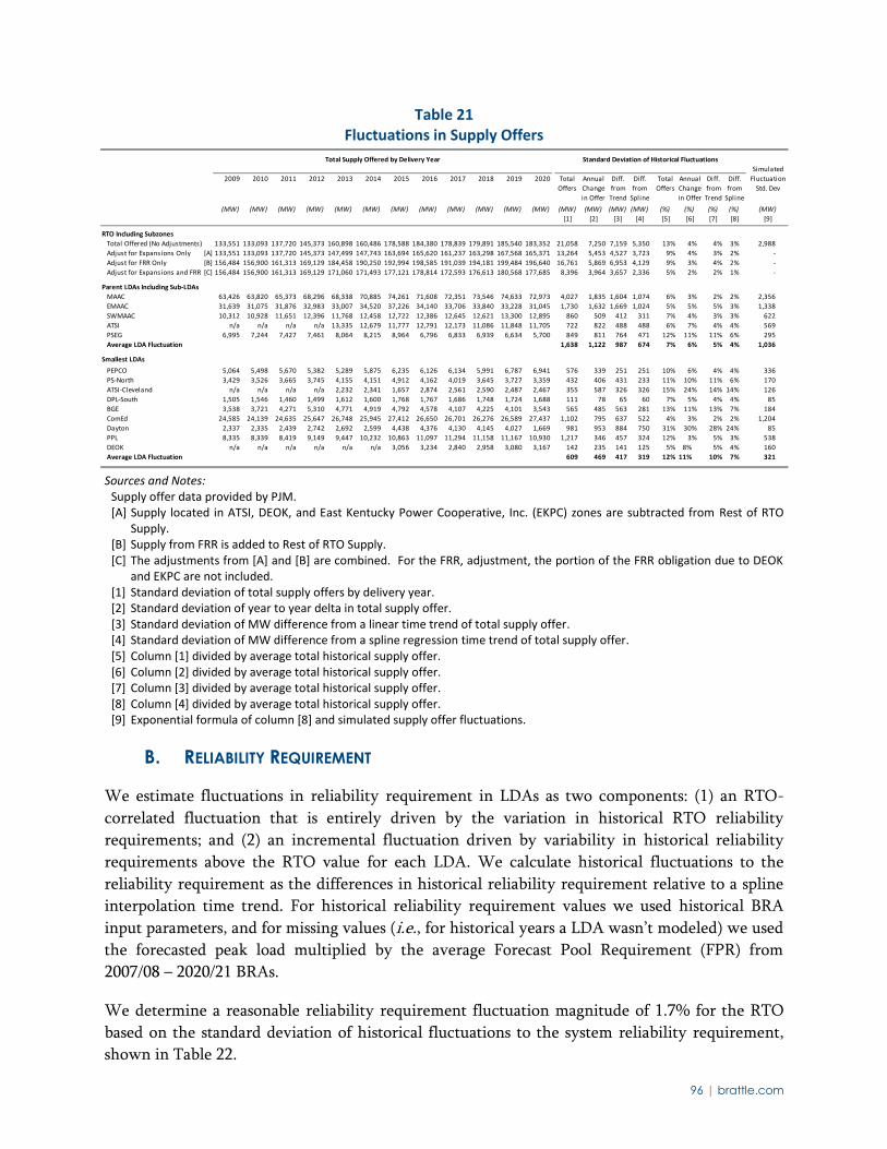
96 | brattle.com

Table 21 Fluctuations in Supply Offers

Sources and Notes: Supply offer data provided by PJM. [A] Supply located in ATSI, DEOK, and East Kentucky Power Cooperative, Inc. (EKPC) zones are subtracted from Rest of RTO

Supply. [B] Supply from FRR is added to Rest of RTO Supply. [C] The adjustments from [A] and [B] are combined. For the FRR, adjustment, the portion of the FRR obligation due to DEOK

and EKPC are not included. [1] Standard deviation of total supply offers by delivery year. [2] Standard deviation of year to year delta in total supply offer. [3] Standard deviation of MW difference from a linear time trend of total supply offer. [4] Standard deviation of MW difference from a spline regression time trend of total supply offer. [5] Column [1] divided by average total historical supply offer. [6] Column [2] divided by average total historical supply offer. [7] Column [3] divided by average total historical supply offer. [8] Column [4] divided by average total historical supply offer. [9] Exponential formula of column [8] and simulated supply offer fluctuations.

B. RELIABILITY REQUIREMENT

We estimate fluctuations in reliability requirement in LDAs as two components: (1) an RTO-

correlated fluctuation that is entirely driven by the variation in historical RTO reliability

requirements; and (2) an incremental fluctuation driven by variability in historical reliability

requirements above the RTO value for each LDA. We calculate historical fluctuations to the

reliability requirement as the differences in historical reliability requirement relative to a spline

interpolation time trend. For historical reliability requirement values we used historical BRA

input parameters, and for missing values (i.e., for historical years a LDA wasn’t modeled) we used

the forecasted peak load multiplied by the average Forecast Pool Requirement (FPR) from

2007/08 – 2020/21 BRAs.

We determine a reasonable reliability requirement fluctuation magnitude of 1.7% for the RTO

based on the standard deviation of historical fluctuations to the system reliability requirement,

shown in Table 22.

Total Supply Offered by Delivery Year Standard Deviation of Historical Fluctuations

Simulated

2009 2010 2011 2012 2013 2014 2015 2016 2017 2018 2019 2020 Total

Offers

Annual

Change

in Offer

Diff.

from

Trend

Diff.

from

Spline

Total

Offers

Annual

Change

in Offer

Diff.

from

Trend

Diff.

from

Spline

Fluctuation

Std. Dev

(MW) (MW) (MW) (MW) (MW) (MW) (MW) (MW) (MW) (MW) (MW) (MW) (MW) (MW) (MW) (MW) (%) (%) (%) (%) (MW)

[1] [2] [3] [4] [5] [6] [7] [8] [9]

RTO Including Subzones

Total Offered (No Adjustments) 133,551 133,093 137,720 145,373 160,898 160,486 178,588 184,380 178,839 179,891 185,540 183,352 21,058 7,250 7,159 5,350 13% 4% 4% 3% 2,988

Adjust for Expansions Only [A] 133,551 133,093 137,720 145,373 147,499 147,743 163,694 165,620 161,237 163,298 167,568 165,371 13,264 5,453 4,527 3,723 9% 4% 3% 2% -

Adjust for FRR Only [B] 156,484 156,900 161,313 169,129 184,458 190,250 192,994 198,585 191,039 194,181 199,484 196,640 16,761 5,869 6,953 4,129 9% 3% 4% 2% -

Adjust for Expansions and FRR [C] 156,484 156,900 161,313 169,129 171,060 171,493 177,121 178,814 172,593 176,613 180,568 177,685 8,396 3,964 3,657 2,336 5% 2% 2% 1% -

Parent LDAs Including Sub-LDAs

MAAC 63,426 63,820 65,373 68,296 68,338 70,885 74,261 71,608 72,351 73,546 74,633 72,973 4,027 1,835 1,604 1,074 6% 3% 2% 2% 2,356

EMAAC 31,639 31,075 31,876 32,983 33,007 34,520 37,226 34,140 33,706 33,840 33,228 31,045 1,730 1,632 1,669 1,024 5% 5% 5% 3% 1,338

SWMAAC 10,312 10,928 11,651 12,396 11,768 12,458 12,722 12,386 12,645 12,621 13,300 12,895 860 509 412 311 7% 4% 3% 3% 622

ATSI n/a n/a n/a n/a 13,335 12,679 11,777 12,791 12,173 11,086 11,848 11,705 722 822 488 488 6% 7% 4% 4% 569

PSEG 6,995 7,244 7,427 7,461 8,064 8,215 8,964 6,796 6,833 6,939 6,634 5,700 849 811 764 471 12% 11% 11% 6% 295

Average LDA Fluctuation 1,638 1,122 987 674 7% 6% 5% 4% 1,036

Smallest LDAs

PEPCO 5,064 5,498 5,670 5,382 5,289 5,875 6,235 6,126 6,134 5,991 6,787 6,941 576 339 251 251 10% 6% 4% 4% 336

PS-North 3,429 3,526 3,665 3,745 4,155 4,151 4,912 4,162 4,019 3,645 3,727 3,359 432 406 431 233 11% 10% 11% 6% 170

ATSI-Cleveland n/a n/a n/a n/a 2,232 2,341 1,657 2,874 2,561 2,590 2,487 2,467 355 587 326 326 15% 24% 14% 14% 126

DPL-South 1,505 1,546 1,460 1,499 1,612 1,600 1,768 1,767 1,686 1,748 1,724 1,688 111 78 65 60 7% 5% 4% 4% 85

BGE 3,538 3,721 4,271 5,310 4,771 4,919 4,792 4,578 4,107 4,225 4,101 3,543 565 485 563 281 13% 11% 13% 7% 184

ComEd 24,585 24,139 24,635 25,647 26,748 25,945 27,412 26,650 26,701 26,276 26,589 27,437 1,102 795 637 522 4% 3% 2% 2% 1,204

Dayton 2,337 2,335 2,439 2,742 2,692 2,599 4,438 4,376 4,130 4,145 4,027 1,669 981 953 884 750 31% 30% 28% 24% 85

PPL 8,335 8,339 8,419 9,149 9,447 10,232 10,863 11,097 11,294 11,158 11,167 10,930 1,217 346 457 324 12% 3% 5% 3% 538

DEOK n/a n/a n/a n/a n/a n/a 3,056 3,234 2,840 2,958 3,080 3,167 142 235 141 125 5% 8% 5% 4% 160

Average LDA Fluctuation 609 469 417 319 12% 11% 10% 7% 321

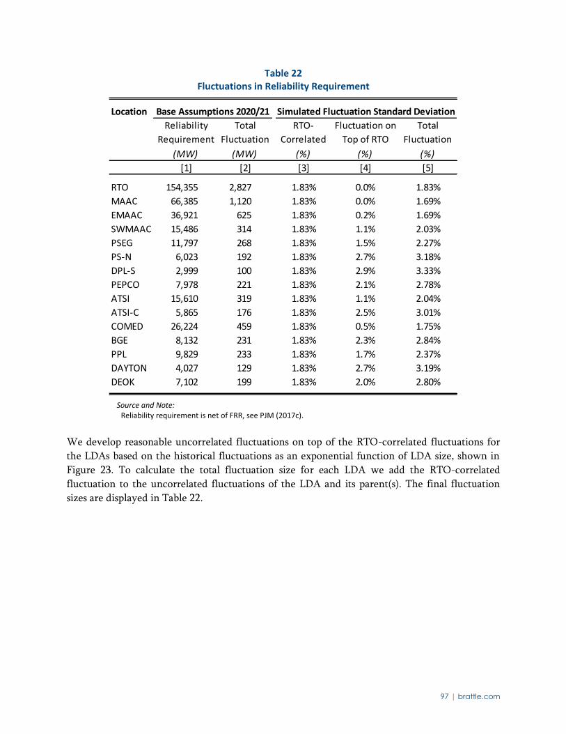
97 | brattle.com

Table 22 Fluctuations in Reliability Requirement

Source and Note: Reliability requirement is net of FRR, see PJM (2017c).

We develop reasonable uncorrelated fluctuations on top of the RTO-correlated fluctuations for

the LDAs based on the historical fluctuations as an exponential function of LDA size, shown in

Figure 23. To calculate the total fluctuation size for each LDA we add the RTO-correlated

fluctuation to the uncorrelated fluctuations of the LDA and its parent(s). The final fluctuation

sizes are displayed in Table 22.

Location Base Assumptions 2020/21 Simulated Fluctuation Standard Deviation

Reliability

Requirement

Total

Fluctuation

RTO-

Correlated

Shock

Fluctuation on

Top of RTO

Total

Fluctuation

(MW) (MW) (%) (%) (%)

[1] [2] [3] [4] [5]

RTO 154,355 2,827 1.83% 0.0% 1.83%

MAAC 66,385 1,120 1.83% 0.0% 1.69%

EMAAC 36,921 625 1.83% 0.2% 1.69%

SWMAAC 15,486 314 1.83% 1.1% 2.03%

PSEG 11,797 268 1.83% 1.5% 2.27%

PS-N 6,023 192 1.83% 2.7% 3.18%

DPL-S 2,999 100 1.83% 2.9% 3.33%

PEPCO 7,978 221 1.83% 2.1% 2.78%

ATSI 15,610 319 1.83% 1.1% 2.04%

ATSI-C 5,865 176 1.83% 2.5% 3.01%

COMED 26,224 459 1.83% 0.5% 1.75%

BGE 8,132 231 1.83% 2.3% 2.84%

PPL 9,829 233 1.83% 1.7% 2.37%

DAYTON 4,027 129 1.83% 2.7% 3.19%

DEOK 7,102 199 1.83% 2.0% 2.80%

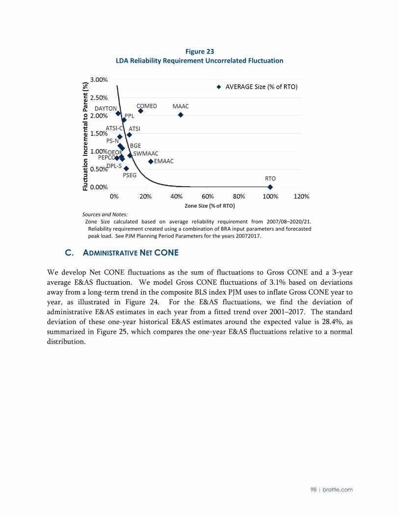
98 | brattle.com

Figure 23 LDA Reliability Requirement Uncorrelated Fluctuation

Sources and Notes:

Zone Size calculated based on average reliability requirement from 2007/08–2020/21. Reliability requirement created using a combination of BRA input parameters and forecasted peak load. See PJM Planning Period Parameters for the years 20072017.

C. ADMINISTRATIVE NET CONE

We develop Net CONE fluctuations as the sum of fluctuations to Gross CONE and a 3-year

average E&AS fluctuation. We model Gross CONE fluctuations of 3.1% based on deviations

away from a long-term trend in the composite BLS index PJM uses to inflate Gross CONE year to

year, as illustrated in Figure 24. For the E&AS fluctuations, we find the deviation of

administrative E&AS estimates in each year from a fitted trend over 2001–2017. The standard

deviation of these one-year historical E&AS estimates around the expected value is 28.4%, as

summarized in Figure 25, which compares the one-year E&AS fluctuations relative to a normal

distribution.

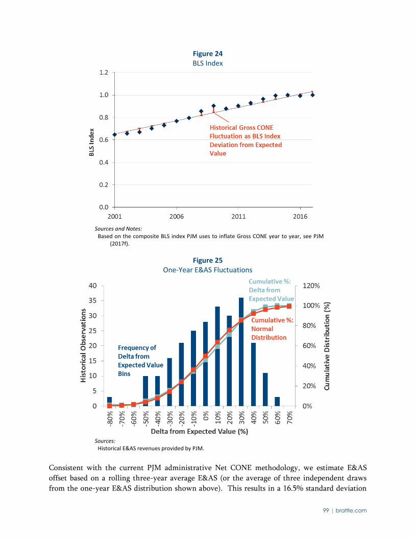
99 | brattle.com

Figure 24 BLS Index

Sources and Notes: Based on the composite BLS index PJM uses to inflate Gross CONE year to year, see PJM

(2017f).

Figure 25 One-Year E&AS Fluctuations

Sources: Historical E&AS revenues provided by PJM.

Consistent with the current PJM administrative Net CONE methodology, we estimate E&AS

offset based on a rolling three-year average E&AS (or the average of three independent draws

from the one-year E&AS distribution shown above). This results in a 16.5% standard deviation

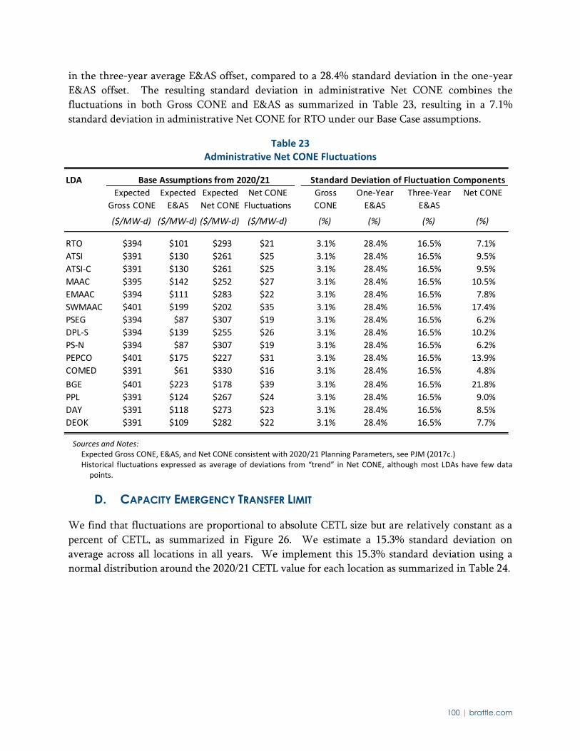
100 | brattle.com

in the three-year average E&AS offset, compared to a 28.4% standard deviation in the one-year

E&AS offset. The resulting standard deviation in administrative Net CONE combines the

fluctuations in both Gross CONE and E&AS as summarized in Table 23, resulting in a 7.1%

standard deviation in administrative Net CONE for RTO under our Base Case assumptions.

Table 23 Administrative Net CONE Fluctuations

Sources and Notes: Expected Gross CONE, E&AS, and Net CONE consistent with 2020/21 Planning Parameters, see PJM (2017c.) Historical fluctuations expressed as average of deviations from “trend” in Net CONE, although most LDAs have few data

points.

D. CAPACITY EMERGENCY TRANSFER LIMIT

We find that fluctuations are proportional to absolute CETL size but are relatively constant as a

percent of CETL, as summarized in Figure 26. We estimate a 15.3% standard deviation on

average across all locations in all years. We implement this 15.3% standard deviation using a

normal distribution around the 2020/21 CETL value for each location as summarized in Table 24.

LDA Base Assumptions from 2020/21 Standard Deviation of Fluctuation Components

Expected

Gross CONE

Expected

E&AS

Expected

Net CONE

Net CONE

Fluctuations

Gross

CONE

One-Year

E&AS

Three-Year

E&AS

Net CONE

($/MW-d) ($/MW-d) ($/MW-d) ($/MW-d) (%) (%) (%) (%)

RTO $394 $101 $293 $21 3.1% 28.4% 16.5% 7.1%

ATSI $391 $130 $261 $25 3.1% 28.4% 16.5% 9.5%

ATSI-C $391 $130 $261 $25 3.1% 28.4% 16.5% 9.5%

MAAC $395 $142 $252 $27 3.1% 28.4% 16.5% 10.5%

EMAAC $394 $111 $283 $22 3.1% 28.4% 16.5% 7.8%

SWMAAC $401 $199 $202 $35 3.1% 28.4% 16.5% 17.4%

PSEG $394 $87 $307 $19 3.1% 28.4% 16.5% 6.2%

DPL-S $394 $139 $255 $26 3.1% 28.4% 16.5% 10.2%

PS-N $394 $87 $307 $19 3.1% 28.4% 16.5% 6.2%

PEPCO $401 $175 $227 $31 3.1% 28.4% 16.5% 13.9%

COMED $391 $61 $330 $16 3.1% 28.4% 16.5% 4.8%

BGE $401 $223 $178 $39 3.1% 28.4% 16.5% 21.8%

PPL $391 $124 $267 $24 3.1% 28.4% 16.5% 9.0%

DAY $391 $118 $273 $23 3.1% 28.4% 16.5% 8.5%

DEOK $391 $109 $282 $22 3.1% 28.4% 16.5% 7.7%

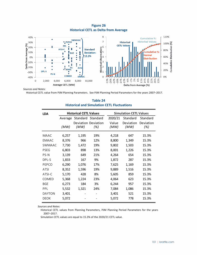
101 | brattle.com

Figure 26 Historical CETL as Delta from Average

Sources and Notes:

Historical CETL value from PJM Planning Parameters. See PJM Planning Period Parameters for the years 2007–2017.

Table 24 Historical and Simulation CETL Fluctuations

Sources and Notes: Historical CETL values from Planning Parameters, PJM Planning Period Parameters for the years

2007–2017. Simulation CETL values are equal to 15.3% of the 2020/21 CETL value.

LDA Historical CETL Values Simulation CETL Values

Average Standard

Deviation

Standard

Deviation

2020/21

Value

Standard

Deviation

Standard

Deviation(MW) (MW) (%) (MW) (MW) (%)

MAAC 6,257 1,195 19% 4,218 647 15.3%

EMAAC 8,376 966 12% 8,800 1,349 15.3%

SWMAAC 7,730 1,472 19% 9,802 1,503 15.3%

PSEG 6,803 898 13% 8,001 1,226 15.3%

PS-N 3,139 649 21% 4,264 654 15.3%

DPL-S 1,833 167 9% 1,872 287 15.3%

PEPCO 6,290 1,076 17% 7,625 1,169 15.3%

ATSI 8,352 1,596 19% 9,889 1,516 15.3%

ATSI-C 5,170 428 8% 5,605 859 15.3%

COMED 5,368 1,224 23% 4,064 623 15.3%

BGE 6,273 184 3% 6,244 957 15.3%

PPL 5,532 1,321 24% 7,084 1,086 15.3%

DAYTON 3,401 - - 3,401 521 15.3%

DEOK 5,072 - - 5,072 778 15.3%

E. NET SUPPLY

As discussed in Section III.E, the net supply comparison is the most important driver of price and

quantity in our model, as well as in historic market results. We calculate net supply fluctuations

as the supply plus CETL minus reliability requirement. All supply, CETL, reliability requirement

and net supply fluctuations are shown in Table 25. The simulated net supply fluctuations

generally fall between the simple standard deviation of historical values and the de-trended

values for the RTO and most LDAs, suggesting that they are a reasonable estimate.

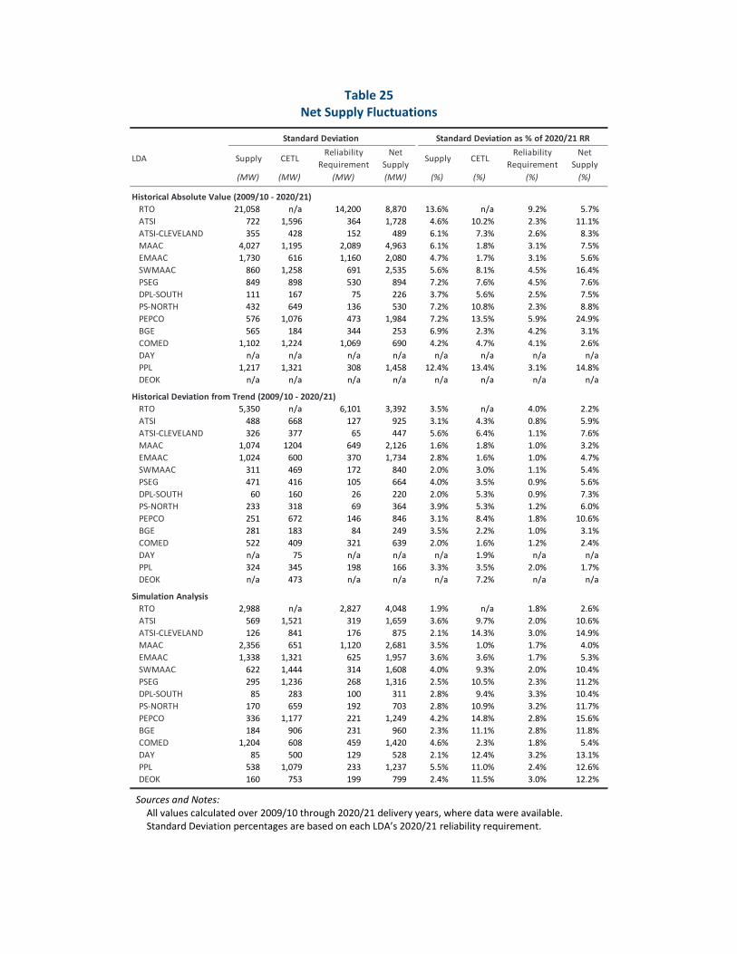
Table 25 Net Supply Fluctuations

Sources and Notes: All values calculated over 2009/10 through 2020/21 delivery years, where data were available. Standard Deviation percentages are based on each LDA’s 2020/21 reliability requirement.

Standard Deviation Standard Deviation as % of 2020/21 RR

LDA Supply CETLReliability

Requirement

Net

SupplySupply CETL

Reliability

Requirement

Net

Supply

(MW) (MW) (MW) (MW) (%) (%) (%) (%)

Historical Absolute Value (2009/10 - 2020/21)

RTO 21,058 n/a 14,200 8,870 13.6% n/a 9.2% 5.7%

ATSI 722 1,596 364 1,728 4.6% 10.2% 2.3% 11.1%

ATSI-CLEVELAND 355 428 152 489 6.1% 7.3% 2.6% 8.3%

MAAC 4,027 1,195 2,089 4,963 6.1% 1.8% 3.1% 7.5%

EMAAC 1,730 616 1,160 2,080 4.7% 1.7% 3.1% 5.6%

SWMAAC 860 1,258 691 2,535 5.6% 8.1% 4.5% 16.4%

PSEG 849 898 530 894 7.2% 7.6% 4.5% 7.6%

DPL-SOUTH 111 167 75 226 3.7% 5.6% 2.5% 7.5%

PS-NORTH 432 649 136 530 7.2% 10.8% 2.3% 8.8%

PEPCO 576 1,076 473 1,984 7.2% 13.5% 5.9% 24.9%

BGE 565 184 344 253 6.9% 2.3% 4.2% 3.1%

COMED 1,102 1,224 1,069 690 4.2% 4.7% 4.1% 2.6%

DAY n/a n/a n/a n/a n/a n/a n/a n/a

PPL 1,217 1,321 308 1,458 12.4% 13.4% 3.1% 14.8%

DEOK n/a n/a n/a n/a n/a n/a n/a n/a

Historical Deviation from Trend (2009/10 - 2020/21)

RTO 5,350 n/a 6,101 3,392 3.5% n/a 4.0% 2.2%

ATSI 488 668 127 925 3.1% 4.3% 0.8% 5.9%

ATSI-CLEVELAND 326 377 65 447 5.6% 6.4% 1.1% 7.6%

MAAC 1,074 1204 649 2,126 1.6% 1.8% 1.0% 3.2%

EMAAC 1,024 600 370 1,734 2.8% 1.6% 1.0% 4.7%

SWMAAC 311 469 172 840 2.0% 3.0% 1.1% 5.4%

PSEG 471 416 105 664 4.0% 3.5% 0.9% 5.6%

DPL-SOUTH 60 160 26 220 2.0% 5.3% 0.9% 7.3%

PS-NORTH 233 318 69 364 3.9% 5.3% 1.2% 6.0%

PEPCO 251 672 146 846 3.1% 8.4% 1.8% 10.6%

BGE 281 183 84 249 3.5% 2.2% 1.0% 3.1%

COMED 522 409 321 639 2.0% 1.6% 1.2% 2.4%

DAY n/a 75 n/a n/a n/a 1.9% n/a n/a

PPL 324 345 198 166 3.3% 3.5% 2.0% 1.7%

DEOK n/a 473 n/a n/a n/a 7.2% n/a n/a

Simulation Analysis

RTO 2,988 n/a 2,827 4,048 1.9% n/a 1.8% 2.6%

ATSI 569 1,521 319 1,659 3.6% 9.7% 2.0% 10.6%

ATSI-CLEVELAND 126 841 176 875 2.1% 14.3% 3.0% 14.9%

MAAC 2,356 651 1,120 2,681 3.5% 1.0% 1.7% 4.0%

EMAAC 1,338 1,321 625 1,957 3.6% 3.6% 1.7% 5.3%

SWMAAC 622 1,444 314 1,608 4.0% 9.3% 2.0% 10.4%

PSEG 295 1,236 268 1,316 2.5% 10.5% 2.3% 11.2%

DPL-SOUTH 85 283 100 311 2.8% 9.4% 3.3% 10.4%

PS-NORTH 170 659 192 703 2.8% 10.9% 3.2% 11.7%

PEPCO 336 1,177 221 1,249 4.2% 14.8% 2.8% 15.6%

BGE 184 906 231 960 2.3% 11.1% 2.8% 11.8%

COMED 1,204 608 459 1,420 4.6% 2.3% 1.8% 5.4%

DAY 85 500 129 528 2.1% 12.4% 3.2% 13.1%

PPL 538 1,079 233 1,237 5.5% 11.0% 2.4% 12.6%

DEOK 160 753 199 799 2.4% 11.5% 3.0% 12.2%

Appendix B: Supply Curves with Capacity Performance

Under Capacity Performance, resources that do not fulfill their capacity obligation during

emergency events are penalized, while resources that perform over their obligation are awarded

bonus payments.86 Resources that do not have a capacity obligation are eligible for bonuses on

their full output during emergency events, while resources with obligations are only eligible for

bonuses on their output in excess of their obligation. Figure 27 summarizes Capacity

Performance penalties and bonuses to resources with and without an obligation.

Figure 27 Capacity Performance Penalties and Bonuses

Sources: See PJM (2017h), OATT Attachment DD.10.

As discussed in Section III.C, the 2020/21 BRA was the first auction where only Capacity

Performance resources were procured.87 It is important in the context of this review because of

how we model supply and the effect of Capacity Performance on the supply curve shape. As we

saw in Figure 13, the implementation of Capacity Performance has reduced the number of zero-

priced offers and flattened the lower part of the supply curve during the Capacity Performance

BRAs compared to the pre-Capacity Performance BRAs.

86 Bonus payments are funded by the penalty payments charged to non-performing resources.

87 2018/19 and 2019/20 were transition years where Capacity Performance and base resources were both

procured.

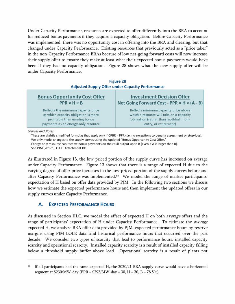
Under Capacity Performance, resources are expected to offer differently into the BRA to account

for reduced bonus payments if they acquire a capacity obligation. Before Capacity Performance

was implemented, there was no opportunity cost in offering into the BRA and clearing, but that

changed under Capacity Performance. Existing resources that previously acted as a “price taker”

in the non-Capacity Performance BRAs because of low net-going forward costs will now increase

their supply offer to ensure they make at least what their expected bonus payments would have

been if they had no capacity obligation. Figure 28 shows what the new supply offer will be

under Capacity Performance.

Figure 28 Adjusted Supply Offer under Capacity Performance

Sources and Notes: These are slightly simplified formulas that apply only if CPBR = PPR (i.e. no exceptions to penalty assessment or stop-loss). We only model changes to the supply curves using the updated “Bonus Opportunity Cost Offer.” Energy-only resource can receive bonus payments on their full output up to B (even if A is larger than B). See PJM (2017h), OATT Attachment DD.

As illustrated in Figure 13, the low-priced portion of the supply curve has increased on average

under Capacity Performance. Figure 13 shows that there is a range of expected H due to the

varying degree of offer price increases in the low-priced portion of the supply curves before and

after Capacity Performance was implemented.88 We model the range of market participants’

expectation of H based on offer data provided by PJM. In the following two sections we discuss

how we estimate the expected performance hours and then implement the updated offers in our

supply curves under Capacity Performance.

A. EXPECTED PERFORMANCE HOURS

As discussed in Section III.C, we model the effect of expected H on both average offers and the

range of participants’ expectation of H under Capacity Performance. To estimate the average

expected H, we analyze BRA offer data provided by PJM, expected performance hours by reserve

margins using PJM LOLE data, and historical performance hours that occurred over the past

decade. We consider two types of scarcity that lead to performance hours: installed capacity

scarcity and operational scarcity. Installed capacity scarcity is a result of installed capacity falling

below a threshold supply buffer above load. Operational scarcity is a result of plants not

88 If all participants had the same expected H, the 2020/21 BRA supply curve would have a horizontal

segment at $230/MW-day (PPR = $293/MW-day ÷ 30, H = 30, B = 78.5%).

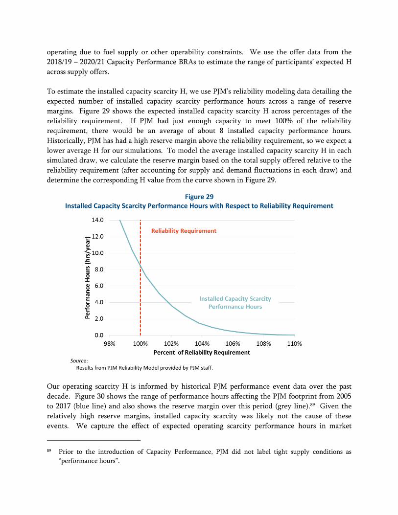
operating due to fuel supply or other operability constraints. We use the offer data from the

2018/19 – 2020/21 Capacity Performance BRAs to estimate the range of participants’ expected H

across supply offers.

To estimate the installed capacity scarcity H, we use PJM’s reliability modeling data detailing the

expected number of installed capacity scarcity performance hours across a range of reserve

margins. Figure 29 shows the expected installed capacity scarcity H across percentages of the

reliability requirement. If PJM had just enough capacity to meet 100% of the reliability

requirement, there would be an average of about 8 installed capacity performance hours.

Historically, PJM has had a high reserve margin above the reliability requirement, so we expect a

lower average H for our simulations. To model the average installed capacity scarcity H in each

simulated draw, we calculate the reserve margin based on the total supply offered relative to the

reliability requirement (after accounting for supply and demand fluctuations in each draw) and

determine the corresponding H value from the curve shown in Figure 29.

Figure 29 Installed Capacity Scarcity Performance Hours with Respect to Reliability Requirement

Source:

Results from PJM Reliability Model provided by PJM staff.

Our operating scarcity H is informed by historical PJM performance event data over the past

decade. Figure 30 shows the range of performance hours affecting the PJM footprint from 2005

to 2017 (blue line) and also shows the reserve margin over this period (grey line).89 Given the

relatively high reserve margins, installed capacity scarcity was likely not the cause of these

events. We capture the effect of expected operating scarcity performance hours in market

89 Prior to the introduction of Capacity Performance, PJM did not label tight supply conditions as

“performance hours”.

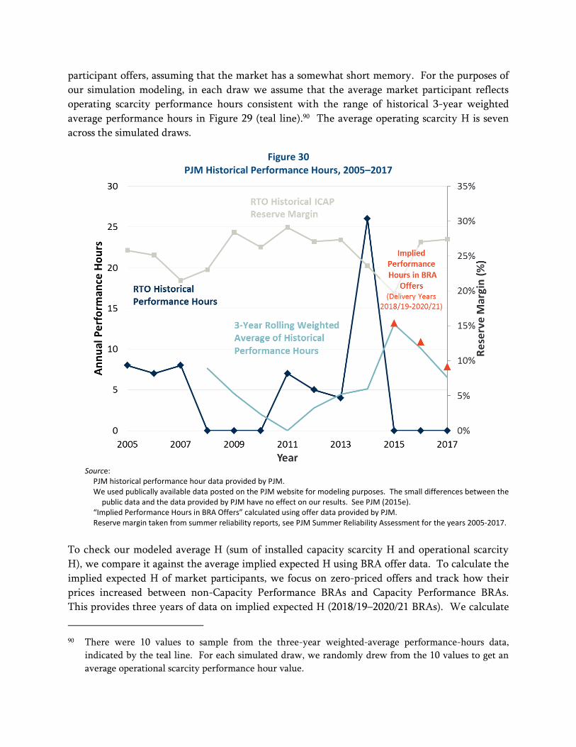
participant offers, assuming that the market has a somewhat short memory. For the purposes of

our simulation modeling, in each draw we assume that the average market participant reflects

operating scarcity performance hours consistent with the range of historical 3-year weighted

average performance hours in Figure 29 (teal line).90 The average operating scarcity H is seven

across the simulated draws.

Figure 30 PJM Historical Performance Hours, 2005–2017

Source:

PJM historical performance hour data provided by PJM. We used publically available data posted on the PJM website for modeling purposes. The small differences between the

public data and the data provided by PJM have no effect on our results. See PJM (2015e). “Implied Performance Hours in BRA Offers” calculated using offer data provided by PJM. Reserve margin taken from summer reliability reports, see PJM Summer Reliability Assessment for the years 2005-2017.

To check our modeled average H (sum of installed capacity scarcity H and operational scarcity

H), we compare it against the average implied expected H using BRA offer data. To calculate the

implied expected H of market participants, we focus on zero-priced offers and track how their

prices increased between non-Capacity Performance BRAs and Capacity Performance BRAs.

This provides three years of data on implied expected H (2018/19–2020/21 BRAs). We calculate

90 There were 10 values to sample from the three-year weighted-average performance-hours data,

indicated by the teal line. For each simulated draw, we randomly drew from the 10 values to get an

average operational scarcity performance hour value.

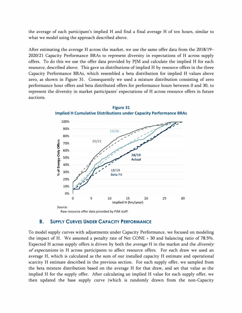
the average of each participant’s implied H and find a final average H of ten hours, similar to

what we model using the approach described above.

After estimating the average H across the market, we use the same offer data from the 2018/19–

2020/21 Capacity Performance BRAs to represent diversity in expectations of H across supply

offers. To do this we use the offer data provided by PJM and calculate the implied H for each

resource, described above. This gave us distributions of implied H by resource offers in the three

Capacity Performance BRAs, which resembled a beta distribution for implied H values above

zero, as shown in Figure 31. Consequently we used a mixture distribution consisting of zero

performance hour offers and beta distributed offers for performance hours between 0 and 30, to

represent the diversity in market participants’ expectations of H across resource offers in future

auctions.

Figure 31 Implied H Cumulative Distributions under Capacity Performance BRAs

Source:

Raw resource offer data provided by PJM staff.

B. SUPPLY CURVES UNDER CAPACITY PERFORMANCE

To model supply curves with adjustments under Capacity Performance, we focused on modeling

the impact of H. We assumed a penalty rate of Net CONE ÷ 30 and balancing ratio of 78.5%.

Expected H across supply offers is driven by both the average H in the market and the diversity of expectations in H across participants to affect resource offers. For each draw we used an

average H, which is calculated as the sum of our installed capacity H estimate and operational

scarcity H estimate described in the previous section. For each supply offer, we sampled from

the beta mixture distribution based on the average H for that draw, and set that value as the

implied H for the supply offer. After calculating an implied H value for each supply offer, we

then updated the base supply curve (which is randomly drawn from the non-Capacity

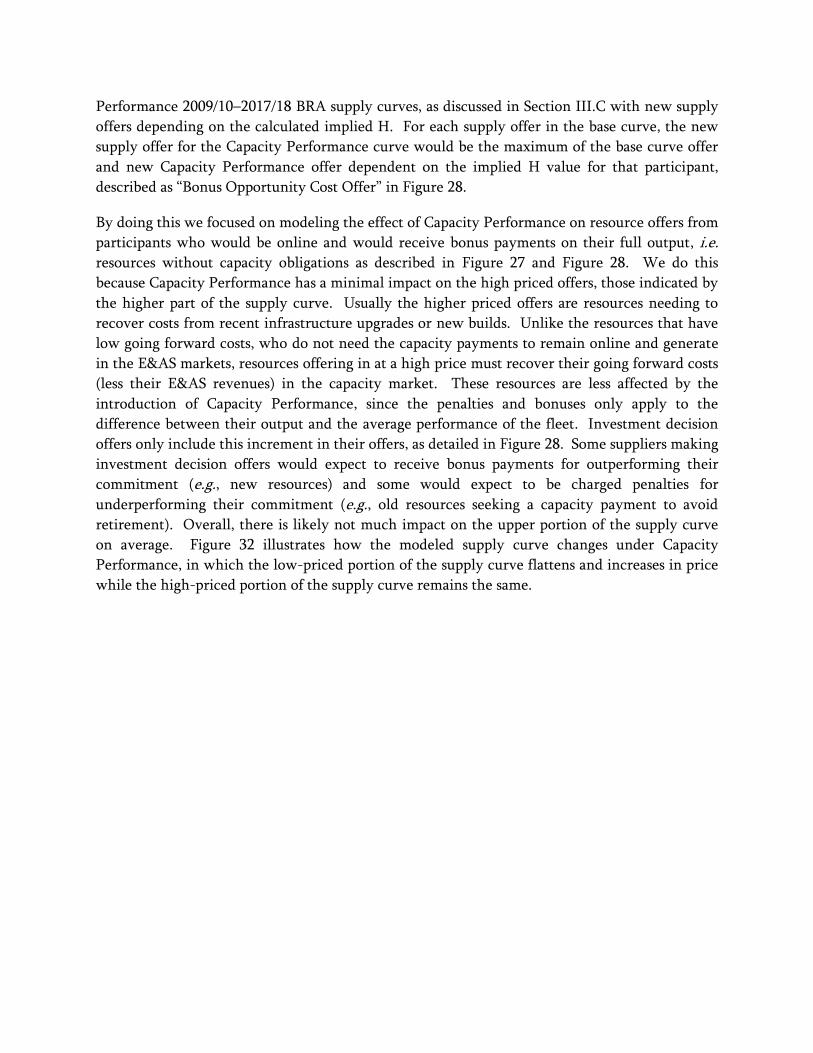
Performance 2009/10–2017/18 BRA supply curves, as discussed in Section III.C with new supply

offers depending on the calculated implied H. For each supply offer in the base curve, the new

supply offer for the Capacity Performance curve would be the maximum of the base curve offer

and new Capacity Performance offer dependent on the implied H value for that participant,

described as “Bonus Opportunity Cost Offer” in Figure 28.

By doing this we focused on modeling the effect of Capacity Performance on resource offers from

participants who would be online and would receive bonus payments on their full output, i.e. resources without capacity obligations as described in Figure 27 and Figure 28. We do this

because Capacity Performance has a minimal impact on the high priced offers, those indicated by

the higher part of the supply curve. Usually the higher priced offers are resources needing to

recover costs from recent infrastructure upgrades or new builds. Unlike the resources that have

low going forward costs, who do not need the capacity payments to remain online and generate

in the E&AS markets, resources offering in at a high price must recover their going forward costs

(less their E&AS revenues) in the capacity market. These resources are less affected by the

introduction of Capacity Performance, since the penalties and bonuses only apply to the

difference between their output and the average performance of the fleet. Investment decision

offers only include this increment in their offers, as detailed in Figure 28. Some suppliers making

investment decision offers would expect to receive bonus payments for outperforming their

commitment (e.g., new resources) and some would expect to be charged penalties for

underperforming their commitment (e.g., old resources seeking a capacity payment to avoid

retirement). Overall, there is likely not much impact on the upper portion of the supply curve

on average. Figure 32 illustrates how the modeled supply curve changes under Capacity

Performance, in which the low-priced portion of the supply curve flattens and increases in price

while the high-priced portion of the supply curve remains the same.

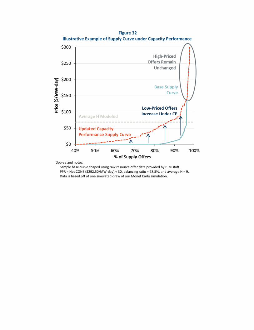
Figure 32 Illustrative Example of Supply Curve under Capacity Performance

Source and notes:

Sample base curve shaped using raw resource offer data provided by PJM staff. PPR = Net CONE ($292.50/MW-day) ÷ 30, balancing ratio = 78.5%, and average H = 9. Data is based off of one simulated draw of our Monet Carlo simulation.

Documents

Fourth Review of PJM’s Variable