FOURTH ORDER TIME-STEPPING FORKADOMTSEV-PETVIASHVILI AND DAVEY-STEWARTSON

EQUATIONS∗

C. KLEIN† AND K. ROIDOT‡

Abstract. Purely dispersive partial differential equations as the Korteweg-de Vries equation,the nonlinear Schrodinger equation and higher dimensional generalizations thereof can have solu-tions which develop a zone of rapid modulated oscillations in the region where the correspondingdispersionless equations have shocks or blow-up. To numerically study such phenomena, fourthorder time-stepping in combination with spectral methods is beneficial to resolve the steep gradi-ents in the oscillatory region. We compare the performance of several fourth order methods forthe Kadomtsev-Petviashvili and the Davey-Stewartson equations, two integrable equations in 2+1dimensions: exponential time-differencing, integrating factors, time-splitting, implicit Runge-Kuttaand Driscoll’s IMEX method. The accuracy in the numerical conservation of integrals of motion isdiscussed.

Key words. Exponential Time-Differencing, Kadomtsev-Petviashvili equation, Davey-Stewartsonsystems, split step, integrating factor method, implicit explicit schemes, dispersive shocks

AMS subject classifications. Primary, 65M70; Secondary, 65L05, 65M20

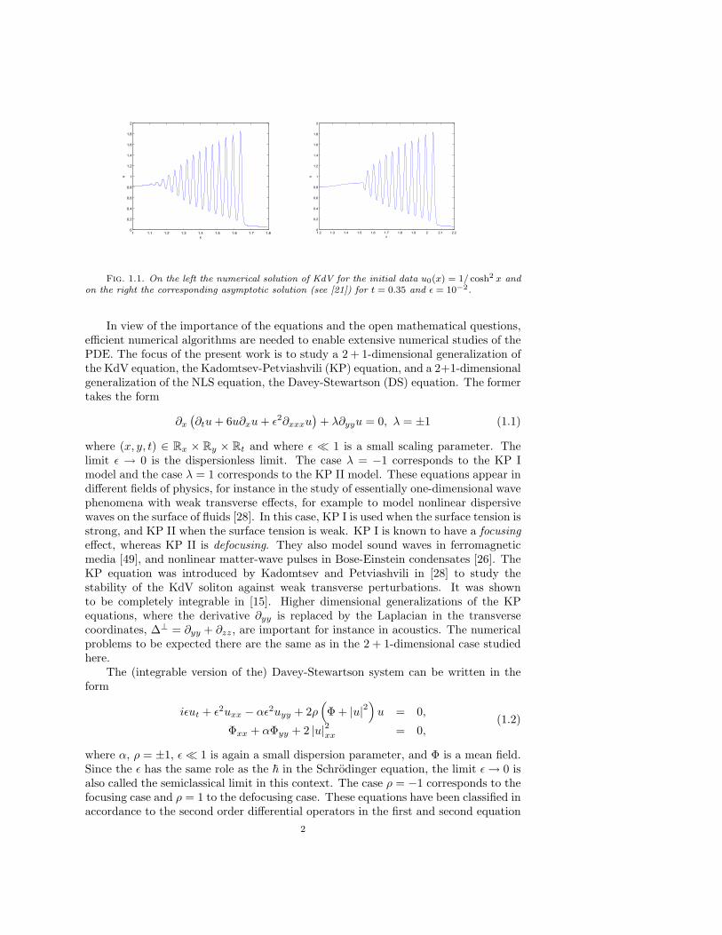
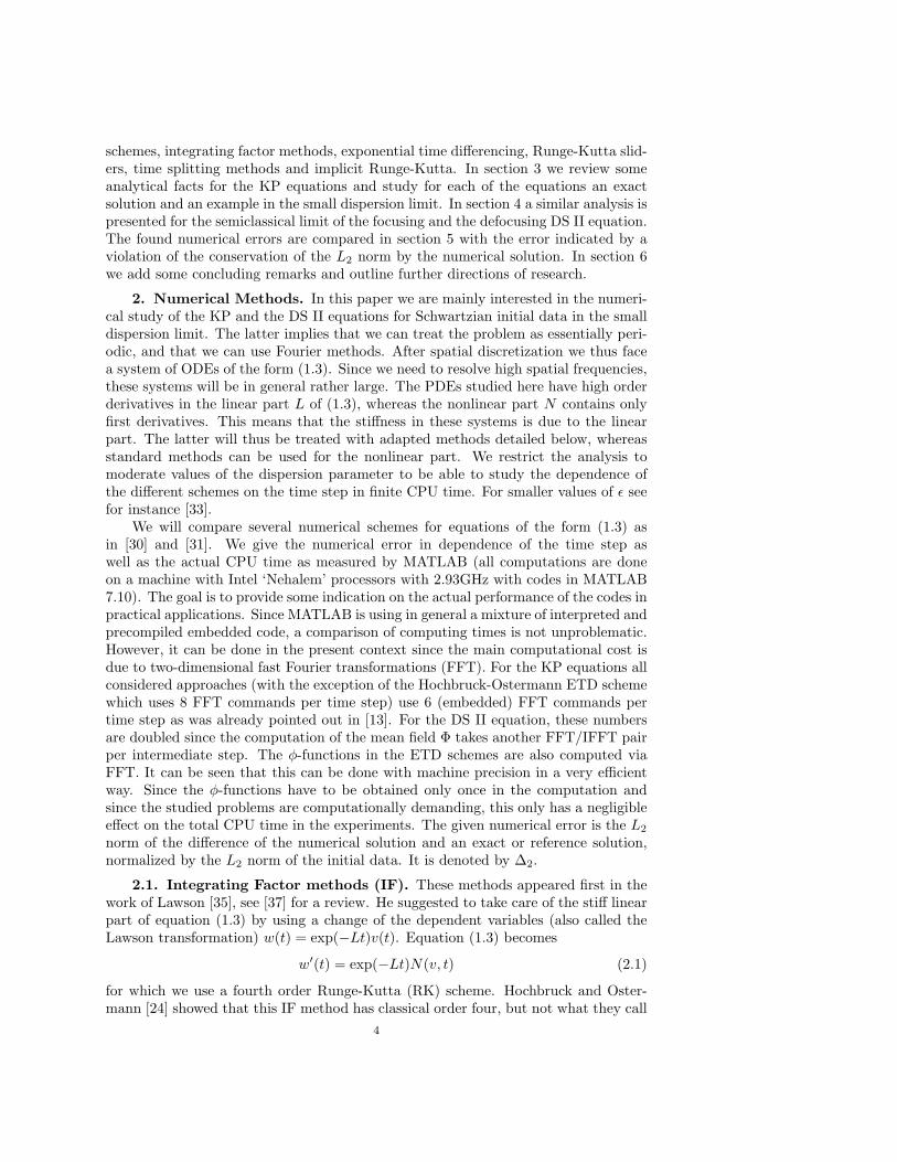
1. Introduction. Nonlinear dispersive partial differential equations (PDE) playan important role in applications since they appear in many approximations to systemsin hydrodynamics, nonlinear optics, acoustics, plasma physics, Bose-Einstein conden-sates. . . The most prominent members of the class are the celebrated Korteweg-deVries (KdV) equation and the nonlinear Schrodinger (NLS) equation and higher di-mensional generalizations of these. In addition to the importance of these equationsin applications, there is also a considerable interest in the mathematical propertiesof their solutions. It is known that nonlinear dispersive PDE without dissipation canhave dispersive shock waves [22], i.e., regions of rapid modulated oscillations in thevicinity of shocks in the solutions to the corresponding dispersionless equations forthe same initial data. Thus solutions to dispersive PDE in general will not have astrong dispersionless limit as known from solutions to dissipative PDE as the Burg-ers’ equation in the limit of vanishing dissipation. An asymptotic description of thesedispersive shocks is known for certain integrable PDE as KdV [36, 50, 11] and theNLS equation for classes of initial data [27, 29, 47]. For KdV an example is shown inFig. 1.1, for details see [21].

No such description is known for 2 + 1-dimensional PDE. In addition solutionsto nonlinear dispersive PDE can have blowup, i.e., a loss of regularity of the solutionwith respect to the initial data. It is known for many of the PDE under considerationwhen blowup can occur, but for the precise mechanism of the blowup often not evenconjectures exist.

∗We thank P. Matthews, B. Muite, A. Ostermann, T. Schmelzer, who provided example codes,and L.N. Trefethen, who interested us in the subject, for helpful discussion and hints. This work hasbeen supported by the project FroM-PDE funded by the European Research Council through theAdvanced Investigator Grant Scheme, the Conseil Regional de Bourgogne via a FABER grant andthe ANR via the program ANR-09-BLAN-0117-01.†Institut de Mathematiques de Bourgogne, Universite de Bourgogne, 9 avenue Alain Savary, 21078

Dijon Cedex, France (christian.klein@u-bourgogne.fr)‡Institut de Mathematiques de Bourgogne, Universite de Bourgogne, 9 avenue Alain Savary, 21078

Dijon Cedex, France (kristelle.roidot@u-bourgogne.fr)

1

1 1.1 1.2 1.3 1.4 1.5 1.6 1.7 1.80

0.2

0.4

0.6

0.8

1

1.2

1.4

1.6

1.8

2

x

u

1.2 1.3 1.4 1.5 1.6 1.7 1.8 1.9 2 2.1 2.20

0.2

0.4

0.6

0.8

1

1.2

1.4

1.6

1.8

2

x

u

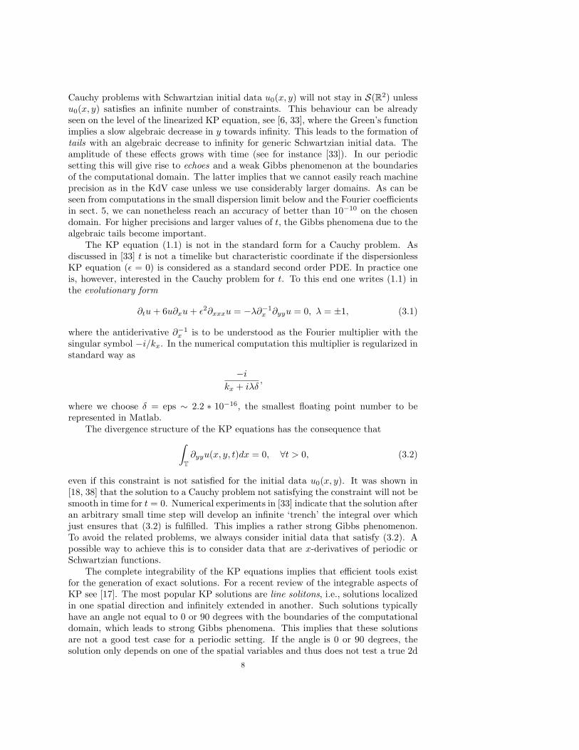
Fig. 1.1. On the left the numerical solution of KdV for the initial data u0(x) = 1/ cosh2 x andon the right the corresponding asymptotic solution (see [21]) for t = 0.35 and ε = 10−2.

In view of the importance of the equations and the open mathematical questions,efficient numerical algorithms are needed to enable extensive numerical studies of thePDE. The focus of the present work is to study a 2 + 1-dimensional generalization ofthe KdV equation, the Kadomtsev-Petviashvili (KP) equation, and a 2+1-dimensionalgeneralization of the NLS equation, the Davey-Stewartson (DS) equation. The formertakes the form

∂x(∂tu+ 6u∂xu+ ε2∂xxxu

)+ λ∂yyu = 0, λ = ±1 (1.1)

where (x, y, t) ∈ Rx × Ry × Rt and where ε � 1 is a small scaling parameter. Thelimit ε → 0 is the dispersionless limit. The case λ = −1 corresponds to the KP Imodel and the case λ = 1 corresponds to the KP II model. These equations appear indifferent fields of physics, for instance in the study of essentially one-dimensional wavephenomena with weak transverse effects, for example to model nonlinear dispersivewaves on the surface of fluids [28]. In this case, KP I is used when the surface tension isstrong, and KP II when the surface tension is weak. KP I is known to have a focusingeffect, whereas KP II is defocusing. They also model sound waves in ferromagneticmedia [49], and nonlinear matter-wave pulses in Bose-Einstein condensates [26]. TheKP equation was introduced by Kadomtsev and Petviashvili in [28] to study thestability of the KdV soliton against weak transverse perturbations. It was shownto be completely integrable in [15]. Higher dimensional generalizations of the KPequations, where the derivative ∂yy is replaced by the Laplacian in the transversecoordinates, ∆⊥ = ∂yy + ∂zz, are important for instance in acoustics. The numericalproblems to be expected there are the same as in the 2 + 1-dimensional case studiedhere.

The (integrable version of the) Davey-Stewartson system can be written in theform

iεut + ε2uxx − αε2uyy + 2ρ(

Φ + |u|2)u = 0,

Φxx + αΦyy + 2 |u|2xx = 0,(1.2)

where α, ρ = ±1, ε� 1 is again a small dispersion parameter, and Φ is a mean field.Since the ε has the same role as the ~ in the Schrodinger equation, the limit ε→ 0 isalso called the semiclassical limit in this context. The case ρ = −1 corresponds to thefocusing case and ρ = 1 to the defocusing case. These equations have been classified inaccordance to the second order differential operators in the first and second equation

2

of (1.2). The hyperbolic-elliptic case [20] is known as DS II, whereas DS I is theelliptic-hyperbolic case. Both systems are completely integrable [1]. In the following,we will only consider the case DS II (α = 1) since the mean field Φ is then obtainedby inverting an elliptic operator. These DS systems model the evolution of weaklynonlinear water waves that travel predominantly in one direction, but in which thewave amplitude is modulated slowly in two horizontal directions [10], [12]. They arealso used in plasma physics [39, 40], to describe the evolution of a plasma under theaction of a magnetic field.

Since both KP and DS are completely integrable, there exist many explicit solu-tions, which thus provide popular test cases for numerical algorithms. But as we willshow at the example of KP, these exact solutions, typically solitons, often test theequation in a non-stiff regime. The main challenge in the study of critical phenom-ena as dispersive shocks and blowups is, however, the numerical resolution of stronggradients in the presence of which the above equations are stiff. This implies thatalgorithms that perform well for solitons might not be efficient in the context studiedhere.

Since critical phenomena are generally believed to be independent of the chosenboundary conditions, we study a periodic setting. Such settings also include rapidlydecreasing functions which can be periodically continued within the finite numericalprecision. This allows to approximate the spatial dependence via truncated Fourierseries which leads for the studied equations to large stiff systems of ODEs, see below.The use of Fourier methods not only gives spectral accuracy in the spatial coordinates,but also minimizes the introduction of numerical dissipation which is important inthe study of dispersive effects. In Fourier space, equations (1.1) and (1.2) have theform

vt = Lv + N(v, t), (1.3)

where v denotes the (discrete) Fourier transform of u, and where L and N denote linearand nonlinear operators, respectively. The resulting systems of ODEs are classicalexamples of stiff equations where the stiffness is related to the linear part L (it is aconsequence of the distribution of the eigenvalues of L), whereas the nonlinear partcontains only low order derivatives. In the small dispersion limit, this stiffness is stillpresent despite the small term ε2 in L. This is due to the fact that the smaller ε, thehigher spatial frequencies are needed to resolve the rapid oscillations.

There are several approaches to deal efficiently with equations of the form (1.3)with a linear stiff part as implicit-explicit (IMEX), time splitting, integrating factor(IF), and deferred correction schemes as well as sliders and exponential time differ-encing. To avoid as much as possible a pollution of the Fourier coefficients by errorsdue to the finite difference schemes for the time integration and to allow for largertime steps, we only consider fourth order schemes. While standard explicit schemesimpose prohibitively small time steps due to stability requirements (for the studiedexamples the standard fourth order Runge-Kutta (RK) scheme did not converge forthe used time steps), stable implicit schemes are in general computationally too ex-pensive in 2 + 1 dimensions. As an example of the latter we consider an implicitfourth order Runge-Kutta scheme. The focus of this paper is, however, to comparethe performance of several explicit fourth order schemes mainly related to exponen-tial integrators for various examples in a similar way as in the work by Kassam andTrefethen [30] and in [31] for KdV and NLS.

The paper is organized as follows: In section 2 we briefly list the used numerical3

schemes, integrating factor methods, exponential time differencing, Runge-Kutta slid-ers, time splitting methods and implicit Runge-Kutta. In section 3 we review someanalytical facts for the KP equations and study for each of the equations an exactsolution and an example in the small dispersion limit. In section 4 a similar analysis ispresented for the semiclassical limit of the focusing and the defocusing DS II equation.The found numerical errors are compared in section 5 with the error indicated by aviolation of the conservation of the L2 norm by the numerical solution. In section 6we add some concluding remarks and outline further directions of research.

2. Numerical Methods. In this paper we are mainly interested in the numeri-cal study of the KP and the DS II equations for Schwartzian initial data in the smalldispersion limit. The latter implies that we can treat the problem as essentially peri-odic, and that we can use Fourier methods. After spatial discretization we thus facea system of ODEs of the form (1.3). Since we need to resolve high spatial frequencies,these systems will be in general rather large. The PDEs studied here have high orderderivatives in the linear part L of (1.3), whereas the nonlinear part N contains onlyfirst derivatives. This means that the stiffness in these systems is due to the linearpart. The latter will thus be treated with adapted methods detailed below, whereasstandard methods can be used for the nonlinear part. We restrict the analysis tomoderate values of the dispersion parameter to be able to study the dependence ofthe different schemes on the time step in finite CPU time. For smaller values of ε seefor instance [33].

We will compare several numerical schemes for equations of the form (1.3) asin [30] and [31]. We give the numerical error in dependence of the time step aswell as the actual CPU time as measured by MATLAB (all computations are doneon a machine with Intel ‘Nehalem’ processors with 2.93GHz with codes in MATLAB7.10). The goal is to provide some indication on the actual performance of the codes inpractical applications. Since MATLAB is using in general a mixture of interpreted andprecompiled embedded code, a comparison of computing times is not unproblematic.However, it can be done in the present context since the main computational cost isdue to two-dimensional fast Fourier transformations (FFT). For the KP equations allconsidered approaches (with the exception of the Hochbruck-Ostermann ETD schemewhich uses 8 FFT commands per time step) use 6 (embedded) FFT commands pertime step as was already pointed out in [13]. For the DS II equation, these numbersare doubled since the computation of the mean field Φ takes another FFT/IFFT pairper intermediate step. The φ-functions in the ETD schemes are also computed viaFFT. It can be seen that this can be done with machine precision in a very efficientway. Since the φ-functions have to be obtained only once in the computation andsince the studied problems are computationally demanding, this only has a negligibleeffect on the total CPU time in the experiments. The given numerical error is the L2

norm of the difference of the numerical solution and an exact or reference solution,normalized by the L2 norm of the initial data. It is denoted by ∆2.

2.1. Integrating Factor methods (IF). These methods appeared first in thework of Lawson [35], see [37] for a review. He suggested to take care of the stiff linearpart of equation (1.3) by using a change of the dependent variables (also called theLawson transformation) w(t) = exp(−Lt)v(t). Equation (1.3) becomes

w′(t) = exp(−Lt)N(v, t) (2.1)

for which we use a fourth order Runge-Kutta (RK) scheme. Hochbruck and Oster-mann [24] showed that this IF method has classical order four, but not what they call

4

stiff order four. Loosely speaking there will be additional contributions to the errorof much lower order in the time step in the stiff regime, i.e., in the case of large norm||L|| in the integrating factor. They could show that the scheme used here is only offirst order for semilinear parabolic problems in the stiff regime. An extension of thistheory to hyperbolic equations does not exist yet, but the results in [4], [31] indicatethat a similar behavior is to be expected for hyperbolic equations (both KP and DSare hyperbolic in the sense that the matrix L appearing in (1.3) has purely imaginaryeigenvalues).

2.2. Driscoll’s IMEX Method. The idea of IMEX methods (see e.g. [8] forKdV) is the use of a stable implicit method for the linear part of the equation (1.3)and an explicit scheme for the nonlinear part which is assumed to be non-stiff. In [30]such schemes did not perform satisfactorily for dispersive PDEs which is why we onlyconsider a more sophisticated variant here. Fornberg and Driscoll [14] provided aninteresting generalization of IMEX by splitting also the linear part of the equation inFourier space into regimes of high, medium, and low frequencies, and by using adaptednumerical schemes in each of them. They considered the NLS equation as an example.Driscoll’s [13] idea was to split the linear part of the equation in Fourier space justin regimes of high and low frequencies. He used the fourth order RK integrator forthe low frequencies and the lineary implicit RK method of order three for the highfrequencies. He showed that this method is in practice of fourth order over a widerange of step sizes. We confirm this here for the cases where the method converges,which it fails to do, however, sometimes in the stiff regime. In particular, he used thismethod for the KP II equation at the two phase solution we will also discuss in thispaper as a test case.

2.3. Exponential Time Differencing Methods. Exponential time differenc-ing schemes were developed originally by Certaine [7] in the 60s, see [37] and [25]for comprehensive reviews of ETD methods and their history. The basic idea is touse equidistant time steps h and to integrate equation (1.3) exactly between the timesteps tn and tn+1 with respect to t. With v(tn) = vn and v(tn+1) = vn+1, we get

vn+1 = eLhvn +∫ h

0

dτeL(h−τ)N(v(tn + τ), tn + τ).

The integral will be computed in an approximate way for which different schemesexist. We use here only Runge-Kutta schemes of classical order 4, Cox-Matthews[9], Krogstad [34] and Hochbruck-Ostermann [24]. The latter showed that the stifforder of the Cox-Matthews scheme is only two, and the one of Krogstad’s is three.Both are, however, three step methods, whereas the Hochbruck-Ostermann methodis a four step method that has stiff order four. Thus all these methods should showthe same convergence rate in the non-stiff regime, but are expected to differ in thestiff regime. Notice that these results [24] were established for parabolic PDE, andthat the applicability for hyperbolic PDE of the type studied here is not obvious.One of the purposes of our study is to get some experimental insight whether theHochbruck-Ostermann theory holds also in this case.

The main technical problem in the use of ETD schemes is the efficient and accuratenumerical evaluation of the functions

φi(z) =1

(i− 1)!

∫ 1

0

e(1−τ)zτ i−1, i = 1, 2, 3, 4,

5

i.e., functions of the form (ez−1)/z where one has to avoid cancellation errors. Kassamand Trefethen [30] used complex contour integrals to compute these functions. Theapproach is straight forward for diagonal operators L that occur here because of theuse of Fourier methods: one considers a unit circle around each point z and computesthe contour integral with the trapezoid rule which is known to be a spectral methodin this case. Schmelzer [42] made this approach more efficient by using the complexcontour approach only for values of z close to the pole, e.g with |z| < 1/2. For thesame values of z the functions φi can be computed via a Taylor series. These twoindependent and very efficient approaches allow a control of the accuracy. We findthat just 16 Fourier modes in the computation of the complex contour integral aresufficient to determine the functions φi to the order of machine precision. Thus weavoid problems reported in [4], where machine precision could not be reached by ETDschemes due to inaccuracies in the determination of the φ-functions. The computationof these functions takes only negligible time for the 2+1-dimensional equations studiedhere, especially since it has to be done only once during the time evolution. We findthat ETD as implemented in this way has the same computational costs as the otherused schemes.

2.4. Splitting Methods. Splitting methods are convenient if an equation canbe split into two or more equations which can be directly integrated. The motivationfor these methods is the Trotter-Kato formula [48]

limn→∞

(e−tA/ne−tB/n

)n= e−t(A+B) (2.2)

where A and B are self-adjoint linear operators on some Banach space, A+B essen-tially self-adjoint, and either t ∈ iR or t ∈ R, t ≥ 0, and A and B are bounded fromabove. In particular this includes the cases studied by Bagrinovskii and Godunov in[2] and by Strang [43]. For hyperbolic equations, first references are Tappert [46] andHardin and Tappert [23] who introduced the split step method for the NLS equation.

The idea of these methods for an equation of the form ut = (A+B)u is to writethe solution in the form

u(t) = exp(c1tA) exp(d1tB) exp(c2tA) exp(d2tB) · · · exp(cktA) exp(dktB)u(0)

where (c1, . . . , ck) and (d1, . . . , dk) are sets of real numbers that represent fractionaltime steps. Yoshida [52] gave an approach which produces split step methods of anyeven order.

The KP equation can be split into the Hopf equation ut+6uux = 0, which can beintegrated in implicit form with the method of characteristics, and the linear equationin Fourier space vt−ik3

xv+λik2y/kxv = 0. The latter can be directly integrated, but the

implicit form of the solution of the former makes an iteration with interpolation to thecharacteristic coordinates necessary that is computationally too expensive. Thereforewe consider splitting here only for the DS equation. The latter can be split into

iεut = ε2(−uxx + αuyy), Φxx + αΦyy + 2(|u|2)xx

= 0 (2.3)

iεut = −2ρ(

Φ + |u|2)u, (2.4)

which are explicitly integrable, the first two in Fourier space, equation (2.4) in physicalspace since |u|2 is a constant for this equation. Convergence of second order splittingalong these lines was studied in [5].

6

2.5. Implicit Runge Kutta scheme. The general formulation of an s-stageRunge Kutta method for the initial value problem y′ = f(y, t), y(t0) = y0 is thefollowing:

yn+1 = yn + h∑s

i=1biKi (2.5)

Ki = f(tn + cih, yn + h

∑s

j=1aijKj

)(2.6)

where (bi) , (aij) , i, j = 1...s are real numbers and ci =∑sj=1aij .

For the implicit Runge Kutta scheme of order 4 (IRK4) used here (Hammer-Hollingsworth method), we have c1 = 1

2 −√

36 , c2 = 1

2 +√

36 , a11 = a22 = 1/4,

a12 = 14 −

√3

6 , a21 = 14 +

√3

6 and b1 = b2 = 1/2.The implicit character of this method requires the iterative solution of a high

dimensional system at every step which we do via a fixed point iteration. For thestudied examples in the form (1.3), we have to solve equations of the form

y = Ay + b(y)

for y, where A is a linear operator independent of y, and where b is a vector with anonlinear dependence on y. These are solved iteratively in the form

yn+1 = (1−A)−1b(yn).

By treating the linear part that is responsible for the stiffness explicitly as in an IMEXscheme, the iteration converges in general quickly. Without taking explicit care of thelinear part, convergence will be extremely slow. The iteration is stopped once the L∞norm of the difference between consecutive iterates is smaller than some threshold(in practice we work with a threshold of 10−8). Per iteration the computational costis essentially 2 FFT/IFFT pairs. Thus the IRK4 scheme can be competitive withthe above explicit methods which take 3 or 4 FFT/IFFT pairs per time step if notmore than 2-3 iterations are needed per time step. This can happen in the belowexamples in the non-stiff regime, but is not the case in the stiff regime. We only testthis scheme where its inclusion appears interesting and where it is computationallynot too expensive.

3. Kadomtsev-Petviashvili Equation. In this section we study the efficiencyof the above mentioned numerical scheme in solving Cauchy problems for the KP equa-tions. We first review some analytic facts about KP I and KP II which are importantin this context. Since the KP equations are completely integrable, exact solutionsexist that can be used as test cases for the codes. We compare the performance ofthe codes for the exact solutions and a typical example in the small dispersion limit.

3.1. Analytic properties of the KP equations. We will collect here someanalytic aspects of the KP equations which will be important for an understandingof several issues in the numerical solution of Cauchy problems for the KP equations,see [32] for a recent review and references therein.

In this paper we will look for KP solutions that are periodic in x and y, i.e., forsolutions on T2×R. This includes for numerical purposes the case of rapidly decreasingfunctions in the Schwartz space S(R2) if the periods are chosen large enough that |u| issmaller than machine precision (we work with double precision throughout the article)at the boundaries of the computational domain. Notice, however, that solutions to

7

Cauchy problems with Schwartzian initial data u0(x, y) will not stay in S(R2) unlessu0(x, y) satisfies an infinite number of constraints. This behaviour can be alreadyseen on the level of the linearized KP equation, see [6, 33], where the Green’s functionimplies a slow algebraic decrease in y towards infinity. This leads to the formation oftails with an algebraic decrease to infinity for generic Schwartzian initial data. Theamplitude of these effects grows with time (see for instance [33]). In our periodicsetting this will give rise to echoes and a weak Gibbs phenomenon at the boundariesof the computational domain. The latter implies that we cannot easily reach machineprecision as in the KdV case unless we use considerably larger domains. As can beseen from computations in the small dispersion limit below and the Fourier coefficientsin sect. 5, we can nonetheless reach an accuracy of better than 10−10 on the chosendomain. For higher precisions and larger values of t, the Gibbs phenomena due to thealgebraic tails become important.

The KP equation (1.1) is not in the standard form for a Cauchy problem. Asdiscussed in [33] t is not a timelike but characteristic coordinate if the dispersionlessKP equation (ε = 0) is considered as a standard second order PDE. In practice oneis, however, interested in the Cauchy problem for t. To this end one writes (1.1) inthe evolutionary form

∂tu+ 6u∂xu+ ε2∂xxxu = −λ∂−1x ∂yyu = 0, λ = ±1, (3.1)

where the antiderivative ∂−1x is to be understood as the Fourier multiplier with the

singular symbol −i/kx. In the numerical computation this multiplier is regularized instandard way as

−ikx + iλδ

,

where we choose δ = eps ∼ 2.2 ∗ 10−16, the smallest floating point number to berepresented in Matlab.

The divergence structure of the KP equations has the consequence that∫T∂yyu(x, y, t)dx = 0, ∀t > 0, (3.2)

even if this constraint is not satisfied for the initial data u0(x, y). It was shown in[18, 38] that the solution to a Cauchy problem not satisfying the constraint will not besmooth in time for t = 0. Numerical experiments in [33] indicate that the solution afteran arbitrary small time step will develop an infinite ‘trench’ the integral over whichjust ensures that (3.2) is fulfilled. This implies a rather strong Gibbs phenomenon.To avoid the related problems, we always consider initial data that satisfy (3.2). Apossible way to achieve this is to consider data that are x-derivatives of periodic orSchwartzian functions.

The complete integrability of the KP equations implies that efficient tools existfor the generation of exact solutions. For a recent review of the integrable aspects ofKP see [17]. The most popular KP solutions are line solitons, i.e., solutions localizedin one spatial direction and infinitely extended in another. Such solutions typicallyhave an angle not equal to 0 or 90 degrees with the boundaries of the computationaldomain, which leads to strong Gibbs phenomena. This implies that these solutionsare not a good test case for a periodic setting. If the angle is 0 or 90 degrees, thesolution only depends on one of the spatial variables and thus does not test a true 2d

8

code. There exists a lump soliton for KP I which is localized in all spatial directions,but only with algebraic fall off. This would again lead to strong Gibbs phenomena inour setting.

However a solution due to Zaitsev [53] to the KP I equation is localized in onedirection and periodic in the second (a transformation of the form x → ix, y → iyexchanges these two directions). It has the form

u(ξ, y) = 2α2 1− β cosh(αξ) cos(δy)(cosh(αξ)− β cos(δy))2

(3.3)

where

ξ = x− ct, c = α2 4− β2

1− β2, and δ =

√3

1− β2α2.

This solution is localized in x, periodic in y, and unstable as discussed in [32].Algebro-geometric solutions to the KP equation can be constructed on an arbi-

trary compact Riemann surface, see e.g. [16], [19]. These solutions are in generalalmost periodic. Solutions on genus 2 surfaces, which are all hyperelliptic, are exactlyperiodic, but in general not in both x and y. A doubly periodic solution of KP II ofgenus 2 can be written as

u(x, y, t) = 2∂2

∂x2ln θ (ϕ1, ϕ2; B) (3.4)

where θ (ϕ1, ϕ2; B) is defined by the double Fourier series

θ (ϕ1, ϕ2; B) =∞∑

m1=−∞

∞∑m2=−∞

e12m

TBm+imTϕ (3.5)

where mT = (m1, m2), and where B is a 2× 2 symmetric, negative-definite Riemannmatrix

B =(

b bλbλ bλ2 + d

), with real parameters λ 6= 0, b and d.

The phase variable ϕ has the form ϕj = µjx+νjy+ωjt+ϕj,0, j = 1, 2. The solutiontravels as the Zaitsev solution with constant speed in x-direction.

Remark 3.1. The standard 4th order Runge-Kutta scheme did not converge forany of the studied examples for the used time steps. The reason is that the Fouriermultiplier −i/kx imposes very strong stability restrictions on the scheme.

3.2. Numerical solution of Cauchy problems for the KP I equation.Zaitsev solution. We first study the case of the Zaitsev solution (3.3) with α = 1

and β = 0.5. Notice that this solution is unstable against small perturbations asshown numerically in [32], but that it can be propagated with the expected numericalprecision by the used codes. As initial data we take the solution centered at −Lx/2and propagate it until it reaches Lx/2. The computation is carried out with 211 × 29

points for x × y ∈ [−5π, 5π] × [−5π, 5π] and t < 1. The decrease of the numericalerror is shown in Fig. 3.1 in dependence of the time step and in dependence of theCPU time. A linear regression analysis in a double logarithmic plot (log10 ∆2 =−a log10Nt + b) is presented in Fig. 3.1, where we can see that all schemes show a

9

−4.5 −4 −3.5 −3 −2.5 −2 −1.5 −1−12

−10

−8

−6

−4

−2

0

2

4

−log10

(Nt)

log10(Δ

2)

IFRK4

a = 4,32

Driscoll’s IMEX

a = 4,38

Krogstad

a = 3,93

Cox−Matthews

a = 4,00

Hochbruck−Ostermann

a = 3,98

a = 4

a = 3

−4.5 −4 −3.5 −3 −2.5 −2 −1.5 −1 −0.5−12

−10

−8

−6

−4

−2

0

2

−log10

(CPU)

log10(Δ

2)

IFRK4

Driscoll’s IMEX

Krogstad

Cox−Matthews

Hochbruck−Ostermann

a = 4

a = 3

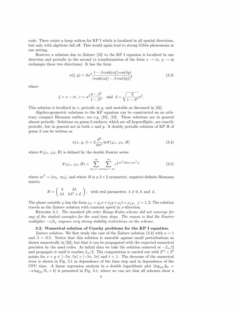
Fig. 3.1. Normalized L2 norm of the numerical error in the solution to the KP I equation withinitial data given by the Zaitsev solution for several numerical methods, as a function of Nt (left)and as a function of CPU time (right).

fourth order behavior: we find a = 4.32 for the Integrating Factor method, a = 4.38for Driscoll’s IMEX method, a = 3.93 for Krogstad’s ETD scheme, a = 4 for theCox-Matthews scheme, and a = 3.98 for the Hochbruck-Ostermann scheme. In thiscontext Driscoll’s IMEX method performs best, followed by the ETD schemes thathave almost identical performance (though the Hochbruck-Ostermann method usesmore internal time steps and thus more CPU time in Fig. 3.1). It can also be seenthat the various schemes do not show the phenomenon of order reduction as discussedin [24], which implies that the Zaitsev solution tests the codes in a non-stiff regime ofthe KP I equation.

Small dispersion limit for KP I. To study KP solutions in the limit of smalldispersion (ε → 0), we consider Schwartzian initial data satisfying the constraint(3.2). As in [33] we consider data of the form

u0(x, y) = −∂xsech2(R) where R =√x2 + y2. (3.6)

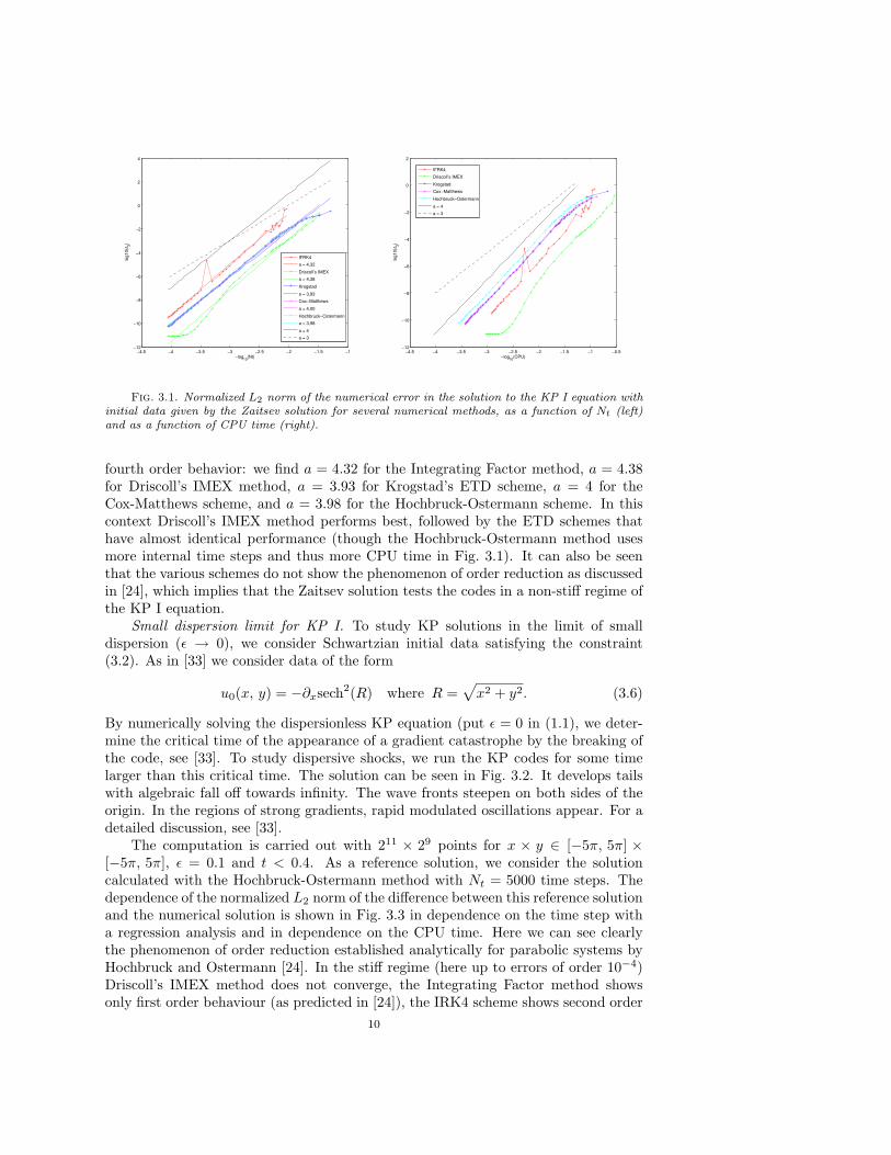
By numerically solving the dispersionless KP equation (put ε = 0 in (1.1), we deter-mine the critical time of the appearance of a gradient catastrophe by the breaking ofthe code, see [33]. To study dispersive shocks, we run the KP codes for some timelarger than this critical time. The solution can be seen in Fig. 3.2. It develops tailswith algebraic fall off towards infinity. The wave fronts steepen on both sides of theorigin. In the regions of strong gradients, rapid modulated oscillations appear. For adetailed discussion, see [33].

The computation is carried out with 211 × 29 points for x × y ∈ [−5π, 5π] ×[−5π, 5π], ε = 0.1 and t < 0.4. As a reference solution, we consider the solutioncalculated with the Hochbruck-Ostermann method with Nt = 5000 time steps. Thedependence of the normalized L2 norm of the difference between this reference solutionand the numerical solution is shown in Fig. 3.3 in dependence on the time step witha regression analysis and in dependence on the CPU time. Here we can see clearlythe phenomenon of order reduction established analytically for parabolic systems byHochbruck and Ostermann [24]. In the stiff regime (here up to errors of order 10−4)Driscoll’s IMEX method does not converge, the Integrating Factor method showsonly first order behaviour (as predicted in [24]), the IRK4 scheme shows second order

10

Fig. 3.2. Solution to the KP I equation for the initial data u0 = −∂xsech2(R) where R =px2 + y2 for several values of t.

−4 −3.5 −3 −2.5 −2 −1.5 −1−14

−12

−10

−8

−6

−4

−2

0

2

4

−log10

(Nt)

log10(Δ

2)

IFRK4

a = 1,87

Driscoll’s IMEX

a = 4,20

Krogstad

a = 3,75

Cox−Matthews

a = 3,90

Hochbruck−Ostermann

a = 3,96

Implicit RK4

a1 = 2,39

a2 = 4,03

a = 4

a = 3

−4.5 −4 −3.5 −3 −2.5 −2 −1.5 −1−14

−12

−10

−8

−6

−4

−2

0

2

4

−log10

(CPU)

log10(Δ

2)

IFRK4

Driscoll’s IMEX

Krogstad

Cox−Matthews

Hochbruck−Ostermann

Implicit RK4

a = 4

a = 3

Fig. 3.3. Normalized L2 norm of the numerical error for the solution shown in Fig. 3.2 forseveral numerical methods, as a function of Nt.

convergence, and ETD methods perform best. This implies that the Krogstad methodis the most economic for the stiff regime of the KP I equation, which gives the precisionone is typically interested in in this context. For higher precisions we find a = 1.87for the Integrating Factor method, a = 4.20 for Driscoll’s IMEX method, a = 4.03 forIRK4, a = 3.75 for Krogstad’s ETD scheme, a = 3.90 for the Cox-Matthews scheme,

11

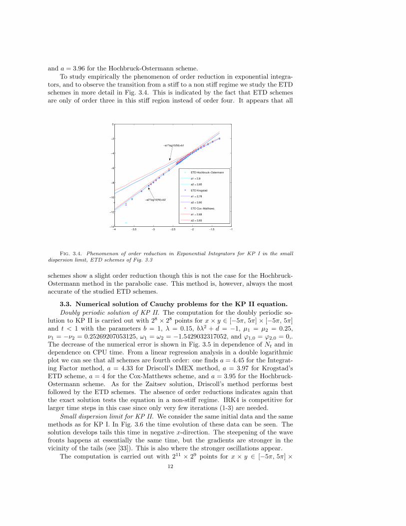
and a = 3.96 for the Hochbruck-Ostermann scheme.To study empirically the phenomenon of order reduction in exponential integra-

tors, and to observe the transition from a stiff to a non stiff regime we study the ETDschemes in more detail in Fig. 3.4. This is indicated by the fact that ETD schemesare only of order three in this stiff region instead of order four. It appears that all

−4 −3.5 −3 −2.5 −2 −1.5 −1−14

−12

−10

−8

−6

−4

−2

0

ETD Hochbruck−Ostermann

a1 = 2,8

a2 = 3,95

ETD Krogstad

a1 = 2,78

a2 = 3,90

ETD Cox−Matthews

a1 = 2,68

a2 = 3,93

−a1*log10(Nt)+b1

−a2*log10(Nt)+b2

Fig. 3.4. Phenomenon of order reduction in Exponential Integrators for KP I in the smalldispersion limit, ETD schemes of Fig. 3.3

schemes show a slight order reduction though this is not the case for the Hochbruck-Ostermann method in the parabolic case. This method is, however, always the mostaccurate of the studied ETD schemes.

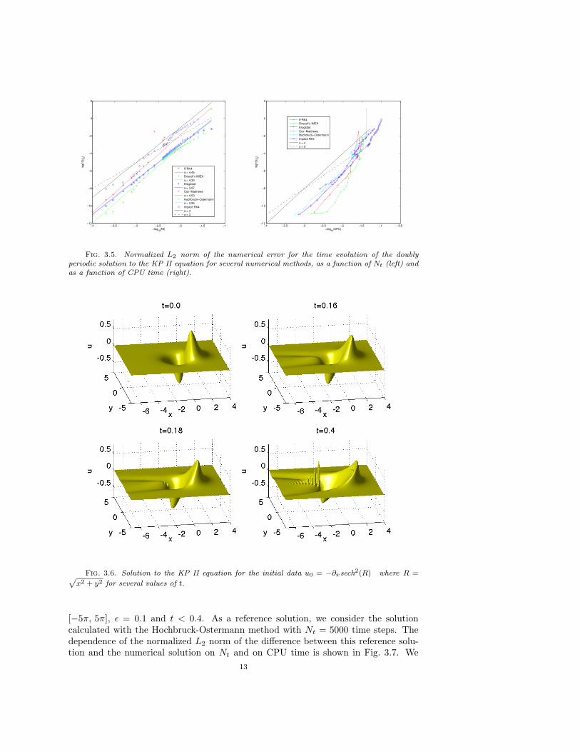
3.3. Numerical solution of Cauchy problems for the KP II equation.Doubly periodic solution of KP II. The computation for the doubly periodic so-

lution to KP II is carried out with 28 × 28 points for x × y ∈ [−5π, 5π] × [−5π, 5π]and t < 1 with the parameters b = 1, λ = 0.15, bλ2 + d = −1, µ1 = µ2 = 0.25,ν1 = −ν2 = 0.25269207053125, ω1 = ω2 = −1.5429032317052, and ϕ1,0 = ϕ2,0 = 0,.The decrease of the numerical error is shown in Fig. 3.5 in dependence of Nt and independence on CPU time. From a linear regression analysis in a double logarithmicplot we can see that all schemes are fourth order: one finds a = 4.45 for the Integrat-ing Factor method, a = 4.33 for Driscoll’s IMEX method, a = 3.97 for Krogstad’sETD scheme, a = 4 for the Cox-Matthews scheme, and a = 3.95 for the Hochbruck-Ostermann scheme. As for the Zaitsev solution, Driscoll’s method performs bestfollowed by the ETD schemes. The absence of order reductions indicates again thatthe exact solution tests the equation in a non-stiff regime. IRK4 is competitive forlarger time steps in this case since only very few iterations (1-3) are needed.

Small dispersion limit for KP II. We consider the same initial data and the samemethods as for KP I. In Fig. 3.6 the time evolution of these data can be seen. Thesolution develops tails this time in negative x-direction. The steepening of the wavefronts happens at essentially the same time, but the gradients are stronger in thevicinity of the tails (see [33]). This is also where the stronger oscillations appear.

The computation is carried out with 211 × 29 points for x × y ∈ [−5π, 5π] ×12

−4 −3.5 −3 −2.5 −2 −1.5 −1−12

−10

−8

−6

−4

−2

0

2

−log10

(Nt)

log10(Δ

2)

IFRK4

a = 4,45

Driscoll’s IMEX

a = 4,33

Krogstad

a = 3,97

Cox−Matthews

a = 4,00

Hochbruck−Ostermann

a = 3,95

Implicit RK4

a = 4

a = 3

−4 −3.5 −3 −2.5 −2 −1.5 −1 −0.5−12

−10

−8

−6

−4

−2

0

2

−log10

(CPU)

log10(Δ

2)

IFRK4

Driscoll’s IMEX

Krogstad

Cox−Matthews

Hochbruck−Ostermann

Implicit RK4

a = 4

a = 3

Fig. 3.5. Normalized L2 norm of the numerical error for the time evolution of the doublyperiodic solution to the KP II equation for several numerical methods, as a function of Nt (left) andas a function of CPU time (right).

Fig. 3.6. Solution to the KP II equation for the initial data u0 = −∂xsech2(R) where R =px2 + y2 for several values of t.

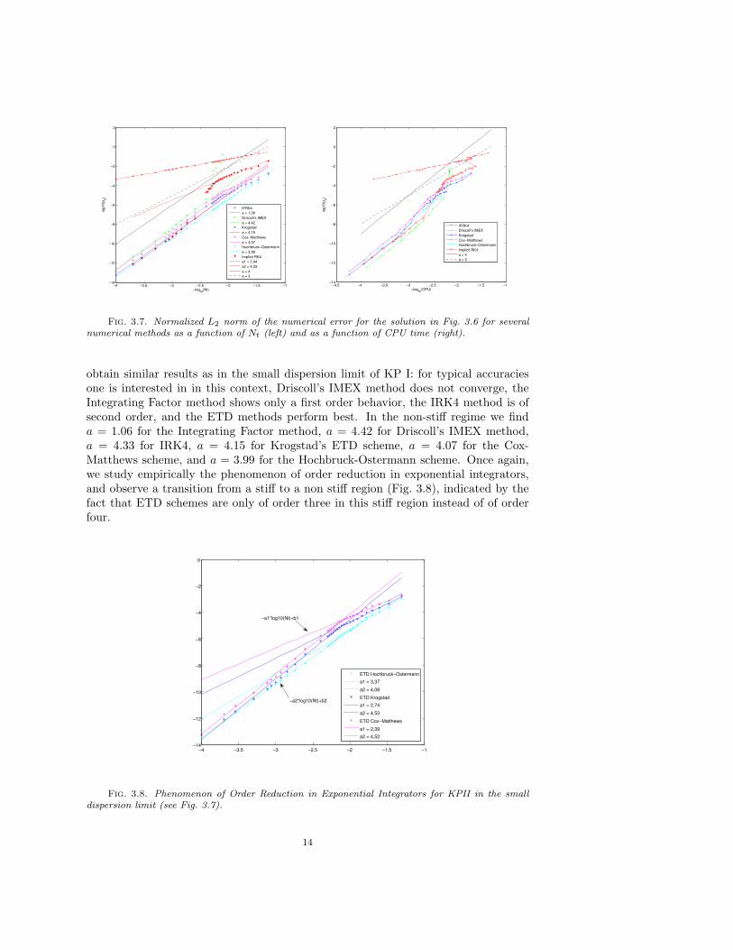
[−5π, 5π], ε = 0.1 and t < 0.4. As a reference solution, we consider the solutioncalculated with the Hochbruck-Ostermann method with Nt = 5000 time steps. Thedependence of the normalized L2 norm of the difference between this reference solu-tion and the numerical solution on Nt and on CPU time is shown in Fig. 3.7. We

13

−4 −3.5 −3 −2.5 −2 −1.5 −1−14

−12

−10

−8

−6

−4

−2

0

2

−log10

(Nt)

log10(Δ

2)

IFRK4

a = 1,06

Driscoll’s IMEX

a = 4,42

Krogstad

a = 4,15

Cox−Matthews

a = 4,07

Hochbruck−Ostermann

a = 3,99

Implicit RK4

a1 = 2,44

a2 = 4,33

a = 4

a = 3

−4.5 −4 −3.5 −3 −2.5 −2 −1.5 −1−14

−12

−10

−8

−6

−4

−2

0

2

−log10

(CPU)

log10(Δ

2)

IFRK4

Driscoll’s IMEX

Krogstad

Cox−Matthews

Hochbruck−Ostermann

Implicit RK4

a = 4

a = 3

Fig. 3.7. Normalized L2 norm of the numerical error for the solution in Fig. 3.6 for severalnumerical methods as a function of Nt (left) and as a function of CPU time (right).

obtain similar results as in the small dispersion limit of KP I: for typical accuraciesone is interested in in this context, Driscoll’s IMEX method does not converge, theIntegrating Factor method shows only a first order behavior, the IRK4 method is ofsecond order, and the ETD methods perform best. In the non-stiff regime we finda = 1.06 for the Integrating Factor method, a = 4.42 for Driscoll’s IMEX method,a = 4.33 for IRK4, a = 4.15 for Krogstad’s ETD scheme, a = 4.07 for the Cox-Matthews scheme, and a = 3.99 for the Hochbruck-Ostermann scheme. Once again,we study empirically the phenomenon of order reduction in exponential integrators,and observe a transition from a stiff to a non stiff region (Fig. 3.8), indicated by thefact that ETD schemes are only of order three in this stiff region instead of of orderfour.

−4 −3.5 −3 −2.5 −2 −1.5 −1−14

−12

−10

−8

−6

−4

−2

0

ETD Hochbruck−Ostermann

a1 = 3,37

a2 = 4,08

ETD Krogstad

a1 = 2,74

a2 = 4,53

ETD Cox−Matthews

a1 = 2,39

a2 = 4,52

−a1*log10(Nt)+b1

−a2*log10(Nt)+b2

Fig. 3.8. Phenomenon of Order Reduction in Exponential Integrators for KPII in the smalldispersion limit (see Fig. 3.7).

14

4. Davey-Stewartson equation. In this section we perform a similar studyas for KP of the efficiency of fourth methods in solving Cauchy problems for the DSequations. We first review some analytic facts about the focusing and defocusing DSII equations which are of importance in this context. We compare the performanceof the codes for a typical example in the small dispersion limit.

4.1. Analytic properties of the DS equations. For a review see for instancethe book by Sulem and Sulem [44]. The DS equation

iεut + ε2uxx − αε2uyy + 2ρ(

Φ + |u|2)u = 0,

Φxx + βΦyy + 2 |u|2xx = 0,(4.1)

where α, β and ρ take the values ±1 are classified [20] according to the ellipticity or hy-perbolicity of the operators in the first and second line. The case α = β is completelyintegrable and thus provides a 2 + 1-dimensional generalization of the integrable NLSequation in 1 + 1 dimensions. The integrable cases are elliptic-hyperbolic called DSI, and the hyperbolic-elliptic called DS II. For both there is a focusing (ρ = −1) anda defocusing (ρ = 1) version. We will study here only the DS II equations since theelliptic operator for Φ can be inverted by imposing simple boundary conditions. Fora hyperbolic operator acting on Φ boundary conditions for wave equations have to beused.

We will consider the equations again on T2 × R. Due to the ellipticity of theoperator in the equation for Φ, it can be inverted in Fourier space in standard mannerby imposing periodic boundary conditions on Φ as well. As before this case containsSchwartzian functions that are periodic for numerical purposes. Notice that solutionsto the DS equations for Schwartzian initial data stay in this space at least for finitetime in contrast to the KP case. Using Fourier transformations Φ can be eliminatedfrom the first equation by a transformation of the second equation in (1.2) and aninverse transformation. Writing the 2d-Fourier transform as

F [u] :=∫

R2u(x, y, t)e−ikxx−ikyydxdy,

we have

Φ = −2F−1

[k2x

k2x + k2

y

F[|u|2]],

which leads in (4.1) as for KP to a nonlocal equation with a singular Fourier multiplier.This implies that the DS equation requires an additional computational cost of 2 two-dimensional FFT per intermediate time step, thus doubling the cost with respect tothe standard 2d NLS equation. Notice that from a numerical point of view the sameapplies to the elliptic-elliptic DS equation that is not integrable. Our experimentsindicate that except for the additional FFT mentioned above, the numerical treatmentof the 2d and higher dimensional NLS is analogous to the DS II case studied here. Therestriction to this case is entirely due to the fact that one can hope for an asymptoticdescription of the small dispersion limit in the integrable case. Thus we study initialdata of the form u0(x, y) = a(x, y) exp(ib(x, y)/ε) with a, b ∈ R, i.e., the semi-classicallimit well known from the Schrodinger equation. Here we discuss only real initial datafor convenience.

15

It is known that DS solutions can have blowup. Results by Sung [45] establishglobal existence in time for initial data ψ0 ∈ Lp, 1 ≤ p < 2 with a Fourier transformF [ψ0] ∈ L1 ∩ L∞ subject to the smallness condition

||F [ψ0]||L1 ||F [ψ0]||L∞ <π3

2

(√5− 12

)2

(4.2)

in the focusing case. There is no such condition in the defocusing case. Notice thatcondition (4.2) has been established for the DS II equation with ε = 1. The coordinatechange x′ = x/ε, t′ = t/ε transforms the DS equation (1.2) to this standard form.This implies for the initial data u0 = exp(−x2−ηy2) we study for the small dispersionlimit of the focusing DS II system in this paper that condition (4.2) takes the form

1ε2η≤ 1

8

(√5− 12

)2

∼ 0.0477.

This condition is not satisfied for the values of ε and η we use here. Nonetheless wedo not observe any indication of blowup on the shown timescales. One of the reasonsis that the rescaling with ε above also rescales the critical time for blowup by a factor1/ε. In addition it is expected that the dispersionless equations will for generic initialdata have a gradient catastrophe at some time tc < ∞, and that the dispersion willregularize the solution for small times t > tc > 0. Since there are no analytical resultsfor these questions, careful numerical studies of the situation will be done.

The complete integrability of the DS II system implies again the existence ofexplicit solutions. Multi-soliton solutions will be as in the KP case localized in onespatial direction and infinitely extended in another. These solitons are not convenientto test codes based on Fourier methods since they will either have trivial angles withthe computational domain and thus depend only on one spatial coordinate, or havenon-trivial angles with this domain which will lead to Gibbs phenomena. The lumpsolution for DS II is localized in two spatial directions, but with an algebraic fall offtowards infinity which again leads to Gibbs phenomena. Since the study of the smalldispersion limit below indicates that the time steps have to be chosen sufficientlysmall for accuracy reasons that the equations are not stiff in contrast to KP (no orderreduction observed), we will not study any exact solutions here. First numericalstudies of exact solutions to the DS system were performed in [51]. In [5] blowup forDS was studied for the analytically known blowup solution by Ozawa [41].

4.2. Small dispersion limit for DS II in the defocusing case. We considerinitial data u0 of the form

u0(x, y) = e−R2, where R =

√x2 + y2, (4.3)

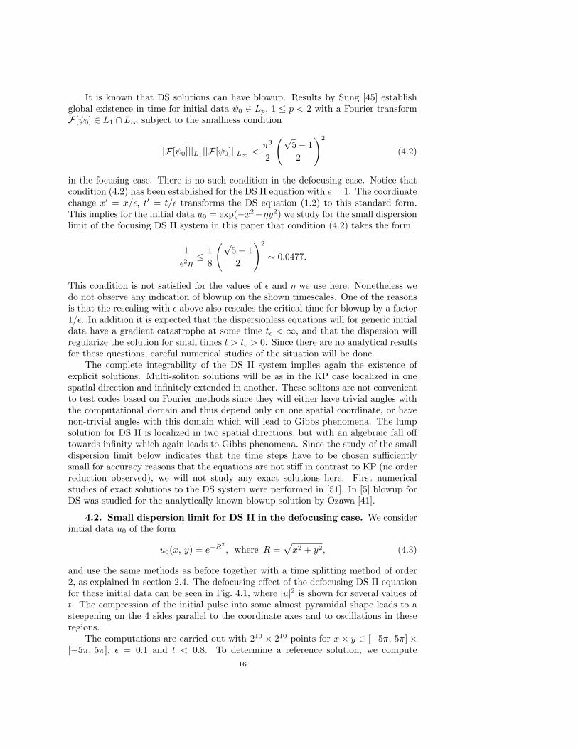
and use the same methods as before together with a time splitting method of order2, as explained in section 2.4. The defocusing effect of the defocusing DS II equationfor these initial data can be seen in Fig. 4.1, where |u|2 is shown for several values oft. The compression of the initial pulse into some almost pyramidal shape leads to asteepening on the 4 sides parallel to the coordinate axes and to oscillations in theseregions.

The computations are carried out with 210 × 210 points for x × y ∈ [−5π, 5π] ×[−5π, 5π], ε = 0.1 and t < 0.8. To determine a reference solution, we compute

16

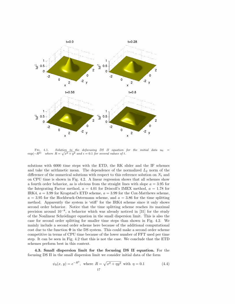
Fig. 4.1. Solution to the defocusing DS II equation for the initial data u0 =exp(−R2) where R =

px2 + y2 and ε = 0.1 for several values of t.

solutions with 6000 time steps with the ETD, the RK slider and the IF schemesand take the arithmetic mean. The dependence of the normalized L2 norm of thedifference of the numerical solutions with respect to this reference solution on Nt andon CPU time is shown in Fig. 4.2. A linear regression shows that all schemes showa fourth order behavior, as is obvious from the straight lines with slope a = 3.95 forthe Integrating Factor method, a = 4.01 for Driscoll’s IMEX method, a = 1.78 forIRK4, a = 3.99 for Krogstad’s ETD scheme, a = 3.99 for the Cox-Matthews scheme,a = 3.95 for the Hochbruck-Ostermann scheme, and a = 3.86 for the time splittingmethod. Apparently the system is ‘stiff’ for the IRK4 scheme since it only showssecond order behavior. Notice that the time splitting scheme reaches its maximalprecision around 10−8, a behavior which was already noticed in [31] for the studyof the Nonlinear Schrodinger equation in the small dispersion limit. This is also thecase for second order splitting for smaller time steps than shown in Fig. 4.2. Wemainly include a second order scheme here because of the additional computationalcost due to the function Φ in the DS system. This could make a second order schemecompetitive in terms of CPU time because of the lower number of FFT used per timestep. It can be seen in Fig. 4.2 that this is not the case. We conclude that the ETDschemes perform best in this context.

4.3. Small dispersion limit for the focusing DS II equation. For thefocusing DS II in the small dispersion limit we consider initial data of the form

ψ0(x, y) = e−R2, where R =

√x2 + ηy2 with η = 0.1 (4.4)

17

−4 −3.5 −3 −2.5 −2 −1.5 −1−18

−16

−14

−12

−10

−8

−6

−4

−2

0

−log10

(Nt)

log10(Δ

2) IFRK4

a = 3,95

Driscoll’s IMEX

a = 4,01

Krogstad

a = 3,99

Cox−Matthews

a = 3,99

Hochbruck−Ostermann

a = 3,95

Split Step 4

a = 3,86

Implicit RK4, a = 1,78

Split Step 2, a = 2

a = 4

a = 3

−4.5 −4 −3.5 −3 −2.5 −2 −1.5 −1 −0.5−14

−12

−10

−8

−6

−4

−2

0

−log10

(CPU)

log10(Δ

2)

IFRK4

Driscoll’s IMEX

Krogstad

Cox−Matthews

Hochbruck−Ostermann

Split Step 4

Split Step 2

Implicit Runge Kutta 4

a = 4

a = 3

a = 2

Fig. 4.2. Normalized L2 norm of the numerical error for several numerical methods for thesituation shown in Fig. 4.1 as a function of Nt (left) and of CPU time (right).

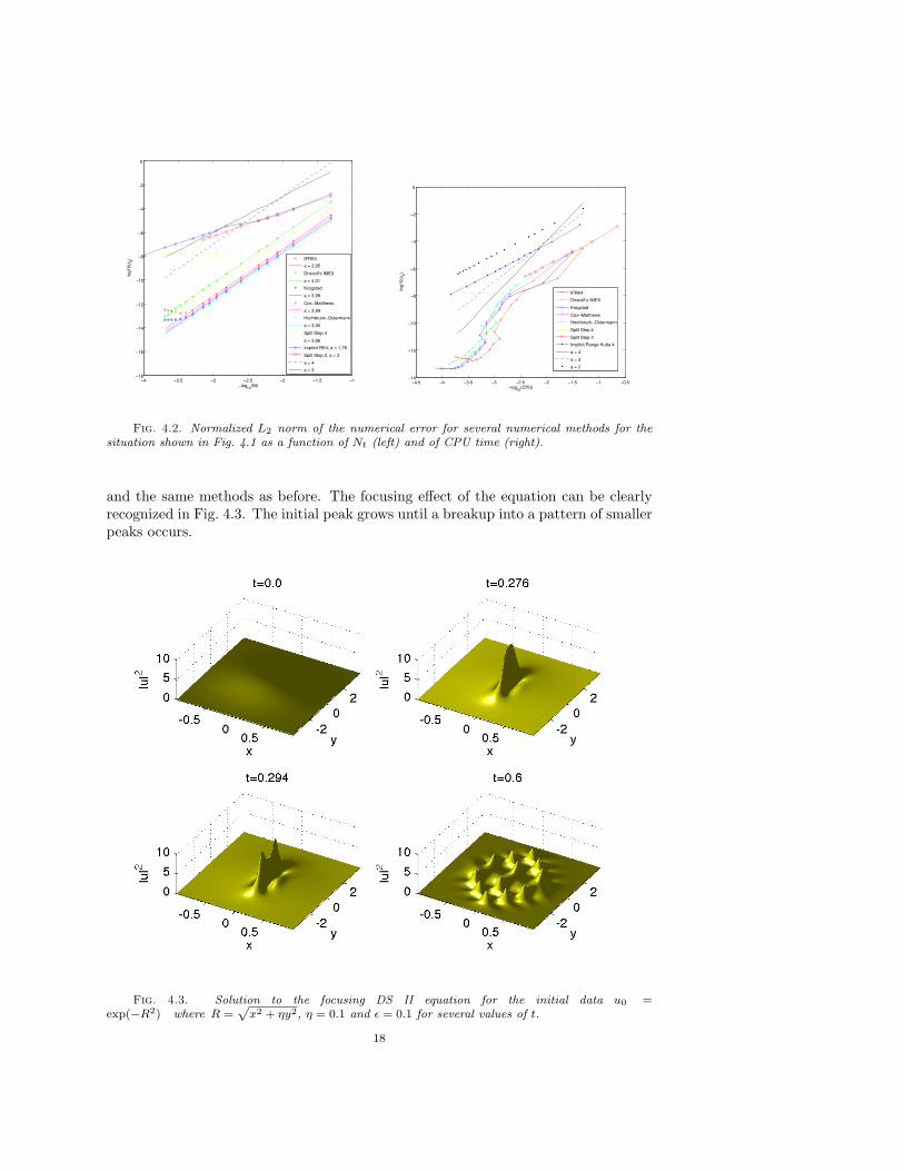
and the same methods as before. The focusing effect of the equation can be clearlyrecognized in Fig. 4.3. The initial peak grows until a breakup into a pattern of smallerpeaks occurs.

Fig. 4.3. Solution to the focusing DS II equation for the initial data u0 =exp(−R2) where R =

px2 + ηy2, η = 0.1 and ε = 0.1 for several values of t.

18

It is crucial to provide sufficient spatial resolution for the central peak. As forthe 1+1-dimensional focusing NLS discussed in [31], the modulational instability ofthe focusing DS II leads to numerical problems if there is no sufficient resolution forthe maximum. In [31] a resolution of 213 modes was necessary for initial data e−x

2

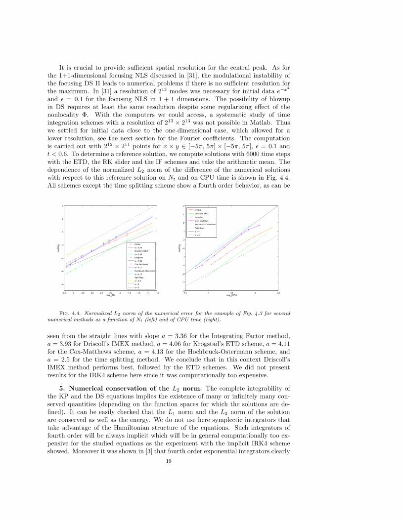
and ε = 0.1 for the focusing NLS in 1 + 1 dimensions. The possibility of blowupin DS requires at least the same resolution despite some regularizing effect of thenonlocality Φ. With the computers we could access, a systematic study of timeintegration schemes with a resolution of 213 × 213 was not possible in Matlab. Thuswe settled for initial data close to the one-dimensional case, which allowed for alower resolution, see the next section for the Fourier coefficients. The computationis carried out with 212 × 211 points for x × y ∈ [−5π, 5π] × [−5π, 5π], ε = 0.1 andt < 0.6. To determine a reference solution, we compute solutions with 6000 time stepswith the ETD, the RK slider and the IF schemes and take the arithmetic mean. Thedependence of the normalized L2 norm of the difference of the numerical solutionswith respect to this reference solution on Nt and on CPU time is shown in Fig. 4.4.All schemes except the time splitting scheme show a fourth order behavior, as can be

−3.2 −3 −2.8 −2.6 −2.4 −2.2 −2 −1.8 −1.6 −1.4 −1.2

−8

−6

−4

−2

0

2

4

−log10

(Nt)

log10(Δ

2)

IFRK4

a = 3,36

Driscoll’s IMEX

a = 3,93

Krogstad

a = 4,06

Cox−Matthews

a = 4,11

Hochbruck−Ostermann

a = 4,13

Split Step

a = 2,5

a = 4

a = 3

−4.5 −4 −3.5 −3 −2.5−8

−7

−6

−5

−4

−3

−2

−1

0

1

2

−log10

(CPU)

log10(Δ

2)

IFRK4

Driscoll’s IMEX

Krogstad

Cox−Matthews

Hochbruck−Ostermann

Split Step

a = 4

a = 3

Fig. 4.4. Normalized L2 norm of the numerical error for the example of Fig. 4.3 for severalnumerical methods as a function of Nt (left) and of CPU time (right).

seen from the straight lines with slope a = 3.36 for the Integrating Factor method,a = 3.93 for Driscoll’s IMEX method, a = 4.06 for Krogstad’s ETD scheme, a = 4.11for the Cox-Matthews scheme, a = 4.13 for the Hochbruck-Ostermann scheme, anda = 2.5 for the time splitting method. We conclude that in this context Driscoll’sIMEX method performs best, followed by the ETD schemes. We did not presentresults for the IRK4 scheme here since it was computationally too expensive.

5. Numerical conservation of the L2 norm. The complete integrability ofthe KP and the DS equations implies the existence of many or infinitely many con-served quantities (depending on the function spaces for which the solutions are de-fined). It can be easily checked that the L1 norm and the L2 norm of the solutionare conserved as well as the energy. We do not use here symplectic integrators thattake advantage of the Hamiltonian structure of the equations. Such integrators offourth order will be always implicit which will be in general computationally too ex-pensive for the studied equations as the experiment with the implicit IRK4 schemeshowed. Moreover it was shown in [3] that fourth order exponential integrators clearly

19

outperform second order symplectic integrators for the NLS equation.The fact that the conservation of L2 norm and energy is not implemented in

the code allows to use the ‘numerical conservation’ of these quantities during thecomputation or the lack thereof to test the quality of the code. We will study in thissection for the previous examples to which extent the numerical non-conservation isa quantitative indicator of numerical errors. Note that due to the non-locality of thestudied PDE (1.1) and (1.2), the energies both for KP,

E[u(t)] :=12

∫T2

(∂xu(t, x, y))2 − λ(∂−1

x ∂yu(t, x, y))2 − 2ε2u3(t, x, y))dxdy,

and for DS II,

E[u(t)] :=12

∫T2

((∂xu(t, x, y))2 − (∂yu(t, x, y))2

−ρε2

2(|u(t, x, y)|4 + Φ(t, x, y)2 + (∂−1

x ∂yΦ(t, x, y))2)dxdy),

contain anti-derivatives with respect to x. Since the latter are computed with Fouriermethods, i.e., via division by kx in Fourier space, this computation is in itself numeri-cally problematic and could indicate problems not present in the numerical solution ofthe Cauchy problem. Therefore we trace here only the L2 norm

∫T2 |u(t, x, y)|2dxdy,

where these problems do not appear.Notice that numerical conservation of the L2 norm can be only taken as an indi-

cation of the quality of the numerics if there is sufficient spatial resolution. Thereforewe will always present the Fourier coefficients for the final time step for the consideredexamples. We will discuss below the results for the small dispersion limit.

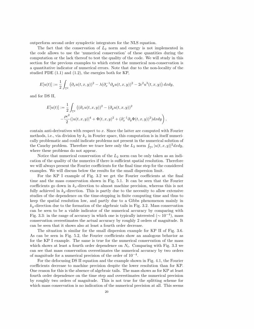
For the KP I example of Fig. 3.2 we get the Fourier coefficients at the finaltime and the mass conservation shown in Fig. 5.1. It can be seen that the Fouriercoefficients go down in kx-direction to almost machine precision, whereas this is notfully achieved in ky-direction. This is partly due to the necessity to allow extensivestudies of the dependence on the time-stepping in finite computing time and thus tokeep the spatial resolution low, and partly due to a Gibbs phenomenon mainly inky-direction due to the formation of the algebraic tails in Fig. 3.2. Mass conservationcan be seen to be a viable indicator of the numerical accuracy by comparing withFig. 3.3: in the range of accuracy in which one is typically interested (∼ 10−4), massconservation overestimates the actual accuracy by roughly 2 orders of magnitude. Itcan be seen that it shows also at least a fourth order decrease.

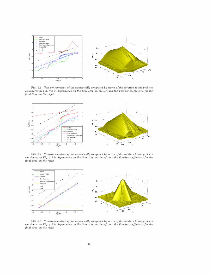
The situation is similar for the small dispersion example for KP II of Fig. 3.6.As can be seen in Fig. 5.2, the Fourier coefficients show an analogous behavior asfor the KP I example. The same is true for the numerical conservation of the masswhich shows at least a fourth order dependence on Nt. Comparing with Fig. 3.3 wecan see that mass conservation overestimates the numerical accuracy by two ordersof magnitude for a numerical precision of the order of 10−4.

For the defocusing DS II equation and the example shown in Fig. 4.1, the Fouriercoefficients decrease to machine precision despite the lower resolution than for KP.One reason for this is the absence of algebraic tails. The mass shows as for KP at leastfourth order dependence on the time step and overestimates the numerical precisionby roughly two orders of magnitude. This is not true for the splitting scheme forwhich mass conservation is no indication of the numerical precision at all. This seems

20

−4 −3.5 −3 −2.5 −2 −1.5 −1−20

−15

−10

−5

0

5

10

−log10

(Nt)

log

10

(te

st)

IFRK4

Driscoll’s IMEX

Krogstad

Cox−Matthews

Hochbruck−Ostermann

Implicit RK4

a = 5

a = 4

Fig. 5.1. Non-conservation of the numerically computed L2 norm of the solution to the problemconsidered in Fig. 3.3 in dependence on the time step on the left and the Fourier coefficients for thefinal time on the right.

−4 −3.5 −3 −2.5 −2 −1.5 −1−16

−14

−12

−10

−8

−6

−4

−2

0

2

−log10

(Nt)

log

10

(te

st)

IFRK4

Driscoll’s IMEX

Krogstad

Cox−Matthews

Hochbruck−Ostermann

Implicit RK4

a = 5

a = 4

Fig. 5.2. Non-conservation of the numerically computed L2 norm of the solution to the problemconsidered in Fig. 3.7 in dependence on the time step on the left and the Fourier coefficients for thefinal time on the right.

−4 −3.5 −3 −2.5 −2 −1.5 −1−16

−14

−12

−10

−8

−6

−4

−2

0

−log10

(Nt)

log

10

(te

st)

IFRK4

Driscoll’s IMEX

Krogstad

Cox−Matthews

Hochbruck−Ostermann

Split Step

a = 5

a = 4

Fig. 5.3. Non-conservation of the numerically computed L2 norm of the solution to the problemconsidered in Fig. 4.2 in dependence on the time step on the left and the Fourier coefficients for thefinal time on the right.

21

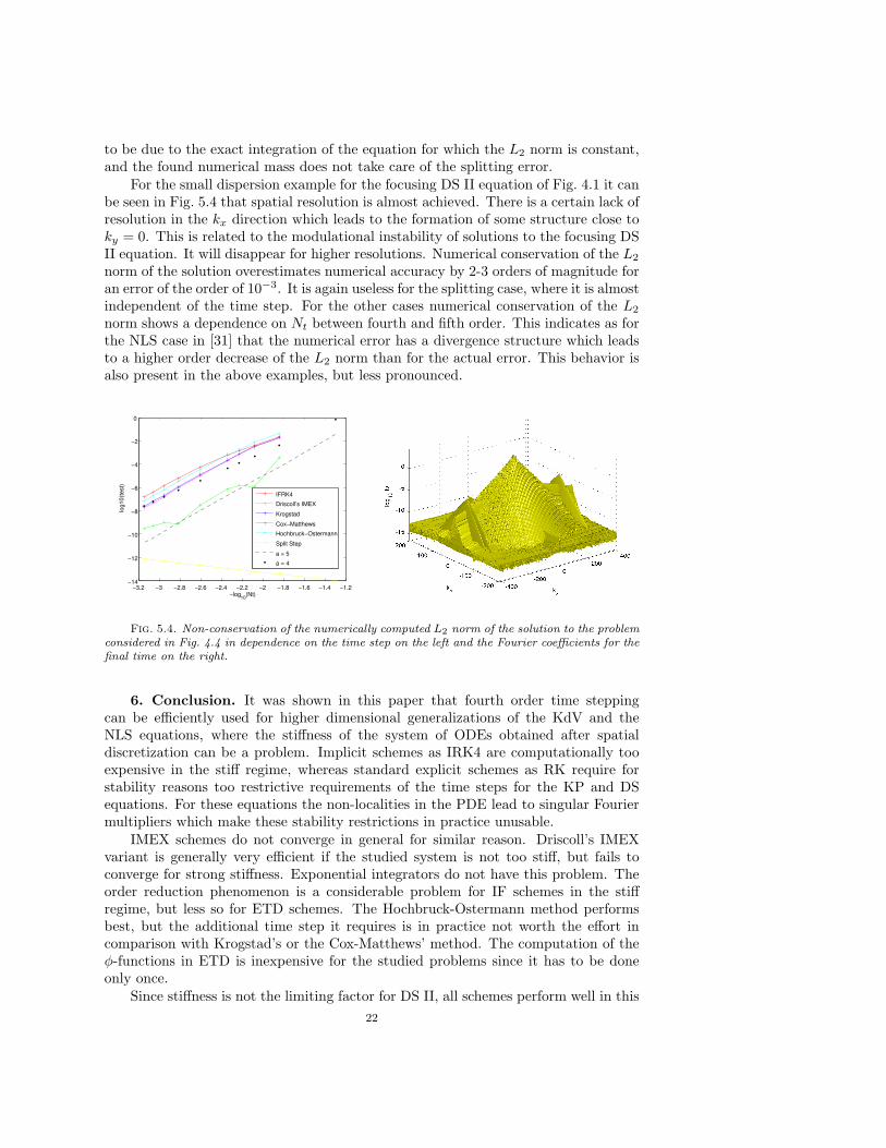
to be due to the exact integration of the equation for which the L2 norm is constant,and the found numerical mass does not take care of the splitting error.

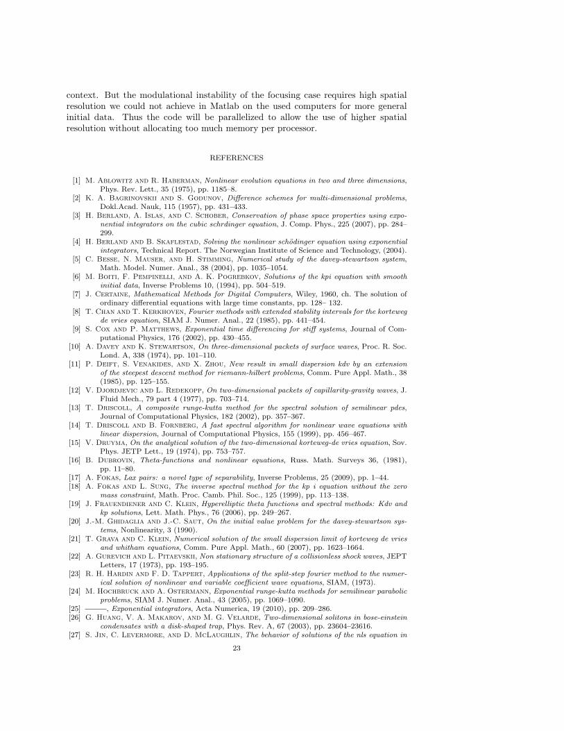
For the small dispersion example for the focusing DS II equation of Fig. 4.1 it canbe seen in Fig. 5.4 that spatial resolution is almost achieved. There is a certain lack ofresolution in the kx direction which leads to the formation of some structure close toky = 0. This is related to the modulational instability of solutions to the focusing DSII equation. It will disappear for higher resolutions. Numerical conservation of the L2

norm of the solution overestimates numerical accuracy by 2-3 orders of magnitude foran error of the order of 10−3. It is again useless for the splitting case, where it is almostindependent of the time step. For the other cases numerical conservation of the L2

norm shows a dependence on Nt between fourth and fifth order. This indicates as forthe NLS case in [31] that the numerical error has a divergence structure which leadsto a higher order decrease of the L2 norm than for the actual error. This behavior isalso present in the above examples, but less pronounced.

−3.2 −3 −2.8 −2.6 −2.4 −2.2 −2 −1.8 −1.6 −1.4 −1.2−14

−12

−10

−8

−6

−4

−2

0

−log10

(Nt)

log

10

(te

st)

IFRK4

Driscoll’s IMEX

Krogstad

Cox−Matthews

Hochbruck−Ostermann

Split Step

a = 5

a = 4

Fig. 5.4. Non-conservation of the numerically computed L2 norm of the solution to the problemconsidered in Fig. 4.4 in dependence on the time step on the left and the Fourier coefficients for thefinal time on the right.

6. Conclusion. It was shown in this paper that fourth order time steppingcan be efficiently used for higher dimensional generalizations of the KdV and theNLS equations, where the stiffness of the system of ODEs obtained after spatialdiscretization can be a problem. Implicit schemes as IRK4 are computationally tooexpensive in the stiff regime, whereas standard explicit schemes as RK require forstability reasons too restrictive requirements of the time steps for the KP and DSequations. For these equations the non-localities in the PDE lead to singular Fouriermultipliers which make these stability restrictions in practice unusable.

IMEX schemes do not converge in general for similar reason. Driscoll’s IMEXvariant is generally very efficient if the studied system is not too stiff, but fails toconverge for strong stiffness. Exponential integrators do not have this problem. Theorder reduction phenomenon is a considerable problem for IF schemes in the stiffregime, but less so for ETD schemes. The Hochbruck-Ostermann method performsbest, but the additional time step it requires is in practice not worth the effort incomparison with Krogstad’s or the Cox-Matthews’ method. The computation of theφ-functions in ETD is inexpensive for the studied problems since it has to be doneonly once.

Since stiffness is not the limiting factor for DS II, all schemes perform well in this22

context. But the modulational instability of the focusing case requires high spatialresolution we could not achieve in Matlab on the used computers for more generalinitial data. Thus the code will be parallelized to allow the use of higher spatialresolution without allocating too much memory per processor.

REFERENCES

[1] M. Ablowitz and R. Haberman, Nonlinear evolution equations in two and three dimensions,Phys. Rev. Lett., 35 (1975), pp. 1185–8.

[2] K. A. Bagrinovskii and S. Godunov, Difference schemes for multi-dimensional problems,Dokl.Acad. Nauk, 115 (1957), pp. 431–433.

[3] H. Berland, A. Islas, and C. Schober, Conservation of phase space properties using expo-nential integrators on the cubic schrdinger equation, J. Comp. Phys., 225 (2007), pp. 284–299.

[4] H. Berland and B. Skaflestad, Solving the nonlinear schodinger equation using exponentialintegrators, Technical Report. The Norwegian Institute of Science and Technology, (2004).

[5] C. Besse, N. Mauser, and H. Stimming, Numerical study of the davey-stewartson system,Math. Model. Numer. Anal., 38 (2004), pp. 1035–1054.

[6] M. Boiti, F. Pempinelli, and A. K. Pogrebkov, Solutions of the kpi equation with smoothinitial data, Inverse Problems 10, (1994), pp. 504–519.

[7] J. Certaine, Mathematical Methods for Digital Computers, Wiley, 1960, ch. The solution ofordinary differential equations with large time constants, pp. 128– 132.

[8] T. Chan and T. Kerkhoven, Fourier methods with extended stability intervals for the kortewegde vries equation, SIAM J. Numer. Anal., 22 (1985), pp. 441–454.

[9] S. Cox and P. Matthews, Exponential time differencing for stiff systems, Journal of Com-putational Physics, 176 (2002), pp. 430–455.

[10] A. Davey and K. Stewartson, On three-dimensional packets of surface waves, Proc. R. Soc.Lond. A, 338 (1974), pp. 101–110.

[11] P. Deift, S. Venakides, and X. Zhou, New result in small dispersion kdv by an extensionof the steepest descent method for riemann-hilbert problems, Comm. Pure Appl. Math., 38(1985), pp. 125–155.

[12] V. Djordjevic and L. Redekopp, On two-dimensional packets of capillarity-gravity waves, J.Fluid Mech., 79 part 4 (1977), pp. 703–714.

[13] T. Driscoll, A composite runge-kutta method for the spectral solution of semilinear pdes,Journal of Computational Physics, 182 (2002), pp. 357–367.

[14] T. Driscoll and B. Fornberg, A fast spectral algorithm for nonlinear wave equations withlinear dispersion, Journal of Computational Physics, 155 (1999), pp. 456–467.

[15] V. Druyma, On the analytical solution of the two-dimensional korteweg-de vries equation, Sov.Phys. JETP Lett., 19 (1974), pp. 753–757.

[16] B. Dubrovin, Theta-functions and nonlinear equations, Russ. Math. Surveys 36, (1981),pp. 11–80.

[17] A. Fokas, Lax pairs: a novel type of separability, Inverse Problems, 25 (2009), pp. 1–44.[18] A. Fokas and L. Sung, The inverse spectral method for the kp i equation without the zero

mass constraint, Math. Proc. Camb. Phil. Soc., 125 (1999), pp. 113–138.[19] J. Frauendiener and C. Klein, Hyperelliptic theta functions and spectral methods: Kdv and

kp solutions, Lett. Math. Phys., 76 (2006), pp. 249–267.[20] J.-M. Ghidaglia and J.-C. Saut, On the initial value problem for the davey-stewartson sys-

tems, Nonlinearity, 3 (1990).[21] T. Grava and C. Klein, Numerical solution of the small dispersion limit of korteweg de vries

and whitham equations, Comm. Pure Appl. Math., 60 (2007), pp. 1623–1664.[22] A. Gurevich and L. Pitaevskii, Non stationary structure of a collisionless shock waves, JEPT

Letters, 17 (1973), pp. 193–195.[23] R. H. Hardin and F. D. Tappert, Applications of the split-step fourier method to the numer-

ical solution of nonlinear and variable coefficient wave equations, SIAM, (1973).[24] M. Hochbruck and A. Ostermann, Exponential runge-kutta methods for semilinear parabolic

problems, SIAM J. Numer. Anal., 43 (2005), pp. 1069–1090.[25] , Exponential integrators, Acta Numerica, 19 (2010), pp. 209–286.[26] G. Huang, V. A. Makarov, and M. G. Velarde, Two-dimensional solitons in bose-einstein

condensates with a disk-shaped trap, Phys. Rev. A, 67 (2003), pp. 23604–23616.[27] S. Jin, C. Levermore, and D. McLaughlin, The behavior of solutions of the nls equation in

23

the semiclassical limit, in Singular Limits of Dispersive Waves, 1994.[28] B. B. Kadomtsev and V. I. Petviashvili, On the stability of solitary waves in weakly dis-

persing media, Sov. Phys. Dokl., 15 (1970), pp. 539–541.[29] S. Kamvissis, K.-R. McLaughlin, and P. Miller, Semiclassical Soliton Ensembles for the

Focusing Nonlinear Schrodinger Equation, Princeton University Press, 2003.[30] A.-K. Kassam and L. Trefethen, Fourth-order time-stepping for stiff pdes, SIAM J. Sci.

Comput, 26 (2005), pp. 1214–1233.[31] C. Klein, Fourth order time-stepping for low dispersion korteweg-de vries and nonlinear

schrodinger equation, Electronic Transactions on Numerical Analysis., 39 (2008), pp. 116–135.

[32] C. Klein and J.-C. Saut, Numerical study of blow up and stability of solutions of generalizedkadomtsev-petviashvili equations, preprint, arXiv:1010.5510, (2010).

[33] C. Klein, C. Sparber, and P. Markowich, Numerical study of oscillatory regimes in thekadomtsev-petviashvili equation, J. Nonl. Sci., 17 (2007), pp. 429–470.

[34] S. Krogstad, Generalized integrating factor methods for stiff pdes, Journal of ComputationalPhysics, 203 (2005), pp. 72–88.

[35] J. Lawson, Generalized runge-kutta processes for stable systems with large lipschitz constants,SIAM J. Numer. Anal., 4 (1967).

[36] P. Lax and C. Levermore, The small dispersion limit of the korteweg de vries equation i, ii,iii, Comm. Pure Appl. Math., 36 (1983), pp. 253–290, 571–593, 809–830.

[37] B. Minchev and W. Wright, A review of exponential integrators for first order semi-linearproblems, Technical Report 2, The Norwegian University of Science and Technology, (2005).

[38] L. Molinet, J. C. Saut, and N. Tzvetkov, Remarks on the mass constraint for kp typeequations, SIAM J. Math. Anal., 39 (2007), pp. 627–641.

[39] K. Nishinari, K. Abe, , and J. Satsuma, A new type of soliton behaviour in a two dimensionalplasma system, J. Phys. Soc. Jpn., 62 (1993), pp. 2021–2029.

[40] , Multidimensional behavior of an electrostaic ion wave in a magnetized plasma, Phys.Plasmas, 1 (1994), pp. 2559–2565.

[41] T. Ozawa, Exact blow-up solutions to the cauchy problem for the davey-stewartson systems,Proc. R. Soc. Lond. A, 436 (1992), pp. 345–349.

[42] T. Schmelzer, The fast evaluation of matrix functions for exponential integrators, PhD thesis,Oxford University, 2007.

[43] G. Strang, On the construction and comparison of difference shemes, SIAM J. Numer. Anal.,5 (1968), pp. 506–517.

[44] C. Sulem and P. Sulem, The nonlinear Schrodinger equation, Springer, 1999.[45] L.-Y. Sung, Long-time decay of the solutions of the davey-stewartson ii equations, J. Nonlinear

Sci, 5 (1995), pp. 433–452.[46] F. Tappert, Numerical solutions of the korteweg-de vries equation and its generalizations by

the split-step fourier method, Lectures in Applied Mathematics, 15 (1974), pp. 215–216.[47] A. Tovbis, S. Venakides, and X. Zhou, On semiclassical (zero dispersion limit) solutions of

the focusing nonlinear schrodinger equation, Communications on pure and applied math-ematics, 57 (2004), pp. 877–985.

[48] H. Trotter, On the product of semi-groups of operators, Proceedings of the American Math-ematical Society, 10 (1959), pp. 545–551.

[49] S. Turitsyn and G. Falkovitch, Stability of magneto-elastic solitons and self-focusing ofsound in antiferromagnets, Soviet Phys. JETP, 62 (1985), pp. 146–152.

[50] S. Venakides, The zero dispersion limit of the korteweg de vries equation for initial potentialwith nontrivial reflection coefficient, Comm. Pure Appl. Math., 38 (1985), pp. 125–155.

[51] P. White and J. Weideman, Numerical simulation of solitons and dromions in the davey-stewartson system, Math. Comput. Simul., 37 (1994), pp. 469–479.

[52] H. Yoshida, Construction of higher order symplectic integrators, Physics Letters A, 150 (1990),pp. 262–268.

[53] A. Zaitsev, Formation of stationary waves by superposition of solitons, Sov. Phys. Dokl., 25(1983), pp. 720–722.

24