NASA Technical Memorandum 109112

/H --o 211

Fourth-Order 2N-Storage Runge-Kutta Schemes

Mark H. CarpenterLangley Research Center, Hampton, Virginia

Christopher A. Kennedy

University of CMifornia, San Diego, La JoHa, California

(NASA-TM-I09112) FOURTH-ORDER

2N-STORAGE RUNGE-KUTTA SCHEMES

(NASA. Langley Research Center)

26 p

N94-32950

Uncl a s

June 1994G3/02 0009987

National Aeronautics and

Space Administration

Langley Research Center

Hampton, Virginia 23681-0001

FOURTH-ORDER 2N-STORAGE RUNGE-KUTTA SCHEMES

Mark It. Carpenter _ Christopher A. Kennedy t

Abstract

A family of five-stage fourth-order Runge-Kutta schemes is derived; these schemes require only two

storage locations. A particular scheme is identified that has desirable efficiency characteristics for

hyperbolic and parabolic initial (boundary) value problems. This scheme is competitive with the

classical fourth-order method (high-storage) and is considerably more efficient and accurate than

existing third-order low-storage schemes.

Section 1: Introduction

Many problems of mathematical physics result in the numerical approximation of systems of

coupled ordinary differential equations (ODE's). The technique for integrating the equations depends

on, among other things, the desired accuracy, efficiency, robustness, and simplicity. For the ODE's

that result from tile direct simulation of the equations of fluid dynamics, the overriding consideration

is often the availability of fast memory. A numerical integration technique that minimizes memory

storage is essential and can be formulated with a Runge-Kutta (RK) methodology.

Williamson [1] showed that all second-order and some third-order RK schemes can be cast in a

2N-storage format, where N is the dimension of tile system of ODE's. He also showed that (except

for certain exceptional cases that involve specific forms of the function to be integrated) tile four-

stage fourth-order RK schemes cannot be put into 2N-storage format. Fyfe [2] showed that all

four-stage fourth-order RK schemes can be implemented in 3N-storage locations. In spite of the

reduced accuracy, for many apl)lications the methods of choice are tile 2N-storage third-order RK

scllelIle$.

Although the principal motivation of this work is to derive schemes of 2N storage, both the

accuracy and elliciency also determine the practical utility of any scheme. For example, a fourth-

order 2N-storage scheme with a vanishingly small stability envelope is of little practical value. Tile

*Aerospace Engineer, Theoretical Flow Physics Branch, NASA Langley Research Center, Itampton, VA 23681.

tApplied Mecha.ics and Engineering Sciences, University of California, San Diego, La Jolla, CA 92093.

efficiency of an RK scheme is determined by the absolute size of the stability domain relative to the

number of stages needed tO implement the scheme. Typically, RK schemes that utilize the mininmm

number of stages necessary to achieve a given order of accuracy are used because they minimize the

absolute workload for a given order of accuracy. Verner [3], however, demonstrated that the 13-stage

eighth-order scheme is more effÉcient than the 12-stage eighth-order scheme. Similarly, Sharp et al.

[4] showed that the efficiency of many existing fifth-, sixth-, and seventh-order RK schemes can be

increased by including additional stages while retaining the same order of accuracy. The additional

stages are used to optimize the absolute stability domain and increase the relative efficiency of each

stage.

A five-stage fourth-order RK scheme that satisfies the 2N-storage constraint is sought. The scheme

should have the largest absolute linear stability envelope and the lowest truncation error possible.

In section 2, we describe the conventional and the 2N-storage RK nomenclature. In section 3, we

derive the complete set of three-stage third-order (3,3) RK schemes that can be cast in 2N-storage

format. We then introduce a new set of four-stage third-order (4,3) RK schemes that are 2N-storage

schemes. In section 4, we derive the new five-stage fourth-order (5,4) RK schemes that require 2N

storage. In section 5, we compare all schemes for efficiency, accuracy, and simplicity and then draw

conclusions in regard to the utility of the new schemes.

Section 2: Runge-Kutta Nomenclature

We are concerned with the numerical solution of the initial value problem

dU

d'--[ = F[t,U(t)]; U(to) --, Uo

Assume that the discrete approximation is made with an M-stage explicit RK scheme. The imple-

mentation over a time step h is accomplished by

kl = F(to, U °)

ki = F to + cih, V 0 @ h E ai,jkj

j=l /M

v = v ° + bjkjj=l

i = 2,...,M

where U ° = U(to) and U _ = U(to + h) and the fixed scalars ai,j, bj, ci are the coefficients of the RK

formula.

Butcher [5] developed a succinct nomenclature for writing all RK schemes in terms of the fixed

scalar coefficients ai,j, bj, ci. The general, M-stage, explicit ILK scheme can be expressed as

c1

g2,1

CM aM,1 aM,M_ 1

bl bM

The entries in the first column (ci, i = 1, M) are the intermediate time levels. The coefficients ai,j

are the intermediate weights of each RK stage i. By definition, ci = _jM 1 ai,j and cl = 0 for the

explicit self-starting case. The last row (bj, j = 1, M) are the weights of the final stage.

To devise low-storage RK schemes, Williamson and Fyfe exploit the technique of leaving useful

information in the storage register. Each successive stage is written onto the same register without

zeroing the previous value. Thus, the M-stage algorithm becomes

dUj = AjdUj_I +

uj = vj_l +So that the algorithm is self-starting, A1 = 0.

results in a 2N-storage algorithm.

hF(U_)

BjdUj j= 1, M

Only the dU and U vectors must be stored, which

Williamson [1] first presented the relationship between the general RK scheme and the 2N-storage

scheme. Specifically, the following equations provide the relationship between the 2N-storage vari-

ables Aj and Bj and the conventional RK variables al,j, bj, and ci:

Bj = aj+l,j (j # M)BM _-- bM

Aj = (bj__ - Bj_l)/bj (j _ 1,bj # 0) (1)

Aj -" (aj+lj-1-cj)/Bj (j # 1, bj =0)

The precise values of Aj and Bj that are required to yield a higher order scheme remain to be

determined. Third-order RK schemes are the lowest order schemes for which the determination of

2N-storage is nontrivial. We begin by demonstrating the procedure for finding high-order 2N storage

ILK schemes for the third-order case.

Section 3: Third-Order Runge-Kutta Methods

For a third-order Runge-Kutta scheme, at least three stages are required. The general Butcher

array diagram for the three-stage explicit scheme is written as

C2 a2,1

c3 ] a3,1 a3,2

I bi b2 b3

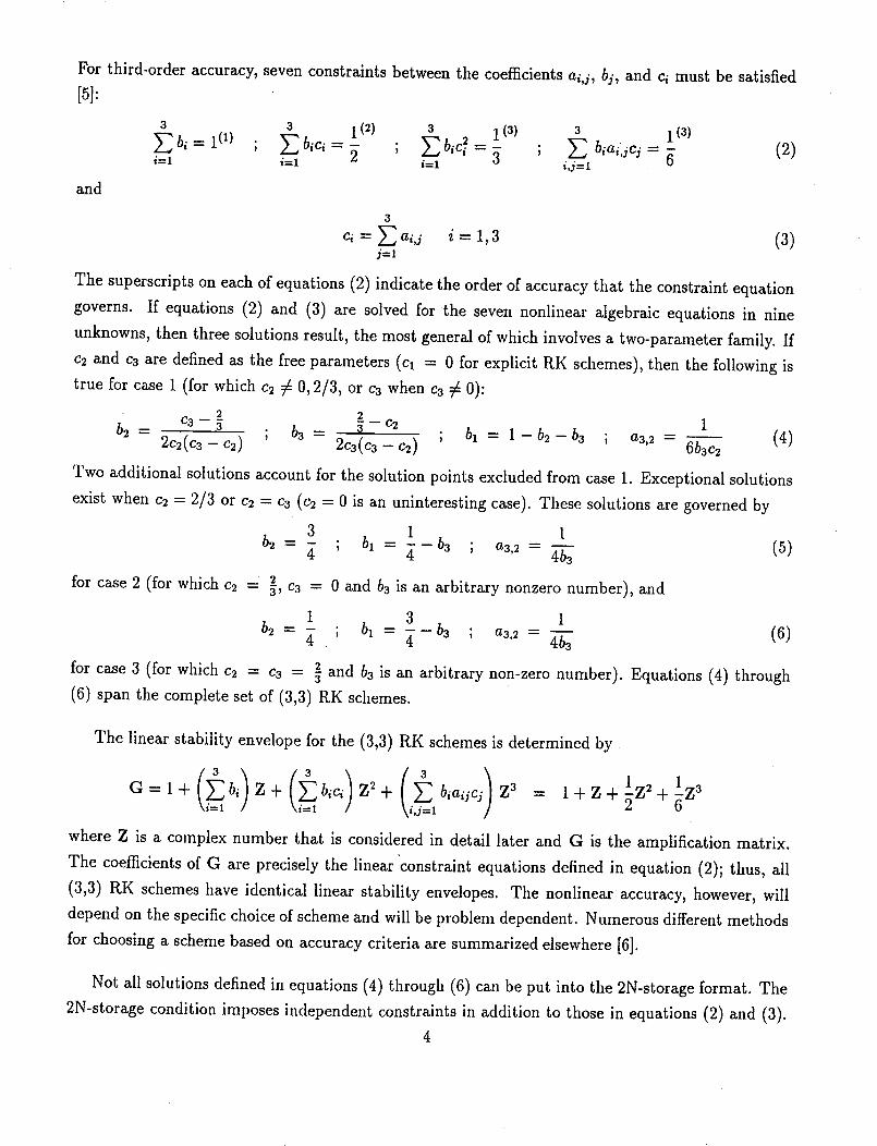
For third-order accuracy, seven constraints between the coefficients ai,j, bi, and c/must be satisfied

[5]:

3 3 1 (2) 3 1(3) 3 1 (3)b, = l (1) ; _bic,=- ; _ bic_ = - ; Y_ biai:jcj = (2)

i=1 _=1 2 i=l 3i,j=l

and

3

ci = _aij i= 1,3 (3)j=l

The superscripts on each of equations (2) indicate the order of accuracy that the constraint equation

governs. If equations (2) and (3) are solved for the seven nonlinear algebraic equations in nine

unknowns, then three solutions result, the most general of which involves a two-parameter family. If

c2 and c3 are defined as the free parameters (Cl = 0 for explicit RK schemes), then the following is

true for case 1 (for which c2 # 0,2/3, or c3 when c3 # 0):

2 2c3 - _ - - 1

b2 = 2c2(c3 -- C2) ; b3 -- 3 c22c3(c3-c2) ; bl= X-b2-b3 ; a3.2 = 6b3c 2 (4)

Two additional solutions account for the solution points excluded from case 1. Exceptional solutions

exist when c2 = 2/3 or c2 = c3 (c2 = 0 is an uninteresting case). These solutions are governed by

3 1 1

b2 = _ ; bl = _-b3 ; a3,2 = _3 (5)

for case 2 (for which c2 = 2, c3 = 0 and b3 is an arbitrary nonzero number), and

1 3 1

b2 = _- ; bl -- _--b3 ; a3,2 = 4b-_ (6)

for case 3 (for which c2 = c3 = 32-and b3 is an arbitrary non-zero number). Equations (4) through

(6) span the complete set of (3,3) RK schemes.

The linear stability envelope for the (3,3) RK schemes is determined by

G = 1 + bi Z + bici Z 2 q- biaijcj Z 3 = 1 2t- Z -)t- _Z 71" Z 3i,j=l

where Z is a complex number that is considered in detail later and G is the amplification matrix.

The coefficients of G are precisely the linearconstraint equations defined in equation (2); thus, all

(3,3) ILK schemes have identical linear stability envelopes. The nonlinear accuracy, however, will

depend on the specific choice of scheme and will be problem dependent. Numerous different methods

for choosing a scheme based on accuracy criteria are summarized elsewhere [6].

Not all solutions defined in equations (4) through (6) can be put into the 2N-storage format. The

2N-storage condition imposes independent constraints in addition to those in equations (2) and (3).

4

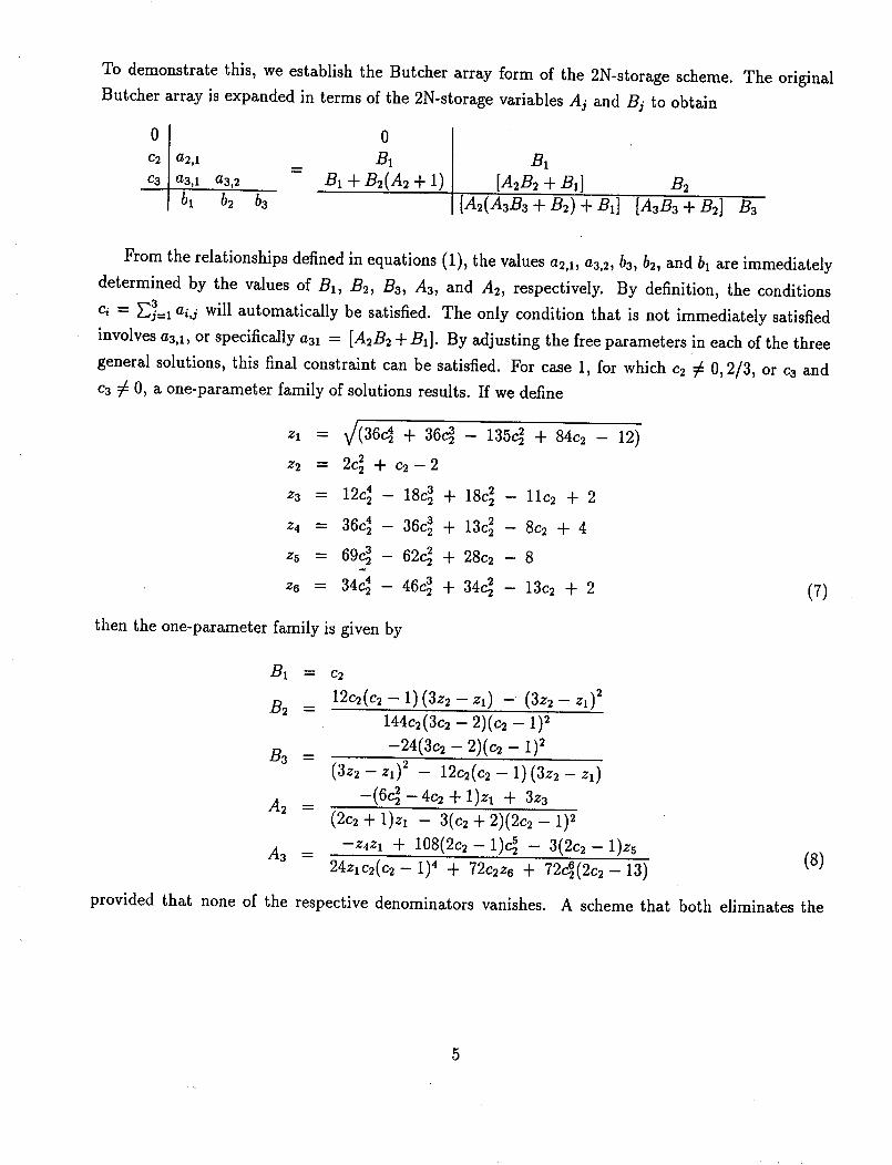
To demonstratethis, weestablishthe Butcher array form of the 2N-storage scheme. The original

Butcher array is expanded in terms of the 2N-storage variables Aj and Bj to obtain

oI 0C2 a2,1 B1

c3 a3a a3a = BI + B2(A2 + I)

bl b2 b3

B1

[A2B2 + B1] B2

[A2(AaB3 + B2) + B1] [A3B3 + B2] Ba

From the relationships defined in equations (1), the values a2,1, a3,2, b3, b2, and bl are immediately

determined by the values of B1, B2, B3, A3, and A2, respectively. By definition, the conditions

ci = _=1 ai.j will automatically be satisfied. The only condition that is not immediately satisfied

involves a3a, or specifically a31 = [A2B2 + B1]. By adjusting the free parameters in each of the three

general solutions, this final constraint can be satisfied. For case 1, for which c2 # 0, 2/3, or c3 and

c3 # 0, a one-parameter family of solutions results. If we define

zl = _/i36c24 + 36c23 - 135c_ + 84c2- 12)

z2 = 2c_ + c2-2

za = 12c_- 18c_ + 18c_- 11c2 + 2

z4 = 36c 4 - 36c 3 + 13c] - 8c2 + 4

zs = 69c23 - 62c_ + 28c2 - 8

zs = 34c_ - 46c23 + 34c] - 13c2 + 2 (7)

then the one-parameter family is given by

B1 --

B2 =

B3

A s =

A 3 =

provided that none of the respective denominators vanishes.

C2

12c2(c2 - 1)(3z2- Zl) - (3z2- Zl) 2

144c2(3c2- 2)(c2- 1) 2

-24(3c2- 2)(c2- 1) 2

(3z2- z,) 2 - 12c2(c2- 1) (3z2 - z,)

-(6c_ - 4c2 + 1)zx + 3z3

(2c2 + 1)Zl - 3(c2 + 2)(2c2 - 1) 2

-z4z, + 108(2c2- l)c_ - 3(2c_ - l)zs

24z_c2(c2-i) 4 + 72c2z6 + 72c_(2c2-13) (8)

A scheme that both eliminates the

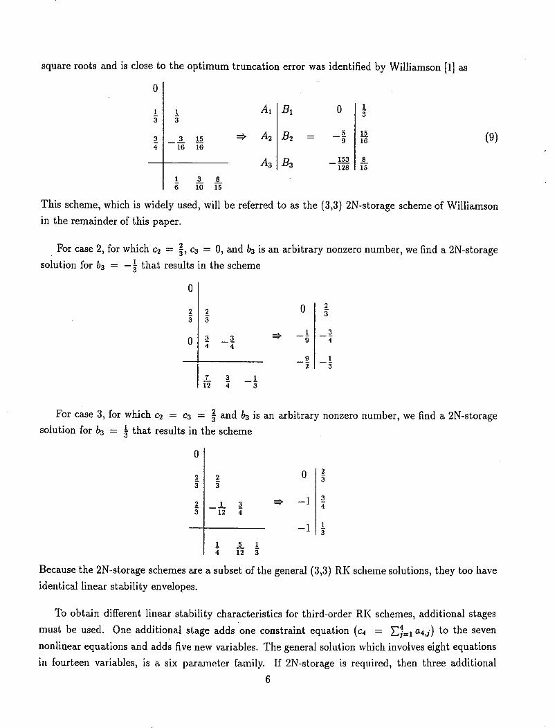
square roots and is close to the optimum truncation error was identified by Williamson [1] as

0

3 15 ==_

16 16

1 3 86 10 15

A1

A2

A3

B1

B2 =

B3

03

_: :s9 16

153 8

128 15

(9)

This scheme, which is widely used, will be referred to as the (3,3) 2N-storage scheme of Williamson

in the remainder of this paper.

For case 2, for which c2 = ], c3 = 0, and b3 is an arbitrary nonzero number, we find a 2N-storage

solution for b3 -- -:: that results in the scheme

0

23

0 3 3 =_4 4

r. 3_ _I12 4 3

0 23

1 3-: -7

9 1

2 3

2 and b3 is an arbitrary nonzero number, we find a 2N-storageFor case 3, for whichc2 = c3 = :

: that results in the schemesolution for b3 = :

0

112 4

3 =_

1 5 1

4 12 3

0 23

-1 3_4

-1 13

Because the 2N-storage schemes are a subset of the general (3,3) RK scheme solutions, they too have

identical linear stability envelopes.

To obtain different linear stability characteristics for third-order RK schemes, additional stages

must be used. One additional stage adds one constraint equation (c4 4= _]j=l a,j) to the seven

nonlinear equations and adds five new variables. The general solution which involves eight equations

in fourteen variables, is a six parameter family. If 2N-storage is required, then three additional

6

equations must be satisfied, which eliminates three of the six free parameters. The general four-stage

third-order (4,3) RK solution that involves 2N-storage can be expressed as a three-parameter family.

A two-parameter family may be generated by enforcing the linear, fourth-order constraint. None of

these general expressions are presented here because of their complexity.

If third-order accuracy is achieved" in four stages instead of three, then the required work per

time step is increased by one third. By en_0rcing the linear, fourth-order constraint, the increased

stability envelope of the (4,3) R.K schemes mpre than offsets this additional work. The (4,3) schemes

are more efficient per unit time, which is consistent with the work of Sharp et al. [4]. An extensive

study of the stability domains of the (4,3) R.K schemes shows that a nearly optimal scheme can be

obtained by setting

G----I+ (i__lbi) Z+ (_=lbici)Z2-t - (_i,j=lblaijcj)Z3-4 - (i,j,k=l_ biaijajkck)Z 4

= l+Z+ Z2+ Z3+=-:Z

Note that these schemes are third-order accurate for the nonlinear problem but fourth-order accurate

for the linear problem. Three third-order schemes that satisfy the 2N-storage constraint in four stages

and have a nearly optimal stability envelope are now presented. If we set c2 = c3, then

0

z_3

1

3

1

! 03

-15 3

12 4 =_

£ i 2 -i4 12 3

-1

N 1 5 13 12 4

(10)

If we set c3 = c4, then

0

14

11

12

II

14

11 1136 9

419 16 18

12 396 9 II

1 3 17 1

11 4 66 12

:=_

0 !4

5 II

II 9

II 18

6 II

182 1

II 12

19

36

3

or 4

0

19

36

51 27

76 19

3 19 n 2

13 27 1

57 76 6

=_243

243

38

_29

O 1936

205 27

19

2

9

I4

7

If we demand that the intermediate time levels cj be monitonically increasing, then

0

19

4

19

11 3

9 36 4

6 1 7 2

12 20 5

-I 2 5 s4 4

=:_

0 19

5 3

9 4

-1 2_5

33 5

25 4

or

3_ 39 9

5

9

8_9

S 5_. 15

18 6

5

4"1 1 3 390 6 5

-1

3 i 7 120 4 20 4

0 13

II 56

3

5

L4

For problems in which third-order temporal accuracy is sufficient, these new schemes should be

considered because of their larger stability envelope.

Section 4: Fourth-Order l:tunge-Kutta

Twelve nonlinear algebraic equations in fourteen variables determine the solution to the four-stage

fourth-order (4,4) RK schemes. Five general solutions exist: one that involves two free parameters

and four that involve one free parameter, covering the special roots excluded by the first. (See

Butcher for the general solutions [5].) Fyfe [2] demonstrated that all cases can be implemented in

the 3N-storage format. Williamson [1] demonstrated that they could not, in general, be implemented

in the 2N-storage format. The 2N-storage constraint adds three additional equations that cannot be

satisfied by any of the five general solutions.

By increasing the number of stages, additional degrees of freedom are generated that can be used

to satisfy all fourth-order and 2N-storage constraint equations. The five-stage fourth-order (5,4) RK

scheme may be expressed in Butcher and 2N-storage form as

el

C2

C3

C4

C5

a2,1

a3,1 a3,2

a4,1 a4,2 a4,3

as,1 a5,2 a5,3 .a5,4

bl b2 b3 b4 bs

:¢,

At B1

A2 B2

A3 /33

A4 /34

As Bs

For explicit self-starting schemes, cl

accuracy constraints are

5 b,= ; EL, b,c,=s blc 3 ____ 1 (4) 5 1 (4))-]4=1 _" ; _i,j=t biciai,jcj = g

= 0, and A1 = 0. For any (5,4) RK scheme, the nonlinear

5 i (3) 5 = 1(3); _i=1 bic_ = _ ; _i,j=l blaijcj

s biaijc -- 1(4) 5 _)"]i,j=l ; _i,j,k=l biai,jaj,kck -- --

8

and

5

ci -- _ ai,j i = 1, 5

j=l

Again, the superscripts on equations (11) indicate the order of accuracy from which the constraint

was obtained. Note that the first four are similar to those needed in the (3,3) and (4,3) RK schemes;

the last four are specific to the fourth-order accuracy condition. These 13 constraint equations involve

20 unknowns ( five bi's, five ci's, and ten ai,j's), which represents at least a seven-parameter family

of schemes.

The relationships between the original RK variables ai,j, bj, ci and the 2N-storage variables A j, B¢are

a2,1 : BI_ Cl :

a3,1 = A2B_ + B1, c2 =

a3,2 = 92, c3 =

a4,1 = A2(A3B3 + B2) + B1, c4 =

a4,2 = A3B3+B2, c5 =

a4,3 = B3, bl =

a5,1 = A_[Az(A4B4 + B3) + B2] + B1, b2 =

a5,2 = A3(A4B4 + B3) + B2, b3 =

a5,3 = A4B4 + B3, b4 =

a5,4 ----B4, b5 :

o

Bi

Bi + B2(A2 + 1)

B1 + B2(A2 + 1) + B3[A3(A2 + 1) + 1]B1 + B2(A2 + 1) + B3[A3(A2 + 1) + 1] + Ba{A4[A3(A2 + 1) + 1] + 1}A2{A3[A4(AsB5 + B4) + B3] + B2} + B1

A3[A4(AsB5 + B4) + B3] + B2

A4(AsB5 + B4) + B3

AsBs + B4

B5

If the (5,4) RK scheme is constrained to a 2N-storage format, six additional constraint equations

are produced. Specifically, from the relationships defined in equations (1), the values a2,x, a3,2, a4,3,

a5,4, bs, b4, b3, b2, and bl are immediately determined by the values of B1, B2, /33, /34, /35, As,

A4, A3, and A2, respectively. (A1 = 0.) Again, by definition, the conditions ci = E_=x aid are

automatically satisfied. The constraint equations that are not immediately satisfied are those that

involve the values a3,1, a4,1, a4a, as,x, a5,2, and as,3. These six additional equations yield a system

of 19 constraint equations in 20 unknowns. Assuming a solution exists, in general, there is a one

parameter family of solutions. The general answer is not forthcoming due to the complexity of the

equations.

We can determine specific solutions to the 19 equations in 20 unknowns. Frequently, we can

simplify the equations considerably by assuming special forms of the coefficients ci or Ai. The

algebra simplifies considerably if we assume that c2 = c3. This assumption eliminates the one degree

of freedom in the general solution but produces an exact analytic solution. The Butcher diagram for

9

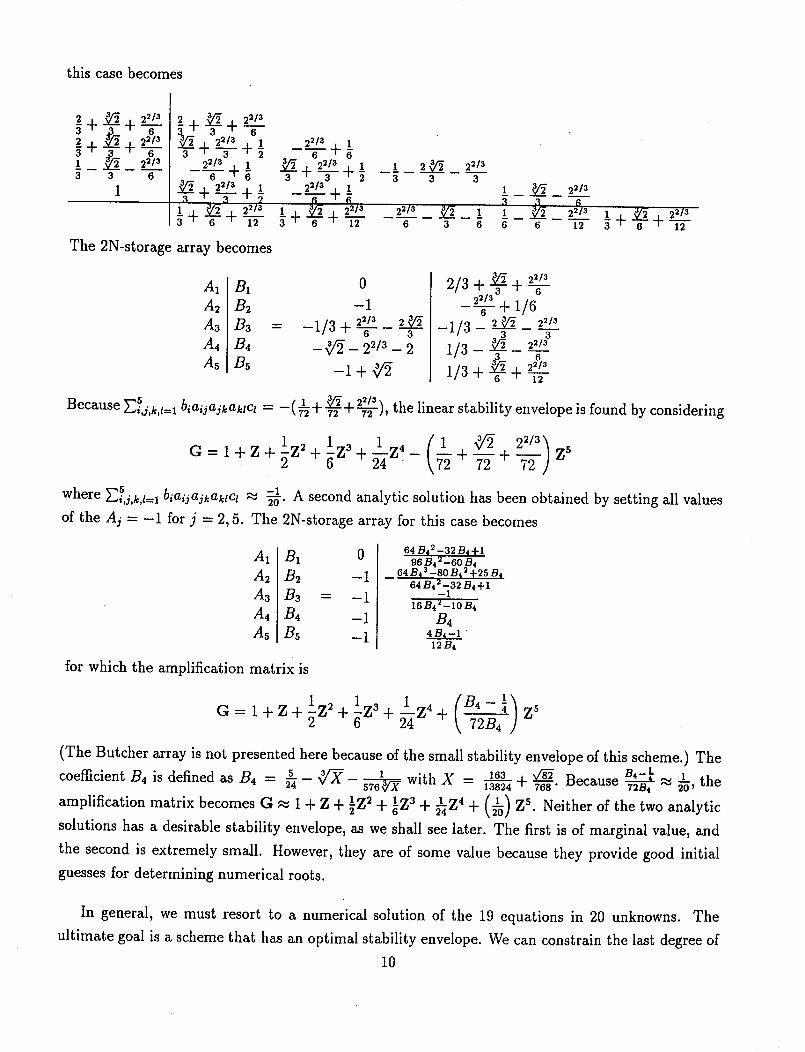
this casebecomes

_-+ _" + 22/-A

3 _ 2&2+ + --c1 -- 22/33 3 6

1

2 4- _/2 4- 22/33-- 3 --"-C-._ 4- 2213 4- 1

2213 4- 1

__ 4- 221__A3+ I_

i'_ j _._3_. 221323-- 6 -- 12

2213 1

._ 4- 2213 _ 13 ----]---_

22/3 4_ 1

--_-- _I_4. _/_ + 22133 -- 6 -- 12

The 2N-storage array becomes

2213

6

2_" 22/33 3

____

___ __ _____3 6 6 6

2213

2_312 1 _ 22133 + + x-T

A1 B1

A2 B2

A3 B3

A4

A5

B4

Bs

0

-1

22/3= -1/3 + 6 3

--'_- 2 2/3 -- 2

-1+_

2/3+_ +2_3+1/6

-1/3- _ 22/3

113- _ 22121/3+&+ _2_36

Because 5 1 4--_4- 22/3_ the linear stability envelope is found by considering_i,j,k,l=l biaijajkaklcl = --(__ 72 --"_'J,

1 2 1 3 1 4 (7_ "_/'2 2_--_)Z5G=l+Z+sZ +_z +_z - +-if+

where 5 - 1_i,i,k,l=a blaijajkamct _ _. A second analytic solution has been obtained by setting all values

of the Aj = -1 for j = 2, 5. The 2N-storage array for this case becomes

A1 B1

A2 B2

A3 B3 =

A4 B4

A5 B5

for which the amplification matrix is

0

-I

-I

-I

-i

64 B42-32 B 4 +1

96 B42_60 B4-- 64 B 43 -80 B 4 z + 25 B 4

64 B42.._ 32 B4 + I

16 B4 2_ 10 B4

B44_.__=t '12 B4

G=I+Z+_Z + Z3+_-Z +\ 72B4

(The Butcher array is not presented here because of the small stability envelope of this scheme.) The

5 4/X- ' ,s_ ,mcoefficient B4 is defined as B4 = 2_ - _ with X = _ + Because _ _, the13824 768 " 72B4

_m,,i_ic_tio.m_trixb_om_,_ _ _+Z+_Z'+_Z_+_Z"+ (_)Z'.Neithorofthetwo=_'y_icsolutions has a desirable stability envelope, as we shall see later. The first is of marginal value, and

the second is extremely small. However, they are of some value because they provide good initial

guesses for determining numerical roots.

In general, we must resort to a numerical solution of the 19 equations in 20 unknowns. The

ultimate goal is a scheme that has an optimal stability envelope. We can constrain the last degree of

10

freedomin the generalsystemby demandingthat the resultingschemebe optimal, whichproducesa systemwith 20equationsand 20unknowns.

To definetheoptimal constraint,webeginwith theamplificationmatrix for the (5,4)RK scheme,which is givenby

) ( ) ( )\i,j----1 i,j,k--I i,j,k,l=l

A particular scheme can be defined as being optimal when its stability envelope encompasses a

useful portion of the complex plane that is as large as possible for a particular choice of the complex

matrix Z. This definition of optimality is problem dependent and depends on the structure of the

eigenvalues of the system of ODE's being integrated.

We now focus specifically on hyperbolic and parabolic partial differential equations (PDE's), for

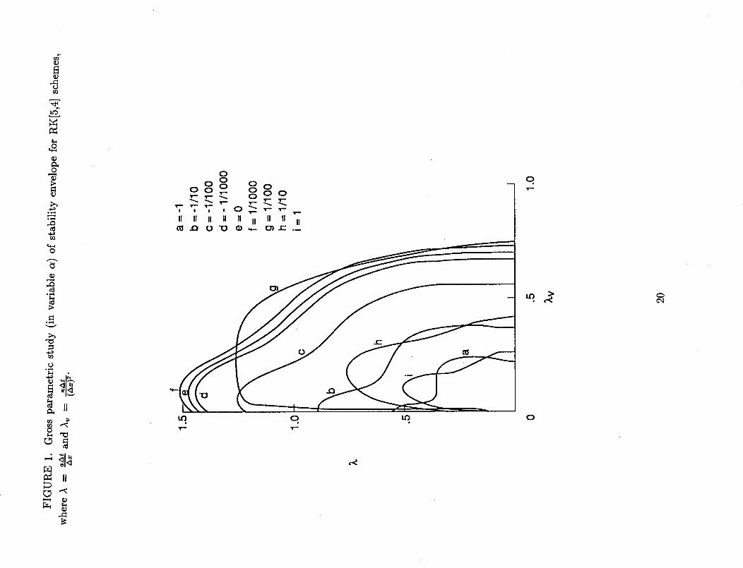
which the (5,4) 2N-storage RK schemes will be advantageous. A model equation that produces

an eigenstructure representative of the equations of fluid mechanics is Ut ÷ aU, = aUxx. If we

choose spatial operators for the Ux and U** terms, this equation reduces to a system of ODE's.

The complex matrix Z can now be interpreted to represent combinations of the inviscid and viscous

stability characteristics. Figure 1 shows a parametric study of the stability envelope as a function

of the CFL number (A--at, th and the viscous CFL number (A = oat_--_-,/ (a_)2/, as determined from the

amplification matrix G. Regions toward the origin represent stable regions for the scheme, and the

upper right portion of the plot represents the unstable regions. The spatial operator used for both the

inviscid and viscous operators was the sixth-order compact scheme [7]; however, similar conclusions

could have been reached with a Second-order or a Fourier method. (See the appendix for more5

details.) The parameter a is defined as a = _.i,.i,kd=l blaijajt, aktct. By adjusting -1 < a < 1, large

stability envelopes are obtained for values of a _ 0. Figure 2 shows a more refined plot of values

1 <a< 128--'6-- -- i_" Note that all curves have a similar structure but that no one curve simultaneously

maximizes the inviscid (imaginary axis) and viscous (real axis) stability limits. Further inspection

1 • the viscous stability limit occursreveals that the maximum inviscid stability occurs at _ = 3'

at c_ _ 2-_" The value c_ = _ provides a compromise between the two extremes. Caution should

be exercised in using values of oL near _ because the inviscid stability limit in the case of very

small viscous CFL values may change dramatically with small changes in a. Figure 3 shows the

stability limits for the (3,3) RK scheme, the (4,4) RK scheme, and three (5,4) l'tK schemes that are

functions of the parameter a. Figure 3 illustrates why the analytic schemes presented earlier do not

-1have desirable stability characteristics. The stability envelope for the analytic case a _ _8 is about

half the size of the optimal a = _0A-6;the analytic case a _ _ has a vanishingly small inviscid

stability limit.

The optimal value a = _ is used to provide the 20th nonlinear equation in 20 unknowns. The

11

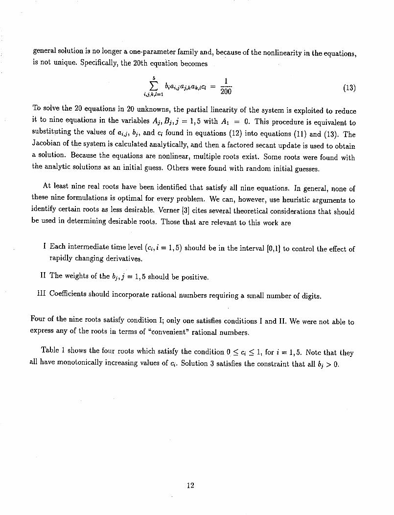
generalsolutionisno longera one-parameter family and, because of the nonlinearity in the equations,

is not unique. Specifically, the 20th equation becomes

5 1biaijaLkak,lct = _ (13)

ij,k,l=l 200

To solve the 20 equations in 20 unknowns, the partial linearity of the system is exploited to reduce

it to nine equations in the variables Ai, Bi, j = 1, 5 with A1 = 0. This procedure is equivalent to

substituting the values of ai,j, bj, and ci found in equations (12) into equations (11) and (13). The

Jacobian of the system is calculated analytically, and then a factored secant update is used to obtain

a solution. Because the equations are nonlinear, multiple roots exist. Some roots were found with

the analytic solutions as an initial guess. Others were found with random initial guesses.

At least nine real roots have been identified that satisfy all nine equations. In general, none of

these nine formulations is optimal for every problem. We can, however, use heuristic arguments to

identify certain roots as less desirable. Verner [3] cites several theoretical considerations that should

be used in determining desirable roots. Those that are relevant to this work are

I Each intermediate time level (c_, i = 1, 5) should be in the interval [0,1] to control the effect of

rapidly changing derivatives.

II The weights of the bj,j = 1,5 should be positive.

III Coefficients should incorporate rational numbers requiring a small number of digits.

Four of the nine roots satisfy condition I; only one satisfies conditions I and II. We were not able to

express any of the roots in terms of "convenient" rational numbers.

Table 1 shows the four roots which satisfy the condition 0 < c; < 1, for i = 1, 5. Note that they

all have monotonically increasing values of ci. Solution 3 satisfies the constraint that all bj > O.

12

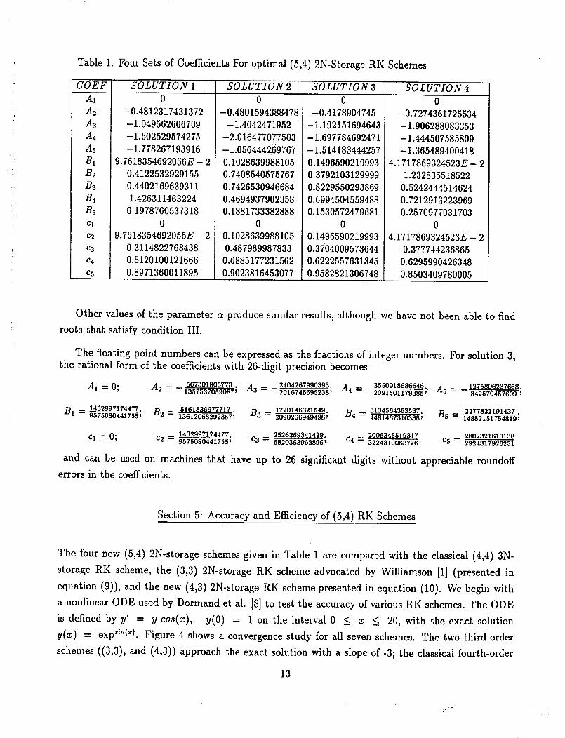
Table 1. Four Sets of Coefficients For optimal (5,4) 2N-Storage RK Schemes

COEF

Ax

A2

A3

A4

As

B1

B2

B3B4

B5

c1

C2

c3

(:4

C5

SOLUTION 1 SOLUTION 2 SOLUTION 3 SOLUTION 40

-0.4812317431372

-1.049562606709

-1.602529574275

-1.778267193916

9.7618354692056E - 2

0.4122532929155

0.4402169639311

1.426311463224

0.1978760537318

0

9.7618354692056E - 2

0.3114822768438

0.5120100121666

0.8971360011895

0

-0.4801594388478

-1.4042471952

-2.016477077503-1.056444269767

0.1028639988105

0.74085405757670.7426530946684

0.4694937902358

0.1881733382888

0

0.1028639988105

0.487989987833

0.6885177231562

0.9023816453077

0

-0.4178904745

-1.192151694643

-1.697784692471

-1.514183444257

0.1496590219993

0.3792103129999

0.8229550293869

0.6994504559488

0.1530572479681

0

0.1496590219993

0.3704009573644

0.6222557631345

0.9582821306748

0

-0.7274361725534

-1.906288083353

-1.444507585809

-1.365489400418

4.1717869324523E - 2

1.232835518522

0.5242444514624

0.7212913223969

0.2570977031703

0

4.1717869324523E - 2

0.377744236865

0.6295990426348

0.8503409780005

Other values of the parameter a produce similar results, although we have not been able to find

roots that satisfy condition III.

The floating point numbers can be expressed as the fractions of integer numbers. For solution 3,the rational form of the coefficients with 26-digit precision becomes

A1 = 0; A2 --_ 567301805773. A3 = _2404267990393. A4 = 3550918686646. As --_ 1275806237668.1357537059087, 2016746695238_ 2091501179385_ 842570457699,

BI = 1432997174477. B2 -- 5161836677717. B3 -- 1720146321549. B4 -" 3134564353537.9575080441755, 13612068292357, 2090206949498' 44814673103381

2277821191437n= _ •14882151754819'

1432997174477. 2526269341429. 2006345519317. 2802321613138Cl "0; C2 -_ 9575080441755' C3: 6820363962896'" C4 _ 32243100637761 C5 ---_ 2924317926251

and can be used on machines that have up to 26 significant digits without appreciable roundoff

errors in the coefficients.

Section 5: Accuracy and Efficiency of (5,4) RK Schemes

The four new (5,4) 2N-storage schemes given in Table 1 are compared with the classical (4,4) 3N-

storage RK scheme, the (3,3) 2N-storage RK scheme advocated by Williamson [1] (presented in

equation (9)), and the new (4,3) 2N-storage RK scheme presented in equation (10). We begin with

a nonlinear ODE used by Dormand et al. [8] to test the accuracy of various RK schemes. The ODE

is defined by y' = y cos(x), y(0) = 1 on the interval 0 _< x < 20, with the exact solution

y(x) = exp sin(x). Figure 4 shows a convergence study for all seven schemes. The two third-order

schemes ((3,3), and (4,3)) approach the exact solution with a slope of -3; the classical fourth-order

13

(4,4) scheme and the four (5,4) schemes approach the exact solution with a slope of -4. Note that the

(3,3) scheme is more accurate than the (4,3) scheme (Williamson claims the (3,3) scheme is optimal

in terms of error) and that all (5,4) schemes are more accurate than the (4,4) scheme. Relatively

little difference exists between the four (5,4) solutions, and none of the (5,4) schemes is uniformly

optimal over the entire range of the refinement study in terms of error.

A second nonlinear test problem is used to establish problem-dependent trends. The ODE is

defined by y' = y n sin n-l(x)cos(x), y(0) = 1 on the interval 0 _< x _< 20, with the exact solution

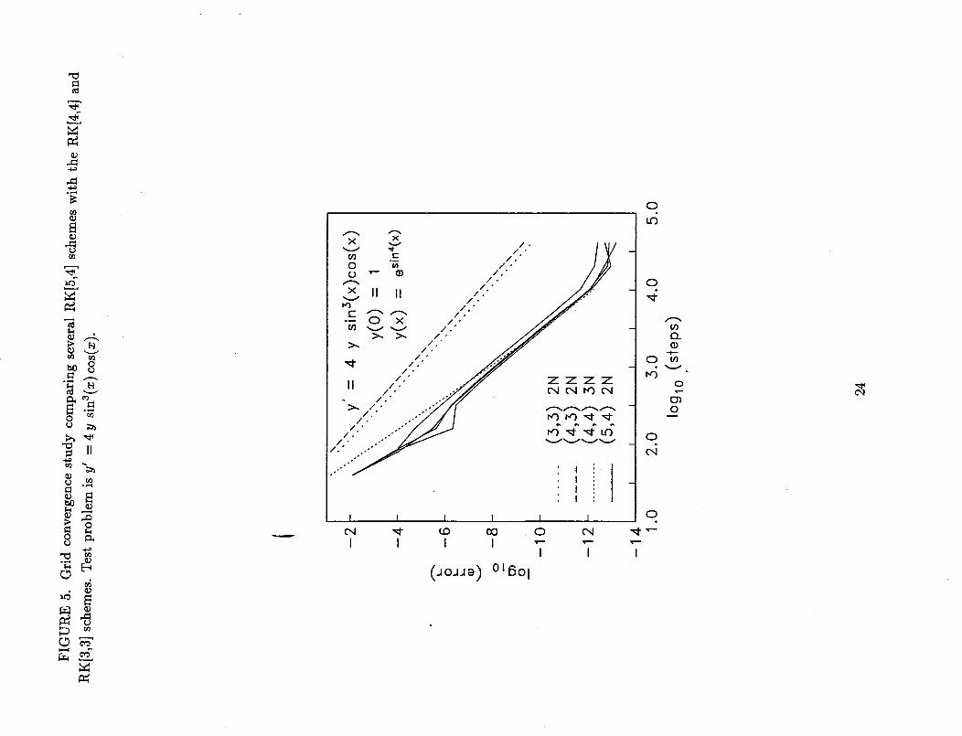
y(x) = expSin"(*), where the exponent n is n = 4. Figure 5 shows a convergence study for all seven

of the schemes. The convergence rates for the 2N-storage schemes are consistent with the theoretical

predictions, but the conventional (4,4) scheme converges at a rate that approaches -5. This rate

cannot generally be expected. If the four (5,4) 2N-storage schemes are compared between the two

nonlinear problems, solution 3 and solution 1 are most accurate in the first and second problems,

respectively. No clear advantage is evident for using any particular one of the four (5,4) 2N-storage

schemes.

This study verifies the nonlinear accuracy of the newly developed 2N-storage schemes for ODE's.

Note that in both test problems, Williamson's (3,3) scheme is more accurate and requires one-third

fewer function evaluations than the (4,3) scheme, although no attempt was made to optimize the

(4,3) schemes in terms of error. The (5,4) schemes are more accurate than the conventional (4,4) lZK

scheme in the first problem and more accurate over a significant portion of the second problem. The

(5,4) schemes appear to be more adversely affected by roundoff errors than the conventional (4,4)

scheme.

Our second problem is the solution of the linear hyperbolic equation defined by

Ou Ou

O---t+ Ox - O, 0<x<l,t_>0

u(O,t) = sin27r(-t), t > 0

u(x,O) = sin2_'(x), 0 < x_< 1

(14)

(15)

(16)

The exact solution is

u(x,t) = sin2_r(x-t), O_<x_<l,t>_O

and is a model for the class of problems that the (5,4) 2N-storage schemes were developed to integrate.

Equations (14) through (16) are solved with the same four RK schemes used in the nonlinear test

problems; specifically, the (3,3) and (4,3) third-order RK schemes and the (4,4) and (5,4) RK schemes.

In all cases, the spatial operator used is the sixth-order compact scheme developed by Carpenter et

hi. [7] and shown to be formally sixth-order accurate. The physical boundary condition is imposed

14

by solving the differentiatedboundary condition on the boundary with the RK procedure. This

techniquewasshownby Carpenteret al. [9] to yield a fourth-order temporally accurateprocedure.

Specifically,the boundary condition is d3u(O,t)/dt 3. = gin(t), where g is the physical boundary

condition at the inflow plane. The CFL that governs the stability of the hyperbolic problem is a

function of the temporal advancement and the spatial discretization used. Table 1 in the appendix

compares the inviscid CFL's and the viscous stability limits of the (3,3), (4,4), and (5,4) RK schemes

with various spatial operators, including the sixth-order compact spatial operator.

After grid refinement with a vanishingly small CFL, all schemes recover the theoretical spatial

sixth-order accuracy. On a specific grid, temporal refinement showed fourth-order temporal accuracy.

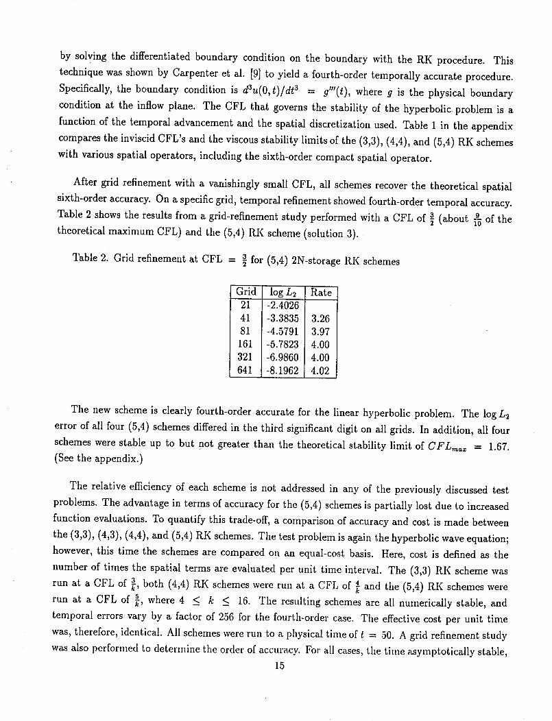
Table 2 shows the results from a grid-refinement study performed with a CFL of _ (about _ of the

theoretical maximum CFL) and the (5,4) RK scheme (solution 3).

a for (5,4) 2N-storage RK schemesTable 2. Grid refinement at CFL =

G_d logL2 Rate-2.4026

41 -3.3835 3.26

81 -4.5791 3.97

161 -5.7823 4.00

321 -6.9860 4.00

641 -8.1962 4.02

The new scheme is clearly fourth-order accurate for the linear hyperbolic problem. The log L2

error of all four (5,4) schemes differed in the third significant digit on all grids. In addition, all four

schemes were stable up to but not greater than the theoretical stability limit of CFLmax = 1.67.

(See the appendix.)

The relative efficiency of each scheme is not addressed in any of the previously discussed test

problems. The advantage in terms of accuracy for the (5,4) schemes is partially lost due to increased

function evaluations. To quantify this trade-off, a comparison of accuracy and cost is made between

the (3,3), (4,3), (4,4), and (5,4) R.K schemes. The test problem is again the hyperbolic wave equation;

however, this time the schemes are compared on an equal-cost basis. Here, cost is defined as the

number of times the spatial terms are evaluated per unit time interval. The (3,3) RK scheme was

run at a CFL of a 4 and the (5,4) R.K schemes were_, both (4,4) RK schemes were run at a CFL of

run at a CFL of 5_., where 4 < k < 16. The resulting schemes are all numerically stable, and

temporal errors vary by a factor of 256 for the fourth-order case. The effective cost per unit time

was, therefore, identical. All schemes were run to a physical time of t = 50. A grid refinement study

was also pcrformed to determine the order of accuracy. For all cases, the time _ymptotically stable,

15

sixth-ordercompactspatialoperator [7]wasusedwith the boundaryconditionsthat werepreviouslydescribed.

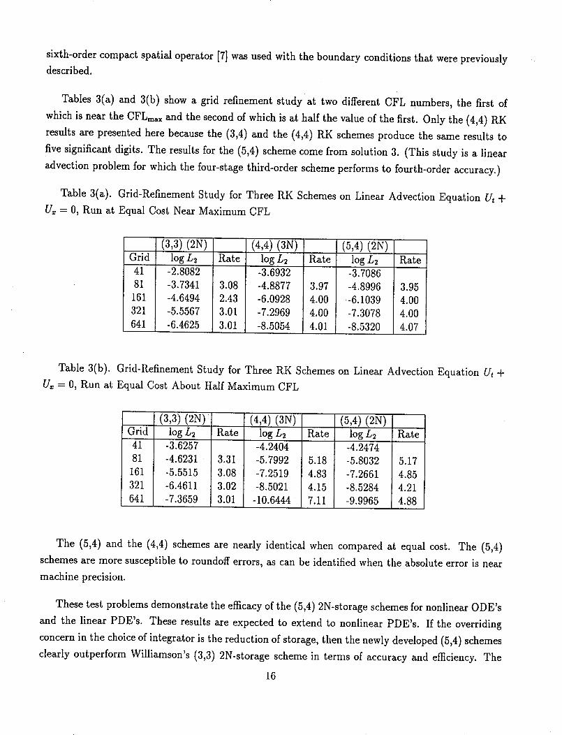
Tables3(a) and 3(b) showa grid refinementstudy at two different CFL numbers,the first of

which is nearthe CFLmaxand the secondof which is at half the valueof the first. Only the (4,4)RKresultsare presentedherebecausethe (3,4) and the (4,4) RK schemesproducethe sameresults to

five significantdigits. The resultsfor the (5,4) schemecomefrom solution 3. (This study is a linear

advectionproblemfor which the four-stagethird-order schemeperformsto fourth-orderaccuracy.)

Table 3(a). Grid-RefinementStudy for Three RK Schemeson Linear Advection Equation Ut +

Ux = 0, Run at Equal Cost Near Maximum CFL

(3,3) (2N) (4,4) (3N) (5,4) (2N)

Grid log L2 Rate log L2 Rate log L2

41 -2.8082 -3.6932 -3.7086

81 -3.7341 3.08 -4.8877 3.97 -4.8996

161 -4.6494 2.43 -6.0928 4.00 -6.1039

321 -5.5567 3.01 -7.2969 4.00 -7.3078

641 -6.4625 3.01 -8.5054 4.01 -8.5320

Rate

3.95

4.00

4.00

4.07

Table 3(b). Grid-Refinement Study for Three RK Schemes on Linear Advection Equation Ut +

U, = 0, Run at Equal Cost About Half Maximum CFL

(3,3)(2N)

Grid logL2

41 -3.6257

81 -4.6231

161 -5.5515

321 -6.4611

641 -7.3659

Rate

3.31

3.08

3.02

3.01

(4,4) (3N)

log L=

-4.2404

-5.7992

-7.2519

-8.5021

-10.6444

(5,4) (2N)

Rate log L2

-4.2474

5.18 -5.8032

4.83 -7.2661

4.15 -8.5284

7.11 -9.9965

Rate

5.17

4.85

4.21

4.88

The (5,4) and the (4,4) schemes are nearly identical when compared at equal cost. The (5,4)

schemes are more susceptible to roundoff errors, as can be identified when the absolute error is near

machine precision.

These test problems demonstrate the efficacy of the (5,4) 2N-storage schemes for nonlinear ODE's

and the linear PDE's. These results are expected to extend to nonlinear PDE's. If the overriding

concern in the choice of integrator is the reduction of storage, then the newly developed (5,4) schemes

clearly outperform Williamson's (3,3) 2N-storage scheme in terms of accuracy and efficiency. The

16

accuracyper unit cost is comparablewith that of the standardfour-stagefourth-order (4,4) RKscheme.

Conclusions

Several new five-stage fourth-order (5,4) Runge-Kutta (RK) schemes are derived that require only two

storage locations. Two of the schemes have analytic coefficients that facilitate simple implementation,

but neither have desirable stability characteristics. A particular scheme is identified (by numerically

solving the nonlinear equations) which has the desirable efficiency characteristics for hyperbolic and

parabolic initial (boundary) value problems. In the inviscid and viscous limits, this new (5,4) 2N-

storage RK scheme has greater accuracy for a given step size and has a larger allowable stability

domain than the (3,3) 2N-storage RK scheme advocated by Williamson. The new (5,4) RK scheme

is comparable with the standard (4,4) RK scheme in terms of accuracy to work ratio and is nearly

as efficient in an absolute sense. Numerical tests are presented that verify these results on nonlinear

ordinary differential equations (ODE's) and linear hyperbolic equations.

Acknowledgments

The second author would like to acknowledge financial support provided while in residence at NASA

Langley Research Center, Theoretical Flow Physics Branch, under contract NAG-l-l193.

References

[1] Williamson, J.H., "Low-storage Runge-Kutta schemes," J. Comp. Phys., 35, 48 (1980).

[2] Fyfe, D.J., "Economical evaluation of Runge-Kutta formula," Math. Comp., 20, 392 (1966).

[3] Verner, J.H., "Explicit Runge-Kutta Methods with Estimates of the Local Truncation Error,"

SIAM J. Numer. Anal., 15 (1978), pp. 772-790.

[4] Sharp, P.W. and Smart, E., "Explicit Runge-Kutta Pairs with One More Derivative Evaluation

than the Minimum," SIAM J. Sci. Comput., 14, 2 (1993), pp. 338-348.

[5] Butcher, J.C., The Numerical Analysis of Ordinary Differential Equations: Runge-Kutta and

General Linear Methods, John Wiley _ Sons, Chichester (1987).

[6] Skeel, R.D., "Thirteen Ways to Estimate Global Error," Numer. Math., 48, (1986), pp. 1-20.

17

[7] Carpenter,M.H., Gottlieb, D., and Abarbanel,S., "The Stability of NumericalBoundaryTreat-

mentsfor CompactHigh-OrderFinite-DifferenceSchemes,"J. Comp. Phy, 108, 2, (1993), pp.

272-295.

[8] Dormand, J.R., and Prince, P.J., "A Family of embedded Runge-Kutta formulae," J. Comp.

Appl. Math., 6, 1, (1980), pp. 19-26.

[9] Carpenter, M.H., Gottlieb, D., Abarbanel, S. and Don, W.-S. " The Theoretical Accuracy of

Runge-Kutta Time Discretizations for the Initial Boundary Value Problem: A Careful Study

of the Boundary Error," NASA-CR-191561, ICASE Report No. 93-83, Dec. 1993. Submitted to

SIAM Journal of Numerical Analysis.

Appendix I

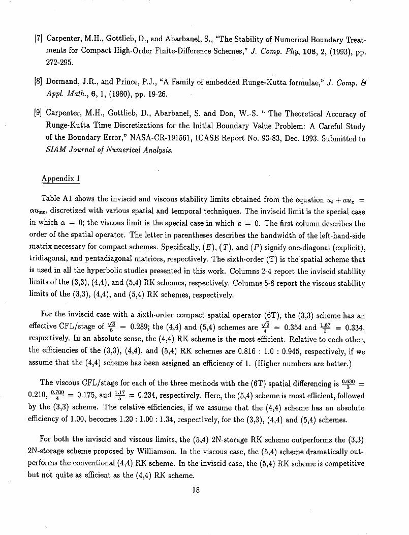
Table A1 shows the inviscid and viscous stability limits obtained from the equation ut + au, =

au**, discretized with various spatial and temporal techniques. The inviscid limit is the special case

in which a = 0; the viscous limit is the special case in which a = 0. The first column describes the

order of the spatial operator. The letter in parentheses describes the bandwidth of the left-hand-side

matrix necessary for compact schemes. Specifically, (E), (T), and (P) signify one-diagonal (explicit),

tridiagonal, and pentadiagonal matrices, respectively. The sixth-order (T) is the spatial scheme that

is used in all the hyperbolic studies presented in this work. Columns 2-4 report the inviscid stability

limits of the (3,3), (4,4), and (5,4) RK schemes, respectively. Columns 5-8 report the viscous stability

limits of the (3,3), (4,4), and (5,4) RK schemes, respectively.

For the inviscid case with a sixth-order compact spatial operator (6T), the (3,3) scheme has an

effective CFL/stage of _ = 0.289; the (4,4) and (5,4) schemes are v_ = 0.354 and 1.6__27= 0.334,4 5

respectively. In an absolute sense, the (4,4) RK scheme is the most efficient. Relative to each other,

the efficiencies of the (3,3), (4,4), and (5,4) RK schemes are 0.816 : 1.0 : 0.945, respectively, if we

assume that the (4,4) scheme has been assigned an efficiency of 1. (Higher numbers are better.)

The viscous CFL/stage for each of the three methods with the (6T) spatial differencing is 0.s3.__.._o3

0.210, 0.70._____04-- 0.175, and _ = 0.234, respectively. Here, the (5,4) scheme is most efficient, followed

by the (3,3) scheme. The relative efficiencies, if we assume that the (4,4) scheme has an absolute

efficiency of 1.00, becomes 1.20 : 1.00 : 1.34, respectively, for the (3,3), (4,4) and (5,4) schemes.

For both the inviscid and viscous limits, the (5,4) 2N-storage RK scheme outperforms the (3,3)

2N-storage scheme proposed by Williamson. In the viscous case, the (5,4) scheme dramatically out-

performs the conventional (4,4) RK scheme. In the inviscid case, the (5,4) RK scheme is competitive

but not quite as efficient as the (4,4) RK scheme.

18

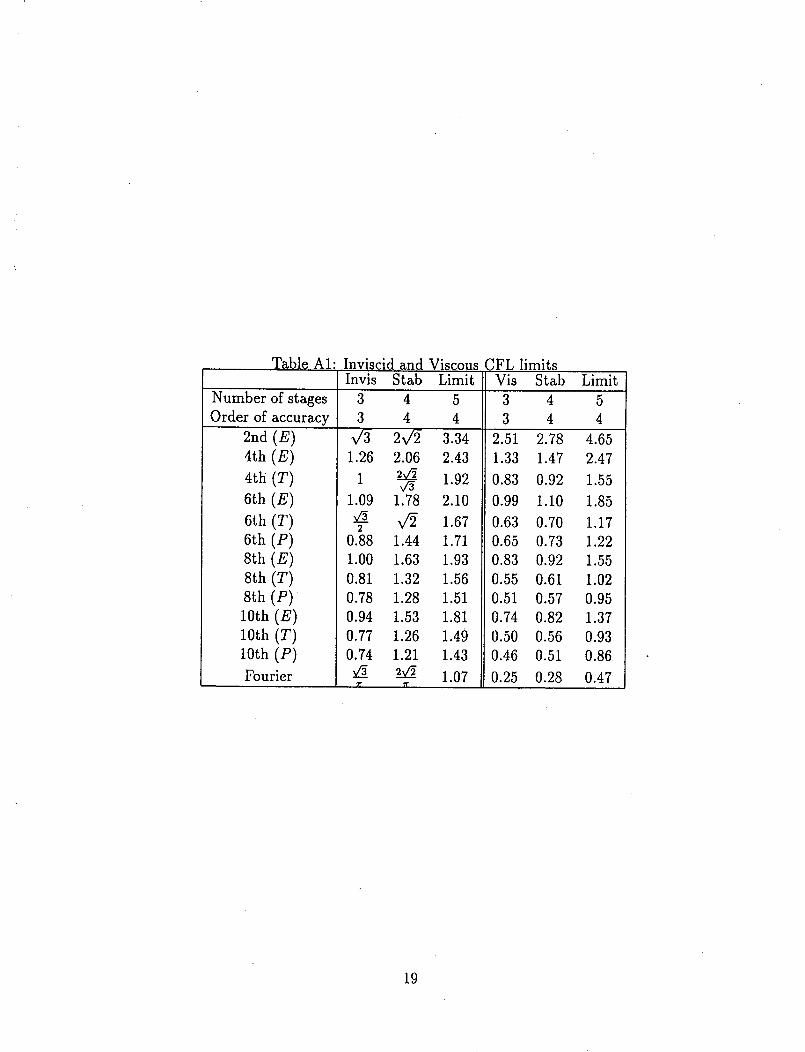
Table AI: Inviscid and ViscousCFL limitsInvis Stab Limit Vis Stab

Number of stagesOrder of accuracy

2nd(E)4th (E)

4th (T)

6th (E)

6th (T)6th (P)

8th (E)

8th (T)8th (P)

10th (E)

10th (T)

10th (P)

Fourier

3 4 5

3 4 4

v_ 2v_ 3.341.26 2.06 2.43

l _ 1.92

1.09 1.78 2.10

v_ v/_ 1.672

0.88 1.44 1.71

1.00 1.63 1.93

0.81 1.32 1.56

0.78 1.28 1.51

0.94 1.53 1.81

0.77 1.26 1.49

0.74 1.21 1.43

v_ 2v_ 1.077f

Limit

3 4 5

3 4 4

2.78

1.47

0.92

1.10

0.70

0.73

0.92

0.61

0.57

0.82

O.56

0.51

O.28

2.51

1.33

0.83

0.99

0.63

0.65

0.83

0.55

0.51

0.74

0.50

0.46

0.25

4.65

2.47

1.55

1.85

1.17

1.22

1.55

1.02

0.95

1.37

0.93

0.86

0.47

19

0

;;h.1'-4

o,'-t,.c

u'J

0

°,-i

r.n

c_

0

r.o

u_ o u.) o

FIGURE 2. Refined parametric study (in variable a) of stability envelope for RK[5,4] schemes.

2.0RK (5, 4)

a = 1/120

b-- 1/160

c = 1/200

d -- 1/240

e -- 1/280

0 .5

a b ¢

_,V

1.0

d

1.5

21

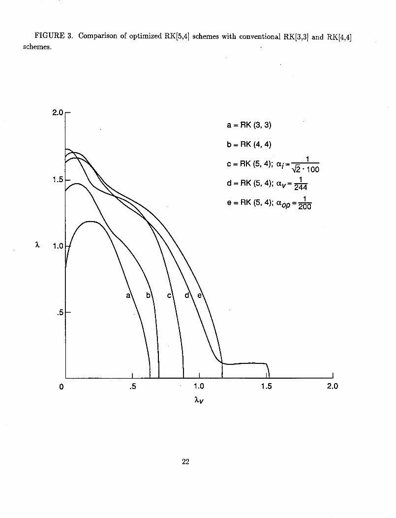
FIGURE 3. Comparison of optimized RK[5,4] schemes with conventional RK[3,3] and RK[4,4]

schemes.

2"0 /_ a = RK (3, 3)

/ b = RK (4, 4)

1

c = RK (5, 4); a I -._-_. 100

1d = RK (5, 4); av= 24_

1e = RK (5, 4); aop ='_'0

a

0 .5 1.5

I

2.0

22

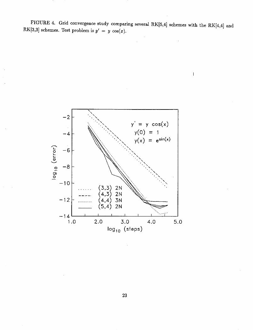
FIGURE 4. Grid convergence study comparing several RK[5,4] schemes with the RK[4,4] and

RK[3,3] schemes. Test problem is y' = y cos(x).

Ok.

{D

O

O

-2

-4

-6

-8-

-10 -

-12 -

-141.0

\\

\• \

:,, ,,"',\ y'= y cos(x)

_k-, "_,_\ y(O)--I

_,., "\,.'-,,\\ y(x) = e sin(x)• .. ".. \\

_. "\\•.... -. ,_,,,,

",. " . ,\\

.... _" ",:

.......... (4,4) ,3N

(5,4) 2N

f I f I I I """1

2.0 3.0 4.0

Ioglo (steps)

5.0

23

0_

°,_

t_ t_

0

o_._

0

_e3

/ °

/ °/°°

/,,/o°

/,/o"

/°/.

/#°/.

/"/o

/,/.°

/,/ °

I I I t I

C'M _ cO 09 0 ¢'q

' ' _ ' T T(JoJJ_) °L6ol

0

IF)

0

4

O_

0

o

0"_0

0

0

"_t'--

I

c_

REPORT DOCUMENTATION PAGE Form ApprovedOMB No. 0704-0188

Publicreportingburdenforthiscollectionofinformationis estimated to average1hourperresponse,includingthetime forreviewinginstructions,searchingexistingdatasources,gatheringand maintainingthedataneeded,andcompleting end reviewingthe collectionof information. Sendcommentsregardingthis burdenestimateor anyotheraspectofthiscollectionof information,includingsuggestionsfor reducingthisburden,toWashingtonHeadquartersServices.Directoratefor InformationOperationsand Reports,1215JeffersonDavisHighway,Suite1204, Arlington,VA 22202-4302,andtothe OfficeofManagementandBudget,PaperworkReductionProject(0704-0188),Washington,DC 20503.

1. AGENCY USE ONLY (Leave blank) 2. REPORT DATE

June 1994

4. TITLE AND SUBTITLE

Fourth-Order 2N-Storage Runge-Kutta Schemes

6. AUTHOR(S)

Mark H. Carpenter

Christopher A. Kennedy

7. PERFORMINGORGANIZATIONNAME(S)ANDADDRESS(ES)

NASA Langley Research CenterHampton, VA 23681-0001

9. SPONSORINGI MONITORINGAGENCYNAME(S)ANDADDRESS(ES)

National Aeronautics and Space AdministrationLangley Research Center

Hampton, VA 23681

3. REPORTTYPEANDDATESCOVEREDTechnical Memorandum5. FUNDINGNUMBERS

505-70-62-13

8. PERFORMING ORGANIZATIONREPORT NUMBER

10. SPONSORING/MONITORINGAGENCY REPORT NUMBER

NASA TM-109112

11. SUPPLEMENTARY NOTES

Carpenter: Langley Research Center, Hampton, VA.Kennedy: University of California at San Diego, LaJolla, CA.

12a. DISTRIBUTION / AVAILABILITY STATEMENT

Unclassified - Unlimited

Subject Category: 02

12b. DISTRIBUTION CODE

13. ABSTRACT (Maximum 200 words)

A family of five-stage fourth-order Runge-Kutta schemes is derived; these schemes required only two storage

locations. A particular scheme is identified that has desirable efficiency characteristics for hyperbolic andparabolic initial (boundary) value problems. This scheme is competitive with the classical fourth-order method

(high-storage) and is considerably more efficient and accurate than existing third-order low-storage schemes.

14. SUBJECT TERMS

Runge-Kutta, low storage, fourth-order

17. SECURITY CLASSIFICATIONOF REPORT

Unclassified

18. SECURITY CLASSIFICATIONOF THIS PAGE

Unclassified

NSN 7540-01-280-5500

19. SECURITY CLASSIFICATIONOF ABSTRACT

Unclassified

15. NUMBER OF PAGES

25

16. PRICE CODE

A03

20. LIMITATION OF ABSTRACT

Unlimited

Standard Form 298 (Rev. 2-89)Prescribedby ANSIStd. Z39-18298-102