Bull Earthquake EngDOI 10.1007/s10518-013-9482-z

ORIGINAL RESEARCH PAPER

Fourier spectral- and duration models for the generationof response spectra adjustable to different source-,propagation-, and site conditions

Sanjay Singh Bora · Frank Scherbaum ·Nicolas Kuehn · Peter Stafford

Received: 21 November 2012 / Accepted: 28 June 2013© Springer Science+Business Media Dordrecht 2013

Abstract One of the major challenges related with the current practice in seismic hazardstudies is the adjustment of empirical ground motion prediction equations (GMPEs) to dif-ferent seismological environments. We believe that the key to accommodating differencesin regional seismological attributes of a ground motion model lies in the Fourier spectrum.In the present study, we attempt to explore a new approach for the development of responsespectral GMPEs, which is fully consistent with linear system theory when it comes to adjust-ment issues. This approach consists of developing empirical prediction equations for Fourierspectra and for a particular duration estimate of ground motion which is tuned to optimizethe fit between response spectra obtained through the random vibration theory frameworkand the classical way. The presented analysis for the development of GMPEs is performed onthe recently compiled reference database for seismic ground motion in Europe (RESORCE-2012). Although, the main motivation for the presented approach is the adjustability andthe use of the corresponding model to generate data driven host-to-target conversions, evenas a standalone response spectral model it compares reasonably well with the GMPEs ofAmbraseys et al. (Bull Earthq Eng 3:1–53, 2005), Akkar and Bommer (Seismol Res Lett81(2):195–206, 2010) and Akkar and Cagnan (Bull Seismol Soc Am 100(6):2978–2995,2010).

Keywords Ground motion prediction equation · Fourier amplitude spectrum · Duration ·Random vibration theory · Response Spectrum

1 Introduction

Estimation of potential ground motion intensity measures (GMIMs), such as peak groundacceleration or response spectra for a given scenario, is one of the major goals in engi-

S. S. Bora (B) · F. Scherbaum · N. KuehnInstitute of Earth and Environmental Science, University of Potsdam, Potsdam, Germanye-mail: sanjay.singh@geo.uni-potsdam.de

P. StaffordDepartment of Civil and Environmental Engineering, Imperial College London, London, UK

123

Bull Earthquake Eng

neering seismology, and in seismic hazard studies. Often in applications like probabilisticseismic hazard assessments (PSHA) empirical ground motion prediction equations (GMPEs)are employed for estimating potential GMIMs at a site of interest from all the relevant sce-narios. Also, other methods like numerical simulations are usually found to be less reliableat high frequencies (f > 1 Hz), which are of significant interest in seismic design practices.The GMPEs are derived through a regression algorithm over a selected set of data com-prising GMIMs, such as peak ground acceleration or response spectral ordinates, against achosen set of predictor variables such as magnitude, source -to -site distance, site conditioninformation. Essentially, GMPEs describe a conditional distribution of a selected GMIM interms of a median value and a logarithmic standard deviation (σ ) which is a measure of thespread of the observed data around the median and is supposed to capture aleatory variabilityof ground motion generation. In the recent past many efforts have been made to developempirical GMPEs based on recorded data sets, in different tectonic environments. The mainobjective has been to capture the scaling of ground motion with respect to earthquake source,path, and site parameters; and also to confine the complexity in the functional form of theregression model. A compendium of GMPEs developed so far can be found in Douglas (2003,2011).

There are many regions, particularly the intra-plate regions across the globe which areseismically active, but have a paucity of recorded data which is typically insufficient togenerate endemic empirical GMPEs. For performing seismic hazard studies in such regionsusual practice is to consider GMPEs from some other regions. The selection of a particularGMPE to a study region is not straightforward and is often based on a subjective decisionof the hazard analyst. Not accounting for changes in regional seismological attributes likesource, path and site condition can often lead to an unrealistic estimate of ground motion. Toaddress this issue, Campbell (2003, 2004) has suggested the use of “host-to-target” adjustmentfactors when GMPEs are “imported” from some other region to a region of the study whichhe terms as the “host”and “target” region respectively. These adjustment factors are usuallycalculated as the ratio of stochastically simulated response spectral ordinates (Boore 2003)for both the regions. However, the concept of accommodating differences in seismologicalparameters is rooted in the Fourier spectrum of ground motion which is not related linearly tothe response spectrum. Hence it is still an issue of debate to which extent adjustment factorsbased on response spectral ratios can fully accommodate the true difference in seismologicalparameters. Moreover, response spectrum is an outcome of a nonlinear process while Fourierspectrum is considered as the outcome of a linear process in terms of the transfer-functionsof the constituent seismological attributes of ground motion like source, path and site.

The characteristics of Fourier amplitude spectra (FAS) of ground motion are often modeledtheoretically in terms of seismological parameters like stress drop, kappa, quality factor andcrustal amplification with respect to Brune’s source model (Brune 1970). This model of theFAS coupled with a spectrum of random phase angles to model high frequency ground motionhas been thoroughly investigated (Hanks and McGuire 1981; Boore 2003). This technique ofsimulating time histories has proven to be a simple yet reliable method of realizing groundmotions of engineering interest and has been extensively used for predicting ground motionsin many regions of the world (see Boore 2003, Table 5).

The discussion in the last two paragraphs implies that the issues related with the adjustmentof GMPEs can be addressed in a physically consistent manner if the GMPEs are developed forFAS. However, for seismic resistant design of a structure one needs to know the response ofthe structure to the potential input ground motion. Moreover, as stated earlier the relationshipbetween the response spectrum of a single degree of freedom (SDOF) system and the FASof the input ground motion is not linear. Possibly, this is the reason that mostly the GMPEs

123

Bull Earthquake Eng

found in literature are for predicting the response spectral ordinates. On the contrary, veryfew empirical equations have been found for the prediction of FAS. The main efforts whichinvolve the development of Fourier spectral GMPEs are, Trifunac (1976), McGuire (1978),Atkinson and Mereu (1992), Sokolov et al. (2000), Stafford (2006) and Stafford et al. (2006).

In the present article we attempt to address the issues discussed in the last paragraph whichare related with the use of FAS for developing GMPEs and consequently to estimate responsespectral ordinates. The important issue is the relation of FAS of the input ground motionwith the response of a SDOF system. Boore (2003) has demonstrated the use of randomvibration theory (RVT) for simulating ground motion with an underlying theoretical FASof the ground motion. This method of computing a response spectrum essentially combinesthe FAS with a predetermined estimate of ground motion duration. A similar approach forthe fast computation of response spectrum by combining the FAS and duration of groundmotion through RVT has been demonstrated by Reinoso et al. (1990) and Jaimes et al. (2006).Originally, the work of Vanmarcke and Lai (1980) relates the duration of ground motion withthe FAS and the peak value of the motion through the theory of stationary Gaussian randomfunctions. The details of the method are discussed in the following sections. However, onehas to realize that the calculation of response spectral ordinates within the RVT frameworkdepends on one more parameter which is the duration of the input ground motion. This isanother parameter of strong ground motion which has received relatively little attention in thepast as far as the development of prediction equations is concerned. Recently, the studies ofKempton and Stewart (2006) and Bommer et al. (2009) involve the development of empiricalequations for predicting different measures of ground motion duration.

Essentially, the method we propose in this article for estimating the response spectral ordi-nates which can be adjusted in different source-, propagation- and site conditions is based ona similar approach to that discussed in the last paragraph. Mainly, it involves the developmentof GMPEs for Fourier spectral ordinates and a particular measure of ground motion duration;and in subsequent steps the estimates obtained from the two GMPEs are combined within theRVT framework to obtain the response spectral ordinates. As mentioned earlier, calculationof response spectral ordinates in RVT depends upon the duration of the ground motion (Boore2003). However, there are multiple definitions for ground motion duration each of which maybe suitable for a particular application (Bommer and Martinez-Pereira 1999). A key and newelement of our approach is that we determine the individual ground motion durations notfrom the seismogram but treat it as a variable used to minimize the mismatch (squared error)between the observed and RVT estimated response spectrum (by spectral moments). Therequired Fourier spectrum is calculated from the observed acceleration record, further detailsof the method will be discussed in the next two sections.

This study is a part of the SeIsmic Ground Motion Assessment (SIGMA) project whichinvolves the development of new and updated GMPEs for Europe and the neighboringregions. Therefore the presented analysis for the development of the GMPEs is performedon the recently compiled RESORCE-2012 strong motion database Akkar et al. (2013) acrossEurope, the Mediterranean and the Middle East. The selected dataset for our analysis consistsof 1,232 records from 369 earthquakes. Section 7 of this article will demonstrate that themodel developed in the present study compares reasonably well with the previous publishedmodels for the region (Ambraseys et al. 2005; Akkar and Bommer 2010; Akkar and Cagnan2010) and that the model can therefore be regarded as a stand-alone model. However, themain motivation for the presented approach is to generate a ground motion model which isadjustable to different source-, propagation- and site conditions. Our approach of generatingresponse spectra from the combination of duration and FAS of ground motion facilitates oneto perform such adjustments easily and in a physically consistent manner. This has been

123

Bull Earthquake Eng

demonstrated in Sect. 7.3 of this article by considering a simple example in which one makesan adjustment to account for differences in the parameter kappa.

Additionally, we believe that our approach can also be used to directly generate host-to-target region adjustment factors for response spectra. Usually, the response spectral ratiobased adjustment factors (Campbell 2003, 2004) are calculated for a reference magnitude anddistance scenario which ignores the potential dependence of those ratios on predictor variableslike magnitude, distance and Vs30. When using these single scenario based adjustment factors,the quality of the adjustment will depend upon how well the scenario will match the scenariocoming from the hazard disaggregation. If the hazard disaggregation results in several relevantscenarios, the use of single scenario adjustment factors is not justified at all.

Finally, the analysis presented in this study should primarily be interpreted as an initialattempt towards the development of a physically consistent approach for addressing adjust-ment issues with GMPEs.

2 Essence of the approach

The basis of developing GMPEs in this article lies within the RVT framework which hasbeen successfully used by Boore (2003) to predict the response spectral ordinates of a SDOFoscillator for an input ground motion of finite duration. Typically, the calculation of responsespectral ordinates through RVT involves the use of the FAS, Y(MW , R, Vs30, f) and anindependent estimate of ground motion duration (Dgm); the equations involved in the calcu-lation will be discussed in the following subsection. The FAS of ground motion at a particularfrequency, f, for a given magnitude (MW )-distance (R) scenario is expressed in terms of itsconstituent seismological attributes like source (E), path (P) and site (S) as,

Y (MW , R, V s30, f ) = E(MW , f )P(R, f )S( f ) (1)

The amplitude and shape of each term in Eq. 1 are controlled by various seismologicalparameters. For example, the source spectrum is determined by the seismic moment M0

(consequently MW ) and the stress parameter; the path effect is determined by geometricalspreading and quality factor (Q) of the medium; and similarly the site effects are typicallycontrolled by kappa and the shear wave velocity (V s30) beneath the recording station.

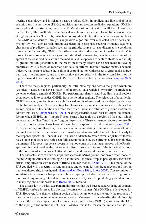
Hence, the presented approach of estimating response spectral ordinates is essentially atwo-step method, first the empirical equations are developed for the FAS and Dgm of groundmotion; and second, the median predictions from both the equations are combined throughRVT to obtain the median response spectral ordinates corresponding to a SDOF system. Aschematic representation of the approach is depicted in Fig. 1.

In Fig. 1 Y(MW , R, Vs30, f) and Dgm(MW , R, Vs30) are the median predicted FASand median predicted Dgm respectively for the set of predictor variables, magnitude (MW ),source-to-site distance (R) and site condition (Vs30) scenario; and ymax (MW , R, Vs30, fosc)

Fig. 1 Schematic representation of the presented approach

123

Bull Earthquake Eng

is the predicted maximum response of the SDOF system corresponding to a particular oscil-lator frequency, fosc. We do not include a nonlinear intensity parameter in the site responseterm in our empirical equations just to keep the analysis simple given that this is the firstinvestigation of its kind. However, the inclusion of this nonlinearity in the site response termdepends upon whether it can be constrained by the given dataset.

2.1 Random vibration theory

Originally, RVT was used by Cartwright and Longuet-Higgins (1956) to predict the expectedpeak height of ocean waves from spectral characteristics of a continuous record of sea waveheights. Earthquake records can not be considered as pure stationary stochastic signals,nevertheless the ground motions simulated by using the RVT method have been shown to bereasonably comparable with the observed data in various parts of the world. Essentially, RVTprovides an estimate of the ratio of the peak motion (ymax ) to the root-mean squared motion(yrms), where Parseval’s theorem is used to obtain yrms from the Fourier spectrum of theground motion. For details of the theory, the reader is referred to Cartwright and Longuet-Higgins (1956) and Boore (2003); however, the relevant equations used in the present analysisare discussed in what follows. According to Boore (2003) the ratio of the peak motion to rmsmotion can be expressed as follows

ymax

yrms= f (Nz, Ne), (2)

in the above equation Ne and Nz are the number of extrema and zero crossings which arerelated to the frequencies of extrema crossing (fe), zero crossing (fz) and duration of groundmotion Dgm as

Ne = 2 fe( fosc)Dgm, (3)

Nz = 2 fz( fosc)Dgm, (4)

where the frequencies are given by

fe( fosc) = 1

2π

(m2

m0

) 12

, (5)

fz( fosc) = 1

2π

(m4

m2

) 12

, (6)

in Eqs. 5 and 6, mk, k = 0, 2, 4 are the spectral moments of the squared spectral amplitude.These are the key quantities in RVT and are defined for any integer k as

mk = 2

∞∫0

(2π f )k |Y (MW , R, f, fosc)|2d f, (7)

in Eq. 7 Y(MW , R, f, fosc) is the FAS of the response of the SDOF system which is a mul-tiplication of FAS, Y(MW , R, VS30, f) of input ground motion and the instrument transferfunction, I(f, fosc).

In Eq. 2 yrms is calculated as

yrms( fosc) =√

m0

Drms. (8)

123

Bull Earthquake Eng

In the above equation, for the calculation of yrms a different duration estimate (Drms) hasbeen used which essentially incorporates the extension in actual Dgm because of the oscillatorresponse. Since m0 gives an estimate of the total energy present in the signal (here oscillatorresponse), it is assumed that the oscillator may continue to oscillate beyond the actual durationof the input ground motion because of the inertia of the system; and hence the total energy maybe distributed beyond the actual duration of the ground motion. This rationale of extension induration cannot be used for the calculation of Nz and Ne because the amplitudes, generatedbeyond the duration of input ground motion are not expected to produce the highest peak.To account for this extension in duration due to the oscillator response, Boore and Joyner(1984) proposed one equation as follows

Drms = Dgm + D0

(γ n

γ n + α

), (9)

where γ = Dgm fosc; and D0 = 1/(2πζ fosc) is defined as the oscillator duration. Here ζ isused to denote the damping ratio of a SDOF oscillator. The values of the constants n and α

were suggested as 3 and 1/3 respectively. Based on the comparison between the time domainand RVT results, Liu and Pezeshk (1999) suggest n = 2 and

α =[

2π

(1 − m2

1

m0m2

)] 12

(10)

Recently Boore and Thompson (2012) proposed a new model for the calculation of Drms asfollows

Drms

Dgm=

(c1 + c2

1 − ηc3

1 + ηc3

) [1 + c4

2πζ

(η

1 + c5ηc6

)c7]

(11)

here in Eq. 11 η = D0/Dgm .

3 Data

For the present analysis, the data have been taken from the RESORCE-2012 strong-motiondatabase compiled in the framework of the SIGMA project. This entire database comprisesthe 5,115 processed recordings from 1,685 events recorded at strong motion stations aroundEurope, the Mediterranean region, the Middle East and some parts of central Asia as well.However, we do not consider the entire database for our analysis in this article. It is a usualpractice in studies involved with the GMPE development to select a dataset based on criteriaadopted by the equation developer. Our general approach for selecting the dataset is to includeall the earthquakes and records except,

(1) events for which moment magnitude is not reported,(2) events for which MW < 4.0,(3) any event which is not representative of a shallow crustal event i.e. hypocentral depth

> 30 km,(4) any event with no information of the style of faulting,(5) any record not having either of the two horizontal components,(6) any record for which the Joyner–Boore distance is not reported,(7) any record for which the shear-wave velocity Vs30 is not reported,

123

Bull Earthquake Eng

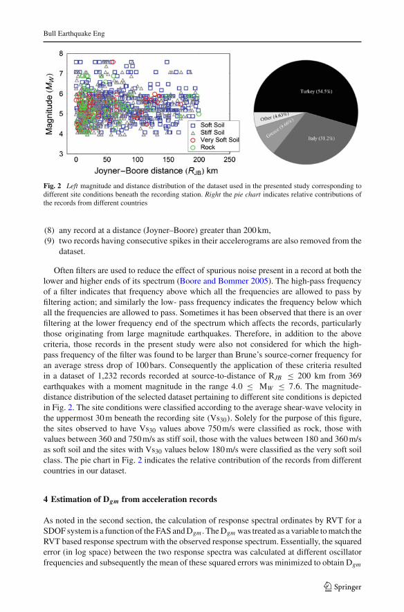
Fig. 2 Left magnitude and distance distribution of the dataset used in the presented study corresponding todifferent site conditions beneath the recording station. Right the pie chart indicates relative contributions ofthe records from different countries

(8) any record at a distance (Joyner–Boore) greater than 200 km,(9) two records having consecutive spikes in their accelerograms are also removed from the

dataset.

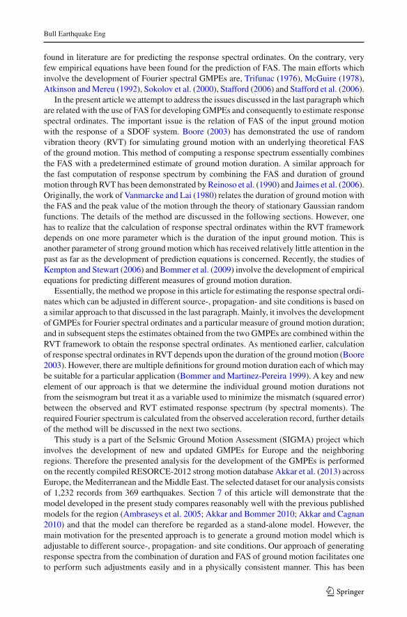
Often filters are used to reduce the effect of spurious noise present in a record at both thelower and higher ends of its spectrum (Boore and Bommer 2005). The high-pass frequencyof a filter indicates that frequency above which all the frequencies are allowed to pass byfiltering action; and similarly the low- pass frequency indicates the frequency below whichall the frequencies are allowed to pass. Sometimes it has been observed that there is an overfiltering at the lower frequency end of the spectrum which affects the records, particularlythose originating from large magnitude earthquakes. Therefore, in addition to the abovecriteria, those records in the present study were also not considered for which the high-pass frequency of the filter was found to be larger than Brune’s source-corner frequency foran average stress drop of 100 bars. Consequently the application of these criteria resultedin a dataset of 1,232 records recorded at source-to-distance of RJB ≤ 200 km from 369earthquakes with a moment magnitude in the range 4.0 ≤ MW ≤ 7.6. The magnitude-distance distribution of the selected dataset pertaining to different site conditions is depictedin Fig. 2. The site conditions were classified according to the average shear-wave velocity inthe uppermost 30 m beneath the recording site (Vs30). Solely for the purpose of this figure,the sites observed to have Vs30 values above 750 m/s were classified as rock, those withvalues between 360 and 750 m/s as stiff soil, those with the values between 180 and 360 m/sas soft soil and the sites with Vs30 values below 180 m/s were classified as the very soft soilclass. The pie chart in Fig. 2 indicates the relative contribution of the records from differentcountries in our dataset.

4 Estimation of Dgm from acceleration records

As noted in the second section, the calculation of response spectral ordinates by RVT for aSDOF system is a function of the FAS and Dgm . The Dgm was treated as a variable to match theRVT based response spectrum with the observed response spectrum. Essentially, the squarederror (in log space) between the two response spectra was calculated at different oscillatorfrequencies and subsequently the mean of these squared errors was minimized to obtain Dgm

123

Bull Earthquake Eng

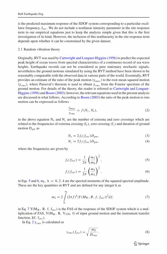
Fig. 3 Plots indicating the closeness of the match between observed response spectrum and RVT calculatedresponse spectrum optimized for a particular value of Dgm

from an acceleration trace. For the calculation of RVT based response spectrum, initiallythe response of the SDOF system was computed for a particular oscillator frequency (fosc)

using the FAS of the input ground motion, Y(MW , R, f), and the instrument transfer functionI(f, fosc) i.e. Y(MW , R, f, fosc) = Y(MW , R, f) I(f, fosc). In subsequent steps this responseof the SODF system was used to calculate the spectral moments, Drms, yrms and finallythe ymax (maximum response) at a particular fosc. The Boore and Thompson (2012) model(Eq. 11) was used to relate the ground motion duration (Dgm) with the root-mean square

123

Bull Earthquake Eng

duration (Drms). This calculation of RVT based response spectrum was implemented in aMathematica code which contains various subroutines for calculating spectral moments, rmsduration (Drms), rms motion (yrms) and response spectral ordinates (ymax ) from moments.The Fourier spectrum of the ground motion was calculated from the acceleration trace usinga multitaper spectral algorithm in which the orthonormal Hermite functions were used as thedata tapers (Simons et al. 2003). The closeness of match between the observed response spec-trum and the optimized RVT calculated response spectrum is depicted in Fig. 3 for differentmagnitude and distance combinations. The ground motion duration, Dgm was calculated forboth the horizontal components separately and the geometrical mean of the two was used forfurther analysis.

Considerable attention has been paid in the last decade (Boore and Bommer 2005; Akkarand Bommer 2006; Akkar et al. 2011; Douglas and Boore 2011) to the useable frequencyrange of a record, particularly for calculating the response spectral ordinates at low oscillatorfrequencies (long periods). The high-pass and low-pass frequencies of the filter used in therecord processing stage impose restrictions on the useable frequency limits of the groundmotion records for further application. Usually prediction equations derived for estimatingspectral ordinates define a useable frequency (period) range as a fraction of the high-passand low-pass frequencies. The lower and upper limit selections are based on the assumptionthat the spectral response at frequencies beyond some fraction of the filter cut-off (low-passand high-pass) is distorted by the filter roll-off, depending upon filter type and order of thefilter (Boore and Bommer 2005). For developing their GMPE, Abrahamson and Silva (1997)used the response spectral ordinates for frequencies (oscillator) greater than 1.25 times thehigh-pass frequency and less than 1/1.25 times the low-pass frequency of the filter. A similarfrequency limit was also used by Spudich et al. (1999) for deriving their GMPE. A similarapproach of limiting the frequency range for the calculation of response spectral ordinates

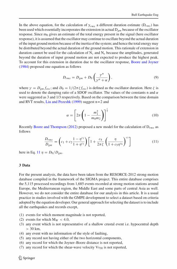
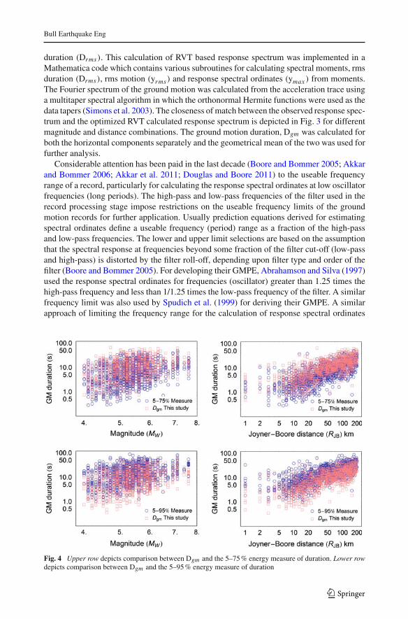
Fig. 4 Upper row depicts comparison between Dgm and the 5–75 % energy measure of duration. Lower rowdepicts comparison between Dgm and the 5–95 % energy measure of duration

123

Bull Earthquake Eng

(for both observed and RVT) has been adopted in this study. We calculate the response spectra(both observed and the moment-based) only for oscillator frequencies greater than 1.25 timesthe high-pass frequency and less than 1/1.25 times the low-pass frequency.

As we suggest a completely unique and different measure for duration, the obvious curios-ity will be about its comparability with the other measures of duration. A comparison betweenDgm computed by the procedure explained above and significant duration which is computedas the time-interval between the two specified levels (e.g.5–75 % and 5–95 %) of Arias inten-sity (Arias 1970) is depicted in Fig. 4. Both the measures of duration were computed over thedataset which is being used in the present study. Interestingly, the Dgm values are observedto be in between the two (5–75 % and 5–95 %) other measures of duration.

5 Regression model for Dgm

In the present section we develop an empirical equation for the prediction of Dgm , as one ofthe building blocks of the RVT framework. There are many other applications in engineeringseismology for which an estimate of Dgm with respect to magnitude and distance is desired,so the presented empirical relation can also be considered as one of the tools in such studies.There are limited studies found on the prediction of Dgm in terms of earthquake magnitude,distance and other seismological parameters. However, recently Kempton and Stewart (2006)and Bommer et al. (2009) have published empirical equations for the prediction of differentmeasures of ground motion duration.

In the present study we considered a simple functional form of Dgm prediction equa-tion. The basic aim was to select an equation which can capture the underlying physics ofthe process. According to the theoretical considerations the duration of ground motion isattributed mainly to the duration of the shear pulse generated at the source which is furtherelongated during the course of wave propagation from source to site because of the scatteringand reflection effects (Boore 2003; Atkinson and Boore 1995; Hermann 1985). The durationof this shear pulse generated at the source is mainly determined by the rupture dynamics atthe source, but in the RVT framework it is commonly assumed to be the reciprocal of theBrune corner frequency (Hanks and McGuire 1981; Boore 2003) which essentially dependsupon the earthquake size.

Therefore in the present study, a regression equation similar to the one proposed byBommer et al. (2009) was considered,

ln(Dgm) = c0 + c1 MW + (c2 + c3 MW ) ln√

R2JB + c2

4 + c5 ln V s30 + η + ε. (12)

In the above equation Dgm (s) is the geometric mean of the duration estimated from thetwo horizontal components; MW is the moment magnitude; RJB(km) is the closest distancefrom the recording site to the surface projection of the rupture plane; and Vs30(m/s) is thetime-averaged shear wave velocity in the upper 30 m of the soil profile beneath the recordingsite. The coefficients of Eq. 12 were determined by employing a random effects regressionalgorithm as suggested by Abrahamson and Youngs (1992). In this algorithm the residualsare separated into between-event (η) and within-event terms (ε); and are assumed to benormally distributed with zero mean, with the standard deviation τ and φ respectively. Thetotal standard deviation associated with the median duration for an average (geometric mean)horizontal component is calculated as follows,

σ =√

τ 2 + φ2 (13)

123

Bull Earthquake Eng

Table 1 Coefficients associated with median ground motion duration for an average horizontal component

c0 c1 c2 c3 c4 c5 τ φ σ

−2.4805 0.7907 1.3711 −0.1297 5.3554 −0.3445 0.3179 0.4809 0.5765

5.1 Regression results

The coefficients associated with the median Dgm for an average horizontal (geometric mean)component are presented in Table 1. The estimated coefficients through regression in Eq. 12were found statistically significant to well beyond the 99 % confidence limit.

5.2 Residuals

In order to assess the robustness and stability of the presented empirical equation we examinethe residuals by plotting them against the three predictor variables, magnitude, distance andVs30. Figure 5 indicates that between-event residuals do not exhibit any bias with respect tothe magnitude; and similarly within-event residuals also do not indicate any bias with respectto RJB and Vs30. Figure 6 depicts the Q–Q plots for the between-event and within-eventresiduals, and it can be observed that Q–Q plots are relatively straight with respect to standardnormal plot, indicating the validation of the assumption of log normal distribution for Dgm .

Fig. 5 Residual plots for Dgm

123

Bull Earthquake Eng

Fig. 6 Q–Q Plots of normalized between-event and within-event residuals associated with Dgm

5.3 Median predicted Dgm

In the present study, we use a completely different measure of duration, Dgm , neverthelesswe compare the median predicted Dgm obtained from the current empirical equation withthe other estimates of duration obtained from the studies of Kempton and Stewart (2006)and Bommer et al. (2009). The other two studies use a different measure of duration whichis based on the time interval-between the two specified levels (e.g. 5–75 % and 5–95 %) ofArias intensity (Arias 1970). The comparison of median predicted Dgm with the other twoduration estimates and their scaling with respect to magnitude and distance is depicted inFig. 7. The first notable feature that can be observed from Fig. 7 is that the shape of scaling ofmedian Dgm with respect to magnitude and distance predicted by current empirical equation

Fig. 7 Plots depicting the comparison of Dgm predicted by current empirical model with those from Kemptonand Stewart (2006) and Bommer et al. (2009). Upper row indicates the comparison with the 5–75 % energymeasure of duration model from the other two studies. Lower row indicates the same for 5–95 % energymeasure of duration

123

Bull Earthquake Eng

is similar to that of Kempton and Stewart (2006) and Bommer et al. (2009). This trend inscaling can be expected when we use a similar functional form for the empirical equation.However, it is not surprising that the predicted Dgm values are not observed to be identicalwith those obtained from the studies of Kempton and Stewart (2006) and Bommer et al.(2009) neither for 5–95 % nor for 5–75 % energy measure of duration. In fact the Dgm valuespredicted by the current empirical equation are found in between the two other estimatesof duration. This mismatch in duration estimates can be attributed to a different measure ofduration, Dgm which was defined with a completely different purpose in mind. The otherpossible reason for this mismatch can be the use of RJB as a source to site distance metricin this study, whereas the other two studies use Rrupt . Additionally, the studies of Kemptonand Stewart (2006) and Bommer et al. (2009) use different datasets for their analysis whichmay also lead to the difference in the duration estimates.

6 Regression model for FAS

As mentioned earlier, the calculation of response spectral ordinates through RVT dependsupon both the FAS and a duration measure of ground motion. Hence in this section wedevelop an empirical equation, for the prediction of Fourier spectral ordinates. However,ever since the advent of spectrum techniques in engineering seismology, it has remaineda challenge to predict the FAS of ground motion on the basis of a chosen set of predictorvariables such as earthquake magnitude, distance from source to site, local soil conditionsbeneath the recording site. On the other hand, many empirical GMPEs have been publishedfor the response spectrum of ground motion. Studies predicting the FAS are rare, but include(Trifunac 1976; McGuire 1978; Atkinson and Mereu 1992; Sokolov et al. 2000; Stafford2006; Stafford et al. 2006).

Analytically the far field FAS of ground motion acceleration is typically explained withrespect to Brune’s source spectrum which is further modified by attenuation along the wavepropagation path and the amplification (or diminution) effects because of the near surface soilproperties beneath the recording site. Hence an ideal functional form of the empirical equationcan be thought of as involving all the seismological parameters which determine the shapeof the source spectrum and the subsequent path and site effects on it e.g. stress drop, kappa,quality factor, site amplification. However inclusion of a large number of predictor variablesoften leads to the non-convergence of the regression process. Therefore in the present studyan attempt was to consider a simple empirical equation, yet one that is powerful enough tocapture the scaling with commonly used parameters like magnitude, source-to-site distanceand Vs30. The functional form of the empirical equation used for the regression is as follows,

ln(Y ( f )) = c0 + c1 MW + c2 M2W + (c3 + c4 MW ) ln

(√R2

JB + c25

)− c6

√R2

JB + c25

+ c7 ln V s30 + η + ε. (14)

In Eq. 14, Y is the geometric mean of Fourier spectral amplitude from both the horizontal com-ponents at frequency f. The definition of predictor variables remains the same as mentionedin the previous section. At each frequency the between-event error term, η, and within-eventerror term, ε, were assumed to be normally distributed with zero means and standard devi-ation τ and φ respectively; and the total standard deviation, σ , is calculated as describedin Eq. 13. A frequency-by-frequency regression was performed using the Eq. 14. The samerandom effects regression algorithm of Abrahamson and Youngs (1992) was employed forthe purpose.

123

Bull Earthquake Eng

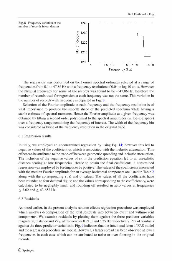
Fig. 8 Frequency variation of thenumber of records in our dataset

The regression was performed on the Fourier spectral ordinates selected at a range offrequencies from 0.1 to 47.86 Hz with a frequency resolution of 0.04 in log 10 units. Howeverthe Nyquist frequency for some of the records was found to be <47.86 Hz, therefore thenumber of records used for regression at each frequency was not the same. This variation inthe number of records with frequency is depicted in Fig. 8.

Selection of the Fourier amplitude at each frequency and the frequency resolution is ofvital importance to produce the smooth shape of the predicted spectrum while having astable estimate of spectral moments. Hence the Fourier amplitude at a given frequency wasobtained by fitting a second order polynomial to the spectral amplitudes (in log-log space)over a frequency range containing the frequency of interest. The width of the frequency binwas considered as twice of the frequency resolution in the original trace.

6.1 Regression results

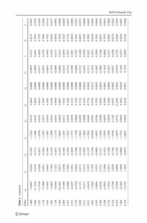
Initially, we employed an unconstrained regression by using Eq. 14; however this led tonegative values of the coefficient c6 which is associated with the inelastic attenuation. Thiseffect can be attributed to the trade-off between geometric spreading and inelastic attenuation.The inclusion of the negative values of c6 in the prediction equation led to an unrealisticdistance scaling at low frequencies. Hence to obtain the final coefficients, a constrainedregression was employed by forcing c6 to be positive. The values of the coefficients associatedwith the median Fourier amplitude for an average horizontal component are listed in Table 2along with the corresponding τ, φ and σ values. The values of all the coefficients havebeen rounded to four decimal digits; and the values corresponding to the coefficient c6 werecalculated to be negligibly small and rounding off resulted in zero values at frequencies≤ 3.02 and ≥ 43.652 Hz.

6.2 Residuals

As noted earlier, in the present analysis random effects regression procedure was employedwhich involves decomposition of the total residuals into between- event and within-eventcomponents. We examine residuals by plotting them against the three predictor variablesmagnitude, distance and Vs30 at frequencies 0.21, 1 and 5.25 Hz respectively. Plot of residualsagainst the three predictor variables in Fig. 9 indicates that the functional form of FAS modeland the regression procedure are robust. However, a larger spread has been observed at lowerfrequencies in each case which can be attributed to noise or over filtering in the originalrecords.

123

Bull Earthquake Eng

Tabl

e2

Coe

ffici

ents

asso

ciat

edw

ithth

em

edia

nFo

urie

rsp

ectr

alor

dina

tes

for

anav

erag

eho

rizo

ntal

com

pone

nt

F(H

z)c 0

c 1c 2

c 3c 4

c 5c 6

c 7τ

φσ

0.10

0−1

3.58

943.

0455

−0.1

154

−2.7

737

0.29

5110

.491

20.

0000

−0.3

858

0.98

941.

1866

1.54

50

0.11

0−1

4.30

253.

3713

−0.1

429

−2.7

525

0.29

4210

.275

60.

0000

−0.4

041

0.98

461.

1662

1.52

63

0.12

0−1

4.99

953.

6979

−0.1

728

−2.7

449

0.29

829.

9717

0.00

00−0

.421

20.

9818

1.13

831.

5032

0.13

2−1

5.73

944.

0381

− 0.2

056

−2.7

357

0.30

499.

4501

0.00

00−0

.438

40.

9764

1.10

701.

4761

0.14

5−1

6.53

984.

4127

−0.2

407

−2.6

919

0.30

518.

8897

0.00

00−0

.464

70.

9617

1.07

961.

4458

0.15

8−1

7.55

774.

8491

−0.2

786

−2.5

885

0.29

378.

3605

0.00

00−0

.493

00.

9513

1.05

001.

4168

0.17

4−1

8.29

855.

1976

−0.3

104

−2.5

058

0.28

627.

7911

0.00

00−0

.519

10.

9384

1.02

201.

3874

0.19

1−1

8.94

605.

4917

−0.3

365

−2.3

867

0.27

357.

0006

0.00

00−0

.546

50.

9107

1.00

041.

3529

0.20

9−1

9.62

165.

7895

−0.3

606

−2.2

156

0.24

916.

2668

0.00

00−0

.577

30.

8703

0.99

641.

3229

0.22

9−2

0.10

045.

9827

−0.3

749

−2.0

452

0.22

395.

6505

0.00

00−0

. 592

30.

8456

0.99

491.

3057

0.25

1−2

0.17

606.

0539

−0.3

800

−1.8

924

0.20

145.

1643

0.00

00−0

.612

50.

8307

0.99

161.

2936

0.27

5−1

9.71

345.

9875

−0.3

752

−1.8

042

0.19

054.

7998

0.00

00−0

.645

60.

8160

0.99

611.

2876

0.30

2−1

9.27

775.

9970

−0.3

820

−1.7

794

0.18

974.

8453

0.00

00−0

.682

50.

8084

0.99

311.

2805

0.33

1−1

8.81

585.

8887

−0.3

722

−1.6

822

0.17

504.

6418

0.00

00−0

.699

50.

7719

0.97

851.

2463

0.36

3−1

8.25

195.

7524

−0.3

597

−1.5

961

0.15

924.

7354

0.00

00−0

.711

60.

7424

0.94

551.

2022

0.39

8−1

8.15

475.

8771

−0.3

701

−1.5

030

0.13

674.

8020

0.00

00−0

.753

10.

7128

0.92

121.

1647

0.43

7−1

8.15

246.

0126

−0.3

855

−1.4

552

0.12

804.

6014

0.00

00−0

.784

00.

6759

0.91

191.

1351

0.47

9−1

7.21

095.

7850

−0.3

676

−1.4

295

0.12

184.

5252

0.00

00−0

.803

60.

6489

0.91

151.

1189

0.52

5−1

5.90

465.

3736

−0.3

310

−1.3

570

0.10

964.

5698

0.00

00−0

.818

40.

6247

0.90

311.

0981

0.57

5−1

4.26

094.

9872

−0.3

087

−1.4

616

0.13

014 .

5482

0.00

00−0

.843

10.

6058

0.87

101.

0609

0.63

1−1

4.17

825.

0554

−0.3

140

−1.3

194

0.10

773.

5710

0.00

00−0

.893

50.

5686

0.85

531.

0270

0.69

2−1

3.27

314.

8753

−0.2

936

−1.1

335

0.07

353.

7381

0.00

00−0

.970

90.

5438

0.84

881.

0080

0.75

9−1

3.30

904.

8635

−0.2

884

−1.0

358

0.05

293.

7749

0.00

00−0

.958

80 .

5291

0.82

950.

9839

0.83

2−1

2.06

934.

6464

−0.2

752

−1.1

761

0.06

534.

9231

0.00

00−0

.976

30.

5003

0.83

340.

9720

0.91

2−1

1.53

984.

5504

−0.2

693

−1.1

452

0.05

584.

4173

0.00

00−0

.986

70.

4733

0.81

070.

9387

123

Bull Earthquake Eng

Tabl

e2

cont

inue

d

F(H

z)c 0

c 1c 2

c 3c 4

c 5c 6

c 7τ

φσ

1.00

0−9

.894

74.

0356

−0.2

305

−1.2

234

0.07

194.

6044

0.00

00−0

.985

50.

4723

0.82

350.

9493

1.09

6−1

1.33

244.

5718

−0.2

731

−1.1

086

0.04

475.

0642

0.00

00−0

.988

90.

4681

0.79

520.

9228

1.20

2−1

1.07

484.

4268

−0.2

621

−1.0

789

0.03

434.

6414

0.00

00−0

.931

70.

4826

0.77

930.

9166

1.31

8−9

.700

93.

9551

− 0.2

304

−1.1

925

0.05

734.

7987

0.00

00−0

.895

10.

4754

0.78

840.

9206

1.44

5−8

.554

53.

6045

−0.1

964

−1.1

867

0.04

346.

1892

0.00

00−0

.884

50.

4493

0.79

520.

9134

1.58

5−9

.488

23.

7485

−0.2

150

−1.2

589

0.05

345.

6706

0.00

00−0

.757

80.

4355

0.80

550.

9157

1.73

8−9

.836

43.

7253

−0.2

033

−1.1

178

0.01

816.

9640

0.00

00−0

.696

90.

4173

0.80

780.

9092

1.90

5−1

0.32

873.

8977

−0.2

155

−1.0

829

0.00

396.

8807

0.00

00−0

.680

40.

4412

0.79

360.

9080

2.08

9−9

.169

83.

4760

−0.1

865

−1.1

507

0.01

137.

9165

0.00

00−0

.613

50.

4070

0.78

250.

8820

2.29

1−8

.468

63.

3983

−0.1

956

−1.3

923

0.04

388.

7463

0.00

00−0

. 571

80.

3837

0.77

360.

8635

2.51

2−8

.835

73.

4561

−0.2

029

−1.3

775

0.04

788.

1232

0.00

00−0

.550

90.

3851

0.80

100.

8888

2.75

4−8

.472

03.

0426

−0.1

560

−1.1

760

0.00

606.

7384

0.00

00−0

.466

00.

3707

0.79

410.

8763

3.02

0−6

.115

12.

6711

−0.1

416

−1.5

622

0.05

998.

7742

0.00

00−0

.533

10.

3420

0.80

570.

8753

3.31

1−5

.811

12.

2373

−0.1

022

−1.3

862

0.04

088.

1433

0.00

18−0

.424

50.

3970

0.76

290.

8600

3.63

1−6

.841

02.

3972

−0.1

197

−1.3

934

0.04

438.

7754

0.00

26−0

.311

10.

3623

0.79

020.

8693

3.98

1−7

.496

52.

1755

−0.1

190

−0.9

398

0.07

910.

4754

0.01

23−0

.327

60.

3671

0.82

460.

9026

4.36

5−5

.090

41.

9743

−0.0

989

−1.6

851

0.07

469.

3555

0.00

19−0

.266

20.

3994

0.78

910.

8844

4.78

6−6

.833

62.

3731

−0.1

271

−1.4

556

0.04

009.

9483

0.00

43−0

.206

60.

3166

0.80

170.

8619

5.24

8−6

.991

82.

3500

−0.1

423

−1.5

925

0.08

798.

5950

0.00

63−0

.161

80.

4004

0.78

750.

8834

5.75

4−7

.076

22.

2671

−0.1

290

−1.5

449

0.06

709 .

1960

0.00

66−0

.104

70.

4127

0.80

030.

9004

6.31

0−5

.279

61.

8250

−0.1

106

−1.8

768

0.11

029.

8307

0.00

62−0

.055

70.

4106

0.82

790.

9242

6.91

8−5

.939

62.

0994

−0.1

259

−1.8

979

0.07

1612

.249

50.

0036

−0.0

159

0.37

430.

8469

0.92

59

7.58

6−6

.346

41.

5696

−0.0

858

−1.7

534

0.09

798.

2853

0.00

700.

1454

0.42

770 .

8428

0.94

51

8.31

8−5

.579

11.

1852

−0.0

479

−1.6

091

0.06

958.

8244

0.00

710.

1578

0.40

290.

8764

0.96

46

123

Bull Earthquake Eng

Tabl

e2

cont

inue

d

F(H

z)c 0

c 1c 2

c 3c 4

c 5c 6

c 7τ

φσ

9.12

0−5

.407

81.

2738

−0.0

688

−1.9

276

0.11

109.

5048

0.00

680.

1868

0.42

470.

8687

0.96

70

10.0

00−6

.479

41.

5428

−0.0

953

−1.9

970

0.12

009.

7718

0.00

630.

2419

0.42

870.

8895

0.98

74

10.9

65−6

.590

81.

6179

−0.1

071

−2.0

362

0.13

448.

6308

0.00

680.

1894

0.43

470.

9206

1.01

81

12.0

23−7

.488

31.

8077

−0.1

091

−1. 8

236

0.08

118.

1970

0.00

600.

1959

0.44

150.

9270

1.02

68

13.1

83−4

.901

10.

9848

−0.0

400

−1.8

936

0.08

018.

9972

0.00

430.

1587

0.45

170.

9851

1.08

38

14.4

54−6

.152

21.

1037

−0.0

440

−1.7

934

0.05

529.

2397

0.00

520.

2691

0.46

731.

0417

1.14

17

15.8

49−7

.367

01.

6119

−0.0

915

−1.8

041

0.06

018.

2373

0.00

520.

2019

0.46

621.

1166

1.21

00

17.3

78−7

.856

51.

4200

−0.0

772

−1.8

332

0.07

246.

8253

0.00

550.

3175

0.50

211.

1350

1.24

11

19.0

55−8

.933

71.

5872

−0.0

952

−1.7

286

0.08

245.

5329

0.00

840.

3135

0.54

831.

2015

1.32

06

20.8

93−8

.605

81.

3241

−0.0

755

−1.8

117

0.09

605.

5713

0.00

970.

3705

0.53

161.

2367

1.34

61

22.9

09−8

.241

70.

9262

−0.0

461

−1.9

720

0.13

324.

2038

0.01

110.

4540

0.60

581.

2867

1.42

21

25.1

19−6

.228

00.

3037

0.01

67−2

.127

00.

1113

6.68

940.

0084

0.46

420.

6448

1.41

241.

5526

27.5

42−7

.228

60.

6209

−0.0

043

−2.2

991

0.10

807.

5397

0.00

760.

4958

0.66

601.

4693

1.61

32

30.2

00−5

.933

70.

3904

0.00

95−2

.744

20.

1479

8.27

990.

0064

0.48

230.

6817

1.55

791.

7006

33.1

13− 5

.653

40.

2973

0.03

99−2

.768

90.

1061

9.72

890.

0052

0.45

140.

7268

1.62

281.

7781

36.3

08−3

.148

9−0

.466

60.

0864

−3.2

791

0.19

439.

3862

0.00

550.

4351

0.78

721.

6494

1.82

76

39.8

11−2

.252

7−0

.623

40.

1078

−3.7

346

0.20

8910

.422

10.

0013

0.45

310.

8522

1.67

151.

8763

43.6

52−2

.211

0−0

.875

60.

1286

−4.0

071

0.24

809.

6545

0.00

000.

5080

0.99

901.

6971

1.96

93

47.8

63−3

.956

7−0

.732

20.

0964

−4.4

669

0.36

548.

9008

0.00

000.

6137

1.23

491.

7329

2.12

79

123

Bull Earthquake Eng

Fig. 9 Residual plots for FAS at different frequencies

Fig. 10 Scaling of median predicted FAS with a magnitude, b distance and c Vs30

123

Bull Earthquake Eng

Fig. 11 Scaling of Fourier spectral ordinates with respect to magnitude and distance corresponding to frequen-cies f = 0.21, 1.0 and 5.25 Hz. The predictions have been computed for the rock site condition, Vs30 = 760 m/s

6.3 Median predicted FAS

The scaling of median FAS, predicted by the current empirical equation, against magnitude,distance and Vs30 are depicted in Fig. 10. Panel (a) in Fig. 10 shows the scaling of the medianFAS with respect to magnitude; and the magnitude-corner frequency correlation is readilyvisible. Panel (b) of the same figure depicts the scaling with respect to distance. Similarlythe influence of site conditions in terms of Vs30 is depicted in panel (c) of the same figure. Itcan be observed that the amplification of spectra for softer sites peaks at lower frequenciesand that for harder rock sites it peaks at higher frequencies.

Additionally, the scaling of median FAS with respect to magnitude and distance is depictedin Fig. 11, corresponding to frequencies 0.21, 1.0 and 5.25 Hz. Figure 11 indicates that thescaling of FAS with respect to magnitude is physically consistent with observed saturationat larger magnitudes. The scaling with respect to distance is also observed to be physicallyconsistent which indicates the attenuation of seismic wave energy with distance. A slow decayrate of Fourier spectral ordinates, with respect to distance at low frequencies, particularly forlarge magnitudes can be explained by the stochastic model; the large magnitude earthquakesgenerate a larger amount of low frequency content and these low frequency signals attenuatewith a slower rate because of the lesser effect of quality factor in this frequency range. Theother possible reason can be that for larger magnitude earthquakes the source-extension maycome into the picture.

7 Response spectrum

As mentioned earlier, we calculate the response spectral ordinates through RVT by com-bining the FAS and Dgm of ground motion. Hence the median predicted response spec-trum for a particular magnitude-distance scenario is estimated by following the schemedepicted in Fig. 1. The same Mathematica code, containing the subroutines for comput-ing spectral moments, rms duration (Drms), rms motion (yrms) and the response spectrum(ymax ), was used to obtain the response spectrum. For the computation of spectral momentsmedian predicted FAS and Dgm estimates were obtained from the respective empiricalequations.

123

Bull Earthquake Eng

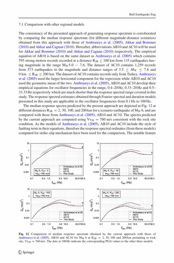
7.1 Comparison with other regional models

The consistency of the presented approach of generating response spectrum is corroboratedby comparing the median response spectrum (for different magnitude-distance scenarios)obtained from this approach with those of Ambraseys et al. (2005), Akkar and Bommer(2010) and Akkar and Cagnan (2010). Hereafter, abbreviations AB10 and AC10 will be usedfor Akkar and Bommer (2010) and Akkar and Cagnan (2010) respectively. The empiricalequation of AB10 is based on the same dataset as Ambraseys et al. (2005) which contains595 strong motion records recorded at a distance RJB ≤ 100 km from 135 earthquakes hav-ing magnitude in the range MW 5.0 − 7.6. The dataset of AC10 contains 1,259 recordsfrom 573 earthquakes in the magnitude and distance ranges of 3.5 ≤ MW ≤ 7.6 and0 km ≤ RJB ≤ 200 km. The dataset of AC10 contains records only from Turkey. Ambraseyset al. (2005) used the larger horizontal component for the regression while AB10 and AC10used the geometric mean of the two. Ambraseys et al. (2005), AB10 and AC10 develop theirempirical equations for oscillator frequencies in the range, 0.4–20 Hz, 0.33–20 Hz and 0.5–33.33 Hz respectively which are much shorter than the response spectral range covered in thisstudy. The response spectral estimates obtained through Fourier spectral and duration modelspresented in this study are applicable to the oscillator frequencies from 0.1 Hz to 100 Hz.

The median response spectra predicted by the present approach are depicted in Fig. 12 atdifferent distances RJB = 2, 30, 100, and 200 km for a scenario earthquake of MW 6, and arecompared with those from Ambraseys et al. (2005), AB10 and AC10. The spectra predictedby the current approach are computed using Vs30 = 760 m/s consistent with the rock sitecondition. As the models of Ambraseys et al. (2005), AB10 and AC10 include the style offaulting term in their equations, therefore the response spectral ordinates (from these models)computed for strike-slip mechanism have been used for the comparison. The notable feature

Fig. 12 Comparison of median response spectrum obtained by the current approach with those ofAmbraseys et al. (2005), AB10 and AC10 for MW 6 at RJB = 2, 30, 100 and 200 km pertaining to rocksite, Vs30 = 760 m/s. The dots at 100 Hz indicate the corresponding PGA values to the other three models

123

Bull Earthquake Eng

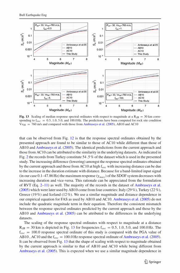
Fig. 13 Scaling of median response spectral ordinates with respect to magnitude at a RJB = 30 km corre-sponding to fosc = 0.5, 1.0, 5.0, and 100.0 Hz. The predictions have been computed for rock site conditionVs30 = 760 m/s and compared with those from Ambraseys et al. (2005), AB10 and AC10

that can be observed from Fig. 12 is that the response spectral ordinates obtained by thepresented approach are found to be similar to those of AC10 while different than those ofAB10 and Ambraseys et al. (2005). The identical predictions from the current approach andthose from AC10 can be attributed to the similarity in the underlying datasets. As indicated inFig. 2 the records from Turkey constitute 54 .5 % of the dataset which is used in the presentedstudy. The increasing difference (lowering) amongst the response spectral ordinates obtainedby the current approach and those from AC10 at high fosc with increasing distance can be dueto the increase in the duration estimate with distance. Because for a band-limited input signal(in our case 0.1–47.86 Hz) the maximum response (ymax ) of the SDOF system decreases withincreasing duration and vice-versa. This rationale can be appreciated from the formulationof RVT (Eq. 2–11) as well. The majority of the records in the dataset of Ambraseys et al.(2005) which were later used by AB10 come from four countries: Italy (29 %), Turkey (22 %),Greece (19 %) and Iceland (12 %). We use a similar magnitude and distance dependence inour empirical equation for FAS as used by AB10 and AC10. Ambraseys et al. (2005) do notinclude the quadratic magnitude term in their equation. Therefore the consistent mismatchbetween the response spectral ordinates predicted by the current approach and those by theAB10 and Ambraseys et al. (2005) can be attributed to the differences in the underlyingdatasets.

The scaling of the response spectral ordinates with respect to magnitude at a distanceRJB = 30 km is depicted in Fig. 13 for frequencies fosc = 0.5, 1.0, 5.0, and 100.0 Hz. Thefosc = 100.0 response spectral ordinate of this study is compared with the PGA value ofAB10 , AC10 and the fosc = 100.0 Hz response spectral ordinate of Ambraseys et al. (2005).It can be observed from Fig. 13 that the shape of scaling with respect to magnitude obtainedby the current approach is similar to that of AB10 and AC10 while being different fromAmbraseys et al. (2005). This is expected when we use a similar magnitude dependence in

123

Bull Earthquake Eng

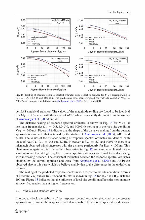
Fig. 14 Scaling of median response spectral ordinates with respect to distance for MW 6 corresponding tofosc = 0.5, 1.0, 5.0, and 100.0 Hz. The predictions have been computed for rock site condition Vs30 =760 m/s and compared with those from Ambraseys et al. (2005), AB10 and AC10

our FAS empirical equation. The values of the magnitude scaling are found to be identical(for MW > 5.0) again with the values of AC10 while consistently different from the studiesof Ambraseys et al. (2005) and AB10.

The distance scaling of response spectral ordinates is shown in Fig. 14 for MW 6, atoscillator frequencies fosc = 0.5, 1.0, 5.0, and 100.0 Hz pertinent to the rock site conditionVs30 = 760 m/s. Figure 14 indicates that the shape of the distance scaling from the currentapproach is similar to that obtained by the studies of Ambraseys et al. (2005), AB10 andAC10. The values of the distance scaling of response spectral ordinates are identical withthose of AC10 at fosc = 0.5 and 1.0 Hz. However at fosc = 5.0 and 100.0 Hz there is amismatch observed which increases with the distance particularly for RJB ≥ 100 km. Thisphenomenon again verifies the earlier observation in Fig. 12 and can be explained by thesame rationale that at high fosc the response spectral ordinates are found to be decreasingwith increasing distance. The consistent mismatch between the response spectral ordinatesobtained by the current approach and those from Ambraseys et al. (2005) and AB10 areobserved also in this case which we believe mainly due to the differences in the underlyingdatasets.

The scaling of the predicted response spectrum with respect to the site condition in termsof different Vs30 values 180, 360 and 760 m/s is shown in Fig. 15 for MW 6 at a RJB distance100 km. Figure 15 indicates that the influence of local site condition affects the motion moreat lower frequencies than at higher frequencies.

7.2 Residuals and standard deviation

In order to check the stability of the response spectral ordinates predicted by the presentapproach we examine the response spectral residuals. The response spectral residuals are

123

Bull Earthquake Eng

Fig. 15 Scaling of median response spectrum with site condition in terms of Vs30 values

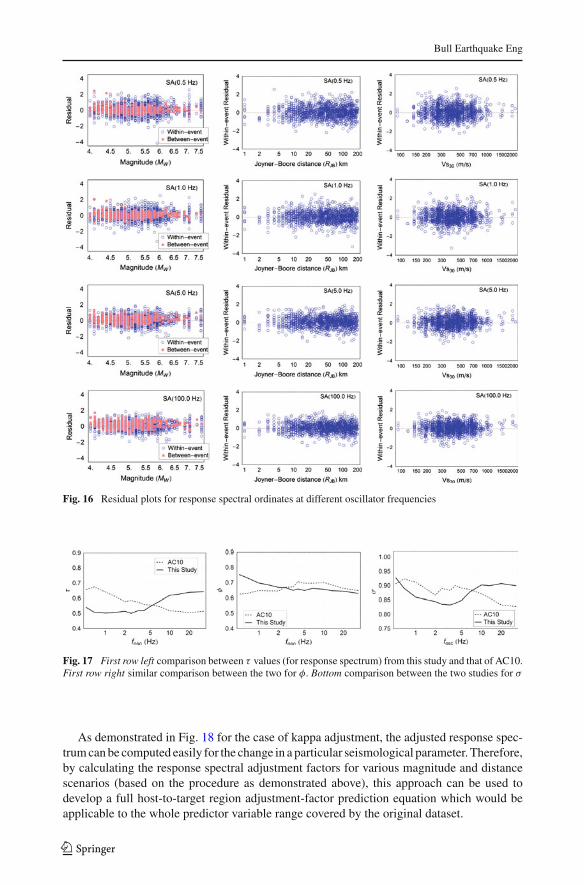
calculated as the log difference of the observed response spectral ordinates and those predictedby the combination of Fourier spectral ordinates and duration predictions. Hence it is worthnoting here that these residuals are not the direct residuals which are usually the outcome ofa regression algorithm. Again, for partitioning the residuals i.e. in between-event and within-event components the algorithm suggested by Abrahamson and Youngs (1992) was adopted.The residuals are plotted against magnitude, distance and Vs30 values at different oscillatorfrequencies fosc = 0.5, 1.0, 5.0, and 100.0 Hz in Fig. 16. Although the residuals have notbeen computed directly as an outcome of the regression procedure over the response spectralordinates, it can be observed visually that the residuals are stable with respect to magnitude,distance and Vs30. A common feature that is observed from Fig. 16 is that the between-event residuals indicate an under prediction at high frequency fosc = 100 Hz (PGA). Forfrequencies fosc = 0.5, 1.0 and 5.0 Hz the prediction is shown to be reasonable. On theother hand the within-event residuals are seen to be centered on the zero line.

The values of the standard deviations associated with the between-event and within-eventresiduals are relatively large. The variation of τ, φ and σ is depicted in Fig. 17; and com-pared with that of AC10. Figure 17 indicates that τ, φ and σ obtained from this studyare found to be reasonably comparable to those of AC10. In fact the total standard devi-ation, σ is seen to be lower than that of AC10 in the intermediate oscillator frequencyrange.

7.3 Adjustment in response spectral ordinates

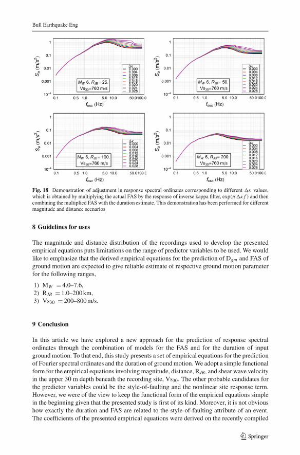
As indicated earlier that the presented approach of estimating response spectral ordinates pro-vides a physically consistent way of accommodating differences in seismological parameters.In this subsection we demonstrate the adjustment in response spectral ordinates correspond-ing to a seismological parameter, e.g. for differing values of kappa in two different regions.Although we do not estimate the kappa value of the dataset in the present study, which isanother potential application of this approach, we attempt to demonstrate the adjustment fordifferent kappa values (�κ = κ ′−κ). Here κ is the actual kappa parameter of the FAS model.We multiply the median predicted FAS by an inverse kappa filter, exp(π�κ f ) for different�κ values. Subsequently the modified FAS is combined with Dgm estimated for the samescenario to achieve the modified response spectrum. Variation of the modified response spec-tra with different values are depicted in Fig. 18 for scenarios MW = 6.0, RJB = 25, 50, 100and 200 km.

123

Bull Earthquake Eng

Fig. 16 Residual plots for response spectral ordinates at different oscillator frequencies

Fig. 17 First row left comparison between τ values (for response spectrum) from this study and that of AC10.First row right similar comparison between the two for φ. Bottom comparison between the two studies for σ

As demonstrated in Fig. 18 for the case of kappa adjustment, the adjusted response spec-trum can be computed easily for the change in a particular seismological parameter. Therefore,by calculating the response spectral adjustment factors for various magnitude and distancescenarios (based on the procedure as demonstrated above), this approach can be used todevelop a full host-to-target region adjustment-factor prediction equation which would beapplicable to the whole predictor variable range covered by the original dataset.

123

Bull Earthquake Eng

Fig. 18 Demonstration of adjustment in response spectral ordinates corresponding to different �κ values,which is obtained by multiplying the actual FAS by the response of inverse kappa filter, exp(π�κ f ) and thencombining the multiplied FAS with the duration estimate. This demonstration has been performed for differentmagnitude and distance scenarios

8 Guidelines for uses

The magnitude and distance distribution of the recordings used to develop the presentedempirical equations puts limitations on the range of predictor variables to be used. We wouldlike to emphasize that the derived empirical equations for the prediction of Dgm and FAS ofground motion are expected to give reliable estimate of respective ground motion parameterfor the following ranges,

1) MW = 4.0–7.6,2) RJB = 1.0–200 km,3) Vs30 = 200–800 m/s.

9 Conclusion

In this article we have explored a new approach for the prediction of response spectralordinates through the combination of models for the FAS and for the duration of inputground motion. To that end, this study presents a set of empirical equations for the predictionof Fourier spectral ordinates and the duration of ground motion. We adopt a simple functionalform for the empirical equations involving magnitude, distance, RJB, and shear wave velocityin the upper 30 m depth beneath the recording site, Vs30. The other probable candidates forthe predictor variables could be the style-of-faulting and the nonlinear site response term.However, we were of the view to keep the functional form of the empirical equations simplein the beginning given that the presented study is first of its kind. Moreover, it is not obvioushow exactly the duration and FAS are related to the style-of-faulting attribute of an event.The coefficients of the presented empirical equations were derived on the recently compiled

123

Bull Earthquake Eng

strong motion RESORCE-2012 database under the framework of SIGMA project. Though,the main objective of the present study is to address the issues related with the adjustmentof GMPEs in different seismological environments. Yet, the reasonable comparability of theresponse spectral ordinates with those of other GMPEs from the same region, Ambraseyset al. (2005), AB10 and AC10 indicates that the presented model for estimating responsespectral ordinates can be used as a stand-alone model. The standard deviation of between-event and within-event residuals of response spectra were found to be larger in comparisonto those of Ambraseys et al. (2005) and Akkar and Bommer (2010), while being comparableto those of Akkar and Cagnan (2010).

One point is worth mentioning here is that the presented study accounts for the adjustmentin the regional seismological attributes through the use of FAS model. However the durationestimates are also expected to vary at regional scale, but it is currently not known howexactly duration depends upon the regional seismological parameters like quality factor andkappa. These are the issues which need to be further investigated. Nevertheless, we believethat the present approach is a first step to overcome some of the technical challenges in theoriginal approach of (Campbell 2003, 2004) for adjustment issues. For example, we see itas advantageous that within the proposed framework the duration model, which enters thecalculation of adjustment factors is automatically fully consistent with the FAS since bothare constrained by the same data. The quantitative difference between the two approachescan only be exhibited by some sensitivity studies, which are topics of further investigation.

We envisage several improvements for the near future, such as exploring the consequencesof constraining the spectral scaling with magnitudes to constant stress drop models as wellas trying to empirically determine the relation between ground motion duration and the rmsduration used for calculating the rms motion (yrms) in RVT from the given dataset.

Acknowledgments Sanjay Singh Bora would like to thank Helmholtz graduate research school GeoSim(http://www.geo-x.net/geosim) for providing a scholarship. Present analysis of developing GMPEs is basedon a dataset taken from the RESORCE database which is compiled under the framework of SeIsmic GroundMotion Assessment (SIGMA) project. We also thank two anonymous reviewers for their suggestions andcomments which were helpful in improving the manuscript and bringing it to the present form.

References

Abrahamson NA, Silva WJ (1997) Empirical response spectral attenuation relation for shallow crustal earth-quakes. Seismol Res Lett 68(1):94–127. doi:10.1785/gssrl.68.1.94

Abrahamson NA, Youngs RR (1992) A stable algorithm for regression analyses using the random effectsmodel. Bull Seismol Soc Am 82(1):505–510

Ambraseys NN, Douglas J, Sarma SK, Smit PM (2005) Equations for estimation of strong ground motionsfrom shallow crustal earthquakes using data from Europe and the Middle East: horizontal peak groundacceleration and spectral acceleration. Bull Earthq Eng 3:1–53. doi:10.1007/s10518-005-0183-0

Akkar S, Bommer JJ (2006) Influence of long-period filter cut-off on elastic spectral displacements. EarthqEng Struct Dyn 35:1145–1165

Akkar S, Bommer JJ (2010) Empirical equations for the prediction of PGA, PGV, and spectral accelerationsin Europe, the Mediterranean region and the Middle East. Seismol Res Lett 81(2):195–206

Akkar S, Cagnan Z (2010) A Local ground-motion predictive model for Turkey, and its comparison withother regional and global ground-motion models. Bull Seismol Soc Am 100(6):2978–2995. doi:10.1785/0120090367

Akkar S, Kale Ö, Yenier E, Bommer JJ (2011) The high-frequency limit of usable response spectral ordinatesfrom filtered analogue and digital strong-motion accelerograms. Earthq Eng Struct Dyn 40:1387–1401

Akkar S, Sandikkaya MA, Senyurt M, Azari SA, Ay BÖ (2013) Reference database for seismic ground-motionin Europe (RESORCE). Bull Eq Eng submitted to the same issue

Arias A (1970) A measure of earthquake intensity. In: Hansen R (ed) Seismic design for nuclear power plants.MIT Press, Cambridge, pp 438–483

123

Bull Earthquake Eng

Atkinson GM, Boore DM (1995) Ground motion relations for Eastern North America. Bull Seismol Soc Am85(1):17–30

Atkinson GM, Mereu RF (1992) The shape of ground motion attenuation curves in Southeastern Canada. BullSeismol Soc Am 82(5):2014–2031

Bommer JJ, Martinez-Pereira A (1999) The effective duration of earthquake strong motion duration. J EarthqEng 3(2):127–172

Bommer JJ, Stafford PJ, Alarcon JE (2009) Empirical equations for the prediction of the significant, bracketed,and uniform duration of earthquake ground motion. Bull Seismol Soc Am 99(6):3217–3333

Boore DM (2003) Simulation of ground motion using the stochastic method. Pure Appl Geophys 160:635–676Boore DM, Bommer JJ (2005) Processing of strong-motion accelerograms: needs, options and consequences.

Soil Dyn Earthq Eng 25:93–115Boore DM, Joyner WB (1984) A note on the use of random vibration theory to predict peak amplitudes of

transient signals. Bull Seismol Soc Am 74(5):2035–2039Boore DM, Thompson EM (2012) Empirical improvements for estimating earthquake response spectra with

random-vibration theory. Bull Seismol Soc Am 102(2):761–772Brune J (1970) Tectonic stress and the spectra of seismic shear waves from earthquakes. J Geophys Res

75(26):4997–5009Campbell WK (2003) Prediction of strong ground motion using the hybrid empirical method and its use in

the development of ground-motion (attenuation) relations in Eastern North America. Bull Seismol Soc Am93(3):1012–1033

Campbell WK (2004) Erratum to Prediction of strong ground motion using the hybrid empirical method andits use in the development of ground-motion (attenuation) relations in Eastern North America. Bull SeismolSoc Am 94(6):2418

Cartwright DE, Longuet-Higgins MS (1956) The statistical distribution of the maxima of a Random function.Proc R Soc Lond Ser A Math Phys Sci 237(1209):212–232

Douglas J (2003) earthquake ground motion estimation using strong-motion records: a review of equationsfor the spectral ordinates. Earth Sci Rev 61:43–104

Douglas J (2011) Ground motion prediction equations 1964–2010. Final report BRGM/RP-59356-FRDouglas J, Boore DM (2011) High-frequency filtering of strong-motion records. Bull Earthq Eng 9:395–409Hanks TC, McGuire RK (1981) The character of high-frequency strong ground motion. Bull Seismol Soc Am

71:2071–2095Hermann RB (1985) An extension of random vibration theory estimates of strong ground motion to large

distances. Bull Seismol Soc Am 75(5):1447–1453Jaimes MA, Reinoso E, Ordaz M (2006) Comparison of methods to predict response spectra at intsrumented

sites given the magnitude and distance of an earthquake. J Earthq Eng 10(6):887–902Kempton JJ, Stewart JP (2006) Prediction equations for significant duration of earthquake ground motions

consideringsiteandnear-sourceeffects. Earthq Spectra 22(4):985–1013Liu L, Pezeshk S (1999) An improvement on the estimation of Pseudoresponse spectral velocity using RVT

method. Bull Seismol Soc Am 89(5):1384–1389McGuire R (1978) A simple model for estimating Fourier amplitude spectra of horizontal ground acceleration.

Bull Seismol Soc Am 68(3):803–822Reinoso E, Ordaz M, Sanchez-Sesma FJ (1990) A note on the fast computation of response spectra estimates.

Earthq Eng Struct Dyn 19:971–976Simons FJ, Hilst RD, Zuber MT (2003) Spatiospectral localization of isostatic coherence anisotropy in Aus-

tralia and its relation to seismic anisotropy: implications for lithospheric deformation. J Geophys Res108(B5):2250. doi:10.1029/2001JB000704

Sokolov V, Chin-hsiung L, Kuo-liang W (2000) Empirical model for estimating Fourier amplitude spectra ofground acceleration in Taiwan region. Earthq Eng Struct Dyn 29:339–357

Spudich P, Joyner WB, Lindh AG, Boore DM, Margaris BM, Fletcher JB (1999) SEA99: a revised groundmotion prediction relation for use in extensional tectonic regimes. Bull Seismol Soc Am 89(5):1156–1170

Stafford PJ (2006) Engineering seismological studies and seismic design criteria for the Buller region, Ph.DThesis. University of Canterbury, South Island, New Zealand

Stafford PJ, Berill J, Pettinga J (2006) New empirical equations for the Fourier amplitude spectrum of accel-eration and Arias intensity in New Zealand. In: Proceedings of First European conference on earthquakeengineering and seismology

Trifunac MD (1976) Preliminary empirical model for scaling Fourier amplitude spectra of strong groundacceleration in terms of earthquake magnitude, source-to-site distance, and recording site conditions. BullSeismol Soc Am 66(4):1343–1373

Vanmarcke EH, Lai SP (1980) Strong motion duration and rms amplitude of earthquake records. Bull SeismolSoc Am 70(4):1293–1307

123