Embed Size (px)
Citation preview
Note di Matematica 20, n. 1, 2000/2001, 111–157.
Four dimensional symplectic geometry over
the field with three elements and a moduli
space of Abelian surfaces
J. W. Hoffman and S. H. Weintraub∗Department of Mathematics, Louisiana State University, Baton Rouge, Louisiana 70803,[email protected], [email protected]
Received: 10 July 2000; accepted: 22 August 2000.
Abstract. We study certain combinatorial structures related to the simple group of order25920. Our viewpoint is to regard this group as G = PSp(4,F3), and so we describe theseconfigurations in terms of the symplectic geometry of the four dimensional space over the fieldwith three elements. Because of the isogeny between SO(5) and Sp(4) we can also describethese in terms of an inner product space of dimension five over that same field. The study ofthese configurations goes back to the 19th-century, and we relate our work to that of previousauthors. We also discuss a more modern connection: these configurations arise in the theory ofthe Igusa compactification of the moduli space of principally polarized Abelian surfaces witha level three structure.
Keywords: nsp-spread, double-six, orthogonal, symplectic, Siegel modular variety,Burkhardt quartic
MSC 2000 classification: primary 20G40, secondary 51E20, 05B25, 11F46
1. Introduction
Let V be a four-dimensional vector space over F3, the field with three ele-ments, equipped with the standard symplectic form
〈v, w〉 = v J tw where J =
0 0 1 00 0 0 1−1 0 0 00 −1 0 0
.
Let GL(4, F3) act on V on the left by g(v) = v.g−1. We obtain as isometrygroup of this form the symplectic group
Sp(V ) = Sp(4, F3) = g ∈ GL(4, F3) | g J tg = J∗The second author would like to thank the University of Gottingen for its hospitality while
part of this work was done.
112 J. W. Hoffman, S. H. Weintraub
We let G = PSp(V ) = PSp(4, F3) = Sp(4, F3)/ ± 1. G is the uniquesimple group of order 25920. This group was already studied in the 19th century.Camille Jordan devoted a whole chapter of his Traite des Substitutions [22]to it. He knew that this group appeared in the symplectic form as we havedescribed it above, and he also knew that it is a subgroup of index 2 inside thesymmetry group of the configuration of 27 lines on a cubic surface. Since thattime, a number of mathematicians, notably, Baker, Burkhardt, Coble, Coxeter,Dickson, Edge, Todd, have studied this group from a number of points of view.We became interested in this group in its role as the automorphism group ofA2(3)∗, the Igusa compactification of the Siegel modular variety of degree twoand level three, parametrizing principally polarized abelian surfaces with a levelthree structure [17]. A key point in our investigations was the identification ofA2(3)∗ with B, the desingularization of Burkhardt’s quartic B. See [20] for acareful and thorough study of this, relating the classical and modern viewpoints.
Various important subvarieties of this moduli space are naturally indexedby certain configurations in the 4-dimensional symplectic space V over F3. Theconfigurations of special interest here are those whose stabilizer subgroups aremaximal subgroups of G. These subgroups have index respectively 27, 36, 40, 40,45. A glance at the entry of the Atlas of finite simple groups [7] correspondingto G shows a simple description, in the language of the symplectic vector spaceV , of these maximal subgroups for the indices 40, 40, 45. Part of the purposeof this paper is to give a description, in terms of the symplectic geometry ofV , of the maximal subgroups of index 27 and 36. The key notion for this isthe concept of a spread of nonsingular pairs, or nsp-spread, and the relatedconcept of a double-six. We introduce these in section 2. of this paper. It turnsout that there are 27 nsp-spreads and 36 double-sixes, and that these are theconfigurations whose stabilizer subgroups are the subgroups of index 27 and 36respectively.
Both these concepts were discovered by the second author of this paper overa decade ago. However, the notion of an nsp-spread actually appeared in a notso well known paper by Coble [6]. In fact, lemma 1, and theorems 1 and 2 wereknown to A. B. Coble in 1908.
One of the goals of this paper is to explain some of the links between dif-ferent descriptions given by various authors of these combinatorial structures,and to relate them to the geometry of the moduli space. In section 3. of thispaper we introduce a combinatorial structure, the Tits building with scaffold-ing [19], derived from the symplectic description of G, and show how to inter-pret the geometry of our variety in terms of this structure, from three geometricdescriptions—those given by Burkhardt, Baker and ourselves.
With this in hand, we return to the study of these configurations in section 4..

Four dimensional symplectic geometry 113
Our viewpoint enables us to clarify some of Coble’s work, as well as that of L.E. Dickson [9].
In sections 5., 6. and 7. we carry out a more structural analysis of the maxi-mal subgroups of G. The main result is that they are all of the form H(F3)/±1for algebraic subgroups H ⊂ Sp(4) defined over F3. In section 6. we discussa Galois-twisted group that turns out to be the stabilizer of a double-six. Insection 7. we reinterpret these results in the language of an inner product spaceof dimension 5 over F3, relating our work to that of Edge [10], [11]. We concludewith some remarks on the Weyl group of E6 (which contains G as a subgroup ofindex 2.) Finally, we present a number of tables which have aided us in study-ing these structures. These tables may be of use to others wishing to study thisgroup and its related combinatorial structures.
In this paper we do not give an encyclopedic account of this group G. Thereare many aspects hardly touched upon – for instance, characteristic 2 descrip-tions of G, or relations to the theory of polytopes (see [8, 12]). Even from theperspective taken here, that of symplectic geometry over F4
3, we have not ana-lyzed every configuration studied previously, only those that seem most relevantto the geometry of the moduli space. In view of the importance of these con-figurations in the geometry of moduli spaces of abelian surfaces, and of theirintrinsic beauty, we hope that this work elucidates some of these structures.
One caveat about notation. It is a standard practice to denote by PG thegroup of projective transformations induced by a group G of linear transfor-mations. However, if G is now an algebraic group, and if PG denotes the al-gebraic subgroup of PGL(N) generated by G, it is not true in general thatPG(R) = PG(R). This fails in fact for Sp(2g) (see the discussion in sec-tion 7.). We will use PSp(2g) denote the algebraic group which is the quo-tient Sp(2g)/µ2. The symbol PG, with an unbold P , will denote the functorG(R)/(the scalars in G(R)).
It is a pleasure to thank James Hirschfeld for his insightful comments onan earlier version of this work, and in particular for bringing the work of Cobleand Edge to our attention. For the most complete general reference concerninggeometries over finite fields, consult his trilogy: [14, 15, 16]. To connect ourpaper with his books, note that a symplectic form is called a null polarity there.
2. Nsp-Spreads and related structures
Let V = (F3)4. We let l denote any line in V through the origin, and note
that l is specified by v ∈ V − 0, well-defined up to sign. In this case wesimply write l = v, where the ambiguity in v is understood. We thus observethat l = (V − 0) / ± 1 has cardinality 40. This set may be canonically
114 J. W. Hoffman, S. H. Weintraub
identified with a finite projective space:
l = P (V ) = P3 (F3) .
We let h denote any plane (through the origin) in V that is isotropic under 〈 , 〉.Thus 〈v, w〉 = 0 for any two v, w ∈ h. Note that h may be identified with acertain type of line in P3 (F3). Each h contains four l’s, and may be identifiedwith this set. If l1, l2 generate the plane h, we write h = l1 ∧ l2. We let δ denotea plane in V that is nonsingular under the symplectic form. So there existsv, w ∈ δ such that 〈v, w〉 = 0. As before we write δ = l1 ∧ l2 for a generatingset. δ determines its orthogonal complement δ⊥ with respect to the symplecticform, and we have V = δ⊕ δ⊥. We let ∆ be the unordered pair δ, δ⊥. We canidentify ∆ with the set of eight l’s that it contains. ∆ is called a nonsingularpair.
It is easy to check that every line l is contained in 4 isotropic planes and 9nonsingular pairs, so h has cardinality 40 · 4/4 = 40 and ∆ has cardinality40·9/8 = 45. We number the latter as ∆1, . . . , ∆45 and give these in table I. (Inthe table, we abbreviate v = (v1, v2, v3, v4) by v1 v2 v3 v4; since vi ∈ 0, 1, 2this is unambiguous.) It is straightforward to check that G acts transitively onl, h, and ∆.
Definition 1. A spread of nonsingular pairs, or nsp-spread, is a set σ =∆1, ∆2, ∆3, ∆4, ∆5 of nonsingular pairs with the property that for every lthere exists an i such that l ∈ ∆i.
Remark 1. Since there are 8 l’s in each ∆, and there are 40 l’s total,∆1, . . . , ∆5 is an nsp-spread if and only if ∆i ∩ ∆j = ∅ for i = j.
It is a nontrivial fact that nsp-spreads exist; that they do is at the heart ofour analysis.
Lemma 1. Let ∆1 and ∆2 be any two nonsingular pairs with ∆1 ∩∆2 = ∅.Then there exists a unique nsp-spread containing them: ∆1, . . . , ∆5.
Proof. It clearly suffices to prove this for a particular choice of ∆1, so let∆1 = ∆1. Then we must have
∆2 = ∆i for i ∈ 26, 27, 28, 29, 30, 37, 38, 39, 42, 43, 44, 45.
Each of these choices of i yields a unique nsp-spread, the nsp-spreads being
∆1, ∆26, ∆37, ∆44, ∆45∆1, ∆27, ∆30, ∆38, ∆42∆1, ∆28, ∆29, ∆39, ∆43
QED

Four dimensional symplectic geometry 115
Theorem 1. There are 27 nsp-spreads.Proof. Each nsp-spread contains 5 nonsingular pairs. As the proof of lemma
1 shows, each nonsingular pair is contained in 3 nsp-spreads. Since there are 45nonsingular pairs, there are 45 · 3/5 = 27 nsp-spreads. QED
We number the nsp-spreads σj , j = 1, . . . , 27, and give them in Table II.It is straightforward to check that G acts transitively on σ.Definition 2. A doublet σ1, σ2 is a disjoint pair of nsp-spreads.Definition 3. A double-six is a set consisting of two ordered collections of
six nsp-spreads
(σ1,1, σ1,2, σ1,3, σ1,4, σ1,5, σ1,6), (σ2,1, σ2,2, σ2,3, σ2,4, σ2,5, σ2,6)
such that
σi1,j1 ∩ σi2,j2 =
a single nonsingular pair if i1 = i2 and j1 = j2
∅ otherwise
In identifying double-sixes (σ1,i), (σ2,i), we are free to interchange (σ1,i) with(σ2,i) and to perform the same permutation of six objects to (σ1,i) and (σ2,i).There are six doublets in a double-six, namely the σ1,i, σ2,i for i = 1, . . . , 6.
It is a nontrivial fact that double-sixes exist.Theorem 2. There are 216 doublets. If σ1, σ2 is a doublet, then there is
a unique double-six θ = (σ1,i), (σ2,i) with σ1 = σ1,1 and σ2 = σ2,1. There are36 double-sixes.
Proof. Consider an nsp-spread σi. This nsp-spread contains 5 nonsingularpairs, each of which is contained in 3 nsp-spreads, that is, in 2 nsp-spreads otherthan σi. Thus, σi intersects 5 · 2 = 10 other nsp-spreads (as σi is the only nsp-spread containing 2 of these pairs, by lemma 1), and as there are 27 nsp-spreadsin all, σi is disjoint from 16 others. Therefore there are 27 ·16/2 = 216 doublets.
To show that double-sixes exist, we exhibit one. The doublet σ22, σ26 iscontained in the unique double-six
(σ22, σ8, σ1, σ6, σ27, σ14), (σ26, σ3, σ5, σ7, σ13, σ24).
It is straightforward to check that G acts transitively on doublets, so eachdoublet is contained in a unique double-six. Since each double-six contains 6doublets, there are 216/6 = 36 double-sixes. QED
We list the doublets in Table III, grouped into double-sixes. Note that Gacts transitively on the double-sixes.
The doublets and double-sixes can be understood in terms of the structureof the group G.

116 J. W. Hoffman, S. H. Weintraub
Proposition 1. Let F ⊂ G be a Sylow 5-subgroup, and consider the actionof F ∼= Z/5 on Σ = σ1, . . . , σ27. There are exactly 2 fixed points for thisaction: σ1, σ2, and these form a doublet. Of the other 5 orbits of F on Σ,each of which consists of 5 nsp-spreads, there are 3 orbits whose nsp-spreads arepairwise disjoint. Denote these by ai, bi, and ci, i = 1, . . . , 5. Then, afterproper renumbering, we have for all i = 1, . . . , 5,
#(σ1 ∩ ai) = 0 #(σ2 ∩ ai) = 1#(σ1 ∩ bi) = 1 #(σ2 ∩ bi) = 0#(σ1 ∩ ci) = 1 #(σ2 ∩ ci) = 1
so that(σ1, a1, . . . , a5), (σ2, b1, . . . , b5)
forms a double-six.
Proof. Since all 5-Sylow subgroups are conjugate, and cyclic, it will sufficeto examine the action of a single element g of order 5. Choose
g =
0 0 −1 −11 −1 0 −11 0 0 0−1 1 0 0
Then g fixes σ22 and σ26, and the sets ai and bi are given by
σ8, σ1, σ6, σ27, σ14 and σ3, σ5, σ7, σ13, σ24
respectively. QED
Remark 2. Since each double-six contains 12 nsp-spreads, each nsp-spreadis contained in 36 · 12/27 = 16 double-sixes.
Remark 3. The nsp-spreads in each “half” of a double-six contain the samecollection of nonsingular pairs, so of the 45 nonsingular pairs, 30 are containedwith multiplicity 2 in the nsp-spreads forming a double - six, while the other 15are not contained at all in these nsp-spreads.
Our analysis enables us to easily identify the structure of some of the stabi-lizers.
Lemma 2. The subgroup of G stabilizing a double-six is isomorphic to S6,the symmetric group on 6 elements. The isomorphism is given by the action ofthe stabilizer on the doublets in a double-six.

Four dimensional symplectic geometry 117
Proof. Let H be the stabilizer of a double-six. Since G acts transitivelyon the 36 double-sixes, H has order 25920/36 = 720. H obviously acts on the 6doublets contained in a double-six that it fixes, so we obtain a homomorphismϕ : H → S6. Since G acts transitively on the doublets, we see that H actstransitively on the 6 doublets in a double-six fixed by H. This is because eachdoublet is contained in a unique double-six. Hence Im(ϕ) is a transitive sub-group. We will show that Im(ϕ) = S6 by showing that it contains a 5-cycle anda transposition, [27], and this shows that ϕ is an isomorphism.
Consider the element g of proposition 1. The proof of proposition 1 showsthat ϕ(g) is a 5-cycle. Here we are thinking of H as the stabilizer of the double-six number 11 of table III.
Now consider the element of G:
t =
0 0 −1 00 0 0 −11 0 0 00 1 0 0
Calculation shows that ϕ(t) is a transposition, this time regarding H as thestabilizer of the double-six number 33. QED
Lemma 3. The subgroup of G stabilizing an nsp-spread is isomorphic to anextension of the alternating group A5 by (Z/2)4.
Proof. Let K = K(σ) be the stabilizer of the nsp-spread
σ = ∆1, ∆2, ∆3, ∆4, ∆5.
We claim that there is an exact sequence
1 −→ (Z/2)4 −→ K −→ A5 −→ 1.
We prove this by constructing homomorphisms
π : K → S5 and ρ : Ker(π) → (Z/2)5 .
with Image(π) = A5 and Image(ρ) ∼= (Z/2)4. Since K has order 25920/27 =960 = 16 · 60, this proves the claim.
Each element of K induces a permutation of the set ∆1, ∆2, ∆3, ∆4, ∆5and this gives us π. Each ∆i is a pair δ′i, δ′′i . For k ∈ K leaving ∆i invariant,we set εi(k) = +1 (resp. −1) if k fixes both δ′i and δ′′i (resp. k transposes δ′iand δ′′i ). For each k ∈ Ker(π), set ρ(k) = (ε1(k), . . . , ε5(k)). Clearly ρ is ahomomorphism.

118 J. W. Hoffman, S. H. Weintraub
We claim that Image(π) = A5 ⊂ S5 and Image(ρ) = E ⊂ (Z/2)5 where
E = (ε1, . . . , ε5) |∏
εi = 1.
Consider the element t of lemma 2. Calculation shows that t is in the stabi-lizer of σ1, the first nsp-spread of table II, and indeed, that t leaves each nonsin-gular pair in this nsp-spread invariant, so t ∈ Ker(π), π : K(σ1) → S5. Furthercalculation shows that ρ(t) = (1,−1,−1,−1,−1). Also, calculation shows thatthe element g of proposition 1, which leaves nsp-spread σ22 of table II invariant,acts as a 5-cycle on the nonsingular pairs contained therein. Since all stabilizersare conjugate, there is an element g′ ∈ K(σ1) such that π(g′) is a 5-cycle. Thenconjugating t by powers of g′ gives elements ti ∈ Ker(π) with ρ(ti) = (ε1, . . . , ε5)where εj = 1 if j = i and εj = −1 if j = i. These elements generate the sub-group E so Im(ρ) ⊃ E. Therefore, 16 divides the order of Im(ρ) and hence theorder of Ker(π).
Calculation shows that t leaves the nsp-spread σ2 invariant, but it does notfix each of the nonsingular pairs that it contains. In fact π(t) is a product oftwo disjoint transpositions, where this time π : K(σ2) → S5.
Finally, calculation shows that the element of G of order 3:
s =
1 0 1 00 1 0 00 0 1 00 0 0 1
leaves σ1 invariant, and π(s) is a 3-cycle, π : K(σ1) → S5.We have seen that 16 divides the order of Ker(π) and that Im(π) has elements
of order 2, 3, 5. Thus 30 divides the order of Im(π). Since K has order 960, eitherKer(π) has order 16 and Im(π) has order 60 or Ker(π) has order 32 and Im(π)has order 30. But the latter case is impossible since S5 has no subgroups oforder 30. Thus we are in the former case, with Im(ρ) isomorphic with (Z/2)4,and Im(π) being A5, the unique subgroup of S5 of order 60. QED
Theorem 3. There are G-equivariant identifications
nsp-spreads ↔ lines on the cubic surfacedouble-sixes ↔ double-sixes of lines on the cubic surface
nonsingular pairs ↔ tritangent planes to the cubic surface
Proof. The cardinalities of these sets match up, being 27, 36, and 45 re-spectively, and in all cases G acts transitively on the set. Thus the stabilizer ofeach of these is a subgroup of index 27, 36, and 45 (= order 960, 720, and 576)
Four dimensional symplectic geometry 119
respectively. However, Dickson [9] has shown that there is a unique conjugacyclass of subgroups of G of each of these orders.
For a constructive proof, note that if the third identification holds, the firsttwo follow (as an nsp-spread is determined by the pairs it contains, and a lineon the cubic by the 5 tritangent planes on which it lies).
But now note that the stabilizer of the non singular pair
(1000) ∧ (0010), (0100) ∧ (0001)
is the image in G of the subgroup
a1 0 b1 00 a2 0 b2c1 0 d1 00 c2 0 d2
⋃
0 a1 0 b1a2 0 b2 00 c1 0 d1
c2 0 d2 0
of Sp(4, F3), where
(ai bici di
)∈ SL(2, F3) for i = 1, 2
and this is exactly the subgroup stabilizing a tritangent plane [7, p. 26]. (Notethat [7] works projectively, so that what we describe as a line (resp. isotropicplane) is described there as a point (resp. isotropic line).) QED
Remark 4. Given theorem 3, we observe that lemmas 2 and 3 verify thestructures of the stabilizers given in [7].
In addition to considering the symplectic group Sp(V ), we may also considerthe group of symplectic similitudes
GSp(V ) = GSp(4, F3) = g ∈ GL(4, F3) | gJ tg = λJ, λ ∈ F∗3
Let G = GSp(4, F3)/ ± 1. Then G is a group of order 51480 having G as asubgroup of index two. A representative of the nontrivial coset is the elementof order two
g0 =
1 0 0 00 1 0 00 0 −1 00 0 0 −1
.
Note that G acts on all the objects that we have considered here (isotropic linesand planes, nonsingular pairs, nsp-spreads and double-sixes).
120 J. W. Hoffman, S. H. Weintraub
Proposition 2.
1. The element g0 leaves seven nonsingular pairs invariant and permutes theother 38 in pairs.
2. The element g0 leaves three nsp-spreads invariant and permutes the other24 in pairs.
3. The subgroup of G stabilizing a double-six is isomorphic to S6 × S2.
4. The subgroup of G stabilizing an nsp-spread is isomorphic to an extensionof S5 by (Z/2)4.
Proof. a) Direct calculation. On non-singular pairs, g0 acts as the permu-tation
(4 5)(6 8)(7 9)(10 13)(11 14)(12 15)(17 18)(20 21)(22 23)(24 25)(27 28)(29 30)(31 40)(32 34)(33 35)(36 41)(38 39)(42 43)(44 45).
b) Direct calculation. On nsp-spreads, g0 acts as the permutation
(2 3)(5 6)(8 9)(10 13)(11 14)(12 15)(16 22)(17 23)(18 24)(19 25)(20 26)(21 27).
c) Let H be the stabilizer in G of a double-six, and H the stabilizer in G ofa double-six. Let ϕ = (ϕ, ϕ′) : H → S6 × S2, where ϕ is the map of lemma 2and ϕ′(h) is the action of h on the two “halves” of a double-six (either leavingthem invariant or interchanging them). It is easy to check, from the proof oflemma 2, that the image of H under ϕ is the subgroup of S6 × S2 consisting ofpermutations (α, α′) with sgn(α) = sgn(α′).
The element g0 stabilizes the double-six θ20 and direct calculation showsthat ϕ(g0) is a product of two transpositions, while ϕ′(g0) is a transposition, soϕ(g0) /∈ Im(H) and hence ϕ : H → S6 × S2 is an isomorphism.
d) Let K be the stabilizer in G of an nsp-spread and K the stabilizer in Gof an nsp-spread. Let π be the map of lemma 3. The element g0 stabilizes thensp-spread σ1 and direct calculation shows that π(g0) is a transposition, hencenot an element of A5 = Im(K), so π(K) = S5, and the result follows as in theproof of lemma 3. QED
We conclude this section by considering the notion of an nsp-spread in gen-eral.
Definition 4. Let V be a 2n-dimensional vector space over a field F, neven, equipped with a nonsingular symplectic form 〈 , 〉. A nonsingular pair∆ = δ1, δ2 is the image in P(V ) of a pair of n-dimensional subspaces δ1, δ2,
Four dimensional symplectic geometry 121
each of which is nonsingular under the restriction of 〈 , 〉, and such thatV = δ1 ⊕ δ2. An nsp-spread is a set
σ = ∆ii∈I
of pairwise disjoint nonsingular pairs such that⋃i∈I
∆i = P(V )
where ∆i is identified with the set of projective lines that it contains.We can show that nsp-spreads exist in considerable generality. In particular,
they exist for any even n and F any finite field of odd characteristic, or anynumber field. See [18].
3. The Tits building with scaffolding
We briefly recall the definition of the Tits building with scaffolding T (V ) ofthe symplectic vector space V [19, 17]. (Our description here is simplified a bitbecause the units of Z/3 are just ±1.)
T (V ) is a graph with vertices
l of cardinality 40h of cardinality 40∆ of cardinality 45
and edges
l, h if l ⊂ h, of cardinality 160l, ∆ if l ⊂ ∆, of cardinality 360
(The full subcomplex l, h, l, h is the usual Tits building T (V ).)The action of G on V/± 1 clearly induces an action on T (V ).We have the following description of A2(3)∗, the Siegel modular variety of
degree two and level three [17]: The variety A2(3)∗ is the Igusa compactificationof A2(3) = Γ(3)\S2, where S2 is the degree two Siegel space, and Γ(3) is theprincipal congruence subgroup of level 3 in Γ(1) = PSp(4, Z). The quotientΓ(1)/Γ(3) = PSp(4, F3) = G acts on A2(3) and this action extends to thecompactification A2(3)∗. The “boundary” of A2(3)∗ is
A2(3)∗ −A2(3) =⋃l
D(l)

122 J. W. Hoffman, S. H. Weintraub
where each D(l) is Shioda’s elliptic modular surface of level 3. We call such aD(l) a corank 1 boundary component.
Figure 1. Corank 1 boundary component D(l)
Each of these is a family of genus 1 curves, parameterized by a copy M(l) ∼=P1 of the modular curve of level 3. Over four points of M(l), the “cusps”,the general fiber degenerates into a triangle of P1’s. Hence, each D(l) has fourtriangles of rational lines on it. There are also nine cross-sections of the fibrationD(l) →M(l), not pictured in figure 1.
The D(l) are not pairwise disjoint; if two of them intersect, the intersectionis one of the P1’s in the 4 distinguished triangles. The union of all these inter-sections form 40 connected components C(h), each of which is a “tetrahedron”of P1’s. Moreover, D(l1) intersects D(l2) if and only if h = l1 ∧ l2. In this case
Figure 2. Corank 2 boundary component C(h)

Four dimensional symplectic geometry 123
we say that l1, l2 is an incident pair.
A2(3)∗ contains 45 Humbert surfacesH(∆) (of discriminant 1), each of whichis isomorphic with M(l) ×M(l) ∼= P1 × P1. Each of these has 8 distinguishedrational lines, namely the cusp ×M(l) and the M(l) × cusp.
These are mutually disjoint, and H(∆) ∩D(l) if nonempty, is equal one ofthe 9 sections of the elliptic modular surface D(l), and it is also equal to one ofthe 8 distinguished rational lines on H(∆). The intersection is nonempty if andonly if l is in ∆.
A2(3)∗ is identified with B, and blowing down each of the 45 Humbertsurfaces yields a quartic projective threefold with 45 ordinary double points(Burkhardt’s quartic). We refer the reader to [20] for a further discussion of B.
Figure 3. Humbert surface H(∆)
We now present our dictionary, showing how to translate between Burk-hardt’s language [3, 4, 5], Baker’s language [1], and ours [17]: (We have labeledeach object with its cardinality.)

124 J. W. Hoffman, S. H. Weintraub
Dictionary
(40) Vertex l of T (V ) : Burkhardt–Hauptebene: Baker–Jacobi plane: A2(3)∗-corank 1 boundary
component D(l)
(40) Vertex h of T (V ) : Burkhardt–Hauptraum erster Art: Baker–Steiner tetrahedron: A2(3)∗-corank 2 boundary
component C(h)
(45) Vertex ∆ of T (V ) : Burkhardt–Hauptraum zweiter Art: Baker-node: A2(3)∗-Humbert surface H(∆)
(160) Edge (l, h) of T (V ) : A2(3)∗-exceptional fiber in D(l)(or “face” of a tetrahedron in C(h))
(360) Edge (l, ∆) of T (V ) : A2(3)∗-section of D(l)
(240) Incident pair l1, l2 of T (V ) : Burkhardt–Hauptgerade: Baker-κ line
: A2(3)∗-exceptional P1
= D(l1) ∩D(l2) ⊂ C(l1 ∧ l2)
(27) Nsp-spread ∆1, . . . ,∆5 of T (V ) : Burkhardt-Pentatope zweiter Art: Baker–Jordan pentahedron: A2(3)∗-set of 5 Humbert surfacesH(∆1), . . . , H(∆5)intersecting every D(l)
Four dimensional symplectic geometry 125
4. Coble and Dickson
We now turn to the work of Coble [6] and Dickson [9]. V is therefore a fourdimensional symplectic vector space. For the rest of this section we will workprojectively, so that l, h, and δ become an (isotropic) point, an isotropic lineand a nonsingular line, and δ⊥ the complementary line to δ. We still call ∆, σ,and θ a nonsingular pair, nsp-spread, and double-six.
Although Coble did not refer to Dickson in his work, we shall first investigateDickson’s work and then use our results to explain Coble’s. We begin with somegeneral notation and language.
Definition 5. Let a group A operate on a set X. For x ∈ X, let P (x)denote the stabilizer subgroup of x,
P (x) = a ∈ A | a(x) = x.
If A acts transitively on X then the index of P (x) in A is the cardinality of X.
Lemma 4. Let a group A operate transitively on a set X.
1. For any x1, x2 ∈ X, P (x1) and P (x2) are mutually conjugate in A.
2. The following are equivalent:
i. For any x1 = x2 ∈ X, P (x1) = P (x2).
ii. For any x ∈ X, B = P (x) satisfies B = N(B), i.e., B is its ownnormalizer in A.
3. Define an equivalence relation ∼ on X by x1 ∼ x2 if P (x1) = P (x2).Then every equivalence class has [N(B) : B] elements, where B = P (x).
Definition 6. If B is a subgroup of A such that N(B) = B, then we saythat B is self-conjugate (in A). (Here we follow Dickson’s language.)
Definition 7. Let X be a set.
1. A subset of m elements of X is an m-ad. For m = 2 or 3, an m-ad is aduad or a triad, respectively.
2. If X has n elements, and n is a multiple of m, an unordered partition ofX into n/m m-ads is an m-adic syntheme. (This language was introducedby Sylvester in 1844.)
Theorem 4. (Dickson 1904 [9]) G = PSp(4,F3) has exactly 114 conjugacyclasses of proper subgroups, of which 18 are self-conjugate.

126 J. W. Hoffman, S. H. Weintraub
Dickson’s approach was purely algebraic. Our aim here is to understandthese 18 self-conjugate subgroups by using the geometry of the vector space V ,or more precisely, by using configurations arising from objects we have alreadyconsidered. We follow Dickson’s notation for these subgroups. In particular, thesubscript attached to a subgroup denotes its order.
Theorem 5. The 18 self-conjugate subgroups of G arise as follows:
1. G20, of index 1296, is the normalizer of a 5 - Sylow subgroup.
2. G∗24, of index 1080, is the stabilizer of a pair (h, σ).
3. K∗36, of index 720, is the stabilizer of a pair (h, ∆) with h ∩ ∆ = ∅.
4. G48, of index 540, is the stabilizer of a duadic syntheme of doublets in adouble-six θ.
5. G72, of index 360, is the stabilizer of a pair (l, ∆) with l ⊂ ∆.
6. G∗∗72, of index 360, is the stabilizer of a triadic syntheme of doublets in a
double-six θ.
7. H96, of index 270, is the stabilizer of a duad of nonsingular pairs in annsp-spread σ.
8. G120, of index 216, is the stabilizer of a doublet.
9. G′120, of index 216, is the image of G120 under the outer automorphism of
G720.
10. G160, of index 162, arises as follows:
1 −→ (Z/2)4 −→ G960π−→ A5 −→ 1
||⋃ ⋃
1 −→ (Z/2)4 −→ G160 −→ N10 −→ 1
where N10 is the normalizer (in A5) of a 5-Sylow subgroup.
11. G162, of index 160, is the stabilizer of a pair (l, h) with l ⊂ h.
12. G192, of index 135, is the stabilizer of a pair (∆, σ) with ∆ ∈ σ.
13. H216, of index 120, is the stabilizer of a duadic syntheme of l’s in an h.
14. G576, of index 45, is the stabilizer of a nonsingular pair ∆.
15. G648, of index 40, is the stabilizer of a point l.

Four dimensional symplectic geometry 127
16. H648, of index 40, is the stabilizer of an isotropic line h.
17. G720, of index 36, is the stabilizer of a double-six θ.
18. G960, of index 27, is the stabilizer of an nsp-spread σ.
Remark 5. a) Since, by lemma 1, any two disjoint nonsingular pairsare contained in a unique nsp-spread, H96 can also be described as thestabilizer of a duad of disjoint nonsingular pairs.
b) The symmetric group of order 6 has a unique (up to inner automorphisms)outer automorphism, as observed by Todd [26]. By lemma 2, the subgroupG720 is isomorphic to S6, and G120 is a subgroup of G720, so applying thisautomorphism takes G120 to G′
120.
c) The top line in the construction of G160 is the exact sequence in the proofof lemma 3. Also, N10 = π (G10) where G10 is the unique (up to conjugacy)subgroup of G of order 10. (Note that G10 = G20 ∩ π−1 (A5)).
Proof. The difficult part of the theorem is discovering the configurationsthat are stabilized. Once this is done, verifying that the stabilizers are as claimedis a (more or less) routine calculation, and so we omit it. QED
Remark 6. In comparing the entries in the “Dictionary” of section 3.with the configurations of the above theorem, one is missing, that of an in-cident pair l1, l2. But, l1 and l2 are incident if and only if they are bothcontained in some isotropic line h. Now h contains 4 l’s, say l1, l2, l3, l4.Thus, P (l1, l2) ⊂ P (h), and then if l1, l2 is stabilized, so is l3, l4. ThusP (l1, l2) = P (l3, l4), and this subgroup is not self-conjugate. However, it isof index two in P (l1, l2, l3, l4) = H216, of index 120, which does appearin the theorem.
Some self-conjugate subgroups can be realized in more than one way as thestabilizer of a configuration. Perhaps the most interesting of these is G48 ofindex 540.
Proposition 3. a) Given a pair (h1, ∆) with h1∩∆ = ∅, then there is aunique h2 = h1 with h2 ∩∆ = ∅ and P (h1, ∆) = P (h2, ∆). Furthermore,h1 and h2 are disjoint.
b) Given a duad (h1, h2) of disjoint isotropic lines, there is a unique nonsin-gular pair ∆ with P (h1, ∆) = P (h2, ∆). Furthermore, h1 ∩ ∆ = ∅ andh2 ∩ ∆ = ∅.
c) In this situation, P (hi, ∆) is a normal subgroup of index 2 in
P (h1, h2, ∆) = P (h1, h2)
128 J. W. Hoffman, S. H. Weintraub
Also, P (h1, h2, ∆) = G48.Proof. First let us see that the cardinality of each of these sets is 540. In
a) there are 45 ∆’s, and each is disjoint from 24 h’s, so when the h’s are pairedwe get 540 = 45 · 24/2 sets h1, h2, ∆. In b), there are 40 h’s, and eachis disjoint from 27 other h’s, and this pair determines a unique ∆, so we get540 = (40 · 27)/2) · 1 sets h1, h2, ∆. In c), there are 36 double-sixes, and aset of 6 objects has
13!
(62
)(42
)(22
)= 15 duadic synthemes,
so we get 540 = 36 · 15 duadic synthemes of doublets in a double-six.Thus to construct a bijective correspondence between these objects we need
only construct an injective mapping between them.Also, given a duad h1, h2 of disjoint h’s, there is an element of G which
interchanges h1 and h2. Assuming b), the uniqueness of ∆ implies that anyelement of G which stabilizes h1, h2 must also stabilize ∆, verifying all butthe last claim in c).
First we show how to pass from a duadic syntheme of doublets in a double-sixto a set h1, h2, ∆. Consider a duadic syntheme (ij)(kl)(mn) of doublets ina fixed double-six θ. Then the doublets i and j, regarded as sets of nonsingularpairs, intersect in two nonsingular pairs ∆1
ij and ∆2ij , and similarly for the
doublets k and l and the doublets m and n. The nonsingular pairs ∆1ij and ∆2
ij
are disjoint and so determine a unique nsp-spread σij , and similarly for k and land m and n. Then, as sets of nonsingular pairs,
σij ∩ σkl ∩ σmn = ∆
for a unique ∆. (Otherwise σij , σkl, σmn are pairwise disjoint.) As sets of l’s,
∆1ij ∪ ∆2
ij ∪ . . . ∪ ∆2mn = 24 l’s.
∆ contains 8 l’s, disjoint from the above 24. Together these give 32 of the 40l’s. The remaining 8 can be grouped into a unique way into h1 and h2.
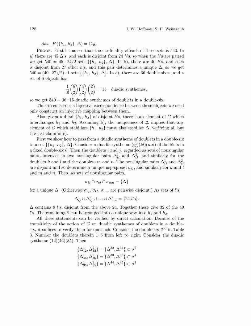
All these statements can be verified by direct calculation. Because of thetransitivity of the action of G on duadic synthemes of doublets in a double-six, it suffices to verify them for one such. Consider the double-six θ36 in Table3. Number the doublets therein 1–6 from left to right. Consider the duadicsyntheme (12)(46)(35). Then
∆112,∆
212 = ∆32,∆34 ⊂ σ7
∆146,∆
246 = ∆33,∆35 ⊂ σ4
∆135,∆
235 = ∆44,∆45 ⊂ σ1

Four dimensional symplectic geometry 129
and σ7 ∩ σ4 ∩ σ1 = ∆26 so ∆ = ∆26. The remaining 8 l’s are
(0001), (0010), (0011), (0012), (0100), (1000), (1100), (1200)
which can be grouped into
h1 = (0001), (0010), (0011), (0012) and h2 = (0100), (1000), (1100), (1200).
Next we show how to pass from (h1, ∆) to (h2, ∆) and thus to (h1, h2). Let∆ = δ, δ⊥ and consider
αl + βl′ | l ∈ δ, l′ ∈ δ⊥, α/β = ±1
This set consists of 32 l’s, all those not in ∆. Then h2 is defined by the conditionαl+βl′ ⊂ h1 ⇔ αl−βl′ ⊂ h2. Again this can be checked by direct computationin the above example, and by transitivity it suffices to consider a single example.
Thus we have correspondences between the various objects in the proposi-tion, and it is routine to verify that they are injective, completing the proof.
QED
Definition 8. If h1, h2 and ∆ are as in the above proposition, i.e., P (h1,∆)= P (h2,∆), then h1, h2 and ∆ are called related.
While this result deals with the case h ∩ ∆ = ∅, in connection with parts2 and 3 of theorem 5, and for our work below, we wish to expand on the caseh ∩ ∆ = ∅.
Proposition 4. 1. Suppose that h ∩ ∆ = ∅. Then, after proper number-ing, h ∩ ∆ = l1, l2 where h = l1, l2, l3, l4, ∆ = δ, δ⊥ and l1 ∈ δ,l2 ∈ δ⊥.
2. For any fixed duad l1, l2 ⊂ h, there are exactly three ∆’s with h ∩ ∆ =l1, l2.
3. Fix h and σ arbitrarily. Then there are exactly two (necessarily disjoint)nonsingular pairs ∆1, ∆2 ⊂ σ with ∆i ∩ h = ∅. In that case, after properrenumbering ∆1∩h = l1, l2, and ∆2∩h = l3, l4 with h = l1, l2, l3, l4.
In the situation of c) we call the duads l1, l2 and l3, l4 complementary.Proof. Routine. QED
Now we come to the work of Coble [6]. Let us begin by comparing our lan-guage and notation with his. We denote points by l; Coble denoted them P . Wehave isotropic lines h; Coble called these complex lines C. We have nonsingu-lar lines δ, which determine their orthogonal complements δ⊥ and nonsingularpairs ∆ = δ, δ⊥; Coble had non-complex lines N which determine conjugate

130 J. W. Hoffman, S. H. Weintraub
non-complex lines N ′ and skew pairs NN ′. An isotropic line h with ∆∩h = ∅ orin Coble’s language a complex line C with C ∩NN ′ = ∅ he called a transversalof NN ′. We have spreads of nonsingular pairs σ; Coble had sets of five skewpairs of conjugate lines F . Finally, we have double-sixes θ, and Coble also calledthese double-sixes.
First we observe that Coble knew proposition 4 and used it to count nsp-spreads (in our language) as follows: Since an nsp-spread contains every l once,it intersects every h twice. Fix an h = l1, . . . , l4. Then there are three waysto choose a duadic syntheme of l’s in h. Fix one, l1, l2, l3, l4. Then thereare three ways to choose ∆1 with ∆1 ∩ h = l1, l2 and three ways to choose∆2 with ∆2 ∩ h = l3, l4. The nonsingular pairs ∆1 and ∆2 are necessarilydisjoint and so extend to a unique nsp-spread σ. Thus there are 3 · 3 · 3 = 27nsp-spreads.
To proceed further, let us recall the tetrahedron C(h) constructed in thebeginning of section 3.. The four faces of the tetrahedron correspond to the fourl’s in an h. The six edges correspond to the six duads li, lj of l’s in an h(being the intersection of the faces corresponding to li and lj). In a tetrahedroneach edge has a unique opposite edge, i.e., the edge to which it is not adjacent.The edge corresponding to the duad l1, l2 has as its opposite edge the edgecorresponding to the complementary duad l3, l4.
Now fix h = l1, . . . , l4. For any duad li, lj of l’s in h, there are threenonsingular pairs ∆1, ∆2, ∆3 with ∆k ∩ h = li, lj, k = 1, 2, 3. Coble calls∆1, ∆2, ∆3 a triad. If li′ , lj′ is the complementary duad to li, lj, thenthere are three other nonsingular pairs ∆4, ∆5, ∆6 with ∆k ∩ h = li′ , lj′,k = 4, 5, 6. Coble calls ∆4, ∆5, ∆6 the conjugate triad to ∆1, ∆2, ∆3. Thuseach of the three duadic synthemes of l’s in an h determines a pair of conjugatetriads. Coble calls the union of these three pairs of conjugate triads a triadcomplex. We see that the triad complexes are in bijective correspondence withthe isotropic lines, hence there are 40 of them. (Coble constructed them in aslightly different way.)
We have observed earlier (as did Coble) that any two disjoint nonsingularpairs ∆1, ∆2 are contained in a unique nsp-spread σ = ∆1, ∆2, ∆3, ∆4, ∆5,and so determine ∆3, ∆4, ∆5. We shall call ∆3, ∆4, ∆5 the complementarytriad to the duad ∆1, ∆2.
We now consider certain polygons, by which we mean configurations ofpoints and lines. We must distinguish between two kinds, polygons in P3 =P(V ), where point and lines have their usual meaning, and “abstract” poly-gons, where we have notions of point, line, and incidence (but these are notsubsets of P3). We shall be considering two general types, quadrilaterals, whichmay be in P3 or abstract, and complex hexagons, which are abstract.These poly-
Four dimensional symplectic geometry 131
gons were defined by Coble. Our point here is to clarify their meaning. Again, weshall (mostly) omit proofs of these results; once the facts have been discoveredtheir verification is routine. We follow Coble’s notation for these polygons.
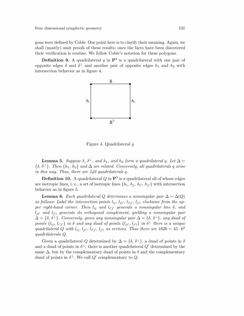
Definition 9. A quadrilateral q in P3 is a quadrilateral with one pair ofopposite edges δ and δ⊥ and another pair of opposite edges h1 and h2 withintersection behavior as in figure 4.
qh
δ
δ
1 h2
Figure 4. Quadrilateral q
Lemma 5. Suppose δ, δ⊥, and h1, and h2 form a quadrilateral q. Let ∆ =δ, δ⊥. Then h1, h2 and ∆ are related. Conversely, all quadrilaterals q arisein this way. Thus, there are 540 quadrilaterals q.
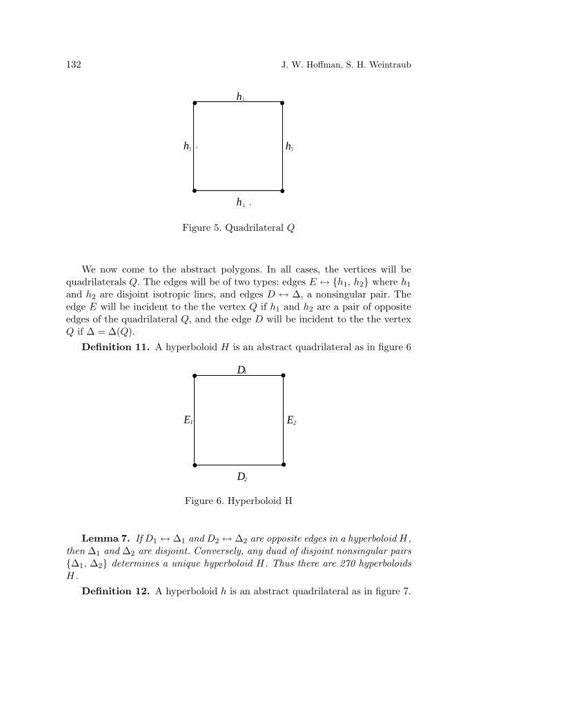
Definition 10. A quadrilateral Q in P3 is a quadrilateral all of whose edgesare isotropic lines, i. e., a set of isotropic lines hi, hj , hi′ , hj′ with intersectionbehavior as in figure 5.
Lemma 6. Each quadrilateral Q determines a nonsingular pair ∆ = ∆(Q)as follows: Label the intersection points lij , lji′ , li′j′ , lj′i clockwise from the up-per right-hand corner. Then lij and li′j′ generate a nonsingular line δ, andlji′ and lj′i generate its orthogonal complement, yielding a nonsingular pair∆ = δ, δ⊥. Conversely, given any nonsingular pair ∆ = δ, δ⊥, any duad ofpoints lij , li′j′ in δ and any duad of points lji′ , lj′i in δ⊥ there is a uniquequadrilateral Q with lij , lji′ , li′j′ , lj′i as vertices. Thus there are 1620 = 45 · 62
quadrilaterals Q.
Given a quadrilateral Q determined by ∆ = δ, δ⊥, a duad of points in δand a duad of points in δ⊥, there is another quadrilateral Q′ determined by thesame ∆, but by the complementary duad of points in δ and the complementaryduad of points in δ⊥. We call Q′ complementary to Q.
132 J. W. Hoffman, S. H. Weintraub
Qh
h
h
h j ' j
i '
i
Figure 5. Quadrilateral Q
We now come to the abstract polygons. In all cases, the vertices will bequadrilaterals Q. The edges will be of two types: edges E ↔ h1, h2 where h1
and h2 are disjoint isotropic lines, and edges D ↔ ∆, a nonsingular pair. Theedge E will be incident to the the vertex Q if h1 and h2 are a pair of oppositeedges of the quadrilateral Q, and the edge D will be incident to the the vertexQ if ∆ = ∆(Q).
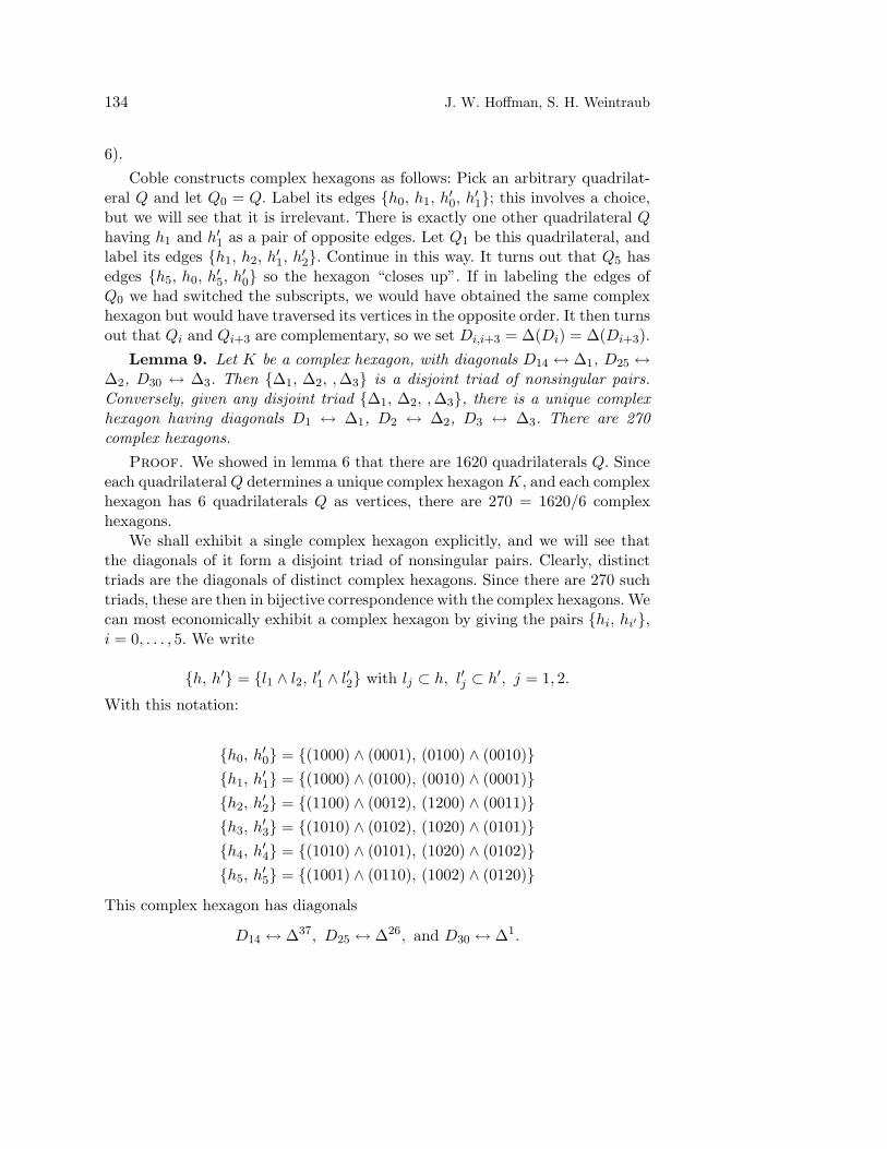
Definition 11. A hyperboloid H is an abstract quadrilateral as in figure 6
HE
D
D
E1 2
2
1
Figure 6. Hyperboloid H
Lemma 7. If D1 ↔ ∆1 and D2 ↔ ∆2 are opposite edges in a hyperboloid H,then ∆1 and ∆2 are disjoint. Conversely, any duad of disjoint nonsingular pairs∆1, ∆2 determines a unique hyperboloid H. Thus there are 270 hyperboloidsH.
Definition 12. A hyperboloid h is an abstract quadrilateral as in figure 7.

Four dimensional symplectic geometry 133
hE
D
E
E1 2
Figure 7. Hyperboloid h
This is the one place where Coble’s notation conflicts with ours. The meaningof h should be clear in context.
Lemma 8. If D ↔ ∆ and E ↔ h1, h2 are opposite edges in a hyperboloidh, then h1, h2 and ∆ are related. Conversely, if h1, h2 and ∆ are related,they determine a unique hyperboloid h. Thus there are 540 hyperboloids h.
Figure 8. Complex hexagon
We now come to the most elaborate of Coble’s configurations, the complexhexagon.
Definition 13. A complex hexagon K is an abstract configuration as infigure 8, where the six edges are lines of type E and the three diagonals arelines of type D. We let Qi, i = 0, . . . , 5 be the vertices, Ei,i+1 the edge joiningQi and Qi+1, and Di,i+3 the diagonal joining Qi and Qi+3 (all subscripts modulo
134 J. W. Hoffman, S. H. Weintraub
6).Coble constructs complex hexagons as follows: Pick an arbitrary quadrilat-
eral Q and let Q0 = Q. Label its edges h0, h1, h′0, h
′1; this involves a choice,
but we will see that it is irrelevant. There is exactly one other quadrilateral Qhaving h1 and h′1 as a pair of opposite edges. Let Q1 be this quadrilateral, andlabel its edges h1, h2, h
′1, h
′2. Continue in this way. It turns out that Q5 has
edges h5, h0, h′5, h
′0 so the hexagon “closes up”. If in labeling the edges of
Q0 we had switched the subscripts, we would have obtained the same complexhexagon but would have traversed its vertices in the opposite order. It then turnsout that Qi and Qi+3 are complementary, so we set Di,i+3 = ∆(Di) = ∆(Di+3).
Lemma 9. Let K be a complex hexagon, with diagonals D14 ↔ ∆1, D25 ↔∆2, D30 ↔ ∆3. Then ∆1, ∆2, ,∆3 is a disjoint triad of nonsingular pairs.Conversely, given any disjoint triad ∆1, ∆2, ,∆3, there is a unique complexhexagon having diagonals D1 ↔ ∆1, D2 ↔ ∆2, D3 ↔ ∆3. There are 270complex hexagons.
Proof. We showed in lemma 6 that there are 1620 quadrilaterals Q. Sinceeach quadrilateralQ determines a unique complex hexagonK, and each complexhexagon has 6 quadrilaterals Q as vertices, there are 270 = 1620/6 complexhexagons.
We shall exhibit a single complex hexagon explicitly, and we will see thatthe diagonals of it form a disjoint triad of nonsingular pairs. Clearly, distincttriads are the diagonals of distinct complex hexagons. Since there are 270 suchtriads, these are then in bijective correspondence with the complex hexagons. Wecan most economically exhibit a complex hexagon by giving the pairs hi, hi′,i = 0, . . . , 5. We write
h, h′ = l1 ∧ l2, l′1 ∧ l′2 with lj ⊂ h, l′j ⊂ h′, j = 1, 2.
With this notation:
h0, h′0 = (1000) ∧ (0001), (0100) ∧ (0010)
h1, h′1 = (1000) ∧ (0100), (0010) ∧ (0001)
h2, h′2 = (1100) ∧ (0012), (1200) ∧ (0011)
h3, h′3 = (1010) ∧ (0102), (1020) ∧ (0101)
h4, h′4 = (1010) ∧ (0101), (1020) ∧ (0102)
h5, h′5 = (1001) ∧ (0110), (1002) ∧ (0120)
This complex hexagon has diagonals
D14 ↔ ∆37, D25 ↔ ∆26, and D30 ↔ ∆1.

Four dimensional symplectic geometry 135
Note that these three nonsingular pairs are indeed disjoint, and are part of thensp-spread σ1. QED
Remark 7. Note that any triad of disjoint nonsingular pairs ∆1, ∆2, ∆3extends to a unique nsp-spread σ = ∆1, . . . ,∆5 and so has a unique comple-mentary duad of disjoint nonsingular pairs ∆4, ∆5. (For example, ∆44, ∆45is the complementary duad to ∆1, ∆26, ∆37.) Since a duad of disjoint non-singular pairs determines a unique hyperboloid H, we have a bijective corre-spondence between complex hexagons K and hyperboloids H. Coble argues ina reverse way to us. He simply states that there are 270 complex hexagons, asdescribed in lemma 9, and uses this to conclude that there are 1620 = 270 · 6quadrilaterals Q.
Remark 8. Let C(27, 45) be the finite geometry whose points are given bylines on, and whose lines are given by the tritangents to, a nonsingular cubicsurface in projective 3-space (or equivalently, whose points are the nonsingularpairs and whose lines are the nsp-spreads in projective 3-space over F3), withincidence relation that a point is on a line if the corresponding line is containedin the corresponding tritangent plane (or, equivalently, if the nonsingular pairis an element of the nsp-spread). Consider
Aut (C(27, 45)) ,
the automorphism group of the geometry. Then, as was observed by Jordan [22],this group has order 51840, and so it must be our group G. There is an imbeddingof G into S27 given by its action on points, and the image of this imbedding iscontained in the alternating group A27. There is also an imbedding of G intoS45 given by its action on lines, and the image of this is not contained in A45.(Compare with parts a) and b) of proposition 2.) The inverse image of A45
under this imbedding is our group G, the unique simple group of order 25,920.(Thus G should rightly be called “the group of even automorphisms of the 45tritangent planes to a nonsingular cubic surface” but the name “group of evenautomorphisms of the 27 lines on a cubic surface” has stuck.) The group G isknown to be isomorphic to W (E6), the Weyl group of E6, and G is analyzedfrom that viewpoint in [12], [8]. See also section 8..
5. Maximal subgroups
In this section we will let G denote the algebraic group Sp(4) defined overthe field F3, so that the group formerly denoted by G is now the group ofrational points G(F3)/± 1.
G(F3)/±1 has 5 maximal subgroups of index 27, 36, 40, 40, 45, respectively.Each of these forms one conjugacy class, and we have identified each of them

136 J. W. Hoffman, S. H. Weintraub
with the stabilizer subgroup P (z, F3) ⊂ G(F3)/± 1 for a certain configurationz in P(V ), where V is the 4-dimensional symplectic vector space over F3. Theconfigurations are z = σ, θ, l, h, ∆ (nsp-spread, double-six, point, isotropicline, nonsingular pair), respectively. In this section and the next two we studythese subgroups more closely. In particular, each of them will be shown to beof the form H(F3)/ ± 1 for an algebraic subgroup H ⊂ Sp(4) over F3. It iswell-known that G is essentially isomorphic with SO(5), a fact visible at thelevel of Dynkin diagrams (B2 = C2). The symplectic descriptions of the maxi-mal subgroups has already been given, and so we will present a correspondingorthogonal picture. Much of this material seems to be known; the Atlas [7] pro-vides both symplectic and orthogonal interpretations for some of the maximalsubgroups. Unfortunately, it provides no references for any of this, and in anycase it does not describe all the maximal subgroups this way.
We recall that G has 4 conjugacy classes of parabolic subgroups: G itself,and the stabilizers of a point, isotropic line, and maximal isotropic flag, or, inthe notations introduced, P (∅), P (l), P (h), P (l ⊂ h). The last one is a Borelsubgroup. The dimensions of these algebraic groups are respectively, 10, 7, 7, 6.Like all parabolic groups, each of these has a Levi decomposition P = U M asa semidirect product of a unipotent and a reductive part. The reductive factorsare respectively
Sp(4), GL(1) × SL(2), GL(2), GL(1) × GL(1).
These parabolics are well-known, so we will not explicate them in any moredetail. (For a description, see for instance [25].) Returning to the maximal sub-groups, we have:
P (l, F3)/± 1. This is a maximal subgroup of index 40.
P (h, F3)/± 1. This is a maximal subgroup of index 40.
P (∆, F3)/ ± 1. This is a maximal subgroup of index 45, the stabilizer of anonsingular pair. For reasons that will become apparent later, we refer to the∆ as a split nonsingular pair. The structure of P (∆) as an algebraic group iseasily found by considering the special ∆ of the form
1000 ∧ 0010, 0100 ∧ 0001.
namely,P (∆) ∼= (SL(2) × SL(2)) Z/2
where the Z/2-factor acts by the interchange of factors SL(2) (see the proof oftheorem 3). As an algebraic group, this has dimension 6.
Four dimensional symplectic geometry 137
P (σ, F3)/± 1. This is a maximal subgroup of index 27, the stabilizer of annsp-spread. As an abstract group this has been described in lemma 3. It turnsout that the corresponding algebraic group is the constant finite group with thisvalue, so has dimension 0. This will become clear in the orthogonal description.
P (θ, F3)/ ± 1. This is a maximal subgroup of index 36, the stabilizer of adouble-six. In lemma 2 this was shown to be the symmetric group on six letters ina natural way. The structure of this as an algebraic group is not apparent in thisview. This can also be identified with the the stabilizer of a twisted or non-splitnonsingular pair, and in this interpretation, one sees that P (θ) ∼= ΣLF9/F3
(2),and so has dimension 6. This will be explained in the next two sections.
6. Σp
Let F be a field and E a Galois extension of F of degree n with Galois groupΓ = Gal(E/F ). Let G be an algebraic group defined over F . Then Γ acts onthe set of E-rational points G(E), so we may form the semi-direct product
H(E) = G(E) Γ
Notice that if G is a linear algebraic group, then this defines a linear alge-braic group H defined over F . Indeed, this is the semi-direct product of Weil’srestriction-of-scalars
ResEF (G)
with the constant group Γ, where the Galois action is by F -group automor-phisms.
Definition 14. In the above situation, if G = Sp(2g), we set H(E) =Σp(2g, E). In case g = 1, we write ΣL(2, E) for Σp(2, E).
We remark that the notation is slightly ambiguous in that the symbolΣp(2g, E) depends not only on E but on a Galois extension (see remark 9); inall cases considered here, the Galois extension will be clear.
Proposition 5. Let E/F be a Galois extension of degree n. Then there isa natural imbedding
Σp(2g, E) → Sp(2gn, F )
well-defined up to conjugacy.Proof. If Z is a finite-dimensional K-vector space with a non-degenerate
K-bilinear form θ, we let AutK(Z, θ) denote the group of isometries, ie., theK-linear automorphisms of Z fixing θ.
In our case, let V be a 2g-dimensional E-vector space with a non-degeneratealternating form ψ. Since all these are isomorphic, we may choose V = E2g, and
138 J. W. Hoffman, S. H. Weintraub
ψ(x, y) = txJy where J =(
0 1−1 0
). Note that for this choice, γ(ψ(x, y)) =
ψ(γ(x), γ(y)) for every γ ∈ Γ = Gal(E/F ).We may regard V as a 2gn-dimensional F -vector space, and equip it with
the alternating formϕ(x, y) = TrE/F (ψ(x, y)).
As ψ is non-degenerate, for fixed y, x → ψ(x, y) is a surjective map V → E,and as E/F is separable, TrE/F : E → F is surjective, and so the compositionx → ϕ(x, y) is surjective onto F , hence ϕ is non-degenerate.
Clearly, every E-linear map preserving ψ defines an F -linear map preservingϕ, so we have an injection
Sp(2g, E) ∼= AutE(V, ψ) −→ AutF (V, ϕ) ∼= Sp(2gn, F ).
Since the extreme right and left-hand identifications depend only on the choiceof symplectic bases, the isomorphism is well-defined up to conjugation. We wishto extend this imbedding to the larger group Σp(2g, E), and for this it willsuffice to show that the elements of the Galois group Γ act so as to preserve ϕ.But
ϕ(γ(x), γ(y)) = TrE/F (ψ(γ(x), γ(y)))
= TrE/F (γψ(x, y))
= TrE/F (ψ((x, y)) = ϕ(x, y)
as required. QED
Corollary 1. The imbedding in the above theorem induces an imbedding
PΣP(2g, E) = (Sp(2g, E)/± 1) Γ → PSp(2gn, F )
Remark 9. The above construction generalizes to an F -conjugacy class ofimbeddings of algebraic groups over F :
ΣpE/F (2g) → Sp(2gn)
where by definition
ΣpE/F (2g, R) = Sp(2g, R⊗F E) Γ
on the category of F -algebras R. In our previous notation we have
ΣpE/F (2g, F ) = Σp(2g, E).
Four dimensional symplectic geometry 139
Corollary 2. Under the above construction, the image of PΣL(2, F9) inPSp(4, F3) is the stabilizer of a double-six.
Proof. This image is a subgroup of order 720, and there is a unique con-jugacy class of these, the stabilizers of the double-sixes. QED
Remark 10. From the corollary we recover the isomorphisms
PΣL(2, F9) ∼= S6 and PSL(2, F9) ∼= A6.
See [14, Section 6.4(vi)].Remark 11. There is a useful variant of the construction in proposition 5.
Let q be an odd prime power, and suppose that F = Fq, E = Fqn , K = Fq2n .Gal(K/F ) is generated by the Frobenius x → xq. Set x = xqn
. The fixed fieldof x → x is E. Let c ∈ E be any element such that c = −c. (These exist; takeany d ∈ K, d /∈ E, and let c = d− d.) Define
ψ(x, y) = TrK/E(c x y),
which is easily shown to be an E-symplectic nonsingular bilinear form on V = K.Then
ϕ(x, y) = TrE/F (ψ(x, y)) = TrK/F (c x y)
is an F -alternating nonsingular bilinear form on V . We are thus in the situationof proposition 5, except that ψ is not Galois invariant. In any case, the first partof the proposition goes through and gives an imbedding
Sp(2g, Fqn) → Sp(2gn, Fq).
Applied to the case q = 3, n = 2, g = 1 this gives rise to an injection
PSL(2, F9) → PSp(4, F3).
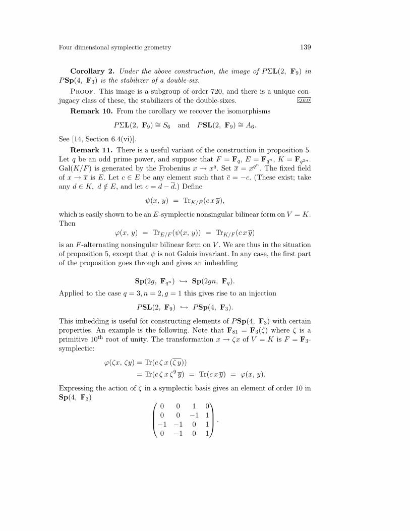
This imbedding is useful for constructing elements of PSp(4, F3) with certainproperties. An example is the following. Note that F81 = F3(ζ) where ζ is aprimitive 10th root of unity. The transformation x → ζx of V = K is F = F3-symplectic:
ϕ(ζx, ζy) = Tr(c ζ x (ζ y))
= Tr(c ζ x ζ9 y) = Tr(c x y) = ϕ(x, y).
Expressing the action of ζ in a symplectic basis gives an element of order 10 inSp(4, F3)
0 0 1 00 0 −1 1−1 −1 0 10 −1 0 1
.

140 J. W. Hoffman, S. H. Weintraub
Now recall that SL(2), as an algebraic group over Fq, has two conjugacyclasses of maximal tori, the split torus T ∼= Gm consisting of the diagonalmatrices, and the anisotropic torus T ′ consisting of the elements of norm 1inside Res
Fq2
Fq(Gm). (Here, norm = NormFq2/Fq
.) Applied to q = 9, we see that
T ′(F9) = elements of norm 1 in F×81
= 〈ζ〉 = the group generated by ζ.
Under the imbedding ResF9F3
(SL(2)) → Sp(4), ResF9F3
(T ′) maps to the maximaltorus T1 of Sp(4) over F3 consisting of the elements of ResF81
F3(Gm) such that
x = x−1, and 〈ζ〉 is the group of F3-rational points of this maximal torus.The same idea applied to the image of T under this imbedding yields ele-
ments of order 8, since T (F9) = F×9 is cyclic of order 8. For example we obtain
in this way the element −1 −1 0 −11 0 0 00 2 0 11 2 1 1
.
The image of ResF9F3
(T ) is also a maximal torus T2 of Sp(4) over F3, isomorphicwith ResF9
F3(Gm). There are three other conjugacy classes of maximal tori in
Sp(4) over a finite field. There is the group of diagonal symplectic matricesT3
∼= Gm×Gm, and there is T4 = T ′×T ′ obtained from the canonical imbeddingSL(2)×SL(2) → Sp(4), where this time T ′ is regarded as a group-scheme overF3. Finally there is T5 = Gm × T ′.
Note that the two explicit matrices we have constructed are in fact inSp(4, Z) and have the same order as their mod 3 reductions.
7. SO(5) picture
We now reinterpret our results in the language of an inner product spaceof dimension 5 over F3. Much of what follows has a large overlap with thework of Edge (see [10, 11, 12]). We will not systematically establish all thepoints of contact between his work and ours, but we will mention some of them.In [11, sect. 16, pp. 141–142] Edge gives a detailed comparison between certainconfigurations he discusses in connection with the geometry of quadrics over F3
and the configurations described by Baker and Todd based on the Burkhardtquartic. In view of the dictionary in section 3., these can then be related toour configurations. Edge uses the language of classical projective geometry inhis work. In what follows we will describe those configurations of interest to us,

Four dimensional symplectic geometry 141
but using the language of modern algebraic geometry. A general introductionto quadrics over finite fields can be found in chapter 5 of [14].
First some generalities on quadrics: We consider a smooth quadric Q ⊂ PN
over a field F of characteristic not equal to 2. This is the locus of zeros of aquadratic form in N + 1 variables, Q(x) = 0. We let Q(x, y) = txQy denotethe associated symmetric bilinear form. Now Q may be regarded as a squarematrix, and then the nonsingularity of the quadric is expressed by detQ = 0.This multiple use of the symbol Q should cause no confusion. For example,x ∈ Q ⇔ Q(x) = 0. Also, we often identify a K-rational point in projectivespace with a vector x ∈ KN+1 that represents it. The points of the quadricQ(x) = 0 are called isotropic vectors (or Q-isotropic vectors). If x /∈ Q, we saythat x is anisotropic; in this case the nonzero value Q(x) is not well defined, butits square-class in K×/ (K×)2 is. If Q(x) belongs to the square-class α, we callx an α-point. In this way we obtain a partition of the anisotropic K-rationalvectors into sets indexed by the square-classes of K. This will only be used herein the case where the ground-field F is a finite field of odd characteristic. Thenthere are only two square-classes, the class of 1 (the squares) and the nonsquares.If Q(x) is a nonzero square, we call x a plus-point ; if it is a nonsquare then wecall it a minus-point. It is clear that the orthogonal group of the quadratic formO(Q) operates so as to preserve the sets of isotropic vectors and of the α-pointsfor any fixed α.
Given a point v ∈ PN , the hyperplane
H(Q, v) = w ∈ PN : Q(w, v) = 0
consists of vectors orthogonal to v, and the intersection
Π(Q, v) = Q ∩H(Q, v)
is called the polar with respect to v. This is a quadric of dimension one less.If v ∈ Q, the polar is the intersection of Q with the tangent plane to Q at v,and is a cone with vertex v. If v /∈ Q then H(Q, v) is transverse to Q and thepolar is nonsingular. The tangent planes TPQ as P varies over Π(Q, v) all passthrough v.
Recall also that if v /∈ Q the map
r(Q, v) : x → x− 2Q(x, v)Q(v, v)
v
is the orthogonal reflection in the plane H(Q, v). It sends v → −v as a vector,hence fixes it in projective space. It fixes the plane H(Q, v) as well.
Our aim is to explicate the isogeny between SO(5) and Sp(4) in geometricform. This discussion is taken from [13, p. 278]. Let V = A4, and let Gr(2, 4)

142 J. W. Hoffman, S. H. Weintraub
be the Grassmannian variety of 2-dimensional vector subspaces of V . This isalso the Grassmannian of lines in P3 = P(V ), sometimes denoted G(1, 3). It isisomorphic to a quadric in P5 = P
(∧2 V), via the Plucker imbedding. If L is
a line generated by vectors x, y, the map is
Gr(2, 4) L → p(L) = (p01, p02, p03, p12, p13, p23)
where
pij =∣∣∣∣xi xj
yi yj
∣∣∣∣ .These satisfy Plucker’s relation
Q(p) = p01p23 − p02p13 + p03p12 = 0
and this gives rise to the isomorphism Gr(2, 4) ∼= Q. All of this works in thecategory of schemes over Z.
If V has a non-degenerate alternating bilinear form ϕ, we can choose a basisin which ϕ is the standard symplectic form, and the condition that L be ϕ-isotropic, ϕ(x, y) = 0, is that p02+p13 = 0. In other words, the variety Iso(V, ϕ)of isotropic 2-planes in V (= maximal isotropic subspaces) is isomorphic withthe quadric q in (p01, p02, p03, p12, p23)-space with equation
q(p) = p202 + p01p23 + p03p12 = 0.
In the language of polars, this can be stated as q = Π(Q, j), where j =(0, 1, 0, 0, 1, 0). If P is the parabolic subgroup of Sp(4) stabilizing a maximalisotropic subspace (in previous notation, P = P (h)), then
Iso(V, ϕ) = Sp(4)/P
where the quotient is understood in the category of sheaves for the flat topology.This works over Spec(Z) for the standard form ϕ.
Let T ∈ Sp(V, ϕ) = Sp(4, F ). Then T acts on (the F -rational pointsof) Gr(2, 4), Iso(V, ϕ), and also ∧2T acts on ∧2V . The Plucker imbedding isequivariant for these actions, and the symplectic group by its definition pre-serves the hyperplane p02 + p13 = 0. This means that we have an action ofSp(4) on (p01, p02, p03, p12, p23)-space preserving the quadric q. This gives a ho-momorphism from the symplectic group to the group of orthogonal similitudesof the form q, but as the symplectic group has no rational character, the imagelands in O(q), and in fact in SO(q) because the symplectic group is connected.We therefore have a homomorphism
Sp(4) −→ SO(q).
Four dimensional symplectic geometry 143
This is is an isogeny with kernel Z/2 (really µ2), the spin covering of the specialorthogonal group. Thus we have an isomorphism of algebraic groups PSp(4) =Sp(4)/µ2
∼= SO(q). Now assume that our ground ring is a perfect field F .Taking F -rational points, we get the exact sequence in Galois cohomology:
0 −→ ±1 −→ Sp(4, F ) −→ SO(q, F ) N−→ H1(Gal(F/F ), Z/2).
The map N is the spinorial norm.This gives an isomorphism
PSp(4, F ) = Sp(4, F )/± 1 ∼= g ∈ SO(q, F ) : N(g) = 1.
Note that we do not have PSp(4, F ) = Sp(4, F )/ ± 1. For instance if F is afinite field the right-hand side in the exact sequence is Z/2, and the image ofPSp(4, F ) is of index 2 inside PSp(4, F ) = SO(5, F ) as the group of elementsof spinorial norm 1. When F = F3 this is a finite simple group, which in thenotations of the Atlas is denoted Ω+
5 (3) = PΩ+5 (3) = O+
5 (3).We will sketch the construction of the reverse correspondence. Let F1,q be
the Fano variety of lines on the 3-dimensional quadric q. It is known that F1,q∼=
P3 = P(V ) as follows. Each line m ⊂ q is a collection lx : x ∈ m of ϕ-isotropiclines lx ⊂ P (V ). In fact, this is the pencil of isotropic lines through a uniquepoint v ∈ P (V ). If v ∈ P (V ) is any point, the hyperplane
H(ϕ, v) = w ∈ P (V ) : ϕ(v, w) = 0
contains v and the isotropic lines through v are exactly the lines through vcontained in the plane H(ϕ, v), and any such hyperplane defines a line in qvia the Plucker imbedding. The isomorphism F1,q
∼= P(V ) sends m to the axisv of the pencil lx : x ∈ m. Now any element of O(q) preserves q, and thelines on it, and therefore induces an automorphism of P(V ) preserving all thehyperplanes H(ϕ, v), therefore giving an element of the group of symplecticsimilitudes, and this gives the map in the other direction
SO(q) = PSO(q) −→ PSp(4).
We have only sketched these arguments, because the equality
Spin(q) ∼= Sp(4)
is classical. One can find a complete proof of the equality in the generalityclaimed here, namely in the category of group schemes over Z, in [21, pp. 28-32].

144 J. W. Hoffman, S. H. Weintraub
We let W = H(Q, j) denote the hyperplane of isotropy, with coordinates(p01, p02, p03, p12, p23).
Next we turn to the nonsingular pairs ∆ = δ, δ⊥. The Plucker coordinatesp(δ), p(δ⊥) lie on Q = Gr(2, 4) but not on the hyperplane of isotropy p02+p13 =0, that is, not on H(Q, j). In fact they are reflected points of each other relativeto this hyperplane, that is
r(Q, j)p(δ) = p(δ⊥)
This is easily seen for δ = span(e1, e3), δ⊥ = span(e2, e4) in a standardsymplectic basis e1, e2, e3, e4, and the general case follows from this becausethe symplectic group acts transitively on the ∆’s. Let w = w(∆) ∈ H(Q, j) bethe unique point of intersection of H(Q, j) with the line connecting p(δ), p(δ⊥).In fact, start with any F -rational point w ∈ H(Q, j)− q and move parallel to jin the space ∧2V until you hit the quadric Q and you get the Plucker coordinatesof a nonsingular pair. This intersection point is of the form w+ t j, and satisfiesQ(w+ t j, w+ t j) = 0. Remembering that Q(w, j) = 0, and Q(j, j) = −1, thisbecomes t2 = q(w, w). As to the field of definition of the vector w(∆) there aretwo possibilities (F a finite field of odd characteristic):
1. w is a plus point. In that case t2 = q(w, w) has a solution in F . Since thePlucker coordinates w = p(δ) are F -rational, the line δ, and also δ⊥, is anF -rational line in V . This ∆ = δ, δ⊥ is what has been previously calleda nonsingular pair, but will now be called a split nonsingular pair.
2. w is a minus point. In that case√q(w, w) defines a nontrivial quadratic
extension E of F . The δ, δ⊥ are a Galois-conjugate pair of E-rational linesin V : δ = δ⊥. We say that ∆ is a twisted, or nonsplit, nonsingular pair.
For example, when F = F3, there are 45 split nonsingular pairs, and 36twisted nonsingular pairs. We will show that these 36 correspond naturally tothe double-sixes.
We denote by ∆(w) = δ(w), δ⊥(w) the nonsingular pair constructed bythe above process from w ∈ H(Q, j) − q. For any such w consider the polarvariety qw := Π(q, w) inside W . Since w = δ + t j and w = δ⊥ − t j for somet = 0, we see that
qw = Q ∩H(Q, δ) ∩H(Q, δ⊥)
where we are using the abbreviation H(Q, δ) = H(Q, p(δ)). This smoothquadric surface is isomorphic over the algebraic closure F to a product of pro-jective lines. This isomorphism does not necessarily hold over the field F . Infact,
Four dimensional symplectic geometry 145
1. w is a plus-point ⇒ qw ∼= P1F × P1
F .
2. w is a minus-point ⇒ qw ∼= ResEF
(P1
E
)where E = F (
√q(w,w)).
Note in particular that qw(F ) is respectively P1(F ) ×P1(F ) and P1(E). Sinceqw ⊂ q = Iso(V, ϕ), the points of these quadrics correspond to certain collectionsof isotropic lines in V . These are easily identified:
1. If w is a plus-point, then ∆(w) = δ, δ⊥ for a pair of F -rational anisotro-pic lines. Take any F -rational points a ∈ δ, b ∈ δ⊥. Then the line ab isisotropic, and the P1(F ) × P1(F ) indexed collection of isotropic lines soobtained is qw(F ). Generalizing this construction to R-valued points forany F -algebra R gives the isomorphism of schemes qw ∼= δ(w) × δ⊥(w).
2. If w is a minus-point, then ∆(w) = δ, δ⊥ for a pair of E-rationalanisotropic lines with δ = δ⊥. Take any E-rational point a ∈ δ. Its Galoisconjugate a lies on δ⊥. The line aa is isotropic, and F - rational since fixedby Galois. The P1(E) indexed collection of isotropic lines obtained in thisway is qw(F ). Generalizing this construction to R-valued points gives theisomorphism of schemes qw ∼= ResE
F (δ(w)) ∼= ResEF
(δ⊥(w)
).
Let us call the lines constructed above cross-lines. Given two distinct cross-lines on a nonsingular pair one of two alternatives holds: either they are skewor they intersect in a point necessarily on ∆. This can be seen as follows: Ifthere were an intersection, not on either δ or δ⊥, the plane spanned by thesecross-lines would contain both δ and δ⊥, since it would contain two points oneach of these. But this contradicts δ ⊕ δ⊥ = V , thinking of the projective linesnow as planes through the origin in V . However, for a twisted nonsingular pair,the second alternative cannot occur. The reason is that the cross-lines are F -rational lines, and hence the intersection, if it existed, would be an F -rationalpoint, and by the previous remark, on δ or δ⊥. But neither δ nor δ⊥ has anyF -rational points because δ ∩ δ = δ ∩ δ⊥ = ∅.
These observations are valid over any field of characteristic not 2, with thenotion of plus and minus points replaced by α-points, but we will only needthis for F3, where the statements above can be verified by direct calculationfor any one representative, the transitivity of the symplectic group giving thegenerality of the claim. It is worth observing that over any finite field of oddcharacteristic, the quadratic forms Q and q are equivalent respectively to Q0 =x2
0 +x21 +x2
2 +x23 +x2
4−x25 and q0 = x2
0 +x21 +x2
2 +x23 +x2
4. The reason for this isthat terms such as uv are equivalent to x2 − y2, so that Q and q are equivalentto sums and differences of squares, and the only invariant of a quadratic formover a finite field aside from its rank is its discriminant, which is −1 for Q and1 for q.
146 J. W. Hoffman, S. H. Weintraub
There are 45 points in P4(F3) where q0(x) = 1 and 36 points where q0(x) =−1. For the plus-point w = (1, 0, 0, 0, 0) the quadric qw is x2
1 +x22 +x2
3 +x24 = 0,
which has 16 points, reflecting qw(F3) = P1(F3)×P1(F3). For the minus-pointw = (1, 1, 0, 0, 0) the quadric qw is 2x2
1 + x22 + x2
3 + x24 = 0, which has 10 points,
reflecting qw(F3) = P1(F9).When F = F3 we will identify the twisted nonsingular pairs with the double-
sixes. Note that in this case each twisted nonsingular pair defines a set of 10cross-lines, all disjoint, each containing four F3-rational points, hence consti-tuting a partition of the 40 points of P3(F3). We could call this an isotropicspread.
We now analyze the concept of an nsp-spread in the orthogonal setting. Firstconsider the vector space W = FN+1 with a quadratic form q. By a base wemean a collection v0, . . . , vN of plus-points of P(W ) such that q(vi, vj) = 0for i = j. This is almost the same thing as an orthonormal basis of W ; we canchoose liftings vi of vi such that q(vi, vi) = 1, and the vi will indeed be anorthonormal basis.
Let F = F3, W = H(Q, j), and let q be the quadratic form given by therestriction of the Plucker relation to the ϕ-isotropic 2-planes, as in the previousparagraphs. As we have mentioned, q is equivalent to a sum of 5 squares. In thiscase there are 27 bases. We will identify them with the 27 nsp-spreads. Recallthe assignment
(P(W ) − q) w → ∆(w) ⊂ P(V ).
We have seen that this maps plus-points to split nonsingular pairs. The followinglemma links the nsp-spreads to the bases:
Lemma 10. 1. Over any field F of characteristic not equal to two, if w1
and w2 are q-anisotropic vectors, then
q(w1, w2) = 0 =⇒ ∆(w1) ∩ ∆(w2) = ∅.
2. Over F = F3, the converse of the above implication is true.Proof. Given two anisotropic lines δ1, δ2 ⊂ P3, we have that δ1 ∩ δ2 =
∅ ⇒ δ⊥1 ∩ δ⊥2 = ∅. Thus given two nonsingular pairs ∆1 = δ1, δ⊥1 and ∆2 =δ2, δ⊥2 , either they are disjoint or they intersect in 2 points, i. e., after possiblyexchanging a line with its dual, δ1∩δ2 = point and δ⊥1 ∩δ⊥2 = point. It is a generalfact about Grassmannians that given two lines l, m ⊂ P3, then l∩m = ∅ if andonly if the line containing their Plucker coordinates p(l), p(m) ∈ Gr(2, 4) = Qis entirely contained in the Grassmannian. Recall also that the line determinedby two points x, y on a quadric Q is contained in Q if and only if they areorthogonal. Hence two lines l, m are incident if and only if Q(p(l), p(m)) = 0,which we will abbreviate as Q(l, m) = 0.
Four dimensional symplectic geometry 147
Thus∆1 ∩ ∆2 = ∅ ⇐⇒ Q(δ1, δ2) = 0 or Q(δ1, δ⊥2 ) = 0.
The vectors w1 = w(∆1) and w2 = w(∆2) in P4 = P(H(Q, j)) are determinedby
wi = δi −Q(δi, j)Q(j, j)
j
where we are identifying a line with its Plucker coordinate. Also
δ⊥i = r(Q, j)δi = δi − 2Q(δi, j)Q(j, j)
j.
One computes
q(w1, w2) = Q(w1, w2) = Q(δ1, δ2) −Q(δ1, j)Q(δ2, j)
Q(j, j). (1)
Since δ1 and δ2 are anisotropic, Q(δ1, j) = 0 and Q(δ2, j) = 0. Notice that theexpression on left-hand side depends only on the orthogonal projections w1, w2
of the vectors δ1, δ2 to the plane H(Q, j). Since δ⊥i has the same projection tothis plane as δi we can replace δi by δ⊥i for i = 1 or 2. We conclude from thisthat
∆1 ∩ ∆2 = ∅ =⇒ q(w1, w2) = 0
The contrapositive of this is part 1 of the lemma.We cannot conclude the converse implication of this in general, but for the
finite field with three elements we reason as follows. From q(w1, w2) = 0 we wishto conclude that Q(δ1, δ2) = 0 or Q(δ1, δ⊥2 ) = 0, hence ∆1 ∩ ∆2 = ∅. A simplecalculation shows that
Q(δ1, δ⊥2 ) = Q(δ1, δ2) +Q(δ1, j)Q(δ2, j)
Q(j, j)(2)
The second summand in both equations 1 and 2 is nonzero, as mentioned. Ifq(w1, w2) = 0 and Q(δ1, δ2) = 0 then the only possibilities for equation 1 are2 − 1 or 1 − 2. But then equation 2 becomes 1 + 2 = 0. QED
An nsp-spread is a mutually disjoint collection of 5 ∆’s, and correspondsby the above to a collection of 5 mutually orthogonal plus - points in the 5-dimensional space W , which is a base by definition. It is clear that the stabilizerin SO(5, F3) of a base consists of the orthogonal matrices generated by thefollowing matrices: the even permutation matrices of size 5, and the diagonalmatrices with ±1 down the diagonal, the product of these being 1. Conjugationby the permutation matrices acts as permutations of the diagonal entries in these

148 J. W. Hoffman, S. H. Weintraub
diagonal generators. This gives a precision of the result in lemma 3, namely thestabilizer of an nsp-spread is the semi-direct product (Z/2)4 A5. Also as analgebraic group it is clear that the stabilizer of a base has the same matriceswith coordinates in any extension of F3, so this stabilizer is the constant group,of dimension 0, with this value.
Finally we describe the double-sixes in the orthogonal language. In thisparagraph, F = F3. The statements that follow were verified by computercalculations. As mentioned before, the quadratic form q is equivalent to asum of 5 squares over any finite field of odd characteristic. We show thatthe minus-points correspond naturally to double-sixes. Let B = e1, . . . . , e5be one of the 27 bases. This is essentially an orthonormal basis for q. Letw = w(∆) = (w1, . . . , w5) ∈ F5
3 be a minus-point, expressed in this basis;given B, the coordinates wi are ambiguous only up to ±wi and permutations.Since q(w) = w2
1 + . . . + w25 = 2 mod 3, it is clear that one of two possibilities
occur: (1) exactly two vectors ei in B have q(w, ei) = 0 or (2) all five vectors inB have q(w, ei) = 0. If the first case occurs then we say that B is a 2-base rela-tive to w, and in the second case that B is a 5-base relative to w. Given w thisgives a division of the 27 bases into the 2-bases and the 5-bases. It is clear thatthe stabilizer subgroup of w inside O(5, F3) preserves this partition into 2- and5-bases relative to w. For any minus-point there are fifteen 2-bases and twelve5-bases. We claim that the twelve 5-bases arrange themselves into a double-six.In fact, consider the orthogonal reflection in the hyperplane H(q, w) ⊂ P4(F3).This orthogonal transformation fixes w and hence acts on the twelve 5 - bases.This involution acts fixed-point free on the twelve and the orbits
B1, B′1, B2, B
′2, B3, B
′3, B4, B
′4, B5, B
′5, B6, B
′6
are the six doublets in a double-six. Let us call the projective involutions inducedby these θw. They are elements of the group denoted PGO5(3) in the Atlas. Weremark that these 36 involutions, one for each minus-point, are exactly the 36F -inversions that appear in [11, p. 145].
Here is another observation, due to Edge (see also [14, Section 6.4(ii)] and [15,Theorem 15.3.17]):
Proposition 6. There are isomorphisms: PGO−4 (3) ∼= S6 and PSO−
4 (3) ∼=A6.
This appears in [10, p. 277]. Recall that PGO−4 (3) is the group of projective
transformations induced from the linear transformations that preserve a non-degenerate quadratic form in 4 variables over F3 of Witt defect 1. Here we arefollowing the notations and terminology of the Atlas.
Proof. We have already (see corollary 2 and remark 10) shown that thestabilizer inside G = Ω+
5 (3) of a double-six is isomorphic with the symmetric

Four dimensional symplectic geometry 149
group S6. We have identified the double-sixes with the minus points in the spaceF5
3 with the quadratic form q = x21+x2
2+x23+x2
4+x25. Let w be any minus-point,
eg. (1, 1, 1, 1, 1). Then any element in the stabilizer Gw of w in G will fix thehyperplane H(q, w) orthogonal to w, and induce an element in the orthogonalgroup of the quadratic form q|w obtained by restricting q to H(q, w). It iseasily checked that q|w has Witt defect 1, so we have a map Gw → PGO−
4 (3).This maps the subgroup A6
∼= G′w consisting of elements of determinant one to
PSO−4 (3). These two groups have the same cardinality, so it is an isomorphism
by simplicity of A6, and one also sees the isomorphism Gw∼= PGO−
4 (3). QED
We can summarize the results of this section as the Sp(4) ∼ SO(5) -equivariant identifications in the table below. The stabilizers are algebraic sub-groups in Sp(4), and their dimensions are given.
symplectic orthogonal stabilizer dimensionisotropic line point of q parabolic P (h) 7
point line in q parabolic P (l) 7split ns. pair plus-point (SL(2) × SL(2)) Z/2 6
twisted ns. pair/dbl 6 minus-point ΣLF9/F3(2) 6
nsp-spread base 2.((Z/2)4 A5
)0
8. The Weyl group of E6
In Coxeter [6], which is based on Edge [12], an isomorphism is establishedbetween the group SO−
6 (2) and the Weyl group of the root system E6. One alsoknows that this group is isomorphic with PGO5(3).This “exceptional” isomor-phism will be explained below, but for now, we can identify the 36 involutionscorresponding to the root hyperplanes in the root system E6: they are the 36involutions associated to the minus-points in our discussion of double-sixes inthe previous section. We can also identify a set of six involutions correspondingto a basis for the root-system. Coxeter shows how to construct involutions hecalls Ri, i = 1, . . . , 6, associated to the nodes of the Dynkin diagram, and heidentifies them with their action on the 27 lines on a cubic surface.
In a classical notation, these 27 lines are labeled ai, bi, cij , 1 ≤ i, j ≤ 6,i < j. This notation presupposes a basic double-six has been chosen and the(ai, bi) i = 1, . . . , 6 are the doublets in this double-six. For instance, take for areference double-six entry 11 of Table 3. Thus, in the lexicographic ordering ofthe indices,
ai = 1, 6, 8, 14, 22, 27bi = 5, 7, 3, 24, 26, 13cij = 4, 2, 20, 18, 10, 9, 16, 11, 21, 12, 19, 17, 23, 15, 25
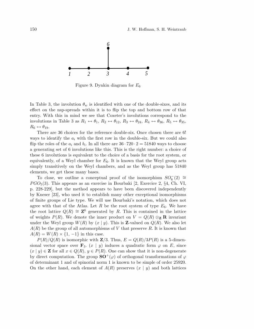
150 J. W. Hoffman, S. H. Weintraub
1 2 3 4 5
6
Figure 9. Dynkin diagram for E6
In Table 3, the involution θw is identified with one of the double-sixes, and itseffect on the nsp-spreads within it is to flip the top and bottom row of thatentry. With this in mind we see that Coxeter’s involutions correspond to theinvolutions in Table 3 as R1 ↔ θ1, R2 ↔ θ12, R3 ↔ θ24, R4 ↔ θ36, R5 ↔ θ35,R6 ↔ θ19.
There are 36 choices for the reference double-six. Once chosen there are 6!ways to identify the ai with the first row in the double-six. But we could alsoflip the roles of the ai and bi. In all there are 36 · 720 · 2 = 51840 ways to choosea generating set of 6 involutions like this. This is the right number: a choice ofthese 6 involutions is equivalent to the choice of a basis for the root system, orequivalently, of a Weyl chamber for E6. It is known that the Weyl group actssimply transitively on the Weyl chambers, and as the Weyl group has 51840elements, we get these many bases.
To close, we outline a conceptual proof of the isomorphism SO−6 (2) ∼=
PGO5(3). This appears as an exercise in Bourbaki [2, Exercice 2, §4, Ch. VI,p. 228-229], but the method appears to have been discovered independentlyby Kneser [23], who used it to establish many other exceptional isomorphismsof finite groups of Lie type. We will use Bourbaki’s notation, which does notagree with that of the Atlas. Let R be the root system of type E6. We havethe root lattice Q(R) ∼= Z6 generated by R. This is contained in the latticeof weights P (R). We denote the inner product on V = Q(R) ⊗Z R invariantunder the Weyl group W (R) by (x | y). This is Z-valued on Q(R). We also letA(R) be the group of all automorphisms of V that preserve R. It is known thatA(R) = W (R) × 1, −1 in this case.
P (R)/Q(R) is isomorphic with Z/3. Thus, E = Q(R)/3P (R) is a 5-dimen-sional vector space over F3. (x | y) induces a quadratic form ϕ on E, since(x | y) ∈ Z for all x ∈ Q(R), y ∈ P (R). One can show that it is non-degenerateby direct computation. The group SO+(ϕ) of orthogonal transformations of ϕof determinant 1 and of spinorial norm 1 is known to be simple of order 25920.On the other hand, each element of A(R) preserves (x | y) and both lattices
Four dimensional symplectic geometry 151
P (R), Q(R). Thus we obtain a homomorphism λ : A(R) → O(ϕ). One checksby direct computation that the reduction map Q(R) → E is carries R bijectivelyonto its image, from which it easily follows that λ is injective. A comparison oforders shows that it is an isomorphism.Thus λ(W (R)) is a subgroup of O(ϕ) ofindex 2. The group O(ϕ)/SO+(ϕ) is of type (2, 2). The subgroups of index 2are
±1 × SO+(ϕ), SO(ϕ), Ω(ϕ)
the last group being characterized by being of index two, not contained inSO(ϕ), and not containing −1. Clearly this is isomorphic with PO(ϕ). Notethat Ω(ϕ) is isomorphic with the group we have denoted by G in section 2.. Thisis the image of W (R) under λ, because reflections have determinant −1 and itis known that −1 /∈W (R) (see [2, p. 220]). Note also that λ maps the subgroupW+(R) of W (R) consisting of elements of determinant 1 isomorphically ontoSO+(ϕ).
Now let F = Q(R)/2Q(R), which is an F2-vector space of dimension 6. Oneverifies that 1
2(x | y) defines a non-degenerate quadratic form q6 on F . As beforewe obtain a homomorphism µ : A(R) → O(q6). Visibly, −1 is in the kernel. Weclaim that this generates the kernel, and thus we have an isomorphism of W (R)with O(q6). Perhaps the easiest way to see this is to note that the restrictionto W+(R) is nontrivial, hence injective by simplicity of this group. The imageis the subgroup of index 2, O+(q6). Then each reflection maps to a reflectionin F . In fact, if R denoted the set of equivalence classes of R for the relationr ∼ −r, µ maps R isomorphically onto its image in F . As W (R) is generatedby W+(R) and any reflection, this shows that W (R) maps onto all of O(q6),hence isomorphically onto it, by a comparison of orders.
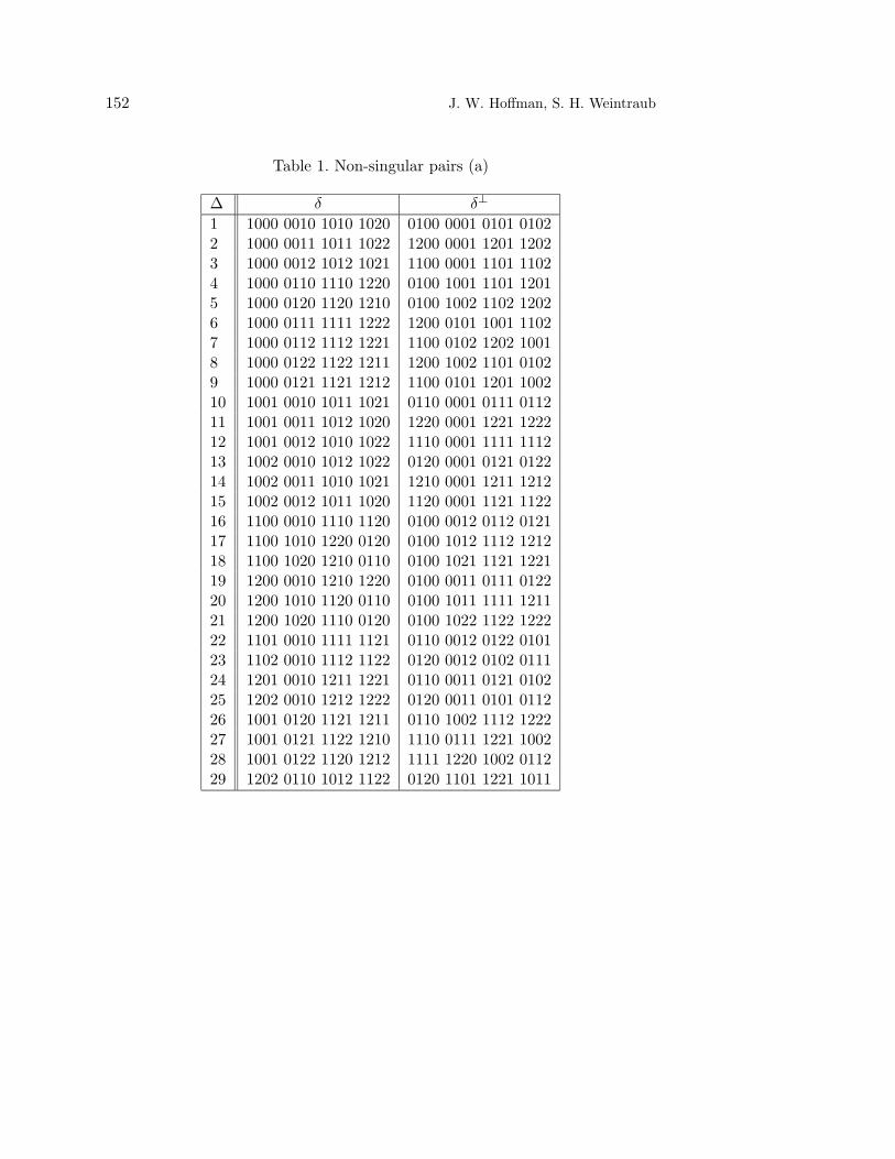
152 J. W. Hoffman, S. H. Weintraub
Table 1. Non-singular pairs (a)
∆ δ δ⊥
1 1000 0010 1010 1020 0100 0001 0101 01022 1000 0011 1011 1022 1200 0001 1201 12023 1000 0012 1012 1021 1100 0001 1101 11024 1000 0110 1110 1220 0100 1001 1101 12015 1000 0120 1120 1210 0100 1002 1102 12026 1000 0111 1111 1222 1200 0101 1001 11027 1000 0112 1112 1221 1100 0102 1202 10018 1000 0122 1122 1211 1200 1002 1101 01029 1000 0121 1121 1212 1100 0101 1201 100210 1001 0010 1011 1021 0110 0001 0111 011211 1001 0011 1012 1020 1220 0001 1221 122212 1001 0012 1010 1022 1110 0001 1111 111213 1002 0010 1012 1022 0120 0001 0121 012214 1002 0011 1010 1021 1210 0001 1211 121215 1002 0012 1011 1020 1120 0001 1121 112216 1100 0010 1110 1120 0100 0012 0112 012117 1100 1010 1220 0120 0100 1012 1112 121218 1100 1020 1210 0110 0100 1021 1121 122119 1200 0010 1210 1220 0100 0011 0111 012220 1200 1010 1120 0110 0100 1011 1111 121121 1200 1020 1110 0120 0100 1022 1122 122222 1101 0010 1111 1121 0110 0012 0122 010123 1102 0010 1112 1122 0120 0012 0102 011124 1201 0010 1211 1221 0110 0011 0121 010225 1202 0010 1212 1222 0120 0011 0101 011226 1001 0120 1121 1211 0110 1002 1112 122227 1001 0121 1122 1210 1110 0111 1221 100228 1001 0122 1120 1212 1111 1220 1002 011229 1202 0110 1012 1122 0120 1101 1221 1011

Four dimensional symplectic geometry 153
Table 1. Non-singular pairs (b)
∆ δ δ⊥
30 1102 0110 1212 1022 0120 1201 1021 111131 1222 0121 1010 1101 1012 0101 1110 121132 1201 0112 1010 1122 1110 0102 1212 101133 1102 0122 1221 1010 1210 1012 1111 010234 1020 0121 1111 1202 1120 0101 1221 102235 1020 0111 1101 1212 1220 0101 1021 112236 1010 0111 1121 1202 1210 0101 1011 111237 1200 0012 1212 1221 1100 0011 1111 112238 1202 0012 1211 1220 1101 0011 1112 112039 1201 0012 1210 1222 1102 0011 1110 112140 1020 0112 1102 1211 1120 0102 1222 102141 1020 0122 1112 1201 1220 0102 1022 112142 1200 0112 1012 1121 1100 1011 1222 012243 1200 0121 1021 1112 1100 1022 1211 011144 1101 0112 1210 1022 1110 0122 1202 102145 1201 1012 1120 0111 1102 1011 1220 0121

154 J. W. Hoffman, S. H. Weintraub
Table 2. Nsp-spreads
σ ∆1 1 26 37 44 452 1 27 30 38 423 1 28 29 39 434 2 16 26 33 355 2 17 22 27 406 2 18 23 28 317 3 19 26 32 348 3 20 25 27 419 3 21 24 28 3610 4 13 36 37 4011 4 14 23 34 4212 4 15 25 33 4313 5 10 31 37 4114 5 11 22 32 4315 5 12 24 35 4216 6 13 18 32 3817 6 14 16 29 4118 6 15 17 24 4419 7 13 20 35 3920 7 14 21 22 4521 7 15 19 30 3122 8 10 17 34 3923 8 11 16 30 3624 8 12 18 25 4525 9 10 21 33 3826 9 11 20 23 4427 9 12 19 29 40

Four dimensional symplectic geometry 155
Table 3. double-sixes
θ doublets θ doublets1 1 5 9 11 16 21 19 2 4 9 14 22 27
6 7 2 18 20 10 7 3 5 25 15 232 1 5 11 19 23 25 20 2 6 10 14 17 22
22 26 4 2 20 10 13 23 3 11 5 163 1 5 15 17 21 25 21 2 6 14 18 19 27
27 13 20 2 4 18 26 15 21 3 5 164 1 6 8 15 23 25 22 2 9 12 13 19 27
9 2 4 26 13 24 10 21 15 3 25 85 1 6 12 19 23 27 23 3 7 13 18 20 23
21 10 26 24 3 4 21 17 9 14 22 16 1 8 11 14 21 25 24 2 9 14 17 19 24
12 20 13 2 26 7 20 16 8 15 23 37 1 8 15 16 21 22 25 4 8 10 14 21 22
19 18 7 13 24 2 13 23 7 19 5 128 1 9 12 16 22 27 26 4 8 16 20 22 27
25 24 7 3 10 18 24 25 5 7 17 199 1 6 12 15 17 22 27 4 9 11 14 21 24
11 18 13 3 24 4 20 12 23 6 15 710 2 4 10 14 18 24 28 4 8 11 14 18 27
12 16 15 1 23 5 26 15 5 17 7 1211 1 6 8 14 22 27 29 4 9 11 13 16 27
5 7 3 24 26 13 10 17 25 7 15 612 2 6 7 12 17 19 30 5 9 12 13 16 26
4 8 3 16 21 11 25 14 6 18 8 1013 2 6 12 20 22 27 31 5 9 11 13 19 24
24 25 5 3 21 11 15 22 8 20 6 1014 2 7 10 17 24 26 32 6 7 18 19 23 25
27 23 8 1 11 16 22 26 4 9 16 2115 1 9 11 14 19 27 33 5 9 17 21 24 26
15 26 3 10 7 20 23 27 6 8 18 2016 2 9 12 17 22 26 34 10 14 17 21 24 25
18 11 23 25 8 3 20 27 12 16 13 2317 3 4 8 10 18 20 35 11 13 18 19 23 27
5 9 1 17 19 12 21 26 10 17 15 2218 1 6 14 17 19 25 36 11 14 18 19 24 25
16 20 4 26 13 3 16 22 20 12 26 15

156 J. W. Hoffman, S. H. Weintraub
References
[1] H. F. Baker: A locus with 25920 linear self-transformations, Cambridge tracts in Math-ematics and Mathematical Physics 39, Cambridge University Press, 1946.
[2] N. Bourbaki: Groupes et Algebres de Lie, Chaptaires 4, 5, et 6, Elements deMathematique, Masson, 1981.
[3] H. Burkhardt: Untersuchungen aus dem Gebiet der hyperelliptischen Modulfunctionen(I), Math. Ann. 36 (1890), 371–434.
[4] H. Burkhardt: Untersuchungen aus dem Gebiet der hyperelliptischen Modulfunctionen(II), Math. Ann. 38 (1891), 161–224.
[5] H. Burkhardt: Untersuchungen aus dem Gebiet der hyperelliptischen Modulfunctionen(III), Math. Ann. 41 (1893), 313–343.
[6] A. B. Coble: A configuration in finite geometry isomorphic with that of the twenty-sevenlines of a cubic surface, Johns Hopkins Univ. Circ., 7 (1908), 80–88.
[7] J. H. Conway, R. T. Curtis, S. P. Norton, R. A. Parker, R. A. Wilson: Atlas offinite groups, Oxford University Press, 1985.
[8] H. S. M. Coxeter: Polytopes over GF(2) and their relevance for the cubic surface group,Canad. J. Math. 11 (1959), 646–650.
[9] L. E. Dickson: Determination of all the subgroups of the known simple group of order25920, Trans. Amer. Math. Soc. 5 (1904), 126–166.
[10] W. L. Edge: Geometry in 3 dimensions over GF(3), Proc. Roy. Soc. London (A), 222(1954), 262–286.
[11] W. L. Edge: Line geometry in three dimensions over GF(3) and the allied geometry ofquadrics in four and five dimensions, Proc. Roy. Soc. London(A) 228 (1955), 129–146.
[12] W. L. Edge: Quadrics over GF(2) and their relevance for the cubic surface group, Canad.J. Math. 11 (1959), 625–645.
[13] W. Fulton J. Harris: Representation Theory. A first course, Graduate Texts in Math.129, Springer–Verlag, 1991.
[14] J. W. P. Hirschfeld: Projective Geometries over Finite Fields, Second Edition, Oxford:Clarendon Press, 1998.
[15] J. W. P. Hirschfeld: Finite Projective Spaces of Three Dimensions, Oxford: ClarendonPress, 1985.
[16] J. W. P. Hirschfeld, J. A. Thas: General Galois Geometries, Oxford: Clarendon Press,1991.
[17] J. W. Hoffman, S. H. Weintraub: The Siegel modular variety of degree two and levelthree, Trans. A. M. S. vol. 353 (2001) n. 8, 3267–3305.
[18] J. W. Hoffman, S. H. Weintraub: Spreads of nonsingular pairs in symplectic vectorspaces, to appear.
[19] K. Hulek, C. Kahn, S. H. Weintraub: Moduli spaces of abelian surfaces: Compacti-fications, degenerations and theta functions, Walter de Gruyter, Berlin, New York, 1993.
[20] B. Hunt: The geometry of some special arithmetic quotients of bounded symmetricdomains, Lecture Notes in Math. 1637, Springer–Verlag, 1996.
[21] J. Hurrelbrink: Isomorphismen von Spingruppen, Gottingen, 1970.

Four dimensional symplectic geometry 157
[22] C. Jordan: Traite des substitutions, Gauthiers–Villars, Paris, 1870.
[23] M. Kneser: Uber die Ausnahme-Isomorphismen zwischen endlichen klassischen Gruppen,Abh. Math. Sem. Univ. Hamburg, 31 (1967), 136–140.
[24] R. Lee, S. H. Weintraub: On the transformation law for theta-constants, J. Pure Appl.Alg., 44 (1987), 273–285.
[25] J. Schwermer: On arithmetic quotients of the Siegel upper half space of degree two,Compositio Math. 58 (1986), 233–258.
[26] J. A. Todd: On the simple group of order 25920, Proc. Royal Soc. London (A), 189(1947), 326–358.
[27] B. L. van der Waerden: Algebra, Springer - Verlag, 1991.