1

Four centuries of return predictability

Benjamin Golez†

University of Notre Dame

Peter Koudijs‡ Stanford University

This version: February 1, 2016

Abstract

We analyze aggregate market prices and dividends throughout modern financial history. Focusing on the most important market in each period, we start with the Dutch and English markets in the early 17th century and move to the U.S. market at the end of the 19th century. We find that the dividend-to-price ratio predicts returns throughout all four centuries. “Excess volatility” is thus a pervasive feature of financial markets. The dividend-to-price ratio also predicts dividend growth rates in all but the most recent (post 1945) period. Cash-flow news was therefore much more important for price movements in the past, and the dominance of discount rate news is a relatively recent phenomenon. We show that this is consistent with an increase in the duration of the stock market in the recent period. Key words: Dividend-to-price ratio, return predictability, dividend growth predictability, duration JEL classification: G12, G17, N2 †256 Mendoza College of Business, University of Notre Dame, Notre Dame, IN 46556, USA, Tel.: +1-574-631-1458, bgolez@nd.edu ‡655 Knight Way, Stanford Graduate School of Business, Stanford, CA 94305, Tel.: +1-650-725-1673, koudijs@stanford.edu *We thank Jules van Binsbergen (discussant), John Campbell (discussant), Anna Cieslak, Zhi Da, Monika Piazzesi, Martin Schneider, Robert Stambaugh (discussant), Stijn Van Nieuwerburgh (discussant), Jessica Wachter, Michael Weber (discussant), Nicholas Hirschey (discussant) and seminar participants at University of Notre Dame, University of California San Diego, Stanford University, European Central Bank, University of Konstanz, 2014 SITE Conference, 2015 Rodney L. White Center for Financial Research Conference, 2015 WFA Conference, 2016 AEA Conference, and 2016 European Winter Finance Conference for comments and suggestions. We thank Gary Shea for generously sharing his data about 18th century British companies, John Turner for his advice on how to use British information from the 19th century, and Manisha Goswami and Cathy Quiambao for research assistance.

2

1. Introduction

One of the most important questions in asset pricing is whether prices (or rather the

dividend-to-price ratio) can predict returns. If so, asset prices would be “excessively volatile;”

that is, they move more than is warranted by fundamentals, such as dividends (Shiller 1981;

LeRoy and Porter 1981). The empirical evidence suggests that returns are indeed partially

predictable (Campbell and Shiller 1988; Fama and French 1988; Cochrane, 2008; Binsbergen

and Koijen 2010). This has motivated an important theoretical literature that incorporates time-

varying returns in equilibrium models (Campbell and Cochrane 1999; Bansal and Yaron 2004;

Albuquerque, Eichenbaum, and Rebelo 2014).

Two issues remain. First, in the recent period, the dividend-to-price ratio is highly

persistent, virtually indistinguishable from a unit root. Combined with the relatively short

sample, this biases estimates in favor of finding return predictability (Stambaugh 1999). Second,

the existing evidence not only suggests that returns are predictable, it also indicates that dividend

growth rate predictability is limited (Campbell and Shiller 1988; Campbell 1991; Cochrane

1992; 2008; 2011). This implies that “excess volatility” is extreme: prices seem to move only in

response to changing expected returns and not to news about future dividends. The jury is still

out on what can explain this feature of the data.

In this paper we extend the time series of asset prices and dividends to cover the whole

history of modern financial markets starting in 17th century Amsterdam. In particular, we focus

on the dominant stock markets of the time: the Dutch stock market in the 17th and 18th century,

the U.K. stock market in the 18th and 19th century, and the U.S. stock market from the end of the

19th century onwards. With this focus, we cover a large fraction of global market capitalization.

The included companies are very similar to those of today, with limited liability for shareholders,

3

separation of ownership and control, and an active secondary market for shares. By extending the

time series, we add independent variation to the data. This is more difficult to achieve in the

cross-section, where markets often move together, especially in the recent period.

The paper has four key findings. First, across all four centuries, the dividend-to-price

ratio is stationary, fluctuating around a long-run average of five percent (minus three in logs, see

Figure 1 for details). It is only after around 1945 that the dividend-to-price ratio starts to

persistently decrease. This is interesting in its own right, but also means that, for the period as a

whole, results are not biased due to a non-stationary predictor. Although the dividend-to-price

ratio has decreased in the recent period1, expected returns have been approximately stable over

time, with returns increasingly coming from capital appreciation in lieu of decreasing dividends.

Second, we find robust evidence for return predictability. In the full period covering all

four centuries, the predictive coefficient on the dividend-to-price ratio is positive and highly

significant, for both annual and multiannual horizons. In subperiods, the predictive coefficient is

remarkably stable, although not always statistically significant. Thus, excess volatility appears to

be a pervasive characteristic of financial markets.

Third, there are important differences between periods in terms of dividend growth

predictability. While the dividend-to-price ratio strongly predicts dividend growth rates in the

earlier periods, such predictability completely disappears around 1945. In line with this

observation, our analysis implies that, before 1945, changes in cash-flows were more important

for price movements than changes in discount rates. The dominance of discount rate news is

therefore a relatively recent phenomenon.

1 This decrease is also present in the data when we account for share repurchases and issuances. Net payout has fallen even more dramatically after 1945 than the dividend-to-price ratio.

4

Fourth, return predictability is concentrated in recession periods - more so than dividend

growth rate predictability. This suggests that, in comparison to expansions, discount rate news is

more important than cash flow news during recessions.

All in all, our analysis reveals that returns have always been predictable, especially in

downturns. At the same time, the recent (post 1945) period stands out with a very low dividend-

to-price ratio and a dominant role for discount rate news. We hypothesize that this is closely

linked to a recent decrease in the payout ratio (dividends/earnings) and a resulting increase in

stock market duration. In particular, as the payout ratio decreases, companies reinvest a larger

share of their earnings and push cash flow distributions into the future. This increases the

duration of the stock market and suggests that nowadays companies can be seen as longer-lived

high duration assets. As such, they have lower valuation ratios and, as long as expected returns

are more persistent than dividend growth rates, prices are more prone to changes in discount

rates. We illustrate this intuition with a simple stylized present value model where the market

consists of finitely lived companies.

Consistent with our hypothesis, we also show empirically that in the post-1945 period,

the discounted value of the next ten years of (expected) dividends accounts for a significantly

smaller portion of current stock valuations than in earlier periods. Using one minus this

discounted value as a proxy for stock duration, we find that it is highly correlated with the

importance of discount rate news.

Although these results are supportive of our hypothesis, other explanations put forward in

the literature may also play a role. Chen, Da, and Priestly (2012) argue that dividend smoothing

may bias results towards discount rate news. Our tests suggest that both dividend smoothing and

stock duration matter, although stock duration explains a much larger fraction of discount rate

5

news variation. In addition, we document that dividend smoothing in the earlier part of our

sample was comparable to today.

Our paper relates to a large literature on the importance of dividend growth and discount

rates for stock prices. See Koijen and Van Nieuwerburgh (2011) for an overview. Most closely

related are Goetzmann, Ibbotson, and Peng (2001), Chen (2009), and Rangvid, Schmeling, and

Schrimpf (2014). Using primary sources, Goetzmann et al. estimate an index for the New York

stock market between 1815 and 1925. They find little evidence for return predictability, but due

to data limitations, they have to approximate dividends for the period before 1870. Chen

examines the differences between the pre- and post-1945 U.S. periods and argues that before

1945 returns were not predictable, assigning almost all variation in the dividend-to-price ratio to

expected dividend growth rates. In comparison, we show that both returns and dividend growth

rate are predictable in the full period extending 310 annual observations. Also, we note that the

VAR return predictive coefficient in the pre-1945 U.S. period is not statistically different from

the full period. Finally, Rangvid et al. show that discount rates are less important in countries

with relatively small companies and less dividend smoothing.

Our paper is also related to a growing literature that emphasizes the predictability of

dividend growth rates (Menzly, Santos, and Veronesi 2004; Lettau and Ludvigson 2005;

Cochrane 2008; Binsbergen and Koijen 2010; Golez 2014). Relative to this literature, we provide

a long term perspective on the sources of asset price movements that help us understand why

discount rate news dominates in the recent period. Finally, our paper is related to le Bris,

Goetzmann, and Pouget (2014), who analyze six hundred years of dividend and price data for the

Bazacle Company in France. In line with le Bris et al. we show that the dividend-to-price ratio is

stationary, fluctuating around a long run average of 5%.

6

2. Data

We extend the time series of stock prices and dividends back in time until 1629 using the

most important financial markets of a specific period. In particular, for the period between 1629

and 1811, we focus on the equity market in Amsterdam (that included a number of English

securities). For 1825-1870, we look at London. For the period after 1870, we rely on U.S. market

data. In total, we construct an annual time series from 1629 to 2012, with only a small gap for the

years between 1811 and 1825.

While the American data have been extensively studied, the Dutch and English data have

received limited attention in the literature and merit closer inspection. We are the first to look at

return and dividend growth rate predictability in these markets.

During the 17th and 18th century, Amsterdam was the financial capital of the world, and it

was closely integrated with the London market (Neal 1990). Although technologically less

advanced, the market functioned much like the one today. Harrison (1998) provides evidence

that returns in these markets had similar distributions and time series properties as today. Koudijs

(2014) shows that the Amsterdam market responded to the arrival of news in an efficient way

and that trading costs were very similar to the recent period. The (negative) autocorrelation of

returns on a daily level is comparable to today. We take the perspective of an Amsterdam

investor, assuming that he held a value-weighted portfolio of Dutch and English securities. We

use exchange rate information to convert returns in Pounds Sterling into Dutch Guilder returns.2

There is information available for five securities: the Dutch East India Company (from 1629

onwards), the Bank of England (1694), the (United) British East India Company (1693), the

2 Since both England and the Dutch Republic were on metallic standards, exchange rate fluctuations were only of minor importance.

7

South Sea Company (1711), and the (Second) Dutch West India Company (1719). Details on

data sources are provided in Appendix A.

The Dutch East India Company (VOC) was the world’s first publicly traded corporation;

its shares were freely tradable, and shareholders enjoyed limited liability. There was a clear

separation between ownership and control. The Company was founded in 1602, and its capital

became permanent in 1613 (Gelderblom, De Jong, and Jonker 2013). It held the Dutch monopoly

on trade with Asia and operated an extensive trade network there. It started to pay annual

dividends in 1685; before that it paid dividends every two to three years.3 The company was

nationalized by the government in 1796. One of the contributions of this paper is the collection

from the original sources of a complete VOC price series for the years between 1629 and 1719.

The Dutch West India Company (WIC) was founded in 1675 and was involved in slave

trade and the administration of (slave) colonies in Africa and Caribbean. It paid out dividends

sporadically and was nationalized in 1791. Price information is only available for 1719 onwards.

In that year it constituted only one percent of our index, so the omission of the WIC during 1675-

1718 probably has little impact on our estimates.

The Bank of England (BoE) was founded in 1694 to help finance the English government

debt. It held an effective monopoly over issuing banknotes and provided short-term credit to

merchants and banks. It was also an important lender to the British East India Company (EIC).

The EIC was created in 1708 through a merger of the Old and New East India Companies

(between 1693 and 1707 we use the prices of the Old EIC). It held the English monopoly on

trade with Asia. The South Sea Company (SSC) started in 1711 after receiving a monopoly on

the trade with South America. These activities never materialized, and the Company was mainly

3 It is impossible to calculate annual dividend growth rates and dividend-to-price ratios for the VOC up to 1684. Since it is the only company in our sample for that period, we can only run our annual regressions for the years after 1684.

8

a vehicle to finance the English government debt. It performed a number of debt-for-equity

swaps; the final one resulted in the South Sea Bubble in 1720. In that year the company accounts

for 60% of our value-weighted index. After the bubble burst, the company was largely

liquidated; in 1732, it constituted only 6% of our index. Remaining shares were mainly backed

by government debt. It matters very little for our results whether or not we keep the company in

our index after 1732. The English companies have a complicated history of capital calls, rights

issues, and other “capital events.” We use the work by Shea (in preparation) to adjust stock

prices where necessary.

It is important to note that, even though these are only five securities, they effectively

constitute the universe of traded equities in Amsterdam and London. Only during the bubble year

of 1720 did new equities enter the market; most of these new companies were liquidated before

the end of the year (Frehen, Goetzmann, and Rouwenhorst 2013). The few surviving companies

were relatively small and were not widely traded.

The companies in our index were quite large: the total market capitalization to GDP of

securities held by Dutch investors ranged from 15% (during the 1630s and again in the early

1800s) to 64% (during the 1720s).4 This means that diversification was provided within

companies, rather than between them. In comparison, for the U.S., stock market capitalization

amounted to 39% of GDP in 1913 and 152% in 1999 (Rajan and Zingales 2003). In addition,

4 To compute these numbers we use the GDP of Holland, the only Dutch region for which reliable figures are available for the 17th and 18th centuries (Van Zanden and Van Leeuwen 2012). Holland was the largest province of the Dutch Republic, comprising the most populous and developed parts of the country, including important cities like Amsterdam and Rotterdam. The historical evidence suggests that most Dutch investors lived in this area. We used information from Bowen (1989) and Wright (1997) to calculate what fraction of English securities were held by Dutch investors.

9

there were many investment opportunities available outside the stock market such as shipping,

trade and small manufacturing that would have expanded the efficient portfolio frontier.5

For the period between 1825 and 1870 we focus on the London market. After the

Napoleonic Wars, London became the financial capital of the world, and the United Kingdom

was the largest economy in the world. Starting in the 1810s many new equities were issued.

Initially, these were mainly canals and insurances companies. Later on, banks and railroad

companies became the most important issuers of new equity. The period covers the so-called

Railroad “Manias” of the 1830s and 1840s. It is important to note that before 1855, the newly

issued companies had full shareholder liability. Afterwards, it became possible to issue shares

with limited liability, but many banks and insurance companies continued to maintain full

liability.

We use the value-weighted stock market index constructed by Acheson, Hickson, Turner,

and Ye (2009) (henceforth, AHTY) that includes all regularly traded domestic equities traded in

London starting in 1825. The index covers between 125 (1825) and 250 (1870) different

securities. Total market capitalization accounted for between 10 and 30 percent of British GDP.

During this period, there were many new issues and delistings. AHTY (2009) omits all securities

that were traded for less than 12 months (most of these companies failed to raise sufficient

capital to start their businesses) and adjust for survivorship bias by reconstructing companies’

value at liquidation or delisting. In addition, there were many capital calls, rights issues, and

other capital events. AHTY (2009) omits individual security returns for the months in which

these events took place. See AHTY (2009) and Hickson, Turner, and Ye (2011) for more details.

5 Although the overall riskiness of a portfolio depends on diversification possibilities, it should not affect return or dividend growth predictability.

10

Starting in 1871, we rely on the U.S. stock market. By 1900, U.S. had become the largest

economy of the world, with a well-developed capital market in New York. We obtain the data

from Amit Goyal’s webpage. For the period between 1871 and 1925, these data rely on

information from Cowles (1939) that covers between 50 (1871) and 258 (1925) securities. From

1926, the data are based on the S&P 500 index provided by CRSP. Before 1957, this was

actually the S&P 90. As before, our U.S. return index is value-weighted.

3. Methodology

As is standard in the asset pricing literature, we take the perspective of an individual

investor who is interested in the per share value of a company. An investor receives dividends as

the only source of cash-flows. Other types of distributions (e.g. repurchases) are assumed to be

reinvested in the company.6

3.1 Present value relations

The holding period return per share of equity consists of the dividend yield and any price

appreciation:

1

,t tt

t

P DR

P

(1)

where Pt is the per share price at time t and Dt are the per share dividends accumulated from t-1

to t. We take logs and define the dividend-to-price ratio as log( / )t t tdp D P and the dividend

growth rate as 1log( / )t t tdg D D . Using a first-order Taylor expansion around the long-run

6 See Section 5.1 for a discussion on an alternative approach pursued by Larrain and Yogo (2008), which takes the perspective of a representative investor interested in the value of the whole company.

11

mean of the dividend-to-price ratio d p , Campbell and Shiller (1988) show that log returns can

be expressed as:

1 1 1,t t t tr dp dg dp (2)

where all variables are demeaned and exp( ) / 1 exp( )dp dp is the linearization constant.

Rewriting Eq. (2) in terms of the dividend-to-price ratio we obtain:

1 1 1.t t t tdp r dg dp (3)

Eq. (3) shows that a high dividend-to-price ratio is related to (and should therefore

predict) high future returns, and/or low future dividend growth rates, and/or a high future

dividend-to-price ratio. Because the predictive coefficients are interrelated, return and dividend

growth predictability should best be studied jointly (Lettau and Ludvigson 2005; Cochrane 2008;

Binsbergen and Koijen 2010; Golez 2014).

Iterating Eq. (3) forward and excluding rational bubbles, the dividend-to-price ratio can

also be expressed as an infinite sum of discounted returns and dividend growth rates (since the

relationship holds ex-ante and ex-post, an expectations operator can be added to the right-hand

side):

1 10 0

( ) ( ).j jt t t j t t j

j j

dp E r E dg

(4)

Thus, ultimately, any variation in the dividend-to-price ratio must be related to future changes in

expected returns and/or expected dividend growth rates.

Finally, the above present value model also allows study of variation in unexpected

returns (Campbell 1991). Subtracting the expectations of Eq. (4) at time t+1 from the

expectations at time t yields:

12

1 1 1 1 1 11 0

( ) ( ).j jt t t t t t j t t t j

j j

r E r E E r E E dg

(5)

Hence, unexpected return can be high either because the expected future dividend growth rate is

high or because future expected returns are low.

3.2 Estimation

We estimate the joint dynamics of returns, dividend growth rates, and the dividend-price

ratio through a vector autoregression (VAR) model:

1 1,t t tx x (6)

where '[ , , ]t t t tx r dg dp is a column vector of three variables. All variables are demeaned. Denote

by '[ ]t tE the covariance matrix of residuals, and by '[ ]t tE x x the covariance matrix of

the variables.

The model is identified by nine moment conditions:

1[( ) ] 0t t tE x x x (7)

The present value relations in Eq. (3) add further restrictions on the estimated parameters. Let I

be a three by three identity matrix, and let ie denote the ith column of the identity matrix. Then

the restrictions can be written as:

' ' ' '1 2 3 3.e e e e (8)

In total we have nine moment conditions, nine parameters and three linear restrictions. The VAR

model is therefore overidentified. We estimate the model using iterative GMM, and we test for

overidentifying restrictions using a J-test. Heteroscedasticity and autocorrelation consistent

13

statistics are based on Bartlett kernel with optimal bandwidth determined by the Newey-West

method. A similar approach is used by Larrain and Yogo (2008), among others.

3.3 Decompositions

Using the VAR model, we infer long-horizon estimates from their short-run analogs. We

start by decomposing the variance of the dividend-to-price ratio into the covariances with future

returns and dividend growth rates (Cochrane 1992):

1 10 0

( ) , ( ) , ( )j jt t t j t t j

j j

Var dp Cov dp r Cov dp dg

(9)

In terms of the VAR model, the covariance terms can be written as:

1 1' ' '3 3 1 3 2 3( ) .tVar dp e e e I e e I e (10)

The first covariance term can be interpreted as the variation of the dividend-to-price ratio due to

discount rates. The second term captures variation due to cash-flows. To determine the relative

importance of the two components, we divide the covariance terms by the variance of the

dividend-to-price ratio and express them in percentages.

Similarly, we can decompose the variance of unexpected returns from Eq. (5) into a

discount rate and a cash-flow component.

1 1 1 1 1 1 1 1 1 11 0

, ( ) , ( ) .j jt t t t t t t t t j t t t t t t j

j j

Var r E r Cov r E r E E r Cov r E r E E dg

(11)

In the context of the VAR model, the covariance terms can be written as:

1 1' '1 1 1 1 2 1( ) .t t tVar r Er e I e e I e (12)

(Campbell 1991). Again, to determine the relative importance of each component, we divide the

covariance terms by the variance of unexpected returns and express them in percentages.

14

4. Results

We start by presenting the summary statistics, followed by the VAR estimates, and the

decomposition results.

4.1 Summary statistics

Figure 1 plots the main variables of interest: annual returns, dividend growth rates, and

the dividend-to-price ratio. Dashed lines separate the different time periods: Netherlands/U.K.

(1685-1809), U.K. (1825-1870), and the two U.S. samples. Following Chen (2009), we split the

U.S. sample in the early U.S. period (1871-1945) and the recent U.S. period (1945-2012). Table

1 presents the corresponding summary statistics.

What stands out most vividly is the remarkable stationarity of the dividend-to-price ratio.

It always oscillates around the long-run average of approximately 5% (minus 3 in log terms).

Only in the recent period (post-1945), the dividend-to-price ratio becomes persistently

decreasing. Whereas the persistence of the dividend-to-price ratio in the first three periods is

between 0.51 and 0.66, it increases to as much as 0.91 in the post-1945 data. The recent U.S.

period is the only period for which we cannot reject a unit root.

Average returns are between 5.10% and 6.94% in the earlier years and increase to

10.00% in the post-1945 period. At the same time, the volatility of returns is somewhat higher in

the two U.S. periods. Therefore, we do not observe any clear differences in the Sharpe ratios

across the different periods. Persistence of returns is relatively low, with the AR(1) ranging

between -0.09 and 0.05.

15

Capital appreciation is much more important for returns in the recent period. Whereas in

the earlier periods around two thirds of returns stem from dividends (and only one third comes

from capital appreciation), this is exactly the opposite in the recent U.S. sample.

We also see highly volatile dividend growth rates in the early years of the first period.

This is due to the fact that companies did not always pay out dividends each and every year, and

this is reflected by the increased volatility of aggregate dividend growth. Volatility is

substantially lower after 1720, which can be interpreted as a first indication of dividend

smoothing. The volatility of dividend growth rates increased again in London in the 19th century

and in the early U.S. period. It flattened out once again in the recent years, probably due to

increased dividend smoothing. Accordingly, dividend growth rates become increasingly

persistent over time.

The AR(1) coefficient for annual dividend growth is -0.22 in the Dutch/English period

and increases to 0.39 in the recent U.S. period. This increase in persistence might be driven by

the lumpiness of dividend payments in the earlier years and the high degree of dividend

smoothing in the recent period. To address the concern that differences in the dividend growth

process could affect our main results, we also report results for data sampled at lower frequencies

(i.e. triennial data). This is motivated by the fact that the AR(1) coefficient for dividend growth

at the triennial horizon is very comparable across periods, varying between -0.14 and -0.31. By

using triennial data, we also are able to extend the time period backwards by 56 years to 1629.7

4.2 VAR estimates and decomposition results

Table 2 presents the VAR estimates and decomposition results based on annual data. We

estimate a VAR for each period as well as for the full sample (by appending periods). The same 7 See footnote 3 for details.

16

results based on the triennial data are reported in Table 3. When using triennial data, we estimate

our model on three different non-overlapping samples and then report the mean of the estimated

parameters across those samples. We always report the full parameter matrix associated with the

VAR system, but focus our attention on the parameters associated with the lagged dividend-to-

price ratio.

We start by analyzing the results reported in Table 2 that are based on annual data. We

first note that, in the full period, the dividend-to-price ratio predicts both returns and dividend

growth rates. The estimated parameters on the dividend-to-price ratio are of the expected sign;

positive at 0.08 in the return regression, and negative at -0.12 in the dividend growth regression.

Both parameters are also highly significant. This stands in sharp contrast to the recent evidence

that the dividend-to-price ratio only predicts returns.

Note once more that the dividend-to-price ratio in the full sample is stationary, and our

sample spans 310 annual observations. This substantially reduces the general problem associated

with predictability regressions using highly persistent predictors in small samples. We confirm

this in unreported simulations based on Stambaugh (1999). We find that, while the small sample

bias in the recent U.S. data is substantial and amounts to 41% of the estimated coefficient, the

bias in the full period is negligible and accounts for only 8% of the estimated coefficient. This

smaller bias is the result of a lower correlation between innovations in the dividend-to-price ratio

and errors in the predictive regression (-0.69 vs. -0.93), lower persistence of the dividend-to-

price ratio (0.83 vs. 0.92), and many more observations (310 vs. 67).

Next, we observe substantial variation between periods. Whereas the estimated parameter

in the return regression is fairly stable, the estimated parameters in the dividend growth and the

dividend-to-price regressions change importantly in the recent period. Effectively, the

17

predictability of the dividend growth rate disappears in the recent period and is substituted with

increased persistence of the dividend-to-price ratio.8

In particular, in the return regression, the estimated parameter on the dividend-to-price

ratio is always positive and relatively stable, between 0.08 and 0.12.9 It is significant in the

Dutch/English period and in the recent U.S. sample. Even in the 19th c. U.K. period and the early

U.S. period, where the estimated parameters are statistically insignificant, Wald tests suggest that

these two coefficients are not statistically significantly different from the rest of the period. This

implies that returns have always been predictable by the dividend-to-price ratio. In comparison,

the estimated parameter in the dividend growth regression is much less stable. It is negative,

between -0.19 and -0.34, and significant in the first three periods, but turns out to be (exactly)

zero in the recent U.S. period. According to a Wald test, this difference is highly statistically

significant.

The disappearance of dividend growth predictability is associated with an increased

persistence of the dividend-to-price ratio. Whereas the dividend-to-price ratio predicts itself with

the estimated parameter between 0.61 and 0.73 in the first three periods, this coefficient

increases to 0.90 in the recent U.S. sample.

All in all, the recent U.S. period appears very different. Return predictability is somewhat

higher. Most importantly, there is a complete lack of dividend growth predictability, and a highly

persistent dividend-to-price ratio. This also reflects itself in the decomposition results reported in

8 Estimated parameters on the dividend-to-price ratio need to satisfy the linear restriction r,dp dg,dp dp,dp 1.

This means that a change in one of the parameters needs to be accompanied with a change in at least one other parameter. 9 Note that the return coefficient in the full sample is smaller than the average coefficient in the subperiods. This is due to the differences in the mean of the dividend-to-price ratio; in the full period, we demean all the variables using the full period mean. If we demean the variables for each subperiod separately and then append the data, the estimated return coefficient is much larger at 0.124, and corresponds to the average coefficient of all four subperiods.

18

Panel B of Table 2. While in the first three samples, cash-flows are much more important, in

recent years, all the variation in the dividend-to-price ratio appears to be driven by discount rates.

We obtain qualitatively similar results if we focus on the decomposition of unexpected returns.

In both cases, cash-flows account for approximately two thirds of the variation in the first three

samples and do not matter at all in the recent period. In comparison, discount rates account for

only one third of variation in the early periods and completely dominate in the most recent

period.10

Given the stark differences between results in different periods, we also conduct a Wald

test on the full period imposing a break in 1945. The Wald test confirms the presence of a

structural break with a p-value of 0.003. When we endogenously search for one break, we arrive

at 1961 (using a Sup statistic). Finally, we conduct Monte Carlo simulations. We use the

distribution of parameters and errors estimated using the data up to 1945 to simulate 10,000

datasets that match the length of the post-1945 period. We then perform the same

decompositions as in the main analysis. The probability density functions for simulated values of

discount rate news components along with the actual values from the data are reported in Figure

2. We confirm that the results in the post-1945 period are statistically different with a p-value of

0.002 when the decomposition is based on the dividend-to-price ratio and a p-value of 0.000

when the decomposition is based on unexpected returns.11

All the main results are qualitatively similar when we use triennial (rather than annual)

data, as reported in Table 3. The dividend-to-price ratio predicts both returns and dividend

growth rates in the full period. The observation that price movements are mostly driven by cash-

flow news in the early years and are dominated by the discount rate news in the recent period

10 In Online Appendix B, we show that the results are robust to the adjustment for inflation. 11 To speed up simulations, we use one step GMM estimation and set the Newey-West bandwidth to 3.

19

remains robust and strong. Both a Wald test and simulation results confirm that the importance

of discount rate news is significantly higher in the recent period. We also verified that the results

hold for data sampled at even lower, e.g. five-year frequency. Thus, the documented pattern

appears to be a deep characteristic of the market that seems to go beyond dividend lumpiness (or

smoothing).

4.3 Further evidence

In this section, we provide further evidence for predictability results. First, we analyze

how predictability changes with the length of the return and dividend growth horizon. Next, we

explore stability of predictability results in a cross-period out-of-sample exercise. Finally, we

analyze predictability over the business cycle.12

We explore these issues within a reduced-form model, where returns, dividend growth

rates, and the dividend-to-price ratio are predicted by the lagged dividend-to-price ratio only.

This departure from the full VAR model enables us to conduct the analysis in a parsimonious

way while still preserving the present value restrictions. Exact model specifications are reported

below. In the Online Appendix (Table OA 1), we show that all the results from the main analysis

(Section 4.2) are robust to using this reduced form model.

4.3.1 Longer horizon predictability

Because the dividend-to-price ratio is highly persistent, it commands highly persistent

expected returns. As a result, the predictable component of returns generally increases with the

return horizon, as documented by Fama and French (1988) and Cochrane (2005), among others.

The high persistence of the dividend-to-price ratio, however, also means that estimators are 12 In Online Appendix B, we also show that the main results are robust to adjusting for inflation.

20

almost perfectly correlated across horizons, casting doubt on the benefits of using longer horizon

regressions in small samples where the number of independent observations is limited

(Boudoukh, Richardson, and Whitelaw 2008). Relatedly, Ang and Bekaert (2007) argue that the

statistical evidence for return predictability is weaker for longer horizons. Because our data spans

a much longer time period, and the dividend-price ratio in the historical data is much less

persistent, our data is perfectly suited to revisit the issue of longer horizon predictability in more

detail.

In the previous section, we document that our results are robust using different sample

frequencies (one, three, or five years). The drawback of this approach is that it ignores higher

frequency time-series information. Therefore, in this section, we follow the more standard

approach, where multi-year returns (and dividend growth rates) are regressed on the lagged

annual dividend-to-price ratio.

In particular, for a multi-period horizon H, the present value constraint in Eq. (3) can be

rewritten as:

1 1

1 1

.H H

h h Ht t h t h t H

h h

dp r dg dp

(13)

This motivates a predictive system, where the discounted sum of returns, the discounted sum of

dividend growth rates, and the future value of the annual dividend-to-price ratio are regressed on

the lagged annual dividend-to-price ratio (as before, all variables are demeaned):

1

1

1

1

,

,

.

Hh r r

t h t t hh

Hh dg dg

t h t t hh

dp dpt H t t h

r dp

dg dp

dp dp

(14)

According to Eq. (13), the estimated coefficients must satisfy the constraint:

21

1.r dg H dp (15)

As before, we estimate this predictive system of equations subject to the linear constraint by

iterative GMM and report heteroscedasticity and autocorrelation consistent statistics. As in

Boudoukh, Richardson, and Whitelaw (2008), we consider horizons up to five years. All results

are based on the full period starting in 1685. We are careful in appending the data to avoid cross-

period predictions.

Table 4 reports results for one, three, and five year horizons; Panel A reports results

based on overlapping observations; in Panel B, we estimate the model on H different non-

overlapping samples and report the mean estimates across the different samples. All the

estimated parameters have the theoretically correct signs and are highly statistically significant.

Consistent with the notion that all the variation in the dividend-to-price ratio is ultimately driven

by the return and dividend growth predictability, we note that the estimated parameters on

returns and dividend growth rate generally increase with the horizon, and the estimated

parameter in the dividend-to-price regression decreases with the horizon. In the case of

overlapping observations, the statistical significance of parameters increases marginally with

horizon. In the case of non-overlapping observations, the statistical significance across horizons

is stable, with the only exception being the five year horizon, where the estimated parameter for

dividend growth rates is now significant at the five percent level, rather than the one percent

level. All in all, results suggest that, over the last four centuries, returns and dividend growth

rates are predictable over both annual and multiannual horizons.

22

4.3.2 Cross-period out-of-sample predictability

In the main analysis, we document that returns are predictable throughout all four

centuries, but there is a break in the dividend growth predictability around 1945. To provide

additional support for these results, we next consider an out-of-sample analysis, where we use

parameters estimated in one period to predict returns and dividend growth rates in other periods.

In particular, we use parameters estimated on the data up to 1945 to make predictions for returns

and dividend growth rates in the post-1945 period. Then we reverse the exercise and make

predictions for returns and dividend growth rates in the earlier part of the sample using the

estimated parameters from the post-1945 period. We evaluate the “out-of-sample” performance

by an out-of-sample R-squared:

Pr 21 1

1

21

1

( )1 ,

( )

NActual edictedt t

OOS tN

Actualt

t

x xR

x

(16)

where x is either return or dividend growth rate. For consistency with the previous analysis, all

the variables are demeaned; xActual denotes the realized period-specific demeaned returns or

dividend growth rates and xPredicted are the predicted returns or dividend growth rates.13 Positive

ROOS implies that the predicted values have useful information about future returns or dividend

growth rates, while negative ROOS implies the opposite. Note that ROOS is bounded by one on the

positive side, and is unbounded on the negative side. We base our predictions on the reduced-

form model, where returns and dividend growth rates are predicted by the dividend-to-price

13 Note that demeaning introduces a slight look-ahead bias. Demeaning, however, applies to all the variables and hence does not mechanically bias results towards finding evidence for out-of-sample predictability. Note also that our approach differs from Goyal and Welch (2008), who calculate out-of-sample R-squares using a rolling (and expanding) window approach.

23

ratio.14 For a comparison, we also calculate in-sample R-square. In-sample R-square is calculated

in the same way as the out-of-sample R-square, with the only difference being that we use

parameters estimated over the same period.

Results reported in Table 5 suggest that we can indeed use the estimated parameters

based on the pre-1945 data samples to predict returns in the post-1945 period with an out-of-

sample R-square of 11.0%. This is impressive, considering that the comparable in-sample R-

square for the recent period is only marginally higher, 11.5%. Similarly, we note that, using the

post-1945 period estimates, we obtain an out-of-sample R square of 3.1% for predicting returns

in the earlier part of the samples. Again, this is very close to the in-sample R-square of 3.4% for

that period.

The return predictability results, however, do not carry over to dividend growth

predictability. While in-sample R-square in the early data is 20.5%, we cannot use the estimates

from this period to predict dividend growth rates in the post-1945 period, as denoted by a large

and negative out-of-sample R-square. Similarly, we cannot use the estimated parameters from

the recent period to predict dividend growth rate in the early part of the samples. This is not

surprising since the estimated parameter on the dividend-to-price ratio is large and negative in

the pre-1945 sample, but marginally positive in the recent period.

All in all, we find that returns are predictable across periods, whereas dividend growth

rates are not. This confirms the stability of return predictability over the sample as a whole and a

break in the dividend growth predictability in the middle of the previous century.

14 Results, based on the full VAR model from the main analysis, where returns and dividend growth rates are predicted using lagged dividend-to-price ratio, lagged returns, and lagged dividend growth rates, are very similar.

24

4.3.3 Predictability over the business cycle

An extensive literature argues that market risk premia are countercyclical and business

cycle variation affects return predictability (Campbell and Cochrane 1999; Menzly, Santos, and

Veronesi 2004; Bekaert, Engstrom, and Xing 2009). In line with theory, Henkel, Martin, and

Nardari (2011) document that, in the recent U.S. sample (1953-2007), the dividend-to-price ratio

is less persistent and predicts returns much better in recession than in expansions. In this section,

we explore whether this result holds in the earlier years of our sample as well.

To identify recessions, we use data from a number of different sources. For the US

period, we follow Henkel, Martin, and Nardari (2011) and rely on the standard NBER

chronology of expansions and contractions. We classify a year as a recession if at least six

months in that year are characterized as a downturn. For the period before 1870, we focus on

recessions in the UK. We rely on peak and through dates from Ashton (1959), Gayer, Rostow,

and Schwartz (1953), and Rostow (1972). These authors apply the same dating methodology as

the NBER (originally developed by Burns and Mitchell 1946). We let recessions start in the year

an economic through occurs, and we let it end the year before an economic peak is reached. Note

that these dates are only available from 1700 onwards.

To identify the effect of business cycle variation, we proceed as follows. For each period,

we first separate expansionary and recessionary years. In particular, if the dividend-to-price ratio

in year t coincides with a recession in year t, we call it a recessionary year, or else it qualifies as

an expansionary year. As before, we use the dividend-to-price ratio at time t to forecast next

year’s returns and dividend growth rates, regardless whether the associated next year returns and

dividend growth rates are in recessions or expansions. For each sample separately, we then

25

calculate the linearization constant and demean all variables. Finally, we estimate all the

parameters for expansions EXP and recessions REC jointly in the following system:

, 11

, 11

, 11

,t 11

1

1

0,

0

0,

0

EXPEXP EXP EXPr tt t rRECREC REC RECr tt t r

EXP EXPEXP EXPdg dg tt tREC RECREC RECdg dgt t

EXPtRECt

r dp

r dp

dg dp

dg dp

dp

dp

, 1

,t 1

0,

0

EXP EXPEXPdp dp ttREC RECRECdp dpt

dp

dp

(17)

subject to the constraints imposed by the present value model:

1,

1.

EXP EXP EXP EXPr dg dp

REC REC REC RECr dg dp

(18)

In total, we have six moment conditions and two linear constraints. As before, we estimate the

system of equations using the iterative generalize method of moments and report

heteroscedasticity and autocorrelation corrected standard errors. We use a Wald statistic to test

whether estimated parameters for recessions are different from those in expansions.

Table 6 reports results for three periods: the early period (1700-1945), the recent U.S.

period (1945-2012), and the full period (1700-2012). It is important to note that in the early

period 46% of the years were in recessions, whereas only 18% of the years are classified as

recessions in the recent period. Panel A reports summary statistics of all variables in years with

and without recessions. As expected, realized dividend growth rates and returns are lower and

more volatile in recessions than in expansions. At the same time, the dividend-to-price ratio is

somewhat higher in recessions, consistent with an increased risk premium in crisis periods. This

holds for all three sample periods, although the differences are not always statistically

significant.

26

The return predictability results are in line with Henkel, Martin, and Nardari (2011)

across both periods. We first note that the dividend-to-price ratio is always less persistent in

recessions than in expansions. This difference is significant at the ten percent level in the pre-

1945 period as well as in the full period, but insignificant in the post-1945 period. Next we

observe that return predictability is consistently stronger during recession periods. In the earlier

period, returns are predictable during both expansions and recessions, but the estimated

parameter is much higher in recession periods; the difference is statistically significant at the

10% level. A similar picture emerges in the recent US period; if anything, the difference in return

predictability between expansions and recessions increases after 1945. In the full period, returns

are only significantly predictable for recessions. The difference with expansions is not

statistically significant however.

Dividend growth rates also tend to be more predictable during recessions than during

expansions, as indicated by the more negative coefficients.15 However, the difference between

expansions and recessions is economically less pronounced, especially for 1700-1945.

Differences between coefficients are never statistically significant. In the recent US period,

dividend growth is not predictable during expansions and is marginally predictable (but with the

wrong sign) during recessions.

All in all, our results confirm that business cycle variation has an important impact on the

variation in the dividend-to-price ratio. The 1700-1945 results indicate that especially returns

become more predictable during recessions. This suggests that recessions have a more important

impact on discount rates than on dividend growth rates.

15 The regression results for the full period should be interpreted with caution because the earlier part of the sample features relatively more recession years than the recent period. This means that the recession (expansion) estimates for the full period oversample (undersample) pre-1945 observations.

27

5. Reconciling the evidence

Our analysis reveals that the recent U.S. market is both very similar and very different

from the earlier period. Average returns are comparable throughout all four centuries, and returns

are predictable across all the periods. Furthermore, return predictability is concentrated in

recessions and is remarkably stable, despite the many institutional changes that the markets have

undergone throughout the last four centuries.

At the same time, the recent U.S. period is substantially different from earlier years.

Three observations stand out. First, the dividend-to-price ratio has decreased considerably.

Second, investors are now receiving most of their returns through capital appreciation. Third,

whereas cash-flows seem to be more important for price movements in the earlier period,

discount rates appear to be the sole determinant of price movements in the recent years.

In this section, we delve deeper in the driving forces of these differences. We first discuss

potential reasons for the decrease in dividends in the recent period. Then, we hypothesize that the

documented differences between the recent U.S. period and the earlier years are driven by the

increased duration of the stock market. Finally, we discuss the empirical support for our

hypothesis and relate it to the alternative explanations put forward in the literature.

5.1 Why did the dividend-to-price ratio decrease in the recent period?

The fall in the dividend-to-price ratio seems to be largely the result of the fact that firms

pay out less of their dividends and retain a larger share of their earnings. Figure 3 documents the

dividend-to-earnings ratio for the first part of our sample until 1809 and for the US since 1871

28

(data for the intermediate period are unavailable).16 In the early years of modern financial

markets, companies were paying out most of their earnings to investors with the payout ratio

fluctuating around one for most of the 17th and 18th century, and decreasing to about 0.9 towards

the end of the 18th century.17 Companies in the early US period started to retain some of their

earnings, but a dramatic reduction in aggregate dividends only happened after the middle of the

20th century. Throughout the US period, the payout ratio decreased from around 0.8 at the end of

the 19th century to close to 0.4 nowadays.

Fama and French (2001) document that the propensity to pay dividends decreased for

both existing and new companies. This decrease in aggregate dividends is therefore not simply

due to a shift in the sector decomposition, but rather due to changes in dividend policy. One

reason for the changing dividend policy may be related to taxes. For most of the 17th, 18th, and

19th century, income taxes were negligible, and taxes did not play a role in dividend decisions.

The US introduced an income tax in 1913. Initially, dividend income and capital gains were

taxed at the same rate, making dividend policy insensitive to taxes. From 1922 on, however,

capital gains were taxed at a lower rate. This continued for most of the recent U.S. until the Bush

tax cuts in 2003, when taxes on capital gains and dividends were largely equalized (Auten 2005).

The extra tax burden on dividends in the intervening years may have incentivized companies to

decrease dividend payments and reinvest free cash-flows.

Furthermore, high taxes on dividends, combined with the increased practice of stock

option compensation, may have incentivized companies to engage in stock buybacks while

16 For the period before 1810, earnings data are only available for the VOC, EIC and BoE and the payout ratio is calculated based on these three companies alone. On average, these companies make up 89% of the total market capitalization between 1685 and 1809. For the US period (1871-2012), the data are from Rober Shiller’s webpage. 17 There is a big spike in the payout ratio between 1782 and 1794. This is due to the fact that the Dutch East India Company consistently had negative earnings for those years. After the Fourth Anglo Dutch War, the Company’s position in the trade with Asia deteriorated significantly, leading to nationalization in 1795. Omitting the VOC after 1781, we note a smooth decline in dividends-to-earnings after 1750.

29

simultaneously decreasing dividends. Starting in 1980s, when the difference in taxes between

dividends and capital gains was especially pronounced, we observe a sharp increase in stock

repurchases (Boudoukh, Michaely, Richardson, and Roberts 2007). The increase in stock

repurchases could also be driven by the Securities and Exchange Comission (SEC) adopting

Rule 10b-18 in 1982, which substantially decreased the risk of violating anti-manipulative

provisions by repurchasing shares on the open market. (Grullon and Michaely 2002).

Although stock repurchases do not occur on a regular basis, and they are often done for

reasons beyond the distribution of cash flows, they are in many ways a substitute for dividends.18

It is important to note, however, that the presence of repurchases does not invalidate our

predictability and decomposition results.19 Also, we repeat the post-1945 period ending in 1982

and obtain results that are almost identical to the full post-1945 period.

A different question is whether repurchases (and issuances) can account for the decrease

in the dividend-to-price ratio. Using data for CRSP index from Larrain and Yogo (2008), we

note that dividend payout including repurchases (defined as dividends plus equity repurchases as

a fraction of market equity) has also decreased in the recent period. On average it was 5.46%

between 1927 and 1945, dropping to 4.16% between 1946 and 2004. In comparison, the average

CRSP dividend payout was 5.13% between 1927 and 1945 and 3.59% between 1946 and 2004.

Thus, repurchases do not seem to be able to fully account for the decrease in dividends in the

post-1945 period. Moreover, if, following Larrain and Yogo (2008), we also account for

18 For example, Hong and Wang (2008) provide evidence consistent with companies engaging in stock buybacks to provide liquidity in times of distress. Almeida, Fos, and Kronlund (2016) show that companies use repurchases strategically to meet analyst EPS forecasts. 19 In our empirical analysis, we follow the standard approach of Campbell and Shiller (1988) and rely on the individual investor, who is interested in the per share value of a company and receives dividends as the only source of cash-flows. Repurchases are assumed to be reinvested in the company. An alternative approach would be to take the perspective of a representative investor who is interested in the value of the whole company. Under this alternative one needs to account for both repurchases and issuances of equity (and debt). Larrain and Yogo (2008) show that this reinforces the importance of cash-flows. Unfortunately, the historical data on repurchases and issuances are scarce, which renders this approach unfeasible in our setting.

30

issuances, the decrease is even more pronounced; the equity payout (dividends plus repurchases

minus issuances) decreased from 3.98% on average between 1927 and 1945 to an average of

1.66% between 1946 and 2004.

Another reason for the decrease in dividend payments is related to the observation that

companies have become increasingly reluctant to change dividend payments. As companies

smooth dividends, they may set dividends to a lower level in order to be able to meet dividend

expectations each and every period.20 Yet another reason for a decrease in dividends may be

improved transparency due to requirements of the stock exchanges for more detailed and

frequent reporting. This may have decreased the role of dividends as signals. Relatedly,

investors’ preference for dividends (“bird in the hand effect”) may have decreased, with

companies optimally responding by lowering dividend payments.

5.2 Increased duration of the stock market

The reduction in dividend payouts suggests that the nature of companies has changed in

the recent period. Unlike in the past, companies nowadays reinvest more than half of their

earnings and are thus postponing the distribution of cash flows (dividend payments) into the

future. Also, they often do not distribute cash flows for several years, sometimes even decades,

after they are publicly listed. All this suggests that the stock market nowadays consists of longer-

lived higher duration companies. We hypothesize that this transformation is an important driver

of the differences that we observe between the pre- and post-1945 periods.

Borrowing the intuition from bond pricing, we think of stock duration in terms of the

timing of dividend payments that represent the actual stream of cash-flows to an individual

investor. When companies reinvest more and become longer-lived assets, future dividend 20 Note that, as discussed further in Section 5.3, dividends were relatively smooth in the 18th century as well.

31

payments become relatively more important than the current dividend payments and stock

market duration increases. This has three implications that are consistent with our empirical

observations. First, when stock duration increases, current dividends correspond to a smaller

fraction of the total market valuation. Consequently, the dividend-to-price ratio decreases (see

also Lettau and Wachter 2007). Second, for the same reason, the dividend yield decreases and

capital appreciation becomes a more important part of total returns. Third, if expected returns are

highly persistent, an increase in stock duration may also increase the importance of discount rate

news. The intuition is as follows. In a present value model, changes in the current price (or more

formally: the dividend-to-price ratio) are a function of shocks to expected returns and dividend

growth rates. The more persistent these shocks, the bigger their impact on the current valuation

(Binsbergen and Koijen 2010). When duration increases, the persistence of these shocks

becomes even more important. In particular, compared to assets with short duration, the price of

a longer-lived asset will not be very sensitive to transient shocks to the expected return or

dividend growth rate. Persistent shocks, on the other hand, will have a more pronounced impact

because they effectively last for a larger number of periods. Importantly, the literature suggests

that expected returns are substantially more persistent than expected dividend growth rates

(Binsbergen and Koijen 2010, Van Nieuwerburgh and Koijen 2012, and Golez 2014). In the

recent period, the estimated persistence of expected returns is typically over 0.9, whereas the

persistence of expected dividend growth rates is below 0.5. This suggests that an increase in

stock duration should lead to a relatively more important role of discount rate news and a

relatively less important role of cash flow news. This is exactly what we find in the data. To

illustrate these effects, we derive a simple stylized model.

32

5.2.1 Duration in a present value model

We assume that the stock market consists of a collection of finitely lived companies. That

is, companies pay out dividends for a fixed number of periods T t .21 A larger implies a

longer duration. Alternatively, we can think of companies as a collection of finitely lived

projects, that pay out over horizon . Following Binsbergen and Koijen (2010), we assume that

expected returns t and expected dividend growth rates tg are common to all companies and

follow an AR(1) process:

0 1 1 0

0 1 1 0

( ) ,

( ) ,

t j t j t j

gt j t j t jg g

(19)

where 1 1 1 1( ), ( ), dt t t t t t t t tE r g E d d g , and the error terms follow a multivariate

normal distribution. Parameters 1 and 1 capture the persistence of shocks.

When we log-linearize returns around the long term trend of the dividend-to-price ratio,

the actual dividend-to-price ratio for an individual company can be approximated as:

0 0 0 0( ) ,t t t t g tdp C D g D D g (20)

where 11 1 1 1

1 1 12 1 1 11 1 1 1

, , , and ;j j j j

j jt t j t k t k t k g t k

j j j jk k k k

C D D D

11

1

exp( )

1 exp( )t

t

t

dp

dp

, and 1 11 1log(1 exp( ))t tt tdp dp (details are in Appendix B).

Eq. (20) captures the main intuition of our model. In particular, changes in expected returns and

expected dividend growth rate affect the dividend-to-price ratio directly as well as through D

21 Our focus on duration is similar in spirit to Lettau and Wachter (2007), who relate cross-sectional differences in stock duration to the value premium. However, in their approach the duration of the stock market as a whole is effectively kept constant. Moreover, we focus purely on testing present value relations and do not take a stance on which risks are priced in the economy.

33

and gD . Both terms are increasing in and the persistence parameters. As long as 1 1 , an

increase in changes the relative importance of discount rate and cash flow news. If, as

suggested by the existing empirical evidence, expected returns are more persistent than dividend

growth rates 1 1 , the relative contribution of expected returns to price movements increases

with . Using parameter values from Binsbergen and Koijen (2010), we show in cross-sectional

simulations in Appendix B that the contribution of discount rates to price movements is

increasing and concave in duration. Consistent with the argument that long-duration assets have

lower dividend-to-price ratio, we also show that the average dividend-to-price ratio is decreasing

and convex in duration.

Next, we provide time-series evidence at the aggregate market level. We assume that the

market consists of multiple finitely lived companies. All companies are exposed to the same

shocks to expected returns and dividend growth rates, but differ in the number of periods they

live . Every year, one company dies and is replaced by a new company. To preserve the same

proportions of companies in different stages, we assume that the economy consists of

companies. Because companies are shrinking in size with , we use value-weights. As before,

we apply the parameters from Binsbergen and Koijen (2010) and let the simulations run for

10,000 years. All the details are provided in Appendix B.

We consider three cases. We first assume that the market consists of very long lived

companies, that is we set 100 . Next, we keep the same parameters, but we decrease to 40

and then to 10 years. Table 7 presents the main results. For very long lived companies, the

simulation results match the recent period. Returns come mainly from capital appreciation. The

dividend-to-price ratio is low, highly persistent, and mostly predicts returns. The predictive

coefficient on the dividend growth rate is close to zero, which implies that price movements are

34

dominated by discount rate changes. When we decrease , an increasingly smaller part of

returns comes from capital appreciation. The dividend-to-price ratio decreases and becomes less

persistent. At the same time, the predictive coefficient on the dividend growth rate increases in

magnitude more than the predictive coefficient on returns, which implies that an increasingly

larger part of price movements is due to cash flow news. While we do not match the economic

magnitudes in the data exactly, our simulations confirm all the sign predictions. Thus, an

increase in stock market duration due to longer-lived companies can largely explain the

differences between the pre- and post-1945 periods.

5.2.2 Further empirical evidence

Motivated by the above model, we next attempt to verify empirically that the increased

importance of discount rates in the recent period is related to stock duration. We calculate a

simple proxy for duration and explore how it correlates with the importance of discount rate

news. In particular, for each year, we calculate the fraction of the price that is accounted for by

the present value of the next ten years of expected dividends. We take one minus this fraction as

a proxy for duration tdur . For simplicity, we assume that dividend growth rates follow a random

walk with drift g . Our duration measure is defined as:

10

1

11 .

1

n

tt

nt

D gdur

P r

(19)

35

As a proxy for g , we use the average per-period dividend growth rate. For the discount rate r ,

we use the average per-period market return. Note that our measure for duration can be

interpreted as the dividend-to-price ratio adjusted for the drift g and the discount rate r .22

We first calculate duration separately for each of the four periods within our sample. The

average values for stock duration are 0.63 for Netherlands/U.K., 0.62 for U.K., 0.58 for the early

U.S. period, and 0.71 for the recent U.S. period. Thus, as expected, stock duration increased in

the recent years when we observe the dominance of discount rate news. The difference in

duration between the earlier and the post-1945 period is statistically significant with a t-statistic

of 2.16.23

To account for time-variation and to analyze the within-period relationship between

duration and discount rates, we next use a rolling windows approach. We set the length of the

window to 68 years to match the post-1945 period. In each window, we estimate the importance

of discount rate news and our measure for duration (duration is the average duration within each

window; the corresponding values for drift and discount rates are estimated within the same

window). Because the 19th century U.K. period is too short, we rely only on the Dutch/English

period (1685-1809) and the combined U.S. periods (1871-2012). Figure 4 plots the time series of

duration along with either the discount rate component of the dividend-to-price ratio (Panel A) or

the discount rate component of unexpected returns (Panel B).

In both periods, we see clearly that duration and the discount rate component are

increasing and are positively correlated. In a pooled regression of discount rate news on a

constant and duration, we get R-squares of 28% (based on Panel A) or 59% (based on Panel B).

22 The results are largely unchanged if we use the dividend-to-price ratio in place of the Dur variable. 23 We test for the difference in means using unpaired two sample t-test with unequal variances. To account for overlapping observations, we report the mean t-statistic estimated on ten consecutive non-overlapping samples.

36

The relationship is preserved in both subsamples. The respective R-squares are 52% and 49% in

the Netherlands/U.K. period and as high as 74% and 81% in the U.S. period. Thus, duration and

discount rate news are strongly correlated across periods as well as within periods. Note also

that the increasing duration in the Netherlands/U.K. period and especially in the U.S. period is

consistent with the reduction in the dividend-to-earnings ratio documented in Figure 3.

5.3 Discussion

We find strong support for our duration hypothesis. At the same time, however, we note

that the importance of discount rate news has increased in the post-war period by much more

than our measure of duration (Figure 4). Thus, the increase in stock duration may not account for

the whole increase in the discount rate news. Other explanations put forward in the literature may

also play a role.

Chen, Da, and Priestly (2012) show that dividend smoothing can mask the predictability

of dividend growth and overemphasize the importance of discount rate news. Dividend

smoothing measures the relation between volatility of dividends and earnings. For the U.S.

period, using data from Robert Shiller’s webpage, we find that, consistent with Chen, Da, and

Priestly (2012), U.S. companies more actively smoothed their dividends after 1945. The ratio of

the standard deviations of earnings and dividend log-growth rates (the so-called dividend

smoothing parameter) is 0.55 in the pre-1945 period and 0.22 after 1945. In other words,

compared to earnings, dividends were far less volatile in the recent period. However, based on

our earnings data for the period 1685 – 1809, we note that the dividend smoothing parameter was

0.22 as well.24,25 This indicates that dividend smoothing is not unique to the recent period.

24 We omit years with negative earnings (12% of the years) in the calculation of the smoothing parameter, inducing a positive bias on the smoothing parameter. For the U.S. period, earnings are always positive.

37

Note also that dividend smoothing may be related to the increase in stock duration. When

companies reinvest more and push cash flow distributions in the future, the current dividends

decrease. This makes it easier for companies to commit to a steady stream of dividends. Thus,

increased stock duration may go hand in hand with more dividend smoothing.

To probe further, we run a horse race between dividend smoothing and an increase in

stock duration for the U.S. period. Using a rolling window approach from the previous section,

we measure dividend smoothing over the same 68 years rolling windows that we use to estimate

the discount rate news components. Figure 5 plots the discount rate news component along with

our measure of duration and the smoothing parameter. The dividend smoothing parameter varies

over time much more than our stock duration measure, and decreases substantially at

approximately the same time when the discount rates news increase, confirming that dividend

smoothing may be an important factor driving discount rate news.

To analyze the association between dividend smoothing and discount rate news more

formally, we next run a regression of discount rate news component on the smoothing parameter.

The estimated parameter is negative, as expected, and the adjusted R-squared is 16% or 25%,

depending on whether we measure the discount rate news component of the dividend-to-price

ratio or unexpected returns. This compares to the adjusted R-square of 74% and 81% for our

measure of duration. When we include both explanatory variables, the adjusted R-square is 76%

and 86%. Thus, while both explanations play a role, the marginal contribution of duration in

explaining the discount rate news variation largely outweighs the importance of dividend

smoothing.

25 If we exclude the first years with highly volatile dividends and focus on the period 1721-1809, the smoothing parameter is even lower at 0.13.

38

An alternative explanation for the drop in the importance of cash flow news could be

related to the fact that after 1945 the market consisted of many more companies. In particular, if

firm level cash flow news is mostly idiosyncratic and discount rate news is largely systematic, as

it appears to be the case in the recent period (Vuolteenaho 2002; Chen, Da, and Zhao 2013), an

increase in the number of companies in the index would decrease the role of cash flow news at

the market level. This is less likely to apply to the 19th and early 20th century because our market

indices for these periods include between 50 and 258 individual stocks, but it might explain the

difference between the early Dutch/English period and the recent U.S. sample. To address this,

we repeat our analysis for the Dutch/English period at the individual stock level. We include four

stocks with uninterrupted annual dividend payments (VOC: 1686-1782; BOE: 1697-1809; EIC:

1700-1809; SSC: 1721-1809). Interestingly, we find that the average value for the discount rate

versus cash flow news is very comparable to our stock market evidence (68% vs. 32% when the

decomposition is based on the dividend-to-price ratio and 32% vs. 68% when the decomposition

is based on unexpected returns). This appears to suggest that there was no material cash flow

news diversification discount, and the number of companies included in the index is unlikely to

drive our results.

All in all, the increased importance of discount rate news is likely driven by many

different factors. We find strong support for our hypothesis that increased stock duration is

responsible for much of the increase in the discount rate news. Other explanations, especially

dividend smoothing, however, may also play a role.26

26 The existing literature also analyzes other statistical properties of the dividend-to-price ratio. For example, Lettau and Van Nieuwerburgh (2008) suggest adjusting the dividend-to-price ratio in the post-war period for one (or two) structural breaks. The dominance of discount rate news, however, still prevails (Koijen and Van Nieuwerburgh 2011).

39

6. Conclusions

We analyze return predictability and excess volatility in the most important financial

markets of the last four centuries. In particular, we analyze the Dutch and English stock markets

in the 17th and 18th century, the U.K. stock market in the 18th and 19th century, and the U.S. stock

market from the end of the 19th century onwards.

We find that the dividend-to-price ratio is stationary across all periods and predicts both

returns and dividend growth rates. There are, however, important differences between the

different periods. Whereas returns appear to be always predictable, dividend growth

predictability disappeared after 1945. This suggests that cash-flow news used to be much more

important for price movements, and the dominance of the discount rate news is a rather recent

phenomenon. We argue that this is consistent with increased duration of the stock market in

recent years.

Our findings have important implications for the theoretical asset pricing literature. They

imply that the role of fundamentals and the relative importance of “excess volatility” depend on

the timing of dividends (stock market duration). Hence, time-varying expected returns are best

analyzed alongside firms’ investment and payout decisions.

40

References

Acheson, G., C. R. Hickson, J. D. Turner and Q. Ye. 2009. Rule Britannia! British stock market returns, 1825-1870. Journal of Economic History 69:1107–1137. Albuquerque, R., M. Eichenbaum, and S. Rebelo. 2014. Valuation risk and asset pricing. Working paper. Boston University and Northwestern University. Almeida, H., V. Fos, and M. Kronlund. 2016. The real effects of share repurchases. Journal of Financial Economics, forthcoming.

Ang, A., and G. Bekaert. 2007. Stock return predictability: Is it there? Review of Financial Studies 20:651–707.

Ashton, T.S. 1959, Economic Fluctuations in England, Oxford: Clarendon Press. Auten, Gerald, 2005, Capital Gains Taxation, in: Joseph J. Cordes, Robert D. Ebel, and

Jane G. Gravelle (Eds.), NTA Encyclopedia of Taxation and Tax Policy, Washington DC: Urban Institute Press.

Bansal, R., and A. Yaron. 2004. Risks for the long run: A potential resolution of asset pricing puzzles. Journal of Finance 59:1481–1509. Bekaert, G., E. Engstom, and Y. Xing. 2009. Risk, uncertainty, and asset prices. Journal of Financial Economics 91:59–82. Binsbergen, J. H. van, and R. S. J. Koijen. 2010. Predictive regressions: A present-value approach. Journal of Finance 65:1439–71. Boudoukh, J., R. Michaely, M. Richardson, and M. R. Roberts. 2007. On the importance of measuring payout yield: Implications for empirical asset pricing. Journal of Finance 62:877–915. Boudoukh, J., M. Richardson, and R. F. Whitelaw. 2008. The myth of long-horizon predictability. Review of Financial Studies 21:1577–1605. Bowen, H.V. 1989. Investment and empire in the later 18th century: East India Company stockholding, 1756-1791. Economic History Review 42:186-206 Bowen. H.V. 2006. The business of empire: the East India Company and imperial Britain, 1756-1833. Cambridge: Cambridge University Press.

41

Bris le, D., W. N. Goetzmann, and S. Pouget. 2014. Testing asset pricing theory on six hundred years of stock returns: Prices and dividends for the Bazacle company from 1372 to 1946. Working paper. Yale School of Management.

Burns, Arthur F. and Wesley C. Mitchell, 1946, Measuring Business Cycles, NBER Studies in Business Cycles, 1946. Campbell, J. Y. 1991. A variance decomposition for stock returns. Economic Journal 101:157–179. Campbell, J. Y., and J. H. Cochrane. 1999. By force of habit: A consumption-based explanation of stock market behavior. Journal of Political Economy 107:205–51. Campbell, J. Y., and R. J. Shiller. 1988. The dividend-price ratio and expectations of future dividends and discount factors. Review of Financial Studies 1:195–227. Chaudhuri, K.N., 1978. The Trading World of Asia and the English East India Company, 1660-1760. Cambridge: Cambridge University Press. Chen, L. 2009. On the reversal of return and dividend growth predictability: A tale of two periods. Journal of Financial Economics 92:128–51. Chen, L., Z. Da, and X. Zhao. 2013. What drives stock price movements? Review of Financial Studies 26: 841-876 Chen, L., Z. Da, and R. Priestly. 2012. Dividend smoothing and predictability. Management Science 58:1834–1853.

Clark, Gregory, 2015, What Were the British Earnings and Prices Then? (New Series), MeasuringWorth. City Archives Amsterdam, 30452, Archief van S. Hart: (gedeeltelijke) toegang op de notariële archieven. City Archives Amsterdam, 5077, Archief van de Wisselbank, 1609-1820. Clapham, John, 1945. The Bank of England, A History, Cambridge: Cambridge University Press.

42

Cochrane, J. H. 1992. Explaining the variance of price-dividend ratios. Review of Financial Studies 5:243–80. –––. 2005. Asset Pricing. Princeton, NJ: Princeton University Press. –––. 2008. The dog that did not bark: A defense of return predictability. Review of Financial Studies 21:1533–75. –––. 2011. Presidential address: Discount rates. Journal of Finance 66:1047–1108. Cornell, B., 1999. Risk, duration, and capital budgeting: New evidence on some old questions. Journal of Business 72:183–200. Cowles, A. 1939. Common Stock Indices, 1871-1937, Cowles commission for research in economics, Monograph no. 3., Principia Press: Bloomington, Ind. De Korte, J.P. 1984. De jaarlijkse financiële verantwoording in de VOC, Verenigde Oostindische Compagnie, Den Haag: M. Nijhoff. Dutch National Archives, 1.04.02, Archief van de Verenigde Oost-Indische Compagnie (VOC), 1602-1795 (1811). Fama, E. F., and K. R. French. 1988. Dividend yields and expected stock returns. Journal of Financial Economics 22:3–25. Fama, E. F., and K. R. French. 2001. Disappearing dividends: changing firm characteristics or lower propensity to pay? Journal of Financial Economics 60:3–43. Frehen, R. G. P., W. N. Goetzmann, and K. G. Rouwenhorst. 2013. New evidence on the first financial bubble. Journal of Financial Economics 108:585–607. Gayer, A.D., Rostow, W.W. and Schwartz, A.J., 1953, The Growth and Fluctuation of the British Economy, 1790-1850, Volume 1, Oxford: Oxford University Press.

Gelderblom, O., A. De Jong and J. Jonker. 2013. The Formative Years of the Modern Corporation: The Dutch East India Company VOC, 1602–1623. Journal of Economic History 73:1050–1076.

Goetzmann, W. N., R. G. Ibbotson and L. Peng. 2001. A new historical database for the NYSE 1815 to 1925: Performance and predictability. Journal of Financial Markets 4:1–32.

43

Golez, B. 2014. Expected returns and dividend growth rates implied by derivative markets. Review of Financial Studies 27:790–822. Goyal, A., and I. Welch. 2008. A comprehensive look at the empirical performance of the equity premium prediction. Review of Financial Studies 21:1455–1508. Grullon G., and Michaely R. 2002. Dividends, share repurchases, and the substitution hypothesis. Journal of Finance 57: 1649-84 Harrison, P. 1998. Similarities in the distribution of stock market price changes between the eighteenth and twentieth Centuries. The Journal of Business 71: 55–79.

Henkel, S. J., J. S. Martin, and F. Nardari. 2011. Time-varying short horizon predictability. Journal of Financial Economics 99: 560–580.

Hickson, C. R., J. D. Turner and Q. Ye. 2011. The rate of return on equity across

industrial sectors on the British stock market, 1825-1870. Economic History Review 64:1218–1241. Hong, H., J. Wang, J. Yu. 2008. Firms as buyers of last resort. Journal of Financial Economics 88:119–145. Klerk de Reus, G.C., 1894, Geschichtlicher Überblick der administrativen, rechtlichen und finanziellen Entwicklung der Niederländischen-Ostindischen Compagnie, The Hague: M. Nijhoff. Koijen, R. S. J., and S. Van Nieuwerburgh. 2011. Predictability of returns and cash flows. Annual Review of Financial Economics 3:467–91. Koudijs, P. 2014. The boats that did not sail: Asset price volatility in a natural experiment. Journal of Finance, forthcoming. Larrain, B., and M. Yogo. 2008. Does firm value move too much to be justified by subsequent changes in cash flow? Journal of Financial Economics 87:200–226. LeRoy, S. F., and R. D. Porter. 1981. The present value relation: Test based on implied variance bounds. Econometrica 49:555–574. Lettau, M., and S. Ludvigson. 2005. Expected returns and expected dividend growth. Journal of Financial Economics 76:583–626.

44

Lettau, M., and S. Van Nieuwerburgh. 2008. Reconciling the return predictability evidence. Review of Financial Studies 21:1607–52.

Lettau, M., and J. A. Wachter. 2007. Why is long-horizon equity less risky? A duration based explanation of the value premium. Journal of Finance 62:55–92. Luzac, Elias, 1780, Hollands Rijkdom, Leiden: Luzac en van Damme. Menzly, L., T. Santos, and P. Veronesi. 2004. Understanding predictability. Journal of Political Economy 112:1–47. NBER, 2010, US Business Cycle Expansions and Contractions. Neal, L. 1990. The rise of financial capitalism, Cambridge: Cambridge UP. Petram, Lodewijk, 2011, The World’s First Stock Exchange: How the Amsterdam market for Dutch East India Company shares became a modern securities market, 1602-1700, Dissertation. Posthumus, N.W., 1946, Inquiry into the History of Prices in Holland, Volume 1, Leiden: E.J. Brill. Quinn, Stephen, and William Roberds, 2014, ‘How Amsterdam got fiat money’, Journal of Monetary Economics 66: 1-12. Rajan, R., G., and L. Zingales. 2003. The great reversals: the politics of financial development in the twentieth century. Journal of Financial Economics 69:5–50.

Rangvid, J., M. Schmeling, and A. Schrimpf. 2014. Dividend predictability around the world. Journal of Financial and Quantitative Analysis, forthcoming.

Report from the Committee of Secrecy on the Bank of England Charter. 1832. London:

House of Commons. Rostow, W.W., 1972, Cycles in the British Economy: 1790-1914, in Aldcroft, D.H. and

Fearon, P. (eds.), British Economic Fluctuations 1790-1913, Basingstoke: Macmillan, 74-96. Scott, William Robert, 1912, The Constitution and Finance of English, Scottish and Irish Joint-stock Companies to 1720, Cambridge: Cambridge University Press.

45

Shiller, R. J. 1981. Do stock prices move too much to be justified by subsequent changes in dividends? American Economic Review 71:421–436. Stambaugh, R. F. 1999. Predictive regressions. Journal of Financial Economics 54:375–421. Shea, G. Handbook of 18th and early 19th century British corporate finance. In preparation. Thorold Rogers, James. E., 1902, A History of Agriculture and Prices in England, Volumes 6 and 7-2, Oxford: Clarendon Press. Van Dillen, J.G., 1931, Effectenkoersen aan de Amsterdamsche Beurs 1723-1794, Economisch Historisch Jaarboek 17: 1-34. Van Zanden, J. L., and B. Van Leeuwen 2012. Persistent but not consistent: The growth of national income in Holland 1347–1807. Explorations in Economic History 49:119-130 Vuolteenaho, T. 2002. What drives firm-level stock returns? Journal of Finance 57: 233-264.

Wright, J.F. 1997. The contribution of overseas savings to the funded national debt of

Great Britain, 1750-1815. Economic History Review 50:657-674

46

Appendix A: Data sources: Prices, dividends and earnings, 1629-1809

The data for the period 1629-1809 cover two Dutch securities and three English

securities. For most of the period, all securities were cross-listed on the Amsterdam and London

stock exchanges. We convert all price and dividend data to Dutch guilders. Below we describe in

detail the wide variety of sources used to reconstruct end-of-year equity prices, annual dividend

payments and earnings.

A.1 Amsterdam 1629-1809

There were two widely traded Dutch equities in the 17th and 18th centuries: the Dutch

East India (VOC) and West Indies Company (WIC). The VOC was founded in 1602 and the

WIC in 1623. Initially, Amsterdam stock prices were not published in the newspapers of the

time, and we need to rely on other sources to reconstruct prices.

For the WIC no continuous end-of-year price series is available until 1719. Since the

WIC was a relatively small company (in 1719 it only makes up 1.1% of our overall index), its

omission for the earlier period has little effect on our estimates.

For the VOC, we can reconstruct a continuous series of end-of-year prices going back to

1629. To do so, we combine notary records and the VOC’s dividend ledgers. The Amsterdam

Notary records of the 17th and 18th centuries often contain information about share transactions.

Sometimes a buyer or seller wanted to notarize a transaction; sometimes a conflict about a

transaction arose, and the notary document details the disputed transaction. Van Dillen (1931)

and Petram (2011) provide two (largely) independent sets of share prices extracted from these

Notary records. In addition, the Amsterdam City Archives provide an (incomplete) index to the

notary records that also contains price observations (City Archives Amsterdam 30452).

The price series that can be reconstructed from the Notary records has a significant

number of gaps. To fill these, we use the VOC’s dividend ledgers. In the 17th and 18th centuries

there were no share certificates yet. Share ownership simply constituted an entry in the

Company’s dividend books. Whenever the owner of a share changed, there would be a mutation

in the dividend ledgers, so that the Company could keep track of to whom they owed dividends.

Unfortunately, these share mutations do not list the price. To get this information, we compare

the mutations in the dividends books of the VOC chamber in Amsterdam (Dutch National

47

Archives, 1.04.02) with account transfers in the Amsterdam Bank of Exchange (City Archives

Amsterdam, 5077). During the 17th and 18th centuries, all important economic agents had the

equivalent of a current account at this bank (Quinn and Roberds 2014). Starting in 1653, many of

the Bank’s ledgers still exist, and we can reconstruct individuals’ bank transfers, including those

associated with the transfers of shares. By comparing the size of the share transaction (listed in

the VOC’s ledgers) and the amount of the bank transfer, we can infer the share price.

In constructing the annual price series, we picked the last available share price of each

year. The price series for the VOC goes back to its inception (1602), but a continuous series of

end-of-year prices is only available from 1629 onwards.

Starting in 1719 we can rely on the newspapers of the time to get prices for both the VOC

and the WIC. For 1719-1722 (following Frehen, Goetzmann and Rouwenhorst 2013), we use

information from the Leydse Courant. Starting in 1723, we rely on Van Dillen (1931) who lists

price information from the Amsterdamsche Courant. This coverage continues until 1791 and

1795, the respective years that the WIC and VOC were nationalized by the Dutch government.

Dividends are available for the entire period and come from two sources. For the VOC

we rely on the work of Klerk de Reus (1894) who provides information on the exact dates

dividends were payable to investors; for the WIC we use Luzac (1780, the year the WIC stopped

paying dividends). We are only able to reconstruct earnings for the VOC. Data come from De

Korte (1984) and start in 1651.

A.2 London 1691-1809

Starting in 1698, Neal (1990) provides detailed price data for the three English securities

in our sample: the British East India Company (EIC), Bank of England (BoE), and South Sea

Company (SSC). These prices originate from the Course of the Exchange. For the earlier years,

we rely on the work by Thorold Rogers (1902), who reports prices from a series of English

newspapers. Prices start in 1691 for the EIC, 1694 for the BoE, and 1711 for the SSC. For the

EIC we take prices for the Old EIC until its merger with the New EIC in 1708, from which

moment on we use prices for the newly formed United EIC. The EIC was operating before

1691, but there are no frequent price observations available for this period (see Scott 1912, p.

178-9).

48

Information on dividends was kindly provided by Gary Shea (in preparation). The

English companies have a complicated history of capital calls, rights issues, and other “capital

events.” We closely follow Shea’s work in adjusting stock prices where necessary. We were only

able to reconstruct earnings data for the EIC and BoE. Data for the EIC come from Chaudhuri

(1978) for 1710 – 1745 and Bowen (2006) for 1757 – 1809. For the BoE we obtain data from

Clapham (1945) for 1721 – 1797 and Report on the Bank Charter (1832) for 1798 – 1809.

We use exchange rate information listed in Posthumus (1946) to convert Pound Sterling

into Dutch guilders.

49

Appendix B: Present value model: The effect of duration

In this Appendix we discuss the present value model with finitely lived assets that we

introduced in the main text. We first provide analytical solutions and simulation results for an

individual asset (company). Next, we analyze the aggregate market that consists of a collection

of finitely lived assets (companies).

B.1 Individual companies

We assume that an asset pays out its last dividend in period T t . For j ,

expected returns t and expected growth rates tg follow an AR(1) process (Binsbergen and

Koijen 2010):

0 1 1 0

0 1 1 0

( ) ,

( ) ,

t j t j t j

gt j t j t jg g

(B 1)

where

1 1 1 1

1 1 1

1 1

( ) and log / ,

( ) and log / ,

.

t t t t t t t

t t t t t t

dt t t

E r r P D P

g E d d D D

d g

(B 2)

The error terms follow a multivariate normal distribution. The log dividend-to-price ratio is

log /t t tdp D P .

Following Campbell and Shiller (1988), we log-linearize returns to arrive at closed-form

solutions. For infinitely lived assets, it is natural to log-linearize returns around the long run

average of the dividend-to-price ratio. In the case of finitely lived assets, however, the dividend-

to-price ratio is predictably decreasing in number of periods. We thus instead log-linearize

around the long run trend of the dividend-to-price ratio. Assuming that expected growth rates

and expected returns are at their long run average, the price at time t is given by:

2

... ,t t

G G GP D

R R R

(B 3)

where 0exp( )G and 0exp( )R . Thus, the mean dividend-to-price ratio at time t for a given

is:

50

1

1logt

GRdp

G GR R

, (B 4)

which is decreasing in . For 1t T ,we log-linearize returns around 1tdp :

11 1 11 1

1

1 1 1 1 1

exp( )log(1 exp( )) ( ) ,

1 exp( )

,

tt t t tt t

t

t t t t t t

dpr dp dp dp d dp

dp

dp dp r d

(B 5)

where 11

1

exp( )

1 exp( )t

t

t

dp

dp

and 1 11 1log(1 exp( ))t tt tdp dp .

For t T returns are simply given by:

1 1

1

log( / ) ,

.T T T T T

T T T

r D P d dp

dp r d

(B 6)

Starting from the log-linearized tdp , we can iterate forward:

1 1 2 2 2 2 2 1 1

1 1 1 11 1 1

1 1 1 12 2 21 1 1 1

,

.

t t t t t t t t t t

j j j

t t j t k t t j t k t t j t k t kj j jk k k k

dp dp r d r d

r r d d dp

(B 7)

Plugging in for 1Tdp and grouping terms we arrive at:

1 11

1 1 12 21 1

.j j

t t t j t k t t t j t j t kj jk k

dp r d r d

(B 8)

From here we take expectations conditional on time t and plug in for the AR(1) specification:

51

1 11

1 1 12 21 1

1 11

1 1 12 21 1

11

12 11 1

j j

t t t j t k t t t t t j t j t kj jk k

j j

t t j t k t t t t j t j t kj jk k

j j

t t j t k t t t t j t j t kj jk k

dp E r d E r d

g E g

g E g

1

11 1

1 0 1 0 0 1 02 11 1

11 1

1 0 02 11 1

1 1

0 1 0 11 11 1

0

( ) ( )

j jj j

t t j t k t t t t t kj jk k

j j

t t j t k t t t kj jk k

j jj j

t t k t t kj jk k

g g

g

g

C D

0 0 0 .t t t g tg D D g

(B 9)

We are interested how the dividend-to-price ratio varies with . Above we already noted

that the dividend-to-price ratio decreases with the number of periods . Thus, longer duration

assets have lower dividend-to-price ratio. From the equation above, we also see the first insights

on how changes in duration affect the relative importance of discount rate and cash flow news. In

particular, expected returns and expected dividend growth rates affect the dividend-to-price ratio

directly and through D and gD . These terms are increasing in and the persistence of either

expected returns 1 or expected dividend growth rates 1 . Thus, higher implies greater

sensitivity to both expected returns and expected dividend growth rate. But the relative increase

in sensitivities is determined by the persistence parameters. In the special case, when 1 1 , an

increase in has no effect on the relative importance of discount rate and cash flow news. When

1 1 , however, an increase in disturbs the relative importance of discount rate and cash

flow news; 1 1 implies that the relative importance of discount rate news increases;

equivalently, 1 1 suggests an increase in cash flow news. We show analytically, for a special

case of a constant , that discount rate news indeed increases if and only if 1 1 . Using

parameters from Binsbergen and Koijen (2010), we also assess the effect of in simulations.

52

B.1.1 Analytical solutions

To derive closed form solutions, we set 1t equal to its unconditional mean. This is a

reasonable approximation as long as t is not too close to T. In this case, the dividend-to-price

ratio becomes:

1 0 0 0 1 0 10 0 0 0

1 1

1 0 0

1 1

1 1

0 0

1 1

( ) ( ) ( )

1 1( )

1 1

1 1 ( ) ( ) .

1 1

j jj j

t t t tj j j j

t

t t

dp g

g

(B 10)

We first take derivatives of the dividend-to-price ratio with respect to expected returns and

expected growth rates:

1

1

1

1

1

1

1,

1

1.

1

t

t

t

t

dp

dp

g

(B 11)

The key question is how these derivatives change as we increase .

111

1

111

1

log/,

1

log/.

1

t t t

t t t

dp dp

dp g dp

(B 12)

Note that 1 1 and 1 1 , and therefore 1log 0 and 1log 0 . Thus, as we

increase , / 0t tdp will increase and / 0t tdp g will decrease. In other words, the

dividend-to-price ratio becomes more sensitive to changes in dividend growth rates and expected

returns as increases.

The next question is when is the change in response to an increase to larger for

/ 0t tdp than for / 0t tdp g . To evaluate this, we compare the following elasticities:

53

1

11 1

1

1

11 1

1

/log ,

/ 1

/log ,

/ 1

t t

t t

t t

t t

dp

dp

dp g

dp g

(B 13)

The elasticities are identical, except for the persistence parameters. Consistent with intuition, the

elasticities are increasing in persistence.27 It then follows that if (and only if) 1 1 , the

dividend-to-price ratio will be relatively more sensitive to discount rates with an increase in .

B.1.2 Cross-sectional simulations

To support the analytical solutions and provide the first insight into the magnitude of the

effect of on the relative importance of discount rate news, we conduct cross-sectional

simulations. For a given , we start from the unconditional mean of the dividend-to-price ratio,

where 0t and 0tg . Then we impose 10,000 pairs of shocks to expected growth rates and

discount rates. For each pair of shocks, we recalculate the dividend-to-price ratio. Finally, we run

a cross-sectional regression of the resulting dividend-to-price ratios on shocks to expected

returns and separately a regression of the dividend-to-price ratio on shocks to growth rates. We

repeat the exercise for each between 5 and 50.

We first consider the case where expected returns and expected dividend growth rates

have the same persistence 1 1 0.6 , and symmetric, uncorrelated shocks to expected returns

and growth rates:

0 0.01 0,

0 0 0.01tgt

N

We set the mean expected returns and growth rates to 0 0.090 and 0 0.062 . Figure 1 plots

the mean dividend-to-price ratio and a proxy for the relative sensitivity to discount rate news,

defined as /r r dg , where r is the estimated coefficient in the regression of the

27 To see this mathematically, note that in response to an increase in x , for 0 1x , log x decreases at a

slower rate than 1

11

x

x

increases.

54

dividend-to-price ratio on shocks to expected returns and dg is the estimated coefficient in the

regression of the dividend-to-price ratio on shocks to expected growth rates. As expected, the

dividend-to-price ratio is decreasing in . The relative sensitivity to discount rate news, in this

special case of equal persistence of expected returns and growth rates, is constant and always 0.5,

in line with our analytical solutions.

Next we use the empirically estimated parameters from Binsbergen and Koijen (2010)

(Table VI, p.1463), where expected returns are more persistent than expected growth rates,

1 0.927 and 1 0.485 and shocks to expected returns and growth rates are correlated:

2

2

0 0.013 0.494 0.013 0.046,

0 0.494 0.013 0.046 0.046tgt

N

As depicted in Figure 2, like before, the mean dividend-to-price ratio is convex and decreasing in

. Unlike before, however, the relative importance of discount rate news is concave and

increasing in . Thus, using a set of realistic parameters with expected returns more persistent

than expected growth rates, our simulations confirm that longer duration assets are relatively

more affected by the discount rate news.

55

Figure A.1: Cross-sectional simulations This figure plots the mean dividend-to-price ratio and the relative sensitivity to discount rate news for between 5 and 50 years. Panel A is based on the case of equally persistent, symmetric and uncorrelated shocks to expected returns and expected dividend growth rates g . Panel B is based on the realistic parameter values from

Binsbergen and Koijen (2010), Table VI. The simulation details are provided in the text. Panel A: Equally persistent, symmetric, and uncorrelated shocks to and g .

Panel B: Binsbergen and Koijen (2010) parameters

5 10 15 20 25 30 35 40 45 50-4

-3.5

-3

-2.5

-2

-1.5

-1

Years to terminal value

Mean dividend-to-price ratio

5 10 15 20 25 30 35 40 45 500

0.2

0.4

0.6

0.8

1

Years to terminal value

Relative sensitivity to discount rate news

5 10 15 20 25 30 35 40 45 50-4

-3.5

-3

-2.5

-2

-1.5

-1

Years to terminal value

Mean dividend-to-price ratio

5 10 15 20 25 30 35 40 45 500

0.2

0.4

0.6

0.8

1

Years to terminal value

Relative sensitivity to discount rate news

56

B.2 Aggregate market

Next, we provide simulation results at the aggregate market level. We assume that the

market consists of companies, where each company lives for periods. Every year one

company dies and it is replaced by a new company. The average life of a company in the market

is therefore / 2 . All companies that are in the market at time t are subject to the same expected

return and expected dividend growth rate. Thus, the only difference between the companies at a

given time t stems from differences in .

We start by simulating the process for expected returns, expected dividend growth rates,

and the realized dividends, using parameters from Binsbergen and Koijen (2010), Table VI,

p.1463.

2

2

2

0.013 0.494 0.013 0.046 0.858 0.013 0.0040

, 0.494 0.013 0.046 0.046 00

0.858 0.013 0.004 0 0.0040

t

gt

dgt

N

We then calculate the dividend-to-price ratio for each company at each time t. Assuming

an initial value for dividends and using the dividend-to-price ratio data, we calculate the time-

series of dividends and prices. From here, we calculate returns and returns without the dividends

(capital appreciation). Applying value-weighting, we obtain aggregate returns with and without

the dividends. Following Cochrane (2008), p. 1541, footnote 5, we then calculate all the

aggregate variables of interest. We consider three cases: 100, 40,10 . In each case, we let

simulations run for 10,000 years. Results are reported in Table 7 and discussed in the main text.

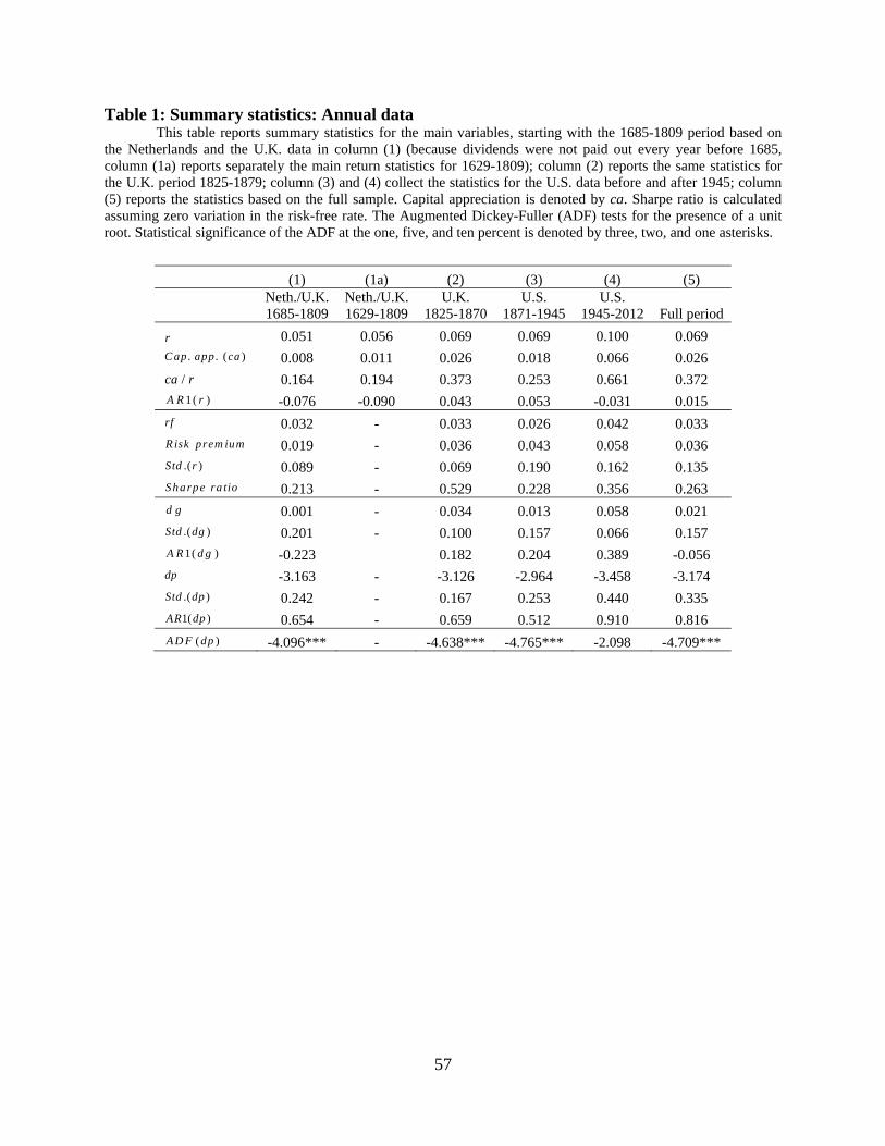
57

Table 1: Summary statistics: Annual data This table reports summary statistics for the main variables, starting with the 1685-1809 period based on the Netherlands and the U.K. data in column (1) (because dividends were not paid out every year before 1685, column (1a) reports separately the main return statistics for 1629-1809); column (2) reports the same statistics for the U.K. period 1825-1879; column (3) and (4) collect the statistics for the U.S. data before and after 1945; column (5) reports the statistics based on the full sample. Capital appreciation is denoted by ca. Sharpe ratio is calculated assuming zero variation in the risk-free rate. The Augmented Dickey-Fuller (ADF) tests for the presence of a unit root. Statistical significance of the ADF at the one, five, and ten percent is denoted by three, two, and one asterisks.

(1) (1a) (2) (3) (4) (5)

Neth./U.K. 1685-1809

Neth./U.K. 1629-1809

U.K. 1825-1870

U.S. 1871-1945

U.S. 1945-2012 Full period

r 0.051 0.056 0.069 0.069 0.100 0.069 . . ( )C ap app ca 0.008 0.011 0.026 0.018 0.066 0.026

/ca r 0.164 0.194 0.373 0.253 0.661 0.372 1( )A R r -0.076 -0.090 0.043 0.053 -0.031 0.015

rf 0.032 - 0.033 0.026 0.042 0.033 R isk prem ium 0.019 - 0.036 0.043 0.058 0.036

.( )Std r 0.089 - 0.069 0.190 0.162 0.135 Sharpe ra tio 0.213 - 0.529 0.228 0.356 0.263

d g 0.001 - 0.034 0.013 0.058 0.021 .( )Std dg 0.201 - 0.100 0.157 0.066 0.157 1( )A R d g -0.223 0.182 0.204 0.389 -0.056

dp -3.163 - -3.126 -2.964 -3.458 -3.174 .( )Std dp 0.242 - 0.167 0.253 0.440 0.335 1( )AR dp 0.654 - 0.659 0.512 0.910 0.816

( )A D F dp -4.096*** - -4.638*** -4.765*** -2.098 -4.709***

58

Table 1.A: Summary statistics: Triennial data This table reports summary statistics for the main variables, starting with the 1685-1809 period based on the Netherlands and the U.K. data in column (1) (because dividends were not paid out every year before 1685, column (1a) reports separately the main return statistics for 1629-1809); column (2) reports the same statistics for the U.K. period 1825-1879; column (3) and (4) collect the statistics for the U.S. data before and after 1945; column (5) reports the statistics based on the full sample. Capital appreciation is denoted by ca. Sharpe ratio is calculated assuming zero variation in the risk-free rate. The Augmented Dickey-Fuller (ADF) tests for the presence of a unit root. Statistical significance of the ADF at the one, five, and ten percent is denoted by three, two, and one asterisks.

(1) (1a) (2) (3) (4) (5)

Neth./U.K. 1685-1809

Neth./U.K. 1629-1809

U.K. 1825-1870

U.S. 1871-1945

U.S. 1945-2012 Full period

r 0.144 0.157 0.209 0.195 0.297 0.196 . . ( )C ap app ca 0.023 0.030 0.087 0.049 0.209 0.072

/ca r 0.161 0.190 0.415 0.250 0.705 0.369 .( )Std r 0.142 0.165 0.122 0.309 0.258 0.219 1( )A R r 0.012 0.113 -0.379 -0.342 0.031 -0.055

d g 0.015 0.031 0.104 0.030 0.157 0.062 .( )Std dg 0.145 0.446 0.149 0.245 0.106 0.344 1( )A R d g -0.128 -0.329 -0.367 -0.243 -0.140 -0.289

dp -2.071 -2.054 -2.051 -1.886 -2.460 -2.092 .( )Std dp 0.207 0.360 0.169 0.291 0.414 0.385 1( )AR dp 0.637 0.185 0.054 -0.085 0.707 0.442

59

Table 2: Vector autoregression (VAR) estimates: Annual data Panel A reports VAR estimates of returns, dividend growth rates, and the dividend-to-price ratio. The data is annual. The model is estimated by iterative generalized method of moments subject to the present value model constraints. Heteroskedasticity and autocorrelation corrected standard errors based on Bartlett kernel are reported in parentheses below the estimated parameters. The Newey and West method is used for the selection of the optimal bandwidth. In brackets we report a Chi-square statistic on the difference of a coefficient between a specific sub-period and the rest of the sample. Statistical significance at the one, five, and ten percent is denoted by three, two, and one asterisks. Panel B reports decomposition results based on the VAR estimates from Panel A.

(1) (2) (3) (4) (5)

Neth./U.K. 1685-1809

U.K. 1825-1870

U.S. 1871-1945

U.S. 1945-2012 Full period

Panel A: VAR estimates Dep. variable:

1tr

tdp 0.112*** 0.075 0.117 0.123*** 0.081***

(0.038) (0.046) (0.104) (0.036) (0.029) [3.311*] [0.512] [1.433] [0.677]

tr -0.055 0.071 0.144 -0.038 0.051

(0.078) (0.128) (0.208) (0.102) (0.079)

tdg 0.030 -0.099 -0.270** -0.095 -0.044

(0.077) (0.069) (0.117) (0.221) (0.056) Dep. variable:

1tdg

t

dp -0.187** -0.342*** -0.225*** 0.000 -0.123*** (0.086) (0.094) (0.059) (0.018) (0.030) [5.374**] [2.126] [0.213] [13.653***]

tr 0.019 -0.122 0.420*** 0.119 0.279***

(0.108) (0.261) (0.075) (0.081) (0.056)

tdg -0.035 0.255*** 0.135* 0.415*** 0.088

(0.113) (0.091) (0.075) (0.084) (0.099) Dep. variable:

1tdp

t

dp 0.730*** 0.609*** 0.692*** 0.904*** 0.830*** (0.098) (0.128) (0.102) (0.051) (0.043) [10.79***] [2.229] [2.089] [9.564***]

tr 0.077 -0.202 0.290 0.161 0.238**

(0.152) (0.358) (0.227) (0.158) (0.096)

tdg -0.067 0.370*** 0.425*** 0.526** 0.137

(0.123) (0.116) (0.150) (0.248) (0.120) J-test 2.674 0.399 1.806 1.391 8.702**

Panel B: Decomposition results Dividend-to-price DR 0.364 0.204 0.395 1.272 0.438 CF 0.636 0.796 0.605 -0.272 0.562 Unexpected returns DR 0.288 0.210 0.243 1.002 0.266 CF 0.713 0.791 0.762 -0.003 0.735

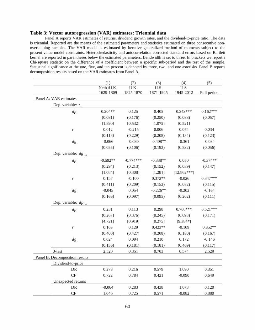
60

Table 3: Vector autoregression (VAR) estimates: Triennial data Panel A reports VAR estimates of returns, dividend growth rates, and the dividend-to-price ratio. The data is triennial. Reported are the means of the estimated parameters and statistics estimated on three consecutive non-overlapping samples. The VAR model is estimated by iterative generalized method of moments subject to the present value model constraints. Heteroskedasticity and autocorrelation corrected standard errors based on Bartlett kernel are reported in parentheses below the estimated parameters. Bandwidth is set to three. In brackets we report a Chi-square statistic on the difference of a coefficient between a specific sub-period and the rest of the sample. Statistical significance at the one, five, and ten percent is denoted by three, two, and one asterisks. Panel B reports decomposition results based on the VAR estimates from Panel A.

(1) (2) (3) (4) (5)

Neth./U.K. 1629-1809

U.K. 1825-1870

U.S. 1871-1945

U.S. 1945-2012 Full period

Panel A: VAR estimates Dep. variable:

1tr

tdp 0.204** 0.125 0.405 0.343*** 0.162***

(0.081) (0.176) (0.250) (0.088) (0.057) [1.890] [0.532] [1.075] [0.521]

tr 0.012 -0.215 0.006 0.074 0.034

(0.118) (0.229) (0.208) (0.134) (0.123)

tdg -0.066 -0.030 -0.408** -0.361 -0.034

(0.055) (0.106) (0.192) (0.532) (0.056) Dep. variable:

1tdg

t

dp -0.592** -0.774*** -0.338** 0.050 -0.374** (0.294) (0.213) (0.152) (0.039) (0.147) [1.084] [0.308] [1.281] [12.862***]

tr 0.157 -0.100 0.372** -0.026 0.347***

(0.411) (0.209) (0.152) (0.082) (0.115)

tdg -0.045 0.054 -0.226** -0.202 -0.164

(0.166) (0.097) (0.095) (0.202) (0.111) Dep. variable:

1tdp

t

dp 0.231 0.113 0.298 0.768*** 0.521*** (0.267) (0.376) (0.245) (0.093) (0.171) [4.721] [0.919] [0.275] [9.384*]

tr 0.163 0.129 0.423** -0.109 0.352**

(0.400) (0.427) (0.208) (0.180) (0.167)

tdg 0.024 0.094 0.210 0.172 -0.146

(0.156) (0.181) (0.181) (0.469) (0.117) J-test 2.520 0.351 0.703 0.574 2.529

Panel B: Decomposition results Dividend-to-price DR 0.278 0.216 0.579 1.090 0.351 CF 0.722 0.784 0.421 -0.090 0.649 Unexpected returns DR -0.064 0.283 0.438 1.073 0.120 CF 1.046 0.725 0.571 -0.082 0.880

61

Table 4: Longer horizon predictability This table reports return and dividend growth predictability results over different horizons. Panel A is based on overlapping observations, where the discounted sum of multi-year returns, multi-year dividend growth rates, and the future value of the dividend-to-price ratio are regressed on the lagged dividend-to-price ratio. Panel B reports the same results based on non-overlapping observations; we report the mean estimates across H different non-overlapping samples. The estimation is by iterative generalized method of moments subject to the present value model constraints. Heteroskedasticity and autocorrelation corrected standard errors based on a Bartlett kernel are reported in parentheses below the estimated parameters. Bandwidth is chosen optimally according to Newey-West method. Statistical significance at the one, five, and ten percent is denoted by three, two, and one asterisks. The period is from 1685 through 2012.

(1) (2) (3) Horizon (H) 1 year

1685-2012 3 years

1685-2012 5 years

1685-2012

Panel A: Overlapping observations

Dep. variable: 1

1

Hh

t hh

r

tdp 0.081*** 0.223*** 0.371***

(0.030) (0.065) (0.091)

Dep. variable: 1

1

Hh

t hh

dg

tdp -0.190*** -0.321*** -0.274***

(0.058) (0.094) (0.072)

Dep. variable: t Hdp

tdp 0.759*** 0.515*** 0.436***

(0.075) (0.140) (0.140)

J-test 1.273 2.249 2.533

Panel B: Non-overlapping observations

Dep. variable: 1

1

Hh

t hh

r

tdp 0.081*** 0.236*** 0.377***

(0.030) (0.084) (0.121)

Dep. variable: 1

1

Hh

t hh

dg

tdp -0.190*** -0.328*** -0.269**

(0.058) (0.114) (0.107)

Dep. variable: t Hdp

tdp 0.759*** 0.493*** 0.434**

(0.075) (0.173) (0.189)

J-test 1.273 1.828 1.935

62

Table 5: Cross-period out-of-sample predictions This table reports in-sample R-square and out-of-sample R-square (in brackets) for predicting annual returns and dividend growth rates. Both R-squares are calculated according to Eq. (16). The in-sample R-square is estimated over the same period as the estimated parameters. The out-of-sample R-square is calculated using estimated parameters from a different period; that is the out-of-sample R-square for the period 1685-1945 (1946-2012) is based on the estimated parameters from the period 1946-2012 (1685-1945). Results are based on the reduced form-model where returns and dividend growth rates are predicted using lagged dividend-to-price ratio only.

In-sample [out-of-sample] R-square 1685-1945 1945-2012

Returns Dividend growth

Returns Dividend growth

Parameters from: 1685-1945 0.034 0.205 [0.110] [-4.142] 1945-2012 [0.031] [-0.022] 0.115 0.011

63

Table 6: Predictability over the business cycle This table reports summary statistics (Panel A) and predictability results (Panel B) over the business cycle. Estimated parameters for expansions and recessions are estimated jointly using iterative generalized method of moments subject to the present value model constraints (Eq (17), (18)). Heteroskedasticity and autocorrelation corrected standard errors based on a Bartlett kernel are reported in parentheses below the estimated parameters. In brackets is the Wald test for equality of coefficients. Bandwidth is chosen optimally according to Newey-West method. Statistical significance at the one, five, and ten percent is denoted by three, two, and one asterisks. The period is either 1700-1945, or 1945-2012, or 1700-2012. (1) (2) (3) (4) (5) (6) 1700-1945 1945-2012 1700-2012

Recessions Expansions Recessions Expansions Recessions Expansions Panel A: Summary statistics r 0.027 0.087 -0.007 0.123 0.023 0.098 .( )S td r 0.140 0.111 0.215 0.140 0.148 0.121 t-stat [-3.576] *** [-2.006] * [-4.555] *** d g -0.005 0.025 0.033 0.063 -0.001 0.037 .( )S td d g 0.143 0.117 0.103 0.054 0.140 0.103 t-stat [-1.730] [-0.992] [-2.525] ** d p -3.066 -3.126 -3.270 -3.499 -3.087 -3.240 .( )S td d p 0.265 0.218 0.463 0.428 0.295 0.344 t-stat [1.855] [1.573] [4.106]*** No. of years 105 124 12 55 117 179

Panel B: VAR estimates

Dep. variable: 1tr

tdp 0.265*** 0.102*** 0.258*** 0.081* 0.117** 0.050

(0.082) (0.032) (0.069) (0.044) (0.052) (0.037) [3.375]* [4.699]** [1.104]

Dep. variable: 1tdg

tdp -0.174* -0.138*** 0.099* 0.003 -0.190** -0.079**

(0.089) (0.046) (0.055) (0.027) (0.076) (0.031) [0.123] [2.223] [1.800]

Dep. variable: 1tdp

tdp 0.587*** 0.795*** 0.870*** 0.951*** 0.723*** 0.906***

(0.098) (0.056) (0.109) (0.054) (0.085) (0.059) [3.369]* [0.436] [3.129]*

J-test 10.507** 0.084 0.948

64

Table 7: The effect of stock market duration: Simulations This table reports summary statistics (Panel A) and predictability results (Panel B) for simulated data based on our model for a market with finitely lived companies. Each company lives for years. The rest of parameters are taken from Binsbergen and Koijen (2010) (Table VI, p. 1463). We let simulations run for 10,000 years. The details are provided in Appendix B.

(1) (2) (3) 100 40 10

Panel A: Summary statistics r 0.091 0.090 0.091 . .C ap app 0.048 0.019 -0.130 dp -3.152 -2.627 -1.403

Panel B: VAR results Dep. variable:

1tr

tdp 0.123 0.148 0.214

Dep. variable:

1tdg

t

dp -0.000 -0.010 -0.156 Dep. variable:

1tdp

t

dp 0.914 0.902 0.785

Panel C: Decomposition of the dividend-to price DR 0.999 0.935 0.578 CF 0.001 0.065 0.422

65

Figure 1: Returns, dividend growth rates, and the dividend-to-price ratio This figure plots returns, dividend growth rates, and the dividend-to-price ratio. The data is annual. Vertical dashed lines denote the time periods: Netherlands and U.K. (1685-1809), U.K. (1825-1879), U.S. pre-war (1871-1945), and U.S. post-war (1945-2012). Panel A: Annual returns

Panel B: Annual dividend growth rates

Panel C: Dividend-to-price ratio

1705 1745 1785 1825 1865 1905 1945 1985

-0.4

-0.2

0

0.2

0.4

0.6

1705 1745 1785 1825 1865 1905 1945 1985-0.8

-0.6

-0.4

-0.2

0

0.2

0.4

0.6

1705 1745 1785 1825 1865 1905 1945 1985-4.5

-4

-3.5

-3

-2.5

-2

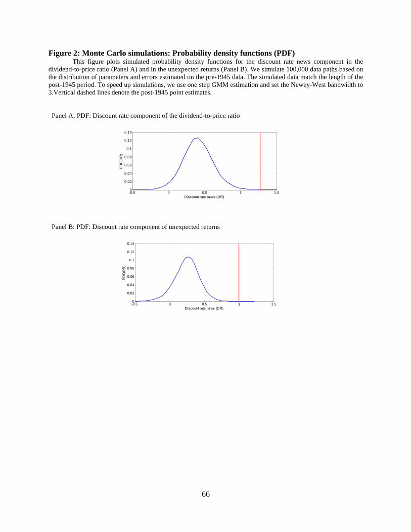
66

Figure 2: Monte Carlo simulations: Probability density functions (PDF) This figure plots simulated probability density functions for the discount rate news component in the dividend-to-price ratio (Panel A) and in the unexpected returns (Panel B). We simulate 100,000 data paths based on the distribution of parameters and errors estimated on the pre-1945 data. The simulated data match the length of the post-1945 period. To speed up simulations, we use one step GMM estimation and set the Newey-West bandwidth to 3.Vertical dashed lines denote the post-1945 point estimates.

Panel A: PDF: Discount rate component of the dividend-to-price ratio

Panel B: PDF: Discount rate component of unexpected returns

-0.5 0 0.5 1 1.50

0.02

0.04

0.06

0.08

0.1

0.12

0.14

Discount rate news (DR)

PD

F(D

R)

-0.5 0 0.5 1 1.50

0.02

0.04

0.06

0.08

0.1

0.12

0.14

Discount rate news (DR)

PD

F(D

R)

67

Figure 3: Dividends-to-earnings ratio This figure plots 20 year rolling averages of the dividends-to-earnings ratio for the Netherlands/U.K. (1685-1809) period and the combined U.S. period (1871-2012).

1678 1698 1718 1738 1758 1778 17980.2

0.4

0.6

0.8

1

1.2

1.4

1.6Netherlands/U.K.

1898 1918 1938 1958 1978 19980.2

0.4

0.6

0.8

1

1.2

1.4

1.6U.S.

68

Figure 4: Duration and discount rates: Rolling windows This figure plots our measure of duration along with either the discount rate component of the dividend-to-price ratio (Panel A) or the discount rate component of unexpected returns (Panel B). All measures are estimated on rolling windows of 68 years (to match the length of the post-1945 period). Estimations are done separately for the Netherlands/U.K. (1685-1809) period and the combined U.S. period (1871-2012). The first rolling window ends in 1753 for the Netherlands/U.K. and in 1939 for the U.S. period. Panel A: Duration and discount rate component of the dividend-to-price ratio

Panel B: Duration and discount rate component of unexpected returns

1761 1771 1781 1791 1801

0.2

0.4

0.6

0.8

1

1.2

1.4

1.6

Netherlands/U.K.

DR newsDuration

1947 1957 1967 1977 1987 1997 2007

0.2

0.4

0.6

0.8

1

1.2

1.4

1.6

U.S.

DR newsDuration

1761 1771 1781 1791 1801

0.2

0.4

0.6

0.8

1

1.2

1.4

1.6

Netherlands/U.K.

DR newsDuration

1947 1957 1967 1977 1987 1997 2007

0.2

0.4

0.6

0.8

1

1.2

1.4

1.6

U.S.

DR newsDuration

69

Figure 5: Duration, dividend smoothing parameter, and discount rates: Rolling windows (U.S. period: 1871-2012) This figure plots our measure of duration along with the dividend smoothing parameter and either the discount rate component of the dividend-to-price ratio (Panel A) or the discount rate component of unexpected returns (Panel B). Dividend smoothing parameter is a ratio of dividend growth volatility and the earnings growth volatility. All measures are estimated on the annual U.S. data from 1871 through 20012 using rolling windows of 68 years (to match the length of the post-1945 period). The first rolling window ends in 1939. Panel A: Duration, dividend smoothing parameter, and discount rate component of the dividend-to-price ratio

Panel B: Duration, dividend smoothing parameter, and discount rate component of unexpected returns

1940 1950 1960 1970 1980 1990 2000 2010

0.2

0.4

0.6

0.8

1

1.2

1.4

1.6

DR newsDurationSmoothing

1940 1950 1960 1970 1980 1990 2000 2010

0.2

0.4

0.6

0.8

1

1.2

1.4

1.6

DR newsDurationSmoothing

70

Online Appendix A: Reduced-form model

We repeat all our main results from Table 2 using a reduced form model. In particular,

rather than using the full VAR model, we predict returns, dividend growth rates, and the

dividend-to-price ratio by the lagged values of the dividend-to-price ratio only (as before, all

variables are demeaned):

1 1

1 1

1 1

,

,

,

r rt t t

dg dgt t t

dp dpt t t

r dp

dg dp

dp dp

(OA 1)

subject to the constraint imposed by the present value model:

1.r dg dp (OA 2)

We have three moment conditions and one linear restriction. As in the main analysis, we

estimate the system of equation by iterative GMM and report heteroscedasticity and

autocorrelation consistent statistics.

Based on the estimated parameters, we infer long-horizon estimates from their short-run

analogs. Dividing Eq. (OA 2) by 1 dp and rearranging, we obtain:

11 1

r dg

dp dp

(OA 3)

The first term can be interpreted as the variation of the dividend-to-price ratio due to discount

rates. Negative the second term captures variation due to cash-flows (see also Cochrane 2008).

Results are reported in Table OA 1 and are very similar to the results from the main

analysis reported in Table 2.

71

Table OA.1: Reduced-form model: Annual data Panel A reports the regression estimates of returns, dividend growth rates, and the dividend-to-price ratio on the lagged dividend-to-price ratio. The data are annual. The model is estimated by iterative generalized method of moments subject to the present value model constraint. Heteroskedasticity and autocorrelation corrected standard errors based on Bartlett kernel are reported in parentheses below the estimated parameters. The Newey and West method is used for the selection of the optimal bandwidth. Statistical significance at the one, five, and ten percent is denoted by three, two, and one asterisks. Panel B reports decomposition results based on the parameter estimates from Panel A.

(1) (2) (3) (4) (5)

Neth./U.K. 1685-1809

U.K. 1825-1870

U.S. 1871-1945

U.S. 1945-2012 Full period

Panel A: VAR estimates Dep. variable:

1tr

tdp 0.120*** 0.063** 0.055 0.123*** 0.081***

(0.034) (0.026) (0.073) (0.044) (0.030) Dep. variable:

1tdg

t

dp -0.230*** -0.294*** -0.450*** 0.015 -0.190*** (0.088) (0.046) (0.068) (0.025) (0.058) Dep. variable:

1tdp

t

dp 0.677*** 0.671*** 0.520*** 0.920*** 0.759*** (0.100) (0.045) (0.091) (0.048) (0.075) J-test 2.290 0.003 0.201 0.104 1.273

Panel B: Decomposition results Dividend-to-price DR 0.342 0.175 0.109 1.139 0.300 CF 0.658 0.825 0.891 -0.139 0.700

72

Online Appendix B: Inflation adjustment

In this Appendix, we repeat our main results from Table 2 using inflation adjusted prices

and dividends. The data for the earlier period come from the website of the International Institute

of Social History (http://www.iisg.nl/hpw/data.php#netherlands) (The Netherlands between 1629

and 1809) and Clark (2015) (England between 1825 and 1870). For the U.S. period, we use the

inflation index (CPI) from Robert Shiller’s webpage.

Note that the sub-periods differ substantially in terms of inflation. In the early periods,

inflation was relatively modest. Prices increased by 45% in the Netherlands/U.K. period 1685-

1809. In the U.K. period 1825-1870 prices decreased by 22.5%. In the early part of the U.S.

sample 1871-1945, prices increased again by 44%. In sharp contrast to the early samples,

inflation in the post-1945 period was substantially higher; the CPI increased 12.6 times, which

corresponds to 3.91% per year, on average.

These large differences in inflation, however, cannot account for the increase in the

discount rate news in the recent period. As reported in Table OA.2, the results for inflation

adjusted data are very comparable to the main results in Table 2. The only notable difference is

that returns become somewhat more predictable and dividend growth rates somewhat less

predictable in the early periods. The contrast between the recent U.S. period and the early

periods, however, remains.

73

Table OA 2: Vector autoregression (VAR) estimates: Annual inflation adjusted data Panel A reports VAR estimates of returns, dividend growth rates, and the dividend-to-price ratio. The data is annual and adjusted for inflation. The model is estimated by iterative generalized method of moments subject to the present value model constraints. Heteroskedasticity and autocorrelation corrected standard errors based on Bartlett kernel are reported in parentheses below the estimated parameters. The Newey and West method is used for the selection of the optimal bandwidth. Statistical significance at the one, five, and ten percent is denoted by three, two, and one asterisks. Panel B reports decomposition results based on the VAR estimates from Panel A.

(1) (2) (3) (4) (5)

Neth./U.K. 1685-1809

U.K. 1825-1870

U.S. 1871-1945

U.S. 1945-2012 Full period

Panel A: VAR estimates Dep. variable:

1tr

tdp 0.136*** 0.244** 0.138 0.118*** 0.108***

(0.042) (0.107) (0.088) (0.037) (0.029)

tr -0.002 0.180* 0.115 -0.027 0.032

(0.079) (0.105) (0.169) (0.094) (0.060)

tdg 0.003 -0.003 -0.261* 0.099 0.021

(0.085) (0.119) (0.145) (0.194) (0.072) Dep. variable:

1tdg

t

dp -0.145 -0.209* -0.282*** -0.007 -0.068** (0.090) (0.110) (0.074) (0.020) (0.030)

tr 0.158 -0.194 0.272** 0.124* 0.175**

(0.107) (0.199) (0.102) (0.069) (0.066)

tdg -0.050 0.291** 0.047 0.307*** 0.027

(0.092) (0.122) (0.089) (0.079) (0.090) Dep. variable:

1tdp

t

dp 0.749*** 0.571*** 0.610*** 0.902*** 0.858*** (0.108) (0.104) (0.100) (0.050) (0.047)

tr 0.167 -0.391** 0.165 0.155 0.149

(0.119) (0.189) (0.214) (0.134) (0.092)

tdg -0.055 0.307** 0.323* 0.215 0.007

(0.100) (0.140) (0.168) (0.185) (0.099) J-test 2.360 0.054 1.804 1.105 6.752*

Panel B: Decomposition results Dividend-to-price DR 0.524 0.482 0.411 1.084 0.672 CF 0.476 0.518 0.589 -0.084 0.328 Unexpected returns DR 0.241 0.254 0.312 0.839 0.447 CF 0.761 0.746 0.694 0.161 0.555