Foundations of Chemical Kinetics

Lecture 12: Transition-state theory: Thethermodynamic formalism

Marc R. Roussel

Department of Chemistry and Biochemistry

Breaking it down

I We can break down an elementary reaction into two steps:Reaching the transition state, and going through it into theproduct valley.

R TS→ P

I For a high barrier, there will be a Boltzmann distribution ofreactant energies which is only slightly disturbed by the leakacross the top of the barrier.

I This implies that we can treat the step R TS as being inequilibrium.

RK‡−−⇀↽−− TS

k‡−→ P

v = k‡[TS] (roughly)

Strategy

RK‡−−⇀↽−− TS

k‡−→ P

v = k‡[TS]

I This is an elementary reaction (R→ P), so its rate ought tobe v = k[R].

I We will use the equilibrium condition to eliminate [TS].This will bring thermodynamic quantities related to theequilibrium constant into the theory.

I We will use a quantum-statistical argument to get a value forthe specific rate of crossing of the barrier k‡.

Review of some elementary thermodynamicsFree energy

I The Gibbs free energy (G ) is defined by

G = H − TS

H: enthalpy (∆H = heat at const. p)S : entropy (measure of energy dispersal)

I The Gibbs free energy change is the maximum non-pV workavailable from a system.

Review of some elementary thermodynamicsFree energy (continued)

I For a reaction bB + cC→ dD + eE, the Gibbs free energychange is

∆rGm = ∆rG◦m + RT lnQ

where ∆rG◦m is the free energy change under standard

conditions:

∆rG◦m = d∆f G

◦(D) + e∆f G◦(E)− [b∆f G

◦(B) + c∆f G◦(C)]

I The reaction quotient Q is defined as

Q =adD aeEabB acC

where ai is the activity of species i .

Review of some elementary thermodynamicsActivity

I The activity also depends on the definition of the standardconditions:

In the gas phase, ai = γipi/p◦ where p◦ is the standard

pressure (usually 1 bar).For a solute, ai = γici/c

◦ where c◦ is the standardconcentration.There are several different conventions used forstandard concentrations, the most commonbeing 1 mol/kg and 1 mol/L.

γi is the activity coefficient (sometimes known as afugacity coefficient in the gas phase) of species i ,a measure of the deviation from ideal behavior.γi = 1 for an ideal substance.

Review of some elementary thermodynamicsEquilibrium

I At equilibrium, ∆rGm = 0, i.e.

∆rG◦m = −RT lnK

where K is the numerical constant such that Q = K atequilibrium.

I This equation can be rewritten

K = exp

(−∆rG

◦m

RT

).

Note that K is related to ∆rG◦m, the standard free energy

change.

Correction:Statistical equilibrium constant in a general reaction

Reaction: aA + bB cC + dDCorrect equation:

K =Qc

CQdD

QaAQ

bB

N−∆n exp

(−∆E0

kBT

)

I ∆n = c +d − (a+b) (difference of stoichiometric coefficients)

I N is the number of molecules (dimensionless).

I The translational partition function depends on V .N and V are chosen to be consistent with the standard state.

Example: For p◦ = 1 bar at 25 ◦C, p/RT = 40.34 mol m−3,so we could pick V = 1 m3 andN = 40.34× 6.022× 1023 = 2.429× 1025.

The K ‡ equilibriumCase 1: First-order elementary reaction

I We are treating the “equilibrium”

RK‡−−⇀↽−− TS

I For this equilibrium,

K ‡ =aTS

aR=⇒ aTS = K ‡aR

I If we assume ideal behavior or similar activity coefficients forR and TS, we get

[TS] = K ‡[R]

∴ v = k‡K ‡[R]

∴ k = k‡K ‡

The K ‡ equilibriumCase 2: Second-order elementary reaction

I The equilibrium is

X + YK‡−−⇀↽−− TS

I Now,

K ‡ =aTS

aX aY=⇒ aTS = K ‡aX aY

I Since ai = γici/c◦, this becomes

[TS] =K ‡

c◦γXγY

γTS[X][Y]

I Assuming ideal behavior, we get

[TS] =K ‡

c◦[X][Y]

which gives

k =k‡K ‡

c◦

The K ‡ equilibriumFirst- vs second-order rate constants

I Since the difference between the first- and second-order casesis just a factor of c◦, we treat the second-order case from hereon.

Mathematical interlude: Taylor series

I For any “nice” function,

f (x) ≈ f (a)+f ′(a)(x−a)+f ′′(a)

2(x−a)2+. . .+

f (n)(a)

n!(x−a)n

I For small x , take a = 0:

f (x) ≈ f (0) + f ′(0)x +1

2f ′′(0)x2 + . . .

I In practice we often stop at the first non-trivial term (i.e. thefirst term after f (0) that isn’t identically zero).

Units of frequency

I In our treatment of vibration, we have so far used the angularfrequency ω, whose units can be thought of as rad s−1.

I We can also express frequencies in Hz, i.e. cycles per second,typically denoted ν.

I Since ω = 2πν and ~ = h/2π, ~ω = hν.

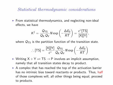
Statistical thermodynamic considerations

I From statistical thermodynamics, and neglecting non-idealeffects, we have

K ‡ =QTS

QX QYN exp

(−∆E0

RT

)=

c◦[TS]

[X][Y],

where QTS is the partition function of the transition state.

∴ [TS] =[X][Y]

c◦QTS

QX QYN exp

(−∆E0

RT

)I Writing X + Y TS→ P involves an implicit assumption,

namely that all transition states decay to product.

I A complex that has reached the top of the activation barrierhas no intrinsic bias toward reactants or products. Thus, halfof those complexes will, all other things being equal, proceedto products.

Statistical thermodynamic considerations(continued)

I Define the concentration of transition states leading toproduct formation as

[TS→P] =1

2[TS] =

1

2

[X][Y]

c◦QTS

QX QYN exp

(−∆E0

RT

)I The reaction rate is therefore correctly cast as

v = k‡[TS→P] =1

2k‡

[X][Y]

c◦QTS

QX QYN exp

(−∆E0

RT

)which gives

k =1

2

k‡

c◦QTS

QX QYN exp

(−∆E0

RT

)

Statistical thermodynamic considerations(continued)

I We assume that the transition-state partition function factors,i.e. that motion along the reactive normal mode isindependent of other molecular motions:

QTS = Q‡Qr

where Qr is the part of the partition function associated withthe reactive normal mode (i.e. the motion through the saddle)while Q‡ is the rest of the partition function.

Statistical thermodynamic considerations(continued)

I Assume we can treat the reactive mode as a vibration, withpartition function

Qr = [1− exp(−hνr/kBT )]−1

I Since the reactive mode is “loose”, assume hνr/kBT is small.

I Taylor expansion for small x :

1− e−x ≈ x

∴(1− e−x

)−1 ≈ x−1

∴ Qr ≈kBT

hνr

Statistical thermodynamic considerations(continued)

I The rate constant becomes

k =1

2

k‡

c◦kBT

hνr

Q‡

QX QYN exp

(−∆E0

RT

)I νr represents the frequency for a full “vibrational” cycle of the

reactive mode (back and forth).

I k‡ is the frequency for crossing the saddle in one directiononly.

∴ k‡ = 2νr

∴ k =kBT

c◦h

Q‡

QX QYN exp

(−∆E0

RT

)

Statistical formula for the rate constantInterpretation

k =kBT

c◦h

Q‡

QX QYN exp

(−∆E0

RT

)I Q‡ is the partition function for the transition state omitting

the reactive mode.

I ∆E0 is the difference in zero point energies between thereactants and transition state.

I Q‡

QX QYN exp

(−∆E0

RT

)is of the form of an equilibrium constant

with one mode (the reactive mode) removed.

Statistical formula for the rate constantApplication

k =kBT

c◦h

Q‡

QX QYN exp

(−∆E0

RT

)In principle, we can use this equation to compute rate constants.In practice, this isn’t so easy because:

I We need to know the geometry of the transition state.

I We need to know the height of the barrier and zero-pointenergies of the reactants and transition state.

I We need to know the vibrational spectrum of the transitionstate.

All of this information is in principle available either from verygood quantum chemical calculations or from transition-statespectroscopy.

Thermodynamic interpretation

k =kBT

c◦h

Q‡

QX QYN exp

(−∆E0

RT

)I Define

K ‡ =Q‡

QX QYN exp

(−∆E0

RT

)I Note that this isn’t quite a normal equilibrium constant

because we have removed one mode from the transition statepartition function.

I We can still write

K ‡ = exp

(−∆‡G ◦m

RT

)

Thermodynamic interpretation(continued)

k =kBT

c◦hexp

(−∆‡G ◦m

RT

)∴ k =

kBT

c◦hexp

(∆‡S◦mR

)exp

(−∆‡H◦m

RT

)

Relationship to Arrhenius parameters

From ln k = lnA− Ea/RT , we have

d ln k

dT= Ea/RT

2

or

Ea = RT 2 d ln k

dT.

Relationship to Arrhenius parameters(continued)

I For the transition-state theory expression,

ln k = ln

(kBT

c◦h

)+

∆‡S◦mR− ∆‡H◦m

RT

∂ ln k

∂T

∣∣∣∣p

=1

T+

1

R

∂∆‡S◦m∂T

∣∣∣∣p

− 1

RT

∂∆‡H◦m∂T

∣∣∣∣p

+∆‡H◦mRT 2

Relationship to Arrhenius parameters(continued)

I There is some cancellation of terms, and a few furtherassumptions based on typical values of thermodynamicquantities. We eventually get

∂ ln k

∂T

∣∣∣∣p

=1

T+

∆‡H◦mRT 2

− ∆‡ngas

T

where ∆‡ngas is the dimensionless change in the number ofequivalents of gas on going from the reactants to thetransition state (zero for a unimolecular reaction, −1 for abimolecular reaction).

Relationship to Arrhenius parameters(continued)

I Thus,

Ea = RT 2 d ln k

dT

∴ Ea = ∆‡H◦m + RT(

1−∆‡ngas)

I If we solve for ∆‡H◦m in terms of Ea, put the result back intoour TST rate constant expression and rearrange, we get

k =kBT

c◦hexp

(∆‡S◦mR

)exp(1−∆‡ngas) exp

(− Ea

RT

)I By comparison to the Arrhenius equation, we get

A =kBT

c◦hexp

(∆‡S◦mR

)exp(1−∆‡ngas)

Eyring plot

I Go back to the thermodynamic TST equation:

k =kBT

c◦hexp

(∆‡S◦mR

)exp

(−∆‡H◦m

RT

)∴ ln

(kc◦h

kBT

)=

∆‡S◦mR− ∆‡H◦m

RT

I Plotting ln(kc◦h/kBT ) vs T−1 should give a straight line ofslope −∆‡H◦m/R and intercept ∆‡S◦m/R.