Embed Size (px)
Citation preview
Forward Rasterization
VOICU POPESCU and PAUL ROSEN
Purdue University
We describe forward rasterization, a class of rendering algorithms designed for small polygonal primitives. The primitive is
efficiently rasterized by interpolation between its vertices. The interpolation factors are chosen to guarantee that each pixel
covered by the primitive receives at least one sample which avoids holes. The location of the samples is recorded with subpixel
accuracy using a pair of offsets which are then used to reconstruct/resample the output image. Offset reconstruction has good
static and temporal antialiasing properties. We present two forward rasterization algorithms, one that renders quadrilaterals
and is suitable for scenes modeled with depth images like in image-based rendering by 3D warping, and one that renders triangles
and is suitable for scenes modeled conventionally. When compared to conventional rasterization, forward rasterization is more
efficient for small primitives and has better temporal antialiasing properties.
Categories and Subject Descriptors: I.3.3 [Computer Graphics]: Picture/Image Generation—Display algorithms
General Terms: Theory, Performance
Additional Key Words and Phrases: 3D warping, point-based modeling and rendering, rendering pipeline, rasterization,
antialiasing
1. INTRODUCTION
In raster graphics, rendering algorithms take as input a scene description and a desired view andproduce an image by computing the color of each pixel on a 2D grid. In order to compute the color at agiven pixel, the traditional approach is to establish an inverse mapping from the image plane to the sceneprimitives (from output to input). The ray tracing pipeline potentially computes an inverse mappingfrom every pixel to every scene primitive. The method is inefficient since only a few pixel/primitivepairs yield a color sample. In spite of acceleration schemes that consider only plausible pixel/primitivepairs, ray tracing is not the method of choice in interactive rendering.
Most interactive graphics applications rely on the feed-forward pipeline. The primitives are firstforward mapped to the image plane by vertex projection. Then an inverse mapping from the image tothe primitive is computed at rasterization setup. The mapping is used during rasterization to fill in thepixels covered by the primitive. This approach is efficient for primitives with sizeable image projections:the rasterization setup cost is amortized over a large number of interior pixels.
For small primitives, like the ones encountered in complex scenes or in image-based rendering (IBR),the approach is inefficient since the inverse mapping is used for only a few pixels. Researchers in IBR
This research was supported by NSF, DARPA, and the Computer Science Departments of the University of North Carolina at
Chapel Hill and of Purdue University.
Authors’ address: Computer Sciences Department, Purdue University, 250 N University Street, West Lafayette IN 47907-2066;
email: [email protected] and [email protected].
Permission to make digital or hard copies of part or all of this work for personal or classroom use is granted without fee provided
that copies are not made or distributed for profit or direct commercial advantage and that copies show this notice on the first
page or initial screen of a display along with the full citation. Copyrights for components of this work owned by others than ACM
must be honored. Abstracting with credit is permitted. To copy otherwise, to republish, to post on servers, to redistribute to lists,
or to use any component of this work in other works requires prior specific permission and/or a fee. Permissions may be requested
from Publications Dept., ACM, Inc., 1515 Broadway, New York, NY 10036 USA, fax: +1 (212) 869-0481, or [email protected].
c© 2006 ACM 0730-0301/06/0400-0375 $5.00
ACM Transactions on Graphics, Vol. 25, No. 2, April 2006, Pages 375–411.
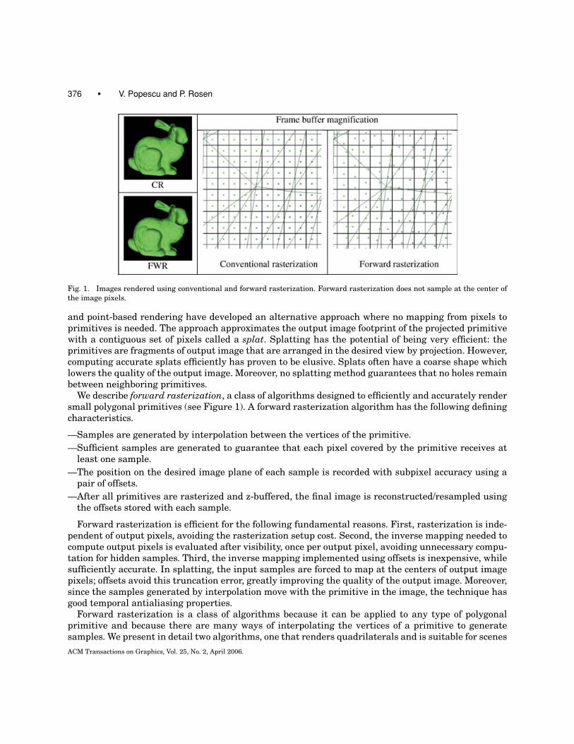
376 • V. Popescu and P. Rosen
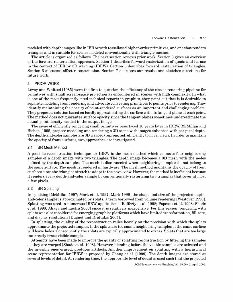
Fig. 1. Images rendered using conventional and forward rasterization. Forward rasterization does not sample at the center of
the image pixels.
and point-based rendering have developed an alternative approach where no mapping from pixels toprimitives is needed. The approach approximates the output image footprint of the projected primitivewith a contiguous set of pixels called a splat. Splatting has the potential of being very efficient: theprimitives are fragments of output image that are arranged in the desired view by projection. However,computing accurate splats efficiently has proven to be elusive. Splats often have a coarse shape whichlowers the quality of the output image. Moreover, no splatting method guarantees that no holes remainbetween neighboring primitives.
We describe forward rasterization, a class of algorithms designed to efficiently and accurately rendersmall polygonal primitives (see Figure 1). A forward rasterization algorithm has the following definingcharacteristics.
—Samples are generated by interpolation between the vertices of the primitive.
—Sufficient samples are generated to guarantee that each pixel covered by the primitive receives atleast one sample.
—The position on the desired image plane of each sample is recorded with subpixel accuracy using apair of offsets.
—After all primitives are rasterized and z-buffered, the final image is reconstructed/resampled usingthe offsets stored with each sample.
Forward rasterization is efficient for the following fundamental reasons. First, rasterization is inde-pendent of output pixels, avoiding the rasterization setup cost. Second, the inverse mapping needed tocompute output pixels is evaluated after visibility, once per output pixel, avoiding unnecessary compu-tation for hidden samples. Third, the inverse mapping implemented using offsets is inexpensive, whilesufficiently accurate. In splatting, the input samples are forced to map at the centers of output imagepixels; offsets avoid this truncation error, greatly improving the quality of the output image. Moreover,since the samples generated by interpolation move with the primitive in the image, the technique hasgood temporal antialiasing properties.
Forward rasterization is a class of algorithms because it can be applied to any type of polygonalprimitive and because there are many ways of interpolating the vertices of a primitive to generatesamples. We present in detail two algorithms, one that renders quadrilaterals and is suitable for scenes
ACM Transactions on Graphics, Vol. 25, No. 2, April 2006.
Forward Rasterization • 377
modeled with depth images like in IBR or with tessellated higher-order primitives, and one that renderstriangles and is suitable for scenes modeled conventionally with triangle meshes.
The article is organized as follows. The next section reviews prior work. Section 3 gives an overviewof the forward rasterization approach. Section 4 describes forward rasterization of quads and its usein the context of IBR by 3D warping (IBRW). Section 5 describes forward rasterization of triangles.Section 6 discusses offset reconstruction. Section 7 discusses our results and sketches directions forfuture work.
2. PRIOR WORK
Levoy and Whitted [1985] were the first to question the efficiency of the classic rendering pipeline forprimitives with small screen-space projection as encountered in scenes with high complexity. In whatis one of the most frequently cited technical reports in graphics, they point out that it is desirable toseparate modeling from rendering and advocate converting primitives to points prior to rendering. Theyidentify maintaining the opacity of point-rendered surfaces as an important and challenging problem.They propose a solution based on locally approximating the surface with its tangent plane at each point.The method does not guarantee surface opacity since the tangent planes sometimes underestimate theactual point density needed in the output image.
The issue of efficiently rendering small primitives resurfaced 10 years later in IBRW. McMillan andBishop [1995] propose modeling and rendering a 3D scene with images enhanced with per pixel depth.The depth-and-color samples are 3D warped (reprojected) efficiently to novel views. In order to maintainthe opacity of front surfaces, two approaches are investigated.
2.1 IBR Mesh Method
A possible reconstruction technique for IBRW is the mesh method which connects four neighboringsamples of a depth image with two triangles. The depth image becomes a 3D mesh with the nodesdefined by the depth samples. The mesh is disconnected when neighboring samples do not belong tothe same surface. The mesh is rendered in hardware. The mesh method maintains the opacity of frontsurfaces since the triangles stretch to adapt to the novel view. However, the method is inefficient becauseit renders every depth-and-color sample by conventionally rasterizing two triangles that cover at mosta few pixels.
2.2 IBR Splatting
In splatting [McMillan 1997; Mark et al. 1997; Mark 1999] the shape and size of the projected depth-and-color sample is approximated by splats, a term borrowed from volume rendering [Westover 1990].Splatting was used in numerous IBRW applications [Rafferty et al. 1998; Popescu et al. 1998; Shadeet al. 1998; Aliaga and Lastra 2003] since it is relatively inexpensive. For this reason, rendering withsplats was also considered for emerging graphics platforms which have limited transformation, fill-rate,and display resolutions [Duguet and Drettakis 2004].
In splatting, the quality of the reconstruction relies heavily on the precision with which the splatsapproximate the projected samples. If the splats are too small, neighboring samples of the same surfacewill leave holes. Consequently, the splats are typically approximated to excess. Splats that are too largeincorrectly erase visible samples.
Attempts have been made to improve the quality of splatting reconstruction by filtering the samplesas they are warped [Shade et al. 1998]. However, blending before the visible samples are selected andthe invisible ones erased, produces artifacts. Another improvement on splatting with a hierarchicalscene representation for IBRW is proposed by Chang et al. [1999]. The depth images are stored atseveral levels of detail. At rendering time, the appropriate level of detail is used such that the projected
ACM Transactions on Graphics, Vol. 25, No. 2, April 2006.
378 • V. Popescu and P. Rosen
samples cover about one pixel of the desired image. Since splats are never bigger than one pixel, thereference images must always have at least the resolution of the desired view. The method suffers fromlengthy preprocessing times, large memory requirements, and reduced frame rates.
McAllister et al. [1999] used the programmable-primitives feature of PixelFlow [Molnar et al. 1992;Eyles et al. 1997] in order to reconstruct the warped image. Each sample is rasterized as a disk with aquadratic falloff in depth. This is similar to the technique of rendering Voronoi regions by rasterizingcones [Haeberli 1990] which was used before for reconstruction in image-based rendering [Larson 1998].The method relied on PixelFlow’s unique ability of efficiently rendering quadratics.
Researchers developed splatting techniques that produce high-quality images but that was onlyachieved by considerably increasing the complexity of the splats. The emphasis shifted from achievingefficient rendering to developing a versatile modeling paradigm.
2.3 Point-Based Graphics
The QSplat system [Rusinkiewicz and Levoy 2000] stores the scene as a hierarchy of bounding sphereswhich provides visibility-culling and level-of-detail adaptation during rendering. As with the previoussplatting methods, determining the shape and size of the splat is difficult. The system guarantees theopacity of the front surface if circular or square splats are used. However, coercing the splats to besymmetrical degrades the reconstruction. The authors report aliasing at the silhouette edges.
The surfel method [Pfister et al. 2000] is another variant of the splatting technique. Surfels are datastructures that contain sufficient information for reconstructing a fragment of a surface. Rendering withsurfels is done in two stages, visibility and then reconstruction. Visibility eliminates the hidden surfelsand is done by splatting model-space disks onto the desired-image plane and then scan-convertingtheir bounding parallelogram into the z-buffer. The cost of rendering a splat is that of rendering twotriangles. There is no guarantee that no holes remain. The output image is reconstructed from surfelsthat survive the visibility stage.
Elliptical Weighted Average (EWA) surface splatting [Zwicker et al. 2002; Ren et al. 2002] builds onthe surfels work to improve the quality of the reconstruction by adapting Heckbert’s work [1989] onfiltering irregular samples to point-based rendering. During a preprocessing stage, the points with colorare used to create a continuous texture which is used at run time to color the visible surface elements.The method enables high-quality anisotropic filtering within the surface and antialiases edges usingcoverage masks, bringing to point-based rendering what was previously possible only for polygonalrendering. However, porting these techniques to points comes at a higher cost since one has to overcomethe lack of connectivity and make do with approximate connectivity inferred from the distances to theneighboring samples. These techniques are readily available to IBRW when the reconstruction is basedon the triangle mesh approach which is the case of forward rasterization.
In recent work, Whitted and Kajiya [2005] investigate a programmable pipeline where geometryand shading are represented procedurally. The pipeline can be seen as a generalization of point-basedrendering. Programmable geometric primitives have been discussed before in the context of offline ren-dering [Whitted and Weimer 1982; Cook et al. 1987], and interactive rendering with special hardware[Olano 1998]. The novelty of the fully procedural pipeline is that the rasterizer is replaced with a sam-ple generator which generates samples until hole-free coverage is obtained. Samples are generated byKajiya invoking the geometric primitive procedure with different parameters. Forward rasterizationcan be seen as treating quads and triangles procedurally. Although Whitted and Kajiya’s and [2005]work is just a preliminary study with many aspects of the pipeline remaining to be refined, the workpoints out the potential advantage of forward rasterization, and it identifies which challenges have tobe overcome to concretize this advantage.
ACM Transactions on Graphics, Vol. 25, No. 2, April 2006.
Forward Rasterization • 379
2.4 Triangle Rasterization
Since this article proposes a forward rasterization for triangles, we also briefly review rasterizationand antialiasing approaches for polygonal rendering. Several techniques were proposed for filling inprojected triangles. An early technique referred to as Digital Differential Analyzer (DDA) walks on theedges of the triangle and splits the triangle in horizontal spans of pixels. The DDA approach is used bythe RealityEngine [Akeley 1993].
The Pixel-Planes architecture [Fuchs et al. 1985] has the ability to quickly evaluate linear expressionsfor many pixels in parallel and introduces the edge equations approach to rasterization. For a givenprojected triangle, edge equations and rasterization parameter planes are 2D linear expressions in thepixel coordinates (u, v). Given a pixel, deciding whether it is interior to the triangle and computing itsrasterization parameter values is done in a unified manner by evaluating 2D linear expressions. Whatremains is the question of which pixels to consider for a given triangle.
One approach is to use a rectangular screen-aligned bounding box. The advantage of the methodis its simplicity. Other approaches have been proposed. Pineda [1988] describes a traversal approachdriven by a center line. McCormack and McNamara [2000] describe traversal orders that generate allsamples belonging to one rectangular tile of the screen before proceeding to the next tile which is advan-tageous in the case of partitioned framebuffers. McCool et al. [2001] propose traversing the primitive’sbounding box on hierarchical Hilbert curves for improved spatial coherence. These methods reduce thenumber of exterior pixels considered but come at the price of increased per triangle and per scan-linecost.
InfiniteReality, the second SGI graphics supercomputer [Montrym et al. 1997], adopts the edge equa-tions approach to reduce the setup cost of DDA. PixelFlow [Molnar et al. 1992; Eyles et al. 1997], thesort-last successor of Pixel-Planes, continues to rasterize using linear expressions. In the mid nineties,the almost vertical progress of PC graphics accelerators begins. In a few years, add-in cards catch upfrom behind and render the graphics supercomputers obsolete [NVIDIA; ATI]. The specifics of the ar-chitectures and of the algorithms they implement are not published but a study of patent applicationsand whitepapers indicate that graphics cards use variants of the edge equation rasterization.
The graphics architecture literature describes several other rasterization approaches. Good overviewsof earlier variants of rasterization are given in the survey paper [Garachorloo et al. 1989], in Kaufman’sbook [1993], and in Ellsworth’s Ph.D. thesis [1996].
Greene [1996] describes a hierarchical rasterization (tiling) algorithm that integrates occlusionculling, rasterization, and antialiasing. The subpixel screen coverage of a triangle is determined re-cursively, using precomputed triage coverage masks for each of its 3 edges. Such a k × k mask storeswhich k × k subregions are inside, outside, or crossing the edge. The rasterization is essentially lookedup rather than computed. The method outperforms conventional software rasterization for static, high-depth complexity scenes. Dynamic scenes pose a problem since polygons cannot be presorted in front-to-back order, a requirement for efficient occlusion culling. The approach does not offer a viable stand-alonerasterization solution. The coverage masks avoid the computational cost of determining coverage, butreplace it with an increased bandwidth requirement to look up the masks. Moreover, the coveragecomputation is just a small fraction of the rasterization cost which is dominated by computing therasterization parameters at each pixel.
Homogeneous coordinates rasterization [Olano and Greer 1997] has the advantage of incorporatingclipping into rasterization which avoids the need of actually splitting the triangle. The triangle isenhanced with clip edges, one for each clip plane, including the planes defining the view frustum andany arbitrary clip planes specified by the application. The authors state that the algorithm requires ahigher number of operations because the hither clip edge requires interpolating all parameters with
ACM Transactions on Graphics, Vol. 25, No. 2, April 2006.
380 • V. Popescu and P. Rosen
perspective correction. Whether rasterization proceeds with homogeneous or projected coordinates isan issue orthogonal to the issue of forward versus inverse rasterization.
Barycentric rasterization [Brown 1999a, 1999b] is an algorithm that limits the setup computationsto establishing the linear expressions that give the variation of the barycentric coordinates in theimage plane. Then, for every pixel, the barycentric coordinates are used to decide whether the pixelis interior to the triangle, and, if it is, to blend the rasterization parameter values at the vertices. Inhis study of mapping the graphics pipeline to a programmable stream processor architecture, Owens[2003] proposes using barycentric rasterization to reduce the burden of carrying a large number ofinterpolants through the rasterization process. McCool et al. [2001] independently develop barycentricinterpolation (without explicitly calling it so) for the same purpose of better handling a large numberof interpolants.
There are numerous variants of inverse rasterization. We have chosen to compare forward rasteri-zation to the edge equation approach because it is widely adopted by hardware implementations andto barycentric rasterization because of its low setup cost.
2.5 Antialiasing
A fundamental challenge in raster graphics is dealing with the nonzero pixel size. The limited samplingrate limits the maximum frequency that can be displayed and ignoring this limit produces visuallydisturbing aliasing artifacts. Antialiasing techniques are expensive since they require rendering withsubpixel accuracy. Most techniques compute several color samples per pixel and then blend them toobtain the final pixel color. Stochastic sampling [Cook 1986] produces high quality images but is tooslow to be used in interactive graphics applications. See Glassner’s ray tracing book [1978] for a goodlist of additional references.
In interactive graphics, one approach is regular supersampling, where the pixel is subdivided in√
n ×√n subpixels. A better approach is to avoid collinear sampling locations. One possibility is random
sampling. Jittered supersampling perturbs the sampling locations away from the centers of the√
n ×√n subpixels. The n-rooks sampling pattern starts with an n × n subdivision of the pixel, selects one
sample randomly in each of the n cells of the main diagonal, and then shuffles the horizontal coordinateu of the samples. All these techniques, generically called jittered supersampling, employ samplinglocations that are defined with respect to the pixel grid and are, therefore, equivalent for the purposeof comparing forward to conventional rasterization. Molnar et al. [1991] investigates the number ofcolor samples per output pixel that is required to obtain high quality images. He concludes that goodresults are obtained with as little as 5 samples. The SAGE graphics architecture [Deering and Naegle2002] offers the option of up to 16 color samples per output pixel and complete flexibility regarding thereconstruction filter.
Carpenter [1984] introduces the a-buffer, a technique that achieves high-quality supersampling bystoring at each pixel a list of coverage masks. The algorithm is expensive, but it introduces the impor-tant idea that coverage computation is orthogonal to the number of color samples per pixel. Severalantialiasing algorithms were developed based on in this idea [Abram and Westover 1985; Schilling1991], and the idea is used in today’s (extended) graphics APIs [OpenGL, DirectX] which differenti-ate between multisampling and supersampling to imply higher resolution coverage or color sampling,respectively.
Antialiasing has a direct impact on quality so the antialiasing capability of a graphics card is aheavily marketed feature. Moreover, antialiasing always comes at a cost so application developers needto be provided with an understanding, albeit minimal, of the underlying algorithm in order to decidewhen to use it and with what parameters. For these reasons several whitepapers are available [NVIDIA2004, 2005a, 2005b] describing the antialiasing capabilities of graphics cards. A review of the various
ACM Transactions on Graphics, Vol. 25, No. 2, April 2006.
Forward Rasterization • 381
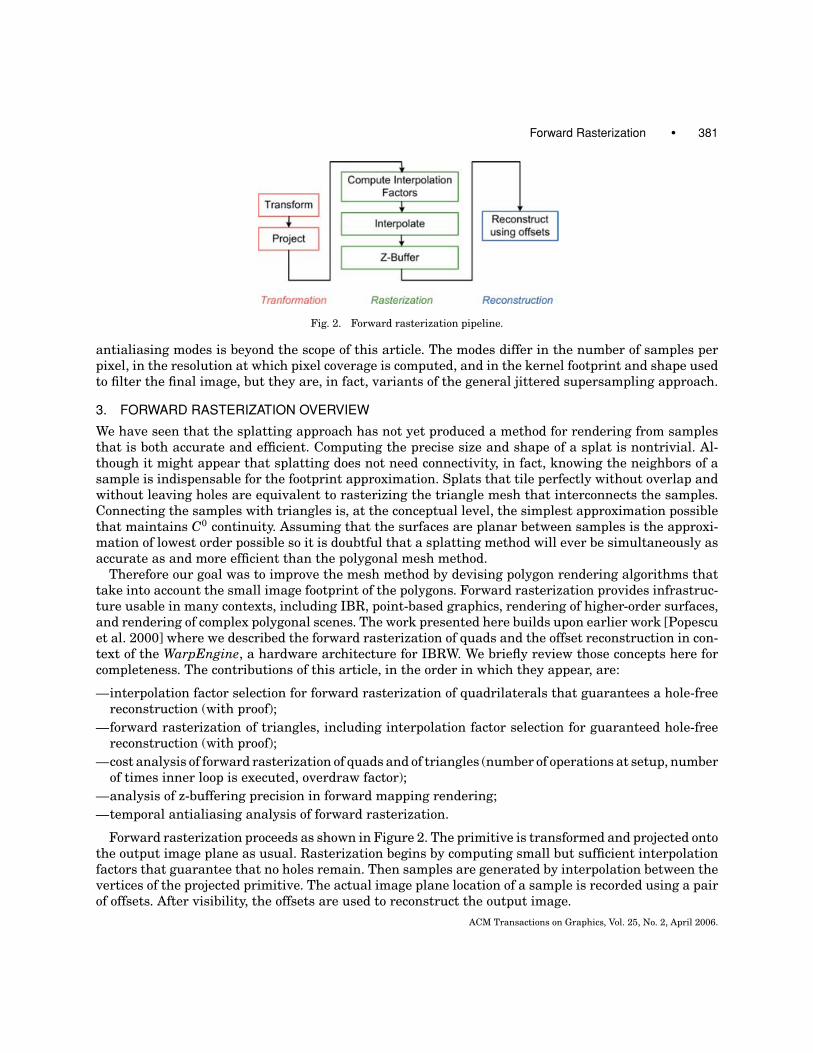
Fig. 2. Forward rasterization pipeline.
antialiasing modes is beyond the scope of this article. The modes differ in the number of samples perpixel, in the resolution at which pixel coverage is computed, and in the kernel footprint and shape usedto filter the final image, but they are, in fact, variants of the general jittered supersampling approach.
3. FORWARD RASTERIZATION OVERVIEW
We have seen that the splatting approach has not yet produced a method for rendering from samplesthat is both accurate and efficient. Computing the precise size and shape of a splat is nontrivial. Al-though it might appear that splatting does not need connectivity, in fact, knowing the neighbors of asample is indispensable for the footprint approximation. Splats that tile perfectly without overlap andwithout leaving holes are equivalent to rasterizing the triangle mesh that interconnects the samples.Connecting the samples with triangles is, at the conceptual level, the simplest approximation possiblethat maintains C0 continuity. Assuming that the surfaces are planar between samples is the approxi-mation of lowest order possible so it is doubtful that a splatting method will ever be simultaneously asaccurate as and more efficient than the polygonal mesh method.
Therefore our goal was to improve the mesh method by devising polygon rendering algorithms thattake into account the small image footprint of the polygons. Forward rasterization provides infrastruc-ture usable in many contexts, including IBR, point-based graphics, rendering of higher-order surfaces,and rendering of complex polygonal scenes. The work presented here builds upon earlier work [Popescuet al. 2000] where we described the forward rasterization of quads and the offset reconstruction in con-text of the WarpEngine, a hardware architecture for IBRW. We briefly review those concepts here forcompleteness. The contributions of this article, in the order in which they appear, are:
—interpolation factor selection for forward rasterization of quadrilaterals that guarantees a hole-freereconstruction (with proof);
—forward rasterization of triangles, including interpolation factor selection for guaranteed hole-freereconstruction (with proof);
—cost analysis of forward rasterization of quads and of triangles (number of operations at setup, numberof times inner loop is executed, overdraw factor);
—analysis of z-buffering precision in forward mapping rendering;
—temporal antialiasing analysis of forward rasterization.
Forward rasterization proceeds as shown in Figure 2. The primitive is transformed and projected ontothe output image plane as usual. Rasterization begins by computing small but sufficient interpolationfactors that guarantee that no holes remain. Then samples are generated by interpolation between thevertices of the projected primitive. The actual image plane location of a sample is recorded using a pairof offsets. After visibility, the offsets are used to reconstruct the output image.
ACM Transactions on Graphics, Vol. 25, No. 2, April 2006.
382 • V. Popescu and P. Rosen
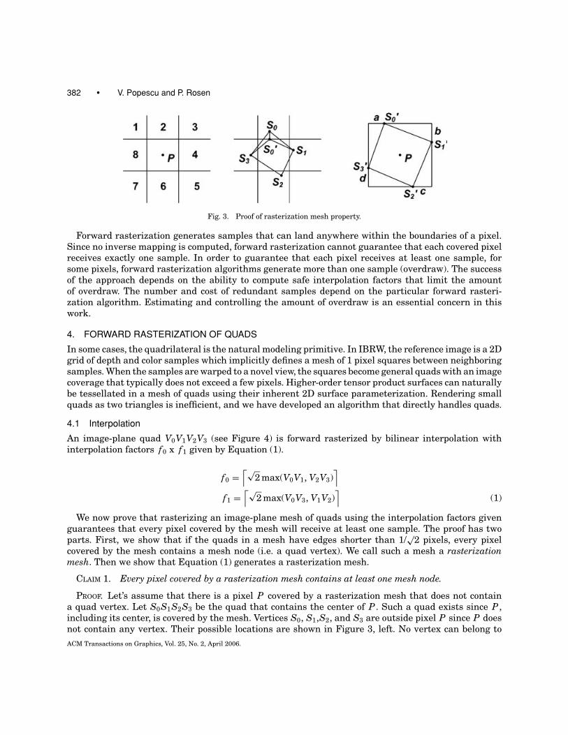
Fig. 3. Proof of rasterization mesh property.
Forward rasterization generates samples that can land anywhere within the boundaries of a pixel.Since no inverse mapping is computed, forward rasterization cannot guarantee that each covered pixelreceives exactly one sample. In order to guarantee that each pixel receives at least one sample, forsome pixels, forward rasterization algorithms generate more than one sample (overdraw). The successof the approach depends on the ability to compute safe interpolation factors that limit the amountof overdraw. The number and cost of redundant samples depend on the particular forward rasteri-zation algorithm. Estimating and controlling the amount of overdraw is an essential concern in thiswork.
4. FORWARD RASTERIZATION OF QUADS
In some cases, the quadrilateral is the natural modeling primitive. In IBRW, the reference image is a 2Dgrid of depth and color samples which implicitly defines a mesh of 1 pixel squares between neighboringsamples. When the samples are warped to a novel view, the squares become general quads with an imagecoverage that typically does not exceed a few pixels. Higher-order tensor product surfaces can naturallybe tessellated in a mesh of quads using their inherent 2D surface parameterization. Rendering smallquads as two triangles is inefficient, and we have developed an algorithm that directly handles quads.
4.1 Interpolation
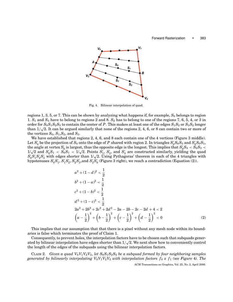
An image-plane quad V0V1V2V3 (see Figure 4) is forward rasterized by bilinear interpolation withinterpolation factors f0 x f1 given by Equation (1).
f0 =⌈√
2 max(V0V1, V2V3)⌉
f1 =⌈√
2 max(V0V3, V1V2)⌉
(1)
We now prove that rasterizing an image-plane mesh of quads using the interpolation factors givenguarantees that every pixel covered by the mesh will receive at least one sample. The proof has twoparts. First, we show that if the quads in a mesh have edges shorter than 1/
√2 pixels, every pixel
covered by the mesh contains a mesh node (i.e. a quad vertex). We call such a mesh a rasterizationmesh. Then we show that Equation (1) generates a rasterization mesh.
CLAIM 1. Every pixel covered by a rasterization mesh contains at least one mesh node.
PROOF. Let’s assume that there is a pixel P covered by a rasterization mesh that does not containa quad vertex. Let S0S1S2S3 be the quad that contains the center of P . Such a quad exists since P ,including its center, is covered by the mesh. Vertices S0, S1,S2, and S3 are outside pixel P since P doesnot contain any vertex. Their possible locations are shown in Figure 3, left. No vertex can belong to
ACM Transactions on Graphics, Vol. 25, No. 2, April 2006.
Forward Rasterization • 383
Fig. 4. Bilinear interpolation of quad.
regions 1, 3, 5, or 7. This can be shown by analyzing what happens if, for example, S0 belongs to region1. S1 and S3 have to belong to regions 2 and 8. S2 has to belong to one of the regions 7, 6, 5, 4, or 3 inorder for S0S1S2S3 to contain the center of P . This makes at least one of the edges S1S2 or S3S2 longerthan 1/
√2. It can be argued similarly that none of the regions 2, 4, 6, or 8 can contain two or more of
the vertices S0, S1,S2, and S3.We have established that regions 2, 4, 6, and 8 each contain one of the 4 vertices (Figure 3 middle).
Let S′0 be the projection of S0 onto the edge of P shared with region 2. In triangles S′
0S0S3 and S′0S0S1,
the angle at vertex S′0 is largest, thus the opposite edge is the longest. This implies that S′
0S3 < S0S3 <
1/√
2 and S′0S1 < S0S1 < 1/
√2. Points S′
1, S′2, and S′
3 are constructed similarly, yielding the quadS′
0S′1S′
2S′3 with edges shorter than 1/
√2. Using Pythagoras’ theorem in each of the 4 triangles with
hypotenuses S′0S′
1, S′1S′
2, S′2S′
3,and S′3S′
0 (Figure 3 right), we reach a contradiction (Equation (2)).
a2 + (1 − d )2 <1
2
b2 + (1 − a)2 <1
2
c2 + (1 − b)2 <1
2
d2 + (1 − c)2 <1
2
2a2 + 2b2 + 2c2 + 2d2 − 2a − 2b − 2c − 2d + 4 < 2(a − 1
2
)2
+(
b − 1
2
)2
+(
c − 1
2
)2
+(
d − 1
2
)2
< 0 (2)
This implies that our assumption that that there is a pixel without any mesh node within its bound-aries is false which terminates the proof of Claim 1.
Consequently, to prevent holes, the interpolation factors have to be chosen such that subquads gener-ated by bilinear interpolation have edges shorter than 1/
√2. We next show how to conveniently control
the length of the edges of the subquads using the bilinear interpolation factors.
CLAIM 2. Given a quad V0V1V2V3, let S0S1S2S3 be a subquad formed by four neighboring samplesgenerated by bilinearly interpolating V0V1V2V3 with interpolation factors f0 x f1 (see Figure 4). The
ACM Transactions on Graphics, Vol. 25, No. 2, April 2006.
384 • V. Popescu and P. Rosen
following inequality holds:
max(S0S1, S2S3) ≤ 1
f0
max(V0V1, V2V3)
max(S1S2, S3S0) ≤ 1
f1
max(V1V2, V3V0). (3)
PROOF. All the segments on a bilinear interpolation row or column have the same length. The samesamples are generated no matter whether the interpolation proceeds in row-major order or in column-major order. Consequently, all we have to do is to show that AB ≤ max(V0V1, V2V3), where A and B arecorresponding points generated on V0V3 and V1V2 (see Figure 4). We derive the proof of the inequalityusing only the x components of AB, V0V1, and V2V3; the y expressions are similar because of symmetry.
V0V 21x
= (xV0
− xV1
)2, V3V 2
2x= (
xV3− xV2
)2, AB2
x = (xA − xB)2
xA = xV0+ (
xV3− xV0
)k
xB = xV1+ (
xV2− xV1
)k
0 ≤ k ≤ 1.
Let
x01 = xV0− xV1
x32 = xV3− xV2
V0V 21x = x2
01
V3V 22x = x2
32,
then
AB2x = (x01 + (x32 − x01)k)2 =
= x201 + (
x232 − x2
01
)k − (
x232 − x2
01
)k + (x32 − x01)2k2 + 2x01(x32 − x01)k =
= V0V 21x + (
V3V 22x − V0V 2
1x
)k − k(x32 − x01)(x32 + x01 − k(x32 − x01) − 2x01) =
= V0V 21x + (
V3V 22x − V0V 2
1x
)k − k(1 − k)(x32 − x01)2 =
= V0V 21x + (
V3V 22x − V0V 2
1x
)k − �x , �x ≥ 0.
Consequently,AB2 ≤ V0V 2
1 + (V3V 22 − V0V 2
1 )k ≤ max(V0V 21 , V3V 2
2 ),which terminates the proof.
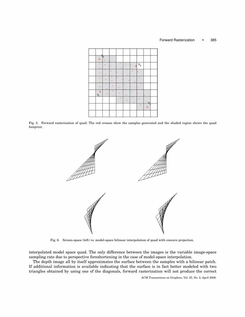
Figure 5 shows the samples generated by forward rasterization with red diagonal crosses. The samplesare independent of the pixel grid. The shaded region shows the quad footprint. All pixels have at leastone sample.
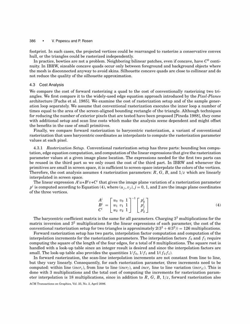
4.2 Bow Ties
The four depth image samples defining the quadrilateral primitive are not necessarily coplanar. Theprojection of the quad could be concave. Forward rasterization, which bilinearly interpolates in screenspace, generates a primitive footprint equivalent to that obtained by model-space bilinear interpolation.In Figure 6, the left wire frames are obtained by forward rasterizing the projection of the quad with 9 ×9 interpolation factors. (The coarse interpolation factors were chosen to show the samples generatedat the intersection of the sampling lines.) The right-hand images were obtained by projecting the 9 × 9
ACM Transactions on Graphics, Vol. 25, No. 2, April 2006.
Forward Rasterization • 385
Fig. 5. Forward rasterization of quad. The red crosses show the samples generated and the shaded region shows the quad
footprint.
Fig. 6. Screen-space (left) vs. model-space bilinear interpolation of quad with concave projection.
interpolated model space quad. The only difference between the images is the variable image-spacesampling rate due to perspective foreshortening in the case of model-space interpolation.
The depth image all by itself approximates the surface between the samples with a bilinear patch.If additional information is available indicating that the surface is in fact better modeled with twotriangles obtained by using one of the diagonals, forward rasterization will not produce the correct
ACM Transactions on Graphics, Vol. 25, No. 2, April 2006.
386 • V. Popescu and P. Rosen
footprint. In such cases, the projected vertices could be rearranged to rasterize a conservative convexhull, or the triangles could be rasterized independently.
In practice, bowties are not a problem. Neighboring bilinear patches, even if concave, have C0 conti-nuity. In IBRW, sizeable concave quads occur only between foreground and background objects wherethe mesh is disconnected anyway to avoid skins. Silhouette concave quads are close to collinear and donot reduce the quality of the silhouette approximation.
4.3 Cost Analysis
We compare the cost of forward rasterizing a quad to the cost of conventionally rasterizing two tri-angles. We first compare it to the widely-used edge equation approach introduced by the Pixel-Planesarchitecture [Fuchs et al. 1985]. We examine the cost of rasterization setup and of the sample gener-ation loop separately. We assume that conventional rasterization executes the inner loop a number oftimes equal to the area of the screen-aligned bounding rectangle of the triangle. Although techniquesfor reducing the number of exterior pixels that are tested have been proposed [Pineda 1988], they comewith additional setup and scan line costs which make the analysis scene dependent and might offsetthe benefits in the case of small primitives.
Finally, we compare forward rasterization to barycentric rasterization, a variant of conventionalrasterization that uses barycentric coordinates as interpolants to compute the rasterization parametervalues at each pixel.
4.3.1 Rasterization Setup. Conventional rasterization setup has three parts: bounding box compu-tation, edge equation computation, and computation of the linear expressions that give the rasterizationparameter values at a given image plane location. The expressions needed for the first two parts canbe reused in the third part so we only count the cost of the third part. In IBRW and whenever theprimitives are small in screen space, it is sufficient to screen-space interpolate the colors of the vertices.Therefore, the cost analysis assumes 4 rasterization parameters: R, G, B, and 1/z which are linearlyinterpolated in screen space.
The linear expression Aiu+Biv+Ci that gives the image plane variation of a rasterization parameterpi is computed according to Equation (4), where (u j , vj ), j = 0, 1, and 2 are the image plane coordinatesof the three vertices.
Ai
Bi
Ci=
⎡⎣ u0 v0 1u1 v1 1u2 v2 1
⎤⎦−1 ⎡⎣ pi0
pi1
pi2
⎤⎦ (4)
The barycentric coefficient matrix is the same for all parameters. Charging 33 multiplications for thematrix inversion and 32 multiplications for the linear expressions of each parameter, the cost of theconventional rasterization setup for two triangles is approximately 2(33 + 4(32)) = 126 multiplications.
Forward rasterization setup has two parts, interpolation factor computation and computation of theinterpolation increments for the rasterization parameters. The interpolation factors f0 and f1 requirecomputing the square of the length of the four edges, for a total of 8 multiplications. The square root ishandled with a look-up table since an integer result is desired and since the interpolation factors aresmall. The look-up table also provides the quantities 1/ f0, 1/ f1 and 1/( f0 f1).
In forward rasterization, the scan-line interpolation increments are not constant from line to line,but they vary linearly. Consequently, for each rasterization parameter, three increments need to becomputed: within line (incrc), from line to line (incrl ), and incrc line to line variation (incrcl ). This isdone with 3 multiplications and the total cost of computing the increments for rasterization param-eter interpolation is 18 multiplications, since in addition to R, G, B, 1/z, forward rasterization also
ACM Transactions on Graphics, Vol. 25, No. 2, April 2006.
Forward Rasterization • 387
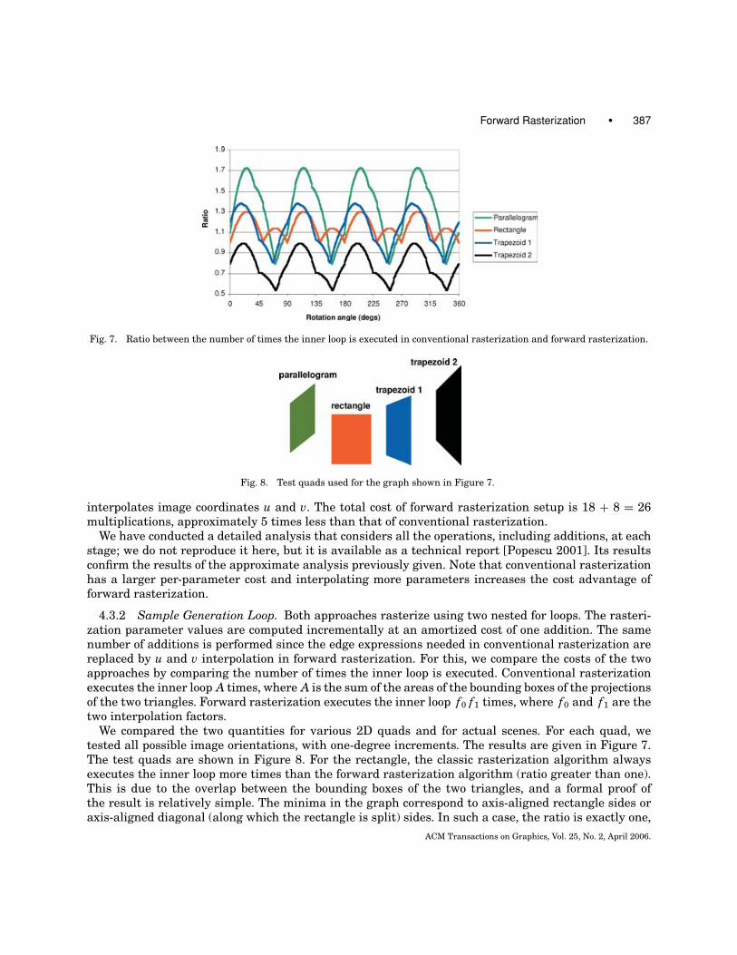
Fig. 7. Ratio between the number of times the inner loop is executed in conventional rasterization and forward rasterization.
Fig. 8. Test quads used for the graph shown in Figure 7.
interpolates image coordinates u and v. The total cost of forward rasterization setup is 18 + 8 = 26multiplications, approximately 5 times less than that of conventional rasterization.
We have conducted a detailed analysis that considers all the operations, including additions, at eachstage; we do not reproduce it here, but it is available as a technical report [Popescu 2001]. Its resultsconfirm the results of the approximate analysis previously given. Note that conventional rasterizationhas a larger per-parameter cost and interpolating more parameters increases the cost advantage offorward rasterization.
4.3.2 Sample Generation Loop. Both approaches rasterize using two nested for loops. The rasteri-zation parameter values are computed incrementally at an amortized cost of one addition. The samenumber of additions is performed since the edge expressions needed in conventional rasterization arereplaced by u and v interpolation in forward rasterization. For this, we compare the costs of the twoapproaches by comparing the number of times the inner loop is executed. Conventional rasterizationexecutes the inner loop A times, where A is the sum of the areas of the bounding boxes of the projectionsof the two triangles. Forward rasterization executes the inner loop f0 f1 times, where f0 and f1 are thetwo interpolation factors.
We compared the two quantities for various 2D quads and for actual scenes. For each quad, wetested all possible image orientations, with one-degree increments. The results are given in Figure 7.The test quads are shown in Figure 8. For the rectangle, the classic rasterization algorithm alwaysexecutes the inner loop more times than the forward rasterization algorithm (ratio greater than one).This is due to the overlap between the bounding boxes of the two triangles, and a formal proof ofthe result is relatively simple. The minima in the graph correspond to axis-aligned rectangle sides oraxis-aligned diagonal (along which the rectangle is split) sides. In such a case, the ratio is exactly one,
ACM Transactions on Graphics, Vol. 25, No. 2, April 2006.
388 • V. Popescu and P. Rosen
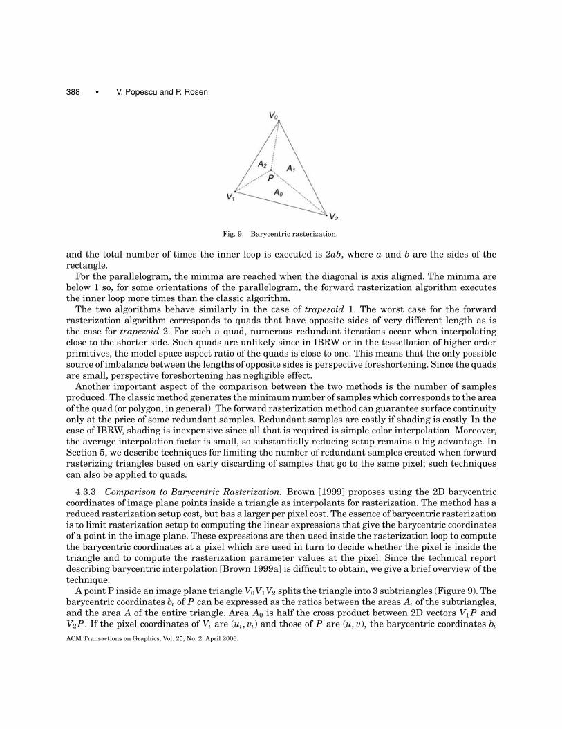
Fig. 9. Barycentric rasterization.
and the total number of times the inner loop is executed is 2ab, where a and b are the sides of therectangle.
For the parallelogram, the minima are reached when the diagonal is axis aligned. The minima arebelow 1 so, for some orientations of the parallelogram, the forward rasterization algorithm executesthe inner loop more times than the classic algorithm.
The two algorithms behave similarly in the case of trapezoid 1. The worst case for the forwardrasterization algorithm corresponds to quads that have opposite sides of very different length as isthe case for trapezoid 2. For such a quad, numerous redundant iterations occur when interpolatingclose to the shorter side. Such quads are unlikely since in IBRW or in the tessellation of higher orderprimitives, the model space aspect ratio of the quads is close to one. This means that the only possiblesource of imbalance between the lengths of opposite sides is perspective foreshortening. Since the quadsare small, perspective foreshortening has negligible effect.
Another important aspect of the comparison between the two methods is the number of samplesproduced. The classic method generates the minimum number of samples which corresponds to the areaof the quad (or polygon, in general). The forward rasterization method can guarantee surface continuityonly at the price of some redundant samples. Redundant samples are costly if shading is costly. In thecase of IBRW, shading is inexpensive since all that is required is simple color interpolation. Moreover,the average interpolation factor is small, so substantially reducing setup remains a big advantage. InSection 5, we describe techniques for limiting the number of redundant samples created when forwardrasterizing triangles based on early discarding of samples that go to the same pixel; such techniquescan also be applied to quads.
4.3.3 Comparison to Barycentric Rasterization. Brown [1999] proposes using the 2D barycentriccoordinates of image plane points inside a triangle as interpolants for rasterization. The method has areduced rasterization setup cost, but has a larger per pixel cost. The essence of barycentric rasterizationis to limit rasterization setup to computing the linear expressions that give the barycentric coordinatesof a point in the image plane. These expressions are then used inside the rasterization loop to computethe barycentric coordinates at a pixel which are used in turn to decide whether the pixel is inside thetriangle and to compute the rasterization parameter values at the pixel. Since the technical reportdescribing barycentric interpolation [Brown 1999a] is difficult to obtain, we give a brief overview of thetechnique.
A point P inside an image plane triangle V0V1V2 splits the triangle into 3 subtriangles (Figure 9). Thebarycentric coordinates bi of P can be expressed as the ratios between the areas Ai of the subtriangles,and the area A of the entire triangle. Area A0 is half the cross product between 2D vectors V1 P andV2 P . If the pixel coordinates of Vi are (ui, vi) and those of P are (u, v), the barycentric coordinates bi
ACM Transactions on Graphics, Vol. 25, No. 2, April 2006.
Forward Rasterization • 389
are given by Equation (5), where the incremented subindices i + 1 and i + 2 are computed modulo 3.
bi = Ai/A
2Ai =∣∣∣∣ ui+1 − u vi+1 − v
ui+2 − u vi+2 − v
∣∣∣∣ = (ui+1 − u) (vi+2 − v) − (ui+2 − u) (vi+1 − v) == (vi+1 − vi+2) u + (ui+2 − ui+1) v + (ui+1vi+2 − ui+2vi+1)
2A =∣∣∣∣ u1 − u0 v1 − v0
u2 − u0 v2 − v0
∣∣∣∣ = (u1 − u0) (v2 − v0) − (u2 − u0) (v1 − v0)
bi = (vi+1 − vi+2)
Au + (ui+2 − ui+1)
Av + (ui+1vi+2 − ui+2vi+1)
Abi = K 0
i u + K 1i v + K 2
i (5)
Each of the 3 barycentric coordinates bi is given by a linear expression with coefficients K0i , K1
i , andK2
i . Ignoring the additions, computing each linear expression takes 2 multiplications and 3 divisions,or 5 multiplications since the denominator is the same. The area of the entire triangle is computedwith two multiplications. The total rasterization setup cost for the triangle is 5 ∗ 3 + 2 = 17 mul-tiplications, or 34 multiplications for 2 triangles. This setup cost is comparable to that of forwardrasterization (26 multiplications). However, barycentric rasterization has a much higher per-samplecost.
In the sample generation loop, for each pixel considered for the given triangle, the first step is tocompute the barycentric coordinates using the linear expressions established at setup. This is done withan amortized cost of 3 additions. If any of the barycentric coordinates is negative, the pixel is outsidethe triangle. When a pixel is inside a triangle, the rasterization parameters have to be computed asan average of the values at the vertices, weighted with the barycentric coordinates. (See Equation (6),where bi(u, v) and r(u, v) are the barycentric coordinates, and the rasterization parameter r at pixel (u,v)). This implies 3 multiplications per rasterization parameter, or 12 multiplications when r, g , b, andz are desired.
r(u, v) = r(u0, v0)b0(u, v) + r(u1, v1)b1(u, v) + r(u2, v2)b2(u, v) (6)
In conclusion, in the case of IBRW, barycentric rasterization has a setup cost comparable to that offorward rasterization but deviates significantly from the optimal cost of 1 addition per pixel, per raster-ization parameter. This implies that barycentric interpolation is comparable to forward rasterizationonly for quads that are so small as to not cover any pixels. A quad that covers 5 pixels requires 60additional multiplications in the case of barycentric rasterization.
5. FORWARD RASTERIZATION OF TRIANGLES
5.1 Interpolation
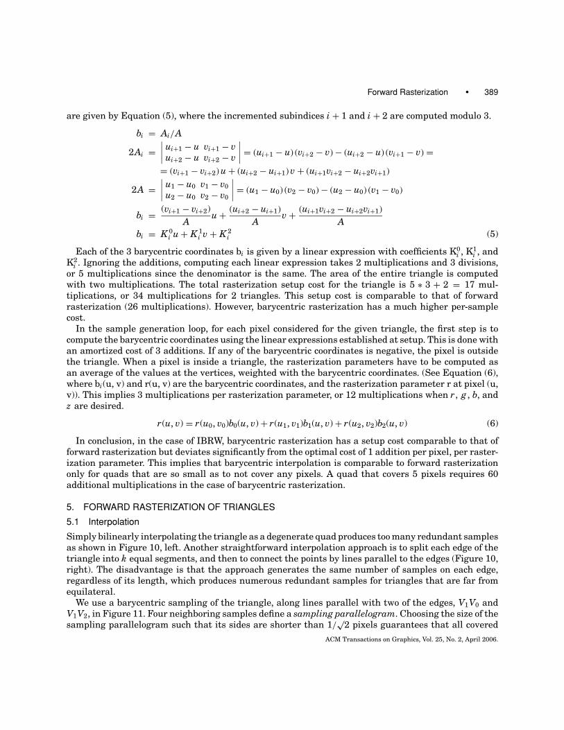
Simply bilinearly interpolating the triangle as a degenerate quad produces too many redundant samplesas shown in Figure 10, left. Another straightforward interpolation approach is to split each edge of thetriangle into k equal segments, and then to connect the points by lines parallel to the edges (Figure 10,right). The disadvantage is that the approach generates the same number of samples on each edge,regardless of its length, which produces numerous redundant samples for triangles that are far fromequilateral.
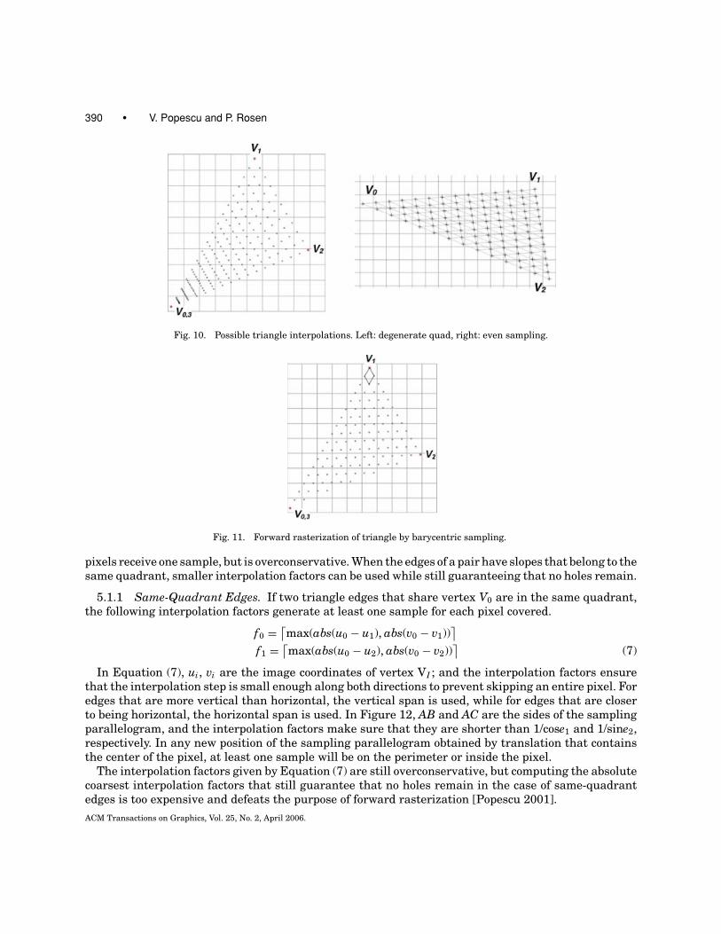
We use a barycentric sampling of the triangle, along lines parallel with two of the edges, V1V0 andV1V2, in Figure 11. Four neighboring samples define a sampling parallelogram. Choosing the size of thesampling parallelogram such that its sides are shorter than 1/
√2 pixels guarantees that all covered
ACM Transactions on Graphics, Vol. 25, No. 2, April 2006.
390 • V. Popescu and P. Rosen
Fig. 10. Possible triangle interpolations. Left: degenerate quad, right: even sampling.
Fig. 11. Forward rasterization of triangle by barycentric sampling.
pixels receive one sample, but is overconservative. When the edges of a pair have slopes that belong to thesame quadrant, smaller interpolation factors can be used while still guaranteeing that no holes remain.
5.1.1 Same-Quadrant Edges. If two triangle edges that share vertex V0 are in the same quadrant,the following interpolation factors generate at least one sample for each pixel covered.
f0 = ⌈max(abs(u0 − u1), abs(v0 − v1))
⌉f1 = ⌈
max(abs(u0 − u2), abs(v0 − v2))⌉
(7)
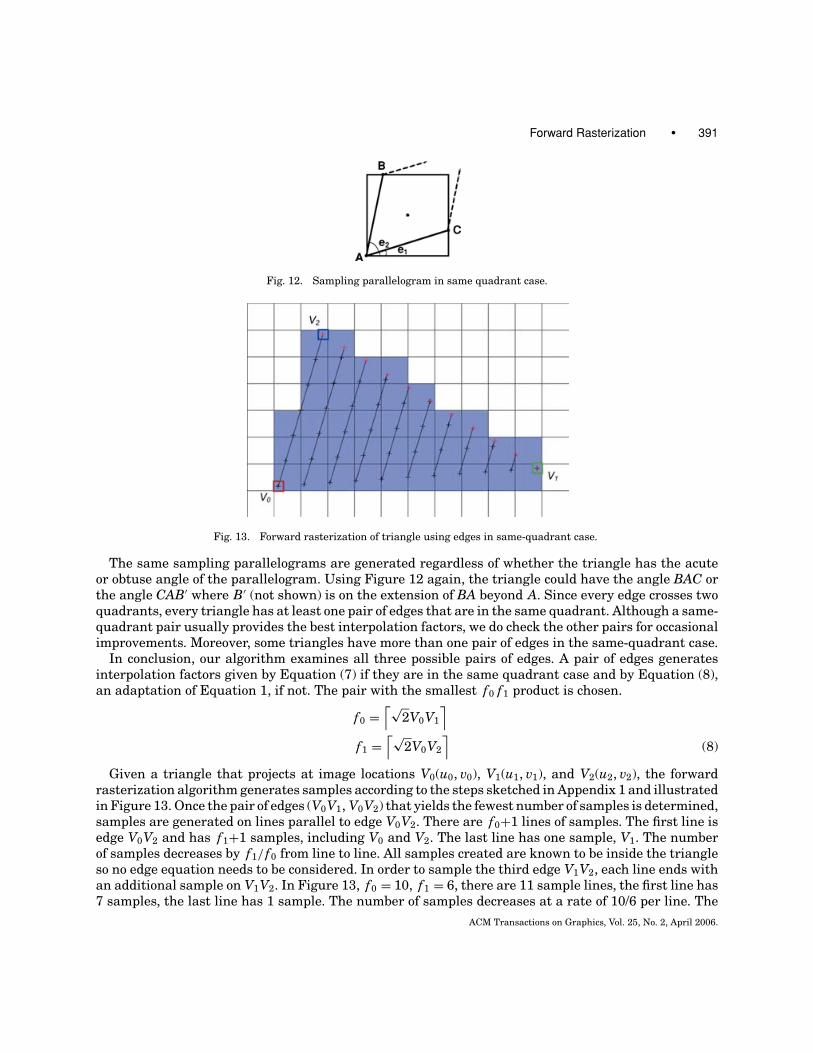
In Equation (7), ui, vi are the image coordinates of vertex VI ; and the interpolation factors ensurethat the interpolation step is small enough along both directions to prevent skipping an entire pixel. Foredges that are more vertical than horizontal, the vertical span is used, while for edges that are closerto being horizontal, the horizontal span is used. In Figure 12, AB and AC are the sides of the samplingparallelogram, and the interpolation factors make sure that they are shorter than 1/cose1 and 1/sine2,respectively. In any new position of the sampling parallelogram obtained by translation that containsthe center of the pixel, at least one sample will be on the perimeter or inside the pixel.
The interpolation factors given by Equation (7) are still overconservative, but computing the absolutecoarsest interpolation factors that still guarantee that no holes remain in the case of same-quadrantedges is too expensive and defeats the purpose of forward rasterization [Popescu 2001].
ACM Transactions on Graphics, Vol. 25, No. 2, April 2006.
Forward Rasterization • 391
Fig. 12. Sampling parallelogram in same quadrant case.
Fig. 13. Forward rasterization of triangle using edges in same-quadrant case.
The same sampling parallelograms are generated regardless of whether the triangle has the acuteor obtuse angle of the parallelogram. Using Figure 12 again, the triangle could have the angle BAC orthe angle CAB′ where B′ (not shown) is on the extension of BA beyond A. Since every edge crosses twoquadrants, every triangle has at least one pair of edges that are in the same quadrant. Although a same-quadrant pair usually provides the best interpolation factors, we do check the other pairs for occasionalimprovements. Moreover, some triangles have more than one pair of edges in the same-quadrant case.
In conclusion, our algorithm examines all three possible pairs of edges. A pair of edges generatesinterpolation factors given by Equation (7) if they are in the same quadrant case and by Equation (8),an adaptation of Equation 1, if not. The pair with the smallest f0 f1 product is chosen.
f0 =⌈√
2V0V1
⌉f1 =
⌈√2V0V2
⌉(8)
Given a triangle that projects at image locations V0(u0, v0), V1(u1, v1), and V2(u2, v2), the forwardrasterization algorithm generates samples according to the steps sketched in Appendix 1 and illustratedin Figure 13. Once the pair of edges (V0V1, V0V2) that yields the fewest number of samples is determined,samples are generated on lines parallel to edge V0V2. There are f0+1 lines of samples. The first line isedge V0V2 and has f1+1 samples, including V0 and V2. The last line has one sample, V1. The numberof samples decreases by f1/ f0 from line to line. All samples created are known to be inside the triangleso no edge equation needs to be considered. In order to sample the third edge V1V2, each line ends withan additional sample on V1V2. In Figure 13, f0 = 10, f1 = 6, there are 11 sample lines, the first line has7 samples, the last line has 1 sample. The number of samples decreases at a rate of 10/6 per line. The
ACM Transactions on Graphics, Vol. 25, No. 2, April 2006.
392 • V. Popescu and P. Rosen
samples generated on V1V2 are shown in red. The pixels that receive at least a sample are highlightedin grey.
5.2 Cost Analysis
As in the case of IBRW, we first compare the cost of forward rasterization to the cost of edge equationrasterization and then to the cost of barycentric rasterization.
5.2.1 Rasterization Setup. We have seen that the conventional rasterization setup cost for a trianglein the case of the edge equation approach is approximately 63 multiplications. The forward rasterizationalgorithm described first finds the interpolation factors using Equation (7) and Equation (8). The squareof the lengths of the three edges cost 6 multiplications; deciding whether each pair of edges is in thesame quadrant case has a total cost of another 6 multiplications. The square root needed by Equation (8)is looked up in a table, along with the values 1/ f0 1/ f1, and 1/( f0 f1). Then the rasterization parameterincrements are computed along each of the three edges, at a total cost of 18 multiplications, assumingthat R, G, B, u, v, and z are interpolated. The total forward rasterization setup cost for a triangle is 30multiplications, approximately half of that of conventional rasterization.
5.2.2 Sample Generation Loop. The amortized per-sample cost is one addition per-rasterizationparameter for both conventional and forward rasterization algorithms. We compare the performanceof the sample generation loop by analyzing the number of times the inner loop is evaluated ILN, thenumber of samples generated SGN, and the number of pixels set PSN. The triangle in Figure 13 hasa 10 by 6 pixel bounding box and thus, for the conventional rasterization, ILN = 60. For the forwardrasterization algorithm ILN = 50, including the samples on the third edge. PSN is 29 and 39 forconventional and forward rasterization, respectively. Conventional rasterization generates a sampleonly if it is inside the triangle, thus SGN = PSN = 29. The algorithm described generates ILN = 50samples which means that ILN – PSN = 11 pixels are overwritten. Redundant samples are particularlycostly when shading is expensive, for example, involving several texture look ups. It is possible thatsamples within a pixel are sorted in back-to-front order, in which case deferring shading until aftervisibility does not help.
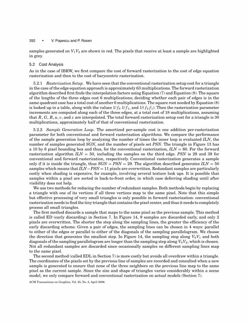
We use two methods for reducing the number of redundant samples. Both methods begin by replacinga triangle with one of its vertices if all three vertices map to the same pixel. Note that this simplebut effective processing of very small triangles is only possible in forward rasterization: conventionalrasterization needs to find the tiny triangle that contains the pixel center, and thus it needs to completelyprocess all small triangles.
The first method discards a sample that maps to the same pixel as the previous sample. This methodis called ED (early discarding) in Section 7. In Figure 14, 9 samples are discarded early, and only 2pixels are overwritten. The shorter the step along the sampling lines, the greater the efficiency of theearly discarding scheme. Given a pair of edges, the sampling lines can be chosen in 4 ways: parallelto either of the edges or parallel to either of the diagonals of the sampling parallelogram. We choosethe direction that generates the smallest step. In Figure 14, the sampling step along V0V1 and bothdiagonals of the sampling parallelogram are longer than the sampling step along V0V2, which is chosen.Not all redundant samples are discarded since occasionally samples on different sampling lines mapto the same pixel.
The second method (called EDL in Section 7) is more costly but avoids all overdraw within a triangle.The coordinates of the pixels set by the previous line of samples are recorded and consulted when a newsample is generated to ensure that none of the three neighbors on the previous line map to the samepixel as the current sample. Since the size and shape of triangles varies considerably within a scenemodel, we only compare forward and conventional rasterization on actual models (Section 7).
ACM Transactions on Graphics, Vol. 25, No. 2, April 2006.

Forward Rasterization • 393
Fig. 14. Early discarded samples shown with black squares.
Fig. 15. Z-buffering along different rays in forward rasterization.
5.2.3 Comparison to Barycentric Rasterization. As shown earlier, the cost of barycentric rasteriza-tion setup is 17 multiplications which is lower than the 30 multiplications required by forward rasteri-zation. However, this comes at the price of 3 multiplications per-rasterization parameter and per pixel,whereas forward rasterization, or edge equation rasterization for that matter, does not require any. Inpolygonal rendering, the number of rasterization parameters that are used as ingredients for the finalpixel color is far larger than the 4 used in IBRW. Two-dimensional texture coordinates and 3D normalsbring the tally to 9 rasterization parameters which require 27 multiplications per pixel. Except for verysmall (subpixel) triangles, the cost of barycentric interpolation makes it unattractive.
6. OFFSET RECONSTRUCTION
In forward rasterization, no inverse mapping from the image plane to the primitive is computed, thusone cannot generate a sample at a particular image plane location. The pixel grid is ignored exceptfor determining interpolation factors that are sufficient to cover all pixels. The samples generated byforward rasterization can land anywhere inside the pixel. This has implications in z-buffering and inreconstruction/resampling.
6.1 Z-Buffering
Z-buffering samples that land at different locations within the pixel reduces the precision of the z test,since the samples belong to different desired image rays. In Figure 15, the samples P0 and P1 are
ACM Transactions on Graphics, Vol. 25, No. 2, April 2006.
394 • V. Popescu and P. Rosen
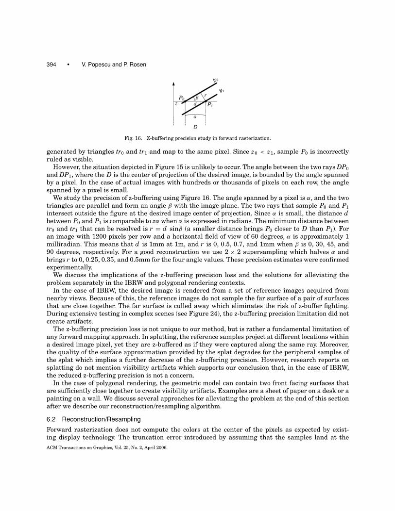
Fig. 16. Z-buffering precision study in forward rasterization.
generated by triangles tr0 and tr1 and map to the same pixel. Since z0 < z1, sample P0 is incorrectlyruled as visible.
However, the situation depicted in Figure 15 is unlikely to occur. The angle between the two rays DP0
and DP1, where the D is the center of projection of the desired image, is bounded by the angle spannedby a pixel. In the case of actual images with hundreds or thousands of pixels on each row, the anglespanned by a pixel is small.
We study the precision of z-buffering using Figure 16. The angle spanned by a pixel is α, and the twotriangles are parallel and form an angle β with the image plane. The two rays that sample P0 and P1
intersect outside the figure at the desired image center of projection. Since α is small, the distance dbetween P0 and P1 is comparable to zα when α is expressed in radians. The minimum distance betweentr0 and tr1 that can be resolved is r = d sinβ (a smaller distance brings P0 closer to D than P1). Foran image with 1200 pixels per row and a horizontal field of view of 60 degrees, α is approximately 1milliradian. This means that d is 1mm at 1m, and r is 0, 0.5, 0.7, and 1mm when β is 0, 30, 45, and90 degrees, respectively. For a good reconstruction we use 2 × 2 supersampling which halves α andbrings r to 0, 0.25, 0.35, and 0.5mm for the four angle values. These precision estimates were confirmedexperimentally.
We discuss the implications of the z-buffering precision loss and the solutions for alleviating theproblem separately in the IBRW and polygonal rendering contexts.
In the case of IBRW, the desired image is rendered from a set of reference images acquired fromnearby views. Because of this, the reference images do not sample the far surface of a pair of surfacesthat are close together. The far surface is culled away which eliminates the risk of z-buffer fighting.During extensive testing in complex scenes (see Figure 24), the z-buffering precision limitation did notcreate artifacts.
The z-buffering precision loss is not unique to our method, but is rather a fundamental limitation ofany forward mapping approach. In splatting, the reference samples project at different locations withina desired image pixel, yet they are z-buffered as if they were captured along the same ray. Moreover,the quality of the surface approximation provided by the splat degrades for the peripheral samples ofthe splat which implies a further decrease of the z-buffering precision. However, research reports onsplatting do not mention visibility artifacts which supports our conclusion that, in the case of IBRW,the reduced z-buffering precision is not a concern.
In the case of polygonal rendering, the geometric model can contain two front facing surfaces thatare sufficiently close together to create visibility artifacts. Examples are a sheet of paper on a desk or apainting on a wall. We discuss several approaches for alleviating the problem at the end of this sectionafter we describe our reconstruction/resampling algorithm.
6.2 Reconstruction/Resampling
Forward rasterization does not compute the colors at the center of the pixels as expected by exist-ing display technology. The truncation error introduced by assuming that the samples land at the
ACM Transactions on Graphics, Vol. 25, No. 2, April 2006.
Forward Rasterization • 395
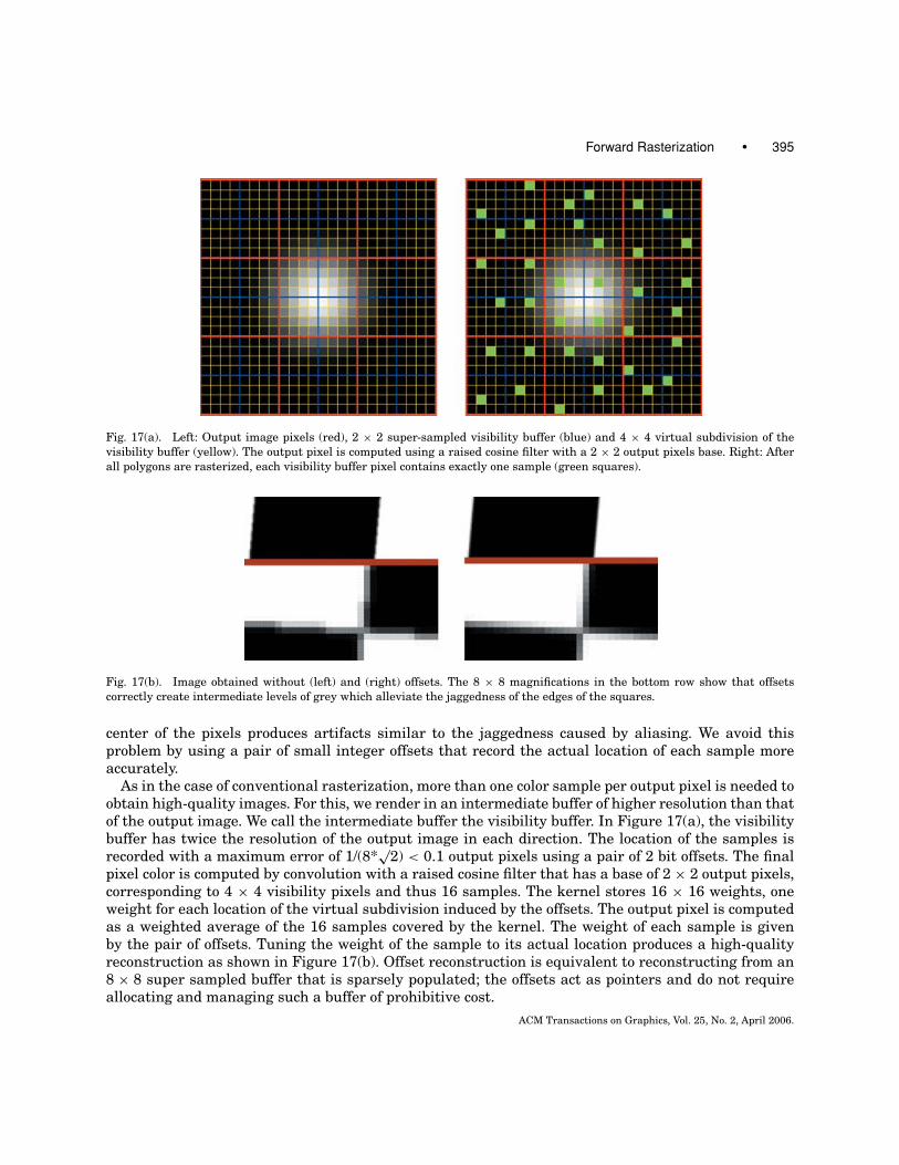
Fig. 17(a). Left: Output image pixels (red), 2 × 2 super-sampled visibility buffer (blue) and 4 × 4 virtual subdivision of the
visibility buffer (yellow). The output pixel is computed using a raised cosine filter with a 2 × 2 output pixels base. Right: After
all polygons are rasterized, each visibility buffer pixel contains exactly one sample (green squares).
Fig. 17(b). Image obtained without (left) and (right) offsets. The 8 × 8 magnifications in the bottom row show that offsets
correctly create intermediate levels of grey which alleviate the jaggedness of the edges of the squares.
center of the pixels produces artifacts similar to the jaggedness caused by aliasing. We avoid thisproblem by using a pair of small integer offsets that record the actual location of each sample moreaccurately.
As in the case of conventional rasterization, more than one color sample per output pixel is needed toobtain high-quality images. For this, we render in an intermediate buffer of higher resolution than thatof the output image. We call the intermediate buffer the visibility buffer. In Figure 17(a), the visibilitybuffer has twice the resolution of the output image in each direction. The location of the samples isrecorded with a maximum error of 1/(8*
√2) < 0.1 output pixels using a pair of 2 bit offsets. The final
pixel color is computed by convolution with a raised cosine filter that has a base of 2 × 2 output pixels,corresponding to 4 × 4 visibility pixels and thus 16 samples. The kernel stores 16 × 16 weights, oneweight for each location of the virtual subdivision induced by the offsets. The output pixel is computedas a weighted average of the 16 samples covered by the kernel. The weight of each sample is givenby the pair of offsets. Tuning the weight of the sample to its actual location produces a high-qualityreconstruction as shown in Figure 17(b). Offset reconstruction is equivalent to reconstructing from an8 × 8 super sampled buffer that is sparsely populated; the offsets act as pointers and do not requireallocating and managing such a buffer of prohibitive cost.
ACM Transactions on Graphics, Vol. 25, No. 2, April 2006.
396 • V. Popescu and P. Rosen
Fig. 18(a). Pixel intensity variation with various reconstruction techniques.
Offset reconstruction implements the inverse mapping from the image plane to the primitive andallows computing the color at the center of the output pixel. When compared to conventional rasteri-zation, one advantage is improved performance. The inverse mapping is computed after visibility, thusonly for the visible samples. The inverse mapping is also considerably less expensive than conventionalrasterization setup: the main additional cost is storing 4 bits at every visibility buffer pixel.
Another advantage is improved quality for both single frames and frame sequences. When super-sampling is used in conventional rasterization, the input samples (reference image color samples forIBRW or triangle vertex colors for triangle meshes), are first blended to create the color samples atthe supersampling locations, and then these color samples are blended again to create the final image.This additional resampling is avoided in the case of forward rasterization where the original referencesamples are filtered only once to produce the final image pixels. This advantage is important for smallprimitives when the density of original samples per output pixel is large. Offset reconstruction producessharper images, an advantage illustrated in Section 7, Figure 25, in the case of an actual model. Offsetreconstruction also has good temporal antialiasing properties.
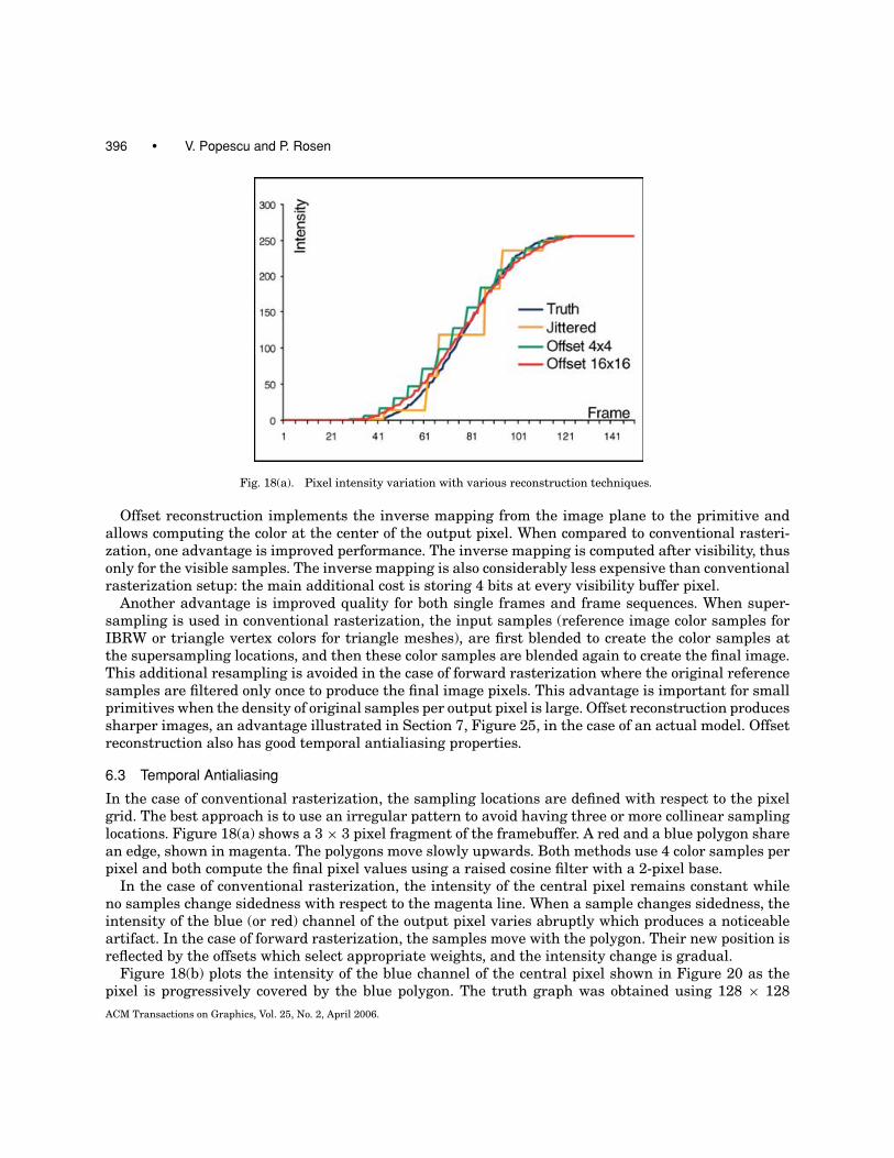
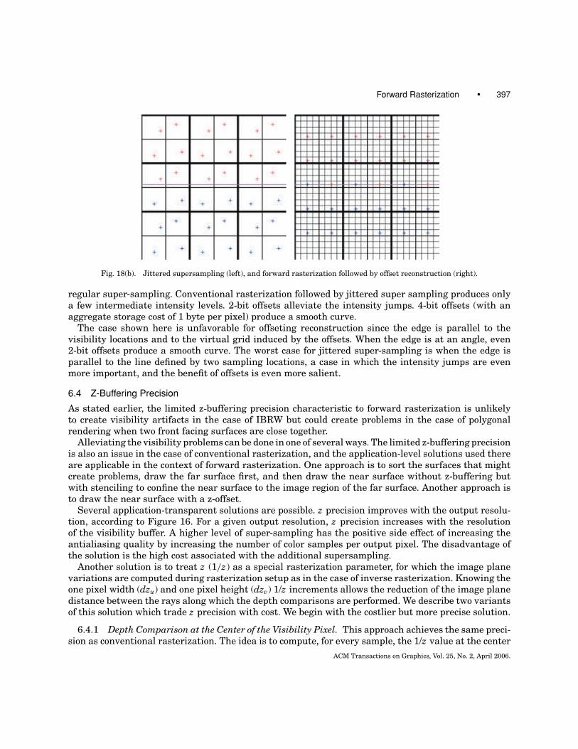
6.3 Temporal Antialiasing
In the case of conventional rasterization, the sampling locations are defined with respect to the pixelgrid. The best approach is to use an irregular pattern to avoid having three or more collinear samplinglocations. Figure 18(a) shows a 3 × 3 pixel fragment of the framebuffer. A red and a blue polygon sharean edge, shown in magenta. The polygons move slowly upwards. Both methods use 4 color samples perpixel and both compute the final pixel values using a raised cosine filter with a 2-pixel base.
In the case of conventional rasterization, the intensity of the central pixel remains constant whileno samples change sidedness with respect to the magenta line. When a sample changes sidedness, theintensity of the blue (or red) channel of the output pixel varies abruptly which produces a noticeableartifact. In the case of forward rasterization, the samples move with the polygon. Their new position isreflected by the offsets which select appropriate weights, and the intensity change is gradual.
Figure 18(b) plots the intensity of the blue channel of the central pixel shown in Figure 20 as thepixel is progressively covered by the blue polygon. The truth graph was obtained using 128 × 128
ACM Transactions on Graphics, Vol. 25, No. 2, April 2006.
Forward Rasterization • 397
Fig. 18(b). Jittered supersampling (left), and forward rasterization followed by offset reconstruction (right).
regular super-sampling. Conventional rasterization followed by jittered super sampling produces onlya few intermediate intensity levels. 2-bit offsets alleviate the intensity jumps. 4-bit offsets (with anaggregate storage cost of 1 byte per pixel) produce a smooth curve.
The case shown here is unfavorable for offseting reconstruction since the edge is parallel to thevisibility locations and to the virtual grid induced by the offsets. When the edge is at an angle, even2-bit offsets produce a smooth curve. The worst case for jittered super-sampling is when the edge isparallel to the line defined by two sampling locations, a case in which the intensity jumps are evenmore important, and the benefit of offsets is even more salient.
6.4 Z-Buffering Precision
As stated earlier, the limited z-buffering precision characteristic to forward rasterization is unlikelyto create visibility artifacts in the case of IBRW but could create problems in the case of polygonalrendering when two front facing surfaces are close together.
Alleviating the visibility problems can be done in one of several ways. The limited z-buffering precisionis also an issue in the case of conventional rasterization, and the application-level solutions used thereare applicable in the context of forward rasterization. One approach is to sort the surfaces that mightcreate problems, draw the far surface first, and then draw the near surface without z-buffering butwith stenciling to confine the near surface to the image region of the far surface. Another approach isto draw the near surface with a z-offset.
Several application-transparent solutions are possible. z precision improves with the output resolu-tion, according to Figure 16. For a given output resolution, z precision increases with the resolutionof the visibility buffer. A higher level of super-sampling has the positive side effect of increasing theantialiasing quality by increasing the number of color samples per output pixel. The disadvantage ofthe solution is the high cost associated with the additional supersampling.
Another solution is to treat z (1/z) as a special rasterization parameter, for which the image planevariations are computed during rasterization setup as in the case of inverse rasterization. Knowing theone pixel width (dzu) and one pixel height (dzv) 1/z increments allows the reduction of the image planedistance between the rays along which the depth comparisons are performed. We describe two variantsof this solution which trade z precision with cost. We begin with the costlier but more precise solution.
6.4.1 Depth Comparison at the Center of the Visibility Pixel. This approach achieves the same preci-sion as conventional rasterization. The idea is to compute, for every sample, the 1/z value at the center
ACM Transactions on Graphics, Vol. 25, No. 2, April 2006.
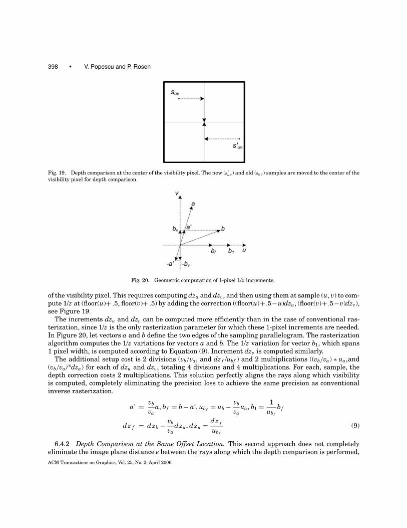
398 • V. Popescu and P. Rosen
Fig. 19. Depth comparison at the center of the visibility pixel. The new (s′uv) and old (suv) samples are moved to the center of the
visibility pixel for depth comparison.
Fig. 20. Geometric computation of 1-pixel 1/z increments.
of the visibility pixel. This requires computing dzu and dzv, and then using them at sample (u, v) to com-pute 1/z at (floor(u)+ .5, floor(v)+ .5) by adding the correction ((floor(u)+ .5−u)dzu, (floor(v)+ .5−v)dzv),see Figure 19.
The increments dzu and dzv can be computed more efficiently than in the case of conventional ras-terization, since 1/z is the only rasterization parameter for which these 1-pixel increments are needed.In Figure 20, let vectors a and b define the two edges of the sampling parallelogram. The rasterizationalgorithm computes the 1/z variations for vectors a and b. The 1/z variation for vector b1, which spans1 pixel width, is computed according to Equation (9). Increment dzv is computed similarly.
The additional setup cost is 2 divisions (vb/va, and dz f /ubf ) and 2 multiplications ((vb/va) ∗ ua,and(vb/va)*dza) for each of dzu and dzv, totaling 4 divisions and 4 multiplications. For each, sample, thedepth correction costs 2 multiplications. This solution perfectly aligns the rays along which visibilityis computed, completely eliminating the precision loss to achieve the same precision as conventionalinverse rasterization.
a′ = vb
vaa, bf = b − a′, ubf = ub − vb
vaua, b1 = 1
ubf
bf
dz f = dzb − vb
vadza, dzu = dz f
ubf
(9)
6.4.2 Depth Comparison at the Same Offset Location. This second approach does not completelyeliminate the image plane distance e between the rays along which the depth comparison is performed,
ACM Transactions on Graphics, Vol. 25, No. 2, April 2006.
Forward Rasterization • 399
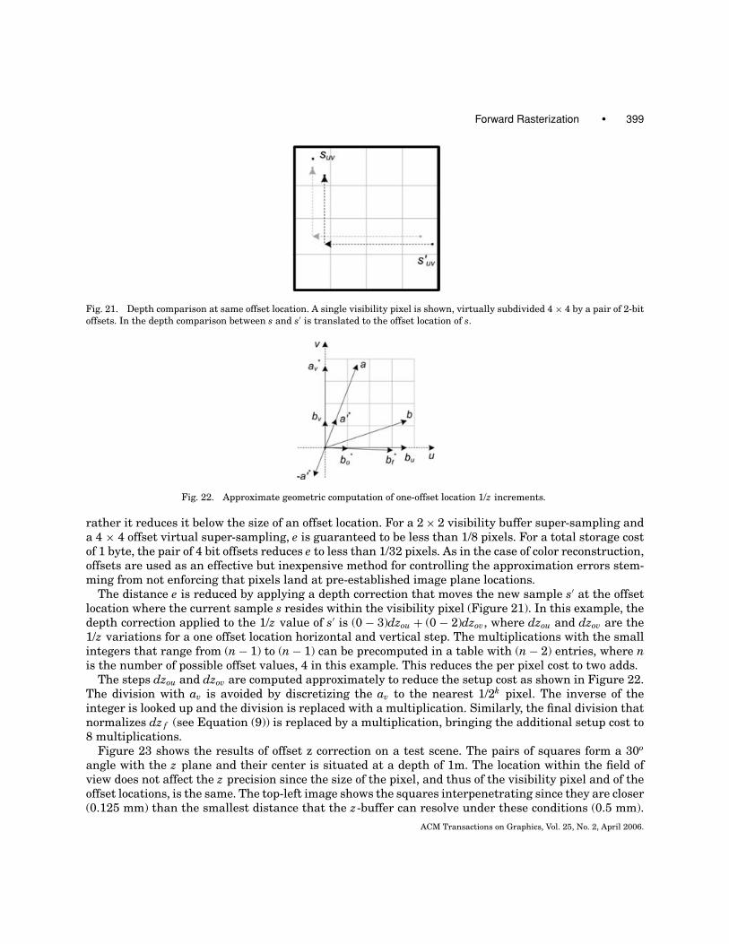
Fig. 21. Depth comparison at same offset location. A single visibility pixel is shown, virtually subdivided 4 × 4 by a pair of 2-bit
offsets. In the depth comparison between s and s′ is translated to the offset location of s.
Fig. 22. Approximate geometric computation of one-offset location 1/z increments.
rather it reduces it below the size of an offset location. For a 2 × 2 visibility buffer super-sampling anda 4 × 4 offset virtual super-sampling, e is guaranteed to be less than 1/8 pixels. For a total storage costof 1 byte, the pair of 4 bit offsets reduces e to less than 1/32 pixels. As in the case of color reconstruction,offsets are used as an effective but inexpensive method for controlling the approximation errors stem-ming from not enforcing that pixels land at pre-established image plane locations.
The distance e is reduced by applying a depth correction that moves the new sample s′ at the offsetlocation where the current sample s resides within the visibility pixel (Figure 21). In this example, thedepth correction applied to the 1/z value of s′ is (0 − 3)dzou + (0 − 2)dzov, where dzou and dzov are the1/z variations for a one offset location horizontal and vertical step. The multiplications with the smallintegers that range from (n − 1) to (n − 1) can be precomputed in a table with (n − 2) entries, where nis the number of possible offset values, 4 in this example. This reduces the per pixel cost to two adds.
The steps dzou and dzov are computed approximately to reduce the setup cost as shown in Figure 22.The division with av is avoided by discretizing the av to the nearest 1/2k pixel. The inverse of theinteger is looked up and the division is replaced with a multiplication. Similarly, the final division thatnormalizes dz f (see Equation (9)) is replaced by a multiplication, bringing the additional setup cost to8 multiplications.
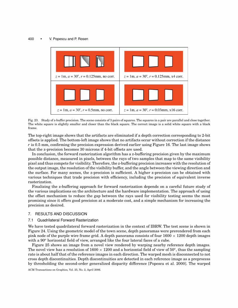
Figure 23 shows the results of offset z correction on a test scene. The pairs of squares form a 30o
angle with the z plane and their center is situated at a depth of 1m. The location within the field ofview does not affect the z precision since the size of the pixel, and thus of the visibility pixel and of theoffset locations, is the same. The top-left image shows the squares interpenetrating since they are closer(0.125 mm) than the smallest distance that the z-buffer can resolve under these conditions (0.5 mm).
ACM Transactions on Graphics, Vol. 25, No. 2, April 2006.
400 • V. Popescu and P. Rosen
Fig. 23. Study of z-buffer precision. The scene consists of 3 pairs of squares. The squares in a pair are parallel and close together.
The white square is slightly smaller and closer than the black square. The correct image is a solid white square with a black
frame.
The top-right image shows that the artifacts are eliminated if a depth correction corresponding to 2-bitoffsets is applied. The bottom-left image shows that no artifacts occur without correction if the distancer is 0.5 mm, confirming the precision expression derived earlier using Figure 16. The last image showsthat the z-precision becomes 30 microns if 4-bit offsets are used.
In conclusion, the forward rasterization algorithm has a z-buffering precision given by the maximumpossible distance, measured in pixels, between the rays of two samples that map to the same visibilitypixel and thus compete for visibility. Therefore, the z-buffering precision increases with the resolution ofthe output image, the resolution of the visibility buffer, and the angle between the viewing direction andthe surface. For many scenes, the z-precision is sufficient. A higher z-precision can be obtained withvarious techniques that trade precision with efficiency, including the precision of equivalent inverserasterization.
Finalizing the z-buffering approach for forward rasterization depends on a careful future study ofthe various implications on the architecture and the hardware implementation. The approach of usingthe offset mechanism to reduce the gap between the rays used for visibility testing seems the mostpromising since it offers good precision at a moderate cost, and a simple mechanism for increasing theprecision as desired.
7. RESULTS AND DISCUSSION
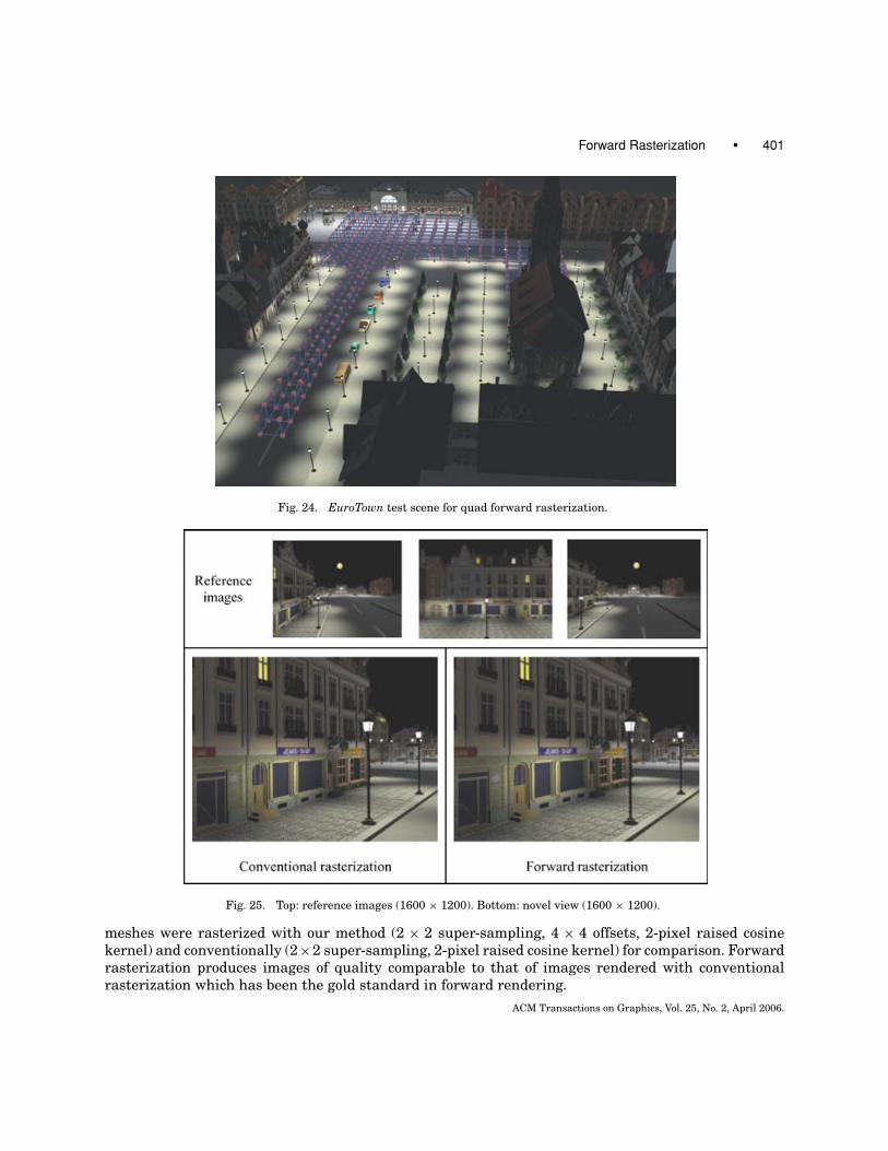
7.1 Quadrilateral Forward Rasterization
We have tested quadrilateral forward rasterization in the context of IBRW. The test scene is shown inFigure 24. Using the geometric model of the town scene, depth panoramas were prerendered from eachpink node of the purple wire frame grid. A depth panorama consists of four 1600 × 1200 depth imageswith a 90o horizontal field of view, arranged like the four lateral faces of a cube.
Figure 25 shows an image from a novel view rendered by warping nearby reference depth images.The novel view has a resolution of 1600 × 1200 and a horizontal field of view of 50o, thus the samplingrate is about half that of the reference images in each direction. The warped mesh is disconnected to notcross depth discontinuities. Depth discontinuities are detected in each reference image as a preprocessby thresholding the second-order generalized disparity difference [Popescu et al. 2000]. The warped
ACM Transactions on Graphics, Vol. 25, No. 2, April 2006.
Forward Rasterization • 401
Fig. 24. EuroTown test scene for quad forward rasterization.
Fig. 25. Top: reference images (1600 × 1200). Bottom: novel view (1600 × 1200).
meshes were rasterized with our method (2 × 2 super-sampling, 4 × 4 offsets, 2-pixel raised cosinekernel) and conventionally (2×2 super-sampling, 2-pixel raised cosine kernel) for comparison. Forwardrasterization produces images of quality comparable to that of images rendered with conventionalrasterization which has been the gold standard in forward rendering.
ACM Transactions on Graphics, Vol. 25, No. 2, April 2006.
402 • V. Popescu and P. Rosen
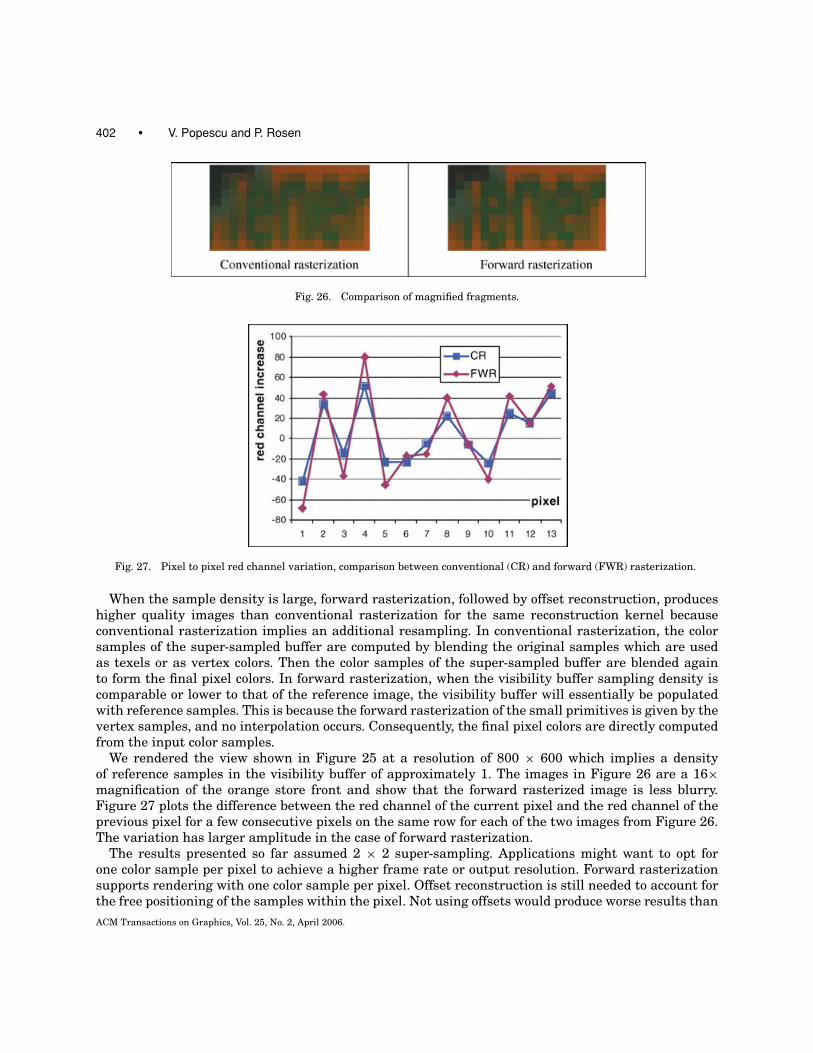
Fig. 26. Comparison of magnified fragments.
Fig. 27. Pixel to pixel red channel variation, comparison between conventional (CR) and forward (FWR) rasterization.
When the sample density is large, forward rasterization, followed by offset reconstruction, produceshigher quality images than conventional rasterization for the same reconstruction kernel becauseconventional rasterization implies an additional resampling. In conventional rasterization, the colorsamples of the super-sampled buffer are computed by blending the original samples which are usedas texels or as vertex colors. Then the color samples of the super-sampled buffer are blended againto form the final pixel colors. In forward rasterization, when the visibility buffer sampling density iscomparable or lower to that of the reference image, the visibility buffer will essentially be populatedwith reference samples. This is because the forward rasterization of the small primitives is given by thevertex samples, and no interpolation occurs. Consequently, the final pixel colors are directly computedfrom the input color samples.
We rendered the view shown in Figure 25 at a resolution of 800 × 600 which implies a densityof reference samples in the visibility buffer of approximately 1. The images in Figure 26 are a 16×magnification of the orange store front and show that the forward rasterized image is less blurry.Figure 27 plots the difference between the red channel of the current pixel and the red channel of theprevious pixel for a few consecutive pixels on the same row for each of the two images from Figure 26.The variation has larger amplitude in the case of forward rasterization.
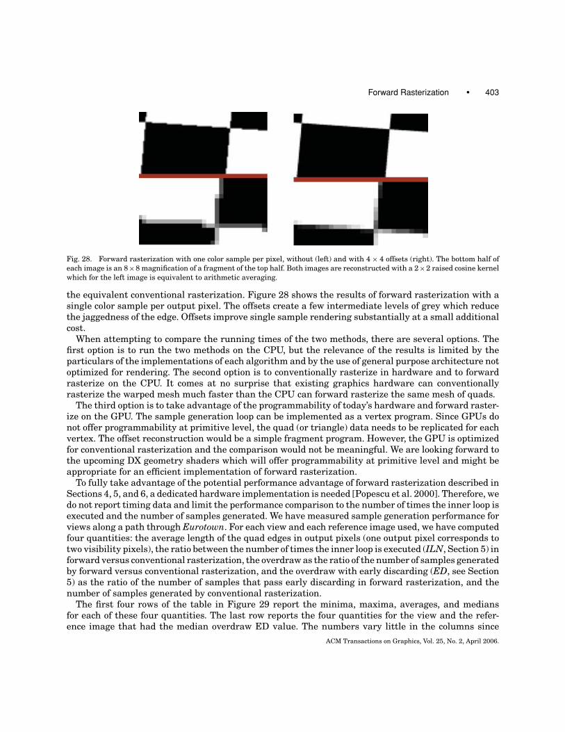
The results presented so far assumed 2 × 2 super-sampling. Applications might want to opt forone color sample per pixel to achieve a higher frame rate or output resolution. Forward rasterizationsupports rendering with one color sample per pixel. Offset reconstruction is still needed to account forthe free positioning of the samples within the pixel. Not using offsets would produce worse results than
ACM Transactions on Graphics, Vol. 25, No. 2, April 2006.
Forward Rasterization • 403
Fig. 28. Forward rasterization with one color sample per pixel, without (left) and with 4 × 4 offsets (right). The bottom half of
each image is an 8×8 magnification of a fragment of the top half. Both images are reconstructed with a 2×2 raised cosine kernel
which for the left image is equivalent to arithmetic averaging.
the equivalent conventional rasterization. Figure 28 shows the results of forward rasterization with asingle color sample per output pixel. The offsets create a few intermediate levels of grey which reducethe jaggedness of the edge. Offsets improve single sample rendering substantially at a small additionalcost.
When attempting to compare the running times of the two methods, there are several options. Thefirst option is to run the two methods on the CPU, but the relevance of the results is limited by theparticulars of the implementations of each algorithm and by the use of general purpose architecture notoptimized for rendering. The second option is to conventionally rasterize in hardware and to forwardrasterize on the CPU. It comes at no surprise that existing graphics hardware can conventionallyrasterize the warped mesh much faster than the CPU can forward rasterize the same mesh of quads.
The third option is to take advantage of the programmability of today’s hardware and forward raster-ize on the GPU. The sample generation loop can be implemented as a vertex program. Since GPUs donot offer programmability at primitive level, the quad (or triangle) data needs to be replicated for eachvertex. The offset reconstruction would be a simple fragment program. However, the GPU is optimizedfor conventional rasterization and the comparison would not be meaningful. We are looking forward tothe upcoming DX geometry shaders which will offer programmability at primitive level and might beappropriate for an efficient implementation of forward rasterization.
To fully take advantage of the potential performance advantage of forward rasterization described inSections 4, 5, and 6, a dedicated hardware implementation is needed [Popescu et al. 2000]. Therefore, wedo not report timing data and limit the performance comparison to the number of times the inner loop isexecuted and the number of samples generated. We have measured sample generation performance forviews along a path through Eurotown. For each view and each reference image used, we have computedfour quantities: the average length of the quad edges in output pixels (one output pixel corresponds totwo visibility pixels), the ratio between the number of times the inner loop is executed (ILN, Section 5) inforward versus conventional rasterization, the overdraw as the ratio of the number of samples generatedby forward versus conventional rasterization, and the overdraw with early discarding (ED, see Section5) as the ratio of the number of samples that pass early discarding in forward rasterization, and thenumber of samples generated by conventional rasterization.
The first four rows of the table in Figure 29 report the minima, maxima, averages, and mediansfor each of these four quantities. The last row reports the four quantities for the view and the refer-ence image that had the median overdraw ED value. The numbers vary little in the columns since
ACM Transactions on Graphics, Vol. 25, No. 2, April 2006.
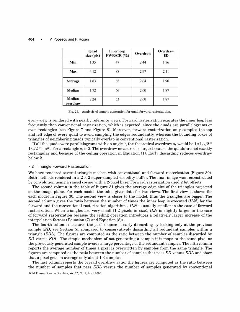
404 • V. Popescu and P. Rosen
Fig. 29. Analysis of sample generation for quad forward rasterization.
every view is rendered with nearby reference views. Forward rasterization executes the inner loop lessfrequently than conventional rasterization, which is expected, since the quads are parallelograms oreven rectangles (see Figure 7 and Figure 8). Moreover, forward rasterization only samples the topand left edge of every quad to avoid sampling the edges redundantly, whereas the bounding boxes oftriangles of neighboring quads typically overlap in conventional rasterization.
If all the quads were parallelograms with an angle θ , the theoretical overdraw ot would be 1/(1/√
2 *1/
√2 * sinθ ). For a rectangle ot is 2. The overdraw measured is larger because the quads are not exactly
rectangular and because of the ceiling operation in Equation (1). Early discarding reduces overdrawbelow 2.
7.2 Triangle Forward Rasterization
We have rendered several triangle meshes with conventional and forward rasterization (Figure 30).Both methods rendered in a 2 × 2 super-sampled visibility buffer. The final image was reconstructedby convolution using a raised cosine with a 2-pixel base. Forward rasterization used 2 bit offsets.
The second column in the table of Figure 31 gives the average edge size of the triangles projectedon the image plane. For each model, the table gives data for two views. The first view is shown foreach model in Figure 30. The second view is closer to the model, thus the triangles are bigger. Thesecond column gives the ratio between the number of times the inner loop is executed (ILN) for theforward and the conventional rasterization algorithms. ILN is usually smaller in the case of forwardrasterization. When triangles are very small (1.2 pixels in size), ILN is slightly larger in the caseof forward rasterization because the ceiling operation introduces a relatively larger increase of theinterpolation factors (Equation (7) and Equation (8)).
The fourth column measures the performance of early discarding by looking only at the previoussample (ED, see Section 5), compared to conservatively discarding all redundant samples within atriangle (EDL). The figures are computed as the ratio between the number of samples discarded byED versus EDL. The simple mechanism of not generating a sample if it maps to the same pixel asthe previously generated sample avoids a large percentage of the redundant samples. The fifth columnreports the average number of times a pixel is overwritten by samples from the same triangle. Thefigures are computed as the ratio between the number of samples that pass ED versus EDL and showthat a pixel gets on average only about 1.3 samples.
The last column reports the overall overdraw ratio; the figures are computed as the ratio betweenthe number of samples that pass EDL versus the number of samples generated by conventional
ACM Transactions on Graphics, Vol. 25, No. 2, April 2006.
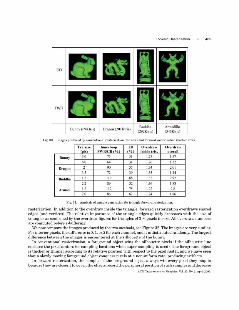
Forward Rasterization • 405
Fig. 30. Images produced by conventional rasterization (top row) and forward rasterization (bottom row).
Fig. 31. Analysis of sample generation for triangle forward rasterization.
rasterization. In addition to the overdraw inside the triangle, forward rasterization overdraws sharededges (and vertices). The relative importance of the triangle edges quickly decreases with the size oftriangles as confirmed by the overdraw figures for triangles of 3–6 pixels in size. All overdraw numbersare computed before z-buffering.
We now compare the images produced by the two methods, see Figure 32. The images are very similar.For interior pixels, the difference is 0, 1, or 2 for each channel, and it is distributed randomly. The largestdifference between the images is encountered at the silhouette of the bunny.
In conventional rasterization, a foreground object wins the silhouette pixels if the silhouette lineencloses the pixel centers (or sampling locations when super-sampling is used). The foreground objectis thicker or thinner according to its relative position with respect to the pixel raster, and we have seenthat a slowly moving foreground object conquers pixels at a nonuniform rate, producing artifacts.
In forward rasterization, the samples of the foreground object always win every pixel they map tobecause they are closer. However, the offsets record the peripheral position of such samples and decrease
ACM Transactions on Graphics, Vol. 25, No. 2, April 2006.
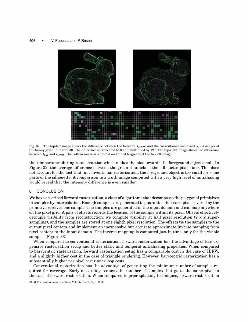
406 • V. Popescu and P. Rosen
Fig. 32. The top-left image shows the difference between the forward (IFWR) and the conventional rasterized (ICR) images of
the bunny given in Figure 30. The difference is truncated to 0 and multiplied by 127. The top-right image shows the difference
between ICR and IFWR. The bottom image is a 16-fold magnified fragment of the top left image.
their importance during reconstruction which makes the bias towards the foreground object small. InFigure 32, the average difference between the green channels of the silhouette pixels is 9. This doesnot account for the fact that, in conventional rasterization, the foreground object is too small for someparts of the silhouette. A comparison to a truth image computed with a very high level of antialiasingwould reveal that the intensity difference is even smaller.
8. CONCLUSION
We have described forward rasterization, a class of algorithms that decomposes the polygonal primitivesin samples by interpolation. Enough samples are generated to guarantee that each pixel covered by theprimitive receives one sample. The samples are generated in the input domain and can map anywhereon the pixel grid. A pair of offsets records the location of the sample within its pixel. Offsets effectivelydecouple visibility from reconstruction: we compute visibility at half pixel resolution (2 × 2 super-sampling), and the samples are stored at one eighth pixel resolution. The offsets tie the samples to theoutput pixel centers and implement an inexpensive but accurate approximate inverse mapping frompixel centers to the input domain. The inverse mapping is computed just in time, only for the visiblesamples (Figure 33).
When compared to conventional rasterization, forward rasterization has the advantage of less ex-pensive rasterization setup and better static and temporal antialiasing properties. When comparedto barycentric rasterization, forward rasterization setup has a comparable cost in the case of IBRW,and a slightly higher cost in the case of triangle rendering. However, barycentric rasterization has asubstantially higher per pixel cost (inner loop cost).
Conventional rasterization has the advantage of generating the minimum number of samples re-quired for coverage. Early discarding reduces the number of samples that go to the same pixel inthe case of forward rasterization. When compared to prior splatting techniques, forward rasterization
ACM Transactions on Graphics, Vol. 25, No. 2, April 2006.
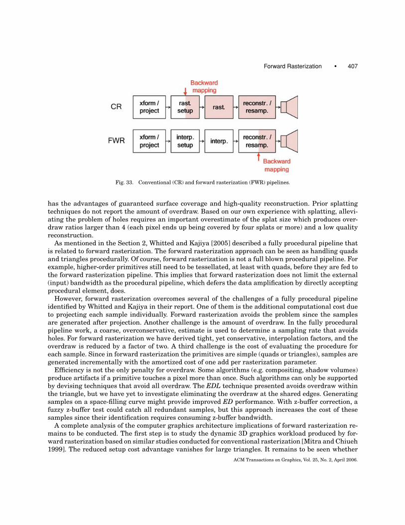
Forward Rasterization • 407
Fig. 33. Conventional (CR) and forward rasterization (FWR) pipelines.
has the advantages of guaranteed surface coverage and high-quality reconstruction. Prior splattingtechniques do not report the amount of overdraw. Based on our own experience with splatting, allevi-ating the problem of holes requires an important overestimate of the splat size which produces over-draw ratios larger than 4 (each pixel ends up being covered by four splats or more) and a low qualityreconstruction.
As mentioned in the Section 2, Whitted and Kajiya [2005] described a fully procedural pipeline thatis related to forward rasterization. The forward rasterization approach can be seen as handling quadsand triangles procedurally. Of course, forward rasterization is not a full blown procedural pipeline. Forexample, higher-order primitives still need to be tessellated, at least with quads, before they are fed tothe forward rasterization pipeline. This implies that forward rasterization does not limit the external(input) bandwidth as the procedural pipeline, which defers the data amplification by directly acceptingprocedural element, does.
However, forward rasterization overcomes several of the challenges of a fully procedural pipelineidentified by Whitted and Kajiya in their report. One of them is the additional computational cost dueto projecting each sample individually. Forward rasterization avoids the problem since the samplesare generated after projection. Another challenge is the amount of overdraw. In the fully proceduralpipeline work, a coarse, overconservative, estimate is used to determine a sampling rate that avoidsholes. For forward rasterization we have derived tight, yet conservative, interpolation factors, and theoverdraw is reduced by a factor of two. A third challenge is the cost of evaluating the procedure foreach sample. Since in forward rasterization the primitives are simple (quads or triangles), samples aregenerated incrementally with the amortized cost of one add per rasterization parameter.
Efficiency is not the only penalty for overdraw. Some algorithms (e.g. compositing, shadow volumes)produce artifacts if a primitive touches a pixel more than once. Such algorithms can only be supportedby devising techniques that avoid all overdraw. The EDL technique presented avoids overdraw withinthe triangle, but we have yet to investigate eliminating the overdraw at the shared edges. Generatingsamples on a space-filling curve might provide improved ED performance. With z-buffer correction, afuzzy z-buffer test could catch all redundant samples, but this approach increases the cost of thesesamples since their identification requires consuming z-buffer bandwidth.
A complete analysis of the computer graphics architecture implications of forward rasterization re-mains to be conducted. The first step is to study the dynamic 3D graphics workload produced by for-ward rasterization based on similar studies conducted for conventional rasterization [Mitra and Chiueh1999]. The reduced setup cost advantage vanishes for large triangles. It remains to be seen whether
ACM Transactions on Graphics, Vol. 25, No. 2, April 2006.
408 • V. Popescu and P. Rosen
in this case the static and temporal antialiasing advantages are sufficient to offset the additional costintroduced by the redundant samples. We will investigate subdividing large triangles 50 as to minimizethe number of redundant samples. We will design a coarse rasterizer best suited for forward rasteriza-tion, similar to the ones used in conventional rasterization, to break up large triangles in rectangulartiles and left-over triangles.
The cost analysis presented here focuses on computational cost. The bandwidth requirement is animportant component of the total cost of an algorithm and an important factor when deciding its suit-ability for hardware implementation. The number of interpolants and the number of samples generatedbegin to outline the bandwidth requirements for forward rasterization. However, a detailed analysisof these requirements is still in the future as it is tied to actually devising a hardware architecturethat implements forward rasterization. Our method will be compared again to other rasterization al-gorithms under this new angle. Barycentric interpolation, for example, trades computational cost (chiparea) for a reduction of the bandwidth between the rasterizers and the fragment units.
Also as future work, we will perform a signal processing analysis of forward rasterization and at-tempt to design a reconstruction kernel optimized for offset reconstruction that will eliminate the smalldifference between the 16 × 16 offset reconstruction and the truth graphs in Figure 18.
Important future work will adapt texture mip-mapping and level of detail to forward rasterization.An option is to restrict the possible interpolation factors f1 and f2 to values that are power of two, andto store mipmaps based on these fixed values. Another important extension which will increase the us-ability of forward rasterization in the context of today’s Graphics hardware is support for multisamplingas a cost effective alternative to super-sampling.
Forward rasterization can readily replace conventional rasterization to provide infrastructure sup-port for higher-level computer graphics algorithms. Offset reconstruction offers independence from thepixel grid. The technique could be used to avoid resampling errors whenever an intermediate sample-based representation is constructed (e.g. LDIs, acceleration by repeated reprojection of prerenderedsamples). Another possible use that we will investigate is to optimize sampling. For example, geom-etry images [Gu et al. 1992] augmented with a vertex per pixel that is freely placed within the pixelboundaries have increased modeling power that comes at a small additional cost.
APPENDIX 1
Sample generation algorithm for forward rasterization of triangles. The triangle vertices project at V0,V1, and V2. The samples generated are illustrated in Figure 13.
For each of three possible pairs of edges (V i0 V i
1 , V i0 V i
2 )
If V i0 V i
1 and V i0 V i
2 are in same quadrant compute ( f i0 , f i
1) with Equation 7
Else compute ( f i0 , f i
1)with Equation 8.EndForChoose pair of edges with smallest f0 f1 product; let that be (V0V1, V0V2).uLine = u0; duLine = (u1 − u0)/ f0; vLine = v0; dvLine = (v1 − v0)/ f0;samplesN = f1+ 1; dsamplesNLine = f1/ f0;du = (u2 − u0)/ f1; dv = (v2 − v0)/ f1;For lineIndex = 0 to f0
u = uLine; v = vLine;For sampleIndex = 0 to samplesN
UseSample(u, v);u +=du;v +=dv;
EndForu = u2+ lineIndex/f0 ∗ (u1 − u2), v = v2+ lineIndex/f0 ∗ (v1 − v2);
ACM Transactions on Graphics, Vol. 25, No. 2, April 2006.
Forward Rasterization • 409
UseSample(u, v)samplesN = floor(samplesN – lineIndex*dsamplesNLine);uLine = uLine + lineIndex*duLine; vLine = vLine + lineIndex*dvLine;
EndFor
ACKNOWLEDGMENTS
The authors are grateful to John Eyles, Anselmo Lastra, Gary Bishop, Joshua Steinhurst, Nick England,Lars Nyland, John Poulton, and Chris Hoffmann for numerous fruitful discussions. We thank JohnOwens for promptly providing reviewers and a hard to find technical report. The anonymous reviewers,the associate editor, and the editor in chief have generously donated many hours of their time towardsimproving this manuscript, for which we thank them sincerely.
REFERENCES
ABRAM, G. AND WESTOVER, L. 1985. Efficient alias-free rendering using bit-masks and look-up tables. In Proceeding ofSIGGRAPH. 53–59.
AKELEY, K. 1993. RealityEngine Graphics. In Proceedings of SIGGRAPH. 109–116.
ALIAGA, D. AND LASTRA, A. 1999. Automatic image placement to provide a guaranteed frame rate. In Proceedings of SIGGRAPH.
307–316.
ATI. http://www.ati.com.
BROWN, R. 1999a. Barycentric coordinates as interpolants. Sun Microsystems Tech. rep.
BROWN, R. 1999b. Modeling specular highlights using bezier triangles. Sun Microsystems Tech. rep.
CARPENTER, L. 1984. The A-Buffer, an antialiased hidden surface method. In Proceedings of SIGGRAPH. 103–108.
CHANG, C., BISHOP, G., AND LASTRA, A. 1999. LDI Tree: A hierarchical representation for image-based rendering. In Proceedingsof SIGGRAPH. 291–298.
COOK, R. 1986. Stochastic sampling in computer graphics. ACM Trans. Graph. 5, 1, 51–72.
COOK, R., CARPENTER, L., AND CATMULL, E. 1987. The Reyes image rendering architecture. In Proceedings of the 14th AnnualConference on Computer Graphics and Interactive Techniques. 95–102.
DEERING, M. AND NAEGLE, D. 2002. The SAGE graphics architecture. In Proceedings of SIGGRAPH. 683–692.
MICROSOFT DIRECTX, MULTIMEDIA API. http://www.microsoft.com/windows/directx/default.aspx
DUGUET, F. AND DRETTAKIS, G. 2004. Flexible point-based rendering on mobile devices. Point-Based Comput. Graph. 57–63.
ELLSWORTH, D. 1996. Polygon rendering for interactive visualization on multicomputers. Ph.D. Dissertation, Computer Science
Department, University of North Carolina at Chapel Hill, NC.
EYLES, J., MOLNAR, S., POULTON, J., GREER, T., LASTRA, A., ENGLAND, N., AND WESTOVER, L. 1997. PixelFlow: The realization. In
Proceedings of the SIGGRAPH/EUROGRAPHICS Workshop on Graphics Hardware. 57–68.
FUCHS, H., GOLDFEATHER, J., HULTQUIST, J., SPACH, S., AUSTIN, J., BROOKS, F., EYLES, J., AND POULTON, J. 1985. Fast spheres, shadows,
textures, transparencies, and image enhancements in pixel-planes. In Proceedings of SIGGRAPH. 111–120.
FUCHS, H., POULTON, J., EYLES, J., GREER, T., GOLDFEATHER, J., ELLSWORTH, D., MOLNAR, S., TURK, G., TEBBS, B., AND ISRAEL, L. 1989.
Pixel-Planes 5: A heterogeneous multiprocessor graphics system using processor-enhanced memories. In Proceedings of SIG-GRAPH. 79–88.
GARACHORLOO, N., SPROULL, R. F., GUPTA, G., AND SUTHERLAND, I. 1989. A characterization of ten rasterization techniques. In
Proceedings of SIGGRAPH. 355–368.
GLASSNER, A. 1978. An Introduction to Ray-Tracing. The Morgan Kauffman Series in Computer Graphics.
GREENE, N. 1996. Hierarchical polygon tiling with coverage masks. In Proceedings of SIGGRAPH. 65–74.
GU, X., GORTLER, S., AND HOPPE, H. 2002. Geometry images. In Procedings of the SIGGRAPH. 355–361.
HAEBERLI, P. 1990. Paint by numbers: Abstract image representations. In Proceedings of SIGGRAPH. 207–214.
HECKBERT, P. 1989. Fundamentals of texture mapping and image warping. Master’s thesis, Department of Electrical Engineer-
ing and Computer Science, University of California at Berkeley.
KAUFMAN, A. 1993. Rendering, Visualization, and Rasterization Hardware. Springer-Verlag, New York, NY.
LARSON, G. 1998. The Holodeck: A parallel ray-caching system. In Proceedings of Eurographics Workshop on Parallel Graphicsand Visualization.
ACM Transactions on Graphics, Vol. 25, No. 2, April 2006.
410 • V. Popescu and P. Rosen
LEVOY, M. AND WHITTED, T. 1985. The use of points as a display primitive. UNC Computer Science Tech. rep. TR85-022.
MARK, W., MCMILLAN, L., AND BISHOP, G. 1997. Post-rendering 3D warping. Symposium on Interactive 3D Graphics. 7–
16.
MARK, W. 1999. Post-rendering 3D image warping: Visibility, reconstruction, and performance for depth-image warping. Ph.D.
Thesis, University of North Carolina at Chapel Hill, NC.
MCALLISTER, D., NYLAND, L., POPESCU, V., LASTRA, A., AND MCCUE, C. 1999. Real-time rendering of real-world environments. In
Proceedings of Eurographics Workshop on Rendering. 145–160.
MCCOOL, M., WALES, C., AND MOULE, K. 2001. Incremental and hierarchical hilbert order edge equation polygon rasterization.
In Proceedings of ACM/Eurographics Symposium on Graphics Hardware.
MCCORMACK, J. AND MCNAMARA, R. 2000. Tiled polygon traversal using half-plane edge functions. In Proceedings of the ACMSIGGRAPH/Eurographics Workshop on Graphics Hardware. 15–21.
MCMILLAN, L. AND BISHOP, G. 1995. Plenoptic modeling: An image-based rendering system. In Proceedings of SIGGRAPH.
39–46.
MCMILLAN, L. 1997. An image-based approach to three-dimensional computer graphics. Ph.D. Thesis, University of North
Carolina at Chapel Hill, NC.
MITRA, T. AND CHIUEH, T. 1999. Dynamic 3D graphics workload characterization and the architectural implications. In Pro-ceedings of the 32nd Annual ACM/IEEE International Symposium on Microarchitecture. 62–71.
MOLNAR, S., EYLES, J., AND POULTON, J. 1992. PixelFlow: High-speed rendering using image composition. In Proceedings ofSIGGRAPH. 231–240.
MOLNAR, S. 1991. Efficient supersampling antialiasing for high-performance architectures. UNC-CS Tech. rep. TR91-023.
MONTRYM J., BAUM, D., DIGNAM, D., AND MIGDAL, C. 1997. InfiniteReality: A real-time graphics systems. In Proceedings ofSIGGRAPH. 293–302.
NVIDIA. http://www.nvidia.com.
BURROWS ET AL. 2004. All about antialiasing. NVIDIA whitepaper. http://www.nvidia.com/object/all about aa.html.
NVIDIA. 2005A. ACCUVIEW TECHNOLOGY. NVIDIA tech. brief. http://www.nvidia.com/object/feature accuview.html.
NVIDIA. 2005b. High-Resolution Antialiasing Through Multisampling. NVIDIA tech. brief. http://www.nvidia.com/object/
feature hraa. html.
OLANO, M. 1998. A programmable pipeline for graphics hardware. Ph.D. Thesis, Department of Computer Science, The Uni-
versity of North Carolina at Chapel Hill, NC.
OLANO, M. AND GREER, T. 1997. Triangle scan conversion using 2D homogeneous coordinates. In Proceedings ofACM/Eurographics Symposium on Graphics Hardware. 89–95.
OPENGL. Computer graphics API. http://www.opengl.org/.
OWENS, J. 2003. Computer graphics on a stream architecture. Ph.D. thesis, Computer Science Department, Stanford University.
PFISTER, H., ZWICKER, M., VAN BAAR, J., AND GROSS, M. 2000. Surfels: Surface elements as rendering primitives. In Proceedingsof SIGGRAPH. 335–342.
PINEDA, J. 1988. A parallel algorithm for polygon rasterization. ACM Proceedings of the 15th Annual Conference on Computer
Graphics and Interactive Techniques. vol. 22, 4, 17–20.
POPESCU, V., LASTRA, A., ALIAGA, D., AND OLIVEIRA, M. 1998. Efficient warping for architectural walkthroughs using layered
depth images. In Proceedings of IEEE Visualization. 211–215.
POPESCU, V., EYLES, J., LASTRA, A., STEINHURST, J., ENGLAND, N., AND NYLAND, L. 2000. The WarpEngine: An architecture for the
post-polygonal age. In Proceedings of SIGGRAPH. 433–442.
POPESCU, V. 2001. Forward Rasterization: A reconstruction algorithm for image-based rendering. Ph.D. thesis, Computer
Science Department, University of North Carolina at Chapel Hill, NC.
RAFFERTY, M., ALIAGA, D., AND LASTRA, A. 1998. 3D image warping in architectural walkthroughs. In Proceedings of VRAIS.
228–233.
REN, L., PFISTER, H., AND ZWICKER, M. 2002. Object space EWA surface splatting: A hardware accelerated approach to high
quality point rendering. In Proceedings EUROGRAPHICS, 461–470.
RUSINKIEWICZ, S. AND LEVOY, M. 2000. QSplat: A multiresolution point rendering system for large meshes. In Proceedings ofSIGGRAPH, 343–352.
SCHILLING, A. 1991. A new simple and efficient antialiasing with subpixel masks. In Proceedings of SIGGRAPH, 133–141.
SHADE, J., GORTLER, S., HE, L., AND SZELISKI, R. 1998. Layered depth images. In Proceedings of SIGGRAPH, 231–242.
WESTOVER, L. 1990. Footprint evaluation for volume rendering. In Proceedings of SIGGRAPH, 367–376.
ACM Transactions on Graphics, Vol. 25, No. 2, April 2006.
Forward Rasterization • 411
WHITTED, T. AND KAJIYA, J. 2005. Fully procedural graphics. In Proceedings of the ACM SIGGRAPH/EUROGRAPHICS Con-ference on Graphics Hardware, 81–90.
WHITTED, T. AND WEIMER, D. 1982. A software testbed for the development of 3D raster graphics systems. ACM Trans. Graph.1, 43–58.
ZWICKER, M., PFISTER, H., VAN BAAR, J., AND GROSS, M. 2002. EWA splatting. IEEE Trans. Visualiz. Comput. Graph. 223–238.
Received April 2005; revised October and November 2005; accepted December 2005
ACM Transactions on Graphics, Vol. 25, No. 2, April 2006.