Embed Size (px)
Citation preview

Forward Looking Estimates of Interest Rate
Distributions ∗
Jonathan H. Wright†
First Version: July 12, 2016This version: August 29, 2016
Abstract
This paper reviews methods for extracting both risk-neutral and physical den-sity forecasts for interest rates. It presents some applications, with particularfocus on issues pertaining to forward guidance and the zero lower bound. Sev-eral important applied questions in macroeconomics and monetary economicscan be very directly addressed using the wealth of information in interest ratederivative securities.
Keywords: Density Forecasting, Interest Rates, Options, Risk Premia, Zero LowerBound.JEL Classification: C53, E43, G12.
DRAFT PREPARED FOR THE ANNUAL REVIEW OF FINANCIALECONOMICS
∗I am grateful to Tobias Adrian for helpful comments on an earlier draft. All errors and omissionsare my sole responsibility.†Department of Economics, Johns Hopkins University, Baltimore MD 21218; [email protected].

1 Introduction
Central banks, academics and the press routinely use the yield curve to measure
expectations of the future path of interest rates, although they are increasingly aware
that the task is complicated by the presence of time-varying term premia (Shiller,
Campbell, and Schoenholtz, 1983; Kim and Wright, 2005; Cochrane and Piazzesi,
2005; Adrian, Crump, and Moench, 2013). But much more can be done. Financial
asset prices help us to measure uncertainty about future interest rates and higher
moments—in fact, they can give us entire probability density functions, although
these are again complicated by risk premia. The technology for forward-looking
estimates of interest rate distributions is well established in the finance literature,
but is underutilized by monetary and macroeconomists. It can, in particular, be used
to answer questions about the efficacy of forward guidance and the probability of
being at the zero lower bound, or of negative interest rates, at dates in the future. It
can be used to assess how the zero lower bound affects longer-term interest rates.
This paper reviews methods for constructing forward looking estimates of interest
rate distributions. I will consider the distributions implied by the prices of options
and other derivatives. These give the state price densities, i.e. distributions under
the risk neutral, or more precisely, under the forward measure. Their interpretation
is complicated by the presence of risk premia. I will also consider methods to con-
struct physical density forecasts. Given the availability of actively traded interest
rate derivatives, risk-neutral pdfs for future nominal interest rates can be constructed
day-by-day with minimal modeling assumptions and negligible measurement error.
Alas, it is not so easy for the physical density forecasts. These are normally con-
structed based on historical time series patterns of interest rates, and are plagued
by model and parameter uncertainty and by structural instability. In limited cases,
surveys provide an alternative source of information on physical density forecasts,
that do not suffer from these problems.
The plan for the remainder of this paper is as follows. In section 2, I review
methods of constructing risk-neutral pdfs. This is a brief review of an enormous
literature—far more comprehensive treatments from a finance practitioner’s perspec-
tive are available in Rebonato (2003) and Brigo and Mercurio (2006). In section 3, I
turn to physical density forecasts, and discuss the pricing kernel that links the risk-
neutral and physical densities. Section 4 applies the methods to Eurodollar options
1
and other interest rate derivatives over recent years, with particular emphasis on ques-
tions pertaining to the zero lower bound (ZLB). This section is intended to highlight
the potential uses of the techniques discussed in this paper in macroeconomics and
central banking. Section 5 concludes.
2 Risk-neutral pdfs
Define Pt(n) as the price at time t of a n-period zero coupon bond that pays $1 at
time t+ n and let yt(n) = − 1n
log(Pt(n)) denote its yield. Let
ft(n1, n2) =(n2 − t)yt(n2 − t)− (n1 − t)yt(n1 − t)
n2 − n1
(2.1)
denote a forward interest rate from time n1 to time n2 (t ≤ n1 < n2).
Suppose that we have options with payoffs that are tied to yτ (n) an n-period
interest rate at time τ ≥ t. The payoffs are
max(yτ (n)−K, 0) (2.2)
for different choices of the strike price K. For example, if n is 3 months, this corre-
sponds to a Eurodollar option that is based on a three-month LIBOR interest rate1.
The valuation of this asset at time t is:
Et(M(t, τ) max(yτ (n)−K, 0)) (2.3)
where Et denotes the physical expectation and M(t1, t2) is the pricing kernel from
time t1 to time t2. The valuation can alternatively be written as:
Pt(τ − t)E∗t (max(yτ (n)−K, 0)) (2.4)
1Strictly, Eurodollar options settle not to the interest rate but to 100 minus the interest rate. Acall/put Eurodollar option is a bet on falling/rising interest rates, respectively. But we can think ofthem as derivatives with payoffs of the form of equation (2.2).
2

where E∗t denotes the expectation under the forward risk-neutral measure2. Hence-
forth, I refer to the forward risk-neutral measure as the risk-neutral measure, or
Q-measure. The objective is to reverse-engineer the Q-measure probability density
for the future interest rate yτ (n) from the observed price of the options.
2.1 Other derivatives
Many more interest rate derivatives exist, but these can all be priced using the same
principles. Here is a list of some of the most important, that are discussed in much
depth in references including Brigo and Mercurio (2006) and Veronesi (2010).
1. Interest rate caps are contracts that at various future dates pay the amount that
the interest rate exceeds a strike price on a notional underlying principal if the
interest rate exceeds that strike price, and zero otherwise. These are effectively
bundles of call options on the interest rate, with payoffs of the form in equation
(2.2).
2. Options on Treasury futures confer the right, but not the obligation, to enter
into a Treasury futures contract. They are traded on the CME and are American
options (early exercise is possible). Treasury futures contracts are complicated,
but are structured in such a way that a long position in a Treasury futures
contract can be roughly thought of as a contract to buy the shortest maturity
security in the delivery basket3, and so the futures option is approximately an
option on that security. The MOVE index is an index of implied volatilities
on two-, five-, ten- and thirty- year Treasury futures contracts, constructed by
Merrill Lynch, and is the equivalent of the VIX for interest rate uncertainty.
Since 2011, the CME has traded options on Treasury futures that expire each
Friday afternoon4. Though new, they are quite liquid, and can be used to
2The valuation of the security under the ordinary risk-neutral measure would be the expectationof exp(−
∫ t+τt
r(s)ds) max(yτ (n)−K, 0) where r(s) is the instantaneous interest rate. The discount
factor exp(−∫ t+τt
r(s)ds) is random and cannot be pulled through the expectations operator. Theforward risk-neutral measure (Jamshidian, 2007; Jarrow, Li, and Zhao, 2007; Li and Zhao, 2009)instead takes the (τ − t)-period zero coupon bond as the numeraire, which is known at time t andso can be pulled outside the expectations operator.
3This statement is true for US Treasury futures so long as the level of interest rates is below 6percent, which has been true for a very long time.
4The holder must enter into a futures position by the expiration day, or else the option expiresunused.
3

measure uncertainty about specific risk events, like employment reports (Kim
and Wright, 2014).
3. A payer swaption gives the holder the right, but not the obligation, to enter
into a swap contract where they pay a particular fixed rate. A receiver swap-
tion gives the holder the right, but not the obligation, to enter a swap contract
where they receive a particular fixed rate. Swaptions are typically European5.
If the swaption expires at time τ and the underlying swap contract calls for
R payments every ∆ years on a notional underlying principal of L, if the swap-
tion has a strike price of iS and if the swap rate at expiration is iF , then the
value of a receiver swaption at expiration is L∆ max(iF−iS, 0)ΣRi=1Pτ (i∆) which
is a rescaled version of the payoff in equation (2.2).
2.2 Black Model
For an option with the payoffs in equation(2.2), a simple approach to reverse-engineering
the risk-neutral pdf is to posit that the forward rate ft(τ, τ + n) follows the following
process under the Q-measure:
dft(τ, τ + n)
ft(τ, τ + n)= σdWt (2.5)
where Wt is a standard Brownian motion. Noting that fτ (τ, τ +n) = yτ (n), it follows
using Ito’s lemma that:
log yτ (n) ∼ N(log(ft(τ, τ + n))− 1
2σ2τ ∗, σ2τ ∗) (2.6)
where τ ∗ = τ − t is the time to maturity. Under this premise, Black (1976) gives an
analytical expression for equation (2.4) at time t. Given the price of a single option,
this can be inverted to obtain the implied volatility, σ. A 95% confidence interval for
yτ (n) can then be constructed as:
[ft(τ, τ + n) exp(−1
2σ2τ ∗ − 1.96σ
√τ ∗), ft(τ, τ + n) exp(−1
2σ2τ ∗ + 1.96σ
√τ ∗)] (2.7)
The implied volatility in equation (2.5) is not directly a measure of uncertainty about
5Bermudan swaptions are also quite common. A Bermudan swaption can be exercised on certainspecified dates only.
4

the level of interest rates. Uncertainty about the level of interest rates can be mea-
sured by the width of a 95% confidence interval for yτ (n), which is:
ft(τ, τ + n) exp(−1
2σ2τ ∗)[exp(1.96σ
√τ ∗)− exp(−1.96σ
√τ ∗)] (2.8)
The assumption in equation (2.5) implies that interest rates can never go negative.
Until recently, this seemed quite uncontroversial. But many benchmark interest rates
are negative today, and that cannot be accommodated in this framework. There is an
alternative version of the Black formula that assumes that forward rates are normal,
not lognormal, and that will allow interest rates to go negative. Much more on the
zero lower bound and negative interest rates below.
2.3 BGM Model
An extension of the Black (1976) model entails specifying that a vector of forward
rates (f(τ1, τ1 + n), f(τ2, τ2 + n)...f(τK , τK + n))′ follows a multivariate geometric
Brownian motion with variance-covariance matrix V (t) = [vij(t)]. This is known as
the BGM model (Brace, Gatarek, and Musiela, 1997), or the LIBOR market model.
The variance-covariance matrix can in turn be specified to depend on a smaller number
of parameters—a common parameterization (Rebonato, 1999) is:
vij(t) = σi(t)σj(t) exp(−β|i− j|) (2.9)
where
σi(t) = (a(τi − t) + b) exp(−c(τi − t)) + d (2.10)
This constrains V (t) to depend only on five parameters. These parameters can be
estimated by minimizing the sum of squared deviations between actual and model-
implied interest rate derivatives prices. Having obtained the entire joint risk-neutral
distribution of forward rates, the researcher can work out the implied density of many
objects of interest, such as the timing of the peak of a tightening cycle. Elliott and
Noss (2015) discuss applying the BGM model for such purposes. I will illustrate this
5
use of the model in section 4, below6.
The BGM model is closely related to the well-known HJM model (Heath, Jar-
row, and Morton, 1992). The difference is that Heath, Jarrow, and Morton (1992)
consider a law of motion for instantaneous forward rates. Unfortunately, it turns
out that lognormal instantaneous forward rates are inconsistent with an absence of
arbitrage. For this reason, the BGM model retains the HJM framework but replaces
instantaneous forward rates with discretely compounded forward rates, which have
the useful by-product of being of more direct relevance to market participants, as
actual market rates all have discrete accrual periods. Sandmann and Sondermann
(1997), Goldys, Musiela, and Sondermann (2000), Jarrow (2009) and Shreve (2004)7
all discuss this motivation for using discretely compounded forward rates. Essentially,
the BGM model can be thought of as a device that circumvents a technical problem
of explosive rates in the HJM model.
2.4 PDFs at a given point in time
Another approach is to collect a set of option prices for a fixed maturity date and
to reverse-engineer a pdf for yt(n) from these prices without making any parametric
assumptions. The key insight in doing this is the result of Breeden and Litzenberger
(1978) that if C(K) is the price of a call option at a strike price of K on a future
interest rate yτ (n), then the cumulative distribution function of yτ (n) is
F (x) = − 1
P (t, t+ τ)
∂C(x)
∂K(2.11)
and the probability density function is
f(x) =1
P (t, t+ τ)
∂2C(x)
∂K2(2.12)
We do not observe options at every strike price, and so cannot literally compute
the derivatives required for these equations. But we can work out the Black-implied
6A different approach, that also gives a researcher the joint risk-neutral distribution of futureshort term interest rates is to calibrate models of short-term interest rates, such as the Hull andWhite (1990) one-factor model, or the Longstaff and Schwartz (1992) two-factor model, to interestrate derivatives prices. I do not consider this further in the current paper, but Rebonato (2003) andBrigo and Mercurio (2006) give extensive discussion of these methods.
7See subsection 10.4.1 of this reference for a textbook treatment.
6

volatility for each option, interpolate these implied volatilities over an arbitrarily fine
grid of points, convert these back into call prices, and then compute the required
derivatives numerically. This approach is implemented by Shimko (1993) and Bliss
and Panigirtzoglou (2002). Shimko (1993) uses a polynomial in K to smooth the
implied volatilities, whereas Bliss and Panigirtzoglou (2002) use a cubic spline. In
Monte-Carlo simulations, Bliss and Panigirtzoglou (2002) find that this method is
reliable even with quite a small numbers of options.
Another related approach is the local linear regression of Aıt-Sahalia and Duarte
(2003). Consider a set of L call options at different strike prices at a given point in
time for the same underlying asset. Let Ci denote the price of the ith option, with a
strike of ki. We seek to approximate the price of an option at a strike price k′ in a
neighborhood around k by a locally linear function β0(k)+β1(k)(k′−k). We estimate
the coefficients as:
β0(k), β1(k) = arg minβ0(k),β1(k),β2(k)
ΣLi=1{Ci−β0(k)−β1(k)(ki−k)}2K(
ki − kh
)/h, (2.13)
where K(.) is a kernel function and h is a bandwidth. There are expressions for the
optimal bandwidth in terms of minimizing integrated mean squared error, but it is
always wise to look at the smoothed option price to visually judge if the degree of
smoothing is appropriate. The first derivative of the call option price with respect
to the strike price can then be obtained as β1(k) and the second derivative can be
obtained as β′1(k).
A variant on this approach—discussed in Aıt-Sahalia and Duarte (2003)—is to
approximate the price of the option by a locally quadratic function. The second
derivative can then be recovered directly from the coefficient on the quadratic term.
However, inferring the second derivative from equation (2.13) may work better in
finite samples (Aıt-Sahalia and Duarte, 2003).
2.5 PDFs smoothed over time
In the previous section, we considered constructing a pdf on a given day, or at a
particular point in time. This can be appealing because one can then study how
a unique event, such as the introduction of some type of forward guidance by the
Fed, shifted the pdf. However, because of concerns about measurement error or the
absence of options at the required maturity and strike price, it may be preferable to
7
pool options prices over a longer period of time. Such an approach is proposed in
the semiparametric methodology of Aıt-Sahalia and Lo (1998).
In this approach, observed options prices are converted into Black implied volatil-
ities. Let these options implied volatilities be {σi}ni=1, where n is the total number of
options, pooling all call and put options on all trading days, strike prices and expira-
tion dates. Assume that the implied volatility is a function of a state vector, σ(Zit),
where the state vector, Zit, includes the strike price or moneyness of the option, the
maturity of the option, and time-varying variables such as the level and slope of the
term structure and/or the options implied volatility of interest rates. The implied
volatility function can be estimated nonparametrically by kernel smoothing or by a
local linear regression. Implied volatilities can then be converted back to call options
prices and fitted call options prices can be constructed for any value of the state
vector, giving the Q-measure cdf and pdf in equations (2.11) and (2.12). Intuitively,
the value of an option on a given day is constructed by smoothing over options with
similar strike prices and maturities and over days when the state vector takes on
similar values. The advantage of doing this is that the estimation of the state price
density can be made much more precise. The disadvantage is that we have to assume
that a low dimensional state vector provides a good fit to implied volatilities, though
of course this is an assumption that can be checked by seeing how well the fitted
implied volatilities match their actual counterparts. Li and Zhao (2009) apply this
methodology to LIBOR derivatives; more recently Wright (forthcoming) applies it to
a new but thin market on exchange-traded options on Treasury Inflation Protected
Securities (TIPS).
3 Physical density forecasts
There is a large literature on forecasting interest rates, with a recent comprehensive
summary in Duffee (2013). Most of the emphasis in this literature is on point forecast-
ing. As is well known, nearly all variation in yields reduces to variation in three factors
(Litterman and Scheinkman, 1991). These are the first three principal components
of yields that can be interpreted as level, slope and curvature, or are equivalently (up
to a rotation) the three coefficients in the Nelson and Siegel (1987) model. Most of
the point forecasts for interest rates that are used in the literature amount to using a
possibly restricted vector autoregression in these three factors to predict future values
8

of the factors, that in turn imply forecasts of future interest rates. Diebold and Li
(2006) propose a dynamic Nelson-Siegel model (Nelson and Siegel, 1987), fitting an
AR(1) to each of the Nelson-Siegel coefficients. This is a good benchmark for interest
rate forecasting, though it should be noted that the record of this and other meth-
ods for interest rate forecasting in out-of-sample prediction exercises is sensitive to
the period used for forecast evaluation, and the very simplest forecasting model—a
random walk forecast—is hard to beat consistently (Duffee, 2013).
In this article, my focus is on density forecasting, not point forecasting. In line
with standard terminology, I refer to the physical density forecast as the P-measure
density forecast. To construct a non-trivial density forecast (one that is not just a
fixed interval around the point forecast), time-varying volatility is needed. Authors
studying density forecasts for interest rates include Hong, Li, and Zhao (2004) and
Carriero, Clark, and Marcellino (2014). One prominent approach, following Koop-
man, Mallee, and der Wel (2010), Hautsch and Ou (2012) and Hautsch and Yang
(2012) is to construct density forecasts by a dynamic Nelson-Siegel model, but with
stochastic volatility. Specifically, suppose that the yield curve is:
yt(n) = β1t + β2t1− exp(−λn)
λn+ β3t[
1− exp(−λn)
λn− exp(−λn)] (3.1)
where λ is fixed, following Diebold and Li (2006). The {βjt}3j=1 are observed variables
that can be inverted from actual yields. Assume that:
βjt = φ0j + φ1jβjt−1 + σjtεjt (3.2)
ln(σ2jt) = ω0j + ω1j ln(σ2
jt−1) + κjujt (3.3)
where {ujt} and {εjt} are iid standard normal random variables. Bayesian Markov-
Chain Monte-Carlo methods can be applied to equations (3.2) and (3.3), as in Koop-
man, Mallee, and der Wel (2010), Hautsch and Ou (2012) and Hautsch and Yang
(2012). Hence density forecasts can be obtained by stochastic simulation. The model
does not explicitly incorporate the zero lower bound, although one can naturally
truncate the resulting interest rate forecasts at zero.
The model is already quite a simple and tightly parameterized specification. One
could restrict the model further. One possibility is to specify that
φ0j = 0, φ1j = 1 ∀j. (3.4)
9

This implies that random walk forecasts are used for all the factors, and hence for all
yields (as noted above, random walk forecasts are surprisingly competitive). Another
possibility is to specify that
ω0j = ω1j = 0 ∀j. (3.5)
This implies that the innovation variance in equation (3.2) is constant at κ2j . This in
turn means that any density forecast is just a fixed interval around the point forecast.
Here, as in most of the interest rate forecasting literature, I have considered using
just yield curve variables for forecasting. As emphasized by Duffee (2013), barring un-
usual circumstances, if a factor is relevant for predicting future interest rates, then it
should be reflected in bond yields. Nevertheless, many researchers have used macroe-
conomic variables for interest rate forecasting, especially in point forecasting, but
also in density forecasting. For example Clark (2011) considers density forecasts for
the federal funds rate from a vector autoregression with stochastic volatility in GDP
growth, unemployment, inflation and the funds rate.
Whereas Q-measure dynamics are well identified from derivatives prices, P-measure
dynamics are hard to pin down. With any of the specifications discussed above, the
researcher is basing a density forecast on the historical time series behavior of interest
rates, and that is associated with various econometric problems, including downward
bias in persistence estimates, and even more importantly a very flat likelihood. It
takes a long sample without structural breaks to estimate mean reversion of persis-
tent data precisely. Motivated by this problem, in the context of point forecasting,
Kim and Orphanides (2012) propose incorporating survey forecasts of future interest
rates as a way of sharpening identification under the P-measure. They treat surveys
as noisy measures of agents’ physical expectations, and show that this helps a great
deal with identification, and often prevents the model from giving unreasonable as-
sessments of physical expectations. This remains true even allowing for considerable
measurement error in the surveys8. The benefits of using surveys are especially great
at or near the zero lower bound, as there is good reason to think that there have been
structural breaks. There is virtually no historical experience at such low interest rates
to guide a time series based model estimation procedure.
The Markets Group of the Federal Reserve Bank of New York conducts a survey of
Primary Dealers ahead of each FOMC meeting, and since 2011 the results have been
8Chun (2011) also considers the use of survey forecasts in term structure analysis.
10
made public. This survey includes density forecasts for future interest rates. Respon-
dents assign probabilities to the federal funds rate falling into discrete bins, and these
probabilities are then averaged over respondents. In light of the great difficulties in
constructing physical density forecasts from time series econometric methods, I think
that it is reasonable to view these survey density forecasts as approximating the P-
measure density forecasts of investors. At a minimum, they can be useful information
in calibrating physical density forecasts. The New York Fed survey is the only survey
density forecast for interest rates that I am aware of. The questions are very specific
and change from survey to survey, and it is designed to answer questions of current
interest to the FOMC rather than for longer term research purposes. Nonetheless, it
is a unique and valuable resource.
3.1 The pricing kernel
Armed with the P- and Q-measure pdfs, the pricing kernel can be worked out as the
ratio of the Q-measure pdf to the P-measure pdf. Given that the data at hand are
derivatives prices plus the historical behavior of interest rates, it seems most natural
to me to compute the Q-measure pdfs (from derivatives prices) and the P-measure
pdfs (typically from the time series properties of interest rates), and then to work
out the pricing kernel as a by-product. That also enables us to exploit the fact
that Q-measure pdfs are very well identified and can be estimated with quite flexible
specifications whereas P-measure pdfs are poorly identified and tightly parameterized
models may be most appropriate for them.
Still, this is not the only possible way to proceed. Rosenberg and Engle (2002)
estimate physical pdfs and then parameterize a pricing kernel, estimating the param-
eters of the pricing kernel so as to match options prices. Effectively, this identifies
the P-measure pdf and the pricing kernel, and then works out the Q-measure pdf as
a by-product.
3.2 Term structure models
Affine and quadratic term structure models jointly specify the physical and risk-
neutral processes for interest rates and the pricing kernel, and can also be used to
construct P- and Q-measure pdfs for interest rates. Egorov, Hong, and Li (2006)
consider the use of affine term structure models for interest rate density forecasting,
11
and compare the resulting forecasts with homoskedastic random walk forecasts. They
find that while the random walk forecast gives more accurate forecasts of the con-
ditional mean, the affine term structure model gives better density forecasts, giving
some evidence for the importance of modeling volatility.
Term structure models are typically fitted to yields data alone, and can fit con-
ditional means quite well, but have more trouble in fitting higher moments (Collin-
Dufresne, Goldstein, and Jones, 2009; Jacobs and Karoui, 2009). The ability to fit
higher moments appears to be sensitive to the sample period. Several papers have
documented the importance of allowing for additional volatility factors driving inter-
est rate derivatives prices that cannot be inverted from yields (Andersen and Benzoni,
2010; Collin-Dufresne and Goldstein, 2002). This potential phenomenon is generally
referred to as unspanned stochastic volatility.
There have been several recent papers fitting term structure models to interest
rates and derivatives jointly. All of them involve both factors in the conditional mean
(effectively level, slope and curvature) and additional volatility factors. Allowing for
these additional factors, the models are able to fit both interest rates and derivatives
prices well. Heidari and Wu (2009) and Cieslak and Povala (2016) consider affine
term structure models with conditional mean and volatility factors—Cieslak and Po-
vala also use high-frequency data to obtain precise estimates of the physical second
moments of yields. Filipovic, Larsson, and Trolle (forthcoming) propose a model in
which the state price density is a linear function of a state vector and show that it
implies that bond yields are ratios of linear functions of those factors. While these
papers have generally focused on obtaining a good in-sample fit, their models might
also be useful for density forecasting. It has generally been seen as desirable for a term
structure model to impose the non-negativity of interest rates–the model of Filipovic,
Larsson and Trolle imposes non-negative rates9 whereas Cieslak and Povala do not.
But the case is maybe less clear now than it appeared in the past, as negative bond
yields are now common in many countries outside the US. More on this below.
9Filipovic, Larsson, and Trolle (forthcoming) find that their model fits swap and swaptions quoteswell even during the ZLB period.
12

4 Applications
In this section, I turn to some illustrative applications of the methods described above,
with special attention to forward guidance and issues raised by the ZLB.
4.1 Options-implied PDFs for short-term rates
I first consider Q-measure density forecasts for three-month interest rates implied
by Eurodollar options quotes. Eurodollar options are available expiring each March,
June, September and December. For each day from January 2010 to May 2016, I
use settlement quotes on call options at up to 41 different strike prices. I linearly
interpolated these to constant maturities, and then obtained cdfs/pdfs by local linear
regression (equation (2.13)). Eurodollar options are based on LIBOR quotes, that
at times incorporate substantial liquidity premia and/or credit risk premia (Hull and
White, 2013). As a simple attempt to correct for this, I shifted the densities each day
by the amount of the LIBOR-OIS spread, and so they can be thought of as referring
to three-month OIS rates, that can in turn be thought of as pure forward discount
rates. I take the cdf at 30 basis points (equation (2.11)) as the probability of being
at the ZLB. When the US was at the ZLB from 2008 to 2015, the target for the
federal funds rate was a range from 0 to 25 basis points, and there was little serious
discussion of lowering the funds rate during this period.
As a way to condense the information in these pdfs/cdfs, I use them to compute
the risk-neutral median time to liftoff, defined as the shortest horizon at which the
cdf of three-month OIS rates at 30 basis points is below 0.5. This is shown in Figure
1, from January 2010 to November 2015. It is a measure of how much scope the Fed
had to ease financial conditions via forward guidance, separate from using negative
rates or large-scale asset purchases. The time is censored at two years (if the cdf
at the two year horizon is above 0.5), because of the sparsity of options quotes at
longer maturities. In 2010, the time to liftoff was very short, at under 6 months.
By 2012, it had risen to at least 2 years. This is probably about the limit of what
forward guidance can credibly achieve, short of an economy being widely perceived
to be mired in an intractable slump. Later the median time to liftoff came back down
as the Fed signaled that the normalization of monetary policy would begin soon.
13

Figure 1: Risk Neutral median time to liftoff
2011 2012 2013 2014 20150
0.2
0.4
0.6
0.8
1
1.2
1.4
1.6
1.8
2T
ime
(yea
rs)
Note: This figure plots the time in years until the (forward) risk neutral cdf for three month OISrates evaluated at 30 basis points first falls to 0.5, on each day. The time is censored at two years—if thecdf at the two year horizon is above 0.5, then the time to liftoff is reported as two years. These cdfs areconstructed by local linear regressions using Eurodollar options, as described in the text. The densitiesare shifted by the amount of the LIBOR-OIS spread, so as to be interpretable as pdfs for three-monthOIS rates.
For a more granular look at a couple of key events, Figure 2 plots the pdfs at the
one-year horizon for the days before and after August 9, 2011 and June 19, 2013 (pan-
els A and B, respectively). August 9, 2011 was the day that the FOMC announced
that it expected to keep rates exceptionally low at least through the middle of 2013,
substantially sharpening its forward guidance. June 19, 2013 was the date that the
FOMC announced a plan to taper and end its large-scale asset purchases sooner than
had been expected. Figure 2 allows us to see the effects of these announcements on
the entire risk-neutral pdf of interest rates. Both panels show the pdf for interest rates
above 30 basis points, and the point mass associated with the ZLB (i.e. the cdf at 30
14

basis points). I represent the densities in this way, because the densities put very high
probability on interest rates just below 30 basis points, clearly corresponding to the
target federal funds rate remaining in the range from 0 to 25 basis points. In panel
A, it can be seen that the announcement on August 9, 2011 increased the probability
of being at the ZLB one year hence from 68% to 75%, and the probability associated
with a substantial tightening of monetary policy was correspondingly marked down.
The forward guidance was therefore quite effective. In panel B, it can be seen that
the announcement on June 19, 2013 reduced the probability of being at the ZLB
Figure 2: Risk Neutral PDFs for three month rates one year hencearound selected FOMC meetings
0.5 1 1.50
0.2
0.4
0.6
0.8
1
09-Aug-2011
Probability Mass at ZLB Day After: 0.75 Probability Mass at ZLB Day Before: 0.68
Day AfterDay Before
0.5 1 1.50
0.2
0.4
0.6
0.8
1 Probability Mass at ZLB Day After: 0.60 Probability Mass at ZLB Day Before: 0.69
19-Jun-2013
Three Month OIS Rate (Percentage Points)
Note: This figure plots the (forward) risk neutral pdfs for three month OIS rates at the one-year-horizon as of the days before and after two FOMC meetings. These are constructed by local linearregressions using Eurodollar options, as described in the text. The densities are shifted by the amountof the LIBOR-OIS spread, so as to be interpretable as pdfs for three-month OIS rates. The figuresshow the continuous densities above 30 basis points, along with the value of the cumulative distributionfunction at 30 basis points (probability mass at the ZLB).
15
one year hence from 69% to 60%. The tapering announcement evidently led market
participants to increase their odds of liftoff from the ZLB within a year.
This exercise illustrates that we can study the effects of specific announcements—
including rather unique one-off announcements as those considered in Figure 1—on
risk neutral pdfs for interest rates. In doing this, it is important that entirely separate
pdfs are constructed right before and after the event. Methodologies that pool data
over a long period in forming pdfs, as described in subsection 2.5, are not well suited
to examining the effect of specific events.10
4.2 Shadow interest rates
Clearly the ZLB does not just affect the overnight interest rate; it also affects yields
further out the term structure. Swanson and Williams (2014) look at the sensitivity
of the term structure of yields to economic announcements to see how far out the
term structure the ZLB reaches. Options provide an alternative approach for doing
this.
Assume that the three-month OIS interest rate at time τ is max(s¯, sτ )—as in the
Black (1995) model—where sτ , the shadow rate for time τ is N(µ, ω2) and s¯
is the
lower bound (taken as 30 basis points). Under the Q-measure, using results on the
mean of a truncated normal, the expectation of three-month interest rate will be:
µ+ Φ(α)(s¯− µ) + φ(α) (4.1)
where α = s¯−µω.This will be equal to the futures rate, F . Meanwhile, the probability
of three-month rates being at the ZLB is PZ = Φ(α) and this can be recovered from
options quotes. Rearranging we can solve for µ as:
µ =F − s
¯PZ − φ(Φ−1(PZ))
1− PZ(4.2)
The parameter µ tells us what the futures rate for time τ would be, in the absence
of the ZLB. I call this a shadow futures rate. It is a different concept of a shadow
rate than that conventionally employed in the ZLB literature. Black (1976) defines
the shadow rate as what the current level of the short rate would be in the absence
10A “movie” showing the pdf at the one-year horizon on every day from January 2010 to May2016 is available from the website http://www.econ2.jhu.edu/People/Wright/edmovie.mov.
16
of a non-negativity constraint. Wu and Xia (2016) show how to reverse-engineer
this shadow rate from how close short- and intermediate-maturity yields are to zero.
Instead I am defining a shadow futures rate as what the futures rate would be in the
absence of a non-negativity constraint, and identifying this from options prices alone.
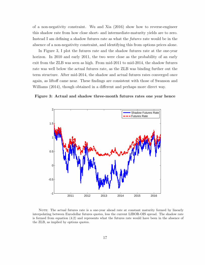
In Figure 3, I plot the futures rate and the shadow futures rate at the one-year
horizon. In 2010 and early 2011, the two were close as the probability of an early
exit from the ZLB was seen as high. From mid-2011 to mid-2014, the shadow futures
rate was well below the actual futures rate, as the ZLB was binding further out the
term structure. After mid-2014, the shadow and actual futures rates converged once
again, as liftoff came near. These findings are consistent with those of Swanson and
Williams (2014), though obtained in a different and perhaps more direct way.
Figure 3: Actual and shadow three-month futures rates one year hence
2011 2012 2013 2014 2015 2016-1
-0.5
0
0.5
1
1.5
2
Shadow Futures RateFutures Rate
Note: The actual futures rate is a one-year ahead rate at constant maturity formed by linearlyinterpolating between Eurodollar futures quotes, less the current LIBOR-OIS spread. The shadow rateis formed from equation (4.2) and represents what the futures rate would have been in the absence ofthe ZLB, as implied by options quotes.
17
4.3 Calibration of the BGM model
To illustrate the use of the BGM model (discussed in subsection 2.3), I took at-the-
money swaptions prices on May 31, 2016, from Bloomberg, at 1, 2, 3, 5, 7 and 10
year exercise dates and 1, 2, 3, 5, 7 and 10 year underlying swap maturities, and
calibrated the BGM model parameterized as in equations (2.9) and (2.10), so as to
minimize the sum of squared swaptions pricing errors. Payoffs were discounted using
the zero-coupon yield curve11 of Gurkaynak, Sack, and Wright (2007)12. The cal-
ibrated parameters (a, b, c, d and β in the notation of these equations) then give a
complete characterization of the risk-neutral evolution of future interest rates, which
allow questions to be answered that cannot be addressed by looking at a single ma-
turity point in isolation.
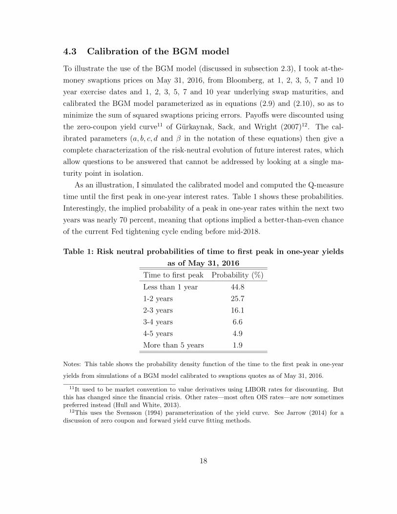
As an illustration, I simulated the calibrated model and computed the Q-measure
time until the first peak in one-year interest rates. Table 1 shows these probabilities.
Interestingly, the implied probability of a peak in one-year rates within the next two
years was nearly 70 percent, meaning that options implied a better-than-even chance
of the current Fed tightening cycle ending before mid-2018.
Table 1: Risk neutral probabilities of time to first peak in one-year yields
as of May 31, 2016
Time to first peak Probability (%)
Less than 1 year 44.8
1-2 years 25.7
2-3 years 16.1
3-4 years 6.6
4-5 years 4.9
More than 5 years 1.9
Notes: This table shows the probability density function of the time to the first peak in one-year
yields from simulations of a BGM model calibrated to swaptions quotes as of May 31, 2016.
11It used to be market convention to value derivatives using LIBOR rates for discounting. Butthis has changed since the financial crisis. Other rates—most often OIS rates—are now sometimespreferred instead (Hull and White, 2013).
12This uses the Svensson (1994) parameterization of the yield curve. See Jarrow (2014) for adiscussion of zero coupon and forward yield curve fitting methods.
18

4.4 Options implied pdfs and negative rates
In the US, the ZLB has consistently kept the federal funds rate above zero, and has
prevented three-month LIBOR from falling much below 50 basis points. Occasionally,
negative yields were observed in the secondary Treasury bill market, but these were
very isolated cases. The approach in the Black model, or in most papers in zero lower
bound literature (including Black (1995), Krippner (2014), Wu and Xia (2016) and
Kim and Singleton (2012)), is simply to rule out negative interest rates. This seems
appropriate in the US context. Federal Reserve Chair Janet Yellen stated in Congress
(February 11, 2016) that it was unclear if the FOMC had the legal authority to set
negative interest rates. That alone makes it quite unlikely that negative interest rates
will be used in the US.
But other countries grappling with overvalued currencies (especially Switzerland)
and/or sustained economic weakness (especially the euro area and Japan) have re-
sorted to negative interest rates. This has come as something of a surprise to many
observers. Nonetheless, to date, fears that this would lead to warehousing of large
amounts of cash have not proved correct (Rognlie, 2016), although there is surely
some tipping point that would lead the financial system to develop a new infras-
tructure to hold enormous cash balances. In these countries, the ZLB seems better
thought of a soft constraint. Options can then be used just as before to measure the
market assessment of how far rates might go into negative territory.
Euribor options are the euro-area analog of Eurodollar options. Although most of
the literature on options-implied interest rate densities is applied to the US, there have
been some applications to the euro area (Andersen and Wagener, 2002; Ivanova and
Gutierrez, 2014). Because of its size, and negative rates, the euro area is of special
significance at present. Consequently, Figure 4 plots the Q-measure pdf for euro-
area three-month interest rates in one year’s time, as of May 31, 2016. These were
obtained in the same way as for the US, again with an adjustment for the LIBOR-
OIS spread, though that was very modest. On May 31, 2016, the three-month euro
OIS rate was -34 basis points. The pdf implies low odds rates moving back above
zero, but substantial odds of rates moving somewhat further into negative territory
by mid-2017.
19

Figure 4: Risk Neutral PDF for euro-area three month rates one yearhence as of May 31, 2016
-1.5 -1 -0.5 0 0.50
0.5
1
1.5
Three Month OIS Rate (Percentage Points)
Note: This figure plots the (forward) risk neutral pdfs for three month OIS rates at the one-year-horizon for the euro area as of May 31, 2016. These are constructed by local linear regressions usingEuribor options, as described in the text. The density is shifted by the amount of the euro LIBOR-OISspread, so as to be interpretable as a pdf for three-month OIS rates.
4.5 Physical interest rate density forecasts
Generally time series models are used to construct P-measure interest rate forecasts.
However, in this paper, owing to the difficulties discussed in section 3 pertaining to
time series models of interest rates, especially in the current environment, I instead
use the Federal Reserve Bank of New York Primary Dealer survey. Figure 5 plots
the pdf for the target federal funds rate at the end of 2017 from the April 18, 2016
Primary Dealer survey13. The Q-measure pdf for the OIS rate over a three-month
13The survey asks respondents for the pdf conditional on moving to the ZLB at some point in 2016-2018, the pdf conditional on not moving to the ZLB at any point in 2016-2018, and the probabilityof moving to the ZLB during that period. Figure 5 plots the implied unconditional pdfs.
20

window centered around the end of 2017, as of the survey date, is also shown in the
figure. This was obtained from Eurodollar options, as discussed in subsection 4.1, and
represents an approximate Q-measure pdf for the target funds rate at the end of 2017.
This makes the P- and Q-measure pdfs as directly comparable as possible. Another
alternative would be to use Federal Funds futures options, which settle to the average
Figure 5: Physical (Survey) and Risk-Neutral PDFs for the end-2017funds rate as of April 18, 2016
0 0.5 1 1.5 2 2.5 3 3.50
5
10
15
20
25
30
35
40
Target Funds Rate
Per
cent
Pro
babi
lity
Note: This figure plots the survey probabilities for the target federal funds rate at the end of 2016from the Federal Reserve Bank of New York Primary Dealer Survey of April 18, 2016. Probabilities areput into bins that are 50 basis points wide, with the left-most bin referring to interest rates of less than50 basis points and the right-most bin referring to interest rates of greater than 3 percentage points. Thesurvey asks respondents for probabilities conditional on a return to the ZLB in 2016-2018, conditionalon no return to the ZLB in 2016-2018, and the probability of a return to the ZLB in that period. Theprobabilities plotted as bars in this figure are the implied unconditional probabilities. In addition, thefigure shows the corresponding risk neutral pdfs for three-month OIS rates on November 15, 2017 (at the18 month horizon—red dashed lines). These are constructed by local linear regressions using Eurodollaroptions, as described in the text. The density is shifted by the amount of the LIBOR-OIS spread, so asto be interpretable as a pdf for the federal funds rate around the end of 2017.
21

effective federal funds rate for a particular month. But these are very illiquid, except
at the shortest maturities.
A useful spinoff of the Primary Dealer survey is that it can be used to compute
the mean forecast of the federal funds rate, whereas most surveys are ambiguous as
to whether they elicit the mean, median or modal forecast (Engelberg, Manski, and
Williams, 2009). In Figure 5, the mean survey forecast for the funds rate at the end of
2017 was 1.38 percent whereas the corresponding modal forecast was 1.5 to 2 percent.
4.6 Pricing Kernel
In Figure 5, it can be seen that the survey reported 14% odds of the federal funds rate
being less than 50 basis points, with the rest of the probability mass being distinctly
away from the ZLB. Meanwhile, the Q-measure pdf derived from Eurodollar options
put much more mass on very low interest rates. The empirical pricing kernel—the
ratio of Q- to P-measure pdfs—is thus downward sloping. Figure 6 plots the pricing
kernel constructed in this way on April 18, 2016, and also on dates in April 2014 and
April 2015, likewise constructed from the Primary Dealer survey for interest rates at
the end of the following year, coupled with Eurodollar options quotes.
Most researchers have found pricing kernels to be U-shaped in interest rates. Li
and Zhao (2009) computed the pricing kernel by comparing P- and Q-measure pdfs
using interest rate caps from 2000 to 2004. They found that it was U-shaped in
interest rates—both very high and very low interest rates were high marginal utility
states of the world. Ivanova and Gutierrez (2014) also found U-shaped pricing kernels
using Euribor options data from 2006 to 2012. In Figure 6, I also find something
of a U-shaped pattern in the empirical pricing kernel in 2014 and 2015. But in
2016, I find that investors are willing to pay a premium to hedge against the low
interest rate states of the world, but not the high interest rate states. This may be
reasonable, as the predominant macroeconomic worry today is slow growth, deflation
and/or financial instability—circumstances that will be associated with low levels of
the federal funds rate (Campbell, Sunderam, and Viceira, 2009). It is also entirely
consistent with the finding that term premia are presently negative in the models
of Kim and Wright (2005) and Adrian, Crump, and Moench (2013), although those
papers focus on the Treasury term premium, not the term premium in short-term
22

money market futures14. The differences between my results and those of Li and
Zhao and Ivanova and Gutierez arise because I use more recent data and take the
P-measure pdf from surveys, not from time series methods. Ivanova and Gutierez use
six-year rolling windows of actual interest rates to form the P-measure pdf, and while
that might be reasonable in normal times, I prefer to use survey evidence given the
unusual recent behavior of interest rates.
Figure 6: Empirical Pricing Kernels
0 0.5 1 1.5 2 2.5 3 3.50
0.5
1
1.5
2
2.5
3
3.5
4
4.5
5
Target Funds Rate
Pric
ing
Ker
nel
201420152016
Note: This figure plots the empirical pricing kernel constructed as the ratio of the risk-neutral pdfsfor three-month OIS rates at the 18 month horizon to the survey probabilities for the target federalfunds rate at the end of the following year from the Federal Reserve Bank of New York Primary DealerSurveys of April 22, 2014, April 20, 2015 and April 18, 2016. Survey probabilities are put into bins thatare 50 basis points wide. Risk-neutral pdfs are constructed by local linear regressions using Eurodollaroptions, as described in the text. The density is shifted by the amount of the LIBOR-OIS spread, so asto be interpretable as a pdf for the federal funds rate around the end of following year.
14At the time of writing, the term premium in short-term interest rate futures has to be negativein order to give a reasonable expected path of monetary policy.
23

5 Conclusion
With the wealth of interest rate derivatives that trade in deep and liquid markets,
researchers can identify the state price density for future interest rates with great pre-
cision and minimal assumptions. The physical density is much harder to recover, but
progress can be made on that front too, via time series econometric methods and/or
surveys. Depending on the purpose, researchers may be most interested in either the
physical or risk-neutral density (Feldman, Heinecke, Kocherlakota, Schulhofer-Wohl,
and Tallarini, 2015)
In this paper, I have reviewed methods for interest rate density forecasting under
both risk-neutral and physical measures. I have shown some illustrative applications,
with particular focus on issues relating to the zero lower bound. The main goal of these
applications is to show that forward looking estimates of interest rate distributions are
important not just to finance practitioners, but also in macroeconomics and monetary
economics, where these methods remain regrettably underutilized.
References
Adrian, T., R. K. Crump, and E. Moench (2013): “Pricing the term structure
with linear regressions,” Journal of Financial Economics, 110, 110–138.
Aıt-Sahalia, Y., and J. Duarte (2003): “Nonparametric option pricing under
shape restrictions,” Journal of Econometrics, 116, 9–47.
Aıt-Sahalia, Y., and A. W. Lo (1998): “Nonparameteric estimation of state-price
densities implicit in financial asset prices,” Journal of Finance, 53, 499–547.
Andersen, A. B., and T. Wagener (2002): “Extracting risk neutral probability
densities by fitting implied volatility smiles: some methodological points and an
application to the 3M Euribor futures option prices,” ECB Working Paper 198.
Andersen, T., and L. Benzoni (2010): “Do bonds span volatility risk in the U.S.
Treasury market? A specification test for affine term structure models,” Journal
of Finance, 65, 603–653.
24

Black, F. (1976): “The pricing of commodity contracts,” Journal of Financial
Economics, 3, 167–179.
(1995): “Interest rates as options,” Journal of Finance, 50, 1371–1376.
Bliss, R. R., and N. Panigirtzoglou (2002): “Testing the Stability of Implied
Probability Density Functions,” Journal of Banking and Finance, 26, 381–422.
Brace, A., D. Gatarek, and M. Musiela (1997): “The market model of interest
rate dynamics,” Mathematical Finance, 7, 127–154.
Breeden, D. T., and R. H. Litzenberger (1978): “Prices of state contingent
claims implicit in options prices,” Journal of Business, 51, 621–651.
Brigo, D., and F. Mercurio (2006): Interest rate models—Theory and practice.
Springer.
Campbell, J. Y., A. Sunderam, and L. M. Viceira (2009): “Inflation Bets or
Deflation Hedges? The Changing Risks of Nominal Bonds,” NBER Working Paper
14701.
Carriero, A., T. E. Clark, and M. G. Marcellino (2014): “No arbitrage pri-
ors, drifting volatilities and the term structure of interest rates,” CEPR Discussion
Paper 9848.
Chun, A. L. (2011): “Expectations, bond yields, and monetary policy,” Review of
Financial Studies, 24, 208–247.
Cieslak, A., and P. Povala (2016): “Information in the term structure of yield
curve volatility,” Journal of Finance, 71, 1393–1436.
Clark, T. E. (2011): “Real-time density forecasts from bayesian vector autoregres-
sions with stochastic volatility,” Journal of Business and Economic Statistics, 29,
327–341.
Cochrane, J. H., and M. Piazzesi (2005): “Bond risk premia,” American Eco-
nomic Review, 95, 138–160.
25

Collin-Dufresne, P., and R. S. Goldstein (2002): “Do bonds span the fixed
income markets? Theory and evidence for unspanned stochastic volatility,” Journal
of Finance, 57, 1685–1730.
Collin-Dufresne, P., R. S. Goldstein, and C. S. Jones (2009): “Can interest
rate volatility be extracted from the cross section of bond yields?,” Journal of
Financial Economics, 94, 47–66.
Diebold, F. X., and C. Li (2006): “Forecasting the term structure of government
bond yields,” Journal of Econometrics, 131, 309–338.
Duffee, G. R. (2013): “Forecasting interest rates,” in Handbook of Economic Fore-
casting, Volume 2, ed. by G. Elliott, and A. Timmermann. Elsevier.
Egorov, Alexei, V., Y. Hong, and H. Li (2006): “Validating forecasts of the
joint probability density of bond yields: Can affine models beat random walk?,”
Journal of Econometrics, 135, 255–284.
Elliott, D., and J. Noss (2015): “Estimating market expectations of changes in
bank rate,” Bank of England Quarterly Bulletin, 55, 273–282.
Engelberg, J., C. F. Manski, and J. Williams (2009): “Comparing the point
predictions and subjective probability distributions of professional forecasters,”
Journal of Business and Economic Statistics, 27, 30–41.
Feldman, R., K. Heinecke, N. Kocherlakota, S. Schulhofer-Wohl, and
T. Tallarini (2015): “Market-Based Probabilities: A Tool for Policymakers,”
Federal Reserve Bank of Minneapolis Working Paper.
Filipovic, D., M. Larsson, and A. B. Trolle (forthcoming): “Linear-rational
term structure models,” Journal of Finance.
Goldys, B., M. Musiela, and D. Sondermann (2000): “Lognormality of rates
and term structure models,” Stochastic analysis and applications, 18, 375–396.
Gurkaynak, R. S., B. Sack, and J. H. Wright (2007): “The U.S. Treasury
yield curve: 1961 to the present,” Journal of Monetary Economics, 54, 2291–2304.
26
Hautsch, N., and Y. Ou (2012): “Analyzing interest rate risk: Stochastic volatility
in the term structure of government bond yields,” Journal of Banking and Finance,
36, 2988–3007.
Hautsch, N., and F. Yang (2012): “Bayesian Inference in a Stochastic Volatility
Nelson-Siegel Model,” Computational Statistics and Data Analysis, 56, 3774–3792.
Heath, D., R. A. Jarrow, and A. Morton (1992): “Bond pricing and the term
structure of interest rates: a new methodology for contingent claims valuation,”
Econometrica, 60, 77–105.
Heidari, M., and L. Wu (2009): “A joint framework for consistently pricing interest
rates and interest rate derivatives,” Journal of Financial and Quantiative Analysis,
44, 517–550.
Hong, Y., H. Li, and F. Zhao (2004): “Out-of-Sample Performance of Discrete
Time Spot Interest Rate Models,” Journal of Business and Economic Statistics,
22, 457–473.
Hull, J., and A. White (1990): “Pricing interest-rate derivative securities,” Review
of Financial Studies, 3, 573–592.
(2013): “LIBOR vs. OIS: The derivatives discount dilemma,” Journal of
Investment Management, 11:3, 14–27.
Ivanova, V., and J. M. Gutierrez (2014): “Interest rate forecasts, state price
densities and risk premium from Euribor options,” .
Jacobs, K., and L. Karoui (2009): “Conditional volatility in affine term-structure
models: Evidence from Treasury and swap markets,” Journal of Financial Eco-
nomics, 91, 288–318.
Jamshidian, F. (2007): “An exact bond option formula,” Journal of Finance, 44,
205–209.
Jarrow, R. A. (2009): “The term structure of interest rates,” Annual Review of
Financial Economics, 1, 69–96.
(2014): “Forward rate curve smoothing,” Annual Review of Financial Eco-
nomics, 6, 443–458.
27
Jarrow, R. A., H. Li, and F. Zhao (2007): “Interest rate caps ‘smile’ too! But
can the LIBOR market models capture the smile?,” Journal of Finance, 62, 345–
382.
Kim, D. H., and A. Orphanides (2012): “Term Structure Estimation with Survey
Data on Interest Rate Forecasts,” Journal of Financial and Quantitative Analysis,
47, 241–272.
Kim, D. H., and K. J. Singleton (2012): “Term structure models and the zero
bound: An empirical investigation of Japanese yields,” Journal of Econometrics,
170, 32–49.
Kim, D. H., and J. H. Wright (2005): “An arbitrage-free three-factor term struc-
ture model and the recent behavior of long-term yields and distant-horizon forward
rates,” Finance and Economics Discussion Series, 2005-33.
(2014): “Jumps in Bond Yields at Known Times,” Finance and Economics
Discussion Series, 2014-100.
Koopman, S. J., M. I. P. Mallee, and M. V. der Wel (2010): “Analyzing the
term structure of interest rates using the dynamic Nelson-Siegel model with time-
varying parameters,” Journal of Business and Economic Statistics, pp. 329–343.
Krippner, L. (2014): Zero lower bound term structure modeling: A practitioner’s
guide. Palgrave Macmillan.
Li, H., and F. Zhao (2009): “Nonparametric estimation of state-price densities
implicit in interest rate cap prices,” Review of Financial Studies, 22, 4335–4376.
Litterman, R., and J. Scheinkman (1991): “Common factors affecting bond
returns,” Journal of Fixed Income, 1, 54–61.
Longstaff, F. A., and E. S. Schwartz (1992): “Interest rate volatility and the
term structure: A two-factor general equilibrium model,” Journal of Finance, 48,
1259–1282.
Nelson, C. R., and A. F. Siegel (1987): “Parsimonious modeling of yield curves,”
Journal of Business, 60, 473–489.
28

Rebonato, R. (1999): Volatility and Correlation. Wiley.
(2003): Modern pricing of interest rate derivatives: The LIBOR market
model and beyond. Princeton University Press.
Rognlie, M. (2016): “What lower bound? Monetary policy with negative interest
rates,” Working Paper, MIT.
Rosenberg, J. V., and R. F. Engle (2002): “Empirical pricing kernels,” Journal
of Financial Economics, 64, 341–372.
Sandmann, K., and D. Sondermann (1997): “A note on the stability of lognormal
interest rate models and the pricing of eurodollar futures,” Mathematical Finance,
7, 119–125.
Shiller, R. J., J. Y. Campbell, and K. L. Schoenholtz (1983): “Forward
rates and future policy: Interpreting the term structure of interest rates,” Brookings
Papers on Economic Activity, 1, 173–217.
Shimko, D. (1993): “Bounds of Probability,” Risk, 6, 33–37.
Shreve, S. E. (2004): Stochastic calculus for finance II: Continuous-time models.
Springer.
Svensson, L. E. O. (1994): “Estimating and interpreting forward rates: Sweden
1992-4,” National Bureau of Economic Research Working Paper 4871.
Swanson, E. T., and J. C. Williams (2014): “Measuring the effect of the zero
lower bound on medium- and longer-term interest rates,” American Economic Re-
view, 104, 3154–3185.
Veronesi, P. (2010): Fixed income securities. Wiley.
Wright, J. H. (forthcoming): “Options-implied probability density functions for
real interest rates,” International Journal of Central Banking.
Wu, J. C., and F. D. Xia (2016): “Measuring the Macroeconomic Impact of
Monetary Policy at the Zero Lower Bound,” Journal of Money, Credit and Banking,
48, 253–291.
29