Embed Size (px)
Citation preview

Fortranfor Environmental Science
Brian Hanson
University of Delaware
c©2014

FortranTable of ContentsI. Basic Elements of Fortran . . . . . . . . . . . . . . . . . . . . . . . . . . . . . 11. Fortran History . . . . . . . . . . . . . . . . . . . . . . . . . . . . . . . . . . 2
Standards . . . . . . . . . . . . . . . . . . . . . . . . . . . . . . . . . . . 5Chronology . . . . . . . . . . . . . . . . . . . . . . . . . . . . . . . . . . 6
2. Statements and Source Code . . . . . . . . . . . . . . . . . . . . . . . . . . . . 7Code and other files . . . . . . . . . . . . . . . . . . . . . . . . . . . . . . . 7Statements . . . . . . . . . . . . . . . . . . . . . . . . . . . . . . . . . . . 8Names and Keywords . . . . . . . . . . . . . . . . . . . . . . . . . . . . . . 9Character Set . . . . . . . . . . . . . . . . . . . . . . . . . . . . . . . . . 9Statement Classification . . . . . . . . . . . . . . . . . . . . . . . . . . . . . 9A Simple Program . . . . . . . . . . . . . . . . . . . . . . . . . . . . . . 10
3. Data Types . . . . . . . . . . . . . . . . . . . . . . . . . . . . . . . . . . 13REAL . . . . . . . . . . . . . . . . . . . . . . 13Literal representation of REAL: . . . . . . . . . . . . . . . . . . . . . . 14Declaring Real Variables: . . . . . . . . . . . . . . . . . . . . . . . . . 14INTEGER . . . . . . . . . . . . . . . . . . . . . . . . . . . . . . . . 14Literal Representation of Integers: . . . . . . . . . . . . . . . . . . . . . . 15Declaration of Integers: . . . . . . . . . . . . . . . . . . . . . . . . . . 15CHARACTER . . . . . . . . . . . . . . . . . . . . . . . . . . . . . . 15Literal Representation of Character Strings: . . . . . . . . . . . . . . . . . 15Declaration of Character strings: . . . . . . . . . . . . . . . . . . . . . . 15
4. Arithmetic . . . . . . . . . . . . . . . . . . . . . . . . . . . . . . . . . . . 16Replacement or Assignment Statement . . . . . . . . . . . . . . . . . . . . . 16
Numeric Operators . . . . . . . . . . . . . . . . . . . . . . . . . . . . 16Integer and Mixed-Mode Arithmetic . . . . . . . . . . . . . . . . . . . . . . 16Intrinsic Functions . . . . . . . . . . . . . . . . . . . . . . . . . . . . . . 17Order of Precedence . . . . . . . . . . . . . . . . . . . . . . . . . . . . . 18A few equation examples . . . . . . . . . . . . . . . . . . . . . . . . . . . 19
5. Input/Output . . . . . . . . . . . . . . . . . . . . . . . . . . . . . . . . . 20I/O Statements . . . . . . . . . . . . . . . . . . . . . . . . . . . . . . . . 20
READ . . . . . . . . . . . . . . . . . . . . . . . . . . . . . . . . . . 20WRITE . . . . . . . . . . . . . . . . . . . . . . . . . . . . . . . . . 20OPEN . . . . . . . . . . . . . . . . . . . . . . . . . . . . . . . . . . 20
Format Information . . . . . . . . . . . . . . . . . . . . . . . . . . . . . . 21Edit Descriptors . . . . . . . . . . . . . . . . . . . . . . . . . . . . . . . 21
Data edit descriptors . . . . . . . . . . . . . . . . . . . . . . . . . . . 21Control edit descriptors . . . . . . . . . . . . . . . . . . . . . . . . . . 22Character string edit descriptors: . . . . . . . . . . . . . . . . . . . . . . 22
Unit Numbers and File Information . . . . . . . . . . . . . . . . . . . . . . . 236. Control Structures . . . . . . . . . . . . . . . . . . . . . . . . . . . . . . . 24
Counted DO loop . . . . . . . . . . . . . . . . . . . . . . . . . . . . . . . 24IF blocks . . . . . . . . . . . . . . . . . . . . . . . . . . . . . . . . . . 25
Single-statement IF . . . . . . . . . . . . . . . . . . . . . . . . . . . . 26Logical expressions . . . . . . . . . . . . . . . . . . . . . . . . . . . . . . 26
Logical operators. . . . . . . . . . . . . . . . . . . . . . . . . . . . . . 27Unlimited DO loop . . . . . . . . . . . . . . . . . . . . . . . . . . . . . . 27EXIT and CYCLE . . . . . . . . . . . . . . . . . . . . . . . . . . . . . . 28Direct Transfers . . . . . . . . . . . . . . . . . . . . . . . . . . . . . . . 28
GO TO statement . . . . . . . . . . . . . . . . . . . . . . . . . . . . 28STOP statement . . . . . . . . . . . . . . . . . . . . . . . . . . . . . 28
7. Arrays . . . . . . . . . . . . . . . . . . . . . . . . . . . . . . . . . . . . 29Initialization, Literal Representation . . . . . . . . . . . . . . . . . . . . . . . 29Array References, Array Sections . . . . . . . . . . . . . . . . . . . . . . . . 30Array Arithmetic . . . . . . . . . . . . . . . . . . . . . . . . . . . . . . . 30Intrinsic Functions used with Arrays . . . . . . . . . . . . . . . . . . . . . . 30
Elemental Functions. . . . . . . . . . . . . . . . . . . . . . . . . . . . 30Functions that Operate Only on Arrays. . . . . . . . . . . . . . . . . . . . 31
Array Example . . . . . . . . . . . . . . . . . . . . . . . . . . . . . . . . 32
ii
Contents iii
8. Module Subroutines . . . . . . . . . . . . . . . . . . . . . . . . . . . . . . . 33Subroutines and Modules . . . . . . . . . . . . . . . . . . . . . . . . . . . 33
INTENT attributes. . . . . . . . . . . . . . . . . . . . . . . . . . . . . 34Assumed-Shape arrays. . . . . . . . . . . . . . . . . . . . . . . . . . . 35Local Variables and SAVE. . . . . . . . . . . . . . . . . . . . . . . . . . 35
Calling a Subroutine . . . . . . . . . . . . . . . . . . . . . . . . . . . . . 36USE . . . . . . . . . . . . . . . . . . . . . . . . . . . . . . . . . . . 36CALL . . . . . . . . . . . . . . . . . . . . . . . . . . . . . . . . . . 36RETURN . . . . . . . . . . . . . . . . . . . . . . . . . . . . . . . . 37
A Module Subroutine Example . . . . . . . . . . . . . . . . . . . . . . . . . 37Argument Association . . . . . . . . . . . . . . . . . . . . . . . . . . . . . 38
II. Advanced Fortran . . . . . . . . . . . . . . . . . . . . . . . . . . . . . . . 409. Data Types . . . . . . . . . . . . . . . . . . . . . . . . . . . . . . . . . . 41
Numeric Types. . . . . . . . . . . . . . . . . . . . . . . . . . . . . . . . . 42INTEGER. . . . . . . . . . . . . . . . . . . . . . . . . . . . . . . . . 42Declaration of Integers. . . . . . . . . . . . . . . . . . . . . . . . . . . 42Literal Representation of Integers: . . . . . . . . . . . . . . . . . . . . . . 43BOZ constants . . . . . . . . . . . . . . . . . . . . . . . . . . . . . . 43REAL. . . . . . . . . . . . . . . . . . . . . . . . . . . . . . . . . . 43Literal representation of Real: . . . . . . . . . . . . . . . . . . . . . . . 44Declaring Real Variables: . . . . . . . . . . . . . . . . . . . . . . . . . 45Precision and KIND. . . . . . . . . . . . . . . . . . . . . . . . . . . . . 45COMPLEX. . . . . . . . . . . . . . . . . . . . . . . . . . . . . . . . 46Declaration of complex numbers. . . . . . . . . . . . . . . . . . . . . . . 46Literal representation of complex numbers: . . . . . . . . . . . . . . . . . . 46Complex arithmetic: . . . . . . . . . . . . . . . . . . . . . . . . . . . . 46
NonNumeric Types. . . . . . . . . . . . . . . . . . . . . . . . . . . . . . . 47CHARACTER . . . . . . . . . . . . . . . . . . . . . . . . . . . . . . 47Literal Representation of Character Strings: . . . . . . . . . . . . . . . . . 47Declaration of Character strings: . . . . . . . . . . . . . . . . . . . . . . 47Collating sequence. . . . . . . . . . . . . . . . . . . . . . . . . . . . . 48LOGICAL. . . . . . . . . . . . . . . . . . . . . . . . . . . . . . . . . 48Literal Representation of Logical . . . . . . . . . . . . . . . . . . . . . . 48Declaration of Logical: . . . . . . . . . . . . . . . . . . . . . . . . . . . 48Logical Arithmetic: . . . . . . . . . . . . . . . . . . . . . . . . . . . . 49Order of Precedence with Logical Operators. . . . . . . . . . . . . . . . . . 51
10. Input/Output . . . . . . . . . . . . . . . . . . . . . . . . . . . . . . . . . 52READ statements . . . . . . . . . . . . . . . . . . . . . . . . . . . . . . . 52
IOSTAT and END options. . . . . . . . . . . . . . . . . . . . . . . . . . 53More options for READ statements. . . . . . . . . . . . . . . . . . . . . . 53
WRITE . . . . . . . . . . . . . . . . . . . . . . . . . . . . . . . . . . . 54More options for WRITE statements. . . . . . . . . . . . . . . . . . . . . 54
OPEN . . . . . . . . . . . . . . . . . . . . . . . . . . . . . . . . . . . . 54More options for OPEN statements. . . . . . . . . . . . . . . . . . . . . . 55A direct access example. . . . . . . . . . . . . . . . . . . . . . . . . . . 57Preconnected unit numbers. . . . . . . . . . . . . . . . . . . . . . . . . 57
Formats . . . . . . . . . . . . . . . . . . . . . . . . . . . . . . . . . . . 58Edit Descriptors . . . . . . . . . . . . . . . . . . . . . . . . . . . . . 58Data edit descriptors . . . . . . . . . . . . . . . . . . . . . . . . . . . 58Data edit descriptor modifiers. . . . . . . . . . . . . . . . . . . . . . . . 60Control edit descriptors . . . . . . . . . . . . . . . . . . . . . . . . . . 61Character string edit descriptors: . . . . . . . . . . . . . . . . . . . . . . 62
NAMELIST . . . . . . . . . . . . . . . . . . . . . . . . . . . . . . . . . 62INQUIRE . . . . . . . . . . . . . . . . . . . . . . . . . . . . . . . . . . 63Other I/O statements . . . . . . . . . . . . . . . . . . . . . . . . . . . . . 64
CLOSE . . . . . . . . . . . . . . . . . . . . . . . . . . . . . . . . . 65
REWIND . . . . . . . . . . . . . . . . . . . . . . . . . . . . . . . . 65BACKSPACE . . . . . . . . . . . . . . . . . . . . . . . . . . . . . . 65ENDFILE . . . . . . . . . . . . . . . . . . . . . . . . . . . . . . . . 65
Stream and Asynchronous . . . . . . . . . . . . . . . . . . . . . . . . . . . 65Stream I/O . . . . . . . . . . . . . . . . . . . . . . . . . . . . . . . 65Asynchronous I/O and buffering . . . . . . . . . . . . . . . . . . . . . . 65
11. Control Structures . . . . . . . . . . . . . . . . . . . . . . . . . . . . . . . 66

iv Contents
Basic Control Constructs . . . . . . . . . . . . . . . . . . . . . . . . . . . 66IF constructs . . . . . . . . . . . . . . . . . . . . . . . . . . . . . . 66DO loops. . . . . . . . . . . . . . . . . . . . . . . . . . . . . . . . . 66Counted DO loop . . . . . . . . . . . . . . . . . . . . . . . . . . . . . 66Uncontrolled DO loops . . . . . . . . . . . . . . . . . . . . . . . . . . 67DO WHILE loop. . . . . . . . . . . . . . . . . . . . . . . . . . . . . . 69Modifying Loops, and Loop Labels. . . . . . . . . . . . . . . . . . . . . . 69
CASE structures . . . . . . . . . . . . . . . . . . . . . . . . . . . . . . . 71Other Control Constructs . . . . . . . . . . . . . . . . . . . . . . . . . . . 72
12. Arrays . . . . . . . . . . . . . . . . . . . . . . . . . . . . . . . . . . . . 73Size, Shape, Rank, and Bounds . . . . . . . . . . . . . . . . . . . . . . . . . 74
Storage Sequence. . . . . . . . . . . . . . . . . . . . . . . . . . . . . . . . 74Array Constructors . . . . . . . . . . . . . . . . . . . . . . . . . . . . . . 75
Array Triple. . . . . . . . . . . . . . . . . . . . . . . . . . . . . . . . 76Array Arithmetic . . . . . . . . . . . . . . . . . . . . . . . . . . . . . . . 76Intrinsic Functions with Arrays . . . . . . . . . . . . . . . . . . . . . . . . . 77
DIM arguments. . . . . . . . . . . . . . . . . . . . . . . . . . . . . . 77MASK arguments. . . . . . . . . . . . . . . . . . . . . . . . . . . . . 78
Allocatable Arrays . . . . . . . . . . . . . . . . . . . . . . . . . . . . . . 78Array Assignment with WHERE . . . . . . . . . . . . . . . . . . . . . . . . 79FORALL array assignment . . . . . . . . . . . . . . . . . . . . . . . . . . . 80
13. Scoping Units . . . . . . . . . . . . . . . . . . . . . . . . . . . . . . . . . 81Programs . . . . . . . . . . . . . . . . . . . . . . . . . . . . . . . . . . 81Modules . . . . . . . . . . . . . . . . . . . . . . . . . . . . . . . . . . . 81
PUBLIC, PRIVATE. . . . . . . . . . . . . . . . . . . . . . . . . . . . 81Subroutines and Functions . . . . . . . . . . . . . . . . . . . . . . . . . . . 82
SUBROUTINE. . . . . . . . . . . . . . . . . . . . . . . . . . . . . . 82FUNCTION. . . . . . . . . . . . . . . . . . . . . . . . . . . . . . . . 82
Declaration Attributes within Subroutines and Functions . . . . . . . . . . . . . 82INTENT(IN), INTENT(OUT), INTENT(INOUT). . . . . . . . . . . . . . . 82Assumed-shape arrays. . . . . . . . . . . . . . . . . . . . . . . . . . . 83
Related Statements . . . . . . . . . . . . . . . . . . . . . . . . . . . . . . 83CALL. . . . . . . . . . . . . . . . . . . . . . . . . . . . . . . . . . . 83CONTAINS. . . . . . . . . . . . . . . . . . . . . . . . . . . . . . . . 83USE. . . . . . . . . . . . . . . . . . . . . . . . . . . . . . . . . . . 83RETURN. . . . . . . . . . . . . . . . . . . . . . . . . . . . . . . . . 84
A Module Subroutine Example . . . . . . . . . . . . . . . . . . . . . . . . . 84Argument Association . . . . . . . . . . . . . . . . . . . . . . . . . . . . . 86A User-Defined Function Example . . . . . . . . . . . . . . . . . . . . . . . 87Internal Procedures . . . . . . . . . . . . . . . . . . . . . . . . . . . . . . 88External Procedures and Interfaces . . . . . . . . . . . . . . . . . . . . . . . 89
14. Derived Types and Pointers . . . . . . . . . . . . . . . . . . . . . . . . . . . 90Defining a Derived Type . . . . . . . . . . . . . . . . . . . . . . . . . . . . 90Extending a Derived Type . . . . . . . . . . . . . . . . . . . . . . . . . . . 92Pointers . . . . . . . . . . . . . . . . . . . . . . . . . . . . . . . . . . . 93
Appendices . . . . . . . . . . . . . . . . . . . . . . . . . . . . . . . . . . . 94Appendix A. Fortran Intrinsic Procedures . . . . . . . . . . . . . . . . . . . . . . 95
Number models. . . . . . . . . . . . . . . . . . . . . . . . . . . . . . 95The Intrinsic Procedures . . . . . . . . . . . . . . . . . . . . . . . . . . 96
Appendix B. ASCII Codes . . . . . . . . . . . . . . . . . . . . . . . . . . . . . 119Appendix C. Fortran Archeology . . . . . . . . . . . . . . . . . . . . . . . . . . 121
Language Evolution . . . . . . . . . . . . . . . . . . . . . . . . . . . . . . 121Old Fortran . . . . . . . . . . . . . . . . . . . . . . . . . . . . . . . . . 123Fixed Form Source . . . . . . . . . . . . . . . . . . . . . . . . . . . . . . 123What Old Fortran never had: . . . . . . . . . . . . . . . . . . . . . . . . . . 124
No Array Arithmetic or Array Section references. . . . . . . . . . . . . . . . 124
No Elemental Functions. . . . . . . . . . . . . . . . . . . . . . . . . . . 124No Array Reduction and Manipulation Functions. . . . . . . . . . . . . . . . 124No Attributes with Declarations. . . . . . . . . . . . . . . . . . . . . . . 124Simpler END statements . . . . . . . . . . . . . . . . . . . . . . . . . . 124No MODULEs. . . . . . . . . . . . . . . . . . . . . . . . . . . . . . . 124No SUBROUTINE interfaces, . . . . . . . . . . . . . . . . . . . . . . . 124Missing Control Structures. . . . . . . . . . . . . . . . . . . . . . . . . 124

Contents v
KIND parameters were less standard. . . . . . . . . . . . . . . . . . . . . 124Many fewer intrinsic functions. . . . . . . . . . . . . . . . . . . . . . . . 125Old logical operators. . . . . . . . . . . . . . . . . . . . . . . . . . . . 125No dynamic allocation. . . . . . . . . . . . . . . . . . . . . . . . . . . 125Other advanced features. . . . . . . . . . . . . . . . . . . . . . . . . . . 125Basic Linear Algebra Subprograms. . . . . . . . . . . . . . . . . . . . . . 125
Things that were about the same. . . . . . . . . . . . . . . . . . . . . . . . . 125Intrinsic Types. . . . . . . . . . . . . . . . . . . . . . . . . . . . . . . 125Control structures: . . . . . . . . . . . . . . . . . . . . . . . . . . . . 125IMPLICIT NONE . . . . . . . . . . . . . . . . . . . . . . . . . . . 125Arithmetic . . . . . . . . . . . . . . . . . . . . . . . . . . . . . . . . 125
Input/Output and FORMAT . . . . . . . . . . . . . . . . . . . . . . . . 125Commonly used, useful things that have been replaced: . . . . . . . . . . . . . . 126
COMMON blocks. . . . . . . . . . . . . . . . . . . . . . . . . . . . . . 126DATA statements. . . . . . . . . . . . . . . . . . . . . . . . . . . . . 126
Standard Fortran 77 . . . . . . . . . . . . . . . . . . . . . . . . . . . . . . 126No END DO. . . . . . . . . . . . . . . . . . . . . . . . . . . . . . . 126No DO WHILE. . . . . . . . . . . . . . . . . . . . . . . . . . . . . . 126No IMPLICIT NONE. . . . . . . . . . . . . . . . . . . . . . . . . . 126No Mixed Case. . . . . . . . . . . . . . . . . . . . . . . . . . . . . . . 126Symbolic names limited to 6 characters. . . . . . . . . . . . . . . . . . . . 126No embedded comments. . . . . . . . . . . . . . . . . . . . . . . . . . . 127
Standard Fortran 66 . . . . . . . . . . . . . . . . . . . . . . . . . . . . . . 127No Block IF. . . . . . . . . . . . . . . . . . . . . . . . . . . . . . . 127No CHARACTER data type. . . . . . . . . . . . . . . . . . . . . . . . 127No Standard and Generic Functions. . . . . . . . . . . . . . . . . . . . . 127No OPEN. . . . . . . . . . . . . . . . . . . . . . . . . . . . . . . . . 128
Confronting Old Codes . . . . . . . . . . . . . . . . . . . . . . . . . . . . 128Old Features from Old Fortran . . . . . . . . . . . . . . . . . . . . . . . . . 129Deleted Features . . . . . . . . . . . . . . . . . . . . . . . . . . . . . . . 129
Hollerith Data and nH edit descriptor. . . . . . . . . . . . . . . . . . . . 129NonInteger Do Index Variables . . . . . . . . . . . . . . . . . . . . . . . 130Branching to an END IF from outside the IF block. . . . . . . . . . . . . 131PAUSE statement. . . . . . . . . . . . . . . . . . . . . . . . . . . . . 131ASSIGN statement, assigned GO TO and assigned FORMAT. . . . . . . . . 131
Obsolescent Features . . . . . . . . . . . . . . . . . . . . . . . . . . . . . 132Computed GOTO. . . . . . . . . . . . . . . . . . . . . . . . . . . . . 132Arithmetic IF. . . . . . . . . . . . . . . . . . . . . . . . . . . . . . . 132Old-Style DO terminations. . . . . . . . . . . . . . . . . . . . . . . . . 133Alternate RETURN. . . . . . . . . . . . . . . . . . . . . . . . . . . . 134Fixed-Form Source. . . . . . . . . . . . . . . . . . . . . . . . . . . . . 134Data statements in executable. . . . . . . . . . . . . . . . . . . . . . . . 134Statement Functions. . . . . . . . . . . . . . . . . . . . . . . . . . . . 134CHARACTER*n declarations. . . . . . . . . . . . . . . . . . . . . . . . 134Assumed-Length Character Functions. . . . . . . . . . . . . . . . . . . . . 134
Deprecated Features . . . . . . . . . . . . . . . . . . . . . . . . . . . . . . 135COMMON blocks. . . . . . . . . . . . . . . . . . . . . . . . . . . . . . 135BLOCK DATA subprograms. . . . . . . . . . . . . . . . . . . . . . . . 136EQUIVALENCE statements. . . . . . . . . . . . . . . . . . . . . . . . 136Call-by-Address tricks with external subroutines. . . . . . . . . . . . . . . . 136Alternate ENTRY. . . . . . . . . . . . . . . . . . . . . . . . . . . . . 140Implicit typing and IMPLICIT statements. . . . . . . . . . . . . . . . . 140Missing “Prettyprinting”, short variable names. . . . . . . . . . . . . . . . . 141Carriage Control. . . . . . . . . . . . . . . . . . . . . . . . . . . . . . 142External Procedures. . . . . . . . . . . . . . . . . . . . . . . . . . . . 142
Fonts and typography are used to help indicate context.
• Italics are used for emphasis and boldface is used to indicate concepts that
need definitions.
• Literal Fortran code is in a typewriter face, in which Fortran-defined keywords
are uppercase, such as READ or PROGRAM, a user’s made-up variable names are
lowercase typewriter face, module, subroutine, or program names are Ti-
tle Capitalized, and Fortran’s built-in intrinsic functions and subroutines
will be slightly slanted, like MAX and COS.
• Concept names that need to be replaced in Fortran code are in this font. E.g.,
in READ (1,*) input list, everything up to the right parenthesis could be typed
literally into the computer, but input listmust be replaced with a list of variables
to be read.
• Comments that need to be embedded in Fortran code may look like this.
• In cases where a blank space character must be “visible” to be counted, it will
be denoted by a symbol. Obvious single blanks separating syntactic items
are not marked this way.
Fortran version. This writeup primarily deals with Fortran as of the Fortran 95
standard (see the History section for a discussion of the time-varying standards).
A few items that from the Fortran 2003 standard are included, particularly if those
things have been widely implemented in available compilers. This text tries to
be forward compatible, meaning that code written to conform to the Fortran 95
standard will still work the same way when complete Fortran 2003 or Fortran 2008
compilers are available.
vi

I. Basic Elements of FortranIn your native language, you know some thousands of words that you use in everyday
speech and informal writing. The words you understand when reading or can use
in special circumstances form a much larger set. Beyond that set is another, still
larger set of words that are part of the language, but are archaic, obscure, or rare
enough that they are seldom encountered. For these, we have dictionaries.
This book divides Fortran into three analogous groups, and Part I discusses the
Fortran of everyday usage—the subset of Fortran that every programmer is going to
use in nearly every program. Nearly all useful programs for numerical modeling or
data analysis can be developed with a fairly small set of programming features: an
ability to define variable names for numbers, text strings, as well as lists of numbers
and text strings; features for doing arithmetic and higher mathematical functions;
statements to read and write numbers to files or to and from display windows and
keyboards, and a few control structures for branching, looping, and jumping among
these statements. Part I is aimed at students with a little math background (algebra
at least) that are new to Fortran and new to programming in general. Along the
way, just enough data analysis or calculation ideas are introduced to provide some
reasonable but real examples.
Part II presents features of Fortran that more advanced programmers should
know and use, but that will be less used at first, especially by scientist user-
programmers. It introduces some examples that are slightly more mathematical,
such as might require a little calculus. Some of the new features introduced in For-
tran 2003 are mentioned but not illustrated, calling your attention to features that
can be looked up elsewhere if they seem useful to you. Appendix C briefly discusses
the obsolete, archaic, dangerous, or obscure features of Fortran that should not be
used for new programs, but that might be encountered in older programs.
1

1. Fortran History
Fortran began as an IBM project, with design work starting in 1954 and the first
product released for the IBM 704 computer in 1957. All computer programming
before that point had required detailed knowledge of the hardware instruction set for
the particular computer. Even if program commands were written with keywords
(assembly language) instead of binary codes (machine language), the instruction set
closely followed the set of commands that were hardwired into the machine.
Fortran became known as the first “high-level” computer language, in that it
separated programming from the details of how computer hardware actually worked.
Nonspecialists, such as scientists, could write programs that looked like algebraic
equations surrounded by a few instructions for loops and branches. A translation
program, the compiler, would read this code and generate instructions in the
native language of the machine that was going to run the code. This formula
translator was immediately successful as a product and a concept. Savings in
programmer time, program reliability, and the ease with which old programs could
be understood by others and adapted or modified for new situations made the
expense of developing and running compilers worthwhile.
Other computer languages quickly followed on the success of the initial For-
tran, and Fortran itself began to change almost immediately, in part because
IBM began adapting it to other models of computer. Fortran II, 1958, added sub-
routines and independent compilation, and Fortran IV a few years later added
a few more items. (Fortran III existed only within IBM, never as a released
product.)
Success led to imitations from other computer vendors. High-level language
programming allowed a program written for one computer to run on another com-
puter with relatively little work, as long as each computer had its own compiler
to translate the code into its particular instruction set. In order to make For-
tran programs more portable from computer to computer, a standard version of
Fortran was proposed by the American National Standards Institute (ANSI) in
1964. When approved in 1966, this was the first multivendor standard for any com-
puter language. When later Fortran standards were developed, this first standard
became commonly known as Fortran 66.
By the late 1960s, the discipline of programming had new ideas about algorithm
expression. Other languages with more developed control structures were favored
over Fortran, particularly from the Algol family (Algol, Pascal, Modula). Among
the concerns:
• Fortran 66 had a limited set of control structures, leading to heavy use of
GO TO statements with single-statement IF constructs. “Spaghetti code” was
the deprecatory term for a program whose flow was difficult to follow.
• Implicit typing was considered a source of mistakes rather than convenience,
with a new consensus that all variables should be explicitly declared before use.
• Even in a primarily numerical language, better handling of text and character
information was needed.
Fortran 77, adopted by the International Standards Organization (IS0) in
1978, added IF-block structures for improved branching control, a new data type
for handling text characters, and a standardized list of intrinsic functions. Shortly
2

1. Fortran History 3
after Fortran 77 was accepted, the U.S. Department of Defense published a list
of extensions required on all Fortran compilers sold to the U.S. government. By
the early 1980s nearly all compilers supported these extensions. This version was
often called “Fortran 8x” at the time, as it was assumed that a new standard would
be promulgated in the 1980s that would incorporate these features but change very
little else. (Another shift in the late 1970s was from Fortran to Fortran as the
preferred style for the name, based on an ISO decision that names pronounced as
words, rather than pronounced by spelling out the acronym, should be capitalized,
not all uppercase.)
When the standards committee discussed revisions to Fortran 77 in the early
1980s, different views about the future development of Fortran arose, and these
were often strongly held and vehemently expressed differences. (See Brian Meek,
“The Fortran Saga,” Fortran Forum, Vol. 9, No. 2, October 1990.) Two camps
emerged. Traditionalists wanted to fix a few problems in Fortran 77, endorse
the widely implemented military standard extensions, and change little else. Some
traditionalists felt they could accomplish everything they needed in the old language
and they saw no reason to learn anything new, but some were users who did not see
a long future for Fortran and who simply wanted a stable language in which they
could continue to compile, lightly modify, and run their existing programs.
Revisionists felt that Fortran needed major new data structures, control struc-
tures, arithmetic methods, and better procedure interfaces. Revisionists were not
monolithic either: some wanted to create an entirely new language which preserved
Fortran 77 only as a separate, subsidiary standard that could compile the legacy
codes. Others wanted the new language based as much as possible on the foundation
of the old, not just to compile the legacy codes but to train the legacy programmers.
The language originally proposed as Fortran 82 was finalized and published by
ISO in 1991, nearly ten years after the target date. Fortran 90, as it was informally
called, included enough new features and syntax to become a thoroughly modern
language while retaining the entire Fortran 77 legacy for backwards compatibility.
A widespread opinion then was that it was irrelevant: the changes were too large,
the retooling needed to use the features was not worth the effort or the cost of the
expensive new compilers, and the modernization was too late—scientific modeling
projects were going to move to C or C++. Additionally, Fortran had always prided
itself on execution speed, but the first Fortran 90 compilers often produced a serious
performance deficit (in the compiled code) when compared to their Fortran 77
predecessors, particularly when the new array syntax was used in naive ways.
Fortran 90 (a standard accepted by ISO in 1992) was controversial at first with
the Fortran community, in part because it included large changes that were difficult
to absorb at once. By this time, Fortran had been superceded by other languages
within computer science departments for general-purpose systems programming.
Fortran had become a language of science and engineering calculation, used by
part-time programmers who do not regard themselves as “programmers” in job title.
Learning the full Fortran 90 style was more complicated than learning Fortran 77
had been. The traditional ways of learning Fortran by studying an adviser’s code
and reading a book, or passing programming lore from graduate student to graduate
student, did not produce good results. In the early 1990s, it was conceivable that
the migration of the scientific programming community to Fortran 90 would fail to
occur, and that Fortran of any version would die out.
By the late 1990s, the value of the new features and paradigms had become

4 I. Basic Elements of Fortran
apparent to most, but not all, of this fairly conservative group of programmers. The
controversy has mostly passed. Fortran 90 has now been replaced by the slightly
improved Fortran 95, with more dramatic additions in Fortran 2003 and 2008 now
standardized but not yet implemented, but the new syntactic ideas introduced in
Fortran 90 have made it the standard for large numerical modeling projects, just
as Fortran 77 was 25 years ago.
Fortran 90 created a significant set of new features but deleted nothing from
the old language, and that effectively created two significantly different dialects
within one computer langauge—the new language used for all new code, and the old
Fortran 77 (with the Military Standard extensions) in which the old legacy code
existed. The important fact is that the new standard was backwards compatible.
A program written in the 1970s will probably still compile and run with modern
compilers, and it will also be understandable and interpretable by someone trained
in the modern version of the language, with very little additional information. The
opposite is not true: a Fortran program written today taking full advantage of
the newer features of Fortran will be almost unrecognizable to a programmer who
only understood Fortran of the 1980s or earlier. As time goes on, that group
of programmers and code base are aging out of common use, but maintaining a
reference on the old ways (Appendix C) is still worthwhile.
Fortran 95 (ISO standard accepted 1997) made some additional minor changes.
There were a few deletions, and also some special things were added to help with
parallel programming. Processor speeds have not grown nearly as fast as numer-
ical modeling problems in the last two decades, so most modern supercomputers are
constructed by clustering many processors together and coordinating their tasks,
and Fortran now has some features to coordinate and synchronize these processors.
The current Fortran standard is called Fortran 2008, although we do not yet
have a complete Fortran 2003 compiler at this writing. The Fortran 2003 standard
introduced more object-oriented features and specifications for C interoperability
(allowing a standard way for programs written in C to call procedures written in
Fortran, and vice versa).
The future of Fortran is not easily predicted. Most computer science depart-
ments stopped using Fortran as a primary teaching language in the 1970s, citing
the superior control structures and elegance of other languages. The trend of us-
ing ever-larger computational resources to save human programmer time continues
today, and one element of that trend is the use of languages that are interpreted
rather than compiled, such as Python and Java. Interpreted languages offer easier
program development at a cost in speed and efficiency, but speed is not important
for many applications.
Computer science departments and the general business computing market are
not necessarily relevant to Fortran—Fortran serves a different market holding a
strong niche of the computing universe. Computationally intensive numerical mod-
eling, particularly in fields for which parallel computing can be useful, continues to
use Fortran extensively. The appearance of free, modern compilers g95 and gfor-
tran has given Fortran back some of its following among students and researchers
who like to experiment but do not necessarily have a large budget. Fortran has a
strong base in large-scale environmental model building, especially in atmospheric
and geophysical modeling, and that is the niche at which this course is aimed.

1. Fortran History 5
Standards
In programming languages “standard” has a different meaning from the colloquial
understanding that something is “normal” or the “most common” way of doing
things. A standard programming language has a published specification defining
its syntax and how that syntax is interpreted. The publisher of the standard is
one of the organizations that are independent of individual hardware and software
producers, usually ISO for computer languages. The first programming language
ever standardized was Fortran 66, published by the American Standards Asso-
ciation (ASA, which later became ANSI). Standards promote portabilty, so that
programs written for one hardware type or one compiler program will run with
as little modification as possible on another system. As scientists, describing our
research methods in a manner that allows others to understand, emulate, and build
on those methods is an essential element of our work. For many complicated calcu-
lations, particularly involving models, the only complete description is a program
written in a standard language.
Standards also have a commercial purpose. A company can develop a product
that depends on Fortran—a compiler, a library, or an application program—and be
assured that no other company can negate their effort by unilaterally changing the
definition of Fortran. Standards organizations provide an organizational structure
in which competing companies, as well as a “public” consisting of major users, can
discuss standards and resolve conflicts by a voting process that does not necessarily
cave in to market share, working in an open manner that prevents these discussions
from being seen as illegal collusion.
Views of “standard” that rely on the colloquial meaning are occasionally put
forward. At various times in the history of Fortran, one operating system has had
huge market penetration and one compiler for that operating system has been the
dominant Fortran compiler in terms of market share, leading some to regard it
as a de facto standard. Market dominance does not overcome the consensus view
that language standards exist primarily to promote portability between processors.
Moving programs among different processors is much easier when both programmers
and compiler writers pay attention to standards.
Students from this course, in this department alone, may enter research groups
using five different Fortran compilers on four different operating systems, and there
are more variations across the University and in the job market. Our need to
conform to standards should be obvious.

6 I. Basic Elements of Fortran
Chronology
1954 “Preliminary Report, Specifications for the IBM Mathematical FORmula
TRANslating System, FORTRAN.” (J.W.Backus, et al.)
1957 Fortran for the IBM 704
1958 Fortran II for the IBM 704
1962 Fortran IV for the IBM 7030 STRETCH
1966 X3.9-1966, American Standard (ASA) Fortran (Fortran 66)
1978 ANSI X3.9-1978 American National Standard Programming Language For-
tran (Fortran 77)
1978 MIL-STD-1753: Fortran, DoD Supplement to American National Stan-
dard X3.9-1978
1978 First meeting of ISO committee X3J3 held in London to begin work on a
“Fortran 82” standard, which eventually (!) became Fortran 90.
1980 ANSI Fortran 77 standard adopted by ISO, all further standards will be ISO.
1991 ISO 1539:1991 (E), Fortran 90
1993 High Performance Fortran Language Specification published, attempting to
add features for parallel processing.
1997 ISO/IEC 1539-1:1997, Fortran 95
2004 ISO/IEC 1539-1:2004, Fortran 2003
2010 ISO/IEC 1539-1:2010, Fortran 2008
2014 First working draft of Fortran 2015 released in May.

2. Statements and Source Code
Code and other files
The Fortran standard says nearly nothing about the form in which a program is
prepared, translated, and run. However, certain characteristics are common to
most systems. After some thought about the design and purpose of a program, a
programmer types Fortran statements into a code file using a text editor. Fortran
statements are intended to be read and written by humans, so they consist of English
words, standard punctuation symbols, and names that the programmer gets to make
up. These describe what kinds of data will be used by the program and what will
be done with the data. These statements make use of English but are not natural
language. They follow an explicit set of syntax rules so that another computer
program, the compiler, can read and understand them.
Once a program is complete and saved to a file, it must be run through the
compiler, which translates the text file into the native, binary instruction set of the
computer processor. In a graphical operating system, this could be done by dragging
the icon representing the code file on top of the icon representing the compiler, or
by selecting the code file in a dialog box. In a command-line operating system, the
compiler is typically invoked by typing the name of the compiler followed by the
name of the file that is to be translated.
Regardless of how the file is compiled, the result will be a new file that will not
be readable by a human (without extraordinary effort and training), but which can
be invoked as a command in the operating system. In Unix, by default, this file will
usually be called a.out, which can be renamed, and that file is an executable Unix
command. In graphical operating systems, the new file will have an icon that can
be double-clicked to run.
Write, compile, and run are the basic three steps in doing calculations with
a Fortran program. Usually, the process becomes iterative. At the compile and
run steps, errors become apparent and must be fixed, so in practice we keep going
back to the text editor to fix errors in the code. Good text editors for program
development are customized to assist programming: color-coding source elements,
indenting control structures, and checking parentheses or other punctuation. A spe-
cialized editor may also have tools to control compiling and debugging and be called
a development environment. Verifying that a program is correct entails a com-
bination of examining the code and testing the program. Ideally, one can examine
a code rigorously and mathematically prove that a code is correct. Pragmatically,
most programs are tested to give correct answers in a few known situations and to
handle anticipatable bad input in reasonable manner. The comprehensiveness of
the testing will vary with the cost and consequences of being wrong—a new oper-
ational weather forecasting model or a NASA spacecraft navigation program will
be carefully verified, whereas a program developed by a small group of scientists
for a run-once calculation may have been assumed correct because the results were
reasonable.
As programs get larger, they are generally not compiled and tested all at once.
Library modules can be written, compiled, and tested, and then used by other
programs. A complete atmospheric model, for example, is put together from code
written by many different programmers working with scientists specializing in var-
ious aspects of the problem (radiation physics, cloud physics, winds, land-surface
7

8 I. Basic Elements of Fortran
processes, and so on). Such a model may incorporate utility routines, such as equa-
tion solvers and function fitting routines, that were written thirty years earlier to
solve the same mathematical problem for a totally different context. Enormous soft-
ware systems can be built up from the smaller building blocks that an individual
can create without knowing or understanding all of the other parts.
Statements
Fortran is a statement-based procedural language, which means that a Fortran
program can be thought of as a list of commands. A statement in Fortran is a little
like a sentence in English: a complete expression of a thought sometimes, other
times something whose meaning depends on context.
In the absence of special indications: one line = one statement, subject to
a maximum line length of 132 characters. Special indications include:
& Multiline continuation. A long statement may take more than one line to
express. An ampersand & at the end of a line means that the next line will
continue the statement. (Continuing a statement in the middle of a character
string requires another & at the beginning of the continued line.) Maximum:
255 continuation lines per statement (i.e., 256 total lines per statement).
; Multiple statements on one line. More than one short statement may be
put on one line by separating them with semicolons. Avoid doing this without
good reason—it can make a program harder to read by “hiding” the second
and later statements from a quick visual scan. It is a reasonable technique for
a short group of initialization statements: a = 0.0; b=0.0; count = 0; . . .
! Comments. Putting an exclamation point anywhere on a line ends the state-
ment and starts a comment. Text in a comment is ignored by the compiler—it
is intended to help a human reader understand what the code is doing, and is
also used for credits, copyright notices, version history, and so on.
(Use of ; or ! for these purposes requires that they be outside of literal
character strings.)
Blank lines can be added anywhere to improve readability. Technically, blank
lines are considered comment lines.
Extra blank spaces can also be added between keywords and other lexical
elements, but not within keywords, symbolic names, or constants. Blank spaces
are required between keywords in some contexts. A common use of blank spaces
is to indent lines as a way of showing structure.

2. Statements and Source Code 9
Names and Keywords
Symbolic names or identifiers include all the names that a programmer gets to
make up, including names for programs, variables, constants, subroutines, modules,
and user-defined functions and types. They are subject to these rules.
• First character must be a letter.
• Character set: letters (A-Z, a-z), digits (0-9), and underscore( ).
• Length limit: 63 characters.
Keywords include all the words and phrases that are predefined by Fortran
for its actions and types, such as DO, READ, INTEGER, or PROGRAM. All of the Fortran
keywords are English words or two-word phrases that usually make sense semanti-
cally: IF introduces a decision-making structure, READ brings information into the
computer from the outside, and so on. Fortran allows redefining keywords as names,
but doing so is nearly always a bad idea.
Character Set
Outside of character-string data, Fortran code is written using the standard ASCII
set of printable characters shown in Appendix B. These can be classified according
to their usage within Fortran:
• roman alphabet letters: A-Z, a-z
• digits: 0-9
• the underscore:
• special characters used to express Fortran syntax: ( ) - + * / = , . ; :
< > ’ " ! & % [ ] and the blank space
• special characters with no defined use in Fortran syntax: ? $ \ @ ‘ ^ | #
∼ { }Distinctions between uppercase and lowercase are ignored outside of char-
acter string data. In a symbolic name, DOG is the same as dog is the same as DoG is
the same as Dog. Similarly for keywords: a Read statement is a read statement is a
READ statement. (The style used herein for KEYWORDS, variable names and Scop-
ing Units is a example of a case convention, using the flexibility of Fortran to make
the code more readable. Adopting a consistent “style” with respect to uppercase
and lowercase usage helps readability. Large, multiprogrammer projects usually
have coding standards that specify how uppercase and lowercase will be used. Very
old programs will be all one case, usually uppercase, because early computers with
six-bit bytes had only one case.)
Statement Classification
Statements may be either declaration statements or executable statements. The
distinction between them is similar to the distinction between nouns and verbs.
Declaration statements create data objects (variables, constants, and arrays)
and scoping unit objects (subroutines, functions, programs, modules) and establish
their attributes. When one defines a new variable name, that variable name has a
type, various attributes, and possibly an initial value. A single variable name may
be an array which defines a list of items that are referred to by their position in the
list. Attributes may protect a variable from being changed or from being seen by
other procedures. Attributes can also determine whether the actual size and shape

10 I. Basic Elements of Fortran
of an array is set once for all time, or is determined at run time, or varies during a
program run.
Executable statements define the actions performed by the program. They
tell the computer how to manipulate and modify the objects that have been defined
by the declaration statements. Executable statements fall into three categories:
• Input/Output statements, usually called “I/O statements,” transfer infor-
mation between the processor of the computer and other devices. Transfers
between the computer processor and a keyboard or a window on a monitor
require I/O statements, as do transfers between the main computer memory
and files stored on devices such as disk drives or tape backup systems.
• Replacement or assignment statements are often just called arithmetic
statements, since their most common purpose in Fortran is to do numerical
calculations. Replacement statements often look like algebraic equations, but
they have the essential difference that they define a sequence of calculations
rather than expressing a static truth.
• Execution Control statements change the order in which other executable
statements are performed. The flow of control in a Fortran program has an
implied order: the first executable statement will be done first, and when it is
finished the second will be started, and so on in the obvious order. Most Fortran
programs require some additional complexity. Execution control statements
provide loops, branches, call-and-returns, and conditional transfers.
A Simple Program
A first Fortran program can be constructed from a short list of statements:
Declarations:
• Name a program.
• Name some numeric variables that will be needed.
Executables:
• Acquire some data to fill at least one of the declared variables.
• Calculate something useful from the data, or modify them.
• Output the results to the program’s user in some meaningful way.

2. Statements and Source Code 11
Here is an example. Remember that text following ! is commentary, not part
of the Fortran code. Text strings enclosed in single quotation marks are called
literal character strings, and these are neither keywords, symbolic names, nor
comments, but are a form of data, similar to the numbers.
PROGRAM C to F ! This labels the program (gives it a name)IMPLICIT NONE ! This is needed for historical reasons
REAL :: celsius, fahrenheit ! Declare two variablesREAL, PARAMETER :: degree zero=32.0, degree ratio=1.8
! Preceding statement sets two named constants.
! Five executable statements follow.WRITE (unit=*,fmt=*) ’Enter a temperature in Celsius’
READ (unit=*,fmt=*) celsius
fahrenheit = celsius * degree ratio + degree zero
WRITE (unit=*,fmt=*) ’That is ’, fahrenheit, ’ in Fahrenheit.’
STOP
END PROGRAM C to F ! End marker for the PROGRAM statement.
The first two declarations have little effect, but they will start nearly all of our
programs. The third defines the variable names that will be used.
• PROGRAM—declares a name for the program (following the symbolic name rules).
The program name is just a label which does not affect execution of the pro-
gram. It marks the beginning of a block of code whose ending is marked with
the corresponding END PROGRAM statement.
• IMPLICIT NONE—The first statement after PROGRAM (or after USE statements—
covered later), this causes the compiler to write an error message for any vari-
able name it encounters that has not been declared in a type statement. (In
the absence of IMPLICIT NONE, the compiler assumes type INTEGER for any
undeclared variable whose name starts in i, j, k, l, m, or n, and REAL for
any variable whose name starts with any other letter. Implicit typing is a
50-year-old historical oddity that is never used for new code.)
• The REAL statements are declarations that allocate space to hold numbers. If
given a number and a PARAMETER attribute, as in the second REAL statement,
the numbers will be constant. Otherwise, the numbers will be set when the
program runs, as in the first REAL statement. Most of Chapter 3 is about
declaration of data-storage variables and constants.
The sample program has five executable statements.
• Input/Output Statements (I/O statements) include the READ statement and
the WRITE statements. They transfer information between the computer and its
surroundings. I/O is covered in Chapter 5. Each I/O statement has three parts:
a keyword READ or WRITE, information in parentheses that controls where to
read from or write to, and an I/O list following the parentheses which contains
either the list of information to be put out in a WRITE statement or the space
to be filled with information in a READ statement.
• The arithmetic statement does the main “work” of the program. It is carrying

12 I. Basic Elements of Fortran
out the arithmetic in this unit conversion formula:
◦F = ◦C× 1.8 + 32
Most of Chapter 4 will cover how algebraic statements, such as the previous
one, can be expressed in Fortran arithmetic.
• The only control statement in this program is STOP, which has the trivial and
obvious effect of stopping the program. Chapter 6 covers this and more inter-
esting control statements.
Shown below left is a sample terminal screen session for compiling and running
the program on a Unix system, with explanations for each line to the right. It
assumes that the program code is contained in a file called c to f.f95. The percent
sign % is the Unix “prompt” symbol that a user types Unix commands next to—your
prompt may be different, depending on the shell you are using.
On terminal Screen: Explanation:
% f95 c to f.f95 f95 is the compiler command.File name often includes program name.
% ./a.out Compiler produces a.out file. It thenbecomes the command to run the program.
Enter a temperature in Celsius Printed by the first WRITE statement.Note: no apostrophes in the output line.
23 User entered this number and pressed Return.READ statement put it into celsius.
That is 73.399993 in Fahrenheit. Printed by the last WRITE statement.Note replacement of variable with value.
% STOP returns to Unix.Your terminal session is now waiting foranother Unix command.
Trivia: The shortest legal, complete Fortran program is:
END
Every other thing, including the PROGRAM statement or any useful functionality, is
optional. A classic introductory program in language textbooks is to print “Hello,
World” to the screen as simply as possible. For Fortran, that complete program
could be:
WRITE (*,*) ’Hello, World’
END

3. Data Types
Fortran manipulates information, primarily as numbers, but also as character strings
and logical values. Most of the information in a Fortran program is not literally
visible in the code, but is stored as values of variables (defined in declaration
statements, identified by symbolic names). Changing or creating variable values
during program execution is usually the entire purpose of writing a Fortran program.
Information is manipulated in a program primarily by referring to labels for the
information, the variable names, rather than to the literal digits or character strings
that make up the information. This contrasts Fortran and other programming
languages from spreadsheet-style programs, in which the values of the data are
visible and data only optionally have variable names.
When a data value needs to be shown directly in the program, as a literal or
constant value, the format depends on the type of the data value. Similarly, the
manner in which information is stored in computer memory varies with data type,
and this internal storage mode limits the precision and range of the data being
stored.
Fortran has three intrinsic types for numeric information: REAL, INTEGER, and
COMPLEX; and two intrinsic types for nonnumeric information: CHARACTER and
LOGICAL. The names of the Fortran numeric types are chosen for the mathematical
sets that they emulate. However, there are important practical differences between
numbers represented on a computer, which are a finite set, limited in precision
and range, and the infinite sets of integer, real, and complex numbers used in
mathematics. Each Fortran type can have more than one KIND, which controls the
amount of memory space allocated for each item, affecting the maximum precision
and range of each type. On many computers, REAL numbers of default KIND will
not have sufficient precision and range for numerical modeling, so the ability to find
other KIND values for REAL (or COMPLEX) will be important. For CHARACTER data,
KIND may allow for different alphabets or character sets. Default KIND values for
INTEGER and LOGICAL data will nearly always suffice.
REAL numbers are used for most scientific data. They can represent a whole num-
ber or a whole number and a fractional part, but they have limited precision. After
a certain number of significant digits of precision, a REAL number becomes approxi-
mate. A value you think of as 3.4 could possibly be stored with a computer value of
3.399997, which is accurate enough for most purposes but not mathematically per-
fect. (The answer to the temperature conversion program at the end of Chapter 2
should have been exactly 73.4—take another look at it now.)
REAL numbers have a large range because some space is used to store an expo-
nent, much like the way large or small numbers are stored on a scientific calculator.
For example, to enter Boltzmann’s constant k = 1.38× 10⁻²³ on a calculator, you
don’t enter a decimal point followed by 22 zeros followed by 138. Rather you enter
1.38, then press an “Enter Exponent” key, then enter −23. The calculator only has
to store the 1.38 and the −23 (keeping track of what they mean), and it does not
have to store the 22 zeros.
Computers store REAL numbers similarly: the computer allocates space for the
13

14 I. Basic Elements of Fortran
significant digits (1.38 in this example) and space for the exponent (−23 in this
example). In addition, the computer has to allocate space for sign bits or have
some other scheme for keeping track of which numbers are positive and which are
negative. (And, of course, it’s working in binary digits with exponents that are
powers of two, not ten.)
Literal representation of REAL: Digits with decimal point or E notation, op-
tionally with sign on either the significant digits or exponent. Even if a value is a
whole number, it must have a decimal point to be stored in the real format.
1.0, -3.14159, 2400., 5.67E-12
where 5.67E-12 means 5.67× 10⁻¹². Commas are never used within a number to
separate blocks of 3 digits in Fortran: 1,234,567 is a list of three numbers, not the
same as 1234567. This applies to all the numeric types.
Declaring Real Variables: The simplest form of type and space declaration is
REAL :: x, y, surface temperature
which declares three real numbers and assigns them variable names. At the time
they are declared, they have no information stored in them—that will come later
in a READ statement or an assignment statement. Alternatively, an initial value can
be provided for some or all of them within the declaration:
REAL :: x, y=0.0, surface temperature=15.0
These initial values can be changed later in the program by read or assignment state-
ments. If you have a number that should never be changed, include the PARAMETER
attribute.
REAL, PARAMETER :: pi=3.14159265, k=1.38E-23
These two variables can never be changed, and any attempt to change them later
in the program will produce an error message. The PARAMETER attribute works for
any numeric or nonnumeric type: it defines a constant value that must be provided
when the name is defined, and that value will never change.
INTEGER— Integers are whole numbers, positive or negative. They are not
stored with an exponent, so they can have more significant digits than a real number
stored in the same amount of space. However, they have a limited range, also
because they lack an exponent. When an integer value exceeds its range, it simply
loses the highest digit. On most systems, integer overflow does not cause a warning
or error message, so it is important to be aware of their range limits on whatever
system you work with. (Range limits of INTEGER and other numeric types can be
found with the HUGE intrinsic function.)
Integers are not usually used for data, even for data such as populations that
are intrinsically whole numbers. Normally, they are used for counts that are related
to programming, such as the number of passes through a loop, number of lines to
be read from a file, or sizes of arrays.

3. Data Types 15
Literal Representation of Integers: Digits only, optionally with sign. A
decimal point must not be included.
0, 12345, -25
Declaration of Integers: Use the keyword INTEGER, with other aspects the same
as the REAL declaration. Variable names being declared can be given initial values.
Variables given the PARAMETER attribute must be initialized, and they can be used
in arithmetic for subsequent declarations. In this example, nn is a constant that
cannot be changed; a and b can be subsequently changed; c and d do not yet have
values.
INTEGER, PARAMETER :: nn=20
INTEGER :: a=10, b=2*nn, c, d
Arithmetic can be included in initialization statements, such as the 2*nn shown
above, as long as any variable name used has a known value. Giving nn a constant
value in an earlier statement was necessary for nn to be used to initialize b.
CHARACTER—Character strings consist of one or more letters, digits, or special
characters that can be represented by code numbers (known as a collating sequence).
Character strings may use a different character set than the simple set (defined in
Chapter 2) used for Fortran code—the exact list varies with system and compiler.
Literal Representation of Character Strings: Enclose the string in apostro-
phes. Blank spaces and capitalization matter inside character strings. Apostrophes
are character string delimiters, not included in the string. Double quotation marks
may be used alternatively, but they must be matched with double quotations. (To
indicate an apostrophe inside an apostrophe-delimited character string, type it twice
together.)
’George’, "temperature", ’Uncle John’’s Band’
Declaration of Character strings: The keyword is CHARACTER. Lengths may
be declared for the entire statement using a LEN parameter for the whole statement
or length designations on individual names. For example
CHARACTER(LEN=5) :: month, day, year
declares three character strings that are each 5 characters long, whereas
CHARACTER :: hour*4, station*12, time*7, inland
declares four character strings that respectively contain 4, 12, 7, and 1 characters.
(The lack of a length designation on inland defaults to a length of 1 character.)
Character strings may have the PARAMETER attribute, and character strings may be
initialized.
CHARACTER, PARAMETER :: prompt=’?’, apos=’’’’
CHARACTER :: a, b, c1=’Y’, c2=’y’
All of the character variables just defined will hold only one character—the default
in the absence of any LEN parameter—so prompt and apos are constant values that
cannot change (apos is a single-character string consisting of an apostrophe).

4. Arithmetic
Replacement or Assignment Statement
Replacement statements often look like algebraic expressions, or formulas. (Reme-
ber, the name of the language comes from Formula translator.) The arithmetic
expression must be on the right, the variable name in which a result will be stored
on the left.
variable to be changed = arithmetic expression
Numeric Operators Symbols used for binary operations (operations that turn
two numbers into a single result) in Fortran are
+ Addition - Subtraction
* Multiplication / Division
** Exponentiation (i.e., x2 is written as x ** 2)
Using these operators, expressions that look very much like algebra can often be
generated. For example, the algebraic expression a = 2b+ c translates to
a = 2 * b + c
The multiplication implied by 2b in algebra requires a multiplication symbol in For-
tran. However, the algebraic expression and the Fortran statement have different
meanings. The algebraic statement is a static statement that implies something
unchangeable about the nature of a, b, and c. The Fortran statement is an exe-
cutable statement that tells the computer to do something: calculate the value of
2 * b + c and put the result into the variable a. Thus, the equation a = a + 5
is impossible in algebra—no value of a satisfies that equation in any of our usual
number sets—but the statement
a = a + 5
is a perfectly legal Fortran instruction saying take the existing value of a, add 5 to
it, and replace the old value of a with the new value (thus the name replacement
statement).
Integer and Mixed-Mode Arithmetic
Operations involving two integers can only have a whole number result. These are
obtained by truncating any result of division towards zero.
4/5 becomes 0 5/4 becomes 1
−3/2 becomes − 1 27/(−10) becomes − 2
If a REAL variable and an INTEGER variable are combined using one of the
arithmetic operators, the result will be REAL. Relying on mixed mode arithmetic
not recommended. An exception is raising a real number to an integer power,
because a ** 2 is easier for the computer to calculate than a ** 2.0.
4.2 ∗ 2 (REAL× INTEGER) becomes 8.4 (REAL)
16

4. Arithmetic 17
Intrinsic Functions
In addition to the usual arithmetic operations, Fortran requires that a long list of
intrinsic functions and subroutines be provided. Many of these are for “unary”
operations that take one number and turn it into another number, such as the
trigonometric function b = sin a, calculated in Fortran from b = SIN(a). This page
is a “cue-sheet” list of the most-used functions for scalar arithmetic—more will
be introduced with the more advanced topics to which they apply. Appendix A
includes definitions and examples for all of the intrinsic procedures in Fortran 2003.
Usage: function name ( argument list ) can be an element of the right side of a
replacement statement or of an output list. For example:
coriolis = 2.0 * omega * SIN(latitude)
WRITE (*,*) EXP(t)
Calculator functionsTrigonometric sinx, cosx, tanx: SIN, COS, TAN
Inverse trigonometric, arcsinx, etc.: ASIN, ACOS, ATAN, ATAN2
Logarithms, natural lnx, and common log10 x: LOG, LOG10
Exponential, ex: EXP
Square root,√x: SQRT
Hyperbolic functions sinhx, coshx, tanhx: SINH, COSH, TANH
Simple Numerical ConversionsAbsolute value, |x|: ABS
Largest or smallest value: MAX, MIN
Convert to integer: INT, NINT, FLOOR, CEILING
In all trigonometric functions, angles are in radians going into trigonometric
functions or coming out of inverse trigonometric functions. Logarithms and square
root do not work on negative numbers (except in COMPLEX type). MAX and MIN
operate by choosing a value from a list of arguments. For example, MAX(a, b, c)
will return the value of whichever of its three arguments is largest.
The four INTEGER conversions either round off (NINT), truncate towards zero
(INT), or move in a specified direction: FLOOR moves downward to the next whole
number value (towards zero for positive numbers, away from zero for negative num-
bers) and CEILING moves upward to the next whole number value. See also ANINT
to round off a number to a whole number value but store it as a REAL.

18 I. Basic Elements of Fortran
Order of Precedence
In an expression involving more than one operation, the order in which those op-
erations are carried out may affect the result. For example, (3 + 5) × 2 is 16, but
3 + (5 × 2) is 13. We can use parentheses to be explicit about every order of op-
eration, but algebra uses a set of precedence rules that indicate which operations
should be done first and which should be delayed. Following the previous example,
3+5×2 should be 13, because doing the multiplication before the addition is normal
practice. In more-complicated algebra, the expression sin a+4b2, without parenthe-
ses, would be evaluated as (sin a) + [4(b2)] and not as sin a+ (4b)2 or [sin (a+ 4b)]2
or some other combination.
Fortran follows the same rules as algebra. As with algebra, if the default order
of calculations is not what is wanted, use parentheses. Unlike algebra, Fortran only
uses regular round parentheses (), but as many pairs can be nested as are needed.
The explicit rules that the compiler has to follow are:
Functions are evaluated first.
( ) Expressions or subexpressions inside parentheses are evaluated before items
outside parentheses. (I.e., parentheses can be used freely to break up these
ordering rules.)
** All cases of exponentiation are evaluated next, right to left.
x ** y ** z is evaluated as x ** (y ** z)
* / Multiplication and division are evaluated next, left to right.
a / b * c is evaluated as (a / b) * c
+ - Addition and subtraction are evaluated last, left to right.
a * b + c * d - e is ((a * b) + (c * d)) - e
Example:
a * b ** c + 2.0 ** c ** 2
is equivalent to
(a * (b ** c)) + (2.0 ** (c ** 2))
The compiler doesn’t care if you add parentheses where they are not needed, as
in the last example, so when you’re not sure about order of precedence, force
it with parentheses. Excessive use of parentheses can cause mistakes and make
the code less easy to read, but is better than getting the wrong answer.

4. Arithmetic 19
A few equation examples
These examples may show more than one way to group items with parentheses when
calculating each value, but all the parentheses in these equations are necessary. The
physical meaning of each equation is not important in these examples—the purpose
is to show how a mathematical expression looks in equivalent Fortran. Assume that
each variable is a declared REAL scalar.
• Planck’s equation for blackbody radiation.
Bλ =c1
λ5
[
exp
(
c2λT
)
− 1
]
bl = c1 / (lambda ** 5 * (EXP (c2 / (lambda * t)) - 1.0))
bl = c1 / lambda ** 5 / (EXP (c2 / lambda / t) - 1.0)
• Tidal friction in shallow water.
Pu3 =
ru
h+ ξ
√
u2 + v2
p3 = r * u / (h + xi) * SQRT(u ** 2 + v ** 2)
• Virtual temperature of air.
Tv =T
1− ep (1− ǫ)
tv = t / (1.0 - e / p * (1.0 - epsilon))
tv = t * p / (p - e * (1.0 - epsilon)) ! multiply by p/p
• Logistic growth equation.
A =A0e
rt
1 +A0(e
rt − 1)
K
a = a0 * EXP(r * t) / (1.0 + a0 * (EXP(r * t) - 1.0) / K)
a = EXP(r*t) / (1.0 / a0 + (EXP(r*t) - 1.0) / K) ! divide by A0/A0
• Cubic polynomial
z = a+ bx+ cx2 + dx3
z = a + x * (b + x * (c + x * d)) ! Horner’s rule
z = a + b * x + c * x ** 2 + d * x ** 3 ! obvious but inefficient

5. Input/OutputInput/Output (I/O) refers to all processes by which the “computer” (defined as
a processor and its volatile, high-speed memory systems) communicates with the
outside world of keyboards, terminal screens, permanent memory systems (magnetic
disks, flash memory, tapes), printers, and any other devices. The transfer commands
are READ and WRITE, which make sense as verbs from the computer’s point of view:
READ causes input to the computer, WRITE causes output from the computer. The
other I/O statements control what and where the computer is reading from or
writing to.
I/O Statements
READ— Input information into the computer from an external device. In basic
form:
READ (unit=unit number, fmt=format information) input list
where unit number is any positive integer, format information is discused below, and
input list is a list of variable names that can be filled with information from the
external source that is being read. The unit number indicates which file, device,
or location that the computer is communicating with—see the OPEN statement.
Variables in the input list will be changed by the READ process, so they must be
unrestricted variables: they cannot be PARAMETERs, DO indexes, or literal constants.
(In most I/O statements, the unit= and fmt= keywords can be left out, but none
of the other keywords for other options introduced later can be left out.) Simplified
example:
READ (12,*) time, date
says that two numbers should be read from unit number 12 in the default * format,
and these two numbers should be stored in the variable names time and date.
(Those two variable names must have been previously declared, they must not
be constants with the PARAMETER attribute, and any previous information they
contained will be discarded to make room for the new input.)
WRITE— Output information from the computer to an external device.
WRITE (unit=unit number, fmt=format information) output list
output list is more flexible than input list, because information in the output list is
not changed by the WRITE process. Thus, PARAMETERs and literal constants may be
included. In the following, ’The answer is ’ is a literal character constant.
WRITE (unit=3,fmt=*) ’The answer is ’, x
OPEN— Connect a file (or other device) to a particular unit number.
OPEN (unit=unit number, file= file name)
file name is a character string, specified either as a literal character string or as a
character variable. Its exact nature will vary with the operating system being used.
On Unix, it may include a complete or partial path. Examples:
20
5. Input/Output 21
OPEN (unit=3,file=’census.data’)
OPEN (unit=12,file=’∼/census/1990/delaware/sussex.data’)CHARACTER(LEN=20) :: censusfile
READ (unit=*,fmt=*) censusfile
OPEN (unit=3,file=censusfile)
Format Information
Format information controls how information is translated between the binary codes
stored within the computer and the character-based information readable by hu-
mans. A format is a list of edit descriptors contained within parentheses. It will
often be a literal character string but may be a character variable or specified as
a separate FORMAT statement tied to a READ or WRITE statement by a statement
label.
Statement labels are any integer number of up to 5 digits preceding the FORMAT
keyword. Statement labels can be in any order and do not need to be related to
any actual quantity, but they must be unique within a program or other scoping
unit. The statement labels used for FORMAT statements follow the same rules as
those used for GO TO statements discussed in the next chapter.
The default format obtained by using * instead of a format description will
be adequate for many WRITE statements and nearly all READ statements. Normally,
default format, “list-directed” READ statements are less error-prone than specified
formatting. However, formatted READ may be made necessary by various data-
compression schemes or by a need to skip information on a line.
WRITE ( unit= unit number, fmt=’( list of edit descriptors)’ )
output list
WRITE ( unit= unit number, fmt= character variable name ) out-put list
WRITE ( unit= unit number, fmt= statement label ) output liststatement label FORMAT ( list of edit descriptors )
Edit Descriptors
In the following, lowercase slanted sans serif letters must be replaced by integer
constants in actual code. I.e., Fw.d must be replaced with something like F10.2.
Integer variables cannot be used in format edit descriptors—the numbers must be
literal digits as shown here.
Data edit descriptors control the translation from the computer’s internal (bi-
nary) representation into characters that humans can read. Each of these must be
associated with an item of the correct type in the input or output list.
Fw.d Read or write a REAL number, using w spaces (width) and leaving d digits
after the decimal point. Width must include places for a decimal point and, if
needed, for a minus sign. For example, an F6.2 edit descriptor could format a
number such as 123.45 or -12.34.

22 I. Basic Elements of Fortran
Iw Read or write an INTEGER number in w spaces, including space for a minus sign
if needed.
A Read or write a character string constant or variable, using whatever width is
needed to accomodate the character string.
Gw.s Write a real number in the general format, using w spaces and writing at least s
significant figures. Width must be at least 7 greater than number of significant
figures. The computer will choose whatever F format is best for the actual
number, but it will automatically go into exponential format if a number is too
large or small. For example, if x = −1234000.0, the following will produce as
output -0.1234E+07.
WRITE (unit=*,fmt=’(G11.4)’) x
When using F, I, and G (numeric) data edit descriptors for output, any excess
width specified for w is placed to the left of the numbers. Writing the value 2.5
into an F5.2 format will produce 2.50, where indicates a blank space. For A
(character) outputs, extra width will be put to the right of the characters. The
combination of these two conventions is exactly what we want when printing a
typical table by writing lines with the same format: character-string labels will
be left-justified, and columns of numbers will have their decimal places lined up
vertically.
On output only, the F and I edit descriptors may have a field width of zero
(e.g, F0.2) in which case the processor selects the minimum width necessary to
accomodate the nonblank characters of the output.
Trying to write a number that cannot fit into the allotted width produces
format overflow, and the output will be a row of asterisk filling the width of the
field. For example, trying to write 1234 with an I3 format will produce ***.
Control edit descriptors are used to move the position at or from which the next
characters will be written or read. No input or output list items are associated with
these.
nX Skip n spaces, horizontally to the right.
/ Start a new line before writing the next information. For example, the following
will write one number on each of two lines.
WRITE (unit=*,fmt=’(F5.1,/,F5.2)’) x, y
Tc Tab to column c before writing the next information. For example, to write X
in columns 20 through 24 of a line:
WRITE (unit=*,fmt=’(T20,F5.2)’) x
Character string edit descriptors: Literal character strings can be included
within formats intended for output. If the format is already a character string in-
cluded in a WRITE statement, then either a doubled apostrophe or a double quotation
mark must be used to delimit included literal character strings.
5. Input/Output 23
Unit Numbers and File Information
Unit numbers used in all of the I/O executable statements provide a shorthand
way of referring to files, some of which may have long pathnames attached. File
references depend on the operating system, so limiting the actual need for a file
reference to the OPEN statement promotes both clarity and portability.
The elementary version of I/O discussed here does not restrict a program from
erasing existing files; if this is a concern look up the use of ACCESS and STATUS
options on the OPEN statement in the advanced section.
Fortran-running systems typically have default input and output units precon-
nected for READ (unit=*,... and WRITE (unit=*,... usage. In a command-line
environment, default input is normally from the keyboard and default output is
to the terminal screen from which the program was run, but these can often be
redirected (within the operating system, not within the Fortran code). The default
output unit is typically used for status messages and error messages, although if
these are extensive they may be written or redirected to a log file.

6. Control Structures
Counted DO loop
DO loops repeat a block of code between a DO and an END DO. Three variations on DO
allow different ways of controlling how many passes through the loop will be made.
The EXIT and CYCLE statements, discussed at the end of the DO loop section, are
statements that can only occur within the range of a DO loop, and they modify the
passes through the loop.
The counted DO loop passes a set number of times using a counting variable.
DO do variable = starting value, ending limit, stride...
END DO
where do variable is an INTEGER variable that counts the passes through the loop,
starting value is an integer expression to which do variable will be set first, when do
variable goes beyond ending limit the loop terminates, and stride is the amount that
do variable is increased on each pass through the loop. Statements between DO and
END DO are executed each pass through the loop.
In the most common loops, stride is not included and defaults to 1.
DO k=2,5
starts a loop that will be executed four times, where k will take the values 2, 3, 4,
and 5.
DO i=1,5,3
starts a loop that will be executed twice, with i taking values 1 and 4. Note that
the do variable need not actually take the exact value of ending limit.
DO j=3,1,-1
will execute three times (j having values 3, 2, and 1 in sequence), whereas
DO j=3,1
starts a zero-pass DO loop in which the code between the DO and the END DO is
never executed because the starting value of j is already past the ending limit.
The preceding examples used literal integer constants as loop control informa-
tion, but any numeric expression is legal. For example,
DO j=n,k+2,i/2
represents a legal DO statement in which the number of passes, if any, can only be
determined by knowing the values that n, k, and i will have at the time the DO
statement is actually executed. These expressions will be evaluated as INTEGER,
with INTEGER truncation.
The do variable cannot be modified by any READ or arithmetic statement within
the range of the loop. It can be used in right sides of arithmetic replacement
statements or in an output list.
24
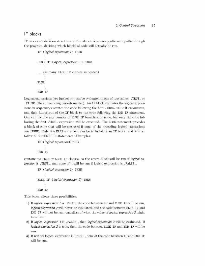
6. Control Structures 25
IF blocks
IF blocks are decision structures that make choices among alternate paths through
the program, deciding which blocks of code will actually be run.
IF (logical expression 1) THEN...
ELSE IF (logical expression 2 ) THEN...
. . . (as many ELSE IF clauses as needed)...
ELSE...
END IF
Logical expressions (see further on) can be evaluated to one of two values: .TRUE. or
.FALSE.(the surrounding periods matter). An IF block evaluates the logical expres-
sions in sequence, executes the code following the first .TRUE. value it encounters,
and then jumps out of the IF block to the code following the END IF statement.
One can include any number of ELSE IF branches, or none, but only the code fol-
lowing the first .TRUE. expression will be executed. The ELSE statement precedes
a block of code that will be executed if none of the preceding logical expressions
are .TRUE. Only one ELSE statement can be included in an IF block, and it must
follow all the ELSE IF statements. Examples:
IF (logical expression) THEN...
END IF
contains no ELSE or ELSE IF clauses, so the entire block will be run if logical ex-
pression is .TRUE., and none of it will be run if logical expression is .FALSE..
IF (logical expression 1) THEN...
ELSE IF (logical expression 2) THEN...
END IF
This block allows three possibilities:
1) If logical expression 1 is .TRUE., the code between IF and ELSE IF will be run,
logical expression 2 will never be evaluated, and the code between ELSE IF and
END IF will not be run regardless of what the value of logical expression 2 might
have been.
2) If logical expression 1 is .FALSE., then logical expression 2 will be evaluated. If
logical expression 2 is true, then the code between ELSE IF and END IF will be
run.
3) If neither logical expression is .TRUE., none of the code between IF and END IF
will be run.

26 I. Basic Elements of Fortran
IF (logical expression) THEN...
ELSE...
END IF
This block allows only two possibilities.
1) If logical expression is .TRUE., the code between IF and ELSE will be run.
2) If logical expression is .FALSE., the code between ELSE and END IF will run.
Single-statement IF— A simple IF block of the form
IF (logical expression) THEN
one executable statementEND IF
can be simplified by deleting the THEN and END IF, reducing the three-statement
block into a single statement:
IF (logical expression) one executable statement
Logical expressions
Logical expressions normally consist of comparisons in which one numeric value is
compared to another and found to be equal, not equal, greater than, and so forth,
or in which one character string is found to be equal or not equal to another. The
numeric logical operators consist of:
== equal to
/= not equal to
< less than
<= less than or equal to
> greater than
>= greater than or equal to
Each of the following poses a question to the computer, such as “Is a equal to
b?” in the first case or “Is i less than or equal to 100?” in the last case. If the
answer is yes, the expression takes on the value .TRUE.
a == b g > 0.0
ans == ’y’ i <= 100

6. Control Structures 27
Logical operators. Logical expressions and variables have a form of arithmetic
in which two logical variables or expressions can be compared using an operator,
producing a result that is also a logical expression or variable. Four of these are
considered “binary” operators, which in this context means that they act on two
values to produce a single value. The .NOT. operator is the logical equivalent of a
minus sign, changing the value of a single logical result to its opposite.
.AND. Logical “and”
.OR. Logical “or” (equivalent to “and/or” in normal language)
.NOT. Logical negation (change .TRUE. into .FALSE., and vice versa)
.EQV. Logical equivalence
.NEQV. Logical nonequivalence
Truth Table for Logical Operatorsk m k.AND.m k.OR.m k.EQV.m k.NEQV.m .NOT.k
.TRUE. .TRUE. .TRUE. .TRUE. .TRUE. .FALSE. .FALSE.
.TRUE. .FALSE. .FALSE. .TRUE. .FALSE. .TRUE. .FALSE.
.FALSE. .TRUE. .FALSE. .TRUE. .FALSE. .TRUE. .TRUE.
.FALSE. .FALSE. .FALSE. .FALSE. .TRUE. .FALSE. .TRUE.
Examples. The first example will be true only if a is between 0 and 1.
a > 0.0 .AND. a < 1.0
The next will be true if ans is either uppercase or lowercase “y”.:
ans == ’Y’ .OR. ans == ’y’
Occasionally a logical expression will be more clear if expressed with a negation,
but this is more often used with logical variables.
.NOT. a > b is logically equivalent to a <= b
Unlimited DO loop
The unlimited DO loop will continue forever, unless some condition causes an
EXIT, STOP, GO TO, or RETURN statement to be executed. (EXIT, STOP, and GO TO are
covered later in this chapter. RETURN is covered with SUBROUTINEs in Chapter 8.)
DO...
END DO
where code between the DO and END DO will be repeated indefinitely. Practical use
of this loop usually has an EXIT statement as part of an IF structure.
DO...
IF (logical expression) EXIT...
END DO

28 I. Basic Elements of Fortran
EXIT and CYCLE
EXIT and CYCLE break out of a DO loop temporarily or permanently. EXIT means
leave the loop: proceed with the first statement after the END DO, regardless of the
state of the counting variable or logical condition.
CYCLE means go back to the DO statement and make the next pass through the loop.
For example:
DO i=1,n...
IF (logical expression) CYCLE...
END DO
This loop will execute the top section for every pass through the loop, and it will
execute the bottom section each time that logical expression is .FALSE.
Direct Transfers
GO TO statement— unconditional transfer to another part of the scoping unit.
GO TO statement label
where statement label is a literal positive integer constant of five or fewer digits,
placed at the beginning of a Fortran statement to “label” the statement. Statement
labels do not have to refer to line number or be in increasing order, but they must
be unique within a scoping unit.
GO TO 100
requires that somewhere else in the scoping unit, there is a statement of the form
100 executable statement
and execution of the GO TO statement transfers control directly to the statement
labeled 100. Transfers may be forward or backward within a scoping unit.
Transfers cannot go into the range of a DO loop or IF block, so it is occasionally
useful to have an inactive executable statement to serve as a target. The CONTINUE
statement serves this purpose—it does nothing but tell the computer to move on
to the next line.
100 CONTINUE
could serve as the target of a GO TO 100 statement if it is inconvenient, confusing,
or illegal to label the beginning or end of a control structure block.
Fortran versions before Fortran 90 lacked EXIT, CYCLE, and unlimited DO loops,
so GO TO was a common statement. It is now seldom needed. Some coding styles
obsess on avoiding all GO TO statements. That paradigm can create ugly, contrived
use of control structures, in place of which a careful use of GO TO is preferable.
STOP statement— Stop execution and return to the environment that called the
program. Inclusion of a STOP statement is optional if it would be the last executable
statement of program because reaching an END PROGRAM statement implies a STOP
and returns control to the operating system.

7. Arrays
Arrays are collections of variables in which a single name refers to a whole list of
numbers (or character strings). Individual numbers within the array, or subsets
of the array, can be accessed by the combination of the array name and index
numbers that point to positions within the array. For example, instead of making
365 variable names to list all the temperatures in a year, we might declare an array
temperature that holds 365 numbers, and refer to the temperature on the 15th of
February as temperature(46), the 46th temperature in the array.
Any declared variable name becomes an array if provided with an index range,
as in the general declaration of a one-dimensional array:
type name, attributes :: symbolic name (lower bound:upper bound)
Index values (lower bound and upper bound) must be INTEGER constants in a
program. Commonly the lower bound is one and can then be omitted.
One-dimensional arrays with an implied lower bound of one are simplest to
understand—think of a list of items accessed by their numerical position on the list.
The following array declaration allocates one-dimensional REAL arrays with 10, 20,
16, and 201 elements, respectively.
REAL :: a(10), b(20), c(0:15), d(-100:100)
The first two are equivalent to declaring a(1:10) and b(1:20).
Fortran also allows for two-dimensional arrays, analogous to a table, three-
dimensional arrays, analogous to sheets of tables, and so on up to a maximum of
seven dimensions.
A list of arrays the same size may be declared using the DIMENSION attribute.
INTEGER, DIMENSION(20) :: a, b, c, d(10)
defines three arrays of size 20 and one array of size 10—the explicit dimension on d
overrides the DIMENSION attribute.
When declaring an array of character strings, the length of each string follows
the array declarations. The following two declarations are exactly the same:
CHARACTER :: station(100)*12
CHARACTER(LEN=12), DIMENSION(100) :: station
These both declare station to be an array consisting of 100 character strings, each
of which is 12 characters long.
Initialization, Literal Representation
Arrays can be initialized or made into constants, just as with scalars.
INTEGER, PARAMETER, DIMENSION(3) :: n=(/ 12, 32, 41 /)
REAL :: c(4) = (/ 1.0, 2.0, 3.0, 4.0 /)
In this example, n is a constant array that cannot be changed, whereas c can be
subsequently changed. Note the (/ . . . /) used to list elements of a one-dimensional
array—this is known as an array constructor. Arrays can also be initialized with
29

30 I. Basic Elements of Fortran
an implied DO loop. The following produces the same c array as the previous
example.
REAL :: c(4) = (/ (i, i=1,4) /)
Array References, Array Sections
An array reference may look the same as an item in a declaration statement, but in
an executable statement, an array name followed by integer numbers in parentheses
refers to individual array element or a range of array elements. For example,
WRITE (*,*) a(k), b(23)
will output two numbers: element k of a one-dimensional array a, and element 23
of a one-dimensional array b.
An array section might also look like an entity in a declaration statement, but
it will indicate a range of array elements using a colon to separate the first element
in the range from the last element in the range. If a is a one-dimensional array of
size 100, then
WRITE (*,*) a(1:10), a(91:100)
will write out the first 10 and last 10 numbers in the array.
Array Arithmetic
Any arithmetic expression in which one or more of the elements are arrays or array
sections will be applied elementwise to all the values in the array.
y = y + 2.0 * b
will work if y and b are scalars. If y and b are both arrays of length n, that single
statement is equivalent to
DO i=1,n
y(i) = y(i) + 2.0 * b(i)
END DO
If y and b were of different lengths greater than n, an expression equivalent to the
preceding loop, using explicit array sections, would be
y(1:n) = y(1:n) + 2.0 * b(1:n)
Intrinsic Functions used with Arrays
Elemental Functions. Most of the “calculator” functions will operate on arrays
correctly.
a(1:10) = SIN( b(1:10) )
will calculate 10 sine function values, one for each value in b(1:10), and store
the results in a(1:10). Functions that do array operations this way are called
elemental functions.

7. Arrays 31
Functions that Operate Only on Arrays. These functions perform array re-
ductions. Their arguments are arrays or array sections, but one number is returned
for the function value.
Sum of elements SUM( array )
Sum of product of elements DOT PRODUCT( vector1, vector2 )
Value of largest or smallest element MAXVAL, MINVAL( array )
Index of largest or smallest element MAXLOC, MINLOC( array )
(Result of MAXLOC or MINLOC is a one-dimensional integer array, whose dimen-
sion is the number of dimensions in the argument, and whose values are index
positions of largest or smallest element)

32 I. Basic Elements of Fortran
Array Example
PROGRAM Array Example
IMPLICIT NONE
INTEGER, PARAMETER :: n=10, k=2000
REAL :: a(n), b(k), c(n,k), d(k), e
! Declares three 1D arrays, one 2D array, and a scalarINTEGER :: i, j
OPEN (250,FILE="some.data")
DO i=1,k ! Reads k linesREAD (250,*) c(1:n,i) ! Reads n numbers from each line! Code implies that data file has at least k lines! and at least n numbers on each line.
END DO
DO i=1,n ! Loop range is first index range of c.! Next four lines are the summing algorithm, i does not change.a(i) = 0.0 ! Empty the bucketDO j=1,k ! Loop range is second index range of c.
a(i) = a(i) + c(i,j)
! References to single elements of a and c.END DO
END DO
! a is now a vector holding the sums across the second index of c.
! Previous nested DO loops could be replaced with one statement:
! a = SUM ( c, DIM=2 )
! or more explicitly! a(1:n) = SUM ( c(1:n,1:k), DIM=2 )
! Calculate b as sums across the 1st dimension of c.b = SUM ( c, DIM=1 )
e = MAXVAL ( b ) ! Single scalar answer: largest value in b.
d(1:k) = SQRT ( b(1:k) / e )
! SQRT is elemental: it creates a new value in d for each value in b/e
! Equivalently in a loop
! DO j=1,k
! d(j) = SQRT ( b(j) / e )
! END DO
OPEN (251,FILE= "silly.statistics")
WRITE (251,"(5F10.2)") d ! Writes out every value in d
! Format allows 5 values per line, takes as many lines as needed.STOP
END PROGRAM Array Example

8. Module Subroutines
“Scoping Units” is Fortran jargon for the parts of a program that hide some of their
internal variables and structure from each other. The scoping units in a modern
program are of type PROGRAM, SUBROUTINE, FUNCTION, or MODULE. Names of variables
are only defined within a scoping unit, and communication of variable names and
values between scoping units is controlled. Another feature of scoping units is that
they allow some parts of a program to be compiled independently from the rest of
the program, enabling the existence of subroutine libraries and large projects.
The only scoping unit introduced so far is the program, which begins with a
PROGRAM statement and ends with an END PROGRAM statement. A program can be
started from the operating system—it is the “highest level” Fortran unit. The other
three have varying purposes. User-defined functions are used in the same manner as
intrinsic functions, usually to calculate a single number from one or more arguments.
Subroutines can encapsulate an algorithm, process, or calculation method in a way
that the procedure can be applied to different data at different points.
Modules have multiple purposes, including holding data and providing an in-
terface “wrapper” around subroutines and functions.
Scoping units hide information from each other—variables in one scoping unit
are known to another scoping unit only if they communicate these values explicitly.
The selective hiding and sharing of information between scoping units is responsible
for their usefulness, but this also makes them perhaps the most difficult useful thing
to learn in Fortran. The basic discussion in this chapter will be restricted to the
module subroutine.
Subroutines and Modules
Subroutines take the algorithm for a procedure and separate it from the particular
data on which the procedure operates. A subroutine is run by executing a CALL
statement from another subroutine or from a program. Communication between the
subroutine and the calling program is via argument lists—a dummy argument list
on the SUBROUTINE statement and an actual argument list at the CALL statement.
A SUBROUTINE statement declares the name of a subroutine. It includes a symbolic
name for the routine and usually includes a dummy argument list in parentheses. A
SUBROUTINE statement is bracketed with an END SUBROUTINE statement, analogous
to the PROGRAM/END PROGRAM pair.
A subroutine is usually designed primarily for its executable statements —it
holds a pattern of executable statements, an algorithm. Each time the subroutine is
called, it performs its algorithm on a different set of data. Those data are primarily
communicated into the subroutine via the argument list.
A module is primarily designed around declarations. A module can be thought
of as a container that holds things: data objects such as constants and variables,
and executable procedures (functions and subroutines). The data and procedures
become available within any program or subprogram that invokes the module with
a USE statement. In our first examples, the module will be just a container for
a single subroutine, so its purpose may seem obscure simply because it does not
33

34 I. Basic Elements of Fortran
appear to do anything—it will just seem to be some extra statements bracketing
the subroutine.
This next block of code illustrates the pattern of statements that distinguish a
module subroutine from a program.
MODULE First Sub Wrapper
CONTAINS
SUBROUTINE First Sub ( dummy, argument, list )
IMPLICIT NONE
INTEGER, INTENT(IN) :: dummy
REAL, INTENT(INOUT) :: argument(:)
REAL, INTENT(OUT) :: list
REAL :: local, variable, lists
INTEGER, SAVE :: permanent, local vars... ! More declarations of local variables if needed.
! Executable code follows....
RETURN
END SUBROUTINE First Sub
END MODULE First Sub Wrapper
Code from the SUBROUTINE statement to the END SUBROUTINE statement mimics
the pattern of statements needed for a simple program. First, some declarations,
then some executable statements, then a RETURN takes the place of STOP. While
STOP restores execution control to the operating system, RETURN restores execution
control to the scoping unit that called this subroutine – either a program or another
subroutine.
A SUBROUTINE statement differs from a PROGRAM statement in the presence of a
list of dummy arguments. (A subroutine may have any number of such arguments,
or none at all.) These arguments are one means by which information is passed
between a subroutine and its calling program. In this example, dummy, argument,
and list are three variable names for which values may be received from or passed
back to the calling program. These need not have the same names as the same
variables in the calling program, just the same type, kind, rank, and they must
have attributes that are compatible with the INTENT attributes.
INTENT attributes. Because dummy arguments communicate with the calling
program, it is useful to define whether they are “input arguments” or “output
arguments.” These attributes may be applied only to dummy arguments only, thus
the separate declarations shown above for local variables.
In the example given above, dummy is INTENT(IN) and cannot, therefore, be
changed in this subroutine. Any attempt to use dummy in the input list of a READ
statement, the left side of a replacement statement, or as a DO variable should
be flagged by the compiler. It would also be illegal for this subroutine to call
another subroutine using dummy for any argument that did not have the INTENT(IN)
attribute within the called subroutine.
INTENT(OUT) implies that list will be modified and given a value by this
subroutine, and that this subroutine does not rely on list having a value when it
8. Module Subroutines 35
enters the subroutine. The compiler should flag any attempt to use list before
it is defined (for example, using it in the right side of a replacement statement
before it has been given a value in this subroutine). INTENT(INOUT) implies that a
dummy argument may be both used and changed, that information needed by the
subroutine will enter with that variable, but some or all of that information will be
changed on exit.
Assumed-Shape arrays. In the preceding subroutine example, argument is
declared with parentheses following the name as if it were a one-dimensional array.
However, the parentheses contain only a colon. The (:) declares that argument
will be a one-dimensional array. The size and bounds of the array can vary from call
to call, so they do not need to be declared explicitly here. If the subroutine needs to
know the size of the array, an intrinsic function is provided: SIZE(argument) gives
an integer result telling how many elements are in argument once the subroutine is
actually being run.
Local Variables and SAVE. In the preceding subroutine example, local, vari-
able, lists, permanent, and local vars, and any other variables declared along
with them, are local variables. Their values and names are known only within
this subroutine. The same names could be used in other scoping units in totally
different ways. (The term “scoping units” comes from this idea, that local variables
cannot be seen outside the local scope.) At the end of the subroutine’s executioon
when RETURN sends control back to the calling program, none of the information
contained in those variables is transmitted back to the calling program.
Local variables do not necessarily occupy permanent storage space. If local or
variable are given a value during one call of this subroutine, there is no guarantee
that value will still be there when the subroutine is called a second time in the same
program. Computers often make room for local variables in a pool of scratch space,
and between two calls to a given subroutine the computer may use that same scratch
space for another purpose. The second local variable declaration includes a SAVE
attribute, which requests that the compiler give some permanent (static) storage
space to these variables. The SAVE attribute ensures that the values of permanent
and local vars left behind on one call of this subroutine will still be there at the
beginning of the next call.

36 I. Basic Elements of Fortran
Calling a Subroutine
The previous section repeatedly discussed effects of calling a subroutine, so we are
overdue for showing how that happens.
PROGRAM Caller
USE First Sub Wrapper, ONLY : First Sub
IMPLICIT NONE
INTEGER, PARAMETER :: actual=12
REAL :: arg(100), arg2(actual), arg3(45), &
var, xvar... ! Values should be set in the arrays here.
CALL First Sub ( dummy=actual, argument=arg, list=var )
CALL First Sub ( dummy=actual, argument=arg2, list=xvar )
CALL First Sub ( dummy=actual, argument=arg3, list=var )...
STOP
END PROGRAM Caller
The module name appears in a USE statement, which is a declaration state-
ment, and the subroutine is invoked as many times as needed in an executable CALL
statement. Information and data are conveyed between the program and the sub-
routine using the actual argument list. Each of these major elements needs to be
dealt with in turn.
USE— A MODULE from which variables, constants, or subroutines will be needed
is invoked by the USE statement—a declaration statement. This statement must
be before any other declaration statements within the program or subroutine, i.e.,
it must be after the PROGRAM, SUBROUTINE, or FUNCTION statement that names the
subprogram and before the IMPLICIT NONE statement. The syntax can be simple:
USE module name
Unlike other declaration statements, only one MODULE may be named in a USE
statement—there can be more than one USE statement if more than one MODULE
is needed.
If a module contains more than one subroutine or variable, it is possible to
restrict access to the module to only the items that are needed by the program.
USE module name, ONLY : list of names needed from the module
That form was used in our example, even though First Sub Wrapper contains just
one item. The ONLY clause is optional, but it is recommended as a way of declaring
the source of the subroutine name. In large programs, any given program or sub-
routine may USE several modules, each of which defines a number of subroutines or
variables. The ONLY clause clarifies what subroutine comes from what module, so
it is a good habit even with simple cases like this.
CALL— The actual execution of a subroutine occurs when it is invoked in a CALL
statement with an actual argument list. Two different ways are used to specify
the actual argument list. In keyword form, the dummy argument names from the
subroutine being called are given and set equal to the actual argument name, as in

8. Module Subroutines 37
CALL subroutine name ( dummy=actual, argument=argument, list=list )
An alternative way is to list the actual arguments without keywords but in the same
order as the dummy arguments, establishing association by position in the list (first
dummy argument is replaced by first actual argument, and so on).
CALL subroutine name ( actual, argument, list )
When the CALL is executed, information is transferred by replacing the dummy
arguments in the SUBROUTINE statement with the actual arguments in the CALL
statement. Then, the executable statements in the subruoutine run as if the
dummy argument names have been all replaced by the corresponding actual ar-
gument names. (In some cases, the compiler may implement this literally, by giving
the subroutine addresses in the computer’s memory to the actual arguments. In
other cases, the subroutine has copies of the actual arguments, but the effect is the
same.)
The subroutine proceeds with all the usual rules for Fortran executable state-
ments. Any of the executable statements can be used by subroutine, including I/O
statements, replacement statements, all the control structures, and also CALL state-
ments to other subroutines. A subroutine may also execute a STOP statement to
leave the program and go back to the operating system. The usual way to leave a
subroutine, however, is via a return statement.
RETURN— When a RETURN statement is encountered in a subroutine, execution
control returns to where the subroutine was called. Since a subroutine may be called
from more than one place, the computer must keep track of which call statement is
being returned to. At that time, the information in the dummy arguments within
the subroutine must be conveyed back to the calling program. Whatever values the
dummy arguments had at the end of the subroutine execution, the corresponding
actual arguments will now have. Execution within the calling program resumes
with the statement after the CALL statement. A RETURN statement can appear only
in a SUBROUTINE or FUNCTION, never in a PROGRAM.
A Module Subroutine Example
MODULE Two Stats M
IMPLICIT NONE ! this applies to all CONTAINed proceduresCONTAINS
SUBROUTINE Two Stats (x, mean, sd) !3 dummy argumentsREAL, INTENT(IN) :: x(:) ! x is assumed shapeREAL, INTENT(OUT) :: mean, sd
! INTENTs indicate if an argument changes in this routine.
REAL :: n ! Local variable.
n = REAL ( SIZE(x)) ! SIZE: how many elements are in x.mean = SUM( x ) / n
sd = SQRT ( SUM ( (x - mean) ** 2 ) / n )
RETURN
END SUBROUTINE Two Stats
END MODULE Two Stats M

38 I. Basic Elements of Fortran
This module subroutine encapsulates two simple statistical definitions: that the
“mean” is the sum of a list of numbers divided by how many numbers are in the
list, and that the “standard deviation” is the square root of the mean squared
difference between the value of numbers in the list and the mean of those numbers.
The calculations required are contained in two executable statements.
The INTENT attributes are applied only to the dummy arguments. To a sub-
sequent user of this subroutine, they serve as a form of documentation, telling the
user which arguments will be changed (mean and sd) and which arguments will not
be changed (x). To the writer of the subroutine, they check whether the intentions
of the writer were carried out in the code: the compiler will generate error messages
for INTENT(IN) arguments that are changed by the subroutine and for INTENT(OUT)
arguments that are not defined within the subroutine.
The dummy argument list defines names that will be used within the routine.
The names used in the calling program need not be the same names, but they do
need to have the same purposes: a real array that has numbers on entering the
routine, and two real scalars that will become the mean and standard deviation of
the numbers within the array.
The IMPLICIT NONE statement in the module carries over to any subroutines
or functions contained within the module. However, it does not carry over to or
from the calling program.
The dummy argument x is an assumed-size array. The SIZE intrinsic function
was used to find out how many elements are actually in the array.
Argument Association
Argument association refers to the most important and difficult aspect of writing
and using subroutines: how to match actual arguments in a call statement with
dummy arguments in a subroutine statement. Imagine that the following program
makes use of the module subroutine on the previous page. Compilation of the
module can be separate from compilation of the calling program.
PROGRAM Driver
USE Two Stats M ! USE makes module available to program.IMPLICIT NONE
INTEGER, PARAMETER :: n=100, k=200
REAL :: a(n), b(k), a mean, a sd, b mean, b sd... ! Code to open a file and read values for a and b.
CALL Two Stats ( x=a, mean=a mean, sd=a sd )
CALL Two Stats ( x=b, sd=b sd, mean=b mean )... ! Code to write out a mean, a sd, b mean, and b sd.
STOP
END PROGRAM Driver
Dummy arguments in this example were the list (x, mean, sd) from the SUB-
ROUTINE statement. Dummy arguments are called that because they take up no
actual space—they are merely placeholders for actual values that will be inserted
when the subprogram is called.
Actual arguments in this example are the lists (a, a mean, a sd) and (b,

8. Module Subroutines 39
b mean, b sd). Because of use of the keyword form, in which dummy argument
names from the SUBROUTINE statement are associated literally with actual argument
names in the CALL statement, the order in which these actual arguments were spec-
ified is not important. For example, the first CALL statement above can be replaced
with the following:
CALL Two Stats ( mean=a mean, x=a, sd=a sd )
If these CALL statements were specified without the keywords, then only the order of
the actual arguments would determine their association with the dummy arguments.
A variable called n is declared in both Driver and Two Stats. Because it is not
communicated via the argument list, it is not the same variable in the two different
scoping units. Again, the name “scoping units” implies that a variable name and
value is only known within the “scope” of its particular unit unless specifically
communicated outside that unit.) n is a local variable within Two Stats.
Dummy arguments may be given the OPTIONAL attribute, in which case cor-
responding actual arguments may not need to be included. Writing a subroutine
with this feature requires careful use of the PRESENT intrinsic function.

II. Advanced FortranPart I covered a subset of Fortran sufficient for a large fraction of the small, scientist-
written programs needed for data analysis and model building in the environemntal
sciences. Some programmers may never need to go beyond the features already
covered, especially students learning Fortran only to learn programming principles
but expecting to use other languages and systems in later work.
Part II adds features and complexity to every aspect of the language. The
control structures and arithmetic syntax become more varied. Although every con-
ceivable algorithm can be expressed with the two DO loops, IF structures, GO TO,
and the ability to CALL and RETURN from subroutines, this part introduces SE-
LECT CASE, and another kind of DO loop, which make some algorithms easier to
understand and possibly more efficient. The FORALL structure may help multipro-
cessor computers distribute calculations over more than one processor. WHERE looks
like a control structure, but really is a way of bringing elemental array syntax to
decision structures in a way that the IF structures cannot handle.
Subroutines and modules have additional uses. Subroutines can be made
generic, so that more than one subroutine can be called by the same name, with
the compiler choosing the appropriate subroutine based on the type of the actual
arguments in the CALL statement. The section of the MODULE before its CONTAINS
statement will now become useful, and there will be modules that do not hold any
subroutines but are used entirely for their data-declaration capabilities. Also, we
will introduce another scoping unit that is best understood as a limited variation
on the subroutine, called the user-defined function.
Part II covers two remaining instrinsic types: LOGICAL and COMPLEX. Variables
can also be aggregated into groups that work together using the user-defined type
mechanism. Storage of arrays will become more flexible with the ability to ALLOCATE
and DEALLOCATE storage space at run time, or to use POINTER syntax.
Along the way, there will be a certain amount of repetition, because features
introduced in Part I will be given a short synopsis here, so that Part II is relatively
complete on its own.
40

9. Data Types
Computers, as we know them, store binary digits—no other kind of information.
The purpose of an operating system or programming language is to make dealing
with the binary digits easier for humans, primarily by organizing them into groups
that make sense as data objects. Fortran began as a general purpose language
(since it was the only one) but development of diverse other languages have made
it primarily a language for scientists and engineers. Fortran numeric types emulate
traditional scientific data: measurements of field variables, numbers that annotate
location, time, or experiment identifiers for such measurements. Fortran has enough
character string capability to deal with files and directories and to label things
properly, but is not really intended for a text manipulation application.
Fortran uses three intrinsic types for numerical information: REAL, INTEGER,
and COMPLEX; and two intrinsic types for nonnumeric information: CHARACTER
and LOGICAL. For most scientific programs: measurements and theoretical results
are REAL and very occasionally COMPLEX, labels and annotation necessary to keep
track of the size, purpose, and location of data are CHARACTER and INTEGER, and
algorithm control relies mostly on INTEGER and LOGICAL variables.
Those five types are the complete set of intrinsic types in Fortran. Besides
type, the attributes that describe a variable are kind and rank. Each type may
have more than one kind, although only the REAL and COMPLEX types are required to
have more than one kind. For the numeric types, KIND parameters may extend the
range or precision of the numbers that can be stored in the type, or alternatively
reduce the range while allowing more numbers to be stored in a smaller space. The
Fortran numeric types, REAL, COMPLEX, and INTEGER, are modeled on their math-
ematical namesakes, so they do not change their major characteristics when KIND
designations change. However, the major difference between a computational form
of these numbers and the mathematical idealization is that computer numbers are
limited to a finite subset of the mathematically infinite sets of numbers. Informa-
tion about KIND indicates what subset can be stored with a particular model for
allocating and interpreting binary digits within the computer.
Real numbers express the most important data in many Fortran programs, and
the default subset is often not sufficiently large or precise, particularly in numeri-
cal models where extra significant digits of precision are often necessary to ensure
numerically stable calculations. Fortran requires that a higher precision KIND be
available for REAL numbers, and by extension to COMPLEX numbers, which are just
stored as two REAL numbers representing the real and imaginary parts of a complex
number.
KIND information for CHARACTER data has a different function—usually chang-
ing the character set or alphabet used. The default character set must include all the
characters needed for Fortran programming and may include any other characters; a
common default character set is the ascii set presented in Appendix B. Characters
in different alphabets require different KIND parameters to access. Fortran stan-
dards do not require a compiler and system to provide any alternate character sets
beyond the default set, but a compiler vendor with an interest in an international
41

42 II. Advanced Fortran
market is likely to provide at least an extended version of ascii that includes the
most common European accented characters, and perhaps also a two-byte character
set, such as Unicode, will be available to represent tens of thousands of characters
and symbols from most of the worlds’s languages.
Fortran also has a derived type mechanism for combining variables into logi-
cally related groups. When a specific data value needs to be shown directly and
exactly in code, as a literal or constant value, the format depends on the type
of the data value. Similarly, the manner in which information is actually stored
in computer memory varies with data type. Defining how information is actually
stored is beyond the Fortran standard and up to computer designers and compiler
writers, but Fortran provides a number of intrinsic inquiry functions that enable
a programmer to at least find out how a type is stored.
Numeric Types.
INTEGER. Integers are whole numbers, positive or negative. They have a range
limited simply by how many binary digits (bits) are used to store them. If k bits
are used to store an integer, then the most common way of allocating those bits
allows for representing 2k−1 negative integers, 2k−1 − 1 positive integers, and zero,
adding up to 2k different integers. For a 32-bit (4-byte) integer, that translates to
a range of −2 147 483 648 to 2 147 483 647 (just remember ±2 billion).
Integers are extensively used for counts that are related to programming, such
as the number of passes through a loop or the number of elements in an array. In
data, integers represent intrinsically whole number annotations, such as location
codes, sample numbers, or time numbers (day, month, hour). Most physical mea-
surements are not represented as computer INTEGERs even if they are only known to
a whole number value, and some intrinsically integer numbers, such as dates, may
need to be represented as REAL in order to make some calculations reliable.
Declaration of Integers. Use the keyword INTEGER. KIND parameters can be
specified for INTEGER variables. As with KIND for REAL numbers, they can change
the amount of storage space used for each number, which affects the possible range
of the number. In many compilers, INTEGER kinds that specify smaller than default
amounts of storage are available, even down to the level of using a single byte for a
number.
Unlike with REAL, the Fortran standard does not require that more than one
KIND of integer is provided. In many programming contexts, such as array or
string indexing, DO-loop indexing, and I/O unit numbers, Fortran requires that
the integers used be of the default KIND. Given that restriction, KIND designations
are seldom needed or used for INTEGER variables, and many long programs (and old
programmers) have never used any INTEGER variables that were not default KIND.
INTEGER variables may be initialized with constants or arithmetic expressions
involving constants. Variables given the PARAMETER attribute must be initialized,
and they can be used in arithmetic for subsequent declarations. In this example,
nn is a constant that cannot be changed; a and b can be subsequently changed; c
and d do not yet have values; and e and f may have a different range from default
integers, depending on how a given processor defines a KIND value of 2.

9. Data Types 43
INTEGER, PARAMETER :: nh=20, nw=15, nn=nh*nw, ne=(nh-1)*(nw-1)
INTEGER :: a=10, b=2*nn, c, d, workspace=13*nn+nh*nw+37
INTEGER(KIND=2) :: e, f
Any variable name used in the right side of an initialization expression must have a
known value. Thus, the fact that nn is given the constant value 20 in the preceding
statement is necessary for nn to be used in the initialization of b.
Inquiry functions with INTEGER results may be useful in some initialization
expressions. This next expression will create two constants: imax holds the largest
positive value that can be stored in a default INTEGER variable, pr holds the KIND
parameter that can be used with REAL declarations (see below) to get variables that
are accurate to at least 12 digits of precision, and prl is a KIND value for INTEGER
declarations if at least 8 digit values may be needed.
INTEGER, PARAMETER :: imax=HUGE(1), &
pr=SELECTED REAL KIND(p=12), &
prl=SELECTED INT KIND(p=6)
Literal Representation of Integers: Digits only, optionally with sign. A
decimal point must not be included. KIND parameters may be included.
0, 12345, -25, 3407 2, 120683 prl
in which the fourth number is 3407, to be stored as an integer of KIND parameter
2 and the fifth is 120683 to be stored with whatever KIND parameter is defined in
prl. In this usage, prl must have some constant, known value—such as would be
created by the initialization in the preceding example.
BOZ constants are means of expressing an integer value in a number base other
than decimal (base 10). Nondecimal integers can be used in very limited contexts,
primarily as actual arguments to numeric type conversion functions such as INT.
The other bases are binary (base 2) using the digits 0 and 1 with an indicator letter
B, octal (base 8) using the digits 0 through 7 with indicator letter O (letter O, not
zero), and hexadecimal (base 16) using the digits 0 through F (“digits” A through F
represent 10 through 15) with indicator letter Z. The following declaration initializes
all four variables to the same INTEGER value.
INTEGER :: i=INT(B’101101’), j=INT(O’55’), k=INT(Z’2D’), l=45
REAL. Most physical or scientific measurements will have characteristics of the
mathematical set of real numbers. In theory, any such measurement can have infinite
precision, and two different measurements can be infinitesimally close together. In
practice, any measurement we make has a limited degree of precision and range, and
two measurements that are too similar to be resolved as different by our instruments
will be considered the same. The Fortran type REAL is a finite approximation of the
infinite set of reals that operates in a similar manner: we are limited in precision,
resolution, and range compared to the mathematical set of real numbers.
A portion of the computer memory storing a REAL number is used to store an
exponent as a power of a known base, along with a multiplier, or fraction part,
that conveys the significant digits for that base. Using a 10-digit decimal calculator

44 II. Advanced Fortran
display as an example, a 10-digit integer could be stored exactly (numbers from
−1010 to 1010. However, allocating 8 digits to the multiplier and 2 digits to the
power of ten (exponent) we can now store numbers in the range ±10100 and can
handle numbers as small as 10−100 before they are indistinguishable from zero.
Each number is now only accurate to 8 digits. Ten digits can only distinguish
1010 different numbers, so any increase in range must come at a cost of decreased
precision.
The specific scheme by which binary digits are allocated among fraction, ex-
ponent, and sign values is called a number model. Each KIND of a numeric type
defines both a number of binary digits used to represent that KIND and a number
model for turning the binary digits into a number.
A common computer implementation for storing a REAL number in 32 binary
digits uses 8 bits for the exponent, which is a power of 2 in this context, and 24 bits
for the fraction part. Since 224 is about 16 million, only 16 million different fraction
multipliers can be stored. Allowing for positive and negative numbers, these real
number can only have a guaranteed precision of 6 digits. The range is controlled
by the 8 bits in the exponent: 28 is 256, and 2256 is about 1077. Those available
magnitudes are usually spread evenly around one (100), so that numbers whose
magnitudes range from 10−38 to 1038 can be stored with this number model. Neither
6 digits of precision nor a range of 10±38 is sufficient for many numerical calculations
needed in science—thus the need for a KIND that supports more precision and range
for REAL numbers by using more binary digits.
The most common long precision REAL number scheme uses 64 bits (8 bytes) for
each number, with 11 bits for the exponent and 53 bits for the fraction part. This
allows 253.= 9 × 10¹⁵ different fractions, or nearly but not quite 16 digit precision,
and an exponent range of 2211 .
= 10616 which is distributed on the range 10−308 to
10308. This KIND is widely used for numerical modeling. A “quad” precision using
128 bits (16 bytes) is also commonly available.
Literal representation of Real: The REAL numbers may have quite a compli-
cated representation, such as:
-1.234567E+28 8
which represents −1.234567×10+28 stored using a KIND of 8. The KIND designation
is required only if the default KIND is not used (but it is always allowed and often
preferred), + signs are always assumed if not included, and a number with magni-
tude conveniently near to one can be represented without the E notation. However,
the decimal point is always required to distinguish a REAL constant from an integer
constant. There must not be a decimal point on the exponent.

9. Data Types 45
Even if a value is a whole number, it must have a decimal point to be stored
in the real format. If a decimal point is attached, as in x = 2. * y, the decimal
indicates that the constant is a REAL number that happens to be a whole number,
not an INTEGER. Adding a decimal point to any constant this way changes the way
a number is stored and used for calculation.
Declaring Real Variables: The keyword is REAL, the attributes can include
a KIND designation, the PARAMETER attribute, a DIMENSION attribute for arrays
(Chapter 7 and 11), and designations for dynamic memory handling discussed later:
ALLOCATABLE, SAVE, TARGET, and POINTER. For a few simple scalars without initial-
ization:
REAL :: density, pressure, height
which declares three real numbers and assigns them variable names, but specifies
no values. An initial value can be provided for some or all of them within the
declaration:
REAL :: t=0.0, t0=15.0, a(4)=(/1.2, 0.3, -1.25, 1.78E-4/)
These initial values can be changed later in the program by READ or assignment
statements. If you have a number that should never be changed, include the PA-
RAMETER attribute.
REAL, PARAMETER :: epsilon=0.622, r=8314.3
These two variables can never be changed, and any attempt to change them later
in the program will produce an error message.
Precision and KIND. The range and precision of REAL numbers stored in various
standard schemes involving four or eight bytes was discussed earlier in this chapter.
Note that those typical ranges are not part of Fortran, but part of another comput-
ing standard (IEEE 754) that discusses number storage as used in many different
computer languages. Commonly, but again not standard or universal, is that the
KIND parameter will be the number of bytes used to store the number, so that 32,
64, and 128 bit numbers can be requested, respectively, with
REAL(KIND=4) :: x, y, z
REAL(KIND=8) :: a, b, c
REAL(KIND=16) :: u, v, w
The intrinsic function SELECTED REAL KIND finds KIND parameters for programs
that may need to run on more than one system. The intrinsic functions RANGE,
PRECISION, HUGE, TINY, and EPSILON find the accuracy and limits of each KIND.
To store a number at long precision, or to force a particular precision for a
literal constant, include a KIND parameter on the constant. In the following cases,
the 8 or 16 are not part of the number, but force the number to be stored using the
indicated KIND. Old-style “double precision” (KIND=8) can alternatively be indicated
using a D exponent instead of an E exponent. The last two numbers shown below
would be the same on a system for which (KIND=8) and DOUBLE PRECISION are the
same.
1.0 8, 3.141592654 16, 5.67E-12 8, 5.67D-12

46 II. Advanced Fortran
COMPLEX. A mathematical field of complex numbers consists of two real num-
bers stored under a single name representing the real and imaginary parts of a
complex number. In mathematics they may be represented as
z = x+ iy
in which x and y are both real numbers, i is the imaginary unit, i =√−1, and z is
the resulting complex number. In this representation, x is the real component and
y is the imaginary component. Complex numbers are essential to certain areas of
applied mathematics, such as time series analysis, wave propagation, or other areas
in which cyclic or repetitive processes must be studied. They also are needed as
eigenvalues in linear algebra so that all the roots of a polynomial equation can be
found, regardless of whether those roots are real.
Fortran provides a type COMPLEX that operates similarly by combining two
REAL numbers. Programming with Fortran’s COMPLEX type requires familiarity with
complex numbers. However, even a beginning user of Fortran will find references
to COMPLEX in mathematical libraries.
Declaration of complex numbers. Use the keyword COMPLEX; all other aspects
are the same as for REAL. The declaration may control the precision with KIND, set
a constant value with PARAMETER, or declare arrays of complex numbers using any
of the methods discussed for REAL data. KIND specifications for the COMPLEX type
are the same as the KIND specifications of the corresponding two REAL numbers, so
a COMPLEX(KIND=8) number consists of two REAL(KIND=8) numbers.
Literal representation of complex numbers: Two numbers, in the style of a
Fortran REAL, separated by a comma, inside parentheses. The first number is the
real component and the second is the imaginary component. The second example
below is still a complex number as stored in the computer, even though its imaginary
component is zero.
(1.0, 2.0) (50.1, 0.0) (12.2 8, 13.0 8)
The third example shows that KIND parameters may be specified individually for
the two components. If different KIND values are specified for the two components,
the computer will convert the lesser-precision component to be stored with the
same KIND as the higher-precision component—a processor will not store a COMPLEX
number with two different component KIND values.
Complex arithmetic: Complex numbers are more than just a pair of real num-
bers, they are a higher-order object than a real number. Although we can think
of a complex number as two real numbers, some of the arithmetic operations on
complex make more sense if a complex number is thought of in polar form with
a magnitude and a direction—a two-dimensional vector. Although Fortran does
not directly provide for such a representation, its implementation of the arithmetic
operations is correct for complex numbers, and is much different from simply apply-
ing arithmetic operations individually to corresponding components. Many of the
intrinsic functions (trigonometry, logarithms, etc.) have versions that will correctly
provide complex output if given complex arguments. As with complex arithmetic,

9. Data Types 47
these functions produce results that are very different from just applying the func-
tion to the individual component real numbers. Essentially, anyone not trained in
use of complex numbers should not assume they can correctly use the Fortran type,
but anyone familiar with complex numbers will find that the Fortran type works
naturally and intuitively similar to the mathematical complex field, with the usual
limitations on precision and range.
NonNumeric Types.
CHARACTER—Character strings consist of one or more letters, digits, or special
characters that can be represented by code numbers (known as a collating sequence).
Character strings may use a different character set than the simple set used for
Fortran code—the exact list varies with system and compiler. The most common
American implementation is the character set called ascii, which includes all the
Fortran characters plus special characters and action characters, such as linefeed
and backspace (see Appendix B).
With Fortran and English, this limited set of 128 ascii characters will usually
suffice. Extended ascii contains an additional 128 characters, including accented
characters for the most widely used European languages. For languages not based
on the roman alphabet, a character set called Unicode allows two-byte (16 bit) codes
for each character, giving a potential set of 65 536 characters. These cover the entire
range of the alphabetic languages of the world, a huge list of mathematical symbols,
and tens of thousands of symbols for Asian languages. Some systems and compilers
can handle Unicode characters in CHARACTER data, using KIND parameters to indi-
cate different character sets. There are other single-byte and multibyte character
systems besides ascii and Unicode.
Literal Representation of Character Strings: Enclose the string in apostro-
phes. Blank spaces and capitalization matter inside character strings. Apostrophes
are character string delimiters, not included in the string. Double quotation marks
may be used alternatively, but must be consistent: a particular string cannot be
started with an apostrophe and ended with a double quotation mark. (To indi-
cate an apostrophe inside an apostrophe-delimited character string, type it twice
together.)
’Fred’, "temperature", ’6’’ under’, ’2.54’
The last item is a four-character string, not a real number. It would be represented
in the computer by the character codes for the three digits and the decimal point,
and the computer would not understand it as something to do arithmetic on.
Declaration of Character strings: The keyword is CHARACTER. Lengths may
be declared for the entire statement using a LEN parameter or for individual names.
For example
CHARACTER(LEN=5) :: month, day, year
declares three character strings that are each 5 characters long, whereas
CHARACTER :: hour*4, station*12, time*7, inland

48 II. Advanced Fortran
declares four character strings that respectively contain 4, 12, 7, and 1 characters.
(No length designation implies a length of 1 character.) LEN parameters may be of
any length from 0 to a processor-dependent maximum. Many processors specify no
limit other than the maximum default INTEGER size as maximum length. Character
strings may have the PARAMETER attribute, and character strings may be initialized,
as with other data types.
Collating sequence. Every character set is really manipulated as a set of integer
codes. These codes are turned into graphical symbols with the familiar appearances
(the glyphs) only when needed—most of the time only the codes are stored. Even
when Fortran writes a text line to the screen, it only sends a set of numerical codes,
and it is the responsibility of other software or utilities to translate these codes into
glyphs.
Fortran restricts the order in which character codes are specified as follows:
the alphabetic characters A–Z must be specified in lowest to highest order, the
lowercase characters a–z must be also be specified in lowest to highest order, the
digits 0–9 must be specified in lowest to highest order, and the blank space must
be specified before any letters or digits. The ascii sequence in Appendix B is an
example of a collating sequence that satisfies these constraints. The purpose of
these constraints is simple: if you compare one character string to another using
the “lexical” comparison functions, you can put strings into alphabetical order. The
intrinsic functions LGE, LGT, LLE, and LLT perform these comparisons (see Ap-
pendix A). Lexical sorting operates on the character codes of the collating sequence,
so the standard guarantees that letters and digits will be sorted in the normal way.
The collating sequence rules of Fortran do not restrict the order of lowercase
letters relative to uppercase letters, nor do they specify the order of letters relative
to digits. Letters need not be adjacent—the code for B must be greater than the
code for A, but it does not have to be one more than the code for A. Similarly, the
positions of all the other Fortran characters are unspecified in the standard. Hence,
programs that rely on a particular collating sequence can be standard-conforming
but produce different results on different machines. The ascii collating sequence
is a popular choice for processors, but it is not universal. It is sufficiently popular
that the intrinsic functions IACHAR and ACHAR must be provided to reference ascii
even if it is not the collating sequence of that particular processor. If a program
requires use of a specific ascii code or reference to precise characteristics of the
ascii collating sequence, this usage should be carefully documented.
LOGICAL. Logical variables may only take on the two values .TRUE. or .FALSE.
to store a logical value for later tests. This type gets used quite differently from the
other intrinsic types, because assignment and testing of a LOGICAL variable are less
common than use of logical “arithmetic” within IF constructs.
Literal Representation of Logical : .TRUE. or .FALSE., that’s it. (The dots on
each side of the constants are necessary. As always, character case can be upper,
lower, or mixed in any way.)
Declaration of Logical: The keyword is LOGICAL, initialization is allowed, as is
the PARAMETER attribute and use of arrays. LOGICAL variables are normally stored

9. Data Types 49
in a default REAL sized space for storage efficiency even though only two values
are possible. Systems are allowed to offer alternate storage schemes using KIND
parameters, but sightings of such usage are extremely rare.
LOGICAL :: transient, ill conditioned, extra print=.FALSE.
LOGICAL, PARAMETER :: testing=.TRUE.
After these declarations, we have two uninitialized variables, a variable whose initial
value is given as .FALSE., and a constant. A logical parameter that causes every
IF test on that value to either fail or pass, without exception may seem pointless,
but the name suggests an application.
IF (testing) WRITE (test log,*) ’k after block 3’, k
provides a means of writing a long series of messages and values to a file during
testing. Since testing is a parameter, the only way to turn it off is to change
its value to .FALSE. in the declaration statement and recompile, at which point
a good optimizing compiler might recognize that the WRITE statements can never
be executed and completely eliminate their code from the compiled program. (One
should never second-guess what a compiler is actually doing, but it is best to provide
it as much information as possible.)
Other uses of LOGICAL variables are suggested by the other variable names. A
model that has both a steady-state and a transient mode, for example, may need
to test that in many places, such as output, boundary condition modification, and
equation setup. Setting a flag variable once, such as
transient = ctrans >= 1 .AND. ntimes > 0
followed by using direct tests such as
IF (transient) THEN
will generally be clearer than having to carry along and test ctrans and ntimes at
various locations.
Logical Arithmetic: In the introductory chapters, a discussion of “Logical Ex-
pressions” was included in the Control Structures section with the IF structure.
That reflects the fact that logical expressions are completely associated with the
IF statement in elementary programming. That section covers most of what needs
to be known about the topic, but the logical expression syntax is also a form of
arithmetic that can produce a logical result from two numeric values or from two
logical values. The operators fall into these groups:
Numeric logical operators (== /= < > <= >= ) appear between two numeric
values of the same type, turning the two numeric values into a single logical result.
For example, in a > b, both a and b must be INTEGER or REAL and the result of
the expression is .TRUE. or .FALSE.
The equality test operators == and /= may also be used with CHARACTER strings
and COMPLEX numbers. Some processors allow the “greater than” and “less than”
operators to be used with character strings for lexical comparisons as well, but
this is nonstandard and should be avoided. The lexical comparison functions, LGT,

50 II. Advanced Fortran
LGE, LLE, and LLT are provided for that purpose. Similar comparisons are math-
ematically undefined for COMPLEX numbers.
Logical comparison operators (.AND. .OR. .EQV. .NEQV) compare two logical
values and turns the result into a logical result—see the truth table in Chapter 6 for
their effects. A common usage would be to determine if a number is between two
boundary numbers without knowing which of the two boundary numbers is higher.
x > p(i) .NEQV. x > p(i+1)
In this example, if x is less than both p(i) and p(i+1), then both of the arithmetic-
logical comparisons will be .FALSE., so they are equivalent, and the compound
statement is .FALSE.. If x is greater than both p(i) and p(i+1), then both of the
arithmetic-logical comparisons will be .TRUE., so they are also equivalent, and the
compound statement is again .FALSE.. However, is x is between p(i) and p(i+1),
then one side of the compound statement will be .FALSE., the other side will be
.TRUE., and the .NEQV comparison (“not equivalent”) will make the compound
statement .TRUE..
Logical negation (.NOT.) is used as a “minus sign” on a logical expression or
variable. If the transient variable needed to be used in a positive test for steady-
state conditions, the test would be
IF (.NOT.transient) THEN
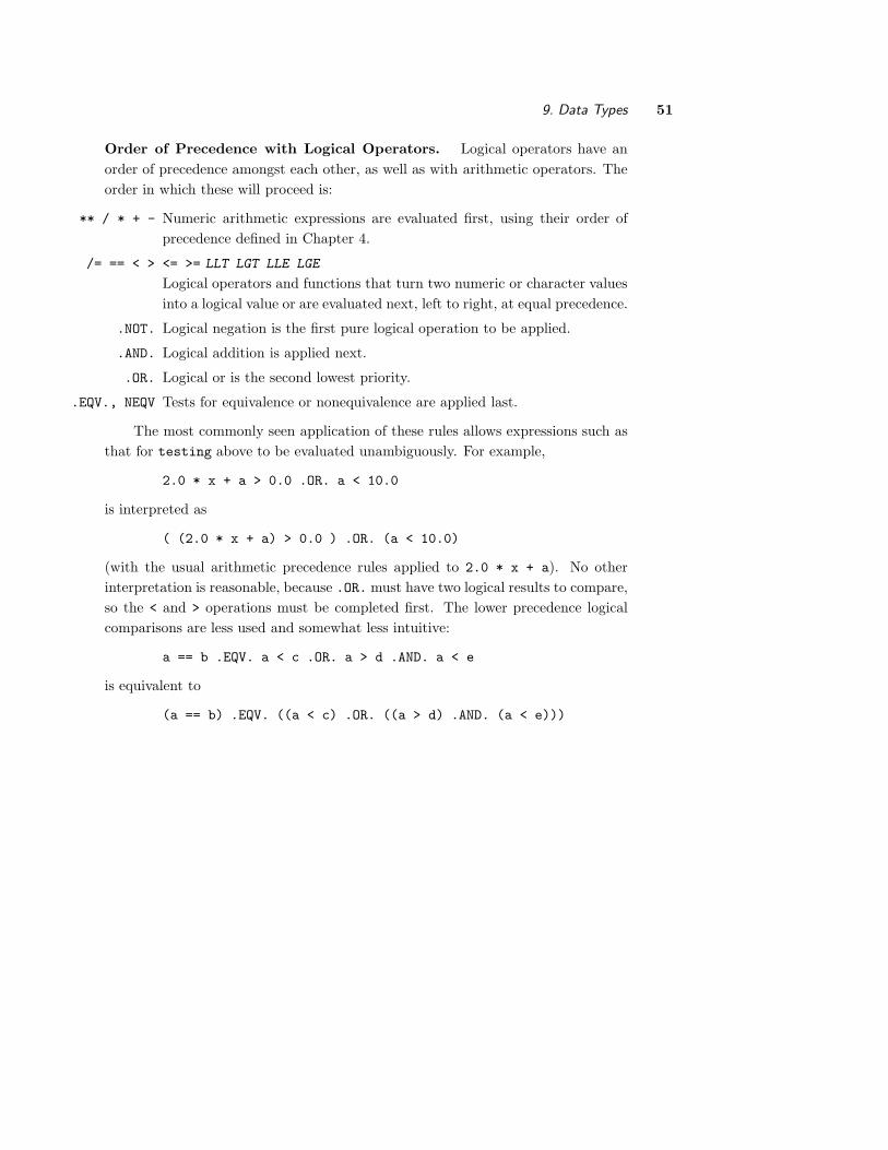
9. Data Types 51
Order of Precedence with Logical Operators. Logical operators have an
order of precedence amongst each other, as well as with arithmetic operators. The
order in which these will proceed is:
** / * + - Numeric arithmetic expressions are evaluated first, using their order of
precedence defined in Chapter 4.
/= == < > <= >= LLT LGT LLE LGE
Logical operators and functions that turn two numeric or character values
into a logical value or are evaluated next, left to right, at equal precedence.
.NOT. Logical negation is the first pure logical operation to be applied.
.AND. Logical addition is applied next.
.OR. Logical or is the second lowest priority.
.EQV., NEQV Tests for equivalence or nonequivalence are applied last.
The most commonly seen application of these rules allows expressions such as
that for testing above to be evaluated unambiguously. For example,
2.0 * x + a > 0.0 .OR. a < 10.0
is interpreted as
( (2.0 * x + a) > 0.0 ) .OR. (a < 10.0)
(with the usual arithmetic precedence rules applied to 2.0 * x + a). No other
interpretation is reasonable, because .OR. must have two logical results to compare,
so the < and > operations must be completed first. The lower precedence logical
comparisons are less used and somewhat less intuitive:
a == b .EQV. a < c .OR. a > d .AND. a < e
is equivalent to
(a == b) .EQV. ((a < c) .OR. ((a > d) .AND. (a < e)))

10. Input/OutputInput/Output (I/O) refers to all processes by which the computer communicates
with its environment. For this purpose the “environment” consists of keyboards, ter-
minal screens, permanent memory systems (magnetic disks, tapes, optical drives),
printers, and other devices that turn digital information into sound, pictures, pro-
cess controls, or instructions to any machine. The “computer” is the processing
unit that does arithmetic and logical operations and its high-speed, volatile mem-
ory systems: random-access memory and the cache. Fortran deliberately maintains
minimal control of hardware systems. An operating system that allocates virtual
memory on disk space or uses RAM as temporary scratch files is operating just
fine within the rules of Fortran. A programmer’s job is to allocate data space in
variables and arrays, and to define files that can be accessed via I/O commands.
The compiler and operating system working together as a “processor” decide where
to actually put things.
The transfer commands READ and WRITE make sense as verbs from the com-
puter’s point of view: READ causes input to the computer, WRITE causes output
from the computer. The other I/O statements control what device is being read to
or written from, what position to read from if the device is a file, and what kind
of translation to do between the binary information that computers use and the
formatted characters that humans can read.
READ statements
READ brings information into the computer from an external device, generally un-
derstood as input. A simple form is
READ (UNIT=unit number, FMT=format information) input list
where unit number is any nonnegative integer, format information is discused below,
and input list is a list of variable names that can be filled with information from the
external source that is being read. The unit number indicates which file, device,
or location that the computer is communicating with—see the OPEN statement.
Variables in the input list will be changed by the READ process, so they must be
unrestricted variables: they cannot be PARAMETERs, DO indexes, or literal constants.
(In most I/O statements, the UNIT= and FMT= keywords can be left out, but none
of the other optional keywords can be left out.) For example:
READ (5,*) time, date
says that two numbers should be read from unit number 5 in the default * format,
and these two numbers should be stored in the variable names time and date. Those
two variable names must have been previously declared, they must not be constants
with the PARAMETER attribute, and any previous information they contained will be
discarded to make room for the new input.
52
10. Input/Output 53
IOSTAT and END options. Either IOSTAT or END= options can control execu-
tion after reading an end-of-file marker.
READ (UNIT=10,FMT=*,IOSTAT=j) input listIF (j /= 0) EXIT
IOSTAT is a Fortran keyword, and j is any integer variable. If the READ statement
executes normally, j will be set to a value of zero, but if the READ statement tries
to read past the end of a file, j will be set less than zero. Another option in READ
accomplishes the same thing.
READ (UNIT=11,FMT=*,END=20) input list
In this case, trying to read the end-of-file mark causes execution to jump to a
statement labeled 20. (See GO TO for a discussion of statement labels.) This is
equivalent to the two-line form:
READ (UNIT=10,FMT=*,IOSTAT=j) input list
IF (j /= 0) GO TO 20
Both of these constructs are useful for reading a file into an array when the size of
the file (number of lines) is not known in advance.
INTEGER, PARAMETER :: nm=literal valueINTEGER :: a(nm), n, eof
...
DO n=1,nm
READ (10,*,IOSTAT=eof) a(n) ! eof is an integer variable.IF (eof /= 0) GO TO 20
END DO
WRITE (*,*) ’Warning about exceeding data capacity’
20 n = n - 1 ! n is now the number of lines actually read.
The IOSTAT value returned is mostly, but not completely, system dependent.
Portable Fortran programs rely on only three possibilities: zero indicates that the
READ statement was completed without error, a negative value indicates that an
attempt was made to read past the end of a file, and a positive value indicates
that some other kind of error occurred. Such “other” errors might include reading
characters of the wrong type, such as trying to read letters into a numeric value
or decimal points into an INTEGER value. The exact values and meanings of such
codes will be available in documentation for a specific processor and may be very
useful for debugging.
More options for READ statements.
READ (UNIT=unit number, FMT=format information, IOSTAT=status code,&REC= record number, &
ADVANCE= ’yes’ or ’no’, &
SIZE= number of characters, &
NML= namelist group )
REC allows specification of a particular record number for direct access input.
Direct access is discussed in more detail under the OPEN statement.

54 II. Advanced Fortran
ADVANCE by default is ’yes’, meaning that the file position pointer moves down one
line after a READ statement is executed, even if the entire line has not been
read. Changing to ’no’ can stop the file position pointer in mid line.
SIZE specifies how many characters should be read into a line when ADVANCE=’no’
is specified.
NML invokes a type of input that is different from both direct access and se-
quential access called namelist input, discussed later in this chapter.
WRITE
WRITE controls output of information from the computer to an external device.
WRITE (UNIT=unit number, FMT=format information) output list
output list is more flexible than input list, because information in the output list is
not changed by the WRITE process. Thus, PARAMETERs and literal constants may be
included. In the following, ’The answer is ’ is a literal character constant.
WRITE (UNIT=3,FMT=*) ’The answer is ’, x
More options for WRITE statements.
WRITE (UNIT=unit number, FMT=format information, IOSTAT=status code,&REC= record number, &
ADVANCE= ’yes’ or ’no’, &
NML= namelist group )
The descriptions of these under the READ statement can be reinterpreted directly
for output files.
OPEN
OPEN connects a file (or other device) to a particular unit number.
OPEN (UNIT=unit number, FILE=file name)
file name is a character string, specified either as a literal character string or as a
character variable. Its exact nature will vary with the operating system being used.
On Unix, it may include a complete or partial path. Examples:
OPEN (UNIT=3,FILE=’census.data’)
OPEN (UNIT=12,FILE=’/home/census/2010/delaware/sussex.data’)
OPEN (UNIT=27,FILE=’hcn/07/dailytemp.csv’)
CHARACTER(LEN=20) :: censusfile
READ (UNIT=*,FMT=*) censusfile
OPEN (UNIT=3,FILE=censusfile)
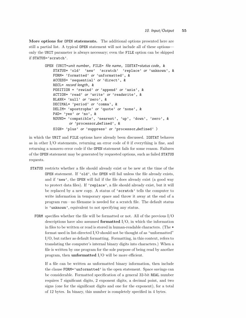
10. Input/Output 55
More options for OPEN statements. The additional options presented here are
still a partial list. A typical OPEN statement will not include all of these options—
only the UNIT parameter is always necessary; even the FILE option can be skipped
if STATUS=’scratch’.
OPEN (UNIT=unit number, FILE= file name, IOSTAT=status code, &
STATUS= ’old’ ’new’ ’scratch’ ’replace’ or ’unknown’, &
FORM= ’formatted’ or ’unformatted’, &
ACCESS= ’sequential’ or ’direct’, &
RECL= record length, &
POSITION = ’rewind’ or ’append’ or ’asis’, &
ACTION= ’read’ or ’write’ or ’readwrite’, &
BLANK= ’null’ or ’zero’, &
DECIMAL= ’period’ or ’comma’, &
DELIM= ’apostrophe’ or ’quote’ or ’none’, &
PAD= ’yes’ or ’no’, &
ROUND= ’compatible’, ’nearest’, ’up’, ’down’, ’zero’, &
or ’processor defined’, &
SIGN= ’plus’ or ’suppress’ or ’processor defined’ )
in which the UNIT and FILE options have already been discussed. IOSTAT behaves
as in other I/O statements, returning an error code of 0 if everything is fine, and
returning a nonzero error code if the OPEN statement fails for some reason. Failures
of the OPEN statement may be generated by requested options, such as failed STATUS
requests.
STATUS restricts whether a file should already exist or be new at the time of the
OPEN statement. If ’old’, the OPEN will fail unless the file already exists,
and if ’new’, the OPEN will fail if the file does already exist (a good way
to protect data files). If ’replace’, a file should already exist, but it will
be replaced by a new copy. A status of ’scratch’ tells the computer to
write information in temporary space and throw it away at the end of a
program run—no filename is needed for a scratch file. The default status
is ’unknown’, equivalent to not specifying any status.
FORM specifies whether the file will be formatted or not. All of the previous I/O
descriptions have also assumed formatted I/O, in which the information
in files to be written or read is stored in human-readable characters. (The *
format used in list-directed I/O should not be thought of as “unformatted”
I/O, but rather as default formatting. Formatting, in this context, refers to
translating the computer’s internal binary digits into characters.) When a
file is written by one program for the sole purpose of being read by another
program, then unformatted I/O will be more efficient.
If a file can be written as unformatted binary information, then include
the clause FORM=’unformatted’ in the open statement. Space savings can
be considerable. Formatted specification of a general 32-bit REAL number
requires 7 significant digits, 2 exponent digits, a decimal point, and two
signs (one for the significant digits and one for the exponent), for a total
of 12 bytes. In binary, this number is completely specified in 4 bytes.

56 II. Advanced Fortran
Unformatted I/O requires file documentation, as the contents of a file,
once written, can not be deduced from looking at the file, nor can a file
be easily read without knowing the WRITE statements that produced it.
Storage of binary information at varies among computer systems and is
not controlled by the Fortran standard. Writing a file on one system that
will be read later on the same system or one exactly it is seldom a problem.
ACCESS may be ’sequential’ indicating that input or output proceeds one line
at a time—each READ statement starts a new line, each WRITE statement
moves down to start on the next line. That is the default behavior.
If ACCESS is ’direct’, then each READ or WRITE statement to that unit
number must have a REC= specifier to indicate which record number (line
number) will be read or written by the statment. Direct access requires
that the RECL= option (below) is also specified.
RECL specifies as an integer the number of bytes in each record (or number of
characters in each line) of a direct access file. This is only needed for direct
access, as the length of each line must be the same so that computer can
calculate the position of any specified line number.
Note that if direct access is combined with unformatted data, the number
of bytes written on a line is the same as the number of bytes used to store
the variables internally. Thus, for systems in which the KIND values are
the number of bytes of memory used to store a variable, an unformatted
line requires 4 bytes for each KIND=4 REAL or INTEGER number, or 8 bytes
for each KIND=8 number.
POSITION makes sense only when opening an existing sequential access file. The
default is ’asis’ (read “as is”), in which the file position marker will be
at the beginning of the file for a file that has not been previously connected
in this Fortran program. Using ’rewind’ can force a file position marker
to the beginning, even if it has been partially read or written already in
the program. Use of ’append’ allows additional information to be added
to the end of a file that already exists.
ACTION can protect a file by restricting the I/O statements that can act on the file.
ACTION=’read’will prevent a unit number from having a WRITE statement
act on it. ACTION=’write’ will prevent a unit number from having a READ
statement act on it. ACTION=’readwrite’ allows everything.
BLANK controls whether blank spaces are treated as nulls (default) or zeros. Over-
rideable by edit descriptors BN and BZ.
DECIMAL controls whether the decimal point character is a period (default) or a
comma. Overrideable by edit descriptors DC and DP.
DELIM controls whether to output character strings in list-directed or namelist
output with no delimiter (default) or to use apostrophe (’) or quotation
mark (") delimiters.

10. Input/Output 57
PAD controls whether records that are shorter than needed for the input list
are assumed to have enough blank spaces to fill the input list (default) or
not.
ROUND sets the rounding mode. Overrideable by edit descriptors RU, RD, RZ, RN,
RC, and RP (rounding modes are described with those edit descriptors). No
default is specified by the standard.
SIGN controls whether numeric output of positive numbers includes a plus sign.
Overrideable by edit descriptors S, SS, and SP. Default is ’processor defined’.
A direct access example. The first block of code writes a direct-access data file
of location information. The second block reads it in random order.
INTEGER :: j=0, k
REAL(KIND=4) :: lat, long, elev, pop, area
CHARACTER(LEN=20) :: city
CHARACTER(LEN=2) :: state...
! Copy a sequential, formatted file into a direct-access database.OPEN (UNIT=30,FORM=’unformatted’,ACCESS=’direct’,RECL=42, &
STATUS=’new’, FILE=’direct.example’)
! RECL=42: 5 reals of 4 bytes each, character strings of 20 and 2OPEN (UNIT=31,FORM=’formatted’,ACCESS=’sequential’, &
STATUS=’old’, FILE=’sequential.example’)
DO
j = j + 1
READ (31,*,IOSTAT=k) city, state, lat, long, elev, pop, area
IF (k /= 0) EXIT
WRITE (30,REC=j) city, state, lat, long, elev, pop, area
! Note lack of format specification on write statement.END DO
CLOSE(UNIT=31)...
! Read the database in random order from user input record numbers.DO
WRITE (6,*) ’Enter station number (negative to quit)’
READ (5,*) k
IF (k < 0) EXIT
READ (UNIT=31,REC=k) city, state, lat, long, elev, pop, area... ! Do something interesting and useful with the data.
END DO
Preconnected unit numbers. A common tradition, not universal and not
forced by the standard, is that unit 5 is preconnected to a default input device and
unit 6 is preconnected to a default output device. These defaults will commonly
be a keyboard and a terminal screen, but they may be redirected. In Unix, unit 0
may be open by default as an error message unit. Utilities to find an unused, safe
unit number instead of “hard-coding” them are a good way to prevent conflicts and
bizarre behavior when a program is later modified to use different files for different
reasons.

58 II. Advanced Fortran
Fortran allows that a * can be used in place of a unit number for default input
and output devices. Then READ (*,*) and WRITE (*,*) will read and write from
the default input and output devices, and using * is the safest way to go.
In addition, most Fortran systems allow a system-depending filename that in-
cludes the unit number, such as fort.21 for unit 21, to be assumed in the absence
of an OPEN statement. Deliberate use of these files in finished program should be
avoided, but they can be handy during testing and debugging as places to dump
data that might diagnose a problem. A programmer should be familiar with the
format used on a particular system, as the unexpected appearance of such files is a
clear indicator of problem with either an OPEN or a WRITE statement somewhere.
Formats
Format information controls how data are translated between the binary codes
stored within the computer and the character-based information read by humans.
Formats consist of lists of edit descriptors contained within parentheses. These may
be specified as character strings (either literal or character variables) or on separate
FORMAT statements that are tied to the READ or WRITE statement by reference to a
statement label.
The default format obtained by using * instead of a format description will
be adequate for many WRITE statements and nearly all READ statements. Normally,
default format, “list-directed” READ statements are preferable because they are less
error-prone than specified formatting. However, formatted READ may be made nec-
essary by data-compression schemes or by a need to skip information on a line.
WRITE ( UNIT= unit number, FMT=’( edit descriptors )’) output list
WRITE ( UNIT= unit number, FMT= character variable name ) output list
WRITE ( UNIT= unit number, FMT= statement label ) output liststatement label FORMAT ( list of edit descriptors )
Edit Descriptors
In the following, lowercase slanted sans-serif letters must be replaced by integer
constants in actual code. I.e., Fw.d must be replaced with something like F10.2.
Integer variables can not be used in format edit descriptors—the numbers must
be literal digits. If a format must be variable, then it must be constructed as a
character string variable using character manipulation techniques (concatenation,
substrings, and internal files).
Data edit descriptors control the translation from the computer’s internal repre-
sentation into characters that humans can read. Each of these must be associated
with an item of the correct type in the input or output list.
Fw.d Read or write a REAL number, using w spaces (width) and leaving d digits
after the decimal point. Width must include places for a decimal point and, if
needed, for a minus sign. For example, and F6.2 edit descriptor could format
a number such as 123.45 or -12.34. Trying to write a positive number of
1000 or more or a negative number of −100 or less with this format would
cause format overflow, shown by just filling the specified width with asterisks:

10. Input/Output 59
******. When reading a number, the decimal point need not be included, but
can be inferred by the format.
(All data edit descriptors print asterisks to the width of the formatted field
if the output given them cannot be correctly represented within the width or
other constraints of the edit descriptor.)
On output only, to print a REAL number in exactly enough width to accommo-
date the number while specifying a number of decimal places, use a width of
0. For example, F0.2 will print a real number with 2 digits to the right of the
decimal point and as much width as needed to print the number with no extra
spaces. This is useful for writing numbers within a sentence format without
leading spaces, instead of lining up decimal points for a table.
Iw Read or write an INTEGER number in w spaces, which must include space for a
minus sign if needed.
Iw.n Write an INTEGER number in w spaces, and fill in the front of the number with
zeros if needed to fill at least n nonblank spaces. Useful in such applications as
clock times. For example, if hour=12 and minute=5 then the following would
produce 12:05, whereas using a second I2 would produce 12: 5.
WRITE (*,’(I2,":",I2.2)’) hour, minute
On output only, to print an INTEGER number in exactly enough width to ac-
commodate the number, use a width of 0, as in I0.
Aw Read or write a character string constant or variable (alphanumeric informa-
tion), using w spaces.
A Read or write a character string constant or variable, using whatever width is
needed to accomodate the character string. That width will include any trailing
blanks and will accommodate the declared size of the character, not just the
part actually filled with useful information. To print a character variable in
the minimum width without trailing blanks, use the A edit descriptor with a
TRIM function.
WRITE (*,’("Population for ",A," is ",I0)’) TRIM(town), pop
Gw.s Write a real number in the general format, using w spaces and writing at least s
significant figures. Width must be at least 7 greater than number of significant
figures. The computer will use an F format if possible, but it will automatically
go into exponential format if a number is too large or small to format with a
significant digit adjacent to the decimal point. For example, if x = −1234000.0,
the following will produce as output -0.1234E+07.
WRITE (*,’(G11.4)’) x
Gw.sEe The e value included in this will control the number of digits of the exponent
portion, when an exponent is included. Example: G12.4E3 could print out
-0.1234E+123.

60 II. Advanced Fortran
The G format lives up to its mnemonic sense of being totally general. It may
also be used for INTEGER, CHARACTER, or LOGICAL data, replacing the I, A, or
L formats. In those cases, the s or e parameters are ignored if included.
Bw, Ow, Zw These allow an INTEGER output item to be translated into binary,
octal, or hexadecimal digits, respectively, with number systems corresponding
to the same use of these three letters to designate constants in the three al-
ternative number bases. Specification of a second number that requires m of
nonblank digits, using leading zeros, is also allowed: Bw.m, Ow.m, Zw.m.
Ew.s, ENw.s, ESw.s, Ew.sEe, ENw.sEe, ESw.sEe, Dw.s These all force output in
exponential notation, with a power of 10 following an E indicator. They will
use a total of w spaces with s significant digits, and will use 2 digits for the
exponent by default unless changed by an Ee specification. The E (exponential),
EN (engineering), and ES (scientific) notation vary in the range of the multiplier
and restrictions on the modulus of the exponent. E descriptor uses a mantissa
(multiplier of the power of 10) between 0 and 1, the same as the G descriptor
when it goes into exponential model, whereas ES notation uses a mantissa
between 1 and 10. EN will only use a power of 10 that is a factor of three, and
uses a mantissa between 1 and 1000 to accomplish this. D is an old form of
E intended only for use with DOUBLE PRECISION numbers. For example, the
Stefan-Boltzmann constant written three ways:
E9.3 ⇒ 0.567E-07 ES9.3 ⇒ 5.67E-08 EN9.3 ⇒ 56.7E-09
Lw A format for LOGICAL variables, output will just be the letter T or F preceded
by blank spaces if w is greater than 1.
When using numeric data edit descriptors for output, any excess width specified
for w is placed to the left of the numbers. Writing the value 2.5 into an F5.2 format
will produce 2.50. For A (character) outputs, extra width will be put to the right of
the characters. The combination of these two conventions is exactly what we want
when printing a typical table by writing lines with the same format: character-string
labels will be left-justified, and columns of numbers will have their decimal places
lined up vertically.
Data edit descriptor modifiers. This set of edit descriptors does not correspond
to any input or output list items so they are not data edit descriptors per se, but they
combine with data edit descriptors to modify how input and output are interpreted.
All of these modifiers act only for the duration of the format with which they are
associated, but they affect all subsequent data edit descriptors within a format.
BN, BZ If blanks appear as nonleading characters in input, BZ can force them
to be interpreted as zeros, and BN can force them to be treated as nulls. The
default for any given unit number may be set with the OPEN statement.
SS, SP, S For subsequent output, SP forces plus signs to be printed with posi-
tive numbers, SS forces plus signs to not be printed with positive numbers, and
S reverts to the default situation. (A common default is the same as SS, but
this is not a required part of the standard.)

10. Input/Output 61
DC, DP For subsequent output of REAL or COMPLEX types, DC sets the decimal
character to be a comma. DP sets the decimal character to be a period. If
DC is used, the separation between the real and imaginary parts of a COMPLEX
number is made with a semicolon. The default for any given unit number may
be set with the OPEN statement.
RC, RD, RN, RP, RU, RZ For subsequent output of REAL or COMPLEX types,
these control the rounding. The second letter of each is mnemonic for: compatible
with historical processors (towards nearest value, round away from zero if
halfway between), down, nearest (round towards even number if halfway be-
tween, usually), processor-defined, up, and zero (round towards zero). The
default for any given unit number may be set with the OPEN statement.
kP This provides a scale factor power of ten for subsequent REAL numbers. The
effect varies with the type of edit descriptor that follows. It is best used to
scale a number with inconveniently large or small units for output with an F
format. In that case, the output value is multiplied by 10k without affecting
the internal value of the output variable for subsequent use in the program.
For example, in this statement, -3P converts an output value from meters to
kilometers, and 0P turns the conversion off for the final value.
WRITE (*,’(-3P,F5.1,1X,0P,F5.1)’) z, h
Control edit descriptors are used to move the position at or from which the
next characters will be written or read. No input or output list items are associated
with these.
nX Skip n spaces.
/ Start a new line before writing the next information. For example, the following
will write one number on each of two lines.
WRITE (*,’(F5.1,/,F5.2)’) x, y
Tc Tab to column c before writing the next information. For example, to write X
in columns 20 through 24 of the line:
WRITE (*,’(T20,F5.2)’) x
TLn, TRn Tab to left or tab to right, n character positions, relative to the cursor
position reached just before this control edit descriptor. TR is essentially the
same as X.

62 II. Advanced Fortran
: A colon is used to end processing of a format when no more output items are
available, usually to stop outputting character string edit descriptors.
x = 2.0; y=3.1
WRITE (*,1000) x
WRITE (*,1000) x, y
1000 FORMAT ("x is ",F4.1,:," and y is ",F4.1)
produces as output
x is 2.0
x is 2.0 and y is 3.1
Without the colon, the second line would have been “x is 2.0 and y is ”
and format processing would stop only when the lack of an output item pre-
vented further output.
Character string edit descriptors: Literal character strings can be included
within formats intended for output. If the format is already a character string in-
cluded in a WRITE statement, then either a doubled apostrophe or a double quotation
mark must be used to delimit included literal character strings.
NAMELIST
Namelist I/O uses keyword identifiers rather than position within a file to identify
the name and purpose of a data item. Namelists are commonly used for short files
of control information, such as for the control parameters of a model run. Use of
a namelist requires a special NAMELIST declaration statement, the NML= option on
READ or WRITE statements, and a special format within the data file.
A namelist group is a symbolic name given to a group of variables that will be
read or written together. Consider a declaration block for a water budget program
that includes these statements:
INTEGER :: year1, date1, curve=1, years
REAL :: lat, field capacity=70.0
CHARACTER(LEN=30) :: station, infile... ! following are still declaration statements
NAMELIST /runcontrol/ lat, field capacity, curve, station
NAMELIST /inputcontrol/ infile, year1, date1, years... ! following are executable statements
OPEN (UNIT=22, FILE=’data.file.shown.below’)
READ (UNIT=22, NML=runcontrol)
READ (UNIT=22, NML=inputcontrol)
The namelist group names are runcontrol and inputcontrol in these examples.
The variables in each namelist group get their type and possibly their default values
from previous declaration statements. The READ statements look for namelist groups
in a data file and try to fill each of the variables included in the list on the NAMELIST
statement. The data file being read by the above block could look like this:
&runcontrol curve=6, lat=40.2, station=’Newark, Delaware’ /
&inputcontrol year1=1958, date1=86, years=37,
infile=’newark.climate’/

10. Input/Output 63
Namelist group names are indicated in the input file with the leading & charac-
ter. Data to be read follow the namelist group name, using a keyword=value format,
in any order. A namelist READ statement will continue across lines of data, as in the
inputcontrol case above which requires two lines, but it will stop when it reaches
a slash / mark. Variables that are part of a namelist group definition but are not
included within the data file will be left unchanged by the namelist READ statement.
For example, field capacity was given a default value of 70.0 in the declaration
statements. Because no new value for field capacity was included in this example
data file, it still holds the value 70.0 after the READ statement. A default value was
also given for curve, but that value was replaced by the READ statement.
Namelist WRITE statements give the programmer no control over the formatting
of the output, but rather dump all of the information within a namelist group to
a file in a form that can be read by a subsequent namelist READ statement. The
namelist output will include the group name preceded by a & character, the variable
names in keyword=value format, and the trailing slash to indicate the end of the
namelist group.
Namelists would be difficult to construct and inefficient for input and output
of large datasets, but they are very handy for small lists of control and identifying
information. The flexibility of including variables in any order by keyword, without
regard to formatting, and of only including variables for which a default value needs
to be changed, makes this a very convenient means for users to set a reasonably
small set of options in a program.
INQUIRE
The INQUIRE statement provides a means of finding out information about a
connected file, a unit number, or a line of output. Most of the optional parameters
in an INQUIRE statement are given variable names to which information is provided
by executing the call. INQUIRE has a large number of options with subtle functions
well beyond typical programming, such as the ability to find nearly all the options
that were set in a OPEN statement. No single INQUIRE statement can include all the
options at once in any meaningful way, so the following brief summaries are merely
intended to show the possible range of usages.
Each INQUIRE statement starts with either a UNIT= or a FILE= to establish
what unit or file is being inquired about. The following options then all return
information, so they must be given modifiable variable names of appropriate type
to receive information. For example, if ACCESS=accesstype were an option, then
accesstype needs to be a character string variable of sufficient length to receive
one of the possible return options. The types below will be character strings unless
noted otherwise.
ACCESS Returns SEQUENTIAL, DIRECT, STREAM, or UNDEFINED.
ACTION Returns READ, WRITE, READWRITE or UNDEFINED.
DIRECT Indicates whether direct access is allowed on this file, with YES, NO, or
UNKNOWN.
EXIST Logical true or false, indicates if a file or unit exists.
FORM Returns FORMATTED, UNFORMATTED, or UNDEFINED.

64 II. Advanced Fortran
IOSTAT As with all other I/O statements, returns an integer status code on the
success of the INQUIRE, 0 if successful.
NAME Returns the name of the file connected to a unit, if the name and the
connection exist.
NAMED Logical true or false to indicate if a file is connected and has a name.
NEXTREC Integer, the next record number for a direct-access file.
NUMBER Integer, unit number connected to this file.
OPENED Logical true or false to indicate if this file or unit is connected.
POSITION Returns REWIND, APPEND, ASIS, or UNDEFINED
READ Indicates whether read is an action allowed on this file, with YES, NO, or
UNKNOWN.
READWRITE Indicates whether readwrite is an action allowed on this file, with YES, NO,
or UNKNOWN.
RECL Integer, the record length of the file.
SEQUENTIAL Indicates whether sequential access is allowed on this file, with YES, NO, or
UNKNOWN.
SIZE Integer, the size of the file, in “file storage units.” (usually bytes).
UNFORMATTED Indicates whether unformatted output is allowed on this file, with YES, NO,
or UNKNOWN.
WRITE Indicates whether write is an action allowed on this file, with YES, NO, or
UNKNOWN.
Examples using INQUIRE:
INQUIRE ( UNIT=unit number, OPENED=opened flag, NAME=filename )
In this example, the inquiry is regarding the unit number. The opened flag must be
logical variable name, to which the INQUIRE statement will assign a value of .true.
if the unit number is currently connected to a file, and .false. if the unit number
is currently unconnected. If the NAME= option is included, then filename must be a
character variable in which INQUIRE will place the name of the connected file.
INQUIRE( FILE=known file name, NUMBER=unit number )
In this case, an inquiry is made regarding the file name. The unit number must
be an integer variable name, in which the INQUIRE statement will place the unit
number to which the file is connected. If the file is currently unconnected, the unit
number will be set to −1, which is not legal for a connected unit number.
A special option is inquire by output list, in which a file or unit is not analyzed,
but an output list is given. This does not actually transfer the output list anywher.
INQUIRE( IOLENGTH=record length ) output list
In this version, record lengthmust be an integer variable, and the INQUIRE statement
will place in it the number of bytes (or “file storage units”) needed if the output
list were written unformatted. This number is useful as a RECL parameter for a
subsequent OPEN statment to set up an unformatted, direct-access file.
Other I/O statements
The remaining I/O statements are used occasionally for special purposes. Only
their simplest forms are shown here. As with all other I/O statements, an optional

10. Input/Output 65
IOSTAT parameter can be used to test on error conditions with these, and it will
return a value of zero if no error occurs.
CLOSE disconnects a file from a unit number.
CLOSE ( UNIT=unit number )
For example, CLOSE (2) will disconnect unit 2 from whatever file or device to which
it was connected. Generally, all connections are broken at the end of program
execution.
REWIND moves the file position pointer to the top of the file, so that one could
restart reading a file from the top.
REWIND ( UNIT=unit number )
BACKSPACE moves the file position pointer back one line, so that the previously
read line can be read again. This can be useful for fixing error conditions.
BACKSPACE ( UNIT=unit number )
ENDFILE writes an endfile record to the file attached to the unit number. An
endfile record is a special, filesystem-dependent marker that indicates the last line of
the file has been reached. After executing an ENDFILE, no further sequential-access
actions can be performed on a file unless a BACKSPACE or REWIND occurs first.
ENDFILE ( UNIT=unit number )
Stream and Asynchronous
Fortran 2003 added two new I/O types and options for greater control of how char-
acters are interpreted into numbers. Most of the I/O changes are beyond the needs
of the data analysis and modeling applications to which this manual is directed.
The following brief mentions are mostly intended to introduce the concepts so that
you can seek more information if these features seem useful to you.
Stream I/O envisions a file as a continuous stream of bytes, not separated into
records or necessarily having a finite termination or final form. A source of stream
I/O might be an instrument that is continuously taking a measurement, turning
values into digital information on some time interval, and sending along those digits
as they become available. Stream I/O is invoked with an ACCESS=’STREAM’ option
on the OPEN statement. Stream access allows POS= parameters to be specified on
READ, WRITE, or INQUIRE statements.
Asynchronous I/O and buffering – data transfers requested by READ or WRITE
statements are implemented by the computer in various ways to try to prevent I/O
from slowing down processing too much. System-dependent synchronization and
buffering have been available for a long time. Several new statements allow control
by standard means. These include the ASYNCHRONOUS=’yes’ option in OPEN, READ,
and WRITE statements, the PENDING and ID queries in INQUIRE, a WAIT statement,
and a FLUSH statement.

11. Control StructuresRelatively little can be added to the control structure introductions provided in
Chapter 6. IF statements, the counted DO, and the direct GO TO have taken care of
the majority of a programmer’s needs for half a century, elegant in their simplicity.
This section provides a few reminders and extensions. CALL and RETURN are actually
flow of control statements, as is STOP, but the first two are best discussed along with
subroutines and functions, and STOP needs little discussion.
Basic Control Constructs
IF constructs are the fundamental decision structures in Fortran.
IF (logical expression 1) THEN...
ELSE IF (logical expression 2 ) THEN...
. . . (as many ELSE IF clauses as needed)...
ELSE...
END IF
Use of LOGICAL type variables to store the result of a decision for later tesing is
discussed in the advanced chapter on types.
DO loops. Three variations exist in Fortran, but only two of these, the counted
DO and the unlimited DO, were discussed in the introductory section. The counted DO
loop establishes a counting index that increments (or decrements) by a set amount
on each pass through the loop and the unlimited DO loop establishes an infinite DO
loop, essentially relying on a test means of exiting the loop somewhere within the
range of the loop. The remaining version is the DO WHILE loop evaluates a logical
expression at the beginning of each pass through the loop and exits when the test
becomes false.
Counted DO loop— looping a set number of times using a counting index.
DO do index = starting value, ending limit, stride...
END DO
where do index is an INTEGER variable that counts the passes through the loop,
starting value is an integer expression to which do index will be set first, when do
index goes beyond ending limit the loop terminates, and stride is the amount that
do index is increased on each pass through the loop. Statements between DO and
END DO are executed each pass through the loop. In the most common loops, stride
is not included, but is assumed equal to one.
The do index has special characteristics. It must be a modifiable INTEGER
variable, scalar only (not an array element) and within the scope of the DO loop
66

11. Control Structures 67
(between the DO statement and the END DO statement) it cannot be modified by
programming, but only by the control of the DO loop. Putting a DO variable on the
left side of a replacement statement, in the input list of a READ statement, or in a
subroutine argument that is anything other than INTENT(in), is explicitly illegal.
After a DO loop is completed (after the END DO statement) the do index variable
will have “overshot” the ending limit. For example, if a loop controlled by DO j=1,10
is completed, normally, then j will have the value 11 after the END DO. A loop
controlled by DO k=1,10,4 will exit with k having a value 13. In each case, one can
estimate the exit value of the do index by assuming that loops always exit when the
do index has a value past the ending limit. The second example shows why this is
useful: the do index does not necessary have to take on the exact value of the ending
limit (which is why it is called an ending limit rather than an ending value).
(During the period that Fortran 77 was the standard in force, do index vari-
ables were allowed to be REAL as well as INTEGER. This was almost immediately seen
as a bad idea, and the standard has been changed back to the original requirement
that only INTEGER variables can be used. However, compiler writers never like to
break a Fortran program that used to work, so many compilers currently in use
accept REAL do index variables unless they are flagged to use strict standards.)
The other control variables (starting value, ending limit and stride) can be vari-
ables, constants, or expressions of type INTEGER or of any REAL KIND, so long as
they can be given a value at the time the DO statement is executed. Any control
variables that are not of type INTEGER will be truncated to INTEGER as if they had
been subjected to the INT function, and then the number of passes through the loop
will be calculated from the truncated INTEGER values, not from the original REAL
values.
Once control of a counted DO loop has been established, subsequent changes
in the control variables do not affect the number of passes through the loop. For
example
DO j=1,n...
n = n * 2...
END DO
will loop as controlled by the original value of n, rather than by the ever-receding
limit of the n calculated within the loop.
Uncontrolled DO loops require special caution to ensure exits. The syntax is
DO...
END DO
where code between the DO and END DO will be repeated indefinitely. Practical use
of this construct requires some means of getting out of the loop, which must be
controlled by something conditional (something that does not happen uncondition-
ally on every pass through the loop). Usually, the exit will be controlled by an IF
construct, but the END= option of a READ statement is another possibility.

68 II. Advanced Fortran
DO...
IF (logical expression) EXIT...
END DO
The EXIT statement proceeds to the statement following the END DO with no further
passes through the loop. Other ways of getting out of a loop include STOP, RETURN,
and GO TO. A particularly useful version of the uncontrolled DO loop is used to read
a file of indeterminate length.
OPEN (UNIT=indata,FILE=’system-dependent file identifier’)DO
READ (UNIT=indata,FMT=*,IOSTAT=ecode) input, variables
IF (ecode < 0) EXIT...
END DO
The standard specification for error-code variables returned in the IOSTAT clause is
that actual errors (mismatched types, illegal characters, or transmission errors) will
be positive codes, but reading an end-of-file mark without any other errors will be
a negative error code. The structure above is thus a clear way of reading until an
end-of-file has been reached.
Compilers will not and cannot determine if a path exists that will actually
reach the exit of an uncontrolled DO. Consequently, every such loop has potential
to become an infinite loop—one which a user may experience as a job that takes
strangely long without writing output. It is a programmer’s responsibility to avoid
such problems. In many instances, the counted DO loop is a safer construct, using a
maximum count, such as an iteration limit or the largest array that can be handled,
to guarantee that the loop will eventually end. An example for an iterative process
follows. This assumes that iter limit has been chosen as a number of iterations
that should never be needed happen for stable circumstances, and that reaching the
final pass through the loop is prima facie evidence that the computational process
is numerically unstable or nonconvergent.
DO iter=1,iter limit... ! Code for an iterative process
IF (convergence criterion satisfied) GO TO 10
END DO... ! Deal with failed iteration
10 CONTINUE... ! Deal with successful iteration

11. Control Structures 69
DO WHILE loop. This control construct also jumps out of a loop when a logical
expression becomes true, but the expression is evaluated at the top of the loop.
DO WHILE (logical expression)...
END DO
Every time control reaches the DO WHILE statement, logical expression will be eval-
uated. If it is .TRUE., code between DO WHILE and END DO will be executed and
the control will return to the DO WHILE for reevaluation of the logical expression. If
logical expression is .FALSE., control will transfer out to the first statement after
the END DO. DO WHILE is exactly the same as an uncontrolled DO loop in which the
logical test for EXIT is the first statement within the loop. All of the cautions as-
sociated with the unlimited DO loop apply here: the compiler cannot determine if
the exit condition ever becomes .FALSE. and responsibility for avoiding an infinite
loop is entirely up to the programmer.
DO WHILE is lightly used and a little misleading. It gives naive programmers
the impression that the logical expression is being evaluated constantly, rather than
just at the top of the cycle. It merely provides a special case of the uncontrolled DO
presented on the previous page. It can always be replaced with the unambiguous
DO
IF (logical expression) EXIT...
END DO
and hence provides very little value to the programmer’s toolkit.
Modifying Loops, and Loop Labels. Many DO loops, even counted DO loops,
need early exits based on changing conditions. We have EXIT to terminate a loop
and CYCLE to end a particular pass through the loop at some point before the END DO
statement.
An uncontrolled DO loop almost requires an EXIT somewhere, and counted DO
loops often require something like an EXIT, although other ways to get out of a DO
loop include RETURN or STOP if the the reason for leaving the loop is also a reason
for leaving a subroutine or program. Additionally, a direct transfer using GO TO
to leave a loop or jump within a loop is allowed. Use of GO TO to jump into a
loop from outside the DO-END DO range is strictly forbidden—the processor could
not determine loop control if it encounters an END DO statement but has skipped
the DO.
The I/O statements also contain clauses that can be used as an alternative to
IOSTAT for special cases. END= and ERR= are clauses that can be included in any
I/O statement, but that are most often used in READ statements.

70 II. Advanced Fortran
DO loop labels provide a means of applying EXIT or CYCLE loops other than
the innermost one. This is a more complicated version of an iteration control block
than the previous example.
iteration : DO it=1,iter limit
equation setup : DO eq=1,neq
column setup : DO col=1,ncols(eq)...
IF (column left = 0) CYCLE equation setup
END DO column setup... ! Deal with failure of column setup
END DO equation setup...
convergence test : DO eq=1,neq
IF (ABS(s(eq,t)-s(eq,t-1)) > test) CYCLE iteration
END DO convergence test
WRITE (io log,*) ’Process converged at iteration ’, it
RETURN ! Successful iteration completedEND DO iteration
... ! Reaching this point implies iteration failure.
In this structure, the DO-construct labels are iteration, equation setup, col-
umn setup, and convergence test. Of these iteration and equation setup are
essential, as they are referred to by CYCLE statements that jump out of their in-
nermost containing loop. The other two are not necessary to make the algorithm
work, but they serve as a form of documentation, as well as forcing useful compiler
error messages if the wrong matchup of DO and END DO is attempted.
Note that in many complicated processes, the desired, or “normal” path through
a loop is not obvious. In this example iteration never cycles by going through
all of the code to the END DO, but rather cycles only via the CYCLE statement in
convergence test. The only “successful” loop exit is via a RETURN statement that
leaves the vicinity entirely, whereas successful completion of the loop implies a failed
iteration.

11. Control Structures 71
CASE structures
The CASE structure can be thought of as a variation on an IF structure: a runtime
selection will be made from among a list of blocks of code based on the evaluation
of some logical conditions, only one, at most, of the blocks of code will be run, and
none of the code in the structure will be run if none of the logical conditions is
met, unless a default block is provided. All of those characteristics are the same
as for IF structures, but SELECT CASE is more restrictive on the logical conditions:
all of the logical comparisons will be made by comparing one INTEGER, CHARACTER,
or LOGICAL variable or expression to a restricted list of possibilities, and those
possibilites must be mutually exclusive. The general structure looks like:
SELECT CASE (case variable)CASE ( case value)
...
CASE ( another case value)...
. . . (as many CASE blocks as needed)...
CASE DEFAULT...
END SELECT
In this structure, the case variable is a scalar INTEGER, CHARACTER, or LOGICAL
variable (or short expression with a single result to be obtained at run time), and
the case values are values of the same type as the case variable. The case values
must be constants (literal or PARAMETER) whose values are known by the compiler,
not variables to be evaluated at run time.
When this structure is executed, the block of code following a CASE statement
whose constants are matched by the case variable will be run. The CASE DEFAULT
block is roughly equivalent to the ELSE block of an IF structure: its inclusion is
optional, it will be run if all of the previous CASE comparisons fail, and it is often a
good way to deal with error conditions or unforeseen possibilities. If no case values
match the case variable and no default block is included, then no code between the
SELECT and END SELECT will be run.
Case values may have an open-ended range. For example, CASE (:10) will
be selected if the case variable is less than or equal to 10, and CASE(20:) will be
selected for any case variable greater than or equal to 20. Ranges applied to CHAR-
ACTER comparisons will make use of the collating sequence (e.g., the ASCII codes
in Appendix B) to establish a range order for the characters. For alphabet letters,
this allows testing on the the usual alphabet range. For example, CASE(’A’:’D’)
will be selected if the case variable value is A, B, C, or D (and not selected if the
value is a, b, c, or d).

72 II. Advanced Fortran
The following SELECT CASE structure shows some of the possibilities for an
INTEGER case variable: k must be INTEGER in this example to match the types of
the constants in the CASE statements. Equivalent IF-style logical expressions to run
each block of code are shown in comments.
SELECT CASE ( k )
CASE (1)... ! Single value: k == 1
CASE (7:10)... ! Range: k >= 7 .AND. k <= 10
CASE (11,18)... ! List: k == 11 .OR. k == 18
CASE (3,6,12:16)... ! Mixing range and list is allowed.
CASE DEFAULT... ! Equivalent to an ELSE block.
END SELECT
An important requirement of the CASE structure is that all of the possibilities in
the CASE values must be mutually exclusive because the processor is not required
to evaluate these cases sequentially. For example, in the previous example block it
would not have been allowed to express the fourth CASE value as (3,6:16) making
use of the assumption that the range (7:11) would have already been removed by
the previous two CASE values.
CASE constructs can always be replaced directly and naturally with IF struc-
tures, whereas the converse is not true. Hence, CASE might seem like a redundant
construct. Its advantage over IF, when it can be used, is that it usually clearer to
read, and the compiler presented with a limited, mutually exclusive set of possibil-
ities might optimize CASE more thoroughly.
Other Control Constructs
All of the modern Fortran control structures have been covered. We have three
kinds of DO for looping, IF or SELECT CASE for branching, CALL and RETURN to
jump to other scoping units, STOP to leave the program, and GO TO for when a
jump is needed that does not fit into the other structures. A few obsolescent relicts
from the early days of Fortran are discussed in Appendix C.
However, two more constructs seem very much like control structures, but are
really forms of array assignment, so they are treated in the advanced Arrays chapter,
coming next. The WHERE construct replaces the combination of an IF structure
nested within a DO loop, when an action to be taken on an array is conditional on
element values of the array. The other construct is the FORALL, which is indexed
array assignment for cases in which direct array arithmetic will not work. Both
WHERE and FORALL are recent additions to the language that can always be replaced
with IF and DO constructs, but when appropriate they provide some additional
elegance and potential optimization.
Fortran 2003 introduce the ASSOCIATE construct and the SELECT TYPE con-
struct, both of which are most useful with derived types (Chapter 14).

12. Arrays
Arrays can be thought of variables with multiple values. The individual values are
called array elements, and most of the attributes of an array can be understood
from the type and kind of the elements. The type and kind (and, if the elements
are character strings, length) of array elements do not vary within an array: every
element of the array has the same type and kind (and character-string length if
applicable).
The distinguishing characteristic of an array, as opposed to a scalar, is a rank.
Rank is an integer designation ranging from 1 to 7 that specifies how many array
dimensions are used to index an array. Each element of an array has a unique
position, specified by one or more array index values (which must be default integer
type). The simplest arrays are one-dimensional (rank 1) and can be thought of as
a list. Fortran 2008 raises the maximum rank to 15 from its current, longstanding
value of 7.
Each element of the list can be accessed by its index position. The simplest
array indexes count the elements in an index that ranges from 1 through the number
of elements. An array of station elevations for 507 locations could be declared with
REAL :: elev(507)
Subsequent references (in the executable code) to elev(1) would only refer to the
first elevation in the list, and elev(507) would only refer to the last elevation in
the list. Any reference to elev without a single scalar index attached will be to the
whole array, as used in array arithmetic and in some contexts within I/O.
If an array intrinsically has a higher-order organization, then it may be given
more indexes. An array related to elev, for example, might be declared
REAL :: temperature(12,507)
to include monthly average temperatures at each of the 507 locations. These 6084
numbers (12 × 507) must be accessed by a first index in the range 1 to 12, and a
second index in the range 1 to 507. One may think of these as row and column
numbers and visualize the numbers as arranged in a table of matrix, but Fortran
really only implies that each number can be found by these two “coordinates.”
One can add more dimensions if the organization of data suggest them. An
array of census data may include many locations, half a dozen demographic age-
groups, and several different decennial censuses. Such population data might be
declared with
INTEGER :: pop(ntracts,nages,ncensuses)
or if the data are also separated into the census-reported racial and ethnic groupings,
a four-dimensional array:
INTEGER :: pop(ntracts,nages,nethnics,ncensuses)
Use of such dimensions is almost always dictated, or at least suggested, by the most
natural way of organizing data.
73

74 II. Advanced Fortran
Size, Shape, Rank, and Bounds
Arrays require careful definition of some common words. The size of an array is
the total number of elements in the array. The rank of an array is the number of
dimensions. (A one-dimensional array may also be called a vector.) The shape
of an array refers to the size in each dimension, regardless of how the bounds are
defined. Each dimension of an array has an upper bound and lower bound used
for indexing the array. As an example, if an array is declared
REAL :: a(1991:2000,12)
then the rank is 2, indicating a two-dimensional array. The first dimension has lower
bound of 1991 and upper bound of 2000, because those are the limits on the index
that will be used for referring to the elements of the array. The second dimension
has a lower bound of 1 (implied, because no lower bound is specified) and an upper
bound of 12. The shape of the array is (10,12) because the first index has a range
of 10 and the second index has a range of 12. The size of the array is 120.
Consider the following set of arrays:
REAL :: a(24), b(4,6), c(-1:2,0:5), d(2,4,3), e(0:1,4,-1:+1)
All of these arrays have the same size, 24. There are three different shapes in this
set: a is a one-dimensional array of length 24, b and c are two-dimensional arrays
of shape (4,6), and d and e are three-dimensional arrays of shape (2,4,3). None
of the arrays has the same set of lower bounds and upper bounds as any of the
other arrays.
The two array pairs with the same size and shape can be called conformable,
so they can be used in array arithmetic. For example
d = SIN(e)
will work elementally, because d and e have the same size and shape. However,
b=COS(a) would not work because b and a have different shapes. To make arrays
that have the same sizes but different shapes conformable, we have the special
intrinsic function RESHAPE. The arguments in RESHAPE include a source array that
contains the elements, and a short, one-dimensional array that conveys the new
shape. Thus
b = COS(RESHAPE( source=a, shape=(/4,6/) ) )
will make a conformable with b by changing the shape of the array.
Storage Sequence.
With multidimensional arrays, the storage sequence may need to be known, par-
ticularly in some situations of input and output, and also when using the RESHAPE
function. The storage sequence specified that in a multidimensional array, an ad-
jacent series of storage locations will be allocated to the array, and the 1st index
will vary between adjacent elements, the 2nd index will vary when the 1st index
cycles, the 3rd index will vary when 2nd index cycles, and so on. In other words, if
we supposed an array of size 12 is indexed as (3,4), or (2,3,2), the following storage

12. Arrays 75
sequence is required:
Storage Declared Declared
Sequence (3,4) (2,3,2)
1 (1,1) (1,1,1)
2 (2,1) (2,1,1)
3 (3,1) (1,2,1)
4 (1,2) (2,2,1)
5 (2,2) (1,3,1)
6 (3,2) (2,3,1)
7 (1,3) (1,1,2)
8 (2,3) (2,1,2)
9 (3,3) (1,2,2)
10 (1,4) (2,2,2)
11 (2,4) (1,3,2)
12 (3,4) (2,3,2)
Array Constructors
Arrays can be initialized in declaration statements, made into constants using the
PARAMETER attribute, or set on the right side of replacement statements, just as
with scalars. An array constructor is a list of array values for a one-dimensional
array. They may include scalar variables, literal and named constants, expressions
and function values, subsections of other arrays, and implied DO loops.
REAL, DIMENSION(8) :: x, y, z
REAL :: a, b, c...
x = (/ (real(j),j=10,80,10) /)
y = (/ 8.0, 9.0, x(1:4), 41.0, 42.0 /)
z = (/ a, b + c, 10.0, 11.0, 13.5, 15.5, 18.0, SIN(a) /)
The construct within the expression for x is an implied DO loop, which must be
enclosed in parentheses as shown. The implied DO variable j must be an integer
variable, and it is controlled in the same manner as a counted DO loop.
All of the array constructors just shown as expressions in replacement state-
ments could be used as initialization expressions in the declarations, so long as the
variables in use were defined at the time.
An array constructor of a two-dimensional array requires the RESHAPE function.
REAL, PARAMETER :: a(2,3) = RESHAPE( &
(/ 3.0, 5.0, 6.0, 8.0, 10.0, 20.0 /), (/ 2,3 /) )
The array storage sequence is necessary to understand that this is equivalent in
matrix notation to
a =
(
3 6 105 8 20
)
as the first two values are in a(1:2,1), the next two are in a(1:2,2), and so on.

76 II. Advanced Fortran
Array Triple. Array section references may also use array triple notation, in
which a starting index value, ending index value, and stride value are all provided.
For example, if c is an array of shape (9), then a reference to c(1:9:2) is to a
one-dimensional array of size 5, whose elements are c(1), c(3), c(5), c(7), and
c(9). The subscript triple may be thought of as “one through nine by 2.” Suppose
an array d was defined at nl locations and nt times, with the shape (nl,nt). One
could pass into a subroutine an array of shape (nl,2), consisting of only the first
and last times at each location, using the array section d(1:nl,1:nt:nt-1). Array
triple notation can only be used for an array reference within the executable part
of a code—arrays cannot be declared with a stride other than one.
Array Arithmetic
Any arithmetic expression in which one or more of the elements are arrays or array
sections can be applied elementwise to all the values in the array. For this to
work, every element of the expression must be either a scalar or an array that
is conformable with all the other arrays in the expression. In addition, all the
temporary subexpressions evaluated during processing must be conformable.
INTEGER, PARAMETER :: n=3500, m=12
REAL, DIMENSION(m,n) :: x, y, z, w
REAL :: a, b...
x = y * z + a * z - b * SIN(w)
In this example, SIN operates elementally on w, producing a temporary array that
is the same size and shape as w. The two scalars a and b multiply each element of
their respective arrays, again keeping the same size and shape.
Multiplication of y * z is worth special note, since it proceeds elementally as
shown in the DO loop expansion below. That is y(j,i) multiplies z(j,i) and their
product becomes the (j,i) term of the temporary array. Elemental multiplication
is much simpler than matrix multiplication. A true matrix multiplication, as defined
in linear algebra, is provided by the MATMUL intrinsic function.
Once the temporary subexpressions have been evaluated, then the last steps
occur by adding up the three arrays of shape (m,n): y * z, a * z, and b * SIN(w).
An array arithmetic construct can always be expressed using a counted DO loop.
We need two new DO variables, i and j in this example.
DO i=1,n
DO j=1,m
x(j,i) = y(j,i) * z(j,i) + a * z(j,i) - b * SIN(w(j,i))
END DO
END DO

12. Arrays 77
Intrinsic Functions with Arrays
Many of the functions that operate on arrays can be classed as either elemental
or reduction functions. Elemental functions are characterized by having a result
that is the same size, shape, and rank as the argument. This is typified by the
“calculator-button” functions, such as EXP, COS, or SQRT. Given a scalar argument,
they produce a scalar result. Given an array argument, they produce an array of
the same size and shape in which every element is the transformed value of the
corresponding argument array element.
Reduction functions can only operate on arrays because they always provide
an answer that is reduced in rank from the argument. Hence a scalar argument is
impossible, since a scalar already has a rank of zero.
In the simplest uses of most reduction functions, an array of any rank enters as
an argument, and the result is a single scalar number. Thus, SUM(a) and MINVAL(a)
produce the sum of all elements in a and the lowest value of all the elements in a,
respectively, regardless of the size, shape, or rank of a. This is the only use of these
functions that can be made for one-dimensional arrays.
DIM arguments. Many array reduction functions allow an optional DIM argu-
ment when used with an array of more than one dimension. DIM is always given the
value of a scalar integer whose range is 1 through the number of dimensions in the
input array. For example, in this case, a becomes the sum of all 15 numbers in c,
whereas b is three sums, taken by summing over the 2nd dimension of c for each of
three rows of c.
REAL :: a, b(3), c(3,5)...
a = SUM ( c )
b(1:3) = SUM( c, DIM=2 )
Use of DIM in this example is equivalent to putting a SUM call into a loop including
array sections on the dimension indicated by DIM=.
REAL :: b(3), c(3,5)
INTEGER :: k...
DO k=1,3
b(k) = SUM ( c(k,1:5) )
END DO
A general idea is that the output of a function with a DIM argument will have a
rank one less than the rank of the argument array, and the dimension that will have
“disappeared” is the one indicated in the DIM argument, as shown in this pattern
of calls.
x(1:k,1:m) = SUM ( w(1:k,1:m,1:n), DIM=3 )
y(1:k,1:n) = SUM ( w(1:k,1:m,1:n), DIM=2 )
z(1:m,1:n) = SUM ( w(1:k,1:m,1:n), DIM=1 )
Although SUM has been used in these examples, many other array reduction
functions offer the DIM argument. Always, the relationship between the rank and

78 II. Advanced Fortran
shape of the argument and the rank and shape of the result is the same: the rank
of the result will be reduced by one, and the shape of the result will be as if the
dimension of the argument indicated in DIM will have disappeared. Thus, the result
of MINVAL( t(1:3,1:4,1:5), DIM=2 ) will be an array of shape (3,5). Each
element of the result will be the maximum of the 4 numbers compared by checking
the range 1:4 of the second dimension while holding the first and third dimension
constant.
MASK arguments. Many array reduction functions (and some that are not array
reduction functions) have an argument called MASK. These are always described as
arrays of logical variables that must be conformable (same rank, size, and shape)
as the main argument array. When a MASK is included, the array reduction function
will only operate on the elements of the array whose corresponding MASK element is
.TRUE.
In practice, use of a MASK may be simpler than the description implies, often
involving a logical expression of the main input array.
a = SUM ( ARRAY=b, MASK= b > 0.0 )
c = MAXVAL ( ARRAY=d, MASK= d < 0.0 )
snow = SUM ( ARRAY=precip, MASK= temperature < -2.0 )
In these examples, a, c, and snow must be scalars, because no DIM argument is
given. To characterize the results: a will be the sum of all the elements in b whose
values are greater than zero, c will be the negative number from d that is closest
to zero (expressed here as the highest of all the numbers that are less than zero),
and snow is being calculated as the sum of all the precipitation that falls when
the temperature is less than −2◦. In the first two examples, the conformability of
the ARRAY and MASK arguments is obvious, since the MASK arguments are elemental
logical expressions involving the ARRAY arguments. The third example requires that
precip and temperature are conformable to each other.
Allocatable Arrays
The ALLOCATABLE attribute allows an array to be assigned a rank but not sizes for
each dimension. Actual dimensions and bounds are assigned at run time using the
executable ALLOCATE statement. The following declaration indicates that a will be
a one-dimensional REAL array that cannot actually be used until a later ALLOCATE
statement gives it an explicit dimension.
REAL, ALLOCATABLE :: a(:)...
ALLOCATE ( a(n) )
This is useful if n cannot be determined until run time, such as by reading a file.
An allocated array may be deallocated using
DEALLOCATE (a)

12. Arrays 79
Array Assignment with WHERE
An array arithmetic expression may be made conditional on the values of the el-
ements using the WHERE statement or WHERE construct. Generic examples of the
statement form and the construct form are:
WHERE ( logical expression ) array assignment statement
WHERE ( logical expression )
array assigment statement[s]ELSEWHERE
different array assignment statement[s]END WHERE
As an example of the WHERE statement: in the following t and p must be REAL
arrays in which p is the same size as t. When this statement is finished executing,
every value of t that was originally less than the corresponding element of p has
been changed into zero, and every value of t that was originally greater than or
equal to the corresponding element of p has been left alone.
WHERE (t < p) t = 0.0
If the construct is used, more than one statement can be controlled by the WHERE,
so long as the arrays involved are the same shape. For example, in the following a,
b, and c must all be REAL arrays of the same shape.
WHERE (a > b)
c = a
b = a
ELSEWHERE
c = b
a = b
END WHERE
The presence of an ELSEWHERE block is optional. The logical expression may be
replaced with a logical array, known as a mask array, that has the same size and
shape as the arrays that are being modified or used in the WHERE blocks.

80 II. Advanced Fortran
FORALL array assignment
FORALL is a means of indicating array arithmetic in ways that is quite similar to the
WHERE construct and which can always be constructed from DO constructs. Indeed,
the FORALL construct often looks exactly like a DO construct in which the statement
DO j=k,l,inc
is replaced with
FORALL (j=k:l:inc)
and the END DO statement is replaced with a END FORALL statement. The critical
difference is that j in the FORALL construct must only be used as the index to an
array so that the parallel (simultaneous) execution of every pass through the loop
would be possible.
Multiple subscripts and a logical mask can be included in a single FORALL
construct. Thus, the DO construct
DO j=1,n
DO k=1,j
IF (a(j,k) > 0.0) then
b(j,k) = b(j,k) / a(j,k)
a(j,k) = c(j,k)
END IF
END DO
END DO
could be replaced with
FORALL (j=1:n, k=1,n, k <= j .AND. a(j,k) > 0.0)
b(j,k) = b(j,k) / a(j,k)
a(j,k) = c(j,k)
END FORALL

13. Scoping Units
“Scoping Units” is Fortran jargon for the parts of a program that hide some of their
internal variables and structure from each other. These units include PROGRAMs,
SUBROUTINEs, FUNCTIONs, and MODULEs. Most importantly, names of variables are
only defined within a scoping unit, and communication of variable names and values
between scoping units is limited. Another feature of scoping units is that they allow
some parts of a program to be compiled independently from the rest of the program,
enabling the existence of subroutine libraries.
Programs
PROGRAM should be the first statement of a program. It is used to name the program,
which has no effect on the execution of the program. The END PROGRAM statement
has the same name as the PROGRAM statement.
A program can be started from the operating system—it is the “highest level”
Fortran unit. The PROGRAM statement is optional; the program will usually be called
Main by the system if the PROGRAM statement is left out. This is worth knowing even
if you always use PROGRAM statements, because a compiler error message referring to
a program called MAIN usually implies that one or more statements were not inside
any scoping unit.
Modules
MODULE declares the name of a module. It must be followed by a symbolic name
and bracketed with an END MODULE statement. Modules provide a way of sharing
information among various programs and subroutines
MODULE has two different purposes. First use: if one creates this block of code
MODULE Constants
IMPLICIT NONE
REAL, PARAMETER :: pi=3.14159, c=3.0e8, r air=287.0
END MODULE Constants
then one can include the statement
USE Constants
at the beginning of any subroutine or program (before the IMPLICIT NONE state-
ment), and the three named constants will be available within the subroutine or
program without any further declarations and without being passed in via argu-
ment lists. This module has no executable statements, just declaration statements,
so there is no need for anything analogous to STOP or RETURN.
A second purpose of modules is to contain subroutines or functions which can
then be called from other subroutines or programs. That purpose will be covered
as an adjunct to subroutines and functions.
PUBLIC, PRIVATE. Within a module, both data objects and contained sub-
programs can be restricted from view outside the module if desired. All variables
declared within a module are assumed to be PUBLIC, meaning available to routines
81

82 II. Advanced Fortran
that USE the module. The PRIVATE attribute will hide a variable or procedure from
other units, so that it will not become accessible to them. These may be used
as independent statements, rather than just as attributes with another statement.
Suppose a module contains two subroutines, Stats1 and Stats2, that are intended
to be available to users, and both of these routines call a third routine, SubStats,
that is not intended to be used. This intention can be enforced with
PUBLIC :: Stats1, Stats2
PRIVATE :: SubStats
Subroutines and Functions
These scoping units are also called procedure subprograms because they take
the algorithm for a procedure and separate it from the particular data on which
the procedure operates. Common examples will be subroutines that perform some
generic purpose needed more than once in a program.
SUBROUTINE. A subroutine is a subprogram that is run by executing a CALL
statement from another subroutine or from a program. Communication between the
subroutine and the calling program is via argument lists—a dummy argument list
on the SUBROUTINE statement and an actual argument list at the CALL statement.
A SUBROUTINE statement declares the name of a subroutine—it must be followed
by a symbolic name for the routine and the dummy argument list in parentheses.
Bracketed with an END SUBROUTINE statement.
FUNCTION. Declares the name of a user-defined function. On exit from the
function, the RESULT variable of the function will be given a value, but none of the
dummy arguments will be changed. User-defined functions are used in arithmetic
statements the same as intrinsic functions: they are just included in the right sides
of arithmetic statements or the output lists of WRITE statements, with actual argu-
ments in parenthesis. Unlike intrinsic functions, the type of a user-defined function
must be declared. The FUNCTION statement is bracketed with an END FUNCTION
statement. The FUNCTION statement may also include the attributes ELEMENTAL or
PURE.
Declaration Attributes within Subroutines and Functions
Variables within a SUBROUTINE or FUNCTION may be local variables, dummy ar-
guments, or USE-associated information from modules. Dummy arguments are
listed in the argument list of the SUBROUTINE or FUNCTION statement; use-associated
information can, and should, be listed in the ONLY clause of a USE statement; every
other variable defined within the scope is a local variable. Names, types, and values
of local variables are unknown in the calling program, they exist only within the
local scope.
INTENT(IN), INTENT(OUT), INTENT(INOUT). Because dummy argu-
ments communicate with the calling program, it is useful to define whether they
are “input arguments” or “output arguments.” These attributes may be used in-
side subroutines and applied to dummy arguments only. They indicate, respectively,

13. Scoping Units 83
that a dummy argument will be used but not changed, given a value before it is
used, or both used and changed. If not specified, INOUT is assumed.
SUBROUTINE Intent Example ( a, b, c, d)...
REAL, INTENT(IN) :: a, b
REAL, INTENT(OUT) :: c
REAL, INTENT(INOUT) :: d...
c = a + b + d
d = d * c
The executuble statements in the preceding example show a simple, contrived ex-
ample of how the dummy arguments can be used with their given intent attrubutes:
a and b may not be changed by the subroutine, c will be changed without using
any information it may have contained on entering the subroutine, and d will be
changed, but the information it contained when entering the subroutine is used first.
Only dummy arguments may have intent attributes specified.
Assumed-shape arrays. An array in a dummy argument list does not necessarily
have all of its sizes included in the argument list. Declaring the size of a dummy
argument array with only a colon indicating the last dimension (or the only di-
mension in a one-dimensional array) instead of either constant or dummy-argument
numbers is sufficient.
In the following example, a and b are one-and two-dimensional assumed-shape
arrays, respectively, and c is a variable array. Additional type declarations would
be needed to declare the local variables.
SUBROUTINE Example Top ( a, b, c, n )
IMPLICIT NONE
INTEGER, INTENT(IN) :: n
REAL, INTENT(INOUT) :: a(:), b(n,:), c(n)...
END SUBROUTINE Example Top
Related Statements
CALL. Transfer control to an external or intrinsic subroutine, replacing dummy
arguments with addresses of actual arguments.
CALL subroutine name ( actual, argument, list )
CONTAINS. A statement used to introduce subroutines that are internal to a
calling program (see internal procedures), to a module, or to a subroutine.
USE. Declaration statement naming a MODULE from which variables, constants, or
subprograms will be needed. This statement must be before any other declaration
statements within the program or subroutine, i.e., it must be after the PROGRAM,
SUBROUTINE, or FUNCTION statement that names the subprogram and before the
IMPLICIT NONE statement.

84 II. Advanced Fortran
USE module name
If a module contains more than one subroutine or variable, it is possible and
recommended to restrict access to the module to only those subprograms and vari-
ables that are needed by the program.
USE module name, ONLY : list of names needed from the module
RETURN. Leave a subroutine or function and return to the CALL statement or to
the point where the function was invoked.
A Module Subroutine Example
MODULE Potential Evap M
IMPLICIT NONE ! this applies to all CONTAINed proceduresCONTAINS
SUBROUTINE Potential Evap (temp, pe, heat index, a exp, tcut)
REAL, INTENT(IN) :: temp(:) ! 1D array of unknown sizeREAL, INTENT(OUT) :: pe ! real, scalar, requiredREAL, INTENT(OUT), OPTIONAL :: heat index, a exp
REAL, INTENT(IN), OPTIONAL :: tcut
! Last three arguments are optional! INTENTs indicate if an argument changes in this routine.
REAL :: sf, hi, aa, tc ! Local variables.REAL, PARAMETER :: a(4)=(/6.75E-7, -7.71E-5, 1.79E-2, 0.49/),&
tcut default=0.0
IF (PRESENT(tcut)) then
tc = tcut
ELSE
tc = tcut default
END IF
sf = 12.0 / REAL ( SIZE(temp)
hi = SUM( (0.2 * MAX(temp, tc) ** 1.514) * sf
aa = a(4) + hi * (a(3) + hi * (a(2) + hi * a(1)))
pe = SUM( 1.6 * (10.0 * MAX(temp,tc) / hi) ** aa) * sf
IF (PRESENT(heat index)) heat index = hi
IF (PRESENT(a exponent)) a exp = aa
RETURN
END SUBROUTINE Potential Evap
END MODULE Potential Evap M
The dummy argument list defines names that will be used within the routine. The
names used in the calling program need not be the same names, but they do need
to have the same purposes: a real array and four real scalars, with various interpre-
tations depending on the actual calculation being done. Two kinds of attributes
shown here can only be used on dummy arguments: INTENT and PRESENT. In ad-
dition, a deferred-shape array declaration, with dimension given as (:), can only
be done for a dummy argument—the intrinsic function SIZE determines what the
actual dimension of the array is during program execution.

13. Scoping Units 85
The possible INTENT attributes are (IN) if the argument will be used by not
changed, (OUT) if the argument will be created within the routine but need not
come in with any particular value, and INOUT if an argument should come in with a
value that will be used, but will be changed. They serve as a form of documentation
as well as generating useful compiler errors from some kinds of misuse.
This module subroutine encapsulates a generalized Thornthwaite calculation
of potential evapotranspiration from a list of temperatures. The primary input to
the subroutine is a list of temperatures, and the primary output is an annual-rate
potential evapotranspiration. The remaining dummy arguments have the OPTIONAL
attribute, meaning that they might not be included in any particular call to the
suboutine.
As is typical, optional arguments have local copies. An optional input argument
is often used for a case in which a variable has one value that is used in nearly every
situation (potential evaporation ceases below the freshwater freezing point 0◦C in
this example), but occasionally a different value is used. If a calling program wishes
the standard cutoff to be used, then it need not be provided. A default value is
provided as a PARAMETER and the local variable is set to either the default value or
the dummy argument value, depending on whether or not the dummy argument is
PRESENT.
The output optional arguments are copies of intermediate variables that must
be calculated to obtain the primary result. However, many uses of this subroutine
will not need to see these results. They are made available via the INTENT(OUT),
OPTIONAL arguments. Local variables are used throughout the calculation, and
then the presence of the dummy arguments is tested at the end, and they are set if
needed.
There are other purposes and uses for optional arguments, but this example
gives common uses for both input and output versions, along with the syntax needed
to handle the possible absence of the argument. Referring in any way to an optional
argument that has not been provided will usually result in a run-time error, and
messages reporting theses errors are often poor. Optional arguments can be very
useful, but they require extremely careful use of the PRESENT function to make sure
that a subroutine only uses or sets arguments that it actually has access to.

86 II. Advanced Fortran
Argument Association
Argument association refers to how variables are matched up between the actual
arguments in a CALL statement and the dummy arguments in a SUBROUTINE state-
ment. Imagine that the following program makes use of the module subroutine on
the previous page. Compilation of the module can be separate from compilation of
the calling program.
PROGRAM Water Budget
USE Pot Evap M, ONLY : Pot Evap
IMPLICIT NONE
INTEGER, PARAMETER :: ns=3984, nm=12
REAL, DIMENSION(ns) :: pe, hi, tmean
REAL, DIMENSION(nm) :: temp
INTEGER :: j
OPEN (UNIT=25,FILE=’ some.temperature.data’)
DO j=1,ns
READ (25,*) temp ! reads 12 numbers at a timetmean(j) = SUM(temp) / REAL(nm)
CALL Pot Evap ( temp=temp, pe=pe(j), heat index=hi(j) )
END DO... ! do something useful with the arrays just calculated
STOP
END PROGRAM Water Budget
This example used three of the dummy arguments: the two required arguments
temp and pe, and one of the optional arguments heat index. Dummy arguments are
called that because they take up no actual space—they are merely placeholders for
actual values that will be inserted when the subprogram is called. In this example,
the keyword form of the arguments is used, in which the name of the dummy
argument (as declared in the subroutine) is given, followed by an equals sign and
the name of the actual argument.
An alternative way to list the arguments is the positional form in which
dummy arguments from the SUBROUTINE statement are associated with actual ar-
gument names in the CALL statement only by position in the list.
CALL Pot Evap ( temp, pe(j), hi(j) )
Positional arguments would not have worked as well in this example if the choice of
optional arguments to include were not the first ones. Starting a call with positional
arguments and using keyword arugments later in the call is allowed, but there is no
reasonable way to resume positional arguments in a call once keywords have started
or any optional argument has been skipped. Use of keyword arguments exclusively
has advantages for documentation and for allowing a subroutine interface without
checking all calls to that subroutine.
Actual arguments in this example are temp, pe(j), and hi(j). There is
no need for correspondence in name; relation between an actual argument and a
dummy argument does not depend on having the same name in the program and
the subroutine. In this case, temp is the same name in both, but it has a specific size
in the calling program and no specific size (until run time) in the called subroutine.

13. Scoping Units 87
The other two actual arguments are single elements of arrays in the calling program,
corresponding to scalar dummy arguments.
The lack of two optional arguments in the calling lists indicates a choice on the
part of the program: there was no need to change the use of 0◦C as the cutoff point
for evapotranspiration, and the program had no need for the exponent a from the
evapotranspiration calculation.
Scoping units only communicate with each other via the argument list or mod-
ule declaration sections. In Pot Evap, hi is a local scalar used as the working heat
index value. In Water Budget, the same name is used, but it is not the same vari-
able as hi in the subroutine. Because hi is not in the dummy argument list, it is
not communicated to the main program. (Its value may be passed back via the
optional argument heat index, but this is only optional, not required.) This fact is
the primary reason for the name “scoping units”—a variable is only known within
the “scope” of its particular unit unless specifically communicated outside that unit.
A User-Defined Function Example
To calculate air density from temperature and pressure, one uses the Ideal Gas
Law
ρ =p
RT
where ρ (lowercase greek “rho”) is the density in kilograms per cubic meter, p is the
pressure in pascals, T is the temperature in kelvins, and R is the gas constant for
dry air, 287 J kg−1 K−1. A user-defined function to do this calculation, assuming
temperatures in Celsius instead of kelvins, is contained in the following module:
MODULE IGL ! Ideal Gas LawIMPLICIT NONE
REAL, PARAMETER :: r air=287.0, c zero=273.15
! Putting the constants here lets them be used in other functions! or subroutines that could be contained in this module.
CONTAINS
ELEMENTAL FUNCTION Density (temp, pressure) RESULT (rho)
IMPLICIT NONE
REAL :: rho ! This is the type of the function’s outputREAL, INTENT(IN) :: temp, pressure
! dummy arguments here must be INTENT(IN)
rho = pressure / (r air * (temp + c zero))
RETURN
END FUNCTION Density
END MODULE IGL

88 II. Advanced Fortran
Another program or subroutine can use this user-defined function under the name
Density. Other than the requirement of the USE statement for the module, the
usage is the same as for intrinsic functions. The value put into the RESULT variable
above (density) is the desired output of the FUNCTION. The ELEMENTAL keyword
allows the function to be used elementally on entire arrays, as shown below. Note
that the function is invoked by the function name Density, not by the result name
rho (the result name is local to the function).
PROGRAM Function Demo
USE IGL, ONLY : Density
IMPLICIT NONE... ! other declarations, input, etc.
dens(1:n) = Density ( t(1:n), p(1:n) )...
STOP
END PROGRAM Function Demo
Internal Procedures
A CONTAINS statement used before the END PROGRAM statement introduces subrou-
tines or functions that are internal to a calling program or subroutine. Internal
subroutines are usually used to encapsulate a small piece of a unique algorithm
that is needed more than once in the calling program. In our working example, the
sequence of statements would be:
PROGRAM Water Budget... ! All program code before END PROGRAM goes here.
STOP
CONTAINS
SUBROUTINE Pot Evap(temp, pe, heat index, a exp, tcut)... ! Subroutine code is now an internal procedure.
RETURN
END SUBROUTINE Pot Evap
END PROGRAM Water Budget
The internal subroutine has access to variable names from the calling program
that are not specifically included in the argument list and are not redefined within
the subroutine. This is called host association, and it can be considered an
advantage in some circumstances and a problem in others because of the lack of
information hiding.
An internal procedure cannot contain other internal procedures and it cannot
be called from programs or subroutines other than the one that contains it. Thus,
internal procedures need to be at the “bottom” of the calling chain. Also, an
internal procedure cannot be compiled separately from its containing program, so
this cannot be a way of building up a library of useful subroutines.

13. Scoping Units 89
External Procedures and Interfaces
When a SUBROUTINE is written without either a surrouding MODULE or a containing
SUBROUTINE or PROGRAM, then it may be called from other programs without a USE
statement. Although these require less code—no MODULE, END MODULE, CONTAINS,
or USE statements—they lose the explicit interface, without which:
• No keyword CALL statements are allowed—arguments must be specified in po-
sition order.
• No optional arguments are allowed—all dummy arguments must be specified
in all subroutine calls.
• No assumed-shape arrays are allowed—if a procedure needs to know the size
and bounds of a dummy-argument array, they must be passed in as additional
dummy arguments.
• The compiler cannot check dummy arguments against actual arguments for
type, rank, array shape, or intent specifications. All such matching is the
responsibility of the programmer.
Despite these disadvantages, external subroutines were the only method used in
Fortran until Fortran 90. New code often must deal with external subroutines from
libraries of existing subroutines.
An interface may be created for an external subprogram without converting it
to a module subroutine, as might be useful for a library routine that is provided in
compiled form without access to the source code. Documentation for a library rou-
tine necessarily contains sufficient information to know the dummy argument types,
kinds, and ranks, and it usually contains the actual names used in the routine and
information about whether a dummy argument is changed or not. From this, one
can write an interface module. As example, supposed that the Potential Evap
were a library routine for which we were only provided a list of dummy arguments
and their usage. The interface module could be:
MODULE Potential Evap M
INTERFACE Potential Evap
SUBROUTINE Potential Evap &
(temp, pe, heat index, a exp, tcut)
REAL, INTENT(IN) :: temp(:)
REAL, INTENT(OUT) :: pe
REAL, INTENT(OUT), OPTIONAL :: heat index, a exp
REAL, INTENT(IN), OPTIONAL :: tcut
END SUBROUTINE Potential Evap
END INTERFACE Potential Evap
END MODULE Potential Evap M
The USE statement in Water Budget could now work as it did in the example, even
if Potential Evap were an external subroutine.

14. Derived Types and Pointers
Every Fortran system must have at least one KIND of all five intrinsic types as
well as at least one higher-precision KIND of REAL and COMPLEX. Arrays are the
most common way of referring to a group of data by a single name. However, one
constraint on arrays is occasionally a serious limitation: all of the elements of the
array must be of the same type and kind. In practice, this is rarely a limitation: if
we have a set of temperatures, we want them all to be REAL and of the same KIND.
Occasionally, we may wish to aggregate data across types, and for this purpose,
Fortran provides derived types.
Consider the following definitions of a climate dataset.
INTEGER, PARAMETER :: ns=507
INTEGER, DIMENSION(ns) :: wmo
CHARACTER(LEN=20), DIMENSION(ns) :: name
REAL(KIND=4), DIMENSION(ns) :: lat, long, elev
REAL(KIND=8), DIMENSION(12,ns) :: temp, precip
On inspection, it appears that this represents a list of stations at which weather
observations have been taken. They are identified by name and WMO station
identifier; located by latitude, longitude, and elevation; and their data consist of
monthly values of temperature and precipitation. However, the correlation of all
those items of data and information for a particular station are established only by
the understanding that identical positions in the range 1:ns will indicate associa-
tion with the same station. Association by common index position is efficient and
sufficient for most applications. Occasionally, it may be desirable to associate the
elements of a station’s information more closely with each other.
Defining a Derived Type
A type definition for this climate dataset could be placed in a module and look like
this:
MODULE TypeDefs
TYPE station
INTEGER :: wmo
CHARACTER(LEN=20) :: name
REAL(KIND=4) :: lat, long, elev
REAL(KIND=8), DIMENSION(12) :: temp, precip
END TYPE
END MODULE TypeDefs
The type definition shown so far just creates the type, it does not allocate
any actual, usable arrays. Rather, it defines an abstract idea of a climate station.
Associated with each climate station is a World Meteorological Organization code
(wmo), a station name of up to 20 characters in length (name), a position on the
geographical grid (lat, long), an elevation above sea level (elev), and monthly
values of climatic average temperature and precipitation (temp, precip). These
different items associated with a station will use three different intrinsic types as
well as two different precisions of REAL. The type name is station, and it has
90

14. Derived Types and Pointers 91
the type components listed (wmo, name, lat, and so on). But, again, no space or
actual variables have been allocated. That may come in another program that uses
this type definition.
PROGRAM Climate
USE TypeDefs
IMPLICIT NONE
INTEGER, PARAMETER :: nhcn=2240, nfo=380, nua=120
TYPE(station) :: hcn(nhcn), fo(nfo), ua(nua)...
The INTEGER statement and the TYPE statement look like typical statements
used for array declarations: the first establishes the size of some arrays as constants,
and the second declares the arrays. (The names are suggestive of Historical Climate
Network stations, First-Order weather stations, and Upper-Air stations.) However,
each element of hcn actually includes everything on the list in the type definition.
One of those arrays could be read with
DO i=1,nhcn
READ (2,’(I6,A20,3F5.1,1X,12F4.1,12F5.0)’) hcn(i)
END DO
with the implication that each invocation of the READ statement gets 28 numbers
and a character string organized as defined in the TYPE definition.
References to a component of the user-defined type make use of the % symbol
to separate a variable name from a type-component name. For example, a loop that
would calculate the annual total precipitations in first-order stations would be
DO i=1,nfo
annprec(i) = SUM(fo(i) % precip(1:12))
END DO
in which the subscript (i) is before the %, so it refers to the ith value of the array
fo, while the subscript array section (1:12) is after the %precip so it refers to all
12 precipitation values for the ith station.
One should think very carefully about the need for and design of user-defined
types. For example, in the above case, if there were no need to have multiple data
sets that maintain the different names and sizes of the defined-type arrays, then it
would be simpler just to have independent arrays for each component rather than
aggregating the arrays. The variable%component notation is also ugly and confusing
unless necessary.
On the other hand, when grouped data may be sorted or moved in sections,
the derived type definitions will be safer, in the same manner that true database
programs are safer than spreadsheet programs for such applications.
An advanced feature available for derived types is to define operations that
only work on those types, as well as functions that process the types. For example,
some libraries use derived types to turn two-dimensional arrays into analogues of
the matrix used in mathematics, and then define operators that mimic true matrix
operations.

92 II. Advanced Fortran
Extending a Derived Type
Reimagine the previous example with stations that vary slightly in location and in
type of measurement. We can start with base type that just defines the general
location.
TYPE station loc
INTEGER :: wmo
CHARACTER(LEN=20) :: name
REAL(KIND=4) :: lat, long, elev
END TYPE
Following this definition, actual weather data arrays can be added that vary withthe purpose of the the monitoring station.
TYPE station base
TYPE(station loc) :: coop
REAL(KIND=8), DIMENSION(12) :: temp, precip
END TYPE
TYPE station sond
TYPE(station base) :: sond
REAL(KIND=8), DIMENSION(200) :: height, pres, temp, dewpt
END TYPE
Note that a reference to a particular array element can be quite complicated with
these extended type definitions. If a program unit using the above type definitions
were to define an array of station soundings as
TYPE(station sond) :: usa(730,200)
then a reference to the first pressure in a particular sounding could be as simple
as usa(500,120) % press(1) because press is at the first level of the type defi-
nition for station sond, but referencing the latitude of that station would require
usa(730,200) % sond % coop % lat.
Fortran 2003 provides another means of adding to previously defined types.
One type can be said to EXTEND another. The previous definitions could be replaced
with
TYPE station loc
INTEGER :: wmo
CHARACTER(LEN=20) :: name
REAL(KIND=4) :: lat, long, elev
END TYPE
TYPE, EXTENDS(station loc) :: station base
REAL(KIND=8), DIMENSION(12) :: temp, precip
END TYPE
TYPE, EXTENDS(station base) :: station sond
REAL(KIND=8), DIMENSION(200) :: height, press, temp, dewpt
END TYPE
Following this declaration, all of components of all three types are available as first-
level subcomponents in an entity of type station sond, simplifying the notation.
Although extensible types provide a code simplification for some purposes, the
main reason for including them in Fortran 2003 was for the development of dynamic
typing, also known as polymorphism. That topic is not yet covered in this text.

14. Derived Types and Pointers 93
Pointers
Pointers provide some of the abstraction we associate with subroutine arguments
without using the arguments. Operations can be performed on an alias to define
an algorithm, and various actual variables can be assigned to be represented by
that alias. Pointers are used lightly by Fortran programmers because everything
they try to accomplish can be done with subroutine and function arguments, for
which Fortran has a longer, more established history. A programmer should care-
fully consider whether an algorithm will be more clearly expressed with procedure
arguments or with pointers.
In this example, the two-statistics calculation from the beginning Scoping Units
chapter is reworked with no module and no subroutine, but using a pointer.
PROGRAM Driver
IMPLICIT NONE
INTEGER, PARAMETER :: n=100, k=200
REAL, TARGET :: a(n), b(k)
REAL, POINTER :: x(:)
REAL :: mean, sd
INTEGER :: j, m... ! Code to open a file and read values for a and b.
DO j=1,2
SELECT CASE(J)
CASE(1)
x => a
CASE(2)
x => b
END SELECT
m = REAL ( SIZE(x))
mean = SUM( x ) / m
sd = SQRT ( SUM ( (x - mean) ** 2 ) / n )... ! Code to write out mean, sd
END DO
STOP
END PROGRAM Driver
• The TARGET attribute on the arrays a and b allows that they may be referred
to by a pointer. It does not require that such a pointer assignment actually
occurs.
• The POINTER attribute on the array x implies that this is going to be used
as a pointer. Thus, as with dummy arguments, it does not define any actual
space. Rather, it indicates that x will, at some point, represent a REAL, one-
dimensional array. Using x before assigning it to a target would be illegal.
• The statements of the form x => a are pointer assignment statements that
establish a connection between the pointer array (x) and the actual array (a).
After that statement has been executed, any reference to x will actually be
operating on a.

Appendices
94
Appendix A. Fortran Intrinsic ProceduresThe following points should be understood about the subprogram listings:
• Unless specifically labeled as a subroutine and including a CALL on the definition
line, these are functions. All function arguments are always INTENT(IN)—they
are never changed by invoking the function. This is not always the case for
subroutine arguments, so INTENT is discussed for those arguments.
• Arguments listed that are underlined are optional. (Type designations for op-
tional arguments are also underlined.) The most common usages of any of these
functions do not include the optional arguments, so some of the more obscure
uses of optional arguments, particularly DIM arguments, are not discussed.
• No module is invoked via a USE statement to get functions and subroutines from
the standard library (thus the use of the word “intrinsic” to describe them—
they are part of the language and not really part of a library). Complete
interface information about these is known by the compiler, so keyword forms
of the argument list can be used.
• In the lists of types of arguments and results, real is real of any kind (single
or double precision), numeric refers to any of the three numeric types (real,
integer, and complex), character means a single character, and character string
refers to a character string that may have a length greater than one.
• Unary functions whose result types include the word “elemental” can be given
array arguments. The function will be applied to each element of the array,
producing an array of the same size and shape as the argument array.
• This is a complete list of the Fortran 2003 standard intrinsic procedures. Pro-
cedures in Fortran 2003 that were not in Fortran 95 may not be implemented in
currently available compilers; they are marked with a dagger (†) superscript ontheir names. Some of the features of Fortran that these functions manipulate
are not completely described in this text.
Number models. INTEGER and REAL numbers of the various kinds are assumed
to have forms constructable from binary digits. (In theory, a number base other
than 2 can be used to define these models.) Some of the functions that inquire or
set values at the binary arithmetic level refer to the parameters of these models in
their descriptions.
For integer numbers
i = s×q
∑
k=1
wk × bk−1
where
s Sign, value +1 or −1
b Base of the internal number system, essentially always 2.
q Number of bits stored in this integer kind.
wk The actual binary digits of the data item.
95

96 Appendices
For real numbers
x = s× be ×p
∑
k=1
fk × b−k
where
s Sign, value +1 or −1
b Base of the internal number system, essentially always 2.
p Number of bits stored for the significant digits of this real kind.
e Exponent (in powers of two) of the particular value. The model will also
define maximum and minimum values for e, emax and emin, which depend
on how many bits of the real kind are allocated to the exponent.
fk The actual significant binary digits of the data item.
Binary digit testing model. An integer word is assumed to be a sequence of d binary
digits, numbered 0 to d− 1, in which the value of the integer is given by
n =
d−1∑
k=0
wk × 2k
where wk are the binary digit values, 0 or 1.
The Intrinsic Procedures
ABS (A)
arguments are: numericresult is: numeric, elemental
Absolute value. y = |x|ACHAR (I)
arguments are: integerresult is: character, elemental
Return ASCII character from ASCII code.
ACOS (X)
arguments are: real, |x| ≤ 1result is: real, elemental
Trigonometric arc-cosine, result in radians. y = cos−1 x
ADJUSTL (STRING)
arguments are: characterresult is: character, elemental
Adjusts a character string to the left so that there are noleading blanks, trailing blanks are inserted to maintain thesame length. Example: ADJUSTL(’ Australia’) returnsthe value ’Australia ’.
ADJUSTR (STRING)
arguments are: characterresult is: character, elemental
Adjusts a character string to the right so that there are notrailing blanks, adding leading blanks to maintain the samelength.

A. Fortran Intrinsic Procedures 97
AIMAG (Z)
arguments are: complexresult is: real, elemental
Returns the imaginary part of a complex number.
AINT (A, KIND)
arguments are: real or integer, integerresult is: real, elemental
Truncates a REAL number towards zero to the nearest wholenumber, while maintaining REAL type. KIND can be used tospecify a result kind other than default real.
ALL (MASK, DIM)
arguments are: logical array, integerresult is: logical scalar
Determines if all the values in the argument array are true.In practical use, the array argument will usually be given asa logical expression involving numeric arrays. For example,if a is a REAL array, then ALL(a > 0.0) returns a true valueonly if every value in a is positive.
A second optional DIM argument may be included, example:b(1:3) = ALL (a(1:3,1:6) >= 0.0, DIM=2), in which b
is a logical array and a is a real array.
ALLOCATED (ARRAY)
arguments are: allocatable arrayresult is: logical
True if argument array is currently allocated, false otherwise.
ANINT (A, KIND)
arguments are: real, integerresult is: real, elemental
Rounds of a REAL number to the nearest whole number, whilemaintaining REAL type. KIND can be used to specify a resultkind other than default real.
ANY (MASK, DIM)
arguments are: logical array, integerresult is: logical scalar
Returns a true value if at least one value in the argument ar-ray is true. In practical use, the array argument will usuallybe given as a logical expression involving numeric arrays. Forexample, if a is a REAL array, then ALL(a < 1.0) returns a.TRUE. value only if at least one value of a is less than 1.
An optional DIM argument may be included, example: b(1:3)= ANY (a(1:3,1:6) >= 0.0, DIM=2), in which b is a logi-cal array and a is a real array.
ASIN (X)
arguments are: real, |x| ≤ 1result is: real, elemental
Trigonometric arc-sine, result in radians. y = sin−1 x

98 Appendices
ASSOCIATED (POINTER, TARGET)
arguments are: pointer of any type and rank, target of any type and rankresult is: logical
If TARGET is not present, returns a value of .TRUE. if thePOINTER argument is currently associated with any target,and .FALSE. if the POINTER argument is currently disasso-ciated. If TARGET is present, then returns .TRUE. only if thePOINTER argument is currently associated with the TARGET
argument (or with the same storage space—it is possible,but dangerous, to have different arrays occupying the samespace).
ATAN (X)
arguments are: realresult is: real, elemental
Trigonometric arc-tangent. y = tan−1 x
ATAN2 (Y, X)
arguments are: 2 realresult is: real, elemental
Trigonometric arc-tangent of a ratio, result in radians. a =tan−1(y/x), however this will place the angle in the correctquadrant of the circle for the respective signs of X and Y,rather than placing the result always in the range ±π/2,and it will also tolerate X = 0.
BIT SIZE (I)
arguments are: integerresult is: integer
Returns the number of bits used to construct any integerwith the type and kind of I. (This is the value of d in thebinary digit model for integers discussed at the beginning ofthe section.)
BTEST (I, POS)
arguments are: 2 integersresult is: logical, elemental
Tests the value of the bit in position POS of I. Return value is.TRUE. if the bit has a value of 1. Positions are as discussedin binary digit model for integers discussed at the beginningof the section.
CEILING (A)
arguments are: realresult is: integer, elemental
Smallest integer such that y ≥ x.
CHAR (I, KIND)
arguments are: integer, integerresult is: character, elemental
Return character corresponding to integer code in the com-puter system’s default character set. Inverse of ICHAR. KINDcan be used to specify a result kind other than the defaultcharacter set.

A. Fortran Intrinsic Procedures 99
CMPLX (X, Y, KIND)
arguments are: numeric, integer or real, integerresult is: complex, elemental
Converts numbers to complex numbers of a given kind. If thefirst argument is complex, then this is used to shift the kindof the complex number. If two numeric, nonconmplex num-bers are given, they are converted into the real and imaginaryparts of a complex number. KIND can be used to specify aresult kind other than default complex.
COMMAND ARGUMENT COUNT† ()
arguments are: noneresult is: integer
Returns the number of arguments on the command line thatstarted running a compiled Fortran program. These are ad-ditional items besides the command that starts the program.This may be zero if the program is running in an environ-ment that does not support the concept of command line orarguments thereof, and the result may be system dependenton how command options are handled.
CONJG (Z)
arguments are: complexresult is: complex, elemental
Takes the complex conjugate of the argument. If z = x+ iy,then its complex conjugate is z∗ = x− iy.
COS (X)
arguments are: real or complexresult is: same as X, elemental
Trigonometric cosine. y = cosx
COSH (X)
arguments are: realresult is: real, elemental
Hyperbolic cosine. y = coshx
COUNT (MASK, DIM)
arguments are: logical array, integerresult is: integer
Counts how many of the values in the logical array are true.In practical use, the array argument will usually be given asa logical expression involving numeric arrays. For example,if a is a REAL array, then COUNT(a > 1.0) tells how manyvalues in a have values greater than one.
A second optional DIM argument may be included, example:b(1:3) = COUNT (a(1:3,1:6) >= 0.0, DIM=2), in whichb is a logical array and a is a real array.
CALL CPU TIME (TIME) (subroutine)arguments: real INTENT(OUT)
Returns the processor time elapsed during program execu-tion.

100 Appendices
CSHIFT (ARRAY, SHIFT, DIM)
arguments are: array of any type, integer, integerresult is: array of same type, kind and shape as the first argument
Performs a circular shift on the values of an array, in whichthe location of each array element is shifted by a constantamount, and elements shifted off the end are moved to theother end. Example: if a=(/1,2,3,4,5,6,7/), then thefunction call b = CSHIFT(a,2) produces b=(/3,4,5,6,7,1,2/).
If ARRAY is higher than one-dimensional, and if DIM is in-cluded, each row or column is shifted in that dimension. Anegative shift is allowed to shift elements down rather thanup. See also EOSHIFT.
CALL DATE AND TIME (DATE, TIME, ZONE, VALUES ) (subroutine)arguments: 3 character strings, integer array; all INTENT(OUT)
Returns calendar and wall-clock information at the momentof the call. At least one argument must be included.
If DATE is included, it is returned as a character string oflength 8, whose characters are character-digits representingyear, month, and day in the format YYYYMMDD.
if TIME is included, it is returned as a character string oflength 10, whose characters are character-digits representinghours, minutes, seconds, and fractions of a second to thethousandths place, as HHMMSS.SSS.
The previous DATE and TIME arguments are normally set bya systems administrator to be in the local time zone wherethe computer resides. If ZONE is included, it indicates thedisplacement of the values given by DATE and TIME fromthe Coordinated Universal Time (UTC—standard time inGreenwich, England). The value of ZONE is returned as acharacter string of length 5, whose characters are character-digits representing hours and minutes that local time is dis-placed from UTC in the form of ±HHMM. At UD, ZONE is-0400 when the system clock is set to Eastern Daylight Timeand -0500 when the system clock is set to Eastern StandardTime, indicating that these times are respectively four andfive hours behind UTC.

A. Fortran Intrinsic Procedures 101
If VALUES is included, it can replace all of the previous in-formation returned in character form with integer numericforms. VALUES is an INTEGER one-dimensional array of size8. Its returned values are:
1 the year (including century)
2 the month of the year
3 the day of the month
4 the time difference from UTC in minutes
5 the hour of the day in the range of 0 to 23
6 the minutes of the hour in the range 0 to 59
7 the seconds of the minute in the range 0 to 60
8 the milliseconds of the second, in the range of 0 to 999.
If any of the previous INTEGER values is unavailable on thecurrent system, it is returned as HUGE(0). If any of theprevious CHARACTER values is unavailable, it is returned asblanks.
DBLE (A)
arguments are: real, integer, or complexresult is: double precision real
Old way to convert A to double precision real—use REAL withKIND parameters instead.
DIGITS (X)
arguments are: any numeric array or scalarresult is: integer
Returns the number of binary digits used to create the pre-cision of X. If X is integer of some kind, the returned value isthe total number of binary digits used for the integer of thatkind (q in the integer model at the beginning of this section).If X is real of some kind, the returned value is the number ofbinary digits used for the significant digits of of that kind (pin the real model at the beginning of this section).
DIM (X,Y)
arguments are: integer or realresult is: same as the argument
Returns the positive difference, X − Y if X > Y, and 0 other-wise.
DOT PRODUCT (VECTOR A, VECTOR B)
arguments are: 2 vectorsresult is: real scalar
Calculates the vector dot product between two arrays. If aand b are both of length (n), then this function calculatesthe sum of n products,
∑n
j=1ajbj .

102 Appendices
DPROD (X, Y)
arguments are: default realresult is: double precision real
Double precision product of X and Y. This should usually beequivalent to DBLE(X) * DBLE(Y)
EOSHIFT (ARRAY, SHIFT, BOUNDARY, DIM)
arguments are: array of any type, integer, scalar, integer scalarresult is: array of same type, size and shape as ARRAY
Performs an “end-off” shift of an array. For a simple exam-ple, suppose A=(/1,2,3,4,5,6/), then EOSHIFT(A,2)will havethe value (/0,0,1,2,3,4/) in which the values in A havebeen shifted up two, replacing the first two values with ze-ros and losing the last two values. (Compare CSHIFT, whichwould have put the last two values, 5 and 6, into the firsttwo positions.) BOUNDARY can be used to change the “fill-in”value to something other than zero, and DIM can be usedto perform a shift on one dimension of a higher-dimensionalarray.
EPSILON (X)
arguments are: realresult is: real
Returns the smallest value that can be written with an ex-ponent of 0 in the real kind of the argument. The reciprocalof this result is essentially the decimal precision of the realkind.
EXP (X)
arguments are: real or complexresult is: same as X, elemental
Exponentiation to base e: y = ex
EXPONENT (X)
arguments are: any real kindresult is: integer
Returns the binary exponent of X (e in the real numbermodel).
EXTENDS TYPE OF† (A, MOLD)
arguments are: any extensible type – pointers must be associatedresult is: logical
Value of .true. is given if A is of a type that is an extensionof the type of MOLD. See Derived Types.
FLOOR (A)
arguments are: realresult is: integer, elemental
Largest integer such that y ≤ x

A. Fortran Intrinsic Procedures 103
FRACTION (X)
arguments are: any real kindresult is: real of same kind as X
The fractional value of X. For the number model given at thebeginning of the section in which x = s×be×
∑p
k=1fk×b−k,
FRACTION gives the value of X× b−e.
CALL GET COMMAND† (COMMAND, LENGTH, STATUS) (subroutine)arguments: character string, integer, integer, All arguments INTENT(OUT)
Returns the command that invoked the program (blanks ifthat cannot be determined). LENGTH returns the significantlength of the command string (without nonsignificant trail-ing blanks), or zero if that cannot be determined. STATUS
returns 0 if this subroutine executes successfully, −1 if COM-MAND is present but too short to hold the entire command,and a positive error code for any other failure.
HUGE (X)
arguments are: integer or realresult is: same as X
Result is the largest possible number that can be representedin the type of the argument. If the argument is a default pre-cision real, the largest possible default precision real numberis returned. See also TINY.
IACHAR (C)
arguments are: characterresult is: integer, elemental
Returns the integer ASCII code of a single character. Inverseof ACHAR.

104 Appendices
IAND (I,J)
arguments are: two integers of the same kindresult is: integer of the same kind as I and J
The result is an integer based on bit-by-bit logical and testson I and J. For each bit of the result, the applied tests are:
bit of IAND(I,J) ={
1 corresponding bits of I and J are both 10 otherwise
Following are examples for all the bit comparison and settingfunctions.
I = B’11110000’
J = B’11001100’
IAND(I,J) ⇒ B’11000000’
IEOR(I,J) ⇒ B’00111100’
IOR(I,J) ⇒ B’11111100’
NOT(I) ⇒ B’00001111’
IBSET(I,2) ⇒ B’11110010’
IBCLR(I,6) ⇒ B’11010000’
IBITS(I,3,4) ⇒ B’00001110’
ISHFT(I,2) ⇒ B’11000000’
ISHFT(J,-2) ⇒ B’00110011’
ISHFTC(I,1) ⇒ B’11100001’
ISHFTC(J,-2) ⇒ B’00110011’
IBCLR (I,POS)
arguments are: integerresult is: integer, elemental
Result is the same as I except that the binary digit in posi-tion POS has been set to 0. See IAND for examples.
IBITS (I,POS,LEN)
arguments are: integerresult is: integer, elemental
Result is a subsequence of I, where the bit in position POS
has been moved to position 1, a total of LEN bits are similarlyright-shifted, and remaining leading digits have been set to0. See IAND for examples.
IBSET (I,POS)
arguments are: integerresult is: integer, elemental
Result is the same as I except that the binary digit in posi-tion POS has been set to 1. See IAND for examples.

A. Fortran Intrinsic Procedures 105
ICHAR (C)
arguments are: characterresult is: integer, elemental
Returns the integer code for a single character in the proces-sor’s default character set. On machines which use ASCII,this is the same as IACHAR. Inverse of CHAR.
IEOR (I,J)
arguments are: two integers of the same kindresult is: integer of the same kind as I and J
The result is an integer based on bit-by-bit logical exclusiveor tests on I and J. For each bit of the result, the appliedtests are:
bit of IEOR(I,J) =
{
0 corresponding bits of I and J are both 10 corresponding bits of I and J are both 01 corresponding bits of I and J are different
See IAND for examples.
INDEX (STRING, SUBSTRING, BACK)
arguments are: 2 character strings, logicalresult is: integer, elemental
Result is the position of the first character of SUBSTRING
within STRING. If SUBSTRING is not contained within STRING,the result is 0. If BACK is included and takes the value.TRUE., then the answer will be the character position ofthe last appearance of SUBSTRING rather than the first ap-pearance. See alsoSCAN and VERIFY.
INT (A, KIND)
arguments are: real or integer, integerresult is: integer, elemental
If the argument is REAL, then the result is a whole numberinteger value, truncated towards zero. If the first argumentis INTEGER, then the purpose is to change the KIND of theINTEGER.
IOR (I,J)
arguments are: two integers of the same kindresult is: integer of the same kind as I and J
The result is an integer based on bit-by-bit logical or tests onI and J. For each bit of the result, the applied tests are:
bit of IOR(I,J) =
{
1 corresponding bits of I and J are both 11 corresponding bits of I and J are different0 corresponding bits of I and J are both 0
See IAND for examples.

106 Appendices
ISHFT (I, SHIFT)
arguments are: integersresult is: integer, elemental
Results is an integer in which the bits have been shifted bySHIFT positions—left if SHIFT is positive and right if SHIFTis negative. Emptied positions are filled with 0. See IAND
for examples.
ISHFTC (I, SHIFT, SIZE)
arguments are: integersresult is: integer, elemental
Results is an integer in which the bits have been circularlyshifted by SHIFT positions—left if SHIFT is positive and rightif SHIFT is negative. In a circular shift, a value pushed off oneend is added back to the other end. If SIZE is present, onlySIZE bits are included in the shift. See IAND for examples.
IS IOSTAT END† (I)
arguments are: integerresult is: logical, elemental
Returns as true if I is the end-of-file code for this processor(−1 on many processors – required to be a negative integer).
IS IOSTAT EOR† (I)
arguments are: integerresult is: logical, elemental
Returns as true if I is the end-of-record code for this pro-cessor (−2 on many processors – required to be a negativeinteger).
KIND (X)
arguments are: any typeresult is: integer scalar
Returns the KIND parameter of the argument.
LBOUND (ARRAY, DIM)
arguments are: array of any type, integerresult is: integer array
Returns the values of the lower bounds (lowest index rangenumber) for each dimension of the argument. If the DIM ar-gument is present, returns only the value of the lower boundof that dimension. See also UBOUND.
LEN (STRING)
arguments are: character stringresult is: integer
Returns the declared length of the character string argument.Useful inside subroutines that receive strings of indetermi-nate length as dummy arguments.

A. Fortran Intrinsic Procedures 107
LEN TRIM (STRING)
arguments are: character stringresult is: integer, elemental
Returns the nonblank length of the character string argu-ment, ignoring any blank spaces on the right.
LGE (STRING A, STRING B)
arguments are: 2 character stringsresult is: logical, elemental
Returns .TRUE. if STRING A is “lexically” greater than orequal to STRING B. Lexical comparisons of character stringsproceed character-by-character based on the ASCII code ofeach character. For alphabetic strings of constant case, thisis equivalent to checking alphabetization order of two words.If one string is shorter than the other, the shorter stringis assumed to have additional blank spaces on the end tocomplete the comparison.
LGT (STRING A, STRING B)
arguments are: 2 character stringsresult is: logical, elemental
Returns .TRUE. if STRING A is lexically greater than STRING B.See LGE for explanation of lexical comparison.
LLE (STRING A, STRING B)
arguments are: 2 character stringsresult is: logical, elemental
Returns .TRUE. if STRING A is “lexically” less than or equalto STRING B. See LGE for explanation of lexical comparison.
LLT (STRING A, STRING B)
arguments are: 2 character stringsresult is: logical, elemental
Returns .TRUE. if STRING A is “lexically” less than STRING B.See LGE for explanation of lexical comparison.
LOG (X)
arguments are: real or complexresult is: same as argument, elemental
Natural logarithm (base e): y = lnx
LOG10 (X)
arguments are: realresult is: real, elemental
Common logarithm (base 10): y = log10 x
LOGICAL (L, KIND)
arguments are: logical, integerresult is: logical, elemental
Converts between logical values of different KINDs.

108 Appendices
MATMUL (MATRIX A,MATRIX B)
arguments are: 2 two-dimensional numeric arraysresult is: two-dimensional numeric array
Performs a matrix multiplication, as defined in linear algebracourses. Size of second dimension of first argument must bethe same as the size of the first dimension of the secondargument. Result will have the first dimension of the firstargument and the second dimension of the second argument.
MAX (A1, A2, A3,. . .)arguments are: 2 or more real or integerresult is: same as arguments, elemental
Result is the largest value from the list of arguments.
MAXEXPONENT (X)
arguments are: any real kindresult is: integer
Returns the maximum exponent for the given model of areal number (maximum value of e in the real number modeldiscussed at the beginning of this section).
MAXLOC (ARRAY, DIM, MASK)
arguments are: real or integer array, integer, logical arrayresult is: integer one-dimensional array
Result is an array of index positions: one for each dimensionof the argument, identifying the location of the largest ele-ment of the argument array. If MASK is present, it is a logicalarray expression of the same size and shape as ARRAY, andonly elements in the ARRAY that correspond to .TRUE. valuesin MASK are considered in the comparisons.
Without DIM present, MAXLOC(/ 3,4,5,2/) would have the value(/3/) indicating that the largest value (5) is array element 3.
If ARRAY(1:3,1:4) is
1 2 3 48 9 12 105 11 6 7
, then the result of
MAXLOC(ARRAY) is (/2,3/) because the largest value (12) isin position (2,3).
With DIM present, the position of each maximum in dimensionDIM is given. Using the same ARRAY as in the previous exam-ple, MAXLOC(ARRAY, DIM=1) is (/2,3,2,2/) and MAXLOC(ARRAY,
DIM=2) is (/4,3,2/).

A. Fortran Intrinsic Procedures 109
MAXVAL (ARRAY, DIM, MASK)
arguments are: real or integer array, integer, logical arrayresult is: same type as ARRAY
Result is largest value in the argument array. If DIM ispresent, then the result is a a numeric array of largest valuesalong the specified dimension. If MASK is present, it is a log-ical array expression of the same shape as ARRAY, and onlyvalues at which MASK is .TRUE. are compared.
Examples, if ARRAY(3,4) is
1 2 3 48 9 12 105 11 6 7
, then MAXVAL(ARRAY)
is 12, MAXVAL(ARRAY, DIM=1) is (/8,11,12,10/) and MAXVAL(ARRAY,DIM=2)
is (/4,12,11/).
MERGE (TSOURCE, FSOURCE, MASK)
arguments are: 2 of same type, logicalresult is: same as first two arguments
The result is a value chosen from TSOURCE if MASK is .TRUE.and from FSOURCE if MASK is .FALSE.. For example, MERGE(A,B, C>0) takes the value A if C is greater than zero and thevalue B if C is less than or equal to zero.
MIN (A1, A2, A3,. . .)arguments are: 2 or more real or integerresult is: same as arguments, elemental
Result is the smallest value from the list of arguments.
MINEXPONENT (X)
arguments are: any real kindresult is: integer
Returns the minimum exponent for the given model of areal number (minimum value of e in the real number modeldiscussed at the beginning of this section).
MINLOC (ARRAY, DIM, MASK)
arguments are: real or integer array, integer, logical arrayresult is: integer one-dimensional array
Result is an array of index positions: one for each dimen-sion of the argument, identifying the location of the smallestelement of the argument array. DIM works as in MAXLOC.
MINVAL (ARRAY, DIM, MASK)
arguments are: real or integer array, integer, logical arrayresult is: same type as ARRAY
Result is largest value in the argument array. If DIM ispresent, then the result is a a numeric array of largest valuesalong the specified dimension. If MASK is present, it is a log-ical array expression of the same shape as ARRAY, and onlyvalues at which MASK is .TRUE. are compared. DIM works asin MAXVAL.

110 Appendices
MOD (A, P)
arguments are: 2 real or integerresult is: same as arguments, elemental
Calculates a division remainder: y = a− p int(a/p).
Examples:MOD(7,5) = 2, MOD(5,5) = 0, MOD(9,4) = 1,
MOD(-8,5) = -3, MOD(8,-5) = 3, MOD(-8,-5) = -3
MODULO (A, P)
arguments are: 2 numericresult is: numeric, elemental
Calculates a “clock arithmetic” division remainder, y = a−p floor(a/p). Examples:MODULO(7,5) = 2, MODULO(-8,5) = 2
MODULO(8,-5) = -2, MODULO (-8,-5) = -3
To distinguish MOD and MODULO, firstly note that they pro-duce the same results if both arguments are positive or ifboth arguments are negative. The differences come aboutwhen arguments are of different sign, making the ratio a/pnegative. In these cases, sign of the result in MOD will gen-erally be the same as the sign of a, as the first argumentindicates the direction one counts around a positive circle.The sign of the result in MODULO will generally be the sameas the sign of p.
CALL MOVE ALLOC† (FROM, TO) (subroutine)arguments: both any type and rank ALLOCATABLE, FROM is INTENT(INOUT) and TO is INTENT(OUT)
This subroutine moves the space allocation from the firstargument to the second. The values stored move with theallocation, as do any pointers if both arguments have theTARGET attribute.
CALL MVBITS (FROM, FROMPOS, LEN, TO, TOPOS) (subroutine)arguments: 3 integer INTENT(IN), integer INTENT(INOUT), integer INTENT(IN)
This subroutine copies a string of bits of length LEN fromFROM, starting at position FROMPOS. The bits are copied intoTO starting at position TOPOS. For example, assume I =
111111100b and J=00001111b. CALL MVBITS (I,2,4,J,3)
will produce J=01110111b.
NEAREST (X, S)
arguments are: real, integerresult is: real, elemental
Returns the nearest value to X that the machine can repre-sent in its internal binary format. S conveys a sign: if S ispositive then the result is the nearest value above X, if S isnegative then the result is the nearest value below X.

A. Fortran Intrinsic Procedures 111
NEW LINE† (A)
arguments are: character string of any rankresult is: scalar character of same KIND as A
Result is the “newline” character in the character KIND of A(ACHAR(10) in ASCII).
NINT (A, KIND)
arguments are: real or integer, integerresult is: integer, elemental
Calculates the nearest integer to a real number, rounding offrather than truncating. KIND is included only if the result isto be different from default integer.
NOT (I)
arguments are: integerresult is: integer, elemental
Produces the bitwise logical complement of I (turns 1 into0, turns 0 into 1). See IAND for examples.
NULL (MOLD)
arguments are: pointer of any typeresult is: pointer of any type, same type as MOLD if present.
Used to make sure that a pointer is not associated with anytarget object. Commonly used to initialize a pointer, as inINTEGER, POINTER :: p => NULL()
PACK (ARRAY, MASK, VECTOR )
arguments are: array of any type, logical array, one-dimensional arrayresult is: one-dimensional array of the same type as ARRAY.
Constructs a one-dimensional array of values from ARRAY forwhich the MASK has a value of .TRUE. As and example, if AR-
RAY(2,3) is
(
2 0 −10 1 3
)
, then PACK(ARRAY, ARRAY > 0)
gives a result (/2,1,3/). (VECTOR can be used to providedefault values of the result for cases in which the vector be-ing assigned is larger than the number of .TRUE. values inthe MASK, so PACK(ARRAY, ARRAY > 0, (/ 5,5,5,5,5/) )
gives a result (/2,1,3,5,5/).)
PRECISION (X)
arguments are: real or complexresult is: integer
Returns the number of decimal digits of precision that canbe stored in the type and kind of the argument.
PRESENT (A)
arguments are: any optional dummy argumentresult is: logical
Only usable inside a subroutine or function, the argumentmust be the name of a dummy argument with the OPTIONALattribute. Result will be returned .TRUE. if the argumentwas included in the actual argument list when the subroutineor function was called.

112 Appendices
PRODUCT (ARRAY, DIM, MASK)
arguments are: numeric, integer, logicalresult is: same type as ARRAY, elemental
Calculates the product of all the numbers in the array. PROD-UCT (a(1:n)) returns the scalar value
∏n
j=1aj. If a DIM ar-
gument is included, then the results will be in an array whoseshape is the same as the argument array with the DIM dimen-sion deleted, and the product will only be calculated alongthat dimension. If MASK is included then any elements corre-sponding to a mask value of .FALSE. will enter the productas if their value was one.
RADIX (X)
arguments are: real or integer of any kind or rankresult is: integer
Returns the radix of the number model. On any computerthat uses base 2 (binary) arithmetic to define its numbermodels, this value is 2.
CALL RANDOM NUMBER (HARVEST) (subroutine)arguments: real scalar or array
Argument is an INTENT(OUT) scalar or array that will befilled with pseudorandom numbers. The numbers are uni-formly distributed in the range 0 ≤ x ≤ 1. (Pseudorandomnumbers are generated by a mathematical generating func-tion of some kind, usually involving seed values to start thefunction. A sequence generated from the same seed will al-ways be the same, so the default is usually to generate aseed from the system clock in some way so that each se-quence will be different. Mathematical random number gen-erating functions are imperfect and show patterns over verylong sequences, but these are usually good enough for MonteCarlo simulations, bootstrap sampling, or similar researchpurposes.)
CALL RANDOM SEED (SIZE, PUT, GET) (subroutine)arguments: scalar integer, integer array, integer array
Used to control or inquire about RANDOM NUMBER.
If SIZE is included, it is scalar integer, INTENT(OUT). It willbe set to the number of integers that the process uses to holdthe random number seed.
If PUT is included, it is an integer array, size greater than orequal to the number returned by SIZE, and INTENT(IN). It isused to set the random number generating seed.
If GET is included, it is an integer array, size greater than orequal to the number returned by SIZE, and INTENT(OUT). Itreturns the value currently stored for the random number gen-erating seed.

A. Fortran Intrinsic Procedures 113
RANGE (X)
arguments are: numericresult is: integer
Result is the maximum decimal exponent range that can beheld in the type and kind of the argument. For example, if Xis a default real number, then RANGE(X)might return a valueof 38 to indicate that real numbers can range in magnitudefrom approximately 10−38 to 1038.
REAL (A, KIND)
arguments are: numeric, integerresult is: real, elemental
Converts any numeric type to REAL. By default the result willbe single precision REAL, but including a KIND parameter asa second argument can override the default kind. REAL(n)
converts the value of n to a REAL number using the defaultamount of space to store it, and REAL(n,8) would convert nto REAL using an 8-byte space to store the result. A specialcase: if A is of type COMPLEX, then this function only returnsthe real component (see also AIMAG). KIND can be used tospecify a result kind other than default complex.
REPEAT (STRING, NCOPIES)
arguments are: character string, integerresult is: character string
Creates a character string by repeating the argument. RE-
PEAT(’Ho ’,3) yields the result ’Ho Ho Ho ’.
RESHAPE (SOURCE, SHAPE, PAD, ORDER)
arguments are: any array , integer vector, array, integer vectorresult is: array with type of SOURCE and shape of SHAPE
Arranges the elements of the array SOURCE into the arrayshape given in SHAPE. If SOURCE is smaller than needed tofill an array whose shape is SHAPE, then PAD may be providedto give values to the additional array positions, they will befilled with zeros (or blanks for character arrays) if PAD is notincluded.
ORDERmay be used to provide a permutation vector. That is,if the size of SOURCE is n, then ORDERmay be a permutation ofthe values 1, . . . , n indicating in what order numbers shouldbe pulled from SOURCE to fill the resulting array.
RRSPACING (X)
arguments are: real of any kindresult is: real of same kind as X
Reciprocal of relative spacing of real numbers near X. Fora given value of x stored in the approximate real numbermodel of this computer, what is the largest value of y suchthat x+1/y will be different from x when stored in the samereal number model? Then y is the result of this function.In terms of the real number model given at the beginning ofthe section, the result is |X × b−e| × bp.
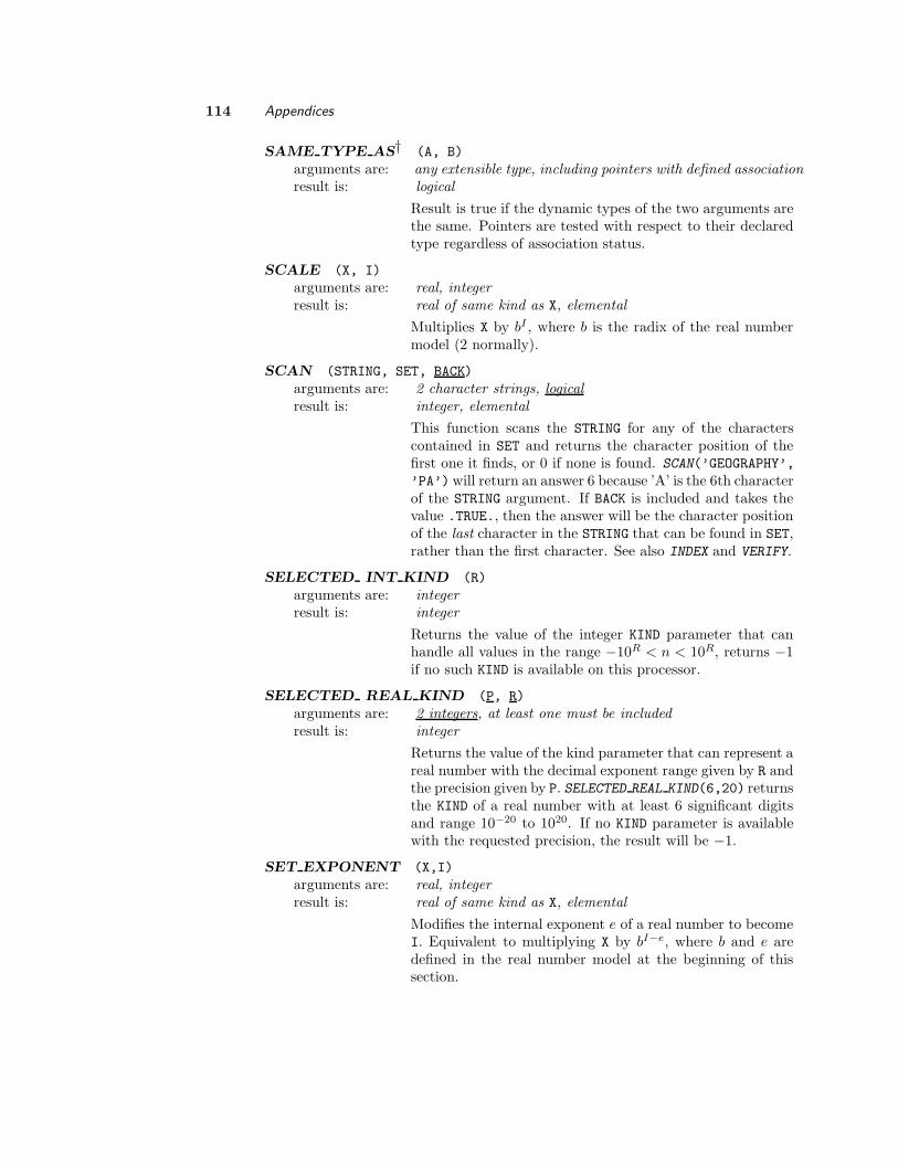
114 Appendices
SAME TYPE AS† (A, B)
arguments are: any extensible type, including pointers with defined associationresult is: logical
Result is true if the dynamic types of the two arguments arethe same. Pointers are tested with respect to their declaredtype regardless of association status.
SCALE (X, I)
arguments are: real, integerresult is: real of same kind as X, elemental
Multiplies X by bI , where b is the radix of the real numbermodel (2 normally).
SCAN (STRING, SET, BACK)
arguments are: 2 character strings, logicalresult is: integer, elemental
This function scans the STRING for any of the characterscontained in SET and returns the character position of thefirst one it finds, or 0 if none is found. SCAN(’GEOGRAPHY’,’PA’)will return an answer 6 because ’A’ is the 6th characterof the STRING argument. If BACK is included and takes thevalue .TRUE., then the answer will be the character positionof the last character in the STRING that can be found in SET,rather than the first character. See also INDEX and VERIFY.
SELECTED INT KIND (R)
arguments are: integerresult is: integer
Returns the value of the integer KIND parameter that canhandle all values in the range −10R < n < 10R, returns −1if no such KIND is available on this processor.
SELECTED REAL KIND (P, R)
arguments are: 2 integers, at least one must be includedresult is: integer
Returns the value of the kind parameter that can represent areal number with the decimal exponent range given by R andthe precision given by P. SELECTED REAL KIND(6,20) returnsthe KIND of a real number with at least 6 significant digitsand range 10−20 to 1020. If no KIND parameter is availablewith the requested precision, the result will be −1.
SET EXPONENT (X,I)
arguments are: real, integerresult is: real of same kind as X, elemental
Modifies the internal exponent e of a real number to becomeI. Equivalent to multiplying X by bI−e, where b and e aredefined in the real number model at the beginning of thissection.

A. Fortran Intrinsic Procedures 115
SHAPE (SOURCE)
arguments are: arrayresult is: integer array
Returns the shape (size and dimensions) of the argumentarray. For an array a with dimensions (-2:2,0:10,3), thenSHAPE(a) is (/5,11,3/). (See UBOUND and LBOUND if youwish to find the actual range of subscripts used, see SIZE ifyou just wish to know the total number of elements.)
SIGN (A, B)
arguments are: 2 numericresult is: numeric, elemental
Transfers a sign from the second number to the absolutevalue of the second. SIGN(6.0, -1.0) is −6.0, SIGN(-6.0,-1.0) is also −6.0, but SIGN(-6.0, 1.0) is 6.0.
SIN (X)
arguments are: real or complexresult is: same as X, elemental
Trigonometric sine function, argument in radians. y = sinx
SINH (X)
arguments are: realresult is: real, elemental
Hyperbolic sine function. y = sinhx
SIZE (ARRAY, DIM)
arguments are: array, integerresult is: integer
Returns the number of elements in an array, regardless of in-dex starting point or number of dimensions. If DIM is included,then only the size of the indicated dimension is returned. Foran array declared as a(-2:2,10), SIZE(a) is 50, SIZE(a,DIM=1)is 5.
SPACING (X)
arguments are: realresult is: real, elemental
Returns the absolute spacing of numbers than can be repre-sented near the argument, given the internal representationof the particular real kind of the argument. For example, ifX is 1000.00 and the next highest number than can be repre-sented on the computer is 1000.01, then the spacing is 0.01.See also NEAREST.

116 Appendices
SPREAD (SOURCE, DIM, NCOPIES)
arguments are: array or scalar of any type, 2 scalar integersresult is: array, same type as SOURCE but 1 higher rank
This adds a dimension to an array by making multiple copiesof SOURCE. DIM indicates which dimension of the new array iscreated, and NCOPIES indicates the size of the new dimension.
For example, if A(1:3) = (/1,2,3/) then the function call B
= SPREAD(A,2,4) creates B(1:3,1:4)=
1 1 1 12 2 2 23 3 3 3
. (Note
that because DIM is 2, the resulting matrix has the same valueregardless of the value of index 2.)
B=SPREAD(A,1,4) will create B(1:4,1:3)=
1 2 31 2 31 2 31 2 3
.
SQRT (X)
arguments are: real or complexresult is: same as X, elemental
Calculates the square root of a number. Unless the argumentis COMPLEX, the argument must be positive and the result willbe positive.
SUM (ARRAY, DIM, MASK)
arguments are: numeric array, integer, logical arrayresult is: numeric scalar
Add up the numbers in an array. If a is a two-dimensionalarray of shape (3,4), then SUM(a) is the scalar sum of all 12numbers in a. SUM(a,DIM=2) is a one-dimensional array oflength 3 whose values are the sums along the second indexof a. if MASK is present, it is a logical expression of the sameshape as ARRAY, and only .TRUE. values of the mask areincluded in the sum.
Algebraically, b = SUM(a) calculates
b =
3∑
i=1
4∑
j=1
aij
in which b is a scalar, whereas b = SUM(a,DIM=2) calculates
bi =
4∑
j=1
aij
in which bi is an array of three numbers.

A. Fortran Intrinsic Procedures 117
CALL SYSTEM CLOCK (COUNT, COUNT RATE, COUNT MAX) (subroutine)arguments: 3 scalar integers, at least one must be present, all INTENT(OUT)
This subroutine returns clock information from a real-timesystem clock, if the system has one. COUNT is the number ofclock ticks since the count was last reset to zero. COUNT RATE
is the number of clock ticks this system clock registers eachsecond. COUNT MAX indicates the maximum count a clock willreach before resetting to zero.
On Sun systems as implemented at UD, COUNT RATE is onemillion, indicating that clock “ticks” of a millionth of a sec-ond are being counted by COUNT. The COUNT resets to zerowhen it overflows the standard integer capacity, so COUNT
from this routine can be used for timing to the millionth of asecond over short periods, but it does not replace DATE AND TIME
for producing wall-clock or calendar information.
TAN (X)
arguments are: real or complexresult is: same as X, elemental
Trigonometric tangent function. Argument in radians. y =tanx
TANH (X)
arguments are: realresult is: real, elemental
Hyperbolic tangent function.y = tanhx
TINY (X)
arguments are: realresult is: real
Returns the smallest possible value (magnitude) the com-puter can represent in the type and kind of the argument.
TRANSFER (SOURCE, MOLD, SIZE)
arguments are: any type or rank, any type or rank, integerresult is: type, kind, and rank of MOLD
TRANSFER takes the actual internal representation of SOURCE(i.e., the actual values at the binary level) and reinterpretsthem with the type, kind, rank, and character length (ifapplicable) of MOLD. As a simple example, suppose c is acharacter string of length 4 and j is a default-sized 4-byteinteger, then after j = TRANSFER ( c, 1 ), j will have thevalue (as an integer) of the bit pattern generated by the 4character codes used to represent c. If SIZE is present orMOLD is an array then the output can be an array of eitherthe size of MOLD or of size SIZE.
TRANSPOSE (MATRIX)
arguments are: two-dimensional arrayresult is: two-dimensional array
Calculates the “matrix transpose” of a two-dimensional ar-ray. If a has shape (3,5), then b = TRANSPOSE(a) is a matrixof shape (5,3) in which b(2,4) has the value of a(4,2).

118 Appendices
TRIM (STRING)
arguments are: character stringresult is: character string
Trim the trailing blank characters off of a character string.TRIM(’Hi there ’) produces the string ’Hi there’.
UBOUND (ARRAY, DIM)
arguments are: array, integerresult is: integer array
Returns the values of the upper bounds (highest index rangenumber) for each dimension of the argument. If the DIM ar-gument is present, returns only the value of the upper boundof that dimension. (See also LBOUND.)
UNPACK (VECTOR, MASK, FIELD)
arguments are: rank one array, logical array, array of same type as VECTORresult is: an array of the same size, shape, and type as FIELD
This takes the elements of VECTOR and expands them into alarger array into the positions in which MASK is .TRUE.. Inpositions in which MASK is .FALSE., the elements of FIELDare copied into the output.
VERIFY (STRING, SET, BACK)
arguments are: 2 character strings, logical scalarresult is: integer, elemental
If all the characters in STRING can be found in SET, then theresult is 0. However, if at least one character in STRING isnot in SET, then the position of the first character not foundin SET is the result.
If BACK is present and .TRUE., then the result is the positionof the last character in STRING that is not in SET. For exam-ple VERIFY(’FORTRAN’, ’ANOFR’) is 4, because the T is thecharacter not in ’ANOFR’. VERIFY(’FORTRAN’, ’ANOF’, .TRUE.)
is 5, because the second R is the last character not in ’ANOF’.

Appendix B. ASCII CodesThe codes found in the following table are the first 128 characters in the ASCIIcollating sequence used on most Unix computers. These are the characters andcodes used by the ACHAR and IACHAR functions. Multi-letter codes below representactions or unprintable characters. Code 8 is “backspace”, 10 is “newline”, 13 is“carriage return”, and 32 is the blank space.
Code Char Code Char Code Char Code Char
0 nul 32 sp 64 @ 96 ‘
1 soh 33 ! 65 A 97 a
2 stx 34 " 66 B 98 b
3 etx 35 # 67 C 99 c
4 eot 36 $ 68 D 100 d
5 enq 37 % 69 E 101 e
6 ack 38 & 70 F 102 f
7 bel 39 ’ 71 G 103 g
8 bs 40 ( 72 H 104 h
9 ht 41 ) 73 I 105 i
10 nl 42 * 74 J 106 j
11 vt 43 + 75 K 107 k
12 np 44 , 76 L 108 l
13 cr 45 - 77 M 109 m
14 so 46 . 78 N 110 n
15 si 47 / 79 O 111 o
16 dle 48 0 80 P 112 p
17 dc1 49 1 81 Q 113 q
18 dc2 50 2 82 R 114 r
19 dc3 51 3 83 S 115 s
20 dc4 52 4 84 T 116 t
21 nak 53 5 85 U 117 u
22 syn 54 6 86 V 118 v
23 etb 55 7 87 W 119 w
24 can 56 8 88 X 120 x
25 em 57 9 89 Y 121 y
26 sub 58 : 90 Z 122 z
27 esc 59 ; 91 [ 123 {28 fs 60 < 92 \ 124 |
29 gs 61 = 93 ] 125 }30 rs 62 > 94 ^ 126 ∼31 us 63 ? 95 127 del
119

120 Appendices
Appendix C. Fortran Archeology
I don’t know what the scientific programming language of 20 years from now
will look like, but I know that it will be called Fortran.
— old joke of uncertain origin (more than 20 years old)
Language Evolution
The opening chapter presented a brief history of Fortran development—a his-
tory that now exceeds half a century. The rate of Fortran language development
has not been constant over this time. Development of new features was continual
from inception of the language through the military-standard extensions added to
Fortran 77. Usually, new features were requested by programmers, implemented
as extensions by compiler vendors, and then standardized after they had become
common practice.
Some of the strength and inertia of modern Fortran programming comes from
the fact that a lot of old code is still useful. We may seem to have two Fortran
languages: a modern subset of Fortran 95 in which all new code is written, and
an older dialect of Fortran 77, mostly with some standard extensions. Code in
variants of Fortran 77 dates back to the era when Fortran was at the peak of its
popularity, so a lot of it is out there.
Programmers trained in the old ways who have never had a need to learn the
new syntax may think of modern Fortran as a different language entirely. However,
anyone comfortable with modern Fortran will need very little additional information
to understand older codes, because all of the old features are included in the newer
language, and only a few obsolete features need to be learned. The purpose of this
appendix is to help programmers trained to use modern features in a modern way
deal with the older code they might encounter.
As languages evolve, standards add new features. In order to maintain back-
ward compatibility, they seldom delete old features. Cross-platform portability is
an elusive goal which also consistently adds to the size of a language. For exam-
ple, standards before Fortran 90 required a default REAL and a DOUBLE PRECISION
type that gave more space to the REAL number, but the standard could not specify
how to allocate those bits of information into precision and without getting into
hardware issues down to the level of chip design. Modern Fortran provides a set of
inquiry functions and KIND specifiers that allow a programmer to control the things
that are most important to a numerical programmer: the precision (number of sig-
nificant digits) and range (maximum power of ten) of the numbers being worked
with. Placing this control within Fortran required a few syntax improvements and
about a dozen intrinsic functions. This has allowed a major improvement in the
portability of a program. Of course, all the old syntax of DOUBLE PRECISION and
its related constant forms, specific functions, and format specifiers is still supported
within the language. Thus, the language grows by always adding new features and
seldom being able to delete anything.
Most additional capabilities enter the Fortran standard because of programmer
demand. Features such as INCLUDE statements or access to command line arguments
were widely implemented as extensions by individual vendors before the standards
committee chose a syntax that could be easily implemented by all the vendors.
121

122 Appendices
Fortran before Fortran 90 did not have any functions, formats, or constant-
value specifiers for binary digits (or octal or hexadecimal). (Fortran 77 did not
actually recognize that computers fundamentally used binary arithmetic—a truly
hardware-independent standard.) Many programmers needed to access their com-
puter words on the bit level, so nearly every compiler system had extensions for
this purpose. Fortran 90 developed a series of intrinsic functions, based on existing
extensions but identical to no particular compiler’s extensions, to acknowledge the
nearly universal practice of extending a compiler in that manner. Giving in to ex-
isting practice has also led to the standardization of INCLUDE, pointers, NAMELIST
input, and system clock inquiries. Fortran 2003 adds in command-line argument
access (while recognizing that command-line operating systems are not universal),
bindings to the way data and subroutines are specified in C (which recognizes that
the major operating systems are written in variations on C), and more objected-
oriented capabilities.
Looking backwards along this trend, a 20-year-old Fortran program written by
a good programmer may be a logical, structured, documented program, but it will
seem like the programmer was doing everything the hard way, particularly when
arrays were involved. That seldom causes a problem, because the old syntax still
works, even if it is not written in a modern style.
More problematically, the old program was probably written by a scientist or
engineer to deal with a particular problem, a particular range of inputs, or a partic-
ular dataset, to be run on a particular computer with one compiler available. That
machine and compiler may have been the only processor for which that programmer
ever wrote code. The program’s purpose may have been perceived as a calculation
to be done once, never to be reviewed once it was decided that the output numbers
were correct. “Scientist-grade code” is a disparaging term for a program that put
no importance on style, portability, documentation, readability, or ability to deal
with new data beyond the orginal purpose.
As you work backwards in time, more and more Fortran codes will contain
extensions or hidden assumptions that worked on the processor the program was
written for, but that will not work or will cause errors on different processors. Old
features that were either in Fortran standards or were commonly known extensions,
which have now been replaced with other standard Fortran features, are the easy
ones. If you encounter references to subroutines and functions or keywords that were
never in the Fortran standard, these will at least be obvious problems, and they
will force you to look up things about a particular operating system or compiler.
There can be worse, hidden nasties, such as tricks that relied on six-bit bytes
or knowing too much about the correspondence between certain integer values and
character codes for some no-longer-used collating sequence. At some point going
back into the Fortran 66 era of codes written for particular mainframes made by
companies long out of the business, the utility of porting old code instead of writing
a new version comes to an end.

C. Fortran Archeology 123
Old Fortran
Going back through older versions of Fortran:
1. What modern features do we lose? In the first step, going to pre-
Fortran 90, this is a big set of features.
2. What old features were in common use? Many of the strangest old
features were very lightly used—you do not need to learn them so much as to
be familiar with the concepts so you can look them up. Some old features were
quite problematic and not easily replaced. These will remain in legacy codes
for a long time, and you need to make sure you understand their implications
if they occur within a code you will be using.
3. How do we make an old code compatible with current new code?
There are a few tools that can help. Some short old codes can be converted,
but avoid converting anything big if possible. Usually, only a few deleted
features and nonstandard features must be converted to run a program on a
modern machine. However, a huge increase in the number of intrinsic func-
tions and reinterpretations of old standards can create situations in which an
old standard-conforming program is still standard-conforming but now has a
different interpretation.
Fixed Form Source
In a system inherited from the days of 80-column punched cards, the column po-
sitions of characters affected their interpretation. The fixed-form source style only
uses 72 characters of each line—columns 73–80 could be used for card identification
numbers or just left blank. The columns have particular uses:
1 A C or * in column 1 indicates that this is a comment line. Comments could
only take up complete lines—no “embedded” comment character for starting
a comment to the right of a statement was available. Totally blank lines were
also comments.
2–5 These columns could only contain digits to make a statement label. Since the
early language required many more statement labels than now, allocating a
significant chunk of the line for this purpose was not unreasonable.
6 Any character except 0 (zero) in column 6 indicated that this line continued
a statement from the previous line. Two common styles: number continued
lines with digits (1, 2, . . .), allowing that 0 could be used to number the initial
line of a long continued statement, or use a nonsyntactic character ($ was a
favorite) so that any mistyping that shifted the continuation character out of
column 6 would generate an error message.
7–72 The actual Fortran statement went into this space.
A first impression might be that early programmers spent their time counting
spaces, but these constraints were easy to deal with. Punched cards for Fortran
had lines drawn at the column boundaries, and later screen editors usually had a
Fortran mode, or could be customized to make typing in the wrong place difficult.
An odd characteristic of fixed-form source is that blank spaces were never
significant in Fortran code. One could insert blank spaces anywhere, including

124 Appendices
within keywords and symbolic names, and one was never required to put in a blank
space.
Programs exist to convert fixed-form source into a form that compiles as either
fixed-form or free-form: put all statements into columns 7–72, continue every mul-
tiline statement with an & sign in both column 73 of the line being continued and
in column 6 of the continuation line, put all statement labels in columns 1-5, and
compress all embedded blanks from symbolic names.
What Old Fortran never had:
No Array Arithmetic or Array Section references. Everything was done
to arrays one subscripted element at a time, usually in DO loops. Exception: whole
arrays could be referenced in I/O lists without subscripts. The lack of array sec-
tion references often required some special tricks when passing parts of arrays into
subroutines—discussed below under “Call-by-Address Tricks.” A related lack was
that there was no array constructor syntax (no use of (/ . . . /) to set all the
elements of a small array).
No Elemental Functions. Without elemental functions, you cannot apply SIN,
COS, SQRT, etc., to all elements of an array at once. As with array arithmetic, the
function had to be applied to one element at a time, normally within a DO-loop.
No Array Reduction and Manipulation Functions. Among the most used,
no SUM, MINVAL, MAXVAL, DOT PRODUCT, MINLOC, or MAXLOC.Also, no ALL, COUNT,
ANY, TRANSPOSE, MATMUL, RESHAPE, EOSHIFT, or any other functions that oper-
ated on array arguments.
No Attributes with Declarations. PARAMETER was a separate statement after a
type had been declared; PARAMETER could only be scalar, not array. Arrays had to be
individually dimensioned, no blanket DIMENSION attribute. No INTENT or OPTIONAL
attributes for dummy arguments. No :: separating attributes from variables in
declarations, because there were no attributes to separate.
Simpler END statements . No END PROGRAM program name or similar END SUB-
ROUTINE or END FUNCTION statements, just plain END.
No MODULEs. No subroutine argument checking at compile time at all!
No SUBROUTINE interfaces, which follows from no MODULEs. With no inter-
face checking between a SUBROUTINE and its callers, there could be no OPTIONAL
arguments, no assumed-shape arrays with (:) dimensions, no use of SIZE, SHAPE,
UBOUND, or LBOUND to find things out about an array passed into a subroutine, no
generic subroutines and functions because there was no INTERFACE.
Missing Control Structures. No unlimited DO, SELECT CASE, WHERE blocks,
EXIT, CYCLE, or FORALL. All of these are easily emulated with GO TO, IF, and DO
structures, albeit with more statement labels and a generally messier syntax.
KIND parameters were less standard. REAL and DOUBLE PRECISION have al-
ways been there, and have always been variable from processor to processor, depend-
ing on storage allocated and the “number model” used to define them. Fortran 90
provided a way to demand a degree of precision that would translate across compil-
ers and processors. Related to these KIND parameters are the inquiry functions that
were missing before Fortran 90: DIGITS, EPSILON, EXPONENT, HUGE, KIND, NEAREST,

C. Fortran Archeology 125
PRECISION, PRECISION, RADIX, RANGE, RRSPACING, SCALE, SELECTED INT KIND, SE-
LECTED REAL KIND, SET EXPONENT, SPACING, and TINY.
Many fewer intrinsic functions. Besides all the intrinsic functions not used
or needed because of the lack of MODULE and KIND information or array arithmetic
there were no standard bit manipulation functions, random number generators,
clock and calendar routines, and signficantly fewer character string manipulation
functions. The bit manipulation functions were often available as extensions, but
these extensions varied greatly.
Old logical operators. The logical operators ==, /=, >, <, >=, and <= were
common extensions in the 1980s, but they were not standard. Comparison operators
were .EQ., .NE., .GT., .LT., .GE., and .LE. instead.
No dynamic allocation. No ALLOCATE, DEALLOCATE. All space requests had to
be known at compile time, which led to major use of special, system-dependent
subroutine calls to accomplish this purpose.
Other advanced features. Derived types and pointers were also missing.
Basic Linear Algebra Subprograms. Look up BLAS for a long list of widely
used routines, implemented in many libraries and compilers, to overcome the lack
of array arithmetic. These were never standard, but were extensively used in old
codes, so the chances of encountering them in old codes are high.
Things that were about the same.
The syntax that stayed the same actually accounts for the majority of the working
code needed to make things happen.
Intrinsic Types. REAL, INTEGER, LOGICAL, COMPLEX, and CHARACTER meant
the same as they do now. DOUBLE PRECISION was a longer precision REAL, but
without the KIND parameters and related functions, it was impossible to tell how
much precision was actually available. Constants were nearly the same: use of
the double quotation mark for character was not standard, and KIND designators
constructed by adding 4 or 8 to a constant were not yet allowed. (Commonly used
type declarators REAL*8 and REAL*4 were never actually standard.)
Control structures: Counted DO and END DO, IF-THEN-ELSE IF-ELSE-END IF
blocks, the single-statement IF, DO WHILE, GO TO, CALL, RETURN, and STOP all
worked the same as now.
IMPLICIT NONE was available, but many people did not use it—familiariarity
with the implicit types was necessary.
Arithmetic has always used the same operators and order of operations, albeit
only with scalars or single array elements in the old Fortran.
Input/Output and FORMAT controls were mostly the same. Fortran 90 formal-
ized edit descriptors for binary, octal, and hexadecimal integers, but these had been
widely available as extensions.

126 Appendices
Commonly used, useful things that have been replaced:
COMMON blocks. See discussion below under “Deprecated Features.”
DATA statements. This is an old form of data initialization, made as a separate
statement from the type declaration. As a simple example, the modern statement
REAL, DIMENSION(4) :: A=(/6.5E3, 25.0, -33.6, 1.38E-226 /)
would require the old set of statements:
REAL A(4)...
DATA A /6.5E3, 25.0, -33.6, 1.38E-226 /
Standard Fortran 77
The previous discussion is about Fortran 77 plus the U.S. Military Standard
extensions that became nearly universal in the 1980s, even though they were not
part of an ISO standard. Strict Fortran 77 loses a few more things. This level
of standardization was common through the early 1980s and was enforced much
longer for some large modeling projects seeking widest possible portability.
No END DO. DO termination required a statement label, but multiple DO statements
could terminate on a single statement. The CONTINUE statement was the preferred
statement for a labeled DO termination, but any statement can be labeled for DO
termination. The obsolescent shared DO termination is discussed below.
No DO WHILE. This construct never was popular anyway.
No IMPLICIT NONE. Workarounds were available for those who did not approve
of implicit typing, but they fell short of strong typing. See the IMPLICIT statement
under Deprecated Features.
No Mixed Case. All code outside character strings must be in a single case.
Nearly everyone thinks that it had to be uppercase, but in fact the standard did
not have a concept of case. Before Fortran 90, standards documents and early
compilers only used uppercase. Fortran arose and propagated on machines that
used six-bit bytes, leading to a 64 character collating sequence that only had space
for one version of each letter. Because support for lowercase itself was an exception,
a few compilers allowed uppercase and lowercase but enforced case dependence, a
la Unix, but that was rare and unpopular. Fortran 95 still did not require lowercase
to be supported, so a standard-conforming compiler may still require all uppercase.
Fortran 2003 requires lowercase support, but it maintains the practice that the cases
are equivalent and interchangeable outside of character constants.
Symbolic names limited to 6 characters. The original IBM 704 computer was
a 36 bit processor using 6 bit bytes. This made it easy for the original Fortran
computer to handle names only up to six characters. That limit persisted in the
standard for 35 years. Many compilers had longer limits, but usually 8 or 17,
seldom as long as the Fortran 95 limit of 31 characters, let alone the Fortran 2003
limit of 63 characters. A pernicious variation: longer variable names were allowed,
but not all characters were “significant.” For example, if a 17 character name is
legal but only the first 8 characters are significant, then RADIATIONUP is the same

C. Fortran Archeology 127
as RADIATIONDOWN as far as the compiler is concerned, because both start with
RADIATIO—pure evil for debugging.
No embedded comments. Only an entire line could be declared as a comment,
with either C or * in column 1. Use of ! to start a comment anywhere on the line,
possibly after a statement, was not allowed.
Standard Fortran 66
Compared to Fortran 77, we lose only a little, but it has quite an effect on the
appearance of the code.
No Block IF. No THEN, ELSE IF, ELSE, END IF, only the single statement IF.
This loss alone makes for the greatest change in appearance of older codes—each
significant decision structure requires a profusion of statement labels and GO TO
statements. Any common modern IF-block of the form
IF (a > 0.0) THEN
b = a ** 1.514
ELSE
b = 0.0
END IF
would turn into something like
IF(A.LE.0.)GOTO11
B=A**1.514
GOTO12
11 B=0.0
12 ( first statement after former block IF)
Some visual complexity arises because a statement label merely indicates that this
line is a potential target. It gives no clue about what type of statement is pointing
at this line (DO termination or one of several kinds of GO TO), nor whether this line
will be reached from before or after the statement, nor whether the label is used at
all. If there were a “nested” set of IF blocks around this in a modern code, you can
be certain that all of them would terminate on the statement labeled 12, so there
is more than one statement pointing at this target. The complete lack of indenting
and spacing in this last example reflects common style (or lack thereof) from the
punched-card era, so expect no help from indented blocks.
No CHARACTER data type. Characters were stored as integer codes, usually
using the INTEGER data type (See discussion of Hollerith data under deleted fea-
tures.) No related concatenation operator or intrinsic functions could be defined
since there was no type. Conversion of a numeric value to its character-string rep-
resentation via READ or WRITE on internal files was not available, but a common
extension involved the use of keywords ENCODE and DECODE for this purpose.
No Standard and Generic Functions. Every function had a special version for
each type. I.e., instead of SIN(X) providing a REAL result for REAL X and a DOUBLE
PRECISION result for DOUBLE PRECISION X, you had to choose SIN or DSIN. All
the usual calculator functions had Dxxx versions. (MIN and MAX were truly weird:
DMIN1, AMIN1, AMIN0, MIN1, MIN0, and a corresponding list of MAX functions.)
Before Fortran 77, intrinsic functions were not formally standardized. All
old compilers had a list of intrinsic functions available, typically including the basic

128 Appendices
“calculator” functions. One name convention was that the Fortran library of func-
tions all ended in F, so there were SINF, COSF, and ABSF functions instead of SIN,
COS, and ABS. These might have come with the constraint that no user-defined
name could be four characters or longer and ending in F, and no user-defined name
could be the same as the intrinsic library name without the F. (I.e., if COSF is an
intrinsic function, then the user cannot define COS for any other purpose.)
Nonstandard intrinsic functions may require finding someone who worked on
the original machine or has access to an old manual—email and Usenet groups can
be quite helpful.
No OPEN. Various operating system methods were used to attach a new unit
number to a file. Older Fortran programs were often incompletely described by their
Fortran code. A control “batch file,” “exec,” or “script” would contain significant
information about the attached files. Knowing the job control or batch control
commands of the operating system may be essential to understanding these. Data
file attachment information may have been entirely offline, or punch-card data may
have been associated with a program by virtue of being stored in the same box.
OPEN became a necessity only when file storage hardware became more variable
and widespread. Early on, the only conceivable I/O devices were large physical
objects: the card reader, the line printer, the card puncher, and some tape drives.
On a given system these would commonly be preconnected to Fortran unit numbers
(from which we have the legacy of preconnected units 5 and 6), and there was
no use for any unit numbers beyond these few. If unit 4 was a tape drive, then
reading from unit 4 required that a tape was present on that drive. Requesting
that a particular tape be mounted on that drive might be done with special system-
dependent subroutine calls, it might involve separate job-control language outside
the scope of the Fortran program, or it might be accomplished with a handwritten
paper form submitted with the card deck. When disk storage facilities existed, some
were only accessible via local library subroutines rather than via the standard READ
and WRITE procedures now used.
Some compilers (notably from Control Data Corporation) required parentheses
and arguments on the PROGRAM statement to define the unit numbers that would be
accessed. For example,
PROGRAM HEAT ( INPUT, OUTPUT, TAPE5=INPUT, TAPE6=OUTPUT )
might have been required to set up the standard input and output connections on
such a machine.
Confronting Old Codes
If you must use old Fortran codes, whether whole programs or subroutines, the
first thing to remember is that you may not need to do anything special. The few
features that were actually deleted from the language have not been widely used
for many years, and many Fortran 95 compilers still support the deleted features
anyway. Trying the old code with a new compiler is always the first step.
Old codes are almost inevitably in fixed-form source, and compilers need all
code within a file to be of one source form or the other. Unix compilers often assume
that a file type of .f implies fixed source form and .f90, .f95, or f03 implies free source
form, but these assumptions can be overridden with command line options. Object
(.o) files created by the compiler are the same whether the source form was free

C. Fortran Archeology 129
or fixed, so codes of two different source forms can always be merged during the
linking step after compiling.
When an old program does not compile or run with an up-to-date (Fortran 95
or Fortran 2003) compiler, likely problems include: use of deleted features, use of
extensions or intrinsic procedures that were never standard, or assumptions were
made about the underlying hardware or initialization. The first two categories
are at least likely to be found and flagged by the compiler. Nonstandard intrinsic
procedures are a common source of questions to Usenet groups, and a number of
old manuals have been put on the Web by computer history buffs. Knowing the
brand of computer on which the program originally ran can be very helpful when
finding old intrinsic procedures.
Hidden assumptions are harder to find and fix. Two hidden assumptions were
common. If a processor had default initialization, every numeric variable was ini-
tialized (usually to zero) at the beginning of a run (this may have been requested by
an option on the compiler or loader). Also, many old programs essentially assumed
the SAVE attribute for all local variables and common blocks in subroutines and
functions because the system had no means of recovering and reusing such storage
space. Some compilers can flag use of uninitialized variables and static storage for
local variables.
Old Features from Old Fortran
Back in the Old Fortran era, a number of now thoroughly strange, somewhat incom-
prehensible features were used. I put them into three groups. Deleted features
were once part of Fortran but have been specifically deleted—they are no longer
part of Fortran. Obsolescent features were specifically designated as such by the
Fortran standards—these are still part of the Fortran language but should never
be used for new code. Designating a feature as obsolescent is a way of warning
programmers that this feature may be deleted in a future standard. Deprecated
features are features that are commonly disliked for new code. Most of these have
been disparaged by other writers, but some may just be against my personal taste.
Deprecation is not a category from the Fortran standards; I think my list follows
widespread opinions among progressive programmers, but it is still just my list.
Deleted Features
All of the following features were deleted from the language in Fortran 95, not
before. All of these should work correctly in a Fortran 90 compiler but must be
removed from programs to work with newer compilers.
Hollerith Data and nH edit descriptor. Before
CHARACTER data were invented for Fortran 77, character strings were held in
numeric REAL or INTEGER variables. (INTEGER was used more commonly than REAL.)
For example, if one needed to write a 40-character label on a machine with 4-byte
(32-bit) integers, then one could declare an array that stores a total of 40-bytes:
DIMENSION LABEL(10)
(Since this dates back to Fortran 66 and earlier, it has been declared using an
implicit type of INTEGER because the name starts with L—the only variables ever

130 Appendices
declared were arrays, since they required a DIMENSION.) To write this out or read
it as a character string required the A format:
READ (5,1000) LABEL
WRITE (6,1000) LABEL
1000 FORMAT (10A4)
If the same I/O statements had been executed with 10I4 instead of 10A4, the integer
equivalent codes would have been written.
Character strings stored this way normally had a number of characters that
was an exact mutiple of the number of bytes in a computer word. Thus, the pre-
vious example has 4 8-bit bytes per word. Bytes were not always eight bits, and
numbers of bytes in a word were not always powers of two. Programmers often
become very familiar with the character codes on their particular machines, and
they could manipulate the value of character string by doing integer arithmetic on
its Hollerith representation. Converting or interpreting such a code may be impos-
sible without obtaining both the collating sequence table for the original machine
and a description of the bit-format used to store numbers in its computer words.
Hollerith data became obsolete with the beginning of Fortran 77, so code has not
been written this way in a long time.
The nH edit descriptor predates the ability to embed character strings between
two apostrophe’s. To write a line with a label, you could write
WRITE (6,1000) A
1000 FORMAT (7HAREA IS,1X,F7.2)
to get output of
AREA IS 1804.28
where the 7H means that the next 7 characters should be put out literally. This
construct was highly susceptible to error, in that if one miscounted the 7 characters,
the format might not be legal, or it might be quite different. Strings expressed in
this way could only be expressed in the old Fortran character set: one case and a
limited set of special characters.
Early extension: when nH edit descriptors were still the norm and apostrophe
delimiters had not been developed, some compilers used a nonstandard * delimiter:
1000 FORMAT (*AREA IS*,1X,F7.2)
NonInteger Do Index Variables were allowed in Fortran 77 but not neces-
sarily in earlier versions. They were widely regarded as a mistake, and were seldom
used. If you find one of these, conversion to an integer DO variable is required. One
good reason for getting rid of these is that the number of passes through a loop is
unpredictable, leading to codes that could have very different results on different
machines. If a DO block begins with DO A=0.0,10.0 with A as a REAL variable, a
quick glance would indicate that the loop will pass 11 times, with the last pass oc-
curring at A=10.0, but the loop might pass only 10 times if on the last pass A comes
out with a value slightly larger than 10, such as 10.000001, which could happen
with the imprecision of REAL arithmetic.

C. Fortran Archeology 131
Branching to an END IF from outside the IF block. This is a minor
reinterpretation of the older standards. In the following example, the first GO TO
is legal and the second is not. To get rid of the problem,you need to remove the
10 from the END IF and add a 10 CONTINUE statement just after the END IF as a
target for the GO TOs.
IF (. . .) THEN...
GO TO 10...
10 END IF...
GO TO 10
PAUSE statement. The PAUSE statement was designed to bring a program to
a halt temporarily, requiring some operator intervention before a program would
resume. There was no way to standardize what actions should take place to cause
a program to resume without getting into operating system issues, so it was a non-
portable statement. In command-line interfaces where a program is being invoked
from a terminal or X window, PAUSE can be replaced with a read from the keyboard
with no input list: READ (*,*)
ASSIGN statement, assigned GO TO and assigned FORMAT. These features
allowed assigning a statement label to a variable name, so later that variable name
could be the target of a GO TO or format identifier.
ASSIGN 10 TO K...
GO TO K
When K is used this way, it must be an integer scalar, and it must not be used for
anything else. Usage of these was rare. Getting rid of them directly (via simple
editing, without reanalyziing the code) might best involve the SELECT CASE con-
struct. Firstly, replace each ASSIGN 10 TO K statement with K = 10. Then, the
GO TO statement can be replaced with
SELECT CASE (K)
CASE(10)
GO TO 10
CASE(20)
GO TO 20
. . . more cases as neededEND SELECT
The SELECT CASE structure is also useful for removing the computed GO TO or the
alternate RETURN, as discussed below.
A more justifiable use for ASSIGN was the need to provide alternate format
references to an I/O statement in versions of Fortran that predated the CHARACTER
type. As an example
ASSIGN 1000 TO K...
WRITE (6,K) io list

132 Appendices
This was occasionally needed in Fortran 66 and earlier because of the lack of
CHARACTER data and manipulation methods. Replacing such a structure (again
directly, without reanalyzing the code) can be done by defining a sufficiently long
character variable, setting that variable equal to the format string at each ASSIGN
statement, and then using the character variable name as the format identifier.
CHARACTER(LEN=40) :: FString ! use whatever length needed...
FString = ’format 1000 edit descriptors’ ! replaces ASSIGN...
WRITE (6,FString) io list ! replaces WRITE statement
Obsolescent Features
The features discussed in this section were declared obsolescent officially in the
Fortran 95 standard. Standards committees understand that legacy code is a sig-
nificant strength of Fortran, so deletion of features that will cause legacy code to
be noncompliant with current compilers is done slowly and carefully. Thus, obso-
lescent features are like a posted warning: these features are still a supported part
of any Fortran 95 compiler, but they may be deleted in future standards, so do not
use them for new code. No features will be deleted from Fortran without them first
spending some years on the obsolete list, during which public feedback about these
proposed deletions will influence the standards committee. All of the Fortran 95
deleted features listed above were declared obsolete in Fortran 90. Declaring a
feature obsolete does not mean it will be deleted in the next round. Most of the
obsolescent features below were also declared obsolescent in Fortran 90, but For-
tran 95 did not delete them, nor did Fortran 2003, implying that these ancient ways
of doing things remain sufficiently embedded in working code that compiler writers
must accommodate them.
Computed GOTO. The shotgun control structure, it looks like this:
GO TO (10, 20, 40, 50) K
where K is an integer (or an integer expression). If K is 1, 2, 3, or 4, then the
statement will go to statements labeled 10, 20, 40, or 50, respectively. If K is less
than 1 or greater than the number of labels given in parentheses, there is no jump,
and the program continues with the statement after the computed GO TO. IF blocks
or the SELECT CASE construct can easily replace this with more readable code.
Arithmetic IF. Before logical expressions existed, branch control was based on
evaluation of a numeric arithmetic statement, tested against zero. As an example
IF (B) 20, 50, 10
If the numeric variable B was less than zero, control would jump to statement 20, if
B was equal to zero, control would jump to statement 50, and if B was greater than
zero, control would jump to statement 10. The same statement label could appear
more than once, and the numeric variable could be replaced by an expression. Thus:
IF (A - C) 10, 10, 20

C. Fortran Archeology 133
says that if A is greater than C then go to 20, and if A is less than or equal to C,
then go to 10. Usually, a direct replacement of arithmetic IF with logical IF blocks
is easy and obvious.
A never-standard variation that came later is the two-branch logical IF:
IF (A.GT.C) 10, 20
evaluates the logical expression in parenthesis (is A greater than C?), and transfers
to the first statement label (10) if the expression is true, and the second (20) if
the expression is false. Part of the silliness of this construct is that it essentially
requires a statement label of 10 or 20 on the subsequent statement, without which
it would not be executable unless it had third statement label to be jumped to from
somewhere else—uber spaghetti code.
Old-Style DO terminations. We use DO and END DO as block constructors.
Other DO styles include use of a statement label to identify which termination goes
with DO statement, as in
DO 20 J=N,M...
20 CONTINUE
These forms are not considered obsolescent, but I consider them deprecated. Use
named looped labels for DO loops that need labels and otherwise don’t clutter up the
code with numbers. What is considered obsolescent is the shared DO termination:
DO 20 I=1,N
DO 20 J=I+1,N...
20 CONTINUE
and another obsolescent form is the DO termination on a statement other than
END DO or CONTINUE:
DO 10 I=1,N
10 A(I) = B(I)
An example of both obsolescent constructs combined:
DO 30 I=1,N
DO 30 J=I+1,N
30 A(I,J) = B(J,I)
Only shared DO termination and the termination on an executable statement other
than END DO or CONTINUE are considered obsolescent by the standard, but I do not
recommend the use of anything other than DO-END DO, with name labels where
needed.

134 Appendices
Alternate RETURN. This was an attempt to deal with error exits from subroutines.
Alternate returns are indicated by CALL statement with things like *100 in the actual
argument list or a subroutine with * in the dummy argument list. For example, if
you see a call statement like
CALL GOOFY ( MICKEY, DONALD, *100, *200)
then your corresponding SUBROUTINE will have * placeholders in the argument list:
SUBROUTINE GOOFY ( MINNIE, DAISY, *, * )
and the subroutine will have an integer expression attached to the RETURN statement:
RETURN integer expression
If the integer expression has the value of 1 or 2, then after returning to the CALL
statement, control will jump directly to statements labeled 100 or 200, respectively,
in this example. If integer expression is less than 1 or greater than the number
of alternate return codes provided, or if a RETURN statement is reached that has
no integer expression, then execution proceeds with the statement after the CALL
statement as usual.
The alternate return mechanism can better be replaced by returning an addi-
tional dummy argument as an error code or return code (often, the same value as
the integer expression), and testing the value of that return code immediately after
the CALL statement, either in an IF block or in a SELECT CASE construct.
Fixed-Form Source. Fixed-form source is considered obsolescent—don’t write
any new code that way.
Data statements in executable. DATA statements should be considered depre-
cated compared to newer initialization syntax. However, allowing them to be mixed
in among the executable statements instead of strictly with the declaration state-
ments created the illusion that they were truly executable instead of being one-time
initializations.
Statement Functions. It was allowed to define a single-statement function at
the beginning of a subroutine or program, just after the declarations and just before
the executables. Example:
ES(T)=611.2*EXP(17.67*T/(243.5+T))
can be included as a single line at the beginning of a subroutine or program. Then
later on within that same program, ES(T) is available as a function. Recommended
replacement is to use a CONTAINS statement and create an internal procedure.
CHARACTER*n declarations. CHARACTER*10 is equivalent to CHARACTER(LEN=10)
or CHARACTER(10). Use one of the latter two.
Assumed-Length Character Functions. Seldom used, declared obsolescent as
a way of cleaning up an inconsistency.

C. Fortran Archeology 135
Deprecated Features
The features in this section have no special mention in the Fortran standards. They
are widely considered to be too heavily embedded in the legacy code, in ways that
are not easily removed by automated editing programs, for deletion anytime soon.
Hence, they are not on the obsolescent list because they cannot reasonably be moved
to the deleted list. However, they are bad ways of doing business for new code.
COMMON blocks. Before modules were invented, checking that dummy arguments
and actual arguments matched in type, kind, rank, and intent, and making sure
that they occurred in the same order between CALL and SUBROUTINE statements
was a major source of aggravation and error. A way around this was to put all
the major data arrays, and perhaps scalars, into COMMON blocks. Imagine that this
statement occurred in the declaration section of a program:
COMMON /NODES/ X(100,3), U(100,3), T(100), TR(100)
This declares four arrays (inevitably implicitly typed as REAL) with the dimensions
shown, and allows them to be used within this program. If the same COMMON state-
ment appears in another subroutine, then these same arrays are available in that
subroutine, even though they are not in the argument list, and even if that sub-
routine is not called directly by the program. That is, COMMON blocks allow data to
be shared among subroutines, programs, and functions, independently of argument
lists and calling trees. A source of flexibility and error is that COMMON variables can
be redimensioned or renamed between subroutines. If another subroutine declares
COMMON /NODES/ X(300), V(100,3), T(50), T2(150)
then that subroutine has access to the same 800 numbers as the previous one.
However, X in this subroutine is a one-dimensional array of length 300 instead of a
two-dimensional (100,3) array, U has the same dimension and shape but has been
renamed as V within this subroutine, T in this subroutine is the first half of T from
the other routine, and the last half of T has been combined with TR to form the
array T2.
There can be many COMMON blocks in a program, uniquely identified by the
name enclosed in slashes (NODES in this example). At most one COMMON block can
be “blank” common, with no name (and no slashes, just COMMON variable list).
COMMON blocks are a rampant source of errors that result from renaming and
resizing arrays. It became preferred practice that a COMMON block declaration used
exactly the same names and dimensions in every case, often by pulling them in via
INCLUDE statements (which were a common extension until Fortran 90 standardized
them) so that no differences could arise via typing mistakes. New code uses the data
sections of MODULES for this purpose.
Another problem was that a COMMON block made data available in a subrou-
tine that were not needed by that subroutine. An egregious use of COMMON would
be to declare all variables in a common block and INCLUDE that block in every
routine, effectively making every variable available everywhere. Using our NODES
example: a subroutine that only needed access to X and TR would have the entire
COMMON /NODES/ block, and a later programmer would have no way of knowing
that the other two arrays were not needed, used, or changed in the routine. With
MODULE data, the ONLY clause of a USE statement can restrict access and declare
which arrays are actually used in the current routine.

136 Appendices
BLOCK DATA subprograms. BLOCK DATA introduces a scoping unit whose only
purpose is to declare COMMON blocks and initalize them via DATA statements. Only
one BLOCK DATA subprogram can exist in a program, so this is the only scoping unit
that has no name. New code uses data MODULEs instead.
EQUIVALENCE statements. The fugu banquet of Fortran: dangerous, inter-
esting, occasionally useful (in the old days). EQUIVALENCE establishes a storage
association between Fortran variables, so that they occupy the same locations in
computer memory.
DIMENSION X(100), U(100)
EQUIVALENCE (X,U)
After these declarations, X and U occupy the same space in computer memory. The
presumption is that an array is needed where the context makes it logical to call it
X—perhaps it is coordinates. In another part of the program, when X is no longer
needed and its information can be discarded, it may be useful to call the same space
U—perhaps it is speed. In other words, we reclaim the space used by X and use it
as U. It is up to the programmer to ensure that there is no overlap in time where U
starts being filled while information in X is still needed.
Another creative use of EQUIVALENCE:
DIMENSION VEL(100,3), U(100), V(100), W(100)
EQUIVALENCE (VEL(1,1),U(1)), (VEL(1,2),V(1)), (VEL(1,3),W(1))
After this declaration, we can put our velocity vectors into a single two-dimensional
array VEL, or we can refer to the individual vector components as U, V, and W.
EQUIVALENCE did not need to work on entire array names.
What each EQUIVALENCE pair ties together are two storage locations, not two
values. Hence, variables of different types can be tied together. This does not mean
that the array will have the same values in two different types. Suppose we declare
INTEGER IWORK(1000)
REAL WORK(1000)
EQUIVALENCE (IWORK,WORK)
and then execute
WORK(1) = 10.0
WRITE (6,’(I10)’) IWORK(1)
The output will not be 10, but rather will be the integer whose internal (bit-by-bit)
representation is the same as a REAL 10.0—a result that can only be understood in
consideration of how the computer represents data internally.
The names in this last example hint at the only justifiable use I ever found for
EQUIVALENCE. Before the existence of ALLOCATABLE arrays, scratch space for things
like sorting routines, equation solvers, or interpolation functions had to be calcu-
latable by the compiler and allocated at the beginning of a program run. Different
library routines might need different amounts of scratch space at different times,
but one could easily guarantee that on exit from a routine, the information in the
scratch space array was no longer needed. Work arrays needed for various indepen-
dent routines and could be tied together with EQUIVALENCE. Dynamic allocation
eliminates the need for this old trick.
Call-by-Address tricks with external subroutines. Every programmer of Old
Fortran became very familiar with the storage sequence used for arrays. When

C. Fortran Archeology 137
an array was being passed into a subroutine, the only piece of information actually
going into the subroutine was the address of the first element of the array—nothing
about type, number of dimensions, size, or actual index in calling program.
Suppose you had the common circumstance of having a two-dimensional array
that needed to be operated on by a subroutine one column at a time. In Fortran 90,
the solution might look like this:
REAL, DIMENSION(nr,nc) :: a...
DO c=1,nc
CALL Crunch ( a(1:nr,c) )
END DO
in which case CRUNCH will receive a one-dimensional array of length nr, and it can
determine that size from the SIZE intrinsic function if needed, as in
SUBROUTINE Crunch ( a )
IMPLICIT NONE
REAL, INTENT(INOUT) :: a(:)
INTEGER :: n...
n = SIZE(a)
In Old Fortran, array sections were not allowed, the colon was not used as a
deferred-shape indicator, intent attributes did not exist, and the size of an array
had to be explicitly passed into the subroutine as an integer argument. Also, the
column of a two-dimensional array was passed into the subroutine by indicating
only the first element of the column.
REAL A(NR,NC)...
DO 10 J=1,NC
CALL CRUNCH2 ( A(1,J), NR )
10 CONTINUE
and the corresponding subroutine could start with:
SUBROUTINE CRUNCH2 ( A, N )
INTEGER N
REAL A(N)
The important part of this example is that A(1,J) in the actual argument list points
to the first element of each column, in sequence, as the loop goes through the range
of NC.
The storage-sequence consideration is trickier if we wish to pluck out a row at
at time of the array. In modern Fortran, the appropriate block is
DO r=1,nr
CALL Crunch ( a(r,1:nc) )
END DO
and no modification to the subroutine is required. In Old Fortran, if we simply
change the call to CALL CRUNCH2 ( A(J,1), NC ) then we will be pointing at the
correct starting point, but the numbers needed by CRUNCH2 are not adjacent. The
requirements for this situation are:

138 Appendices
REAL A(NR,NC)...
DO 10 J=1,NR
CALL CRUNCH3 ( A(J,1), NC, NR )
10 CONTINUE
and the corresponding subroutine would be:
SUBROUTINE CRUNCH3 ( a, n, inc )
INTEGER N, INC
REAL A(*)...
DO K=1,N*INC,INC
A(K) = . . .
where INC (for increment), is used in the subroutine as “stride” variable—in other
words the size of the first dimension in the calling program is just the distance
between adjacent elements as far as the subroutine is concerned. Similar but less
capable than the (:) of modern Fortran, a dummy argument array of size (*) is
only allowed in the last dimension of an array.
If a subroutine needed to make use of a two-dimensional array, Old Fortran
had another set of potential problems. Consider the common data analysis problem
of taking a set of input data and calculating a correlation matrix. The dataset
might look like X(NOBS,NVARS), where NVARS is the number of different variables
and NOBS is the number of observations (such as locations or times) for each vari-
able, and the correlation matrix would then be a square two-dimensional matrix
CORR(NVARS,NVARS). It would be very common to write a program with these ar-
rays dimensioned for the largest problem anticipated, say
REAL X(2000,10), CORR(10,10)
and then find the actual values of NVARS and NOBS on reading the dataset (and
checking to make sure they are within the size limits in the dimensions). Suppose
we have read a dataset X and have found a value for NOBS that is less than 2000 and
a value for NVARS that is less than 10.
Now we call a correlation subroutine:
CALL Correlate ( X(1:NOBS,1:NVARS), CORR(1:NVARS,1:NVARS) )
and this could successfully call a subroutine with the following declarations:
SUBROUTINE Correlate ( X, CORR )
IMPLICIT NONE
REAL, INTENT(IN) :: X(:,:)
REAL, INTENT(OUT) :: CORR(:,:)
INTEGER :: nv, no...
nv = SIZE(X,DIM=2)
no = SIZE(X,DIM=1)...
In Old Fortran, besides needing to pass in the sizes of the arrays, a calling program
typically needs to pass in the leading dimensions of the arrays as dimensioned in
the calling program, such as:

C. Fortran Archeology 139
CALL CORREL ( X, NVARS, NOBS, CORR, 2000, 10 )
for a subroutine:
SUBROUTINE CORREL ( X, NV, NO, CORR, LDX, LDC )
INTEGER NV, NO, LDX, LDC
REAL X(LDX,NV), CORR(LDC,NV)
C Only X(1:NO,1:NV) CORR(1:NV,1:NV) will be used.
A two-dimensional array in the subroutine must have the first dimension be the
same as it was where the space was allocated, because an unfilled first dimension
leads to gaps in the storage sequence. An unfilled last dimension is of no concern,
since the extra elements are all past the end of the used elements. To illustrate this,
look at an array dimensioned (4,3) of which only (2,2) needs to be passed into a
subroutine:Storage Declared Passed
Sequence (4,3) In?
1 (1,1) Yes
2 (2,1) Yes
3 (3,1) No
4 (4,1) No
5 (1,2) Yes
6 (2,2) Yes
7 (3,2) No
8 (4,2) No
9 (1,3) No
10 (2,3) No
11 (3,3) No
12 (4,3) No
Professionally written libraries, such as IMSL and NAG, used “leading dimen-
sion” variables exhaustively when they have two-dimensional arrays as arguments.
Locally written or scientist-written programs may be less likely to use them because
a code may be more problem specific, dimensioned exactly to the size needed. Also,
when one is designing a program top to bottom, often the order of dimensions can
be chosen to avoid such problems. For example, consider a climate data set with 12
months of data for a large N of stations. If a program needs to analyze something
about the entire seasonal cycle for each station, then dimensioning the data array
as (12,N) puts the monthly data for a particular location in adjacent storage loca-
tions. If a program needs to map out monthly fields, then dimensioning the data
array as (N,12) allows the entire spatial dataset for a particular month to occupy
adjacent storage locations. Algorithm and intention drive the data structure.
Modern Fortran provides two improvements that remove the need for “leading
dimension” variables and for considerations of algorithm when designing the data
structure. Firstly, the array passing information (in module subroutines) sends a
complete characterization of the array or array section, not just the address of the
first element. Secondly, ALLOCATABLE arrays and automatic arrays make it possible
to generate a larger fraction of arrays at exactly the right size, allocating them at
run time after the needed size has been determined.
However, here is one area where speed issues can force one back to thinking
about storage sequences. All Fortran compilers in actual existence still allocate

140 Appendices
arrays in the first-index-first order, because old Fortran is a subset of Fortran 90 and
old programs depended on this order. Many (most?) computers rely on processing
systems in which a small amount of memory (the cache) is accessed at a much
faster rate than the main memory of the computer. The processor achieves its best
speed only when all the data it needs are on the cache. Thus, in large arrays, best
processing speed happens when most of the DO-loops or array operations go through
nearly adjacent elements, which often means designing a code so that innermost DO-
loops or array operations move across the first index as much as possible.
Alternate ENTRY. A subroutine or function can be started in multiple locations
with this statement. Consider:
SUBROUTINE NAME1 ( dummy argument list 1 )
Declarations section...
some executable code...
ENTRY NAME2 ( dummy argument list 2 )...
more executable code...
RETURN
END
If a calling program issues CALL NAME1 with an argument list corresponding to
the first dummy argument list, the whole subroutine will be executed. Execution
control will pass through the ENTRY statement as if it were a CONTINUE. If a calling
program issues CALL NAME2, then the part of the subroutine before ENTRY NAME2
will be skipped. Almost always, this would be better done by having NAME2 be a
separate subroutine that could be called from NAME1 as well as from other places.
Implicit typing and IMPLICIT statements. The implicit type rules of Fortran
are: if a variable starts with I through N, it has type INTEGER, otherwise it is REAL.
We use IMPLICIT NONE everywhere to void those implicit type rules and force the
compiler to check for declared type on all variables. This is the way things are
done now, and some of us think that the standards body missed an opportunity
when they did not attach “strong typing” (the opposite of implicit typing) to the
free-form source code so that we could stop putting IMPLICIT NONE everywhere and
just assume it. (Only the fixed-form source code style requires implicit typing for
backwards compatibility.)
However, when implicit typing is your paradigm, you make it general and
flexible. An IMPLICIT statement could be used to customize implicit typing so that
a programmer would never need to actually declare any variable’s type. Consider
IMPLICIT DOUBLE PRECISION (A-H,O-Z)
This was just a modification of the standard implicit typing so that all the default
REAL variables would be default DOUBLE PRECISION instead. (Many compilers had,
and still have, compiler flags to accomplish autodoubling for this same purpose.)
IMPLICIT COMPLEX (W,Z)

C. Fortran Archeology 141
This forces any variable name starting with W or Z to be of type COMPLEX. In the
implicit typing paradigm, a programmer would rather declare an implicit starting
letter or two for complex variables, instead of declaring each complex variable ex-
plicitly, so that a variable in the program starting with W or Z would be instantly
recognizable as complex. The implicit typing paradigm went along with many-page
programs that were not broken up by subroutines, so forcing a reader to look all
the way to the top of a program just to find out the type of a variable was rude:
use implicit types and the types become obvious.
IMPLICIT rarely was used to break up the standard Fortran implicit typing
for REAL and INTEGER, just to add implicit letters for types other than REAL and
INTEGER, as shown here. Once the dangers of implicit typing were widely recognized,
but the IMPLICIT NONE extension was not yet universal, a kludge was common:
IMPLICIT LOGICAL (A-Z)
or
IMPLICIT CHARACTER (A-Z)
When you see one of these, most likely the programmer was trying to get the
benefits of IMPLICIT NONE on a compiler that didn’t support that extension. A
mistyped variable name for an intended REAL or INTEGER variable is highly likely
to produce an error message if the misspelled variable is assumed by the compiler
to be a nonnumeric type.
It may come as a pleasant surprise to folks who have never seen any IMPLICIT
statement except IMPLICIT NONE that this latter statement was not derived from
scratch by someone with a strange sense of English word order, but rather is ex-
tended from the earlier IMPLICIT statement in a reasonably logical manner.
Missing “Prettyprinting”, short variable names. “Prettyprinting” is an old
term for using blank spaces and blank lines to improve the readability of codes.
Nowadays, we indent control structures (good editors do it for us automatically);
put blank spaces between the word elements of a Fortran statement; establish case
conventions for keywords, variables, and scoping unit names; and separate control
blocks with blank lines. Older codes often have no indentation, no blank spaces,
and an obsession with putting a C at the beginning of every blank line.
Fortran was designed to be a language based on algebraic analogies, so it is
natural to use X for coordinates, U and V for speeds, or T for temperatures. You might
find short old codes where the only multiple-character variable names are spelled-out
greek letters, like RHO and ALPHA. The assumption with this kind of programming
is that the Fortran variable names are a direct translation of a technical report or
paper that is expressed in traditional algebraic forms. There is absolutely nothing
wrong with these short variable names when a close relationship exists between a
Fortran program and a technical report or text that explains the program.
However, many old programs used short, nonmnemonic variable names out
of laziness, perhaps desiring to minimize time spent with the coding form and
keypunch machine (admittedly, a reasonable desire). X and Y are reasonable, but
when you find various dimensions as N, NN, NNN, and MM (with no mnemonic sense),
or see III and JJ as DO-indexes, you have encountered lazy variable naming.
Modern fashion has been to use longer variable names that describe the quan-
tity, so that the Fortran program can be read independently of its background

142 Appendices
technical report. For example, the strain rate tensor ǫij old style might have been
EPSDOT(I,J), but now is more likely to be called strain rate(i,j). This is a good
thing, up to a point. SUNTEMP or TSUN are better than Temperature of the Sun,
because at some point in variable length, verbosity becomes a problem, not a clari-
fier. We still need comment lines in the declarations section to explain our variable
names, so variable names should not be turned into comment-length descriptions.
(Subroutine names might reasonably be longer. Subroutines may be called in to-
tally separate files and libraries from their descriptions, so a descriptive subroutine
name is worthwhile, and it won’t clog up an arithmetic expression.)
Excessive lengthening of variable names can arise from object-oriented pro-
gramming, in which variables are not variables, they are subobjects of some greater
object class that happen to have the ability to store information. In Fortran, we
see the beginnings of this style with derived types. If you see a name such as
Node%temperature(element%boundary index) with percent signs buried in long
variable names, then you need to learn about user-defined types.
Carriage Control. Back when unit 6 was preconnected to a line printer, the first
character of any output was not for actual printing, but for controlling the printer—
a “carriage control” character. What you will see in old codes is that output to
unit 6 or to any unit that was expected to be printed usually left the first character
blank, but occasionally used another character. The carriage control codes were:
1 Eject a new page before printing this line.
0 Go down two lines before printing this line (double space).
(Blank space.) Normal single spacing—go down one line and print.
+ Go down zero lines before printing (over printing).
Any other characters in column one had an undefined effect, some systems just
stripped anything else off and treated it as a blank. These carriage-control char-
acters are sufficiently embedded into Fortran codes that many printing commands,
such as the Unix lpr command and enscript, can still recognize them and obey
them if proper flags are invoked. Fortran no longer supports these, but they are
not nonstandard either. They are just outside the standard.
In new codes, we don’t use these. Normal single-spacing happens by default,
and we get double-spacing by putting a slash at the beginning of a format, or
occasionally by a blank WRITE statement. The ADVANCE=NO clause in a WRITE state-
ment can produce overprinting, and ACHAR(12) is the ASCII page-eject character,
Control-L.
External Procedures. Already discussed herein is the lack of the MODULE scoping
unit in Old Fortran, and some of the implications of the lack. What a MODULE
creates for a calling program, among other things, is an explicit interface, which
allows a calling unit, at compile time, to be aware of the dummy argument names,
their sequence, and the intent, type, kind, and rank of each argument. When
you encounter an old library of Fortran subroutines and functions you wish to
use, subroutines will not, typically, be encased in modules, and the compiler will
not be able to determine any of those things during compilation. Matching of all
these characteristics, via sequenced actual arguments, is entirely the problem of the
programmer.
The external procedures introduced in Chapter 13 should be considered depre-
cated features in the context of writing them for new code, but they are included in
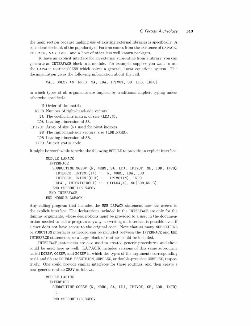
C. Fortran Archeology 143
the main section because making use of existing external libraries is specifically. A
considerable chunk of the popularity of Fortran comes from the existence of lapack,
fftpack, nag, imsl, and a host of other less well known packages.
To have an explicit interface for an external subroutine from a library, you can
generate an INTERFACE block in a module. For example, suppose you want to use
the lapack routine SGESV which solves a general, linear equations system. The
documentation gives the following information about the call:
CALL SGESV (N, NRHS, SA, LDA, IPIVOT, SB, LDB, INFO)
in which types of all arguments are implied by traditional implicit typing unless
otherwise specified.:
N Order of the matrix.
NRHS Number of right-hand-side vectors
SA The coefficients matrix of size (LDA,N).
LDA Leading dimension of SA.
IPIVOT Array of size (N) used for pivot indexes.
SB The right-hand-side vectors, size (LDB,NRHS).
LDB Leading dimension of SB.
INFO An exit status code.
It might be worthwhile to write the following MODULE to provide an explicit interface.
MODULE LAPACK
INTERFACE
SUBROUTINE SGESV (N, NRHS, SA, LDA, IPIVOT, SB, LDB, INFO)
INTEGER, INTENT(IN) :: N, NRHS, LDA, LDB
INTEGER, INTENT(OUT) :: IPIVOT(N), INFO
REAL, INTENT(INOUT) :: SA(LDA,N), SB(LDB,NRHS)
END SUBROUTINE SGESV
END INTERFACE
END MODULE LAPACK
Any calling program that includes the USE LAPACK statement now has access to
the explicit interface. The declarations included in the INTERFACE are only for the
dummy arguments, whose descriptions must be provided to a user in the documen-
tation needed to call a program anyway, so writing an interface is possible even if
a user does not have access to the original code. Note that as many SUBROUTINE
or FUNCTION interfaces as needed can be included between the INTERFACE and END
INTERFACE statements, so a large block of routines could be included.
INTERFACE statements are also used to created generic procedures, and these
could be used here as well. LAPACK includes versions of this same subroutine
called DGESV, CGESV, and ZGESV in which the types of the arguments corresponding
to SA and SB are DOUBLE PRECISION, COMPLEX, or double-precision COMPLEX, respec-
tively. One could provide similar interfaces for these routines, and then create a
new generic routine GESV as follows.
MODULE LAPACK
INTERFACE
SUBROUTINE SGESV (N, NRHS, SA, LDA, IPIVOT, SB, LDB, INFO)...
END SUBROUTINE SGESV

144 Appendices
SUBROUTINE DGESV (N, NRHS, DA, LDA, IPIVOT, DB, LDB, INFO)...
END SUBROUTINE DGESV
SUBROUTINE CGESV (N, NRHS, CA, LDA, IPIVOT, CB, LDB, INFO)...
END SUBROUTINE CGESV
SUBROUTINE ZGESV (N, NRHS, ZA, LDA, IPIVOT, ZB, LDB, INFO)...
END SUBROUTINE ZGESV
END INTERFACE
INTERFACE GESV
MODULE PROCEDURE SGESV, DGESV, CGESV, ZGESV
END INTERFACE
END MODULE LAPACK
Any program with USE of this module can now use CALL GESV, and so long as the
types of the 3rd and 6th arguments match each other, the compiler will find the
right routine.
With access to the source code, generation of INTERFACE blocks can be done
with freely available software, although such programs can only determine type,
kind, and rank of arguments to the degree that they are declared in the old code, and
they cannot determine INTENT for dummy arguments. A feature of imsl, lapack,
and probably other well-developed libraries is that interfaces have been developed
like that shown above for GESV which also put many of the arguments into OPTIONAL
status if the size of the problem can be inferred from the size of the real arrays. For
example, GESV, shown above, can now be called with just the A and B arguments,
and the rest of the arguments will be either determined from the shape of A and B
or given a default value that can be altered by including another argument.