Embed Size (px)
Citation preview

What are (Computer) Languages?
A useful computer language is:
• ‘easy’ for a human to understand
• ‘easy’ for a compiler to convert to the obscuremachine instructions and OS calls that the computerunderstands – a process called ‘compilation’.
Of course one may argue about what the word ‘easy’ above means.
1

Portability
It should not be necessary to rewrite programs merelybecause one wishes to run them on a different type ofcomputer or on a different operating system.
A mere recompilation should be sufficient.
A language with a well-defined and well-supportedstandard tends to achieve this ideal (e.g. F90, C,Java). A program written in a language without awidely accepted standard (e.g. BASIC) often requires amajor rewrite in order to use it on a different computer.
2

FORmula TRANslation
Fortran is a venerable language designed to translatescientific formulae into a form usable by computers. Itwas not designed as a general-purpose language.
Fortran was originally developed by IBM in the late1950’s. The first official standard was published byANSI in 1966, followed by significant revisions in 1977.The next standard, published in 1990, representeda more dramatic change, and that published in1995 a very minor set of changes. The relevantstandards committee still exists, and further revisionsare expected.
ANSI: American National Standards Institute.
C is also quite an old language. So-called K&R C was developed in Bell Labs in the early1970s, and was launched on the world in 1978, with the first ANSI standard published in 1989,thus creating ANSI C.
3

Fortran Today
Fortran may be nearing fifty years old, but it is far fromdead!
Most large numerical codes are still written in Fortran:examples include most weather forecasting programs,many ‘numerical wind-tunnels’ and most quantummechanical electronic structure codes. Thus themajority of the CPU time of big supercomputers, bothnational supercomputers and those in Cambridge, isspent running Fortran.
Not being a general-purpose language, there are some things Fortran is very bad at. Anyonetrying to write a compiler or operating system in Fortran is probably mad or about to becomemad. However the ‘old’ University Library electronic catalogue, which is soon to be replaced,is written in Fortran, even though this is far from the sort of application for which Fortran wasdesigned.
Fortran’s historic advantage is its simplicity: easy for humans to learn, easy for compilersto translate into the optimal sequence of instructions for a computer to execute. On somemachines (such as vector Crays from the early to mid 1990s), the same algorithm written inFortran and C would typically run ten to twenty times faster when written in Fortran.
4

Hello
$ less hello.f90write(*,*) ’Hello, world.’end$ f95 -o hello hello.f90$ ./helloHello, world.$
First one must create the above two-line program using an editor.
The program consists of statements, one per line. The first writes a message back to thescreen, the second, end, finishes each and every Fortran program.
The UNIX less command shows us the contents of the text file we have created: press ‘q’ toexit.
The UNIX f95 command compiles that file, assuming it is valid Fortran. We have asked itto name the resulting binary program, which we will be able to run, ‘hello’. Omitting ‘-ohello’ would result in the default name of ‘a.out’ being used.
The UNIX command ./hello runs this new program we have just created. The initial ‘./’indicates that this is not a pre-installed system program, but something to be found in ourcurrent directory.
Although print* can be used as a synonym for write(*,*), the more general form will beused throughout these notes.
5

Variables
A variable is simply a label for an area of memoryreserved for storing some data.
integer ii=3write(*,*) ’i is ’,ii=i+iwrite(*,*) ’i is ’,iend
Here we start by choosing to use ‘i’ as the label to refer to an area of memory in which asingle integer value can be stored.
The next line stores the value 3 in this location.
The following line prints out i. Notice that ‘write(*,*)’ happily accepts a comma-separatedlist of things to print out.
The next line appears to be mathematical nonsense, but = should be interpreted as meaningassignment not equality. Thus the line calculates i + i, and stores the answer back into theoriginal location that i occupied. The old value of i is overwritten.
The final two lines should need no explanation.
6

More variables
We may define as many variables as needed. Theirnames can be up to 31 characters long, the first mustbe alphabetic, the others alphanumeric or underscore.
Unlike UNIX, Fortran is not case-sensitive. In a Fortranprogram, ‘small’, ‘SMALL’ and ‘Small’ are consideredequivalent. Inconsistency will confuse humans though.
The operators +,-,*,/ and ** are available, the lastbeing exponentiation.
integer small, smallersmall=3smaller=2write(*,*)small-smaller, small/2small=smallersmaller=smallwrite(*,*)smallerend
This program prints 1 twice, then 2. Note that 3/2 is 1: so far we have met only integers.Also, the two assignments near the end do not swap the contents of small and smaller:indeed, the antepenultimate line is utterly pointless here.
7

Interacting
Examples always appear a little pointless until theyperform something slightly non-trivial. Thus a way ofgetting a program to prompt for input is introduced atthis early stage:
real a,b,c,x,ywrite(*,*) ’Please input coeffs of quadratic’read(*,*) a,b,cx=(sqrt(b*b-4*a*c))/(2*a)y=-b/(2*a)write(*,*)’Roots are ’,y-x,’ and ’,y+xend
real defines a variable to be floating point, rather than integer.
read(*,*) reads a list of values from the keyboard. The values read can be separated byspaces or be on separate lines, but not separated by commas.
b*b-4*a*c is equivalent to (b*b)-(4*a*c), just like normal algebra. It is not (b*b-4)*a*c.
The sqrt function calculates the square root of its argument.
8

Less Variable
Occasionally it is useful to define a variable in such away that it cannot be changed when the program runs.Such a variable is called a parameter, and everythingabout it can be determined when the program iscompiled.
real piparameter (pi=3.141593)
Here pi can be used like any other variable, exceptthat any attempt to change its value will result in anerror.
N.B. All declarations and parameter statements mustprecede the executable lines of a program.
9

Conditional execution
The above program has many deficiencies, one of whichbecomes apparent if it is given the input ‘1 0 1’.
This can be solved by adding the following linesimmediately after the read:
if ((b*b-4*a*c)<0) thenwrite(*,*)’No real roots’stop
endif
The lines between the if and endif are executed onlyif the condition on the if line is true. The stopinstruction will terminate the program.
Humans enjoy seeing parts of the code indented in order to emphasis the structure, as above.
Computers don’t care, and will not check that the indenting is consistent with the meaning.
10

More Conditions
Fortran has the ‘standard’ set of comparison operators:<, <=, ==, >=, > and / = (not equal).
One can also combine the results of comparisons usingthe operators .and., .or. and .neqv. (xor).
if ((a==0).and.(b==0).and.(c==0)) then
might be useful. As might
if (a<0) thenwrite(*,*)’Quadratic has a maximum’
elsewrite(*,*)’Quadratic has a minimum’
endif
The above errs for a = 0.
N.B. = is assignment, == is equality test.
11

More Control
So far all the examples have shown programs executingline by line from the first line to the last, maybe skippingsome lines when if is used. One very useful additionto this model is that of repeated execution: looping.
integer ido i=1,20write(*,*)i,i*i,i**3
enddoend
The code between the do and enddo is executed twenty times, with the variable i being set toeach of the values from 1 to 20 in turn for each iteration of the loop. The output looks like:
1 1 12 4 83 9 274 16 64. .. ..
12

Neatness
The output of the above program does not fall intothe neat columns that one might hope for. This canbe improved by using a format statement to tell thewrite statement precisely what to do.
integer ido i=1,20write(*,10)i,i*i,i**3
enddo10 format(i4,i6,i8)
end
The second * of the write statement has beeen replaced by a 10. This tells the compiler notto guess what layout is required, but rather to look for a format statement somewhere in theprogram and labelled by a 10. This statement then says: one integer, padded to a width offour characters, ditto six, ditto eight.
The format statement may occur before or after the write. Many writes may refer to thesame format statement. The format statement is completely ignored at the point when itwould be due for execution. The label can be any integer of five or fewer digits.
The complete list of options for format is large.
13

Infinite loops
integer i
dowrite(*,*)’How many burgers, sir?’read(*,*)iwrite(*,*)’Have a nice day!’
enddoend
This is bad practice: there ought to be some way ofstopping a program. Adding
if (i==-1) exit
to the loop after the read would achieve this.
exit causes the program to jump to the statement following the current loop, whether theloop is infinite or finite.
14

Factorisation
integer i,p,sqrt_pwrite(*,*)’Input no. to test’read(*,*)psqrt_p=sqrt(real(p))do i=2,sqrt_pif (mod(p,i)==0) thenwrite(*,*)p,’ is divisible by ’,istop
endifenddowrite(*,*)p,’ is prime’end
mod(a,b) calculates the remainder after dividing a by b
As sqrt does not accept integer arguments, the function real, which converts integers toreals, is called first.
The above algorithm is not optimally fast!
15

Faster Factorisation
integer i,p,sqrt_pwrite(*,*)’Input no. to test’read(*,*)p
if (mod(p,2)==0) thenwrite(*,*)p,’ is divisible by 2’stop
endif
sqrt_p=sqrt(real(p))do i=3,sqrt_p,2if (mod(p,i)==0) thenwrite(*,*)p,’ is divisible by ’,istop
endifenddowrite(*,*)p,’ is prime’end
The full syntax of a do statement is do i=start,end,step, where the ‘,step’ is optional. Ifgiven, it specifies how much to add to i between each iteration of the loop. The final iterationwill be the last one which does not cause i to exceed end.
16

The structure of a simple program
• declarations of variables & parameters
• executable statements
• the end statement
Comments (read by humans, ignored by computers)can be added by placing a ‘!’ on a line. Everythingafter the exclamation mark will be ignored by thecompiler.
A long statement can be split across two physical linesby placing a ‘&’ as the last character of the first line:
write(*,*) &’A somewhat wordy greeting to you all’end
17

Terminology
Operator: +, −, ∗, /, ∗∗Constant: data whose value is known at compile timeVariable: data whose value may change during
program executionFunction: sqrt, cos, sin, etc.
Expression: mathematically valid combination of theabove
Argument: expression on which function actsDeclaration: reservation of memory for a variable
Rather informal definitions. As examples:
real a,b,c ! declarationsparameter (c=5.0) ! c is a real constant, as is 5.0
b=sqrt(c) ! c is the argument of the function sqrt! brackets are required around arguments
a=sqrt(0.4*c) ! 0.4 and c are real constants, * is an operator! 0.4*c is a real constant expression (=2.0)
a=a/b ! a/b is a real variable expressiona=a**2 ! 2 is an integer constant, a**2 a real variable expression...
18

Data Types
So far we have seen integers and reals as data types.
Integers have a range of about ±2× 10⁹.
Reals have a range of about ±1.7× 1038 and about 7decimal digits of precision.
However, another type of real exists with a rangeof about ±9 × 10307 and about 14 decimal digits ofprecision. This is far more useful.
There is also a type called complex for dealing withcomplex numbers (stored simply as two reals: real partand imaginary part).
Compilers may offer more than the above two precisionof reals.
The above assumes standard IEEE-754 data types. Almost every computer uses these. ElderlyCrays and IBM mainframes might not, PCs do.
19

Constants
A constant is simply a number occuring directly in theprogram:
i=i+3
i is a variable, and 3 a constant.
The type of a constant is integer, unless it contains adecimal point or an exponent, when it is real.
Exponents can be specified as 1.3E12 meaning 1.3 ×10¹².
Using a D rather than an E for the exponent causesthe constant to be double precision, that is, enjoy thelarger of the above ranges. Hence 5E50 is (probably)an error, whereas 5D50 is fine.
20

What’s your kind?
One can enquire about the kind of a real number, anddefine another variable to be of a suitable precision:
integer r12parameter (r12=selected_real_kind(12))real (r12) :: x,y
The integer parameter r12 is given the value the the compiler uses to distinguish its sort ofreal that has at least 12 decimal digits of precision. The variables x and y are declared to beone of these. The double colons are required to separate the variables declared from the listthings modifying the real.
integer dpparameter (dp=kind(1d0))real (dp) :: x,y
In a similar fashion, here x and y are each declared to be of the same kind of real as 1d0, i.e.double precision.
N.B. I did not invent this syntax.
21

The Difference
integer ix,iy,dpreal rx,ryparameter(dp=kind(1.0d0))real (dp) :: dx,dy
ix=5 ; rx=5 ; dx=5iy=3 ; ry=3 ; dy=3
write(*,*)ix/iywrite(*,*)rx/rywrite(*,*)dx/dyend
The output from compiling and running the above is:
11.66666661.6666666666666667
A semicolon can separate statements, just as using separate lines does.
22

Complex
The complex type is fully supported, and all thestandard functions can take complex arguments andreturn complex values. It has different kinds in thesame way that real does.
integer dpparameter(dp=kind(1.0d0))complex ccomplex (dp) :: dc
c=-2 ; dc=-2c=sqrt(c) ; dc=sqrt(dc)
write(*,*)cwrite(*,*)dcwrite(*,*)dc-cend
Other functions supporting the complex type include: sin, cos, tan, asin, acos, atan,log, exp and others.
23

Conversions
Conversions between different types and kinds occurautomatically at the last possible moment.
integer i,jreal a,b,ci=2 ; j=3
a=i ! a is 2.0b=i/j ! b is 0.0c=real(i)/j ! c is 0.66.....
The operators +, -, * and / all convert their operands to the same type and kind beforecarrying out the operation. The type and kind of the answer is the type and kind of theconverted operands. The conversion always involves promotion, i.e. movement to the right inthe sequence integer, real, complex and also in the sequence single precision, double precision.
An assignment will convert the type and kind of the right hand side to that of the leftimmediately before the assignment is done. Promotion or demotion may occur.
Most built-in functions (sqrt, trig functions) return the same type and kind as their argument,and do not accept integer arguments.
24

Vagueness
You may discover that programs compile happilyeven if none of the variables used are declared.Simply referencing a variable causes it to be declaredautomatically.
This is bad.
Firstly the type may not be what you expect: integerif the first letter of the variable is in the range i-n, realotherwise.
Secondly, some common mistakes cannot be spottedautomatically:
real salary, taxsalary=15000tax=(salary-4000)*0.23salery=salary-taxwrite(*,*) salaryend
25

Being precise
This unhelpful default behaviour can be suppressed bythe use of the statement implicit none. This turnsoff the implicit declarations which caused referencingthe misspelt ‘salery’ above not to be an error.
implicit nonereal salary, taxsalary=15000tax=(salary-4000)*0.23salery=salary-taxwrite(*,*) salaryend
Attempts to compile this example will fail.
implicit none must precede any declarations.
26

Arrays
Simple scalar variables do not cover every need inPhysics. Thus there exist arrays: variables containingmultiple scalars.
One dimensional arrays, or vectors, are used as follows:
real position(2)
position(1)=-0.02position(2)=52.2
and thus the two element one dimensional variableposition stores our latitude and longitude. Similarly
integer marks(150)
could store the marks of a whole class.
27

More dimensions
real v1(3),v2(3),mat(3,3)...do i=1,3v2(i)=0do j=1,3v2(i)=v2(i)+v1(j)*mat(i,j)
enddoenddo
A simple form of matrix-vector multiplication.
Fortran permits up to seven dimensions.
28

Array terminology
integer i,jreal x, mat(100,100)
defines x to be a (scalar) variable and mat to be a twodimensional array.
mat(i,j) is an element of the array, and i and j arethe array indices or subscripts.
Indices must be integers or integer expressions. mat(2*i,j+7) is quite valid.
The bounds of the array are (1-100,1-100) and anyindices must lie within this range.
Exceeding the bounds of an array is a common error, and is often referred to as ‘falling off theend’ of the array. A reference to mat(101,100) would be such a mistake. The program willnot necessarily stop at this point. . .
An array element can be used anywhere that a scalar variable is valid.
29

Memory
Clearly real mat(3,3) must take nine times as muchmemory as simply real x. Indeed, the matrix will belaid out in memory simply as mat(1,1), mat(2,1),mat(3,1), mat(1,2), mat(2,2) ...mat(3,3).
Thus if mat(i,j) is suddenly requested, the computerknows where mat(1,1) is stored, and adds an offsetof (i-1)+3*(j-1) to find mat(i,j).
Beware! real space(1000,1000,1000) looksinnocent, until one realises that it will require 4GBof memory (assuming 4 bytes per real).
The indices usually start at one, but this can bespecified:
integer map(-20:20,-20:20)
is a 1681 element two-dimensional array whose indicesrange between ±20.
30

Dynamic Arrays
The arrays shown so far are called static, because theirsize is specified at compile time. They cannot grow orshrink.
Dynamically allocated arrays can respond to precisestorage needs at run time.
integer msizeinteger, allocatable :: map(:,:)
read(*,*) msize
allocate(map(-msize:msize,-msize:msize))...deallocate(map)
This will be similar to the previous snippet if 20 is input.
The program will stop with an error if an allocate fails (e.g. not enough memory).
Notice the use of the colon as a placeholder for the as yet unknown dimension sizes in thedeclaration. The keyword ‘allocatable’ defines this to be a dynamic array.
The end statement will automatically deallocate any remaining arrays, though one may do soexplicitly anywhere after the last point at which each array is used.
31
Implicit loops
An array element is just like any other variable, so oneway of copying one array to another would be:
do i=1,na(i)=b(i)
enddo
Fortran90 provides an abbreviated syntax for this:
a=b
Similarly
a=b*c
sets a(i)=b(i)*c(i) for the whole array.
This syntax requires a, b and c to be the same length, or for b and/or c to be simple scalarvariables or constants (e.g. a=2*a doubles all the elements of a).
There is no magic here: the execution time will be as long as if the loop were written explicitly.
32

Array Functions
Fortran90 also provides some functions which actdirectly on arrays. These include:
sum(a)∑
a(i)product(a)
∏a(i)
dot product(a,b)∑
a(i)b(i)maxval(a) value of largest element
maxloc(a) indices of largest element
matmul(a,b) vector or matrix product
and minval and minloc too.
maxval and minval work on multidimensional arrays, and hence maxloc and minloc returna one dimensional integer array giving the list of indices corresponding to the location. E.g.
integer a(3,3),i(2)a=1 ; a(2,3)=2i=maxloc(a)
sets i(1)=2 and i(2)=3.
matmul returns a vector or matrix, and one argument should be a matrix, the other avector or matrix of suitable shape that the multiplication is mathematically reasonable. Notethat c=a*b performs element-wise multiplication, cij = aijbij , whereas c=matmul(a,b)
performs standard matrix multiplication cij =P
aikbkj .
33

Eratosthenes
integer i,j,imax,prime_maxinteger, allocatable :: primes(:)
write(*,*)’Input largest number for search’read(*,*)prime_maxallocate(primes(prime_max))primes=1 ! Sets all elements of array to 1imax=sqrt(real(prime_max))
do i=2,imaxdo j=2*i,prime_max,iprimes(j)=0
enddoenddo
do i=2,prime_maxif (primes(i)==1) write(*,*)i
enddoend
Note the use of a non-unit stride in the loop over j: j takes the values 2*i, 3*i, 4*i. . .
Note the shortened form of the if statement: the then is replaced by a single statement toexecute if the condition is true, and there can be no else section.
34
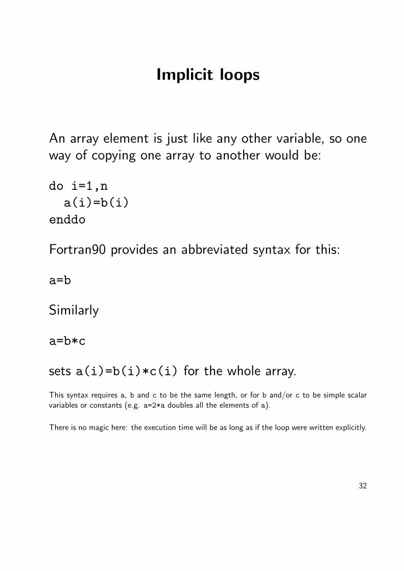
Random Answers
integer i,trials,hitsreal x,y
trials=1000000 ; hits=0
do i=1,trialscall random_number(x)call random_number(y)x=2*x-1 ; y=2*y-1if ((x*x+y*y)<1.0) hits=hits+1
enddo
write(*,*)’pi is approx ’,(4.0*hits)/trialsend
This program calculates π by calculating the area of the unit circle by testing points at randomin the ±1 square.
The built-in subroutine random number sets its argument to a random value in the range0 ≤ x < 1. If passed an array, it sets all the elements to different random values.
This program will give a different answer each time it is run: try it!
35

Decisions
integer diereal x
call random_number(x)die=1+6*x
select case (die)case (1:3)write(*,*)’Stay in bed’
case (4,5)write(*,*)’Skip lecture’
case (6)write(*,*)’Accuse linguist of laziness’
case default ! This should never happenwrite(*,*)’Attend lecture’
end selectend
Although the above is possible using if . . . else if . . . else if . . . else . . . endif, theabove construction can look tidier. In the case statement, (a:b) specifies a range, (a,b) twodiscrete values, and default what will happen if none of the case conditions matches.
A more practical use of the above would be controlling the motion of a particle performing arandom walk.
36

Factorials
No set of programming examples is complete withoutthis:
integer i,n,dpparameter (dp=kind(1.0d0))real (dp) :: fact
write(*,*)’Please input n’read(*,*)n
fact=1do i=2,nfact=fact*i
enddo
write(*,*)n,’ factorial is ’,factend
The double precision real is used for its greater range than integer or real.
37

Extending Fortran
module fact_modcontainsfunction factorial(n)integer i,nreal (kind(1.0d0)) :: factorialfactorial=1do i=2,nfactorial=factorial*i
enddoend function
end module
program testuse fact_modinteger iwrite(*,*)’Please input i’read(*,*) iwrite(*,*)i,’ factorial is ’,factorial(i)
end
38

The Details
The program now starts with a module which containsone function definition.
The function definition is reasonably straightforward.Notice that here the function is going to return a realvalue of kind that of 1.0d0, so the function nameis declared as though it were a variable of that typeand kind, and the value assigned to that variable whenthe function ends is the value which the function willreturn to the calling program. The type of the functionarguments must also be declared.
The unnecessary but clarifying program statementmarks the start of our program. It immediately specifiesthat it wishes to use the module just declared, andthen it calls factorial just as it would any otherFORTRAN function.
Note that the module precedes the program in the source file, and that the module name isnot the same as any variable or function name.
factorial, as defined here, takes an integer argument and returns a real. A function neednot return the same type as its argument(s).
39

The Broader Picture
Variables declared within a function are independentfrom any declared elsewhere. In the above example iis used for different purposes in the main program andthe function.
Thus two different people can write the main programand the function, and, provided they agree on whatarguments the function takes, and on what it returns,neither need know anything about the internal detailsof the other’s code.
This makes managing largish programs with multipleprogrammers possible!
40
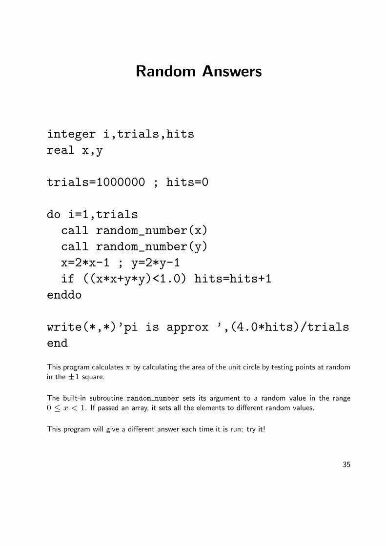
Subroutines
A subroutine is very like a function. Consider swap.f90:
module swap_modcontainssubroutine swap(i,j)integer i,j,tmptmp=i ; i=j ; j=tmp
end subroutineend module
program swapituse swap_modinteger small,smallersmall=3 ; smaller=2write(*,*) small,smallercall swap(small,smaller)write(*,*) small,smaller
end
41

Subroutines in more detail
A subroutine returns no value itself, and has to be calledexplicitly with a call statement. It can, however, alterits arguments.
So can a function, but it is considered very bad practice.
How are the arguments modified? When the abovesubroutine was called, it was not passed ‘3’ and ‘2’directly, but rather the addresses in memory of ‘small’and ‘smaller’.
Simply the addresses. Not their names.
The subroutine read from these addresses, assuming itwould find integers stored there. And then it wroteback to those addresses. When the main programcontinued, the values stored in the memory locationsit calls ‘small’ and ‘smaller’ had thus changed.
Arguments are passed to functions in the same way.
42

Libraries: the Refuge of the Lazy?
Laziness in programming can be a virtue. Rewritingan algorithm that someone else has already writtenis pointless (unless one does it better). People sellcollections of well-written functions and subroutines inbundles called libraries.
We have already used libraries implicitly, for thestandard Fortran library includes definitions of the trigfunctions amongst other things.
To use extra libraries we must include something inour program to tell the first phase of the compilationprocess to expect to find that something has been leftundefined, and then we must tell the final phase, thelinker, where to find it.
For the NAG library we are to use, this is quitestraightforward.
The NAG library, developed by the Oxford-based Numerical Algorithms Group, is copyrightedcommercial software. The version we shall use was developed for FORTRAN77, so does notmake use of all the features of F90. Most noticeably, its routine names suffer from a sevencharacter limit, rather than a 31 character limit.
43

Very simple NAG
First a test just to show successfully compiling andrunning a program calling NAG.
use nag_f77_a_chapterwrite(*,*)’Calling NAG identification routine’write(*,*)call a00aafend
which should be compiled with
f95 nag_test.f90 -lnag
The output produced by this program is:
Calling NAG identification routine
*** Start of NAG Library implementation details ***
Implementation title: Linux (Intel) NAGWare f95 (RedHat 6.x)Precision: double
Product Code: FLLUX19D9Mark: 19A
*** End of NAG Library implementation details ***
44
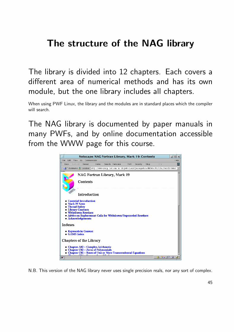
The structure of the NAG library
The library is divided into 12 chapters. Each covers adifferent area of numerical methods and has its ownmodule, but the one library includes all chapters.
When using PWF Linux, the library and the modules are in standard places which the compilerwill search.
The NAG library is documented by paper manuals inmany PWFs, and by online documentation accessiblefrom the WWW page for this course.
N.B. This version of the NAG library never uses single precision reals, nor any sort of complex.
45

A non-trivial NAG example: matrixdeterminant
A quick scan of the documentation produces theslightly cryptic:
1 PurposeF03AAF calculates the determinant of a real matrixusing an LU factorization with partial pivoting.
2 SpecificationSUBROUTINE F03AAF(A, IA, N, DET, WKSPCE,
IFAIL)INTEGER IA, N, IFAILreal A(IA,*), DET, WKSPCE(*)
3 DescriptionThis routine calculates the determinant of A using theLU factorization with partial pivoting, PA = LU, whereP is a permutation matrix, L is lower triangular and Uis unit upper triangular. The determinant of A is theproduct of the diagonal elements of L with the correctsign determined by the row interchanges.
46
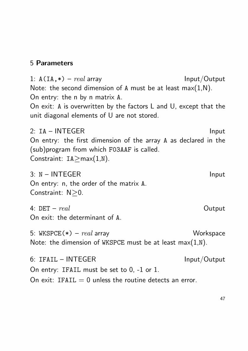
5 Parameters
1: A(IA,*) – real array Input/Output
Note: the second dimension of A must be at least max(1,N).
On entry: the n by n matrix A.On exit: A is overwritten by the factors L and U, except that the
unit diagonal elements of U are not stored.
2: IA – INTEGER Input
On entry: the first dimension of the array A as declared in the
(sub)program from which F03AAF is called.
Constraint: IA≥max(1,N).
3: N – INTEGER Input
On entry: n, the order of the matrix A.Constraint: N≥0.
4: DET – real Output
On exit: the determinant of A.
5: WKSPCE(*) – real array Workspace
Note: the dimension of WKSPCE must be at least max(1,N).
6: IFAIL – INTEGER Input/Output
On entry: IFAIL must be set to 0, -1 or 1.
On exit: IFAIL = 0 unless the routine detects an error.
47

Interpretation
One would expect a subroutine which calculates adeterminant to need arguments including the array inwhich the matrix is stored, the size of the matrix, anda variable into which to place the answer. Here thereare just a couple extra.
Because the library is written in F77, which doesnot support dynamic memory allocation, it is oftennecessary to pass ‘workspace’ to a routine. This spacethe routine will use for its own internal temporaryrequirements. Hence WKSPCE(*).
Because F77 has no decent definition of what ‘singleprecision’ and ‘double precision’ mean, all reals aredescribed as real. In this version, this meansreal (kind(1.0d0)).
Finally, array dimensions of unknown size are denotedby a ‘*’, not a ‘:’ – another F77ism.
48

An example
use nag_f77_f_chapterreal (kind(1.0d0)) :: m(3,3),d,wrk(2)integer i,n,ifail
m(1,1)=2 ; m(1,2)=0m(2,1)=0 ; m(2,2)=2
i=3 ; n=2 ; ifail=0
call f03aaf(m,i,n,d,wrk,ifail)
write(*,*)’Determinant is ’,dend
49

Notes on F03AAF example
First the relevant NAG module is included, so that thecompiler can do some checking of arguments to thesubroutine.
Try swapping the m and i on the call to f03aaf and recompiling.
The array which will hold the matrix, the subroutine’sworkspace and the output variable are all declared.The arrays could have been dynamic if we so chose.
The variables are initialised. The matrix is simply twicethe identity.
The routine is called, and the result written out. Noticethat the 2x2 matrix is held in a 3x3 array, so the arraysize and the matrix size differ. This was done on awhim.
The full NAG documentation offers example programstoo, albeit in F77.
Try finding the determinants of:„1 23 4
«and
„1 −1−1 1
«
50
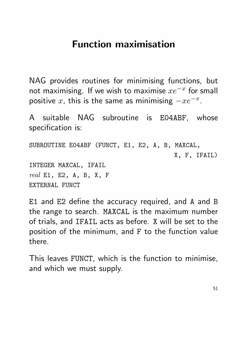
Function maximisation
NAG provides routines for minimising functions, butnot maximising. If we wish to maximise xe−x for smallpositive x, this is the same as minimising −xe−x.
A suitable NAG subroutine is E04ABF, whosespecification is:
SUBROUTINE E04ABF (FUNCT, E1, E2, A, B, MAXCAL,
X, F, IFAIL)
INTEGER MAXCAL, IFAIL
real E1, E2, A, B, X, F
EXTERNAL FUNCT
E1 and E2 define the accuracy required, and A and Bthe range to search. MAXCAL is the maximum numberof trials, and IFAIL acts as before. X will be set to theposition of the minimum, and F to the function valuethere.
This leaves FUNCT, which is the function to minimise,and which we must supply.
51

Passing subroutines to subroutines
The NAG documentation for this reads:
1: FUNCT – SUBROUTINE, supplied by user External Procedure
This routine must be supplied by the user to calculate the value
of the function F (x) at any point x in [a, b]. It should be
tested separately before being used in conjunction with E04ABF.
Its specification is:
SUBROUTINE FUNCT(XC, FC)real XC,FC
1: XC – real Input
On entry: the point at which the value of F is required.
2: FC – real Output
On exit: FC must be set to the value of the function F at the
current point x.
FUNCT must be declared as EXTERNAL in the (sub)program from
which E04ABF is called. Parameters denoted as Input must not
be changed by this procedure.
52

Writing for NAG
So NAG is asking us to supply a subroutine (not afunction) which takes two arguments, and returns thevalue of the function it is evaluating in the second.
The references to EXTERNAL refer to the old F77 style offunction and subroutine declarations: we can continueto use modules as before.
Of course this example is trivial analytically, the resultbeing a minimum of −1/e at x = 1. However, itis good to start with examples whose results one cancheck!
53

Function minimisation: E04ABF
module x_ex_modcontainssubroutine x_ex(x,f)real (kind(1.0d0))::x,ff=-x*exp(-x)
end subroutineend module
program minimizeuse nag_f77_e_chapteruse x_ex_modinteger ifail,maxitreal (kind(1.0d0))::e1,e2,a,b,x,f
e1=0; e2=0 ! Routine will use defaultsa=0.5 ; b=1.5 ; maxit=50 ; ifail=-1
call e04abf(x_ex,e1,e2,a,b,maxit,x,f,ifail)
if (ifail==0) thenwrite(*,*)’Minimum of ’,f,’ at ’,x
elsewrite(*,*)’Minimum not found ’,ifail
endifend
54

Variables in modules
Sometimes it is useful to have variables (or constants)declared once and used in different functions andsubroutines. One example would be:
module constantsreal (kind(1.0d0)), parameter :: &
pi=3.141592653589793d0, &h=6.62606891d-34
end module
module print_pi_modcontainssubroutine print_piuse constantswrite(*,*)’pi is ’,pi
end subroutineend module
program hbaruse constantsuse print_pi_modwrite(*,*)’hbar is ’,h/(2*pi)call print_pi
end
55

Integration
Numerical integration, often called quadrature, is acommon task: analytic integration can quickly becomeimpossible!
As an example we shall consider a situation wherethe analytic result is (relatively) easy, and where thenumerical approach is hard as the range of integrationis infinite. However, NAG can cope with this.
The integral to consider is:
∫ ∞
−∞e−λx2
dx
So that this can readily be evaluated for differentparameters λ, we shall pass λ via a module.
The NAG routine we shall use is D01AMF.
56

module lambda_modreal (kind(1.0d0)) :: lambda
end module
module gauss_modcontainsfunction gaussian(x)use lambda_modreal (kind(1.0d0)) :: gaussian, xgaussian=exp(-lambda*x**2)
end functionend module
program integrateuse lambda_mod ; use gauss_moduse nag_f77_d_chapterinteger, parameter :: lw=1000, liw=lw/4integer i, inf, ifail, iwrk(liw)real (kind(1.0d0)) :: b, result, err, epsabs, &
epsrel, wrk(lw)inf=2 ; ifail=1epsabs=-1 ; epsrel=1d-8
do i=1,20lambda=0.1d0*icall d01amf(gaussian,b,inf,epsabs,epsrel, &
result,err,wrk,lw,iwrk,liw,ifail)write(*,*) lambda,result
end doend
57

File I/O
Writing directly to a file is convenient when the outputis too much to fit on the screen! This can be achievedthus:
integer iopen(20,file=’cubes.dat’)do i=1,100write(20,10)i,i*i,i**3
enddoclose(20)
10 format(i6,i8,i10)end
The open statement creates a file called ‘cubes.dat’ and associates it with I/O unit number20. This statement must come before the first use of that unit number in a write statement.
The first * in the write statement is now revealed to be the unit number. The close is goodpractice, and should follow the last use of that I/O unit. The end statement should also closeany units still open. More details are given at the end of these notes.
58

When it all goes wrong
Programs inevitably have bugs, arising from a varietyof causes.
• Syntax of F90 misunderstood
• Details of library call misunderstood
• Brain forgot what it did a few lines back
• Fingers improvised
It is therefore essential to test programs thoroughly ondata for which the correct results are known: not allbugs cause instant crashes!
59
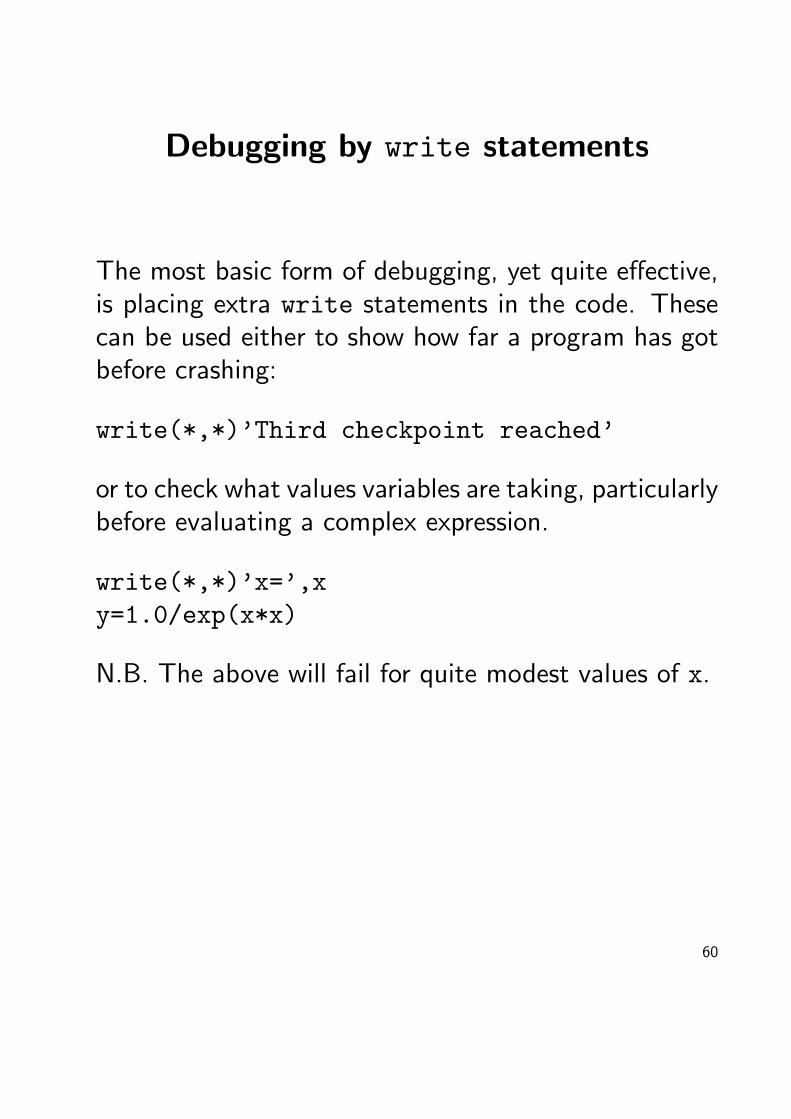
Debugging by write statements
The most basic form of debugging, yet quite effective,is placing extra write statements in the code. Thesecan be used either to show how far a program has gotbefore crashing:
write(*,*)’Third checkpoint reached’
or to check what values variables are taking, particularlybefore evaluating a complex expression.
write(*,*)’x=’,xy=1.0/exp(x*x)
N.B. The above will fail for quite modest values of x.
60

Run-time checks
real x(2,10)integer ido i=1,1000x(1,i)=ix(2,i)=i*i
enddo...end
This program writes beyond the end of an array:x(1,11) does not exist. The compiled code doesnot check every array reference to ensure that it is inthe declared bounds: doing so would slow the codedown. Most compilers can be told to add the checksto the code by compiling with the extra option ‘-C’.
$ f95 -o bug bounds.f90$ ./bugSegmentation fault$ f95 -C -o bug bounds.f90$ ./bugSubscript 2 of X (value 11) is out of range (1:10)Program terminated by fatal errorAbort
61

Debuggers
An alternative approach is to use a debugger. Thiscan be much more versatile than the above methods,and the following only scratches the surface of what ispossible.
Firstly one must compile the code with the ‘-g90’flag. This causes extra information to be placed in theexecutable file about variable names and source linenumbers.
$ f95 -o bug -g90 bounds.f90
Then one starts the debugger, specifying whichprogram one wishes to debug. The debugger usedhere is called ‘dbx90’.
$ dbx90 bug
Finally, one asks the debugger to run the program:
(dbx90) run
62

dbx90
(dbx90) runProgram received signal SIGSEGV, Segmentation fault.(dbx90) where
$MAIN$(argc, argv) at line 5 in "bounds.f90"[C] ??() in "memory"(dbx90) list 5,55 x(1,i)=i(dbx90) print iI = 133(dbx90) whatis xREAL::X(2,10)(dbx90) quit
So using a debugger one can make simple enquiriesabout the value of variables and how they weredeclared.
63

Cores
When a program crashes, it often produces a file called‘core’ in the directory it was running in. This file canbe very large: it contains a snapshot of the whole ofthat program’s memory when the crash occurred. Thecreation of such files can be turned off with the UNIXcommandulimit -c 0and on with the commandulimit -c unlimited
There is a use for these files. Provided that theprogram was compiled with the -g option, a debuggershould be able to read the core file and show wherethe program was and what values variables had at thetime of the crash. Most debuggers can be told to readsuch files by specifying ‘core’ after the program nameon the command line. dbx90 will read in any core fileautomatically.
Core files can also do nasty things to one’s quota ifnot removed!
64

The Good Style Guide
Most of the examples given are not particularly good:the requirement to fit on one overhead is ratherconstraining. Good advice would include:
• Do use implict none.• Use comments liberally.• Indent structures neatly• Use names which make sense.
And remember: however good it looks, always test it.
A good program starts with comments describing what it does. Further comments describewhat the variables declared will do (unless it is very obvious). Likewise any function orsubroutine, for which describing precisely what input variables are required and what output isgiven is very important.
Calling variables ‘a’, ‘b’ and ‘c’ is generally much less helpful than ‘energy’, ‘charge’,‘electron mass’ etc.
65

66

Exercises
These exercises are not meant to be prescriptive. They are merely intendedto stimulate ideas and to save you from discussing the weather with thedemonstrators. They range from the very basic to a level a little beyondwhat is required to complete this Part II course successfully. Those partswhich are certainly beyond what is required are indented from the left andright.
The Basics
Try creating the two-line program on page 5 and compiling it, following theinstructions there. Note that the quote mark used at each end of the text’Hello, world.’ is that produced by the key close to the right hand shiftkey, and is not a double-quote.
Use the UNIX ls command to see that the executable file hello does indeedappear alongside the source file hello.f90 once you have successfully runthe compiler. Use the -l option to ls to see how much bigger the executableis than the original source. Do not attempt to read the executable usingthe UNIX cat command: if you must be curious, use less instead. (Usingcat will damage little apart from to your nerves and may cause you to needto kill the window in which you typed the command.)
Try creating a few more lines of output by adding some more write(*,*)commands to the program. Notice that write(*,*) with no text followingit is valid and produces a blank line.
Type in the six line program on page 6. Lines three and five are identical.Can you persuade your editor to copy line three, rather than type it twice?
67

This time there are no instructions on what to call the source file, nor theexecutable, nor is the compile command explicitly given. But it should bepossible to work something out from the previous example.
Try changing any of lines two to five and see if your changes produce theexpected results. Do remember that after changing the source, you mustsave it and recompile if you want to run the new version of the program,rather than the old! Until you save it, the source file in your directorywill be unchanged, and until you recreate the executable by recompilingthe new source file, the old executable will remain and can be run as manytimes as you please. Also remember that pressing the ‘up’ cursor key willrecall your last commands, so you need not keep on typing the compilecommand: pressing ↑ a couple of times should usually find one, which canthen be edited using the left and right cursor keys if necessary.
Look at the program on page 7, and try changing the program you have justbeen working on to demonstrate some of the extra features of this longercode. Ensure you understand that 10/4 = 2. Verify that 3**2, 3**3 and3**4 are what you expect. Is 3**30 what you expect? Check using acalculator. (No calculator? Type ‘xcalc &’ at a UNIX prompt, and usethe mouse to click on 3, y^x, 3, 0, =.) You have just discovered thatthe range of integers is somewhat finite. In fact, the range is −231 ≤ x ≤231 − 1.
The example programs are beginning to get longer. Rather than typingthem all in, one can either download them from the course WWW pages,or copy them from the shared filespace on the PWF using the UNIXcp command. The UNIX environment variable $PHYTEACH has been setup to point to this, which enables one to view this directory by typingls $PHYTEACH. Similarly, to copy an example from a directory there toyour current directory, a command such as
cp $PHYTEACH/examples/quadratic.f90 .
68

would suffice. Alternatively, one can try using cd to change to this directorycd $PHYTEACH, have a look around, using less to inspect files, but withouttrying to compile anything directly here, as you cannot write the executableinto this directory. Use
cp quadratic.f90 ~
to copy a file back to your home directory (both $HOME and ∼ are ways ofspecifying your home directory), and then simply typing cd on its own willtake you back to your home directory once more.
Copy (or type in) the example quadratic solver on page 8. Compile andrun it. Test it on a few simple examples, such as:
x2 − 1 = 0
2x2
+ 3x− 10 = 0
x2 − 2 = 0
x2
+ 1 = 0
x + 1 = 0
Notice that you do not need to recompile each time you wish to run theprogram.
It should fail on the last two examples. Why?
Look at page 10. Can you work out how to insert this code fragment intothe program so that it fails more gracefully when there are no real roots?Try it.
Can you work out something to add so that it deals correctly with the caseof the coefficient of x2 being zero?
69

Finally, look at the example of repeated execution on page 12. Typein and run this short program. Try changing the length of the loop byreplacing the ‘1,20’ by ‘1,1’ or ‘1,200’. Try ‘1,0’: what happened? Try1,20000. Recall that in UNIX pressing the control key (marked Ctrl) and‘C’ simultaneously should stop a runaway job. Curse gently that althoughthe job should/will stop immediately, several hundred lines of output maybe buffered up between it and your terminal: a job can easily get some wayahead of the point which your terminal displays if the output is arrivingparticularly rapidly.
Try ‘1,1300’: what is happening after i=1290? (Hint: 12913 > 231 − 1)Try the suggestions for neater output on page 13. What happens betweeni=215 and i=216 now? At i=317? At i=465?
Congratulations: you have survived the basic examples. Remember thatyou should take frequent breaks when using computers extensively in orderto avoid RSI, eye-strain, etc., and then move on to the next section.
Simple programs
Look at the simple code for factorisation on page 15. Try compiling it andrunning it. Which of 1 234 567, 1 021, 8 388 607 and 524 287 are prime?Test it also on some smaller numbers where you know the correct answer!
What is the largest number which can be tested with this program?
Can you modify the code so that it prints all factors of the number input?
Why is testing up to√
p rather than p (still) sufficient?
What happens if one tries to write sqrt p=sqrt(p)?
The program on the following page tests all odd numbers less than√
p,rather than all numbers less than p. It is thus twice as fast, and a
70
demonstration of using a do loop with an increment other than one. Noticethat the ‘slow’ program can factorise the largest number it can deal with inunder a second, so the speed enhancement is hardly necessary.
Data types
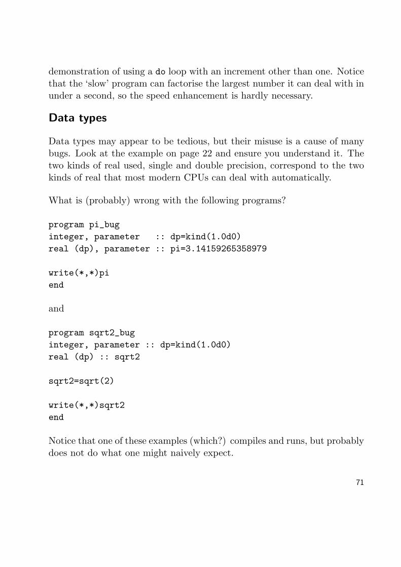
Data types may appear to be tedious, but their misuse is a cause of manybugs. Look at the example on page 22 and ensure you understand it. Thetwo kinds of real used, single and double precision, correspond to the twokinds of real that most modern CPUs can deal with automatically.
What is (probably) wrong with the following programs?
program pi_buginteger, parameter :: dp=kind(1.0d0)real (dp), parameter :: pi=3.14159265358979
write(*,*)piend
and
program sqrt2_buginteger, parameter :: dp=kind(1.0d0)real (dp) :: sqrt2
sqrt2=sqrt(2)
write(*,*)sqrt2end
Notice that one of these examples (which?) compiles and runs, but probablydoes not do what one might naively expect.
71

What does the following program do, and why?
program equalityreal a,binteger i,j
i=123456789j=i+1
a=ib=j
if (i==j) write(*,*)’i==j’if (a==b) write(*,*)’a==b’
end
Which of the following expressions would, according to Fortran, be zero atthe end of the above program?
a-ib-ja-123456789a-123456789.a-123456789d0a-real(i)a-real(i,kind(1.0d0))
In the last expression, real(i,kind(1.0d0)) converts its argument directlyto a double-precision real, rather than the single precision that real(i)produces.
72

Declarations
Look at the example of the variable salery being automatically declaredon page 25. Convince yourself that it really is better if a compiler spotsthese typos rather than accepting them, and therefore that using implicitnone at the beginning of a program is a very good thing.
For the record, neither C nor C++ provide any mechanism for suchautomatic declarations, whereas languages like Basic and Perl use themalmost exclusively.
Arrays
An array can be a very convenient way of storing large amounts of data.A two-dimensional array could be used to store atmospheric temperatureor pressure at ground level on a 10km grid covering the UK. A morecomplicated requirement would be to store wind velocity on a 3D grid. Thiswould require a four-dimensional array, as the velocity itself is a vector.
Try rewriting the simple program on page 12 so that one loop fills an arraywith i, i*i and i**3, and a second loop writes out the contents of thearray.
Look at the example of dynamic arrays on page 31. Can you change theprogram from the above paragraph to prompt for a maximum value for iand to declare an array of the appropriate size? Remember not to deallocatean array before you have finished using it!
More Simple Programs
Herewith some simple programs with no subroutines, functions or libraries.
73

Look at Eratosthenes’ sieve on page 34. Eratosthenes was a Greekmathematician who lived in the third century BC, and invented the well-known method for finding prime numbers. The method is to cross out allmultiples of 2 except 2, all of 3 except 3, all of 4 except 4, etc. The numbersnot struck out are prime.
The program creates the array primes and sets all elements to one.Elements are then struck out by setting them to zero. Finally, the elementsleft are printed.
Try running it for numbers up to about 100 000. You will soon see thatthe calculation time is almost instantaneous, but the time to write outthe answer is quite long! Indeed, you may need to recall that pressing thecontrol key (marked ‘Ctrl’) and ‘C’ together can be useful for aborting suchoutput, although the effect will not be immediate.
One could simply print the highest prime found, by making the final loop
do i=prime_max,2,-1if (primes(i)==1) then
write(*,*)istop
endifenddo
This is now a program which potentially takes more than an instant to run,and which is not delayed by writing to the screen. One can find how longit takes by using the UNIX time command:
bash$ f95 -o sieve eratosthenes_largest.f90bash$ time ./sieveInput largest number for search
74

100009973
0.00user 0.00system 0:02.16elapsed 0%CPU (...)k0inputs+0outputs (128major+36minor)pagefaults 0swaps
That tells us that the program ran for 2.16 seconds of ‘wall-clock’ time, andconsumed 0.00s of CPU (user) time. The difference is the time it took meto enter the number ‘10000’.
However, entering a million makes the user time about 0.87s, ten milliontakes 10.6s, and one hundred million causes the program to run out ofmemory (at least on the machine I was testing this on). Even ten millionwill require forty million bytes (40MB) to hold the array primes, which isbecoming somewhat large, and antisocial on a multiuser machine!
The next program to examine is that to calculate π on page 35. Set trialsto 1000, and run the program a few times. Notice that the answer varies:different random sequences are used each time. If you run the programseveral times in very quick succession (hint: either use the up arrow key torecall the previous command rapidly, or make use of the ‘;’ character whichseparates multiple UNIX commands on the same line, just like FORTRAN,so ‘./pi ; ./pi ; ./pi’ is valid) it gives the same answer each time. Thetime of day is being used to set the initial value produced by the randomnumber generator. This is not good, but getting genuinely random numbersfrom a computer can be hard.
Alter the code so that it prompts for the number of trials. Notice thatalthough the estimates for π get better with increasing numbers of trials,they do so rather slowly. A million trials get three figures fairly reliably,and ten million four figures.
Notice too that although the code becomes rather slow when several milliontrials are requested, the memory use stays constant and tiny: there are no
75

large arrays here. The use of an integer for the loop counter restricts us toabout two thousand million trials, which would take around 10 minutes ona fastish PC.
Some compilers produce code which gives the same ‘random’sequence each time it is run. This can be very useful for debugging.Though the default in Fortran is undefined, either behaviour canbe explicitly requested by setting the seed the generator uses. Thefollowing code is usually good enough.
integer i(1)i(1)=...call random_seed(put=i)
sets the seed. Set i(1) to a constant for the same sequence eachtime, or use
integer i,j(1)call system_clock(i)j(1)=icall random_seed(put=j)
for a different sequence each time.The potential problem with the above code is that the seed is notnecessarily an integer array of length one: some compilers mayrequire a longer integer array. The sort of seed a given compileruses can be determined usingcall random seed(i)which sets i (an integer) to the length of the array of integers whichconstitutes a seed. It is almost always one, and certainly is for thecompiler used for this course. Completely correct code would be:
integer, allocatable :: seed(:)integer icall random_seed(i) ! Get size of seed array
76

allocate(seed(i))! Next line if same sequence each time desiredseed=1! Next two lines if different sequence each time desiredcall system_clock(i)seed=icall random_seed(put=seed)deallocate(seed)
The next example (on page 36) is given in a particularly trivial form: thatof working out what to do in the morning. However, (why) is
call random_number(x)die=1+6*x
the correct code for setting die to a random integer between 1 and 6, thussimulating the roll of a normal six-sided die?
The final example program in this section is that which calculates factorials(see page 37). Why is n declared integer, but fact double precision real?What is the largest number this program can cope with? Does the programstop or produce wrong answers for larger inputs?
Structured Programming
So far our programs have had a very simple structure: just a single pieceof code, with, perhaps, some loops or conditional statements. Now we shallconsider breaking our code into independent self-contained pieces, and thusintroduce the concepts of functions and subroutines. First we considerdefining a function to calculate factorials, just like the previous exampleprogram.
77

The example concerned is on page 38, and looks somewhat complex. Trydeleting the four lines:
module fact_modcontainsend moduleuse fact_mod
and adding the linereal (kind(1.0d0)) :: factorialimmediately after the program test statement.
This reduces the program to something close to Fortran77 syntax, and itwill still compile and run.
The points to notice are that the name of the function is unique withinthe program, and that within the function itself the function name isdeclared just like any other variable, and has values assigned to it like anyother variable. The value of that variable when execution reaches the endfunction statement, or when it reaches a return statement, is the value thefunction returns. The current function returns one for all negative inputs.If one wished it to return −1 to indicate the error, one could add
if (n<0) thenfactorial=-1return
endif
before (or after) the loop. Notice that the variables i and n in the functionare not the same as variables of the same name in the main program.
The addition of the module (the four lines which are potentially removeable)serves an important purpose. It encourages the compiler to check that we
78

are calling our function correctly: that is we are passing it one integer valueand we expect a double precision value back. The NAG compiler used inthis course is quite good at checking itself when it is able, but many othercompilers do not unless the language requires them to do so. The modulealso serves to declare the name factorial within the main program, so itshould not be (re)declared explicitly here anymore. It is good practice touse modules.
Even the NAG compiler will fail to do argument checking if we choseto split this program into two input files without using a module.With the module, it is perfectly reasonable. Simply create two files,the first containing the lines up to and including the end modulestatement, the second containing the main program. Then compileusing:$ f95 -c file1.f90$ f95 -o myprog file2.f90 file1.oNotice the first command will create two files, one calledfact mod.mod and one called file1.o. The first is required bythe use fact mod statement in the main program. It containsinformation about the definition of the factorial function (i.e. thatit wants an integer and returns a double precision). The secondcontains the actual factorial function in compiled binary form.
A subroutine is very like a function, except that it returns no value. It may,however, modify any of the variables passed to it. It is usual practice to usea function only if the routine is to return a single value and print nothing,and to use a subroutine otherwise. A function thus restricted behaves verymuch like all the other functions which one is used to: log, sin, etc.
Look at the example of using a subroutine on page 41. Consider that wheni and j are passed to the subroutine, actually the locations in memorywhich hold i and j are passed. Thus the subroutine can modify them, by
79

storing new values there before it returns. However, as the contents of thememory will be just a collection of binary bits, it is important to ensurethat one passes the correct type to the subroutine. If the subroutine is toldto expect a four-byte integer, and you have actually stored an eight-bytedouble precision real at the address, the subroutine has no way of knowingthis, and strange things will occur. Correct use of modules will preventmost of this chaos, as the compiler will notice and complain.
Libraries
The climax of this course, and most of the problems, is successfully callinga library. This is the sane way to write code: break your task down intogeneral tasks most (all?) of which have been solved before, and call therelevant routines. This you have already been doing to a large extent: ifyou wish to evaluate sin(2.6) you write sin(2.6). You do not worryabout reducing 2.6 to the first quadrant and then looking up some excitingpolynomial or polynomial fraction which will usefully approximate the sinefunction in this region: that is all done for you. The library functionswe shall consider now are more complex and comprehensive than sine, butconceptually similar.
The first example on page 44 simply calls NAG’s identifaction routine. TheFortran starts with a use statement, for modules are provided describing allNAG routines. It then calls the subroutine a00aaf which asks the libraryto identify itself. Unfortunately all NAG routines have these bizarrelyunmemorable names. Notice that as a00aaf takes no arguments, not evenbrackets are needed after its name.
When compiling we must ask the compiler to look in the NAG library forany functions or subroutines we have called and yet not provided code forourselves. This is done with the ‘-lnag’ on the end of the compile line. Theresult should be roughly as shown: try it.
80

A more worth-while example is given starting on page 49. Finding adeterminant is actually quite hard: there are several simple algorithmswhich are algebraically correct, but which do not cope well when executedwith the limited precision and range of a computer’s arithmetic. Suchproblems rarely occur with small matrices, but do readily occur once thematrix has even a few tens of rows and columns. The people at NAG willhave produced a solver which is both fairly robust and which gives an errorif it finds the problem too hard (rather than simply giving a wrong answer).
The NAG documentation talks about LU factorisation and partial pivoting.It is not the purpose of this part of this course to explain or worry aboutsuch techniques.
It then describes in detail what parameters should be passed to the routine,and what it will return. Remember that when a matrix is passed toa subroutine, all the subroutine is given is the address in memory atwhich the first element of that matrix is stored. Thus it is necessary topass separately information about how large a matrix to expect. (Thus‘traditional’ languages like C and Fortran77. More ‘modern’ languages,such as C++ and Fortran90, are capable of passing a single complex objectsuch as an array complete with size and shape information. Unfortunatelythe library which it has been decreed we shall use was written for Fortran77.In some ways this is an advantage: the language is simpler, and no ‘magic’is occurring behind one’s back.)
NAG’s library offers three choices of error detection, which are chosen bysetting the value ifail on entry. These are:ifail=-1 print error message and continueifail=0 print error message and stopifail=1 continueIf you choose ifail to be other than zero, it is essential to check its valueafter calling the NAG routine. Any value apart from zero at this point
81

means that some form of error occurred (i.e. on success the NAG routinewill reset it to zero).
The final examples
The most complex examples in this course, which certainly go as far asyou will need to solve any of the problems set, are those which call aNAG routine which itself needs a user-defined function or subroutine as anargument. The first example is on page 54, where we determine numericallythe maximum of the function xe−x.
Careful reading of the NAG documentation is always required to ensurethat the function or subroutine provided by the user does precisely whatthe library requires. In this case the subroutine is easily written. The NAGroutine itself has a large number of arguments. This is not unreasonable:when performing numerical minimisation, integration, root finding, etc.,one often wishes to trade off speed against accuracy, and NAG thereforeprovides mechanisms for specifying the required accuracy. For a problemthis simple, using the defaults is quite reasonable. NAG also expects ahint as to where to look for the minimum. Again, this is very useful: oursubroutine would fail if called to evaluate the function at x = −10000(why?), but, by telling NAG to look for a minimum between 0.5 and 1.5we get a guarantee that NAG will not ask for the function to be evaluatedoutside of this range.
Try modifying the program to find that minimum of the sinc(x) function(defined as sin(x)/x) which lies between 3 and 5. Try also calling your sincfunction at x = 0: what trap exists here? Notice that unlike the previousexample, this minimisation is rather hard if attempted algebraically.
As a prelude to the final NAG example, we consider one further use ofmodules. So far a module has contained either a function or a subroutine,and the module name and function / subroutine name must be distinct.
82

In fact a module may contain multiple functions and subroutines and alsovariables (including parameters). Thus one can have a module containingthe value of π or h̄ and include it whenever one needs that constant. Asimple example is given on page 55. By using modules in this fashion wecan arrange that certain identically-named variables in the main programand a subroutine (or in multiple functions / subroutines) are identical. Thiscan be very useful as we shall see in the final NAG example.
That final example is to evaluate numerically
I =
Z ∞
−∞e−λx2
dx
for values of λ from 0.1 to 2 in steps of 0.1.
NAG has a routine for doing integration over an infinite or semi-infiniteinterval, at least for functions as well-behaved as this one, and, as usual, wecan specify the precision we require and we are required to provide someworkspace. However, NAG wishes to call a function of x only, and we wishto define a function of λ and x. This is resolved by letting NAG vary xin the obvious manner, and using a module to contain λ. By using thismodule both in our main program and the function, λ is shared betweenthe two without the NAG routine knowing, or needing to know, anythingabout it.
The analytic result of
I2
= 2π
Z ∞
0xe−λx2
dx
= π/λ
83

is familiar. Change the program to print both the numerical result and theresult of evaluating directly
pπ/λ.
Debugging
Bugs are inevitable and unpleasant. Try experimenting with the threedebugging techniques mentioned starting at page 59.
Usually an error of ‘segmentation fault (or violation)’ or ‘sigsegv’ means thatan array bound has been exceeded, whereas a ‘floating point (or numeric orarithmetic) exception’ or ‘sigfpe’ means that an impossible piece of floatingpoint arithmetic (e.g. division by zero, square root of negative number,exponentiation of something large) has been attempted.
Change the gaussian integration routine so that the function readsgaussian=1/exp(lambda*x**2)and investigate the crash which will follow.
For instance, adding:write(*,*)lambda,xproduces the output:
0.1000000000000000 1.00000000000000000.1000000000000000 -1.00000000000000000.1000000000000000 2.3306516868994831E+02
*** Arithmetic exception: - abortingAborted (core dumped)
In other words, NAG requested function evaluations at x = 1, x = −1and x = 233.065. Calculating exp(5431) is (far) beyond the permittedrange of about 10308.
NAG’s compiler also has the useful option ‘-gline’ which causes thefollowing output:
84

*** Arithmetic exception: - abortingfile: gaussian_bug.f90, line 10Aborted (core dumped)
Using the debugger results in the following:
$ f95 -g90 -o bug2 gaussian_bug.f90 -lnag$ dbx90 bug2NAGWare dbx90 Version 4.1(15)Copyright 1995-2000 The Numerical Algorithms Group Ltd.(dbx90) run
Program received signal SIGFPE, Arithmetic exception.(dbx90) where[C] __exp(x) at line 45 in "w_exp.c"
GAUSS_MOD‘GAUSSIAN(GAUSS_MOD‘GAUSSIAN‘X) at line 10in "gaussian_bug.f90"
[C] d01amz_()[C] d01amv_()[C] d01amf_()
INTEGRATE(argc, argv) at line 26 in "gaussian_bug.f90"[C] __libc_start_main(...) at line 129 in "libc-start.c"(dbx90) upCurrent scope is GAUSS_MOD‘GAUSSIAN(dbx90) list 10,1010 gaussian=1/exp(lambda*x**2)(dbx90) print xX = 233.06516868994831(dbx90) print lambdaLAMBDA = 0.10000000000000001(dbx90) print lambda*x*xLAMBDA*X*X = 5431.9372856474065
85

(dbx90) quit$
This tells us that the program died whilst attempting the numericallyimpossible
Program received signal SIGFPE, Arithmetic exception.
and that this was in a routine called exp for which there is no sourceavailable. Typing where shows the current call stack. Our program (main)called d01amf (no surprise there: we did call the NAG routine d01amf).It then called d01amv and d01amz before calling GAUSS MOD MPG̀AUSSIAN,which is our gaussian function with its name embellished to show that itis contained in the gauss mod module. This called exp and the programdied.
By typing up we ask the debugger to move its attention one step up thisstack, that is from the exp function to our gaussian function. We can nowlist the line which called exp, and print the values of x and lambda, or evensimple expressions involving these (however note ** for exponentiation isnot understood by the debugger).
Note that not all bugs cause programs to fail, or even to produce obviouslywrong answers.
86

The format statement
An incomplete list of options to the format statement for reference.
ix integer, at most x charactersix.y integer, at most x characters
and at least y (padded with leading zeros)fx.y floating point, at most x characters and
precisely y characters after the decimal pointex.y exponential, at most x characters and
precisely y characters after the decimal pointdx.y ditto, but use ‘D’ not ‘E’ to represent exponenta ASCII stringax ASCII string, at most x charactersgx.y general – treated as fx.y for numbers close to one,
as ex.y otherwise, and as ix if used on an integer’any text’ literal text
Complex numbers are printed by using two e, f, g or d descriptors.
Any of the above may be preceded by a repeat count.
Examples:
complex cwrite(*,10) c
10 format(f10.4,’ + ’,f10.4,’i’)
integer iwrite(*,10)i,i*i,i**3
10 format(3i8)
integer iwrite(*,10)’Number ’,i,’ your time is up.’
10 format(a,i3,a)
87

The open statement
An incomplete list of options to the open statement for reference.
open(x, file=cc, status=stat, action=act)
x unit number. Integer expression.cc file name. Character variable or constant.stat one of: ’OLD’ (file must exist)
’NEW’ (file must not exist)’REPLACE’ (file will be overwritten)
status=stat is optional.act one of: ’READ’ (writes will not be permitted)
’WRITE’ (reads will not be permitted)’READWRITE’ (no restrictions)
action=act is optional.
Unit numbers 5 and 6 should not be used: 5 often corresponds to reading from the terminal(read(*,*)), 6 to writing to it (write(*,*)).
Simple examples:
open(10,file=’output.dat’)open(50,file=’more.data’,status=’REPLACE’)
Complicated example (ignore if you wish):
character(len=40) nameinteger ii=20
write(name,10)i10 format(’output’,i3.3,’.dat’) ! OK for 0-999 except 5 and 6
open(i,file=name,status=’REPLACE’)
(You have not formally been introduced to the character type, nor using write to fill it)
88

The read statement
The following shows how to read a file of unknown length, and introduces a few new features.The file is assumed to contain two columns of reals, and will be stored in the array x.
integer i,lenreal dummyreal, allocatable :: x(:,:)
open(15,file=’input.dat’,status=’OLD’)len=0 ! Number of lines read succesfullydo
read(15,*,end=20,err=30) dummylen=len+1
enddo
20 rewind(15)allocate (x(2,len))do i=1,len
read(15,*,err=30) x(1,i),x(2,i)enddoclose(15)write(*,*)len,’ data elements read’stop
30 write(*,*)’I/O error occurred’end
The first loop reads in the file, looking for one data item on each line, which it discards bystoring it in the variable dummy, which is overwritten on every cycle of the loop. The end=option of read tells the program to jump to label 20 when it reaches the end of the input file.
The rewind statement tells the program to go back to the beginning of the file for that unitnumber. Originally files would have been stored on tapes, hence the concept of rewind.
Now the number of lines is known, one can allocate an array to hold the data, and read inprecisely the correct number of items. In the case that a line does not start with two itemswhich can be interpreted as reals, an error will occur and the program will jump to label 30.
89

F90 Functions
An incomplete list of F90 functions for reference.
Notation: i – integer, r – real, d – double precision, c – complex, z – double precisioncomplex.Unless otherwise stated, functions return the same type and kind as their argument.
abs(irdcz) Absolute valueacos(rdcz) Arccosineaimag(cz) Imaginary partaint(rd) Truncate to integeranint(rd) Nearest integerasin(rdcz) Arcsineatan(rdcz) Arctangentatan2(rd,rd) atan2(x,y) is the arctangent of x/yceiling(rd) Ceilingcmplx(ird,ird) a + ib as type ccmplx(ird,ird,kind(1d0)) a + ib as type zconjg(cz) Complex conjugatecos(rdcz) Cosinecosh(rdcz) Hyperbolic cosineexp(rdcz) Exponential functionfloor(rd) Floorint(rd) Convert to integer type by truncationlog(rdcz) Natural logarithmlog10(rdcz) Base 10 logarithmmod(i,i) mod(a,b) is a modulo bnint(rd) Convert to nearest integerreal(idcz) Convert to real (r)real(ircz,kind(1d0)) Convert to real (d)sin(rdcz) Sinesinh(rdc) Hyperbolic sinesqrt(rdcz) Square roottan(rdcz) Tangenttanh(rdcz) Hyperbolic tangent
See also page 33 for functions taking arrays as arguments.
90

Reading F77
It is useful to be able to read Fortran77, and here are described those features of F77 whichare best not used in F95, even though they are still valid syntax.
Fixed Form Source
The most striking and archaic feature of F77 is its fixed form source. A comment isindicated by the letter ‘C’ in the first column of a line, the first five columns may containonly statement labels, the sixth column contains the continuation mark (if column six doesnot contain a space, then this line should be considered a continuation of the previous one),and columns seven to seventy-two contain the ‘real’ statements. This made sense in a worldof punched cards, but not today.
Conditionals
The conditional operators <, <=, ==, >=, > and /= are .lt., .le., .eq., .ge., .gt.and .ne. respectively. The characters < and > simply do not occur in F77.
Labels everywhere
We have used statement labels for format statements only. In F77 they were used morewidely. Indeed, the only do loop was of the form
do 10, i=1,20write(*,*)i,i*i
10 continue
The continue statement does nothing, except act as a placeholder for the label. The labelspecified immediately after the do is the last line within the body of the loop. Sometimesone will see the (bad) style of:
do 15, i=1,10do 15, j=1,10
15 a(i,j)=0.0
91

F77 also makes use of the goto statement, which causes execution to jump immediatelyto the label given.
20 write(*,*)’Input a positive number’read(*,*) iif (i.lt.0) goto 20
The goto statement is considered ugly and untidy. It is almost always better to use a do,a multi-line if or a select statement instead.
double precision
Double precision variables could be declared asdouble precision xequivalent to the F90 declarationreal (kind(1.d0)) :: x
Officially this was the only way of specifying double precision, and double precision complexsimply did not exist! Most compilers accepted real*8 as an alternate way of declaringdouble precision reals, and complex*16 for the complex variety.
parameter statement
The declarationinteger iparameter (i=5)is equivalent to the F90 declarationinteger, parameter :: i=5
common
The common statement allows specified variables to be shared by subroutines without beingexplicitly passed. It does nothing useful that modules do not do in a less error-pronefashion.
92

F95 Omissions
Many features of F95 have been intentionally omitted from this course. Time is limited,and the features covered should be quite sufficient for the purposes of this course. However,should you know of other features, you are free to use them.
So that a fair impression of the language is given, here is a list of the main omissions:
• Pointers• User-defined data types• Optional arguments to functions / subroutines• intent attribute for arguments• Private members of modules• Array subobjects (automatic array slicing)• Unformatted I/O (very necessary for large files)• Operator overloading• Recursion• Bit manipulation functions• String handling
93

F95 Syntax summary
A brief and rather incomplete summary of those bits of Fortran syntax covered in thesenotes. This is really intended for those already familiar with a programming language. Ifyou have never programmed before, do not worry if these pages make no sense whatsoever.
Notation: stmnt one F90 statement, stmnts zero or more F90 statements, expr numericexpression, const expression which can be evaluated at compile time, cond condition (logicalexpression), [] enclose optional constructions.
General Structure
module module namecontainsvariable declarationsfunction and subroutine declarationsend module
programuse statementsimplicit nonevariable declarationsstmntsend
There may be zero or multiple modules.
The program statement may carry a name, and the end may be written asend program program name
Names (of modules, functions and variables) can be up to 31 characters, case insensitive,first character alphabetic, others alphanumeric or underscore.
94
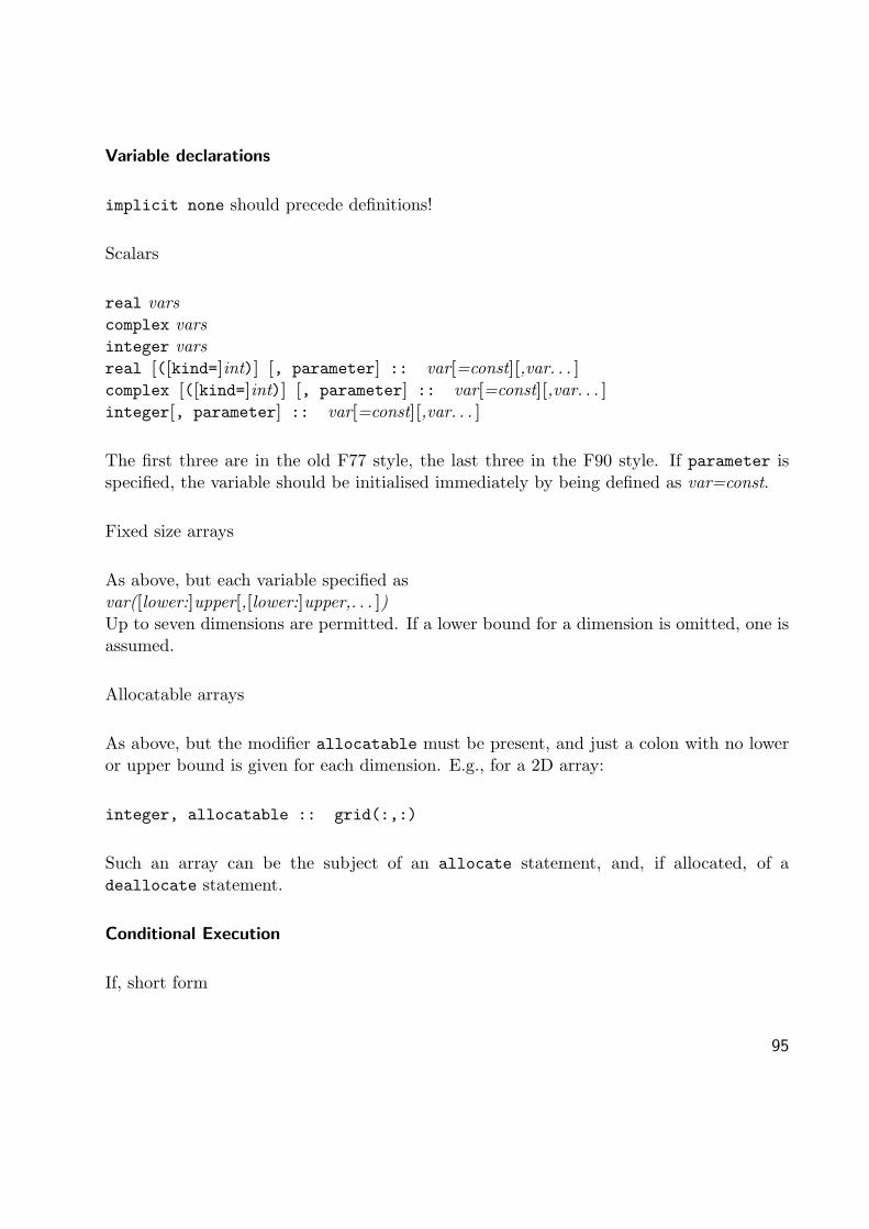
Variable declarations
implicit none should precede definitions!
Scalars
real varscomplex varsinteger varsreal [([kind=]int)] [, parameter] :: var[=const][,var. . . ]complex [([kind=]int)] [, parameter] :: var[=const][,var. . . ]integer[, parameter] :: var[=const][,var. . . ]
The first three are in the old F77 style, the last three in the F90 style. If parameter isspecified, the variable should be initialised immediately by being defined as var=const.
Fixed size arrays
As above, but each variable specified asvar([lower:]upper[,[lower:]upper,. . . ])Up to seven dimensions are permitted. If a lower bound for a dimension is omitted, one isassumed.
Allocatable arrays
As above, but the modifier allocatable must be present, and just a colon with no loweror upper bound is given for each dimension. E.g., for a 2D array:
integer, allocatable :: grid(:,:)
Such an array can be the subject of an allocate statement, and, if allocated, of adeallocate statement.
Conditional Execution
If, short form
95

if (cond) stmnt
If, long form
if (cond) thenstmnts[else if (cond) thenstmnts][elsestmnts]end if
Any number of else if clauses may occur.
Select
select case (expr)case (const[:const][,const])stmnts[case defaultstmnts ]end select
Where const:const denotes a range, and commas separate multiple single values or ranges.The range may be open-ended, such as ‘:5’ for anything less than or equal to five.
Loops
do var=expr1,expr2[,expr3][stmnts][if ( cond ) exit][stmnts]enddo
var must be defined as an integer variable, and will take the value expr1 for the firstiteration of the loop, and have expr3 added to it at the end of each iteration. If expr3is omitted, it is taken to be one. The total number of iterations is floor(1+(expr2-expr1)/expr3), or zero if this is negative. The expressions must be integer, and will be
96

evaluated just once on entry to the loop. No attempt may be made to change the value ofvar within the loop.
do[stmnts]if ( cond ) exit[stmnts]enddo
An infinite loop. Some form of exit is effectively required.
97

Bibliography
The following resources may be helpful, and were used in preparing this course.
FORTRAN 90/95 explained, Metcalf and Reid, Oxford Science Publications, £18.Fortran 90 for Scientists and Engineers, Hahn, Arnold, £23.
Metcalf and Reid covers the language only, Hahn also includes some background onnumerical methods. As neither is cheap, you may prefer to seek out library copies.
(Fortran 90 and Fortran 95 are almost indistinguishable: do not worry if a book mentionsF90 only).
The course WWW site, found from http://www.phy.cam.ac.uk/, or, more directly, athttp://www.mrao.cam.ac.uk/teaching/comp phy/, has some pointers to other usefulF90 resources too, as well as an errata for this document, should one be needed.
98
!, 17**, 7:, 31::, 21;, 22=, 6, 11==, 11&, 17
algebra, 8allocatable, 31allocate, 31ANSI, 3antisocial, 75argument, 8, 18argument passing, 42array
bounds, 29, 61functions, 33operations, 32
arrays, 27–29, 73dynamic, 31static, 31
assignment, 6, 11
Bell Labs, 3
calculator, 68call, 42case, 36case sensitivity, 7close, 58comments, 17, 65common, 92comparison, 11, 91complex, 19, 23complex, 23conditions, 10constants, 9, 18, 20contains, 38continuation line, 17continue, 91conversions, 24core files, 64
dbx90, 62, 64, 85deallocate, 31debugger, 62, 85debugging, 59–64, 84declarations, 17, 18, 73
99

do, 12, 14, 16, 34, 91double precision, 92
elements, 29end, 5, 31, 38, 58enddo, 12endif, 10Eratosthenes, 34, 74examples, copying, 68executable, 67exit, 14exponents, 20expression, 18external, 53
f95, 5-g90, 62, 85-gline, 84-lnag, 44, 80
factorials, 37, 38factorisation, 15file I/O, 58, 88, 89format, 13, 70, 87Fortran 77, 91function, 8, 18
function, 38functions, 39, 78
list of, 90
goto, 92
IBM, 3if, 10, 34ifail, 81implicit declarations, 25implicit loops, 32implicit none, 26, 65indentation, 10, 65indices, 29, 30input, 8integer, 19integer, 6integers, 7
kind, 21
label, 13, 89, 91libraries, 43, 80linker, 43loops, 12, 14, 32
memory usage, 30
100
mod, 15module, 38modules, 39, 79
variables in, 55
NAG compiler, 79NAG library, 43–54
documentation, 45numerical integration, 56
omissions, 93open, 58, 88operator, 18
parameter, 9, 92π, 35portability, 2precidence, 8precision, 19, 21, 22, 72print, 5program, 38
random numbers, 35, 75random number, 35random seed, 76range, 19, 20, 70
read, 8, 89real, 19real, 8, 15, 72real*8, 92rewind, 89run-time checks, 61
scalar, 27select case, 36selected real kind, 21SIGFPE, 84, 86SIGSEGV, 84speed, 71, 75sqrt, 8, 15, 23, 71stop, 10stride, 34subroutine, 41subroutines, 42, 52, 79subscripts, 29supercomputers, 4
test, 53, 65, 84time, 74type conversions, 24
101

ulimit, 64unit number, 58use, 38
variable, 18variables, 6, 7, 65vectors, 27
write, 58, 88
102