Embed Size (px)
Citation preview

Fortran 90 & 95Array and Pointer
TechniquesObjects, Data Structures, and Algorithms
with subsets e-LF90 and F
DO NOT COPYThis document was downloaded from
www.fortran.com/fortranon a single-print license agreement
Making copies without written permissionconstitutes copyright violation.
Further information may be obtained from Unicomp, Inc. at11930 Menaul Blvd. NE, Suite 106; Albuquerque, NM 87112 USA; (505) 323-1758.
Loren P. Meissner
Computer Science DepartmentUniversity of San Francisco

Fortran 90 & 95Array and Pointer
TechniquesObjects, Data Structures, and Algorithms
with subsets e-LF90 and F
Loren P. Meissner
Computer Science Department
University of San Francisco
Copyright 1998, Loren P. Meissner
16 September 1998
Copyright © 1998 by Loren P. Meissner. All rights reserved. Except as permitted under the United StatesCopyright Act of 1976, no part of this book may be reproduced or distributed in any form or by anymeans, or stored in a database or retrieval system without the prior written permission of the author.


ContentsContents
Preface
Chapter 1 Arrays and Pointers 11.1 WHAT IS AN ARRAY? 1
SubscriptsMultidimensional ArraysArrays as ObjectsWhole Arrays and Array Sections
Whole Array OperationsElemental Intrinsic FunctionsArray SectionsArray Input and OutputStandard Array Element SequenceArray Constructors and Array-Valued ConstantsVector Subscripts
1.2 ARRAY TECHNIQUES 11Operation Counts and Running Time
Operation Counts for Swap SubroutineThe Invariant Assertion MethodSmallest Element in an Array Section
Operation Counts for Minimum_LocationSearch in an Ordered Array
Linear Search in an Ordered ArrayBinary Search in an Ordered ArrayOperation Counts for Binary_Search
Solving Systems of Linear Algebraic EquationsSome Details of Gauss EliminationCrout FactorizationIterative Refinement
1.3 POINTERS 36The Pointer Attribute
Association StatusAutomatic DereferencingThe deallocate Statement
Storage for Pointers and Allocated TargetsManagement of Allocated Targets
Pointers as Derived Type ComponentsPointers with Arrays
iii
Chapter 2 Introduction to Sorting 42Computer Sorting
Operation Counts for Sort_32.1 SORTING BY SELECTION 44
Operation Counts for Selection SortSorting an Array of StructuresSelection during OutputDuplicate Keys
Selection Sort is not Stable2.2 SORTING BY INSERTION 52
Straight InsertionOperation Counts for Straight InsertionInitially Ordered DataStraight Insertion Is Stable
Insertion Sort with PointersInsertion during Input
Expanding ArrayBinary Insertion
Binary Insertion Is Not StableOperation Counts for Binary Insertion
2.3 SHELL SORT 62Operation Counts for Shell SortShell Sort with Array Sections
2.4 HEAPSORT 64Binary Trees (Array Representation) and HeapsThe Procedure PeckBuilding the Heap by Chain InsertionSorting the Heap by Selection
Operation Counts for Heapsort2.5 OPERATION COUNTS FOR SORTING: SUMMARY 75
Sorting Methods Described So Far (Slower to Faster)
Chapter 3 Recursion and Quicksort 773.1 RECURSION 77
Recursion Compared with IterationA Good Example of Recursion: Towers of HanoiA Bad Example of Recursion: The Fibonacci SequenceApplication: Adaptive Quadrature (Numerical Integration)Application: Recursive Selection SortTail Recursion vs Iteration
Printing a List ForwardFactorial
3.2 QUICKSORT 76Recursive Partitioning
Quicksort is Unstable for DuplicatesChoosing the PivotThe Cutoff
Testing a Quicksort ImplementationStorage Space ConsiderationsQuicksort Operation Counts
iv
Chapter 4 Algorithm Analysis 944.1 WHAT IS AN ALGORITHM? 94
Computer Algorithms4.2 WHAT MAKES A GOOD ALGORITHM? 95
From Thousands to Millions of Data ItemsOperation Counts for Sorting
4.3 ASYMPTOTIC ANALYSIS 97The Role of ConstantsThe Complexity of an Algorithm: Big OhComplexity of Sorting Methods
4.4 MATHEMATICAL INDUCTION 101
Chapter 5 Linked Lists 1025.1 LINKED LIST NODE OPERATIONS 102
Create ListInsert Target NodeDelete Target NodePrint Target NodeModify Target Node
5.2 OPERATIONS ON WHOLE LINKED LISTS 106Making a Linked List by Insertion at the RootPrint ListDelete ListSearching in a Linked ListMaintaining a Large Ordered List
5.3 PROCESSING LINKED LISTS RECURSIVELY 1095.4 LINKED LISTS WITH POINTERS TO POINTERS 1135.5 APPLICATIONS WITH SEVERAL LINKED LISTS 118
Multiply Linked Lists5.6 LINKED LISTS VS. ARRAYS 119
Array ImplementationUnordered ArrayOrdered Array
Linked List ImplementationUnordered Linked ListOrdered Linked List
Summary
v
Chapter 6 Abstract Data Structures 1216.1 STACKS 121
Applications of StacksDepth-First Search in a GraphStack OperationsEvaluating a Postfix ExpressionStacks and RecursionRecursive Depth-First SearchReversing a List
Abstraction, Encapsulation, and Information HidingStack as an Object
Array Implementation of StackLinked List Implementation of Stack
A Stack of What?Generic Stack Module
Stack Objects6.2 QUEUES 137
Queue ObjectsLinked List Implementation of QueueArray Implementation of QueueSpecial Considerations for High Efficiency
Chapter 7 Trees 1457.1 BINARY SEARCH TREES 145
The Balance Problem7.2 AVL TREES 149
Rotating a Subtree7.3 B-TREES 1537.4 SKIP LISTS 1577.5 COMPARISON OF ALGORITHMS 162
Index 165
vi
PrefaceThis book covers modern Fortran array and pointer techniques, including facilities provided by Fortran95, with attention to the subsets e-LF90 and F as well. It provides coverage of Fortran based data struc-tures and algorithm analysis.
The principal data structure that has traditionally been provided by Fortran is the array. Data struc-turing with Fortran has always been possible — although not always easy: one of the first textbooks onthe subject (by Berztiss, in 1971) used Fortran for its program examples. Fortran 90 significantly ex-tended the array features of the language, especially with syntax for whole arrays and array sectionsand with many new intrinsic functions. Also added were data structures, pointers, and recursion. Mod-ern Fortran is second to none in its support of features required for efficient and reliable implementationof algorithms and data structures employing linked lists and trees as well as arrays.
Examples shown in this book use some features of Fortran 95, notably derived type componentinitialization, pointer initialization with null , and pure functions. Electronically distributed programexamples include the Fortran 95 versions printed in the book, as well as alternative versions acceptableto the Fortran 90 subsets e-LF90 and F. Each of these subsets supports all essential features of Fortran 90but omits obsolete features, storage association, and many redundancies that are present in the fullFortran language; furthermore, they are available at a very reasonable price to students and educators.Information concerning e-LF90 (“essential Lahey Fortran 90”) is available from Lahey Computer Sys-tems, Inc.; 865 Tahoe Blvd.; Incline Village, NV 89450; (702) 831-2500; <www.lahey.com> ;<[email protected]> . Information concerning the F subset is available from Imagine1; 11930 MenaulBlvd. NE, Suite 106; Albuquerque, NM 87112; (505) 323-1758; <www.imagine1.com/imagine1> ;<[email protected]> .
The programming style used in this book, and in all three electronically distributed variant versionsof the programming examples, is close to that required by F (the more restrictive of the two subsets). Fversion examples conform to the “common subset” described in essential Fortran 90 & 95: Common SubsetEdition, by Loren P. Meissner (Unicomp, 1997), except that short-form read and print statements re-place the more awkward form that common subset conformance requires. The e-LF90 version examplesincorporate extensions described in Appendix C of essential Fortran, namely: initialization and type defi-nition in the main program, simple logical if statements, do while , and internal procedures. Fortran95 version examples (including those printed in the text) do not employ any further extensions exceptfor facilities that are new in Fortran 95. All versions of the examples have been tested; the Fortran 95versions were run under DIGITAL Visual Fortran v 5.0c: see <www.digital.com/ fortran> .
Bill Long, Clive Page, John Reid, and Chuckson Yokota reviewed earlier drafts of this material andsuggested many improvements.
vii

1
Chapter 1 Arrays and Pointers
1.1 WHAT IS AN ARRAY?Think of a group of objects that are all to be treated more or less alike — automobiles on an assemblyline, boxes of Wheaties on the shelf at a supermarket, or students in a classroom. A family with five or sixchildren may have some boys and some girls, and their ages will vary over a wide range, but the chil-dren are similar in many ways. They have a common set of parents; they probably all live in the samehouse; and they might be expected to look somewhat alike.
In computer applications, objects to be processed similarly may be organized as an array. Fortran isespecially noted for its array processing facilities. Most programming languages including Ada, C, andPascal provide statements and constructs that support operations such as the following:• Create an array with a given name, shape, and data type
• Assign values to one or more designated elements of an array
• Locate a specific element that has been placed in the array
• Apply a specified process to all elements of a particular array, either sequentially (one element at atime) or in parallel (all at once).Two important properties make arrays useful.
1. An array is a homogeneous collection — all of its elements are alike in some important ways. In pro-gramming language terms, all elements of a given array have the same data type.1 This has twoconsequences:
First, it means that all elements of an array permit the same operations — those that are definedfor the data type. For example, if the array elements are integers, operations of arithmetic such asaddition and multiplication can be performed upon them. If their data type is logical, the applicableoperations include and, or, and not.
Second, having a common data type implies that all the elements of a given array have the samestorage representation. The elements each occupy the same amount of space, which means that theycan be stored in a linear sequence of equal-sized storage areas.
2. Each element is identified by a sequential number or index. Along with the fact that each elementoccupies some known amount of space in computer storage, this means that the addressing mecha-nisms in the computer hardware can easily locate any element of a particular array when its indexnumber is known. A process to be applied to the array elements can proceed sequentially accordingto the index numbers, or a parallel process can rely upon the index numbers to organize the way inwhich all elements are processed.
1 A Fortran data type can have type parameters. All elements of a given array have the same data type and thesame type parameters.
2
SubscriptsIn mathematical writing, the index number for an array element appears as a subscript — it is written ina smaller type font and on a lowered type baseline: A1 for example. Most programming languages,including Fortran, have a more restricted character set that does not permit this font variation, so theindex number is enclosed in parentheses that follow the array name, as A(1) . Some languages usesquare brackets instead of parentheses for the array index, as A[1] . Regardless of the notation, arrayindices are called subscripts for historical reasons.
A subscript does not have to be an integer constant such as 1, 17 , or 543 ; rather, in most contexts itcan be an arbitrary expression of integer type. For example, the array element name Ai+1 is written inFortran as A(I + 1) . The value of a subscript expression is important, but its form is not. A specific arrayelement is uniquely identified (at a particular point in a program) by the name of the array along with thevalue of the subscript. The subscript value is applied as an ordinal number (first, second, third, . . .) todesignate the position of a particular element with relation to others in the array element sequence.
In the simplest case, subscripts have positive integer values from 1 up to a specific upper bound; forexample, the upper bound is 5 in an array that consists of the elements
A(1) A(2) A(3) A(4) A(5)
The lower bound may have a different value, such as 0 or –3 in the following arrays:A(0) A(1) A(2) A(3) A(4)A(-3) A(-2) A(-1) A(0) A(1)
In any case, the subscript values consist of consecutive integers ranging from the lower bound to theupper bound.2 The extent is the number of different permissible subscript values; the extent is 5 in eachof the foregoing examples. More generally (for consecutive subscripts), the extent is the upper boundplus one minus the lower bound.
It should be noted that an array can consist of a single element: its upper and lower bounds can bethe same. Perhaps surprisingly, Fortran (like a few other programming languages) permits an array tohave no elements at all. In many contexts, such an array is considered to have lower bound 1 and upperbound 0.
Multidimensional ArraysAn array may be multidimensional, so that each element is identified by more than one subscript. Therank of an array is the number of subscripts required to select one of the elements. A rank-2 array is two-dimensional and is indexed by two subscripts; it might have six elements:
B(1, 1) B(2, 1) B(3, 1) B(1, 2) B(2, 2) B(3, 2)
On paper, a one-dimensional array is usually written as a sequence of elements from left to right,such as any of the arrays named A in the previous examples. A two-dimensional array can be displayedas a matrix in which the first subscript is invariant across each row and the second subscript is invariantdown each column, as in mathematics:
B(1, 1) B(1, 2) B(1, 3)B(2, 1) B(2, 2) B(2, 3)
There is no convenient way to display an array of three or more dimensions on a single sheet ofpaper. A three-dimensional array can be imagined as a booklet with a matrix displayed on each page.The third subscript is invariant on each page, while the first two subscripts designate the row and col-umn of the matrix on that page.
2 Array subscripts are normally consecutive. Special Fortran array section notation supports nonconsecutivesubscript values.
Arrays and Pointers
3
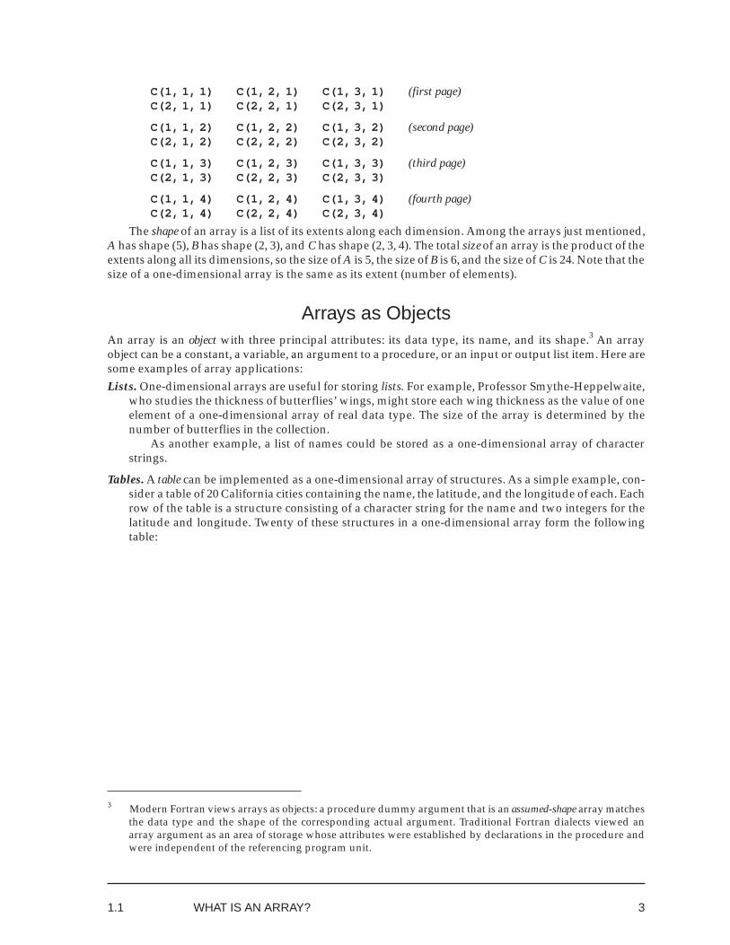
C(1, 1, 1) C(1, 2, 1) C(1, 3, 1) (first page)C(2, 1, 1) C(2, 2, 1) C(2, 3, 1)
C(1, 1, 2) C(1, 2, 2) C(1, 3, 2) (second page)C(2, 1, 2) C(2, 2, 2) C(2, 3, 2)
C(1, 1, 3) C(1, 2, 3) C(1, 3, 3) (third page)C(2, 1, 3) C(2, 2, 3) C(2, 3, 3)
C(1, 1, 4) C(1, 2, 4) C(1, 3, 4) (fourth page)C(2, 1, 4) C(2, 2, 4) C(2, 3, 4)
The shape of an array is a list of its extents along each dimension. Among the arrays just mentioned,A has shape (5), B has shape (2, 3), and C has shape (2, 3, 4). The total size of an array is the product of theextents along all its dimensions, so the size of A is 5, the size of B is 6, and the size of C is 24. Note that thesize of a one-dimensional array is the same as its extent (number of elements).
Arrays as ObjectsAn array is an object with three principal attributes: its data type, its name, and its shape.3 An arrayobject can be a constant, a variable, an argument to a procedure, or an input or output list item. Here aresome examples of array applications:Lists. One-dimensional arrays are useful for storing lists. For example, Professor Smythe-Heppelwaite,
who studies the thickness of butterflies’ wings, might store each wing thickness as the value of oneelement of a one-dimensional array of real data type. The size of the array is determined by thenumber of butterflies in the collection.
As another example, a list of names could be stored as a one-dimensional array of characterstrings.
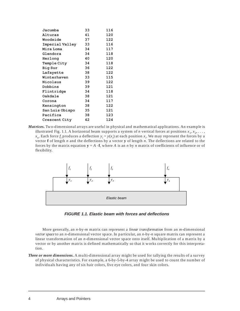
Tables. A table can be implemented as a one-dimensional array of structures. As a simple example, con-sider a table of 20 California cities containing the name, the latitude, and the longitude of each. Eachrow of the table is a structure consisting of a character string for the name and two integers for thelatitude and longitude. Twenty of these structures in a one-dimensional array form the followingtable:
3 Modern Fortran views arrays as objects: a procedure dummy argument that is an assumed-shape array matchesthe data type and the shape of the corresponding actual argument. Traditional Fortran dialects viewed anarray argument as an area of storage whose attributes were established by declarations in the procedure andwere independent of the referencing program unit.
1.1 WHAT IS AN ARRAY?
4
Jacumba 33 116Alturas 41 120Woodside 37 122Imperial Valley 33 116Mira Loma 34 117Glendora 34 118Herlong 40 120Temple City 34 118Big Sur 36 122Lafayette 38 122Winterhaven 33 115Nicolaus 39 122Dobbins 39 121Flintridge 34 118Oakdale 38 121Corona 34 117Kensington 38 122San Luis Obispo 35 121Pacifica 38 123Crescent City 42 124
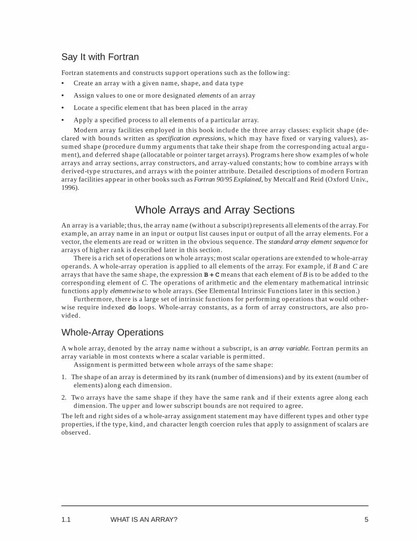
Matrices. Two-dimensional arrays are useful in physical and mathematical applications. An example isillustrated Fig. 1.1. A horizontal beam supports a system of n vertical forces at positions x1, x2, . . . ,xn. Each force fi produces a deflection yi = y(xi) at each position xi. We may represent the forces by avector f of length n and the deflections by a vector y of length n. The deflections are related to theforces by the matrix equation y = A· f, where A is an n by n matrix of coefficients of influence or offlexibility.
Elastic beam
f1 f2 f3 fn
y1 y2 y3 yn
FIGURE 1.1. Elastic beam with forces and deflections
More generally, an n-by-m matrix can represent a linear transformation from an m-dimensionalvector space to an n-dimensional vector space. In particular, an n-by-n square matrix can represent alinear transformation of an n-dimensional vector space onto itself. Multiplication of a matrix by avector or by another matrix is defined mathematically so that it works correctly for this interpreta-tion.
Three or more dimensions. A multi-dimensional array might be used for tallying the results of a surveyof physical characteristics. For example, a 6-by-5-by-4 array might be used to count the number ofindividuals having any of six hair colors, five eye colors, and four skin colors.
Arrays and Pointers
5
Say It with Fortran
Fortran statements and constructs support operations such as the following:• Create an array with a given name, shape, and data type
• Assign values to one or more designated elements of an array
• Locate a specific element that has been placed in the array
• Apply a specified process to all elements of a particular array.Modern array facilities employed in this book include the three array classes: explicit shape (de-
clared with bounds written as specification expressions, which may have fixed or varying values), as-sumed shape (procedure dummy arguments that take their shape from the corresponding actual argu-ment), and deferred shape (allocatable or pointer target arrays). Programs here show examples of wholearrays and array sections, array constructors, and array-valued constants; how to combine arrays withderived-type structures, and arrays with the pointer attribute. Detailed descriptions of modern Fortranarray facilities appear in other books such as Fortran 90/95 Explained, by Metcalf and Reid (Oxford Univ.,1996).
Whole Arrays and Array SectionsAn array is a variable; thus, the array name (without a subscript) represents all elements of the array. Forexample, an array name in an input or output list causes input or output of all the array elements. For avector, the elements are read or written in the obvious sequence. The standard array element sequence forarrays of higher rank is described later in this section.
There is a rich set of operations on whole arrays; most scalar operations are extended to whole-arrayoperands. A whole-array operation is applied to all elements of the array. For example, if B and C arearrays that have the same shape, the expression B + C means that each element of B is to be added to thecorresponding element of C. The operations of arithmetic and the elementary mathematical intrinsicfunctions apply elementwise to whole arrays. (See Elemental Intrinsic Functions later in this section.)
Furthermore, there is a large set of intrinsic functions for performing operations that would other-wise require indexed do loops. Whole-array constants, as a form of array constructors, are also pro-vided.
Whole-Array Operations
A whole array, denoted by the array name without a subscript, is an array variable. Fortran permits anarray variable in most contexts where a scalar variable is permitted.
Assignment is permitted between whole arrays of the same shape:
1. The shape of an array is determined by its rank (number of dimensions) and by its extent (number ofelements) along each dimension.
2. Two arrays have the same shape if they have the same rank and if their extents agree along eachdimension. The upper and lower subscript bounds are not required to agree.
The left and right sides of a whole-array assignment statement may have different types and other typeproperties, if the type, kind, and character length coercion rules that apply to assignment of scalars areobserved.
1.1 WHAT IS AN ARRAY?
6
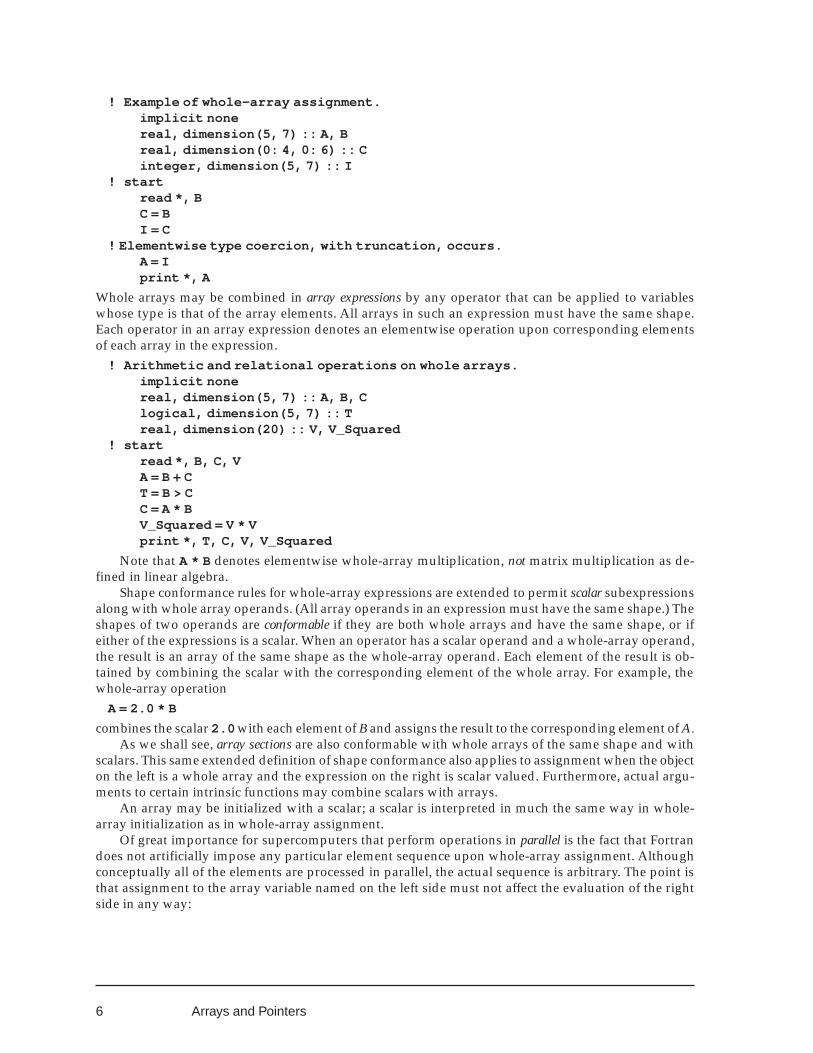
! Example of whole-array assignment.implicit nonereal, dimension(5, 7) :: A, Breal, dimension(0: 4, 0: 6) :: Cinteger, dimension(5, 7) :: I
! startread *, BC = BI = C
! Elementwise type coercion, with truncation, occurs.A = Iprint *, A
Whole arrays may be combined in array expressions by any operator that can be applied to variableswhose type is that of the array elements. All arrays in such an expression must have the same shape.Each operator in an array expression denotes an elementwise operation upon corresponding elementsof each array in the expression.
! Arithmetic and relational operations on whole arrays.implicit nonereal, dimension(5, 7) :: A, B, Clogical, dimension(5, 7) :: Treal, dimension(20) :: V, V_Squared
! startread *, B, C, VA = B + CT = B > CC = A * BV_Squared = V * Vprint *, T, C, V, V_Squared
Note that A * B denotes elementwise whole-array multiplication, not matrix multiplication as de-fined in linear algebra.
Shape conformance rules for whole-array expressions are extended to permit scalar subexpressionsalong with whole array operands. (All array operands in an expression must have the same shape.) Theshapes of two operands are conformable if they are both whole arrays and have the same shape, or ifeither of the expressions is a scalar. When an operator has a scalar operand and a whole-array operand,the result is an array of the same shape as the whole-array operand. Each element of the result is ob-tained by combining the scalar with the corresponding element of the whole array. For example, thewhole-array operation
A = 2.0 * B
combines the scalar 2.0 with each element of B and assigns the result to the corresponding element of A.As we shall see, array sections are also conformable with whole arrays of the same shape and with
scalars. This same extended definition of shape conformance also applies to assignment when the objecton the left is a whole array and the expression on the right is scalar valued. Furthermore, actual argu-ments to certain intrinsic functions may combine scalars with arrays.
An array may be initialized with a scalar; a scalar is interpreted in much the same way in whole-array initialization as in whole-array assignment.
Of great importance for supercomputers that perform operations in parallel is the fact that Fortrandoes not artificially impose any particular element sequence upon whole-array assignment. Althoughconceptually all of the elements are processed in parallel, the actual sequence is arbitrary. The point isthat assignment to the array variable named on the left side must not affect the evaluation of the rightside in any way:
Arrays and Pointers
7
real, dimension(L) :: First, Second:
First = First + Second
A possible model for whole-array assignment assumes a temporary “array-sized register,” or shadowof the left side, whose elements are assigned as they are calculated. As a final step, the shadow registeris copied into the designated left side array. It is important to note, however, that whole-array assign-ment can often be implemented without incurring the extra space or time penalties implied by thismodel.
Elemental Intrinsic Functions
Many intrinsic functions, notably including the mathematical functions, are classified as elemental. Anelemental intrinsic function accepts either a scalar or an array as its argument. When the argument is anarray, the function performs its operation elementwise, applying the scalar operation to every arrayelement and producing a result array of the same shape. For elemental intrinsic functions with morethan one array argument, all actual arguments that are arrays must have the same shape. The followingstatements apply the intrinsic functions max and sin elementwise to whole arrays:
implicit nonereal, dimension(5, 7) :: A, B, C, Dlogical, dimension(5, 7) :: T
:A = max( B, C )C = max( A, 17.0 )T = sin( A ) > 0.5
Array Sections
An especially useful feature permits operations on all the elements in a designated portion of an array.An array section is permitted in most situations that accept a whole array. Most operations that are validfor scalars of the same type may be applied (elementwise) to array sections as well as to whole arrays. Inparticular, an array section may be an actual argument to an elemental intrinsic function.
The simplest form of array section is a sequence of consecutive elements of a vector. Such an arraysection is designated by the array name followed by a pair of subscript expressions that are separated bya colon and represent the subscript limits of the array section. Either expression (but not the colon) maybe omitted; the default limits are the declared array bounds:
real, dimension(40) :: Bakerreal, dimension(5, 17) :: Johnreal, dimension(144) :: Able
:Baker(1: 29)Baker(: 29) ! Default lower limit is 1.John(5: 11)John(: 11) ! Default is declared lower bound.Able(134: 144)Able(134: ) ! Default is declared upper bound.
An array section may be combined in an expression with whole arrays or other array expressions (ofthe same shape) and with scalars, and it may appear on the left side in an assignment statement. Each ofthe following assignment statements moves a consecutive subset of the elements of a vector.
real, dimension(100) :: Xreal, dimension(5) :: Y, ZX(1: 50) = X(51: 100)Y(2: 5) = Y(1: 4)Z(1: 4) = Z(2: 5)
1.1 WHAT IS AN ARRAY?
8
An array section designator may include a third expression. This increment (in this context, oftencalled the stride) gives the spacing between those elements of the underlying parent array that are to beselected for the array section:
real, dimension(8) :: Areal, dimension(18) :: VA = V(1: 15: 2)
Values assigned to A are those of V1, V3, . . . , V15. A negative increment value reverses the normal arrayelement sequence:
A = B(9: 2: -1)
Here, elements of the reversed array section — the eight elements B9, B8, B7, . . . , B2, in that order — areassigned to the consecutive elements of A.
A more complicated example is the following:real, dimension(3, 5) :: Ereal, dimension(2, 3) :: FF = E(1: 3: 2, 1: 5: 2)
Here, on the last line, the first subscript of E takes on values 1, 3 and the second subscript of E takes onvalues 1, 3, 5. The array section is a two-dimensional array object whose shape matches that of F.
Any of the three components of an array section designator may be omitted. The final colon must beomitted if the third component is omitted:
real, dimension(100) :: AA(: 50) ! Same as A(1: 50) or A(1: 50: 1)A(: 14: 2) ! Same as A(1: 14: 2)A(2: ) ! Same as A(2: 100) or A(2: 100: 1)A(2: : 3) ! Same as A(2: 100: 3)A(: : 2) ! Same as A(1: 100: 2)A(:) ! Same as A(1: 100) or A(1: 100: 1) or AA(: : -1) ! Same as A(1: 100: -1); array section of zero sizeA(1: 100: ) ! Prohibited
The default values for these components are, respectively, the lower subscript bound for the array di-mension, the upper bound for the array dimension, and 1.
Array section designators may be combined with single subscripts to designate an array object oflower rank:
V(: 5) = M(2, 1: 5)
Here, the elements M2,1 through M2,5 form a one-dimensional array section that is assigned to the firstfive elements of V. As another example, A(3, :) designates the third row of the matrix A (all elementswhose first subscript is 3), and A(:, 5) designates the fifth column of the matrix A (all elements whosesecond subscript is 5).
The rank of an array section is the number of subscript positions in which at least one colon appears;a colon in a subscript position signals that there is a range of subscript values for that dimension. Theextent along each dimension is simply the number of elements specified by the section designator forthat dimension.
In the absence of a colon, a fixed subscript value must appear; fixing one subscript value reduces therank by 1. If Fours is an array of rank 4, then Fours(:, :, :, 1) denotes the rank-3 array that consistsof all elements of Fours whose fourth subscript is 1. Fours(:, :, 1, 1) denotes the matrix (rank-2array) that consists of all elements of Fours whose third and fourth subscripts are both 1. Fours(:, 1,1, 1) denotes the vector (rank-1 array) that consists of all elements of Fours whose second, third, andfourth subscripts are all 1. Finally, Fours(1, 1, 1, 1) names a scalar, which, for most purposes, maybe considered a rank-0 array. Note that Fours(1: 1, 1: 1, 1: 1, 1: 1) is not a scalar but an arraywhose rank is 4 and whose size is 1. This latter array may also be denoted as Fours(: 1, : 1, : 1,: 1) .
See also Vector Subscripts, later in this Section.
Arrays and Pointers
9
Array Input and Output
An Input list or an Output list may include a reference to a whole array. The elements are transmittedaccording to a standard sequence, defined immediately below. For an array of rank 1, this sequenceconsists of the elements in increasing subscript order. A rank-one array section without a stride designa-tor also causes transmission of a set of contiguous array elements in increasing subscript order.
! Input and output of whole arrays and array sections.implicit noneinteger, parameter :: ARRAY_SIZE = 5integer, dimension(ARRAY_SIZE) :: Data_Array
! startread *, Data_Array ! Whole arrayprint *, " The first four values: ", Data_Array(: 4) ! Array section
Standard Array Element Sequence
Some operations and intrinsic functions on whole arrays require that a standard element sequence be de-fined. The standard sequence depends on the subscript values: The leftmost subscript is varied first,then the next subscript, and so on.
Let the declaration for an array be
Type , dimension( UBound1 , UBound2 , UBound3 ) :: Array name
Then, a reference to
Array name( Subscript1 , Subscript2 , Subscript3 )
will designate the element whose sequential position is
S1 + U1 · (S2 − 1) + U1 · U2 · (S3 − 1)
where U represents an upper bound value in the declaration and S represents a subscript in the refer-ence.
For arrays with explicit lower subscript bounds as well as upper bounds, the formula of courseinvolves the bound values. If an array is declared with lower bounds L1, L2, L3 and upper bounds U1, U2,U3, and an element is referenced with subscript values S1, S2, S3, the sequential position of this elementis given by the following formula:
1 + (S1 − L1) + (U1 − L1 + 1) · (S2 − L2) + (U1 − L1 + 1) · (U2 − L2 + 1) · (S3 − L3)
This formula can easily be generalized to more than three dimensions.Note that U3, the upper subscript range bound for the last dimension, does not appear in this for-
mula. This last upper bound value has a role in determining the total size of the array, but it has no effecton the array element sequence.
Array Constructors and Array-Valued Constants
Fortran provides a method for constructing a vector by specifying its components as individual expres-sions or expression sequences. An array constructor consists of a List of expressions and implied doloops, enclosed by the symbols (/ and /) :
(/ List /)The expressions in the List may be scalar expressions or array expressions.
Array constructors are surprisingly versatile. For example, two or more vectors may be concat-enated, or joined end to end, with an array constructor. In the following statement, suppose that X, Y,and Z are vectors:
Z = (/ X, Y /)
1.1 WHAT IS AN ARRAY?
10
The usual conformance requirements of array assignment apply. Here, the length of Z must be the sumof the lengths of X and Y, and other attributes of the data must be compatible.
Array constructors are especially useful for constructing array-valued constants, as illustrated bythe following examples. The first two of the following array constructors form constant vectors of realtype, while the third is a constant vector of integer type.
(/ 3.2, 4.01, 6.4 /)(/ 4.5, 4.5 /)(/ 3, 2 /)
A named constant may be a whole array:integer, dimension(5), parameter :: PRIMES = (/ 2, 3, 5, 7, 11 /)
A whole-array variable may be initialized in a type declaration, giving the initial value of the arrayby means of a scalar or an array constructor:
real, dimension(100), save :: Array = 0.0integer,dimension(5), save :: Initial_Primes = (/ 2, 3, 5, 7, 11 /)
The implied do loop form that is permitted in an array constructor is so called because of its resem-blance to the control statement of an indexed do construct:
( Sublist , Index = Initial value , Limit [, Increment ] )For example,
(J + 3, J + 2, J + 1, J = 1, N)
The Sublist consists of a sequence of items of any form that is permitted in the List; an implied do loopmay be included in a sublist within an outer implied do loop. The Index variable (called an array con-structor implied-do variable or ACID variable) should not be used for any other purpose; furthermore,it should be a local variable and should not have the pointer attribute.
Constructing an array of higher rankAn array constructor always creates an array of rank 1, but the intrinsic function reshape can be ap-plied to create an array of higher rank. For example, the following expression constructs an N by Nidentity matrix:
reshape( (/ ((0.0, J = 1, I - 1), 1.0, (0.0, J = I + 1, N), I = 1, N) /), (/ N, N /) )The intrinsic function reshape has two arguments, source and shape . The first argument, source , isan array of rank 1, of any type, with the correct total number of elements. The the second argument,shape , is a vector of one to seven positive integer elements. The number of elements in the shapevector determines the rank of the result from reshape . Each element of shape gives the size along onedimension of the result array; thus, the product of the element values of shape gives the total size of theresult.
integer, parameter :: N = 10integer, dimension(2), parameter :: Y_SHAPE = (/ 3, 2 /), &
Z_SHAPE = (/ N, N /)integer :: I, J ! I and J are ACID variables.real, dimension(2) :: Xreal, dimension(3, 2) :: Yreal, dimension(N * N) :: Qreal, dimension(N, N) :: Z
! startX = (/ 4.5, 4.5 /)Y = reshape( (/ (I + 0.2, I = 1, 3), X, 2.0 /), Y_SHAPE )Q = (/ ((0.0, J = 1, I - 1), 1.0, (0.0, J = I + 1, N), I = 1, N) /)Z = reshape( Q, Z_SHAPE )
Arrays and Pointers
11
Here Y_SHAPE and Z_SHAPE are named array constants. Another array constant is assigned to X. In theassignment to Y, the source argument to the reshape function is an array constructor with six compo-nents: The first three are given by an implied do loop, the next two come from the vector X, and the sixthis the constant 2.0 . An array constructor is assigned to the vector Q, which is then reshaped to form Zand becomes an N by N identity matrix.
Vector Subscripts
A vector of integer type may appear as a subscript in an array section designator, along with any of theother allowed forms. The designated array section is formed by applying the elements of the vectorsubscript in sequence as subscripts to the parent array. Thus, the value of each element of the vectorsubscript must be within the array bounds for the parent array.
For example, suppose that Z is a 5 by 7 matrix and that U and V are vectors of lengths 3 and 4,respectively. Assume that the elements of U and V have the following values:
U 1, 3, 2V 2, 1, 4, 3
Then, Z(3, V) consists of elements from the third row of Z in the following order:Z(3, 2), Z(3, 1), Z(3, 4), Z(3, 3)
Also, Z(U, 2) consists of elements from the second column:Z(1, 2), Z(3, 2), Z(2, 2)
And, Z(U, V) consists of the following elements:Z(1, 2), Z(1, 1), Z(1, 4), Z(1, 3),Z(3, 2), Z(3, 1), Z(3, 4), Z(3, 3),Z(2, 2), Z(2, 1), Z(2, 4), Z(2, 3)
In the most useful applications, the elements of the subscript vector consist of a permutation ofconsecutive integers, as in these examples. The same integer may appear more than once in a subscriptvector, but this practice is error-prone and should be done only with great care.
Vector subscripts are prohibited in certain situations. In particular, an actual argument to a proce-dure must not be an array section with a vector subscript if the corresponding dummy argument arrayis given a value in the procedure. Furthermore, an array section designated by a vector subscript with arepeated value must not appear on the left side of an assignment statement nor as an input list item.
The rank of an array section is the number of subscript positions that contain either a colon or thename of an integer vector (vector subscript). The extent of an array section along each dimension issimply the number of elements specified by the section designator for that dimension. For a vectorsubscript, the extent is determined by the number of elements in the vector.
1.2 ARRAY TECHNIQUESThis section examines some array processing techniques that are generally useful; many of these will beapplied in later chapters.
Operation Counts and Running TimeAn important purpose of this textbook is to compare different methods of accomplishing the same re-sult. Several different factors in this comparison are discussed in Chapter 4, but the major one is runningtime. For numerical work, as in most traditional Fortran “number crunching” applications, running timeis dominated by floating point operations (especially by multiplication time). On the other hand, for thenonnumerical applications that are the subject of this text it is more useful to count comparison opera-tions and move operations.
1.2 ARRAY TECHNIQUES
12
It is assumed here that comparisons and moves account for most of the running time, or else thatthese are typical operations and that total running time is proportional to some combination of these.This assumption is unrealistic in actual practice, of course, for several reasons. First, it ignores the over-head of loop control, procedure reference, etc., which can dominate the “useful” operations in a tightloop or in a short procedure. Furthermore, as Bill Long has pointed out, memory loads are probably amore relevant factor than moves because the processor must wait for their completion, whereas mostprocessors accomplish memory stores asynchronously.
Consider a procedure for exchanging two array elements with the aid of an auxiliary variable. Thisexample illustrates the methods and notation that will be used. Declarations and other nonexecutablestatements are omitted. Line numbers are given at the right for reference.
Operation Counts for Swap Subroutine
Aux = Array(I) ! 1Array(I) = Array(J) ! 2Array(J) = Aux ! 3
The subroutine performs three move operations and no comparisons.If I and J have the same value, Swap accomplishes nothing. At the cost of one comparison, the three
move operations might be saved:if (I /= J) then ! 1
Aux = Array(I) ! 2Array(I) = Array(J) ! 3Array(J) = Aux ! 4
end if ! 5This subroutine always performs one comparison, at line 1, and it sometimes performs three moves.
Which version runs faster? The answer depends upon the relative times of comparison operationsand move operations, and whether the moves are required. Let p be the probability that I and J aredifferent; then the expected operation counts for the second subroutine are one comparison and 3pmoves.
Assuming for the moment that a comparison takes the same amount of time as a move, the firstsubroutine performs three operations and the second performs 3p +1 operations. If p is larger than 0.67,the first subroutine is faster.
For most applications described in this text, swapping an item with itself is rare (p is close to 1) andthe test should be omitted.
However, the relative timing of comparison and move operations can change from one applicationto another. Data base comparisons employ a key that is often a relatively small part of each item; thus themove operation takes considerably longer than the comparison. For some indexed data base applica-tions, however, only pointers are moved, so the move time and comparison time are more nearly equal.For an indexed application with a long key, comparison operations can require more time than moves.
The Invariant Assertion MethodSome array techniques employ a repetitive procedure or loop that can be designed and verified with theaid of an invariant assertion. Consider the following example.
Suppose that you are a bunk bed salesman. Kensington Residential Academy wants to buy newbunk beds for its dormitories, which must be long enough for the tallest student at the Academy. Youneed to find the tallest student so that you can order beds according to his height. So you stand at thedoor of the dining hall as the students file in, one at a time.
How do you proceed? Imagine that you have solved a portion of the problem. Some (but not all) ofthe students have entered, and you have found the tallest student among those who are now in the hall.You have asked this tallest student to stand aside, at the left of the doorway.
Arrays and Pointers
13
One more student enters. What do you have to do to solve this incremental problem? If the nextstudent is taller than the one standing by the door, you ask the next student to stand there instead. If thenext student is not taller, you leave the previous student standing there. Now the tallest student in theslightly larger group is standing by the doorway.
An invariant assertion for an event that occurs repeatedly, such as students entering the dining hallone at a time, is a statement that is true after each repetitive occurrence. For the bunk bed problem, asuitable assertion is the following:
“The tallest student in the dining hall is now standing by the doorway.”An invariant assertion has the following properties:• The assertion must be true initially, before repetition begins.
You must do something special with the first student. When he enters, you ask him to standaside, and you start the repetitive process with the second student.
• Each occurrence of the repetitive process must maintain the validity of the assertion. That is, it canbe verified that if the assertion is true prior to a repetitive step, then it remains true after that step.This is what “invariant” means.
For the bunk bed problem, you check the height of each new student who enters and you re-place the current tallest student if the new one is taller. This guarantees that the assertion remainstrue.
• Validity of the assertion at the end of the repetition describes the goal of the entire process.When all of the students have entered the hall, the process terminates, and the student standing
by the doorway is the tallest of them all.The design of a loop can often be facilitated by trying to find an invariant assertion. This is not
always easy. For array applications, by analogy to the problem of finding the tallest student, it ofteninvolves imagining the situation when a typical section of the array (but not all of it) has been processed.The invariant assertion then tells what should happen when the section is enlarged by one element.
Smallest Element in an Array SectionA procedure for locating the smallest element in a section of an array Array(Lo: Hi) can be con-structed by analogy to the bunk bed problem. The procedure employs a loop to examine portions of thearray section, incorporating one more element at each iteration. At each step, the variable Min_Val recordsthe smallest value among the elements examined so far. The location (subscript value) where the smallestelement was found is also recorded.
An appropriate invariant assertion is:“The variable Min_Val records the smallest element in the current portion of the array,and Loc records the location (subscript value) where it was found.”
The assertion is made true initially by assigning ArrayLo to Min_Val and Lo to Loc.Min_Val = Array(Lo)Loc = Lo
Iteration begins with the element at subscript position Lo + 1. To guarantee the validity of the asser-tion when a new item ArrayI is incorporated, Min_Val is compared with the new item and replaced ifnecessary.
do I = Lo + 1, Hiif (Array(I) < Min_Val) then
Min_Val = Array(I)Loc = I
end ifend do
1.2 ARRAY TECHNIQUES
14
At loop termination, the assertion is:“The variable Min_Val records the smallest element in the entire array section, and Locrecords the location where it was found.”
The array section has grown to encompass the entire array, and the current value of Loc is the desiredresult value.
Operation Counts for Minimum_Location
Min_Val = Array(Lo) ! 1Loc = Lo ! 2do I = Lo + 1, Hi ! 3
if (Array(I) < Min_Val) then ! <4Min_Val = Array(I) ! <5Loc = I ! <6
end if ! <7end do ! <8
The number of data items processed by this function is P = Hi + 1 – Lo. The function includes onecomparison at line 4 and data moves at lines 1 and 5. Only those steps that move an actual data item arecounted. The loop body contains one comparison and one move. The comparison is executed once foreach iteration of the loop, so there are P – 1 comparisons altogether. The expected number of moves(including the extra move at line 1) can be shown to be ∑i=1
P(1/i); lnP + 0.6 approximates this sum.4
Say It with Fortran
Fortran provides standard intrinsic functions minval and minloc , which return the value and locationof the smallest element in an array or array section; corresponding functions maxval and maxloc arealso provided. However, these intrinsic functions can be applied only to arrays of integer or real type;extension to character type is proposed for a future version of Fortran.
Furthermore, coding the operation explicitly illustrates the Fortran techniques involved. The fol-lowing function locates the smallest element in the portion of an array of strings that is bounded bysubscript limits given as the arguments Lo and Hi. The result variable, Loc, is an integer that locates thesmallest element of Array to be found between subscript positions Lo and Hi.
When this function is used, it will inherit a requirement for explicit type declarations from its host. Acalling program will refer to the function by the name Minimum_Location , but within the function theresult value is called Minimum_Location_R .
The keyword pure in a function heading is recognized by Fortran 95 as an assertion that the func-tion has no side effects — i.e., it has no external effects except for returning the result value. This keywordis not recognized by Fortran 90, and the electronically distributed Fortran 90 versions omit it.
4 Paul Zeitz and Chuckson Yokota, private communications. Here, Euler’s constant γ = 0.5772 . . . plus somefurther terms (negligible for large P) in the “harmonic sum” are estimated by the constant 0.6; see D. E. Knuth,Fundamental Algorithms, The Art of Computer Programming, vol. 1 (Reading: Addison-Wesley, 1968), 73ff.
Here ln P is the natural logarithm, base e = 2.718 . . . . Natural logarithms appear rarely in this text; the mostuseful logarithmic base for algorithm analysis is 2. This text uses the notation lg P for the base 2 logarithm ofP. The value of lg P is about 1.44 times the natural logarithm of P or 3.32 times the common (base 10) logarithmof P; a Fortran program can compute lg P from either of the expressions 1.44269504 * log( P ) or 3.32192809* log10( P ) . Twenty-digit values of these constants are log2 e = 1.4426950408889634074 and log2 10 =3.3219280948873623479 (from Mathematica®).
Arrays and Pointers
15
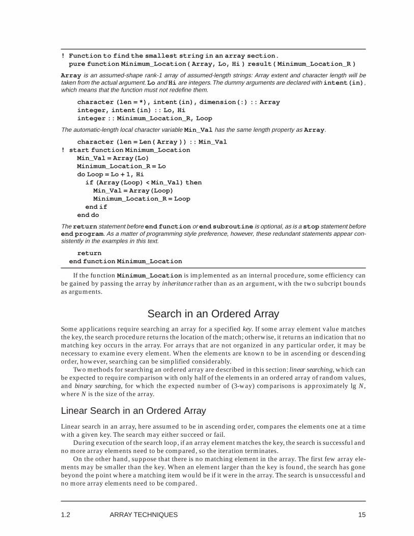
! Function to find the smallest string in an array section.pure function Minimum_Location( Array, Lo, Hi ) result( Minimum_Location_R )
Array is an assumed-shape rank-1 array of assumed-length strings: Array extent and character length will betaken from the actual argument. Lo and Hi are integers. The dummy arguments are declared with intent(in) ,which means that the function must not redefine them.
character (len = *), intent(in), dimension(:) :: Arrayinteger, intent(in) :: Lo, Hiinteger :: Minimum_Location_R, Loop
The automatic-length local character variable Min_Val has the same length property as Array .
character (len = Len( Array )) :: Min_Val! start function Minimum_Location
Min_Val = Array(Lo)Minimum_Location_R = Lodo Loop = Lo + 1, Hi
if (Array(Loop) < Min_Val) thenMin_Val = Array(Loop)Minimum_Location_R = Loop
end ifend do
The return statement before end function or end subroutine is optional, as is a stop statement beforeend program . As a matter of programming style preference, however, these redundant statements appear con-sistently in the examples in this text.
returnend function Minimum_Location
If the function Minimum_Location is implemented as an internal procedure, some efficiency canbe gained by passing the array by inheritance rather than as an argument, with the two subcript boundsas arguments.
Search in an Ordered ArraySome applications require searching an array for a specified key. If some array element value matchesthe key, the search procedure returns the location of the match; otherwise, it returns an indication that nomatching key occurs in the array. For arrays that are not organized in any particular order, it may benecessary to examine every element. When the elements are known to be in ascending or descendingorder, however, searching can be simplified considerably.
Two methods for searching an ordered array are described in this section: linear searching, which canbe expected to require comparison with only half of the elements in an ordered array of random values,and binary searching, for which the expected number of (3-way) comparisons is approximately lg N,where N is the size of the array.
Linear Search in an Ordered Array
Linear search in an array, here assumed to be in ascending order, compares the elements one at a timewith a given key. The search may either succeed or fail.
During execution of the search loop, if an array element matches the key, the search is successful andno more array elements need to be compared, so the iteration terminates.
On the other hand, suppose that there is no matching element in the array. The first few array ele-ments may be smaller than the key. When an element larger than the key is found, the search has gonebeyond the point where a matching item would be if it were in the array. The search is unsuccessful andno more array elements need to be compared.
1.2 ARRAY TECHNIQUES
16
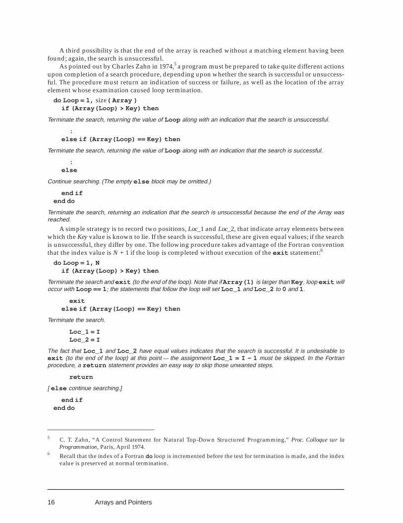
A third possibility is that the end of the array is reached without a matching element having beenfound; again, the search is unsuccessful.
As pointed out by Charles Zahn in 1974,5 a program must be prepared to take quite different actionsupon completion of a search procedure, depending upon whether the search is successful or unsuccess-ful. The procedure must return an indication of success or failure, as well as the location of the arrayelement whose examination caused loop termination.
do Loop = 1, size( Array )if (Array(Loop) > Key) then
Terminate the search, returning the value of Loop along with an indication that the search is unsuccessful.
:else if (Array(Loop) == Key) then
Terminate the search, returning the value of Loop along with an indication that the search is successful.
:else
Continue searching. (The empty else block may be omitted.)
end ifend do
Terminate the search, returning an indication that the search is unsuccessful because the end of the Array wasreached.
A simple strategy is to record two positions, Loc_1 and Loc_2, that indicate array elements betweenwhich the Key value is known to lie. If the search is successful, these are given equal values; if the searchis unsuccessful, they differ by one. The following procedure takes advantage of the Fortran conventionthat the index value is N + 1 if the loop is completed without execution of the exit statement:6
do Loop = 1, Nif (Array(Loop) > Key) then
Terminate the search and exit (to the end of the loop). Note that if Array(1) is larger than Key , loop exit willoccur with Loop == 1; the statements that follow the loop will set Loc_1 and Loc_2 to 0 and 1.
exitelse if (Array(Loop) == Key) then
Terminate the search.
Loc_1 = ILoc_2 = I
The fact that Loc_1 and Loc_2 have equal values indicates that the search is successful. It is undesirable toexit (to the end of the loop) at this point — the assignment Loc_1 = I - 1 must be skipped. In the Fortranprocedure, a return statement provides an easy way to skip those unwanted steps.
return
[ else continue searching.]
end ifend do
Arrays and Pointers
5 C. T. Zahn, “A Control Statement for Natural Top-Down Structured Programming,” Proc. Colloque sur laProgrammation, Paris, April 1974.
6 Recall that the index of a Fortran do loop is incremented before the test for termination is made, and the indexvalue is preserved at normal termination.
17
The fact that Loc_1 and Loc_2 have unequal values indicates that the search is unsuccessful. Note that ifArray(N) is smaller than Key , the loop will terminate normally with Loop == N +1; Loc_1 and Loc_2 will beset to N and N +1.
Loc_1 = I - 1Loc_2 = I
The invariant assertion method can be applied to this problem; an appropriate assertion is:1 ≤ Loop ≤ N +1 and ArrayLoop–1 ≤ Key < ArrayN+1
For this analysis, imagine that there is an extra fictitous array element at each end: Array0 with avery large negative value and ArrayN+1 with a very large positive value. (These fictitious elements arenot actually created as part of the array, and they are never referenced by program statements. Theironly role is in the invariant assertion.)
Taking into account the fictitious array elements, the assertion is true when Loop is initialized to 1 byloop contol processing. Because the array is in ascending order, Arrayi ≤ Arrayj whenever 0 ≤ i ≤ j ≤ N + 1.
The return statement in the if construct is executed only if a match is found. The exit statementis executed (and Loop is preserved) if ArrayLoop > Key; normal loop termination (with Loop = N + 1, byFortran convention) occurs if Key > ArrayN. In either of these two latter cases, the statement followingend do is reached with 1 ≤ Loop ≤ N + 1 and ArrayLoop–1 ≤ Key < ArrayLoop.
Say It with Fortran
The following Fortran function implements linear search for a Key among the elements of an array ofcharacter strings. One detail has been changed because a Fortran function can return an array but itcannot return two separate scalars. The two bracketing subscript values (named Loc_1 and Loc_2 in theforegoing discussion) are combined into a vector named Linear_Search_R.
! Linear search in an ordered array.pure function Linear_Search( Array, Key ) result( Linear_Search_R )
Array is an assumed-shape rank-1 array of assumed-length strings; Key is an assumed-length string. Extentand character length of Array and character length of Key will be taken from the corresponding actual argu-ments.
character (len = *), intent(in), :: Array(:), Keyinteger, dimension(2) :: Linear_Search_R
! start function Linear_Searchdo Loop = 1, size( Array )
if (Array(Loop) > Key) thenexit
else if (Array(Loop) == Key) then
The following statement assigns a scalar value to both vector elements.
Linear_Search_R = Loopreturn
end ifend doLinear_Search_R(1) = Loop - 1Linear_Search_R(2) = Loopreturn
end function Linear_Search
1.2 ARRAY TECHNIQUES

18
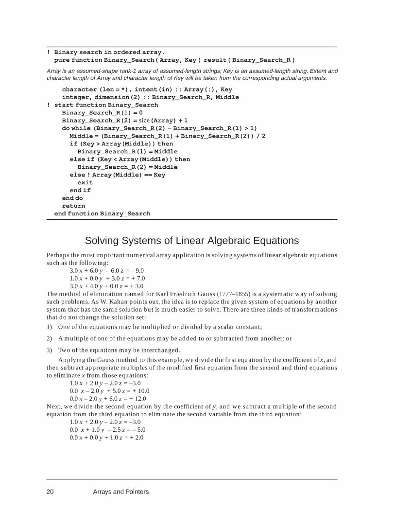
Binary Search in an Ordered Array
For a large ordered array, a binary search is much more efficient than the linear search just described. Theidea of this method is to cut the search area in two at each step by finding out whether the key value isin the left half or the right half of the array. Since the array elements are in order, this determination canbe made by examining just one element in the middle of the array. The selected half is again bisected,either the left half or the right half is chosen, and the process continues. The search area is ultimatelyreduced either to a single element that matches the key or else to two adjacent elements between whichthe key value lies.
Each time the search area is bisected, only one (3-way) comparison of the key with an array elementis required. (As explained in the discussion of Operation Counts below, a 3-way comparison is equiva-lent, on the average, to 1.5 simple comparisons.) Therefore, the total number of comparisons, and thetotal number of repetitions of the loop, is proportional to lg N where N is the array size. A linear searchin an ordered array of 10,000 elements may be expected to require some 5,000 comparisons, but a binarysearch never requires more than 15 three-way comparisons (or 21 simple comparisons). See also Exer-cise 6 at the end of this section.
The invariant assertion method can be applied to this problem. Let the variables Loc_1 and Loc_2contain the index values of array elements between which the Key value is known to lie. It is possible, ofcourse, that the key value is smaller or larger than all elements of the array. Again, the invariant asser-tion assumes fictitous elements Array0 with a very large negative value and ArrayN+1 with a very largepositive value. An appropriate assertion is:
0 ≤ Loc_1 ≤ Loc_2 ≤ N + 1 and ArrayLoc_1 ≤ Key ≤ ArrayLoc_2The assertion is made true initially by setting Loc_1 to 0 and Loc_2 to N + 1. The fact that the array is
in ascending order implies that Arrayi ≤ Arrayj whenever 0 ≤ i ≤ j ≤ N + 1.The loop is executed while the difference Loc_2 – Loc_1 is greater than 1. This difference measures
the extent of the subscript range that currently encloses the Key value:7
Loc_1 = 0Loc_2 = N + 1do while (Loc_2 - Loc_1 > 1)
Middle = (Loc_2 + Loc_1) / 2:
end do
At each iteration, the subscript range that encloses Key is bisected and either Loc_1 or Loc_2 is set toMiddle to preserve the invariant assertion. However, it may happen that ArrayMiddle exactly matches thesearch key. In this case, there is no further need to continue bisecting the array, so the loop is terminated:
Loc_1 = 0Loc_2 = N + 1do while (Loc_2 - Loc_1 > 1)
Middle = (Loc_1 + Loc_2) / 2if (Key > Array(Middle)) then
Loc_1 = Middleelse if (Key < Array(Middle)) then
Loc_2 = Middle
7 Recall that Fortran integer division truncates the true quotient. If Loc_1 + Loc_2 is an even integer, the quotientis exact; if odd, the expression value is the next integer smaller than the true quotient. When Loc_1 and Loc_2are some distance apart, a slight change in the bisection point has little effect. However, careful analysis isrequired when the two values are close together.
Arrays and Pointers
19
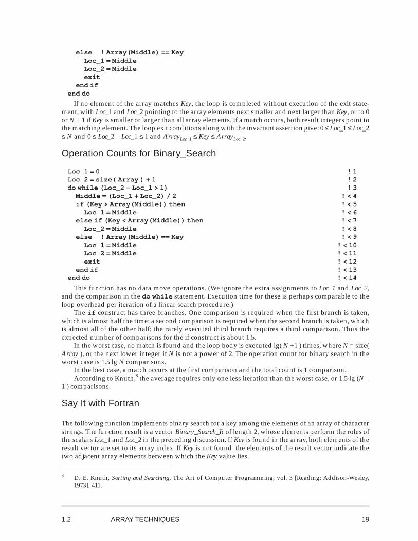
else ! Array(Middle) == KeyLoc_1 = MiddleLoc_2 = Middleexit
end ifend do
If no element of the array matches Key, the loop is completed without execution of the exit state-ment, with Loc_1 and Loc_2 pointing to the array elements next smaller and next larger than Key, or to 0or N + 1 if Key is smaller or larger than all array elements. If a match occurs, both result integers point tothe matching element. The loop exit conditions along with the invariant assertion give: 0 ≤ Loc_1 ≤ Loc_2≤ N and 0 ≤ Loc_2 – Loc_1 ≤ 1 and ArrayLoc_1 ≤ Key ≤ ArrayLoc_2.
Operation Counts for Binary_Search
Loc_1 = 0 ! 1Loc_2 = size( Array ) + 1 ! 2do while (Loc_2 - Loc_1 > 1) ! 3
Middle = (Loc_1 + Loc_2) / 2 ! < 4if (Key > Array(Middle)) then ! < 5
Loc_1 = Middle ! < 6else if (Key < Array(Middle)) then ! < 7
Loc_2 = Middle ! < 8else ! Array(Middle) == Key ! < 9
Loc_1 = Middle ! < 10Loc_2 = Middle ! < 11exit ! < 12
end if ! < 13end do ! < 14
This function has no data move operations. (We ignore the extra assignments to Loc_1 and Loc_2,and the comparison in the do while statement. Execution time for these is perhaps comparable to theloop overhead per iteration of a linear search procedure.)
The if construct has three branches. One comparison is required when the first branch is taken,which is almost half the time; a second comparison is required when the second branch is taken, whichis almost all of the other half; the rarely executed third branch requires a third comparison. Thus theexpected number of comparisons for the if construct is about 1.5.
In the worst case, no match is found and the loop body is executed lg( N +1 ) times, where N = size(Array ), or the next lower integer if N is not a power of 2. The operation count for binary search in theworst case is 1.5 lg N comparisons.
In the best case, a match occurs at the first comparison and the total count is 1 comparison.According to Knuth,8 the average requires only one less iteration than the worst case, or 1.5·lg (N –
1 ) comparisons.
Say It with Fortran
The following function implements binary search for a key among the elements of an array of characterstrings. The function result is a vector Binary_Search_R of length 2, whose elements perform the roles ofthe scalars Loc_1 and Loc_2 in the preceding discussion. If Key is found in the array, both elements of theresult vector are set to its array index. If Key is not found, the elements of the result vector indicate thetwo adjacent array elements between which the Key value lies.
1.2 ARRAY TECHNIQUES
8 D. E. Knuth, Sorting and Searching, The Art of Computer Programming, vol. 3 [Reading: Addison-Wesley,1973], 411.
20
! Binary search in ordered array.pure function Binary_Search( Array, Key ) result( Binary_Search_R )
Array is an assumed-shape rank-1 array of assumed-length strings; Key is an assumed-length string. Extent andcharacter length of Array and character length of Key will be taken from the corresponding actual arguments.
character (len = *), intent(in) :: Array(:), Keyinteger, dimension(2) :: Binary_Search_R, Middle
! start function Binary_SearchBinary_Search_R(1) = 0Binary_Search_R(2) = size(Array) + 1do while (Binary_Search_R(2) - Binary_Search_R(1) > 1)
Middle = (Binary_Search_R(1) + Binary_Search_R(2)) / 2if (Key > Array(Middle)) then
Binary_Search_R(1) = Middleelse if (Key < Array(Middle)) then
Binary_Search_R(2) = Middleelse ! Array(Middle) == Key
exitend if
end doreturn
end function Binary_Search
Solving Systems of Linear Algebraic EquationsPerhaps the most important numerical array application is solving systems of linear algebraic equationssuch as the following:
3.0 x + 6.0 y – 6.0 z = – 9.01.0 x + 0.0 y + 3.0 z = + 7.03.0 x + 4.0 y + 0.0 z = + 3.0
The method of elimination named for Karl Friedrich Gauss (1777–1855) is a systematic way of solvingsuch problems. As W. Kahan points out, the idea is to replace the given system of equations by anothersystem that has the same solution but is much easier to solve. There are three kinds of transformationsthat do not change the solution set:1) One of the equations may be multiplied or divided by a scalar constant;
2) A multiple of one of the equations may be added to or subtracted from another; or
3) Two of the equations may be interchanged.Applying the Gauss method to this example, we divide the first equation by the coefficient of x, and
then subtract appropriate multiples of the modified first equation from the second and third equationsto eliminate x from those equations:
1.0 x + 2.0 y – 2.0 z = –3.00.0 x – 2.0 y + 5.0 z = + 10.00.0 x – 2.0 y + 6.0 z = + 12.0
Next, we divide the second equation by the coefficient of y, and we subtract a multiple of the secondequation from the third equation to eliminate the second variable from the third equation:
1.0 x + 2.0 y – 2.0 z = –3.00.0 x + 1.0 y – 2.5 z = – 5.00.0 x + 0.0 y + 1.0 z = + 2.0
Arrays and Pointers
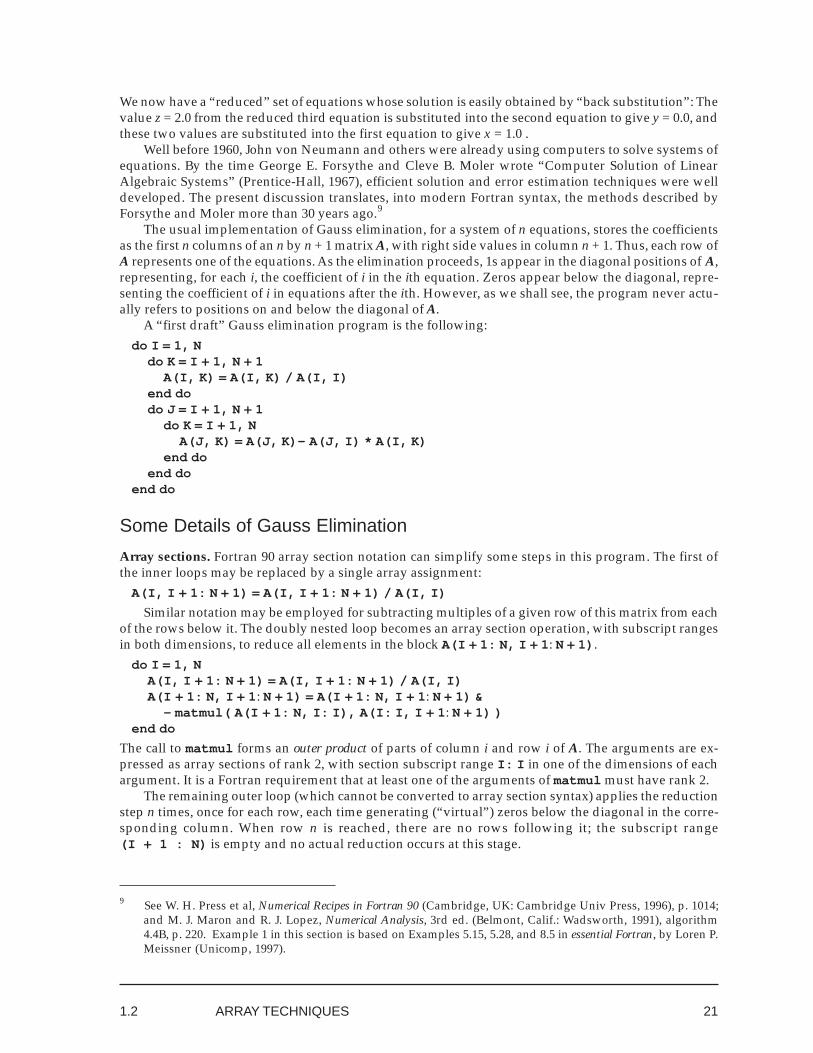
21
We now have a “reduced” set of equations whose solution is easily obtained by “back substitution”: Thevalue z = 2.0 from the reduced third equation is substituted into the second equation to give y = 0.0, andthese two values are substituted into the first equation to give x = 1.0 .
Well before 1960, John von Neumann and others were already using computers to solve systems ofequations. By the time George E. Forsythe and Cleve B. Moler wrote “Computer Solution of LinearAlgebraic Systems” (Prentice-Hall, 1967), efficient solution and error estimation techniques were welldeveloped. The present discussion translates, into modern Fortran syntax, the methods described byForsythe and Moler more than 30 years ago.9
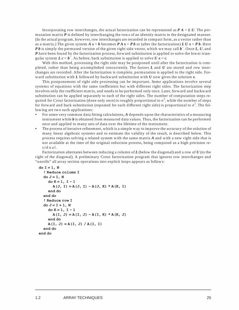
The usual implementation of Gauss elimination, for a system of n equations, stores the coefficientsas the first n columns of an n by n + 1 matrix A, with right side values in column n + 1. Thus, each row ofA represents one of the equations. As the elimination proceeds, 1s appear in the diagonal positions of A,representing, for each i, the coefficient of i in the ith equation. Zeros appear below the diagonal, repre-senting the coefficient of i in equations after the ith. However, as we shall see, the program never actu-ally refers to positions on and below the diagonal of A.
A “first draft” Gauss elimination program is the following:do I = 1, N
do K = I + 1, N + 1A(I, K) = A(I, K) / A(I, I)
end dodo J = I + 1, N + 1
do K = I + 1, NA(J, K) = A(J, K)- A(J, I) * A(I, K)
end doend do
end do
Some Details of Gauss Elimination
Array sections. Fortran 90 array section notation can simplify some steps in this program. The first ofthe inner loops may be replaced by a single array assignment:
A(I, I + 1: N + 1) = A(I, I + 1: N + 1) / A(I, I)Similar notation may be employed for subtracting multiples of a given row of this matrix from each
of the rows below it. The doubly nested loop becomes an array section operation, with subscript rangesin both dimensions, to reduce all elements in the block A(I + 1: N, I + 1: N + 1) .
do I = 1, NA(I, I + 1: N + 1) = A(I, I + 1: N + 1) / A(I, I)A(I + 1: N, I + 1: N + 1) = A(I + 1: N, I + 1: N + 1) &
- matmul( A(I + 1: N, I: I), A(I: I, I + 1: N + 1) )end do
The call to matmul forms an outer product of parts of column i and row i of A. The arguments are ex-pressed as array sections of rank 2, with section subscript range I: I in one of the dimensions of eachargument. It is a Fortran requirement that at least one of the arguments of matmul must have rank 2.
The remaining outer loop (which cannot be converted to array section syntax) applies the reductionstep n times, once for each row, each time generating (“virtual”) zeros below the diagonal in the corre-sponding column. When row n is reached, there are no rows following it; the subscript range(I + 1 : N) is empty and no actual reduction occurs at this stage.
1.2 ARRAY TECHNIQUES
9 See W. H. Press et al, Numerical Recipes in Fortran 90 (Cambridge, UK: Cambridge Univ Press, 1996), p. 1014;and M. J. Maron and R. J. Lopez, Numerical Analysis, 3rd ed. (Belmont, Calif.: Wadsworth, 1991), algorithm4.4B, p. 220. Example 1 in this section is based on Examples 5.15, 5.28, and 8.5 in essential Fortran, by Loren P.Meissner (Unicomp, 1997).
22
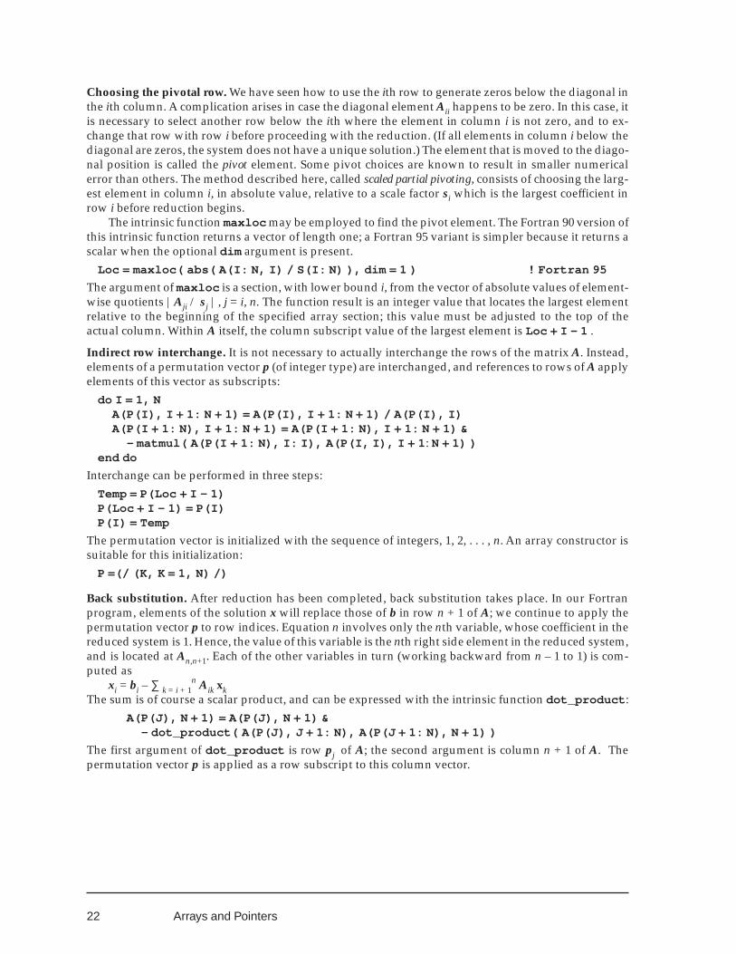
Choosing the pivotal row. We have seen how to use the ith row to generate zeros below the diagonal inthe ith column. A complication arises in case the diagonal element Aii happens to be zero. In this case, itis necessary to select another row below the ith where the element in column i is not zero, and to ex-change that row with row i before proceeding with the reduction. (If all elements in column i below thediagonal are zeros, the system does not have a unique solution.) The element that is moved to the diago-nal position is called the pivot element. Some pivot choices are known to result in smaller numericalerror than others. The method described here, called scaled partial pivoting, consists of choosing the larg-est element in column i, in absolute value, relative to a scale factor si which is the largest coefficient inrow i before reduction begins.
The intrinsic function maxloc may be employed to find the pivot element. The Fortran 90 version ofthis intrinsic function returns a vector of length one; a Fortran 95 variant is simpler because it returns ascalar when the optional dim argument is present.
Loc = maxloc( abs( A(I: N, I) / S(I: N) ), dim = 1 ) ! Fortran 95
The argument of maxloc is a section, with lower bound i, from the vector of absolute values of element-wise quotients |Aji / sj |, j = i, n. The function result is an integer value that locates the largest elementrelative to the beginning of the specified array section; this value must be adjusted to the top of theactual column. Within A itself, the column subscript value of the largest element is Loc + I - 1 .
Indirect row interchange. It is not necessary to actually interchange the rows of the matrix A. Instead,elements of a permutation vector p (of integer type) are interchanged, and references to rows of A applyelements of this vector as subscripts:
do I = 1, NA(P(I), I + 1: N + 1) = A(P(I), I + 1: N + 1) / A(P(I), I)A(P(I + 1: N), I + 1: N + 1) = A(P(I + 1: N), I + 1: N + 1) &
- matmul( A(P(I + 1: N), I: I), A(P(I, I), I + 1: N + 1) )end do
Interchange can be performed in three steps:Temp = P(Loc + I - 1)P(Loc + I - 1) = P(I)P(I) = Temp
The permutation vector is initialized with the sequence of integers, 1, 2, . . . , n. An array constructor issuitable for this initialization:
P =(/ (K, K = 1, N) /)
Back substitution. After reduction has been completed, back substitution takes place. In our Fortranprogram, elements of the solution x will replace those of b in row n + 1 of A; we continue to apply thepermutation vector p to row indices. Equation n involves only the nth variable, whose coefficient in thereduced system is 1. Hence, the value of this variable is the nth right side element in the reduced system,and is located at An,n+1. Each of the other variables in turn (working backward from n – 1 to 1) is com-puted as
xi = bi – ∑ k = i + 1n Aik xk
The sum is of course a scalar product, and can be expressed with the intrinsic function dot_product :A(P(J), N + 1) = A(P(J), N + 1) &
- dot_product( A(P(J), J + 1: N), A(P(J + 1: N), N + 1) )The first argument of dot_product is row pj of A; the second argument is column n + 1 of A. Thepermutation vector p is applied as a row subscript to this column vector.
Arrays and Pointers
23
Say It with Fortran
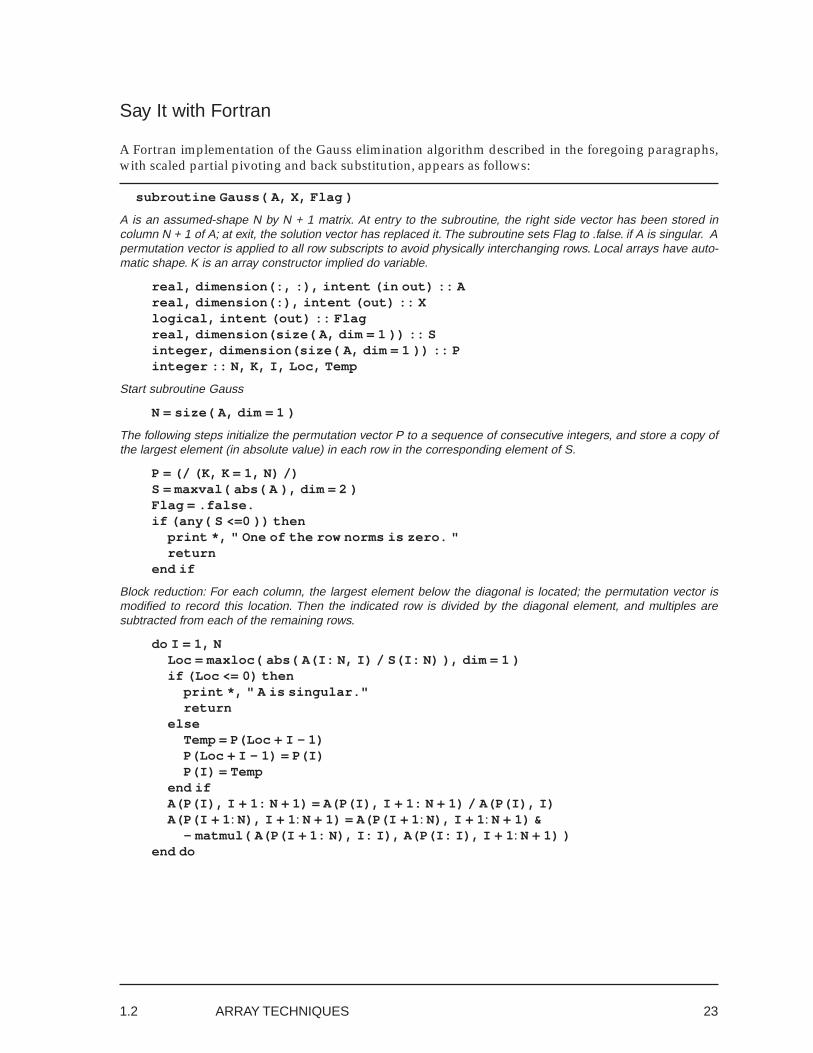
A Fortran implementation of the Gauss elimination algorithm described in the foregoing paragraphs,with scaled partial pivoting and back substitution, appears as follows:
subroutine Gauss( A, X, Flag )
A is an assumed-shape N by N + 1 matrix. At entry to the subroutine, the right side vector has been stored incolumn N + 1 of A; at exit, the solution vector has replaced it. The subroutine sets Flag to .false. if A is singular. Apermutation vector is applied to all row subscripts to avoid physically interchanging rows. Local arrays have auto-matic shape. K is an array constructor implied do variable.
real, dimension(:, :), intent (in out) :: Areal, dimension(:), intent (out) :: Xlogical, intent (out) :: Flagreal, dimension(size( A, dim = 1 )) :: Sinteger, dimension(size( A, dim = 1 )) :: Pinteger :: N, K, I, Loc, Temp
Start subroutine Gauss
N = size( A, dim = 1 )
The following steps initialize the permutation vector P to a sequence of consecutive integers, and store a copy ofthe largest element (in absolute value) in each row in the corresponding element of S.
P = (/ (K, K = 1, N) /)S = maxval( abs( A ), dim = 2 )Flag = .false.if (any( S <=0 )) then
print *, " One of the row norms is zero. "return
end if
Block reduction: For each column, the largest element below the diagonal is located; the permutation vector ismodified to record this location. Then the indicated row is divided by the diagonal element, and multiples aresubtracted from each of the remaining rows.
do I = 1, NLoc = maxloc( abs( A(I: N, I) / S(I: N) ), dim = 1 )if (Loc <= 0) then
print *, " A is singular."return
elseTemp = P(Loc + I - 1)P(Loc + I - 1) = P(I)P(I) = Temp
end ifA(P(I), I + 1: N + 1) = A(P(I), I + 1: N + 1) / A(P(I), I)A(P(I + 1: N), I + 1: N + 1) = A(P(I + 1: N), I + 1: N + 1) &
- matmul( A(P(I + 1: N), I: I), A(P(I: I), I + 1: N + 1) )end do
1.2 ARRAY TECHNIQUES
24
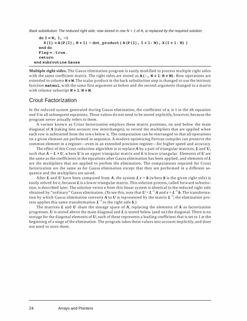
Back substitution: The reduced right side, now stored in row N + 1 of A, is replaced by the required solution.
do I = N, 1, -1X(I) = A(P(I), N + 1) - dot_product( A(P(I), I + 1: N), X(I + 1: N) )
end doFlag = .true.return
end subroutine Gauss
Multiple right sides. The Gauss elimination program is easily modified to process multiple right sideswith the same coefficient matrix. The right sides are stored as A(:, N + 1: N + M). Row operations areextended to column N + M. The scalar product in the back substitution step is changed to use the intrinsicfunction matmul , with the same first argument as before and the second argument changed to a matrixwith column subscript N + 1: N + M.
Crout Factorization
In the reduced system generated during Gauss elimination, the coefficient of xi is 1 in the ith equationand 0 in all subsequent equations. These values do not need to be stored explicitly, however, because theprogram never actually refers to them.
A variant known as Crout factorization employs these matrix positions, on and below the maindiagonal of A (taking into account row interchanges), to record the multipliers that are applied wheneach row is subtracted from the rows below it. The computation can be rearranged so that all operationson a given element are performed in sequence. A modern optimizing Fortran compiler can preserve thecommon element in a register—even in an extended precision register—for higher speed and accuracy.
The effect of this Crout reduction algorithm is to replace A by a pair of triangular matrices, L and U,such that A = L × U, where U is an upper triangular matrix and L is lower triangular. Elements of U arethe same as the coefficients in the equations after Gauss elimination has been applied, and elements of Lare the multipliers that are applied to perfom the elimination. The computations required for Croutfactorization are the same as for Gauss elimination except that they are performed in a different se-quence and the multipliers are saved.
After L and U have been computed from A, the system L c = b (where b is the given right side) iseasily solved for c, because L is a lower triangular matrix. This solution process, called forward substitu-tion, is described later. The solution vector c from this linear system is identical to the reduced right sideobtained by “ordinary” Gauss elimination. (To see this, note that U = L–1 A and c = L–1 b. The transforma-tion by which Gauss elimination converts A to U is represented by the matrix L–1; the elimination pro-cess applies this same transformation L–1 to the right side b.)
The matrices L and U share the storage space of A, replacing the elements of A as factorizationprogresses. U is stored above the main diagonal and L is stored below (and on) the diagonal. There is nostorage for the diagonal elements of U; each of these represents a leading coefficient that is set to 1 at thebeginning of a stage of the elimination. The program takes these values into account implicitly, and doesnot need to store them.
Arrays and Pointers
25
Incorporating row interchanges, the actual factorization can be represented as P A = L U. The per-mutation matrix P is defined by interchanging the rows of an identity matrix in the designated manner.(In the actual program, however, row interchanges are recorded in compact form, as a vector rather thanas a matrix.) The given system A x = b becomes P A x = P b or (after the factorization) L U x = P b. HereP b is simply the permuted version of the given right side vector, which we may call b~. Once L, U, andP have been found by the factorization process, forward substitution is applied to solve the lower trian-gular system L c = b~. As before, back substitution is applied to solve U x = c.
With this method, processing the right side may be postponed until after the factorization is com-pleted, rather than being accomplished concurrently. The factors L and U are stored and row inter-changes are recorded. After the factorization is complete, permutation is applied to the right side. For-ward substitution with L followed by backward substitution with U now gives the solution x.
This postponement of right side processing can be important. Some applications involve severalsystems of equations with the same coefficients but with different right sides. The factorization stepinvolves only the coefficient matrix, and needs to be performed only once. Later, forward and backwardsubstitution can be applied separately to each of the right sides. The number of computation steps re-quired for Crout factorization (done only once) is roughly proportional to n3, while the number of stepsfor forward and back substitution (repeated for each different right side) is proportional to n2. The fol-lowing are two such applications:• For some very common data fitting calculations, A depends upon the characteristics of a measuring
instrument while b is obtained from measured data values. Thus, the factorization can be performedonce and applied to many sets of data over the lifetime of the instrument.
• The process of iterative refinement, which is a simple way to improve the accuracy of the solution ofmany linear algebraic systems and to estimate the validity of the result, is described below. Thisprocess requires solving a related system with the same matrix A and with a new right side that isnot available at the time of the original reduction process, being computed as a high precision re-s i d u a l .Factorization alternates between reducing a column of L (below the diagonal) and a row of U (to the
right of the diagonal). A preliminary Crout factorization program that ignores row interchanges and“unrolls” all array section operations into explicit loops appears as follows:
do I = 1, N! Reduce column Ido J = I, N
do K = 1, I - 1A(J, I) = A(J, I) - A(J, K) * A(K, I)
end doend do! Reduce row Ido J = I + 1, N
do K = 1, I - 1A(I, J) = A(I, J) - A(I, K) * A(K, J)
end doA(I, J) = A(I, J) / A(I, I)
end doend do
1.2 ARRAY TECHNIQUES
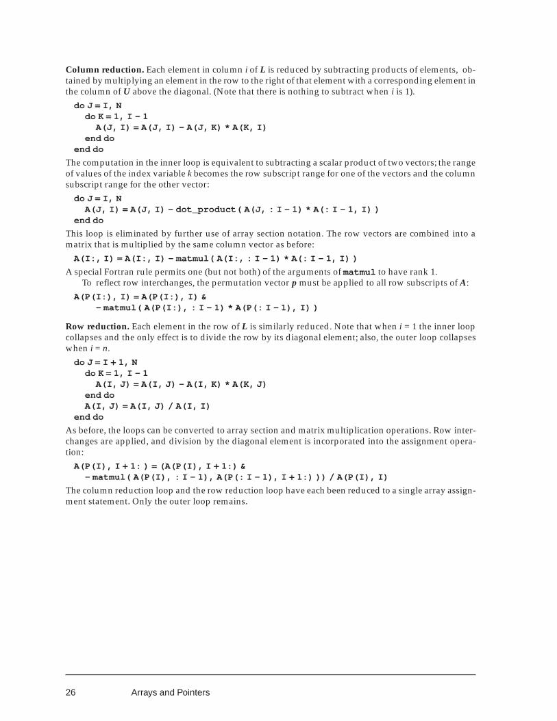
26
Column reduction. Each element in column i of L is reduced by subtracting products of elements, ob-tained by multiplying an element in the row to the right of that element with a corresponding element inthe column of U above the diagonal. (Note that there is nothing to subtract when i is 1).
do J = I, Ndo K = 1, I - 1
A(J, I) = A(J, I) - A(J, K) * A(K, I)end do
end do
The computation in the inner loop is equivalent to subtracting a scalar product of two vectors; the rangeof values of the index variable k becomes the row subscript range for one of the vectors and the columnsubscript range for the other vector:
do J = I, NA(J, I) = A(J, I) - dot_product( A(J, : I - 1) * A(: I - 1, I) )
end do
This loop is eliminated by further use of array section notation. The row vectors are combined into amatrix that is multiplied by the same column vector as before:
A(I:, I) = A(I:, I) - matmul( A(I:, : I - 1) * A(: I - 1, I) )A special Fortran rule permits one (but not both) of the arguments of matmul to have rank 1.
To reflect row interchanges, the permutation vector p must be applied to all row subscripts of A:A(P(I:), I) = A(P(I:), I) &
- matmul( A(P(I:), : I - 1) * A(P(: I - 1), I) )
Row reduction. Each element in the row of L is similarly reduced. Note that when i = 1 the inner loopcollapses and the only effect is to divide the row by its diagonal element; also, the outer loop collapseswhen i = n.
do J = I + 1, Ndo K = 1, I - 1
A(I, J) = A(I, J) - A(I, K) * A(K, J)end doA(I, J) = A(I, J) / A(I, I)
end do
As before, the loops can be converted to array section and matrix multiplication operations. Row inter-changes are applied, and division by the diagonal element is incorporated into the assignment opera-tion:
A(P(I), I + 1: ) = (A(P(I), I + 1:) &- matmul( A(P(I), : I - 1), A(P(: I - 1), I + 1:) )) / A(P(I), I)
The column reduction loop and the row reduction loop have each been reduced to a single array assign-ment statement. Only the outer loop remains.
Arrays and Pointers
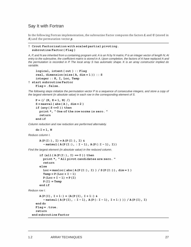
27
Say It with Fortran
In the following Fortran implementation, the subroutine Factor computes the factors L and U (stored inA) and the permutation vector p.
! Crout Factorization with scaled partial pivoting.subroutine Factor( Flag )
A, P, and N are inherited from a containing program unit. A is an N by N matrix; P is an integer vector of length N; Atentry to the subroutine, the coefficient matrix is stored in A. Upon completion, the factors of A have replaced A andthe permutation is recorded in P. The local array S has automatic shape. K is an array constructor implied dovariable.
logical, intent( out ) :: Flagreal, dimension(size( A, dim = 1 )) :: Sinteger :: K, I, Loc, Temp
! start subroutine FactorFlag = .false.
The following steps initialize the permutation vector P to a sequence of consecutive integers, and store a copy ofthe largest element (in absolute value) in each row in the corresponding element of S.
P = (/ (K, K = 1, N) /)S = maxval( abs( A ), dim = 2 )if (any( S <=0 )) then
print *, " One of the row norms is zero. "return
end if
Column reduction and row reduction are performed alternately.
do I = 1, N
Reduce column I.
A(P(I:), I) = A(P(I:), I) &- matmul( A(P(I:), : I - 1), A(P(:I - 1), I))
Find the largest element (in absolute value) in the reduced column.
if (all( A(P(I:), I) == 0 )) thenprint *, " All pivot candidates are zero. "return
elseLoc = maxloc( abs( A(P(I:), I) ) / S(P(I:)), dim = 1 )Temp = P(Loc + I - 1)P(Loc + I - 1) = P(I)P(I) = Temp
end if
Reduce row I.
A(P(I), I + 1:) = (A(P(I), I + 1:) &- matmul( A(P(I), : I - 1), A(P(: I - 1), I + 1:) )) / A(P(I), I)
end doFlag = .true.return
end subroutine Factor
1.2 ARRAY TECHNIQUES
28
A separate subroutine applies the result of Crout factorization to a right side vector. This subroutinecould easily be modified to process multiple right sides. The arguments B and X and the local array Cwould all be changed to n by m matrices; scalar products in the forward and back substitution stepswould be changed to matrix multiplication.
subroutine For_Bak( B, X )
A, P, and N are inherited from a containing program unit. A previous call to Factor has replaced A with its LUfactorization, and has recorded the permutation in P. The vectors B and X have length N.
real, dimension(:), intent( in ) :: Breal, dimension(:), intent( out ) :: Xreal, dimension(N) :: Cinteger :: I
Start subroutine For_Bak
Forward substitution.
do I = 1, NC(I) = (B(P(I)) - dot_product( A(P(I), : I - 1), C(: I - 1) )) / A(P(I), I)
end do
Back substitution.
do I = N, 1, -1X(I) = C(I) - dot_product( A(P(I), I + 1:), X(I + 1:) )
end doreturn
end subroutine For_Bak
Iterative Refinement
Once upon a time, a linear system A x = b was considered difficult if the determinant of its coefficientmatrix A was small. It is now understood that a much more significant criterion is the condition number ofthe coefficient matrix. This number, cond (A), is the product of the norms of A and of its inverse. Multi-plying an n by n matrix by a scalar k has no effect on the condition number, but multiplies the determi-nant by kn. It is possible to obtain a fairly accurate and rather inexpensive estimate of cond (A) as abyproduct of solving the linear system.
Forsythe and Moler (page 20) describe cond (A) as a measure of the maximum distortion that thelinear transformation with matrix A makes on the unit sphere, which is a bound for the ratio of therelative uncertainty of the solution x to that of the given right side b. The value of cond (A) is always 1 orgreater; if its order of magnitude is 10n, the solution can contain approximately n fewer correct signifi-cant decimal digits than the data. Thus, in single precision on typical IEEE hardware the data is repre-sented with about 6 decimals, and a condition number as large as 106 can indicate that the solution isworthless.
Small matrices as “ill conditioned” as this do not appear every day, but they are not extremely rare,either: As an example, the 2 by 2 matrix A with aij = n + i + j, where n is large, has determinant –1 and(depending on the norm) condition number approximately 4n2: The condition number of the matrix
499 500500 501
is about 106.
Arrays and Pointers
29
The accuracy of a computed solution xc can be checked by calculating the residual vector r = b - A xcwhich would be zero if there were no numerical errors. In practice (as Wilkinson discovered early in thedays of computing), any well constructed Gauss elimination or Crout factorization program produces asolution with an acceptably small residual, so practically nothing is learned by simply calculating theresidual. However, solving the system A e = r gives an estimate of (x – xc), the error in x:
r = b – A xc = A x – A xc = A (x – xc)The solution e can be used as an error estimate or can be added to xc to refine the solution. For the latterpurpose, the residual must be calculated with high precision.
If the data is represented with 6 digits and the relative error norm(e) / norm(xc) is 10–2, we say that thesolution contains 4 fewer significant digits than the data, and we may estimate cond(A) as 104. Looselyspeaking, with 6-decimal hardware we might have expected the relative error to be as small as10-6 butwe find it to be 104 times as large as we expect; the factor 104 is attributable to the large conditionnumber. We may add e to xc to obtain a refined solution.
If we iterate this process, we find that the relative error decreases by about the same amount eachtime: in this example, the relative error should be about 10–4 after the first refinement and about 10–6 (asgood as can be obtained with 6-digit arithmetic) after the second. For further details, see Chapter 13 ofthe book by Forsythe and Moler. The electronically distributed examples include program D01C whichapplies the Crout method without iterative refinement, and D01 with refinement. The first set of ex-ample data is an ill-conditioned problem with a known solution; the Crout solution (and the first step ofiterative refinement) contains two or three correct decimal digits; after the third iteration, the solution iscorrect to IEEE hardware precision.
Iterative refinement costs very little (see Exercise 7 below), especially in view of the valuable infor-mation that it provides. As pointed out earlier, most of the computational effort of the Crout method isin the factorization. If the factors are saved, little extra work is required for solving the related systemA e = r. Each step of iterative refinement computes a new residual and applies forward and back substi-tution to obtain a new estimate of the error.
Example 1. The following program performs Crout factorization with partial pivoting, indirectrow interchange, and iterative refinement. It processes multiple right sides, as described earlier. (If thereis only one right side, it must be formatted as an n by 1 array and not as a vector.) Working storageemploys private allocatable arrays at the module level. These remain allocated so that new right sidesmay be processed.
! Example 1. Linear Algebraic Equations by Crout Factorization! with Iterative Refinementmodule D01_M
Specification part
implicit nonepublic :: Solve, Iterateprivate :: Factor, For_Bak, Residualinteger, parameter, private :: HI = kind( 1.0d0 )integer, save, private :: Nreal, dimension(:, :), allocatable, save, private :: LUreal(kind = HI), dimension(:, :), allocatable, save, private :: Save_Ainteger, dimension(:), allocatable, save, private :: Plogical, save, private :: Saved, Exist = .false.integer, private :: I
Procedure part
contains
1.2 ARRAY TECHNIQUES
30
subroutine Solve( A, B, X, Rel_Err, Flag )
This subroutine solves the system of simultaneous linear algebraic equations A X = B, where A is an N by N matrixand X and B are N by M matrices. A and B are assumed-shape arrays supplied by the calling program. X, Rel_Err,and Flag are computed and returned by Factor. Solve does not change A or B. On return from Solve, X contains thesolution and Rel_Err contains an estimate of the relative error in X. However, if Flag is false, the contents of X andRel_Err are unpredictable, since the algorithm has short-circuited. The problem size N, a copy of A, and the LUdecomposition matrix (with permutation vector P) are saved as private module-level variables, and are not changedexcept when Solve is called.
DUMMY ARGUMENTS and LOCAL DATA (K is an array constructor implied do variable.)
real, dimension(:, :), intent (in) :: A, Breal, dimension(:, :), intent (out) :: Xreal, intent (out) :: Rel_Errlogical, intent (out) :: Flaginteger :: K
Start subroutine Solve. Determine problem size; initialize private arrays
Saved = .false.Flag = .false.N = size( A, dim = 1 )if (size( A, dim = 2 ) /= N &
.or. size( B, dim = 1 ) /= N &
.or. any( shape( X ) /= shape( B ) )) thenprint *, " SOLVE argument shape incompatibility."return
end if
Allocate working arrays. Exist is a logical variable at the module level that is true when the necessary arrays havebeen allocated. Save a high-precision copy of A (without row interchanges) for the residual calculation. Store rownorms in S.
if (Exist) deallocate( Save_A, LU, P )if (N == 0) then
Exist = .false.return
end ifallocate( Save_A(N, N), LU(N, N), P(N) )Exist = .true.Save_A = real( A, kind = HI )LU = AP = (/ (K, K = 1, N) /)call Factor( )
Saved is a logical variable at the module level that is true when a Crout factorization has been performed and thenecessary arrays have been saved so that a solution can be calculated from any given right side.
if (Flag) thenSaved = .true.call For_Bak( B, X )call Iterate ( B, X, Rel_Err )if (Rel_Err > 0.5 )) then
print *, " Relative Error > 0.5.", Rel_ErrFlag = .false.
end ifend ifreturn
Arrays and Pointers
31
contains
Internal procedure to perform factorization A = L * U with scaled partial pivoting. Column reduction and row reduc-tion are performed alternately.
subroutine Factor( )
LOCAL DATA
real, dimension(N) :: Sinteger :: I, Loc, Temp
Start subroutine Factor
Flag = .false.S = maxval( abs( LU ), dim = 2 )if (any( S <= 0 )) then
print *, " Row norms: ", Sprint *, " One of the row norms is zero. "return
end ifdo I = 1, N
Reduce column I.
LU(P(I:), I) = LU(P(I:), I) &- matmul( LU(P(I:), : I - 1), LU(P(:I - 1), I) )
Find the largest element (in absolute value) in the reduced column; record row interchange in P.
if (all( LU(P(I:), I) == 0 )) thenprint *, " All pivot candidates are zero. "return
elseLoc = maxloc( abs( LU(P(I:), I) ) / S(P(I:)), dim = 1 ) + I - 1Temp = P(Loc)P(Loc) = P(I)P(I) = Temp
end if
Reduce row I.
LU(P(I), I + 1:) = (LU(P(I), I + 1:) &- matmul( LU(P(I), : I - 1), LU(P(: I - 1), I + 1:) )) &/ LU(P(I), I)
end do
Flag = .true.return
end subroutine Factor
end subroutine Solve
1.2 ARRAY TECHNIQUES
32
subroutine Iterate (B, X, Rel_Err)
DUMMY ARGUMENTS and LOCAL DATA
real, dimension(:, :), intent (in) :: Breal, dimension(:, :), intent (out) :: Xreal, intent (out) :: Rel_Errreal, dimension(size( B, dim = 1 ), size( B, dim = 2 )) :: R, E
Start subroutine Iterate
if (.not. Saved &.or. size( B, dim = 1 ) /= N &.or. any( shape( X ) /= shape( B ) )) thenprint *, " ITERATE argument shape incompatibility."return
end if
Calculate high-precision residual for right side B and solution X, using Save_A from latest call to Factor. For eachright side column, calculate norm of the residual; find largest such norm among all right sides.
R = real( real( B, kind = HI ) - matmul( Save_A, real( X, kind = HI ) ) )print *, " Residual: ", maxval( sqrt( sum( R ** 2, dim = 1 ) ) )
Use the calculated residual to “refine” X. For each right side, divide norm of the error estimate by norm of thesolution; find largest such ratio among all right sides. Reference to tiny guarantees no division by zero.
call For_Bak( R, E )X = X + ERel_Err = maxval( sqrt( sum( E ** 2, dim = 1 ) ) &
/ max( sqrt( sum( X ** 2, dim = 1 ) ), 8 * tiny( 1.0 ) ) )return
end subroutine Iterate
The subroutine For_Bak performs forward and back substitution, using LU and P stored at the latest call to Factor.B is M right side vectors. The result will be returned in X.
subroutine For_Bak( B, X )
DUMMY ARGUMENTS and LOCAL DATA
real, dimension(:, :), intent (in) :: Breal, dimension(:, :), intent (out) :: Xinteger :: Ireal, dimension(size( B, dim = 1), size( B, dim = 2)) :: C
Start subroutine For_Bak
do I = 1, NC(I, :) = (B(P(I), :) &
- matmul( LU(P(I), : I - 1), C(: I - 1, :) )) / LU(P(I), I)end dodo I = N, 1, -1
X(I, :) = C(I, :) - matmul( LU(P(I), I + 1: ), X(I + 1: , :) )end doreturn
end subroutine For_Bak
end module D01_M
Arrays and Pointers
33
As in the following test driver, the main program must provide space for data arrays A and B as wellas for the result array X. Here, these are allocated after the array size has been read. A call to Solvecomputes an approximate solution and performs one step of iterative refinement to estimate the relativeerror. The program calls Iterate as necessary to reduce the relative error to an acceptable value. Fi-nally, the arrays allocated at the main program level are deallocated.
program D01
Example driver program for Crout factorization with iterative refinement.
use D01_Mimplicit noneinteger :: EoF, I, M, N, Loopreal, dimension(:, :), allocatable :: A, B, Xreal :: Rel_Errlogical :: Flag
Start program. Connect input file and read N, the number of equations, from the first record.
open (unit = 1, file = "gaudata.txt", &status = "old", action = "read", position = "rewind")
read (unit = 1, fmt = *, iostat = EoF) Nif (EoF /= 0) then
print *, " Data error at start of file. "end if
Allocate A and read values for A, by rows. Echo print A.
allocate( A(N, N) )do I = 1, N
read (unit = 1, fmt = *) A(I, :)if (EoF /= 0) then
print *, " Insufficient data for A. "end ifprint *, " Matrix A, Row ", I, A(I, :)
end do
Read M, the number of right sides. Allocate arrays for B and for results. Read B by rows and echo print it.
read (unit = 1, fmt = *, iostat = EoF) Mif (EoF /= 0) then
print *, " Insufficient data for M. "end ifallocate( B(N, M), X(N, M) )do I = 1, N
read (unit = 1, fmt = *) B(I, :)if (EoF /= 0) then
print *, " Insufficient data for B. "end ifprint *, " Matrix B, Row ", I, B(I, :)
end do
1.2 ARRAY TECHNIQUES
34
Solve for X in A X = B. Print initial error estimate.
call Solve( A, B, X, Rel_Err, Flag )if (.not. Flag) then
print *, " Factor cannot solve this one."stop
elseprint *, 0, " Relative error: ", Rel_Err
end if
(Optional) Iterative refinement. Stop when relative error is small or after 10 iterations; print the relative error esti-mate for each iteration.
do Loop = 1, 10if (Rel_Err < 1.0e-7) exitcall Iterate(B, X, Rel_Err)print *, Loop, " Relative error: ", Rel_Err
end do
Print the final result.
do I = 1, Mprint *, " Matrix X, Column ", I, X(:, I)
end dostop
end program D01
Another driver is distributed electronically as example D01X. This driver generates a rather largeill-conditioned matrix, inverts it, and then re-inverts the inverse; the driver also estimates the time re-quired for the computation.
Section 1.2 Exercises1. If the next student is taller than the one standing by the door, you ask the next student to stand there
instead. If the next student is not taller, you leave the previous student standing there. Explain howthis repeated step preserves the invariant assertion, “The tallest student in the dining hall is nowstanding at the left of the doorway.”
2. For the function Minimum_Location , show that executing an iteration of the loop preserves theinvariant assertion.
a) Is the procedure correct when Loc_1 and Loc_2 have the same value?
b) Does the procedure work correctly for an array of size zero (e.g., when Loc_1 is 1 and Loc_2 iszero)? If not, what changes should be made?
3. For the function Linear_Search , show that executing an iteration of the loop preserves the invari-ant assertion.
a) If the procedure terminates because the key matches an array element, show that the assertion istrue.
b) Show that the invariant assertion is always preserved during every iteration of the loop.
c) In case the loop exit is taken, the invariant assertion is true and 1 ≤ i ≤ N. Show that the key valuelies between Arrayi–1 and Arrayi even if i is 1.
d) In case the loop exit is not taken, the invariant assertion is true and the value of i is N + 1. Showthat the key value lies between Arrayi–1 and Arrayi .
e) What will happen if the given array has zero length (i.e., if size( Array ) is zero)?
Arrays and Pointers
351.2 ARRAY TECHNIQUES
4. Study the function Binary_Search .
a) Show that Middle is always between 1 and N inclusive: i.e., Array(Middle) is always anelement within the designated array section and is never one of the fictitious elements Array(0)or Array(N + 1).
b) Show that the integer division step preserves the relation Loc_1 ≤ Middle ≤ Loc_2.
c) Show that if Loc_1 and Loc_2 differ by exactly two at the beginning of an iteration, they differby exactly one at the end of the same iteration. (Consider all possible combinations of odd andeven values.)
d) Show that the invariant assertion is always preserved during every iteration of the loop; showthat it would still be preserved without the exact match shortcut.
e) In case the key matches an array element, at loop termination the invariant assertion is true andthe while condition is also true. Since the key cannot match a fictitious element, Loc_1 is atleast 1 and Loc_2 is at most N. Show that the key value lies between Array(Loc_1) andArray(Loc_2) .
f) In case the key does not match any Array element, at loop termination the invariant assertion istrue and the while condition is false. Show that the key value lies between Array(Loc_1)and Array(Loc_2) , even if Loc_1 is zero or Loc_2 is N + 1.
g) What happens when the given array has one element? Consider the case in which the key matchesthe array element, as well as the case in which it does not match.
h) What happens when the size of the given array is zero?
5. Rewrite Binary_Search to use recursion instead of iteration.
6. The three-way comparison in Binary_Search is more efficient than a simple two-way compari-son if the search key actually appears in the array. Quantify the expected improvement in terms of p,the probability that the key is present in the array.
7. For the Crout algorithm with iterative refinement, matrix factorization requires on the order of n3
operations. Forward substitution, back substitution, and calclulating the residual each require onthe order of n2 operations. Give arguments to support the following conjectures.
a) If n ≥ 10, the amount of computation required for iterative refinement is insignificant.
b) If n < 10, the amount of computation required for iterative refinement is insignificant.
Compare B.W. Kernighan and P.J. Plauger, “The Elements of Programming Style” (McGraw-Hill,1974), p. 9.
8. Run the program of Example 1 with the electronically distributed file gaudata.txt , and estimatethe condition number of each (nonsingular) matrix in the data set.
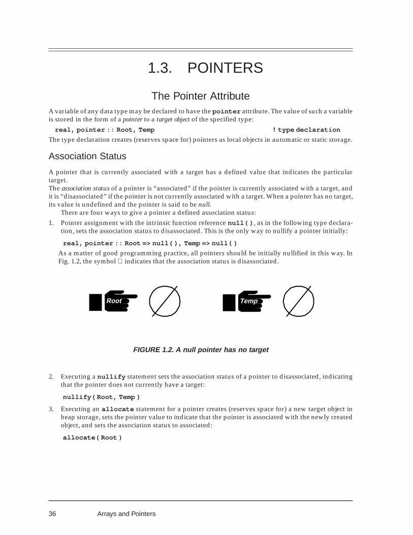
36
Root Temp
1.3. POINTERS
The Pointer AttributeA variable of any data type may be declared to have the pointer attribute. The value of such a variableis stored in the form of a pointer to a target object of the specified type:
real, pointer :: Root, Temp ! type declaration
The type declaration creates (reserves space for) pointers as local objects in automatic or static storage.
Association Status
A pointer that is currently associated with a target has a defined value that indicates the particulartarget.The association status of a pointer is “associated” if the pointer is currently associated with a target, andit is “disassociated” if the pointer is not currently associated with a target. When a pointer has no target,its value is undefined and the pointer is said to be null.
There are four ways to give a pointer a defined association status:1. Pointer assignment with the intrinsic function reference null( ) , as in the following type declara-
tion, sets the association status to disassociated. This is the only way to nullify a pointer initially:
real, pointer :: Root => null( ), Temp => null( )As a matter of good programming practice, all pointers should be initially nullified in this way. InFig. 1.2, the symbol ∅ indicates that the association status is disassociated.
FIGURE 1.2. A null pointer has no target
2. Executing a nullify statement sets the association status of a pointer to disassociated, indicatingthat the pointer does not currently have a target:
nullify( Root, Temp )
3. Executing an allocate statement for a pointer creates (reserves space for) a new target object inheap storage, sets the pointer value to indicate that the pointer is associated with the newly createdobject, and sets the association status to associated:
allocate( Root )
Arrays and Pointers
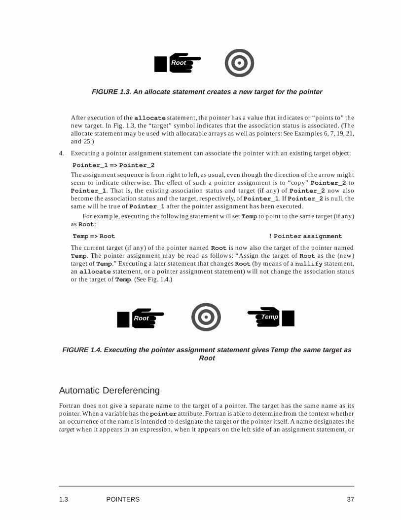
37
FIGURE 1.3. An allocate statement creates a new target for the pointer
After execution of the allocate statement, the pointer has a value that indicates or “points to” thenew target. In Fig. 1.3, the “target” symbol indicates that the association status is associated. (Theallocate statement may be used with allocatable arrays as well as pointers: See Examples 6, 7, 19, 21,and 25.)
4. Executing a pointer assignment statement can associate the pointer with an existing target object:
Pointer_1 => Pointer_2
The assignment sequence is from right to left, as usual, even though the direction of the arrow mightseem to indicate otherwise. The effect of such a pointer assignment is to “copy” Pointer_2 toPointer_1 . That is, the existing association status and target (if any) of Pointer_2 now alsobecome the association status and the target, respectively, of Pointer_1 . If Pointer_2 is null, thesame will be true of Pointer_1 after the pointer assignment has been executed.
For example, executing the following statement will set Temp to point to the same target (if any)as Root :
Temp => Root ! Pointer assignment
The current target (if any) of the pointer named Root is now also the target of the pointer namedTemp. The pointer assignment may be read as follows: “Assign the target of Root as the (new)target of Temp.” Executing a later statement that changes Root (by means of a nullify statement,an allocate statement, or a pointer assignment statement) will not change the association statusor the target of Temp. (See Fig. 1.4.)
1.3 POINTERS
FIGURE 1.4. Executing the pointer assignment statement gives Temp the same target asRoot
Automatic Dereferencing
Fortran does not give a separate name to the target of a pointer. The target has the same name as itspointer. When a variable has the pointer attribute, Fortran is able to determine from the context whetheran occurrence of the name is intended to designate the target or the pointer itself. A name designates thetarget when it appears in an expression, when it appears on the left side of an assignment statement, or
Root
Root Temp
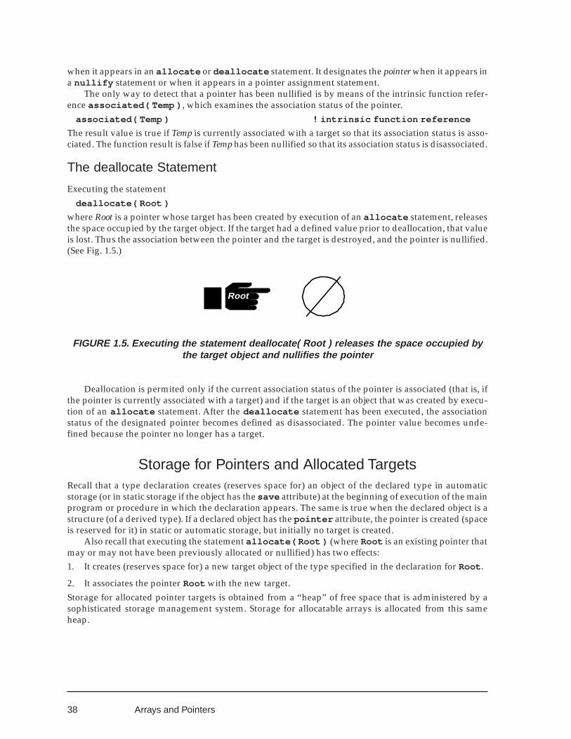
38
when it appears in an allocate or deallocate statement. It designates the pointer when it appears ina nullify statement or when it appears in a pointer assignment statement.
The only way to detect that a pointer has been nullified is by means of the intrinsic function refer-ence associated( Temp ) , which examines the association status of the pointer.
associated( Temp ) ! intrinsic function reference
The result value is true if Temp is currently associated with a target so that its association status is asso-ciated. The function result is false if Temp has been nullified so that its association status is disassociated.
The deallocate Statement
Executing the statementdeallocate( Root )
where Root is a pointer whose target has been created by execution of an allocate statement, releasesthe space occupied by the target object. If the target had a defined value prior to deallocation, that valueis lost. Thus the association between the pointer and the target is destroyed, and the pointer is nullified.(See Fig. 1.5.)
Arrays and Pointers
Root
FIGURE 1.5. Executing the statement deallocate( Root ) releases the space occupied bythe target object and nullifies the pointer
Deallocation is permited only if the current association status of the pointer is associated (that is, ifthe pointer is currently associated with a target) and if the target is an object that was created by execu-tion of an allocate statement. After the deallocate statement has been executed, the associationstatus of the designated pointer becomes defined as disassociated. The pointer value becomes unde-fined because the pointer no longer has a target.
Storage for Pointers and Allocated TargetsRecall that a type declaration creates (reserves space for) an object of the declared type in automaticstorage (or in static storage if the object has the save attribute) at the beginning of execution of the mainprogram or procedure in which the declaration appears. The same is true when the declared object is astructure (of a derived type). If a declared object has the pointer attribute, the pointer is created (spaceis reserved for it) in static or automatic storage, but initially no target is created.
Also recall that executing the statement allocate( Root ) (where Root is an existing pointer thatmay or may not have been previously allocated or nullified) has two effects:1. It creates (reserves space for) a new target object of the type specified in the declaration for Root .
2. It associates the pointer Root with the new target.Storage for allocated pointer targets is obtained from a “heap” of free space that is administered by asophisticated storage management system. Storage for allocatable arrays is allocated from this sameheap.
39
Management of Allocated Targets
Executing an allocate statement for a pointer causes space from the heap to be reserved for the target,and gives the pointer a value that permits Fortran to gain access to the target via the pointer. At thispoint, Fortran has no other way of obtaining access to the target — that is, to the area of heap space thathas just been allocated.
Some care is required here to avoid storage management problems. If the pointer value is destroyed(by nullification, reallocation, or pointer assignment) but the target is not deallocated, the heap spacebecomes “garbage” — that is, it is still reserved by the storage management system but it is inaccessibleto the program for which it was reserved. To ensure that the target space will be returned to the heap forpossible further use when the pointer is nullified, a deallocate statement should be employed.
After a pointer assignment with a pointer on the right is executed, on the other hand, there is morethan one pointer with the same target. So long as at least one of these pointers remains associated withthe target, the others may be nullified.
But another problem can arise in this case. When two or more pointers have the same target,deallocating one of the pointers deletes the target object (and releases heap storage space) without af-fecting the other pointers. The other pointers are now said to be “dangling references” — pointers toheap space that is no longer reserved.
Programs that manipulate pointers should strictly observe the following important rules:1. If there is only one pointer currently pointing to a particular target object, do not change the value of
(nullify , reallocate, or assign to) the pointer without first deallocating it.
2. If there is more than one pointer currently pointing to a particular target object, do not deallocate anyof these pointers.Some processors provide little assistance for diagnosing allocation errors such as heap overflow.
Fortran provides a second (optional) clause in the allocate statement, of the form stat = Statusvariable. During execution, the Status variable will be set to zero if the allocation is successful, or to apositive value in case of an allocation error such as insufficient heap storage space:
allocate( Temp_NP, stat = Err )if (Err > 0 ) then
:
Pointers as Derived Type ComponentsA component of a derived type may have the pointer attribute. Note the following points:• The type specified for each component in a derived type definition, except for components that have
the pointer attribute, must be an intrinsic type or a previously defined derived type.
• A derived type may have a component that is a pointer to the same type. Such components mostfrequently occur in derived types that are intended for linked list applications.
• Initial nullification may be specified for pointer components. (This feature was introduced in For-tran 95 and is not available with Fortran 90. See the electronically distributed examples for alterna-tive programming strategies.)
• Any pointer component that has the dimension attribute must have deferred shape — its actualsubscript bounds are specified when the target array is allocated rather than in the type definition.
1.3 POINTERS
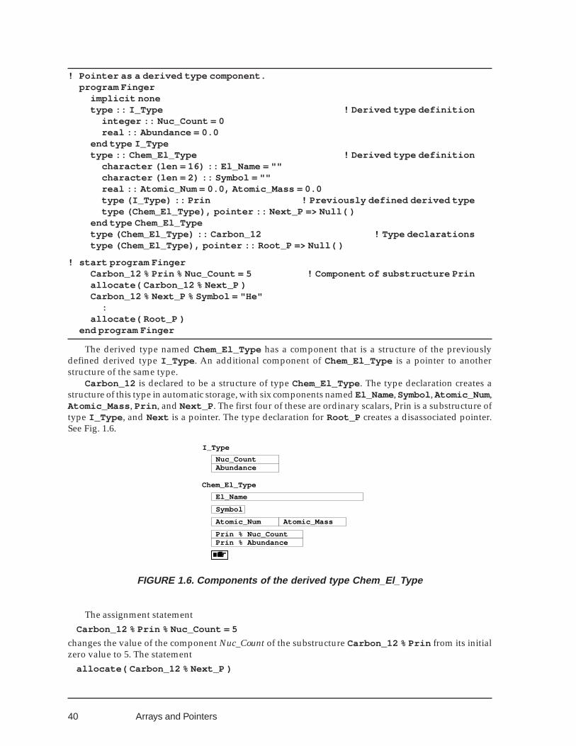
40
Nuc_Count Abundance
I_Type
El_Name
Symbol
Atomic_Num Atomic_Mass
Prin % Nuc_Count Prin % Abundance
Chem_El_Type
! Pointer as a derived type component.program Finger
implicit nonetype :: I_Type ! Derived type definition
integer :: Nuc_Count = 0real :: Abundance = 0.0
end type I_Typetype :: Chem_El_Type ! Derived type definition
character (len = 16) :: El_Name = ""character (len = 2) :: Symbol = ""real :: Atomic_Num = 0.0, Atomic_Mass = 0.0type (I_Type) :: Prin ! Previously defined derived typetype (Chem_El_Type), pointer :: Next_P => Null( )
end type Chem_El_Typetype (Chem_El_Type) :: Carbon_12 ! Type declarationstype (Chem_El_Type), pointer :: Root_P => Null( )
! start program FingerCarbon_12 % Prin % Nuc_Count = 5 ! Component of substructure Prinallocate( Carbon_12 % Next_P )Carbon_12 % Next_P % Symbol = "He"
:allocate( Root_P )
end program Finger
The derived type named Chem_El_Type has a component that is a structure of the previouslydefined derived type I_Type . An additional component of Chem_El_Type is a pointer to anotherstructure of the same type.
Carbon_12 is declared to be a structure of type Chem_El_Type . The type declaration creates astructure of this type in automatic storage, with six components named El_Name, Symbol , Atomic_Num ,Atomic_Mass , Prin , and Next_P . The first four of these are ordinary scalars, Prin is a substructure oftype I_Type , and Next is a pointer. The type declaration for Root_P creates a disassociated pointer.See Fig. 1.6.
Arrays and Pointers
FIGURE 1.6. Components of the derived type Chem_El_Type
The assignment statementCarbon_12 % Prin % Nuc_Count = 5
changes the value of the component Nuc_Count of the substructure Carbon_12 % Prin from its initialzero value to 5. The statement
allocate( Carbon_12 % Next_P )
41
creates a target structure named Carbon_12 % Next_P in heap storage. The assignment statementCarbon_12 % Next_P % Symbol = "He"
assigns the string "He" to the component Symbol in the structure Carbon_12 % Next.Note carefully the difference between two deceptively similar assignment statements.
type :: I_Type ! Derived type definitioninteger :: Nuc_Count = 0real :: Abundance = 0.0
end type I_Typetype :: Chem_El_Type ! Derived type definition
character (len = 16) :: El_Name = ""character (len = 2) :: Symbol = ""real :: Atomic_Num = 0.0, Atomic_Mass = 0.0type (I_Type) :: Prin ! Previously defined derived typetype (Chem_El_Type), pointer :: Next_P => Null( )
end type Chem_El_Typetype (Chem_El_Type) :: Carbon_12 ! Type declarations
:Carbon_12 % Prin % Nuc_Count = 5Carbon_12 % Next_P % Symbol = "He"
The variable name Carbon_12 % Prin % Nuc_Count consists of the name of a declared (automaticstorage) structure, the name of a substructure, and the name of a component of the substructure. On theother hand, in the reference to the variable Carbon_12 % Next_P % Symbol , the component namedNext_P has the pointer attribute, so Carbon_12 % Next_P refers to the structure (in heap storage)that is the target of the pointer, and Symbol is a component of that target structure.
A pointer variable can be created in automatic storage as an independent object that is not part of astructure. The type declaration creates Root_P as a pointer to type Chem_El_Type . Executing the al-locate statement creates a structure named Root_P .
Pointers with ArraysFortran does not provide arrays of pointers. (A variable with pointer and dimension attributes is apointer to an array, not an array of pointers.) However, it is possible to define a structure with a singlecomponent that is a pointer, and then to create an array of these structures. This feature is illustrated inExamples 24 and 25 (in Chapter 7).
1.3 POINTERS
42
Chapter 2 Introduction to Sorting
Your mail has just arrived. Your bank has sent you a statement with last month’s cancelled checks en-closed. There are only three checks, which need to be arranged in numerical order and stored away forfuture reference.
You don’t have to undertake an elaborate research project to decide how to put three checks in order.Here is a simple method:1. Lay the three checks down side by side. Compare the checks that are in the first and second posi-
tions, and interchange them if they are in the wrong order.
2. Compare the checks that are now in the first and third positions, and interchange them if they are inthe wrong order.
3. Compare the checks that are now in the second and third positions, and interchange them if they arein the wrong order.The comparison depends on a sort key. Here we assume that the key is a check number that appears
on each check. (The sort key might instead be the date or the amount.) Objects can be sorted into eitherincreasing or decreasing order, depending upon how the comparison is made. At first, it will be as-sumed that all of the objects have different key values. Duplicate keys cause no real difficulty, but theyintroduce some minor complications that will be considered later in this chapter.
Computer SortingMany computer applications, from maintaining and updating simple arrays to data base indexing,
require sorting of data. It may be that the elements are simply numbers or character strings to be ar-ranged by numerical value, or they may be structures that can be viewed as rows of a table. For example,the table of California cities mentioned earlier might be sorted with respect to any of three keys: alpha-betically by the name of the city, or numerically by latitude or by longitude.
Inside the computer, data to be sorted is usually stored in an array. The sorting procedure convertsan array of unsorted elements into an array of sorted elements. For most applications, large quantities ofextra space are not available — a sorting method that requires as much additional space as the array tobe sorted would usually be considered unacceptable. The sorted data should end up in the same arrayoriginally occupied by the unsorted data.10 Initially, the unsorted data occupies the entire array, andthere is no sorted data.
For example, numbers to be sorted by the three-item sorting method just considered would be storedin an array of length three:
10 This is not true of certain methods such as merge sort that are used mainly for sorting data from external files.
43
subroutine Sort_3( Array )real, intent(in), dimension(3) :: Array
! start subroutine Sort_3if (Array(1) > Array(2)) call Swap( 1, 2 )if (Array(1) > Array(3)) call Swap( 1, 3 )if (Array(2) > Array(3)) call Swap( 2, 3 )return
end subroutine Sort_3
Some computer sorting methods are simple and easy to understand and are adequate for sorting afew (up to perhaps 10,000) data items. As we shall see, these simple methods are impossibly inefficientfor large quantities of data.• Selection sorting is probably the easiest of all known methods to understand and to implement.
• Insertion sorting is faster than selection for “random” data, and is only slightly more complicated.Some variations can considerably increase the speed of this method.The remainder of this chapter is devoted to sorting by the two simplest methods, selection and
insertion.11 Two more sophisticated methods that are related to insertion, Shell sort and heapsort, arealso described here. Quicksort, a method that is usually implemented recursively, is discussed in Chap-ter 3.
Operation Counts for Sort_3
if (Array(I) > Array(J)) call Swap( 1, 2 ) ! 1if (Array(I) > Array(K)) call Swap( 1, 3 ) ! 2if (Array(J) > Array(K)) call Swap( 2, 3 ) ! 3
There are six possibilities, which are equally likely for random data.A B CA C B →→→→→ A B CB A C →→→→→ A B CB C A →→→→→ A C B →→→→→ A B CC A B →→→→→ A C B →→→→→ A B CC B A →→→→→ B C A →→→→→ A C B →→→→→ A B C
The first of these situations requires no swaps, the next two require one swap, the next two require twoswaps, and the last one requires three swaps. Thus the expected number of calls to Swap for randomdata is 1.5. Each call to Swap performs three move operations. The subroutine therefore requires 3 com-parisons and 4.5 moves (for random data). In practice, however, these basic operations are completelydominated by procedure call overhead.
11 Another well-known simple method, bubble sorting, is not discussed in this text.“The bubble sort seems tohave nothing to recommend it, except a catchy name and the fact that it leads to some interesting theoreticalproblems”: Knuth, Sorting and Searching, 111. “If you know what bubble sort is, wipe it from your mind; if youdon’t know, make a point of never finding out!”: Press, et al, Numerical Recipes in Fortran, Second Ed. (Cam-bridge: Cambridge Univ. Press, 1992), 321.
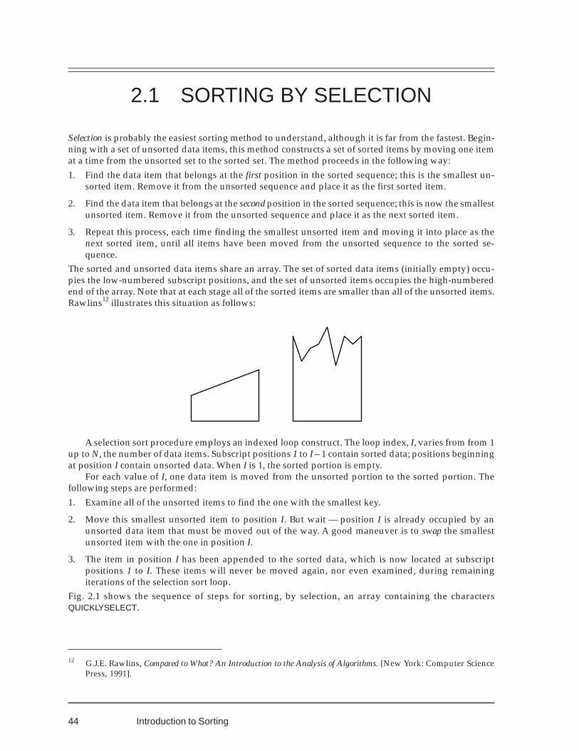
44
2.1 SORTING BY SELECTION
Selection is probably the easiest sorting method to understand, although it is far from the fastest. Begin-ning with a set of unsorted data items, this method constructs a set of sorted items by moving one itemat a time from the unsorted set to the sorted set. The method proceeds in the following way:1. Find the data item that belongs at the first position in the sorted sequence; this is the smallest un-
sorted item. Remove it from the unsorted sequence and place it as the first sorted item.
2. Find the data item that belongs at the second position in the sorted sequence; this is now the smallestunsorted item. Remove it from the unsorted sequence and place it as the next sorted item.
3. Repeat this process, each time finding the smallest unsorted item and moving it into place as thenext sorted item, until all items have been moved from the unsorted sequence to the sorted se-quence.
The sorted and unsorted data items share an array. The set of sorted data items (initially empty) occu-pies the low-numbered subscript positions, and the set of unsorted items occupies the high-numberedend of the array. Note that at each stage all of the sorted items are smaller than all of the unsorted items.Rawlins12 illustrates this situation as follows:
12 G.J.E. Rawlins, Compared to What? An Introduction to the Analysis of Algorithms. [New York: Computer SciencePress, 1991].
A selection sort procedure employs an indexed loop construct. The loop index, I, varies from from 1up to N, the number of data items. Subscript positions 1 to I – 1 contain sorted data; positions beginningat position I contain unsorted data. When I is 1, the sorted portion is empty.
For each value of I, one data item is moved from the unsorted portion to the sorted portion. Thefollowing steps are performed:1. Examine all of the unsorted items to find the one with the smallest key.
2. Move this smallest unsorted item to position I. But wait — position I is already occupied by anunsorted data item that must be moved out of the way. A good maneuver is to swap the smallestunsorted item with the one in position I.
3. The item in position I has been appended to the sorted data, which is now located at subscriptpositions 1 to I. These items will never be moved again, nor even examined, during remainingiterations of the selection sort loop.
Fig. 2.1 shows the sequence of steps for sorting, by selection, an array containing the charactersQUICKLYSELECT.
Introduction to Sorting
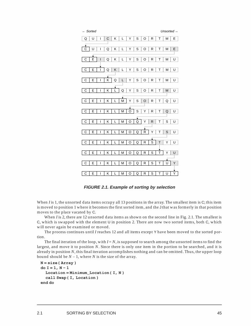
45
FIGURE 2.1. Example of sorting by selection
When I is 1, the unsorted data items occupy all 13 positions in the array. The smallest item is C; this itemis moved to position 1 where it becomes the first sorted item, and the J that was formerly in that positionmoves to the place vacated by C.
When I is 2, there are 12 unsorted data items as shown on the second line in Fig. 2.1. The smallest isC, which is swapped with the element U in position 2. There are now two sorted items, both C, whichwill never again be examined or moved.
The process continues until I reaches 12 and all items except Y have been moved to the sorted por-tion.
The final iteration of the loop, with I = N, is supposed to search among the unsorted items to find thelargest, and move it to position N. Since there is only one item in the portion to be searched, and it isalready in position N, this final iteration accomplishes nothing and can be omitted. Thus, the upper loopbound should be N – 1, where N is the size of the array.
N = size( Array )do I = 1, N - 1
Location = Minimum_Location( I, N )call Swap( I, Location )
end do
2.1 SORTING BY SELECTION
← Sorted Unsorted →
LKCIQ EMTROU SY
C
USTRY
USTYMLKIC ROE Q
UYTMLKIC SROE Q
UYMLKIC TSROE Q
YMLKIC UTSROE Q
MLKIC YUTSROE Q
MLKIC OE Q
LKQI EMTROYU S
LKQI UMTROY SC E
LKQ UMTROY SIC E
LQ UMTROY SKIC E
Q UMTROY SLKIC E
UQTROY SLKIC E M
UQTRYSMLKIC E O
46
The function Minimum_Location is implemented as an internal procedure that inherits Array fromthe host program, so only the two subcript bounds are passed as arguments. The subroutine Swap alsoinherits Array; subscript values for the items to be exchanged are passed as dummy arguments.
Operation Counts for Selection Sort
N = size( Array ) ! 1do I = 1, N - 1 ! 2
Location = Minimum_Location( I, N ) ! < 3call Swap( I, Location ) ! < 4
end do ! < 5Each Swap call requires 3 move operations, as stated earlier. For random data, each reference to the
function Minimum_Location( I, N ) requires N – I + 1 comparisons and 0.7·lg (N – I) + 0.6 moves.Thus, the loop body (lines 3 and 4) performs N – I + 1 comparisons and 4.6 + 0.7·lg (N – I) moves. Theseformulas are to be summed over all N – 1 iterations of the loop.• Terms independent of I are multiplied by N – 1:
N + 1 comparisons times N – 1 = N2 – 1; 4.6 moves times N – 1 = 4.6·N – 4.6
• Terms in I:Sum of – I comparisons for I = 1 to (N – 1) is – 0.5·N2 + 0.5·N
• Terms logarithmic in I:A sum of logarithmic terms can be estimated by analogy to the integral ∫ln z = z(ln z – 1); noting that lg k is about 1.4 ln k, the sum from a to b of lg k is approximately
b lg b – a lg a – 1.4 (b – a).Let k = N – I; the loop is executed with k = N – 1 to 1 so the sum is
(N – 1) lg( N – 1 ) – 1·lg 1 – 1.4 (N – 2)Total comparisons: 0.5·N2 + 0.5·N – 1
Total moves: 0.7·N lg( N – 1 ) + 5.6·N – 0.7·lg( N – 1 ) – 6.6A benchmark, run with a 50 MHz 486DX computer, sorted 20,000 random real numbers by selection
in 350 seconds.
Say It with Fortran
Example 2. This version sorts an array of strings. The subroutine Se_Sort contains two internalprocedures, the function Minimum_Location and the subroutine Swap. The subroutine Se_Sort iscontained in the module D02_M along with a subroutine to print the aray. A main program to test themodule is shown as well.
! Example 2. Sorting an array of strings by selection.module D02_M
implicit nonepublic :: Se_Sort
contains
subroutine Se_Sort( Array ) ! Module subprogram
The dummy argument Array has assumed shape (with rank 1), character type, and assumed length. (The arraysize and the length of the strings in the array will be taken from the actual argument.) Its intent attribute is inout , which means that the corresponding actual argument array must be definable (for example, it must not be anarray-valued expression that contains operators). Its elements must be defined before they are used: here it isassumed that they have defined values at entry to the subroutine.
character (len = *), intent(in out), dimension(:) :: Array
Introduction to Sorting
47
integer :: N, I, Location! start subroutine Se_Sort
N = size( Array )do I = 1, N - 1
Location = Minimum_Location( I, N )call Swap( I, Location )
end doreturn
contains
pure function Minimum_Location( Lo, Hi ) result( Minimum_Location_R ):
end function Minimum_Location
subroutine Swap( I, J )integer, intent(in) :: I, J
Exchanging the values of the two array elements requires an auxiliary or temporary variable of the same type. Thecharacter length is derived from that of the assumed-length dummy argument Array .
character (len = len(Array)) :: Aux:
end subroutine Swap
end subroutine Se_Sort
end module D02_M
The following main program creates an array and calls Sort.
program D02
The following statement incorporates the sorting module into the main program.
use D02_Mimplicit noneinteger, parameter :: L = 13character (len = 1), dimension(L) :: Array
! start program D02
The right side is an array constructor.
Array = (/ "Q", "U", "I", "C", "K", "L", "Y", &"S", "E", "L", "E", "C", "T" /)
call Se_Sort( Array )write (*, "(13 A2)") Arraystop
end program D02
Sorting an Array of Structures
Example 3. The following example illustrates the modifications necessary for sorting data of a differ-ent type — in this case, an array of structures that contain the name, latititude, and longitude of Califor-nia cities. Any sorting method can be adapted in this way; this example shows a variant of the selectionsort method.
Note that comparison operations are applied only to the sort key (the city name in this case) whilemove operations (in the subroutine Swap) involve whole structures.
2.1 SORTING BY SELECTION
48
! Example 3. Sorting an array of structures by selection.module D03_M
implicit nonepublic :: Se_Sortinteger, parameter, private :: NAME_LEN = 20
Derived type definition. The data to be sorted is an array of structures of this type. The use statement in the mainprogram imports the type definition for City_Data_Type as well as the procedures Sort and Print_Array .
type, public :: City_Data_Typecharacter (len = NAME_LEN) :: City_Nameinteger :: Latitude, Longitude
end type City_Data_Type
contains
subroutine Se_Sort( Array )
The data to be sorted is a rank-1 assumed shape array of structures of the new derived type.
type (City_Data_Type), intent(in out), dimension(:) :: Arrayinteger :: N, I, Location
! start subroutine Se_SortN = size( Array )do I = 1, N - 1
Locate the structure with the smallest key value, in the array of structurs.
Location = Minimum_Location( I, N )call Swap( I, Location )
end doreturn
contains
pure function Minimum_Location( Lo, Hi ) result( Minimum_Location_R )integer, intent(in) :: Lo, Hiinteger :: Minimum_Location_R, I
Min_Val must have the same type as the key component.
character (len = NAME_LEN) :: Min_Val! start function Minimum_Location
The array is inherited from the host subroutine. Array references must include the key component selector. (Seeanother variant, below.)
Min_Val = Array(Lo) % City_NameMinimum_Location_R = Lodo Loop = Lo + 1, Hi
if (Array(Loop) % City_Name < Min_Val) thenMin_Val = Array(Loop) % City_NameMinimum_Location_R = Loop
end ifend doreturn
end function Minimum_Location
Introduction to Sorting
49
subroutine Swap( I, J )integer, intent(in) :: I, J
Exchanging the values of the two array elements requires an auxiliary or temporary variable of the same type.
type (City_Data_Type) :: Aux! start subroutine Swap
Aux = Array(I)Array(I) = Array(J)Array(J) = Auxreturn
end subroutine Swap
end subroutine Se_Sort
subroutine Print_Array( Array )type (City_Data_Type), intent(in), dimension(:) :: Array
:end subroutine Print_Array
end module D03_M
Example 3A. An alternative is to pass the array of keys — here, the array of City_Name structurecomponents — as an argument to Minimum_Location . This slightly complicates the function referencebut simplifies the internal workings of the function. Experiments indicate that this variant runs faster onmany Fortran processors.
! Example 3A. Selection Sort with Array Argument:
Location = Minimum_Location( Array % City_Name, I, N ):
pure function Minimum_Location( A, Lo, Hi ) result( Minimum_Location_R )character (len = *), dimension(:), intent(in) :: Ainteger, intent(in) :: Lo, Hiinteger :: Minimum_Location_R, Loop
The local variable Min_Val must have the same properties (except dimension) as the argument array.
character (len = Len( A )) :: Min_Val! start function Minimum_Location
Min_Val = A(Lo)Minimum_Location_R = Lodo Loop = Lo + 1, Hi
if (A(Loop) < Min_Val) thenMin_Val = A(Loop)Minimum_Location_R = Loop
end ifend doreturn
end function Minimum_Location
2.1 SORTING BY SELECTION
50
Selection during OutputIn some applications, the sorted data is immediately written to an external file and is put to no furtherinternal use. The sorting and output operations can be combined, as shown in this example. The selec-tion method is especially well suited for sorting during output. Furthermore, for some applications thetotal time required may be dominated by the output phase so that the comparison operations cost noth-ing.
Say It with Fortran
Example 4.
! Example 4. Sorting integers by selection during output.subroutine Se_Sort_And_Write( Array )
integer, intent(in out), dimension(:) :: Arrayinteger :: N, I, Location
! start subroutine Se_Sort_And_WriteN = size( Array )do I = 1, N
Location = minloc( Array(I: ), 1 ) + I - 1print *, Array(Location)
There is no need to perform a complete Swap operation, since Array(I) will never be referenced again.
Array(Location) = Array(I)end doreturn
end subroutine Se_Sort_And_Write
The actual argument to minloc is an array section, so the intrinsic function returns the locationrelative to the beginning of the section; I – 1 must be added to adjust for the lower bound offset. Theoffset can be eliminated by reversing the sort, keeping unsorted items at the left end of the array, so thatthe lower bound of the array section is always 1:
do I = N, 1, -1Location = minloc( Array(: I), 1 )print *, Array(Location)Array(Location) = Array(I)
end do
Duplicate KeysSuppose that two or more data items in an array to be sorted have the same key. Two different cities (indifferent states, presumably) might have the same name but different latitude and longitude coordi-nates. The foregoing sorting programs will process such data without difficulty; only the comparisonoperations are affected.
Recall that selection sort employs the function Minimum_Location to find the smallest item in adesignated portion of the array:
Min_Val = Array(Lo)do Loop = Lo + 1, Hi
if (Array(Loop) < Min_Val) thenMin_Val = Array(Loop)Minimum_Location_R = Loop
end ifend do
Introduction to Sorting
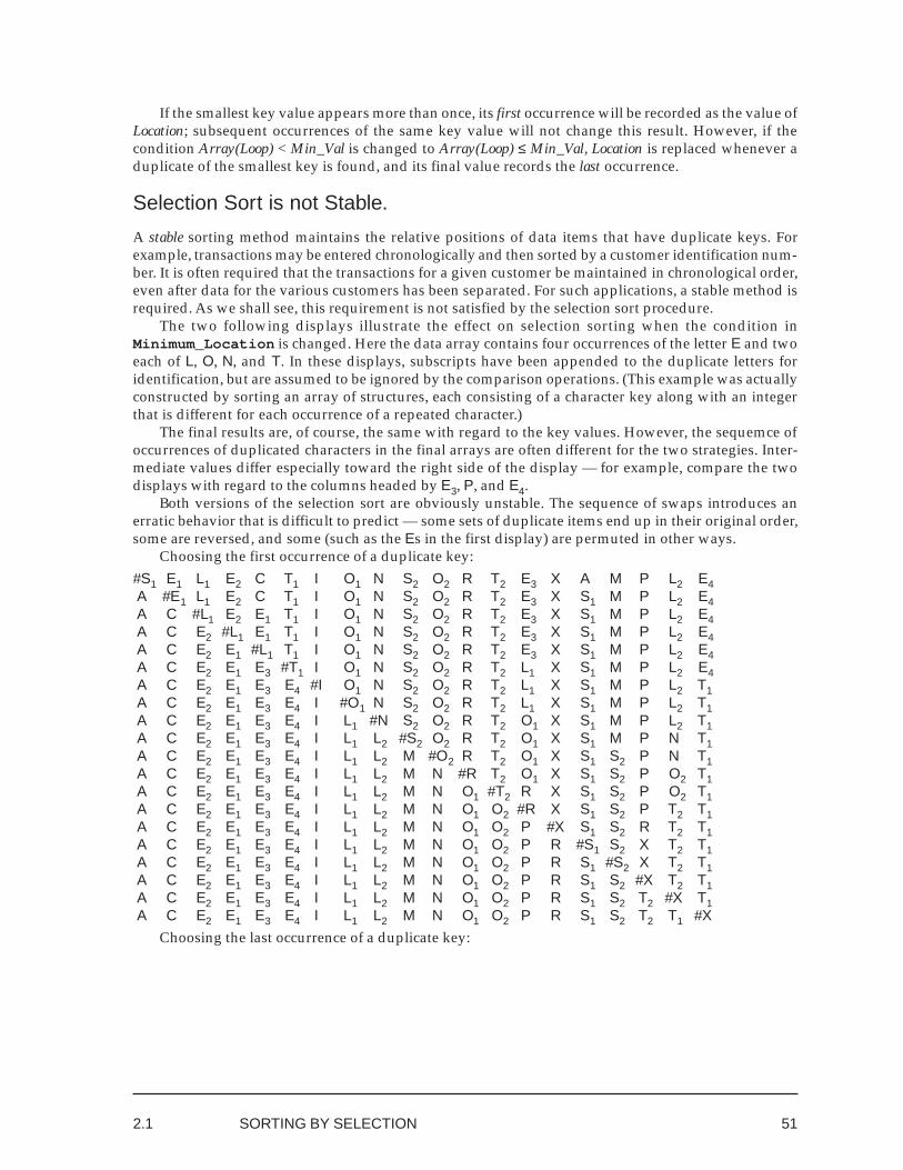
51
If the smallest key value appears more than once, its first occurrence will be recorded as the value ofLocation; subsequent occurrences of the same key value will not change this result. However, if thecondition Array(Loop) < Min_Val is changed to Array(Loop) ≤ Min_Val, Location is replaced whenever aduplicate of the smallest key is found, and its final value records the last occurrence.
Selection Sort is not Stable.
A stable sorting method maintains the relative positions of data items that have duplicate keys. Forexample, transactions may be entered chronologically and then sorted by a customer identification num-ber. It is often required that the transactions for a given customer be maintained in chronological order,even after data for the various customers has been separated. For such applications, a stable method isrequired. As we shall see, this requirement is not satisfied by the selection sort procedure.
The two following displays illustrate the effect on selection sorting when the condition inMinimum_Location is changed. Here the data array contains four occurrences of the letter E and twoeach of L, O, N, and T. In these displays, subscripts have been appended to the duplicate letters foridentification, but are assumed to be ignored by the comparison operations. (This example was actuallyconstructed by sorting an array of structures, each consisting of a character key along with an integerthat is different for each occurrence of a repeated character.)
The final results are, of course, the same with regard to the key values. However, the sequemce ofoccurrences of duplicated characters in the final arrays are often different for the two strategies. Inter-mediate values differ especially toward the right side of the display — for example, compare the twodisplays with regard to the columns headed by E3, P, and E4.
Both versions of the selection sort are obviously unstable. The sequence of swaps introduces anerratic behavior that is difficult to predict — some sets of duplicate items end up in their original order,some are reversed, and some (such as the Es in the first display) are permuted in other ways.
Choosing the first occurrence of a duplicate key:#S1 E1 L1 E2 C T1 I O1 N S2 O2 R T2 E3 X A M P L2 E4 A #E1 L1 E2 C T1 I O1 N S2 O2 R T2 E3 X S1 M P L2 E4 A C #L1 E2 E1 T1 I O1 N S2 O2 R T2 E3 X S1 M P L2 E4 A C E2 #L1 E1 T1 I O1 N S2 O2 R T2 E3 X S1 M P L2 E4 A C E2 E1 #L1 T1 I O1 N S2 O2 R T2 E3 X S1 M P L2 E4 A C E2 E1 E3 #T1 I O1 N S2 O2 R T2 L1 X S1 M P L2 E4 A C E2 E1 E3 E4 #I O1 N S2 O2 R T2 L1 X S1 M P L2 T1 A C E2 E1 E3 E4 I #O1 N S2 O2 R T2 L1 X S1 M P L2 T1 A C E2 E1 E3 E4 I L1 #N S2 O2 R T2 O1 X S1 M P L2 T1 A C E2 E1 E3 E4 I L1 L2 #S2 O2 R T2 O1 X S1 M P N T1 A C E2 E1 E3 E4 I L1 L2 M #O2 R T2 O1 X S1 S2 P N T1 A C E2 E1 E3 E4 I L1 L2 M N #R T2 O1 X S1 S2 P O2 T1 A C E2 E1 E3 E4 I L1 L2 M N O1 #T2 R X S1 S2 P O2 T1 A C E2 E1 E3 E4 I L1 L2 M N O1 O2 #R X S1 S2 P T2 T1 A C E2 E1 E3 E4 I L1 L2 M N O1 O2 P #X S1 S2 R T2 T1 A C E2 E1 E3 E4 I L1 L2 M N O1 O2 P R #S1 S2 X T2 T1 A C E2 E1 E3 E4 I L1 L2 M N O1 O2 P R S1 #S2 X T2 T1 A C E2 E1 E3 E4 I L1 L2 M N O1 O2 P R S1 S2 #X T2 T1 A C E2 E1 E3 E4 I L1 L2 M N O1 O2 P R S1 S2 T2 #X T1 A C E2 E1 E3 E4 I L1 L2 M N O1 O2 P R S1 S2 T2 T1 #X
Choosing the last occurrence of a duplicate key:
2.1 SORTING BY SELECTION
52
#S1 E1 L1 E2 C T1 I O1 N S2 O2 R T2 E3 X A M P L2 E4 A #E1 L1 E2 C T1 I O1 N S2 O2 R T2 E3 X S1 M P L2 E4 A C #L1 E2 E1 T1 I O1 N S2 O2 R T2 E3 X S1 M P L2 E4 A C E4 #E2 E1 T1 I O1 N S2 O2 R T2 E3 X S1 M P L2 L1 A C E4 E3 #E1 T1 I O1 N S2 O2 R T2 E2 X S1 M P L2 L1 A C E4 E3 E2 #T1 I O1 N S2 O2 R T2 E1 X S1 M P L2 L1 A C E4 E3 E2 E1 #I O1 N S2 O2 R T2 T1 X S1 M P L2 L1 A C E4 E3 E2 E1 I #O1 N S2 O2 R T2 T1 X S1 M P L2 L1 A C E4 E3 E2 E1 I L1 #N S2 O2 R T2 T1 X S1 M P L2 O1 A C E4 E3 E2 E1 I L1 L2 #S2 O2 R T2 T1 X S1 M P N O1 A C E4 E3 E2 E1 I L1 L2 M #O2 R T2 T1 X S1 S2 P N O1 A C E4 E3 E2 E1 I L1 L2 M N #R T2 T1 X S1 S2 P O2 O1 A C E4 E3 E2 E1 I L1 L2 M N O1 #T2 T1 X S1 S2 P O2 R A C E4 E3 E2 E1 I L1 L2 M N O1 O2 #T1 X S1 S2 P T2 R A C E4 E3 E2 E1 I L1 L2 M N O1 O2 P #X S1 S2 T1 T2 R A C E4 E3 E2 E1 I L1 L2 M N O1 O2 P R #S1 S2 T1 T2 X A C E4 E3 E2 E1 I L1 L2 M N O1 O2 P R S2 #S1 T1 T2 X A C E4 E3 E2 E1 I L1 L2 M N O1 O2 P R S2 S1 #T1 T2 X A C E4 E3 E2 E1 I L1 L2 M N O1 O2 P R S2 S1 T2 #T1 X A C E4 E3 E2 E1 I L1 L2 M N O1 O2 P R S2 S1 T2 T1 #X
Section 2.1 Exercises1. Modify Example 1 to sort an array of 12 real numbers.
2. Modify Example 2 to sort the same array by latitude instead of by city name.
2.2 SORTING BY INSERTIONIt is said that every flock of chickens has a pecking order — a social hierarchy in which each bird knows itsrank. A bird pecks another lower in the scale without fear of retaliation and submits to pecking by one ofhigher rank. When a new bird is added to the flock, a certain amount of random pecking occurs at first,but then the new bird establishes its rank and settles into the hierarchy accordingly.
The idea of sorting by insertion is to introduce new chickens (unsorted data items) into the flock oneat a time, systematically placing each new bird in its correct position before bringing in the next. Initially,the flock consists of just one chicken and the pecking order is correct by definition. The second chickenis then compared with the first chicken, which either remains at the bottom of the pecking order or risesabove the new bird. Each new bird is compared with those already in the flock to establish its rank.
Insertion sorting may be illustrated as follows:
Introduction to Sorting
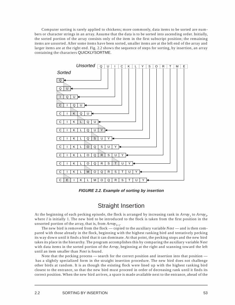
53
S O R T EQ U I C K ML Y
UQ
I UQ
C I UQ
C I K UQ
I K L QC U
K L Q YI UC
L Q S YC K UI
O Q S YC I L UK
Q R S YC I K O UL
Q R S T YC I K L O U
Q
YQ R S TC I K L O UM
Q
Unsorted
Sorted
U
I
C
K
L
Y
S
O
R
T
M
E
Computer sorting is rarely applied to chickens; more commonly, data items to be sorted are num-bers or character strings in an array. Assume that the data is to be sorted into ascending order. Initially,the sorted portion of the array consists only of the item in the first subscript position; the remainingitems are unsorted. After some items have been sorted, smaller items are at the left end of the array andlarger items are at the right end. Fig. 2.2 shows the sequence of steps for sorting, by insertion, an arraycontaining the characters QUICKLYSORTME.
FIGURE 2.2. Example of sorting by insertion
Straight InsertionAt the beginning of each pecking episode, the flock is arranged by increasing rank in Array1 to ArrayI,where I is initially 1. The new bird to be introduced to the flock is taken from the first position in theunsorted portion of the array, that is, from ArrayI+1.
The new bird is removed from the flock — copied to the auxiliary variable Next — and is then com-pared with those already in the flock, beginning with the highest ranking bird and tentatively peckingits way down until it finds a bird that it can dominate. At that point, the pecking stops and the new birdtakes its place in the hierarchy. The program accomplishes this by comparing the auxiliary variable Nextwith data items in the sorted portion of the Array, beginning at the right and scanning toward the leftuntil an item smaller than Next is found.
Note that the pecking process — search for the correct position and insertion into that position —has a slightly specialized form in the straight insertion procedure. The new bird does not challengeother birds at random. It is as though the existing flock were lined up with the highest ranking birdclosest to the entrance, so that the new bird must proceed in order of decreasing rank until it finds itscorrect position. When the new bird arrives, a space is made available next to the entrance, ahead of the
2.2 SORTING BY INSERTION
54
currently highest ranking bird. The new bird challenges the current leader; if the challenge is unsuccess-ful, the leader moves up into the new space next to the entrance and remains as the highest ranking bird.This vacates the space formerly occupied by the leader. The new bird then challenges the other birds inturn, moving along in order of decreasing rank. Whenever a challenge is unsuccessful, the challengedbird moves up, vacating its former space. When the challenge is successful, the new bird slips into thevacant space just above the bird that lost the challenge.
Each complete pecking episode increases the size of the sorted portion of the array from J to J + 1.Space at position ArrayJ+1 is made available when the first unsorted item is copied to Next. During thescan, Next is compared with ArrayI, where I begins at J and decreases. Note that ArrayI+1 is “vacant” —its value is no longer needed — at the time Next is compared with ArrayI. If Next is less than ArrayI, thatarray element is moved right by one position, into the vacant space; otherwise ArrayI remains in placeand Next is inserted at ArrayI+1, completing the scan. It may happen that all of the previously sorteditems are larger than Next, so that they are all moved and Next is inserted at Array1. Or it may happenthat Next is the new dominant item, in which case the scan terminates immediately and Next is simplystored back in ArrayJ+1.
The pecking operation is repeated for values of J from 1 to size( Array ) – 1.do J = 1, size( Array ) - 1
The first J items are sorted. Copy the first unsorted item, Array(J +1) , to Next ; call Peck to move this newitem to its correct position.
Next = Array(J + 1)call Peck( 1, J, Next )
end do:
subroutine Peck( L, R, Next)
Working from right to left in the sorted portion, Array(L: R) , the subroutine Peck moves larger items to the rightand inserts Next as a new sorted item.
do I = R, L, -1
Exit (to the end of the loop) if Next is smaller than an item in the sorted portion.
if (Array(I) <= Next) exitArray(I + 1) = Array(I)
end do
The loop terminates normally if all items in the sorted portion are larger than Next .
Array(I + 1) = Nextreturn
Operation Counts for Straight Insertion
do J = 1, size( Array ) - 1 ! 1Next = Array(J + 1) ! < 2call Peck( 1, J, Next ) ! < 3
end do ! < 4
Introduction to Sorting
55
subroutine Peck( L, R, Next )do I = R, L, -1 ! < 5
if (Array(I) <= Next) exit ! << 6Array(I + 1) = Array(I) ! << 7
end do ! << 8Array(I + 1) = Next ! < 9return ! < 10
Each iteration of the loop in the subroutine (lines 6 to 8) requires one comparison. If the exit does notoccur, the move operation at line 7 is executed.
In the “worst case,” when the given data is presented in reverse order, the early exit never occurs solines 5 to 8 perform J comparisons and J moves. There are two additional move operations, at lines 2 and9. These J comparisons and J + 2 moves are repeated for J = 1 to N – 1, where N is the size of Array. Thusthe total in the worst case is 0.5·N (N – 1) = 0.5·N2 – 0.5·N comparisons and 0.5·N (N – 1) +2·(N – 1) =0.5·N2 +1.5·N – 2 moves.
For the “average case” (random data), the loop at lines 6 to 8 will be iterated J / 2 times before exitoccurs, so lines 3 to 8 perform 0.5·J comparisons and 0.5·J – 1 moves; adding the moves at lines 2 and 9gives 0.5·J + 1 moves for the body of the outer loop, lines 2 to 4. Repeating these for J = 1 to N – 1, theaverage case total is 0.25·N2 – 0.25·N comparisons and 0.25·N2 +0.5·N – 1 moves.
Note that insertion sorting requires about half the number of comparisons and moves required byselection. This is because insertion searches a sorted array section, and thus requires only an expected0.5·J comparisons, terminating when the insertion point is found. Selection, on the other hand, searchesan unsorted array section and must examine every item.
In the “best case,” when the given data is already in the correct order, exit occurs at the first iterationof the inner loop so the total count for lines 3 to 8 is one comparison and no moves (independent of J );lines 2 to 4 require one comparison and two moves. The entire procedure requires N – 1 comparisonsand 2·N – 2 moves in the best case.
Initially Ordered Data
Straight insertion is an excellent method for large amounts of data that is already almost in order. In theextreme case of data already completely in order, each item is compared with only one other and nomove operations are required. Otherwise, the number of comparisons and moves for an item dependsonly upon the distance between its original and final positions. Benchmark time for 1 million real num-bers already in order, on a 50 MHz 486DX computer, was found to be 4 seconds.
Straight Insertion Is Stable
For straight insertion sorting, each unsorted item is compared only with items that preceded it in theoriginal unsorted array. The comparison relation causes termination of the insertion loop when a smalleror equal item is encountered. When an equal item is found, that item remains in place and the new itemis inserted on its right. (To continue searching for a strictly smaller item would exactly reverse all dupli-cate items, besides being inefficient.) Thus it can be seen that the insertion sort method, if implementedwith a bit of care, is stable.
2.2 SORTING BY INSERTION
56
I1 #N1 S1 E1 R1 T1 I2 O N2 S2 O R2 T2 E2 X A M P L E3 I1 N1 #S1 E1 R1 T1 I2 O N2 S2 O R2 T2 E2 X A M P L E3 I1 N1 S1 #E1 R1 T1 I2 O N2 S2 O R2 T2 E2 X A M P L E3 E1 I1 N1 S1 #R1 T1 I2 O N2 S2 O R2 T2 E2 X A M P L E3 E1 I1 N1 R1 S1 #T1 I2 O N2 S2 O R2 T2 E2 X A M P L E3 E1 I1 N1 R1 S1 T1 #I2 O N2 S2 O R2 T2 E2 X A M P L E3 E1 I1 I2 N1 R1 S1 T1 #O N2 S2 O R2 T2 E2 X A M P L E3 E1 I1 I2 N1 O R1 S1 T1 #N2 S2 O R2 T2 E2 X A M P L E3 E1 I1 I2 N1 N2 O R1 S1 T1 #S2 O R2 T2 E2 X A M P L E3 E1 I1 I2 N1 N2 O R1 S1 S2 T1 #O R2 T2 E2 X A M P L E3 E1 I1 I2 N1 N2 O O R1 S1 S2 T1 #R2 T2 E2 X A M P L E3 E1 I1 I2 N1 N2 O O R1 R2 S1 S2 T1 #T2 E2 X A M P L E3 E1 I1 I2 N1 N2 O O R1 R2 S1 S2 T1 T2 #E2 X A M P L E3 E1 E2 I1 I2 N1 N2 O O R1 R2 S1 S2 T1 T2 #X A M P L E3 E1 E2 I1 I2 N1 N2 O O R1 R2 S1 S2 T1 T2 X #A M P L E3 A E1 E2 I1 I2 N1 N2 O O R1 R2 S1 S2 T1 T2 X #M P L E3 A E1 E2 I1 I2 M N1 N2 O O R1 R2 S1 S2 T1 T2 X #P L E3 A E1 E2 I1 I2 M N1 N2 O O P R1 R2 S1 S2 T1 T2 X #L E3 A E1 E2 I1 I2 L M N1 N2 O O P R1 R2 S1 S2 T1 T2 X #E3 A E1 E2 E3 I1 I2 L M N1 N2 O O P R1 R2 S1 S2 T1 T2 X
Say It with Fortran
For small amounts of data, or for data that is already nearly in order, insertion sorting is very suitable forFortran (why?)
Example 5. Here, subroutine Peck has been moved in-line for efficiency. The subroutine Print_Arrayand the main program to test the module are the same as for Example 1 (except for the use statement inthe main program).
! Example 5. Sorting an array of strings by straight insertion.subroutine In_Sort( Array )
character (len = *), intent(in out), dimension(:) :: Array
The dummy argument Array has assumed shape (with rank 1), character type, and assumed length. (The arraysize and the length of the strings in the array will be taken from the actual argument.) Its intent attribute is inout , which means that the corresponding actual argument array must be definable (for example, it must not be anarray-valued expression that contains operators), and all of its elements must have defined values at entry to thesubroutine.
character (len = len( Array )) :: Nextinteger :: I, J
! start subroutine In_Sortdo J = 1, size( Array ) - 1
Next = Array(J + 1)do I = J, 1, - 1
The value of J will be retained if an exit occurs.
if (Array(I) <= Next) exitArray(I + 1) = Array(I)
end do
Introduction to Sorting
57
If the loop terminates normally, the value of I is 0 and Next is inserted at position 1.
Array(I + 1) = Nextend doreturn
end subroutine In_Sort
Insertion Sort with PointersSuppose that the structures in an array are very large. Would it be possible to sort them without movingthem? This example shows how to move a corresponding array of pointers until the first pointer points tothe item with the smallest key, etc. For purposes of illustration, in this example each data item consists ofa string (City_Name), two scalar integers (Latitude and Longitude), and an array of 1,000 integers (Stuff).(In the following example, all elements of Stuff are zero. In practice, the data to be sorted would begenerated by means that are not of concern here.)
In database terminology, the sorted array of pointers is an index to the data array. Pointer techniquescan be applied with any of the sorting methods, but it is particulary advantageous for insertion since (aswe have seen) much of the effort of this method occurs in moving the data elements.
The steps in this Sort subroutine parallel those of Example 5. The only changes are to move thepointers instead of the array elements.
Say It with Fortran
Example 6. Fortran does not provide arrays of pointers. (A variable with pointer and dimensionattributes is a pointer to an array, not an array of pointers.) However, it is possible to define a structurehaving a single component that is a pointer, and then to create an array of these structures. (See the datatype BOX in the following example.) Further examples of this technique are shown in Chapter 5.
! Example 6. Sort an array of structures by straight insertion with pointers.program D06
implicit noneinteger, parameter :: NAME_LEN = 20type :: City_Data_Type
character (len = NAME_LEN) :: City_Nameinteger :: Latitude, Longitudeinteger, dimension(1000) :: Stuff = 0
end type City_Data_Typetype :: BOX
type (City_Data_Type), pointer :: DPend type BOXinteger :: Array_Size, Looptype (City_Data_Type) Arraytype (City_Data_Type), dimension(:), allocatable, target :: Array
X(I) % DP is a pointer to City_Data_Type .
type (BOX), dimension(:), allocatable :: X
! start program D06open (1, file = "jacumba.dat", status = "old", action = "read", &
position = "rewind" )read (1, *) Array_Sizeallocate( Array(Array_Size), X(Array_Size) )
2.2 SORTING BY INSERTION
58
Load sample data into Array .
do Loop = 1, Array_Sizeread (unit = 1, fmt = "(a, 2i)" ) Array(Loop) % City_Name, &
Array(Loop) % Latitude, Array(Loop) % Longitudeend docall In_Sort( )call Print_Array( )deallocate( Array, X)stop
contains
Array, which contains the data to be sorted, is an intent(in) argument; it will not be changed during execution ofSort. The intent(out) argument X is an array of type BOX; its pointer components will be set so that the first pointerpoints to the item with the smallest key, etc..
subroutine In_Sort( )type (City_Data_Type), Pointer :: Nextinteger :: I, J
! start subroutine In_Sort
Array(1) becomes the target of the first pointer.
X(1) % DP => Array(1)do J = 1, size( Array ) - 1
The first I items are sorted. The next unsorted item becomes the target of Next .
Next => Array(J + 1)do I = J, 1, - 1
Compare the target of Next with the target of an already sorted pointer.
if (X(I) % DP % City_Name <= Next % City_Name) exit
Move a pointer. (Note that elements of Array never move.)
X(I + 1) % DP => X(I) % DPend do
Copy Next to insert it among the sorted pointers.
X(I + 1) % DP => Nextend doreturn
end subroutine In_Sort
subroutine Print_Array( X )integer :: I
! start subroutine Print_Arraydo I = 1, size( X )
Print components of the target of X(I) % DP, including an arbitrary component of the array Stuff
print *, I, ': "', X(I) % DP % City_Name, '" ', &X(I) % DP % Latitude, X(I) % DP % Longitude, X(I) % DP % Stuff(17)
end doreturn
end subroutine Print_Array
end program D06
Introduction to Sorting
59
Insertion during InputSome applications read data from an external file and sort it. The two operations can be combined, asshown in this example. For sorting during input, the insertion method is especially well suited, becauseit considers the unsorted items one at a time. Furthermore, for some applications the total time requiredmay be dominated by the input phase so that the comparison and move operations cost nothing.
Expanding array.
The structure Elastic in this program illustrates use of an expanding array to hold a variable amount ofdata. The maximum amount of data that can be processed is limited by the size of the array, which isfixed at the time the array is created. It is convenient to enclose an expanding array in a structure alongwith an integer that holds the current length — i.e., the current number of array elements to whichactual data has been assigned. The (maximum) array size is also recorded in the structure.
Say It with Fortran
Example 7.
! Example 7. Sort structures by straight insertion during input.program D07
implicit noneinteger, parameter :: NAME_LEN = 20type :: City_Data_Type
character (len = NAME_LEN) :: City_Nameinteger :: Latitude, Longitudeinteger, dimension(1000) :: Stuff = 0
end type City_Data_Type
The derived type Elastic holds the expanding array of structures along with an integer, Current_Length ,that records the current number of array elements to which actual data has been assigned. The (maximum) arraysize is also recorded in the structure for convenience.13
type :: Elastictype (City_Data_Type), dimension (:), pointer :: Array
Initialize Current_Length to zero .
integer :: Current_Length = 0, Maximum_Lengthend type Elastictype (Elastic) :: A
! start program D07open (1, file = "jacumba.dat", status = "old", action = "read" &
position = "rewind" )read (1, *) A % Maximum_Lengthallocate( A % Array(A % Maximum_Length) )call Read_And_Sort( )
13 It should be noted that a standard Technical Report on Enhanced Derived Type Facilities supports allocatablearrays as derived type components; with Fortran versions that do not implement this report, pointers may beemployed instead.
Component initialization in a derived type definition is a Fortran 95 enhancement; for versions that do notimplement this feature, the declared initialization must be replaced by assignment statements in the mainprogram.
2.2 SORTING BY INSERTION
60
call Print_Array( )deallocate( A % Array )stop
contains
subroutine Read_And_Sort( )type (City_Data_Type) :: Nextinteger :: I, J, EoF
! start subroutine Read_And_Sortdo J = 0, A % Maximum_Length - 1
read (1, "(a, i3, i4)", iostat = EoF) Next % City_Name, &Next % Latitude, Next % Longitude
if (EoF < 0) exitdo I = J, 1, - 1
Compare and move operations involve the array Array , which is a component of the structure A of type Elas-tic .
if (A % Array(I) % City_Name <= Next) exitA % Array(I + 1) = A % Array(I)
end doA % Array(I + 1) = NextA % Current_Length = J + 1
end doreturn
end subroutine Read_And_Sort
subroutine Print_Array( )integer :: I
! start subroutine Print_Arraydo I = 1, A % Current_Length
print *, I, ": ", A % Array(I) % City_Name, &A % Array(I) % Latitude, A % Array(I) % Longitude, &A % Array(I) % Stuff(17)
end doreturn
end subroutine Print_Array
end program D07
Binary InsertionAny of the insertion methods that have been described, when applied to random data, compare the Jthnew item with about J/2 sorted items. The expected number of comparisons can be reduced to lg J withbinary searching. (Knuth notes that the idea of binary insertion was described by Mauchly as early as1946 in a paper on nonnumerical computing.)
The steps must be reorganized a bit to separate the search process from the move operation. Insteadmoving up the sorted items one by one as they are found to exceed the new item, they are all moved uptogether after the insertion point has been located.
The binary search function (displayed earlier) is applied to the array of items that are already sorted,to obtain a 2-element vector. The second element of the result vector locates the smallest previouslysorted item (or possibly a rather arbitrary one of two or more equal smallest items) that is at least as largeas the new unsorted item to be inserted.
Introduction to Sorting
61
do J = 1, size( Array ) - 1
Array(1: J) contains previously sorted data.
Next = Array(J + 1)
Use binary search to locate Next in the array section Array(1: J) . The insertion point, returned as Location(2),is between 1 and J +1, inclusive.
Location = Binary_Search( Array(: J), Next )
Move all items between Array(Location(2)) and Array(J) one position to the right; insert Next atArray(Location) . Note that nothing is moved if Location(2) is J +1.
Array(Location(2) + 1: J + 1) = Array(Location(2) : J)Array(Location(2)) = Next
end do
Example 8.The program examples distributed electronically include an expanded implementation of binary
insertion during input. This algorithm will later be compared with linked list and tree algorithms for thesame application.
Binary Insertion Is Not Stable
A disadvantage for some applications is that this method is not stable for duplicate items.
Operation Counts for Binary Insertion
do J = 1, size( Array ) - 1 ! 1Next = Array(J + 1) ! < 2Location = Binary_Search( 1, J, Next ) ! < 3Array(Location(2) + 1: J + 1) = Array(Location(2) : J) ! < 4Array(Location(2)) = Next ! < 5
end do ! < 6In the average case, with arguments ( 1, J, Next ) , 1.5·(lg( J +1 ) –1) compares and no moves are
required; the array section assignment performs 0.5·I moves. The loop body (lines 2 – 6) performs 1.5·(lg(J +1 ) – 1) compares and 0.5·I +2 moves. This must be summed for J from 1 to N – 1, where N is the arraysize.
Let k = J + 1; the loop is executed with k = 2 to N, so the sum isN lg N – 2·lg 2 – 1.4·(N – 2) = N lg N – 1.4·N + 0.8
Comparisons: 1.5·N lg N – 2.1·N – 0.3Moves: 0.25 N (N – 1) +2.0 (N – 1) = 0.25 N2 +1.75·N – 2The search scheme employed here is efficient — about 1.5 N lg N total comparisons — but it re-
quires slightly more move operations, 0.25·N2 +1.75·N – 2, than straight insertion. However, modernpipeline and parallel processors can move contiguous array sections at high speed.
In the worst case, when the data is in reverse order, the array section assignment makes twice asmany moves as straight insertion, in total 0.5·N2 +1.5·N – 2. In the best case, when the data is already inorder, the array section assignment moves nothing so the total move count is 2.0 N – 2.0. For sorting alarge amount of data that is almost in order, the 1.5 N lg N comparison count makes binary insertioninferior to straight insertion.
A benchmark, run with a 50 MHz 486DX computer, sorted 20,000 random real numbers in 65 sec-onds.
2.2 SORTING BY INSERTION
62
2.3 SHELL SORTDonald Shell in 1959 proposed a “diminishing increment” sort method. As Sedgwick explains, “Inser-tion sort is slow because it exchanges only adjacent elements. For example, if the smallest element hap-pens to be at the end of the array, N steps are needed to get it where it belongs. Shell sort is a simpleextension of insertion sort which gains speed by allowing exchanges of elements that are far apart.”14
Shell sort consists of a sequence of insertion sorts applied to nonconsecutive sections of the givenarray. At first, widely spaced elements are sorted by insertion. The spacing is then diminished until thefinal stage, which is a straight insertion sort of the entire array. The effect of the earlier stages is toguarantee that the array is almost in order before the final sort is applied.
Various increment sequences are possible. A popular sequence employs integers of the form floor(3p/2 ), beginning with the largest such value that does not exceed the array size. For example, if thearray size is more than 29,524 but less than 88,573 the sequence is 29,524, 9,841, 3,280, 1,093, 364, 121, 40,13, 4, 1. Note that 3p is odd for any positive integer p, so floor( 3p/2 ) = (3p – 1) / 2. The initial incrementcan be calculated as pmax = log3( 2·N + 1 ) = log3( e )·ln( 2·N + 1):
P_Max = int( LOG3_OF_E * log( 2.0 * N + 1.0 ) )do P = P_Max, 1, -1
H = (3 ** P) / 2do J = 1, N - H
Next = Array(J + H)do I = J, 1, -H
if (Array(I) <= Next) exitArray(I + H) = Array(I)
end doArray(I + H) = Next
end doend do
Suppose that 13 ≤ N < 40 (for example, N = 28) so that the increment sequence is 13, 4, 1; andconsider the second stage, when the increment is 4. This stage begins by comparing position 5 withposition 1; later on, position 9 is compared with the sorted sequence in positions (5, 1); position 13 iscompared with the “chain” of sorted data at positions (9, 5, 1); position 17 is compared with the chain(13, 9, 5, 1); position 21 is compared with the chain (17, 13, 9, 5, 1); and finally position 25 is comparedwith the chain (21, 17, 13, 9, 5, 1). The effect is a straight insertion sort of the chain (25, 21, 17, 13, 9, 5, 1).
The straight insertion sorts (for a given increment) are are interleaved. For example, elements inpositions between 21 and 25 are examined as they naturally occur. Immediately after element 21 isinserted into the chain (17, 13, 9, 5, 1), the next step is to insert element 22 into the chain (18, 14, 10, 6, 2),then to insert element 23 into the chain (19, 15, 11, 7, 3), and so on.
Shell sort is not a stable sorting method.
Operation Counts for Shell Sort
The running time for Shell sort is very difficult to predict, and is known to depend heavily upon theincrement sequence. Sedgewick states that N1.5 is a provable upper bound on the number of compari-sons for a wide variety of sequences including the one given here; for other carefully chosen incrementsequences the bound N4/3 can be proved and N7/6 is conjectured empirically.
A benchmark, run with a 50 MHz 486DX computer, sorted 1 million random real numbers in 201seconds. This timing is consistent with an estimate of 1.2·N1.3 comparison operations and the same num-ber of move operations.
14 R. Sedgewick, Algorithms, Second Ed. [Reading: Addison-Wesley, 1988], 107.
Introduction to Sorting
63
Shell Sort with Array SectionsExample 9. It is possible to subdivide the outer do construct so that each chain is separately com-pletely ordered:
do K = 1, min( H, N - H )do J = K, N - H, H
Next = Array(J + H)do I = J, 1, -H
if (Array(I) <= Next) exitArray(I + H) = Array(I)
end doArray(I + H) = Next
end doend do
The two inner loops can now be replaced by a call to In_Sort with a noncontiguous array sectionargument. In_Sort is the normal straight insertion sort procedure (as in Example 5) with an assumedshape array dummy argument. From the viewpoint of In_Sort , the dummy argument is a contiguousarray object; the loop increment value inside the procedure In_Sort is one.
Say It with Fortran
When the increment value is H, the following modified Shell sort procedure makes H calls to In_Sortwith different array sections that all have stride H:
! Example 9. Shell Sort with array Sectionssubroutine Sh_Sort( Array )
real, intent(in out), dimension(:) :: Arrayinteger :: N, P_Max, P, H, Kreal, parameter :: LOG3_OF_E = 0.9102392227
! start subroutine Sh_SortN = size( Array )P_Max = LOG3_OF_E * log( 2.0 * N + 1.0 )do P = P_Max, 1, -1
H = (3 ** P) / 2do K = 1, min( H, N - H )
Call straight insertion sort procedure. The actual argument is an array section whose stride is the current Shell sortincrement. See the discussion of Explicit Interface, below.
call In_Sort( Array(K: N : H) ) ! Array sectionend do
end doreturn
end subroutine Sh_Sort
Explicit Interface
Under certain conditions, reference to a procedure requires that interface information for the procedurebe explicit at the point of reference (see any complete Fortran 90 or 95 handbook or textbook; for ex-ample, Appendix D.6 in Fortran 90 by Meissner). One such condition is the appearance of a dummyargument that is an assumed shape array, like In_Sort in this example. Other conditions that requireexplicit interface information are pointer arguments, optional or keyword arguments, and function re-sults whose properties are established during execution.
2.3 SHELL SORT
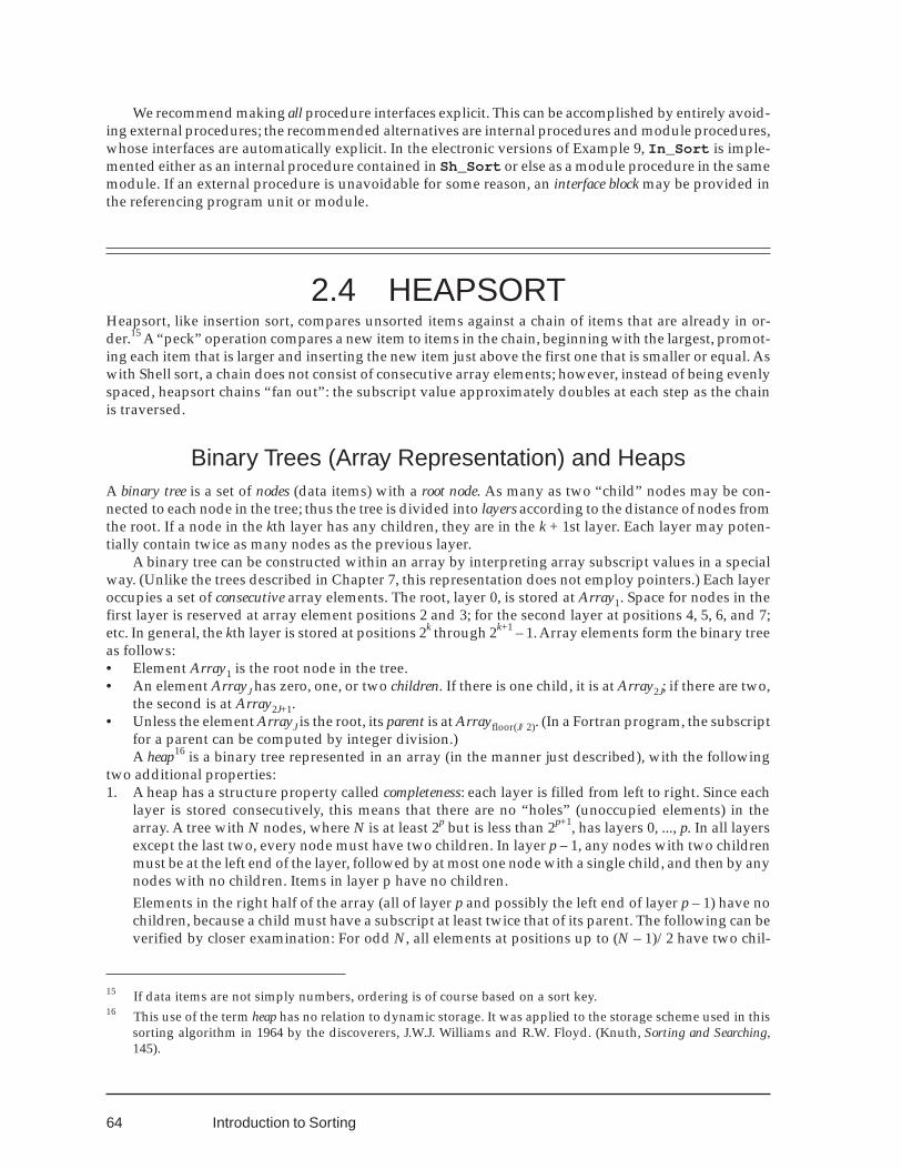
64
We recommend making all procedure interfaces explicit. This can be accomplished by entirely avoid-ing external procedures; the recommended alternatives are internal procedures and module procedures,whose interfaces are automatically explicit. In the electronic versions of Example 9, In_Sort is imple-mented either as an internal procedure contained in Sh_Sort or else as a module procedure in the samemodule. If an external procedure is unavoidable for some reason, an interface block may be provided inthe referencing program unit or module.
2.4 HEAPSORTHeapsort, like insertion sort, compares unsorted items against a chain of items that are already in or-der.15 A “peck” operation compares a new item to items in the chain, beginning with the largest, promot-ing each item that is larger and inserting the new item just above the first one that is smaller or equal. Aswith Shell sort, a chain does not consist of consecutive array elements; however, instead of being evenlyspaced, heapsort chains “fan out”: the subscript value approximately doubles at each step as the chainis traversed.
Binary Trees (Array Representation) and HeapsA binary tree is a set of nodes (data items) with a root node. As many as two “child” nodes may be con-nected to each node in the tree; thus the tree is divided into layers according to the distance of nodes fromthe root. If a node in the kth layer has any children, they are in the k + 1st layer. Each layer may poten-tially contain twice as many nodes as the previous layer.
A binary tree can be constructed within an array by interpreting array subscript values in a specialway. (Unlike the trees described in Chapter 7, this representation does not employ pointers.) Each layeroccupies a set of consecutive array elements. The root, layer 0, is stored at Array1. Space for nodes in thefirst layer is reserved at array element positions 2 and 3; for the second layer at positions 4, 5, 6, and 7;etc. In general, the kth layer is stored at positions 2k through 2k+1 – 1. Array elements form the binary treeas follows:• Element Array1 is the root node in the tree.• An element ArrayJ has zero, one, or two children. If there is one child, it is at Array2J; if there are two,
the second is at Array2J+1.• Unless the element ArrayJ is the root, its parent is at Arrayfloor(J/2). (In a Fortran program, the subscript
for a parent can be computed by integer division.)A heap16 is a binary tree represented in an array (in the manner just described), with the following
two additional properties:1. A heap has a structure property called completeness: each layer is filled from left to right. Since each
layer is stored consecutively, this means that there are no “holes” (unoccupied elements) in thearray. A tree with N nodes, where N is at least 2p but is less than 2p+1, has layers 0, ..., p. In all layersexcept the last two, every node must have two children. In layer p – 1, any nodes with two childrenmust be at the left end of the layer, followed by at most one node with a single child, and then by anynodes with no children. Items in layer p have no children.Elements in the right half of the array (all of layer p and possibly the left end of layer p – 1) have nochildren, because a child must have a subscript at least twice that of its parent. The following can beverified by closer examination: For odd N, all elements at positions up to (N – 1)/2 have two chil-
15 If data items are not simply numbers, ordering is of course based on a sort key.16 This use of the term heap has no relation to dynamic storage. It was applied to the storage scheme used in this
sorting algorithm in 1964 by the discoverers, J.W.J. Williams and R.W. Floyd. (Knuth, Sorting and Searching,145).
Introduction to Sorting
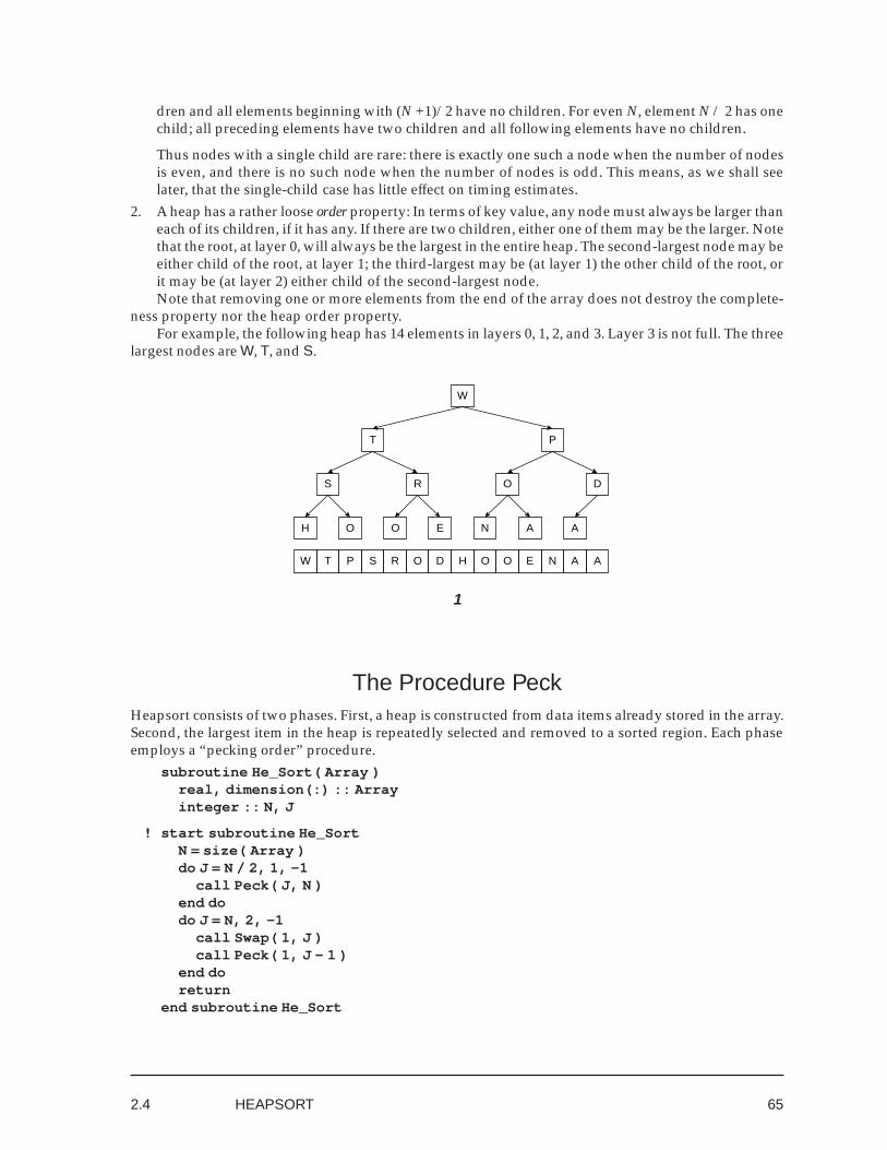
65
dren and all elements beginning with (N +1)/2 have no children. For even N, element N / 2 has onechild; all preceding elements have two children and all following elements have no children.
Thus nodes with a single child are rare: there is exactly one such a node when the number of nodesis even, and there is no such node when the number of nodes is odd. This means, as we shall seelater, that the single-child case has little effect on timing estimates.
2. A heap has a rather loose order property: In terms of key value, any node must always be larger thaneach of its children, if it has any. If there are two children, either one of them may be the larger. Notethat the root, at layer 0, will always be the largest in the entire heap. The second-largest node may beeither child of the root, at layer 1; the third-largest may be (at layer 1) the other child of the root, orit may be (at layer 2) either child of the second-largest node.Note that removing one or more elements from the end of the array does not destroy the complete-
ness property nor the heap order property.For example, the following heap has 14 elements in layers 0, 1, 2, and 3. Layer 3 is not full. The three
largest nodes are W, T, and S.
DORSPTW AANEOOH
D
O AH E A
P
S OR
T
NO
W
1
The Procedure PeckHeapsort consists of two phases. First, a heap is constructed from data items already stored in the array.Second, the largest item in the heap is repeatedly selected and removed to a sorted region. Each phaseemploys a “pecking order” procedure.
subroutine He_Sort( Array )real, dimension(:) :: Arrayinteger :: N, J
! start subroutine He_SortN = size( Array )do J = N / 2, 1, -1
call Peck( J, N )end dodo J = N, 2, -1
call Swap( 1, J )call Peck( 1, J - 1 )
end doreturn
end subroutine He_Sort
2.4 HEAPSORT
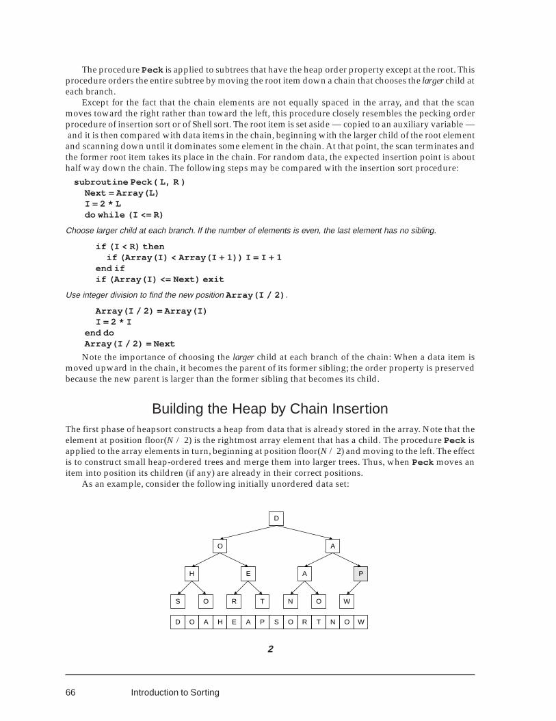
66
PAEHAOD WONTROS
D
O A
H E A P
S O R T N O W
The procedure Peck is applied to subtrees that have the heap order property except at the root. Thisprocedure orders the entire subtree by moving the root item down a chain that chooses the larger child ateach branch.
Except for the fact that the chain elements are not equally spaced in the array, and that the scanmoves toward the right rather than toward the left, this procedure closely resembles the pecking orderprocedure of insertion sort or of Shell sort. The root item is set aside — copied to an auxiliary variable —and it is then compared with data items in the chain, beginning with the larger child of the root elementand scanning down until it dominates some element in the chain. At that point, the scan terminates andthe former root item takes its place in the chain. For random data, the expected insertion point is abouthalf way down the chain. The following steps may be compared with the insertion sort procedure:
subroutine Peck( L, R )Next = Array(L)I = 2 * Ldo while (I <= R)
Choose larger child at each branch. If the number of elements is even, the last element has no sibling.
if (I < R) thenif (Array(I) < Array(I + 1)) I = I + 1
end ifif (Array(I) <= Next) exit
Use integer division to find the new position Array(I / 2) .
Array(I / 2) = Array(I)I = 2 * I
end doArray(I / 2) = Next
Note the importance of choosing the larger child at each branch of the chain: When a data item ismoved upward in the chain, it becomes the parent of its former sibling; the order property is preservedbecause the new parent is larger than the former sibling that becomes its child.
Building the Heap by Chain InsertionThe first phase of heapsort constructs a heap from data that is already stored in the array. Note that theelement at position floor(N / 2) is the rightmost array element that has a child. The procedure Peck isapplied to the array elements in turn, beginning at position floor(N / 2) and moving to the left. The effectis to construct small heap-ordered trees and merge them into larger trees. Thus, when Peck moves anitem into position its children (if any) are already in their correct positions.
As an example, consider the following initially unordered data set:
Introduction to Sorting
2
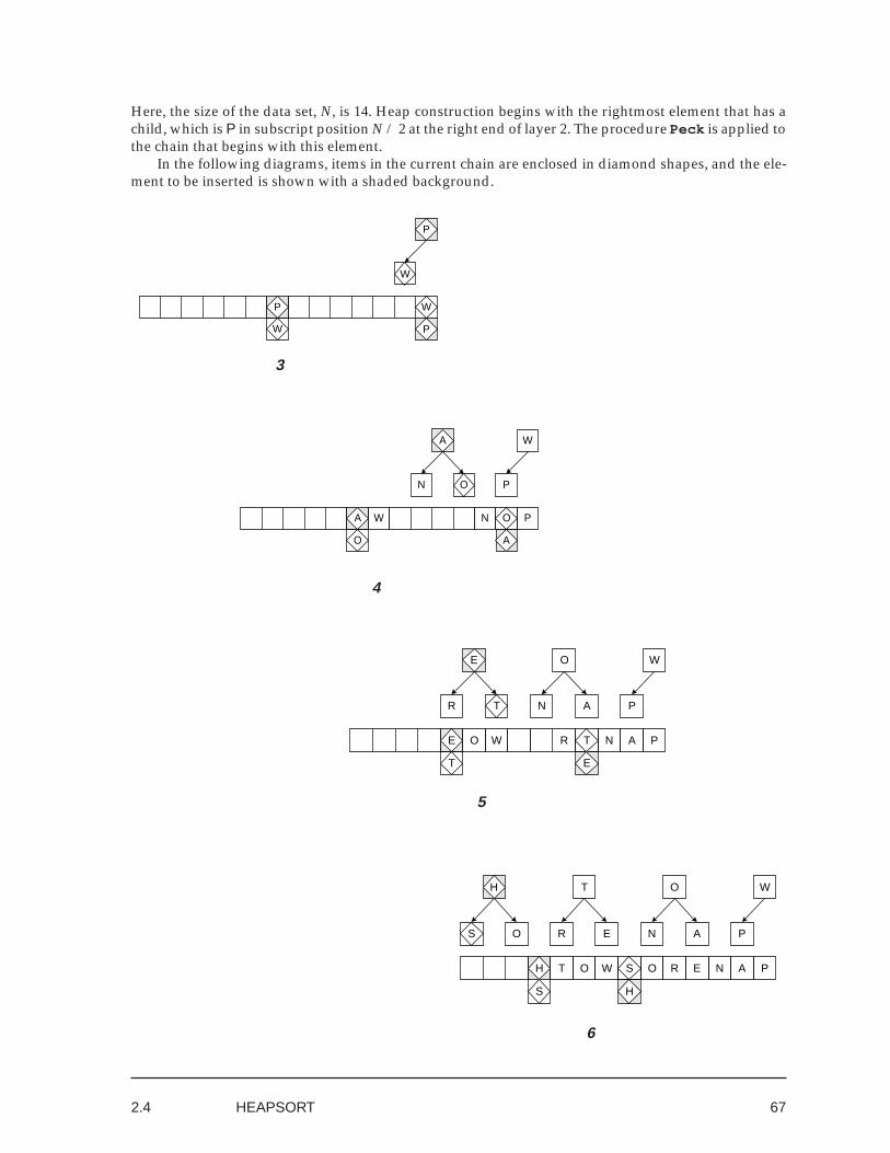
67
O WE N A PR
E
E
T
T
T
A PR N
O W
S
S
S
OT W NR AE PO
H
H
H
E A P
O
R
T
NO
W
Here, the size of the data set, N, is 14. Heap construction begins with the rightmost element that has achild, which is P in subscript position N / 2 at the right end of layer 2. The procedure Peck is applied tothe chain that begins with this element.
In the following diagrams, items in the current chain are enclosed in diamond shapes, and the ele-ment to be inserted is shown with a shaded background.
3
P
W
W
W
P
P
5
W
A
A
O
PON
A
O PN
W
6
4
2.4 HEAPSORT
68
W
W
ORST NOH AEO
W
P
P
P
A
A
A
D
D
D
O
H E A
S
O
R
T
NO
PW OR DST NOH AEO A
DO
AH E A
P
S
O
R
T
NO
W
7
8
9
10
P
P
OTS NRH AEO P
W
W
W
A
A
A
H E A
S
O R
T
N
O
T
T
T
W O PS NH AE AO
R
R
R
O
O
O
AH E A
S O P
NO
W
Introduction to Sorting
69
11
PT OR DOS
P O DO NH EA
NOH AEA
A
A
A
S
R
O
S R O
S R O
DO
H EA
P
N
O
WT
NOH AE
W P OR DST NOH AEO A
P OR DA
A
A
T
S
O
T S O
T S O
DO
H E A
P
O
R
N
W
12
2.4 HEAPSORT
It may be verified that the result is a heap with the required structure and loose order properties.
Sorting the Heap by SelectionAfter the heap has been constructed, the second phase begins. As mentioned earlier, because of the heaporder property the largest item is now the root element, Array1.
This phase resembles selection sort in that it repeatedly finds the largest item in the (unsorted) heap,removes it from the heap, and stores it as the smallest sorted item. Because of the loose order property ofthe heap, a chain of only lg J elements must be traversed to reorder the heap so that the largest of J itemsis in the root position.
A sorted section is constructed, beginning at the right end of the array. For each value of J from Ndown to 2, the largest remaining item, at Array1, is removed from the heap and is added to the sortedsection at ArrayJ. The operation actually performed is to swap ArrayJ with Array1. This removes ArrayJfrom the heap and decreases the size of the heap by one item while maintaining the heap structureproperty.
The swap operation does not reorder any of the items in the heap except the one just moved toArray1. Applying the procedure Peck to the chain beginning at Array1 restores heap order and againguarantees that the largest unsorted item is at the root.
So long as J (the number of items in the heap) is two or more, J is decreased by one and the processis repeated. In the following diagrams, the first two rows at the bottom show the heap before the swapand the entire array after the swap. As before, diamonds indicate the pecking chain, and the item en-closed in a diamond with a shaded background is the one that is to be inserted.
70
PR OO DNO
O DNO AH A
AH EA
E
E
E
OP
OP
O
P
D
O
AH A
N O
R WS T
13
OP EO DNO
O E DN H A
AH A
A
A
A
OO
OO
O
O
D
H
E
A
N
O
RP S T W
14
15
Introduction to Sorting
PS OO DOR
P OO D A EA
NAH EA
N
N
N
R
O
H
R O H
R O H
D
A EA
P
O O
T WS
71
16
OO EA DHN
A DHN
A
A
A
A
EO
EO
E
O
DH A
N
O SR TPO W
17
D
E AA
EO AA DHN
D
D
D
HN
HN
H
N
A
E
A
O RPOO WTS
18
2.4 HEAPSORT
OO EA DNO
OA EA D
H A
A
A
HNO
HNO
H
N
O
D
O
A E
O SR TP W
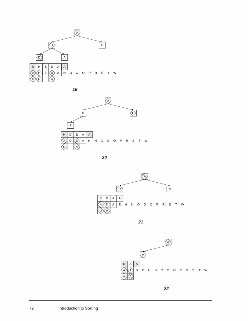
72
19
A
AE AD
A
A
A
D
D
D A
NE OH PO RO T WS
20
AD A
A
A
A
A
A
A
D E H N O O O P R S T W
21
22
AD
EH AAD
A
A
A
E
E
ED
A
N OH O PO S TR W
Introduction to Sorting
E A
EN AADH
A
A
A
H
D
H D
H D
E
A
R TPO OON WS
73
23
During this second selection phase, insertion of items into the chain is definitely not random — in thisexample, A occurs as the item to be inserted on 10 of the 13 occasions. The item to be inserted has justbeen swapped into the root position from the last layer of the tree, so it is likely to be much smaller thanaverage and insertion is unlikely to occur until almost the end of the chain.
Operation Counts for Heapsort
N = size( Array ) ! 1do J = N / 2, 1, -1 ! 2
call Peck( J, N ) ! 3end do ! 4do J = N, 2, -1 ! 5
call Swap( 1, J ) ! 6call Peck( 1, J -1 ) ! 7
end do ! 8
subroutine Peck( L, R )Next = Array(L) ! 9I = 2 * L ! 10do while (I <= R) ! 11
if (I < R) then ! 12if (Array(I) < Array(I + 1)) I = I + 1 ! 13
end if ! 14if (Array(I) <= Next) exit ! 15Array(I / 2) = Array(I) ! 16I = 2 * I ! 17
end do ! 18Array(I / 2) = Next ! 19
At line 13, the two siblings ArrayI and ArrayI+1 are compared unless ArrayI has no sibling (a case thatis rare enough to have no significant effect upon timing, as noted earlier).
The loop at lines 11 – 18 processes a chain of approximate length (lg R – lg L), but may exit beforereaching the end of the chain. Each iteration requires two data item comparisons and one move, exceptfor the last iteration in case of early exit.
As described earlier, by analogy to the integral the sum of logarithms ∑i=ab lg i can be estimated as b
lg b – a lg a – 1.4·(b – a).• First phase, building the heap by insertion, lines 1 – 4: ∑i=N/2
1 Pecki,N
For random data, exit during the first phase is expected at the midpoint of each chain. Thus theoperation count for Peck consists of one move (line 9), plus two comparisons and one move for eachiteration of lines 11 – 18. The number of iterations is
∑i=N/21 0.5·(lg N – lg i)
= 0.5·∑i=N/21 lg N – 0.5·∑i=N/2
1 lg i= 0.25·N lg N – 0.5·(0.5·N (lg N – lg 2)) – lg 1 – 1.4·(0.5·N) + 1.4)= 0.25·N +0.35·N – 0.7 (Note that the terms in N lg N cancel.)= 0.6·N – 0.7
2.4 HEAPSORT
A A
A
A
A
A D E H N O O O P R S T W
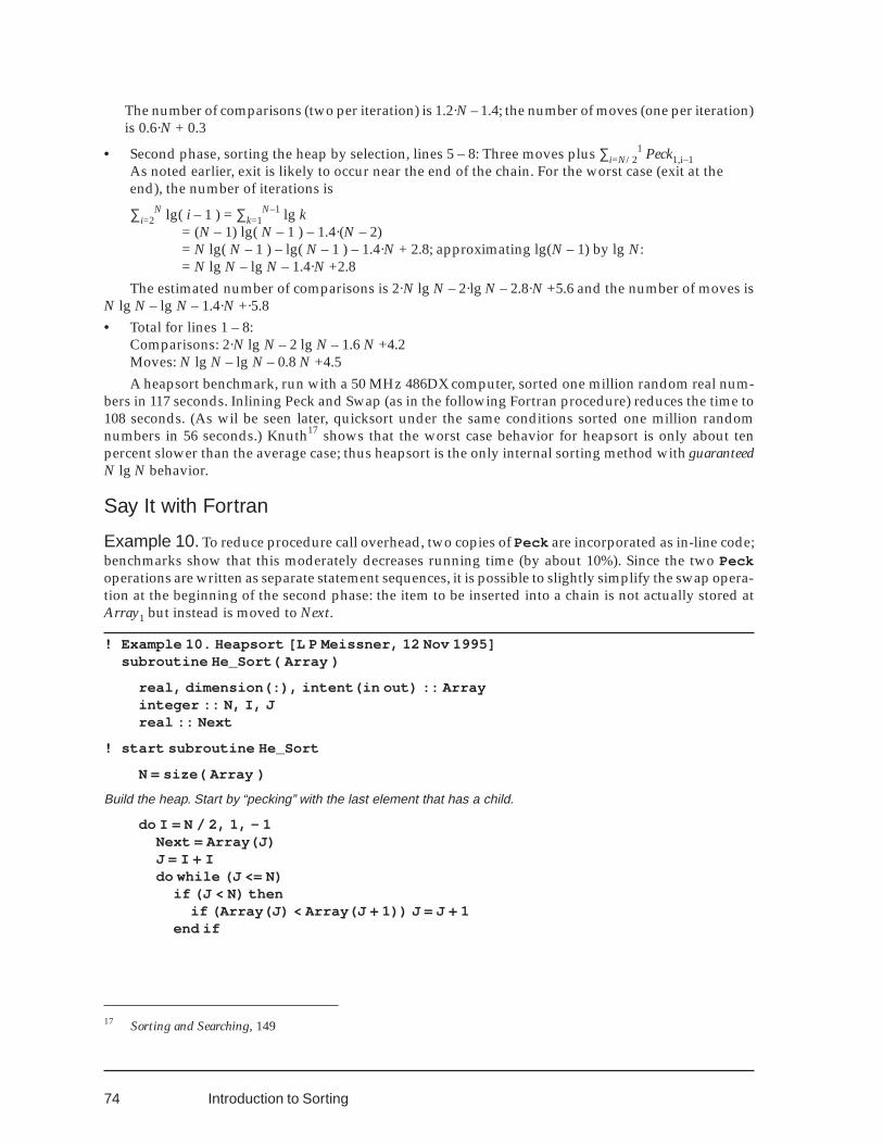
74
The number of comparisons (two per iteration) is 1.2·N – 1.4; the number of moves (one per iteration)is 0.6·N + 0.3
• Second phase, sorting the heap by selection, lines 5 – 8: Three moves plus ∑i=N/21 Peck1,i–1
As noted earlier, exit is likely to occur near the end of the chain. For the worst case (exit at theend), the number of iterations is
∑i=2N lg( i – 1 ) = ∑k=1
N–1 lg k= (N – 1) lg( N – 1 ) – 1.4·(N – 2)= N lg( N – 1 ) – lg( N – 1 ) – 1.4·N + 2.8; approximating lg(N – 1) by lg N:= N lg N – lg N – 1.4·N +2.8
The estimated number of comparisons is 2·N lg N – 2·lg N – 2.8·N +5.6 and the number of moves isN lg N – lg N – 1.4·N +·5.8• Total for lines 1 – 8:
Comparisons: 2·N lg N – 2 lg N – 1.6 N +4.2Moves: N lg N – lg N – 0.8 N +4.5A heapsort benchmark, run with a 50 MHz 486DX computer, sorted one million random real num-
bers in 117 seconds. Inlining Peck and Swap (as in the following Fortran procedure) reduces the time to108 seconds. (As wil be seen later, quicksort under the same conditions sorted one million randomnumbers in 56 seconds.) Knuth17 shows that the worst case behavior for heapsort is only about tenpercent slower than the average case; thus heapsort is the only internal sorting method with guaranteedN lg N behavior.
Say It with Fortran
Example 10. To reduce procedure call overhead, two copies of Peck are incorporated as in-line code;benchmarks show that this moderately decreases running time (by about 10%). Since the two Peckoperations are written as separate statement sequences, it is possible to slightly simplify the swap opera-tion at the beginning of the second phase: the item to be inserted into a chain is not actually stored atArray1 but instead is moved to Next.
! Example 10. Heapsort [L P Meissner, 12 Nov 1995]subroutine He_Sort( Array )
real, dimension(:), intent(in out) :: Arrayinteger :: N, I, Jreal :: Next
! start subroutine He_Sort
N = size( Array )
Build the heap. Start by “pecking” with the last element that has a child.
do I = N / 2, 1, - 1Next = Array(J)J = I + Ido while (J <= N)
if (J < N) thenif (Array(J) < Array(J + 1)) J = J + 1
end if
17 Sorting and Searching, 149
Introduction to Sorting
75
if (Array(I) <= Next) exitArray(J / 2) = Array(J)J = J + I
end doArray(J / 2) = Next
end do
Now sort by selection. Move Array(1) to the sorted portion, then restore the heap order property.
do I = N, 2, - 1Next = Array(I)Array(I) = Array(1)J = 2do while (J < I)
if (J < I - 1) thenif (Array(J) < Array(J + 1)) J = J + 1
end ifif (Array(J) <= Next) exitArray(J / 2) = Array(J)J = J + I
end doArray(J / 2) = Next
end doreturn
end subroutine He_Sort
2.5 OPERATION COUNTS FOR SORTING:SUMMARY
SwapComparisons: 0Moves: 3
Swap with test; p is the probability that the items to be exchanged are actually different.Comparisons: 1Moves: 3p
Min_LocationComparisons: N – 1Moves: = 0.7·lgN + 0.6
Binary_SearchComparisons: 1.5·lg N – 1.5Moves: 0
Sort_3Comparisons: 3Moves: 4.5
2.4 HEAPSORT
76
Sorting Methods Described So Far (Slower to Faster)
Benchmark results are consistent with about ½ million compares or 1½ million moves per second on a 50MHz 486DX. These numbers include the accompanying overhead.Se_Sort (selection)
Comparisons: 0.5·N2 +0.5·N – 1Moves: 0.7·N lg (N – 1) + 5.6·N – 0.7·lg (N – 1) – 6.6Benchmark time for 20,000 random real numbers: 350 seconds
In_Sort (straight insertion)Timing is strongly data-dependent.Average Case (random data):
Comparisons: 0.25·N2 – 0.25·NMoves: 0.25·N2 +0.5·N – 1Benchmark time for 20,000 random real numbers: 291 seconds.
Best Case (data in order)Comparisons: N – 1Moves: 2·N – 2
Benchmark time for 1 million real numbers already in order: 4 secondsWorst Case (data in reverse order)
Comparisons: 0.5·N2 – 0.5·NMoves: 0.5·N2 +1.5·N – 2
Binary Insertion with block move.Timing is strongly data-dependent.Average Case (random data):
Comparisons: 1.5·N lg N – 2.1·N – 0.3Moves: 0.25·N2 + 1.75·N – 2Benchmark time for 20,000 random real numbers: 65 seconds.
Best Case (data in order)Comparisons: 1.5·N lg N – 2.1·N – 0.3Moves: 2·N – 2
Worst Case (data in reverse order)Comparisons: 1.5·N lg N – 2.1·N – 0.3Moves: 0.5·N2 + 1.5·N – 2
Sh_Sort (Shell sort) with array sections. Conjectured operation counts are based on benchmark.Timing is dependent on choice of intervals.Comparisons: 1.2·N1.3
Moves: 1.2·N1.3
Benchmark time for 1 million random real numbers: 201 seconds
He_Sort (heapsort)Comparisons: 2·N lg N – 1.6·N – 2·lg N + 4.2Moves: N lg N – 0.8·N – lg N + 4.5Benchmark time for 1 million random real numbers: 104 seconds
Introduction to Sorting
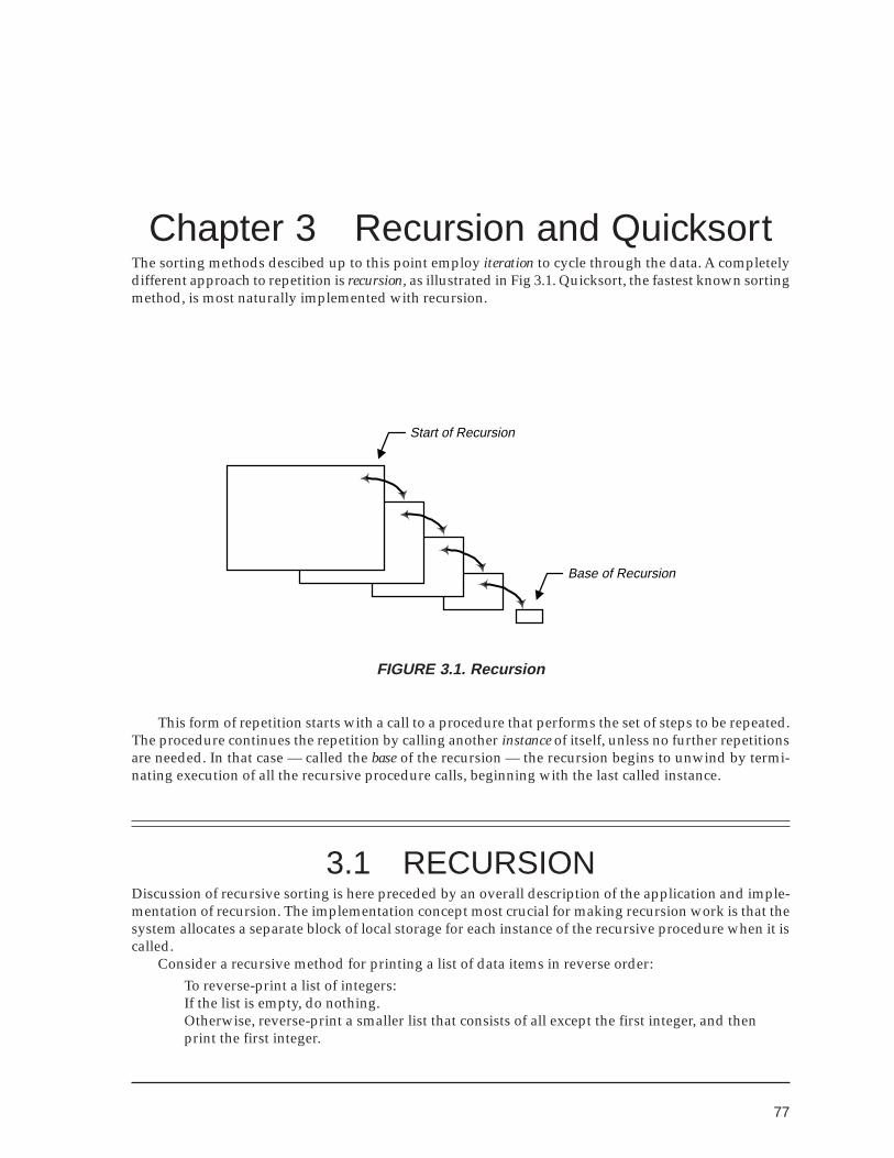
77
Chapter 3 Recursion and QuicksortThe sorting methods descibed up to this point employ iteration to cycle through the data. A completelydifferent approach to repetition is recursion, as illustrated in Fig 3.1. Quicksort, the fastest known sortingmethod, is most naturally implemented with recursion.
Start of Recursion
Base of Recursion
FIGURE 3.1. Recursion
This form of repetition starts with a call to a procedure that performs the set of steps to be repeated.The procedure continues the repetition by calling another instance of itself, unless no further repetitionsare needed. In that case — called the base of the recursion — the recursion begins to unwind by termi-nating execution of all the recursive procedure calls, beginning with the last called instance.
3.1 RECURSIONDiscussion of recursive sorting is here preceded by an overall description of the application and imple-mentation of recursion. The implementation concept most crucial for making recursion work is that thesystem allocates a separate block of local storage for each instance of the recursive procedure when it iscalled.
Consider a recursive method for printing a list of data items in reverse order:To reverse-print a list of integers:If the list is empty, do nothing.Otherwise, reverse-print a smaller list that consists of all except the first integer, and thenprint the first integer.
78
Some features of this description are common to many recursive problems:1. The method for performing a sequence of tasks (“reverse-print a list of integers”) is described quite
differently from the method for performing a component task (“print an integer”).
2. The way to perform a component task (“print an integer”) is supposed to be already known or to bedefined elsewhere.
3. The way to perform a sequence of tasks (“reverse-print a list”) is never completely specified; it isdescribed only incrementally — the procedure itself is composed from a derivative sequence of tasks(“reverse-print a smaller list”) and a component task (“print an integer”).
4. However, the performance of a certain base sequence (“reverse-print an empty list”) is describedcompletely.Recursive procedures should be created with some care. It is especially necessary to be sure that the
sequence of derivations generated at step 3 will eventually lead to the base. A very common class ofrecursive procedures involves an integer argument that decreases with each recursive call; with a smallinteger base, such as 1 or 0, eventual termination is assured.
The print application employs a slightly different strategy: It employs a list that grows shorter ateach derivation, with an empty list as the base. Suppose that the input file holds three integers, 101, 201,301, and 0, in this order. The zero is a “sentinel” value that is not considered part of the list; it merelyterminates the list and is not to be printed.
Reverse-print “101, 202, 303” by doing the following:Reverse-print “202, 303” by doing the following:
Reverse-print “303” by doing the following:Reverse-print “” (an empty list) by doing nothing;Print “303”.
Print “202”.Print “101”.
Stop.
Example 11. The following recursive procedure reads a data item and tests whether it is zero; if not,it calls itself recursively to read and process another item:
! Example 11. Reverse-print a list of integers.program D11
implicit none! start program D11
call Reverse_Print( )stop
containsrecursive subroutine Reverse_Print( )
integer :: A! start subroutine Reverse_Print
read *, A
Skip the recursive call when zero is read (the base case).
if (A /= 0) thencall Reverse_Print( )print *, A
end ifreturn
end subroutine Reverse_Print
end program D11
Recursion and Quicksort
79
The program declares only one variable, A, and yet it could apparently process an arbitrarily largenumber of data items. What happens to the earlier data items while later items are being read andprinted? As mentioned earlier, the crucial idea in the implementation of recursion is to give each in-stance of a recursive procedure its own activation record, which is a block of storage that contains aninstance of each local variable declared in the procedure.18 This block also contains procedure argu-ments (if any — in the form of values or references) for the current procedure instance, as well as infor-mation needed for returning to the reference point.
Let us examine the execution sequence for Reverse_Print in detail.• The main program calls Reverse_Print . Since there will be several instances of Reverse_Print ,
let us call the first one RP1.
• RP1 reads the integer 101 and assigns it to the variable A in the activation record for RP1, which wedesignate as “RP1’s A”. Since A is not zero, it calls Reverse_Print — i.e., RP2.
• RP2 reads 202 and assigns it to the variable A, this time designated as “RP2’s A”. Again A is not zeroso it calls Reverse_Print — i.e., RP3.
• RP3 reads 303 and assigns it to the variable “RP3’s A”. Again A is not zero so it calls RP4.
• RP4 reads 0 and assigns it to the variable “RP4’s A”. This time A is the sentinel which is not to beprocessed. RP4 makes no further procedure call and exits, thus returning control to RP3 at the pointjust after the call to RP4.
• RP3 continues by printing its copy of the variable A, namely “RP3’s A” which is 303. This is the firstnumber that has been printed during program execution up to this point. After the print step, RP3returns control to RP2 at the point just after the call to RP3.
• RP2 prints “RP2’s A”, which is 202, then returns control to RP1.
• RP1 prints “RP1’s A”, which is 101, then returns control to the main program and stops.
Recursion Compared with IterationSome problems can be described more naturally as recursive processes than as iterative processes. If younormally think of a factorial as an integer times a smaller factorial, you can translate that problem de-scription directly into a recursive program. On the other hand, recursion usually entails some loss inefficiency, including extra procedure-call overhead and hidden storage requirements.
This text recommends that program comprehension be viewed as the primary objective, givingsomewhat less importance to efficiency of execution. In the 1970s, emphasis on “structured program-ming” awakened computer users to the fact that small gains in efficiency can easily be lost due to errorsintroduced by failure to understand a problem.• Some applications can be viewed with almost equal ease either iteratively or recursively. Iteration is
always somewhat more efficient — it requires less overhead and less space — so iteration is prefer-able when there is no special reason to choose recursion.
• Some problems are very naturally understood with recursion and exceedingly awkward in iterativeform. Tree structures (see Chapter 7) are processed naturally by means of recursion, because a treeconsists of subtrees that have essentially the same structure as the tree itself. Quicksort (to be ex-plained next) depends naturally on recursion. Even in Fortran, such applications should not beforced into an unsuitable iterative form. Effort may be directed toward making the recursive versionas efficient as possible.
• Some applications require a more difficult choice between a recursive version that is a bit easier tounderstand and an iterative version that runs a bit faster or uses less storage. If efficiency is truly thedominant factor, iteration should be chosen. Otherwise, the recursive approach should be adopted
18 The activation record does not include variables with the save or allocatable attributes.
3.1 RECURSION
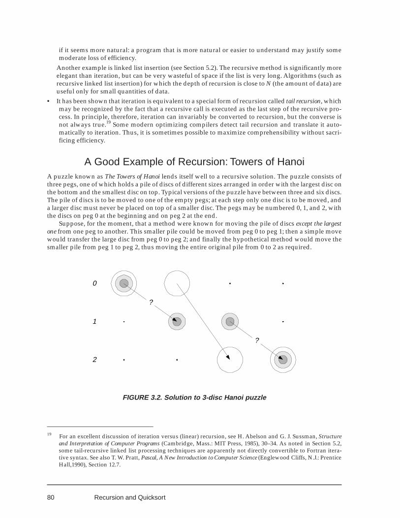
80
?
0
1
2
?
if it seems more natural: a program that is more natural or easier to understand may justify somemoderate loss of efficiency.
Another example is linked list insertion (see Section 5.2). The recursive method is significantly moreelegant than iteration, but can be very wasteful of space if the list is very long. Algorithms (such asrecursive linked list insertion) for which the depth of recursion is close to N (the amount of data) areuseful only for small quantities of data.
• It has been shown that iteration is equivalent to a special form of recursion called tail recursion, whichmay be recognized by the fact that a recursive call is executed as the last step of the recursive pro-cess. In principle, therefore, iteration can invariably be converted to recursion, but the converse isnot always true.19 Some modern optimizing compilers detect tail recursion and translate it auto-matically to iteration. Thus, it is sometimes possible to maximize comprehensibility without sacri-ficing efficiency.
A Good Example of Recursion: Towers of HanoiA puzzle known as The Towers of Hanoi lends itself well to a recursive solution. The puzzle consists ofthree pegs, one of which holds a pile of discs of different sizes arranged in order with the largest disc onthe bottom and the smallest disc on top. Typical versions of the puzzle have between three and six discs.The pile of discs is to be moved to one of the empty pegs; at each step only one disc is to be moved, anda larger disc must never be placed on top of a smaller disc. The pegs may be numbered 0, 1, and 2, withthe discs on peg 0 at the beginning and on peg 2 at the end.
Suppose, for the moment, that a method were known for moving the pile of discs except the largestone from one peg to another. This smaller pile could be moved from peg 0 to peg 1; then a simple movewould transfer the large disc from peg 0 to peg 2; and finally the hypothetical method would move thesmaller pile from peg 1 to peg 2, thus moving the entire original pile from 0 to 2 as required.
19 For an excellent discussion of iteration versus (linear) recursion, see H. Abelson and G. J. Sussman, Structureand Interpretation of Computer Programs (Cambridge, Mass.: MIT Press, 1985), 30–34. As noted in Section 5.2,some tail-recursive linked list processing techniques are apparently not directly convertible to Fortran itera-tive syntax. See also T. W. Pratt, Pascal, A New Introduction to Computer Science (Englewood Cliffs, N.J.: PrenticeHall,1990), Section 12.7.
Recursion and Quicksort
FIGURE 3.2. Solution to 3-disc Hanoi puzzle
81
Like the reverse-print procedure, the foregoing paragraph never completely tells how to “move apile of discs”; it describes only a similar but simpler task (“move all of the discs except the largest one”)and a component task (“transfer the largest disc”):To move n discs from peg i to peg j:
• If n is 1, simply transfer the single disc from peg i to peg j;
• Otherwise, move n – 1 discs (all except the largest) from peg i to peg k (the peg that is neither i nor j),transfer the largest disc from peg i to peg j, and move n – 1 discs from peg k to peg j.For a more complicated iterative solution, place the pegs at the vertices of an equilateral triangle
and alternate between moving the smallest disc clockwise and moving the only other available disccounterclockwise.
The number of moves for n discs is 2n – 1. As we shall see in the following chapter, this algorithm isunfeasible if n is large. However, an algorithm that simulates each of the individual moves will unavoid-ably require an amount of calculation approximately proportional to 2n. The size of the task is inherentin the problem, and not in the method of solution. The recursive solution seems to give more insight intothe problem than the iterative version.
A Bad Example of Recursion: The Fibonacci SequenceAbout 800 years ago Leonard of Pisa, surnamed Fibonacci, posed the following problem: “A certain manput a pair of rabbits in a place surrounded by a wall. How many pairs of rabbits can be produced fromthat pair in a year, if it is supposed that every month each pair begets a new pair which from the secondmonth on becomes productive?” The number of pairs each month is given by the Fibonacci sequence 1, 1,2, 3, 5, 8, 13, 21, 34, 55, 89, 144, . . ., in which each number after the first two is the sum of the two previousnumbers:
pure recursive function Fibonacci( N ) result( Fibonacci_R )integer, intent(in) :: Ninteger :: Fibonacci_R
! start function Fibonacciif (N <= 2) then
Fibonacci_R = 1else
Fibonacci_R = Fibonacci( N - 1) + Fibonacci(N - 2 )end ifreturn
end function Fibonacci
This recursive function produces the correct result so long as N is small enough. For the result to berepresentable as a 4-byte IEEE integer, N must not exceed 46; however, the procedure is intolerably slowfor values of N near the upper end of this range. Each call to the function with N > 2 generates two morecalls to the same function; the total number of recursive function calls is the same as the result beingcalculated: approximately 1.6N calls, or more than 107 (46 seconds on our benchmark machine) for N =36, 108 (almost nine minutes) for N = 41, and 109 function calls (more than 1.5 hours) for N = 46.
Much simpler methods are available. Fibonacci numbers can be calculated iteratively by a methodwhose running time is linear in N. The following steps begin with the first two Fibonacci numbers, bothof which are 1. The two previous values are saved at each step.
3.1 RECURSION
82
Fibonacci_R = 1if( N > 2) then
Prev_1 = 1do Loop = 3, N
Prev_2 = Prev_1Prev_1 = Fibonacci_RFibonacci_R = Prev_1 + Prev_2
end doend if
Still more simply (and with constant running time, independent of N), the Nth Fibonacci number canbe calculated directly from the formula (αN – βN)/(α – β), where α and β are roots of the quadraticequation x2 – x – 1 = 0; namely, (1 ± √5) / 2 , i.e., 1.618033989 and −0.618033989 . With IEEE eight-byte realrepresentation, this formula gives correct results (to the nearest integer) for N ≤ 46.
! Fibonacci numbers by direct calculation from formulaprogram Fibonacci
integer, parameter :: SRK9 = selected_real_kind( 9 )real(kind = SRK9), parameter :: ALFA = 1.618033988749895_SRK9, &
BETA = - 0.618033988749895_SRK9, &DELTA = 2.23606797749978969641_SRK9
integer :: N! start program Fibonacci
doprint *, " Please enter an integer between 0 and 46"print *, " Enter an integer larger than 46 to stop."read *, Nif ((N < 0) .or. (N > 46)) stopwrite (*, "( t2, i4, f20.0 )") N, (ALFA ** N - BETA ** N) / DELTA
end dostop
end program Fibonacci
Since β is smaller than 1, it turns out that βN can be ignored if the “nearest integer” function is applied:write (*, "( t2, i4, i24.0 )") N, nint( ALFA ** N / DELTA )
Application: Adaptive Quadrature (Numerical Integration)
Example 12. A numerical application that employs recursion is adaptive quadrature. A one-stepSimpson Rule calculation is applied to the whole interval (A, B); the result is compared with the sum ofone-step calculations applied separately to the left and right halves of the interval. If these are nearlyequal, the sum is accepted as the final answer; otherwise, adaptive quadrature is applied recursively toeach half interval. The effect is to apply smaller step sizes where the integrand has greater functionalvariation. It has been pointed out that this technique is successful for most problems because each sub-division typically decreases the approximation error by a factor of 15 but tightens the accuracy require-ment by only a factor of two.20 (For Fortran 95 versions, which declare Quad as a pure function, theintegrand Func must also be a pure function. See also the electronic examples, in which the integrandis implemented as a dummy procedure.)
Recursion and Quicksort
20 R. L. Burden and J. D. Faires, Numerical Analysis, th ed. (Boston: PWS Publishing, )
83
! Example 12. Adaptive Quadrature (Numerical Integration)
:integer, parameter, public :: HI = selected_real_kind( 12 )type, public :: Result_Type
real(kind = HI) :: X, Err_Loclogical :: Error
end type Result_Type:
recursive pure function Quad(A, B, I, Tol, M_Int ) result( Quad_R )real(kind = HI), intent (in) :: A, B, I, Tol, M_Inttype(Result_Type) :: Quad_Rtype(Result_Type) :: R1, R2real(kind = HI) :: Y, Z, M
! start function QuadM = (A + B) / 2.0_HIY = Simpson( A, M )Z = Simpson( M, B )if (abs( Y + Z - I ) > Tol) then
if (abs( B - A ) < M_Int) then ! Not OK but interval is too smallQuad_R = Result_Type( I, M, .true. )
else ! Not OK: Subdivide interval againR1 = Quad( A, M, Y, Tol / 2.0_HI, M_Int )R2 = Quad( M, B, Z, Tol / 2.0_HI, M_Int )Quad_R % X = R1 % X + R2 % XQuad_R % Error = R1 % Error .or. R2 % Errorif (Quad_R % Error) then
Quad_R % Err_Loc = merge(R1 % Err_Loc, R2 % Err_Loc, R1 % Error)end if
end ifelse ! OK: Accept current value.
Quad_R = Result_Type( Y + Z, M, .false. )end ifreturn
end function Quad
pure function Simpson( A, B ) result( Simpson_R )real (kind = HI), intent(in) :: A, Breal (kind = HI) :: Simpson_Rreal (kind = HI) :: M
! start function SimpsonM = (A + B) / 2.0_HISimpson_R = (B - A) * (Func( A ) + 4.0_HI * Func( M ) + Func( B )) / 6.0_HIreturn
end function Simpson
3.1 RECURSION
84
Application: Recursive Selection SortThe selection sort method is easy to describe as a recursive algorithm: If there is more than one item tosort, find the largest item, swap it with the last item, and then apply the selection sort algorithm toeverything else.
module Recursive_Selectuse Swap_Reals_Mimplicit noneprivatepublic :: Selection_Sort
containsrecursive subroutine Selection_Sort( Unsorted ) ! Module subprogram
real, dimension(:), intent (in out) :: Unsortedinteger :: Ninteger, dimension(1) :: Loc
! start subroutine Selection_SortN = Size( Unsorted )if (N > 1) then ! End recursion if only one element remains.
Loc = maxlLoc( Unsorted ) ! Location of largest elementcall Swap( Unsorted(N), Unsorted(Loc(1)) )call Selection_Sort( Unsorted(1: N - 1) ) ! Recursion
end ifreturn
end subroutine Selection_Sortend module Recursive_Select
Tail Recursion vs Iteration
Printing a List Forward
Consider a recursive method for printing a list of data items in forward order:To forward-print a list of integers:If the list is empty, do nothing.
Otherwise, print the first integer, and then forward-print the remainder of the list (consisting of theoriginal list except for the first integer).
recursive subroutine Forward_Print( )integer :: A
! start subroutine Forward_Printread *, A
Skip the recursive call when zero is read (the base case).
if (A /= 0) thenprint *, Acall Forward_Print( )
end ifreturn
end subroutine Forward_Print

85
This recursive algorithm has the special form mentioned earlier (a recursive call is executed as its laststep) so it can be converted to an iterative procedure. The recursive call can simply be changed to a goto statement, as follows:
1 read *, Aif (A /= 0) then
print *, Ago to 1
end ifBetter programming style would be the equivalent do construct:
subroutine Forward_Print( ) ! iterative, with do constructinteger :: A
! start subroutine Forward_Printdo
read *, Aif (A == 0) then
exitelse
print *, Aend if
end doreturn
end subroutine Forward_Print
Factorial
Viewed recursively, the factorial of a nonnegative integer n is n times the factorial of n – 1; the factorial ofzero is 1:
pure recursive function Factorial( N ) result( Factorial_R )integer :: Factorial_R
! start function Factorialif (N < 1) then
Factorial_R = 1else
Factorial_R = N * Factorial( N - 1 )end ifreturn
end function Factorial
The procedure call overhead of this tail-recursive implementation makes it terribly inefficient, ascompared to iteration (except with optimizers that perform the conversion automatically). See Exercise2 below. However, if you view the recursive definition as more natural, and if efficiency is not especiallyimportant, you might still prefer this version. Anyway, on typical hardware the factorial function isrepresentable as an ordinary integer only for quite small values of N: for example, the factorial of 13 istoo large to be represented as an IEEE 4-byte integer.
Section 3.1 Exercises1. Write a recursive subroutine that simulates the moves in a Towers of Hanoi puzzle, and prints each
move. Subroutine dummy arguments are n, i, and j. (Hint: set k to 3 – (i + j).) Write a main programthat calls the subroutine with n = 4, i = 0, j = 1.
2. Write an iterative factorial function with a do construct.
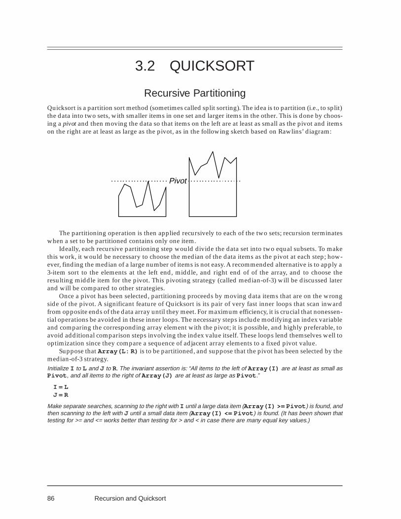
86
Pivot
3.2 QUICKSORT
Recursive PartitioningQuicksort is a partition sort method (sometimes called split sorting). The idea is to partition (i.e., to split)the data into two sets, with smaller items in one set and larger items in the other. This is done by choos-ing a pivot and then moving the data so that items on the left are at least as small as the pivot and itemson the right are at least as large as the pivot, as in the following sketch based on Rawlins’ diagram:
Recursion and Quicksort
The partitioning operation is then applied recursively to each of the two sets; recursion terminateswhen a set to be partitioned contains only one item.
Ideally, each recursive partitioning step would divide the data set into two equal subsets. To makethis work, it would be necessary to choose the median of the data items as the pivot at each step; how-ever, finding the median of a large number of items is not easy. A recommended alternative is to apply a3-item sort to the elements at the left end, middle, and right end of of the array, and to choose theresulting middle item for the pivot. This pivoting strategy (called median-of-3) will be discussed laterand will be compared to other strategies.
Once a pivot has been selected, partitioning proceeds by moving data items that are on the wrongside of the pivot. A significant feature of Quicksort is its pair of very fast inner loops that scan inwardfrom opposite ends of the data array until they meet. For maximum efficiency, it is crucial that nonessen-tial operations be avoided in these inner loops. The necessary steps include modifying an index variableand comparing the corresponding array element with the pivot; it is possible, and highly preferable, toavoid additional comparison steps involving the index value itself. These loops lend themselves well tooptimization since they compare a sequence of adjacent array elements to a fixed pivot value.
Suppose that Array(L: R) is to be partitioned, and suppose that the pivot has been selected by themedian-of-3 strategy.Initialize I to L and J to R. The invariant assertion is: “All items to the left of Array(I) are at least as small asPivot , and all items to the right of Array(J) are at least as large as Pivot .”
I = LJ = R
Make separate searches, scanning to the right with I until a large data item (Array(I) >= Pivot ) is found, andthen scanning to the left with J until a small data item (Array(I) <= Pivot ) is found. (It has been shown thattesting for >= and <= works better than testing for > and < in case there are many equal key values.)
87
dodo
I = I + 1if (Array(I) >= Pivot) exit
end dodo
J = J - 1if (Array(J) <= Pivot) exit
end do
If the two scans have met or crossed, this partition is complete. Otherwise, swap the large and small data items andcontinue scanning to the right with I and to the left with J .
if (I >= J) exitcall Swap( I, J )
end docall Recursive_QS( L, J )call Recursive_QS( J + 1, R )
Here is an example. S O R T M E Q U I C K L Y
A 3-item sort is applied to S, Q, and Y, thus changing S Q Y to Q S Y, and S (the median of these threeitems) is chosen as the Pivot. The scans begin moving inward from each end.
Q> O R T M E S U I C K L <Y
Starting from the left end and moving toward the right, T is the first item that is at least as large as S;starting from the right end and moving toward the left, L is the first item that is at least as small as S.These two items are swapped; then the inward scans continue, comparing the items that remain be-tween the two that were swapped.
Q O R L> M E S U I C K <T Y
Moving right, S is at least as large as S; moving left, K is at least as small as S. Therefore, S and K areswapped, and the scans continue.
Q O R L M E K> U I C <S T Y
Moving right, U is at least as large as than S; moving left, C is at least as small as S. After U and C areswapped, the scans continue.
Q O R L M E K C> I <U S T Y
Moving right, U is again at least as large as S; moving left, I is at least as small as S. The scans have nowcrossed, so no swap occurs.
Q O R L M E K C <I U> S T Y
This partition is now complete. The first nine items are at least as small as S, and the last four items areat least as large as S. Note that the pivot does not necessarily end up adjacent to the partition.
Q O R L M E K C I# U S T Y
Recursively, each of the two groups is now partitioned. Consider the first group of nine items. Thescans begin after Q, M, and I have been sorted and M has been chosen as the Pivot.
I> O R L M E K C <Q
Moving right, O is at least as large as M; moving left, C is at least as small as M. These two items areswapped and the scans continue.
I C> R L M E K <O Q
Moving right, R is at least as large as M; moving left, K is at least as small as M. These two items areswapped and the scans continue.
I C K> L M E <R O Q
3.2 QUICKSORT
88
Moving right, M is at least as large as M; moving left, E is at least as small as M, so M and E are swappedand the scans continue.
I C K L E> <M R O Q
Moving right, M is at least as large as M; moving left, E is at least as small as M. The scans have nowcrossed, so no swap occurs.
I C K L <E M> R O Q
The first five items are at least as small as M, and the last four items are at least as large as E. I C K L E# M R O Q
Quicksort continues, recursively partitioning each of these two groups.
Quicksort is Unstable for Duplicates
It is easy to see that quicksort is unstable for duplicate items. (Here, subscripts are shown only foridentification and are not part of the key.) The pivot for the first partition is E1:
A1 B1 C1 D1 E1 A2 B2 C2 D2 E2 A1> B1 C1 D1 E1 A2 B2 C2 D2 <E2 A1 B1 C1 D1 D2> A2 B2 C2 <E1 E2 A1 B1 C1 D1 D2 A2 B2 <C2 E1> E2 A1 B1 C1 D1 D2 A2 B2 C2# E1 E2
For positions 1 to 8, the pivot is C2: A1 B1 C1 D1 D2 A2 B2 C2 A1> B1 C1 C2 D2 A2 B2 <D1 A1 B1 B2> C2 D2 A2 <C1 D1 A1 B1 B2 A2> D2 <C2 C1 D1 A1 B1 B2 <A2 D2> C2 C1 D1 A1 B1 B2 A2# D2 C2 C1 D1
For positions 1 to 4, the pivot is A2: A1 B1 B2 A2 A1> A2 B2 <B1 A1 <A2> B2 B1 A1 A2# B2 B1
For positions 1 to 2, the pivot is A1: A1 A2 A1> <A2<A1 A2> A1# A2
For positions 3 to 4, the pivot is B2: B2 B1 B2> <B1<B2 B1> B2# B1
For positions 5 to 8, the pivot is D2:
Recursion and Quicksort
89
D2 C2 C1 D1 C2> D2 C1 <D1 C2 C1> <D2 D1 C2 <C1 D2> D1 C2 C1# D2 D1
For positions 5 to 6, the pivot is C2: C2 C1 C2> <C1<C2 C1> C2# C1
For positions 7 to 8, the pivot is D2: D2 D1 D2> <D1<D2 D1> D2# D1
For positions 9 to 10, the pivot is E1: E1 E2 E1> <E2<E1 E2> E1# E2
The final sorted array appears as follows: A1 A2 B2 B1 C2 C1 D2 D1 E1 E2
Choosing the Pivot
Properly implemented, quicksort is the fastest known sorting algorithm. However, as Sedgewick21 pointsout, the algorithm is “fragile”: small changes in some of the program steps can destroy the efficiency ofthe method or can lead to undesirable and unexpected effects for some inputs.
“Once a version has been developed and seems free of such effects, this is likely to be the program touse for a library sort or for a serious sorting application. But [one must be] willing to invest the effortto be sure that a quicksort implementation is not flawed. . . .”One change that can have dramatic effects relates to the choice of a pivot element for each partition.
As stated earlier, the ideal pivot would be the median of the data items, so that the partitioning processwould produce equal subgroups. However, the extra time required to find the true median would de-stroy the fast performance of quicksort.
Some published quicksort algorithms choose a specific array element, such as ArrayL or ArrayL+R/2,as the pivot. Others generate a random subscript value between L and R.
Warnock22 suggests using the median-of-3 pivot strategy mentioned earler, based on the first andlast items and an item between them chosen at random. A random array element can be selected withthe intrinsic subroutine random_number :
call random_number( X )C = L + int( X * real( R - L ) )call Sort_3( L, C, R )Pivot = Array(C)
21 Sedgewick, Algorithms, 116.22 Private communication
3.2 QUICKSORT

90
Use of the actual median of a tiny sample of the data tends to equalize the partitions somewhat.23 Ithas the additional advantage that a bit of the sorting is done along with the pivot choice, so the scan canomit the item at each end — for most other strategies, the elements at each end are not examined beforethe scans begin, so I must be initialized to L – 1 and and J to R + 1. Furthermore, median-of-3 pivotingguarantees that both inner loops will exit without running off the ends of the array; other strategies mayrequire extra steps to avoid disaster. (The index values could be tested in the inner loop, of course, butthis would dramatically increase the total sort time.)
The Cutoff
One variation of quicksort can significantly improve the performance of the algorithm. Quicksort is veryeffective for large amounts of data but is not especially fast for sorting fewer than a dozen items. Fur-thermore, sorting small groups of items by quicksort requires several recursive calls and thus introducesa disproportionate amount of overhead.
A quicksort implementation may specify a cutoff value to avoid recursively processing small sets,i.e., sets for which the difference between right end and left end subscripts does not exceed the cutoff. Inthe algorithms presented here, small sets are left unsorted and a final pass is made over the whole arraywith straight insertion, taking advantage of the efficiency of this latter method for data that is nearly inorder.24
The optimum cutoff value depends somewhat on hardware characteristics. Some experimentationusually reveals a very shallow minimum, with any cutoff from about 5 to 20 giving an improvementbetween 5% and 15%, even after taking into account the extra time required for the final insertion sort.
Testing a Quicksort ImplementationAt least three tests should be made to improve confidence in an implementation of quicksort.1. Sequence check. It goes without saying that the data should be in order after it has been processed by
quicksort.
2. Timing comparison with insertion sort. Many implementations of quicksort end with a straight inser-tion pass, so a quicksort procedure that is not working at all will produce a correct data sequence ifthe insertion sort is implemeted correctly. For about 10,000 random data items, a correct quicksortprocedure is at least 100 times as fast as insertion. If your procedure is only slightly faster thaninsertion, most of the work is being done during the final insertion pass.
3. Asymptotic running time. Quicksort should be applied to several large sets of random data of differ-ent sizes — for example, 100,000 items and one million items. The elapsed time ratio should verifythe N lg N asymptotic behavior that is characteristic of quicksort: One million items should takebetween 10 and 15 times as long as 100,000 items.
23 According to Moret and Shapiro (B. M. E. Moret and H. D. Shapiro, Algorithms from P to NP, Redwood City CA:Benjamin/Cummings, 1990, 516), consistently choosing any specific element as the pivot (or choosing thepivot at random) results in an expected split of 25:75; the median-of-3 strategy gives an expected split close to33:67 and reduces the probability of a 25:75 or worse split to about 0.3.
A strategy sometimes suggested is simply to use the leftmost data array element as the pivot. However, if thismethod is applied to a set of data that happens to be in order (or in reverse order) already, each group of kitems will be partitioned into a single item and a group of k – 1 items. The method is nearly as bad for data thatis almost in order: quicksort becomes merely an inefficient recursive version of selection sort. Since sortingalgorithms are often applied to data that is nearly in order, the effect of this bad pivot choice is “quite embar-rassing,” to quote Knuth.
24 In a paged environment, it may be preferable to sort the small sets by insertion or selection as they are created,as Moret and Shapiro note: “This strategy preserves the excellent locality of quicksort, whereas the final sweepof a single insertion sort pass would trigger another series of page faults.”
Recursion and Quicksort
91
Storage Space ConsiderationsWhen a procedure with an array argument calls itself recursively, does each instance of the procedurestore another copy of the array? Probably not — array arguments are almost invariably passed by refer-ence, so each instance stores only an address. For Fortran assumed-shape arrays this is a reference to thearray descriptor.
It is not difficult to entirely eliminate the array argument from a recursive procedure. A nonrecursive“wrapper” procedure with an array argument is constructed, with the recursive procedure as an inter-nal procedure inside it. The recursive procedure inherits the original array from the wrapper and hasonly two integer scalar arguments, the left and right end index values. A less flexible alternative thateliminates the wrapper (and, perhaps surprisingly, seems to run almost twice as fast on some systems)declares a public data array in the module where the recursive sort is defined. (The F subset does notsupport internal procedures; the nonrecursive wrapper and the recursive procedure are module proce-dures at the same level, so the recursive procedure can inherit only from the specification part of themodule. A public array may be employed as just described, or the array may be passed as an argumentto the wrapper and then copied to a private array declared at the module level.)
For ideal partitioning (and with zero cutoff), the maximum depth of recursion would be lg N. Ex-periments with random data and with the median-of-3 pivot strategy find a maximum recursive depthonly slightly greater than lg N, but it can be 2 to 3 times this large — in one test with a million items (lgN = 20) and cutoff 16, the maximum depth reached 52 levels of recursion. However, the extra recursivelevels do not consume much space because the activation record for each instance needs to store onlytwo scalar integer arguments (the endpoint index values L and R), a local variable for the partition pointJ, and a few items of system information — a few hundred extra bytes altogether for a million dataitems. The following implementation employs three additional local variables, I, C, and Pivot; to mini-mize local storage space in the recursive procedure, these three variables may be moved to the wrappersubroutine or to the specification part of the containing module.25
Say It with Fortran
Example 13.
! Example 13. Quicksort
Nonrecursive “wrapper”
subroutine Qu_Sort( Array )real, dimension(:), intent(in out) :: Arrayinteger :: N
! start subroutine Qu_SortN = size( Array )call Recursive_QS( 1, N )if (CUT_OFF > 0) call In_Sort( )return
contains
3.2 QUICKSORT
25 If very deep recursion occurs due to unusual data characteristics, the endpoints of the larger partition may bepushed on a user-defined stack and the smaller partition processed iteratively. As Moret and Shapiro note (p.516), this technique insures that the stack does not contain more than lg N entries. Sedgewick (p. 122) gives aPascal implementation of this iterative (pseudo-recursive) version.
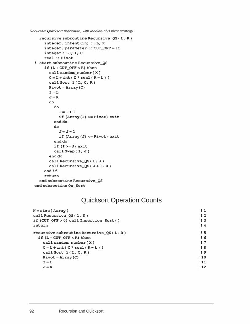
92
Recursive Quicksort procedure, with Median-of-3 pivot strategy
recursive subroutine Recursive_QS( L, R )integer, intent(in) :: L, Rinteger, parameter :: CUT_OFF = 12integer :: J, I, Creal :: Pivot
! start subroutine Recursive_QSif (L + CUT_OFF < R) then
call random_number( X )C = L + int( X * real( R - L ) )call Sort_3( L, C, R )Pivot = Array(C)I = LJ = Rdo
doI = I + 1if (Array(I) >= Pivot) exit
end dodo
J = J - 1if (Array(J) <= Pivot) exit
end doif (I >= J) exitcall Swap( I, J )
end docall Recursive_QS( L, J )call Recursive_QS( J + 1, R )
end ifreturn
end subroutine Recursive_QSend subroutine Qu_Sort
Quicksort Operation Counts
N = size( Array ) ! 1call Recursive_QS( 1, N ) ! 2if (CUT_OFF > 0) call Insertion_Sort( ) ! 3return ! 4
recursive subroutine Recursive_QS( L, R ) ! 5if (L + CUT_OFF < R) then ! 6
call random_number( X ) ! 7C = L + int( X * real( R - L ) ) ! 8call Sort_3( L, C, R ) ! 9Pivot = Array(C) ! 10I = L ! 11J = R ! 12
Recursion and Quicksort
93
do ! 13do ! < 14
I = I + 1 ! << 15if (Array(I) >= Pivot) exit ! << 16
end do ! << 17do ! < 18
J = J - 1 ! << 19if (Array(J) <= Pivot) exit ! << 20
end do ! << 21if (I >= J) exit ! < 22call Swap( I, J ) ! 23
end do ! 24call Recursive_QS( L, J ) ! 25call Recursive_QS( J + 1, R ) ! 26
end if ! 27
Sort_3 uses 3 comparisons and 4.5 moves (but sorting the three items by insertion can decrease thesecounts slightly). An estimate for the outer loop (lines 13 – 24) is 0.25·N iterations, with each inner loopiterating twice. Each iteration of the outer loop body performs 4 data item comparisons (2 in each innerloop) and one swap (3 move operations) almost always. Thus lines 13 – 24 require N comparisons and0.75·N moves; the total for lines 1– 24 (ignoring the call to random_number ) is N + 3 comparisons and0.75·N + 4.5 moves.
For a recursive procedure, the operation count formula for a given number of items often dependsupon the same formula applied to a smaller number of items — that is, it must be expressed as a recur-rence relation. The operation count for lines 25 and 26 has the form TN = A + B·N + TJ+1–L + TR–J, where Tis either the number of comparisons or the number of moves. For the case of ideal partitioning, TJ+1–L andTR–J are nearly equal so that TN = A +B·N +2 TN/2. Moret and Shapiro26 show how to solve such recurrencerelations, by difference equation methods that are similar to well-known methods for initial value prob-lems in differential equations, to obtain a closed-form formula for TN. In this case, if N is a power of 2 thesolution with T(1) = 0 is TN = B·N lg N +A·(N – 1). Although the solution of recurrences is beyond thescope of this text, Section 4.3 shows how to use mathematical induction to show consistency between arecurrence relation and the derived closed-form formula.
For comparison operations, A is 3 and B is 1 giving CN = N lg N +3·N – 3; for move operations, A is 4.5and B is 0.75 giving MN = 0.75·N lg N +4.5·N – 4.5
A benchmark, run with a 50 MHz 486DX computer, sorted one million random real numbers in 56seconds, with median-of-3 pivot strategy and cutoff 12.• Quicksort
The worst-case operation count is proportional to N2, but median-of-3 pivot strategy with themiddle element chosen at random makes the worst case extremely unlikely. A “cutoff” valuebetween 5 and 20 is recommended, with a final straight insertion sort.Comparisons: N lg N +3·N – 3Moves: 0.75 N lg N +4.5·N – 4.5Benchmark time for 1 million random real numbers: 56 seconds
3.3 QUICKSORT OPERATION COUNTS
26 Algorithms from P to NP, 61-81. The substitution K = lg N converts the recurrence to S(K) = A +B·2K + 2·S(K -1);S(0) = 0. See also Sedgewick, Algorithms, 77.
94
Chapter 4 Algorithm Analysis
4.1 WHAT IS AN ALGORITHM?The sorting methods described in Chapter 2 are examples of algorithms — each is a sequence of stepsfor accomplishing a specific task. There is an important difference between an algorithm and a com-puter program: The algorithm describes the general method for performing a task, without regard to thedetails of its implementation. In principle, a given algorithm should be capable of implementation inany of several computer languages, or even by some other means without using a computer at all. Anexample of an algorithm that would usually be implemented without a computer is a recipe for bakingapple pie, which is a description of the sequence of steps that are required to perform this specific task.
To constitute an algorithm, a sequence of steps should have the following properties:1. The steps in an algorithm must not be too big nor too small. The size of an appropriate step depends
upon the executor of the algorithm, which could be a machine, a person, a trained chimpanzee, orwhatever. Each step should be the right size for the executor to perceive as a single unit of work.
An apple pie recipe in an old-fashioned cookbook consists of instructions appropriate for some-one with a reasonable amount of experience as a baker of pies. A cookbook for a sixth grade cookingclass would be much more detailed, while a baker with many years’ experience might require onlyone or two notes.
2. An algorithm must be finite: the list of steps must be finite in length, and its execution sequencemust eventually terminate. If some of the steps will be repeated (iteratively or recursively), therepetition must be guaranteed to terminate and not to continue forever. For some algorithms, progresstoward completion can be measured by an integer — for example, the selection sort algorithm re-moves one item from the unsorted sequence at each step, so the number of unsorted items willeventually reach zero.
3. Each step of an algorithm must be definite. That is, the executor must know precisely what to do ateach point. The steps are not strictly required to be deterministic; some algorithms, such as one forcounting “heads” in a sequence of coin tosses, may incorporate random elements. But the executormust know precisely how to proceed in any possible situation; for example, how to toss the coin,how to decide whether it is “heads,” and how to accumulate the count value.Most useful algorithms have some degree of generality — they are adaptable for solving any one
task from a class of related tasks. For example, a general sorting algorithm can be applied to any numberof items.
Computer AlgorithmsWhen an algorithm is to be executed by a computer, it must be expressed in steps each of which can beundertaken as a unit. An algorithm may be written initially in pseudocode, i.e., as a list human-readablestatements that cannot be interpreted directly by the computer but can easily be transformed into any ofseveral programming langauges such as Fortran, C++, or Pascal.
95
Some of the pseudocode steps — for example, “add a given item to the end of the sorted sequence” —will correspond to a single statement in Fortran. Others, such as “find the smallest unsorted item,” maybecome a procedure that consists of several Fortran statements.
Ultimately, the actual computer hardware executes the algorithm as a sequence of machine-lan-guage instructions that the compiler generates from the program statements.
4.2 WHAT MAKES A GOOD ALGORITHM?For most applications that are implemented with Fortran, speed of execution is a primary objective.Fortran compilers perform many extensive and sophisticated optimizations, such as detecting programstatements that can be moved out of a loop. For example, suppose that the selection sort procedure werewritten as follows:
do I = 1, size( Array ) - 1Location = Minimum_Location( I, size( Array ) )call Swap( I, Location )
end do
An optimizing compiler might recognize that the statements as written call for repeated execution of theintrinsic function reference
size( Array )(in the actual argument list for Minimum_Location ) at every iteration of the loop, even though thesame result value is returned at every reference. This expression can be evaluated once before the loopbegins, instead of once for every iteration of the loop; moving this statement would save a total of N – 2calls to the intrinsic function size . (Bill Long observes that no reasonable compiler would need to makean actual procedure reference to determine the size of an array — even one that is dynamically allo-cated. Nevertheless, we proceed with the example for purposes of hypothetical illustration.)
For sorting 1,000 items by selection, the optimization saves almost 1,000 intrinsic function calls.The 50 MHz processor of our estimates performs the sort in about 1 second; the optimization savesperhaps 200 microseconds or less than 0.2%. On the other hand, sorting the same 1,000 items by binaryinsertion takes about 0.19 second and thus saves about 80%; quicksort takes 0.03 second and saves 97%.
Moral: There may be more gain from choosing a suitable algorithm than from cleverly optimizingan unsuitable one. Choice of a suitable algorithm can have an even greater effect for larger amounts ofdata.
Relative speed is not the only criterion for judging algorithms, however.Another traditional criterion is the storage space required. Although this factor seems less impor-
tant in a typical modern computing environment, there are some scientific applications (such as hydro-dynamics calculations involved in weather research or in simulations of the effects of explosives) forwhich space availability significantly affects the precision of the results. Modern utility software such asoperating systems, word processors, spreadsheets, and database systems is often space limited, so spaceeconomy is an important criterion for the sorting, searching, and similar algorithms that are imbeddedin this software.
Other criteria that are harder to measure can be at least as important in the long run. In a choicebetween two algorithms, one of them might be easier to understand, to code, to debug, and to maintain;or one might be less dependent on properties of a particular operating environment and hence moreportable; or one might be more robust — i.e., less likely to have difficulty in the face of unexpectedcircumstances such as improper input data. Differences like these should often be weighted ahead ofslight improvements (say 10 percent) in speed.
Sorting is a good introductory subject for the study of algorithm efficiency, both because the subjecthas been extensively studied and because it has many practical applications. This text covers several ofthe best-known and most useful sorting algorithms.
4.2 WHAT MAKES A GOOD ALGORITHM
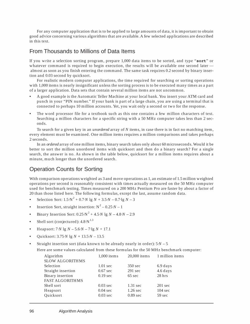
96
For any computer application that is to be applied to large amounts of data, it is important to obtaingood advice concerning various algorithms that are available. A few selected applications are describedin this text.
From Thousands to Millions of Data Items
If you write a selection sorting program, prepare 1,000 data items to be sorted, and type “sort ” orwhatever command is required to begin execution, the results will be available one second later —almost as soon as you finish entering the command. The same task requires 0.2 second by binary inser-tion and 0.03 second by quicksort.
For realistic modern computer applications, the time required for searching or sorting operationswith 1,000 items is nearly insignificant unless the sorting process is to be executed many times as a partof a larger application. Data sets that contain several million items are not uncommon.• A good example is the Automatic Teller Machine at your local bank. You insert your ATM card and
punch in your “PIN number.” If your bank is part of a large chain, you are using a terminal that isconnected to perhaps 10 million accounts. Yet, you wait only a second or two for the response.
• The word processor file for a textbook such as this one contains a few million characters of text.Searching a million characters for a specific string with a 50 MHz computer takes less than 2 sec-onds.To search for a given key in an unordered array of N items, in case there is in fact no matching item,
every element must be examined. One million items requires a million comparisons and takes perhaps2 seconds.
In an ordered array of one million items, binary search takes only about 60 microseconds. Would it bebetter to sort the million unordered items with quicksort and then do a binary search? For a singlesearch, the answer is no. As shown in the table below, quicksort for a million items requires about aminute, much longer than the unordered search.
Operation Counts for Sorting
With comparison operations weighted as 3 and move operations as 1, an estimate of 1.5 million weightedoperations per second is reasonably consistent with times actually measured on the 50 MHz computerused for benchmark testing. Times measured on a 200 MHz Pentium Pro are faster by about a factor of20 than those listed here. The following formulas, except the last, assume random data.• Selection Sort: 1.5·N2 + 0.7·N lg N + 3.5·N – 0.7·lg N – 3
• Insertion Sort, straight insertion: N2 – 0.25·N – 1
• Binary Insertion Sort: 0.25·N2 + 4.5·N lg N – 4.8·N – 2.9
• Shell sort (conjectured): 4.8·N1.3
• Heapsort: 7·N lg N – 5.6·N – 7·lg N + 17.1
• Quicksort: 3.75·N lg N + 13.5·N – 13.5
• Straight insertion sort (data known to be already nearly in order): 5·N – 5Here are some values calculated from these formulas for the 50 MHz benchmark computer:
Algorithm 1,000 items 20,000 items 1 million itemsSLOW ALGORITHMSSelection 1.01 sec 350 sec 6.9 daysStraight insertion 0.67 sec 291 sec 4.6 daysBinary insertion 0.19 sec 65 sec 28 hrsFAST ALGORITHMSShell sort 0.03 sec 1.31 sec 201 secHeapsort 0.04 sec 1.26 sec 104 secQuicksort 0.03 sec 0.89 sec 59 sec
Algorithm Analysis
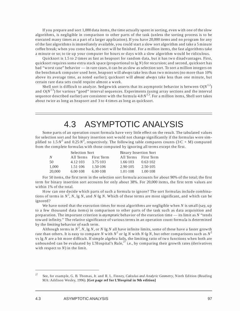
97
If you prepare and sort 1,000 data items, the time actually spent in sorting, even with one of the slowalgorithms, is negligible in comparison to other parts of the task (unless the sorting process is to beexecuted many times as a part of a larger application). If you have 20,000 items and no program for anyof the fast algorithms is immediately available, you could start a slow sort algorithm and take a 5 minutecoffee break; when you come back, the sort will be finished. For a million items, the fast algorithms takea minute or so; to tie up your computer for hours or days with a slow algorithm would be ridiculous.
Quicksort is 1.5 to 2 times as fast as heapsort for random data, but it has two disadvantages. First,quicksort requires some extra stack space (proportional to lg N) for recursion; and second, quicksort hasbad “worst case” behavior — in rare cases, it can be as slow as selection sort. To sort a million integers onthe benchmark computer used here, heapsort will always take less than two minutes (no more than 10%above its average time, as noted earlier); quicksort will almost always take less than one minute, butcertain rare data sets could require almost a week.
Shell sort is difficult to analyze. Sedgewick asserts that its asymptotic behavior is between O(N1.2)and O(N1.5) for various “good” interval sequences. Experiments (using array sections and the intervalsequence described earlier) are consistent with the formula 4.8·N1.3. For a million items, Shell sort takesabout twice as long as heapsort and 3 to 4 times as long as quicksort.
4.3 ASYMPTOTIC ANALYSISSome parts of an operation count formula have very little effect on the result. The tabulated values
for selection sort and for binary insertion sort would not change significantly if the formulas were sim-plified to 1.5·N2 and 0.25·N2, respectively. The following table compares counts (3·C + M) computedfrom the complete formulas with those computed by ignoring all terms except the first.
Selection Sort Binary Insertion SortN All Terms First Term All Terms First Term50 4.12·103 3.75·103 1.66·103 0.63·1021,000 1.51·106 1.50·106 2.90·105 2.50·10520,000 6.00·108 6.00·108 1.01·108 1.00·108
For 50 items, the first term in the selection sort formula accounts for about 90% of the total; the firstterm for binary insertion sort accounts for only about 38%. For 20,000 items, the first term values arewithin 1% of the total.
How can one decide which parts of such a formula to ignore? The sort formulas include combina-tions of terms in N2, N, lg N, and N·lg N. Which of these terms are most significant, and which can beignored?
We have noted that the execution times for most algorithms are negligible when N is small (say, upto a few thousand data items) in comparison to other parts of the task such as data acquisition andpreparation. The important criterion is asymptotic behavior of the execution time — its limit as N “tendstoward infinity.” The relative significance of various terms in an operation count formula is determinedby the limiting behavior of each term.
Although terms in N2, N, lg N, or N·lg N all have infinite limits, some of these have a faster growthrate than others. It is easy to compare N with N2 or lg N with N·lg N, but other comparisons such as N2
vs lg N are a bit more difficult. If simple algebra fails, the limiting ratio of two functions when both areunbounded can be evaluated by L’Hospital’s Rule,27 i.e., by comparing their growth rates (derivativeswith respect to N) in the limit.
27 See, for example, G. B. Thomas, Jr. and R. L. Finney, Calculus and Analytic Geometry, Ninth Edition (ReadingMA: Addison Wesley, 1996). [Get page ref for L’Hospital in 9th edition]
4.3 ASYMPTOTIC ANALYSIS
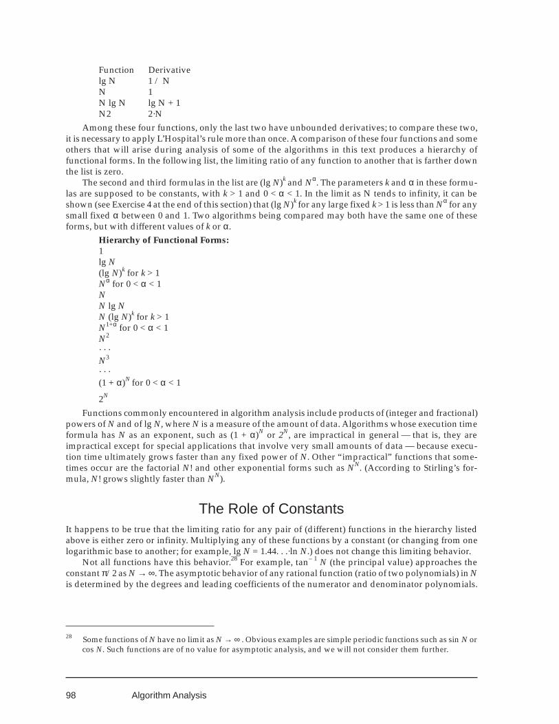
98
Function Derivativelg N 1 / NN 1N lg N lg N + 1N2 2·N
Among these four functions, only the last two have unbounded derivatives; to compare these two,it is necessary to apply L’Hospital’s rule more than once. A comparison of these four functions and someothers that will arise during analysis of some of the algorithms in this text produces a hierarchy offunctional forms. In the following list, the limiting ratio of any function to another that is farther downthe list is zero.
The second and third formulas in the list are (lg N)k and Nα. The parameters k and α in these formu-las are supposed to be constants, with k > 1 and 0 < α < 1. In the limit as N tends to infinity, it can beshown (see Exercise 4 at the end of this section) that (lg N)k for any large fixed k > 1 is less than Nα for anysmall fixed α between 0 and 1. Two algorithms being compared may both have the same one of theseforms, but with different values of k or α.
Hierarchy of Functional Forms:1lg N(lg N)k for k > 1Nα for 0 < α < 1NN lg NN (lg N)k for k > 1N1+α for 0 < α < 1N2
· · ·N3
· · ·(1 + α)N for 0 < α < 1
2N
Functions commonly encountered in algorithm analysis include products of (integer and fractional)powers of N and of lg N, where N is a measure of the amount of data. Algorithms whose execution timeformula has N as an exponent, such as (1 + α)N or 2N, are impractical in general — that is, they areimpractical except for special applications that involve very small amounts of data — because execu-tion time ultimately grows faster than any fixed power of N. Other “impractical” functions that some-times occur are the factorial N! and other exponential forms such as NN. (According to Stirling’s for-mula, N! grows slightly faster than NN).
The Role of ConstantsIt happens to be true that the limiting ratio for any pair of (different) functions in the hierarchy listedabove is either zero or infinity. Multiplying any of these functions by a constant (or changing from onelogarithmic base to another; for example, lg N = 1.44. . .·ln N.) does not change this limiting behavior.
Not all functions have this behavior.28 For example, tan– 1 N (the principal value) approaches theconstant π/2 as N → ∞. The asymptotic behavior of any rational function (ratio of two polynomials) in Nis determined by the degrees and leading coefficients of the numerator and denominator polynomials.
28 Some functions of N have no limit as N → ∞ . Obvious examples are simple periodic functions such as sin N orcos N. Such functions are of no value for asymptotic analysis, and we will not consider them further.
Algorithm Analysis
99
Consider the two rational functions (a N5 + ...) / (N2 + ...) and (b N5 + ...) / (N2 + ...) where the omittedparts are polynomials of lower degree that may be different for the two functions. The functions haveasymptotic behavior a N3 and b N3 respectively; the limiting ratio of the two rational functions is a / b.
The Complexity of an Algorithm: Big OhAsymptotic analysis employs a notation that reduces a formula to its most significant terms, ignoringterms that are insignificant in the limit. The asymptotic order of a function is found as follows:
Express the function as a sum of terms.In principle, it is necessary to compare each term with all of the others. If the limiting ratio of any
two terms F and G is zero, F may be deleted from the sum.All of the terms that remain have the same asymptotic behavior. Any such term, with constant
factors deleted, may be said to be the asymptotic behavior of the function.Consider the formula f(N) = N2 (3 +4 tan– 1 N) +lg N. Expressed as a sum of terms, this formula
becomes 3N2 +4·N2 tan–1 N + lg N. The logarithm is not significant in the limit, so it is deleted and twoterms remain. The asymptotic behavior of f(N) can be said to be either N2 or N2 tan– 1 N — the simplerform would ordinarily be preferred.
We say that f(N) is O(N2) or is O(N2 tan– 1 N); again, the simpler form is preferred. Orally, one wouldsay that f(N) is “big oh” N2 or that it has “big oh” N2 asymptotic behavior. This means that some constantmultiple of N2 is an upper bound for f(N) as N grows large. If f(N) is an estimate for the running time ofsome algorithm, it can be said that the “complexity” of the algorithm is N2.
It is not always easy to find such an upper bound for the running time of an algorithm, in terms ofthe amount of data. If such bounds can be obtained for different algorithms that might be applied to thesame application, they can be used to compare the algorithms with regard to asymptotic running time orcomplexity.
Asymptotic upper bounds do not give the whole story, of course. Average behavior estimates canalso be valuable; lower bounds are sometimes useful as well. The quicksort operation count formula3.75·N lg N + 13.5·N – 13.5 is an estimate of average behavior. The worst case for this algorithm (if eachpivot happens to be the largest or smallest data item) is O(N2), but careful implementation of the algo-rithm can ensure that this case occurs rarely. The best case (lower bound) for straight insertion sorting(but not for binary insertion) is proportional to N, which is achieved when the data is already in order,because the inner loop always exits after the first comparison in that case.
When two algorithms have the same complexity, it may be desirable to compare them further, tak-ing into account constants that appear in the bounds or estimates, and perhaps other considerations aswell:• The formula 1.5·N2 + 0.7·N lg N + 3.5·N – 0.7·lg N – 3 for selection sorting is an upper bound, but it
differs only slightly from the estimated average and from the lower bound. The binary insertionformula 0.25·N2 + 4.5·N lg N – 4.8·N – 2.9 is again an estimated average; the worst case for thisalgorithm is 0.5·N2 +4.5·N lg N – 4.8·N – 2.9 and its best case is 4.5·N·lg N – 4.3·N – 2.9. For sorting alarge amount of data that is almost in order, the term in N lg N makes binary insertion inferior tostraight insertion.
• For random data, both Quicksort and Heapsort have complexity O(N lg N), but the constant factorin the leading term for Heapsort is about twice that of Quicksort. However, the complexity ofQuicksort in the worst case is O(N2) while the worst case for Heapsort remains O(N lg N).
4.3 ASYMPTOTIC ANALYSIS
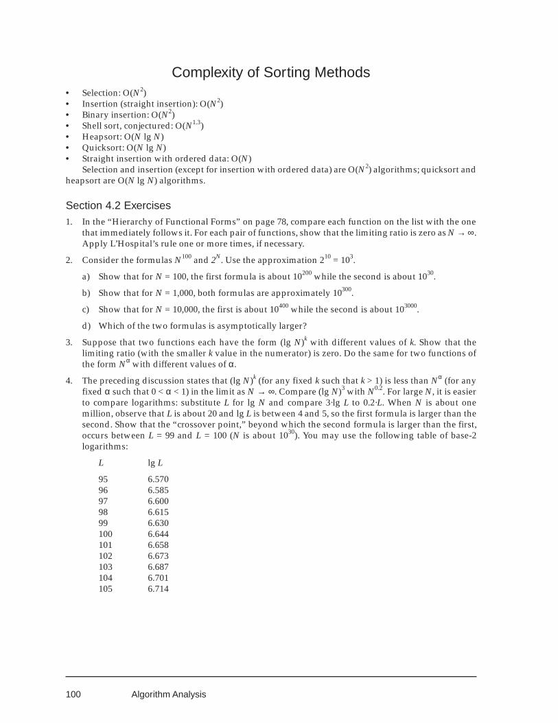
100
Complexity of Sorting Methods• Selection: O(N2)• Insertion (straight insertion): O(N2)• Binary insertion: O(N2)• Shell sort, conjectured: O(N1.3)• Heapsort: O(N lg N)• Quicksort: O(N lg N)• Straight insertion with ordered data: O(N)
Selection and insertion (except for insertion with ordered data) are O(N2) algorithms; quicksort andheapsort are O(N lg N) algorithms.
Section 4.2 Exercises1. In the “Hierarchy of Functional Forms” on page 78, compare each function on the list with the one
that immediately follows it. For each pair of functions, show that the limiting ratio is zero as N → ∞.Apply L’Hospital’s rule one or more times, if necessary.
2. Consider the formulas N100 and 2N. Use the approximation 210 = 103.
a) Show that for N = 100, the first formula is about 10200 while the second is about 1030.
b) Show that for N = 1,000, both formulas are approximately 10300.
c) Show that for N = 10,000, the first is about 10400 while the second is about 103000.
d) Which of the two formulas is asymptotically larger?
3. Suppose that two functions each have the form (lg N)k with different values of k. Show that thelimiting ratio (with the smaller k value in the numerator) is zero. Do the same for two functions ofthe form Nα with different values of α.
4. The preceding discussion states that (lg N)k (for any fixed k such that k > 1) is less than Nα (for anyfixed α such that 0 < α < 1) in the limit as N → ∞. Compare (lg N)3 with N0.2. For large N, it is easierto compare logarithms: substitute L for lg N and compare 3·lg L to 0.2·L. When N is about onemillion, observe that L is about 20 and lg L is between 4 and 5, so the first formula is larger than thesecond. Show that the “crossover point,” beyond which the second formula is larger than the first,occurs between L = 99 and L = 100 (N is about 1030). You may use the following table of base-2logarithms:
L lg L
95 6.57096 6.58597 6.60098 6.61599 6.630100 6.644101 6.658102 6.673103 6.687104 6.701105 6.714
Algorithm Analysis
101
4.4 MATHEMATICAL INDUCTIONAccording to Section 3.3, the forumula tn = b·n lg n + a·(n – 1) satisfies the recurrence relation t1 = 0, tn =a + b·n + 2·tn/2 when n is a power of 2. The present section shows how to use the method of mathematicalinduction to verify this formula, and how to apply the method to other similar problems.
The method depends upon the Induction Principle, which states that a function of an integer argu-ment is valid for all nonnegative values of its argument, provided that both of the following can beshown:1. The function is valid for the argument value 0; and
2. Validity of the function for any nonnegative argument value m implies validity for m + 1.In this particular application, the substitution n = 2k+1 gives a new independent variable k that takes
on nonnegative integer values. With sk+1 = tn; sk = tn/2, it is to be shown that the function sk = b·k·2k + a·(2k–1) satisfies the recurrence relation sk+1 = a + b·2k+1 + 2·sk with s0 = 0.
Step one of the method requires that the proposed function be verified for k = 0:s0 = b·0·20 + a(20 – 1) = 0Step two assumes that the proposed function is correct for an arbitrary (nonnegative) value k = m:s(m) = b·m·2m + a·2m – a
and then uses this assumption to compute the function value for k = m + 1 from the given recurrencerelation:
sm+1 = a + b·2m+1 +2·(b·m·2m + a·2m – a) = b·(m + 1)·2m+1 + a·2m+1 – aThis calculation shows that the assumption for k = m implies that the proposed function is correct for
the next value k = m + 1.Thus both requirements of the Induction Principle are satisfied and the proposed function is correct
for all nonnegative values of k. The original formula in n is therefore valid whenever n is a power of 2with a positive integer exponent.
Section 4.4 Exercises1. Fibonacci numbers: Use mathematical induction to prove that the recurrence F0 = 0, F1 = 1, Fm+2 =
Fm+1 + Fm is satisfied by the formula FN = (αN – βN)/(α – β). First, show that the formula gives thecorrect result when N is zero or 1. Then, assuming that the formula is correct for N = m and for N =m + 1, write out Fm+1 + Fm. Show algebraically that this sum is equal to (αm+2 – βm+2)/(α – β), using thefact that α and β are roots of the equation x2 – x – 1 = 0.
2. Shell sort interval sequence: Use mathematical induction to prove that the recurrence h0 = 1, hk+1 =3·hk + 1 is satisfied by the formula hk = (3·k – 1) / 2.
4.4 MATHEMATICAL INDUCTION
102
Chapter 5 Linked Lists
Although arrays can be accessed very rapidly and efficiently, they have one major shortcoming: Anarray has a fixed size that cannot be changed after data has been stored in it. On the other hand, a linkedlist is stored dynamically and becomes larger or smaller when data is added or removed. Data can beinserted or deleted at the beginning or end of a linked list or at a specific position in the middle.
A linked list is a sequence of nodes connected with pointers. Each node is a structure, and one of itscomponents is a pointer to the remainder of the list. For example:
type :: Node_Typetype (Info_Type) :: Infotype (Node_Type), pointer :: Next_NP
end type Node_Type
The pointer in the last node of a linked list is null because the remainder of the list is empty.A linked list is accessed through a root pointer whose target is the first node — unless the list is
empty, in which case the root pointer is null. The root is declared as a variable with the pointer attribute,of the data type that has been defined for the node structures.
type (Node_Type), pointer :: Root_NP => null( )The root is declared as a pointer variable in a main program, a subprogram, or a module. The rootpointer itself is usually not a dynamically allocated object, but its target node is allocated in dynamicstorage during program execution, by the following statement:
allocate( Root_NP )Each additional node in the list is allocated dynamically as required, as the target of the pointer compo-nent in a previously allocated node.
5.1 LINKED LIST NODE OPERATIONS
Let the nodes of a linked list be structures of type Node_Type , with a data component named Info anda pointer component named Next_NP:
type :: Node_Typetype (Info_Type) :: Infotype (Node_Type), pointer :: Next_NP => null( )
end type Node_Type
The declared (target) type of the pointer component is Node_Type ; this pointer provides access to theremainder of the linked list beyond the node in which it appears. Nodes are initialized with a nullpointer component; thus a new node has no target until steps are taken to incorporate it into the linkedlist.
103
Node_Type
Info_Type
Next_NP
Key
Count(2)Count(1)
Info
The data component, Info, occupies a structure of type Info_Type ; for simplicity, let this structureconsist of a character string component named Key and an integer vector component named Data. Thetype definition for Info_Type specifies default initialization for the character and integer components.
type :: Info_Typecharacter (len = S_LEN) :: Key = " "integer :: Data(2) = 0
end type Info_Type
FIGURE 5.1. Derived types for linked list nodes
The forward pointer in each node and the root pointer may be viewed as pointers to the remainderof the list, not merely to the next node. Unless the remainder of the list is empty, it is a node that containsan information component and a pointer to the (further) remainder.29
Create ListA linked list is created by a type declaration for the root pointer. Initially, there are no nodes in the list;the root pointer has no target (see Fig. 5.2a). The derived type definition specifies initial nullification forthe root pointer.30
type (Node_Type), pointer :: Root_NP => null( )
5.1 LINKED LIST NODE OPERATIONS
29 This point of view is explored further by Brainerd, et al in Programmer’s Guide to F (Albuquerque: Unicomp,1996), 280
30 Default initiallization of structure components as shown here, including initial nullification of pointers, ispossible with Fortran 95. Fortran 90 requires assignment statements to initialize data components and nul-lify( ) statements for pointers. Electronically distributed examples include alternative Fortran 90 versions.
104
a) Create List
b) Insert Target Node
?
?
c) Delete Target Node
?
?
FIGURE 5.2. Operations to Create, Insert, and Delete a linked list node
Insert Target NodeA simple operation on a linked list is the insertion of a new node as the target of a given pointer (see Fig.5.2b). For example, a node may be added to an empty list by inserting it as the target of Root_NP; or anode may be added as the target of the forward pointer in an existing node. An information structure tobe assigned as the Info component of the new node may be passed as an argument to an insertion proce-dure. The operation Insert_Target( Arg_NP, Item ) has two parts:1. Allocate a new node as the target of a temporary pointer, Temp_NP. Give values to all components of
the new node. Copy Arg_NP (by pointer assignment) to the forward component of the new node,Temp_NP % Next_NP , thus linking the remainder of the list to the newly allocated node.
Arg_NP must be copied before it is changed; otherwise, changing Arg_NP would remove the onlypointer to the remainder (if any) of the linked list, and the remainder of the list would be lost.
2. Copy Temp_NP (by pointer assignment) to Arg_NP, thus linking the remainder of the list (includingthe new node) to Arg_NP .
subroutine Insert_Target( Arg_NP, Item )type (Node_Type), pointer :: Arg_NP, Temp_NPtype (Info_Type), intent(in) :: Item
! start subroutine Insert_Targetallocate( Temp_NP )Temp_NP % Info = ItemTemp_NP % Next_NP => Arg_NPArg_NP => Temp_NPreturn
end subroutine Insert_Target
As shown below, a linked list can be generated by calling this procedure repeatedly with the rootpointer Root_NP as the argument. Each call will allocate a new node and insert it as the target of Root_NP.Thus, after each call the new node will be the first node in the linked list and the sequence of nodes thatpreviously comprised the linked list will follow the new node.
Linked Lists
105
Delete Target NodeThe procedure Delete_Node( Arg_NP ) deletes the linked list node that is the target of Arg_NP, asillustrated in Fig. 5.2c. The successor of the deleted node becomes the target of Arg_NP (unless thedeleted node was the last node in the linked list, in which case the null successor pointer is copied toArg_NP). Here, the procedure is implemented as a function whose result value is a copy of the Infocomponent of the deleted node. The procedure consists of the following steps:1. Copy Arg_NP (by pointer assignment) to Temp_NP. This must be done before Arg_NP is changed (at
step 3); otherwise, there would be no way to delete the node that is the target Arg_NP . If Arg_NP hasa target, continue with the remaining steps; otherwise, skip them. (In the latter case, the functionresult variable retains its default initialization value).
2. Assign the Info component, in the node that will be deleted, to the function result variable.
3. Change Arg_NP so that its target is the successor (if any) of the node to be deleted — that is, theNext_NP component of the node to be deleted is copied (by pointer assignment) to Arg_NP . If thedeleted node has no successor, its Next_NP component is a null pointer and copying it has the effectof nullifying Arg_NP .
4. Deallocate Temp_NP, which is now the only pointer whose target is the node to be deleted; thus,deallocating Temp_NP deletes the node. This deallocation must take place after Next_NP has beencopied to Arg_NP (at step 3).
function Delete_Target( Arg_NP ) result( Item )type (Node_Type), pointer :: Arg_NP, Temptype (Info_Type) :: Item
! start function Delete_TargetTemp => Arg_NPItem = Arg_NP % InfoArg_NP => Arg_NP % Next_NPdeallocate( Temp )return
end function Delete_Target
Print Target NodeThe procedure Print_Target( Arg_NP ) prints components of the target of Arg_NP. Fortran does notpermit pointers in input or output lists; only the nonpointer component Arg_NP % Info is printed.
subroutine Print_Target( Arg_NP )type (Node_Type), pointer :: Arg_NP
! start subroutine Print_Targetprint *, " Print: ", Arg_NP % Inforeturn
end subroutine Print_Target
5.1 LINKED LIST NODE OPERATIONS
106
Modify Target NodeThe procedure Modify_Target( Arg_NP ) performs a predetermined modification upon the nodethat is the target of Arg_NP. In our examples, we increment Arg_NP % Info % Data(2) . This elementthus contains a count of the number of occurrences of the corresponding key, if it was given the value 1when the node was inserted.
subroutine Modify_Target( Arg_NP )type (Node_Type), pointer :: Arg_NP
! start subroutine Modify_TargetArg_NP % Info % Data(2) = Arg_NP % Info % Data(2) + 1return
end subroutine Modify_Target
5.2 OPERATIONS ON WHOLE LINKEDLISTS
Making a Linked List by Insertion at the RootThe subroutine Insert_Target can be called repeatedly with Root_NP as its argument. A loop such asthe following will read data and insert it at the root until the end of input is detected.
type (Node_Type), pointer:: Root_NP:
doread (1, *, iostat = EoF) Temp_NP % Keyif (EoF < 0) exitTemp_NP % Data(1) = LoopTemp_NP % Data(2) = 1call Insert_Target( Root_NP, Temp_NP )
end do
The read statement accepts data for a node of the linked list and inserts the node as the target ofRoot_NP. The data that was read first will be at the end of the linked list, and the data that was read mostrecently will be in the node that is the final target of Root_NP.
Print ListVery common in linked list applications is the use of a declared “traveling node pointer,” here calledTrav_NP, that points to the current node and then advances to the next node.
The first execution step copies Root_NP to Trav_NP. Just before the end of each iteration, the forwardpointer component of the current node, Trav_NP % Next_NP , is copied to Trav_NP. When the end of thelist is reached, Trav_NP is null. The subroutine Print_List prints data from the current node and thenadvances to the next node to print the remainder of the list. The entire list will be printed in order,beginning with the root and proceeding to the tail.
Linked Lists
107
type (Node_Type), pointer:: Root_NP:
subroutine Print_List( )type (Node_Type), pointer :: Trav_NP
! start subroutine Print_ListTrav_NP => Root_NPdo while (associated( Trav_NP ))
call Print_Target( Trav_NP )Trav_NP => Trav_NP % Next_NP ! Advance to next node
end doreturn
end subroutine Print_List
Delete ListA traveling pointer is not needed for repeatedly deleting the first node (the target of the root pointer)until the list is empty:
type (Node_Type), pointer:: Root_NP:
do while (associated( Root_NP ))print *, " Deleted: ", Delete_Target( Root_NP )
end do
Searching in a Linked ListA linked list search can easily be implemented with a traveling pointer. The following example showshow to perform a linear search in a list, beginning at Root_NP, for a node wherein Info % Key matchesthe Key component of the input Item. When a match is found, a message is printed and data in the targetnode is modified. If the end of the list is reached, the message " Not Found." is printed.
type (Node_Type), pointer:: Root_NP:
subroutine Search_List( Item )type (Info_Type), intent(in) :: Itemtype (Node_Type), pointer:: Trav_NP
! start subroutine Search_ListTrav_NP => Root_NPdo
if (associated( Trav_NP )) thenif (Item % Key == Trav_NP % Info % Key) then
print *, Item % Key, " Found."call Modify_Target( Trav_NP, Item % Data(1) )return
end ifelse
print *, Item % Key, " Not Found."return
end ifTrav_NP => Trav_NP % Next_NP ! Keep searching.
end doend subroutine Search_List
5.2 OPERATIONS ON WHOLE LINKED LISTS
108
The situation is not quite so simple, however, if the linkage is to be modified when a particular key isfound in the middle of a linked list. Procedures such as Insert_Target and Delete_Target (de-scribed earlier) link remaining nodes of the list only to Trav_NP which is a copy of the an actual list link;they do not correctly modify the linkage of the actual list. This situation is discussed in more detail in thefollowing paragraphs.
Maintaining a Large Ordered ListSuppose that a linked list is ordered according to a key, and a new item is to be inserted. A linear searchfor the new key, beginning at the root of the linked list, has three possible outcomes.1. An item in the linked list with a matching key may be found. In this case no new item is to be
inserted. In our examples, the matching item is modified. When the search terminates, the target ofTrav_NP is the node with a matching key.
2. If all items in the list have keys smaller than the new one, the end of the linked list will be reached. Inthis case, Trav_NP is null when the search terminates. The new item is to be inserted at the end, asthe new successor of the previous target of Trav_NP .
3. Otherwise, the search terminates when an item with a larger key is found. The node with the largerkey is the target of Trav_NP , and the new item is to be inserted as the new successor of the previoustarget of Trav_NP .There is a difficulty in either case 2 or case 3, because Trav_NP has already moved beyond the inser-
tion point when the search terminates and a larger key or a null pointer has been encountered. It wouldbe easy to insert a new item as the successor of the Trav_NP target node: it is only necessary to callInsert_Target with Trav_NP % Next_NP as the argument. But the forward node pointer in thepreceding node is no longer accessible.
A similar problem arises when an item that matches a given key is to be deleted from a linked list.With the linked list search procedure described earlier, Trav_NP has again moved beyond the deletionpoint when the search terminates, and the pointer whose target is to be deleted from the linked list is nolonger accessible.
The heart of the difficulty lies in the fact that Trav_NP is a copy of the pointer Next_NP in the prede-cessor node; therefore, deleting the target of Trav_NP or creating a new target for Trav_NP does notchange the actual linkage of the linked list.
The obvious solution to this difficulty, described by many authors, is very inelegant and wasteful: Atravelling pointer points to the predecessor of the node that is currently being examined. This requiresextra steps at the beginning of a search (or other traversal of the linked list). One method declares theroot as a separate pointer; this requires that a different sequence of statements be executed to examinethe root target node. An alternative method creates the list with an otherwise unused “header node” asthe target of the root pointer.
Two strategies that avoid these complications are discussed in Sections 5.3 and 5.4:1. The search may be performed recursively, with the forward node pointer as the argument at each
recursive call; or
2. The forward node pointer — or, in Fortran, a BOX containing the forward node pointer — may beassigned as the target of the traveling pointer. With a BOX that performs the role of the predecessornode, the Fortran syntax is still somewhat complicated. However, this method does not require aseparate statement sequence nor a separate header node with wasted space for nonpointer nodecomponents (which, in some applications, can be significant).
Linked Lists
109
5.3 PROCESSING LINKED LISTSRECURSIVELY
The actual argument to a recursive linked list procedure is a pointer to the remainder of a list (initiallyRoot_NP, the pointer to the entire list). The procedure processes the current node and then calls itselfrecursively to process the remainder (unless the remainder is empty). While processing the current node,the procedure may modify the dummy argument pointer. Such modifications affect the actual linkage ofthe list, and not merely a copy of the argument pointer.
The following example shows how to insert a new item into an ordered linked list. Arguments in theinitial call to the recursive subroutine are Root_NP and the data to be inserted.
The outer if construct tests whether the current node pointer is associated (i.e., whether it has anactual target).• If the current node pointer is not null, the inner if construct compares the Key in the current node,
referred to as Arg_NP % Info % Key , with the Key component of the given item. This comparisonhas three possible outcomes:
1. If the keys match, information in the current node is to be modified.
2. If Arg_NP % Info % Key is larger, no matching key will be found — the search has passed thepoint where a match would have occurred — so the given item is inserted ahead of the givennode. The procedure Insert_Target discussed earlier performs this operation and correctlymodifies the current input pointer.
3. Otherwise, Arg_NP % Info % Key is smaller than the search key, so the procedure is calledrecursively to search the remainder of the list.
• If the current node pointer is null, the else block of the outer if construct is executed and the givenitem is inserted at the end of the list.
recursive subroutine Look_Up( Arg_NP, Item )type (Node_Type), pointer :: Arg_NPtype (Info_Type), intent(in) :: Item
! start subroutine Look_Upif (associated( Arg_NP )) then
if (Item % Key == Arg_NP % Info % Key) thencall Modify_Target( Arg_NP, Item )
else if (Arg_NP % Info % Key > Item % Key) thencall Insert_Target( Arg_NP, Item ) ! Insert before next node.
elsecall Look_Up( Arg_NP % Next_NP ) ! Keep looking.
end ifelse
call Insert_Target( Arg_NP, Item ) ! Insert at end of linked list.end ifreturn
end subroutine Look_Up
This recursive approach is very elegant, but the time and space overhead imposed by recursionleave some scholars unconvinced of its merits. A new activation record (see Section 3.1) is created ateach recursive call — that is, for each node encountered by the linked list operation. For a very longlinked list, the amount of extra storage occupied by these activation records may be intolerable. On theother hand, a long list will itself necessarily occupy a great deal of storage unless the amount of data ineach node is trivial.
5.2 OPERATIONS ON WHOLE LINKED LISTS
110
Nevertheless, for long lists it is well to minimize the space occupied by each activation record. Inparticular, the procedure Look_Up has an argument Item that might be a large data structure in anactual application; it would be well to avoid storing redundant copies of this Item. A solution is to con-struct the subroutine Look_Up as a nonrecursive “wrapper.” The application program calls Look_Up ,which in turn calls a recursive internal procedure R_Look_Up that inherits Item from the wrapper. Theargument Item is stored only in the activation record for the wrapper; the activation record for R_Look_Upis now quite small because there are no local variables and the only argument is a pointer.
Say It with Fortran
Example 14
! Example 14. Linked List with Recursionmodule D14_M
implicit nonepublic :: Look_Up, Print_List, Delete_Listinteger, parameter, public :: S_LEN = 20type, public :: Info_Type
character (len = S_LEN) :: Keyinteger, dimension(2) :: Data = (/ 0, 1 /)
end type Info_Typetype, private :: Node_Type
type (Info_Type) :: Infotype (Node_Type), pointer :: Next_NP => Null( )
end type Node_Typetype (Node_Type), pointer, private :: Root_NP => Null( )
contains
subroutine Look_Up( Item )type (Info_Type), intent(in out) :: Item
! start subroutine Look_Upcall R_Look_Up( Root_NP )return
contains
recursive subroutine R_Look_Up( Arg_NP )type (Node_Type), pointer :: Arg_NP
! start subroutine R_Look_Upif (associated ( Arg_NP )) then
if (Item % Key == Arg_NP % Info % Key) thencall Modify_Target( Arg_NP, Item )
else if (Arg_NP % Info % Key > Item % Key) thencall Insert_Target( Arg_NP, Item ) ! Insert ahead of next node.
elsecall R_Look_Up( Arg_NP % Next_NP ) ! Keep looking.
end ifelse
call Insert_Target( Arg_NP, Item ) ! Insert at end of linked list.end ifreturn
end subroutine R_Look_Up
Linked Lists
111
subroutine Modify_Target( Arg_NP )type (Node_Type), pointer :: Arg_NP
! start subroutine Modify_TargetArg_NP % Info % Data(2) = Arg_NP % Info % Data(2) + 1return
end subroutine Modify_Target
subroutine Insert_Target( Arg_NP, Item )type (Node_Type), pointer :: Arg_NP, Temp_NPtype (Info_Type), intent(in) :: Item
! start subroutine Insert_Targetallocate( Temp_NP )Temp_NP % Info = ItemTemp_NP % Next_NP => Arg_NPArg_NP => Temp_NPreturn
end subroutine Insert_Target
end subroutine Look_Up
subroutine Print_List( )! start subroutine Print_List
call R_Print_List( Root_NP )return
contains
subroutine R_Print_List( Arg_NP )type (Node_Type), pointer :: Arg_NP
! start subroutine R_Print_Listif (associated ( Trav_NP )) then
call Print_Target( Trav_NP )call R_Print_List( Arg_NP % Next_NP ) ! Advance to next node
end ifreturn
end subroutine R_Print_List
subroutine Print_Target( Arg_NP )type (Node_Type), pointer :: Arg_NP
! start subroutine Print_Targetprint *, " Print: ", Arg_NP % Inforeturn
end subroutine Print_Target
end subroutine Print_List
subroutine Delete_List( )! start subroutine Delete_List
call R_Delete_List( Root_NP )return
contains
5.3 PROCESSING LINKED LISTS RECURSIVELY
112
subroutine R_Delete_List( )! start subroutine R_Delete_List
if (associated ( Root_NP )) thenprint *, " Deleted: ", Delete_Target( Root_NP )
Delete at root: Next call deletes at the same point.
call R_Delete_List( )end ifreturnend subroutine R_Delete_List
function Delete_Target( Arg_NP ) result(Item)type (Node_Type), pointer :: Arg_NP, Temptype (Info_Type) :: Item
! start function Delete_TargetTemp_NP => Arg_NPItem = Arg_NP % InfoArg_NP => Arg_NP % BOX % Next_NPdeallocate( Temp_NP )
end function Delete_Target
end subroutine Delete_List
end module D14_M
program D14use D14_Mimplicit noneinteger :: EoFtype (Info_Type) :: Item
! start program D14open (1, file = "dxf.txt", status = "old", action = "read", &
position = "rewind")do
read (1, *, iostat = EoF) Temp_NP % Keyif (EoF < 0) exitItem % Data(1) = Item % Data(1) + 1call Look_Up( Item )
end docall Print_List( )call Delete_List( )stop
end program D14
As mentioned earlier, a linked list may be viewed as a recursive data structure: Each node containsdata as well as a pointer to the remainder of the list. Besides its philosophical elegance, recursive linkedlist processing fortuitously circumvents a syntactic shortcoming of Fortran and of some other program-ming languages. The recursive technique passes the pointer argument (at each recursive call) by refer-ence: what is actually transmitted is a pointer to the argument pointer. Pointers to pointers are needed,and recursion provides this facility in a (syntactically) simple manner. This philosophical elegance andsyntactic simplicity are achieved at the expense of extra space and time overhead imposed by the mecha-nism of recursion, although with some care the space overhead can be minimized. Converting the tailrecursion in this program to iteration without introducing significant syntactic complication seems im-possible.
Linked Lists
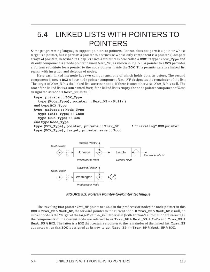
113
Johnson
Predecessor Node
Remainder of ListLincoln
Current Node
Traveling PointerRoot Pointer
Washington
Predecessor Node
Traveling PointerRoot Pointer
5.4 LINKED LISTS WITH POINTERS TOPOINTERS
Some programming languages support pointers to pointers. Fortran does not permit a pointer whosetarget is a pointer, but it permits a pointer to a structure whose only component is a pointer. (Comparearrays of pointers, described in Chap. 2). Such a structure is here called a BOX: its type is BOX_Type andits only component is a node pointer named Next_NP, as shown in Fig. 5.3. A pointer to a BOX providesa Fortran substitute for a pointer to the node pointer inside the BOX. This permits iterative linked listsearch with insertion and deletion of nodes.
Here each linked list node has two components, one of which holds data, as before. The secondcomponent is now a BOX whose node pointer component Next_NP designates the remainder of the list:The target of Next_NP is the linked list successor node, if there is one; otherwise, Next_NP is null. Theroot of the linked list is a BOX named Root; if the linked list is empty, the node pointer component of Root,designated as Root % Next_NP , is null.
type, private :: BOX_Typetype (Node_Type), pointer :: Next_NP => Null( )
end type BOX_Typetype, private :: Node_Type
type (Info_Type) :: Infotype (BOX_Type) :: BOX
end type Node_Typetype (BOX_Type), pointer, private :: Trav_BP ! "traveling" BOX pointertype (BOX_Type), target, private, save :: Root
FIGURE 5.3. Fortran Pointer-to-Pointer technique
The traveling BOX pointer Trav_BP points to a BOX in the predecessor node; the node pointer in thisBOX is Trav_BP % Next_NP , the forward pointer to the current node. If Trav_BP % Next_NP is null, nocurrent node is the “target of the target” of Trav_BP. Otherwise (with Fortran’s automatic dereferencing),the components of the current node are referred to as Trav_BP % Next_NP % Info and Trav_BP %Next_NP % BOX. The latter is a BOX that contains a pointer to the remainder of the linked list; Trav_BPadvances when this BOX is assigned as its new target: Trav_BP => Trav_BP % Next_NP % BOX.
5.4 LINKED LISTS WITH POINTERS TO POINTERS
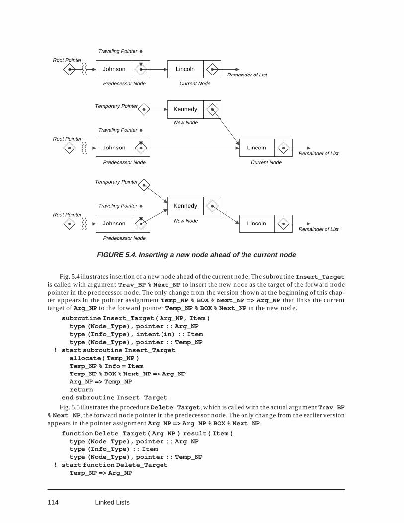
114
Fig. 5.4 illustrates insertion of a new node ahead of the current node. The subroutine Insert_Targetis called with argument Trav_BP % Next_NP to insert the new node as the target of the forward nodepointer in the predecessor node. The only change from the version shown at the beginning of this chap-ter appears in the pointer assignment Temp_NP % BOX % Next_NP => Arg_NP that links the currenttarget of Arg_NP to the forward pointer Temp_NP % BOX % Next_NP in the new node.
subroutine Insert_Target( Arg_NP, Item )type (Node_Type), pointer :: Arg_NPtype (Info_Type), intent(in) :: Itemtype (Node_Type), pointer :: Temp_NP
! start subroutine Insert_Targetallocate( Temp_NP )Temp_NP % Info = ItemTemp_NP % BOX % Next_NP => Arg_NPArg_NP => Temp_NPreturn
end subroutine Insert_Target
Fig. 5.5 illustrates the procedure Delete_Target , which is called with the actual argument Trav_BP% Next_NP , the forward node pointer in the predecessor node. The only change from the earlier versionappears in the pointer assignment Arg_NP => Arg_NP % BOX % Next_NP .
function Delete_Target( Arg_NP ) result( Item )type (Node_Type), pointer :: Arg_NPtype (Info_Type) :: Itemtype (Node_Type), pointer :: Temp_NP
! start function Delete_TargetTemp_NP => Arg_NP
Johnson
Remainder of List
Predecessor Node
Remainder of List
Remainder of List
Lincoln
Johnson
Kennedy
Johnson
Lincoln
Kennedy
Lincoln
Current Node
New Node
Current Node Predecessor Node
New Node
Predecessor Node
Traveling Pointer
Traveling Pointer
Traveling Pointer
Temporary Pointer
Temporary Pointer
Root Pointer
Root Pointer
Root Pointer
FIGURE 5.4. Inserting a new node ahead of the current node
Linked Lists
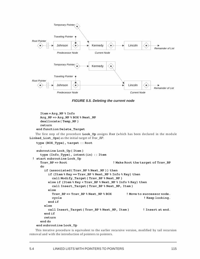
1155.4 LINKED LISTS WITH POINTERS TO POINTERS
Remainder of ListJohnson
Kennedy
Lincoln
Current Node Predecessor Node
Traveling Pointer
Temporary Pointer
Root Pointer
Remainder of ListJohnson Kennedy Lincoln
Current Node Predecessor Node
Traveling Pointer
Temporary Pointer
Root Pointer
FIGURE 5.5. Deleting the current node
Item = Arg_NP % InfoArg_NP => Arg_NP % BOX % Next_NPdeallocate( Temp_NP )return
end function Delete_Target
The first step of the procedure Look_Up assigns Root (which has been declared in the moduleLinked_List_Ops ) as the initial target of Trav_BP.
type (BOX_Type), target :: Root:
subroutine Look_Up( Item )type (Info_Type), intent(in) :: Item
! start subroutine Look_UpTrav_BP => Root ! Make Root the target of Trav_BPdo
if (associated( Trav_BP % Next_NP )) thenif (Item % Key == Trav_BP % Next_NP % Info % Key) then
call Modify_Target( Trav_BP % Next_NP )else if (Item % Key < Trav_BP % Next_NP % Info % Key) then
call Insert_Target( Trav_BP % Next_NP, Item )else
Trav_BP => Trav_BP % Next_NP % BOX ! Move to successor node.cycle ! Keep looking.
end ifelse
call Insert_Target( Trav_BP % Next_NP, Item ) ! Insert at end.end ifreturn
end doend subroutine Look_Up
This iterative procedure is equivalent to the earlier recursive version, modified by tail recursionremoval and with the introduction of pointers to pointers.
116
Say It with Fortran
Example 15. Shown here is a slightly modified version of the subroutine Look_Up for the Pointer toPointer technique, along with a main program. The BOX named Root is declared in module. Proceduresthat operate at the target level are the same as with recursion.
! Example 15. Linked list with pointers to pointers.module D15_M
implicit nonepublic :: Look_Up, Print_List, Delete_Listinteger, parameter :: S_LEN = 20type, public :: Info_Type
character (len = S_LEN) :: Keyinteger, dimension(2) :: Data = (/ 0, 1 /)
end type Info_Typetype, private :: BOX_Type
type (Node_Type), pointer :: Next_NP => Null( )end type BOX_Typetype, private :: Node_Type
type (Info_Type) :: Infotype (BOX_Type) :: BOX
end type Node_Typetype (BOX_Type), pointer, private :: Trav_BP !"traveling" BOX pointertype (BOX_Type), target, private, save :: Root
contains
subroutine Look_Up( Item )type (Info_Type), intent(in) :: Item
! start subroutine Look_UpTrav_BP => Root ! Make Root the target of Trav_BP
The if constructs have been rearranged to agree with the recursive Fortran program shown earlier. Note that theend do statement is never reached except from the cycle statement, which transfers control to the top of the doblock.
doif (associated ( Trav_BP % Next_NP )) then
if (Item % Key == Trav_BP % Next_NP % Info % Key) thencall Modify_Target( Trav_BP % Next_NP )
else if ( Item % Key < Trav_BP % Next_NP % Info % Key) thencall Insert_Target( Trav_BP % Next_NP, Item )
elseTrav_BP => Trav_BP % Next_NP % BOX ! Move to successor node.cycle ! Keep looking.
end ifelse
call Insert_Target( Trav_BP % Next_NP, Item ) ! Insert at end.end ifreturn
end docontains
subroutine Modify_Target( Arg_NP ):
end subroutine Modify_Target
Linked Lists
117
subroutine Insert_Target( Arg_NP, Item ):
end subroutine Insert_Target
end subroutine Look_Up
subroutine Print_List( )! start subroutine Print_List
Trav_BP => Rootdo while (associated ( Trav_BP % Next_NP ))
call Print_Target( Trav_BP )Trav_BP => Trav_BP % Next_NP % BOX ! Advance to next node
end doreturn
contains
subroutine Print_Target( Arg_BP ):
end subroutine Print_Target
end subroutine Print_List
subroutine Delete_List( )! start subroutine Delete_List
do while (associated ( Root % Next_NP ))print *, " Deleted: ", Delete_Target( Root )
end doreturn
contains
function Delete_Target( Arg_NP ) result(Item):
end function Delete_Target
end subroutine Delete_List
end module D15_M
Section 5.4 Exercises1. Write a recursive subroutine Print_List that prints information from the nodes of a linked list in
reverse order: If the argument pointer is not null, call Print_List with the forward pointer (i.e.,the remainder of the list) as its actual argument and then call Print_Target to print the current node.Calling Print_List with the root node as the actual argument will print the entire list in reverseorder.
2. Write a recursive subroutine Delete_List that deletes nodes from a linked list in reverse order: Ifthe argument pointer is not null, call Delete_List with the forward pointer (i.e., the remainder ofthe list) as its actual argument and then call Delete_Target to delete the current node. (Print theInfo component of each node as it is deleted.) Because the remainder of the list has already beendeleted, the current node is the last node at the time it is deleted, and its deletion nullifies the argu-ment pointer. Calling Delete_List with the root node as the actual argument will delete the entirelist in reverse order.
4. Implement the operation Look_Up with the data structure Item declared as a module variable;modify the module procedures to inherit Item and modify the main program to import it.
5.4 LINKED LISTS WITH POINTERS TO POINTERS
118
5.5. APPLICATIONS WITH SEVERALLINKED LISTS
The foregoing examples provide a single linked list whose root is declared in the list definition module.However, for many applications it is preferable to permit the consumer to create more than one list andto designate a specific list for each linked list operation. A root for each separate list is declared in theapplication program and can be passed to any of the linked list procedures. In the Pointer to Pointerversion shown here, each separate list is declared as a BOX, which becomes the initial target of Trav_BPin subroutine Look_Up .
type :: BOX_Typetype (Node_Type), pointer :: Next_NP => Null( )
end type BOX_Typetype :: Node_Type
type (Info_Type) :: Infotype (BOX_Type) :: BOX
end type Node_Type:
subroutine Look_Up( Arg_B, Item )type (BOX_Type), intent(in) :: Arg_Btype (Info_Type), intent(in) :: Item
! start subroutine Look_UpTrav_BP => Arg_B:
! Main program:
type (BOX_Type), target :: List1, List2, . . .:
call Look_Up( List1, Item ):
An array of linked lists may be required for some applications:! Main program
:type (BOX_Type), target, dimension(17) :: List
:call Look_Up( List(I), Item )
:
Multiply Linked ListsSome lists have more than one pointer in each node.
In a doubly-linked list, each node has both a forward pointer (to the successor node) and a backwardpointer (to the predecessor node). All of the node-level procedures are essentially unchanged except forthe extra overhead of modifying both pointer nodes during insertion or deletion. In a circular list, the lastnode points back to the first (i.e., in most implementations, to the successor of the root). These ways oforganizing the list are especially useful for certain applications, where it is necessary to access to thepredecessor of a given node or for data with a circular structure that has no natural beginning and end.
A threaded list consists of a single set of data that can be accessed according to any of several se-quences (threads). For example, it might be desirable to order a mailing list so that it could be printedsequentially by name or by postal ZIP code. Each node in a threaded list contains a pointer for each
Linked Lists
119
different key sequence that is to be applied; to facilitate insertions and deletions, each thread may belinked both forward and backward.
5.6 LINKED LISTS VS. ARRAYSA great many data processing applications store a collection of data items each of which contains a keyidentifying a unique item in the collection. For some applications the key is expanded to include asecondary key that distinguishes different items with the same primary key; in other cases a collectionwith unique keys merely serves as an index to the actual data — for example, a collection of pointers tosets of items that share a given key.
The two principal operations to be performed upon such a collection are:• Insert a new item into the collection if the key is not matched by that of any current item, or modify
the existing item (in some predetermined manner) if the key is matched.
• Search and delete an item with a given key.Each of these operations begins with a search to determine whether or not the the key is matched by
that of any item that is currently in the collection. For insertion, either outcome may be expected andappropriate actions are specified for either case. For deletion, however, an unmatched search key isconsidered an error.
Either an array or a linked list could be employed to hold such a collection. In either case, the dataitems may be stored either in key order or in some other manner unrelated to the key values. The follow-ing paragraphs discuss the advantages and disadvantages of these four possibilities. For the most part,it is assumed that the set of different keys in the collection at any given time is random and that keyspresented for insertion or deletion are random. However, some timing assumptions can have consider-able effect — for example, some applications insert almost all items into the collection before makingany deletions, so the current size of the collection at the time of a deletion is always nearly its maximumsize. In any case, it is assumed here that the modification phase of the insertion operation is straightfor-ward and does not require any significant further effort when the key is matched; also, the effort ofprocessing a deletion error is ignored. The most significant disadvantage of arrays, that the maximumsize of the collection must be known in advance, is not discussed at this point — it is assumed here thatsufficient array space is provided.
Array Implementation
Unordered Array
The search phase requires a linear search through the entire collection. If the search key is matched, theexpected number of comparisons is one-half the current size of the collection; if not, a comparison isrequired for every item currently in the collection.
If the search key is not matched, insertion is trivial: the new item is merely appended at the nexthigher subscript position beyond the current last item in the collection.
Deletion can occur at any point. Deleting an item requires that all items on its right be moved to theleft so that no gaps will remain between data items in the array. The expected number of items to bemoved as a result of the deletion is one-half the current size of the collection.
Ordered Array
Search in an ordered array can employ the binary search algorithm. Whether or not the search key ismatched, the expected number of comparisons is lg N where N is the current size of the collection.
5.5 LINKED LISTS VS. ARRAYS
120
If there is no match, the search locates the point at which the new item must be inserted. All items tothe right of the insertion point must be moved farther to the right (to a higher subscript position in thearray) to make room for the new item. The expected number of items to be moved is one-half the currentsize of the collection.
After the search phase, deletion is the same as for an unordered array: All items to the right of thedeletion point, estimated as one-half the current size of the collection, must be moved.
Linked List Implementation
Unordered Linked List
As in the array implementation, the search phase requires a linear search through the entire collection. Ifthe item is present, the expected number of comparisons is one-half the current size of the collection;otherwise, a comparison is required for every item currently in the collection.
If the search key is not matched, insertion is trivial: the new item is merely inserted at the root of thelinked list.
After the search phase, deletion of an item at any point in a linked list (properly implemtented) isalso trivial.
Ordered Linked List
Binary search in a linked list is not possible; however, algorithms more or less equivalent to binarysearch may be implemented with trees or with skip lists (see Chapter 7). A linear search terminates (withor without a match) when an item with a larger or equal key is encountered; thus the expected numberof comparisons is one-half the current size of the collection. Perhaps surprisingly, ordering a linked listgives no advantage in the matching case.
Insertion and deletion are trivial, as for an unordered linked list.
SummaryAside from the requirement that the size of an array must be known in advance, the most efficientimplementation for searching is an ordered array, because of the applicability of binary search; however,algorithms more or less equivalent to binary search may be implemented with trees or with skip lists(see Chapter 7).
For insertions and deletions, linked lists are clearly superior to arrays because there is no need tomove large amounts of data, and keeping the list in order gives a slight advantage. For insertions, thenumber of comparisons with an unordered linked list implementation is no better than with an unor-dered array.
The relative cost of comparisons and moves is also sometimes a factor. Comparison is expensive forlong keys. Moving is expensive when the data items are large, but in such cases the implementation canbe designed so that the data remains in place and only a pointer moves.
For many applications, neither a linked list application nor an array application is ideal.Almost all transactions at a bank’s Automated Teller Machine are modifications that update an
existing account balance. Opening and closing accounts (insertion and deletion) is handled separatelyand with much less severe time constraints. Thus an ordered array would be appropriate; however, abalanced tree or a skip list is even better, as we shall see (Chapter 7).
Mailing list maintenance consists mainly of insertions and deletions; modifying the address of anexisting customer is much more rare. An ordered linked list would be preferable to an array in this case.
Linked Lists
121
Chapter 6 Abstract Data Structures
6.1 STACKS
Applications of Stacks
Depth-First Search in a Graph
In Greek mythology, we read of the hero Theseus who killed a monster called a Minotaur to win thehand of the maiden Ariadne. Ariadne helped him find his way to the Minotaur, which was kept in alabyrinth; she gave him a ball of thread to unwind as he searched through the corridors of the labyrinth,while she held one end of the thread firmly in her hand. After killing the monster, Theseus returned toclaim the maiden by rewinding the thread. The labyrinth can be simulated with a program that followsTheseus as he searches for the Minotaur, finds and kills it if it is in an accessible part of the labyrinth, andreturns to Ariadne.
The solution presented here employs a depth-first search of the undirected graph whose nodes are theN rooms in the labyrinth and whose arcs are the corridors. For purposes of the program, the rooms arenumbered with consecutive integers. An N × N matrix of logical type, called the adjacency matrix, is truein position (i, j) if there is a corridor leading from room i to room j. A list which (as we shall see) isimplemented as a stack) represents the thread — it gives, in order, the numbers of the rooms throughwhich the thread currently passes. Whenever Theseus leaves a room, he records its number on the threadlist as he “unwinds the thread.”
The myth neglects to mention that Theseus also carries a piece of chalk, with which he marks eachroom that he visits.31 A logical array stores the chalk marks (initially false) for all rooms in the labyrinth.
The search proceeds as follows:• If the Minotaur is in the current room, Theseus kills it and returns to his lover by rewinding the
thread.
• Otherwise, Theseus marks the current room with his chalk so that he will not visit it again. Then heselects the next corridor in order from the adjacency list for his current position, and looks downthat corridor to see whether there is a chalk mark in the room at the far end. If he sees a chalk markin the new room, he ignores that corridor and makes another selection from the adjacency list. Whenhe finds a corridor leading to an unmarked room, he records the current room number on the threadlist, unwinding the thread as he moves to the room at the far end of the selected corridor.
• After all of the corridors on the adjacency list for the current room have been explored, Theseuslooks at the thread list to find the number of the room from whence he traveled to the current room.He rewinds the thread as he moves to that room, deleting its room number from the list. However,
31 It is not strictly necessary to mark each room as it is visited, provided that the corridors from a given room aretraversed in order (for example, according to the adjacency list sequence). However, the marking techniqueconsiderably improves the efficiency of the algorithm.
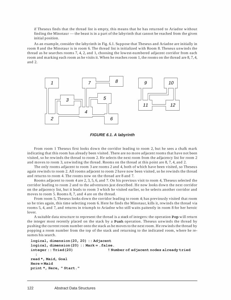
122
if Theseus finds that the thread list is empty, this means that he has returned to Ariadne withoutfinding the Minotaur — the beast is in a part of the labyrinth that cannot be reached from the giveninitial position.As an example, consider the labyrinth in Fig. 6.1. Suppose that Theseus and Ariadne are initially in
room 8 and the Minotaur is in room 6. The thread list is initialized with Room 8. Theseus unwinds thethread as he searches rooms 7, 4, 2, and 1, choosing the lowest-numbered adjacent corridor from eachroom and marking each room as he visits it. When he reaches room 1, the rooms on the thread are 8, 7, 4,and 2.
FIGURE 6.1. A labyrinth
From room 1 Theseus first looks down the corridor leading to room 2, but he sees a chalk markindicating that this room has already been visited. There are no more adjacent rooms that have not beenvisited, so he rewinds the thread to room 2. He selects the next room from the adjacency list for room 2and moves to room 3, unwinding the thread. Rooms on the thread at this point are 8, 7, 4, and 2.
The only rooms adjacent to room 3 are rooms 2 and 4, both of which have been visited, so Theseusagain rewinds to room 2. All rooms adjacent to room 2 have now been visited, so he rewinds the threadand returns to room 4. The rooms now on the thread are 8 and 7.
Rooms adjacent to room 4 are 2, 3, 5, 6, and 7. On his previous visit to room 4, Theseus selected thecorridor leading to room 2 and to the adventures just described. He now looks down the next corridoron the adjacency list, but it leads to room 3 which he visited earlier, so he selects another corridor andmoves to room 5. Rooms 8, 7, and 4 are on the thread.
From room 5, Theseus looks down the corridor leading to room 4; has previously visited that roomso he tries again, this time selecting room 6. Here he finds the Minotaur, kills it, rewinds the thread viarooms 5, 4, and 7, and returns in triumph to Ariadne who still waits paitently in room 8 for her heroiclover.
A suitable data structure to represent the thread is a stack of integers: the operation Pop will returnthe integer most recently placed on the stack by a Push operation. Theseus unwinds the thread bypushing the current room number onto the stack as he moves to the next room. He rewinds the thread bypopping a room number from the top of the stack and returning to the indicated room, where he re-sumes his search.
logical, dimension(20, 20) :: Adjacentlogical, dimension(20) :: Mark = .false.integer :: Tried(20) ! Number of adjacent nodes already tried
:read *, Maid, GoalHere = Maidprint *, Here, " Start."
1211
108 97
6
5
4
3
1
2
Abstract Data Structures
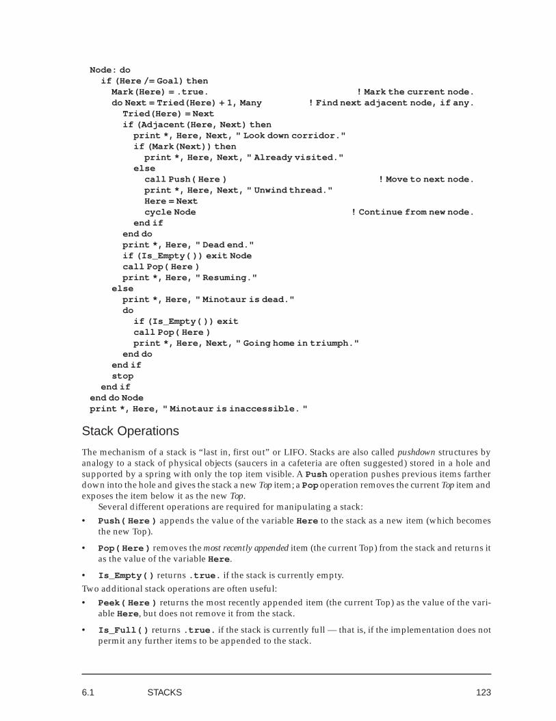
123
Node: doif (Here /= Goal) then
Mark(Here) = .true. ! Mark the current node.do Next = Tried(Here) + 1, Many ! Find next adjacent node, if any.
Tried(Here) = Nextif (Adjacent(Here, Next) then
print *, Here, Next, " Look down corridor."if (Mark(Next)) then
print *, Here, Next, " Already visited."else
call Push( Here ) ! Move to next node.print *, Here, Next, " Unwind thread."Here = Nextcycle Node ! Continue from new node.
end ifend doprint *, Here, " Dead end."if (Is_Empty( )) exit Nodecall Pop( Here )print *, Here, " Resuming."
elseprint *, Here, " Minotaur is dead."do
if (Is_Empty( )) exitcall Pop( Here )print *, Here, Next, " Going home in triumph."
end doend ifstop
end ifend do Nodeprint *, Here, " Minotaur is inaccessible. "
Stack Operations
The mechanism of a stack is “last in, first out” or LIFO. Stacks are also called pushdown structures byanalogy to a stack of physical objects (saucers in a cafeteria are often suggested) stored in a hole andsupported by a spring with only the top item visible. A Push operation pushes previous items fartherdown into the hole and gives the stack a new Top item; a Pop operation removes the current Top item andexposes the item below it as the new Top.
Several different operations are required for manipulating a stack:• Push( Here ) appends the value of the variable Here to the stack as a new item (which becomes
the new Top).
• Pop( Here ) removes the most recently appended item (the current Top) from the stack and returns itas the value of the variable Here .
• Is_Empty( ) returns .true. if the stack is currently empty.Two additional stack operations are often useful:• Peek( Here ) returns the most recently appended item (the current Top) as the value of the vari-
able Here , but does not remove it from the stack.
• Is_Full( ) returns .true. if the stack is currently full — that is, if the implementation does notpermit any further items to be appended to the stack.
6.1 STACKS
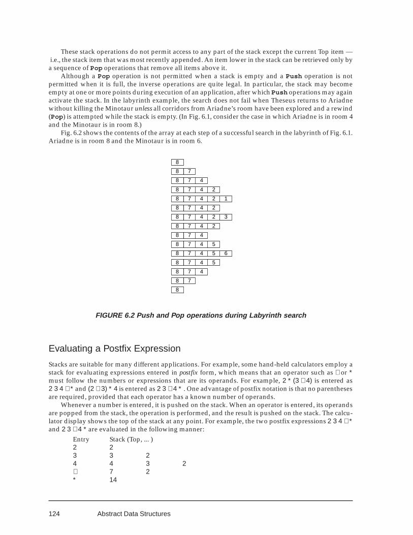
124
These stack operations do not permit access to any part of the stack except the current Top item —i.e., the stack item that was most recently appended. An item lower in the stack can be retrieved only bya sequence of Pop operations that remove all items above it.
Although a Pop operation is not permitted when a stack is empty and a Push operation is notpermitted when it is full, the inverse operations are quite legal. In particular, the stack may becomeempty at one or more points during execution of an application, after which Push operations may againactivate the stack. In the labyrinth example, the search does not fail when Theseus returns to Ariadnewithout killing the Minotaur unless all corridors from Ariadne’s room have been explored and a rewind(Pop) is attempted while the stack is empty. (In Fig. 6.1, consider the case in which Ariadne is in room 4and the Minotaur is in room 8.)
Fig. 6.2 shows the contents of the array at each step of a successful search in the labyrinth of Fig. 6.1.Ariadne is in room 8 and the Minotaur is in room 6.
FIGURE 6.2 Push and Pop operations during Labyrinth search
Evaluating a Postfix Expression
Stacks are suitable for many different applications. For example, some hand-held calculators employ astack for evaluating expressions entered in postfix form, which means that an operator such as + or ∗must follow the numbers or expressions that are its operands. For example, 2 ∗ (3 + 4) is entered as2 3 4 + ∗ and (2 + 3) ∗ 4 is entered as 2 3 + 4 ∗ . One advantage of postfix notation is that no parenthesesare required, provided that each operator has a known number of operands.
Whenever a number is entered, it is pushed on the stack. When an operator is entered, its operandsare popped from the stack, the operation is performed, and the result is pushed on the stack. The calcu-lator display shows the top of the stack at any point. For example, the two postfix expressions 2 3 4 + ∗and 2 3 + 4 ∗ are evaluated in the following manner:
Entry Stack (Top, ... )2 23 3 24 4 3 2+ 7 2∗ 14
8
78
478
2478
12478
2478
32478
2478
478
5478
65478
5478
478
78
8
Abstract Data Structures
125
2 23 3 2+ 54 4 5∗ 20
Stacks and Recursion
We have noted earlier that the activation record for a procedure contains space for local variables (ex-cept those for which space is reserved statically and those that are explicitly allocated in dynamic stor-age), for dummy argument values or their locations, for function result values, and for a few bytes ofinformation that are needed for returning execution control to the point from which the procedure wasreferenced. In the absence of recursion, only one copy of the activation record for each procedure isrequired, and some processors set aside space for all of these before execution of the main programbegins.
On the other hand, a procedure that calls itself recursively needs to save a copy of its activationrecord for each recursive call, so that the previous instance can be restored at exit. The usual implemen-tation of recursion employs a stack of activation records, sometimes called the central stack. The activa-tion record for each procedure (also called a stack frame) is pushed onto this stack at the time of proce-dure entry and is popped from the stack at procedure exit. While stack storage of activation records isalso possible for nonrecursive procedure calls, stack storage (or some other form of dynamic storage) isabsolutely essential for recursion because the depth of recursion and hence the number of activationrecords required cannot be predicted in advance.
The stack model is appropriate for activation record storage because procedure entry and exit al-ways conforms to a Last-In-First-Out (LIFO) discipline. However, the activation record stack fails in onerespect to conform to the usual definition of a stack, which permits access only to the top element. Incases such as inheritance by an internal procedure of a variable from its host, the currently executingprocedure makes reference to a local variable in a procedure whose activation record is not at the top ofthe stack.
Recursive Depth-First Search
The following recursive procedure corresponds to a part of the iterative program presented earlier. Herethe central stack performs the role of the programmed stack in the earlier example.
r ecursive subroutine Depth_First( Here )integer, intent (in) :: Here
integer :: Next! start subroutine Depth_First
Mark(Here) = .true. ! Mark the current node.if (Here /= Goal) then
!.. Find next unmarked adjacent node, if any.do Next = 1, Many
if (Adjacent(Here, Next) .and. .not. Mark(Next)) thencall Depth_First( Next ) ! Move to new node.if (Found) return
end ifend do
elseFound = .true.return
end ifreturn
end subroutine Labyrinth
6.1 STACKS
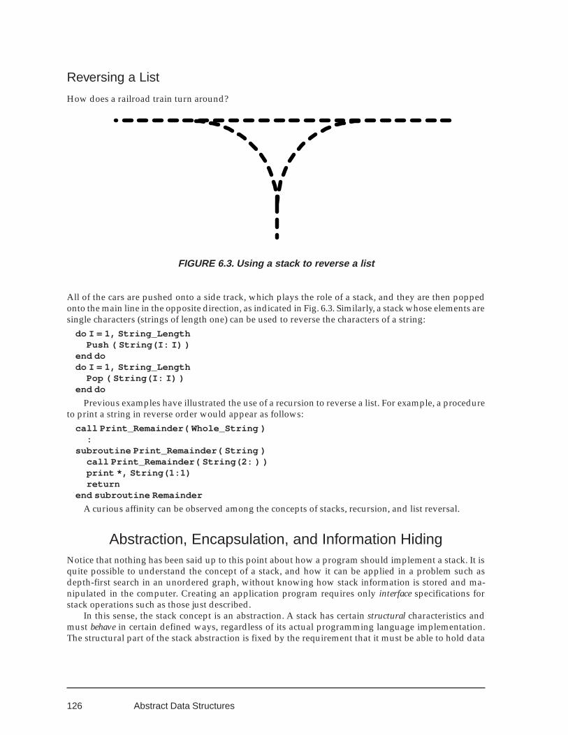
126
Reversing a List
How does a railroad train turn around?
Abstract Data Structures
FIGURE 6.3. Using a stack to reverse a list
All of the cars are pushed onto a side track, which plays the role of a stack, and they are then poppedonto the main line in the opposite direction, as indicated in Fig. 6.3. Similarly, a stack whose elements aresingle characters (strings of length one) can be used to reverse the characters of a string:
do I = 1, String_LengthPush ( String(I: I) )
end dodo I = 1, String_Length
Pop ( String(I: I) )end do
Previous examples have illustrated the use of a recursion to reverse a list. For example, a procedureto print a string in reverse order would appear as follows:
call Print_Remainder( Whole_String ):
subroutine Print_Remainder( String )call Print_Remainder( String(2: ) )print *, String(1:1)return
end subroutine Remainder
A curious affinity can be observed among the concepts of stacks, recursion, and list reversal.
Abstraction, Encapsulation, and Information HidingNotice that nothing has been said up to this point about how a program should implement a stack. It isquite possible to understand the concept of a stack, and how it can be applied in a problem such asdepth-first search in an unordered graph, without knowing how stack information is stored and ma-nipulated in the computer. Creating an application program requires only interface specifications forstack operations such as those just described.
In this sense, the stack concept is an abstraction. A stack has certain structural characteristics andmust behave in certain defined ways, regardless of its actual programming language implementation.The structural part of the stack abstraction is fixed by the requirement that it must be able to hold data
127
items of a certain type — for example, it may be a stack of integers, a stack of character strings of aspecific length, or a stack of structures of a particular derived type. The behavioral part is determined bya list of stack operations, with a precise description of the way in which each operation affects (or isaffected by) the stack.
Data abstraction — definition of the structure and behavior of an object, independent from itsimplementaion (as exemplified by the stack concept) — is a technique that has been shown to permitsignificant improvements in program design and reliability. Data abstraction and two other techniques,object encapsulation, and information hiding, are important principles in object design methodology.
Object encapsulation combines the structural and behavioral aspects of an object into a self-con-tained set of program statements. For encapsulation, Fortran provides modules that contain the datatype definitions and variable declarations for an abstract object, along with procedures that define eachof the required operations.
Information hiding protects the implementation from inadvertent modification by a consumer pro-gram. Some of the derived types and variables in the module are accessible to the consumer. The con-sumer also has access to interface information for the procedures that perform each of the requiredoperations. But derived types or their components, as well as the inner details of module procedures,can be made inaccessible from outside the module. The most important Fortran feature for informationhiding is the private declaration, which may appear in the specification part of a module with a list ofnames that are not to be imported when a use statement for the module appears in the main program orin a consumer module. Internal procedures within module subprograms are also automatically inacces-sible outside the module.
Consequently, a programming team can be organized so that consumers of an abstract object suchas a stack are insulated from the producers. The producers create a module to implement the Stackabstraction and they make it available (perhaps only in the form of compiled machine instructions) toconsumers along with written information concerning the external interface. Consumer programs callupon the module Stack to create objects and to perform operations on them but cannot modify or evenexamine Stack data except through the operations provided.
In a less formal environment, there may be only one programmer who wears two hats, sometimesacting as producer and sometimes as consumer. Nevertheless, a programmer can wear only one hat at atime and, while in the consumer role, must simulate information hiding by pretending to know only theexternal interface.
Stack as an ObjectA Stack can be implemented in any of several ways; the two most obvious implementations employ anarray or a linked list. The necessary type definitions, variable declarations, and procedure definitionsare encapsulated in a module that is imported to an application by a use statement.
The two following program examples present an array implementation module and a linked listimplementation module for the same Stack abstraction, along with a single main program that can useeither module. This demonstrates the possibility of constructing a Stack module so that a consumerwithout access to the source program cannot tell whether it employs an array or a linked list (exceptperhaps by some trick that might reveal the limited capacity of the former).
These two examples, and the other stack examples that follow, show the stack operations Push ,Pop, and Peek implemented as functions of logical type, omitting Is_Empty and Is_Full . Push re-turns .true. unless the stack is full (which, in the linked list versions, we assume cannot occur). Popand Peek return .true. unless the stack is empty; the top item is returned as an intent(out) argu-ment. Push , Pop, and Peek are not pure functions because they modify nonlocal data. In the examplesdistributed electronically, the subset versions implement these operations as subroutines (and includeseparate Is_Empty and Is_Full procedures), because neither subset permits intent(out) functionarguments.
6.1 STACKS
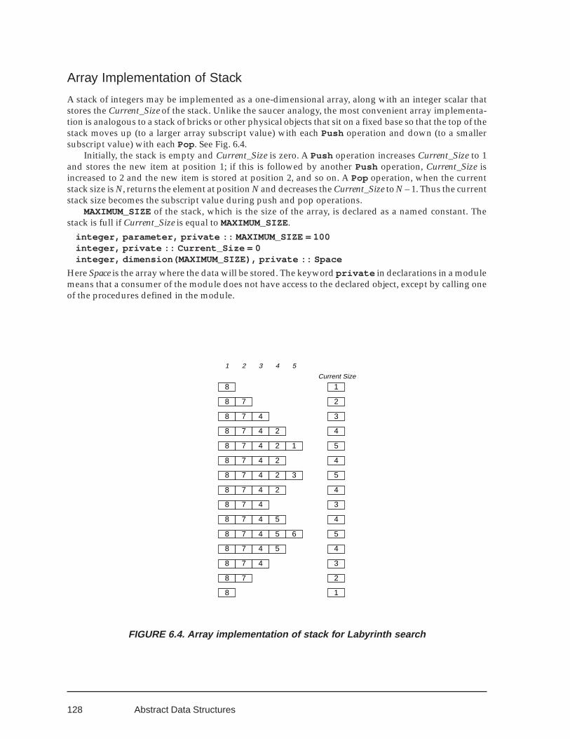
128
Array Implementation of Stack
A stack of integers may be implemented as a one-dimensional array, along with an integer scalar thatstores the Current_Size of the stack. Unlike the saucer analogy, the most convenient array implementa-tion is analogous to a stack of bricks or other physical objects that sit on a fixed base so that the top of thestack moves up (to a larger array subscript value) with each Push operation and down (to a smallersubscript value) with each Pop. See Fig. 6.4.
Initially, the stack is empty and Current_Size is zero. A Push operation increases Current_Size to 1and stores the new item at position 1; if this is followed by another Push operation, Current_Size isincreased to 2 and the new item is stored at position 2, and so on. A Pop operation, when the currentstack size is N, returns the element at position N and decreases the Current_Size to N – 1. Thus the currentstack size becomes the subscript value during push and pop operations.
MAXIMUM_SIZE of the stack, which is the size of the array, is declared as a named constant. Thestack is full if Current_Size is equal to MAXIMUM_SIZE.
integer, parameter, private :: MAXIMUM_SIZE = 100integer, private :: Current_Size = 0integer, dimension(MAXIMUM_SIZE), private :: Space
Here Space is the array where the data will be stored. The keyword private in declarations in a modulemeans that a consumer of the module does not have access to the declared object, except by calling oneof the procedures defined in the module.
Abstract Data Structures
8
1 2 3 4 5
8 7
8 7 4
8 7 4 2
8 7 4 2
8 7 4 2 3
8 7 4 2
8 7 4
8 7 4 5
8 7 4 5 6
8 7 4 5
8 7 4
8 7
8
1
2
3
4
4
5
4
3
4
5
4
3
2
1
8 7 4 2 1 5
Current Size
FIGURE 6.4. Array implementation of stack for Labyrinth search
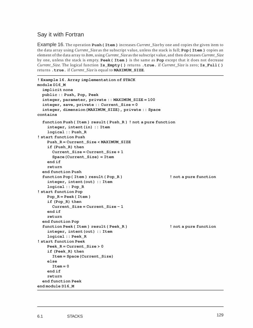
129
Say it with Fortran
Example 16. The operation Push( Item ) increases Current_Size by one and copies the given item tothe data array using Current_Size as the subscript value, unless the stack is full; Pop( Item ) copies anelement of the data array to Item, using Current_Size as the subscript value, and then decreases Current_Sizeby one, unless the stack is empty. Peek( Item ) is the same as Pop except that it does not decreaseCurrent_Size. The logical function Is_Empty( ) returns .true. if Current_Size is zero; Is_Full( )returns .true. if Current_Size is equal to MAXIMUM_SIZE.
! Example 16. Array implementation of STACKmodule D16_M
implicit nonepublic :: Push, Pop, Peekinteger, parameter, private :: MAXIMUM_SIZE = 100integer, save, private :: Current_Size = 0integer, dimension(MAXIMUM_SIZE), private :: Space
contains
function Push( Item ) result( Push_R ) ! not a pure functioninteger, intent(in) :: Itemlogical :: Push_R
! start function PushPush_R = Current_Size < MAXIMUM_SIZEif (Push_R) then
Current_Size = Current_Size + 1Space(Current_Size) = Item
end ifreturn
end function Pushfunction Pop( Item ) result( Pop_R ) ! not a pure function
integer, intent(out) :: Itemlogical :: Pop_R
! start function PopPop_R = Peek( Item )if (Pop_R) then
Current_Size = Current_Size - 1end ifreturn
end function Popfunction Peek( Item ) result( Peek_R ) ! not a pure function
integer, intent(out) :: Itemlogical :: Peek_R
! start function PeekPeek_R = Current_Size > 0if (Peek_R) then
Item = Space(Current_Size)else
Item = 0end ifreturn
end function Peekend module D16_M
6.1 STACKS
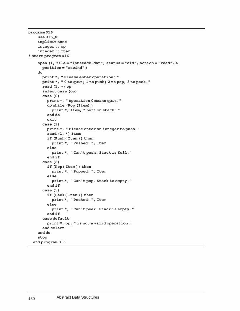
130
program D16use D16_Mimplicit noneinteger :: opinteger :: Item
! start program D16
open (1, file = "intstack.dat", status = "old", action = "read", &position = "rewind" )
doprint *, " Please enter operation: "print *, " 0 to quit; 1 to push; 2 to pop, 3 to peek."read (1, *) opselect case (op)case (0)
print *, " operation 0 means quit."do while (Pop (Item) )
print *, Item, " Left on stack. "end doexit
case (1)print *, " Please enter an integer to push."read (1, *) Itemif (Push( Item )) then
print *, " Pushed: ", Itemelse
print *, " Can't push. Stack is full."end if
case (2)if (Pop( Item )) then
print *, " Popped: ", Itemelse
print *, " Can't pop. Stack is empty."end if
case (3)if (Peek( Item )) then
print *, " Peeked: ", Itemelse
print *, " Can't peek. Stack is empty."end if
case defaultprint *, op, " is not a valid operation."
end selectend dostop
end program D16
Abstract Data Structures
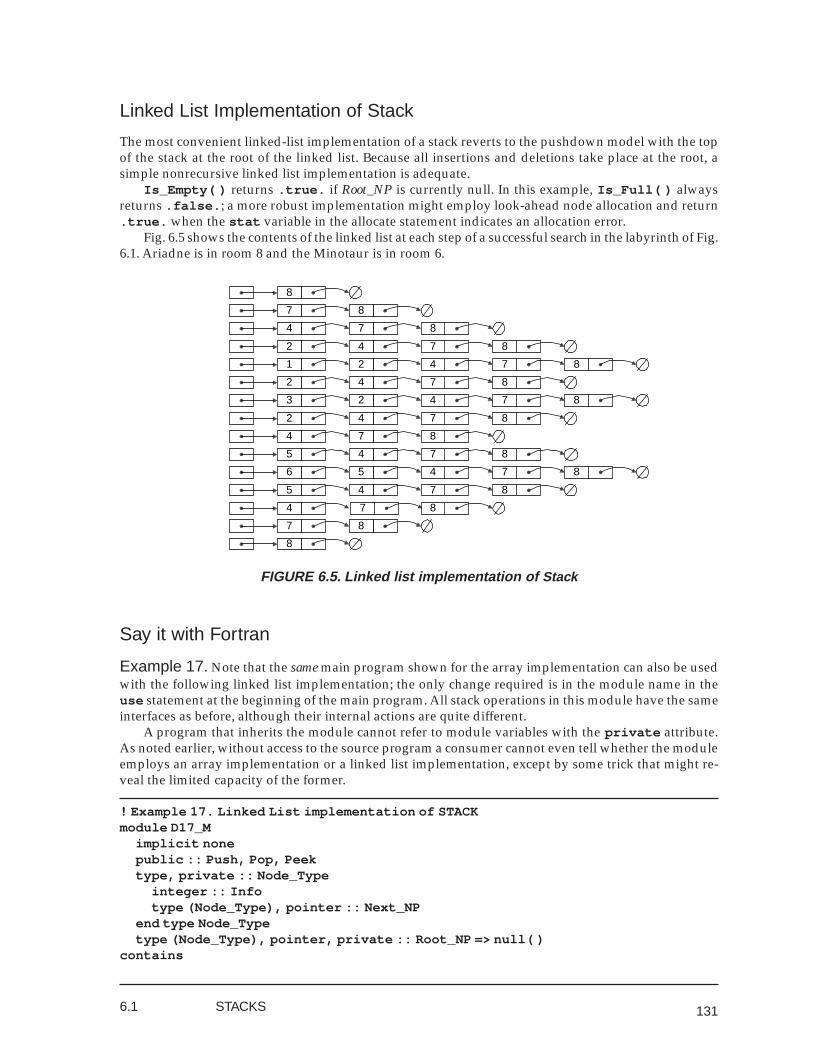
1316.1 STACKS
8745
87456
8745
8
87
874
8
87
874
8742
87421
8742
87423
8742
874
Linked List Implementation of Stack
The most convenient linked-list implementation of a stack reverts to the pushdown model with the topof the stack at the root of the linked list. Because all insertions and deletions take place at the root, asimple nonrecursive linked list implementation is adequate.
Is_Empty( ) returns .true. if Root_NP is currently null. In this example, Is_Full( ) alwaysreturns .false. ; a more robust implementation might employ look-ahead node allocation and return.true. when the stat variable in the allocate statement indicates an allocation error.
Fig. 6.5 shows the contents of the linked list at each step of a successful search in the labyrinth of Fig.6.1. Ariadne is in room 8 and the Minotaur is in room 6.
FIGURE 6.5. Linked list implementation of Stack
Say it with Fortran
Example 17. Note that the same main program shown for the array implementation can also be usedwith the following linked list implementation; the only change required is in the module name in theuse statement at the beginning of the main program. All stack operations in this module have the sameinterfaces as before, although their internal actions are quite different.
A program that inherits the module cannot refer to module variables with the private attribute.As noted earlier, without access to the source program a consumer cannot even tell whether the moduleemploys an array implementation or a linked list implementation, except by some trick that might re-veal the limited capacity of the former.
! Example 17. Linked List implementation of STACKmodule D17_M
implicit nonepublic :: Push, Pop, Peektype, private :: Node_Type
integer :: Infotype (Node_Type), pointer :: Next_NP
end type Node_Typetype (Node_Type), pointer, private :: Root_NP => null( )
contains
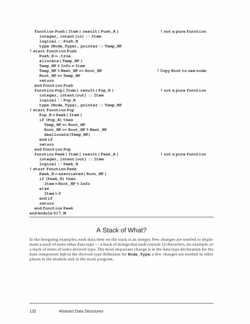
132
function Push( Item ) result( Push_R ) ! not a pure functioninteger, intent(in) :: Itemlogical :: Push_Rtype (Node_Type), pointer :: Temp_NP
! start function PushPush_R = .true.allocate( Temp_NP )Temp_NP % Info = ItemTemp_NP % Next_NP => Root_NP ! Copy Root to new nodeRoot_NP => Temp_NPreturn
end function Pushfunction Pop( Item ) result( Pop_R ) ! not a pure function
integer, intent(out) :: Itemlogical :: Pop_Rtype (Node_Type), pointer :: Temp_NP
! start function PopPop_R = Peek( Item )if (Pop_R) then
Temp_NP => Root_NPRoot_NP => Root_NP % Next_NPdeallocate(Temp_NP)
end ifreturn
end function Popfunction Peek( Item ) result( Peek_R ) ! not a pure function
integer, intent(out) :: Itemlogical :: Peek_R
! start function PeekPeek_R = associated( Root_NP )if (Peek_R) then
Item = Root_NP % Infoelse
Item = 0end ifreturn
end function Peekend module D17_M
A Stack of What?In the foregoing examples, each data item on the stack is an integer. Few changes are needed to imple-ment a stack of some other data type — a stack of strings that each contain 12 characters, for example, ora stack of items of some derived type. The most important change is in the data type declaration for thedata component Info in the derived type definition for Node_Type ; a few changes are needed in otherplaces in the module and in the main program.
Abstract Data Structures
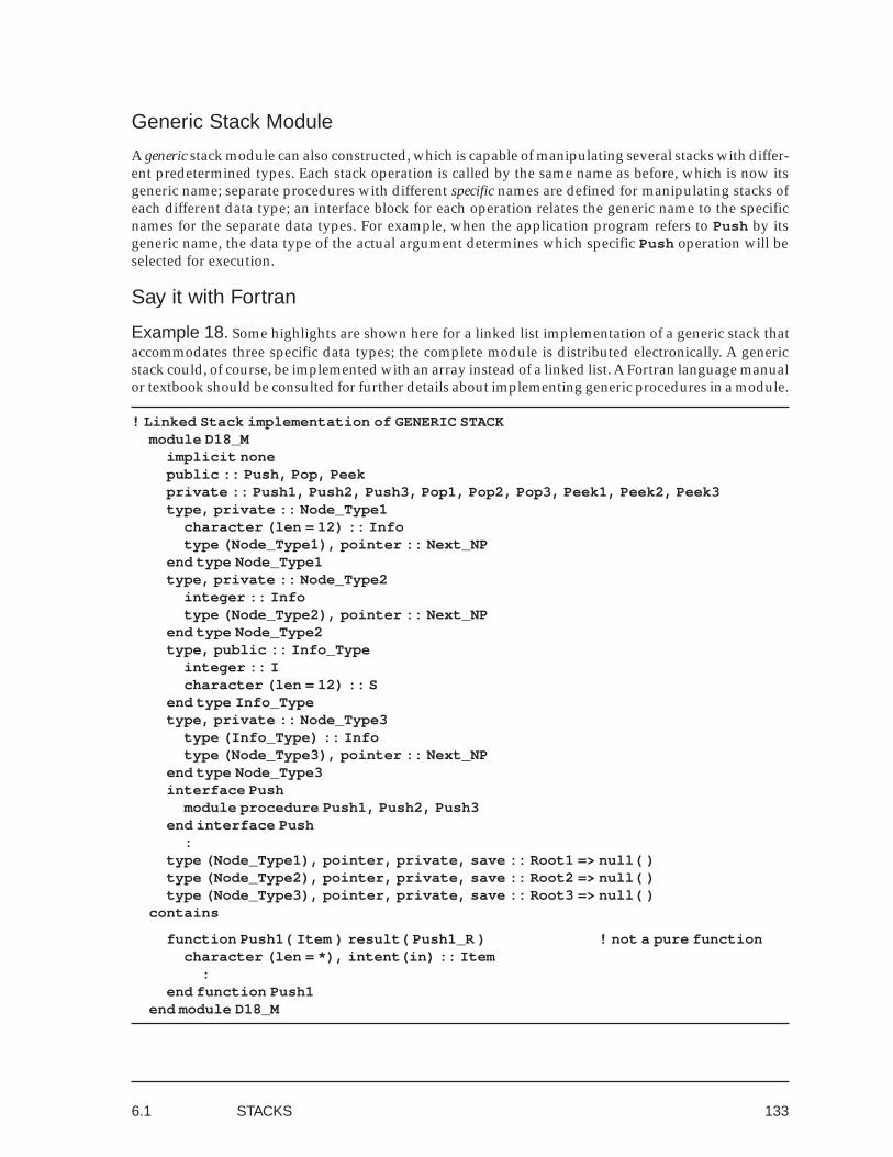
133
Generic Stack Module
A generic stack module can also constructed, which is capable of manipulating several stacks with differ-ent predetermined types. Each stack operation is called by the same name as before, which is now itsgeneric name; separate procedures with different specific names are defined for manipulating stacks ofeach different data type; an interface block for each operation relates the generic name to the specificnames for the separate data types. For example, when the application program refers to Push by itsgeneric name, the data type of the actual argument determines which specific Push operation will beselected for execution.
Say it with Fortran
Example 18. Some highlights are shown here for a linked list implementation of a generic stack thataccommodates three specific data types; the complete module is distributed electronically. A genericstack could, of course, be implemented with an array instead of a linked list. A Fortran language manualor textbook should be consulted for further details about implementing generic procedures in a module.
! Linked Stack implementation of GENERIC STACKmodule D18_M
implicit nonepublic :: Push, Pop, Peekprivate :: Push1, Push2, Push3, Pop1, Pop2, Pop3, Peek1, Peek2, Peek3type, private :: Node_Type1
character (len = 12) :: Infotype (Node_Type1), pointer :: Next_NP
end type Node_Type1type, private :: Node_Type2
integer :: Infotype (Node_Type2), pointer :: Next_NP
end type Node_Type2type, public :: Info_Type
integer :: Icharacter (len = 12) :: S
end type Info_Typetype, private :: Node_Type3
type (Info_Type) :: Infotype (Node_Type3), pointer :: Next_NP
end type Node_Type3interface Push
module procedure Push1, Push2, Push3end interface Push
:type (Node_Type1), pointer, private, save :: Root1 => null( )type (Node_Type2), pointer, private, save :: Root2 => null( )type (Node_Type3), pointer, private, save :: Root3 => null( )
contains
function Push1( Item ) result( Push1_R ) ! not a pure functioncharacter (len = *), intent(in) :: Item
:end function Push1
end module D18_M
6.1 STACKS
134
program D18use D18_Mimplicit nonecharacter (len = 12) :: Item1integer :: Item2type (Info_Type) :: Item3
! start program E18
if (Push( "ABCDEFGHIJKL" )) print *, " Push: ABCDEFGHIJKL"if (Push( 11111 )) print *, " Push: 11111"if (Push( Info_Type( 11, "Hello world.") )) print *, " Push: 11 Hello world."
:
Here three stacks are defined with different node types, each having a different Info component datatype. Based on the node type of the actual argument data item in each call to the generic proceduresPush , Pop, or Peek , the module resolves the generic reference and selects one of the specific procedures.
Push and Pop operations with items of different data types can be intermixed; each operation willautomatically select the specific stack appropriate to the data type of the actual argument item. A Popoperation will return the latest pushed item from the corresponding stack, even though items of othertypes may have been pushed on the other stacks in the meantime.
Stack ObjectsIn the foregoing examples a single stack (or in the generic example a single stack for each supported datatype) is declared in the module. The main program does not specify a particular stack that is to beoperated upon.
For some applications, it may be preferable to permit the application program to create more thanone stack and to designate a specific stack at each reference to an operation. Deferring, for the moment,discussion of generic stacks, we now assume a fixed node type with a data component of type Info_Type .
The main program for an array implementation could include declarations such asinteger, parameter :: MAXIMUM_SIZE1 = 100integer :: Current_Size1 = 0integer, dimension(MAXIMUM_SIZE1) :: Space1 = 0
while the main program for a linked list implementation would declare a root pointer such astype (Node_Type), pointer :: Root_NP1 => Null( )
STOP! Whatever happened to information hiding?This approach clearly violates the principles of data abstraction. Although stack operations are still
combined in a module, the data structure is no longer encapsulated — it is declared in the main programwhere it is fully accessible and can be changed in ways that might violate the integrity of the moduleprocedures.
Abstract Data Structures
32 Versions prior to Fortran 95 nullify the root pointer.
135
Instead, the module should declare a Stack_Type , whose inner details will vary according to theimplementation. For an array implementation:
integer, parameter, private :: M = 100type, public :: Stack_Type
privateinteger, private :: Maximum_Size = M, Current_Size = 0character (len = 12), pointer, dimension(:) :: Space
end type Stack_Type
and for a linked list implementation:type, public :: Stack_Type
privatetype (Node_Type), pointer :: Root_NP => Null( )
end type Stack_Type
For each different stack, a declaration in the application program creates an object of Stack_Typeaccording to the derived type definition in the module, whose components are inaccessible because ofthe private specification. This declared object can be passed as an actual argument to any of the stackoperations defined in the module. A module procedure Create_Stack , with a dummy argument oftype Stack_Type , allocates the Space array for an array implementation but does essentially nothingfor a linked list implementation.32 Delete_Stack terminates the lifetime of a particular stack anddeallocates any space that was allocated for the stack by Create_Stack .
! Array implementationsubroutine Create_Stack( Arg_S )
type (Stack_Type), intent(in out) :: Arg_S! start subroutine Create_Stack
allocate( Arg_S % Space(100))Arg_S % Space = " "return
end subroutine Create_Stack
! Linked list implementationsubroutine Create_Stack( Arg_S )
type (Stack_Type), intent(in out) :: Arg_S! start subroutine Create_Stack
returnend subroutine Create_Stack
! MAIN PROGRAMtype (Info_Type) :: Itemtype (Stack_Type) :: Stack
:call Create_Stack( Stack )Item = Info_Type( "ABCDEFGHIJKL" )if (Push( Stack, Item )) print *, Item
:call Destroy_Stack( Stack )
The consumer will need to be aware of the structure of Info_Type so that items to be pushed onto thestack can be generated properly.
6.1 STACKS
136
Say it with Fortran
Example 19. The main program contains declarations for objects of two different types: a stack objectof type Stack_Type and a data item of type Info_Type . The create and destroy operations are notshown here.
! Linked Stack implementation of STACK OBJECTmodule D19_M
implicit nonepublic :: Push, Pop, Peektype, public :: Info_Type
character (len = 12) :: Send type Info-Typetype, private :: Node_Type
type (Info-Type) :: Infotype (Node_Type), pointer :: Next_NP
end type Node_Typetype, public :: Stack_Type
privatetype (Node_Type), pointer :: Root_NP
end type Stack_Typecontains
function Push( Arg_SP, Item ) result( Push_R ) ! not a pure functiontype (Stack_Type), intent(in out) :: Arg_SPtype (Info_Type), intent(in) :: Itemlogical :: Push_Rtype (Node_Type), pointer :: Temp_NP
! start function PushPush_R = .true.allocate( Temp_NP )Temp_NP % Info = ItemTemp_NP % Next_NP => Arg_SP % Root_NP ! Copy Root to new nodeArg_SP % Root_NP => Temp_NPreturn
end function Pushfunction Pop( Arg_SP, Item ) result( Pop_R ) ! not a pure function
type (Stack_Type), intent(in out) :: Arg_SPtype (Info-Type), intent(out) :: Itemlogical :: Pop_Rtype (Node_Type), pointer :: Temp_NP
! start function PopPop_R = Peek( Arg_SP, Item )if (Pop_R) then
Temp_NP => Arg_SP % Root_NPArg_SP % Root_NP => Arg_SP % Root_NP % Next_NPdeallocate( Temp_NP )
end ifreturn
end function Pop
Abstract Data Structures
137
function Peek( Arg_SP, Item ) result( Peek_R ) ! not a pure functiontype (Stack_Type), intent(in) :: Arg_SPlogical :: Peek_Rtype (Info-Type), intent(out) :: Item
! start function PeekPeek_R = associated( Arg_SP % Root_NP )if (Peek_R) then
Item = Arg_SP % Root_NP % Infoelse
Item = Info_Type( "" )end ifreturn
end function Peekend module D19_M
Extension to a generic module for stack objects requires a separate stack type for each stack dataitem type, along with a separate set of specific stack procedures for each stack type (as before). Theconsumer declares objects of various specific stack types as required and calls stack operation proce-dures by their generic names such as Create_Stack , Push , and Pop.
6.2 QUEUESQueue is a French word meaning tail. The word in English is applied to waiting lines, which are sup-posed to resemble a tail. A familiar queue is the checkout line in a supermarket where customers withtheir shopping carts wait to pay for their groceries.
A queue is a list that operates according to a first-in, first-out (FIFO) discipline. Items (such as cus-tomers) enter the queue at one end and exit at the other end — in contrast to a LIFO stack where itemsenter and exit at the same end. The queue operations Enqueue (for entering the queue) and Dequeue(for leaving the queue) correspond to the stack operations Push and Pop. As in a waiting line, itemsleave (Dequeue ) at the front of a queue and they enter (Enqueue ) at the rear.
Six queue operations are considered here, corresponding to the seven stack operations with theomission of Peek .• Create_Queue( ) allocates space for the queue and marks it as empty.
• Delete_Queue( ) removes any remaining items from the queue and releases the space that wasallocated for it.
• Enqueue( Item ) appends Item to the contents of the queue.
• Dequeue( Item ) removes the least recently appended integer from the queue and returns it as thevalue of Item .
• Is_Empty( ) returns .true. if the queue is currently empty.
• Is_Full( ) returns .true. if the queue is currently full — that is, if the implementation does notpermit any further items to be appended to the queue.Dequeue operations are not permitted when a queue is empty and Enqueue operations are not
permitted when it is full, but the inverse operations are quite legal. In particular, the queue may becomeempty at one or more points during execution of an application, after which Enqueue operations mayagain produce a nonempty queue.
6.2 QUEUES
138
Jones Brown
Rear of Queue
Rear Pointer
Root Box
Jones
Rear of Queue
Rear Pointer
Root Box
Rear Pointer
Root Box
Abstract Data Structures
Queue ObjectsA queue can be implemented with an array or with a linked list. In either case, the necessary typedefinitions, variable declarations, and procedure definitions are encapsulated in a module that is im-ported to an application by a use statement. Queues in the following examples hold character strings oflength 12; queues for data of other intrinsic or derived types, as well as generic queues and allocatedqueues, are of course also possible.
The following program examples present both an array implementation and a linked list implemen-tation for the same queue abstraction. Thus they show that it is possible to construct a queue module sothat a consumer without access to the source program cannot tell (except by trickery) whether it em-ploys a linked list or an array.
Linked List Implementation of Queue
A queue may be implemented as a linked list, with one end of the queue at the root and the other end atthe tail. Which end of the queue should be at the root of the linked list?
An operation for repeatedly deleting the tail node from a linked list would be difficult to implement(without some enhancement such as the bidirectional pointers of a doubly-linked list; see Sec. 5.4), for thefollowing reason: To avoid searching through the entire list at each deletion, an extra pointer to the tailnode is required. Deleting the current tail node from a linked list moves the tail pointer to the predeces-sor node, but there is no straightforward way to find the predecessor of the current target of a nodepointer in a singly-linked list. Therefore, the tail of the linked list should correspond to the rear of thequeue where insertions (Enqueue operations) occur; it follows that the root of the linked list shouldcorrespond to the front of the queue where deletions (Dequeue operations) occur.
A bit of complication is still required for the Enqueue operation — that is, for inserting a new nodeat the tail of a linked list and updating the queue rear pointer. In the obvious implementation, the targetof the queue rear pointer should always be the current tail node in the linked list, but there is no suchnode when the linked list is empty.
FIGURE 6.6. Pointer to Pointer implementation of Enqueue
139
Say it with Fortran
Example 20. The implementation given here employs the Pointer to Pointer strategy mentioned ear-lier: each node pointer (that is, the Root pointer as well as the Next_NP component in each node) isreplaced by a pointer to this node pointer, implemented in Fortran as a pointer to a BOX structure whoseonly component is the node pointer. In this implementation the queue rear is a BOX pointer whose targetis either the BOX component of the tail node in the linked list or (if the linked list is empty) the root BOX,as shown in Fig. 6.6.
A Dequeue operation deletes the current root node, which is the target of Root % Next_NP . This isthe usual Delete_Node linked list operation except when there is only one item in the queue; in thatcase, deleting the root node also deletes the tail node so the Dequeue operation must modify the queuerear pointer Tail_BP as well as Root.
Create_Queue nullifies the node pointer component of Root and makes Root the target of Tail_BP.
! Example 20. Linked List (Pointer to Pointer) implementation of QUEUE OBJECTmodule D20_M
implicit nonepublic :: Create_Queue, Destroy_Queue, Enqueue, Dequeue, &
Is_Empty, Is_Full
type, private :: BOX_Typetype (Node_Type), pointer :: Next_NP => Null( )
end type BOX_Type
type, private :: Node_Typecharacter (len = 12) :: Infotype (BOX_Type) :: BOX
end type Node_Type
type, public :: Queue_Typeprivate
type (BOX_Type) :: Roottype (BOX_Type), pointer :: Tail_BP => null( )end type Queue_Type
contains
subroutine Create_Queue( Arg_Q )type (Queue_Type), target, intent(in out) :: Arg_Q
! start subroutine Create_QueueArg_Q % Tail_BP => Arg_Q % Rootreturn
end subroutine Create_Queue
subroutine Destroy_Queue( Arg_Q )type (Queue_Type), intent(in out) :: Arg_Qcharacter (len = 12) :: Info
! start subroutine Destroy_Queuedo while (.not. Is_Empty( Arg_Q ))
call Dequeue( Arg_Q, Info )print *, " Left on Queue: ", Info
end doreturn
end subroutine Destroy_Queue
6.2 QUEUES
140
subroutine Enqueue( Arg_Q, Item )type (Queue_Type), intent(in out) :: Arg_Qcharacter (len = 12), intent(in) :: Itemtype (Node_Type), pointer :: Temp_NP
! start subroutine Enqueueallocate( Temp_NP )Temp_NP % Info = ItemArg_Q % Tail_BP % Next_NP => Temp_NP ! Link new node into list.Arg_Q % Tail_BP => Temp_NP % BOX ! New node becomes new tail.
! nullify( Temp_NP )return
end subroutine Enqueue
subroutine Dequeue( Arg_Q, Item )type (Queue_Type), target, intent(in out) :: Arg_Qcharacter (len = *), intent(out) :: Itemtype (Node_Type), pointer :: Temp_NP
! start subroutine Dequeueif (Is_Empty( Arg_Q )) then
print *, " Attempt to pop from empty stack. "Item = " "
elseTemp_NP => Arg_Q % Root % Next_NPItem = Temp_NP % InfoArg_Q % Root = Temp_NP % BOXdeallocate( Temp_NP )if (Is_Empty( Arg_Q )) Arg_Q % Tail_BP => Arg_Q % Root
end ifreturn
end subroutine Dequeue
pure function Is_Empty( Arg_Q ) result( X )type (Queue_Type), intent(in out) :: Arg_Qlogical :: X
! start function Is_EmptyX = (.not. associated (Arg_Q % Root % Next_NP))return
end function Is_Empty
pure function Is_Full( Arg_Q ) result( X )type (Queue_Type), intent(in out) :: Arg_Qlogical :: X
! start function Is_FullX = .false.return
end function Is_Full
end module D20_M
program D20use D20_Mimplicit noneinteger :: Opcharacter (len = 12) :: Item = " "type(Queue_Type) :: Queue
! start program D20
Abstract Data Structures
141
call Create_Queue ( Queue )do
print *, " Please enter Operation: "print *, " 0 to quit; 1 to enqueue; 2 to dequeue."read *, Opselect case (Op)case (0)
print *, " Operation 0 means quit."exit
case (1)if (Is_Full( Queue )) then
print *, " Can't enqueue. Queue is full. "else
print *, " Please enter an item to enqueue."read *, Itemcall Enqueue( Queue, Item )print *, " Enqueued: ", Item
end ifcase (2)
if (Is_Empty( Queue )) thenprint *, " Can't dequeue. Queue is empty. "
elsecall Dequeue( Queue, Item )print *, " Dequeued: ", Item
end ifcase default
print *, Op, " is not a valid operation."end select
end docall Destroy_Queue( Queue )stop
end program D20
Array Implementation of Queue
An important queue application in computer systems is input and output buffering, motivated by theslow execution speed of external data transmission. When an input file is opened, data is transmittedfrom the file and is enqueued in an input buffer, to be dequeued during execution of a read statement.Write statements enqueue data in an output buffer, from which it is written to the file as a separate opera-tion while program execution proceeds. For maximum efficiency, these buffers are traditionally imple-mented as one-dimensional arrays.
Although the customers in a supermarket queue move toward the front of the queue each time aDequeue operation occurs, queues implemented as arrays avoid the inefficiency that such moves wouldentail. Each data item remains in a fixed position during queue operations, while front and rear queueposition marker values change. The rear position is incremented when an item is enqueued; the frontposition is incremented when an item is dequeued.
In a typical queue, only a few items are stored at one time, while the total number of items that passthrough the queue during an interval is many times larger. Someone long ago discovered how to main-tain a queue with an array just big enough to hold the maximum number of concurrently stored items. Itis not necessary to allocate separate space for all the items that pass through the queue — array space isnot needed for items that have not yet been enqueued or for those that have already been dequeued.
Queues used for input or output are traditionally described as circular buffers, because their arraysubscripts are kept within bounds by applying a circular transformation — that is, by reducing the sub-
6.2 QUEUES
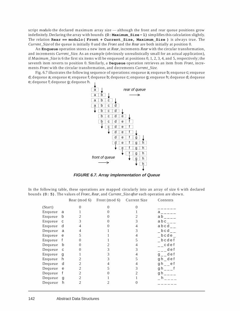
142 Abstract Data Structures
h
ba
cba
dcba
dcb
edcb
fedcb
fedc
fed
gfed
hgfed
hgfe
hgf
hg
a
front of queue
rear of queue
script modulo the declared maximum array size — although the front and rear queue positions growindefinitely. Declaring the array with bounds (0: Maximum_Size – 1) simplifies this calculation slightly.The relation Rear == modulo( Front + Current_Size, Maximum_Size ) is always true. TheCurrent_Size of the queue is initially 0 and the Front and the Rear are both initially at position 0.
An Enqueue operation stores a new item at Rear, increments Rear with the circular transformation,and increments Current_Size. As an example (obviously unrealistically small for an actual application),if Maximum_Size is 6 the first six items will be enqueued at positions 0, 1, 2, 3, 4, and 5, respectively; theseventh item reverts to position 0. Similarly, a Dequeue operation retrieves an item from Front, incre-ments Front with the circular transformation, and decrements Current_Size.
Fig. 6.7 illustrates the following sequence of operations: enqueue a; enqueue b; enqueue c; enqueued; dequeue a; enqueue e; enqueue f; dequeue b; dequeue c; enqueue g; enqueue h; dequeue d; dequeuee; dequeue f; dequeue g; dequeue h.
FIGURE 6.7. Array implementation of Queue
In the following table, these operations are mapped circularly into an array of size 6 with declaredbounds (0: 5) . The values of Front, Rear, and Current_Size after each operation are shown.
Rear (mod 6) Front (mod 6) Current Size Contents
(Start) 0 0 0 _ _ _ _ _ _Enqueue a 1 0 1 a _ _ _ _ _Enqueue b 2 0 2 a b _ _ _ _Enqueue c 3 0 3 a b c _ _ _Enqueue d 4 0 4 a b c d _ _Dequeue a 4 1 3 _ b c d _ _Enqueue e 5 1 4 _ b c d e _Enqueue f 0 1 5 _ b c d e fDequeue b 0 2 4 _ _ c d e fDequeue c 0 3 3 _ _ _ d e fEnqueue g 1 3 4 g _ _ d e fEnqueue h 2 3 5 g h _ d e fDequeue d 2 4 4 g h _ _ e fDequeue e 2 5 3 g h _ _ _ fDequeue f 2 0 2 g h _ _ _ _Dequeue g 2 1 1 _ h _ _ _ _Dequeue h 2 2 0 _ _ _ _ _ _
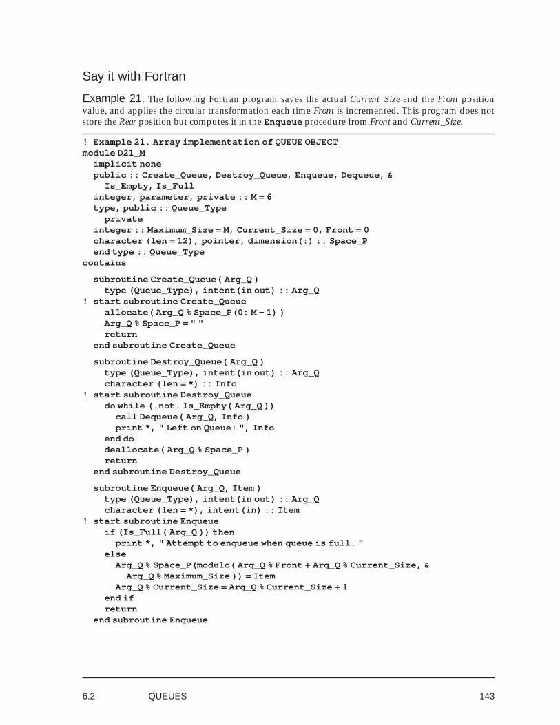
143
Say it with Fortran
Example 21. The following Fortran program saves the actual Current_Size and the Front positionvalue, and applies the circular transformation each time Front is incremented. This program does notstore the Rear position but computes it in the Enqueue procedure from Front and Current_Size.
! Example 21. Array implementation of QUEUE OBJECTmodule D21_M
implicit nonepublic :: Create_Queue, Destroy_Queue, Enqueue, Dequeue, &
Is_Empty, Is_Fullinteger, parameter, private :: M = 6type, public :: Queue_Type
privateinteger :: Maximum_Size = M, Current_Size = 0, Front = 0character (len = 12), pointer, dimension(:) :: Space_Pend type :: Queue_Type
contains
subroutine Create_Queue( Arg_Q )type (Queue_Type), intent(in out) :: Arg_Q
! start subroutine Create_Queueallocate( Arg_Q % Space_P(0: M - 1) )Arg_Q % Space_P = " "return
end subroutine Create_Queue
subroutine Destroy_Queue( Arg_Q )type (Queue_Type), intent(in out) :: Arg_Qcharacter (len = *) :: Info
! start subroutine Destroy_Queuedo while (.not. Is_Empty( Arg_Q ))
call Dequeue( Arg_Q, Info )print *, " Left on Queue: ", Info
end dodeallocate( Arg_Q % Space_P )return
end subroutine Destroy_Queue
subroutine Enqueue( Arg_Q, Item )type (Queue_Type), intent(in out) :: Arg_Qcharacter (len = *), intent(in) :: Item
! start subroutine Enqueueif (Is_Full( Arg_Q )) then
print *, " Attempt to enqueue when queue is full. "else
Arg_Q % Space_P(modulo( Arg_Q % Front + Arg_Q % Current_Size, &Arg_Q % Maximum_Size )) = Item
Arg_Q % Current_Size = Arg_Q % Current_Size + 1end ifreturn
end subroutine Enqueue
6.2 QUEUES
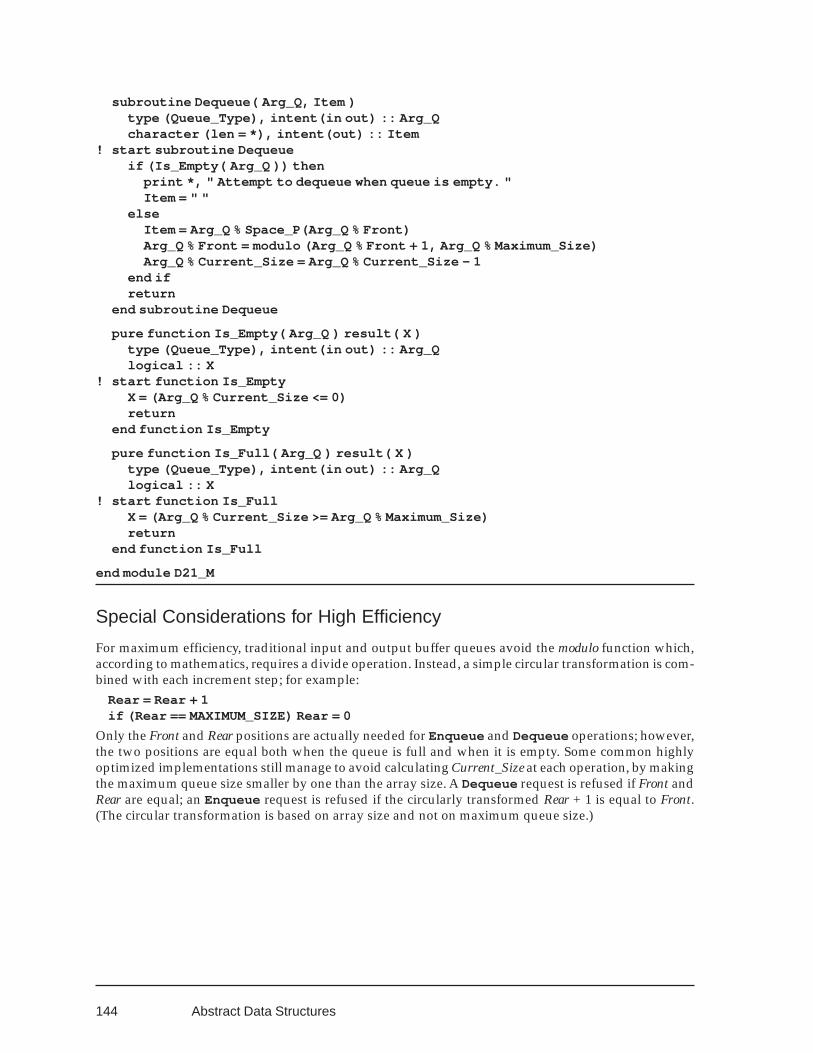
144
subroutine Dequeue( Arg_Q, Item )type (Queue_Type), intent(in out) :: Arg_Qcharacter (len = *), intent(out) :: Item
! start subroutine Dequeueif (Is_Empty( Arg_Q )) then
print *, " Attempt to dequeue when queue is empty. "Item = " "
elseItem = Arg_Q % Space_P(Arg_Q % Front)Arg_Q % Front = modulo (Arg_Q % Front + 1, Arg_Q % Maximum_Size)Arg_Q % Current_Size = Arg_Q % Current_Size - 1
end ifreturn
end subroutine Dequeue
pure function Is_Empty( Arg_Q ) result( X )type (Queue_Type), intent(in out) :: Arg_Qlogical :: X
! start function Is_EmptyX = (Arg_Q % Current_Size <= 0)return
end function Is_Empty
pure function Is_Full( Arg_Q ) result( X )type (Queue_Type), intent(in out) :: Arg_Qlogical :: X
! start function Is_FullX = (Arg_Q % Current_Size >= Arg_Q % Maximum_Size)return
end function Is_Full
end module D21_M
Special Considerations for High Efficiency
For maximum efficiency, traditional input and output buffer queues avoid the modulo function which,according to mathematics, requires a divide operation. Instead, a simple circular transformation is com-bined with each increment step; for example:
Rear = Rear + 1if (Rear == MAXIMUM_SIZE) Rear = 0
Only the Front and Rear positions are actually needed for Enqueue and Dequeue operations; however,the two positions are equal both when the queue is full and when it is empty. Some common highlyoptimized implementations still manage to avoid calculating Current_Size at each operation, by makingthe maximum queue size smaller by one than the array size. A Dequeue request is refused if Front andRear are equal; an Enqueue request is refused if the circularly transformed Rear + 1 is equal to Front.(The circular transformation is based on array size and not on maximum queue size.)
Abstract Data Structures
145
Chapter 7 Trees
A tree may be defined recursively as a node with zero or more descendants, each of which is a tree. A treewith no descendants is a leaf. A node has at most one ancestor; a node that has no ancestor is a root. A treehas exactly one root. A tree has the further property that there is exactly one path from the root to eachnode. Because of the natural representation of a tree as a recursive structure, tree operations are mosteasily implemented with recursive procedures.
We have noted that arrays are relatively inflexible: the size cannot be changed after data is stored,and inserting a new element in the middle requires moving all elements to the right of the insertionpoint. Trees, like linked lists, do not have these disadvantages, since they are constructed with pointerswhose target nodes can be allocated dynamically. A tree can provide logarithmic access time to an arbi-trary node, as compared to the linear time requirement for a linked list.
The operation of deleting a particular node from a tree is often rather complicated, however. Somesuggestions are given below. Weiss suggests, “... If the number of deletions is expected to be small, thena popular strategy is lazy deletion. . .”33 This means that the node is not actually deleted, but is left in thetree and marked as “inactive”; the tree is then occasionally reconstructed, deleting all inactive nodes atonce.
7.1 BINARY SEARCH TREESA binary tree is one in which each node has at most two descendants, called the left subtree and the rightsubtree. Either subtree, or both, may be absent. A binary search tree is a binary tree with a form that makesit especially suitable for storing and retrieving data. (It is a binary tree and it is a search tree; the name isunrelated to binary search.) Each node of a binary search tree has a search key, and presumably also somedata or a pointer to data, at each node. For simplicity, it will be assumed unless stated otherwise that thekeys at all nodes in the tree are distinct.
A binary search tree also has an order property at each node: the key at a given node is greater thanany key in the left subtree and is smaller than any key in the right subtree.
A typical binary search tree implementation has a declared pointer whose target is the root node;initially this pointer is null. As each data item is read, a node is allocated, with null pointers to the leftand right subtrees, and the key (and other information) in the new node is generated from data just read.
The first node (the root node) becomes the target of the root pointer. More generally, a search beginsby comparing the new key with the key at the root; the search continues with the left subtree if the newkey is smaller, or with the right subtree if the new key is larger. The search terminates when the indicatedsubtree is absent; i.e., the pointer to it is null. The newly allocated node is then inserted as the new targetof the null pointer. It is important to note that an unsuccessful search always terminates at a leaf — i.e, ata null pointer.
33 Data Structures and Algorithm Analysis, 104
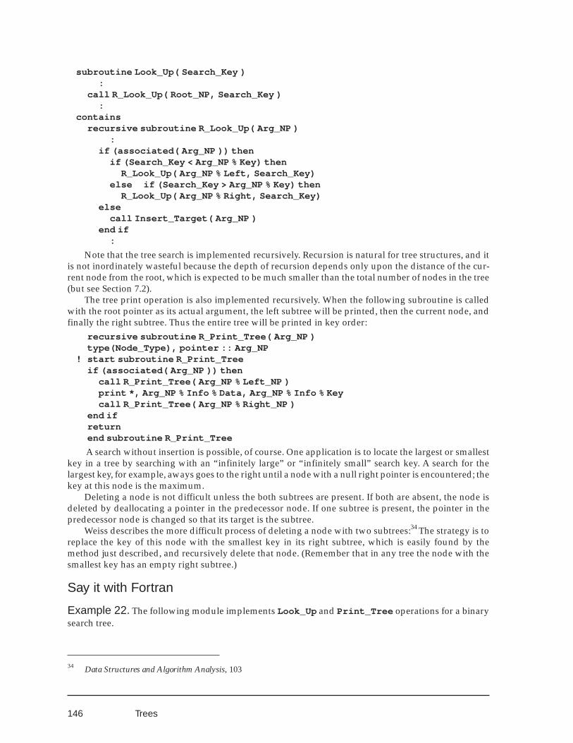
146
subroutine Look_Up( Search_Key ):
call R_Look_Up( Root_NP, Search_Key ):
containsrecursive subroutine R_Look_Up( Arg_NP )
:if (associated( Arg_NP )) then
if (Search_Key < Arg_NP % Key) thenR_Look_Up( Arg_NP % Left, Search_Key)
else if (Search_Key > Arg_NP % Key) thenR_Look_Up( Arg_NP % Right, Search_Key)
elsecall Insert_Target( Arg_NP )
end if:
Note that the tree search is implemented recursively. Recursion is natural for tree structures, and itis not inordinately wasteful because the depth of recursion depends only upon the distance of the cur-rent node from the root, which is expected to be much smaller than the total number of nodes in the tree(but see Section 7.2).
The tree print operation is also implemented recursively. When the following subroutine is calledwith the root pointer as its actual argument, the left subtree will be printed, then the current node, andfinally the right subtree. Thus the entire tree will be printed in key order:
recursive subroutine R_Print_Tree( Arg_NP )type(Node_Type), pointer :: Arg_NP
! start subroutine R_Print_Treeif (associated( Arg_NP )) then
call R_Print_Tree( Arg_NP % Left_NP )print *, Arg_NP % Info % Data, Arg_NP % Info % Keycall R_Print_Tree( Arg_NP % Right_NP )
end ifreturnend subroutine R_Print_Tree
A search without insertion is possible, of course. One application is to locate the largest or smallestkey in a tree by searching with an “infinitely large” or “infinitely small” search key. A search for thelargest key, for example, aways goes to the right until a node with a null right pointer is encountered; thekey at this node is the maximum.
Deleting a node is not difficult unless the both subtrees are present. If both are absent, the node isdeleted by deallocating a pointer in the predecessor node. If one subtree is present, the pointer in thepredecessor node is changed so that its target is the subtree.
Weiss describes the more difficult process of deleting a node with two subtrees:34 The strategy is toreplace the key of this node with the smallest key in its right subtree, which is easily found by themethod just described, and recursively delete that node. (Remember that in any tree the node with thesmallest key has an empty right subtree.)
Say it with Fortran
Example 22. The following module implements Look_Up and Print_Tree operations for a binarysearch tree.
Trees
34 Data Structures and Algorithm Analysis, 103
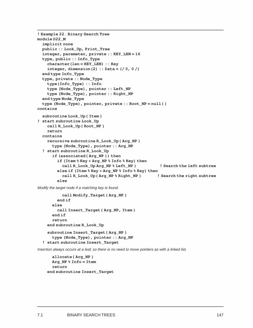
147
! Example 22. Binary Search Treemodule D22_M
implicit nonepublic :: Look_Up, Print_Treeinteger, parameter, private :: KEY_LEN = 16type, public :: Info_Type
character(len = KEY_LEN) :: Keyinteger, dimension(2) :: Data = (/ 0, 0 /)
end type Info_Typetype, private :: Node_Type
type(Info_Type) :: Infotype (Node_Type), pointer :: Left_NPtype (Node_Type), pointer :: Right_NP
end type Node_Typetype (Node_Type), pointer, private :: Root_NP = null( )
contains
subroutine Look_Up( Item )! start subroutine Look_Up
call R_Look_Up( Root_NP )return
containsrecursive subroutine R_Look_Up( Arg_NP )
type (Node_Type), pointer :: Arg_NP! start subroutine R_Look_Up
if (associated( Arg_NP )) thenif (Item % Key < Arg_NP % Info % Key) then
call R_Look_Up Arg_NP % Left_NP ) ! Search the left subtreeelse if (Item % Key > Arg_NP % Info % Key) then
call R_Look_Up( Arg_NP % Right_NP ) ! Search the right subtreeelse
Modify the target node if a matching key is found.
call Modify_Target( Arg_NP )end if
elsecall Insert_Target( Arg_NP, Item )
end ifreturn
end subroutine R_Look_Up
subroutine Insert_Target( Arg_NP )type (Node_Type), pointer :: Arg_NP
! start subroutine Insert_Target
Insertion always occurs at a leaf, so there is no need to move pointers as with a linked list.
allocate( Arg_NP )Arg_NP % Info = Itemreturn
end subroutine Insert_Target
7.1 BINARY SEARCH TREES
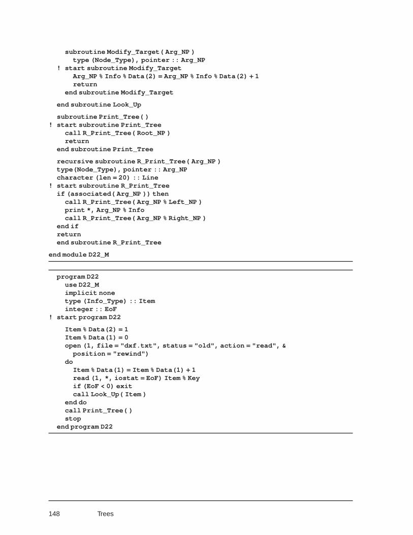
148
subroutine Modify_Target( Arg_NP )type (Node_Type), pointer :: Arg_NP
! start subroutine Modify_TargetArg_NP % Info % Data(2) = Arg_NP % Info % Data(2) + 1return
end subroutine Modify_Target
end subroutine Look_Up
subroutine Print_Tree( )! start subroutine Print_Tree
call R_Print_Tree( Root_NP )return
end subroutine Print_Tree
recursive subroutine R_Print_Tree( Arg_NP )type(Node_Type), pointer :: Arg_NPcharacter (len = 20) :: Line
! start subroutine R_Print_Treeif (associated( Arg_NP )) then
call R_Print_Tree( Arg_NP % Left_NP )print *, Arg_NP % Infocall R_Print_Tree( Arg_NP % Right_NP )
end ifreturnend subroutine R_Print_Tree
end module D22_M
program D22use D22_Mimplicit nonetype (Info_Type) :: Iteminteger :: EoF
! start program D22
Item % Data(2) = 1Item % Data(1) = 0open (1, file = "dxf.txt", status = "old", action = "read", &
position = "rewind")do
Item % Data(1) = Item % Data(1) + 1read (1, *, iostat = EoF) Item % Keyif (EoF < 0) exitcall Look_Up( Item )
end docall Print_Tree( )stop
end program D22
Trees
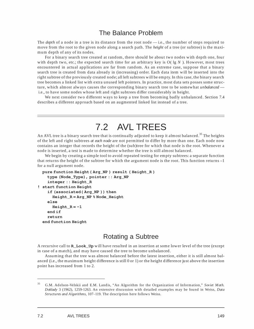
149
The Balance ProblemThe depth of a node in a tree is its distance from the root node — i.e., the number of steps required tomove from the root to the given node along a search path. The height of a tree (or subtree) is the maxi-mum depth of any of its nodes.
For a binary search tree created at random, there should be about two nodes with depth one, fourwith depth two, etc.; the expected search time for an arbitrary key is O( lg N ). However, most treesencountered in actual applications are far from random. As an extreme case, suppose that a binarysearch tree is created from data already in (increasing) order. Each data item will be inserted into theright subtree of the previously created node; all left subtrees will be empty. In this case, the binary searchtree becomes a linked list with extra unused left pointers. In practice, most data sets posses some struc-ture, which almost always causes the corresponding binary search tree to be somewhat unbalanced —i.e., to have some nodes whose left and right subtrees differ considerably in height.
We next consider two different ways to keep a tree from becoming badly unbalanced. Section 7.4describes a different approach based on an augmented linked list instead of a tree.
7.2 AVL TREESAn AVL tree is a binary search tree that is continually adjusted to keep it almost balanced.35 The heightsof the left and right subtrees at each node are not permitted to differ by more than one. Each node nowcontains an integer that records the height of the (sub)tree for which that node is the root. Whenever anode is inserted, a test is made to determine whether the tree is still almost balanced.
We begin by creating a simple tool to avoid repeated testing for empty subtrees: a separate functionthat returns the height of the subtree for which the argument node is the root. This function returns –1for a null argument node.
pure function Height( Arg_NP ) result ( Height_R )type (Node_Type), pointer :: Arg_NPinteger :: Height_R
! start function Heightif (associated( Arg_NP )) then
Height_R = Arg_NP % Node_Heightelse
Height_R = -1end ifreturn
end function Height
Rotating a SubtreeA recursive call to R_Look_Up will have resulted in an insertion at some lower level of the tree (exceptin case of a match), and may have caused the tree to become unbalanced.
Assuming that the tree was almost balanced before the latest insertion, either it is still almost bal-anced (i.e., the maximum height difference is still 0 or 1) or the height difference just above the insertionpoint has increased from 1 to 2.
7.2 AVL TREES
35 G.M. Adelson-Velskii and E.M. Landis, “An Algorithm for the Organization of Information,” Soviet Math.Doklady 3 (1962), 1259-1263. An extensive discussion with detailed examples may be found in Weiss, DataStructures and Algorithms, 107–119. The description here follows Weiss.
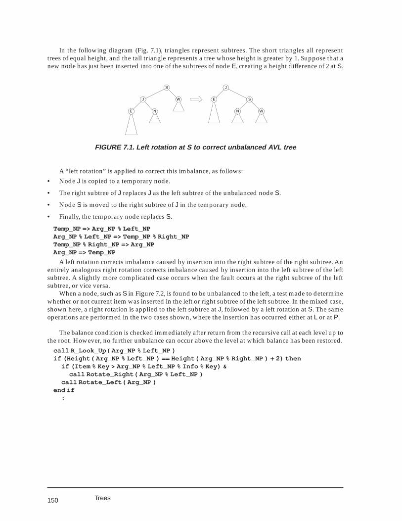
150
In the following diagram (Fig. 7.1), triangles represent subtrees. The short triangles all representtrees of equal height, and the tall triangle represents a tree whose height is greater by 1. Suppose that anew node has just been inserted into one of the subtrees of node E, creating a height difference of 2 at S.
J
N
E
E
J
S
W S
N W
FIGURE 7.1. Left rotation at S to correct unbalanced AVL tree
A “left rotation” is applied to correct this imbalance, as follows:• Node J is copied to a temporary node.
• The right subtree of J replaces J as the left subtree of the unbalanced node S.
• Node S is moved to the right subtree of J in the temporary node.
• Finally, the temporary node replaces S.
Temp_NP => Arg_NP % Left_NPArg_NP % Left_NP => Temp_NP % Right_NPTemp_NP % Right_NP => Arg_NPArg_NP => Temp_NP
A left rotation corrects imbalance caused by insertion into the right subtree of the right subtree. Anentirely analogous right rotation corrects imbalance caused by insertion into the left subtree of the leftsubtree. A slightly more complicated case occurs when the fault occurs at the right subtree of the leftsubtree, or vice versa.
When a node, such as S in Figure 7.2, is found to be unbalanced to the left, a test made to determinewhether or not current item was inserted in the left or right subtree of the left subtree. In the mixed case,shown here, a right rotation is applied to the left subtree at J, followed by a left rotation at S. The sameoperations are performed in the two cases shown, where the insertion has occurred either at L or at P.
Trees
The balance condition is checked immediately after return from the recursive call at each level up tothe root. However, no further unbalance can occur above the level at which balance has been restored.
call R_Look_Up( Arg_NP % Left_NP )if (Height( Arg_NP % Left_NP ) == Height( Arg_NP % Right_NP ) + 2) then
if (Item % Key > Arg_NP % Left_NP % Info % Key) &call Rotate_Right( Arg_NP % Left_NP )
call Rotate_Left( Arg_NP )end if
:
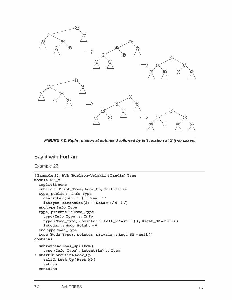
151
FIGURE 7.2. Right rotation at subtree J followed by left rotation at S (two cases)
Say it with Fortran
Example 23
! Example 23. AVL (Adelson-Velskii & Landis) Treemodule D23_M
implicit nonepublic :: Print_Tree, Look_Up, Initializetype, public :: Info_Type
character(len = 15) :: Key = " "integer, dimension(2) :: Data = (/ 0, 1 /)
end type Info_Typetype, private :: Node_Type
type(Info_Type) :: Infotype (Node_Type), pointer :: Left_NP = null( ), Right_NP = null( )integer :: Node_Height = 0
end type Node_Typetype (Node_Type), pointer, private :: Root_NP = null( )
contains
subroutine Look_Up( Item )type (Info_Type), intent(in) :: Item
! start subroutine Look_Upcall R_Look_Up( Root_NP )return
contains
J
E
L
N
P
W
S
J
E L
N
P
S
W
J
E L
N
P
S
W
J
E
L
N
P
W
S
J
E L
N
P
S
W
J
E L
N
P
S
W
7.2 AVL TREES
152
recursive subroutine R_Look_Up( Arg_NP )type (Node_Type), pointer :: Arg_NP
! start subroutine R_Look_Upif (associated( Arg_NP )) then
if (Item % Key < Arg_NP % Info % Key) thencall R_Look_Up( Arg_NP % Left_NP )
Check whether the tree is still in balance.
if (Height( Arg_NP % Left_NP ) &== Height( Arg_NP % Right_NP ) + 2) then
if (Item % Key > Arg_NP % Left_NP % Info % Key) &call Rotate_Right( Arg_NP % Left_NP )
call Rotate_Left( Arg_NP )else
Arg_NP % Node_Height = 1 + max( Height( Arg_NP % Left_NP ), &Height( Arg_NP % Right_NP ) )
end ifelse if (Item % Key > Arg_NP % Info % Key) then
Same as the previous case, except that Right and Left are interchanged.
:else ! Item % Key == Arg_NP % Info % Key
call Modify_Target( Arg_NP )end if
elsecall Insert_Target( Arg_NP )
end ifreturn
contains
subroutine Rotate_Left( Arg_NP )type (Node_Type), pointer :: Arg_NPtype (Node_Type), pointer :: Temp_NP
! start subroutine Rotate_LeftTemp_NP => Arg_NP % Left_NPArg_NP % Left_NP => Temp_NP % Right_NPTemp_NP % Right_NP => Arg_NPArg_NP % Node_Height = 1 + &
max( Height( Arg_NP % Left_NP ), Height( Arg_NP % Right_NP ) )Temp_NP % Node_Height = 1 + &
max( Height( Temp_NP % Left_NP ), Arg_NP % Node_Height )Arg_NP => Temp_NPreturn
end subroutine Rotate_Left
subroutine Rotate_Right( Arg_NP ):
end subroutine Rotate_Right
pure function Height( Arg_NP ) result ( Height_R ):
end function Height
Subroutines Modify_Target , Insert_Target , and Print_Tree go here
end subroutine Look_Up
end module D23_M
Trees
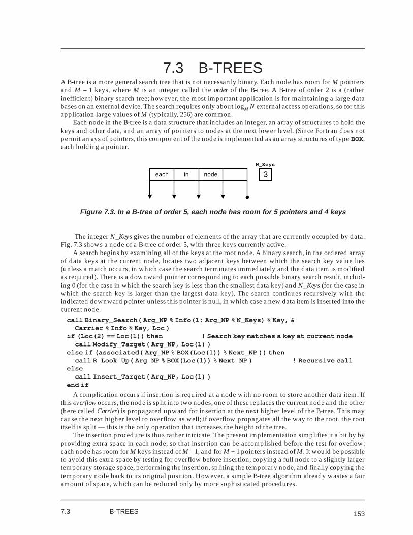
153
7.3 B-TREESA B-tree is a more general search tree that is not necessarily binary. Each node has room for M pointersand M – 1 keys, where M is an integer called the order of the B-tree. A B-tree of order 2 is a (ratherinefficient) binary search tree; however, the most important application is for maintaining a large databases on an external device. The search requires only about logM N external access operations, so for thisapplication large values of M (typically, 256) are common.
Each node in the B-tree is a data structure that includes an integer, an array of structures to hold thekeys and other data, and an array of pointers to nodes at the next lower level. (Since Fortran does notpermit arrays of pointers, this component of the node is implemented as an array structures of type BOX,each holding a pointer.
7.3 B-TREES
each in node 3N_Keys
Figure 7.3. In a B-tree of order 5, each node has room for 5 pointers and 4 keys
The integer N_Keys gives the number of elements of the array that are currently occupied by data.Fig. 7.3 shows a node of a B-tree of order 5, with three keys currently active.
A search begins by examining all of the keys at the root node. A binary search, in the ordered arrayof data keys at the current node, locates two adjacent keys between which the search key value lies(unless a match occurs, in which case the search terminates immediately and the data item is modifiedas required). There is a downward pointer corresponding to each possible binary search result, includ-ing 0 (for the case in which the search key is less than the smallest data key) and N_Keys (for the case inwhich the search key is larger than the largest data key). The search continues recursively with theindicated downward pointer unless this pointer is null, in which case a new data item is inserted into thecurrent node.
call Binary_Search( Arg_NP % Info(1: Arg_NP % N_Keys) % Key, &Carrier % Info % Key, Loc )
if (Loc(2) == Loc(1)) then ! Search key matches a key at current nodecall Modify_Target( Arg_NP, Loc(1) )
else if (associated( Arg_NP % BOX(Loc(1)) % Next_NP )) thencall R_Look_Up( Arg_NP % BOX(Loc(1)) % Next_NP ) ! Recursive call
elsecall Insert_Target( Arg_NP, Loc(1) )
end if
A complication occurs if insertion is required at a node with no room to store another data item. Ifthis overflow occurs, the node is split into two nodes; one of these replaces the current node and the other(here called Carrier) is propagated upward for insertion at the next higher level of the B-tree. This maycause the next higher level to overflow as well; if overflow propagates all the way to the root, the rootitself is split — this is the only operation that increases the height of the tree.
The insertion procedure is thus rather intricate. The present implementation simplifies it a bit by byproviding extra space in each node, so that insertion can be accomplished before the test for oveflow:each node has room for M keys instead of M – 1, and for M + 1 pointers instead of M. It would be possibleto avoid this extra space by testing for overflow before insertion, copying a full node to a slightly largertemporary storage space, performing the insertion, spliting the temporary node, and finally copying thetemporary node back to its original position. However, a simple B-tree algorithm already wastes a fairamount of space, which can be reduced only by more sophisticated procedures.
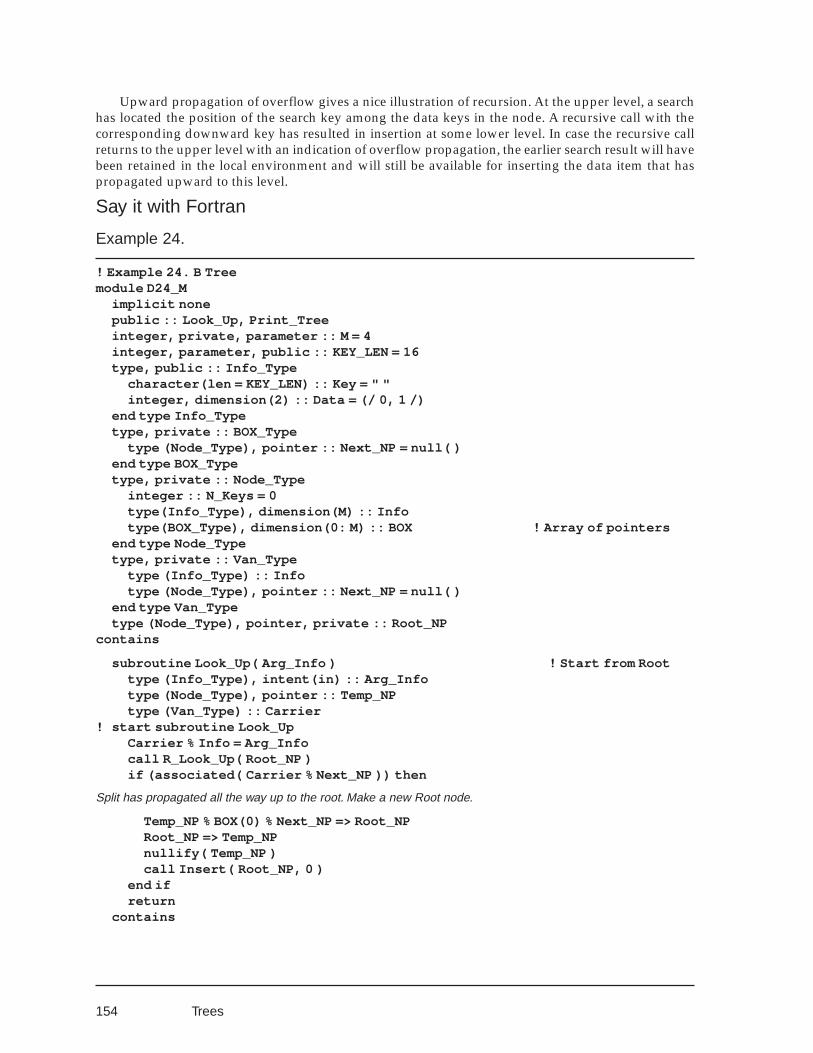
154
Upward propagation of overflow gives a nice illustration of recursion. At the upper level, a searchhas located the position of the search key among the data keys in the node. A recursive call with thecorresponding downward key has resulted in insertion at some lower level. In case the recursive callreturns to the upper level with an indication of overflow propagation, the earlier search result will havebeen retained in the local environment and will still be available for inserting the data item that haspropagated upward to this level.
Say it with Fortran
Example 24.
! Example 24. B Treemodule D24_M
implicit nonepublic :: Look_Up, Print_Treeinteger, private, parameter :: M = 4integer, parameter, public :: KEY_LEN = 16type, public :: Info_Type
character(len = KEY_LEN) :: Key = " "integer, dimension(2) :: Data = (/ 0, 1 /)
end type Info_Typetype, private :: BOX_Type
type (Node_Type), pointer :: Next_NP = null( )end type BOX_Typetype, private :: Node_Type
integer :: N_Keys = 0type(Info_Type), dimension(M) :: Infotype(BOX_Type), dimension(0: M) :: BOX ! Array of pointers
end type Node_Typetype, private :: Van_Type
type (Info_Type) :: Infotype (Node_Type), pointer :: Next_NP = null( )
end type Van_Typetype (Node_Type), pointer, private :: Root_NP
contains
subroutine Look_Up( Arg_Info ) ! Start from Roottype (Info_Type), intent(in) :: Arg_Infotype (Node_Type), pointer :: Temp_NPtype (Van_Type) :: Carrier
! start subroutine Look_UpCarrier % Info = Arg_Infocall R_Look_Up( Root_NP )if (associated( Carrier % Next_NP )) then
Split has propagated all the way up to the root. Make a new Root node.
Temp_NP % BOX(0) % Next_NP => Root_NPRoot_NP => Temp_NPnullify( Temp_NP )call Insert( Root_NP, 0 )
end ifreturn
contains
Trees
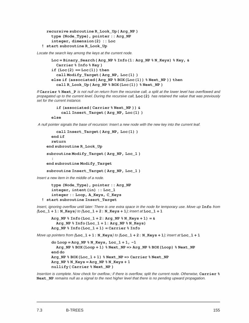
155
recursive subroutine R_Look_Up( Arg_NP )type (Node_Type), pointer :: Arg_NPinteger, dimension(2) :: Loc
! start subroutine R_Look_Up
Locate the search key among the keys at the current node.
Loc = Binary_Search( Arg_NP % Info(1: Arg_NP % N_Keys) % Key, &Carrier % Info % Key )
if (Loc(2) == Loc(1)) thencall Modify_Target( Arg_NP, Loc(1) )
else if (associated( Arg_NP % BOX(Loc(1)) % Next_NP )) thencall R_Look_Up( Arg_NP % BOX(Loc(1)) % Next_NP )
If Carrier % Next_P is not null on return from the recursive call, a split at the lower level has overflowed andpropagated up to the current level. During the recursive call, Loc(2) has retained the value that was previouslyset for the current instance.
if (associated( Carrier % Next_NP )) &call Insert_Target( Arg_NP, Loc(1) )
else
A null pointer signals the base of recursion: Insert a new node with the new key into the current leaf.
call Insert_Target( Arg_NP, Loc(1) )end ifreturn
end subroutine R_Look_Up
subroutine Modify_Target( Arg_NP, Loc_1 ):
end subroutine Modify_Target
subroutine Insert_Target( Arg_NP, Loc_1 )
Insert a new item in the middle of a node.
type (Node_Type), pointer :: Arg_NPinteger, intent(in) :: Loc_1integer :: Loop, A_Keys, C_Keys
! start subroutine Insert_Target
Insert, ignoring overflow until later: There is one extra space in the node for temporary use. Move up Info from{Loc_1 + 1: N_Keys } to {Loc_1 + 2: N_Keys + 1}; insert at Loc_1 + 1
Arg_NP % Info(Loc_1 + 2: Arg_NP % N_Keys + 1) = &Arg_NP % Info(Loc_1 + 1: Arg_NP % N_Keys)
Arg_NP % Info(Loc_1 + 1) = Carrier % Info
Move up pointers from {Loc_1 + 1: N_Keys } to {Loc_1 + 2: N_Keys + 1}; insert at Loc_1 + 1
do Loop = Arg_NP % N_Keys, Loc_1 + 1, -1Arg_NP % BOX(Loop + 1) % Next_NP => Arg_NP % BOX(Loop) % Next_NP
end doArg_NP % BOX(Loc_1 + 1) % Next_NP => Carrier % Next_NPArg_NP % N_Keys = Arg_NP % N_Keys + 1nullify( Carrier % Next_NP )
Insertion is complete. Now check for oveflow.; if there is overflow, split the current node. Otherwise, Carrier %Next_NP remains null as a signal to the next higher level that there is no pending upward propagation.
7.3 B-TREES
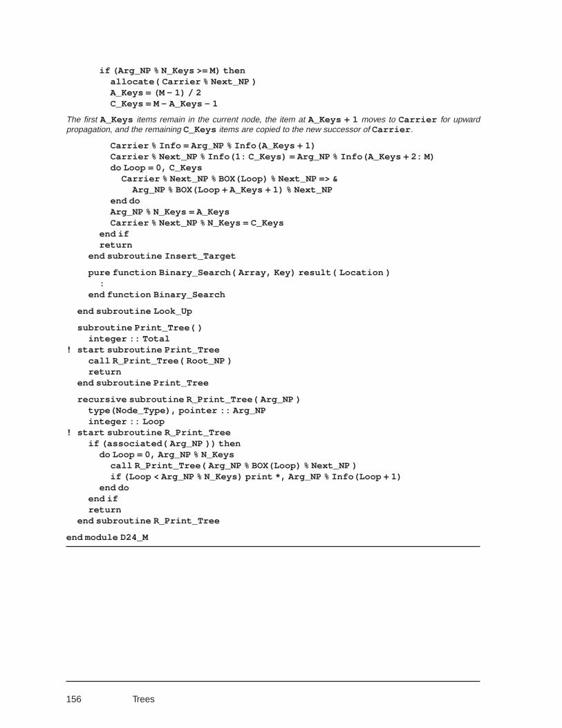
156
if (Arg_NP % N_Keys >= M) thenallocate( Carrier % Next_NP )A_Keys = (M - 1) / 2C_Keys = M - A_Keys - 1
The first A_Keys items remain in the current node, the item at A_Keys + 1 moves to Carrier for upwardpropagation, and the remaining C_Keys items are copied to the new successor of Carrier .
Carrier % Info = Arg_NP % Info(A_Keys + 1)Carrier % Next_NP % Info(1: C_Keys) = Arg_NP % Info(A_Keys + 2: M)do Loop = 0, C_Keys
Carrier % Next_NP % BOX(Loop) % Next_NP => &Arg_NP % BOX(Loop + A_Keys + 1) % Next_NP
end doArg_NP % N_Keys = A_KeysCarrier % Next_NP % N_Keys = C_Keys
end ifreturn
end subroutine Insert_Target
pure function Binary_Search( Array, Key) result( Location ):
end function Binary_Search
end subroutine Look_Up
subroutine Print_Tree( )integer :: Total
! start subroutine Print_Treecall R_Print_Tree( Root_NP )return
end subroutine Print_Tree
recursive subroutine R_Print_Tree( Arg_NP )type(Node_Type), pointer :: Arg_NPinteger :: Loop
! start subroutine R_Print_Treeif (associated( Arg_NP )) then
do Loop = 0, Arg_NP % N_Keyscall R_Print_Tree( Arg_NP % BOX(Loop) % Next_NP )if (Loop < Arg_NP % N_Keys) print *, Arg_NP % Info(Loop + 1)
end doend ifreturn
end subroutine R_Print_Tree
end module D24_M
Trees
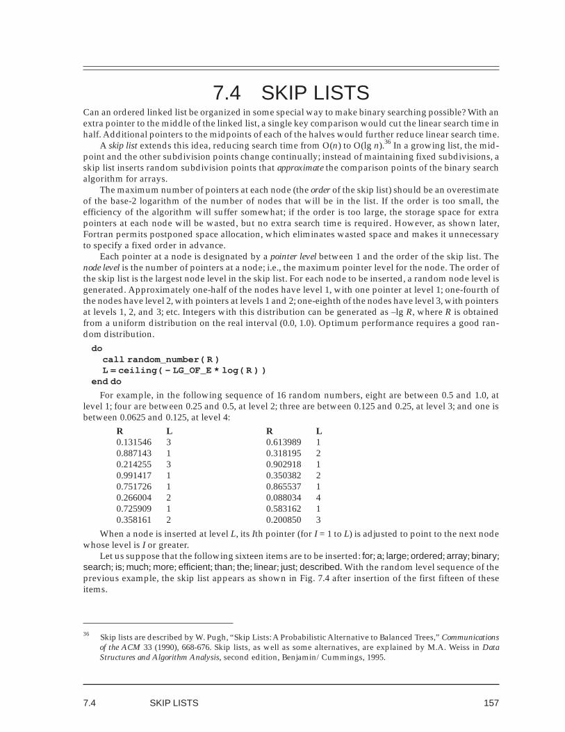
157
7.4 SKIP LISTSCan an ordered linked list be organized in some special way to make binary searching possible? With anextra pointer to the middle of the linked list, a single key comparison would cut the linear search time inhalf. Additional pointers to the midpoints of each of the halves would further reduce linear search time.
A skip list extends this idea, reducing search time from O(n) to O(lg n).36 In a growing list, the mid-point and the other subdivision points change continually; instead of maintaining fixed subdivisions, askip list inserts random subdivision points that approximate the comparison points of the binary searchalgorithm for arrays.
The maximum number of pointers at each node (the order of the skip list) should be an overestimateof the base-2 logarithm of the number of nodes that will be in the list. If the order is too small, theefficiency of the algorithm will suffer somewhat; if the order is too large, the storage space for extrapointers at each node will be wasted, but no extra search time is required. However, as shown later,Fortran permits postponed space allocation, which eliminates wasted space and makes it unnecessaryto specify a fixed order in advance.
Each pointer at a node is designated by a pointer level between 1 and the order of the skip list. Thenode level is the number of pointers at a node; i.e., the maximum pointer level for the node. The order ofthe skip list is the largest node level in the skip list. For each node to be inserted, a random node level isgenerated. Approximately one-half of the nodes have level 1, with one pointer at level 1; one-fourth ofthe nodes have level 2, with pointers at levels 1 and 2; one-eighth of the nodes have level 3, with pointersat levels 1, 2, and 3; etc. Integers with this distribution can be generated as –lg R, where R is obtainedfrom a uniform distribution on the real interval (0.0, 1.0). Optimum performance requires a good ran-dom distribution.
docall random_number( R )L = ceiling( - LG_OF_E * log( R ) )
end do
For example, in the following sequence of 16 random numbers, eight are between 0.5 and 1.0, atlevel 1; four are between 0.25 and 0.5, at level 2; three are between 0.125 and 0.25, at level 3; and one isbetween 0.0625 and 0.125, at level 4:
R L R L0.131546 3 0.613989 10.887143 1 0.318195 20.214255 3 0.902918 10.991417 1 0.350382 20.751726 1 0.865537 10.266004 2 0.088034 40.725909 1 0.583162 10.358161 2 0.200850 3
When a node is inserted at level L, its Ith pointer (for I = 1 to L) is adjusted to point to the next nodewhose level is I or greater.
Let us suppose that the following sixteen items are to be inserted: for; a; large; ordered; array; binary;search; is; much; more; efficient; than; the; linear; just; described. With the random level sequence of theprevious example, the skip list appears as shown in Fig. 7.4 after insertion of the first fifteen of theseitems.
7.4 SKIP LISTS
36 Skip lists are described by W. Pugh, “Skip Lists: A Probabilistic Alternative to Balanced Trees,” Communicationsof the ACM 33 (1990), 668-676. Skip lists, as well as some alternatives, are explained by M.A. Weiss in DataStructures and Algorithm Analysis, second edition, Benjamin/Cummings, 1995.
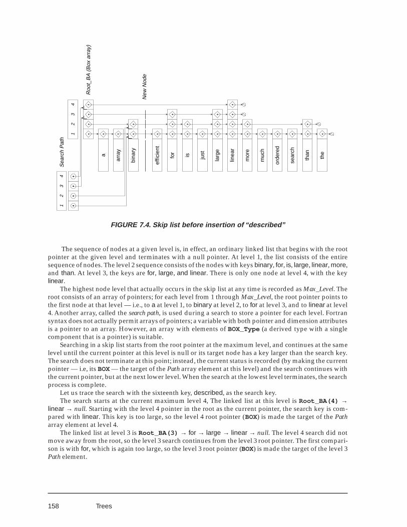
158
Roo
t_B
A (
Box
arr
ay)
a
arra
y
bina
ry
effic
ient
for
is just
larg
e
linea
r
mor
e
muc
h
orde
red
sear
ch
than the
Sea
rch
Pat
h
New
Nod
e
12
34
12
34
FIGURE 7.4. Skip list before insertion of “described”
The sequence of nodes at a given level is, in effect, an ordinary linked list that begins with the rootpointer at the given level and terminates with a null pointer. At level 1, the list consists of the entiresequence of nodes. The level 2 sequence consists of the nodes with keys binary, for, is, large, linear, more,and than. At level 3, the keys are for, large, and linear. There is only one node at level 4, with the keylinear.
The highest node level that actually occurs in the skip list at any time is recorded as Max_Level. Theroot consists of an array of pointers; for each level from 1 through Max_Level, the root pointer points tothe first node at that level — i.e., to a at level 1, to binary at level 2, to for at level 3, and to linear at level4. Another array, called the search path, is used during a search to store a pointer for each level. Fortransyntax does not actually permit arrays of pointers; a variable with both pointer and dimension attributesis a pointer to an array. However, an array with elements of BOX_Type (a derived type with a singlecomponent that is a pointer) is suitable.
Searching in a skip list starts from the root pointer at the maximum level, and continues at the samelevel until the current pointer at this level is null or its target node has a key larger than the search key.The search does not terminate at this point; instead, the current status is recorded (by making the currentpointer — i.e, its BOX— the target of the Path array element at this level) and the search continues withthe current pointer, but at the next lower level. When the search at the lowest level terminates, the searchprocess is complete.
Let us trace the search with the sixteenth key, described, as the search key.The search starts at the current maximum level 4, The linked list at this level is Root_BA(4) →
linear → null. Starting with the level 4 pointer in the root as the current pointer, the search key is com-pared with linear. This key is too large, so the level 4 root pointer (BOX) is made the target of the Patharray element at level 4.
The linked list at level 3 is Root_BA(3) → for → large → linear → null. The level 4 search did notmove away from the root, so the level 3 search continues from the level 3 root pointer. The first compari-son is with for, which is again too large, so the level 3 root pointer (BOX) is made the target of the level 3Path element.
Trees
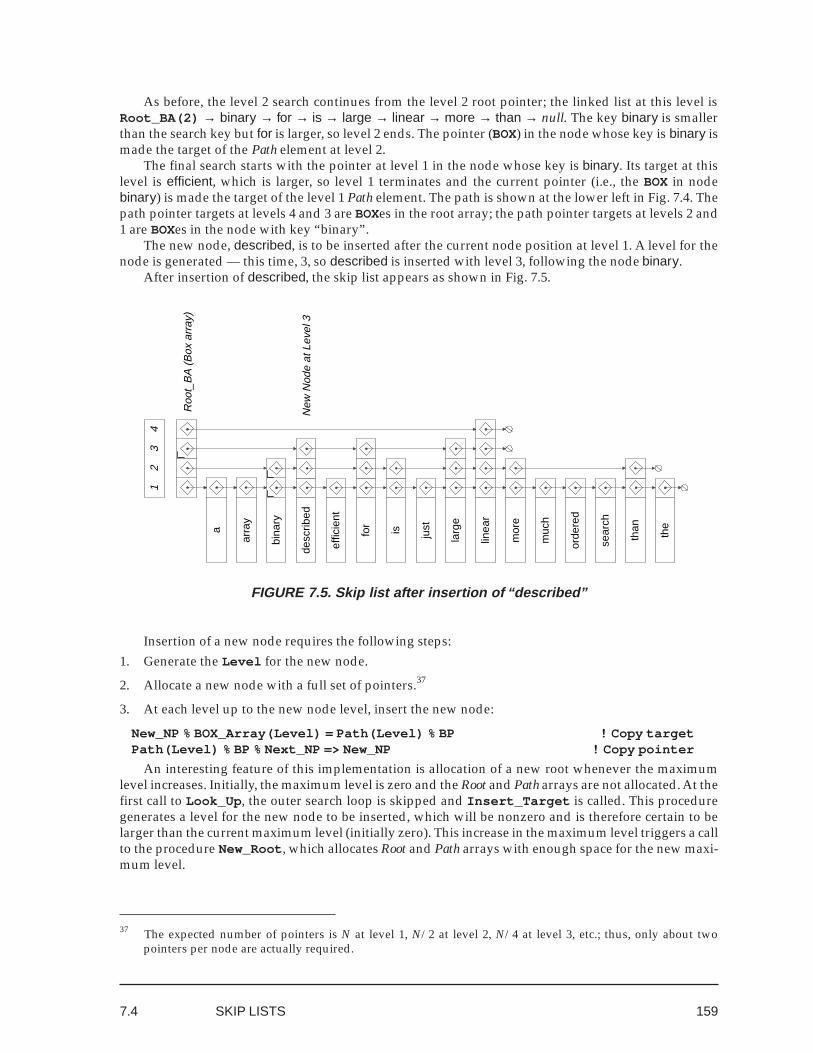
159
As before, the level 2 search continues from the level 2 root pointer; the linked list at this level isRoot_BA(2) → binary → for → is → large → linear → more → than → null. The key binary is smallerthan the search key but for is larger, so level 2 ends. The pointer (BOX) in the node whose key is binary ismade the target of the Path element at level 2.
The final search starts with the pointer at level 1 in the node whose key is binary. Its target at thislevel is efficient, which is larger, so level 1 terminates and the current pointer (i.e., the BOX in nodebinary) is made the target of the level 1 Path element. The path is shown at the lower left in Fig. 7.4. Thepath pointer targets at levels 4 and 3 are BOXes in the root array; the path pointer targets at levels 2 and1 are BOXes in the node with key “binary”.
The new node, described, is to be inserted after the current node position at level 1. A level for thenode is generated — this time, 3, so described is inserted with level 3, following the node binary.
After insertion of described, the skip list appears as shown in Fig. 7.5.
a
arra
y
bina
ry
effic
ient
for
is just
larg
e
linea
r
mor
e
muc
h
orde
red
sear
ch
than the
desc
ribed
New
Nod
e at
Lev
el 3
12
34
Roo
t_B
A (
Box
arr
ay)
FIGURE 7.5. Skip list after insertion of “described”
Insertion of a new node requires the following steps:1. Generate the Level for the new node.
2. Allocate a new node with a full set of pointers.37
3. At each level up to the new node level, insert the new node:
New_NP % BOX_Array(Level) = Path(Level) % BP ! Copy targetPath(Level) % BP % Next_NP => New_NP ! Copy pointer
An interesting feature of this implementation is allocation of a new root whenever the maximumlevel increases. Initially, the maximum level is zero and the Root and Path arrays are not allocated. At thefirst call to Look_Up , the outer search loop is skipped and Insert_Target is called. This proceduregenerates a level for the new node to be inserted, which will be nonzero and is therefore certain to belarger than the current maximum level (initially zero). This increase in the maximum level triggers a callto the procedure New_Root , which allocates Root and Path arrays with enough space for the new maxi-mum level.
7.4 SKIP LISTS
37 The expected number of pointers is N at level 1, N/2 at level 2, N/4 at level 3, etc.; thus, only about twopointers per node are actually required.
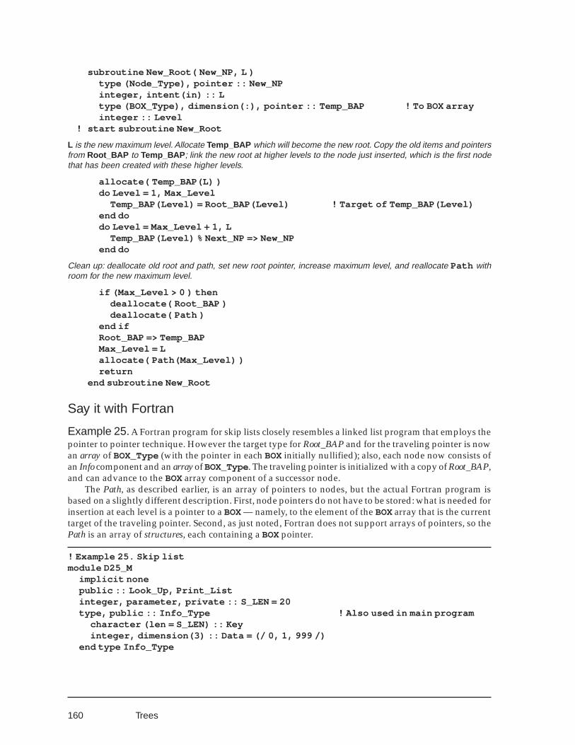
160
subroutine New_Root( New_NP, L )type (Node_Type), pointer :: New_NPinteger, intent(in) :: Ltype (BOX_Type), dimension(:), pointer :: Temp_BAP ! To BOX arrayinteger :: Level
! start subroutine New_Root
L is the new maximum level. Allocate Temp_BAP which will become the new root. Copy the old items and pointersfrom Root_BAP to Temp_BAP ; link the new root at higher levels to the node just inserted, which is the first nodethat has been created with these higher levels.
allocate( Temp_BAP(L) )do Level = 1, Max_Level
Temp_BAP(Level) = Root_BAP(Level) ! Target of Temp_BAP(Level)end dodo Level = Max_Level + 1, L
Temp_BAP(Level) % Next_NP => New_NPend do
Clean up: deallocate old root and path, set new root pointer, increase maximum level, and reallocate Path withroom for the new maximum level.
if (Max_Level > 0 ) thendeallocate( Root_BAP )deallocate( Path )
end ifRoot_BAP => Temp_BAPMax_Level = Lallocate( Path(Max_Level) )return
end subroutine New_Root
Say it with Fortran
Example 25. A Fortran program for skip lists closely resembles a linked list program that employs thepointer to pointer technique. However the target type for Root_BAP and for the traveling pointer is nowan array of BOX_Type (with the pointer in each BOX initially nullified); also, each node now consists ofan Info component and an array of BOX_Type. The traveling pointer is initialized with a copy of Root_BAP,and can advance to the BOX array component of a successor node.
The Path, as described earlier, is an array of pointers to nodes, but the actual Fortran program isbased on a slightly different description. First, node pointers do not have to be stored: what is needed forinsertion at each level is a pointer to a BOX— namely, to the element of the BOX array that is the currenttarget of the traveling pointer. Second, as just noted, Fortran does not support arrays of pointers, so thePath is an array of structures, each containing a BOX pointer.
! Example 25. Skip listmodule D25_M
implicit nonepublic :: Look_Up, Print_Listinteger, parameter, private :: S_LEN = 20type, public :: Info_Type ! Also used in main program
character (len = S_LEN) :: Keyinteger, dimension(3) :: Data = (/ 0, 1, 999 /)
end type Info_Type
Trees
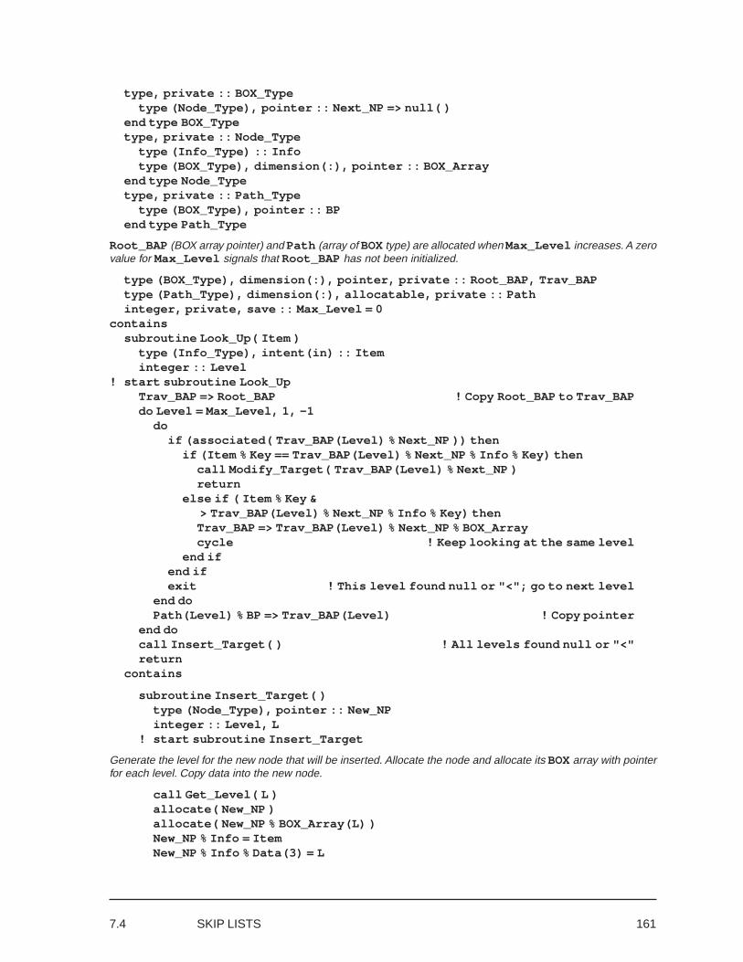
161
type, private :: BOX_Typetype (Node_Type), pointer :: Next_NP => null( )
end type BOX_Typetype, private :: Node_Type
type (Info_Type) :: Infotype (BOX_Type), dimension(:), pointer :: BOX_Array
end type Node_Typetype, private :: Path_Type
type (BOX_Type), pointer :: BPend type Path_Type
Root_BAP (BOX array pointer) and Path (array of BOX type) are allocated when Max_Level increases. A zerovalue for Max_Level signals that Root_BAP has not been initialized.
type (BOX_Type), dimension(:), pointer, private :: Root_BAP, Trav_BAPtype (Path_Type), dimension(:), allocatable, private :: Pathinteger, private, save :: Max_Level = 0
containssubroutine Look_Up( Item )
type (Info_Type), intent(in) :: Iteminteger :: Level
! start subroutine Look_UpTrav_BAP => Root_BAP ! Copy Root_BAP to Trav_BAPdo Level = Max_Level, 1, -1
doif (associated( Trav_BAP(Level) % Next_NP )) then
if (Item % Key == Trav_BAP(Level) % Next_NP % Info % Key) thencall Modify_Target( Trav_BAP(Level) % Next_NP )return
else if ( Item % Key & > Trav_BAP(Level) % Next_NP % Info % Key) thenTrav_BAP => Trav_BAP(Level) % Next_NP % BOX_Arraycycle ! Keep looking at the same level
end ifend ifexit ! This level found null or "<"; go to next level
end doPath(Level) % BP => Trav_BAP(Level) ! Copy pointer
end docall Insert_Target( ) ! All levels found null or "<"return
contains
subroutine Insert_Target( )type (Node_Type), pointer :: New_NPinteger :: Level, L
! start subroutine Insert_Target
Generate the level for the new node that will be inserted. Allocate the node and allocate its BOX array with pointerfor each level. Copy data into the new node.
call Get_Level( L )allocate( New_NP )allocate( New_NP % BOX_Array(L) )New_NP % Info = ItemNew_NP % Info % Data(3) = L
7.4 SKIP LISTS
162
Use Path to link the new node into the skip list at each level. If the level of the new node exceeds Max_Level ,a new Root_BAP will be generated and the higher levels will be linked to it.
do Level = 1, min( L, Max_Level )New_NP % BOX_Array(Level) = Path(Level) % BPPath(Level) % BP % Next_NP => New_NP
end doif (L > Max_Level) call New_Root( New_NP, L )return
end subroutine Insert_Target
subroutine Get_Level( L ):
end subroutine Get_Level
subroutine Modify_Target( Arg_NP ):
end subroutine Modify_Target
subroutine New_Root( New_NP, L ):
end subroutine New_Root
end subroutine Look_Up
subroutine Print_List( )! start subroutine Print_List
Trav_BAP => Root_BAPdo while (associated( Trav_BAP(1) % Next_NP ))
print *, Trav_BAP(1) % Next_NP % InfoTrav_BAP => Trav_BAP(1) % Next_NP % BOX_Array ! Advance to next node
end doreturn
end subroutine Print_List
end module D25_M
7.5 COMPARISON OF ALGORITHMSA sequence of 1,024 character strings, with 27 duplicates and 997 different strings, was generated ran-domly (see the electronically distributed file dxf.txt ). These were then inserted into an array, a linkedlist, a simple binary search tree, an AVL tree, B trees of order 2, 4, and 32, and a skip list. Comparisonsand other relevant operations were counted during the tests.
An array (with binary search) required 9,765 comparisons and 245,314 moves.A linked list required 261,245 comparisons.A simple binary search tree required 12,363 comparisons and reached level 20. Considerably worse
performance might be expected with nonrandom input data.An AVL tree required 9,858 comparisons and 668 rotations; the maximum level was 11.A B tree of order 2 (level 30) required 38,285 comparisons and 5,066 moves; order 4 (level 7) required
14,613 comparisons and 2,807 moves; order 32 (level 3) required 11,165 comparisons and 12,327 moves.A skip list required 14,825 comparisons; the final maximum level was 9. (This test employed the
“good” random number generator in the electronic version of the skip list module. One intrinsicrandom_number subroutine required more than 19,000 comparisons.)
Trees
163
Conclusions:
For maintaining an expanding list in internal storage, the two best choices, among the alternatives de-scribed in this book, are an AVL tree and a skip list. The AVL tree requires fewer comparisons, butrotations are rather expensive. The skip list is more complicated, but would probably be more efficientover all.
7.5 COMPARISON OF ALGORITHMS
164
POSSIBLE ANSWER to Exercise 5, Section 1.2 (page 35):
! Binary search in ordered array (with recursion).pure function Search (Array, Key) result (Location)
real, intent(in), dimension(:) :: Arrayreal, intent(in) :: Keyinteger :: Location(2)
! start function SearchLocation = Recursive_Binary_Search( 0, size(Array) + 1 )return
containspure recursive function Recursive_Binary_Search( L_1, L_2 ) &
result( L_R )integer, intent(in) :: L_1, L_2integer, dimension(2) :: L_Rinteger :: Middle
! start function Recursive_Binary_Searchif (L_2 - L_1 <= 1) then
L_R = (/ L_1, L_2 /) ! Array constructorelse
Middle = (L_1 + L_2) / 2if (Key > Array(Middle)) then
L_R = Recursive_Binary_Search( Middle, L_2 )else if (Key < Array(Middle)) then
L_R = Recursive_Binary_Search( L_1, Middle )else
L_R = Middle ! Whole array assignmentend if
end ifreturn
end function Recursive_Binary_Searchend function Search
165
Index
abstraction 121, 126–27, 134, 137activation record 79, 91, 109–10, 125algorithm 61, 64, 81–82, 89–90, 94–99, 119–21,
145–46, 149, 154, 157allocate 29–41, 57–59, 92–105, 111, 114, 130–31,
134–35, 139–42, 147, 156, 159–61array 1–35, 41, 119–20
see also input and output, ordered array,rank, section, shape, storage sequence,subscript, whole array
array constructor 10array of pointers 41array of structures 3, 47–49array section 2, 13–14, 22–34, 40, 55, 61–65association status of pointer 36–38assumed length 14, 46, 56assumed shape 5, 20–48, 56, 63asymptotic analysis 90, 97–99automatic storage 20–36
see also activation recordauxiliary variable 11, 47–49, 54, 66AVL tree 149–51, 162–63balanced tree 120, 149–52, 157
see also AVL tree, B-tree, skip listbinary insertion 60–63, 76, 95–100binary search 15–19, 34–35, 60–61, 75, 96, 119–20,
145, 154–57, 162–64binary search tree 145–49, 153, 162binary tree 64, 145BOX (structure containing a pointer) 57–58, 108,
112–118, 137–39, 153–62Brainerd 103B-tree 153bubble sorting 43character length 14
see also assumed lengthcircular buffer 141–44circular linked list 118complexity 99–100
see also algorithm; asymptotic analysisconstructor, array 10Crout 24–33cuttoff (in quicksort) 90–93
dangling pointer 39data abstraction 126
see also abstractiondeallocate 38–39deferred shape array 46dequeue 136–44dereferencing of pointer 38derived type 48, 59, 103, 126, 132–34, 158DO construct 63, 83
see also loopdoubly linked list 118dummy argument 3, 46–47, 56, 63, 109, 125, 134elimination, Gauss 20–24encapsulation 126
see also abstractionenqueue 136–44factorization, Crout 24–34Fibonacci 80–82, 101function result 19, 105, 125garbage 39Gauss 20–24go to 82–83, 161graph 121, 126Hanoi puzzle 80heap storage 37–41, 59heapsort 43, 64–66, 74–76, 96–100information hiding 126–27, 134
see also abstractioninitial value of pointer 36–41inheritance 15, 125input and output of array 9
see also arrayinsertion sort 43, 52–66, 73, 76, 80, 90–100,
104–08, 113–14, 118–20, 145–50, 153–60see also binary insertion
intent 46intrinsic function 7, 50, 95iteration 13–15, 18–19, 22–36, 45, 55, 73–74, 77–82,
93–95, 106, 112iterative refinement 28–34key for sorting or searching 12, 15–19, 35–36, 42–
44, 47–51, 57–58, 64–65, 86–88, 96, 106–09,119–20, 145–49, 153–59
Index
166
Knuth 19, 43, 50, 64, 90L’Hospital’s rule 97labyrinth 121–24, 127, 130linear algebraic equations, systems of 20–34linear search 17linked list 61, 80, 102–13, 116–20, 127, 130–34,
137–38, 145–49, 157–60local variable 49, 79, 91, 125logarithm 27, 99, 157loop 12–19, 35, 44–51, 54–58, 61–63, 81, 90, 93–95,
99, 106, 155–56, 159Maron and Lopez 21mathematical induction 93, 101matrix 4Mauchly 60median-of-3 pivot in quicksort 86–93module 46–49, 56, 91, 102, 110–12, 115–19,
126–48, 151–56, 160–62modulo intrinsic function 141–44Moret and Shapiro 90–93null pointer 36–41object 3, 63, 102, 126–27, 134–35, 138, 142operation count 11–14, 18–19, 43, 46, 54, 61–62,
73, 75–76, 92–93, 96–97, 99optimization 80, 86, 95, 144ordered array 15–19, 96, 119–20ordered list 108overflow in B-tree 153–55pivot in quicksort 86–93, 99pointer 5, 12, 57–59, 64, 102–20, 131–39, 142,
146–61postfix 124Press 21queue 136–44quicksort 43, 74, 77–79, 86–100random number 15, 43, 46, 52–55, 60–62, 66,
73–76, 89–99, 119, 149, 157, 162rank of array or array section 2, 5, 8–11recursion 35, 77–87, 90–93, 97, 108–12, 115–17,
125–26, 145–56, 164reverse 55, 61, 76–80, 90, 117, 125–26robust 95root of list or tree 64–66, 69, 73, 102–120, 130–31,
134–39, 145–62rotation in AVL tree 150running time 11save attribute 39scalar 17–19, 57, 91, 127section of array 7–11
see also arraySedgewick 62, 97selection sort 43–46, 49–51, 55, 69, 96–97, 100shape of an array 3–8Shell sort 43, 62–66, 76, 96–97, 100–01
skip list 120, 157–63sort 42
see also binary insertion, heapsort, insertionsort, quicksort, shell sort, sort_3
sort_3 43, 75, 89, 92–93space economy 95stability of sorting algorithms 51, 55, 61–62stack 91, 97, 121–36, 139static storage 36–38Stirling’s forumula 100storage management 39storage sequence of array elements 9–10
see also arraystructures 3–5, 44, 47–48, 51, 57–59, 79, 102,
121–23, 126, 145–46, 149, 143, 157, 160subscript 2, 9–11
see also array, vector subscriptsubtree 66, 145–49swap 12, 43–50, 65, 69, 63–75, 87–88, 92–95tail recursion 82target 36–41threaded list 118Thomas and Finney 97towers of Hanoi 80tree 61, 64, 73, 79, 120, 145–56, 162–63undefined association status 36vector subscript 9–11
see also arrayWeiss 145–46, 149, 157whole array 5–7
see also arraywrapper 91, 110Zahn 15
Index