Embed Size (px)
Citation preview

FORMATION OF NETWORKED MOBILE ROBOTS
By
Samitha W. Ekanayake
Submitted in fulfillment of the requirements for the degree of
DOCTOR OF PHILOSOPHY
DEAKIN UNIVERSITY
AUSTRALIA
c© Copyright by Samitha W. Ekanayake, 2009

Formation of Networked Mobile Robots
by
Samitha Wathsala Ekanayake
This thesis presents a novel approach for controlling a robotic swarm to generate a geometric pattern
described by a given contour, and a suitable communication scheme which enables the robots to commu-
nicate with each other as an all-to-all network. One of many challenges in swarm robot coordination is
to generate geometric patterns from the robots using a decentralized control approach. Such formations
have numerous applications ranging from military to medical and space to underwater. The approach uses
artificial force based controller which navigates the robots in a decentralized manner. The mathematical
analysis of the controller for stability and cohesiveness provides a criterion for selecting the weighing
parameters for the controller. Moreover, the extendability of the concept of artificial force based control
of a swarm is demonstrated in an application specific scenario. Here, a two-stage controller which satisfy
special control requirements of an airborne guided weapon system was derived.
The requirement of simultaneous and delay-free data sharing is an absolute necessity for many mission
critical robotic systems, such as map generating, search and rescue, space exploration, land mine detection
etc,. The all-to-all wireless communication algorithm presented in this thesis provides an excellent media
for sharing the mission critical information. Apart from that it also minimizes the energy consumption
in communication by effectively controlling transmission power while preserving the QoS requirements of
the communication links. Furthermore, as a secondary result, the nodal energy saving algorithm for a
single-hop wireless data collecting network was derived and experimentally verified.
The outcomes of the entire research was presented cohesively as an application case study, which
established the links in seemingly standalone research components.

To my family

Table of Contents
Table of Contents vi
Acknowledgements viii
1 Introduction 11.1 Background . . . . . . . . . . . . . . . . . . . . . . . . . . . . . . . . . . . . . . . . . . . . 11.2 Overview of the Study . . . . . . . . . . . . . . . . . . . . . . . . . . . . . . . . . . . . . . 2
1.2.1 Contributions . . . . . . . . . . . . . . . . . . . . . . . . . . . . . . . . . . . . . . . 31.2.2 Thesis Outline . . . . . . . . . . . . . . . . . . . . . . . . . . . . . . . . . . . . . . 3
2 Swarm Robots: An introduction 62.1 Related Research Topics . . . . . . . . . . . . . . . . . . . . . . . . . . . . . . . . . . . . . 8
2.1.1 Aggregation and flocking . . . . . . . . . . . . . . . . . . . . . . . . . . . . . . . . 82.1.2 Pattern formation . . . . . . . . . . . . . . . . . . . . . . . . . . . . . . . . . . . . 102.1.3 Interactions within the Swarm - Communication and Sensing . . . . . . . . . . . . 11
2.2 Coordination and control approaches in swarms . . . . . . . . . . . . . . . . . . . . . . . . 122.2.1 Potential Field Based Approaches . . . . . . . . . . . . . . . . . . . . . . . . . . . 122.2.2 Artificial Physics Based Approaches . . . . . . . . . . . . . . . . . . . . . . . . . . 142.2.3 Behavior Based Approaches . . . . . . . . . . . . . . . . . . . . . . . . . . . . . . . 152.2.4 Other Methods . . . . . . . . . . . . . . . . . . . . . . . . . . . . . . . . . . . . . . 15
2.3 Mathematical Background . . . . . . . . . . . . . . . . . . . . . . . . . . . . . . . . . . . . 162.3.1 Lyapunov Stability . . . . . . . . . . . . . . . . . . . . . . . . . . . . . . . . . . . . 162.3.2 Complex Integration and Winding Number Theorem . . . . . . . . . . . . . . . . . 182.3.3 Perron-Frobenius Theorem . . . . . . . . . . . . . . . . . . . . . . . . . . . . . . . 20
2.4 Problem Statements . . . . . . . . . . . . . . . . . . . . . . . . . . . . . . . . . . . . . . . 202.4.1 Geometric Pattern Generation Problem . . . . . . . . . . . . . . . . . . . . . . . . 202.4.2 Communication problem . . . . . . . . . . . . . . . . . . . . . . . . . . . . . . . . . 22
3 Geometric Pattern Generation in a Multiple Robot System 243.1 Mathematical Model . . . . . . . . . . . . . . . . . . . . . . . . . . . . . . . . . . . . . . . 24
3.1.1 Shape formation algorithm . . . . . . . . . . . . . . . . . . . . . . . . . . . . . . . 253.1.2 Simulation results . . . . . . . . . . . . . . . . . . . . . . . . . . . . . . . . . . . . 27
3.2 Behavior Analysis . . . . . . . . . . . . . . . . . . . . . . . . . . . . . . . . . . . . . . . . 283.2.1 X Swarm definition . . . . . . . . . . . . . . . . . . . . . . . . . . . . . . . . . . . . 293.2.2 Cohesiveness . . . . . . . . . . . . . . . . . . . . . . . . . . . . . . . . . . . . . . . 333.2.3 Comment on stable locations inside the shape . . . . . . . . . . . . . . . . . . . . . 383.2.4 Discussion on Analysis . . . . . . . . . . . . . . . . . . . . . . . . . . . . . . . . . . 41
3.3 Summary . . . . . . . . . . . . . . . . . . . . . . . . . . . . . . . . . . . . . . . . . . . . . 42
vi

vii
4 Application Case Study: Swarming Guided Weapons 434.1 Motivation and Background . . . . . . . . . . . . . . . . . . . . . . . . . . . . . . . . . . . 434.2 Two-stage controller . . . . . . . . . . . . . . . . . . . . . . . . . . . . . . . . . . . . . . . 44
4.2.1 Horizontal Motion . . . . . . . . . . . . . . . . . . . . . . . . . . . . . . . . . . . . 454.2.2 Vertical Motion . . . . . . . . . . . . . . . . . . . . . . . . . . . . . . . . . . . . . . 474.2.3 Discussion . . . . . . . . . . . . . . . . . . . . . . . . . . . . . . . . . . . . . . . . . 48
4.3 Analysis of Release Height and Weapon Behavior . . . . . . . . . . . . . . . . . . . . . . . 484.3.1 Cohesive Stage . . . . . . . . . . . . . . . . . . . . . . . . . . . . . . . . . . . . . . 484.3.2 Release Height . . . . . . . . . . . . . . . . . . . . . . . . . . . . . . . . . . . . . . 544.3.3 Summery of the analysis . . . . . . . . . . . . . . . . . . . . . . . . . . . . . . . . . 55
4.4 Discussion on Implementation Issues . . . . . . . . . . . . . . . . . . . . . . . . . . . . . . 564.4.1 Controller Modification for Practical Implementation . . . . . . . . . . . . . . . . . 564.4.2 Implementation, Technologies and Error Models . . . . . . . . . . . . . . . . . . . 584.4.3 Obstacle Avoidance . . . . . . . . . . . . . . . . . . . . . . . . . . . . . . . . . . . 58
4.5 Simulation Results . . . . . . . . . . . . . . . . . . . . . . . . . . . . . . . . . . . . . . . . 624.5.1 Multiple Aircrafts Engaged in a Single Target . . . . . . . . . . . . . . . . . . . . . 634.5.2 Single Aircraft Engaged in Multiple Targets . . . . . . . . . . . . . . . . . . . . . . 634.5.3 Point Generated Shapes . . . . . . . . . . . . . . . . . . . . . . . . . . . . . . . . . 644.5.4 Shape Transitions . . . . . . . . . . . . . . . . . . . . . . . . . . . . . . . . . . . . 654.5.5 Addition/Removal of Agents . . . . . . . . . . . . . . . . . . . . . . . . . . . . . . 66
4.6 Summary . . . . . . . . . . . . . . . . . . . . . . . . . . . . . . . . . . . . . . . . . . . . . 67
5 Communication and Power Saving Schemes for the Swarm 695.1 Fully-Connected mesh network for effective communication . . . . . . . . . . . . . . . . . 69
5.1.1 Power Control in Wireless Networks . . . . . . . . . . . . . . . . . . . . . . . . . . 705.1.2 Problem Formulation . . . . . . . . . . . . . . . . . . . . . . . . . . . . . . . . . . 715.1.3 Iterative Controller . . . . . . . . . . . . . . . . . . . . . . . . . . . . . . . . . . . . 735.1.4 Convergence of the controller . . . . . . . . . . . . . . . . . . . . . . . . . . . . . . 74
5.2 A simple power control algorithm for mobile data collector based remote data gatheringscenario . . . . . . . . . . . . . . . . . . . . . . . . . . . . . . . . . . . . . . . . . . . . . . 775.2.1 Motivation and background . . . . . . . . . . . . . . . . . . . . . . . . . . . . . . . 775.2.2 Problem formulation . . . . . . . . . . . . . . . . . . . . . . . . . . . . . . . . . . . 775.2.3 Path loss model . . . . . . . . . . . . . . . . . . . . . . . . . . . . . . . . . . . . . . 795.2.4 Power control analysis . . . . . . . . . . . . . . . . . . . . . . . . . . . . . . . . . . 815.2.5 Experimental Results . . . . . . . . . . . . . . . . . . . . . . . . . . . . . . . . . . 83
5.3 Discussion of implementation considerations . . . . . . . . . . . . . . . . . . . . . . . . . . 865.4 Summary . . . . . . . . . . . . . . . . . . . . . . . . . . . . . . . . . . . . . . . . . . . . . 86
6 Concluding Remarks 89
Appendix I: Mathematical Function for Contour Generation 92
Bibliography 93

Acknowledgements
Pubudu Pathirana has been more than a PhD supervisor to me at my time at Deakin University, he isan excellent adviser, not only in research but in the life too, and a good friend. His guidance in the lifemakes it easy to adapt to the new lifestyle in a foreign country and his guidance in research inevitablyhelped me to understand the intricacies in research and academia. His help in producing this dissertationis invaluable.
My life in Australia could have been a havoc without the financial assistance from MarimuthuPalaniswami (Department of Electrical and Electronics Engineering, University of Melbourne), who em-ployed me as a research assistant to work on the same research project through the ARC network onsensor networks where Deakin is a partner.
I sincerely thank D.C. Bandara (Department of Production Engineering, University of Peradeniya,Sri Lanka) and Sarath Seneviratne (Department of Mechanical Engineering, University of Peradeniya, SriLanka), who encouraged and guided me to start a PhD.
Additionally there are many people in Deakin University who made my time enjoyable, I thank themall for the help and encouragement.
Above all, I am thankful to my parents, Chandradasa and Chandraleela Ekanayake, and my wifePiyumi; who dedicate their entire time for me. Also I thank our daughter Anuki for being the primereason to finish this thesis on time. This thesis is dedicated to them.
viii


Chapter 1
Introduction
“Science is a mechanism, a way of trying to improve your knowledge of nature. It is a system for testingyour thoughts against the universe, and seeing whether they match.” - Issac Asimov
Nature provides us enough design examples to “innovate”; scientists understanding the natural won-ders of the world and mimicking the natures’ designs had effectively contributed in improving the qualityof life of humans. Using natural resources to advance the life of the humans began in early days of farmingbased cultures, involving animals to perform the hard work for humans. Later people develop machineriesto replace the animal labor and mimicking animal behavior and structure: tractors replacing hardworkinganimals (horses, cows etc); aero planes, naval ships, and submarines mimicking birds, aqua birds and fishare some examples. In modern days the research in robotics open new frontiers to involve natural wondersin improving the physical wellbeing of humans.
1.1 Background
Swarm robotics, inspired by stability of the natural swarms (social insects such as ants, bees, termites,wasps, etc) that survived all the way from the beginning of life forms on earth, is an emerging areaof research among robotic researchers across the world. This thesis is an attempt to extend some newconcepts into the diverse research interests in swarm robotics. In this study, a scheme for navigation,shape formation and communication of a swarm of robots is developed enabling multitude of applications;ranging from medical to defense and space to underwater.
Although swarm or multi-agent dynamic system concept, in general, is used in several disciplines, thiswork considers the multi-agent system as a collection of loosely coupled dynamic units moving in 2 or3 dimensional space. In applications, the dynamic units can be robots, vehicles, UAVs, etc, where themotion dynamics is governed by a common control algorithm (decentralized or centralized). Multi-agentsystems have been considered in range of applications such as; agent-based systems, self-organization,distributed artificial computing, evolutionary computing. Therefore some of the results in this studycould be applied in many disciplines in multi-agent systems (other than the robotics), however we do notexplore such extensions here.
Robustness, flexibility and scalability of multi-agent dynamic systems or swarm robots make themextremely suitable, but not limited, to application domains that have to cover a large area, tasks thatare too dangerous and that need higher degree of maneuverability and dynamic scalability. This cannot be accomplished by an individual agent or a monolithic system [1]. Such applications include; datagathering from a widespread area, monitoring systems which needs dynamically assigned positions (suchas sea-bed monitoring, water quality monitoring in a lake, etc), de-mining (land mine removal) robotgroups, search and rescue support (specially in collapsed buildings) and battle field support (spying,maintaining dynamic communication links, etc).
Moreover, the characteristics of swarm based dynamic systems have been extended due to some break-through technological advances in nano-scale robots and their biological counterpart “bio-Nano robots”.
1

2 Chapter 1. Introduction
However, this technology has faced with the challenge of developing nano-scale actuators and sensor de-vices. With the advances in electronics and MEMS (Micro-Electro-Mechanical System) technology, thedevelopment of physical devices for micro-swarm robots has been making impressive progress in recentyears, indicating an opening of a wide application spectrum for swarm robotics.
As the review studies of [2, 3] suggests, main problem domains can be identified as; Coordinationand control in pattern formation, coordinated movement, obstacle avoidance, foraging, self-deploymentactivities, and communication and sensing. Although many concepts were developed for maneuveringsuch swarm of robots, there has not been a “final solution” for the multiple robot coordination problem.On the other hand, the communication within the robot group has also been investigated by manyresearchers, emerging numerous concepts varying from simple pheromone like communications to satellitebased communications. As in the control and coordination problem domain, there has not been “thesolution” for the communication problem, simply due to wide-spread application domains of the swarmrobotics.
1.2 Overview of the Study
This dissertation presents a decentralized approach for generating geometric patterns in a mobile robotgroup. Moreover, a communication scheme that facilitates the groups’ simultaneous communicationrequirements is introduced. This is crucial for effective navigation of the robots. The study is mainlyfocused on a group of robots maneuvering in an outdoor environment, however the concept can be usedfor indoor robot group equipped with carefully selected communication and sensing devices.
This study has two main aspects;
1. Developing a navigation scheme to guide a group of robots (agents) toward a target area, distributethem inside a given contour while eliminating inter-member collisions,
2. Developing a communication scheme to effectively link the robots together which enables simulta-neous communication without interferences.
Apart from the above objectives, the study presents some secondary objectives as follows:
1. Based on the above controller, derivation of a secondary navigation scheme for controlling an air-borne robotic swarm
2. Study of the control architecture in uncertainties in the sensing mechanism and modification of thenavigation scheme to deal with such uncertainties, obstacles and physical limitations of the robots.
3. Energy efficient communication scheme for remote data collection from a already deployed static/mobilewireless sensor network.
In achieving the above objectives, the following factors are considered;
• Decentralized Behavior - The swarm operates in a decentralized manner such that it does notdepend on external resources or commands. Here, communication with-in the group cannot beavoided in achieving a complex objective. However, the communication with-in the group mustexhibit characteristics that enable achieving independent operation of individuals.
• Simple Architecture - This denotes the sensing capabilities and system level functioning of individualunits. However the degree of simplicity depends on the application and size of the robot. Forexample, disposable robots can be equipped with a low cost and relatively simple architecturewhereas for mission critical robots (such as space exploration) more complex system architecturecan be employed.
• Scalability- i.e. the formation and navigation does not depend on the number of members; entailthe reconfiguration of the positions relative to each other. However, this has limitations (both lower

Chapter 1. Introduction 3
and upper bounds for the swarm size) in real-life scenario; coverage/ working radius of individualmembers determines the lower bound and the physical size and maneuvering radius determine theupper bound. Furthermore, the number of members is determined by the limitations in communi-cation too. The bandwidth and the speed of communication always have a trade-off between thesize of the network (number of nodes).
• Flexibility - i.e. the ability to adapt to new situations such as sudden change in shape, moving shapesetc which changes the stable conditions of the swarm. Like the previous case, this is also boundedby several factors; among them physical motion limitations (speed, power, etc.), communicationlimitations and localization-sensing limitations are significant.
• Robustness - The ability of the swarm to withstand undesirable changes in the environment (ob-stacles, communication failures etc.) and in the members (i.e. number of units, break-downs, etc)while achieving the underlying objective.
1.2.1 Contributions
The contribution of this work is two-fold.
A novel shape formation algorithm
In the shape formation algorithm [4, 5, 6, 7], the members in the swarm are populated inside a givencontour rather than arranging the members on the perimeter. The proposed scheme is decentralized suchthat it navigate to generate the objective formation without central coordination, either in the form of abase station or virtual leader. Moreover, the proposed architecture does not pre-determine the positionsof the members inside the shape, thus the system is stable against changes in the swarm size and theshape of the contour as well as the changes in the environments such as obstacles.
A novel concept of a fully-connected mesh network for robot communication
This mesh network enables all the members in the network to communicate with each other, using abroadcast type fully-connected mesh network [8, 9]. Moreover, the study provides an upper bound in thecapacity of the network in terms of the number of wireless nodes. Since the network does not perform apeer-to-peer type communication, the scalability, flexibility and robustness characteristics of the swarmare well preserved.
1.2.2 Thesis Outline
This thesis is organized as follows. Chapter 2 provides an overview of the multiple robot shape formationand path planning problem with a comprehensive analysis of related works in the field related to this study.Moreover, the theoretical background of the techniques used in the remaining chapters are presented.
Chapter 3 introduces the basic robot navigation and shape formation architecture together with atheoretical analysis on the behavior of the mobile agents under the proposed scheme. Computer simulationcase studies are also presented to verify the analytical assertions. Chapter 3 serves as a foundation forthe next chapter where the proposed architecture is used/modified for specific application scenarios ofmultiple mobile agent navigation in shape formation.
Chapter 4 presents an application of the multi-agent control system using an air borne guided weaponsystem. Here the control algorithm is modified as a two stage controller in order to minimize possibilitiesof collateral damage. The simulation case studies for multiple weapon navigation verify the effectivenessof the controller. Moreover, an improved version of the controller is presented subsequently where therestrictive assumptions made for deriving the shape formation algorithm proposed in chapter 3 are relaxed.The practical implementation issues of the navigation algorithm are discussed and simulation case studieswere presented which closely resembles real-world scenarios in self-localization, communication etc.
4 Chapter 1. Introduction
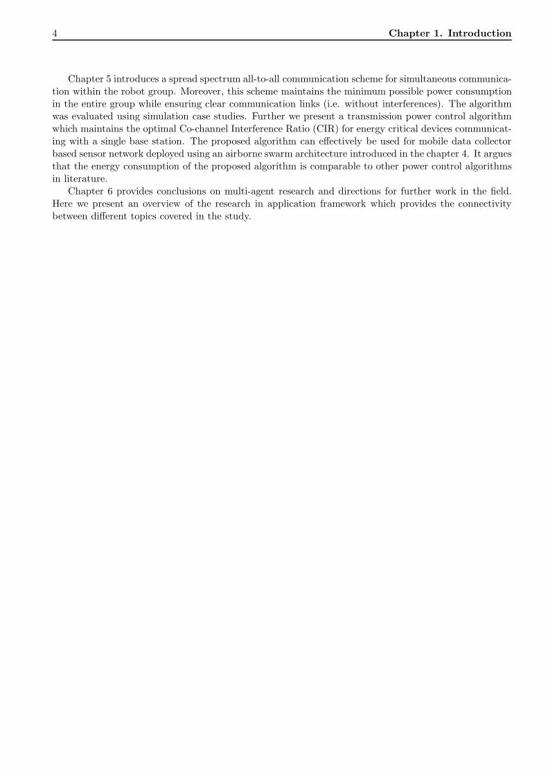
Chapter 5 introduces a spread spectrum all-to-all communication scheme for simultaneous communica-tion within the robot group. Moreover, this scheme maintains the minimum possible power consumptionin the entire group while ensuring clear communication links (i.e. without interferences). The algorithmwas evaluated using simulation case studies. Further we present a transmission power control algorithmwhich maintains the optimal Co-channel Interference Ratio (CIR) for energy critical devices communicat-ing with a single base station. The proposed algorithm can effectively be used for mobile data collectorbased sensor network deployed using an airborne swarm architecture introduced in the chapter 4. It arguesthat the energy consumption of the proposed algorithm is comparable to other power control algorithmsin literature.
Chapter 6 provides conclusions on multi-agent research and directions for further work in the field.Here we present an overview of the research in application framework which provides the connectivitybetween different topics covered in the study.


Chapter 2
Swarm Robots: An introduction
“If every tool, when ordered, or even of its own accord, could do the work that befits it... then therewould be no need either of apprentices for the master workers or of slaves for the lords.” - The Greek
philosopher Aristotle
Robotics and automation of processes are long sought subjects in the human history. Automationapplications date back as far as 4th Century BC, when the Greeks used water clock with movable figures.Evidence of humanoid robots first encounter in Islamic Golden Age (from the middle of the 7th centuryto the middle of the 17th century) when the Arabic inventor Al-Jazari created the first programmablehumanoid robot in 1206. Al-Jazari’s automation was originally a boat with four automatic musicians thatfloated on a lake to entertain guests at royal drinking parties [10]. Moreover, “The Book of Knowledgeof Ingenious Mechanical Devices” by Al-Jazari (1206), reveal several other automation/ robot devicesthat he invented in the early ages of robotic science. In the western world the written history of roboticsarises with the great philosopher Leonardo da Vinci who designed a range of automated machineries forday-to-day life which were found as note book sketches. One of the first documented design of a humanoidrobot called “Mechanical Knight”, was among them, and later it was reconstructed as a miniature version[11].
Among the other early developments in robotics; “Moving anatomy” the mechanical duck by Jacquesde Vaucanson (1738), Designs by Hisashige Tanaka (Karakuri Zui “Illustrated Machinery” was publishedin 1796), Nikola Tesla’s radio-controlled (tele-operated) boat etc; represents major milestones. The word“Robot”, which originates from a Czech word for labor, was first used by Karel Capek on his play Rossum’sUniversal Robots [12]. Since then many science fictions used the term “Robot” to define artificial life andintelligent machines. Issac Asimov (1920-1992) was among the pioneers of the science fiction writerswho popularize the word robot in early stages. Also he defines four rules to be used for robot humaninteractions and still the same rules are accepted globally. Since the “Unimate”, the first industrial robot(developed for the General Motors assembly line in 1961), robotics gain a rapid development inspired bythe development of electronics technology.
Miniature Robots
The concept of miniature robots emerged with the application of robotic devices in the medical, defenseand exploration fields. Applications such as diagnosing and delivering medications to inner body organs,land mine detection, exploration of unknown/hostile terrains (battle fields, collapsed buildings, oceanbed and extra-terrestrial planets) etc; have distinct advantages in employing small, low cost (sometimesdisposable) robots compared with large expensive robots. In general, such system can be effectivelyemployed in situation where: the task covers a region (environmental monitoring - resembling a mobilesensor-network), tasks that are too dangerous (working in an unknown/hostile environment where someunits may destroy), tasks that scales up or down in time, tasks that require redundancy or a mixture ofthe above conditions occur (see [1]). However, the control and coordination of such small robotic devicesto perform a complex task remain a problem for years. Following some interesting studies on social insect
6

Chapter 2. Swarm Robotics: An Introduction 7
Figure 2.1: Some Designs from Leonardos’ Sketches - From left, (1) A sketch of a automated machinegun [13] (2) The outer appearance of the “Mechanical Knight” and (3) the inner mechanism of the knightcontrolling the arms [14]
behavior, robotic scientists developed a new conceptual framework for cooperative miniature robots called“swarm robotics”, which behave like natural swarms such as ants, bees, wasps etc.
Sahin in [1], formally defines the term “Swarm Robotics” as:“Swarm Robotics is the study of how large number of relatively simple physically embodied agents canbe designed such that a desired collective behavior emerges from the local interactions among agents andbetween the agents and the environment.”
Other than that, Gazi and Fidan in [3] describes the swarm or a multi-agent dynamic system as:“A network of a number of loosely coupled dynamic units that collectively reach goals that are difficult toachieve by an individual agent or a monolithic system.”
Distinctive features like decentralized behavior, group learning and distributed sensing demonstratedin such systems make the robots capable of operating in highly hostile environments and unpredictablecircumstances, where centrally controlled robotics systems can simply loose their communications withthe base station. The limitations in computational power, sensing and communication capabilities in smallscale units (especially in micro and nano scale systems) holds a huge barrier against rapid developmentof this technology. However, with recent advances in communication, networking and computing, multi-agent systems have generated a renewed interest among researchers across the world. Moreover, studieson natural swarms have provided the robotics community a great conceptual basis in developing controlalgorithms for decentralized multiple robot coordination.
Natural to Artificial Swarms
Mankind gained a great deal of knowledge by studying the wonders of the mother nature: from a simpletent to a gigantic space station, from a simple hand tool to a large computer network that binds theworld together, there exist the lessons obtained from the nature. There is no exception to the robotics,especially swarm robotics; studies on animal behavior had a lot to share with robotics researchers whowere developing machines to make the life of humans easier.
From pre-historic times, the studies on social insects and birds created the traditional knowledge onnatural disasters and weather predictions. Natural swarms or social foraging animals can be observed inland, air or water. Specially the behavior of insects and other smaller species (such as fish, birds etc)inspired many biological researchers, due to their organized behaviors despite the smaller brain size andlimited sensing capabilities. The robustness, scalability and flexibility of the autonomous behavior (with-out central control) in such a group of insects in achieving complicated tasks (nest building, food finding,attacking enemies etc) contributed many new concepts in artificial intelligence [15, 16, 17], optimization[18, 19, 20, 21] and robotic sciences [1, 22, 23, 24].
Many researchers studied group behavior of animals such as organization of work in ant colonies [25],social foraging models in fish [26], navigation and signaling methods used by ants [27] and in [28] shoalingbehavior of fish with respect to performing an escape mechanism. Mathematical models for the group

8 Chapter 2. Swarm Robotics: An Introduction
behavior developed by Inada in [29] and algorithms governing schooling behavior of fish presented byGrunbaum et al.[30] etc, have inspired the robotics researchers into more refined approaches in swarmingtechniques. For example Keller et. al in [24] analyzed the properties of robot groups having ant-likedecentralized behavior when performing tasks in a collaborative fashion. In [31], the authors present acollaborative cleaning algorithm for a group of robotic vehicles, called “Blind Bulldozing”, which is basedon site preparation of wasps.
In the robotics point of view, the study on flying patterns of a flock of birds by Reynolds [32] becomesthe first of such study which created a mathematical model for the decentralized behavior of a animalgroup. In his study, based on biological research studies on the bird and fish behaviors [33, 34], the flyingmodel uses inter-member communications for collision avoidance and vision-based sensing capabilities.Even though this model is not practical for using directly for actual robotic units, it created a renewedinterest among robotic researchers to investigate social insect behaviors to be used in distributed roboticsystems [3].
2.1 Related Research Topics
The swarm robotic systems and multi-agent dynamic systems have a vast range of research topics andmany of them are associated with the behaviors of social insects. However this section presents the topics/ problems that are relevant to our study. Reviewing the past research literature, several main problemscan be identified with respect to control and coordination of a mobile robotic swarm, namely aggregationand flocking, and pattern formation. In addition to the above, interactions among the robotics group,i.e. communication and sensing, can be considered as other problem area which relates this thesis. In therest of this section, we review some of the relevant past research related to our work.
2.1.1 Aggregation and flocking
In a biological perspective, aggregation (gathering together) is a basic behavior which is demonstratedduring social foraging. Social foraging is basically used to increase success rates in difficult tasks such asfood finding, attacking enemies which could not be accomplished by a single entity. On the other hand,flocking is the collective motion behavior of a large number of interacting agents/robots with a commonobjective, which is a highly demonstrated feature in natural swarms such as birds. Therefore, the swarmrobots deployed in similar missions will essentially demonstrate social foraging behaviors.
Aggregation
Artificial potential field based methods can be considered as the most popular approach in swarm ag-gregation studies. Inspired by the studies on mathematical modeling and simulation of aggregation inbiological swarms [35, 36, 37, 38], Gazi et.al. [39, 40, 41, 42] performed rigorous mathematical analysison the stability of aggregation of swarms using inter-member artificial attraction/repulsion potential fieldbased model. For example, [40], which is the first of the stability analysis studies by Gazi, used theattraction/repulsion function;
g(y) = −y(a− b exp
(−‖y‖2
c
))(2.1.1)
where the motion of an individual agent is modeled by,
xi =M∑
j=1,j �=i
g(xi − xj), i = 1..M. (2.1.2)
Here xi ∈ Rn represents the position of member i and M is the group size. Here the attraction/repulsion
function g(·) represents an artificial social potential function derived from the studies on aggregationbehaviors of biological swarms [37]. In this study Gazi and Passino showed that all the members of theabove swarm moves toward it’s center of mass (x) and all the members converge into a circle with radius

Chapter 2. Swarm Robotics: An Introduction 9
ε =b(M − 1)aM
√c
2exp(−0.5), within a finite time bounded by − 1
2aln
(ε2
2Vi(0)
), where Vi = (1/2)eiT ei
and ei = xi − x. Based on the above studies, in [43, 44, 45] the concept was further enhanced to dealwith the stability of aggregation in different situations such as presence of noise, sensor uncertaintiesand measurement errors. The control architectures of the artificial potential field based approaches arediscussed in detail in the section 2.2.1.
Apart from artificial potential field approaches, behavior based and neural network based methods areamong few successful approaches in achieving swarm aggregation. Soysal and Sahin in [46] introduced abehavior based generic aggregation method using simple probabilistic behaviors of the agents; obstacleavoidance, approach, repel and wait. In this study they conducted systematic experiments to investigatethe behavior of the controller in achieving the aggregation where the robots are using an acoustic sensorto approach or repel from the loudest sound. Similarly Trianni et al., [47] tried to solve the aggregationproblem employing a probabilistic controller using a higher level of abstraction than the sensor readingsand actuator commands. In that study they defined a probability matrix to define the probability ofswitching between behaviors (abstraction of actuator commands) in all the contexts (abstraction of sensordata) and observed the aggregation is possible with a predetermined matrix in a simple sensor-basedsimulation environment. While a rather different approach was introduced by Naruse et al [48] foraggregation of multi-agent system; they used emotion-like two dimensional inner state and affection-likesubjective evaluation of others to perform aggregation behavior.
Bahceci and Shain in [49] study the use and effectiveness of evolutionary methods for developingneural network based controllers for agents in an aggregative swarm robotic system. They tried toachieve aggregation by evolving weights of a neural network with 12 inputs (four inputs to encode thesound values obtained from the speaker and the remaining inputs encodes the infrared sensor readings)and 3 outputs (one for the omni-directional speaker and the other two for controlling the wheels of therobot). Similarly, Trianni et al. in [50] used genetic algorithms to evolve the aggregation behavior byevolving the the weights of a perceptron.
Flocking
To the best of the authors knowledge, the first extensive study in mathematically modeling of a flockingbehavior is by Reynolds in [32], where the flocking behavior of birds were simulated in computer. Inthat study, Reynolds has proposed three basic behaviors for agents which contributes to a global flock-ing behavior, namely (i) separation (Collision avoidance: avoid collisions with nearby flock-mates), (ii)Alignment (Velocity matching: attempt to match velocities with nearby flock-mates), and (iii) cohesion(Flock centering: attempt to stay close to nearby flock-mates). These three simple rules have been usedto develop realistic computer simulations for the flocking behavior of birds. This study was further inves-tigated by Vicsek et al., in [51], in which a self-propelled particle model was used to study the effects ofnoise on the complex particle systems and phase transition from disordered to ordered states.
The flocking models in [32, 51] used “nearest neighbor rules” (where agents adjust their motion basedonly on their nearest neighbors) to achieve global flocking in the absence of centralized coordinationand time varying environments. This concept was further investigated in [52], where a mathematicalanalysis of achieving a common orientation during flocking behavior was performed. Further improvingthe “nearest neighbor rules” concepts, Olfati-Saber in [53] introduces an algorithm for stable flocking ofagents with point-mass dynamics. In this study he used “nearest neighbor rules” and potential functionsfor aggregation and alignment, and provided a comprehensive analysis on the stability of the flockingalgorithms namely free-flocking (flocking where obstacles are not present) and constrained flocking (inthe presence of obstacles).
Apart from the above, Tanner and coworkers in [54, 55, 56] presented flocking behaviors based onartificial potential fields (which depends on the distance between two agents). In [55, 56], they performedextensive analysis of the flocking behavior for systems with point-mass dynamics and in [54] for a systemwith non-holomonic unicycle dynamics.
Rendezvous, on the other hand is another aspect of flocking of natural swarms, which is demonstrated

10 Chapter 2. Swarm Robotics: An Introduction
in birds, fish and mammals; can also be considered as a special form of flocking, where robots arecoordinated to meet at a point or small region [57, 58]. As Lin [58] and Ando [57] proposed in, in theRendezvous problem, each robot tracks the position of neighbors and updates the controller accordingly.Here the neighborhood is defined such that a robot i (Ai) can sense the robot j (Aj), if the distance isless than a constant V and if there is no obstacle in between, i.e. the neighborhood of i (Si) at time t isdefined as; Si(t) ⊆ (Aj |j �= i, ‖xj(t) − xi(t)‖ ≤ V ), where xi represents the position vector of robot Ai.Solutions and mathematical analysis to this problem are provided in [58, 59, 60, 61].
2.1.2 Pattern formation
According to Bayindir and Sahin [2] pattern formation can be defined as the emergence of global patternsfrom local interactions among agents. However Gazi and Fidan in [3] defined pattern formation in moregeneralized form and they introduced three main components of pattern formation; namely (1) formationstabilization and acquisition, (2) formation maintenance and cohesive motion control, and (3) formationreconfiguration and switching. Pattern formation is a widely observed behavior in natural swarms; forexample, a flock of birds in long haul flights generate a “V” shaped formation in order to minimize the airresistance and fatigue of physically weak birds. And it consists of distinct advantages in artificial swarmsor swarm robotics too, facilitating easy maneuvering of the whole swarm when it comes to path planningand strategic positioning (especially in military applications). Unlike in aggregation, the controllers forpattern formation need a formation goal and a control algorithm to achieve that goal, thus consists of amore complex control architecture.
In the pattern generation literature for robotic swarms, several approaches can be identified [62],however in this discussion we classify them into two broad groups based on the control and commandperspectives; namely heterogeneous control and homogeneous control. In this discussion, the heterogeneouscontrol means that the robots/agents are controlled by different command/objective algorithms, and inthe homogeneous controllers, every robot/agent in the group uses the same controller and the objectivefunction. Note that in this discussion we are only considering the decentralized control structures, wherethe members of the swarm do not get control inputs from outside sources, except the objective functionsand sensing (such as location information via RF links, vision based information, proximity informationetc.). However, there exists some centralized control approaches investigated in the swarm literature, forexample, Antolline et. al. introduced a control algorithm for a group of robots in [63] where the controlcommands are send from a base station/ control center.
Among heterogeneous control strategies, leader based control [64, 65, 66, 67, 68, 69], where a virtualleader having a “higher level controller”, which includes the global objective functions, and a group offollowers with a “lower level controller”, which is basically to follow the leader and depends on the controlcommands from the leader, is a common approach. This approach can also be considered as a semi-centralized control approach for pattern formation, since the group is getting commands from the leader(central controller) or based on the behavior of the leader. Another approach in heterogeneous controlis the specific positioning where the objective coordinates of each robot is given before hand, thus eachcontroller consists of different objective functions. In this approach, the formation is predefined and themembers are navigating to occupy the pre-defined positions [69, 70, 71]. Various control techniques aredeveloped to achieve the above objective, among them the behavior based approaches [72] and graph-theory based approaches [52, 53, 65] are significant. Main drawbacks in this approach is that the formationis not scalable and it does not conform with the swarm robotic definitions, due to robustness and flexibilityissues. However this approach is the most reliable one in generating an exact pattern/formation.
In the latter approach (homogeneous controllers), a common function is used to navigate the entireswarm and the system is highly scalable. Among early studies the geometric pattern formation algorithmsintroduced by Sugihara and Suzuki in [73] is a landmark study in which they used a simple controlstructure to control the robot behavior. In that study they presented algorithms to generate; circles(two cases, gathering the robots on the perimeter and populate the circle with robots - FILLCIRCLE ),polygons (two cases, on the perimeter and populate - FILLPOLYGON ) and line segments (based on adecentralized control algorithm). The control algorithms are extremely simple; for example in the circle

Chapter 2. Swarm Robotics: An Introduction 11
generation algorithm, a robot R continuously monitor the positions of a farthest robot R′ and the nearestrobot R′′, breaking ties arbitrarily, and moves as follows in real time;
• Case 1: if d > D, then R moves toward R′,
• Case 2: if d < D − δ, then R moves away from R′,
• Case 3: if D − δ ≤ d ≤ D, then R moves away from R′′,
where d is the distance between R and R′, δ > 0 is a small constant and D is the diameter of the proposedcircle. They have used simulation case studies to evaluate the proposed algorithms. Based on the above,Susuki and Yamashita [74] extended the study to investigate convergence and formation problems, andobtained generalized results for geometric pattern formation issues for a group of mobile robots.
In recent studies for pattern generation, the artificial potential field based methods, and behaviorbased methods have become increasingly popular. The control techniques for these approaches will bediscussed in detail in the section 2.2.
2.1.3 Interactions within the Swarm - Communication and Sensing
Swarm robotics is not always about the control and coordination of mobile agents, it entails the devel-opment of infrastructure for proper functioning such as communication, sensing, processing, power trainsetc. In this section we discuss the studies focused on the communication and sensing for multiple agentsystems or interactions within the swarm. As Bayindir and Sahin classified in there review study [2],the studies on interactions in robotic swarms can be divided into two categories; Interaction via Sensingand Interaction via Communication. Although the discrimination between the two can be difficult, theypropose a guideline based on the information sender side as follows; if the sender in the interaction aimsto give information to other robots intentionally then that study is categorized as “interaction via com-munication” instead of “interaction via sensing”. On the other hand, if robots are sending informationpackets (broadcast or personalized) or interacting to show their status, i.e. switches on/off lights etc, thenthose are considered to be the type of “interaction via communication”.
Interaction via sensing is basically the discrimination of other robots with the environment and isalternatively called as kin recognition. Kin recognition is an important feature of animals in nature.With the help of kin recognition they can perform collaborative tasks and protect themselves from theirenemies better. In swarm robotic studies [50, 75, 46], kin recognition is used as a communication mediumsince some problems (e.g. flocking, chain formation etc) in swarm robotics require discrimination of therobots in the environment to obtain acceptable performance. In this dissertation we do not review theprevious studies in the above research area, “interaction via sensing”. However in the following discussionwe briefly discuss the major communication approaches which can be categorized under “interaction viacommunication”.
A more advanced swarm robotic system, may require direct communication between robots in the formof broadcasting or one-to-one communication. In most of the swarm studies [39, 40, 41] authors assumethat the swarm has a mean of communicating / sharing valuable information such as state information,however they do not elaborate the underlying communication protocol. While some studies give moreinformation on the communication architecture than the control aspects of the robots. For example,Nouyan and Dorigo in [76] implemented a chain formation behavior using a status indication in the formof a LED ring around their body. In that study the colors of the LED ring (red, green and blue) indicatedifferent status of the member and it can be used by the neighboring robots to determine their activities.Similar to above, Grob et al., [77] studied a self-assembly problem in which the robots discriminate themembers connected to the seed using a bi-color LED ring around their body.
Apart from the above there exists some studies where the communication / interaction uses the en-vironment as the communication media, which are categorized as interaction via environment [2]. Thesestudies are based on the communication approaches used by biological swarm, such as pheromone com-munication of ants. Pheromones is a chemical that ants lay on the ground. When an ant finds food, itwill leave a trail along the ground on its way back to home, which in a short time other ants will follow.
12 Chapter 2. Swarm Robotics: An Introduction
In the swarm robotic studies [78, 79, 80, 81] the same concept was used for communication in a roboticswarm where they used artificial pheromones.
In the swarm robotic literature, one could not find a wireless communication approach (i.e. Infraredor RF based) explicitly for swarm robots. However the studies in wireless sensor network, where ad-hoc connected set of node communicate with each other to share valuable information, can be used forcommunication within a robotic swarm. A review of such communication methods developed for wirelesssensor networks is presented in chapter 5.
2.2 Coordination and control approaches in swarms
Swarm robotics and the rest of the robotic systems can be clearly distinguishable based on the controlarchitecture. The autonomous behavior of agents without a central control is the key factor in a roboticswarm. The central control based robotic groups (which includes leader based strategies) are prone tomany drawbacks; such as higher computational cost and complexity, sensitivity to loss of some agents(e.g. leader/central commanders in leader based systems), communication delays between the controlcenter/leader and the other agents, feasibility of processing entire network information by the centralunit. These are disadvantageous to operate in hostile and changing environments[3]. However, one canobserve that there is significant number of literature on centralized control architectures of swarm robots(see [63, 64, 65]). In this section we briefly discuss the major control and coordination approached foundin swarm literature, while mainly concentrating on approaches similar to ours [4, 5, 6, 7].
2.2.1 Potential Field Based Approaches
Use of artificial potential fields for multiple robot navigation, first introduced by Reif and Wang in [82],have been extensively studied in the literature [39, 40, 41, 83, 84, 85].
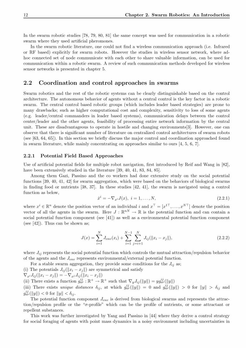
Among them Gazi, Passino and the co workers had done extensive study on the social potentialfunctions [39, 40, 41, 42] for swarm aggregation, which were based on the behaviors of biological swarmsin finding food or nutrients [38, 37]. In these studies [42, 41], the swarm is navigated using a controlfunction as below,
xi = −∇xiJ(x), i = 1, . . . , N, (2.2.1)
where xi ∈ Rn denote the position vector of an individual i and x� = [x1�, . . . , xN�] denote the position
vector of all the agents in the swarm. Here J : RnN → R is the potential function and can contain a
social potential function component (see [41]) as well as a environmental potential function component(see [42]). Thus can be shown as;
J(x) =N∑
i=1
Jenv(xi) +N−1∑i=1
N∑j=i+1
Jij(‖xi − xj‖), (2.2.2)
where Jij represents the social potential function which controls the mutual attraction/repulsion behaviorof the agents and the Jenv represents environmental/external potential function.
For a stable swarm aggregation, they provide some conditions for the Jij as;(i) The potentials Jij(‖xi − xj‖) are symmetrical and satisfy∇xiJij(‖xi − xj‖) = −∇xjJij(‖xi − xj‖)(ii) There exists a function gij
ar : R+ → R
+ such that ∇yJij(‖y‖) = ygijar(‖y‖)
(iii) There exists unique distances δij , at which gijar(‖y‖) = 0 and gij
ar(‖y‖) > 0 for ‖y‖ > δij andgijar(‖y‖) < 0 for ‖y‖ < δij .
The potential function component Jenv is derived from biological swarms and represents the attrac-tion/repulsion profile or the “σ-profile” which can be the profile of nutrients, or some attractant orrepellent substances.
This work was further investigated by Yang and Passino in [44] where they derive a control strategyfor social foraging of agents with point mass dynamics in a noisy environment including uncertainties in

Chapter 2. Swarm Robotics: An Introduction 13
the sensing environment as well as the relative positions between agents. In addition to the controllerused in [41, 42], the agents in this approach tries to move toward the center of the swarm and match itsvelocity with the average velocity of the group. The motion of the swarm in [44] was controlled by;
xi = −kipe
ip − ki
v eiv − kvi −∇xiJ(x), i = 1, . . . , N (2.2.3)
where, eip = eip − dip and eiv = eiv − di
v. In above expression dip and di
v represents the uncertainties inposition and velocity measurements, and eip = xi − x, eiv = vi − v are relative position and velocity ofith agent with the center of the swarm (x, v). The ∇xiJ(x) in the above represents the noisy gradient,which is similar to that of [41, 42]. They have shown that the above swarm demonstrates stable foragingdespite the uncertainties in sensing/measurements.
Similar to above study Olfati-Saber in [53] introduced a control strategy for swarm aggregation wherethe velocity matching term is matching the velocities of the neighboring members only. This is basedon the flocking algorithm of Reynolds [32]. The velocity matching part of the controller (uvi) is in thefollowing form;
uvi = −mi∑j∈ℵi
kijv (x)(vi − vj), i = 1, . . . , N. (2.2.4)
Here the neighboring members of i are defined as; ℵi = {j ∈ V : ‖xi − xj‖ < r}, where r ∈ R+.
Similarly to the attractive/repulsion functions in [86, 41, 42, 44, 53], artificial potential functions arebeing used for swarm aggregations, formation and other multiple-robot coordination and control tasks.Some of the work directly address the issues of collisions between agents, using unbounded repulsionfunctions to guarantee collision avoidance [86, 87], where the inter-individual repulsion force is in theform of;
gr(‖xi − xj‖) =c
‖xi − xj‖2, (2.2.5)
which goes to infinity as the distance between two members approaches zero.Moreover, researchers investigate numerous issues in a swarm using a potential field based controller,
such as cohesiveness of the group, bounds of the swarm size and the motion of the group achieving theobjectives (formation, flocking). Lyapunov-like methods are usually used for analysis resulting in conser-vative bounds. Furthermore, in the analysis, some studies [40, 41, 86, 44] assumed that each individualagent knows the relative positions of the entire swarm, which become unrealistic for biologically inspiredcontrol approach. In a biological swarm, each agent can only observe the positions of the neighboringmembers, which is the case with the Reynolds approach [32].
In all above control approaches the swarm is modeled to have higher-order agent dynamics, i.e. pointmass dynamics and single integrator model (see Remark 2.2.1), where the motion dynamics of the agentdoes not correspond to any real-world vehicle or a motion platform. However, the results obtained are ofhigh value, since given the motion characteristics of the swarm, one can design a controller so that it worksas with higher-order models. Sliding mode control is a such approach in which a switching controller withhigh enough gain is applied to suppress the effects of modeling uncertainties and disturbances, and theagent dynamics are forced to move along a stabilizing manifold called sliding manifold. Gazi in [41] useda similar technique to control a swarm with fully-actuated agent model with uncertainty (see Remark2.2.2). In the sliding mode control approach, it is possible to design each of the control inputs ui toenforce satisfaction of the trajectories generated by the higher-level models and therefore recover fromthe deficiencies due to mismatching between the actual and modeled agent dynamics [41]. The slidingmanifold used in [41] is in the following form,
si = xi + ∇xiJ(x) = 0, i = 1, . . . , N, (2.2.6)
where x� = [x1�, . . . , xN�]. Then by choosing the control inputs as;
ui = −ui0(x)sign(si) + fk
i (xi, xi), (2.2.7)

14 Chapter 2. Swarm Robotics: An Introduction
where sign(si) = [sign(s1), . . . , sign(sN )]�, and choosing gain ui0(x) of the control input as
ui0(x) > Mi
(1M i
fi(xi, xi) + Ji(x) + εi), (2.2.8)
one can guarantee that si�si < −εi‖si‖ and that sliding mode occurs. In above Mi,M i and fi(xi, xi) arethe known bounds on the uncertainties and disturbances, Ji(x) is the computable bound on the potentialfunction derivative and εi > 0 is an arbitrary constant.
Remark 2.2.1. In the single-integrator motion model, the motion of the ith agent is given by xi = ui. In
the point-mass dynamics, the motion of the ith agent is given by xi =1miui. Here mi is the mass of the
agent and ui represents the control input for the agent.
Remark 2.2.2. The fully actuated agent model is a more realistic model for agent / robot / vehicle dynamicsthan single-integrator and point-mass models and the motion of such system is governed by;
mixi + f i(xi, xi) = ui, i = 1, . . . , N. (2.2.9)
Here, xi,mi and ui represent the position, mass and control input of the agent respectively, and f i(xi, xi) ∈R represents the centripetal, Coriolis, gravitational effects and additive disturbances.
2.2.2 Artificial Physics Based Approaches
Artificial physics based approach for control and navigation of multiple robots is introduced by Spearsand Gorden in [88], and further enhanced by Spears, Spears-Gordon1 and co-workers in [88, 75, 89, 90,91, 92, 93]. In the review study [3], Gazi and Fidan classify this approach as a subclass of the potentialfield based control approaches. Artificial physics framework, alternatively called “physicomimetics”, isbased on the fundamental laws of physics, particularly mechanics such as Newton’s laws of motion, andthe robotic behaviors that are similar to those shown by solids, liquids, and gases. They proposed solidformations for distributed sensing tasks, liquids like behavior for obstacle avoidance tasks and gas likebehavior for coverage tasks, such as surveillance and sweeping.
The concept behind the “physicomimetics” framework is elegantly simple. In essence, virtual physicalforces drive a multi-agent system to a desired configuration or state. The desired configuration (state) isa one that minimizes overall system potential energy - similar to the artificial potential field framework.In macroscopic level, the system acts as a molecular dynamics (F = ma) simulation. At an abstractlevel, artificial physics treats the agents as physical particles (point mass agents) in a 2D or 3D space.In their framework, the state of each particle (agent) is calculated using the laws of physics at eachtime step, based on the forces applied to a particular agent. Moreover, they have used novel methodsfor the analysis, which differs from Lyapunov based methods, common in artificial potential field basedapproaches [39, 40, 41]. In some cases provides experimental evidence of the system behavior using smallinexpensive robots [75]. Another important aspect in their study is the chemical plume tracing [92, 93, 91]which is particularly important in security and surveillance applications.
In their basic framework they defined an inter-agent attractive/repulsive function;
Fij =Gmimj
rpij
≤ Fmax (2.2.10)
where G is the “gravitational constant”, mi,mj are the masses of agents i and j, rij is the distancebetween the agents i and j, and p ∈ [−5, 5] is a user-defined variable. Moreover, they have defined thatthe force Fij is attractive when r > R and repulsive when r < R. In above equation Fmax represents themaximum force that can be applied on any particle.
1Diana Gordan later become Diana Spears
Chapter 2. Swarm Robotics: An Introduction 15
2.2.3 Behavior Based Approaches
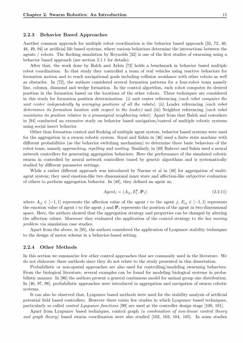
Another common approach for multiple robot coordination is the behavior based approach [32, 72, 46,48, 49, 94] or artificial life based systems, where various behaviors determine the interactions between theagents / robots. The flocking simulation by Reynolds [32] is one of the first studies of swarming using abehavior based approach (see section 2.1.1 for details).
After that, the work done by Balch and Arkin [72] holds a benchmark in behavior based multiplerobot coordination. In that study they controlled a team of real vehicles using reactive behaviors forformation motion and to reach navigational goals including collision avoidance with other robots as wellas obstacles. In [72], the authors considered several formation patterns for a four-robot team namelyline, column, diamond and wedge formation. In the control algorithm, each robot computes its desiredposition in the formation based on the locations of the other robots. Three techniques are consideredin this study for formation position determination: (i) unit center referencing (each robot computes theunit center independently by averaging positions of all the robots), (ii) Leader referencing (each robotdetermines its formation location with respect to the leader) and (iii) Neighbor referencing (each robotmaintains its position relative to a preassigned neighboring robot). Apart from that Balch and coworkersin [94] conducted an extensive study on behavior based navigation/control of multiple robotic systemsusing social insect behavior.
Other than formation control and flocking of multiple agent system, behavior based systems were usedfor the aggregation in a swarm robotic system. Soyal and Sahin in [46] used a finite state machine withdifferent probabilities (as the behavior switching mechanism) to determine three basic behaviors of therobot team, namely approaching, repelling and waiting. Similarly, in [49] Bahceci and Sahin used a neuralnetwork controllers for generating aggregation behaviors. Here the performance of the simulated roboticswarm in controlled by neural network controllers tuned by genetic algorithms and is systematicallystudied by different parameter settings.
While a rather different approach was introduced by Naruse et al in [48] for aggregation of multi-agent system; they used emotion-like two dimensional inner state and affection-like subjective evaluationof others to perform aggregation behavior. In [48], they defined an agent as;
Agenti = (Aij , Eki ,Pi) (2.2.11)
where Aij ∈ [−1, 1] represents the affection value of the agent i to the agent j, Eij ∈ [−1, 1] representsthe emotion value of agent i to the agent j and Pi represents the position of the agent in two-dimensionalspace. Here, the authors showed that the aggregation strategy and properties can be changed by alteringthe affection values. Moreover they evaluated the application of the control strategy to the box movingproblem via simulation case studies.
Apart from the above, in [95], the authors considered the application of Lyapunov stability techniquesto the design of motor scheme in a behavior-based setting.
2.2.4 Other Methods
In this section we summarize few other control approaches that are commonly used in the literature. Wedo not elaborate these methods since they do not relate to the study presented in this dissertation.
Probabilistic or non-spatial approaches are also used for controlling/modeling swarming behaviors.From the biological literature, several examples can be found for modeling biological systems in proba-bilistic manner. In [96] the authors present a general continuous model for animal group size distribution.In [46, 97, 98], probabilistic approaches were introduced in aggregation and navigation of swarm roboticsystems.
It can also be observed that, Lyapunov based methods were used for the stability analysis of artificialpotential field based controllers. However there exists few studies in which Lyapunov based techniques,particularly so called control Lyapunov functions [99] are used at the controller design stage [100, 101].
Apart from Lyapunov based techniques, control graph (a combination of non-linear control theoryand graph theory) based swarm coordination were also studied [102, 103, 104, 105]. In some studies

16 Chapter 2. Swarm Robotics: An Introduction
Asym ptotically StableStable
Unstablex0
O
R
r
H(R)
H(A)
S(A)
S(R)
S(r)
Figure 2.2: Stability Regions in the Lyapunov Method
[102, 105] a leader based formation control systems (moving reference) were used while in some others[103] distributed control techniques were used. The virtual leader concept is also a common approach inmultiple robot formation control and in some studies the virtual leader controls the other members of thegroup while in others the virtual leader acts as a moving reference point that influences the member inits neighborhood [67, 65, 72].
Besides the work mentioned above, various other approaches can be found in the literature in non-linear control frame works, such as neural networks, dynamic inversion, back-stepping, adaptive control,output regulation etc. However we avoid the details of the control strategies and models involved in them.
2.3 Mathematical Background
The multiple robot coordination and communication architecture introduced in this thesis uses severalmathematical concepts in deriving the control algorithms and in the analysis sections. This sectionpresents a basic introduction for some underlying mathematical and analytical techniques used in thethesis.
2.3.1 Lyapunov Stability
The Lyapunov Stability criteria2, first introduced by Russian mathematician Aleksandr MikhailovichLyapunov (1857 − 1918), is an approach to determine the stability of an autonomous system in the form
x = f(x), and f(0) = 0 (2.3.1)
where x = [x1, . . . , xn]� denotes a vector containing state of the system, for example positions andvelocities. Before introducing the Lyapunov stability theorems we introduce few definitions on the stabilityand control functions.
Definition 2.3.1 (Positive/Negative Definite/Semi-Definite Functions).A continuously differentiable function W : R
n → R+ is said to be positive definite in a region U ∈ R
n
that contains the origin if W (0) = 0, and W (x) > 0, ∀x ∈ U and x �= 0. W (x) is said to be positivesemi-definite if W (0) = 0, and W (x) ≥ 0, ∀x ∈ U and x �= 0.Conversely, the function W (x) is negative definite if W (0) = 0, and W (x) < 0, ∀x ∈ U and x �= 0, andnegative semi-definite if W (0) = 0, and W (x) ≤ 0, ∀x ∈ U and x �= 0.
Stability of an Autonomous System
Consider an autonomous system as in equation (2.3.1) where its stability is sought at the state x = a.For the convenience of defining the stability modes, we transfer the sought state to the origin using a
2Note that the contents (definitions and theorems) of this section is produced based on the “Stability by Lyapunov’s DirectMethod With Applications” by Joseph LaSalle and Solomon Lefschetz [106].

Chapter 2. Swarm Robotics: An Introduction 17
transformation x∗ = x− a and by replacing x∗ with x, we have the general form x = f(x) and f(0) = 0.Defining S(R) as the spherical region ‖x‖ < R, H(R) as the spherical region ‖x‖ = R, and SR
r as theclosed spherical annular region defined by r ≤ ‖x‖ ≤ R. Moreover, assume the basic existence theorem
holds for equation (2.3.1) and the partial derivatives∂fi
∂xjall exist and are continuous in Ω : ‖x‖ < A,
where A is the radius of the sphere H(A). Let g+ be the part of g described by x(t) when t ≥ 0 and g−
be the part of g described by x(t) when t ≤ 0, where g is the trajectory of x(t). Then the stability of theorigin is defined as follows (see Figure 2.2);Stable, whenever for each R < A there is an r ≤ R such that if a path g+ initiates at a point x0 of thespherical region S(r) then it remains in the spherical region S(R) ever after, i.e. the path starting in S(r)never reaches H(R) of S(R),Asymptotically Stable, whenever it is stable and in addition every path g+ starting inside someS(R0), R0 > 0, tends to the origin as time increases indefinitely, andUnstable, whenever for some R and any r, no matter how small, there is always in the spherical regionS(r) a point x such that the path g+ through x reaches the boundary sphere H(R).
Lyapunov Stability Criteria
Lyapunov stability is based on a special type of function called the Lyapunov function, which is definedas follows.
Definition 2.3.2 (Lyapunov function).A positive definite scalar function V (x) with the following properties;
1. V (x) is continuous together with its first partial derivatives in a certain open region Ω about theorigin
2. V (0) = 0
3. Outside the origin (and always in Ω) V (x) is positive
4. The first partial derivative of V (x), is negative semi-definite in Ω, i.e. V ≤ 0
is called a Lyapunov function.
Then the Lyapunov Stability Theorems are as follows;
Theorem 2.3.1 (Lyapunov Stability Theorem).If there exists in some neighborhood Ω of the origin a Lyapunov function V (x), then the origin is stable.
Theorem 2.3.2 (Lyapunov Theorem for Asymptotic Stability).If there exists in some neighborhood Ω of the origin a Lyapunov function V (x) and the V is negativedefinite, then the origin is asymptotically stable.
In the essence, if one can find (create) a function V (x) that satisfy above criteria for an autonomoussystem in the form described by equation (2.3.1), then the system is stable. However, this does not meanthat if a particular V (x) does not satisfy the Lyapunov criteria, then the system is unstable.
In many swarm robotic research studies the Lyapunov stability is used to determine the stability of acontroller for convergence [39, 40, 41].
LaSalle Theorem: An Extension to the Lyapunov Criterion
Extending the Lyapunov Stability criteria, LaSalle and coworkers have introduced a theorem for deter-mining stability for systems with V negative semi-definite and defined as follows;

18 Chapter 2. Swarm Robotics: An Introduction
Theorem 2.3.3 (Extended Lyapunov Stability Theorem ).Let V (x) be a scalar function with continuous first partial derivatives. Let Ω1 denotes the region whereV (x) < l. Assume that Ω1 is bounded and that within Ω1: V (x) > 0 for x �= 0, and V (x) ≤ 0. Let R bethe set of all points within Ω1 where V (x) = 0, and let M be the largest invariant set in R. Then everysolution x(t) in Ω1 tends to M as t→ ∞.
As a special case, if V (x) = 0 in R only for x = 0 then the system is locally asymptotically stable atthe origin.
2.3.2 Complex Integration and Winding Number Theorem
In this study we are using complex domain to represent the state of the robots in 2D space in order tobenefit some special features of complex integration and complex analysis. This section aims in deliveringthe fundamental concepts behind the complex number theories used in the next two chapters. A functionin complex domain is defined as: a function f is a complex function whose domain Ω is a subset of complexplane and whose range is also a subset of complex plane. In other words, w = f(z) = u(z) + iv(z) is acomplex function, where u(z) = u(x, y) and v(z) = v(x, y) are real-valued functions and x, y ∈ R.
In complex analysis the basic form of integration is the line integral, where a function f : U → C
integrated along a path γ : [a, b] → U is defined as∫γf(z)dz (2.3.2)
where U ⊂ C or, if the contour γ is closed then the integration is represented as∮γf(z)dz. (2.3.3)
This can also be defined, specially in numerical integration approaches, by subdividing the range [a, b]into n intervals (i.e. [a, b] = (t0, . . . , tn) in the form,∫
γf(z)dz ≡
n∑k=1
f(γ(tk))γ(tk) =n∑
k=1
f(γ(tk)) (γ(tk) − γ(tk−1)) (2.3.4)
and the accuracy of the integral improves with n → ∞. Note that in the above expression dz = γ(tk) =γ(tk) − γ(tk−1). Moreover in complex analysis, the length of a line is defined as;
l(γ) =∫
γ‖dz‖ (2.3.5)
and can be extended to find the circumference of a closed contour as,
l(γ) =∮
γ‖dz‖. (2.3.6)
The numerical representation of the above is in the form (using similar notation as above)
l(γ) =∮
γ‖dz‖ ≡
n∑k=1
‖γ(tk) − γ(tk−1)‖ (2.3.7)
and since the intervals are equal (i.e. ti = ‖γ(t1) − γ(t0)‖ = · · · = ‖γ(tn) − γ(tn−1)‖), we can write theabove expression as,
n∑k=1
‖γ(tk) − γ(tk−1)‖ = n ti (2.3.8)

Chapter 2. Swarm Robotics: An Introduction 19
γ γ
γ
(a) Simple Closed Path (b) Open Path (c) Closed Non-Simple Path
Figure 2.3: Different Contour Types - In this study we are considering only simple close contours asthe pattern generation envelope, however if one can generate non-simple contours for the pattern bycombining several simple closed contours as explained in the chapter 4
Cauchy Integral Theorem and Cauchy Integral Formula
We look in to some interesting results for complex integration introduced by Cauchy namely the Cauchy’sIntegral Theorem and Cauchy’s Integral Formula. The Cauchy’s Integral Theorem is for a line integralalong a simple-closed path (see Figure 2.3) and defined as,
Theorem 2.3.4 (Cauchy’s Integral Theorem).If f(z) is analytic in a simply connected domain D, then for every simple closed path C in D,∮
γf(z)dz = 0. (2.3.9)
Theorem 2.3.5 (Cauchy’s Integral Formula).Let f(z) be analytic in a simply connected domain D. Then for any point z0 ∈ D and any simple closedpath C in D that encloses z0, ∮
γ
f(z)z − z0
dz = 2πif(z0). (2.3.10)
In this study, we use functions having a contour integral in the form,∮γf(z)‖dz‖ (2.3.11)
and the numerical representation of such function is
W (z) =∮
γf(z)‖dz‖ =
n∑k=1
f(zk) (2.3.12)
where zk = γ(tk) represents a point on the path γ. For example if we use a function f(z) = z− z0, wherez0 ∈ C is a constant, then the W (z) represents the vector sum of z − z0 for all the point on the path γ(see Figure 2.4).
Based on the above results of Cauchy there exists another important result on complex integrationcalled Winding Number defined as follows,
Definition 2.3.3 (Winding Number).The winding number of a contour γ about a point z0, denote by n(γ, z0), is defined as
n(γ, z0) =1
2πi
∮γ
dz
z − z0(2.3.13)
which gives the number of times γ curve pases (counterclockwise) around a point.
Above definition can be used to determine the position of a point (z0) with respect to a contour (γ)in the complex plane, i.e. if the winding number ‖n(γ, z0)‖ > 0 then the point z0 is inside the contour γand if ‖n(γ, z0)‖ = 0 then the point lies outside the contour. We use this result in defining the controllerfor swarm coordination in the following chapters.

20 Chapter 2. Swarm Robotics: An Introduction
z0
z1z2z3
z4
zk
zn
γ
Figure 2.4: Vectors Representing (zk − z0)
2.3.3 Perron-Frobenius Theorem
The Perron-Frobenius Theorem is a theorem in matrix theory about eigenvalues and eigenvectors of areal positive n× n matrix, and it is defined as follows [107, 108];
Theorem 2.3.6 (Perron-Frobenius Theorem). Let A = aij ∈ Rn×n and suppose that A is irreducibleand non-negative. Then
• ρ(A) > 0;
• ρ(A) is an eigenvalue of A;
• There is a positive vector x such that Ax = ρ(A)x; and
• ρ(A) is an algebraically (and hence geometrically) simple eigenvalue of A;
where ρ(A) is the spectral radius.
In other words, the eigenvalue r = ρ(A) has following properties; |λ| ≤ r where λ is any othereigenvalue of A, and r can be estimated using;
mini
∑j
aij ≤ r ≤ maxi
∑j
aij . (2.3.14)
2.4 Problem Statements
In this thesis two main problems in the swarm robotics are considered: geometric pattern generationand communication. In the geometric pattern generation problem, which is the main contribution inthe thesis, we develop an artificial force based control/navigation algorithm which populates a group ofrobots into a pre-determined contour. In the communication problem, which acts as a supplementarywork to improve the pattern generation algorithm, an all-to-all wireless communication power controlalgorithm is introduced such that all the members in the group can communicate with every other memberinstantaneously and simultaneously. Apart from that we also introduces a nodal communication powersaving algorithm for mobile data collector based data collection scenario, which represents an importantapplication of our main study. In the following section we compare our objectives with existing literatureto emphasis the novel features of our architecture.
2.4.1 Geometric Pattern Generation Problem
In this section we compare the proposed method for geometric pattern generation with the existingapproaches. First define the problem: simply “populate a given number of robots/ agents inside a givencontour”, and as secondary objectives; avoid inter-agent collisions, scalability, stability, and decentralizedbehavior.

Chapter 2. Swarm Robotics: An Introduction 21
As described in 2.1.2, the controller we are interested is “decentralized”, and “homogeneous” such thatit exclude virtual leader based approaches [65], controllers which assign specific locations for robots [64, 71]and remote information processing (for localization and navigation) techniques [63]. Moreover, we do nottry to make a replica of a natural swarm [40] (such as social insects, birds etc) behavior. However theobjective is to inherent the favorable aspects of such behaviors while improving the quality of ultimate goalof pattern generation. In doing so we assume a robotic system with advanced self-localization techniquesand communication architecture, which could not be observed in natural swarms.
The self-localization capability means that the robot is equipped with a sensing system which enableit to determine its position with respect to a global land mark. In a real robotic system this could beradar based, vision based, inertial techniques (using accelerometers) or GPS based, which could achievethe above objective. One may argue that the GPS based systems are not decentralized since it uses aglobal information source, however in a GPS based localization system the global source do not calculatethe position of the receiver. Instead the receiver does all the calculation based on continuous data codesfrom three or more satellites. Thus we argue that it is decentralized as long as the processing is done atthe node and the global information codes do not send specific code to each robot.
Artificial force based and potential field based approaches are extensively studied in the swarm litera-ture. However our approach is somewhat different from them due to dynamic calculation of the potentialfield and the artificial forces. Moreover, this approach enables the robots to generate virtually any shapewhich can be defined by a simple and closed contour (not necessarily be a mathematical expression).Under the proposed control architecture we populate a given shape (rather than the periphery as in[43, 74, 109, 85]) with the swarm without using predefined positions(unlike in [64][71]) where the shapescan be described by a mathematical function (contour). The only relevant previous work which relatesto this dissertation is the study by Sugihara and Suzuki in [73], in which they populate a group of agentsinto a simple geometric shape, i.e. circles and polygons. However, that algorithm lacks the ability ofgenerating arbitrarily defined shapes which could potentially be important in a robotic swarm deployedin a mission critical operation. The figure 2.5 compare different formation strategies encounter in pastswarm robotic literature.
(a) (b) (c) (d)
Figure 2.5: Different Shape Formation Strategies - The sub figure (a) represents a scenario where therobots/agents are placed along the contour. This is particularly important in enclosing a target i.e. inescorting tasks. In the “Contour-Fill” (sub figure (b)) type formation, the area inside the target contouris filled/ populated with the robots. In the application domain this have multitude of applications such asexploration, sensor network deployment, weapon/ vehicle deployment in military applications etc, whichbenefits the scalability and the robustness of the formation in addition to the advantages of covering angeographical area. Sub figure (c) represents a di-graph based formation strategies, which are based ongraph theory based approaches. In sub figure (d) the technique used in [71] is illustrated where each robotis assigned with a specific position in the formation and the robot is navigated to occupy that place.

22 Chapter 2. Swarm Robotics: An Introduction
2.4.2 Communication problem
We investigate the communication problem of such a swarm of robots in which all the robots are com-municating with each other at the same time[9]. Although many approaches (media and methods) canbe observed for the communication, in this approach we use Radio Frequency wireless communications.Moreover, in the application-domain of the communication problem, we propose a method for power-efficient single-hop data collection from a randomly dispersed set of nodes where multi-hop network is notfeasible[8].
As discussed in section 2.1.3, the interactive approaches based on wireless communication are notsufficiently discussed in the swarm studies. The one-to-one communication feature in wireless sensornetworks, i.e. the communication based on the node ID and the routing of information via a routingtables, makes it impractical and unsuitable for swarm robotics where the network is extremely dynamic.Moreover the node ID based communication limits the scalability and robustness of the network sincethe changes in node structure affects the communication protocols. In our study, the above problem iseliminated by introducing a all-to-all broadcasting type wireless network which can be used in swarmrobotics as well as in wireless sensor networks.


Chapter 3
Geometric Pattern Generation in aMultiple Robot System
This chapter introduces the main assertion of the research which lays the foundation to the rest of thethesis. The shape formation algorithm introduced here navigates a group of robots into a pre-determinedshape contour and spreads them within that shape. The controller uses artificial formation forces actingon the robots, forces due to the target shape as well as due to neighboring members, which eliminateinter-member collisions and ensure smooth navigation of the group.1
First we introduce the mathematical model for the robotic system together with the artificial forcefunctions which define the controller. Then a behavioral analysis of the group of mobile robots under theproposed controller was performed and the assertions were verified using computer simulations . In themathematical analysis, we provide conditions for selecting the controller parameters which determinesthe cohesiveness, stability and the effectiveness of the formation strategy. For the analysis, the followingwere assumed;
• Agents/members have identical physical properties (such as mass, mobility etc.)
• Agents/members are point masses i.e. without any physical dimensions and demonstrate point massdynamics
• Agents/members have instantaneous and error free localization capabilities
• The communication network of the members can transmit data to all the members within the groupinstantaneously, i.e. without delay
• Agents/members operate on a 2D plane without obstacles
Basically the above assumptions were made in order to reduce the system complexity in the controlleranalysis phase and to highlight the basic formation algorithm. But in subsequent chapters of the thesiswe relax these assumptions and use a swarm model which closely resembles a platoon of real world roboticvehicles.
3.1 Mathematical Model
This section introduces the mathematical model of the multi-agent dynamic system together with theartificial force functions.
1Please note that the material presented in this chapter was published as a journal paper :Ekanayake, S.W. and Pathirana,P.N., “Formations of Robotic Swarm - An Artificial Force Based Approach,” International Journal of Advanced RoboticSystems, Vol. 6, No. 1 (2009) pp. 7-24
24

Chapter 3. Geometric Pattern Generation in a Multiple ... 25
Desired Target Contour
M embers of the robotic group
(a) Initial State (b) Final State
Figure 3.1: Ultimate Objective of the Multiple Robot System - The mobile robots scatters in the space (subfigure (a)) are gathered into a clearly defined contour (sub figure (b) bottom). The robots are navigatedfrom the artificial forces which are from other robots, shape contour as well as from friction (sub figure(b) top)
Remark 3.1.1. Throughout this dissertation, the terms member or agent represent a member in the swarm,while the terms swarm or multi-agent system represents the complete swarm. Also, we use C to representcomplex number, R for real number and R
+ to represent positive real number. Further, we use �(.) and�(.) to represent imaginary and real component of a complex number respectively.
Remark 3.1.2. For easy representation of vector based force components with contour integrals and forease of analysis we used the complex plane instead of the cartesian plane. But in implementing thealgorithm in real robots, the cartesian vector based representations can be adopted.
3.1.1 Shape formation algorithm
Consider a swarm or multi-agent system consisting of N number of identical members operating in twodimensional Euclidean space. In this context we consider the problem of controlling and positioning theabove swarm into a shape bounded by a simple closed contour γ defined in the complex plane, whilespreading members inside the contour uniformly (see Figure 3.1).
The state of the member i is described by
Xi =
⎡⎢⎢⎣zi
zi
⎤⎥⎥⎦ , (3.1.1)
where zi ∈ C, represents the position of the ith member in 2D complex plane. Let z be a point on γ, i.e.z ∈ γ. Before stating the swarm model, we define α =
[1 0
]and β =
[0 1
]. Then the state of
the whole swarm, x =[X1 X2 X3 ... XN
]Tis determined by the continuous time dynamic model
described by,
x = Ax+Bu, (3.1.2)

26 Chapter 3. Geometric Pattern Generation in a Multiple ...
Y −Coordinate
X −Coordinate
Rep
ulsi
ve F
orce
Mag
nitu
de
(a)
X −Coordinate
Y −Coordinate
Rep
ulsi
ve F
orce
Mag
nitu
de
(b)
X −CoordinateY −Coordinate
Rep
ulsi
ve F
orce
Mag
nitu
de
(c)
Figure 3.2: Artificial Repulsion Force Field for different shape contours
where
A = diag(A)
N×N, (3.1.3)
B =1mdiag
(B)
N×N(3.1.4)
with
A =
⎡⎣ 0 1
0 0
⎤⎦ & B =
⎡⎣ 0
1
⎤⎦ . (3.1.5)
In (3.1.3), m is the mass of a member. According to our assumptions, notice that each member’s positioninformation (
[αX1 αX2 . . αXN
]) is available to the communication network. In other words, all
the members know the location matrix without a delay.The control input u in (3.1.2) consists of,
u =[u1 u2 u3 ... uN
]T(3.1.6)
whereui = Fi,a + Fi,r + Fi,m − Fi,f . (3.1.7)
The artificial formation forces are described as follows;
Artificial Attraction Force
Fi,a, attraction force on the ith member from the shape,
Fi,a := ka (1 − n(γ, αXi))∫
γ(z − αXi) ‖dz‖ . (3.1.8)
Artificial Repulsion Force
Fi,r, artificial repulsion force on the ith member from the shape,
Fi,r := kr n(γ, αXi)∫
γ
[(αXi − z)‖αXi − z‖3
]‖dz‖ . (3.1.9)
In above equations, n(γ, zi) represents the Cauchy Winding Number of γ about zi ∈ C, having thefollowing from,
n(γ, zi) =1
2πi
∫γ
dz
z − zi

Chapter 3. Geometric Pattern Generation in a Multiple ... 27
Remark 3.1.3. Clearly
n(γ, αXi) ={
1 when member i is inside γ0 when member i is outside γ
,
ensures that the term Fi,a in (3.1.7) vanishes only if the member is inside the contour and term Fi,r
vanishes only if member is outside the shape.
Collision Avoidance Force
Fi,m in (3.1.7) refers to the resultant force acting on the ith member from the remaining members of theswarm (inter member repulsion force), i.e:
Fi,m := km
⎡⎣ N∑j=1j �=i
(αXi − αXj)‖αXi − αXj‖3
⎤⎦ . (3.1.10)
Artificial Friction Force
Fi,f in (3.1.7) is given by,Fi,f = kfβXi, (3.1.11)
and ka, kr, km, kf ∈ R+ are the weighing parameters on the respective artificial forces. Bounds for
ka, km and kf with respect to stability and cohesion of the swarm are obtained in the analysis presentedin section 3.2.2.For notational simplicity, we use Fi,a, Fi,r, Fi,f and Fi,m terms instead of functionals Fi,a(xi, γ), Fi,r(xi, γ),Fi,f (xi) and Fi,m(xi) respectively.
Fi,r and Fi,a in (3.1.7) are the artificial force fields on each member, forcing them toward the desiredshape and evenly distributing them inside the contour. Fi,m term in the control function avoids the inter-member collisions. The inter member interaction function looks similar to the repulsive term described in[41], [40], etc. except that the problem of decreasing repulsion behavior for small inter member distancesis avoided by our repulsion term; thus preventing collision among agents. Fi,f is the artificial friction forceexerted on each member, forcing the member to a complete stop when the artificial formation forces arebalanced. This is to ensure that the agents reach a desirable static equilibrium state.
3.1.2 Simulation results
In the following simulation figures, the shape contour is generated using the function described in theAppendix I.
Artificial forces
In this section the behavior of artificial forces are illustrated. In figure 3.3, the motion of a single robotunder the proposed controller is simulated. To clearly visualize the behavior of the artificial forces, themember is kept on the X-axis (real axis) of the coordinate system while the center of the contour wasplaced on the (0,0) coordinate; resulting the robot to move along the real-axis. Here, the artificial forcesFi,a, Fi,r and Fi,f were plotted with the distance traveled along the real-axis in sub figures (a),(b) and (c)respectively while the motion of the robot is shown in the sub figure (a). For this simulation the followingparameters were used: a = 5, b = 1, c = 0.7, d = 60, ka = 0.004, kr = 4000, km = 60000, kf = 9
The figure 3.4 demonstrates the motion of four robot under the proposed controller and the behavior ofthe artificial forces. In the figure 3.4.(a), motion paths of the all four members were plotted. The behaviorof the resultant force and the speed of the robots are shown in figures 3.4.(b) and (c) respectively, whichgives an idea on the stable state of the robots. According to the simulation figures, the robots reach astable state by the 450th time step where the total force acting on each member and their speeds reachzero. In the figure 3.5 the behavior of artificial forces were illustrated for the above case. The following

28 Chapter 3. Geometric Pattern Generation in a Multiple ...
−600 −400 −200 0 200
−300
−200
−100
0
100
200
300
X−Coordinate [m]
Y−
Coo
rdin
ate
[m]
Target contour
Path of motion
(a) Path of motion
−600 −500 −400 −300 −200 −100 0−200
−100
0
100
200
300
400
Travel in X direction [m]
For
ce M
agni
tude
/Ang
le
Magnitude x 10 NAngle / (deg)
(b) Behavior of the Fi,a force
−600 −500 −400 −300 −200 −100 0−200
−100
0
100
200
300
Travel in X direction [m]
For
ce M
agni
tude
/Ang
le
Magnitude x 10 NAngle / (deg)
(c) Behavior of the Fi,r force
−600 −500 −400 −300 −200 −100 0−200
−100
0
100
200
300
Travel in X direction [m]
For
ce M
agni
tude
/Ang
le
Magnitude x 10 NAngle / (deg)
(d) Behavior of the Fi,f force
Figure 3.3: Behavior of artificial forces for a single robot
simulation parameters were used to generate the figures 3.4 and 3.5: a = 5, b = 1, c = 0.7, d = 60, ka =0.004, kr = 4000, km = 60000, kf = 9.
Motion of the entire swarm
The simulation case studies presented in this section demonstrates the behavior of the shape formationalgorithm in different scenarios representing different group sizes and initial states of the swarm (Figures3.8 and 3.9), and behavior of the swarm when subjected to disturbances, i.e. removal of members (Figure3.10), addition of members (Figure 3.11) and changes in the shape (Figure 3.12).
3.2 Behavior Analysis
Total force acting on an individual member makes it travel toward the shape when it is outside the shapeand will converge toward a stable position when it is inside the shape. As the formation force components(Fi,r and Fi,a) do not act simultaneously, we can analyze the behavior and the stability of the controller ineach instance separately. In section 3.2.2, we first analyse the behavior of the complete swarm when all themembers are outside the shape, i.e. when every member is subjected to Fi,a force. Next, we analyse thebehavior of a member staying outside the shape, with claims on the direction of motion. With analysisof the behavior of a single member inside the shape contour, in section 3.2.3, we provide equilibriumposition(s) inside a shape contour symmetrical over two or more axes. Then we discuss the results withlogical explanations on the swarm behavior in specific situations (section 3.2.4). Before analysing the

Chapter 3. Geometric Pattern Generation in a Multiple ... 29
behavior of the swarm, we define the following;
zcm =
N∑i=1
(zi)
Nzc =
∫γz ‖dz‖l(γ) l(γ) =
∫γ‖dz‖ , (3.2.1)
where zcm, zc and l(γ) represent the center of mass of the swarm, the center of mass of the contourand length of the contour respectively.
3.2.1 X Swarm definition
A swarm S is defined as “X swarm”, if there exists positive constants Δ, δ that satisfy the followingconditions simultaneously for all i, j ∈ S and i �= j.
1. dij ≥ δ + Δ,
2.∥∥∥∥zi − zi
cm
zi − zcm
∥∥∥∥ < (1 +Δδ
)3
,
−600 −400 −200 0 200 400 600
−600
−500
−400
−300
−200
−100
0
100
200
300
X−Coordinate [m]
Y−
Coo
rdin
ate
[m]
Robot 1 path
Robot 2 path
Robot 3 path
Robot 4 path
(a) Path of motion: Initial positions of therobots are shown in crosses and the final po-sitions are indicated in dots
0 100 200 300 400 500−50
0
50
100
150
200
250
300
350
Time Step
For
ce M
agni
tude
Robot 1Robot 2Robot 3Robot 4
(b) Behavior of the FR (Resultant)force
0 100 200 300 400 500−2
0
2
4
6
8
Time Step
For
ce M
agni
tude
Robot 1Robot 2Robot 3Robot 4
(c) Variation of the speed of robots
Figure 3.4: Behavior of artificial forces

30 Chapter 3. Geometric Pattern Generation in a Multiple ...
0 100 200 300 400 500−50
0
50
100
150
200
250
300
350
Time Step
For
ce M
agni
tude
Robot 1Robot 2Robot 3Robot 4
(a) Behavior of the Fi,a force
0 100 200 300 400 500−50
0
50
100
150
200
250
300
350
Time Step
For
ce M
agni
tude
Robot 1Robot 2Robot 3Robot 4
(b) Behavior of the Fi,r force
0 100 200 300 400 500−50
0
50
100
150
200
250
300
350
Time Step
For
ce M
agni
tude
Robot 1Robot 2Robot 3Robot 4
(c) Behavior of the Fi,f force
0 100 200 300 400 500−50
0
50
100
150
200
250
300
350
Time Step
For
ce M
agni
tude
Robot 1Robot 2Robot 3Robot 4
(d) Behavior of the Fi,m force
Figure 3.5: Behavior of artificial forces in different orientations
where
dij = ‖zi − zj‖ and zicm =
N∑j=1;j �=i
zj
N − 1.
In the above definition, zicm is the center of mass of the swarm without the ith member.
In the first condition of the “X Swarm” definition, we impose a constraint on the distance betweenrobots in a group. That is the distance di,j is larger than a selected value (δ+Δ). From the secondcondition we set the ratio between δ and Δ, in which the ratio can be made to move toward zero withthe increasing size of the swarm.
Using the definition of “X Swarm” we derive that the inter member repulsion force (Fi,m) on anymember of the swarm is bounded, as presented in following lemma.
Lemma 3.2.1. For a member of a “X Swarm”, the magnitude of the artificial inter-member repulsion
force is less thankm(N − 1)
δ3‖zi − zcm‖,
Proof.
Fi,m = km
N∑j=1,j �=i
(zi − zj)d3
ij
. (3.2.2)
Using the condition 1 of the “X Swarm”, we have
‖Fi,m‖ < km (N − 1)(δ + Δ)3
‖zi − zicm)‖. (3.2.3)

Chapter 3. Geometric Pattern Generation in a Multiple ... 31
−500 −400 −300 −200 −100 0 100 200 300 400−300
−200
−100
0
100
200
300
400
500
X−Coordinate [m]
Y−
Coo
rdin
ate
[m]
(a) T=0
−500 −400 −300 −200 −100 0 100 200 300 400−300
−200
−100
0
100
200
300
400
500
X−Coordinate [m]
Y−
Coo
rdin
ate
[m]
(b) T=50
−500 −400 −300 −200 −100 0 100 200 300 400−300
−200
−100
0
100
200
300
400
500
X−Coordinate [m]
Y−
Coo
rdin
ate
[m]
(c) T=100
−500 −400 −300 −200 −100 0 100 200 300 400−300
−200
−100
0
100
200
300
400
500
X−Coordinate [m]
Y−
Coo
rdin
ate
[m]
(d) T=150
−500 −400 −300 −200 −100 0 100 200 300 400−300
−200
−100
0
100
200
300
400
500
X−Coordinate [m]
Y−
Coo
rdin
ate
[m]
(e) T=200
−500 −400 −300 −200 −100 0 100 200 300 400−300
−200
−100
0
100
200
300
400
500
X−Coordinate [m]
Y−
Coo
rdin
ate
[m]
(f) T=150
Figure 3.6: Motion sequence representation using snap shots - The sub figures (a) to (f) shows the motionsequence of the swarm as snap shots and the same motion is represented as continuous motion paths inthe Figure 3.7
−500 0 500−300
−200
−100
0
100
200
300
400
500
X−Coordinate [m]
Y−
Coo
rdin
ate
[m]
Figure 3.7: Motion sequence representation using motion paths - The motion of the entire swarm isrepresented as motion paths, here the initial positions are represented by “X” signs, final positions as “O”signs and the paths of motion as lines.
Then using the condition 2, the following can be derived;
‖Fi,m‖ < km(N − 1)δ3
‖zi − zcm‖ . (3.2.4)

32 Chapter 3. Geometric Pattern Generation in a Multiple ...
−500 0 500 1000 1500 2000
−1800
−1600
−1400
−1200
−1000
−800
−600
−400
−200
0
200
X−Coordinate [m]
Y−
Coo
rdin
ate
[m]
(a) Robots far away from the targetcontour
−400 −300 −200 −100 0 100 200 300 400 500
−300
−200
−100
0
100
200
X−Coordinate [m]
Y−
Coo
rdin
ate
[m]
(b) Closeup view of the robots popu-lated inside the shape
−2000 −1500 −1000 −500 0 500 1000 1500 2000−1500
−1000
−500
0
500
1000
1500
X−Coordinate [m]
Y−
Coo
rdin
ate
[m]
(c) Robots far away from the targetcontour
−600 −400 −200 0 200 400 600−500
−400
−300
−200
−100
0
100
200
300
400
500
X−Coordinate [m]
Y−
Coo
rdin
ate
[m]
(d) Closeup view of the robots popu-lated inside the shape
Figure 3.8: Formation into a shape, starting from different state vectors. Following parameters were usedfor the simulation case studies: a = 5, b = 1, c = 0.7, d = 60, ka = 0.004, kr = 4000, km = 60000, kf = 9
−500 0 500
−400
−300
−200
−100
0
100
200
300
400
X−Coordinate [m]
Y−
Coo
rdin
ate
[m]
(a) All the robots are outside the con-tour at the initialization
−300 −200 −100 0 100 200 300−300
−200
−100
0
100
200
300
X−Coordinate [m]
Y−
Coo
rdin
ate
[m]
(b) Some robots are inside the targetcontour at the initialization
Figure 3.9: Formation with robots starting closer to the contour. Following parameters were used for thesimulation case studies: a = 5, b = 1, c = 0.7, d = 60, ka = 0.004, kr = 4000, km = 60000, kf = 9.
The above result is an upper bound for the magnitude of the inter member repulsion force Fi,m in a“X swarm”, which we use in the proceeding sections.

Chapter 3. Geometric Pattern Generation in a Multiple ... 33
600 700 800 900 1000 1100 1200 1300
−2600
−2500
−2400
−2300
−2200
−2100
−2000
X−Coordinate [m]
Y−
Coo
rdin
ate
[m]
(a) Initial situation
600 700 800 900 1000 1100 1200 1300
−2600
−2500
−2400
−2300
−2200
−2100
−2000
X−Coordinate [m]
Y−
Coo
rdin
ate
[m]
(b) Motion of the robots to includenew members
Figure 3.10: Behavior of the robots when new members are assigned to the swarm - - the final positionsare represented by the dots and the motion paths are represented by lines. The shape contour used inthis case is defined by the parameters: a = 5, b = 1, c = 0.7, d = 60, and the controller used the followingweighing parameters: a = 5, b = 1, c = 0.7, d = 60.
700 800 900 1000 1100 1200 1300 1400−2600
−2500
−2400
−2300
−2200
−2100
−2000
X−Coordinate [m]
Y−
Coo
rdin
ate
[m] Removed members
(a) Initial situation
700 800 900 1000 1100 1200 1300 1400−2600
−2500
−2400
−2300
−2200
−2100
−2000
X−Coordinate [m]
Y−
Coo
rdin
ate
[m]
(b) Redistribution of the robots afterthe loss
Figure 3.11: Behavior of the robots when member assigned to the swarm are lost or removed - the finalpositions are represented by the dots and the motion paths are represented by lines. The shape contourused in this case is defined by the parameters: a = 5, b = 1, c = 0.7, d = 60, and the controller used thefollowing weighing parameters: a = 5, b = 1, c = 0.7, d = 60.
3.2.2 Cohesiveness
Swarm and Members Outside the Shape
Firstly, we examine the behavior of the swarm, when all the members are outside the contour. In ouranalysis, the swarm is considered as one object in which the motion is governed by the resultant artificialforce (R),
R = Ra −Rf +Rm. (3.2.5)
With this, the equation of motion of the whole swarm can be described by,
m ε+ kf ε+ ka l(γ) ε = 0. (3.2.6)
where ε = (zcm − zc), with ε = zcm, ε = zcm.

34 Chapter 3. Geometric Pattern Generation in a Multiple ...
700 800 900 1000 1100 1200 1300 1400−2600
−2500
−2400
−2300
−2200
−2100
−2000
X−Coordinate [m]
Y−
Coo
rdin
ate
[m]
(a) Initial situation
700 800 900 1000 1100 1200 1300 1400−2600
−2500
−2400
−2300
−2200
−2100
−2000
X−Coordinate [m]
Y−
Coo
rdin
ate
[m]
(b) Motion of the swarm
Figure 3.12: Behavior of the swarm when the shape contour suddenly changed. In the simulation theinitial formation is on a shape defined by the parameters a = 5, b = 1, c = 0.7, d = 60 and then the shapesuddenly changed into the shape defined by the parameters a = 5, b = 1, c = 0.7, d = 60. The simulationfigures demonstrates the motion of the swarm to re-organize into the new shape.
Notice that in (3.2.5); Rm, which represents the resultant inter member force is zero as,
Rm =N∑
i=1
N∑j=1j �=i
(αXi − αXj)‖αXi − αXj‖3
= 0.
Ra, the resultant artificial attraction force from the contour, is expressed as,
Ra = ka
N∑i=1
∫γ(z − αXi) ‖dz‖ ,
and using definitions for zc, zcm and l(γ), the above can be stated as:
Ra = l(γ)Nka (zc − zcm) .
Rf , represents the resultant artificial damping (friction) force, and is in the form of,
Rf = Nkf (zcm) .
Therefore, the net resultant force on the swarm (this force is applied on the center of mass of the swarm)is,
R = Nl(γ)ka (zc − zcm) −Nkf (zcm) ,
and hence the motion dynamics of the swarm can be described by (3.2.6).With the above motion dynamics of the whole swarm, we obtain our first result; the center of mass
of the swarm (zcm) moves toward the shape (see Figure 3.13). This is given in the form of the followingProposition.
Proposition 3.2.2. Consider the swarm model described by (3.2.6), motion of the center of mass of theswarm (zcm) is in the direction of decreasing ε (i.e. toward the center of mass of the contour zc).
Proof. If we select a Lyapunov function candidate as Vcm =12mεεT +
12kal(γ)εεT , then the derivative
Vcm is bounded by,Vcm ≤ −kf‖ε‖2.
Since kf‖ε‖2 > 0,∀ ˙‖ε‖ �= 0, the only invariant point is the origin (i.e. ε = ε = 0), thus using extendedversion of Lyapunov’s method proposed by LaSalle and Lefschetz (Theorems VI and VII in [106]) we canstate that the system is asymptotically stable at the origin, which proves our assertion.

Chapter 3. Geometric Pattern Generation in a Multiple ... 35
−500 −400 −300 −200 −100 0 100 200 300 400−300
−200
−100
0
100
200
300
400
X−Coordinate [m]
Y−
Coo
rdin
ate
[m]
(a) Simulation upto T=75 - All themembers are outside the target con-tour
−500 −400 −300 −200 −100 0 100 200 300 400−300
−200
−100
0
100
200
300
400
X−Coordinate [m]
Y−
Coo
rdin
ate
[m]
Zoom in Area
(b) Simulation upto T=147 - Some ofthe members moved into the targetcontour
−260 −240 −220 −200 −180 −160 −140 −120140
160
180
200
220
240
260
X−Coordinate [m]
Y−
Coo
rdin
ate
[m]
(c) Zoom in view of the sub figure(b), showing the deviation from thestraight line motion.
Figure 3.13: Motion of the center of mass of the swarm zcm is toward the center of the contour zc. Inthe figure zcm is represented by the red colors while the motion of individual members are represented byblue color. Note that the motion of the center is along a straight line connecting the starting position ofit (zcm(0)) and zc (dashed red line). Also note that, after the members move inside the shape, the zcmdoes not move along the projected path.
Basically, this Proposition says that the motion of the center of mass of the complete swarm is towardthe center of mass of the contour and this holds, regardless of the motions of members with respect tozcm. Note that Proposition 3.2.2 does not hold, if any member of the swarm moves into the shape.
Remark 3.2.1. Using the properties of second order ODEs one can state that; smooth motion of theswarm (i.e. damped motion dynamics) toward the target contour (zc) can be obtained if the conditionsm,ka, kf > 0 and kf ≥ 2
√m ka l(γ) are satisfied (see Figure 3.14).
Proposition 3.2.2 shows only the behavior of the swarm, but it does not say anything about thebehavior of an individual agent. Next we investigate the behavior of the members in a specific swarm,where the members have a predefined minimum spacing: “X Swarm”. Further, we introduce a conditionfor a “X Swarm” to be cohesive under Fi,a force in the Proposition to follow.
Members Outside the Shape
Before investigating more into the behavior of a single member, we define the error between zi and zcmas υi = (zi − zcm); resulting υi = (zi − zcm) and υi = (zi − zcm). From the swarm model introduced in(3.1.2), the motion of any member outside the contour can be described by,

36 Chapter 3. Geometric Pattern Generation in a Multiple ...
−500 −400 −300 −200 −100 0 100 200 300 400−300
−200
−100
0
100
200
300
400
500
X−Coordinate [m]
Y−
Coo
rdin
ate
[m]
(a) kf = 0.65 × 2�
m ka l(γ)
−400 −300 −200 −100 0 100 200 300 400−300
−200
−100
0
100
200
300
400
X−Coordinate [m]
Y−
Coo
rdin
ate
[m]
(b) kf = 1 × 2�
m ka l(γ)
−400 −300 −200 −100 0 100 200 300 400−300
−200
−100
0
100
200
300
400
X−Coordinate [m]
Y−
Coo
rdin
ate
[m]
(c) kf = 1.5 × 2�
m ka l(γ)
0 50 100 150 200−50
0
50
100
150
200
250
300
350Over damped (Figure (c))Critically damped (Figure (b))Under damped (Figure (a))
(d) zcm − zc
Figure 3.14: Second order motion dynamics of the swarm - kf > 2√m ka l(γ) indicates a stable aggrega-
tion of the members (sub figure (c)), when the entire group is outside the shape. Different values for kf
generates different swarm behaviors, kf < 2√m ka l(γ) generate under-damped motion dynamics (sub
figure (a)), kf = 2√m ka l(γ) generates critically damped motion dynamics (sub figure (b)) and the sub
figure (d) shows the motion of the center of mass of the swarm (ε = zcm − zc) for all of above cases.Note that each case is simulated for 200 steps, starting from the same initial position vector and withsimulation parameters; a = 3, b = 1, c = 0.7, d = 1, ka = 1, kr = 4000, km = 60000.
zi =1m
(ka × l(γ)(zc − zi) + km
N∑j=1,j �=i
(zi − zj)‖zi − zj‖3 − kf zi
)(3.2.7)
in which we used,
Fi,a = ka
∫γ(z − αXi) ‖dz‖ = ka × l(γ) (zc − zi) , (3.2.8)
as n(γ, αXi) = 0.From (3.2.6) and (3.2.7),
m υ + kf υ + ka l(γ) υ − km
N∑j=1,j �=i
(zi − zj)‖zi − zj‖3 = 0, (3.2.9)
which describes the motion of a single agent with respect to the center of mass of the swarm. In thefollowing Proposition we introduce a condition for a “X Swarm” to be cohesive under Fi,a with a memberhaving motion dynamics given by (3.2.9). Also with this condition we can describe the direction of motionof any member of a “X Swarm” outside the shape.

Chapter 3. Geometric Pattern Generation in a Multiple ... 37
Proposition 3.2.3. Consider a member i of a “X Swarm” staying outside the desired shape at any given
time, ifka
km>
(N − 1)δ3 × l(γ)
, then the motion of that member is in the direction of decreasing ‖υ‖ (i.e. toward
the center of the swarm zcm).
Proof. Choosing a Lyapunov function candidate for the member i as
Vi =12mυiυ
Ti +
12υiυ
Ti
(ka l(γ) − km(N − 1)
δ3
)(3.2.10)
and taking derivatives, we can show that Vi is bounded by,
Vi ≤ −kf ‖υ‖2 +
⎛⎝∥∥∥∥∥∥km
N∑j=1,j �=i
(zi − zj)‖zi − zj‖3
∥∥∥∥∥∥− km(N − 1)δ3
‖υ‖⎞⎠ ‖υ‖. (3.2.11)
Since we consider a member of a “X Swarm”, from Lemma 3.2.1,∥∥∥∥∥∥N∑
j=1,j �=i
(zi − zj)‖zi − zj‖3
∥∥∥∥∥∥ < (N − 1)δ3
‖zi − zcm‖ (3.2.12)
and hence,Vi < −kf ‖υi‖2 (3.2.13)
which proves the assertion.
This Proposition describes the motion of a robot which is a member of a “X Swarm” and stayingoutside the shape. To satisfy the above conditions, there is no restriction on the positions of the othermembers of the swarm or the position of zcm, i.e. they may either be inside or outside the target shape.
Remark 3.2.2. Consider a group of robots released far away from the desired shape, having an artifi-cial force based controller described in (3.1.7) and satisfying “X Swarm” hypothesis. In general termsPropositions 3.2.2 and 3.2.3 infer that the robots (members) move toward the shape.
Simulation of “X Swarm” Behavior
In this section we demonstrate the validity of the “X Swarm” hypothesis in a simulated swarm, evaluatingour results presented in Propositions 3.2.2 and 3.2.3, i.e. motion of the center of mass of the swarm andthe motion of an individual outside the swarm. Proposition 3.2.2 does not impose any restriction forconvergence other than the selection of kf for stability. According to Proposition 3.2.3, for a member
of a “X Swarm”, staying outside the shape while satisfyingka
km>
(N − 1)δ3 × l(γ)
has a motion towards the
center of mass of the swarm. Thus we have δ > 80m to satisfy the above condition, and Δ is selectedas 2m. We select the initial positions with members spaced more than δ + Δ and simulate the motionfor 100s in which the swarm motion is shown in Figure 3.15.(a). Observing the figure 3.15.(b) centererror (ε), which is the error between center of mass of the swarm (zcm) and the center of mass of thecontour (zc), continuously decrease even after the members are inside the shape. Note that the centererror rapidly decrease while the members are outside the shape, demonstrating the behavior predicted byProposition 3.2.2 and after moving into the shape we can observe a slow convergence. Figures 3.15.(d)and (c) illustrate the behavior of member error (υ) for three selected members and the average error. Wehave intentionally chosen the parameters such that “X Swarm” behavior is achieved only for a certainperiod. The regions “A” and “B” represents the time spans where “X Swarm” hypothesis is valid. Notethat since the swarm expands after it reaches the shape, the “X Swarm” hypothesis is valid for all t > 100.In the zoomed view of the member error (Figure 3.15.(d)), one can notice that the members converge

38 Chapter 3. Geometric Pattern Generation in a Multiple ...
−2000 −1000 0 1000 2000
−2500
−2000
−1500
−1000
−500
0
500
1000
X−Coordinate [m]
Y−
Coo
rdin
ate
[m]
Final positionsinside the shape@t=100
Initial positions@t=0
(a) Motion of the complete swarm
0 20 40 60 80 1000
500
1000
1500
2000
2500
Time [s]
Cen
ter
Err
or (
ε) [m
]
First memberenters the shape@t=7
(b) Center Error
0 20 40 60 80 1000
200
400
600
800
1000
1200
Time [s]
Mem
ber
Err
or (
υ) [m
]
A B
(c) Member error and “X Swarm” re-gions
0 5 10 15 20 250
50
100
150
200
250
300
Time [s]
Mem
ber
Err
or (
υ) [m
]
A
(d) Member error (zoomed view)
Figure 3.15: Swarm motion and “X Swarm” hypothesis, for (δ + Δ) > 82m and N = 14. In figures (c)& (d), the regions “A” and “B” represents the regions where “X Swarm” conditions are satisfied. Thedots represents the instance when that member enters the shape and the red line represents the averagemember error. Following simulation parameters were used in this simulation; a = 5, b = 1, c = 0.5, d =80, ka = 7 × 10⁻³, kr = 5 × 10³, km = 6 × 10⁶.
toward the center of mass of the swarm despite the invalidity of the “X Swarm” hypothesis and even afterthe member enters the shape. Also from the figures it can be noticed that member error continuouslydecreases when the member is outside the shape and the swarm behaves as a “X Swarm”, demonstratingthe validity of the assertions presented in Proposition 3.2.3.
3.2.3 Comment on stable locations inside the shape
So far we have analyzed the behavior of the swarm and individual members staying outside the contour.In this section we investigate the behavior of Fi,r formation force acting on an agent, where the contourγ is symmetrical over one or more straight lines. Then we comment on the stable location of the swarm.
In the following lemma, we use odd and even function properties to derive a property of a complexfunction which is symmetrical over real axis of the complex plane.
Lemma 3.2.4. For a closed contour γ(θ) and functionals f1(θ) ∈ R+, f2(θ) ∈ C for θ ∈ [0, 2π], with the
following properties,γ(θ) = γ∗(2π − θ), f1(θ) = f1(2π − θ),
f2(θ) = γ(θ) − CR, CR ∈ R,

Chapter 3. Geometric Pattern Generation in a Multiple ... 39
12
3
(a) Collection of sym-metrical shapes
(b) Non symmetricalshape
Figure 3.16: A non-symmetrical shape as a collection of symmetrical shapes. Any 2D shape can begenerated (approximately) using several symmetrical shapes. The analysis for symmetrical shapes caneasily be extended to non symmetric shapes, considering them as a collection of symmetric shapes andthe robot sub groups are assigned to each symmetrical shape.
the following statement holds,
�(∫ 2π
0f1(θ)f2(θ)dθ
)= 0
Proof. Let
P1 = �(∫ 2π
0f1(θ)f2(θ)dθ
), (3.2.14)
as f1(θ) ∈ R+
P1 =∫ 2π
0f1(θ)� (f2(θ)) dθ. (3.2.15)
Since f1(θ) and � (f2(θ)) are even and odd around θ = π respectively,
P1 = 0, (3.2.16)
Before stating our result about a member, we discuss the nature of the artificial formation force, Fi,r
in detail. Fi,r = kr
∫γ
(zi − z)‖zi − z‖3
‖dz‖ consists of two major components,(zi − z)‖zi − z‖ defining the direction
of the force component and1
‖zi − z‖2determining the magnitude of the force. The expression for Fi,r is
the contour integral representation ofK∑
k=1
(zi − zk)‖zi − zk‖3
where zk ∈ γ (3.2.17)
andzk − zk−1 = zk+1 − zk, ∀k; when K → ∞ (3.2.18)
In our analysis we define,
f(z, zi) =1
‖zi − z‖3. (3.2.19)
Using polar coordinate representation for complex plane, we reformulate Fi,r as
Fi,r = kr
∫ 2π
0f(γ(θ), zi) (zi − γ(θ)) ‖γ(θ)‖ dθ (3.2.20)
which is used to prove our next results.

40 Chapter 3. Geometric Pattern Generation in a Multiple ...
800 900 1000 1100 1200 1300
−1700
−1650
−1600
−1550
−1500
−1450
−1400
−1350
−1300
X−Coordinate [m]
Y−
Coo
rdin
ate
[m]
(a) Motion of a single agent under Fi,r
force.
600 700 800 900 1000 1100 1200 1300 1400
−1800
−1700
−1600
−1500
−1400
−1300
−1200
X−Coordinate [m]
Y−
Coo
rdin
ate
[m]
(b) Motion of the whole swarm insidethe contour.
Figure 3.17: Motion of members under Fi,r force. Dotted lines represent symmetrical axes of the shape.In (b), the motion of the center of mass of the weapons is represented in black while red lines representthe motion path of individual members. The initial and final positions are represented by a cross and adot respectively.
Proposition 3.2.5. Consider a member i inside a given contour γ(θ) with the following properties:
1. γ(θ) = γ∗(2π − θ),
2. �(zi) = 0.
Then,�(Fi,r) = 0. (3.2.21)
Proof. Fi,r in equation (3.2.20), have the following properties when �(zi) = 0,
f(γ(θ), zi)‖γ(θ)‖ = f(γ(2π − θ), zi)‖γ(2π − θ)‖ (3.2.22)
(zi − γ(θ)) = −(γ(θ) − zR), zR ∈ R (3.2.23)
thus using Lemma 3.2.4,�(Fi,r) = 0. (3.2.24)
Above result say that for any member i staying on the real-axis and inside the shape, which issymmetrical around the real-axis, the component of Fi,r parallel to the imaginary axis is zero. In otherwords, the Fi,r force on that member is along the real axis. Further we extend the above result to a shapewith an axis of symmetry other than the real-axis and then prove that the equilibrium point lies on theintersection of the symmetric axes, as shown in the following Proposition.
Proposition 3.2.6. Consider a given contour γ(θ) = r(θ)eiθ with two symmetric axes. Then, for amember i staying on the intersection of the symmetrical axes, the artificial repulsion force from thecontour (Fi,r) is zero.
Proof. Consider two symmetric axes(k, l) form αk, αl ∈ [0, 2π] angles to the real axis. Assume the memberis on the intersection of the symmetric axes. Then, from Proposition 3.2.5, Fi,r is in the form of :
Fi,r = μkeiαk = μle
iαl (3.2.25)
where μk, μl ∈ R. As αk �= αl, this implies μk = μl = 0. Thus Fi,r = 0.

Chapter 3. Geometric Pattern Generation in a Multiple ... 41
Above result states that, for a contour symmetrical over two intersecting straight lines, there exists apoint, where Fi,r = 0. In other words, the intersection point of symmetric axes is a possible equilibriumpoint for the member moving under Fi,r artificial formation force. Our computer simulations confirmthese assertions. (refer Figure 3.17.(a))
Remark 3.2.3. The analysis of the motion of a single member can be extended to determine the behaviorof the complete swarm (when all agents are inside the shape). By considering the complete swarm asone object with the center of mass of the swarm being the center of the object, we can conclude that theswarm will have a stable equilibrium under Fi,r force, with the center of mass of the swarm moved to thecenter of mass of the contour which is symmetrical over a minimum of two intersecting straight lines(seeFigure 3.17.(b)).
3.2.4 Discussion on Analysis
In the previous sections the behavior of the swarm and individual members were analysed for the followingcases (the summarized results are given below);(i). Center of mass of the swarm (zcm) : If all the members are outside the shape, the motion ofthe center of mass of the swarm (zcm) is towards the center of mass of the contour (zc).(ii). A member outside the shape : With the “X Swarm” assumptions and conditions on Proposition3.2.3 remain true, the motion of an individual will be towards the center of mass of the swarm.(iii). Inside a symmetrical shape :(a). A member will have a stable equilibrium point on the symmetrical axis. Further, if the shape hastwo or more intersecting axes, then the stable equilibrium point lies on the intersection of the axes.(b). When all the members are inside the shape, then the motion of the center of mass of the swarm(zcm) will have a stable equilibrium point on the symmetrical axis. As in the previous case, this stableequilibrium point lies on the intersection of the symmetrical axes..Next we focus our attention to the aspects which were not considered in the mathematical analysisprovided in the previous sections. When a section of the swarm is inside the contour we can use Proposition3.2.3 to describe the motion of a member outside the contour, provided that the swarm behaves as “X
Swarm”. A swarm which does not satisfy the condition;ka
km>
(N − 1)δ3 × l(γ)
means that, the inter-member
repulsion term is dominating than the attraction towards the center of mass of the swarm. Thus membersare more likely to have diverging behavior until the “X Swarm” conditions are satisfied. This behavior isbasically to avoid inter-member collisions and by changing the parameters ka, km and δ the cohesivenessof the swarm can be improved.A major drawback of the controller is the discontinuous nature of the artificial formation forces (i.e. Fi,r
and Fi,m), which may cause chattering effect at the boundary of the shape. Since the term n(γ, αXi)is not defined on the contour, the member will continue its motion using the previous motion dynamicsuntil it passes the boundary. Since the boundary is a line without a thickness, this problem will not bea significant unless a member is on the boundary at the beginning. However, the inter member forcesacting on such members does not allow them to stay on the contour once the algorithm is initialized.Also, as shown in the figure 4.4, the formation forces (Fi,a and Fi,r) which drives the members into thecontour has a significant variation at the boundary. Specially the decreasing magnitude of the drivingforce when a member is staying closer but outside of the contour, may result in the member to stayingoutside the contour at the equilibrium state. This happens only when the contour is not large enoughto accommodate all the members, thus Fi,m becomes larger than Fi,a such that some members are notallowed in. This problem can be eliminated by carefully selecting ka and km parameters which suit theapplication and the swarm size.

42 Chapter 3. Geometric Pattern Generation in a Multiple ...
3.3 Summary
In this chapter, we introduced the basic swarm model together with the artificial force based controller.The controller navigates a group of robots in a decentralized manner to populate a given contour. Prop-erties of the robotics swarm, i.e. robustness, flexibility and scalability, are presented in the form ofsimulation case studies. Moreover, the analytical results derived for the controller for the stability andother behaviors were evaluated using simulation case studies.
The criteria for selecting weighing parameters can be summarized as follows;
• For damped motion (smooth motion) of the entire swarm kf ≥ 2√m ka l(γ).
• For cohesive behavior of the swarmka
km>
(N − 1)δ3 × l(γ)
.

Chapter 4
Application Case Study: SwarmingGuided Weapons
This chapter uses the main result of the pattern generation algorithm and modify it to suit a specificapplication “Airborne Swarming Guided Robot / Weapon System” which has many potential applicationsranging from military to humanitarian. The concept was initially developed for an airborne guided weaponsystem which acts as an alternative to cluster weapons1.
4.1 Motivation and Background
Neutralizing a wide-spread target in a single attack is one of the primary aims in any military operation.Using weapons with increased lethal radii and deploying multiple weapons over the target area are thecommonly practiced approaches against wide-spread targets. In the former approach the destructivepower does not evenly distribute over the target area. Instead it delivers the highest power at the point ofimpact and the destructive power decrease along the radii. Further, the uncontrolled nature of destructionin weapons with higher lethal radii causes increased collateral damage and civilian causalities (e.g. Nuclearweapons deployed at Hiroshima and Nagasaki during WWII caused unaccounted civilian causalities [110]).
In multiple weapon deployment approaches, MLRS (Multiple Launch Rocket Systems) have becomethe weapon of choice against short range targets (typically less than 50km) while air raids are usedagainst long distance targets. In most wide spread targets such as military establishments, air fieldcomplexes, armored vehicle/military personnel gatherings etc, it is highly unlikely to locate specific targetsfor long range guided weapons, specially with moving targets in adverse weather conditions where satelliteintelligence become ineffective. This create the need to employ air launched unguided or visual rangeguided weapons (Laser Guided, Video Guided etc) against such targets. In such close combat air raids,air crafts are highly vulnerable to hostile attacks resulting in loss of lives of talented pilots and expensiveaircrafts.
In this chapter we introduce a novel approach to deploy multiple weapons against a widespreadtarget. Typically in most wide-spread targets, a clear geographical boundary that distinguishes the targetfrom the surrounding environment can be identified. Here we use the geographically bounded nature ofwidespread targets to ensure all the weapons lie inside the target boundary at the time of impact causingmaximum destruction at the target while minimizing the problem of collateral damage. Also in theproposed controller, weapons are evenly distributed inside the desired geographical area causing uniformdestruction to the target while using the ammunitions effectively. In our approach, the weapons are notnecessarily launched by a single deployment system. Instead it controls the guided weapons launched byair craft(s) or MLRS as a group in the swarm aggregation and shape formation algorithm.
1Please note that the material presented in this chapter is based on: Samitha W Ekanayake and Pubudu N Pathirana,“TwoStage Architecture for Navigating Multiple Guided Weapons into a Widespread Target”, in IEEE Aerospace conference 2008,Big Sky, Montana, USA
43

44 Chapter 4. Application Case Study: Swarming Guided Weapons
Guided weapons started service in WWII, and since then the automatic navigation of weapons andaircrafts have became a top priority research theme for most research scientists and organizations. Basedon methods, navigation and guidance of weapons can be categorized into four main groups, inertialnavigation, command guidance, homing guidance and beam riding [111]. Among them, inertial navigationis the only system that relies on internal programming and control, while the other three depend onexternal sources of sensing and control. Since the V2 rocket, the first successful inertial guided weapondeveloped by Germans in WWII [111], the Inertial Navigation Systems (INS) gain rapid developmentsassisted by advances in electronics [112]. With the introduction of GPS technology [113] and less than 5mpositional accuracy on P-Code GPS receivers, new frontiers in navigational systems research [114, 115, 116,117, 118] have opened up. Integrated GPS/INS guiding system have been preferred as opposed to GPSonly systems due to the presence of jammers in electronic warfare [119]. The combined system enhanceslong range accuracy in INS and achieves improved navigation of weapons even when GPS coverage is notavailable [120, 121, 122, 123, 124, 125]. In the proposed scheme, weapons are equipped with GPS/INSnavigation system (e.g. JDAM), where navigation does not depend on external sensors. As in JDAMcontrolled weapons, the system has to be pre-programmed for the final destination and group parameters.
Initial version of this work appeared in [5]. The controller and the swarm model was based on ourearlier work in [6, 4] (also see chapter 2) which introduced an aggregation and pattern generation algorithmfor multi-agent systems. Aggregation strategies of MAS were introduced by many researchers; behaviorbased aggregation [72, 48], aggregation based on attraction/repulsion forces [39, 40]; and theoreticalframeworks and applications of swarm aggregation were presented in [53, 66, 126]. Unlike aggregation,shape formation of multi-agent systems need more sensing capabilities and enhanced computational powerin agents. Some authors introduced artificial potential functions [127, 41] while some used specific locationsfor agents to form the shape [70], which may not be suitable to be used in highly hostile environmentssuch as battle fields. Autonomous formation control of land vehicles, space and air crafts are highlydiscussed in the recent past [128, 129, 130, 131, 132, 63, 133, 134, 135] introducing both centralized anddecentralized controllers and presenting approaches to overcome common problems such as communicationlimitations, obstacle avoidance etc. The autonomous formation control of aircrafts, described in [136],presents a decentralized approach to control and reconfigure close-formations, utilizing the communicationwithin the group. The authors make use of Dijkstra algorithm to select the optimal configuration of theformation by addressing the communication links as in a shortest path problem. Also authors providereconfiguration schemes for formation in the case of loss of air craft(s) or failure of communication (eithertransmitter or receiver). In [85, 109, 137, 74] authors introduce contour based pattern generation methodsusing multiple robots (agents), where members of the swarm are guided to generate contour. Whereas inthis paper the guided weapons are controlled by an algorithm that positions a multi-agent system into ashape defined by a given contour while avoiding collisions.
4.2 Two-stage controller
The controller introduced in this chapter is based on the controller introduced in the chapter 3. Thespecial feature in this multi-agent pattern generation model is that it consists of a two stage controlarchitecture which switches between stages, depending on the position of the swarm. Compared with thesingle stage controller used in the chapter 3, the two-stage controller eliminates the possibilities of anyco-lateral damages in the weapon deployment system introduced in this chapter, ensuring that all theweapons lies inside the desired contour / area when they reach the ground. To achieve this, we definea minimum release height for weapon deployment which is based on the distance to the area, physicalcharacteristics of the weapons (mass, speed etc.) and, the size and shape of the target area.
The horizontal motion of the weapon system is governed by the artificial formation force based con-troller, while the vertical motion is modeled as free fall under the gravity. In this section, we first introducethe basic controller for horizontal motion followed by the vertical motion model. For the analysis of theweapon system behavior the followings are assumed;
• Weapons are of identical physical properties (such as mass, mobility etc,.).

Chapter 4. Application Case Study: Swarming Guided Weapons 45
• Weapons are point masses i.e. without any physical dimensions.
• Each weapon has instantaneous and error free localization capabilities.
• The communication network of the weapon system can transmit the data (of any size) to all theweapons within the group instantaneously, i.e. without delay.
• Weapons do not encounter any disturbances (such as air pockets, no-fly zones) while in the flight.
• Weapons are released at the same height.
• The drag constant and the reference area for the drag force remain constant throughout the flight.
• Density of the air remain constant during the time of flight.
Basically above assumptions were made in order to reduce the system complexity in the controller analysisphase and to highlight the basic aggregation and shape formation algorithm. But in later sections of thepaper we relax these assumptions and introduce a weapon system model which can closely resemble asystem consisting of real world gliding weapons.
4.2.1 Horizontal Motion
Consider a weapon system consisting of N number of identical weapons operating in two dimensionalEuclidean space. (Note that in defining the horizontal motion controller we consider the weapon systemas if they were moving on a 2D plane.) In this context we consider the problem of navigating andpositioning the above weapon system into a shape bounded by a simple closed contour γ defined in thecomplex plane, while spreading weapons inside the contour uniformly.
The horizontal state of the weapon i is described by
Xi =
⎡⎢⎢⎣zi
zi
⎤⎥⎥⎦ , (4.2.1)
where zi ∈ C, represents the position of the ith weapon in 2D complex plane. Let z be a point on γ,i.e. z ∈ γ. Before stating the weapon system model, we define α =
[1 0
]and β =
[0 1
]. Then
the horizontal state of the whole weapon system, x =[X1 X2 X3 ... XN
]Tis determined by the
continuous time dynamic model described by,
x = Ax+Bu, (4.2.2)
where
A = diag(A)
N×N, (4.2.3)
B =1mdiag
(B)
N×N(4.2.4)
and
A =
⎡⎣ 0 1
0 0
⎤⎦ , B =
⎡⎣ 0
1
⎤⎦ . (4.2.5)
In (4.2.4), m is the mass of a weapon. According to our assumptions, notice that each weapon’s positioninformation (
[αX1 αX2 . . αXN
]) is available to the communication network. In other words,
each weapon know the location matrix without a delay.

46 Chapter 4. Application Case Study: Swarming Guided Weapons
Ui,1
Ui,2
Yes
No
Cc := if |zi-zc|>rc for any i
0 500 1000 1500 2000
1000
1200
1400
1600
1800
2000
2200
2400
2600
2800
3000
X−Coordinate [m]
Y−
Coo
rdin
ate
[m]
rc
zc
(a) Two tier architecture of the controller (b) Circle inside the shape
Figure 4.1: Components of the two stage architecture
The control input u in (4.2.2) consists of,
u =[u1 u2 u3 ... uN
]T(4.2.6)
where
ui =
⎧⎨⎩ Ui,1 ; remains operative while |zi − zc| > rc for any i
Ui,2 ; active after the first stage elapsed(4.2.7)
The artificial formation force based controller operates in two stages; the first stage starts as soon as theweapon system is deployed (initialized) and it continues until all the members are converged into a circleof radius rc. rc is the radius of the largest circle which can be enclosed inside the desired contour, havingthe center of the circle on the center of mass of the contour. The second stage starts once the conditionfor the first stage are no longer satisfied and it lasts until the weapon system reaches the surface.
Remark 4.2.1. Once the second stage of the control algorithm is initialized it does not switch back to thefirst stage.
Before introducing the controllers and the artificial forces, we define the followings;
zcm =
N∑i=1
(zi)
Nzc =
∫γz ‖dz‖l(γ) l(γ) =
∫γ‖dz‖ , (4.2.8)
where zcm, zc and l(γ) represents the center of mass of the weapon system, the center of mass of thecontour and the length of the contour respectively.
The first stage controller is as follows;
Ui,1 = Fi,A1 + Fi,M − Fi,F , (4.2.9)
and the second stage controller is in the following form;
Ui,2 = Fi,A2 + Fi,R2 + Fi,M − Fi,F . (4.2.10)
The artificial attraction force components of the controller stages, (Fi,A1 and Fi,A2) are defined as,
Fi,A1 := kA1
∫γ(z − αXi) ‖dz‖ , (4.2.11)
andFi,A2 := kA2 (1 − n(γ, αXi))
∫γ(z − αXi) ‖dz‖ . (4.2.12)

Chapter 4. Application Case Study: Swarming Guided Weapons 47
Fi,R2 is the artificial repulsion force on the ith weapon from the shape, and is in the following form,
Fi,R2 := kR2 n(γ, αXi)∫
γ
[(αXi − z)‖αXi − z‖3
]‖dz‖ . (4.2.13)
n(γ, zi) in the above (4.2.12) and (4.2.13) represents the Cauchy Winding Number of γ about zi ∈ C,having the following from,
n(γ, zi) =1
2πi
∫γ
dz
z − zi
Remark 4.2.2. Clearly
n(γ, αXi) ={
1 when weapon i is inside γ0 when weapon i is outside γ
ensures that the term Fi,A2 in (4.2.10) vanishes only if the weapon is inside the contour and the termFi,R2 vanishes only if the weapon is outside the contour.
Fi,M in (4.2.9) and (4.2.10) refers to the resultant artificial repulsion force acting on the ith weaponfrom the remaining weapons of the system (inter weapon collision avoidance force), i.e:
Fi,M := kM
⎡⎣ N∑j=1j �=i
(αXi − αXj)‖αXi − αXj‖3
⎤⎦ , (4.2.14)
Fi,F in (4.2.9) and (4.2.10) is given by,
Fi,F = kFβXi, (4.2.15)
which acts as a damping force.The constants kA1, kA2, kR, kM , kF ∈ R
+ are the weighing parameters of the respective artificial forces.Bounds for kA1, kM and kF with respect to stability and cohesiveness of the weapon system are obtainedin the analysis presented section in 4.3.1.For notational simplicity, we use Fi,A1, Fi,A2, Fi,R2, Fi,F and Fi,M terms instead of the functionalsFi,A1(xi, γ), Fi,A2(xi, γ), Fi,R2(xi, γ), Fi,F (xi) and Fi,M (xi) respectively.
4.2.2 Vertical Motion
In the vertical motion model we consider free fall motion, i.e. the weapon motion is governed only by thegravitational acceleration and the resisting drag force on the weapon.
Remark 4.2.3. Drag force (Fd) on an object moving in a fluid is given by,
Fd =12ρArCdV
2 (4.2.16)
where Ar-Reference area for the drag force, Cd-Drag constant, ρ-Density of the fluid and Vo is the speedof the object.
Using that, we derive the motion dynamics of a weapon in the vertical direction as,
dVt
dt+ρArCd
2mV 2
t = g, (4.2.17)
where Vt is the vertical velocity of the weapon and g is the gravitational acceleration.

48 Chapter 4. Application Case Study: Swarming Guided Weapons
4.2.3 Discussion
The two stage controller introduced in this paper is rather different to the initial version of the swarm-ing guided weapons [138], in terms of the behavior. In deploying weapons, such multistage architecturebecomes useful, since positioning all the weapons inside the contour has a significant advantage in min-imizing collateral damages. In the first stage, the Fi,A1 artificial attraction force navigates the wholeweapon system toward the shape and assemble inside a given circle around zc. Among the artificialformation forces in the stage two, Fi,R2 spreads the weapons inside the shape, while Fi,A2 attracts anyweapon that moves out of the contour boundary. In both controllers Fi,M is repulsing the weapons fromeach other which prevents collisions between the weapons. Fi,F is the artificial friction force exerted oneach weapon, forcing the weapon to a complete stop when the artificial formation forces are balanced.This is to ensure that the weapons reach a desirable equilibrium state in the horizontal motion.
4.3 Analysis of Release Height and Weapon Behavior
The theoretical analysis of the weapon system’s behavior is presented; behavior under the horizontalcontroller is investigated followed by the vertical motion analysis. Since the controller consists of a twostage architecture, we investigate the properties of each stage separately. For the first stage controller,we derive the conditions for stability and cohesiveness with an expression for the time of convergence.Then the equilibrium positions under the second stage controller is investigated. Finally with the verticalmotion analysis we present an important result on the release height of the weapon system, which ensuresevery weapon lies inside the desired target contour at the time of impact.
4.3.1 Cohesive Stage
From the two stages of the controller, the first stage is called as the “Cohesive Stage”, in other words theweapons are attracted into the shape thus the system is in converging state. With the analysis on thecohesive stage we describe the motion of the complete weapon system and introduce the conditions forstable convergence and the cohesiveness. Then the analysis is extended to determine the time requiredfor the weapon system to converge into a circle defined at the centroid of the contour.
Motion of the Complete Weapon System
Firstly, we examine the behavior of the complete weapon system where it is considered as one completeobject in which the motion is governed by the resultant artificial force (R),
R = RA1 −RF +RM . (4.3.1)
With this, the equation of motion of the weapon system can be described by,
m ε+ kF ε+ kA1 l(γ) ε = 0, (4.3.2)
where ε = (zcm − zc), with ε = zcm, ε = zcm.
Remark 4.3.1. Notice that in (4.3.1); RM , which represents the resultant collision avoidance term is zeroas,
RM =N∑
i=1
N∑j=1j �=i
(αXi − αXj)‖αXi − αXj‖3
= 0.
RA1, the resultant artificial attraction force from the contour, is expressed as,
RA1 = kA1
N∑i=1
∫γ(z − αXi) ‖dz‖ ,

Chapter 4. Application Case Study: Swarming Guided Weapons 49
and using definitions for zc, zcm and l(γ), the above can be stated as:
RA1 = l(γ)NkA1 (zc − zcm) .
RF , represents the resultant artificial damping (friction) force, and is in the form of,
RF = NkF (zcm) .
Therefore, the net resultant force on the complete weapon system (this force is applied on the center ofmass of the system) is,
R = Nl(γ)kA1 (zc − zcm) −NkF (zcm) ,
and hence the motion dynamics of the weapon system can be described by (4.3.2).
With the above motion dynamics of the weapon system, we obtain our first result; the center of massof the weapons (zcm) moves toward the shape. A formal expression of above statement together with theproof is given by the following Proposition.
Proposition 4.3.1. Consider the weapon system model described by (4.3.2), the motion of the center ofmass of the weapons (zcm) is in the direction of decreasing ‖ε‖ (i.e. toward the center of mass of thecontour (zc)).
Proof. If we select a Lyaponov function candidate as Vcm =12mεε∗ +
12kA1l(γ)εε∗ , then the derivative
Vcm is bounded by,Vcm ≤ −kF ‖ε‖2.
Since kF ‖ε‖2 > 0,∀ ˙‖ε‖ �= 0, the only invariant point is the origin (i.e. ε = ε = 0), using extended versionof Lyapunov’s method proposed by LaSalle and Lefschetz (Theorems VI and VII in [106]) we can statethat the system is asymptotically stable at the origin, which proves our assertion.
Basically, this Proposition says that the motion of the center of mass of the weapons is toward thecenter of mass of the contour and this holds, regardless of the motions of individual weapons with respectto zcm.
Remark 4.3.2. Using the properties of second order ODEs one can state that; smooth motion of theweapon system (i.e. damped motion dynamics) toward the target contour (zc) can be obtained if theconditions m,kA1, kF > 0 and kF ≥ 2
√m kA1 l(γ) are satisfied.
Motion of a Single Weapon
Proposition 4.3.1 shows only the behavior of the complete weapon system, but it does not say anythingabout the behavior of individual weapons in the cohesive stage. Next we investigate the behavior of anindividual weapon of a specific weapon system, where the weapons are spaced than a selected value, calledas “X Weapon System”. Further, we introduce a condition for a “X Weapon System” to be cohesive underFi,A1 force in the Proposition to follow.
Definition 4.3.1. A weapon system S is defined as “X Weapon System”, if there exists positive constantsΔ, δ that satisfy the following conditions simultaneously for all i, j ∈ S and i �= j.
1. dij ≥ δ + Δ,
2.∥∥∥∥zi − zi
cm
zi − zcm
∥∥∥∥ < (1 +Δδ
)3
,

50 Chapter 4. Application Case Study: Swarming Guided Weapons
where
dij = ‖zi − zj‖ and zicm =
N∑j=1;j �=i
zj
N − 1.
In the above definition, zicm is the center of mass of the weapon system without the ith weapon.
In the first condition of the “X Weapon System” definition, we impose a constraint on the distance be-tween weapons in the system. That is the distance di,j is larger than a selected value (δ+Δ). From thesecond condition we set the ratio between δ and Δ, in which the ratio moves toward zero with increasingnumber of weapons in the system (see Remark 4.3.3).
Remark 4.3.3 (Proof for “X Weapon System” δ and Δ ratio). From the definition 1, the ratio between δand Δ can be written as follows,
(1 +
Δδ
)3
>
∥∥∥∥∥∥∥∥∥∥∥∥∥∥zi −
N∑j=1;j �=i
zj
N−1
zi −
N∑j=1
zj
N
∥∥∥∥∥∥∥∥∥∥∥∥∥∥(
1 +Δδ
)3
>
(N
N − 1
)∥∥∥∥∥∥∥∥∥∥∥∥
zi(N − 1) −⎛⎝ N∑
j=1;j �=i
zj + zi
⎞⎠+ zi
ziN −N∑
j=1
zj
∥∥∥∥∥∥∥∥∥∥∥∥=(
N
N − 1
)
Δδ> 3
√(N
N − 1
)− 1 ⇒ Δ
δ→ 0,when N → ∞
Using the definition of “X Weapon System” we derive that the artificial collision avoidance force (Fi,M )on any weapon in the system is bounded, as presented in the following lemma.
Lemma 4.3.2. For a weapon of a “X Weapon System”, the magnitude of the artificial collision avoidance
force is less thankM (N − 1)
δ3‖zi − zcm‖,
Proof.
Fi,M = kM
N∑j=1,j �=i
(zi − zj)d3
ij
. (4.3.3)
Using the condition 1 of the “X Weapon System”, we have
‖Fi,M‖ < kM (N − 1)(δ + Δ)3
∥∥zi − zicm
∥∥ . (4.3.4)
Then using the condition 2, the following can be derived;
‖Fi,M‖ < kM (N − 1)δ3
‖zi − zcm‖ . (4.3.5)

Chapter 4. Application Case Study: Swarming Guided Weapons 51
The above result is an upper bound for the magnitude of the inter weapon repulsion force Fi,M in a “XWeapon System”, which we use in the proceeding sections. Before investigating more into the behaviorof a single weapon, we define the error between zi and zcm as υi = (zi − zcm); resulting υi = (zi − zcm)and υi = (zi − zcm). From the weapon system model introduced in (3.1.2), the motion of the ith weaponin the cohesive stage can be described by,
zi =1m
(kA1 × l(γ)(zc − zi) + kM
N∑j=1,j �=i
(zi − zj)‖zi − zj‖3 − kF zi
)(4.3.6)
in which we used,
Fi,A1 = kA1
∫γ(z − αXi) ‖dz‖ = kA1 × l(γ) (zc − zi) . (4.3.7)
From (4.3.2) and (4.3.6),
m υi + kF υi + kA1 l(γ) υi − kM
N∑j=1,j �=i
(zi − zj)‖zi − zj‖3 = 0, (4.3.8)
which describes the motion of a single weapon with respect to the center of mass of the weapon system.In the following Proposition we introduce a condition for a “X Weapon System” to be cohesive underFi,A1.
Proposition 4.3.3. Consider a weapon i of a “X Weapon System” operating in the first stage of the
controller, at any given time; ifkA1
kM>
(N − 1)δ3 × l(γ)
, then the motion of that weapon is in the direction of
decreasing ‖υi‖ (i.e. toward the center of mass of the weapons (zcm)).
Proof. Choosing a Lyapunov function candidate for the weapon i as
Vi =12mυiυ
∗i +
12υiυ
∗i
(kA1 l(γ) − kM (N − 1)
δ3
)(4.3.9)
and taking derivatives, we can show that Vi is bounded by,
Vi ≤ −kF ‖υi‖2 +
⎛⎝∥∥∥∥∥∥kM
N∑j=1,j �=i
(zi − zj)‖zi − zj‖3
∥∥∥∥∥∥− kM (N − 1)δ3
‖υi‖⎞⎠ ‖υi‖. (4.3.10)
Since we consider a weapon of a “X Weapon System”, we have (from Lemma 4.3.2),∥∥∥∥∥∥N∑
j=1,j �=i
(zi − zj)‖zi − zj‖3
∥∥∥∥∥∥ < (N − 1)δ3
‖zi − zcm‖ (4.3.11)
and hence we have,Vi < −kF ‖υi‖2 (4.3.12)
which proves the assertion.
The above Proposition is valid only for the cohesive stage of the controller, and does not hold oncethe system switches to the second stage.
Remark 4.3.4. If the δ and Δ values were selected to satisfy “X Weapon System” conditions even whenall the weapons are inside the desired radius (rc), then using the above Proposition we can easily selectkA2 for the second stage controller which guarantee the convergence of any weapon staying outside thecontour.

52 Chapter 4. Application Case Study: Swarming Guided Weapons
Remark 4.3.5. The following procedure can be employed to select the parameters which ensure thatthe weapon system satisfies the “X Weapon System” conditions when achieving the cohesive behaviorthroughout the first stage of the controller;
1. Determine the number of weapons assigned to the target area.
2. Define the radius of the circle (rc) around zc.
3. Determine the minimum distance between weapons (dm) when all of them are populated insidethat circle (see [139, 140]). Then select the values for δ and Δ which satisfy “X Weapon System”
conditions for the above minimum space, i.e. dm ≤ δ+Δ and Δδ > 3
√(N
N−1
)−1 (see Remark 4.3.3).
4. Use Proposition 4.3.3 and δ to determine the ratio between kA1 and kM .
Remark 4.3.6. Consider a weapon system released far away from the desired target area, having anartificial force based controller described in (4.2.9) and satisfying “X Weapon System” hypothesis. ThenPropositions 4.3.1 and 4.3.3 infer that the overall motion of a weapon (in the cohesive stage of thecontroller) is toward the center of mass of the contour.
Time of Convergence
In this section we derive an expression for the upper bound of the time required for the weapon system toconverge into a circle with radius rc around the centroid of the contour (zc). The result we obtained for thetime of convergence is used to determine the release height of the weapon system as explained in proceed-ing sections. Here also we assume the weapons system behaves as a “X Weapon System” and satisfy theconditions for stable convergence with over damped dynamics (i.e. kF > 0 and kF > 2
√m kA1 l(γ)).
With the above assumptions we can state the following, a2 > 2√a1 a3 and a2 > 2
√a1 a4, where a1,
a2, a3 & a4 refers to m, kF , [kA1 l(γ)] &[kA1 l(γ) − kM (N − 1)
δ3
]respectively.
First we obtain a result on the time of convergence for a general second order differential equation asdescribed in the following lemma.
Lemma 4.3.4. Consider a second order ordinary differential equation in the form of, φ+ b1φ+ b2φ = 0having a general solution in the form of φ(t) = c1e
λφ,1t + c2eλφ,2t, with the following properties;
(i) λφ,1, λφ,2 < 0,(ii) λφ,1 < λφ,2
Let φ(td) = φd and φ(0) = φ0.For such a system, the following statement holds;
td <
ln
(φd
c1
)λφ,1
, (4.3.13)
where, λφ,1 =−b1 −
√b21 − 4b2
2,
λφ,2 =−b1 +
√b1
2 − 4b22
, c1 =φ0
2
[1 +
b1√b21 − 4b2
]and c2 =
φ0
2
[1 − b1√
b21 − 4b2
].
Proof. For a second order system with the solution φ(t) = c1eλφ,1t + c2e
λφ,2t, it is always possible to finda first order system ϕ = Aϕ with the solution, ϕ = c1e
λφ,1t such that,
∀t, φ(t) < ϕ(t). (4.3.14)

Chapter 4. Application Case Study: Swarming Guided Weapons 53
0 0.5 1 1.5 2 2.5 3 3.5 4−500
0
500
1000
1500
2000
Time [s]
ψ(t
), |ε
(t)|
, |υ i(t
)|
|υi(t)|
|ε(t)|ψ(t)
t(εd)
t(υd)
t(ψd)
Figure 4.2: Behavior of φ(t), ‖υi(t)‖ and ‖ε(t)‖
Thus, the time of convergence of both systems to a common output (d) relates as below.
∀d, tφ,d < tϕ,d. (4.3.15)
With that we get,
td = tφ,d <
ln
(φd
c1
)λφ,1
(4.3.16)
Since all the components in (4.3.2) are along the same vector, the motion dynamic system for theweapon system described in (4.3.2) can be written (as a scaler system along ε) as,
a1 ‖ε‖ + a2 ‖ε‖ + a3 ‖ε‖ = 0. (4.3.17)
The solution for (4.3.17); ‖ε(t)‖ = c1eλ1t + c2e
λ2t have the following properties (refer Remark 4.3.7),
λ2, λ1 < 0 and λ1 < λ2 (4.3.18)
(As a2 > 2√a1a3)
Also the motion of a single weapon in (4.3.8) can be described by the following second order system (asa scalar system along υi);
a1 ‖υi‖ + a2 ‖υi‖ + a4 ‖υi‖ < 0. (4.3.19)
And the solution for the above system, ‖υi(t)‖ < c3eλ3t + c4e
λ4t have the following properties (referRemark 4.3.7),
λ4, λ3 < 0 and λ3 < λ4 (4.3.20)
(As a2 > 2√a1a4)
Since systems (4.3.17) and (4.3.19) satisfy the properties of the Second order ODE described in Lemma4.3.4, we have the followings; (Refer figure 4.2 for behavior of ‖ε(t)‖,‖υ(t)‖ and corresponding ψ(t))
1. Time for the center of mass of the complete weapon system (zcm) to move into a circle around zchaving radius εd (using properties of the equation (4.3.17)),
t(εd) <ln
(εdc1
)λ1
. (4.3.21)
(We define εd as the radius of a circle centered at zc, which is infinitesimally small such that a pointinside the circle can be approximated to be on zc)

54 Chapter 4. Application Case Study: Swarming Guided Weapons
2. Time for the weapon at the most distant location from the center of mass of the weapons (zcm) tomove into a circle around zcm, with radius rc (using properties of the equation (4.3.19)),
t(rc) <ln
(rcc3
)λ3
. (4.3.22)
Thus we can state the following condition about the time of convergence (tc);
tc < t(εd) + t(rc) (4.3.23)
Note that the weapon system will switch to the second stage of the controller at the moment all theweapons are converged in to the radius rc around zc. Thus the time of convergence will be the same asthe time when the system switches to the second stage of the control architecture.
Remark 4.3.7 (Coefficients of the Solution).
λ1 =−a2 −
√a2
2 − 4a1a3
2a1(4.3.24)
λ2 =−a2 +
√a2
2 − 4a1a3
2a1(4.3.25)
λ3 =−a2 −
√a2
2 − 4a1a4
2a1(4.3.26)
λ4 =−a2 −
√a2
2 − 4a1a4
2a1(4.3.27)
c3 =‖υi(0)‖
2
[1 +
a2√a2
2 − 4 a1 a4
](4.3.28)
c4 =‖υi(0)‖
2
[1 − a2√
a22 − 4 a1 a4
](4.3.29)
c1 =‖ε(0)‖
2
[1 +
a2√a2
2 − 4 a1 a3
](4.3.30)
c2 =‖ε(0)‖
2
[1 − a2√
a22 − 4 a1 a3
](4.3.31)
4.3.2 Release Height
In deploying an airborne weapon system, the release height of the weapons becomes an important aspectin avoiding collateral damages. In this section we introduce a lower bound for the release height, whichensure that all the weapons are converged into the desired contour at the time of impact. We use theexpression derived for the time of convergence in section 4.3.1 to determine the lower bound, as stated inthe following Proposition.
Proposition 4.3.5. Consider a guided weapon system, where the motion of the complete system is de-scribed by (4.3.2) and the motion of a weapon is described by (4.3.8). All the weapons will convergeinto the given geographical boundary (γ), if the release height of the weapons (hrel) satisfy the followingcondition,
hrel >2m
ρArCdlog
(cosh
(√gρArCd
2mtm
))

Chapter 4. Application Case Study: Swarming Guided Weapons 55
where,
tm =ln
(rcc3
)λ3
+ln
(εdc1
)λ1
Proof. Since the vertical motion of a weapon system is governed by (4.2.17), the vertical velocity of aweapon after time t is given by,
Vt(t) =√
2mgρArCd
tanh
(√gρArCd
2mt
). (4.3.32)
Therefore the vertical distance traveled after t time can be derived as,
d(t) =2m
ρArCdlog
(cosh
(√gρArCd
2mt
)). (4.3.33)
Form time of convergence, we have
tc <
ln
(rcc3
)λ3
+ln
(εdc1
)λ1
= tm. (4.3.34)
Thus t = tm in (4.3.33) will ensure that the weapon system will converge into a circle of radius rc aroundzc within the vertical distance d(tm) which proves our assertion.
The above Proposition uses the time for the weapons system to converge into the given geographicalshape in order to express the vertical distance traveled within that time as a lower bound for the releaseheight. Note that, it does not say anything about the time taken for uniform distribution of weaponsinside the shape or the corresponding release height.
4.3.3 Summery of the analysis
From the preceding analysis, the behavior of the weapon system can be summarized as follows,
• In the first stage of the controller, the weapon system (center of mass of the weapons) moves towardthe center of mass of the contour (zc) regardless of the motion of individual weapons. This motionwill continue until all the weapons are converged into the pre-defined circle around zc.
• In the first stage of the controller, the individual weapons will move toward zcm while the condi-tions for “cohesive behavior” are satisfied (see Proposition 4.3.3). That is when the weapons aresufficiently spaced from each other, the collision avoidance force is negligible in comparison to theattraction force. Also, from the analysis for the cohesive stage, we can conclude that the motion ofeach weapon is toward zc while the “X Weapon System” conditions are satisfied.
• First order approximations of the weapon system dynamics are used to determine the time ofconvergence. This provides an upper bound for the time required for the weapon system to convergeinto the pre-determined circle around zcm (radius rc). Using the time of convergence result, a releaseheight of the weapon system was introduced which guarantees that all the weapons lie within thetargeted geographical area at the time of impact.
• During the second stage of the controller, the weapon system reaches a stable equilibrium state withthe center of mass of the weapon system (zcm) moved to zc. The theoretical analysis provided isonly for shape contours with more than one intersecting symmetrical axes. Since the behavior ofthe second stage controller is exactly same as the controller introduced in the chapter 3, the analysisof this part is not performed in this chapter (see chapter 3 for more details).
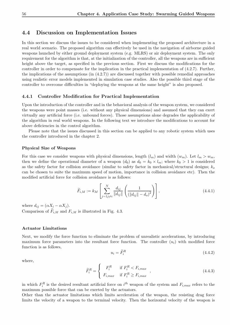
56 Chapter 4. Application Case Study: Swarming Guided Weapons
4.4 Discussion on Implementation Issues
In this section we discuss the issues to be considered when implementing the proposed architecture in areal world scenario. The proposed algorithm can effectively be used in the navigation of airborne guidedweapons launched by either ground deployment system (e.g. MLRS) or air deployment system. The onlyrequirement for the algorithm is that, at the initialization of the controller, all the weapons are in sufficientheight above the target, as specified in the previous section. First we discuss the modifications for thecontroller in order to compensate for the implication in the practical implementation of (4.2.7). Further,the implications of the assumptions (in (4.2.7)) are discussed together with possible remedial approachesusing realistic error models implemented in simulation case studies. Also the possible third stage of thecontroller to overcome difficulties in “deploying the weapons at the same height” is also proposed.
4.4.1 Controller Modification for Practical Implementation
Upon the introduction of the controller and in the behavioral analysis of the weapon system, we consideredthe weapons were point masses (i.e. without any physical dimensions) and assumed that they can exertvirtually any artificial force (i.e. unbound forces). Those assumptions alone degrades the applicability ofthe algorithm in real world weapons. In the following text we introduce the modifications to account forabove deficiencies in the control algorithm.
Please note that the issues discussed in this section can be applied to any robotic system which usesthe controller introduced in the chapter 2.
Physical Size of Weapons
For this case we consider weapons with physical dimensions, length (lm) and width (wm). Let lm > wm,then we define the operational diameter of a weapon (d0) as d0 = k0 × lm; where k0 > 1 is consideredas the safety factor for collision avoidance (similar to safety factor in mechanical/structural designs; ko
can be chosen to suite the maximum speed of motion, importance in collision avoidance etc). Then themodified artificial force for collision avoidance is as follows:
Fi,M := kM
⎡⎣ N∑j=1j �=i
dij
‖dij‖
(1
(‖dij‖ − do)2
)⎤⎦ , (4.4.1)
where dij = (αXi − αXj).Comparison of Fi,M and Fi,M is illustrated in Fig. 4.3.
Actuator Limitations
Next, we modify the force function to eliminate the problem of unrealistic accelerations, by introducingmaximum force parameters into the resultant force function. The controller (ui) with modified forcefunction is as follows,
ui = FRi (4.4.2)
where,
FRi =
⎧⎨⎩ FRi if FR
i < Fi,max
Fi,max if FRi ≥ Fi,max
, (4.4.3)
in which FRi is the desired resultant artificial force on ith weapon of the system and Fi,max refers to the
maximum possible force that can be exerted by the actuators.Other than the actuator limitations which limits acceleration of the weapon, the resisting drag forcelimits the velocity of a weapon to the terminal velocity. Then the horizontal velocity of the weapon is

Chapter 4. Application Case Study: Swarming Guided Weapons 57
0 2 4 6 8 10−5
−4
−3
−2
−1
0
1
2
3
4
5
For
ce M
agni
tude
Distance from weapon [m]
Fi,M
Modified Fi,M
Operational diameter (d0)
Physical size of a weapon
(a)
w m
lm
d0
dij
(b)
Figure 4.3: Effect of physical size of weapons on the collision avoidance force. Here the operationaldiameter (d0) is selected as 2m. Note that the modified function increases the repulsion force from theneighboring weapon, when the center of the weapon comes closer to the 2m limit. The sub figure (b)represents a real world example describing the scenario, where the robots / agents are represented by cartype vehicles
determined by,
md2(zi)dt2
+ρAr,hCd,h
2‖zi‖2 zi
‖zi‖ = FRi (4.4.4)
where Ar,h and Cd,h represents reference area and drag coefficient for horizontal motion respectively.
Chattering Effect
The nature of artificial forces in stage two of the controller (which is similar to the controller in [138])may cause potential chattering problem. (see Figure 4.4 for behavior of the forces). That is, when thecontroller is in the second stage, if a weapon moves out of the contour, the magnitude of the attractionforce may not be sufficient to attract that weapon into the shape when large number of weapons arealready staying inside the contour. This problem can successfully be eliminated by modifying the Fi,A2
force as expressed in (4.4.5). In the modified function, an additional term is included which increasesthe attraction force when the weapon is staying closer to the contour. Also this addition improves theuniformity of the “Artificial Formation Forces” in either side of the contour.
Fi,A2 := (1 − n(γ, αXi))(kA2
∫γ(z − αXi) ‖dz‖ +
kAC
∫γ
[(z − αXi)‖z − αXi‖3
]‖dz‖
)(4.4.5)
In the above expression kAC is the weighing parameter of the force component which dominates when theweapon is closer to the contour.Alternatively, the condition provided in Proposition 4.3.3 can be used to define “X Weapon System”
parameters and to select a kA2 parameter which ensure cohesiveness of the weapons under Fi,A2 force.

58 Chapter 4. Application Case Study: Swarming Guided Weapons
0 200 400 600 800 10000
500
1000
1500
2000
2500
3000
3500
4000
4500
5000
Distance From Center [m]
For
ce [N
]
Fi,R2
Fi,A2
Modified Fi,A2
Figure 4.4: Behavior of stage two “Artificial Formation Forces” at the contour boundary.For better visualization of the changes in forces, the Fi,R2 & Fi,A2(modified) forces are limited up to 5000N .
4.4.2 Implementation, Technologies and Error Models
The proposed algorithm for controlling a weapon system has two basic implementation steps; initialparameter selection (design) and deployment. Prior to the deployment, the target contours are to beclearly defined and the corresponding contour functions relative to the weapon coordinate system (e.g.GPS) are to be generated. Considering the weighing parameters of the artificial force functions (i.e.kM , kF , kA1.. etc.), the proper parameters have to be selected depending on the application and theconstrains provided in the analysis sections. The next step is to deploy the weapons programmed withdesigned contours and group parameters. Also the algorithm provide provisions to change the contourfunctions and parameters to add/remove weapons in an already deployed system. But this needs effectivecommunication between control center (base station) and the group. The behavior of the weapons in suchsituations are presented in the simulation section.
Remark 4.4.1. In the pre-deployment stage, the targets can effectively be identified using satellite maps.Also real-time satellite coverage and aerial video updates from UAV’s can be used to determine theshape/location changes in the target contour (specially when the target is moving), for dynamic parametermodifications of the weapon system.
4.4.3 Obstacle Avoidance
This is one of the most important aspects in real world implementation of the algorithm (see [141, 142,143, 144]). Here we assume that the obstacle is previously identified and can be defined by a simple closedcontour in the 2D plane. Then the artificial force acting on ith member from the obstacle O is as follows;
Fi,O := kO
∫γO
[(αXi − zO)‖αXi − zO‖4
]‖dzo‖ , (4.4.6)
where kO is a weighing parameter determining the magnitude of the force. Terms γO ∈ C and zO ∈ C arethe contour (simple closed) defining the shape of the obstacle and a point on that contour respectively.
Remark 4.4.2. In defining the above artificial force for obstacle avoidance, we used1
‖zi − zo‖3 as the
magnitude of the force from each point, which enables the swarm to navigate closer to the obstacleboundary when deviating from the path. This form of a force function is specially useful for obstacleslocated closer to the target contours, such that the repulsion force from the obstacle do not prevent agentsfrom converging into the shape. Also this definition allows us to include obstacles inside the target contourenabling the agents to acquire complex shapes.

Chapter 4. Application Case Study: Swarming Guided Weapons 59
−1000 −500 0 500 1000 1500
−1500
−1000
−500
0
500
X−Coordinate [m]
Y−
Coo
rdin
ate
[m]
Initial positions @t=0
Final positions@t=1000
(a)
0 200 400 600 800 1000 1200 1400 1600
−1800
−1600
−1400
−1200
−1000
−800
−600
X−Coordinate [m]
Y−
Coo
rdin
ate
[m]
(b)
Figure 4.5: Motion of the swarm in presence obstacles
Contour a b c dFigure(a)-Target 5 1 0.5 80Figure(a)-Obstacle1 3 1 0.0 30Figure(a)-Obstacle2 4 1 0.0 70Figure(a)-Target 5 1 0.5 50Figure(a)-Obstacle1 3 1 0.0 30Figure(a)-Obstacle2 4 1 0.5 20Figure(a)-Obstacle3 4 1 0.2 20
Table 4.1: Parameters used in shape generation
We present two simulation case studies to demonstrate the behavior of the swarm in the presenceof obstacles. In the first case (Figure 4.5.(a)) the vehicles (mobile robots) are in a line formation (forexample along a road or in a convoy) and the target contour is located beyond two obstacle contours. Asillustrated in the figure, the mobile robots successfully avoid both obstacles and form the desired shapeby t = 1000s. In the second case, we consider a situation where mobile robots are randomly distributedaround the target contour. Here we used two obstacles outside the target contour and one obstacle insidethe target. Here also the mobile robots successfully maneuvered around the obstacles and moved into thedesired shape. (The parameters listed in table 4.1 are used for this simulation case.)

60 Chapter 4. Application Case Study: Swarming Guided Weapons
Case ka kr km
case (a) 5 × 10⁻³ 5 × 10³ 7 × 10⁵
case (b) 5 × 10⁻³ 5 × 10³ 5 × 10⁵
Table 4.2: Weighing parameters for artificial forces
Figure 4.6: Robots navigate using restricted inter-member force due to limited communication range.
Localization and communication issues
For successful implementation of the algorithm, the ideal weapons need the following capabilities;(i). Instantaneous and error free self localization.(ii). Knowledge of location of all other members of the group without delay (using communicationnetwork)Here we discuss the practical implementation issues and some technologies which provide near idealcapabilities to the weapons.Since our weapons system is supposed to have GPS/INS navigation system which eliminate short rangeinaccuracies of GPS other than the random error of localization, the localization error can be modeled asfollows;
zi = zi + ηi (4.4.7)
where zi is the actual position and ηi refers to the random noise (σηi = GPS error and μηi = 0).
In the shape formation algorithm, knowledge of position of all the weapons is important in determiningthe collision avoidance force (Fi,M ). This location information is sent through a wireless RF links (orcommunication network). However, the ability to communicate with each other at the same time canbe restrictive in real world applications. Even if CDMA2 technology [145] was used to communicatewith many devices at once, due to high degree of interferences, the effectiveness of the communicationwill degrade with increasing number of weapons in the group. The interferences can be minimized usingtransmission power control, although it reduces the range of transmission. Wireless mesh networkingtechnology ([146, 147]) can be a better solution since it enables handling large data flows within largenumber of nodes [148]. Delays in data transmission (via routing) and range limitations [149] are somedrawbacks in the wireless mesh networking. However the effect of range limitations will not appearin communication within the weapon system. This is due to the obstacle free environment in upperatmosphere where the weapons operate.
Although near ideal wireless communications within the group can be achieved, the problem of elec-tronic and radio jammers in military operations will degrade the communication capabilities significantly.This arise the need of secondary (backup) method of collision avoidance (such as sonar/laser range andbearing estimation) which can locate at least the neighboring weapons. Thus the collision avoidance force
2CDMA (Code Division Multiple Access) technology enables simultaneous access of the whole frequency spectrum withouttime divisions, increasing the number of wireless nodes connected to a single station in an instance.

Chapter 4. Application Case Study: Swarming Guided Weapons 61
Earth Surface
Range of the jammer
Altitude for "Freezing" the relative motion
Stage Switching altitude
Altitude bracket of weapon release
Targetarea
Travel height in the "cohesive" stage
Figure 4.7: Communication jammer range and altitudes of operation
function model for a weapon system with communication failures (limitations) can be given as follows;
Fi,m := km
⎡⎣ N∑j=1j �=i
dij
‖dij‖
(1
(‖dij‖ − do)2
)⎤⎦ ,∀j (4.4.8)
where ‖dij‖ < dc.Here dc refers to the radius around a weapon in which the neighboring weapons can be successfully located.For successful operation of the weapon collision avoidance force, a rough relative location estimate issufficient. However the stage switching requires the position information of all the weapons in the system,thus communication jammers can effectively degrade the performance of stage switching. Generally theeffective range of communication jammers are limited to a certain radius from the physical location ofthe jammer. Thus the above problem can be eliminated by selecting a release height for weapons whichensure that the weapons are switched to the second stage (see section 4.3.2 for vertical distance traveledin the cohesive stage) when reaching the effective radius of the jammer (see figure 4.7).
Upon the introduction of the controller we have made a restrictive assumption such that all theweapons are at the same height at the initialization of the algorithm. This means that the weaponsin the system do not have relative altitude differences. However in a real-world battle field environmentspecially for weapon deployments performed by different air crafts, it may not be always possible to satisfythe above altitude criteria. This results in weapons operating in different altitudes. In such instances,the weapons released at lower heights will reach the target first (since we do not control the verticalmotion of the weapons), triggering a loss of weapons event (see simulation for a demonstration of loss ofweapons event). This causes redistribution of remaining weapons which is not intended. Above problemcan be easily eliminated by introducing another stage to the controller, which “freezes” the positions ofthe weapons (relative to each other) once the first weapon reaches a certain altitude bracket. Moreover,defining the “freezing” altitude higher than the range of the jammers (see figure 4.7) will enable stableweapon control in the presence of radio/electronic jammers.
Computational Issues
The path generation in the proposed weapon system is a real-time and a decentralized process. Thatis each weapon calculates its own path (next position) based on the desired contour information, selflocation (state) information and the position information of other weapons in the system. This is acontinuous process and the frequency of the path calculation (sampling rate) determine the navigationalaccuracy of the weapon system. Since the path planning needs computation of artificial forces consistingof line integrals, a significant computational burden is imposed on the weapon control electronics. In thenumerical evaluation of line integrals, the resolution of the contour define the accuracy as well as thetime required for the calculation. There is a trade-off between accuracy and speed of the line integralcalculation and hence the user must carefully select the resolution of the contour which best suits aparticular application.

62 Chapter 4. Application Case Study: Swarming Guided Weapons
AB
C
D
E
Target Area
Figure 4.8: Defining multiple weapon densities in a single target area. Green circles represent the circleswith radius rc which are used for stage switching at corresponding target area
Shape Generation and Uneven Weapon Distribution
Populating the weapons into a pre-defined ground target needs careful selection of the target contourwhich satisfy the “simple/closed” criteria as well as enclosing the complete target. Note that at theintroduction of the controller, the target contour was defined as a mathematical function in the complexdomain. In reality, due to the complex geometries of the target area, defining the target shapes as amathematical function is not always possible. Moreover, the numerical computation of path planningrequires the target contour as a set of coordinates. Such point based contour generation enables the userto define any odd shaped contour which covers the target area (see the simulation results in figure 4.13for a weapon system assigned to a target generated as a series of points).Another major concern in military operations is the density of weapon distribution, i.e. some sections ofthe target area needs more explosives than the rest of the target. For example in figure 4.8, the section“A” in the target area needs higher density of weapons than the remaining sections of the target. Toachieve this non-uniform weapon distribution, the original target area can be divided into several targetsas illustrated in the figure 4.8 and assign the required number of weapons to each target sector as required(see the simulation results in figure 4.11 and 4.12 for the behavior of the weapon system assigned to twodifferent target areas).
4.5 Simulation Results
The guided weapon system is simulated for three basic cases, (i) releases height, convergence and for-mation behavior analysis for ideal conditions, (ii) evaluating the validity of the release height calculationand demonstrating the performance of algorithm for a real world scenario, (iii) and to demonstrate thebehavior of the second stage controller in disturbances (shape transition, removal/addition of members).To compare the performance of the real and ideal situations, we present the simulated events for first twocases together.
First we demonstrate the behavior of the weapon system released by multiple aircrafts and converginginto a single target area. For the second event, we selected a situation where weapons launched from asingle deployment system moving toward two targets. In both events the released height was calculatedtheoretically and compared with simulated (both ideal and real scenarios) vertical travel when all themembers converge into the circle. For the behavior demonstration under the second stage controller, wepresent only the motion of the weapons in horizontal directions.
In the simulation case studies (except the point generated shape), the shape contours are generated bythe mathematical function described in Appendix I. Also the artificial friction force weighing parameteris selected by kF = 2
√mkA1l(γ) + 1, which enables stable convergence of the whole swarm toward the
contour. The mass of the robot (m) is kept constant at 100kg and density of air ρ is considered to be

Chapter 4. Application Case Study: Swarming Guided Weapons 63
−2000−1000
01000
2000
−2000−1000
01000
20003000
0
1000
2000
3000
4000
Y−Coordinate [m]
X−Coordinate [m]
Hei
ght [
m]
500 1000 15001200
1400
1600
1800
2000
2200
2400
2600
2800
X−Coordinate [m]
Y−
Coo
rdin
ate
[m]
(a) 3-D view of the motion (b) Aerial view of the motion
Figure 4.9: Motion of Weapon System Aimed at a Single Target - Ideal Conditions
constant at 1.814kg/m3 for every simulation case. Further, in all simulations the parameters determiningthe vertical drag force are as follows; Cd = 0.4, Ar = 1.57m2. Moreover, in the realistic simulated caseswe use following parameters, Cd,h = 0.1, Ar,h = 0.53m2, a random localization error of 5m (i.e. σ(ηi) = 5,μ = 0) and acceleration is limited to 2G (19m/s2).
Remark 4.5.1. In figures 4.9, 4.10, 4.11, 4.12, 4.13 the red dots represents the position of each weaponwhen the system switched to the second stage of the controller. The black dots represents the positionsof each weapon when reached the target shape (i.e. when contact the target area) while crosses representthe initial positions of the weapons.
4.5.1 Multiple Aircrafts Engaged in a Single Target
Here all the weapons are released at 4500m altitude. Considering the target is at 0m altitude, thecalculated minimum altitude weapon release is 3167m. In the simulation case studies, the weapons inideal conditions (Figure 4.9) converged to the desired radius after traveling 757m in vertical directionand in under realistic conditions (Figure 4.10) it takes up to 1584m of vertical travel, which is well belowthe calculated travel height. Also under the ideal conditions, the weapon system took 2798m for allthe weapons to achieve less than 2m/s horizontal speeds and under realistic conditions it took 4289mof vertical travel. In selecting the 2m/s speed limit, based on extensive simulation case studies authorsnoticed that the motion of the weapons with less than 2m/s does not contribute in spreading insidethe shape significantly. The following parameters were used in the simulations, kA1 = 0.0025, kA2 =0.01, kR2 = 1 × 10⁵, kM = 6 × 10⁶, a = 3, b = 1, c = 0.5, d = 300 and N = 34.
4.5.2 Single Aircraft Engaged in Multiple Targets
All the weapons are released at 4500m altitude. Considering the target is at 0m altitude, the calculatedminimum altitude weapon release is 3304m. In the simulation case studies, the weapons in ideal conditions(Figure 4.11) converged to the desired radius after traveling 1055m in vertical direction and in underrealistic conditions (Figure 4.12) it takes up to 2183m of vertical travel, which is well below the calculatedtravel height. Also under the ideal conditions, the weapon system took 3180m for all the weapons toachieve less than 2m/s horizontal speeds and under realistic conditions it took 3467m of vertical travelThe parameters used in the simulations are shown in table 4.5.2, while kM is selected as 6 × 10⁶. In thesimulations 34 weapons were directed to shape 1 and 20 were directed to the shape 2.
Remark 4.5.2. In above cases, the vertical distances traveled by the weapon system to “fully spread”inside the given contour under ideal conditions are less than the corresponding calculated released height

64 Chapter 4. Application Case Study: Swarming Guided Weapons
−2000−10000
10002000
−2000
0
2000
0
1000
2000
3000
4000
Y−Coordinate [m]X−Coordinate [m]
Hei
ght [
m]
500 1000 15001200
1400
1600
1800
2000
2200
2400
2600
2800
X−Coordinate [m]
Y−
Coo
rdin
ate
[m]
(a) 3-D view of the motion (b) Aerial view of the motion
Figure 4.10: Motion of Weapon System Aimed at a Single Target - Realworld Conditions
Table 4.3: Parameters used for simulations in Figure 4.11 and 4.12
Shape a b c d kA1 kA2 kR2
1 3 1 0.5 250 0.0025 0.01 2 × 10⁴
2 5 1 0.5 100 0.0005 0.01 2 × 10⁴
−2000
0
2000 −20000
2000
0
1000
2000
3000
4000
5000
Y−Coordinate [m]X−Coordinate [m]
Hei
ght [
m]
−1500
−1000
−500
0
500
1000
1500
1500 2000 2500Y−Coordinate [m]
X−
Coo
rdin
ate
[m]
(a) 3-D view of the motion (b) Aerial view of the motion
Figure 4.11: Motion of Weapon System Aimed at a Multiple Targets - Ideal Conditions
for convergence. Under realistic conditions the vertical distances traveled for achieving the same state areslightly greater than the calculated release heights.
4.5.3 Point Generated Shapes
In real-world military missions, it is not always possible to generate the required target shape by amathematical function. Instead the shape has to be generated by a series of points (i.e. defining coordinatepoints to generate the shape contour). With this method, any arbitrary shape can be generated for the

Chapter 4. Application Case Study: Swarming Guided Weapons 65
−2000
0
2000 −20000
2000
0
1000
2000
3000
4000
5000
Y−Coordinate [m]X−Coordinate [m]
Hei
ght [
m]
−1500
−1000
−500
0
500
1000
1500
1500 2000 2500Y−Coordinate [m]
X−
Coo
rdin
ate
[m]
(a) 3-D view of the motion (b) Aerial view of the motion
Figure 4.12: Motion of Weapon System Aimed at a Multiple Targets - Realworld Conditions
5001000
15002000
−20000
2000
0
1000
2000
3000
4000
5000
6000
7000
8000
9000
Y−Coordinate [m]
X−Coordinate [m
]
Hei
ght [
m]
0 500 1000 1500 2000 25000
500
1000
1500
2000
2500
X−Coordinate [m]
Y−
Coo
rdin
ate
[m]
(a) 3-D view of the motion (b) Aerial view of the motion
Figure 4.13: Motion of the weapon system into a point generated arbitrary shape.
weapon control algorithm. In this case study, we present a formation of 65 weapons into a shape definedusing 234 points (see figure 4.13). Here, the center of the circle for stage switching is located closer to thecenter of the contour and the radius is manually selected to reach the contour line.
4.5.4 Shape Transitions
Here we demonstrate the behavior of the weapon system, when subjected to a sudden change in thecontour’s shape. This kind of shape transitions are important in real world applications, specially whentargeting changing and moving targets, such as convoys, gathering of vehicles etc. From the computersimulation results shown in figure 4.14, the weapon system initially in a heptagonal formation (representedin red) is disturbed by a transition of the contour shape. The figure illustrates the motion paths and finalpositions of the weapon system forming into the new triangular shape. It is clear from this simulation,the weapons effectively maneuver themselves to form the new shape and redistribute within that shape.

66 Chapter 4. Application Case Study: Swarming Guided Weapons
800
1000
1200
−2600
−2400
−2200
−2000
7200
7400
7600
7800
8000
X−Coordinate [m]
Y−Coordinate [m]
Hei
ght [
m]
Figure 4.14: Behavior of the weapons in shape transitions. Initial weapon configuration at 8000m wasdisturbed by shape transition. Weapon positions and shape in red color represents the initial conditionsand the final conditions are represented in black color.
The simulation used the parameters in table 4.4.
Table 4.4: Parameters used to generate Figure 4.14
Case a b c d kA2 kR2 kM
Initial 7 1 1 45 4 × 10⁻³ 5.2 × 10³ 5.9 × 10⁵
Final 3 1 0.8 130 4 × 10⁻³ 5.2 × 10³ 5.9 × 10⁵
4.5.5 Addition/Removal of Agents
Ability to reconfigure the weapon’s horizontal positions, when subjected to addition or removal of weaponsdemonstrate significant importance in achieving effective distribution. In most deployments targetingmilitary establishments, the weapons have high probability in caught up with enemy fire. In such circum-stances, redistribution of remaining weapons to cover the target area is highly advantageous in deliveringeven destruction to the target area. Also, some times inclusion of additional weapons is also a possiblescenario, when the existing number of weapons become insufficient for the target. With this simulationcase study, we present the behavior of the weapon system (operating in second stage of the controller) inremoval (Figure 4.15(a)) and addition (Figure 4.15(b)) of the weapons.
For the simulations we used the parameters listed in table 4.5.
Table 4.5: Parameters used to generate Figure 4.15
Case a b c d kA2 kR2 kM
Addition 6 1 0.5 55 4 × 10⁻³ 6.2 × 10³ 5 × 10⁵
Removal 6 1 0.5 55 4 × 10⁻³ 7 × 10³ 9 × 10⁵

Chapter 4. Application Case Study: Swarming Guided Weapons 67
800
1000
1200
−2500−2400
−2300−2200
−2100
5500
6000
6500
7000
7500
8000
X−Coordinate [m]Y−Coordinate [m]
Hei
ght [
m]
(a) Removal of Members in the Flight
600800
10001200
−2600
−2400
−2200
−2000
5500
6000
6500
7000
7500
8000
Y−Coordinate [m]X−Coordinate [m]
Hei
ght [
m]
(b) Addition of New Members in theFlight
Figure 4.15: Behavior of the Weapon System when disturbed while in Flight. In sub figure (a), theweapons removed from the group at 8000m altitude are represented by red crosses. In sub figure (b)Initial configuration at 8000m was disturbed by new additions to the group. The paths and positions ofnew additions are shown in red color.
4.6 Summary
In this chapter we have presented an approach to control a group of guided weapons to be distributedinside a given geographical shape, specified by either a mathematical function or series of points. Thecontrol algorithm uses artificial formation forces to attract and guide the weapons into the shape. Ar-tificial inter-weapon repulsion forces were used to distribute the weapons evenly inside the shape whileeliminating collisions among weapons. The two tier controller of the proposed weapon system ensuresstable convergence of the weapons into the desired shape. The weapon system was analysed for stability,time of convergence, and conditions for cohesive behavior. Moreover, an important result on the releaseheight of the weapon system was obtained which ensures that all the weapons are converged into thedesired geographical boundary at the time of impact. Computer simulations were used to verify thetheoretical assertions and the behavior of the weapons when subjected to sudden change of target shape,loss/addition of weapons into the group etc. Also a modified model compensating for the size of weapons,thrust limitations and errors in localization which closely resemble real-world scenarios, was introducedand computer simulations were used to confirm the behavior.


Chapter 5
Communication and Power SavingSchemes for the Swarm
Swarm robotics and wireless sensor networks, can sometimes be considered as a single research discipline.In many cases, the algorithms developed for ad-hoc connected wireless sensor networks can be directlyused for communications in swarm robotics, which share similarities such as limited relative mobility,ad-hoc connectivity, utilization of limited energy reserves, small data packet size, fast communicationetc,. In this chapter we introduce two communication protocols that are specifically designed to save thelimited energy reserves in energy critical wireless communication links while achieving the goal of effectivecommunication. The communication algorithms introduced in this chapter are primarily focused on wire-less sensor networks domain, however they can be adopted in multiple robot coordination domain withoutany modifications. The concluding chapter (chapter 6) of this dissertation illustrates such scenario.
In the robotic swarm introduced in this dissertation, the knowledge of the positions of the othermembers is critical for accurate pattern generation. Specially in the two-stage controller introduced inthe chapter 4, the instantaneous knowledge of the other members of the swarm is utmost important inswitching to the second stage of the controller. In the section 5.1, we introduce an all-to-all communi-cation algorithm to be used for communication within the swarm. The proposed architecture satisfiesthe instantaneous knowledge of positions of every member in the swarm as well as uses the minimumtransmission power to convey the message.
In the section 5.2 we introduce an algorithm for controlling the transmission powers of remote wirelessagents deployed in a mobile data collector based data gathering scenario, which has many potentialapplications in the swarm robotic domain.
5.1 Fully-Connected mesh network for effective communication
1Recent past has witnessed a growing popularity in the multi-cast networking technologies, which haveadded advantages in the modern communication needs such as internet based multimedia services (news,distant learning etc), multimedia conferencing facilities for computers and mobile phones[150, 151].
In multi-casting, the broadcasting of a single data packet to the network by the node dramaticallyimproves the bandwidth usage in comparison to the unicast networks (one-to-one networks). In additionto the multimedia communication; distributed computing, parallel processing , swarm robotics , andwireless sensor networks where each node have some information to share with the other nodes havedistinct advantages in employing all-to-all networks (multi-casting) [152].
All-to-all communications, proposed by Yang and Wang can be classified as: all-to-all broadcastingand all-to-all personalized exchange depending on the nature of the communication[153]. In the formercase, the information (data packet) originating from a single node is propagated through the entire
1Please note that the material presented in this section is based on the conference paper: S.W. Ekanayake, P. N. Pathirana,B. F. Rolfe, and M. Palanaswami, “Energy efficient, fully-connected mesh networks for high speed applications,” in IEEEVehicular Technology Conference, VTC2008, Singapore, 2008
69

70 Chapter 5. Communication and Power Saving Schemes ...
network and in the latter case every node has distinct information to share with every other node inthe network. Routing algorithms for both network types have been extensively researched in the past[154, 155, 156, 157, 158]. However, these routing algorithms were based on multi-hopping mesh andtorus based network architectures and involve routing tree generation, forwarding link assignments, sub-network creation etc. They also have many practical difficulties in applying to all-to-all ad-hoc networks[159, 160, 161]. In modern distributed / parallel processing applications, the network essentially consistsof time varying nodes (location changes and addition / removal of nodes), which cause changes in themesh / torus at each instance of architectural change. Moreover, those multi-hopping all-to-all networkscomprises of hopping (routing) delays and increased network congestion with increasing network traffic,resulting in loss of vital information.
In this section, we consider a situation where an ad-hoc connected multiple-node wireless networkrequiring instantaneous all-to-all personalized communication, which is distributed within a close rangesuch that the single-hop communication can be achieved between every node. The communication schemeintroduced here enables all-to-all networking of the nodes without forwarding tree generation based onthe spatial configuration of the nodes, i.e. node mobility, addition / removal of nodes etc. The proposednetwork uses CDMA based communication architecture which enables the entire network to communicatesimultaneously. Moreover, we derive the capacity of the network in-terms of the number of nodes in thenetwork and introduce a power control algorithm which ensures that all the nodes are transmitting at theminimum possible transmission power while maintaining the connectivity of the entire network ensuringinterference free communication.
The rest of this section is organized as follows. In the sub-section 5.1.1, we discuss the relatedwork in the CDMA power control and power control aspects in ad-hoc networks. Then in the problemformulation (sub-section 5.1.2), we introduce the network architecture and the communication model usedin this research. Furthermore, we derive the capacity of the network for QoS guaranteed communicationlinks based on the CIR constraint. Then the Power Control (PC) algorithm is introduced and the controlparameters are analyzed in the sub-section 5.1.3. Also we use computer simulations to illustrate thebehavior of the system operating under both ideal and real-world conditions.
5.1.1 Power Control in Wireless Networks
CDMA and Power Control in Cellular Systems
Among the multiple access schemes in wireless communications, CDMA has become the most promisingtechnology that can satisfy most aspects in modern communication networks, such as higher speeds, largerclient base and QoS guaranteed communication. Although CDMA started service in cellular communi-cations in late 90’s, the concept was originally introduced by Claude Shannon and Robert Pierce in 1949[162], and then extended by DeRosa-Rogoff, Price & Green and Magnuiki [163, 164]. The early devel-opments of this technology were primarily focused on the military and navigation applications (satellitecommunication etc). As the first civilian application, a narrow-band spread spectrum CDMA scheme forcellular communication was first proposed by Cooper and Nettleton in 1978 [165] and then developed tothe IS-95 and CDMA2000 standards which are used in modern CDMA wireless communications [166].
Maintaining the Carrier-to-Interference Ratio (CIR), alternatively referred as the co-channel interfer-ence, at a desirable level is the main aspect of power control in CDMA networks. In CIR balancing, thetransmission powers of every user device is controlled such that it ensures the co-channel interference ofeach link guarantees QoS reception. CIR balancing in a cellular system has two aspects: intra-cell CIRbalancing and inter-cell CIR balancing. In intra-cell CIR balancing the user devices control the trans-mission power such that it provides a constant received power at the base station [167] to avoid near-farproblem. This method is currently in practice with CDMA standards such as IS-95 and CDMA 2000[145]. Inter-cell CIR balancing received widespread attention among the academic community after theproblem reformulation by Zander et al. in [168]. This work was further investigated by Grandhi et al.[169, 170, 171] and the Distributed Power Control (DPC) scheme proposed by Foschini and Miljanic [172]has become a standard benchmark due to its academic and practical significance (see [173, 174, 175] for

Chapter 5. Communication and Power Saving Schemes ... 71
ith Node
Gij
jth Nodekth NodeGkj
Figure 5.1: An all-to-all network consisting of six nodes.
further improvements), which was later adopted into wireless communication standards [176].
Power Control Aspects in Ad-hoc Networks
Many wireless ad-hoc networks, such as sensor networks and military communication networks, are inher-ently associated with restrictions in power consumption mainly due to the limited energy resources suchas batteries. Therefore, unlike in cellular communications, the power control in wireless ad-hoc networksare basically focused on energy conservation. Many power conservation techniques introduced for suchnetworks can be found in the past research literature[177, 178, 179, 180, 181, 182, 183, 184]. Among themrouting optimization [177, 178, 179, 180] and transmission power control [181, 182, 183] are the widelyresearched areas. However as opposed to the above, different effective methods such as sleep and wakeupprocedures implemented in the hardware layer [184], were also proposed.
5.1.2 Problem Formulation
Now we formally introduce the power control problem together with the associated network architecture,control constraints and network capacity.
Network Architecture
Consider a single hop all-to-all wireless network (Ω) in which N nodes communicate with each othersimultaneously (see Figure 5.1) using spread-spectrum multiple access protocol (such as CDMA). Inthis network, the nodes are broadcasting the data continuously, rather than maintaining node-to-nodecommunication links. The broadcast data from a particular node, which is uniquely coded, can be accessedby every other node in the network.
The network model assumes followings;
• Nodes have instantaneous and error free Received Signal Strength (RSS) measurement capabilities.
• The measurements are immediately included in to the broadcast data, which will be used for thePC process.
• Link gain variations are negligible compared with the communication and the data processing time.
• All the nodes in the network are identical in performance (homogeneous).
In the controller analysis, the above assumptions are used in order to reduce the system complexity;however in later sections we relax these assumptions and present the controller behavior with erroneousmeasurements, non-homogeneous node properties, and link gain variations which resemble a real-worldscenario.

72 Chapter 5. Communication and Power Saving Schemes ...
Control Constraints
In order to achieve QoS guaranteed communication in every link, two conditions must be satisfied simul-taneously; CIR constraint and the connectivity constraint.
CIR Constraint : Any node j in the network can receive the signal transmitted from any othernode i, correctly, if the CIR measured at the jth node (γij) is greater than the threshold CIR value γt.Then the CIR constraint can be defined as;
γij =PiGij
N∑k �=i,k �=j
PkGkj + η
≥ γt, ∀i, k, j ∈ Ω (5.1.1)
where Pi is the transmission power levels of the ith node. In the above expression, Gij and Gkj are thelink gains between i, j and k, j nodes respectively. Here the η represents the noise power (thermal noise)in the communication link and this is assumed to be constant for the geographical area (see [173, 172]).
Connectivity Constraint : To receive a signal from any node i, the received power level of thesignal measured at the jth node (Rij) must be greater than the receiver threshold Rmin, which is thesensitivity of the receiver hardware. In this study the threshold received power is defined such that, thereception is not affected by the thermal noise of the band. Then the received power condition can bedefined as (considering Rij = PiGij + η);
PiGij + η ≥ Rmin, ∀i, , j ∈ Ω . (5.1.2)
Capacity and spatial limitations
In order to satisfy the above constraints, the all-to-all network has certain limitations in the spatial con-figuration and network capacity. This section derives the network capacity which ensure QoS guaranteedcommunication, and the relationships between the receiver sensitivity and the spatial configuration (linkgains) to maintain reliable links.
From the connectivity constraint we get,
mini,j∈Ω
(PiGij + η) ≥ Rmin, (5.1.3)
which provides a condition that the network should satisfy at all the times for the power control algo-rithm to perform the desired action. Moreover, the network always satisfies the connectivity constraint(“connectivity guaranteed” networks) if:
PminGmin ≥ Rmin − η; (5.1.4)
and the network is “feasible” if:PmaxGmin ≥ Rmin − η. (5.1.5)
Here, Pmin and Pmax refers to the minimum and maximum transmission power levels of the nodes re-spectively, and Gmin is the minimum link gain between any two nodes in the network. Above, the term“feasible” means that the network can achieve the connectivity constraint.
From the CIR constraint (equation (5.1.1));
mini,j∈Ω
(PiGij)(
1 + γt
γt
)≥ max
k,j∈Ω
⎛⎝ N∑k �=j
PkGkj + η
⎞⎠ , (5.1.6)
thus for “connectivity guaranteed” network:
PminGmin
(1 + γt
γt
)≥ (N − 1)PmaxGmax + η,

Chapter 5. Communication and Power Saving Schemes ... 73
resulting,
N ≤ 1 +(
1 + γt
γt
)(PminGmin
PmaxGmax
)−(
η
PmaxGmax
). (5.1.7)
For the “feasible” network:
PmaxGmin
(1 + γt
γt
)≥ (N − 1)PmaxGmax + η,
limiting the capacity as,
N ≤ 1 +(
1 + γt
γt
)(Gmin
Gmax
)−(
η
PmaxGmax
). (5.1.8)
Definition 5.1.1. Limited Capacity Network : A multi-casting network satisfying the equation (5.1.8)on the number of nodes is defined as a Limited Capacity Network.
Remark 5.1.1. In above derivations, the network capacity is determined in terms of the number of nodesconnected (N) at an instance and this number is dependent on the target CIR (γt). In spread spectrumnetworks, γt is selected to maintain the desired network quality, bandwidth and the data transfer speed[167]. Thus limiting the number of nodes to N ensures that the desired communication capacities/qualitiesare preserved in the network.
Remark 5.1.2. In limited capacity networks, the range of link gains in the desired geographical area(Gij ∈ [Gmin, Gmax]) is a decisive factor on the number of nodes. However, this enables us to accuratelyselect the number of nodes to be deployed in a particular region, knowing the range of link gain at thatregion.
Remark 5.1.3. In limited capacity networks, the maximum number of nodes (Nmax) is defined such thatthe networks always satisfy the CIR constraints without directly depending on the spatial distribution ofthe nodes. However, this does not mean that a network with number of nodes N > Nmax in the samegeographical area (not necessarily in the same configuration) does not satisfy the CIR constraints.
Intended Controller Behavior for Energy Conservation
In this power control problem, we consider an ad-hoc network satisfying “Limited Capacity” and “feasible”conditions. The problem considered here is to maintain all-to-all communication links in such networks,while minimizing the network power consumption via transmission power control. The proposed powercontrol algorithm is focused on maintaining minimum requirements for satisfying the connectivity con-straints, which automatically satisfies the CIR constraint in a Limited Capacity network.
5.1.3 Iterative Controller
In this section, we present a transmission power control scheme (see figure 5.2) to maintain the receivedpowers at the desired value that satisfy the connectivity of the network, and derive the tolerance limit forselecting the target received power.
The transmission power of the ith node (Pi) is determined by,
Pi = a(ei −Rt), (5.1.9)
here a < 0 is a constant, ei is the average received power at the other nodes, i.e ei =
N∑j �=i
(PiGij + η)
N − 1, and
Rt is the target received power which satisfy the connectivity constraint for all the nodes.
Remark 5.1.4. In this power control algorithm, we assume that the nodes are transmitting at the maximumtransmission power at time zero (at the initialization of the algorithm).

74 Chapter 5. Communication and Power Saving Schemes ...
nth Node
ith Node
1st Node
jth Node
(n-1)Rt
a +++ -
Pj(t-1)
Pj(t)
++
++
++
P1(t)
Pi(t)
Pn(t)
Figure 5.2: Block diagram representation of the controller of the jth node
5.1.4 Convergence of the controller
From the definition we have, ei = PiAi + η and thus ei = PiAi, where Ai =
∑Nj �=iGij
N − 1is the “average link
gain” for the ith node.With this, the controller function can be reformulated as:
ei = aAi (ei −Rt) ,
From the above expression it is evident that the control variable ei converges to Rt, if ‖aAi‖ < 1.
Remark 5.1.5. Since Gi,j < 0,∀i, j and selecting ‖a‖ < 1 always satisfies the ‖aAi‖ < 1 condition for theconvergence.
Satisfying Connectivity for Every Node
The convergence of the above controller describes the trajectory of the average received power, however,it does not say anything about the trajectories of the RSS in each link or their connectivity. In thissection, we obtain a relationship between link gains, sensitivity of the receiver hardware and the targetRSS value, which can be used to determine the tolerance limit when selecting Rt. This relationship isformally introduced in the following proposition.
Proposition 5.1.1. In an all-to-all network using the power controller described by (5.1.9) and deployedin a geographical area having link gains within a known range, i.e. Gij ∈ [Gmin, Gmax], the connectivity
constraint is always satisfied if the threshold value for the power controller, Rt ≥ Rm + η(X − 1)X
, where
X = mini,j∈Ω
(Gij
Ai
).
Proof. Let the error between the average RSS and the RSS of the node j,
eij = Rij − ei = Pi (Gij −Ai)
and the time derivative;eij = Pi (Gij −Ai) .

Chapter 5. Communication and Power Saving Schemes ... 75
Then using the control function (5.1.9) we have,
eij = aAi
[eij − (Rt − η)
(Gij
Ai− 1)]
. (5.1.10)
Above expression implies that eij converges toward (Rt − η)(Gij
Ai− 1)
, if the conditions for the con-
vergence of ei are satisfied. Since the above statement is valid for any node i, j in the network, we candetermine the lower bound of eij as;
mini,j∈Ω
(eij) ≤ (Rt − η)(
mini,j∈Ω
(Gij
Ai
)− 1). (5.1.11)
For an all-to-all ad-hoc network deployed in the geographical area with Gij ∈ [Gmin, Gmax], we have;
mini,j∈Ω
(Gij
Ai
)=
(N − 1)Gmin
Gmin + (N − 2)Gmax. (5.1.12)
Then, the connectivity condition for any link i, j is satisfied if,
Rt + mini,j∈Ω
(eij) ≥ Rmin,
i.e.
Rt ≥ Rm + η(X − 1)X
(5.1.13)
where,
X = mini,j∈Ω
(Gij
Ai
)which proves the assertion.
Simulation Results
Power control algorithm : In this section a simulation case study is presented which illustrates thebehavior of the system in an ideal situation described in the problem formulation section. The followingparameters were selected for the simulation, Pi ∈ [0.1, 3], Gij ∈ [0.3, 0.6], Rmin = 0.1, γmin = 0.1, η =0.05, and N = 4.With the selected parameters, the feasible condition (Rmin ≤ 0.3 × 3 = 0.9) and the “Limited Capacity”
network condition(N ≤ 1 +
(1.10.1
)(0.30.6
)− 0.05
0.6= 6.417
)are satisfied. The target received power (Rt)
is selected using equation (13) as: Rt = 0.2 >0.1 + 0.05(0.6 − 1)
0.6= 0.1333. The simulation results are
shown in Figure 5.3. It is evident from the simulation figures that the controller converges to the minimumtransmission power that satisfies all the constraints described in the previous section.
Network limitations : In this section we evaluate the theoretical assertions on the networklimitations. In figure 5.4, the variation of CIR with increasing number of nodes is presented. In thisfigure, minimum and maximum CIR values for each node count are obtained by executing the simulationfor 20 times with random selection of gain matrix ,Gij ∈ [0.3, 0.6] and all other values are kept as in theprevious case. It can be seen that the CIR range drops below the threshold value of 0.1 just after thenode count exceeds 7 (the calculated maximum node count N < 6.417).
Controller behavior in a real-world scenario : In this section, we illustrate the behavior ofthe proposed control scheme in the presence of real-world communication properties. Here the network isconsidered to have hertogeneous nodes, erroneous measurements and link gain variations (due to motionand other mobile obstacles).

76 Chapter 5. Communication and Power Saving Schemes ...
0 10 20 30 40 500
0.5
1
1.5
2
2.5
3
Time Step
Tra
nsm
issi
on p
ower
of n
odes
(a) Transmitted Powers
5 10 15 20 25 30 35 40 45 500
0.1
0.2
0.3
0.4
0.5
0.6
0.7
Time Step
CIR
at e
ach
node
γt
(b) CIR of each link
5 10 15 20 25 30 35 40 45 500
0.2
0.4
0.6
0.8
1
1.2
1.4
1.6
Time Step
RS
S a
t eac
h no
de
Rt
Rmin
(c) RSSI of each link
Figure 5.3: Effect of the transmission power control algorithm
The measurement error at jth node is modeled as a normal distribution νj ∈ [0, σ2ν ], and the link gain
is modelled as Gij = Gij10(X/10), where X is the dB attenuation due to shadowing effect and modelled asa Gaussian variable in the form of X N(0, σ2
X ). Then the received power measurement can be modeledas,
Rij =(PiGij + η
)10νj/10. (5.1.14)
The hetrageneous properties are modelled as differences in power transmission and power measurements,which are common in real-world communication equipments. The actual transmission power of the ith
node is modelled as Pi = αiPi, where αi ∈ (αmin, 1) determines the power of the transmitter and is uniqueto each node. Similarly, the received power measurement performance factor βi ∈ (βmin, 1) determinesthe actual measured received power Rij = βiRij .
In the simulation results shown in figure 5.5, we consider σX = 2, σν = 0.4, αmin = 0.8 and βmin = 0.7(αi and βi values are randomly assigned for each node). According to the simulation results, the powercontrol algorithm performs well in the presence of real-world limitations, maintaining the CIR of everylink above the target (threshold CIR) as well as RSS of every link above the minimum RSS.

Chapter 5. Communication and Power Saving Schemes ... 77
2 4 6 8 10 12 14 16 18 200
0.2
0.4
0.6
0.8
1
1.2
Number of Nodes
Min
/Max
CIR
Lev
els
Max CIRMin CIRγt
Figure 5.4: Behavior of CIR with number of nodes in the mesh.
5.2 A simple power control algorithm for mobile data collector basedremote data gathering scenario
5.2.1 Motivation and background
2In most low end networking devices CIR can not be directly measured, instead received power (in dBm)and Link Quality measurements can be obtained directly from the hardware. This raise the need ofpower control algorithms which do not entirely depending on CIR measurements, but depends on rathermeasurable parameters. In this study we derive the optimum value for co-channel interference measuredat a base station, and introduce two power control algorithms to implement in user devices which can alterthe transmission power to obtain the required CIR. In the proposed schemes we make use of ReceivedSignal Strength Indication (RSSI) measurements to achieve the desired CIR at the base station.
In the next section (section 5.2.2) we introduce the problem in a formal manner, and in section 5.2.3we justify our assumptions with experimental reasoning. Then in section 5.2.4 we introduce the controllerand perform analysis for the convergence.
5.2.2 Problem formulation
In this section we introduce the basic assumptions and models which will be used in the power controlscheme. In this study we use the term “Server” to denote the base station node which communicatewith all the “Clients” within the range. Here “Client” refers to the sensory node/ user device which isconnected to the base station. The notation in Table 5.1 is used throughout the paper.Consider a wireless network with n clients connected to a single base station in a typical environment
consisting of uncertainties in RF propagation due to shadowing, multi path propagation etc. The clientscommunicate with the server continuously using a common frequency band (as in CDMA). The server hasa limit of nmax clients connected with it at an instant, and has a receive threshold of Rmin (dBm) which isdepending on the sensitivity of the receiver hardware. Also we assume that the communication networkis not interfered by any other RF network in the domain of the base station (or “cell” in the cellularnetworking terminology). Throughout this paper, we assume that the server and the client maintain acontinuous communication link, in which the server sends an acknowledgment signal back to the clientfor each data packet received (similar to [173]). This signal contains the RSSI of the received packet andthe transmission power (if not transmitting at a fixed power) of the acknowledgment signal, which willbe used in the PC algorithm. Also the communication hardware (server and client) have the capability
2Please note that the material presented in this section is based on the conference paper: S.W. Ekanayake, P. N. Pathirana,andM. Palanaswami, “Maintaining optimal co-channel interference for power efficient wireless communication,” in ISSNIPconference 2007, Melbourne, Australia, 2007

78 Chapter 5. Communication and Power Saving Schemes ...
0 10 20 30 40 500
0.5
1
1.5
2
2.5
3
Time Step
Tra
nsm
issi
on p
ower
of n
odes
(a) Transmitted Powers
5 10 15 20 25 30 35 40 45 500
0.2
0.4
0.6
0.8
1
1.2
1.4
1.6
1.8
Time Step
CIR
at e
ach
node
(b) CIR of each link
5 10 15 20 25 30 35 40 45 500
0.5
1
1.5
2
2.5
3
3.5
Time Step
RS
S a
t eac
h no
de
(c) RSSI of each link
Figure 5.5: Effect of the transmission power control algorithm - Real world scenario
Table 5.1: Notation
P T
i Transmission power of ith node. (dBm)P T
m Transmission power of server node. (dBm)Rm
i Received power measured at client i, transmitted by server node. (dBm)Ri
m Received power measured at server node, transmitted by node i. (dBm)Rm
0 Received power measured at reference distance (d0), transmitted by servernode. (dBm)
Ri0 Received power measured at reference distance (d0), transmitted by client
node i. (dBm)
to measure the RSSI of each data packet.

Chapter 5. Communication and Power Saving Schemes ... 79
Figure 5.6: Modeling of 2D Multi-path propagation inside an enclosed environment, the figure presentsfew possible paths of multi-path propagation.
5.2.3 Path loss model
We use the following path loss models for communication between the client node and the server node,
Rim = Ri
0 − 10η log10
(d
d0
)+ S im (5.2.1)
and
Rmi = Rm
0 − 10η log10
(d
d0
)+ Smi, (5.2.2)
here term η refers to the path attenuation factor, which is a constant depending on the propagation media.In above expressions, Sim and Smi refer to the combined effects due to shadow fading, multi-path propa-gation and any other fading effect occur from environmental factors such as presence of people, animals etc.
For line-of-sight communication in outdoor environments, specially long distance, the propagation ofRF (Radio Frequency) waves can be approximated using free-space path loss model. This is possibleas multi-path propagation and shadow fading effects do not become significant in such environments.Whereas, for wireless networks in indoor environments, the propagation is harder to predict due topresence of multi-path effects. Many researchers have studied the phenomenon of multi path propagationand proposed RSSI models for indoor environments with the presence of obstacles [185, 186, 187, 188, 189].Applicability of those models for mobile nodes is debatable due to dynamic nature of environments andthus the model. Further, the experimental studies done by Lin et. al. in [183] claims that the RSSI valuebetween two nodes in the line of sight have significant changes over the course of the day, thus locationbased mathematical models become inapplicable.Ray-tracing concept for RF propagation, on the other hand, become a handy tool for predicting RSSIvariation in an indoor environment [190, 191, 192]. Here, the radio waves are considered to follow theproperties similar to visual light propagation in the presence of transparent obstacles. The effectivenessof Ray-Tracing method for RF waves increases with high frequencies. This is due to reduced scatteringeffects in shorter wave lengths. We use ray-tracing concept to make an assumption on the Sxx terms inequation (5.2.1) and (5.2.2), as follows;
S im(k) = Smi(k),∀i = 1 . . . n
where k represents a time step in discrete time.As in figure 5.6, there exists more than one path for receiving the signal from a RF source to a sink, and
the overall S term consists combination of all the multi-path propagation terms. With the assumptionabove, we claim that if the sink and source positions in the figure 5.6 was interchanged then the onlydifference with the previous case is that the direction of propagation. That is all the multi-path linksremain the same except the direction, thus results the same S effect at the sink in the new configuration.The following experimental results justifies our assumption.

80 Chapter 5. Communication and Power Saving Schemes ...
Figure 5.7: Experimental setup for the ray tracing experiment - In this figure only four receiver nodesare shown however in the real experiment we used five receiver nodes and performed the experiment inseveral environments representing different disturbance and reflection levels.
Table 5.2: Expected values of measurementsParameter Node 1 Node 2 Node 3 Node 4 Node 5
E(Ri
m
)/ (dBm) -62.56 -65.96 -62.20 -62 -64.01
E (Rmi ) / (dBm) -62.00 -64.00 -61.99 -61.94 -66.00
E(Ri
0
)/ (dBm) -39.28 -40.65 -39.00 -41.00 -37.01
E (Rm0 ) / (dBm) -39.00 -39.00 -38.08 -41.00 -39.00
E (S im − Smi) / (dBm) 0.29 0.31 -0.72 0.06 0.00
Basis for Ray-Tracing Assumption
In this experiment, four nodes (stationary nodes) were placed in an indoor environment and a mobilenode communicating with them was randomly moved in the same environment (see Figure 5.7). Thereceived powers at each stationary node and the received power of the corresponding acknowledgmentsignal at mobile node were recorded. All the nodes are transmitted in a fixed transmission power andthe corresponding Rm
0 and Ri0 values were measured with d0 = 10cm (this was conducted in a large open
space to minimize the effect of multi-path propagation). Then the expected value of the S im − Smi canbe written as follows.
E (S im − Smi) = E(Ri
m
)− E (Rm
i ) + E (Rm0 ) − E
(Ri
0
)The statistical data of the measurements and calculated S im − Smi are presented in Table 5.2.3.

Chapter 5. Communication and Power Saving Schemes ... 81
From the experimental data it is evident that the S im − Smi term is zero. In this experiment, eventhough all the transmitters are transmitting with the same power, we used the measured received powersat a reference distance rather than assuming Rm
0 = Rmi in order to eliminate the effect of antenna gains.
Remark 5.2.1. In environments with such uncertainties (e.g. indoor, urban etc) ray-tracing concept canbe used to predict the radio wave propagation [190, 191]. Here, the radio waves are considered to followthe properties similar to visual light propagation in the presence of transparent obstacles.
5.2.4 Power control analysis
Optimum Carrier-to-Interference Ratio
CDMA base stations have a minimum CIR value (γmin) which guarantee QoS reception. In CIR basedpower control algorithms such as [172, 173, 174] etc the controller is trying to maintain the CIR at afixed value γf ≥ γmin. In this paper, we introduce a dynamic target CIR value (γt ≥ γmin) which is theoptimal CIR for the number of clients connected with the server at that instance. The CIR, measured atthe server, of the communication with the ith client (γi) can be defined as follows,
γi =Ri
n∑j=1,j �=i
Rj
(5.2.3)
where Ri denotes the received power measured at the server, transmitted by the ith client in “Watts”.Note that the Ri includes the random noise of the measurements as well. The server is said to have agood communication with the ith sensor, if the γi is greater than the threshold value γt. Then the abovecan be expressed in the following form (as in [168]),
Rin∑
j=1
Rj −Ri
≥ γt. (5.2.4)
The vector representation of the above is,(1 + γt
γt
)R ≥ 1nR , (5.2.5)
where 1n is the unity matrix and [R]i = Ri. As proposed by Zander in [168] we can derive the optimalγt value as follows (see Remark 1),
γt =1
(n− 1),∀n < nmax, (5.2.6)
which results, Ri = Rt,∀i = 1 . . . n, i.e. the received power values of the signals from every client, mea-sured at the server should be equal. Here Rt is the target received power. This reduces the CIR balancingproblem to a simple power control problem as presented in the next section.
Remark 5.2.2. Using the Perron-Froebenius theorem (see [108]), the largest real eigenvalue of the matrix1n can be found as n.
Remark 5.2.3. Selecting Rt = Rmin results in maintaining the CIR at the optimal value of1
(n− 1)while
gaining the maximum energy saving in the network.

82 Chapter 5. Communication and Power Saving Schemes ...
Transmission Power Control
In this section, we propose a power control scheme to maintain the variable CIR presented in the section5.2.4. Since we proved that maintaining a constant received power at the base station satisfies the optimalCIR condition, the ultimate target of the power control algorithm is to maintain Ri
m at Rt.Iterative Controller
The iterative power control algorithm is proposed as follows;
PT
i = f(Rt − Ri
m
). (5.2.7)
Here the f(·) is defined as any function satisfying the Lipschitz condition,
f(‖a− b‖) ≤ k1‖a− b‖ (5.2.8)
where k1 ∈ [0, 1] is the Lipschitz constant for the function f(·).
Proposition 5.2.1. The controller converges the Rim, starting from any arbitrary value, to Rt, if the
transceiver gains remain constant.
Proof. From the path loss model between the client (5.2.1) and the server (5.2.2) nodes, we have
Rim = P T
i − P T
m + Rmi
and since P T
m is a constant in our problem, the received power at the client node remains a constant.Then the controller becomes,
PT
i = f(Rt − P T
i + P T
m − Rmi
)(5.2.9)
resulting,P
T
i = f(C − P T
i + υi
), (5.2.10)
where C = Rt +P T
m − Rm
i is a constant for the time interval. Here the υi is the random noise in the Rmi ,
i.e. Rm
i = Rmi + υi. Let p =
(C − P T
i
), then p = −P
T
i . The equation (5.2.10) can then be written inthe vector form as,
p = −f(p + υ) = f(−p − υ) (5.2.11)
where [p]i = P T
i , [υ]i = υi and f : �n → �n, i.e. f(a) = [f(a1) . . . f(an)]T ,a = [a1 . . . an]T ∈ �n andf(a) = 0 if a = 0, thus the equilibrium point is the desired transmit power in (5.2.7) giving the optimalCIR in (5.2.6). Then as in [173], selecting a = −pa − υ and b = −pb − υ yields,
‖f(pa) − f(pb)‖ ≤ k1‖(pa − pb)‖. (5.2.12)
Since the above expression satisfies the Lipschitz conditions the system converges toward the desiredpower vector. (see [173] and references there)
The numerical simulation results presented in Figure 5.8 shows the behavior of two controller functions;(1) A linear controller (fL), and (2) A sigmoid based controller (fS), defined as,
fL(a) = 0.3 ∗ a,
fS(a) = 2(−0.5 +
11 + exp(−a)
)Remark 5.2.4. Lipschitz constants of the fL(·) is 0.3 and that of fS(·) is 0.5 (see [173]) thus the abovecontrol functions satisfy the condition in (5.2.8) and hence agree with the theoretical proof for convergence.

Chapter 5. Communication and Power Saving Schemes ... 83
10 20 30 40 50 60 70
5
10
15
20
25
30
35
40
45
50
55
Time Steps
Con
trol
Val
ue M
agni
tude
Linear ControllerSigmoid Controller
Figure 5.8: Numerical results showing the convergence of the controllers. Here C = 50 and p(0) = 10
Received power feed back link (Rim)
Two way communicationbetween the server and theclient nodes
Client Node
Server NodeController TransmitterRt +
-
(a) Centralized Implementation of the controller
Two way communicationbetween the server and theclient nodes
Client Node
Server NodeController TransmitterC +
-PTi
(b) Decentralized Implementation of the controller
Figure 5.9: Controller Configurations
Special Case for Dynamic Environments - “Direct Method”In the above discussion, we proved that the power control algorithm converges to the desired CIR withina finite time, however the algorithm needs super-fast convergence for dynamic environments in which theSxx terms change rapidly. Due to the negligible time taken for two consecutive communication events,we can still assume S im = Smi. However, Rm
i can not be considered as a constant and thus C in (5.2.10)changes in each time step. Thus we introduce the controller as below,
PT
i = Rt − P T
i + P T
m − Rmi , (5.2.13)
which converge to the desired value in a single time step. The discrete time representation of above is asfollows,
P T
i (k + 1) = Rt + P T
m − Rmi (k), (5.2.14)
which only depends on the local RSSI measurements at the client nodes.
5.2.5 Experimental Results
In the experimental evaluation we use two controller configurations, (i) Centralized implementation (seeFigure 5.9(a)) and (ii) Decentralized implementation (see Figure 5.9(b)). For the centralized implemen-tation the server node transmits the signal strength of the received signal back to the client node, which

84 Chapter 5. Communication and Power Saving Schemes ...
Figure 5.10: Micaz node used for the experiment
will be used in the power control process. This uses the controller configuration expressed in the equa-tion (5.2.7). In the distributed implementation, the client nodes make use of the local signal strengthmeasurement for the power control process. For this approach the second configuration of the powercontrol algorithm expressed by the equation (5.2.10) is used. For the direct method of power control, theexpression in (5.2.14) was used.
The experimental evaluation is conducted with the Micaz transceivers developed by XBow technologies[193]. In Micaz hardware, the transmission power is controlled via an index (see [194] on mapping of theindex to dBm). The experiments were done for two basic cases, (i) static environment where the gains ofthe communication does not change significantly with in the time interval, and (ii) dynamic environmentwhere the server node randomly moves within it’s communication range. We use five cases for eachenvironment to study the performance of the control algorithms. The controller implementation in eachclient node is shown in the Table 5.3.
Table 5.3: Client Nodes and Their Controllers
Client No. Control Algorithm/ function1 Centralized/ fL
2 Centralized/ fS
3 De-centralized/ fL
4 De-centralized/ fS
5 Direct Control
Static Environment
For this experiment we choose an environment with no or limited link gain variation (mostly due to thereceiver noise). The Figures 5.11 and 5.12 shows the variation of received power measurements and thetransmission power values of the client nodes. For this experiment, the target received power at the servernode (Rt) is selected as −70dBm. According to the experiment results, the centralized controllers performan accurate power control than the decentralized ones. Moreover, the centralized controllers demonstratemore robustness to measurement errors comparing with the decentralized one.

Chapter 5. Communication and Power Saving Schemes ... 85
0 50 100 150 200 250 300−80
−70
−60
−50
−40
−30
−20
−10
0
10
Time Index
Pow
er L
evel
/ (d
Bm
)
Received Power at ClientReceived power at serverTransmission power of client
(a) Centralized implementation of thelinear controller
0 50 100 150 200 250 300−80
−70
−60
−50
−40
−30
−20
−10
0
10
Time Index
Pow
er L
evel
/ (d
Bm
)
Received Power at ClientReceived power at serverTransmission power of client
(b) Centralized implementation of thesigmoid controller
0 50 100 150 200 250 300−80
−70
−60
−50
−40
−30
−20
−10
0
10
Time Index
Pow
er L
evel
/ (d
Bm
)
Received Power at ClientReceived power at serverTransmission power of client
(c) De-centralized implementation ofthe linear controller
0 50 100 150 200 250 300−80
−70
−60
−50
−40
−30
−20
−10
0
10
Time Index
Pow
er L
evel
/ (d
Bm
)
Received Power at ClientReceived power at serverTransmission power of client
(d) De-centralized implementation ofthe sigmoid controller
Figure 5.11: Behavior of the iterative controller in a static environment
0 50 100 150 200 250 300−80
−70
−60
−50
−40
−30
−20
−10
0
10
Time Index
Pow
er L
evel
/ (d
Bm
)
Received Power at ClientReceived power at serverTransmission power of client
Figure 5.12: Implementation of the “Direct” controller. (Static Environment)
Dynamic Environment
The Figures 5.13 and 5.14 shows the variation of received power measurements and the transmission powervalues of the client nodes. The target received power at the server node (Rt) is selected as −70dBm. Ina dynamic environment, neither the centralized controllers nor the decentralized controllers perform wellin maintaining a constant RSS at the server node. However, the centralized and decentralized implemen-tation of the sigmoid function based controller performed well than the other controller configurations.

86 Chapter 5. Communication and Power Saving Schemes ...
0 50 100 150−80
−70
−60
−50
−40
−30
−20
−10
0
10
Time Index
Pow
er L
evel
/ (d
Bm
)Received Power at ClientReceived power at serverTransmission power of client
(a) Centralized implementation of thelinear controller
0 50 100 150−80
−70
−60
−50
−40
−30
−20
−10
0
10
Time Index
Pow
er L
evel
/ (d
Bm
)
Received Power at ClientReceived power at serverTransmission power of client
(b) Centralized implementation of thesigmoid controller
0 50 100 150−80
−70
−60
−50
−40
−30
−20
−10
0
10
Time Index
Pow
er L
evel
/ (d
Bm
)
Received Power at ClientReceived power at serverTransmission power of client
(c) De-centralized implementation ofthe linear controller
0 50 100 150−80
−70
−60
−50
−40
−30
−20
−10
0
10
Time Index
Pow
er L
evel
/ (d
Bm
)
Received Power at ClientReceived power at serverTransmission power of client
(d) De-centralized implementation ofthe sigmoid controller
Figure 5.13: Implementation of the iterative controller in a dynamic environment
0 50 100 150−80
−70
−60
−50
−40
−30
−20
−10
0
10
Time Index
Pow
er L
evel
/ (d
Bm
)
Received Power at ClientReceived power at serverTransmission power of client
Figure 5.14: Implementation of the “Direct” controller. (Dynamic Environment)
5.3 Discussion of implementation considerations
5.4 Summary
The first section of this chapter introduces an architecture for an all-to-all ad-hoc wireless network thatsatisfies the QoS requirements as well as power saving aspects. The CDMA based communication in theproposed network enables the operation in a very narrow band as well as maintaining a larger member base.

Chapter 5. Communication and Power Saving Schemes ... 87
This makes this network extremely suitable for military, swarm robotics and sensor network applicationsthat require larger member base dispersed in relatively close proximity (i.e. within the single hop range ofthe transmitters) and simultaneous / delay-free communication within the network. The simulation casestudies illustrate the behavior of the controller in ideal conditions. Moreover, the theoretical assertionsof network capacity and selection of target RSS value were illustrated. Moreover, the controller behaviorin dynamic and real-world scenarios are tested using computer simulations.
In the second section of the chapter we introduced a power control algorithm which uses RSSI mea-surements which is facilitated by most commercially available transceivers (in comparison with the CIRmeasurements presented in [173, 172] etc,). The wireless network considered in this section is directlyapplicable to typical data collection applications in a swarm robotic based distributed sensor network.Since the control scheme focuses on maintaining the least power required for the base station / mobiledata collector to capture the data packet, the clients transmit the signal in the minimum possible powerwhich ensure the optimal CIR for every client. This effectively enhances the battery life of the powercritical client nodes while maintaining a better quality of service. The experimental results verify theconvergence of the power control scheme in a static environment as well as the practical applicability ofthe proposed controller.


Chapter 6
Concluding Remarks
This thesis has led to number of potential research directions in swarm robotics and wireless sensornetworks arena. In this chapter we summarize the different research aspects explored in the thesis andpresent them in an application case study. It provides the links between the seemingly standalone researchoutcomes as well as give an application value to the research.
Many data gathering applications, such as monitoring entire catchment area of a lake, water qualitymonitoring of a reservoir, pollution monitoring in a selected ocean area (for example the great barrier reefin Australia), require a large wireless sensor network distributed evenly in the desired geographical area.In many situations this cannot be done manually, hence an self deployable wireless sensor deployment anda data gathering system would have an added application value to the environmental monitoring scientists.In this chapter we propose an airborne sensor network deployment and data gathering system which isentirely based on the multi-agent control strategies and wireless communication algorithms developed inthis research.
The Wireless Sensor Network
Before describing the airborne deployment system, we first discuss the applicability of a wireless sensornetwork with single-hop mobile data collector based environmental monitoring system. In a large en-vironmental monitoring sensor network, which needs centralized processing of the sensor readings, thetypical practice is to store the sensor reading over a time period in the wireless nodes and later send forcentralized processing.
1G
2
4
3
5
Figure 6.1: Uneven power consumption in a large multi-hop networks. This figure shows few multi-hopping branches in a multi-hop routing network, the dotted lines represents the multi-hop paths towardthe Gate way( which is the final destination of all the data - represented in red “G”). When the multi-hop network is enormously large, the neighboring nodes to the Gateway (nodes 1, 2 and 3) have moredata transmission load than the rest of the network. In a randomly deployed wireless sensor network,comprising of homogeneous nodes, this could cause premature end to the network life.
89
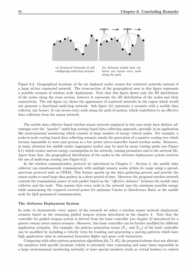
90 Chapter 6. Concluding Remarks
(a) Scattered Networks in selfconfiguring multi-hop scenario
(b) Airborne mobile data col-lector can access every nodealong the path
Figure 6.2: Geographical locations of the air deployed nodes creates few scattered networks instead ofa large ad-hoc connected network. The cross-section of the geographical area in this figure representsa possible scenario of wireless node deployment. Note that this figure shows only the 2D distributionof the nodes along the cross section, however it represents the 3D distribution of the nodes and theirconnectivity. The sub figure (a) shows the appearance of scattered networks in the region which wouldnot generate a functional multi-hop network. Sub figure (b) represents a scenario with a mobile datacollector (air borne). It can access every node along the path of motion, which contributes to an effectivedata collection from the sensor network.
The mobile data collector based wireless sensor network employed in this case study have distinct ad-vantages over the “popular” multi-hop routing based data collecting approach, specially in an applicationlike environmental monitoring which consists of large number of energy critical nodes. For example, anode-to-node routing based data collecting scenario entails the generation of a massive routing tree whichbecome impossible to store and process in a low power micro-controller based wireless nodes. Moreover,in many situation few middle nodes (aggregator nodes) may be used by many routing paths (see Figure6.1) which creates uneven energy consumption in the network, causing premature end to the network life.Apart from that, the geographical distribution of the nodes in the airborne deployment system restrictsthe use of multi-hop routing (see Figure 6.2).
In the wireless communication protocol we introduced in Chapter 5 - Section 2, the mobile datacollector can simultaneously communicate with multiple sensory nodes within its range using a spread-spectrum protocol such as CDMA. This feature speeds up the data gathering process and provide thesensor nodes to send large data packets in a short period of time. Moreover the proposed wireless networkcontrols the transmission power of each packet based on the “effective distance” between the mobile datacollector and the node. This ensures that every node in the network uses the minimum possible energywhile maintaining the required received power for optimum Carrier to Interference Ratio at the mobilenode for QoS guaranteed communication.
The Airborne Deployment System
In order to demonstrate every aspect of the research we select a wireless sensor network deploymentscenario based on the swarming guided weapon system introduced in the chapter 4. Note that thecontroller for guided weapon system is derived from the basic controller (see chapter 3) introduced for ageneric swarm robot control scenario. Moreover, this basic controller can be further modified for differentapplication scenarios. For example, the pattern generation terms (Fi,r and Fi,a) of the basic controllercan be modified by including a velocity term for tracking and generating a moving patterns which havehigh application value in automated formation flights and space craft formations.
Comparing with other pattern generation algorithms [64, 71, 65], the proposed scheme does not allocatethe members with specific locations (which is extremely time consuming and some times impossible ina large environmental monitoring network) or have special members (such as virtual leaders) to control

Chapter 6. Concluding Remarks 91
sections of the swarm. This eliminates any scalability and robustness issues which are inherent to suchcentralized systems. On the other hand, in our algorithm, the members are driven by a decentralizedcontroller (every member uses the same controller and same weighing parameters) which navigate theentire airborne sensor system as a group eliminating the necessities for special members or to derivemember specific weighing parameters.
An airborne wireless sensor node is basically a flying platform similar to a guided weapon (glided);containing the navigation controller, self localization capabilities (such as GPS and inertial), sensor devicesand wireless communication equipments. Unlike the guided weapon navigation mechanisms, which needsto navigate a massive weapon with pin point accuracy, the navigation system in a airborne wireless sensornetwork deployment needs fairly simple control mechanisms in order to guide the light weight target.However, we do not discuss the hardware development of such airborne sensor in this dissertation andpropose it as further work that could be done in parallel with this research.
In relation with the wireless sensor network deployment, the airborne sensors need to be informed withthe desired geographical area (as a sequence of points representing the contour of the region - see figure4.13) and the weighing parameters for pattern generation (according to the selection criteria proposed inthe chapter 4). Moreover, we provided a lower bound for the release height (hrel) of the swarm, whichguarantee that every sensor node drops inside the desired area when released higher than hrel. The controlscheme however does not include any compensation for natural effects such as wind and up-drifts whichmay cause the airborne system to navigate in an unpredictable manner, and they are identified as furtherimprovements in this scheme.
Internal Communications
Another important component in navigating the airborne sensor system is the internal communicationscheme which is used to share location information of the entire swarm. Instantaneous knowledge ofthe positions of the other members is utmost important for an airborne unit in avoiding collision amongmembers as well as distributing the sensor network evenly within the desired geographical area. Theall-to-all communication algorithm proposed in the chapter 5 (section 1) can be identified as the bestcandidate for such information sharing scheme. Since the proposed communication scheme enables aswarm member to send its location (and status) information to the entire swarm while receiving thesame information from the others at the same time, it satisfies the condition “instantaneous knowledgeof the location of the entire swarm”, which is a major assumption in the pattern generation theory.Moreover, the scheme provides with single-hop broadcasting methodology, which eliminate the routingtree generation in an mobile ad-hoc network as well as the delays occurred in a routing based data sharingalgorithms. Furthermore, the communication scheme is optimized for battery life as well as the QoS ofthe communication links.
Final Remark
The above describes a potential application scenario which uses the aspects of the entire research /thesis. However, there are many other instances which can employ the findings of this research eitherpartially or completely. Although this dissertation provides a solid foundation to a pattern generation(populate members inside a shape contour) solution, there exists many potential future work which willinevitably add extra application value. Among them, real-world implementation of the swarm robotcontrol algorithm can be identified as a major portion. This could be done for either ground or airbornesystem, which include specific hardware platform development and controller modification for kinematicsof the target platform.

Appendix I: Mathematical Function for
Contour Generation
For the simulation of the algorithm, the contour γ s are generated by a mathematical function in the
following form,
� (γ(θ)) = d
((a− b)cos(θ) + c cos
((a− b)θ
b
))(6.0.1)
� (γ(θ)) = d
((a− b)sin(θ) − c sin
((a− b)θ
b
)). (6.0.2)
The parameter a ∈ determines the number of edges in the contour. Parameter b = 1 for a simple closed
contour and c determines the smoothness of the edges (c > 1 makes the edges to wind, c = 1 makes sharp
edges and c < 1 results in round edges with c = 0 making a circle). Parameter d > 0 determines the
overall size of the shape.
Table 6.1: Properties of the function
Parameter a Shape No of symmetrical axes
3 Triangular 3
4 Rectangular 4
. . .
8 Octagonal 8
. . .
92

Bibliography
[1] E. Sahin, “Swarm robotics: From sources of inspiration to domains of application,” in Swarm
Robotics, ser. Lecture Notes in Computer Science, 2005, pp. 10–20.
[2] L. Bayindir and E. Sahin, “A review of studies in swarm robotics,” Turk J Elec Engin, vol. 15,
no. 2, pp. 115–147, 2007.
[3] V. Gazi and B. Fidan, “Coordination and control of multi-agent dynamic systems: Models and
approaches,” in Swarm Robotics, ser. Lecture Notes in Computer Science, 2007, pp. 71–102.
[4] S. W. Ekanayake and P. N. Pathirana, “Artificial formation forces for stable aggregation of multi-
agent system,” in Information and Automation, 2006. ICIA 2006. International Conference on,
2006, pp. 129–134.
[5] ——, “Smart cluster bombs - control of multi-agent systems for military applications,” in Network-
ing, Sensing and Control, 2007 IEEE International Conference on, 2007, pp. 471–476.
[6] ——, “Geometric formations in swarm aggregation: An artificial formation force based approach,”
in Information and Automation for Sustainability, 2007. ICIAfS 2007. International Conference on.
[7] ——, “Two stage architecture for navigating multiple guided weapons into a widespread target,” in
IEEE Aerospace conference 2008, BigSky, Montana, USA.
[8] S. W. Ekanayake, P. N. Pathirana, and M. Palanaswami, “Maintaining optimal co-channel interfer-
ence for power efficient wireless communication,” in ISSNIP conference 2007, Melbourne, Australia.
[9] S. W. Ekanayake, P. N. Pathirana, B. F. Rolfe, and M. Palanaswami, “Energy efficient, fully-
connected mesh networks for high speed applications,” in IEEE Vehicular Technology Conference,
VTC2008, Singapore.
93

94 Bibliography
[10] U. http://www.shef.ac.uk/marcoms/eview/articles58/robot.htm, “A 13th century programmable
robot,” The University of Sheffield, 2007.
[11] M. E. Rosheim, Leonardos Lost Robots, 1st ed. Springer Berlin Heidelberg, 2006.
[12] U. http://www.robotics.utexas.edu/rrg/learn more/history, “Robotics Research Group- Learn
More History,” The University of Texas at Austin, 2007.
[13] R. Whiting, The Art of Leonardo Da Vinci - A portrait of the Renaissance man. London: Quantum
Publishing Ltd, 2005.
[14] M. Rosheim, “In the footsteps of leonardo [articulated anthropomorphic robot],” Robotics & Au-
tomation Magazine, IEEE, vol. 4, no. 2, pp. 12–14, Jun 1997.
[15] E. Bonabeau, M. Dorigo, and G. Theraulaz, Swarm intelligence: from natural to artificial systems.
US: Oxford University Press, 1999.
[16] J. Kennedy, Swarm Intelligence, ser. Handbook of Nature-Inspired and Innovative Computing, 2006.
[17] E. Bonabeau and C. Meyer, “Swarm intelligence: A whole new way to think about business,”
Harward Business Review, pp. 106–114, May 2001.
[18] M. Dorigo and G. D. Caro, “The ant colony optimization meta-heuristic,” New ideas in optimization,
pp. 11–32, 1999.
[19] M. Dorigo and T. Sttzle, Ant Colony Optimization. MIT Press, 2004.
[20] A. Ratnaweera, S. Halgamuge, and H. Watson, “Self-organizing hierarchical particle swarm opti-
mizer with time-varying acceleration coefficients,” Evolutionary Computation, IEEE Transactions
on, vol. 8, no. 3, pp. 240–255, June 2004.
[21] M. Clerc, Particle Swarm Optimization. ISTE Publishing Company, 2006.
[22] F. Mondada, L. Gambardella, D. Floreano, S. Nolfi, J. Deneuborg, and M. Dorigo, “The coopera-
tion of swarm-bots: physical interactions in collective robotics,” Robotics & Automation Magazine,
IEEE, vol. 12, pp. 21–28, 2005.
[23] G. Beni, “From swarm intelligence to swarm robotics,” in Swarm Robotics, 2005, pp. 1–9.
[24] M. Krieger, J. Billeter, and L. Keller, “Ant-like task allocation and recruitment in cooperative
robots,” Nature, vol. 406, pp. 992–995, August 2000.

Bibliography 95
[25] D. M. Gordon, “The organization of work in social insect colonies,” Complexity, vol. 8(1), pp. 43–46,
2003.
[26] I. Hamilton and L. Dill, “Group foraging by a kleptoparalastic fish: A strong inference test of social
foraging models,” Ecology, vol. 84(12), pp. 3349–3359, 2003.
[27] E. Robinson, D. Jackson, M. Holcomber, and F. Ratnieks, “’no entry’ signal in ant foraging,”
Nature, vol. 438, p. 442, November 2005.
[28] C. Brown and K. Warburton, “Social mechanisms enhance escape responses in schoals of rainbow-
fish,” Environmental Biology of Fishes, vol. 56, pp. 455–459, 1999.
[29] Y. Inada, “Steering mechanisms in fish schools,” Complexity International, vol. 8, pp. 43–46, 2001.
[30] S. V. Grnbaum, D. and J. K. Parrish, “Extracting interactive control algorithms from group dy-
namics of schooling fish,” in Cooperative Control, ser. Lecture Notes in Control and Information
Sciences. Berlin / Heidelberg: Springer, 2004, vol. 309, pp. 103–117.
[31] C. Parker and H. Zhang, “Collective robotic site preparation,” Adaptive Behavior, vol. 14, no. 1,
pp. 5–19, 2006.
[32] C. W. Reynolds, “Flocks, Herds, and Schools: A Distributed Behavioral Model,” Computer Graph-
ics, vol. 21, no. 4, pp. 25–34, 1987.
[33] R. Burton, Bird Behavior. Alfred A. Knopf, Inc, 1985.
[34] B. Partridge, “Structure and function of fish schools,” Scientific American, pp. 114–123, June 1982.
[35] C. Breder, “Equations descriptive of fish schools and other animal aggregations,” Ecology, vol. 35,
no. 3, pp. 361–370, 1954.
[36] A. Okubo, “Dynamical Aspects of animal grouping: swarms, schools, flocks, and herds,” Advances
in Biophysics, vol. 22, pp. 1–94, 1986.
[37] K. Warburton and J. Lazarus, “Tendency-distance models of social cohesion in animal groups,”
Journal of Theoretical Biology, vol. 150, pp. 473–488, 1991.
[38] D. Grunbaum and A. Okubo, “Modelling social animal aggregations,” in Frontiers in Theoretical
Biology, ser. Lecture notes in Biomathematics. Springer-Verlag, New York, 1994, pp. 296–325.

96 Bibliography
[39] V. Gazi and K. Passino, “A class of attraction/repulsion functions for stable swarm aggregations,”
Decision and Control, 2002, Proceedings of the 41st IEEE Conference on, vol. 3, pp. 2842–2847,
2002.
[40] ——, “Stability analysis of swarms,” Automatic Control, IEEE Transactions on, vol. 48, pp. 692–
697, 2003.
[41] V. Gazi, “Swarm aggregations using artificial potentials and sliding-mode control,” Robotics, IEEE
Transactions on [see also Robotics and Automation, IEEE Transactions on], vol. 21, Issue 6, pp.
1208–1214, 2005.
[42] V. Gazi and K. Passino, “Stability analysis of social foraging swarms,” Systems, Man and Cyber-
netics, Part B, IEEE Transactions on, vol. 34, pp. 539–557, 2004.
[43] L. Yang, K. Passino, and M. Polycarpou, “Stability analysis of m-dimensional asynchronous swarms
with a fixed communication topology,” Automatic Control, IEEE Transactions on, vol. 48, pp. 76–
95, 2003.
[44] Y. Liu and K. Passino, “Stable social foraging swarms in a noisy environment,” Automatic Control,
IEEE Transactions on, vol. 49, Issue 1, pp. 30–44, 2004.
[45] L. Yang, K. Passino, and M. Polycarpou, “Stability analysis of one-dimensional asynchronous
swarms,” Automatic Control, IEEE Transactions on, vol. 48, pp. 1848–1854, 2003.
[46] O. Soysal and E. Sahin, “Probabilistic aggregation strategies in swarm robotic systems,” Swarm
Intelligence Symposium, Proceedings 2005 IEEE, pp. 325–332, June 2005.
[47] V. Trianni, T. Labella, R. Grob, E. Sahin, M. Dorigo, and J. Deneubourg, “Modeling Pattern
Formation in a Swarm of Self-Assembling Robots,” Technical Report TR/IRIDIA/2002-12, IRIDIA,
Universit Libre de Bruxelles, Bruxelles, Belgium, May 2002.
[48] K. Naruse, H. Yokoi, M. Kinoshita, and Y. Kakazu, “Group formation of agents with two-
dimensional inner state and one-to-one subjective evaluation,” Proceedings IEEE International
Symposium on Computational Intelligence in Robotics and Automation ,, vol. 3, pp. 1492– 1497,
2003.
[49] E. Bahceci and E. Sahin, “Evolving aggregation behaviors for swarm robotic systems: A systematic
case study,” Swarm Intelligence Symposium, Proceedings 2005 IEEE.

Bibliography 97
[50] V. Trianni, R. Grob, T. Labella, E. Sahin, and M. Dorigo, “Evolving Aggregation Behaviors in a
Swarm of Robots,” in Advances in Artificial Life - Proceedings of the 7th Europian Conference on
Artificial Life (ECAL), ser. Lecture notes in Artificial Intelligence. Springer Verlag, Heidelberg,
Germany, 2003, pp. 865–874.
[51] T. Vicsek, A. Czirok, E. Ben-Jacob, I. Cohen, and O. Shochet, “Novel type of phase transition in
a system of self-driven particles,” Phys. Rev. Lett., vol. 75, no. 6, pp. 1226–1229, Aug 1995.
[52] A. Jadbabaie, J. Lin, and A. Morse, “Coordination of groups of mobile autonomous agents using
nearest neighbor rules,” Automatic Control, IEEE Transactions on, vol. 48, no. 6, pp. 988–1001,
June 2003.
[53] R. Olfati-Saber, “Flocking for multi-agent dynamic systems: Algorithms and theory,” IEEE Trans-
actions on Automatic Control, vol. 51, pp. 401–420, March 2006.
[54] A. Tanner, Herbert G.and Jadbabaie and G. J. Pappas, “Flocking in Teams of Nonholonomic
Agents,” in in S. Morse, N. Leonard and V. Kumar (eds.), Cooperative Control, ser. Lecture Notes
in Control and Information Sciences. Springer-Verlag, 2005, pp. 229–239.
[55] H. Tanner, A. Jadbabaie, and G. Pappas, “Stable flocking of mobile agents part i: dynamic topol-
ogy,” Decision and Control, 2003. Proceedings. 42nd IEEE Conference on, vol. 2, pp. 2016–2021,
9-12 Dec. 2003.
[56] ——, “Stable flocking of mobile agents, part i: fixed topology,” Decision and Control, 2003. Pro-
ceedings. 42nd IEEE Conference on, vol. 2, pp. 2010–2015, 9-12 Dec. 2003.
[57] H. Ando, Y. Oasa, I. Suzuki, and M. Yamashita, “Distributed memoryless point convergence algo-
rithm for mobile robots with limited visibility,” Robotics and Automation, IEEE Transactions on,
vol. 15, no. 5, pp. 818–828, Oct 1999.
[58] J. Lin, A. Morse, and B. Anderson, “The multi-agent rendezvous problem,” Decision and Control,
2003. Proceedings. 42nd IEEE Conference on, vol. 2, pp. 1508–1513, 9-12 Dec. 2003.
[59] ——, “The multi-agent rendezvous problem - the asynchronous case,” Decision and Control, 2004.
CDC. 43rd IEEE Conference on, vol. 2, pp. 1926–1931, 14-17 Dec. 2004.
[60] G. Conte and P. Pennesi, “On convergence conditions for rendezvous,” Decision and Control, 2007
46th IEEE Conference on, pp. 2375–2378, 12-14 Dec. 2007.

98 Bibliography
[61] A. Tiwari, J. Fung, I. Carson, J.M., R. Bhattacharya, and R. Murray, “A framework for lyapunov
certificates for multi-vehicle rendezvous problems,” American Control Conference, 2004. Proceedings
of the 2004, vol. 6, pp. 5582–5587, 30 June-2 July 2004.
[62] Y. Q. Chen and Z. Wang, “Formation control: a review and a new consideration,” Intelligent Robots
and Systems, 2005. (IROS 2005). 2005 IEEE/RSJ International Conference on, pp. 3181– 3186,
2005.
[63] G. Antonelli and S. Chiaverini, “Kinematic control of platoons of autonomous vehicles,” Robotics,
IEEE Transactions on, December 2006.
[64] J. Desai, J. Ostrowski, and V. Kumar, “Controlling formations of multiple mobile robots,” Proc.
IEEE Int. Conf. Robotics Automation, Leuven, Belgium, pp. 2864–2869, 1998.
[65] H. Tanner, G. Pappas, and V. Kumar, “Leader-to-formation stability,” Robotics and Automation,
IEEE Transactions on, vol. 29, pp. 443–455, 2004.
[66] V. Gazi, “Formation control of a multi-agent system using decentralized nonlinear servomechanism,”
Decision and Control, 2003. Proceedings. 42nd IEEE Conference on, vol. 3, pp. 2531–2536, 2003.
[67] N. Leonard and E. Fiorelli, “Virtual leaders, artificial potentials and coordinated control of groups,”
Decision and Control, 2001. Proceedings of the 40th IEEE Conference on, vol. 3, pp. 2968–2973,
2001.
[68] M. Egerstedt and X. Hu, “Formation constrained multi-agent control,” Robotics and Automation,
IEEE Transactions on, vol. 17, pp. 947–951, 2001.
[69] X. Xi and E. Abed, “Formation control with virtual leaders and reduced communications,” Decision
and Control, 2005. Proceedings of the 44th IEEE Conference on, pp. 1854–1860, 2005.
[70] H. Hsu and A. Liu, “Applying a taxonomy of formation control in developing a robotic system,”
Tools with Artificial Intelligence, 2005. ICTAI 05. 17th IEEE International Conference on, pp.
3–10, 2005.
[71] J. Spletzer and R. Fierro, “Optimal positioning strategies for shape changes in robot teams,”
Robotics and Automation, 2005. ICRA 2005. Proceedings of the 2005 IEEE International Con-
ference on, pp. 742–747, 2005.

Bibliography 99
[72] T. Balch and R. Arkin, “Behavior-based formation control for multirobot teams,” Robotics and
Automation, IEEE Transactions on, vol. 14, pp. 926–939, 1998.
[73] K. Sugihara and I. Suzuki, “Distributed algorithms for formation of geometric patterns with many
mobile robots,” Journal of Robotic Systems, vol. 13, no. 3, pp. 127–139, 1996.
[74] I. Suzuki and M. Yamashita, “Distributed autonomous mobile robots: Formation of geometric
patterns,” SIAM J Comput, vol. 29, no 4, pp. 1347–1363, 1999.
[75] W. Spears, D. Spears, J. Hamann, and R. Heil, “Distributed, physics-based control of swarms of
vehicles,” Autonomous Robots, vol. 17, no. 2, pp. 137–162, 2004.
[76] S. Nouyan and M. Dorigo, “Chain formation in a swarm of robots,” IRIDIA, Universite Libre de
Bruxelles, Tech. Rep. TR/IRIDIA/2004-18, March 2004.
[77] R. Grob, M. Bonani, F. Mondada, and M. Dorigo, “Autonomous self-assembly in a swarmbot,” Pro-
ceedings of the third international symposium on autonomous minirobots for research edutainment,
pp. 314–322, 2006.
[78] D. Payton, M. Dally, R. Estkowski, M. Howard, and C. Lee, “Pheromone robotics,” Autonomous
Robots, vol. 11, no. 3, pp. 314–322, 2001.
[79] D. Payton, R. Estkowski, and M. Howard, “Pheromone robotics and the logic of virtual
pheromones,” SAB 2004, pp. 45–57, 2004.
[80] W. Shen, C. Chuong, and P.Will, “Simulating self-organization for multi-robot systems,” Interna-
tional Conference on Intelligent and Robotic Systems, 2002.
[81] W. Shen, P. Will, A. Galstyan, and C. Chuong, “Hormone-inspired self-organization and distributed
control of robotic swarms,” Autonomous Robots, vol. 17, pp. 93–105, 2004.
[82] J. Reif and H. Wang, “Social potential fields: A distributed behavioral control for autonomous
robots,” Robot. Auton. Syst., vol. 8, no. 5, pp. 171–194, 1999.
[83] D. Kim, H. Wang, G. Ye, and S. Shin, “Decentralized control of autonomous swarm systems using
artificial potential functions: Analytical design guidelines,” 43rd IEEE Conference on Decision and
Control, Atlantis, Paradise Island, Bahamas, pp. 159–164, 2004.

100 Bibliography
[84] T. Tsuji, Y. Tanaka, P. Morasso, V. Sanguineti, and M. Kaneko, “Bio-mimetic trajectory generation
of robots via artificial potential field with time base generator,” IEEE Transactions on Systems,
Man, and Cybernetic-Part C: Applications and Reviews, vol. 32, no. 4, pp. 426–439, 2002.
[85] L. Chaimowicz, N. Michael, and V. Kumar, “Controlling swarms of robots using interpolated implicit
functions,” Proc. IEEE Int. Conf. Robotics Automation, Barcelona, Spain, pp. 2487–2492, 2005.
[86] V. Gazi and K. Passino, “A class of attraction/repulsion functions for stable swarm aggregations,”
Decision and Control, 2002, Proceedings of the 41st IEEE Conference on, vol. 3, pp. 2842–2847,
10-13 Dec. 2002.
[87] R. Bachmayer and N. Leonard, “Vehicle networks for gradient decent in a sampled environment,”
Decision and Control, 2002. Proceedings of the 40th IEEE Conference on, pp. 112–117, 2002.
[88] W. Spears and D. Gordon, “Using artificial physics to control agents,” Information Intelligence and
Systems, 1999. Proceedings. 1999 International Conference on, pp. 281–288, 1999.
[89] W. M. Spears, D. F. Spears, R. Heil, W. Kerr, and S. Hettiarachchi, “An overview of physicomimet-
ics,” Lecture Notes in Computer Science, Swarm Robotics, pp. 84–97, 2005/// 2005.
[90] W. Spears, D. Spears, and R. Heil, “A formal analysis of potential energy in a multi-agent system,”
Lecture Notes in Computer Science, Formal Approaches to Agent-Based Systems, pp. 131–145, 2005.
[91] D. Spears, D. Zarzhitsky, and D. Thayer, “Multi-robot chemical plume tracing,” Multi-Robot Sys-
tems. From Swarms to Intelligent Automata, vol. III, pp. 211–221, 2005.
[92] D. Zarzhitsky, D. Spears, D. Thayer, and W. Spears, “Agent-based chemical plume tracing using
fluid dynamics,” Lecture Notes in Computer Science, Formal Approaches to Agent-Based Systems,
pp. 146–160, 2005.
[93] D. Zarzhitsky, D. Spears, W. Spears, and D. Thayer, “A fluid dyanmics approach to multi-robot
chemical plume tracing,” Autonomous Agents and Multiagent Systems, 2004. AAMAS 2004. Pro-
ceedings of the Third International Joint Conference on, pp. 1476–1477, 2004.
[94] T. Balch, F. Dellaert, A. Feldman, A. Guillory, J. Isbell, C.L., Z. Khan, S. Pratt, A. Stein, and
H. Wilde, “How multirobot systems research will accelerate our understanding of social animal
behavior,” Proceedings of the IEEE, vol. 94, no. 7, pp. 1445–1463, 2006.

Bibliography 101
[95] C. Harper and A. Winfield, “A methodology for provably stable intelligent control,” Robotics and
Autonomous Systems, vol. 54, no. 1, pp. 52–73, 2006.
[96] S. Gueron and S. Levin, “The dynamics of group formation,” Mathematical Biosciences, vol. 128,
pp. 243–264, 1995.
[97] O. Soysal and E. Sahin, “A macroscopic model for probabilistic aggregation in swarm robotic
systems,” In Sahin et al., E., ed.: Proc of SAB06 Workshop on Swarm Robotics. Lecture Notes in
Computer Science (LNCS), Springer Verlag, 2006.
[98] W. Agassounon, A. Martinoli, and K. Easton, “Macroscopic modeling of aggregation experiments
using embodied agents in teams of constant and time-varying sizes,” Autonomous Robots, vol. 17,
no. 2-3.
[99] R. Goebel, C. Prieur, and A. Teel, “Smooth patchy control lyapunov functions,” Decision and
Control, 2006 45th IEEE Conference on, pp. 3271–3276, 2006.
[100] P. Ogren, M. Egerstedt, and X. Hu, “A control lyapunov function approach to multi-agent coor-
dination,” Decision and Control, 2001. Proceedings of the 40th IEEE Conference on, vol. 2, pp.
1150–1155, 2001.
[101] ——, “A control lyapunov function approach to multiagent coordination,” Robotics and Automation,
IEEE Transactions on, vol. 18, no. 5, pp. 847–851, 2002.
[102] J. Desai, J. Ostrowski, and V. Kumar, “Modeling and control of formations of nonholonomic mobile
robots,” Robotics and Automation, IEEE Transactions on, vol. 17, no. 6, pp. 905–908, Dec 2001.
[103] W. Dong and Y. Guo, “Formation control of nonholonomic mobile robots using graph theoretical
methods,” Applied Optimization, Cooperative Control and Optimization, pp. 369–386, 2007.
[104] R. Fierro, P. Song, A. Das, and V. Kumar, “Cooperative control of robot formations,” Lecture Notes
in Economics and Mathematical System, Cooperative Systems, pp. 73–93, 2002.
[105] J. Desai, “Modeling multiple teams of mobile robots: a graph theoretic approach,” Intelligent Robots
and Systems, 2001. Proceedings. 2001 IEEE/RSJ International Conference on, vol. 1, pp. 381–386,
2001.
[106] J. La Salle and S. Lefschetz, Stability by Liapunov’s Direct Method With Applications, ser. Mathe-
matics in Science and Engineering. Academic Press Inc (London) Ltd., 1967, vol. 4.

102 Bibliography
[107] R. Horn and C. Johnson, Matrix Analysis. Cambridge: Cambridge University Press, 1985.
[108] R. S. Varga, Matrix Iterative Analysis, ser. Prentis Hall Series in Automaic Computation. N.J.:
Prentis Hall, Inc., 1962.
[109] M.-Y. A. Hsieh and V. Kumar, “Pattern generation with multiple robots,” Proc. IEEE Int. Conf.
Robotics Automation, Orlando, Florida, pp. 2442–2447, 2006.
[110] D. Holeman, “Impact of 1-meter GPS navigation on war fighting,” Position Location and Navigation
Symposium, 1996., IEEE 1996, pp. 530–537, Apr 1996.
[111] G. Graham and A. Killen, “GPS navigation requirements for future mobile ground-based missile
systems,” in Position Location and Navigation Symposium, 1992. Record. ’500 Years After Columbus
- Navigation Challenges of Tomorrow’. IEEE PLANS ’92., IEEE, 1992, pp. 419–421.
[112] E. Gai, “The century of inertial navigation technology,” in Aerospace Conference Proceedings, 2000
IEEE, vol. 1, 2000, pp. 59–60 vol.1.
[113] R. Bajaj, S. L. Ranaweera, and D. P. Agrawal, “GPS: Location-tracking technology,” Computer,
pp. 92–94, April 2002.
[114] “Aviation electronics/avionics,” Aerospace and Electronic Systems Magazine, IEEE, vol. 15, no. 10,
pp. 47–61, 2000.
[115] D. Pedlar and D. Coe, “Target geolocation using SAR,” Radar, Sonar and Navigation, IEE Pro-
ceedings -, vol. 152, no. 1, pp. 35–42, 2005.
[116] J. Sherman, R. Davis, W. Owens, and J. Valdes, “The autonomous underwater glider ”spray”,”
Oceanic Engineering, IEEE Journal of, vol. 26, no. 4, pp. 437–446, 2001.
[117] J. Goodman, “Application of GPS navigation to space flight,” in Aerospace, 2005 IEEE Conference,
2005, pp. 1837–1852.
[118] X. Lin, T. Kirubarajan, Y. Bar-Shalom, and X. Li, “Enhanced accuracy GPS navigation using the
interacting multiple model estimator,” in Aerospace Conference, 2001, IEEE Proceedings., vol. 4,
2001, pp. 4/1911–4/1923 vol.4.
[119] D. Pittman and C. Roberts, “Determining GPS anti-jamming performance on tactical missiles,” in
Position Location and Navigation Symposium, 1994., IEEE, 1994, pp. 641–648.

Bibliography 103
[120] W. Caldwell, “Analysis of mission computer utilization of the GPS navigation solution during a
simulated fighter/attack scenario,” in Position Location and Navigation Symposium, 1988. Record.
’Navigation into the 21st Century’. IEEE PLANS ’88., IEEE, 1988, pp. 165–170.
[121] T. Loffler and J. Nielson, “International harm precision navigation upgrade. a GPS/INS missile
upgrade that improves effectiveness and minimizes friendly-fire accidents,” in Position Location and
Navigation Symposium, 2002 IEEE, 2002, pp. 106–112.
[122] G. Hyslop, D. Gerth, and J. Kraemer, “GPS/INS integration on the standoff land attack missile
(slam),” Aerospace and Electronic Systems Magazine, IEEE, vol. 5, no. 7, pp. 29–34, 1990.
[123] ——, “GPS/INS integration on the standoff land attack missile (slam),” in Position Location and
Navigation Symposium, 1990. Record. ’The 1990’s - A Decade of Excellence in the Navigation
Sciences’. IEEE PLANS ’90., IEEE, 1990, pp. 407–412.
[124] P. Renfroe, J. McMinemon, and P. Couch, “Test and evaluation of the rockwell collins GNP-10
for the precision kill and targeting (PKAT) missile system,” in Position Location and Navigation
Symposium, IEEE 2000, 2000, pp. 488–493.
[125] A. Gamble and P. Jenkins, “Low cost guidance for the multiple launch rocket system (MLRS)
artillery rocket,” in Position Location and Navigation Symposium, IEEE 2000, 2000, pp. 193–199.
[126] B. Nguyen, Y.-L. Chuang, D. Tung, C. Hsieh, Z. Jin, L. Shi, D. Marthaler, A. Bertozzi, and
R. Murray, “Virtual attractive-repulsive potentials for cooperative control of second order dynamic
vehicles on the caltech mvwt,” American Control Conference, 2005. Proceedings of the 2005, vol. 2,
pp. 1084–1089, 2005.
[127] S. S. Ge, C.-H. Fua, and W.-M. Liew, “Swarm formations using the general formation potential
function,” Robotics, Automation and Mechatronics, 2004 IEEE Conference on, vol. 2, pp. 655–600,
2004.
[128] F. Ganji and S. Joshi, “Adaptive formation control for rovers travelling over unknown terrain,”
Journal of Guidance, Control and Dynamics, vol. 29, no. 3, pp. 714–724, May-June 2006.
[129] W. Ren and R. Beard, “Decentralized scheme for spacecraft formation flying via the virtual structure
approach,” Journal of Guidance, Control and Dynamics, vol. 27, no. 1, pp. 73–82, January-February
2004.

104 Bibliography
[130] M. Patcher, J. D’Azzo, and A. Proud, “Tight formation flight control,” Journal of Guidance, Control
and Dynamics, vol. 24, no. 2, pp. 246–254, March-April 2001.
[131] E. Yang, Y. Masuko, and T. Mita, “Dual controller approach to three-dimensional autonomous
formation control,” Journal of Guidance, Control and Dynamics, vol. 27, no. 3, pp. 336–346, May-
June 2004.
[132] R. Sattigeri and A. Calise, “An adaptive vision-based approach to decentralized formation control,”
Journal of Aerospace Computing, Information and Communication, vol. 1, pp. 502–525, December
2004.
[133] D. Stilwell, B. Bishop, and C. Sylvester, “Redundant manipulator techniques for partially decentral-
ized path planning and control of a platoon of autonomous vehicles,” Systems, Man and Cybernetics,
Part B, IEEE Transactions on, vol. 35, no. 4, pp. 842–848, 2005.
[134] B. Bishop, “On the use of redundant manipulator techniques for control of platoons of cooperating
robotic vehicles,” Systems, Man and Cybernetics, Part A, IEEE Transactions on, vol. 33, no. 5, pp.
608–615, 2003.
[135] H. Yamaguchi and J. Burdick, “Asymptotic stabilization of multiple nonholonomic mobile robots
forming group formations,” in Robotics and Automation, 1998. Proceedings. 1998 IEEE Interna-
tional Conference on, vol. 4, 1998, pp. 3573–3580.
[136] F. Giulietti, L. Pollini, and M. Innocenti, “Autonomous formation flight,” IEEE Control Systems
Magazine, pp. 34–44, December 2000.
[137] S. Kalantar and U. Zimmer, “Contour shaped formation control for autonomous underwater vehicles
using canonical shape descriptors and deformable models,” OCEANS ’04. MTS/ IEEE TECHNO-
OCEAN ’04, pp. 296–307, 2004.
[138] S. Ekanayake and P. Pathirana, “Smart cluster bombs - control of multi-agent systems for military
applications,” Proc. IEEE Int. Conf. Network, Sensing and Control, London, UK, pp. 471–476,
April 2007.
[139] B. Lubachevsky and R. Graham, “Curved hexagonal packings of equal disks in a circle,” Discrete
& Computational Geometry, vol. 18, pp. 197–194, 1997.

Bibliography 105
[140] P. Szab, T. Csendes, L. Casado, and I. Garca, “Packing equal circles in a square i. - problem set-
ting and bounds for optimal solutions,” Optimization Theory: Recent Developments from Mtrahza,
vol. 18, pp. 191–206, 2001.
[141] Y. Hwang and N. Ahuja, “A potential field approach to path planning,” Robotics and Automation,
IEEE Transactions on, vol. 8, no. 1, pp. 23–32, 1992.
[142] O. Khatib, “Real-time obstacle avoidance for manipulators and mobile robots,” in Robotics and
Automation. Proceedings. 1985 IEEE International Conference on, vol. 2, 1985, pp. 500–505.
[143] ——, “Real-time obstacle avoidance for manipulators and mobile robots,” vol. 5, no. 1, pp. 90–98,
1986.
[144] M. G. Park, J. H. Jeon, and M. C. Lee, “Obstacle avoidance for mobile robots using artificial
potential field approach with simulated annealing,” in Industrial Electronics, 2001. Proceedings.
ISIE 2001. IEEE International Symposium on, vol. 3, 2001, pp. 1530–1535 vol.3.
[145] J. Schiller, Mobile Communications, 2nd ed. Addison-Wesley, 2003.
[146] R. Bruno, M. Conti, and E. Gregori, “Mesh networks: commodity multihop ad hoc networks,”
Communications Magazine, IEEE, vol. 43, no. 3, pp. 123–131, 2005.
[147] M. Lee, J. Zheng, Y.-B. Ko, and D. Shrestha, “Emerging standards for wireless mesh technology,”
Wireless Communications, IEEE [see also IEEE Personal Communications], vol. 13, no. 2, pp.
56–63, 2006.
[148] J. Jun and M. Sichitiu, “The nominal capacity of wireless mesh networks,” Wireless Communica-
tions, IEEE [see also IEEE Personal Communications], vol. 10, no. 5, pp. 8–14, 2003.
[149] R. Hincapie, J. Sierra, and R. Bustamante, “Remote locations coverage analysis with wireless mesh
networks based on ieee 802.16 standard,” Communications Magazine, IEEE, vol. 45, no. 1, pp.
120–127, 2007.
[150] K. Almeroth, “The evolution of multicast: from the mbone to interdomain multicast to internet2
deployment,” Network, IEEE, vol. 14, no. 1, pp. 10–20, 2000.
[151] Y. Chan, J. Modestino, Q. Qu, and X. Fan, “An end-to-end embedded approach for multi-
cast/broadcast of scalable video over multiuser cdma wireless networks,” Multimedia, IEEE Trans-
actions on, vol. 9, no. 3, pp. 655–667, 2007.

106 Bibliography
[152] M.-S. Chen, J.-C. Chen, and P. Yu, “On general results for all-to-all broadcast,” Parallel and
Distributed Systems, IEEE Transactions on, vol. 7, no. 4, pp. 363–370, 1996.
[153] Y. Yang and J. Wang, “Pipelined all-to-all broadcast in all-port meshes and tori,” Transactions on
Computers, vol. 50, no. 10, pp. 1020–1032, 2001.
[154] W. Jia, L. Cheng, and G. Xu, “Efficient multicast routing algorithms on mesh networks,” Algorithms
and Architectures for Parallel Processing, 2002. Proceedings. Fifth International Conference on, pp.
110–117, 2002.
[155] S.-C. Kim and K. Shin, “A performance analysis of manet multicast routing algorithms with multiple
sources,” Software Engineering Research, Management & Applications, 2007. SERA 2007. 5th ACIS
International Conference on, pp. 73–82, 20-22 Aug. 2007.
[156] I. F. Akyildiz, E. Ekici, and G. Yue, “A distributed multicast routing scheme for multi-layered
satellite ip networks,” Wireless Networks, vol. 9, no. 5, pp. 535–544, 2003.
[157] S. Guo and O. Yang, “A constraint formulation for minimum-energy multicast routing in wireless
multihop ad-hoc networks,” Wireless Networks, vol. 12, no. 1, pp. 23–32, 2006.
[158] M. Transier, H. Fubler, J. Widmer, M. Mauve, and W. Effelsberg, “A hierarchical approach to
position-based multicast for mobile ad-hoc networks,” Wireless Networks, vol. 13, no. 4, pp. 447–
460, 2007.
[159] L.-L. Yang, “Mimo-assisted space-code-division multiple-access: linear detectors and performance
over multipath fading channels,” Selected Areas in Communications, IEEE Journal on, vol. 24,
no. 1, pp. 121–131, 2006.
[160] Y. Yang and J. Wang, “On blocking probability of multicast networks,” Communications, IEEE
Transactions on, vol. 46, no. 7, pp. 957–968, 1998.
[161] ——, “Near-optimal all-to-all broadcast in multidimensional all-port meshes and tori,” Parallel and
Distributed Systems, IEEE Transactions on, vol. 13, no. 2, pp. 128–141, 2002.
[162] F. Ellersick, “A conversation with claude shannon,” Communications Magazine, IEEE, vol. 22,
no. 5, pp. 123–126, 1984.
[163] G. Cooper and R. Nettleton, “A spread-spectrum technique for high-capacity mobile communica-
tions,” Vehicular Technology, IEEE Transactions on, vol. 27, no. 4, pp. 264–275, 1978.

Bibliography 107
[164] R. Prasad and T. Ojanpera, “A survey on cdma: evolution towards wideband cdma,” in Spread
Spectrum Techniques and Applications, 1998. Proceedings., 1998 IEEE 5th International Symposium
on, vol. 1, 1998, pp. 323–331 vol.1.
[165] R. Scholtz, “The evolution of spread-spectrum multiple-access communications,” in Spread Spectrum
Techniques and Applications, 1994. IEEE ISSSTA ’94., IEEE Third International Symposium on,
1994, pp. 4–13 vol.1.
[166] D. Knisely, S. Kumar, S. Laha, and S. Nanda, “Evolution of wireless data services: Is-95 to
cdma2000,” Communications Magazine, IEEE, vol. 36, no. 10, pp. 140–149, 1998.
[167] K. Gilhousen, I. Jacobs, R. Padovani, A. Viterbi, J. Weaver, L.A., and I. Wheatley, C.E., “On the
capacity of a cellular cdma system,” Vehicular Technology, IEEE Transactions on, vol. 40, no. 2,
pp. 303–312, 1991.
[168] J. Zander, “Performance of optimum transmitter power control in cellular radio systems,” Vehicular
Technology, IEEE Transactions on, vol. 41, no. 1, pp. 57–62, 1992.
[169] S. Grandhi, R. Vijayan, D. Goodman, and J. Zander, “Centralized power control in cellular radio
systems,” Vehicular Technology, IEEE Transactions on, vol. 42, no. 4, pp. 466–468, 1993.
[170] S. Grandhi, R. Vijayan, and D. Goodman, “Distributed power control in cellular radio systems,”
Communications, IEEE Transactions on, vol. 42, no. 234, pp. 226–228, 1994.
[171] S. Grandhi, R. Yates, and D. Goodman, “Resource allocation for cellular radio systems,” Vehicular
Technology, IEEE Transactions on, vol. 46, no. 3, pp. 581–587, 1997.
[172] G. Foschini and Z. Miljanic, “A simple distributed autonomous power control algorithm and its
convergence,” vol. 42, pp. 249–257, 2004.
[173] Z. Uykan and H. Koivo, “Sigmoid-basis nonlinear power-control algorithm for mobile radio systems,”
Vehicular Technology, IEEE Transactions on, vol. 53, no. 1, pp. 265–270, 2004.
[174] ——, “Proportional power control algorithm for time varying link gains in cellular radio systems,”
Vehicular Technology, IEEE Transactions on, vol. 55, no. 1, pp. 341–349, 2006.
[175] M. Cai, W. Wang, and H. S. Zhang, “Power control algorithm for time-varying cdma cellular sys-
tems,” Proceedings of 2004 International Conference on Intelligent Mechatronics and Automation,
pp. 605–610, 2004.
108 Bibliography
[176] D. Vengerov, N. Bambos, and H. Berenji, “A fuzzy reinforcement learning approach to power control
in wireless transmitters,” Systems, Man and Cybernetics, Part B, IEEE Transactions on, vol. 35,
no. 4, pp. 768–778, 2005.
[177] Y. Hou, Y. Shi, J. Pan, and S. Midkiff, “Maximizing the lifetime of wireless sensor networks through
optimal single-session flow routing,” Mobile Computing, IEEE Transactions on, vol. 5, no. 9, pp.
1255–1266, 2006.
[178] T. Klein and H. Viswanathan, “Centralized power control and routing policies for multihop wireless
networks,” Information Theory, IEEE Transactions on, vol. 52, no. 3, pp. 849–866, 2006.
[179] T. ElBatt and A. Ephremides, “Joint scheduling and power control for wireless ad hoc networks,”
Wireless Communications, IEEE Transactions on, vol. 3, no. 1, pp. 74–85, 2004.
[180] Y. Zhou, M. Lyu, and J. Liu, “On setting up energy-efficient paths with transmitter power con-
trol in wireless sensor networks,” in Mobile Adhoc and Sensor Systems Conference, 2005. IEEE
International Conference on, 2005, p. 9 pp.
[181] J. Gomez and A. Campbell, “Variable-range transmission power control in wireless ad hoc net-
works,” Mobile Computing, IEEE Transactions on, vol. 6, no. 1, pp. 87–99, 2007.
[182] P. Nar and E. Cayirci, “PCSMAC: a power controlled sensor-MAC protocol for wireless sensor
networks,” in Wireless Sensor Networks, 2005. Proceeedings of the Second European Workshop on,
2005, pp. 81–92.
[183] S. Lin, J. Zhang, G. Zhou, L. Gu, J. A. Stankovic, and T. He, “ATPC: adaptive transmission power
control for wireless sensor networks http://doi.acm.org/10.1145/1182807.1182830,” in Proceedings
of the 4th international conference on Embedded networked sensor systems. Boulder, Colorado,
USA: ACM Press, 2006, pp. 223–236.
[184] S. Lim, K. Leong, and T. Itoh, “Adaptive power controllable retrodirective array system for wireless
sensor server applications,” Microwave Theory and Techniques, IEEE Transactions on, vol. 53,
no. 12, pp. 3735–3743, 2005.
[185] V. Erceg, L. Greenstein, S. Tjandra, S. Parkoff, A. Gupta, B. Kulic, A. Julius, and R. Bianchi, “An
empirically based path loss model for wireless channels in suburban environments,” Selected Areas
in Communications, IEEE Journal on, vol. 17, no. 7, pp. 1205–1211, 1999.
Bibliography 109
[186] R. Santos, O. Alvarez, and A. Edwards, “Experimental analysis of wireless propagation models with
mobile computing applications,” in Electrical and Electronics Engineering, 2005 2nd International
Conference on, 2005, pp. 40–43.
[187] W. Tam and V. Tran, “Propagation modelling for indoor wireless communication,” Electronics &
Communication Engineering Journal, vol. 7, no. 5, pp. 221–228, 1995.
[188] R. Sato, H. Sato, and H. Shirai, “A SBR estimation for indoor wave propagation through dielectric
walls,” in Antennas and Propagation Society International Symposium, 2005 IEEE, vol. 2B, 2005,
pp. 719–722 vol. 2B.
[189] D. Puccinelli and M. Haenggi, “Multipath fading in wireless sensor networks: measurements and in-
terpretation http://doi.acm.org/10.1145/1143549.1143757,” in Proceeding of the 2006 international
conference on Communications and mobile computing. Vancouver, British Columbia, Canada:
ACM Press, 2006, pp. 1039–1044.
[190] V. Degli-Esposti, G. Lombardi, and C. Passerini, “Measurement and ray-tracing prediction of indoor
channel parameters,” Electronics Letters, vol. 34, no. 22, pp. 2167–2168, 1998.
[191] K. Remley, H. Anderson, and A. Weisshar, “Improving the accuracy of ray-tracing techniques for
indoor propagation modeling,” Vehicular Technology, IEEE Transactions on, vol. 49, no. 6, pp.
2350–2358, 2000.
[192] F. Agelet, F. Fontan, and A. Formella, “Fast ray tracing for microcellular and indoor environments,”
Magnetics, IEEE Transactions on, vol. 33, no. 2, pp. 1484–1487.
[193] Crossbow Technologies Incorporated, “http://www.xbow.com.”
[194] “C2240 Transceiver Datasheet,” Chipcon Systems, 2004.


![Cloud Networked Robotics - Teknologisk Institut Networked Robotics.pdf · expansion of such robotic middleware as ROS [3] or RT-Middleware [4]. Since such ... of robots on cloud servers,](https://img.pdfslide.us/doc/110x75/5ad65c807f8b9a5d058e6241/cloud-networked-robotics-teknologisk-networked-roboticspdfexpansion-of-such-robotic.jpg)