Biol. Cybern. 61, 89-101 (1989) Biological Cybernetics �9 Springer-Verlag 1989

Formation and Control of Optimal Trajectory in Human Multijoint Arm Movement

Minimum Torque-Change Model

Y. Uno*, M. Kawato**, and R. Suzuki***

Department of Biophysical Engineering, Faculty of Engineering Science, Osaka University, Toyonaka, Osaka, 560 Japan

Abstract. In this paper, we study trajectory planning and control in voluntary, human arm movements. When a hand is moved to a target, the central nervous system must select one specific trajectory among an infinite number of possible trajectories that lead to the target position. First, we discuss what criterion is adopted for trajectory determination. Several resear- chers measured the hand trajectories of skilled move- ments and found common invariant features. For example, when moving the hand between a pair of targets, subjects tended to generate roughly straight hand paths with bell-shaped speed profiles. On the basis of these observations and dynamic optimization theory, we propose a mathematical model which accounts for formation of hand trajectories. This model is formulated by defining an objective function, a measure of performance for any possible movement: square of the rate of change of torque integrated over the entire movement. That is, the objective function C T is defined as follows:

Cr= 2 i= t \ dt ] dt ,

where z i is the torque generated by the i-th actuator (muslce) out of n actuators, and t: is the movement time. Since this objective function critically depends on the complex nonlinear dynamics of the musculo- skeletal system, it is very difficult to determine the unique trajectory which yields the best performance.

* Present address: Department of Mathematical Engineering and Information Physics, Faculty of Engineering, University of Tokyo, Hongo, Bunkyo-ku, Tokyo, 113 Japan ** Present address: ATR Auditory and Visual Perception

Research Laboratories, Cognitive Processes Department, Twin 21 Bldg. MID Tower, 2-1-61 Shiromi, Higashi-ku, Osaka, 540 Japan *** Present address: Department of Mathematical Engineering and Information Physics, Faculty of Engineering, University of Tokyo, Hongo, Bunkyo-ku, Tokyo, 113 Japan

We overcome this difficult by developing an iterative scheme, with which the optimal trajectory and the associated motor command are simultaneously com- puted. To evaluate our model, human hand trajec- tories were experimentally measured under various behavioral situations. These results supported the idea that the human hand trajectory is planned and con- trolled in accordance with the minimum torque- change criterion.

I Introduction

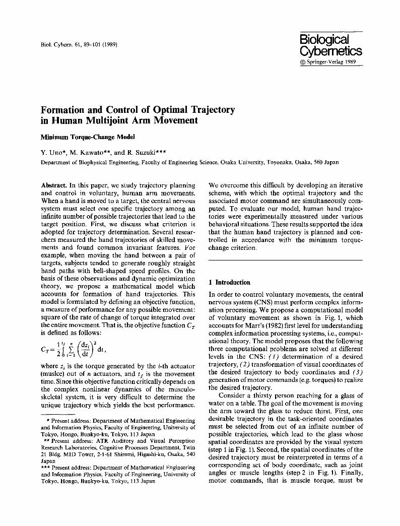
In order to control voluntary movements, the central nervous system (CNS) must perform complex inform- ation processing. We propose a computational model of voluntary movement as shown in Fig. 1, which accounts for Marr's (1982) first level for understanding complex information processing systems, i.e., comput- ational theory. The model proposes that the following three computational problems are solved at different levels in the CNS: (1) determination of a desired trajectory, (2) transformation of visual coordinates of the desired trajectory to body coordinates and (3) generation of motor commands (e.g. torques) to realize the desired trajectory.

Consider a thirsty person reaching for a glass of water on a table. The goal of the movement is moving the arm toward the glass to reduce thirst. First, one desirable trajectory in the task-oriented coordinates must be selected from out of an infinite number of possible trajectories, which lead to the glass whose spatial coordinates are provided by the visual system (step 1 in Fig. 1). Second, the spatial coordinates of the desired trajectory must be reinterpreted in terms of a corresponding set of body coordinate, such as joint angles or muscle lengths (step 2 in Fig. 1). Finally, motor commands, that is muscle torque, must be

90

s tep 1

s t e p 5

-trajectory determination

.coordinates transformation

-generation of motor command step 4

�9 coordinates [ t~ansformatlon i

.generation of motor command

step 2 step 3

Fig. 1. A computational model for voluntary movement

generated to coordinate the activity of many muscles so that the desired trajectory is realized (step 3 in Fig. 1). It must be noted that we do not adhere to the hypothesis of the step-by-step information processing (i.e. step 1 ~ 2 ~ 3 ) shown by the bottom line of this figure. Rather, our model indicates that there are other information processings (step 4 and step 5 in Fig. 1) which realize the desired trajectory. In step 4, the motor command can be obtained directly from the desired trajectory represented in the task-oriented coordinates: that is, the two problems (coordinate transformation and generation of motor command) are simultaneously solved. Further, in step 5, the motor command is calculated directly from the goal of movement: that is, the three problems (trajectory formation, coordinate transformation and generation of motor command) are simultaneously solved.

We will mainly discuss the first problem (trajectory determination) out of the three computational pro- blems and develop an algorithm that corresponds to step 5 in Fig. 1. The other two problems (coordinates transformation and generation of motor command) have been discussed in earlier papers (Kawato et al. 1987, 1988a, b).

In this paper, the term "trajectory" refers to path and speed of movement: the path is a sequence of positions that the hand follows in space, and the speed is a time sequence of movement velocity along the path.

Early studies of the motor control have concen- trated on single-joint arm movements (e.g. Polite and Bizzi 1979; Bizzi et al. 1984). Whereas, recently, several studies have been reported regarding the kinematic and dynamic aspects of multijoint arm movements. For multijoint arm movements, there exist new control problems that do not exist in the single-joint case (Hollerbach and Flash 1982). Even a two-joint move- ment is vastly more complicated than a single-joint movement because of the presence of interactional forces (e.g. Colioris forces, reaction foces and centrip-

etal forces). When the hand of the multijoint arm is moved from one position to another, there are an infinite number of possible paths which lead to the final position. What strategy does the CNS use to determine a desired trajectory? In what coordinates frame is the trajectory planned?

Morasso (1981) provided experimental data which suggests that the desired treajectory is first planned at the task-oriented (visual) coordinates. He measured human two-joint arm movements restricted to an horizontal plane, and found the following common invariant kinematic features. When a subject was instructed merely to move his hand from one visual target to another, his hand usually moved along a roughly straight path with a bell-shaped speed profile. Morasso also reported that, in contrast to the simple hand profile, the angular positions and velocity pro- files of the two joints (shoulder and elbow) were widely different according to the parts of the work-space in which movements were performed. These results pro- vide strong support for the hypothesis that arm movements are planned in terms of the hand kinema- tics at the task-oriented coordinates rather than joint rotations at the body coordinates.

Abend et al. (1982) investigated not only straight paths but also curved paths. When a subject was asked merely to move his hand from one target to another, his hand path was roughly straight and the associated speed had a single-peaked profile, that was entirely consistent with Morasso's experiment. In contrast to the point-to-point movements, when the subject was instructed to move his hand while avoiding an obstacle or along a self-generated curved path, the hand path appeared to be composed of a series of gently curved segments and the speed profile had often several peaks. In this case, the curved path usually contained distinct curvature peaks which were temporally associated with valleys in the hand speed profile.

In order to account for these kinematic features, Flash and Hogan (1985) proposed a mathematical

91

model, "minimum jerk model". The minimum jerk model is formulated by defining the following objective function, a measure of performance for any possible movement: square of the jerk (rate of change of acceleration) of the hand position integrated over the entire movement. Flash and Hogan showed that the unique trajectory which yields the best performance was in good agreement with experimental data in some region of the work-space. Their analysis was based solely on the kinematics of movement and independent of the dynamics of the musculoskeletal system.

On the other hand, considering the dynamics of the arm, a few researchers proposed several performance indices for trajectory formation, though their studies were restricted to single-joint movements. Nelson (1983) computed the trajectories which minimized various measures of physical cost (for example, move- ment time, maximum force, impulse, energy etc.), and compared the resulting trajectories with each other. Hasan (1986) gave a criterion function which was the time integral of the product of muscle stiffness and square of the time differential of the equilibrium trajectory. But it is not clear whether their analyses can be applied to multijoint arm movements.

Presuming that the objective function must be related to the dynamics, we (Uno et al. 1987) proposed the following measure of a performance index: sum of square of the rate of change of torque integrated over the entire movement. Here, let us call this model "minimum torque-change model". Regarding the move- ments which were examined by Morasso (1981) and Abend et al. (1982), the hand trajectories predicted by the minimum torque-change model are in fairly good agreement with those of the minimum jerk model. However, under several behavioral situations, the predictions of these two models are quite different. These two models are investigated in detail and compared with each other on the basis of our experi- mental data about human planar arm movements.

2 Minimum Torque-Change Model

Skilled movements are in general extremely smooth and graceful. Hogan (1984) proposed a single organiz- ing principle to predict the qualitative and quantitative features of single-joint forearm movements, assuming that maximizing smoothness may be equivalent to minimizing the mean-square jerk. Here, jerk is math- ematically defined as the rate of change of acceleration.

Flash and Hogan (1985) generalized this organiz- ing principle to multijoint motion, using dynamic optimization theory. Dynamic optimization requires the definition of a objective function (criterion func- tion), which is generally expressed as a time integral of

a performance index. Taking account of the kinematic features of the motion and the suggestion that move- ments are planned in terms of hand trajectories rather than joint rotations, Flash and Hogan adopted the Cartesian jerk of the hand as the performance index. In moving from an initial to a final position in a given time ts, the criterion function to be minimized is expressed as follows:

Cd= 1 t f ~(d3x~2 (d3y~2~ 2 o [ k d ~ - / + k, d f ~ / J dt. (2.1)

Here, (x, y) is the Cartesian coordinates of the hand position.

The criterion function determines the form of the movement trajectory. The methods of variational calculus and optimal control theory (Bryson and Ho 1975) were applied to find mathematical expressions for x(t) and y(t), which minimize the criterion function Cs. If the boundary conditions at the onset and termination of the movement are given, the criterion function Cs determines the form of the hand trajectory completely. Assuming the movement to start and end with zero velocity and acceleration, the following expression for hand trajectory are obtained:

x(t) = Xo + (Xo - xy) (15z 4 - 6z s - 10z 3) (2.2)

y(t) = Yo + (Yo -- Yl) (15z 4 - 6z 5 - - 1 0 z 3 ) ,

where z = t/ty, (xo, Yo) is the initial hand position at t=0, and (xy, yy) is the final hand position at t - - t y (Flash and Hogan 1985).

One can easily see that the path derived from (2.2) is a straight line between the initial and the final positions and the associated speed profile is bell-shaped. This model predicted and reproduced the qualitative fea- tures and the quantitative details of the human hand trajectories between two targets which are located approximately in front of the body (Flash and Hogan 1985; Fig. 3). Furthermore, the minimum jerk model successfully reproduced a curved movement through a certain via-point as well as a stright movement be- tween two points (Flash and Hogan 1985: Figs. 5-7).

Since x(t) and y(t) depend only on the initial and final positions of the hand and movement time, the optimal trajectory is determined only by the kinema- tics of the hand in the task-oriented coordinates and is independent of the physical system which generates the motion. In this way, the minimum jerk model is consistent with the hypothesis that the desired trajec- tory is first planned at the task-oriented (visual) coordinates. However, it seems very strange that the optimal trajectory of our voluntary movement is determined perfectly independent of the dynamical quantities such as arm length, payload, motor com- mand, torque or external force etc.

92

On the basis of the idea that the criterion function must be related to some physical variables concerning the dynamics of the controlled object, we examined a few kinds of performance indices (e.g. energy, torque, movement time etc.). As a result of these investigations, we propose the minimum torque-change model, which is formulated by the following performance index:

CT= ,~1 dt. (2.3)

Here, z i is the motor command (torque) fed to the i-th actuator (muscle) out of n actuators. The criterion function C w is the sum of square of the rate of change of torque integrated over the entire movement. One can easily see that the two objective functions C s and CT are closely related, because acceleration is locally proportional to torque at zero speed.

3 Predictions of Minimum Torque-Change Model

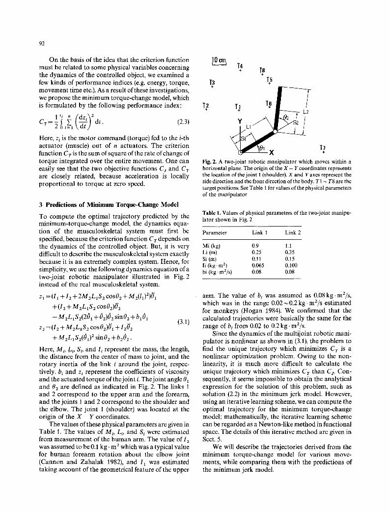
To compute the optimal trajectory predicted by the minimum-torque-change model, the dynamics equa- tion of the musculoskeletal system must first be specified, because the criterion function CT depends on the dynamics of the controlled object. But, it is very difficult to describe the musculoskeletal system exactly because it is an extremely complex system. Hence, for simplicity, we use the following dynamics equation of a two-joint robotic manipulator illustrated in Fig. 2 instead of the real musculoskeletal system.

Z 1 = (11 + 12 + 2M2L1S 2 cos 0 2 q- M2(11)2)0.1

+(12 + M2L1S2 C O S 0 2 ) 0 . 2

- MEL1S2(201 + 02)02 sin0z + b101 (3.1)

Z 2 ~--" (12 + M2LIS 2 cos 02)0.1 -t- 120" 2

+ M2L1S2(O1) 2 sin02 + b202.

Here, M i, .Li, S i, and I i represent the mass, the length, the distance from the center of mass to joint, and the rotary inertia of the link i around the joint, respec- tively, bi and z i represent the coefficients of viscosity and the actuated torque of the joint i. The joint angle 01 and 02 are defined as indicated in Fig. 2. The links 1 and 2 correspond to the upper arm and the forearm, and the joints 1 and 2 correspond to the shoulder and the elbow. The joint 1 (shoulder) was located at the origin of the X - Y coordinates.

The values of these physical parameters are given in Table 1. The values of Mi, Li, and S~ were estimated from measurement of the human arm. The value of 12 was assumed to be 0.1 kg- m 2 which was a typical value for human forearm rotation about the elbow joint (Cannon and Zahalak 1982), and 11 was estimated taking account of the geometrical feature of the upper

10 cm I I

T3 §

T?

T4 § T8

§

T+I T+6 Z L2

T1 §

Fig. 2. A two-joint robotic manipulator which moves within a horizontal plane. The origin of the X - Y coordinates represents the location of the joint 1 (shoulder). X and Y axes represent the side direction and the front direction of the body. T1 ~ T8 are the target positions. See Table 1 for values of the physical parameters of the manipulator

Table 1. Values of physical parameters of the two-joint manipu- lator shown in Fig. 2

Parameter Link 1 Link 2

Mi (kg) 0.9 1.1 Li (m) 0.25 0.35 Si (m) 0.11 0.15 Ii (kg. m 2) 0.065 0.100 bi (kg. mZ/s) 0.08 0.08

arm. The value of b i was assumed as 0.08 kg. mZ/s, which was in the range 0.02,-~ 0.2 kg. ma/s estimated for monkeys (Hogan 1984). We confirmed that the calculated trajectories were basically the same for the range of b i from 0.02 to 0.2 kg. m2/s.

Since the dynamics of the multijoint robotic mani- pulator is nonlinear as shown in (3.1), the problem to find the unique trajectory which minimizes CT is a nonlinear optimization problem. Owing to the non- linearity, it is much more difficult to calculate the unique trajectory which minimizes CT than Ca. Con- sequently, it seems impossible to obtain the analytical expression for the solution of this problem, such as solution (2.2) in the minimum jerk model. However, using an iterative learning scheme, we can compute the optimal trajectory for the minimum torque-change model; mathematically, the iterative learning scheme can be regarded as a Newton-like method in functional space. The details of this iterative method are given in Sect. 5.

We will describe the trajectories derived from the minimum torque-change model for various move- ments, while comparing them with the predictions of the minimum jerk model.

93

a b

T~] e~" ....... /+T5 ~1 // ""

......... :3,.,~......'.]'Z ":.--_~, T6 (time) T2 C T1

d

0 Y ~" /--~.. X "1 \'

'SOOmsec path

A

C

/ ',, '500msec

e f

�9 ,. / / \,,

'5oo~ %oo~J speed

a b

......... -'Z'=.~:.,',jF: "7, ~ 'S0(]msec ~ i i ~T6 (time)

d Y

o x

path

c ] //2' ~ i':

.7 ~OOm~

e f

speed

B

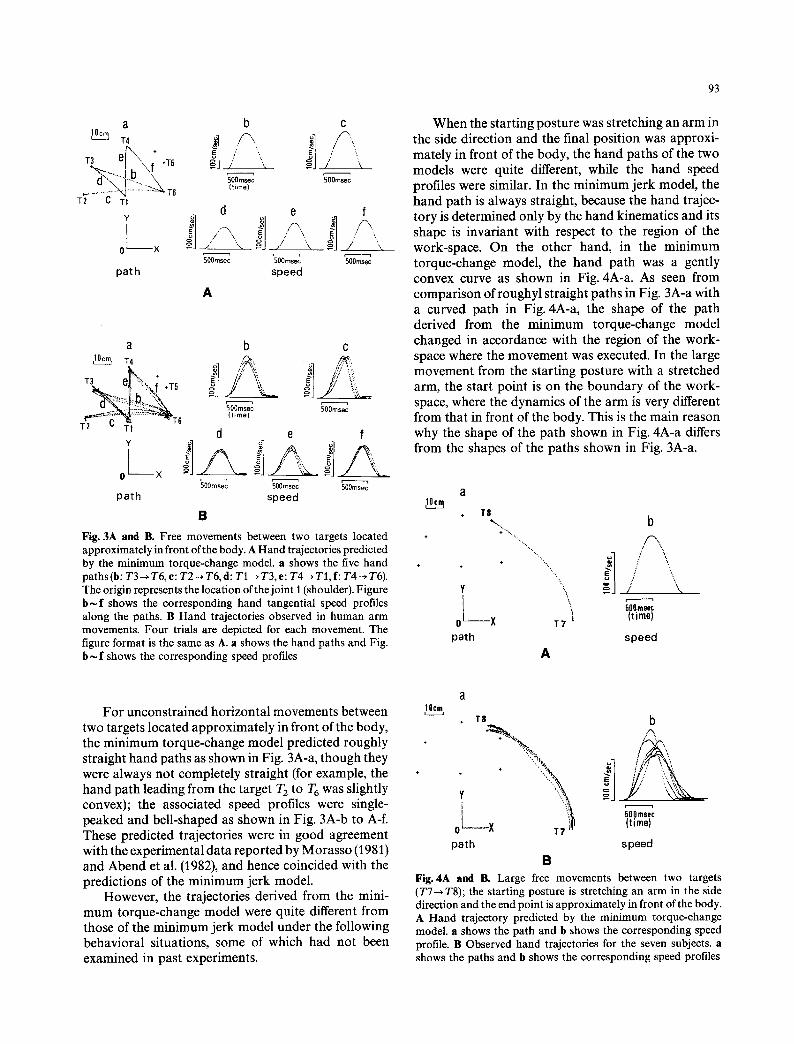
Fig. 3A and B. Free movements between two targets located approximately in front of the body. A Hand trajectories predicted by the minimum torque-change model, a shows the five hand paths(h: T3--* T6, e: T2--* T6, d: T1 ~ T 3 , e : T4~T1 , f: T4-* T6). The origin represents the location of the joint 1 (shoulder). Figure h ~ f shows the corresponding hand tangential speed profiles along the paths. B Hand trajectories observed in human arm movements. Four trials are depicted for each movement. The figure format is the same as A. a shows the hand paths and Fig. h ~ f shows the corresponding speed profiles

When the starting posture was stretching an arm in the side direction and the final position was approxi- mately in front of the body, the hand paths of the two models were quite different, while the hand speed profiles were similar. In the minimum jerk model, the hand path is always straight, because the hand trajec- tory is determined only by the hand kinematics and its shape is invariant with respect to the region of the work-space. On the other hand, in the minimum torque-change model, the hand path was a gently convex curve as shown in Fig. 4A-a. As seen from comparison of roughyl straight paths in Fig. 3A-a with a curved path in Fig. 4A-a, the shape of the path derived from the minimum torque-change model changed in accordance with the region of the work- space where the movement was executed. In the large movement from the starting posture with a stretched arm, the start point is on the boundary of the work- space, where the dynamics of the arm is very different from that in front of the body. This is the main reason why the shape of the path shown in Fig. 4A-a differs from the shapes of the paths shown in Fig. 3A-a.

a

§

§

T8 %. b

�9 ......,.. ~" ,,. '.~

' 50Omsec X 7 7 I ( t ime) o

path speed A

For unconstrained horizontal movements between two targets located approximately in front of the body, the minimum torque-change model predicted roughly straight hand paths as shown in Fig. 3A-a, though they were always not completely straight (for example, the hand path leading from the target T 2 to T 6 was slightly convex); the associated speed profiles were single- peaked and bell-shaped as shown in Fig. 3A-b to A-f. These predicted trajectories were in good agreement with the experimental data reported by Morasso (1981 ) and Abend et al. (1982), and hence coincided with the predictions of the minimum jerk model.

However, the trajectories derived from the mini- mum torque-change model were quite different from those of the minimum jerk model under the following behavioral situations, some of which had not been examined in past experiments.

10cm

+

+

§ T8

�9 '"~":%j,

.

path

B

b

500 rnsec (time)

speed

Fig. 4A and B. Large free movements between two targets (T7--*T8); the starting posture is stretching an arm in the side direction and the end point is approximately in front of the body. A Hand trajectory predicted by the minimum torque-change model, a shows the path and h shows the corresponding speed profile. B Observed hand trajectories for the seven subjects, a shows the paths and h shows the corresponding speed profiles

94

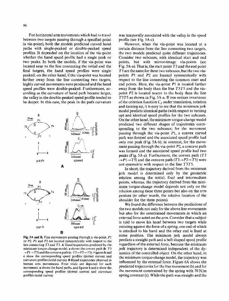
For horizontal arm movements which had to travel between two targets passing through a specified point (a via-point), both the models predicted curved hand paths with single-peaked or double-peaked speed profiles. It depended on the location of the via-point whether the hand speed profile had a single peak or two peaks. In both the models, if the via-point was located near to the line connecting the initial and the final targets, the hand speed profiles were single peaked; on the other hand, if the via-point was located further away from the line connecting two targets, highly curved movements were produced and the hand speed profiles were double-peaked. Furthermore, ac- cording as the curvature of hand path became larger, the valley in the double-peaked speed profile tended to be deeper. In this case, the peak in the path curvature

a

, § §

Y

ol x

pa th

b

... ;, \ s k

' ' ' ' ( t i m e ) "~ ' - 500reset ~ ,~

C/~

'500msec s p e e d

A

b a /"~ , 0 c . p , _

":~" b ~ . . . . . . % 8 ....... [~

500 msec g pat h speed

B Fig. 5A and B. Free movements passing through a via-point, P1 or P2. P1 and P2 are located symmetrically with respect to the line connecting T3 and T5. A Hand trajectories predicted by the minimum torque-change model, a shows the convex path (b: T3

P I ~ T5) and the concave path (e: T3 ~ P 2 ~ T5). Figures b and e show the corresponding speed profiles (dotted curves) and curvature profiles (solid curves). B Hand trajectories observed in human arm movements. Four trials are depicted for each movement, a shows the hand paths, and figures b and e show the corresponding speed profiles (dotted curves) and curvature profiles (solid curves)

was temporally associated with the valley in the speed profile (see Fig. 5A-c).

However, when the via-point was located at a certain distance from the line connecting two targets, the two models predicted quite different trajectories. Consider two subcases, with identical start and end points, but with mirror-image via-points (see Fig. 5A-a). That is, the start point T3 and the end point T5 are the same for these two subcases, but the two via- points P1 and P2 are located symmetrically with respect to the line connecting the common start and end points. Here, the via-point P1 is located further away from the body than the line T3 T5 and the via- point P2 is located nearer to the body than the line T3T5 as shown in Fig. 5A-a. If one notices invariance of the criterion function Cs under translation, rotation and turning up, it is easy to see that the minimum jerk model predicts identical paths (with respect to turning up) and identical speed profiles for the two subcases. On the other hand, the minimum torque-change model predicted two different shapes of trajectories corre- sponding to the two subcases; for the movement passing through the via-point P1, a convex curved path was formed and the associated speed profile had only one peak (Fig. 5A-b); in contrast, for the move- ment passing through the via-point P2, a concave path was formed and the associated speed profile had two peaks (Fig. 5A-c). Furthermore, the convex path (T3 ~P1 ~ T5) and the concave path (T3 ~ P 2 ~ T5) were not symmetric with respect to the line T3T5.

In short, the trajectory derived from the minimum jerk model is determined only by the geometric relation among the initial, final and intermediate points, whereas, the trajectory derived from the mini- mum torque-change model depends not only on the relation among these three points but also on the arm posture (in other words, the relative location of the shoulder for the three points).

We found the difference between the predictions of the two models not only for the above free movements but also for the constrained movements in which an external force acted on the arm. Consider that a subject is told to move his hand between two targets while resisting against the force of a spring, one end of which is attached to his hand and the other end is fixed at some position. The minimum jerk model always predicts a straight path and a bell-shaped speed profile regardless of the external force, because the minimum jerk trajectory is determined independent of the dy- namics of the controlled object. On the other hand, in the minimum torque-change model, the trajectory was influenced by the external force. Figure 6A shows the predicted trajectories for the free movement (b) and for the movement constrained by the spring with 70 N/m spring constant (c). While the path was straight and the

95

a IOcm i T4 %-"--.C

U",t t b

"4 71 P" j "., Y \,,

0 r ~ 500 mser x (time)

path speed

A

C

.!

::_-:J i ' '50 O reset'

a

10cm' T4.,~.;... C ~

.... } ' tL_ 0 X '5(time/00 msec' '500 reset'

path speed

B Fig. 6A and B. Free movements between two targets (b: T4--. T6) and constrained movements in which a spring force acts on the hand (e: T4-*T6). A Hand trajectories predicted by the mini- mum torque-change model, a shows the hand path of the free movement b and the hand path of the movement influenced by the spring e. Figure b and e shows the corresponding speed profiles, B Hand trajectories observed in human arm movements. Four trials are depicted for each movement, a shows the hand paths and, b and e show the corresponding speed profiles

speed profile was bell-shaped for the free movement (Fig. 6A-b), the path was curved and the speed profile was not necessarily bell-shaped for the constrained movement (Fig. 6A-c). The magnitude of spring force which acted on the hand changed with the location of the hand; for the movement shown in Fig. 6A-c, the maximum of the spring force was 10.4N and the minimum of that was 3.3 N. This magnitude of spring force was much smaller than the limit value of the real musculoskeletal system which was observed experi- mentally by Cannon and Zahalak (1982). Consequent- ly, the external force did not give overload to the musculoskeletal system.

Furthermore, for the movements executed between two targets in a vertical plane under the effect of gravity, the minimum jerk model predicts straight hand paths with bell-shaped speed profiles, which is the same result as the model predicted for the point-to- point movements in a horizontal plane. This is because

target , f

. / / /.,

a.:.

start .... Sii-D'-i-a tget x I 0 ~1

start lOcm i I

a

:..f" %t.

:.': ./.~. "~..

' 500msec' (time)

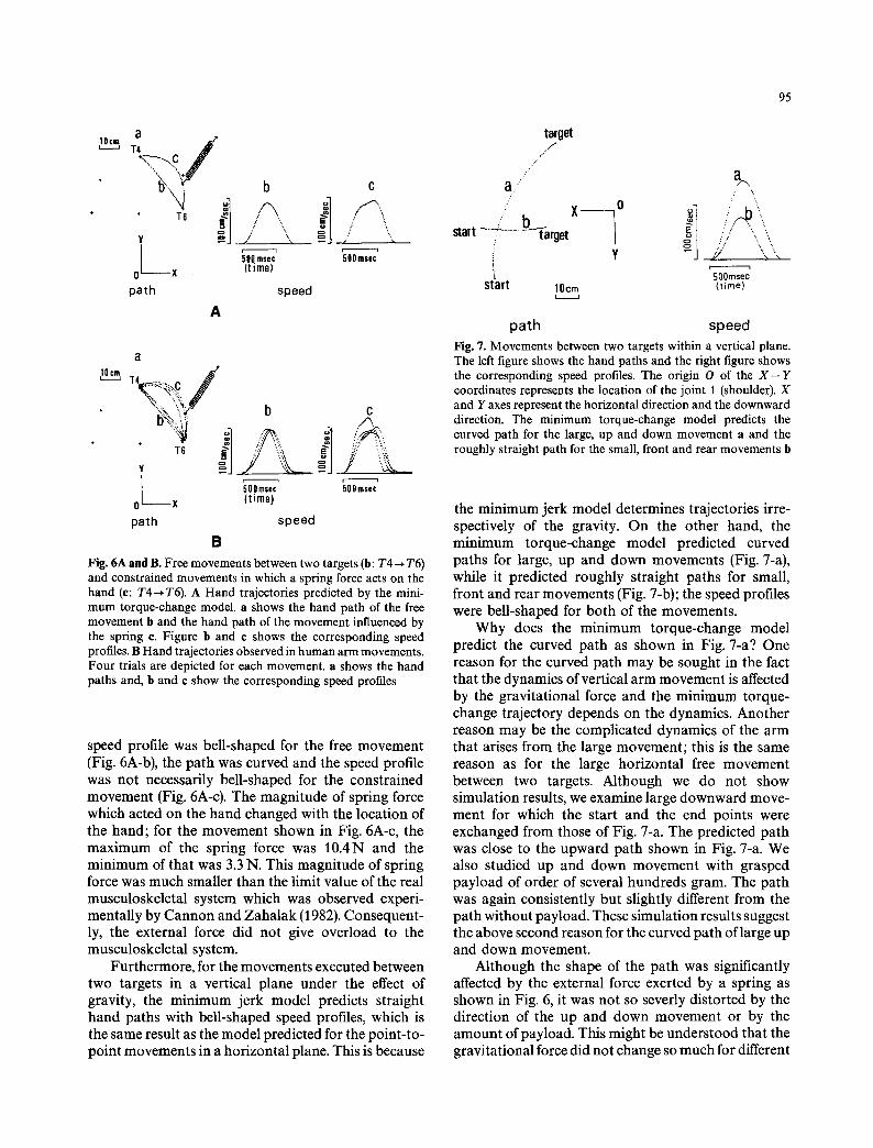
path speed Fig. 7. Movements between two targets within a vertical plane. The left figure shows the hand paths and the right figure shows the corresponding speed profiles. The origin O of the X - - Y coordinates represents the location of the joint 1 (shoulder). X and Y axes represent the horizontal direction and the downward direction. The minimum torque-change model predicts the curved path for the large, up and down movement a and the roughly straight path for the small, front and rear movements b

the minimum jerk model determines trajectories irre- spectively of the gravity. On the other hand, the minimum torque-change model predicted curved paths for large, up and down movements (Fig. 7-a), while it predicted roughly straight paths for small, front and rear movements (Fig. 7-b); the speed profiles were bell-shaped for both of the movements.

Why does the minimum torque-change model predict the curved path as shown in Fig. 7-a? One reason for the curved path may be sought in the fact that the dynamics of vertical arm movement is affected by the gravitational force and the minimum torque- change trajectory depends on the dynamics. Another reason may be the complicated dynamics of the arm that arises from the large movement; this is the same reason as for the large horizontal free movement between two targets. Although we do not show simulation results, we examine large downward move- ment for which the start and the end points were exchanged from those of Fig. 7-a. The predicted path was close to the upward path shown in Fig. 7-a. We also studied up and down movement with grasped payload of order of several hundreds gram. The path was again consistently but slightly different from the path without payload. These simulation results suggest the above second reason for the curved path of large up and down movement.

Although the shape of the path was significantly affected by the external force exerted by a spring as shown in Fig. 6, it was not so severly distorted by the direction of the up and down movement or by the amount of payload. This might be understood that the gravitational force did not change so much for different

96

postures although the spring force drastically changed with the posture. The spring force had more dramatic effect on the dynamics of manipulator and the environ- ment, so its strongly affected the shape of the path.

From the above results, we can summarize the differences between the two models as follows. The trajectories derived from the minimum jerk model are invariant with respect to the region of the work-space and independent of the external forces. On the other hand, the trajectories of the minimum torque-change model depend on the region of the work-space and are affected by the external forces.

4 Experimental Results of Human Arm Movements

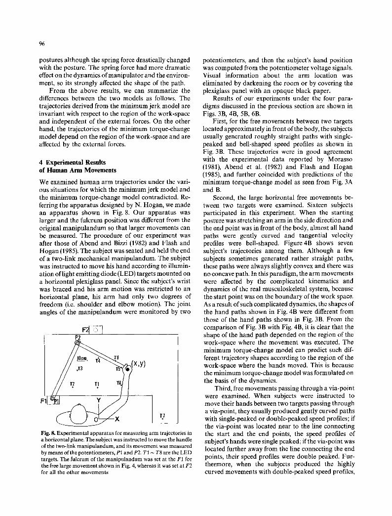
We examined human arm trajectories under the vari- ous situations for which the minimum jerk model and the minimum torque-change model contradicted. Re- ferring the apparatus designed by N. Hogan, we made an apparatus shown in Fig. 8. Our apparatus was larger and the fulcrum position was different from the original manipulandum so that larger movements can be measured. The procedure of our experiment was after those of Abend and Bizzi (1982) and Flash and Hogan (1985). The subject was seated and held the end of a two-link mechanical manipulandum. The subject was instructed to move his hand according to illumin- ation of light emitting diode (LED) targets mounted on a horizontal plexiglass panel. Since the subject's wrist was braced and his arm motion was restricted to an horizontal plane, his arm had only two degrees of freedom (i.e. shoulder and elbow motion). The joint angles of the manipulandum were monitored by two

P2

T8

F x,y) U

Fig. 8. Experimental apparatus for measuring arm trajectories in a horizontal plane. The subject was instructed to move the handle of the two-link manipulandum, and its movement was measured by means of the potentiometers, P1 and P2. T1 ~ T8 are the LED targets. The fulcrum of the manipulandum was set at the F1 for the free large movement shown in Fig. 4, whereas it was set at F2 for all the other movements

potentiometers, and then the subject's hand position was computed from the potentiometer voltage signals. Visual information about the arm location was eliminated by darkening the room or by covering the plexiglass panel with an opaque black paper.

Results of our experiments under the four para- digms discussed in the previous section are shown in Figs. 3B, 4B, 5B, 6B.

First, for the free movements between two targets located approximately in front of the body, the subjects usually generated roughly straight paths with single- peaked and bell-shaped speed profiles as shown in Fig. 3B. These trajectories were in good agreement with the experimental data reported by Morasso (1981), Abend et al. (1982) and Flash and Hogan (1985), and further coincided with predictions of the minimum torque-change model as seen from Fig. 3A and B.

Second, the large horizontal free movements be- tween two targets were examined. Sixteen subjects participated in this experiment. When the starting posture was stretching an arm in the side direction and the end point was in front of the body, almost all hand paths were gently curved and tangential velocity profiles were bell-shaped. Figure4B shows seven subject's trajectories among them. Although a few subjects sometimes generated rather straight paths, these paths were always slightly convex and there was no concave path. In this paradigm, the arm movements were affected by the complicated kinematics and dynamics of the real musculoskeletal system, because the start point was on the boundary of the work space. As a result of such complicated dynamics, the shapes of the hand paths shown in Fig. 4B were different from those of the hand paths shown in Fig. 3B. From the comparison of Fig. 3B with Fig. 4B, it is clear that the shape of the hand path depended on the region of the work-space where the movement was executed. The minimum torque-change model can predict such dif- ferent trajectory shapes according to the region of the work-space where the hands moved. This is because the minimum torque-change model was formulated on the basis of the dynamics.

Third, free movements passing through a via-point were examined. When subjects were instructed to move their hands between two targets passing through a via-point, they usually produced gently curved paths with single-peaked or double-peaked speed profiles; if the via-point was located near to the line connecting the start and the end points, the speed profiles of subject's hands were single peaked; if the via-point was located further away from the line connecting the end points, their speed profiles were double peaked. Fur- thermore, when the subjects produced the highly curved movements with double-peaked speed profiles,

97

the speed valley corresponded temporally to the curvature peak. These qualitative features were in consistent with the experimental data reported by Abend et al. (1982), although the via-point was not specified in their experiments while it was specified in our experiment. The above experimental features were consistent with the predictions of the minimum jerk model and those of the minimum torque-change model. However, when the start, the end and the via points were located at the same positions as in the simulation shown in Fig. 5A, the experimental results did not support the minimum jerk model but support the minimum torque-change model as follows.

Specifying via-points PI and P2 as shown in Fig. 5B. We measured via-point movements, T 3 ~ P 1

T5 and T3 ~ P 2 ~ T5. The convex path movements ( T 3 ~ P I ~ T 5 ) were quite different from the concave path movements ( T 3 ~ P 2 ~ T 5 ) . In particular, the speed profiles of the former were single-peaked as shown in Fig. 5B-b, while those of the latter were double-peaked as shown in Fig. 5B-c. These experi- mental results were consistent with the predictions of the minimum torque-change model.

Fourth, we measured constrained arm movements in which spring forces acted on the hands. Here the spring constant was 70 N/m, which was the same value that was specified in the predictions of the model. As shown in Fig. 6B, one end of the spring was attached to the subject's hand and the other end was fixed to the same position as in the simulation shown in Fig. 6A. The subject was asked to move his hand from initial target T4 to final target T6 while resisting against the spring force. In several trials for such movements, the subject usually generated trajectories of various shapes. However, as the subject got accustomed to the movements by repeating similar movements, he came to generate almost same trajectories for every trial. Figure 6B shows the free movement (b) and the constrained movement (c) in which the hand was moved from target T4 to T6. As seen from Fig. 6A and B, the measured hand trajectories were similar to the trajectory predicted by the minimum torque-change model.

Our experimental apparatus can not be utilized to measure arm movements within a vertical plane. Recently, Atkeson and Hollerbach (1985) measured human arm movements in three dimensional space using the "selspot system" and found that the hand paths were roughly straight or gently curved according to the region of the work-space. These experimental results qualitatively coincided with the predictions of the minimum torque-change model described in the previous section (Fig. 7).

From the experimental data in the present section and the computer simulations in the previous section,

we concluded that the minimum torque-change model could reproduce and predict multijoint arm move- ments under various conditions.

5 Iterative Learning Scheme for Optimal Trajectory Formation

In this section, we describe the method to compute the optimal trajectory based on the minimum torque- change model The trajectories shown in Sect. 3 were computed using the algorithm described here.

For moving the hand of a manipulator from one position to another between time to and ts, we give the method to compute the trajectory which minimizes the criterion function CT defined in Sect. 2. To obtain the control which minimizes CT, we must solve an optimiz- ation problem subject to the constraint imposed by the dynamics of the controlled system: i.e., manipulator. The dynamics of a n-joint manipulator is generally expressed as follows:

dx /d t= y ,

dy/dt = hi(x, y) + h2(x)z.

Here, x, y, and z are

(5.1)

n-dimensional vector and represent the position, the velocity and the torque, respectively, hi(x, y) and ha(x) are nonlinear functions. It is clear that (3.1) can be transformed into (5.1) by setting x = 0, y = 0. For simplicity of notation, we define a state variable X and a control variable u:

X r = (x r, yr, zT), U = dz/dt . (5.2)

In this section, T denotes the transpose of vector or matrix. Note that x, y, z, and u are n-dimensional vectors, and X is a 3n-dimensional vector. Combining equations (5.1) and (5.2), and then representing the right-hand sides of them by a nonlinear function f ( X , u), we have

dX/d t = f ( X , u). (5.3)

Let X 0 and Xy stand for values of the state variable X at the start point and the end point, respectively. That is, the boundary conditions are given as follows:

X(to) = Xo, X(ty) = Xy . (5.4)

Furthermore, the criterion function CT defined as (2.3) is rewritten with the control variable u:

1 tf T C T = - - ~ U udt. (5.5)

2 to

We can summarize the optimization problem con- sidered as follows; our problem is to find u(t) which minimizes CT given as (5.5) under the conditions (5.3) and (5.4). Using the method of variational calculus and dynamic optimization theory, we can get a set of

98

nonlinear differential equations which is a necessary condition for a minimum to exist.

dX/dt = f (X, u),

d~0/dt = --(df/~x)T~p, (5.6)

U----/pz ,

where ~0 denotes the Lagrange-multiplier vector with 3n-components, and ~Pz represents its n-dimensional part which corresponds to z. If the third equation for u is substituted into the first equation, (5.6) becomes an autonomous nonlinear differential equation with re- spect to X and ~p. In this way, our optimization problem results in a two-point boundary-value pro- blem. That is, the set of nonlinear ordinary differential Eq. (5.6) must be solved for the two-point boundary conditions (5.4).

Although it is in general very difficult to solve the multipoint boundary-value problems for the nonlinear differential equations, Ojika and Kasue (1979) and Mitsui (1981) showed that a kind of quasilinearization technique is applicable to these problems. Their techni- que named "initial-value adjusting method" is regarded as a Newton-like method in a function space. We develop an iterative scheme to solve our two-point boundary-value problem, which is based on a Newton- like method.

Although an initial value of X is specified (i.e. X(to) = Xo), an initial value oflp is unknown. Therefore, when we assume a certain initial value of ~0 and solve the initial-value problem for the differential Eq. (5.6), the final value X(ty) does not always reach to the target value Xf. We define a residual error at the termination as follows:

E = X f - - X(ty). (5.7)

Let a be an initial value of ~p:

~( to ) = ~ . (5.8)

Since X(tl) depends on the initial value of W, the residual error E is regarded as a function of a. Finding the solution which satisfies the boundary conditions is equivalent to obtaining a* such that E(a*) = 0. It can be solved by the Newton method:

o~k + 1 = o~k - - (SE(a)/OcO - 1 E(~k), ( 5 . 9 )

where ak is the initial value of lp at the k-th iteration. However, this scheme can not be realized because it is impossible to compute 8E/Bet analytically. Hence, we modify the iterative scheme (5.9) as follows.

We first define a positive perturbation parameter e. By solving differential equation (5.6) for ~p(to) = a +eei and X(to)=Xo, we can obtain the residual error E(~+eej). Here, e; is a unit vector whose j-th component is 1, but the others are all 0. We carry out

the above procedure for j = 1, 2,. . . , 3n, respectively, and then compute the following 3n x 3n matrix, S(a, Q:

S(~, 5) = [{E(a + eel)- E(~)}/e, {E(~ + ee2) -- E(cO}/e,

.... {E(a + 8e3, ) - E(c0}/e ] . (5.10)

It should be noticed that S(a, t) is a difference appro- ximation of 8E/Sa, if e is small enough. Finally, we can get the following iterative scheme regarded as a Newton-like method instead of the scheme (5.9):

a k + 1 = a k - - S(o~k, I~) - 1 E(o~k) . (5. l 1)

In this iterative scheme, the solution can be ob- tained numerically because the two-point boundary- value problem for the nonlinear differential equation was transformed into an initial-value problem of the same equation. It must be emphasized that this iterative scheme can be used irrespectively of whether the target position is expressed in the task-oriented coordinates or in the joint-angle coordinates.

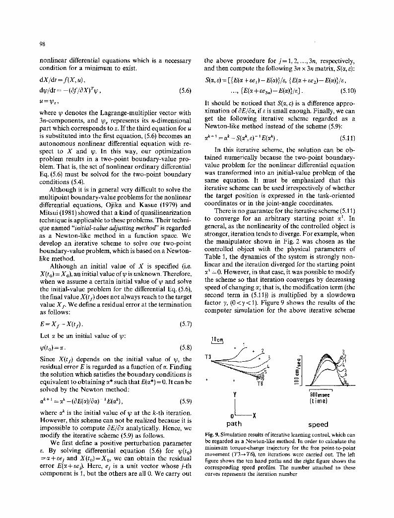
There is no guarantee for the iterative scheme (5.11) to converge for an arbitrary starting point al. In general, as the nonlinearity of the controlled object is stronger, iteration tends to diverge. For example, when the manipulator shown in Fig. 2 was chosen as the controlled object with the physical parameters of Table 1, the dynamics of the system is strongly non- linear and the iteration diverged for the starting point al = 0. However, in that case, it was possible to modify the scheme so that iteration converges by decreasing speed of changing a; that is, the modification term (the second term in (5.11)) is multiplied by a slowdown factor 7, (0<7 < 1). Figure 9 shows the results of the computer simulation for the above iterative scheme

,lOcm 1

+ / " - + 2 ]

r !

Y 500msec

0 X (time)

path speed Fig. 9. Simulation results of iterative learning control, which can be regarded as a Newton-like method. In order to calculate the minimum torque-change trajectory for the free point-to-point movement (T3---}T6), ten iterations were carried out. The left figure shows the ten hand paths and the right figure shows the corresponding speed profiles. The number attached to these curves represents the iteration number

99

setting 7 = 0.4. In this case, the optimal trajectory was almost perfectly realized by the tenth iteration.

The above iterative scheme is applicable to the trajectory planning and control of industrial manipu- lators. In this application, it is an essential problem how to solve the complex nonlinear differential Eq. (5.6). As shown in appendix, its approximate solution can be obtained only by moving the manipu- lator and measuring the trajectories repetitively. In this iterative learning control, the optimum trajectory is directly calculated while neither explicity calculations of inverse kinematics (i.e. coordinates transformation) nor inverse dynamics is necessary. In other words, this algorithm corresponds to step 5 in Fig. 1, in which the three computational problems (trajectory determin- ation, coordinates transformation and generation of motor command) are simultaneously solved by this algorithm. Consequently, this method is very appeal- ing from an engineering point of view.

6 Discussion

We proposed the minimum torque-change model, in some sense, by expanding the minimum jerk model from the viewpoint emphasizing the dynamics of the controlled object.

Recently, Flash (1987) proposed combination of the minimum jerk model with the "equilibrium trajec- tory hypothesis" which was based on the spring-like behavior of the human arm. According to the equilib- rium trajectory hypothesis, the CNS defines the time history of the hand equilibrium positions determined by the neuromuscular activity; hence, the sprink-like force is exerted on the arm according to the difference between the actual and equilibrium hand positions. Flash reported that the equilibrium trajectory hypo- thesis successfully captured both the qualitative fea- tures and the quantitative kinematic details of the measured movements. Flash further discussed that the minimum jerk description might fit the hand equilib- rium trajectories better than the actual trajectories.

We now reconsider these mathematical models and hypothesis from the viewpoint of the computational theory shown in Fig. 1. If one accepts the minimum jerk model or the equilibrium trajectory hypothesis, it also implies that the three computational problems shown in Fig. 1 are solved step by step; that is, the desired trajectory is first planned in terms of the motion of the hand in extracorporal space (step 1), the hand motion is second transformed into the joint motion of the musculoskeletal system of the arm (step 2), and finally, corresponding torque and force are generated so as to realize the desired trajectory (step 3). On the other hand, in the minimum torque- change model, the three problems are simultaneously

solved, and hence planning and execution processes cannot be explicitly separated; that is, the CNS calculates the optimal torque directly as indicated by step 5 in Fig. 1.

In conclusion, the difference between these models is summarized as follows. The minimum jerk model and the equilibrium trajectory hypothesis imply that the motor system is divided between higher levels (e.g., the CNS) and lower levels (e.g., neuromuscular system); in the higher levels, the desired trajectory is planned independently of the musculoskeletal dy- namics; in the lower levels, the associated torque and force are generated. The minimum torque-change model implies that the optimal motor commands (torques and forces) are directly obtained from the dynamics of the musculoskeletal system.

As seen from Fig. 3B, trajectories measured in the planar point-to-point movements were approximately straight but they were not completely straight. Further, hand trajectories were evidently curved for large planar point-to-point movements as shown in Fig. 4B. Two contrary interpretations are considered for these experimental results. One interpretation is that the planned trajectory is straight but the actual trajectory is not straight because of the incomplete control. Another interpretation is that the motion is planned and controlled in accordance with the dynamics of the musculoskeletal system; in other words, the planned trajectory is not straight originally. The equilibrium trajectory hypothesis is compatible with the former interpretation. Our minimum torque change model takes the standpoint of the latter interpretation. The fact that the minimum torque-change model depends heavily on the dynamics of the musculoskeletal system plays an important role to predict the trajectory for the movement affected by the external force (e.g., spring force). According to the minimum torque-change model, the planned trajectory which is the same as the realized trajectory was quite different from that of no load movement as shown in Fig. 6A. It may be possible to explain the constrained movement shown in Fig. 6B by means of the equilibrium trajectory hypothesis. However, it is doubtful whether the equilibrium trajec- tory hypothesis could reproduce the experimental features in the via-point movement shown in Fig. 5B.

As described in previous sections, the minimum torque-change model succeeded in predicting and reproducing very skilled arm movements. However, we do not intend to totally deny the possibility that the CNS performs the step-by=step process (i.e. step 1 ~ 2

3) for some kinds of voluntary arm movements. It is possible to suppose that the CNS performs several kinds of computational schemes (1 ~ 2 ~ 3 , 1 ~4, 5 in Fig. 1) according to different types of voluntary move- ments. When a certain unskilled movement is intended

100

for the first time, the CNS determines the desired trajectory in the visual coordinates, transforms the coordinates and calculates the associated motor com- mand; that is, the CNS performs the step-by-step process ( 1 ~ 2 ~ 3 in Fig. 1) at first. However, we suppose that in the course while the movements is repeatedly executed, a scheme based on the minimum torque-change criterion is gradually acquired. We will propose a neural network model, which learns the energy to be minimized, for this process in our next paper. This scheme corresponds to step 5 in Fig. 1. Hence, for skilled movements such as simple motion between two targets, the optimal trajectory and the associated torque are automatically calculated with- out step 1, 2, and 3, using the scheme acquired by the learning process.

The minimum torque-change model successfully reproduces the observed trajectories under the various conditions (e.g. planar free movement, via-point move- ment and constrained movement under the external force) from the single criterion function Cr. We now consider physiological or physical advantages of mini- mizing C~.. One possible answer might be a mechanical reason. Since the control which minimizes change of torque generates the smooth torque and trajectory, such control reduces wear and tear on the musculo- skeletal system. Furthermore, in that control, the consumption of energy is relatively low (though it is not minimum) because unnecessary force is avoided. Another explanation might be found in inherent dynamics of neural networks in the CNS. This expla- nation is closely related to our neural network model which produces the minimum torque-change trajec- tory, and it will be explained briefly.

Though our iterative scheme is useful to calculate the optimal trajectory with a computer, the CNS does not seem to adopt such an iterative learning scheme based on a Newton-like method. We know that some neural networks can solve computationally difficult problems such as the traveling salesman problem or early visions, which can be regarded as nonlinear optimization problems with some constraints, by minimizing some cost function (energy) (Hopfield 1982; Hopfield and Tank 1985; Poggio et al. 1985; Koch et al. 1986). Because of the success of the minimum torque-change model, the problem of tra- jectory formation for particular types of movements can also be regarded as a nonlinear optimization problem with a constraint given as nonlinear dy- namics of the controlled object.

We recently found a multi-layer neural network model which can generate the minimum torque- change trajectory. This network performs two kinds of parallel information processing: learning process and optimization process. In the learning process, an

internal dynamics model of the controlled object (e.g. arm or manipulator) is acquired by adjusting weights of synaptic connections in the network. During this phase, in some sense, the network learns the energy to be minimized. In the optimization process, using the acquired internal dynamics model, the motor com- mand which minimizes the cost function (energy) is calculated as a result of endogenous dynamics of the neural network. In this way, the minimum torque- change model, if it is reconsidered at the hardware level of Marr, might not so severely contradicts with the neural network model proposed by Bullock and Grossberg (1988), which does not explicitly compute any criterion function.

The minimum torque-change model presented in this paper succeeded in predicting the trajectories of planar two-joint arm movements. It is our future work to investigate whether our model is applicable to other types of movements. In particular, redundant multi- joint movements and obstacle-avoidance movements are interesting. Fortunately, our iterative learning scheme is applicable to these movements.

Acknowledgements. We would like to thank to Mr. Nobuo Fukuda in our laboratory for his technical assistance in the experiments.

Appendix In this appendix, we give the method to solve the Euler-Lagrange Eq. (5.6) indirectly by moving the manipulator and measuring its trajectory repetitively. Let us rewrite (5.6):

dX/dt = f(x, u), (A. 1)

d~0/dt = - (~ f / aX) r~ , (A.2)

u=~pz. (A.3)

The solution X(t) of differential Eq. (A.1) can be obtained from the measured trajectory by moving the manipulator under the control u(t). Furthermore, differential Eq. (A.2) can also be solved indirectly as follows.

If we set 6u(t)- 0 (that is, u(t) is fixed), the variational equation of (A.1) is expressed as

d(rX)/dt = (Of /dX)~SX. (A.4)

Since (A.2) and (A.4) are adjoint with each other, it follows that

dOprrX)/dt=O. (A.5)

Consequently,

~prbs = const. (A.6)

Let gXJ(t) be the solution of variational Eq. (A.4) for JXJ(to) = ej where ej is the j-th unit vector. 6xJ(t) is approximately equal to the variation obtained by measuring the trajectory when only j-th component of X(to) is perturbed. Hence, ~)XJ(t) (j = 1, 2 .... ,3n) are obtained as follows. (Note that X and lp are 3n dimensional vectors, respectively). We first define positive per- turbation parameters e i, (0<ej< 1). X(t) is the trajectory for a given control u(t). Next, we change the initial value of X into

X(to) + ejej,

101

and then we measure the trajectory XJ(t) for the same control u(t). Finally, we get 6XJ(t) from X(t) and XJ(t) as follows;

6X~( t )_~(XJ( t ) - X(t ) ) /e j . (A.7)

Changing the perturbed component of X(to) and performing the above procedure, we get 3n different solutions of (A.4):

6 X l, (~X 2 . . . . , f iX an .

Now, let us define 3n • 3n matrix, D x as follows:

DX = ( ~ X 1 , 6 X 2 . . . . . (~xan). (A.8)

D x is regarded as a fundamental solution matrix of (A.4). From equation (A.6) and definition (A.8), we can easily see that

lp(t)rDx(t) = ~P(to)rDx(to), (t o < t < t l ) . (A.9)

Furthermore, it is clear that

Dx(to) = I ,

where ! represents a unit matrix. Therefore, (A.9) turns out to be

D x ( t f f ~ ( t ) = ~(to). (A. 10)

As seen from the above discussion, when ~(to) is given, the solution of differential Eq. (A.2) can be obtained from (A.10). It should be noticed that we must move the manipulator and measure its trajectory 3n+ 1 times repetitively until we get the solution ~p(t) of (A.2).

References

Abend W, Bizzi E, Morasso P (1982) Human arm trajectory formation. Brain 105:331-348

Atkeson CG, Hollerbach JM (1985) Kinematic features of unrestrained vertical arm movements. J Neurosci 5:2318-2330

Bizzi E, Accornero N, Chapple W, Hogan N (1984) Posture control and trajectory formation during arm movement. J Neurosci 4:2738-2744

Bryson AE, Ho YC (1975) Applied optimal control, Wiley, New York

Bullock D, Grossberg S (1988) Neural dynamics of planned arm movements: Emergent invariants and speed-accuracy pro- perties during trajectory formation. Psychol Rev 95:49-90

Cannon SC, Zahalak GI (1982) The mechanical behavior of active human skeletal muscle in small oscillations. J Biomech 15:111-121

Flash T (1987) The control of hand equilibrium trajectories in multi-joint arm movements. Biol Cybern 57:257-274

Flash T, Hogan N (1985) The coordination of arm movements: An experimentally confirmed mathematical model. J. Neuro- sci 5:1688-1703

Hasan Z (1986) Optimized movement trajectories and joint stiffness in unperturbed, inertially loaded movements. Biol Cybern 53:373-382

Hogan N (1984) An organizing principle for a class of voluntary movements. J Neurosci 4:2745-2754

Hollerbach JM, Flash T (1982) Dynamic interactions between limb segments during planar arm movement. Biol Cybern 44:66-77

Hopfield JJ (1982) Neural networks and physical systems with emergent collective computational abilities. Proe Natl Acad Sci USA 79:2554 2558

Hopfield J J, Tank DW (1985) "Neural" computation of decisions in optimization problems. Biol Cybern 52:141-152

Kawato M, Furukawa K, Suzuki R (1987) A hierarchical neural- network model for control and learning of voluntary move- ment. Biol Cybern 57:169-185

Kawato M, Uno Y, Isobe M, Suzuki R (1988a) A hierarchical neural network model for voluntary movement with appli- cation to robotics. IEEE Control Sys Mag 8:8-16

Kawato M, Isobe M, Maeda Y, Suzuki R (1988b) Coordinates transformation and learning control for visually-guided voluntary movement with iteration: A Newton-like method in a function space. Biol Cybern 59:161-177

Koch C, Marroquin J, Yuille A (1986) Analog "neuronal" networks in early vision. Proc Natl Acad Sci USA 83:4263-4267

Marr D (1982) Vision. Freeman, New York Mitsui T (1981) Newton method for the boundary-value pro-

blems of the differential equations (in Japanese). Math Sci 218:41-46

Morasso P (1981) Spatial control of arm movements. Exp Brain Res 42:223-227

Nelson WL (1983) Physical principles for economies of skilled movements. Biol Cybern 46:135-147

Ojika T, Kasue Y (1979) Initial-value adjusting method for the solution of nonlinear multipoint boundary-value problems. J Math Anal Appl 69:359-371

Poggio T, Torre V, Koch C (1985) Computational vision and regularization theory. Nature 317:314-319

Polite A, Bizzi E (1979) Characteristics of the motor programs underlying arm movements in monkeys. J Neurophysiol 42:183-194

Uno Y, Kawato M, Suzuki R (1987) Formation of optimum trajectory in control of arm movement minimum torque- change model Japan IEICE Technical Report, MBE86-79, 9-16

Received: December 22, 1988

Dr. Yoji Uno Department of Mathematical Engineering and Information Physics Faculty of Engineering University of Tokyo Hongo, Bunkyo-ku Tokyo, 113 Japan