Formalizing Complex Plane Geometry - ARGOargo.matf.bg.ac.rs/publications/2014/moebius.pdf · Formalizing Complex Plane Geometry 3 formal justi cation, authors freely switch between

Noname manuscript No.(will be inserted by the editor)

Formalizing Complex Plane Geometry

Filip Maric · Danijela Petrovic

Received: date / Accepted: date

Abstract Deep connections between complex numbers and geometry had beenwell known and carefully studied centuries ago. Fundamental objects that are in-vestigated are the complex plane (usually extended by a single infinite point),its objects (points, lines and circles), and groups of transformations that act onthem (e.g., inversions and Mobius transformations). In this paper, we treat thegeometry of complex numbers formally and present a fully mechanically verifieddevelopment within the theorem prover Isabelle/HOL. Apart from applicationsin formalizing mathematics and in education, this work serves as a ground forformally investigating various non-Euclidean geometries and their intimate con-nections. We discuss different approaches to formalization and discuss the majoradvantages of the more algebraically oriented approach.

Keywords Interactive theorem proving · Complex plane geometry · Mobiustransformations

1 Introduction

Connections between complex numbers and geometry are deep and intimate. Al-though complex numbers have been recognized for more than 450 years, theirgeometric interpretation came only at the end of 18th century in works of Wes-sel, Argand and Gauss [26]. Their most significant applications in geometry weredeveloped by Cauchy, Riemann, Mobius, Beltrami, Poincare and others duringthe 19th-century [26]. Complex numbers present a very suitable apparatus for in-vestigating properties of objects in very different geometries. Geometry has beenstudied analytically since Descartes, and the Cartesian plane (R2) is often used as

This work is partially supported by the Serbian Ministry of Education and Science grantON174021, and Serbian-French Technology Co-Operation grant EGIDE/,,Pavle Savic” 680-00-132/2012-09/12 (“Formalization and automation of geometry”).

Faculty of MathematicsUniversity of BelgradeStudentski Trg 161100 Belgrade, Serbia

2 Filip Maric, Danijela Petrovic

a domain for models of geometry (especially in the Euclidean case). However, re-placing Cartesian by the complex plane gives simpler and more compact formulasthat describe geometric objects, easing the calculations and shedding some newlight on the subject. Therefore, the complex plane or some of its parts (e.g., theunit disc or the upper half plane) are often taken as the domain in which modelsof various geometries (both Euclidean and non-Euclidean ones) are formalized. Itis also an important domain for investigations in modern physics (see, for exam-ple, Penrose and Rindler [28]). Due to its importance, the geometry of complexnumbers has been well described in the literature. There are many textbooks de-scribing the subject in great detail (during our work we have intensively usedthe textbooks written by Needham [26] and Schwerdtfeger [30]). Also, there is aplethora of course material (handouts, notes, slides) available online. However, weare not aware of any existing formalization of this subject. In this paper we presentour fully formal, mechanically-verified exposition of the complex plane geometrywhich is, up to the best of our knowledge, first of this kind.

The need for rigorous justifications of arguments in geometry have been rec-ognized for more than two millennia — Euclid’s ,,Elements” are one of the firstcases of mathematical deduction and form one of the most beautiful and influen-tial works of science in the history of humankind. In the last century, the work ofHilbert [13] and Tarski [29] enriched us with much more precise developments ofsynthetic geometry. In the last several decades, with the advent of theorem proversand interactive proof-assistants, the level of formality and rigor in geometrical rea-soning has been raised to the highest level. Within the formal theorem provingcommunity, it is often advocated that, apart from the pure ,,L’art pour l’art” viewon formalizing classical mathematical results, there are many practical benefits ofthis task (e.g., in mathematical education). We hope that more mathematicianswill adopt this standpoint. The level of rigor has been constantly rising throughoutthe history of mathematics, and we feel that mechanical theorem proving helpsreaching the ultimate ideal of fully rigorous proofs. Formal, mechanically-checkedanalysis of the content usually fills many gaps often present in classical textbooksand makes the authors think much deeper about the subject that is investigated.As it is often the case in formalization of mathematics, our experience in this workshows that there are not many wrong statements in the informal textbooks. Still,in textbooks that we have analyzed we have found some non-trivial statementsthat were erroneous and could not be proved. Even more abundant are the proofsthat are imprecise, contain uncovered cases and miss some highly non-trivial jus-tifications.

The final product of our present work is a well-developed theory of the extendedcomplex plane (given both as a complex projective space and as the Riemannsphere), its objects (circles and lines), and its transformations (Mobius trans-formations). It can serve as a very important building block for further formalinvestigations of models of various geometries (e.g., our motivation for startingthis work was to formalize the properties of Poincare’s disc model of hyperbolicgeometry). Most of the concepts that we have formalized have already been de-scribed in the literature (although there are many details we had to invent sincethey were not described in the literature that we have consulted). However, ourwork required compiling many different sources into a uniform formal presentationand translating everything into a unique language since it was originally describedin many different ways. For example, even within the same textbook, without any

Formalizing Complex Plane Geometry 3

formal justification, authors freely switch between different settings (e.g., the or-dinary and the extended complex plane), switch between geometric and algebraicexposition, often use many unproved non-trivial facts (regarding them as mathe-matical ,,folklore”), etc. One of our major contributions was clearing this type ofimprecisions and making all the material clear, uniform, and self-contained.

Additionally, we feel that equally (or even more) important to the final resultis our experience gained along the way, during our different attempts to reach ourfinal goal. Namely, there are many different ways in which the subject has beenexposed in the literature. Comparing, for example, Needham [26] and Schwerdt-feger [30], shows two quite different ways of telling the same story — one moregeometrically and the other more algebraically inclined. Our experience shows,that choosing the right approach was the crucial step for making the formalizationmanageable within the proof assistant — it turned out that more algebraic in itsnature the approach was, it was easier to formalize, much nicer, more flexible andmore robust.

In the paper, for succinctness, we will present only the basic results of ourfinal formalization — the most important definitions and statements. The presentpaper contains only a brief recapitulation of the original formal development andmany properties that have been formally proved are not going to be shown in thepaper. Also, no proofs will be shown nor described, as they are all available in theoriginal Isabelle/HOL proof documents1. In the presentation, we will mostly usethe original Isabelle/HOL notation, simplifying it a bit in some places to make itmore approachable for a wider audience.

Outline of the paper. In Subsection 1.1 we discuss some relevant related work. InSection 2 we describe some features of the theorem prover Isabelle/HOL and de-scribe some background theories used in our formalization. Section 3 is the centralsection and contains main results of our formalization — in Subsection 3.1 weintroduce the extended complex plane, in Subsection 3.2 we introduce Mobiustransformations, in Subsection 3.3 we introduce generalized circles, in Subsection3.4 we discuss circle orientation, and in Subsection 3.5 we discuss some importantsubgroups of Mobius transformations. In Section 4 we discuss different approachesthat we have taken in our formalization, their problems and advantages. Finally,in Section 5 we draw conclusions and discuss some potential further work.

1.1 Related Work

During the last decade, there have been many results in formalizing geometry inproof-assistants. Parts of Hilberts seminal book ,,Foundations of Geometry” [13]have been formalized both in Coq and Isabelle/Isar. Formalization of first twogroups of axioms in Coq, in an intuitionistic setting was done by Dehlinger et al.[3]. First formalization in Isabelle/HOL was done by Fleuriot and Meikele [23],and some further developments were made in master thesis of Scott [31]. Largefragments of Tarski’s geometry [29] have been formalized in Coq by Narboux et al.[25]. Within Coq, there are also formalizations of von Platos constructive geometry

1 Isabelle theory files and proof documents are available at http://argo.matf.bg.ac.rs/formalizations/


by Kahn [33,17], French high school geometry by Guilhot [8], ruler and compassgeometry by Duprat [4], projective geometry by Magaud et al. [19], etc.

In our previous work [22,21], we have already formally investigated a Carte-sian model of Euclidean geometry. Timothy Makarios has shown independence ofTarski’s Euclidean axiom by formalizing models of Tarski’s Euclidean and Tarski’snon-Euclidean geometries (the Klein-Beltrami model) [20]. Within that work, thereal projective plane has been formalized in Isabelle/HOL.

As a part of the Flyspeck project, Harrison developed a very rich theory (thatincludes algebra, topology and analysis) of Euclidean n-dimensional space Rn intheorem prover HOL Light [10,12].

Some automated theorem provers in geometry have also been integrated withproof assistants. For example, Janicic et al. describe a detailed formalization (in-cluding implementation details) of the area method [16]. Connecting algebraicmethods (Grobner bases and Wu’s methods) with Coq has been done by Gregoireet al. [7] and by Geneveaux et al. [5].

Different results in complex analysis have also been shown in theorem provers.Milewski has proved the fundamental theorem of algebra in Mizar [24], Geuvers etal. have proved the same theorem in Coq [6], Harrison has implemented complexquantifier elimination in HOL and used it in different formalizations, includinggeometry, etc.

2 Background

In this subsection, we will introduce the theorem prover Isabelle/HOL used forour formalization, its background logic, and notation. We will also briefly describesome results that are part of our formalization, but more general in nature (somelemmas about complex numbers, and the theory of linear algebra of the space C2).

2.1 Isabelle/HOL

Isabelle [27] is a generic proof assistant, but its most developed application is higherorder logic (Isabelle/HOL). Formalizations of mathematical theories are made bydefining new notions (types, constants, functions, etc.), and proving statementsabout them (lemmas, theorems, etc.). This is often done using the declarativeproof language Isabelle/Isar [34]. Isar is a very rich language, and we will heredescribe only the syntax of constructions used in this paper. Definitions are madeusing the syntax definition x where "x = ...", where x is the constant beingdefined. Lemmas are specified using the syntax lemma assumes assms shows

concl where assms are assumptions and concl is the conclusion of the lemma. Ifthere are no assumptions, the keyword shows can be omitted. We will also usethe syntax lemma "

∧x1, . . . xk. Jasm1; ...; asmnK =⇒ concl" where asm1, . . . ,

asmn are the assumptions, concl is the conclusion, and x1, . . . , xk are universallyquantified variables.

Logic formulas are written in the HOL logic using the standard notation (e.g.,the connectives ∧, ∨, −→, ¬, quantifiers ∀ and ∃). Terms can use let-bindings (e.g.,let x = 3 in 3 ∗ x) and if-then-else expressions (e.g., if x > 0 then x else −x),with the standard semantics.


HOL is a typed logic. To express that x is of some type τ we write x :: τ .The predefined type bool denotes Booleans, nat denotes natural numbers, int de-notes integers, real denotes real numbers, while the type complex denotes complexnumbers. The imaginary unit is denoted by ii. All these types support ordinaryarithmetic operations (e.g., +, −, ∗, /). Conversion from real to complex numberwill denoted by cor, the real and imaginary parts of a complex number by Re andIm, the complex conjugate by cnj, the module of a complex number by | |, andthe argument by arg (in Isabelle/HOL it is always in the interval (−π, π]). Thecomplex sign function sgn computes the complex number on the unit circle thathas the same argument as the given non-zero complex number (i.e., sgn z = z/|z|).This function is overloaded and it also applies to real numbers (that overloadingis mathematically justified as for all real x it holds that sgn (x+ ii ∗ 0) = sgn x).The function cis applied to α computes cos α + ii∗sin α.

The type of sets containing elements of the type τ is denoted by τ set. Is-abelle/HOL set-theoretic notation is close to that of standard mathematics, witha few minor exceptions. Set difference is written as X − Y , and the image of afunction f over a set X is written as f ‘X. The product type is denoted by τ1× τ2.Function type is denoted as τ1 ⇒ τ2. Functions are usually curried and functionapplications are written in prefix form, common to functional programming, as f x

(instead of f(x), that is closer to standard mathematical notation). The predicateinj denotes that the function is injective, bij that it is a bijection. The predicatecontinuous on X f denotes that the given function f is continuous on the givenset X. We consider only metric spaces and once we prove that the domain and theco-domain types of f are metric spaces for some distance functions (i.e., that theyinstantiate the metric space type class2), all applications of the continuous on

predicate implicitly assume those distance functions and their induced topologies.New types can be introduced in several ways. The simplest way is to use the

type synonym command that just introduces a new name for an existing type.Another way is by using type definitions and then a new type is specified

to be isomorphic to some non-empty subset of an existing type. For example, atype can be introduced as typedef three = "{0::nat, 1, 2}", generating a proofobligation to show that the type is non-empty. Bijection between the new ab-stract type and its representation type is given by two functions: Rep three ::

three ⇒ nat, and Abs three :: nat ⇒ three, satisfying Rep three x ∈ {0, 1, 2},Rep three (Abs three x) = x, and y ∈ {0, 1, 2} =⇒ Abs three (Rep three y) =

y. In the rest of the paper, representation functions will be denoted by usingb c brackets, and abstraction functions by using d e brackets. The lifting/transferpackage [15] can simplify working with types introduced by typedef. In that case,users usually need not explicitly use the representation and abstraction functions.

Another way to introduce new types, often used in mathematics, are the quo-tient types. In Isabelle/HOL, there are several packages that facilitate workingwith quotients, and our formalization uses the lifting/transfer package [15]. Firststep in defining quotient type is defining an equivalence relation ≈ over some exist-ing (representation) type τ . Quotient type κ is then defined by quotient type κ =

2 Haskell-like type classes [9] are convenient Isabelle/HOL mechanisms for organizing spec-ifications. We say that a type instantiates a type class if there are one on more functionsdefined on that type that satisfy the assumptions required by that type class. For example,metric space type class requires a distance function (metric) satisfying the standard metricaxioms.


τ / ≈. Functions over the quotient type are defined in two steps. First, a functionfτ :: ... τ ... is defined over the representation type τ . Then, that function islifted to the quotient type by using lift definition fκ :: ... κ ... is fτ . Thisgenerates a proof obligation to show that the definition does not depend on thechoice of representative. More details can be found in the literature [18,15].

2.2 Some Background Theories

Complex numbers. Although Isabelle/HOL has some basic support for complexnumbers, it was not sufficient for our needs, so we had to make some significanteffort and extend it. We have proved many lemmas that are very technical and notinteresting for a high-level formalization description so we will not mention them inthis paper (e.g., lemma "arg i = pi/2" or lemma "|z|2 = Re (z ∗ cnj z)"). Oneof the most useful definitions in this section is the definition of angle canonization

function � �, that takes into account 2π periodicity of sine and cosine and mapsany angle to its canonical value that lies within the interval (−π, π]. With thisfunction, for example, multiplicative properties of the arg function can be easilyexpressed and proved.

lemma "z1 ∗ z2 6= 0 =⇒ arg(z1 ∗ z2) = �arg z1 + arg z2�"

Since complex numbers are often treated as vectors, introducing the scalar product

between two complex numbers (it has been defined as 〈z1, z2〉 = (z1 ∗ cnj z2 + z2 ∗cnj z1)/2) showed out to be useful to succinctly express some conditions.

Linear algebra. Next important theory for further formalization is the theory oflinear algebra of C2. Representing vectors and matrices of arbitrary dimensionspose a challenge in HOL, because of lack of dependent types [10]. There are someavailable formalizations of n-dimensional matrices and vectors (e.g., the one in-cluded in the Isabelle/HOL library or the one available on Archive of FormalProofs [32]), but none of these includes the notions that we need (e.g., eigenval-ues, congruence, diagonalization). In our current formalization and its foreseenextensions we only need to consider finite dimension spaces C2 and in some sit-uations R3. Therefore, we have only formalized some linear algebraic propertiesof these small dimensional spaces. Complex vectors (C2 vec) are defined as pairs ofcomplex numbers. Similarly, complex matrices (C2 mat) are defined as 4-tuples of

complex numbers (matrix

(A B

C D

)is represented by (A,B,C,D)). Matrix addition

is denoted by +, subtraction by −, scalar multiplication of vectors is denoted by ∗sv,and matrices by ∗sm. Both vectors and matrices form vector spaces under theseoperations. Scalar product of two vectors is denoted by ∗vv, the product of vector

and matrix by ∗vm, the product of matrix and a vector by ∗mv, and the product of

two matrices by ∗mm. Both zero vector and zero matrix are denoted by 0, identity

matrix is denoted by by eye, the determinant of a matrix is denoted by mat det, itstrace (the sum of diagonal elements) by mat trace, the inverse matrix by mat inv,transpose by mat transpose, conjugation of every vector element by vec cnj, con-

jugation of every matrix element by mat cnj, etc. Regular matrices form a groupunder multiplication. Many standard notions of linear algebra have been intro-duced. For example, eigenvalues and eigenvectors are defined and characterized inthe following way.


definition eigenval :: "complex ⇒ C2 mat ⇒ bool" where

"eigenval k A ←→ (∃v. v 6= 0 ∧ A ∗mv v = k ∗sv v)"lemma "eigenval k A ←→ k2 − mat trace A ∗ k + mat det A = 0"

The adjoint of a matrix is its conjugate transpose. Hermitian matrices are theones equal to their adjoint, while unitary matrices are the ones whose inverse isequal to their adjoint.

definition mat adj where "mat adj H = mat cnj (mat transpose H)"

definition hermitian where "hermitian H ←→ mat adj H = H"

definition unitary where "unitary M ←→ mat adj M ∗mm M = eye"

Other background notions needed in this paper are going to be introducedalong the way, and we refer the reader to our original proof documents for moredetails.

3 Main Results

3.1 Extended Complex Plane

A very important step in developing the geometry of the complex plane is extend-ing the plane C with an additional element (treated as the infinite point). Theextended plane will be denoted by C. There are several different approaches [26,30] to define C. The most appealing approach computationally is the based onhomogeneous coordinates, and the most appealing approach visually is based onthe stereographic projection of the Riemann sphere.

3.1.1 CP 1 — Homogeneous Coordinates

The extended complex plane C is identified with a complex projective line (the one-dimensional projective space over the complex field, sometimes denoted by CP 1).Each point of C is represented by a pair of complex homogeneous coordinates (notboth equal to zero). Two pairs of homogeneous coordinates represent the samepoint in C iff they are proportional by a non-zero complex factor. Isabelle/HOLformalization of this concept relies on the lifting/transfer package for quotients[15] and is done in three stages3.

First, the type of non-zero pairs of complex numbers (also treated as non-zerocomplex vectors) is introduced.

typedef C2 vec6=0 = "{v::C2 vec. v 6= 0}"

This gives the representation function Rep C2 vec6=0 (that we will denote by b cC2)returning a (non-zero) pair of complex numbers for each given element of theauxiliary type C2 vec6=0 and the abstraction function Abs C2 vec6=0 (that we willdenote by d eC2) returning an element of C2 vec6=0 for each given non-zero pair ofcomplex numbers.

Second, two elements of the type C2 vec6=0 are said to be equivalent iff theirrepresentations are proportional.

3 One stage could be avoided by using partial quotients offered by the lifting/transfer pack-age. This feature has not been used in our formalization due to some problems in the earlyversions of the quotient package. All problems have been fixed in the meantime, but our for-malization was quite developed, and it would be quite tedious to change it.


definition ≈C2 :: "C2 vec6=0 ⇒ C2 vec6=0 ⇒ bool" where

"z1 ≈C2 z2 ←→ (∃ (k::complex). k 6= 0 ∧ bz2cC2 = k ∗sv bz1cC2)"

It is quite easy to show that ≈C2 is an equivalence relation.Finally, the type of extended complex numbers given by homogeneous coordi-

nates are defined as equivalence classes of ≈C2 and are introduced as the followingquotient type.

quotient type complexhc = C2 vec6=0 / ≈C2

To summarize, on the lowest representation level there is the type of pairs ofcomplex numbers, on the next level there is the type of non-zero complex 2 × 2vectors (represented by the previous type) and on the highest level there is thequotient type inhabited by equivalence classes — dealing with this quotient type(its representation and abstraction) is done behind the scenes, by the lifting andtransfer package [15]. These three layers of abstraction can be confusing for anordinary mathematician who is used to identify them, but they are necessary in aformal setting where each object must have a unique type (for example, it is usualto consider that (1, i) is both a pair of complex numbers, and a non-zero complexvector, but in our formalization (1, i) is a pair of complex numbers, while d(1, i)eC2

is a non-zero complex vector). In the paper we will always use a non-aggressivenotation (b c and d e) for representation and abstraction functions. Just ignoringthese brackets can make the text more approachable and more like the ordinarymathematical texts.

Ordinary and infinite numbers. Each ordinary complex number can be convertedto an extended complex number.

definition of complex rep :: "complex ⇒ C2 vec6=0" where

of complex rep z = d(z, 1)eC2

lift definition of complex :: "complex ⇒ complexhc" is of complex rep

The single point at infinity is defined the following way

definition inf hc rep :: C2 vec6=0 where inf hc rep = d(1, 0)eC2

lift definition ∞hc :: "complexhc" is inf hc rep

It is easily shown that all extended complex numbers are either ∞hc (iff theirsecond homogeneous coordinate is zero) or can be obtained by converting from anordinary complex number (iff their second homogeneous coordinate is not zero).

lemma "z = ∞hc ∨ (∃ x. z = of complex x)"

Notation 0hc, 1hc and ihc is used to denote extended complex counterparts of0, 1, and i.

Arithmetic operations. Arithmetic operations on ordinary complex numbers can beextended to the extended complex plane.

On the lowest, representation level, the addition of (z1, z2) and (w1, w2) isdefined as (z1 ∗ w2 + w1 ∗ z2, z2 ∗ w2), i.e.,

definition plus hc rep :: "C2 vec6=0 ⇒ C2 vec6=0 ⇒ C2 vec6=0"

where "plus hc rep z w = (let (z1, z2) = bzcC2; (w1, w2) = bwcC2

in d(z1 ∗ w2 + w1 ∗ z2, z2 ∗ w2)eC2)"


This gives a non-zero pair of homogeneous coordinates unless both z2 and w2

are zero (corresponding to the sum of two infinite values), otherwise, it gives anill-defined element d(0, 0)eC2.4 The definition is lifted to the quotient type.

lift definition +hc :: "complexhc ⇒ complexhc ⇒ complexhc" is plus hc rep

This generates the proof obligation Jz ≈C2 z′;w ≈C2 w

′K =⇒ z+hcw ≈C2 z′+hcw

′,that is easily proved by case analysis on whether both z2 and w2 are zero. Notethat, due to the requirement of HOL that all functions are total, we could notdefine the function only for the well-defined cases, and in the lifting proofs we alsohad to deal with the ill-defined cases.

Next, it is shown that this operation extends the ordinary addition of complexnumbers (the operation + on C).

lemma "of complex z +hc of complex w = of complex (z + w)"

The sum of an ordinary complex number and ∞hc is ∞hc (however, ∞hc +hc∞hc

is ill-defined).

lemma "of complex z +hc ∞hc = ∞hc"

lemma "∞hc +hc of complex z = ∞hc"

The operation +hc is associative and commutative, but ∞hc does not have aninverse, so +hc on C does not have the nice algebraic properties of + on C.

Other arithmetic operations are also extended to C. On the lowest, represen-tation type, the unary minus of (z1, z2) is (−z1, z2), the multiple of (z1, z2) and(w1, w2) is (z1 ∗ z2, w1 ∗ w2), and the reciprocal of (z1, z2) is (z2, z1) – these opera-tions are then lifted to the abstract quotient type yielding the operations denotedby uminushc, ∗hc, and reciphc. Subtraction (denoted by −hc) is defined by using+hc and uminushc, and division (denoted by :hc) by using ∗hc and reciphc. Asin the case of addition, it is shown that all these operations match the ordinaryoperations on the finite part of the extended complex plane (e.g. lemma uminushc(of complex z) = of complex (−z)). Next lemmas show the behavior of these op-eration when the infinite point is involved (note that the expressions 0hc ∗hc∞hc,∞hc ∗hc 0hc, 0hc :hc 0hc, and ∞hc :hc ∞hc are ill-defined).

lemma "uminushc ∞hc = ∞hc"

lemma "reciphc ∞hc = 0hc" "reciphc 0hc = ∞hc"

lemma "z 6= 0hc =⇒ z ∗hc ∞hc = ∞hc ∧ ∞hc ∗hc z = ∞hc"

lemma "z 6= 0hc =⇒ z :hc ∞hc = 0hc"lemma "z 6=∞hc =⇒ ∞hc :hc z = ∞hc"

Complex conjugation is also extended to C (on the representation type (z1, z2)is mapped to (z1, z2)), giving the operation cnjhc. A very important operation incomplex geometry is the inversion over the unit circle:

4 All the functions (including the abstraction function d eC2) in HOL are total. However,all the provided lemmas about that function include the precondition that its argument isnot (0, 0). Therefore, there is no way to reason about the value d(0, 0)eC2 and it should be

considered to be ill-defined. The sum ∞hc +hc ∞hc cannot be defined so that C becomes agroup under addition — the law −a + a = 0 requires that ∞hc +hc ∞hc = 0hc (since theopposite element of ∞hc must be ∞hc), but that would break the associativity since then itholds that (∞hc +hc∞hc) +hc 1hc = 1hc 6= 0hc =∞hc +hc (∞hc +hc 1hc).


definition inversionhc :: "complexhc ⇒ complexhc" where

"inversionhc = cnjhc ◦ reciphc"

The most basic properties of inversion are then easily proved.

lemma "inversionhc ◦ inversionhc = id"

lemma "inversionhc 0hc = ∞hc" "inversionhc ∞hc = 0hc"

Ratio and cross ratio. The (simple) ratio and the cross-ratio are very importantconcepts in projective geometry and the extended complex plane (cross-ratio is acharacterizing invariant of Mobius transformations – the fundamental transforma-tions of C, and it is possible to define lines using ratio and circles using cross-ratioof points).

Ratio of points z, v and w is usually defined as z−vz−w . Our definition introduces

it in homogeneous coordinates.

definition ratio rep where "ratio rep z v w =

(let (z1, z2) = bzcC2; (v1, v2) = bvcC2; (w1, w2) = bwcC2

in d((z1 ∗ v2 − v1 ∗ z2) ∗ w2, (z1 ∗ w2 − w1 ∗ z2) ∗ v2)eC2)"

lift definition ratio :: "complexhc ⇒ complexhc ⇒ complexhc ⇒ complexhc"

is ratio rep

Note that this is well-defined in all cases except when z = w = v or z = v =∞hc orz = w =∞hc or v = w =∞hc (however, in the lifting proofs these ill-defined casesmust also be covered). The original ratio of differences is defined in all cases exceptwhen z = w = v or z = ∞hc or v = w = ∞hc, so our definition in homogeneouscoordinates naturally extends the original definition. Following lemmas show thebehavior of the ratio in all well-defined cases (it matches the original ratio ofdifferences whenever it is defined).

lemma "Jz 6= v ∨ z 6= w; z 6=∞hc; v 6=∞hc ∨ w 6=∞hcK =⇒ratio z v w = (z −hc v) :hc (z −hc w)"

lemma Jv 6=∞hc; w 6=∞hcK =⇒ ratio ∞hc v w = 1hclemma Jz 6=∞hc; w 6=∞hcK =⇒ ratio z ∞hc w = ∞hc

lemma Jz 6=∞hc; v 6=∞hcK =⇒ ratio z v ∞hc = 0hc

The last two lemmas are consequences of the first one. Also, note that the ratiocannot be defined for the case when at least two points are infinite in a naturalway (so that the ratio function remains continuous in all of its parameters).

The cross-ratio is defined over 4 points (z, u, v, w), usually as (z−u)(v−w)(z−w)(v−u) . Again,

we define it using homogeneous coordinates.

definition cross ratio rep where "cross ratio rep z u v w =

(let (z1, z2) = bzcC2; (u1, u2) = bucC2;

(v1, v2) = bvcC2; (w1, w2) = bwcC2 in

d(z1 ∗ u2 − u1 ∗ z2) ∗ (v1 ∗ w2 − w1 ∗ v2), (z1 ∗ w2 − w1 ∗ z2) ∗ (v1 ∗ u2 − u1 ∗ v2))eC2"

lift definition cross ratio :: "complexhc ⇒ complexhc ⇒complexhc ⇒ complexhc ⇒ complexhc" is cross ratio rep

This is well-defined in all cases except when z = u = w or z = v = w orz = u = v or u = v = w (note that infinite values for z, u, v or w are allowed,which is not the case in the original fractional formulation). Some basic propertiesof the cross-ratio are given by the following lemmas.


lemma "J(z 6= u ∧ v 6= w) ∨ (z 6= w ∧ u 6= v);z 6=∞hc;u 6=∞hc;v 6=∞hc;w 6=∞hcK=⇒ cross ratio z u v w = ((z −hc u) ∗hc (v−hc) :hc ((z −hc w) ∗hc (v −hc u))"

lemma "cross ratio z 0hc 1hc ∞hc = z"

lemma "J z1 6= z2;z1 6= z3 K =⇒ cross ratio z1 z1 z2 z3 = 0hc"lemma "J z2 6= z1;z2 6= z3 K =⇒ cross ratio z2 z1 z2 z3 = 1hc"lemma "J z3 6= z1;z3 6= z2 K =⇒ cross ratio z3 z1 z2 z3 = ∞hc"

3.1.2 Riemann Sphere and Stereographic Projection

The extended complex plane can be identified with a Riemann (unit) sphere Σ bymeans of stereographic projection [26,30]. The sphere is projected from its northpole N to the xOy plane (identified with C). This projection establishes a bijectivemap sp between Σ\N and the finite complex plane C. The infinite point is definedas the image of N .

In Isabelle/HOL, the sphere Σ is defined as a new type.

typedef riemann sphere = "{(x, y, z)::R3 vec. x2 + y2 + z2 = 1}"

Again, this defines functions Rep riemann sphere (that will be denoted by b cR3

and Abs riemann sphere (that will be denoted by d eR3) that connect the pointsof the abstract type (riemann sphere) and the representation type (triples of realnumbers). Stereographic projection is introduced in the following way:

definition stereographic rep :: "riemann sphere ⇒ C2 vec6=0" where

"stereographic rep M =

(let (x, y, z) = bMcR3

in if (x, y, z) 6= (0, 0, 1) then d(x+ i ∗ y, 1− z)eC2 else d(1, 0)eC2)"

lift definition stereographic :: "riemann sphere ⇒ complexhc" is

stereographic rep

For all points, this is well-defined (the vector (x + i ∗ y, 1 − z) is non-zero as(x, y, z) 6= (0, 0, 1), and (1, 0) is clearly non-zero).

Inverse stereographic projection is defined in the following way.

definition inv stereographic rep :: "C2 vec6=0 ⇒ riemann sphere" where

"inv stereographic rep z =

(let (z1, z2) = bzcC2

in if z2 = 0 then d(0, 0, 1)eR3

else let z = z1/z2; XY = 2 ∗ z / cor (1 + |z|2); Z = (|z|2 − 1)/(1 + |z|2)in d(Re XY, Im XY, Z)eR3)"

lift definition inv stereographic :: "complexhc ⇒ riemann sphere" is

inv stereographic rep

For all points this is well-defined (the sum of squares of three coordinates is 1 inboth cases so the Abs riemann sphere function can safely be applied).

The connection between the two functions is given by the following lemmas.

lemma "stereographic ◦ inv stereographic = id"

lemma "inv stereographic ◦ stereographic = id"

lemma "bij stereographic" "bij inv stereographic"

The proofs are not difficult but require formalizing some tedious calculations.


Chordal distance. Riemann sphere can be made a metric space. One of the mostcommon ways to introduce metric is chordal metric – distance between two pointson the sphere is the length of the chord that joins them.

definition distrs :: "riemann sphere ⇒ riemann sphere ⇒ real" where

"distrs M1 M2 = (let (x1, y1, z1) = bM1cR3; (x2, y2, z2) = bM2cR3

in norm (x1 − x2, y1 − y2, z1 − z2))"

The function norm is a Isabelle/HOL library function and in this case it com-putes the Euclidean vector norm in R3. Using the (already available) fact thatR3 is a metric space (under the distance function λ x y. norm(x − y)), it was notdifficult to show that the type riemann sphere equipped with distrs is a metricspace, i.e., an instantiation of the metric space type class.

Although it is defined on the sphere, the chordal metric has its representationin the plane.

lemma assumes

"stereographic M1 = of complex m1" "stereographic M2 = of complex m2"

shows "distrs M1 M2 = 2 ∗ |m1 −m2| / ( sqrt (1 + |m1|2) ∗ sqrt (1 + |m2|2) )"lemma assumes "stereographic M1 = ∞hs" "stereographic M2 = of complex m"

shows "distrs M1 M2 = 2 / sqrt (1 + |m|2)"lemma assumes "stereographic M1 = of complex m" "stereographic M2 = ∞hs"

shows "distrs M1 M2 = 2 / sqrt (1 + |m|2)"lemma assumes "stereographic M1 = ∞hs" "stereographic M2 = ∞hs"

shows "distrs M1 M2 = 0"

These lemmas make a distinction between finite and infinite points, but thiscase analysis can be avoided if homogeneous coordinates are used.

definition "〈〈z, w〉〉 = (vec cnj bzcC2) ∗vv (bwcC2)"

definition "〈〈z〉〉 = sqrt (Re 〈〈z, z〉〉)"definition "dist hc rep = 2 ∗ sqrt (1− |〈〈z, w〉〉|2/(〈〈z〉〉2 ∗ 〈〈w〉〉2))"lift definition disthc :: "complexhc ⇒ complexhc ⇒ real is dist hc rep

lemma "distrs M1 M2 = disthc (stereographic M1) (stereographic M2)"

This form is sometimes called Fubini-Study metric.The type complexhc equipped with the disthc metric is also an instantiation

of the metric space type class. This trivially follows from the last lemma thatconnects it to the metric space on the Riemann sphere. There are also direct proofsof this (e.g., Hille [14] gives a direct proof due to Shizuo Kakutani, however theproof is incomplete as the possibility of one point being infinite is not considered)and we have formalized them5. It turned out that some properties (e.g., the triangleinequality) are easier to prove on the Riemann sphere using the function distrs,but some properties (e.g., that the metric space is perfect, i.e., that it does nothave isolated points) are easier to prove in the projection using the function disthc,indicating the significance of having different models of the same concept.

Using the chordal metric in the extended plane, and the Euclidean metricon the sphere in R3, the stereographic and inverse stereographic projections areproved to be continuous.

5 Our formalization started without considering the Riemann sphere and so we could onlyuse a direct proof in the beginning, but at one point we introduced the Riemann sphere andusing it explicitly simplified many proofs, including this one.


lemma "continuous on UNIV stereographic"

"continuous on UNIV inv stereographic"

Note that in the previous lemma, metrics are implicit (as described in Section2).

3.2 Mobius Transformations

Mobius transformations (also called homographic, linear fractional, or bilinear trans-formations) are the fundamental transformations of the extended complex plane.In our formalization they are introduced algebraically. Each transformation is rep-resented by a regular (non-singular, non-degenerate) 2×2 matrix that acts linearlyon homogeneous coordinates. As proportional homogeneous coordinates representsame points of C, proportional matrices will represent the same Mobius transfor-mation. Again, the formalization proceeds in three steps using the lifting/transferpackage. First, the type of regular matrices is introduced.

typedef C2 mat reg = "{M :: C2 mat. mat det M 6= 0}"

The representation function Rep C2 mat reg will be denoted by b cM and the ab-straction function Abs C2 mat reg will be denoted by d eM . Regular matrices forma group under multiplication that is usually called general linear group and denotedby GL(2,C). In some cases its subgroup, special linear group, denoted by SL(2,C),and containing only the matrices with the determinant 1 is considered.

Mobius group. Two regular matrices are considered to be equivalent iff their rep-resentations are proportional.

definition ≈M :: "C2 mat reg ⇒ C2 mat reg ⇒ bool" where

"M1 ≈M M2 ←→ (∃ (k::complex). k 6= 0 ∧ bM2cM = k ∗sm bM1cM)"

It is easy to show that this is an equivalence relation. Mobius elements are intro-duced as equivalence classes over this relation.

quotient type mobius = C2 mat reg / ≈M

We will sometimes use the auxiliary constructor mk mobius that returns a Mobiuselement (an equivalence class) for the given 4 complex parameters (it makes senseonly when the corresponding matrix is regular).

Mobius elements form a group under operations that will now define. Thisgroup is called the projective general linear group and denoted by PGL(2,C). Again,SGL(2,C) containing elements with the determinant 1 can be considered. Compo-

sition of Mobius elements is obtained by multiplying their representing matrices.

definition mobius comp rep :: "C2 mat reg ⇒ C2 mat reg ⇒ C2 mat reg"

where "moebius comp rep M1 M2 = dbM1cM ∗mm bM2cMeM"

lift definition mobius comp :: "mobius ⇒ mobius ⇒ mobius" is

mobius comp rep

Similarly, the inverse Mobius element is obtained by taking the inverse representa-tive matrix.


definition mobius inv rep :: "C2 mat reg ⇒ C2 mat reg" where

"mobius inv rep M = dmat inv bMcMeM"

lift definition mobius inv :: "mobius ⇒ mobius" is "mobius inv rep"

Finally, identity Mobius element is represented by the identity matrix.

definition mobius id rep :: "C2 mat reg" where "mobius id rep = deyeeM"

lift definition mobius id :: "mobius" is mobius id rep

All these definitions always introduce well-defined objects (as the product ofregular matrices is regular and the inverse of a regular matrix is regular). Proofobligations necessary to lift the definitions (e.g., M1 ≈M M2 =⇒ mobius inv rep

M1 ≈M mobius inv rep M2) are easily discharged. Composition, inverse and iden-tity establish the group structure on the set of Mobius elements. This is shownby showing that the type mobius along with these operations is an instantiationof the group add type class built-in Isabelle/HOL. Therefore, we will sometimesdenote mobius comp by +, mobius inv by unary −, and mobius id by 0, make sumsof Mobius elements f + g, differences of elements f − g, and so on.

Mobius group action. Action of every Mobius group element on the points of theextended complex plane C induces a mapping from C to C that is a Mobius trans-

formation. The action is given by the function mobius pt.

definition mobius pt rep :: "C2 mat reg ⇒ C2 vec6=0 ⇒ C2 vec6=0"

where "moebius pt rep M z = dbMcM ∗mv bzcC2eC2"

lift definition mobius pt :: "mobius ⇒ complexhc ⇒ complexhc" is

mobius pt rep

Since the product of a regular matrix and a non-zero vector is a non-zero vector, theresult is always well-defined. Lifting the definition generates the obligation JM ≈MM ′; z ≈C2 z′K =⇒ mobius pt rep M z ≈C2 mobius pt rep M ′ z′, that is quiteeasily discharged.

Group operations on Mobius elements correspond to operations on their in-duced Mobius transformations (composition of mappings, inverse mapping andthe identity mapping).

lemma "mobius pt (mobius comp M1 M2) = (mobius pt M1) ◦ (mobius pt M2)"

lemma "mobius pt (mobius inv M) = inv (mobius pt M)"

lemma "mobius pt (mobius id) = id"

The action is transitive (as it is always a bijective map).

lemma "bij (mobius pt M)"

In the classic literature Mobius transformations are often expressed in the formaz+bcz+d , and the following lemma justifies this (but with a special case for the infiniteargument z).

lemma assumes "mat det (a, b, c, d) 6= 0"shows "moebius pt (mk mobius a b c d) z =

(if z 6= ∞hc then

((of complex a) ∗hc z +hc (of complex b)) :hc((of complex c) ∗hc z +hc (of complex d))

else (of complex a) :hc (of complex c))"


An arbitrary transformation of C is a Mobius transformation iff it is an actionof some Mobius group element.

definition is mobius :: "(complexhc ⇒ complexhc) ⇒ bool" where

"is mobius f ←→ (∃ M. f = mobius pt M)"

Note that most results listed so far depend on the fact that the representationmatrix of the Mobius transformation is regular — otherwise, the action would bedegenerate and crush the whole plane C into a single point.

Some special Mobius transformations. Many transformations encountered in geom-etry are special kinds of Mobius transformations. Very important subgroup is thegroup of Euclidean similarities (also called integral transformations). They are deter-mined by using two complex parameters (and represent Mobius transformationswhen the first one is not zero).

definition similarity :: "complex ⇒ complex ⇒ mobius" where

"similarity a b = mk mobius a b 0 1"

Similarities form a group (that is sometimes called the parabolic group).

lemma "Ja 6= 0; c 6= 0K =⇒ mobius comp (similarity a b) (similarity c d) =

similarity (a ∗ c) (a ∗ d+ b)"lemma "a 6= 0 =⇒ mobius inv (similarity a b) = similarity (1/a) (−b/a)"lemma "id mobius = similarity 1 0"

Their action is a linear transformation of C, and each non-constant lineartransformation of C is the action of an element of the similarity group.

lemma "a 6= 0 =⇒ mobius pt (similarity a b) =

(λ z. (of complex a) ∗hc z +hc (of complex b))"

Euclidean similarities are the only Mobius group elements such that their actionleaves the ∞hc fixed.

lemma "mobius pt M ∞hc = ∞hc ←→ (∃ a b. a 6= 0 ∧ M = similarity a b)"

If both∞hc and 0hc are fixed, then its a similarity with coefficients a and b = 0,and the action is of the form λ z. (of complex a) ∗hc z.

lemma "mobius pt M ∞hc = ∞hc ∧ mobius pt M 0hc = 0hc ←→(∃ a. a 6= 0 ∧ M = similarity a 0)"

Euclidean similarities include translations, rotations, and dilatations, and everyEuclidean similarity can be decomposed using these.

definition "translation v = similarity 1 v"

definition "rotation φ = similarity (cis φ) 0"definition "dilatation k = similarity (cor k) 0"lemma "a 6= 0 =⇒ similarity a b =

(translation b) + (rotation (arg a)) + (dilatation |a|)"

Reciprocal (1hc :hc z) is also a Mobius transformation.

definition "reciprocation = mk mobius (1, 0, 0, 1)"lemma "reciphc = mobius pt reciprocation"


On the other hand, inversion is not a Mobius transformation (it is a canonicalexample of so-called anti-Mobius transformations, or antihomographies).

A very important fact is that every Mobius transformation can be composedof Euclidean similarities and a reciprocation. One possible way to achieve thisis given by the following lemma (the case when c = 0 is the case of Euclideansimilarities, and it has already been analyzed).

lemma assumes "c 6= 0" and "a ∗ d− b ∗ c 6= 0"shows "mk mobius a b c d =

translation (a/c) + rotation dilatation ((b ∗ c− a ∗ d)/(c ∗ c)) +

reciprocal + translation (d/c)"

Decomposition is used in many proofs. Namely, to show that every Mobius trans-formation has some property, it suffices to show that reciprocation and all Eu-clidean similarities have that property, and that the property is preserved undercompositions (usually, most of the effort goes to proving the reciprocation case,while the rest is much simpler).

lemma assumes "∧

v. P (translation v)" "∧

α. P (rotation α)""∧

k. P (dilatation k)" "P (reciprocation)""∧

M1 M2. J P M1; P M2 K =⇒ P (M1 +M2)"shows "P M"

Cross-ratio as a Mobius transformation For any fixed three points z1, z2 and z3,cross ratio z z1 z2 z3 can be seen as a function of a single variable z. The fol-lowing lemma guarantees that this function is a Mobius transformation, and bythe properties of the cross-ratio it maps z1 to 0hc, z2 to 1hc and z3 to ∞hc.

lemma "J z1 6= z2; z1 6= z3; z2 6= z3 K =⇒is mobius (λ z. cross ratio z z1 z2 z3)"

Then, the cross-ratio can be used to show that there is a Mobius transformationmapping any three different points to 0hc, 1hc and∞hc, respectively. Since Mobiustransformations form a group, a simple consequence of this is that there is a Mobiustransformation mapping any three different points to any three different points.

lemma "J z1 6= z2; z1 6= z3; z2 6= z3 K =⇒ (∃ M. mobius pt M z1 = 0hc ∧mobius pt M z2 = 1hc ∧ mobius pt M z3 = ∞hc)"

The next lemma turns out to have very important applications in further proofdevelopment, as it enables so-called ,,without-loss-of-generality (wlog)” reasoning[11]. Namely, if the property is preserved under Mobius transformations, theninstead of showing that the property holds for any three different points one canonly show that the property holds for points 0hc, 1hc, and ∞hc.

lemma assumes "P 0hc 1hc ∞hc" "z1 6= z2" "z1 6= z3" "z2 6= z3"

"∧

M u v w. P u v w =⇒P (mobius pt M u) (mobius pt M v) (mobius pt M w)"

shows "P z1 z2 z3"


One of the first applications of ,,wlog” reasoning for Mobius is in analyzingfixed points of Mobius transformations. It is easy to show that only the identitytransformation has the fixed points 0hc, 1hc, and∞hc. It also holds that if a Mobiustransformation M has three different fixed points, it is the identity transformation.The direct proof of this relies on the fact that a 2 × 2 matrix has at most twoindependent eigenvectors, and that can be easily avoided using ,,wlog” reasoning(as any three different points can be mapped to 0hc, 1hc, and ∞hc by some M ′

and then M ′ +M −M ′ has these three points fixed so it must be 0).

lemma "J mobius pt M 0hs = 0hs; mobius pt M 1hs = 1hs;mobius pt M ∞hs = ∞hs K =⇒ M = id mobius"

lemma "J mobius pt M z1 = z1; mobius pt M z2 = z2;

mobius pt M z3 = z3; z1 6= z2; z1 6= z3; z2 6= z3 K =⇒ M = id mobius"

A consequence of this is that there is a unique Mobius transformation mappingthree different points to other three different points (it has already been shownthat there exists such transformation and if there were two, then their differencewould have three different fixed points so it would be identity).

lemma "Jz1 6= z2; z1 6= z3; z2 6= z3; w1 6= w2; w1 6= w3; w2 6= w3K =⇒ ∃! M.

mobius pt M z1 = w1 ∧ mobius pt M z2 = w2 ∧ mobius pt M z3 = w3"

Mobius transformations preserve cross-ratio. Again, a direct proof would becomplicated, so an elegant indirect proof has been formalized (basically, the dif-ference of λz. cross ratio z z1 z2 z3 and M maps (M z1) to 0hc, (M z2) to 1hc,and (M z3) to ∞hc, therefore it must be equal to λz. cross ratio z (M z1) (M

z2) (M z3), and the statement follows by substituting (M z) for z).

lemma "Jz1 6= z2; z1 6= z3; z2 6= z3K =⇒cross ratio z z1 z2 z3 = cross ratio (mobius pt M z) (mobius pt M z1)

(mobius pt M z2) (mobius pt M z3)"

3.3 Circlines

A very important property of the extended complex plane is that it is possibleto treat circles and lines in a uniform way. The basic object is generalized circle,or circline for short. In our formalization, we follow the approach described bySchwerdtfeger [30] and represent circlines by Hermitian, non-zero 2 × 2 matrices.

In the original formulation, a matrix

(A B

C D

)corresponds to the equation A ∗ z ∗

cnj z + B ∗ cnj z + C ∗ z +D = 0, where C = cnjB and A and D are real (as thematrix is Hermitian). The key insight is that this equation represents a line whenA = 0 or a circle, otherwise.

Again, our formalization proceeds in three stages. First, the type of Hermitian,non-zero matrices is introduced.

definition is C2 mat herm :: "C2 mat ⇒ bool" where

"is C2 mat herm H ←→ hermitian H ∧ H 6= 0"typedef C2 mat herm = "{H :: C2 mat. is C2 mat herm H}"


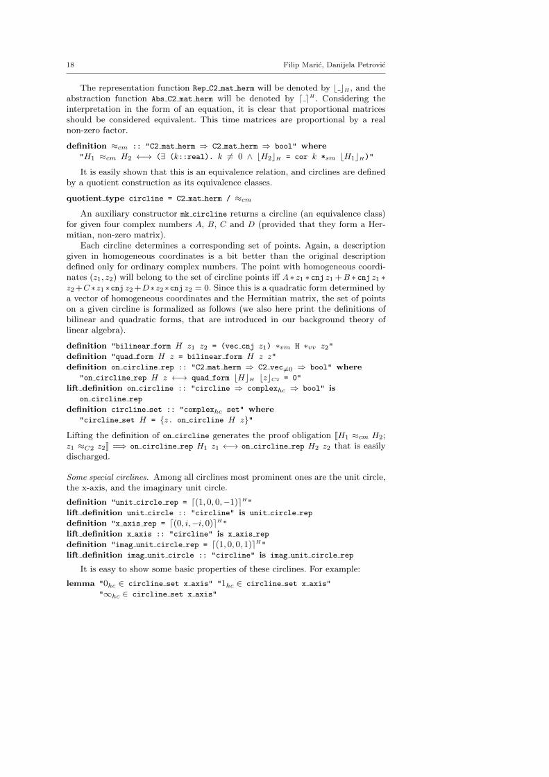
The representation function Rep C2 mat herm will be denoted by b cH , and theabstraction function Abs C2 mat herm will be denoted by d eH . Considering theinterpretation in the form of an equation, it is clear that proportional matricesshould be considered equivalent. This time matrices are proportional by a realnon-zero factor.

definition ≈cm :: "C2 mat herm ⇒ C2 mat herm ⇒ bool" where

"H1 ≈cm H2 ←→ (∃ (k::real). k 6= 0 ∧ bH2cH = cor k *sm bH1cH)"

It is easily shown that this is an equivalence relation, and circlines are definedby a quotient construction as its equivalence classes.

quotient type circline = C2 mat herm / ≈cm

An auxiliary constructor mk circline returns a circline (an equivalence class)for given four complex numbers A, B, C and D (provided that they form a Her-mitian, non-zero matrix).

Each circline determines a corresponding set of points. Again, a descriptiongiven in homogeneous coordinates is a bit better than the original descriptiondefined only for ordinary complex numbers. The point with homogeneous coordi-nates (z1, z2) will belong to the set of circline points iff A ∗ z1 ∗ cnj z1 +B ∗ cnj z1 ∗z2 +C ∗z1 ∗cnj z2 +D∗z2 ∗cnj z2 = 0. Since this is a quadratic form determined bya vector of homogeneous coordinates and the Hermitian matrix, the set of pointson a given circline is formalized as follows (we also here print the definitions ofbilinear and quadratic forms, that are introduced in our background theory oflinear algebra).

definition "bilinear form H z1 z2 = (vec cnj z1) ∗vm H ∗vv z2"

definition "quad form H z = bilinear form H z z"

definition on circline rep :: "C2 mat herm ⇒ C2 vec6=0 ⇒ bool" where

"on circline rep H z ←→ quad form bHcH bzcC2 = 0"

lift definition on circline :: "circline ⇒ complexhc ⇒ bool" is

on circline rep

definition circline set :: "complexhc set" where

"circline set H = {z. on circline H z}"

Lifting the definition of on circline generates the proof obligation JH1 ≈cm H2;z1 ≈C2 z2K =⇒ on circline rep H1 z1 ←→ on circline rep H2 z2 that is easilydischarged.

Some special circlines. Among all circlines most prominent ones are the unit circle,the x-axis, and the imaginary unit circle.

definition "unit circle rep = d(1, 0, 0,−1)eH"lift definition unit circle :: "circline" is unit circle rep

definition "x axis rep = d(0, i,−i, 0)eH"lift definition x axis :: "circline" is x axis rep

definition "imag unit circle rep = d(1, 0, 0, 1)eH"lift definition imag unit circle :: "circline" is imag unit circle rep

It is easy to show some basic properties of these circlines. For example:

lemma "0hc ∈ circline set x axis" "1hc ∈ circline set x axis"

"∞hc ∈ circline set x axis"


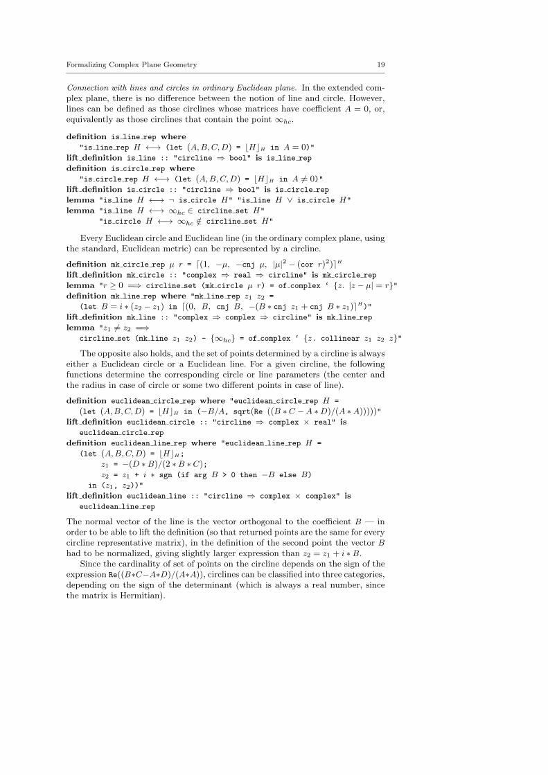
Connection with lines and circles in ordinary Euclidean plane. In the extended com-plex plane, there is no difference between the notion of line and circle. However,lines can be defined as those circlines whose matrices have coefficient A = 0, or,equivalently as those circlines that contain the point ∞hc.

definition is line rep where

"is line rep H ←→ (let (A,B,C,D) = bHcH in A = 0)"lift definition is line :: "circline ⇒ bool" is is line rep

definition is circle rep where

"is circle rep H ←→ (let (A,B,C,D) = bHcH in A 6= 0)"lift definition is circle :: "circline ⇒ bool" is is circle rep

lemma "is line H ←→ ¬ is circle H" "is line H ∨ is circle H"

lemma "is line H ←→ ∞hc ∈ circline set H"

"is circle H ←→ ∞hc /∈ circline set H"

Every Euclidean circle and Euclidean line (in the ordinary complex plane, usingthe standard, Euclidean metric) can be represented by a circline.

definition mk circle rep µ r = d(1, −µ, −cnj µ, |µ|2 − (cor r)2)eHlift definition mk circle :: "complex ⇒ real ⇒ circline" is mk circle rep

lemma "r ≥ 0 =⇒ circline set (mk circle µ r) = of complex ‘ {z. |z − µ| = r}"definition mk line rep where "mk line rep z1 z2 =

(let B = i ∗ (z2 − z1) in d(0, B, cnj B, −(B ∗ cnj z1 + cnj B ∗ z1)eH)"lift definition mk line :: "complex ⇒ complex ⇒ circline" is mk line rep

lemma "z1 6= z2 =⇒circline set (mk line z1 z2) - {∞hc} = of complex ‘ {z. collinear z1 z2 z}"

The opposite also holds, and the set of points determined by a circline is alwayseither a Euclidean circle or a Euclidean line. For a given circline, the followingfunctions determine the corresponding circle or line parameters (the center andthe radius in case of circle or some two different points in case of line).

definition euclidean circle rep where "euclidean circle rep H =

(let (A,B,C,D) = bHcH in (−B/A, sqrt(Re ((B ∗ C −A ∗D)/(A ∗A)))))"lift definition euclidean circle :: "circline ⇒ complex × real" is

euclidean circle rep

definition euclidean line rep where "euclidean line rep H =

(let (A,B,C,D) = bHcH;z1 = −(D ∗B)/(2 ∗B ∗ C);z2 = z1 + i ∗ sgn (if arg B > 0 then −B else B)

in (z1, z2))"

lift definition euclidean line :: "circline ⇒ complex × complex" is

euclidean line rep

The normal vector of the line is the vector orthogonal to the coefficient B — inorder to be able to lift the definition (so that returned points are the same for everycircline representative matrix), in the definition of the second point the vector Bhad to be normalized, giving slightly larger expression than z2 = z1 + i ∗B.

Since the cardinality of set of points on the circline depends on the sign of theexpression Re((B∗C−A∗D)/(A∗A)), circlines can be classified into three categories,depending on the sign of the determinant (which is always a real number, sincethe matrix is Hermitian).


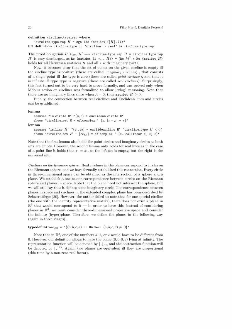
definition circline type rep where

"circline type rep H = sgn (Re (mat det (bHcH)))"lift definition circline type :: "circline ⇒ real" is circline type rep

The proof obligation H ≈cm H ′ =⇒ circline type rep H = circline type rep

H ′ is easy discharged, as Re (mat det (k ∗sm H)) = (Re k)2 ∗ Re (mat det H)

holds for all Hermitian matrices H and all k with imaginary part 0.Now, it becomes clear that the set of points on the given circline is empty iff

the circline type is positive (these are called imaginary circlines) , that consistsof a single point iff the type is zero (these are called point circlines), and that itis infinite iff type type is negative (these are called real circlines). Surprisingly,this fact turned out to be very hard to prove formally, and was proved only whenMobius action on circlines was formalized to allow ,,wlog” reasoning. Note thatthere are no imaginary lines since when A = 0, then mat det H ≥ 0.

Finally, the connection between real circlines and Euclidean lines and circlescan be established.

lemma

assumes "is circle H" "(µ, r) = euclidean circle H"

shows "circline set H = of complex ‘ {z. |z − µ| = r}"lemma

assumes "is line H" "(z1, z2) = euclidean line H" "circline type H < 0"shows "circline set H - {∞hc} = of complex ‘ {z. collinear z1 z2 z}"

Note that the first lemma also holds for point circles and imaginary circles as bothsets are empty. However, the second lemma only holds for real lines as in the caseof a point line it holds that z1 = z2, so the left set is empty, but the right is theuniversal set.

Circlines on the Riemann sphere. Real circlines in the plane correspond to circles onthe Riemann sphere, and we have formally established this connection. Every circlein three-dimensional space can be obtained as the intersection of a sphere and aplane. We establish a one-to-one correspondence between circles on the Riemannsphere and planes in space. Note that the plane need not intersect the sphere, butwe will still say that it defines some imaginary circle. The correspondence betweenplanes in space and circlines in the extended complex plane has been described bySchwerdtfeger [30]. However, the author failed to note that for one special circline(the one with the identity representative matrix), there does not exist a plane inR3 that would correspond to it — in order to have this, instead of consideringplanes in R3, we must consider three-dimensional projective space and considerthe infinite (hyper)plane. Therefore, we define the planes in the following way(again in three stages).

typedef R4 vec6=0 = "{(a, b, c, d) :: R4 vec. (a, b, c, d) 6= 0}"

Note that in R3, one of the numbers a, b, or c would have to be different from0. However, our definition allows to have the plane (0, 0, 0, d) lying at infinity. Therepresentation function will be denoted by b cR4, and the abstraction function willbe denoted by d eR4. Again, two planes are equivalent iff they are proportional(this time by a non-zero real factor).


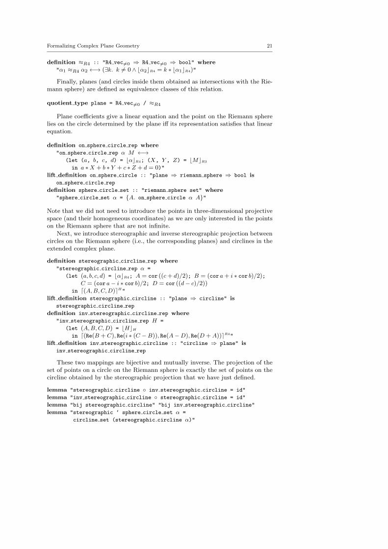
definition ≈R4 :: "R4 vec6=0 ⇒ R4 vec6=0 ⇒ bool" where

"α1 ≈R4 α2 ←→ (∃k. k 6= 0 ∧ bα2cR4 = k ∗ bα1cR4)"

Finally, planes (and circles inside them obtained as intersections with the Rie-mann sphere) are defined as equivalence classes of this relation.

quotient type plane = R4 vec6=0 / ≈R4

Plane coefficients give a linear equation and the point on the Riemann spherelies on the circle determined by the plane iff its representation satisfies that linearequation.

definition on sphere circle rep where

"on sphere circle rep α M ←→(let (a, b, c, d) = bαcR4; (X, Y , Z) = bMcR3

in a ∗X + b ∗ Y + c ∗ Z + d = 0)"lift definition on sphere circle :: "plane ⇒ riemann sphere ⇒ bool is

on sphere circle rep

definition sphere circle set :: "riemann sphere set" where

"sphere circle set α = {A. on sphere circle α A}"

Note that we did not need to introduce the points in three-dimensional projectivespace (and their homogeneous coordinates) as we are only interested in the pointson the Riemann sphere that are not infinite.

Next, we introduce stereographic and inverse stereographic projection betweencircles on the Riemann sphere (i.e., the corresponding planes) and circlines in theextended complex plane.

definition stereographic circline rep where

"stereographic circline rep α =

(let (a, b, c, d) = bαcR4; A = cor ((c+ d)/2); B = (cor a+ i ∗ cor b)/2);C = (cor a− i ∗ cor b)/2; D = cor ((d− c)/2))

in d(A,B,C,D)eH"lift definition stereographic circline :: "plane ⇒ circline" is

stereographic circline rep

definition inv stereographic circline rep where

"inv stereographic circline rep H =

(let (A,B,C,D) = bHcHin d(Re(B + C), Re(i ∗ (C −B)), Re(A−D), Re(D +A))eR4"

lift definition inv stereographic circline :: "circline ⇒ plane" is

inv stereographic circline rep

These two mappings are bijective and mutually inverse. The projection of theset of points on a circle on the Riemann sphere is exactly the set of points on thecircline obtained by the stereographic projection that we have just defined.

lemma "stereographic circline ◦ inv stereographic circline = id"

lemma "inv stereographic circline ◦ stereographic circline = id"

lemma "bij stereographic circline" "bij inv stereographic circline"

lemma "stereographic ‘ sphere circle set α =

circline set (stereographic circline α)"


Chordal circlines. Another interesting fact is that real circlines are sets of pointsthat are equidistant from some given points (there are always exactly two of them),but in the chordal metric. On the Riemann sphere these two points (we will callthem chordal centers) are obtained as intersections of the sphere and the line thatgoes through the center of the circle and is normal to the plane that contains thecircle.

A chordal circline determined by the given point a and radius r is determinedin the following way.

definition chordal circle rep where "chordal circle rep µc rc =

(let (µ1, µ2) = bµccC2;

A = 4 ∗ |µ2|2 − (cor rc)2 ∗ (|µ1|2 + |µ2|2); B = −4 ∗ µ1∗cnj µ2;

C = −4∗cnj µ1 ∗ µ2; D = 4 ∗ |µ1|2 − (cor rc)2 ∗ (|µ1|2 + |µ2|2)

in mk circline rep A B C D)"

lift definition chordal circle :: "complexhc ⇒ real ⇒ circline" is

chordal circle rep

lemma "z ∈ circline set (chordal circle µc rc) ←→rc ≥ 0 ∧ disthc z µc = rc"

If a circline is given, then its chordal centers and radii can be determined rely-ing on the following lemmas (depending on whether coefficients B and C in therepresentation matrix are zero).

lemma

assumes "is C2 mat herm (A,B,C,D)" "Re (A ∗D) < 0" "B = 0"shows

"mk circline A B C D = chordal circle ∞hc sqrt(Re ((4 ∗A)/(A−D)))""mk circline A B C D = chordal circle 0hc sqrt(Re ((4 ∗D)/(D −A)))"

lemma assumes

"is C2 mat herm (A,B,C,D)" "Re (mat det (A,B,C,D)) < 0" "B 6= 0""C ∗ µ2c + (D −A) ∗ µc −B = 0" "rc = sqrt((4 + Re((4 ∗ µc/B) ∗A))/(1 + Re(|µc|2)))"shows "mk circline A B C D = chordal circle (of complex µc) rc"

As in the previous cases, the function that returns chordal parameters could beintroduced (it would need to distinguish between the cases of B = 0 and B 6= 0 andin the other case to solve the quadratic equation describing the chordal center).

Symmetry. Since ancient Greeks, the circle inversion was seen as a counterpart ofline reflection. In the extended complex plane there are no substantial differencesbetween circles and lines. Therefore, we will consider only one kind of relation andcall two points circline symmetric if they are mapped to one another using eitherreflection or inversion over arbitrary line or circle. When, seeking the algebraiccharacterization of this relation we were a bit surprised how simple and elegantit was – points are symmetric iff the bilinear form of their representation vectorsand matrix is zero.

definition circline symmetric rep where

"circline symmetric rep z1 z2 H ←→ bilinear form bz1cC2 bz2cC2 bHcH = 0"lift definition circline symmetric :: "complexhc ⇒ complexhc ⇒

circline ⇒ bool" is circline symmetric rep


Returning to the set of points on the circline and comparing our two definitions,it becomes clear that points on the circline are exactly those that are invariantunder the symmetry of the circline.

lemma "on circline H z ←→ circline symmetric H z z"

Mobius action on circlines. We have already seen that Mobius transformation acton the points of C. They can also act on circlines (and the definition is chosen sothat the two actions are compatible). We also print the definition of congruenceoperation of two matrices (defined in our background theory of linear-algebra).

definition "congruence M H = mat adj M ∗mm H ∗mm M"

definition mobius circline rep

:: "C2 mat reg ⇒ C2 mat herm ⇒ C2 mat herm" where

"mobius circline rep M H = dcongruence (mat inv bMcM) bHcHeH"lift definition mobius circline :: "mobius ⇒ circline ⇒ circline" is

mobius circline rep

Mobius actions on circlines have similar properties as Mobius actions on points.For example,

lemma "mobius circline (mobius comp M1 M2) =

mobius circline M1 ◦ mobius circline M2"

lemma "mobius circline (mobius inv M) = inv (mobius circline M)"

lemma "mobius circline (mobius id) = id"

lemma "inj mobius circline"

The central lemma in this section connects the action of Mobius transforma-tions on points and on circlines (and shows that the Mobius transformations mapcirclines to circlines).

lemma "mobius pt M ‘ circline set H =

circline set (mobius circline M H)"

Circline type is also preserved (implying, for example, that real circlines aremapped to real circlines).

lemma "circline type (mobius circline M H) = circline type H"

Another important property (a bit more general than the previous one) isthat the symmetry of points is preserved by Mobius transformations (the so-calledsymmetry principle).

lemma assumes "circline symmetric z1 z2 H"

shows "circline symmetric (mobius pt M z1) (mobius pt M z2)

(mobius circline M H)"

The last two lemmas are quite prominent geometrical results, and, due tothe convenient, algebraic representation they were relatively easy to prove in ourformalization. Both proofs rely on the following simple fact of linear algebra.

lemma "mat det M 6= 0 =⇒ "bilinear form z1 z2 H =

bilinear form (M ∗mv z1) (M ∗mv z2) (congruence (mat inv M) H)"


Circline uniqueness. In Euclidean geometry, it is a well-known fact that there is aunique line through any two different points and a unique circle through any threedifferent points. Similar results hold in C. However, a case-analysis over the typeof circlines must be performed. Positive type circlines contain no points, so thereare no uniqueness results for them. Zero type circlines consist of a single point andfor each point there is a unique zero type circline containing it. There is a uniquecircline through any three different points (and it must be of a negative type).

lemma "∃! H. circline type H = 0 ∧ z ∈ circline set H"

lemma "Jz1 6= z2; z1 6= z3; z2 6= z3K =⇒∃! H. z1 ∈ circline set H ∧ z2 ∈ circline set H ∧ z3 ∈ circline set H"

Very surprisingly, we did not manage to prove these lemmas directly. However,employing ,,wlog” reasoning and mapping the points to canonical position (0hc,1hc, and ∞hc) gave us very short and elegant proofs (as it was easy to showcomputationally that the x axis is the only circline through these three points).As lines are characterized as exactly those circlines that contain ∞hc, so it is clearthat there is a unique line through any two finite points.

Circline set cardinality. Another thing usually taken for granted is the cardinality ofcirclines of different type. We have already said that these proofs required ,,wlog”reasoning, but this time we have used ,,wlog” reasoning of a different kind. In manycases it turns out that it is simpler to reason about circles if their center is in theorigin — in those cases, their matrix is diagonal. We have formalized the specialcase of the famous result of linear algebra claiming that each Hermitian 2x2 matrixis congruent to a real diagonal matrix. Moreover, the elements on the diagonal arethe real eigenvalues of the matrix and the congruence is established by a unitarymatrix — a congruence could be also established by a simpler, translation matrix,but then it would not have so nice properties.

lemma assumes "hermitian H"

shows "∃ k1 k2M. mat det M 6= 0 ∧ unitary M ∧congruence M H = (cor k1, 0, 0,cor k2)"

The consequence is that for every circline there is a unitary Mobius transfor-mation that transforms it to a position such that its center is in the origin (in fact,there are two such transformations if eigenvalues are different). We shall see thatunitary transformations correspond to rotations of the Riemann sphere, so thelast fact has a simple geometrical explanation. Circlines could be diagonalized byusing translations only, but unitary transformations often have nicer properties.

lemma "∃ M H ′. unitary mobius M ∧mobius circline M H = H ′ ∧ circline diag H ′"

lemma assumes "∧

H ′. circline diag H ′ =⇒ P H"

"∧

M H. P H =⇒ P (mobius circline M H)"

shows "P H"

The predicate unitary mobius lifts the unitary condition from C2 matrices to themobius type. Similarly, circline diag lifts the diagonal matrix condition to thecircline type.

Using this kind of ,,wlog” reasoning it becomes fairly easy to show the followingcharacterizations of circline set cardinality.


lemma "circline type H > 0 ←→ circline set H = {}"lemma "circline type H = 0 ←→ ∃z. circline set H = {z}"lemma "circline type H < 0 ←→

∃ z1 z2 z3. z1 6= z2 ∧ z1 6= z3 ∧ z2 6= z3 ∧ circline set H ⊇ {z1, z2, z3}"

An important, non-trivial, consequence of the circline uniqueness and the cir-cline set cardinality is that the function circline set is injective, i.e., for eachnon-empty set of points of a circline, there is a unique class of proportional ma-trices determining it.

lemma "J circline set H1 = circline set H2; circline set H1 6= {} K =⇒H1 = H2"

The lemma does not hold for the empty set of points as there are many non-equivalent matrices determining it (each imaginary circline has the empty set ofpoints). Although we could have made the definition of circlines that declare allimaginary circlines to be equivalent, our current definition distinguishes differentimaginary circlines and gives their finer classification. Looking at the Riemannsphere shows that it is very natural to distinguish different imaginary circlinessince they are identified with different planes that do not intersect the sphere.

3.4 Oriented Circlines

In this section we describe how the orientation is introduced for the circlines.Many important concepts depend on the orientation. One of the most importantis the concept of disc — inside area of a circline. Similarly as the set of circlinepoints, the set of disc points is introduced using the quadratic form induced bythe circline matrix — the set of points of the circline disc is the set of points such

that satisfy that A∗ z ∗cnj z+B ∗cnj z+C ∗ z+D < 0, where

(A B

C D

)is a circline

matrix representative. Since the set of disc points must be invariant to the choiceof representative, it is clear that oriented circlines matrices are equivalent onlyif they are proportional by a positive real factor (recall that unoriented circlineallowed arbitrary non-zero real factors).

definition ≈ocm :: "C2 mat herm ⇒ C2 mat herm ⇒ bool" where

"H1 ≈ocm H2 ←→ (∃ (k::real). k > 0 ∧ bH2cH = cor k ∗sm bH1cH)"

It is easily shown that this is an equivalence relation, so circlines are definedby a quotient construction as its equivalence classes.

quotient type o circline = C2 mat herm / ≈ocm

Now we can use the quadratic forms to define the interior, boundary and theexterior of an oriented circline.

definition on o circline rep :: "C2 mat herm ⇒ C2 vec6=0 ⇒ bool" where

"on o circline rep H z ←→ quad form bHcH bzcC2 = 0"

definition in o circline rep :: "C2 mat herm ⇒ C2 vec6=0 ⇒ bool" where

"in o circline rep H z ←→ quad form bHcH bzcC2 < 0"

definition out o circline rep :: "C2 mat herm ⇒ C2 vec6=0 ⇒ bool" where

"out o circline rep H z ←→ quad form bHcH bzcC2 > 0"


These definitions are then lifted to on o circline, in o circline, and out o circline

(proving the necessary obligations), and, finally, the next three definitions are in-troduced.

definition o circline set :: "complexhc set" where

"o circline set H = {z. on o circline H z}"definition disc :: "complexhc set" where

"disc H = {z. in o circline H z}"definition disc compl :: "complexhc set" where

"disc compl H = {z. out o circline H z}"

These three sets are mutually disjoint, and they fill up the entire plane.

lemma "disc H ∩ disc compl H = {}""disc H ∩ o circline set H = {}""disc compl H ∩ o circline set H = {}""disc H ∪ disc compl H ∪ o circline set H = UNIV"

Given an oriented circline, one can trivially obtain its unoriented counterpart,and these two share the same set of points.

lift definition of o circline ( #) :: "o circline ⇒ circline" is id

lemma "circline set (H#) = o circline set H"

Note that in the previous lift definition we have introduced the superscriptnotation for the function of o circline, so, for example, H# in the lemma is ashorthand for of o circline H.

For each circline, there is exactly one opposite oriented circline

definition "opp o circline rep H = d−1 ∗sm bHcHeH"lift definition opp o circline ( ↔) :: "o circline ⇒ o circline" is

opp o circline rep

Finding opposite circline is idempotent, and opposite circlines share the same setof points, but exchange disc and its complement.

lemma "(H↔)↔ = H"

lemma "o circline set (H↔) = o circline set H"

"disc (H↔) = disc compl H" "disc compl (H↔) = disc H"

The functions # and o circline set are injective in some sense.

lemma "H1# = H2

# =⇒ H1 = H2 ∨ H1 = H2↔"

lemma "Jo circline set H1 = o circline set H2; o circline set H1 6= {}K =⇒H1 = H2 ∨ H1 = H2

↔"

Given a representative Hermitian matrix of a circline, it represents exactly oneof the two possible oriented circlines. The choice of what should be called a positiveorientation is arbitrary. We follow Schwerdtfeger [30], use the leading coefficientA as the first criterion, and say that circline matrices with A > 0 are calledpositively oriented, and with A < 0 negatively oriented. However, Schwerdtfegerdid not discuss the possible case of A = 0 (the case of lines), so we had to extendhis definition to achieve a total characterization.


definition "pos o circline rep where "pos o circline rep H ←→(let (A, B, C, D) = bHcH

in Re A > 0 ∨(Re A = 0 ∧ ((B 6= 0 ∧ arg B > 0) ∨ (B = 0 ∧ Re D > 0))))"

lift definition pos o circline :: "o circline ⇒ bool" is pos o circline rep

Now, exactly one of the two oppositely oriented circlines is positively oriented.

lemma "pos o circline H ∨ pos o circline (H↔)"

"pos o circline (H↔) ←→ ¬ pos o circline H"

The orientation of circles is both algebraically simple (the sign of the coefficientA) and geometrically natural, due to the following simple characterization.

lemma "∞h /∈ o circline set H =⇒ pos o circline H ←→ ∞h /∈ disc H"

Another nice geometric characterization of positive orientation is that the posi-tively oriented Euclidean circles contain their Euclidean centers in the disc.

lemma assumes "is circle (H#)" "circline type (H#) < 0"

"(µ, r) = euclidean circle (H#)"

shows "pos oriented H ←→ of complex µ ∈ disc H"

Note that the orientation of lines and point circles is artificially introduced (onlyto have a total positive orientation characterization), and it does not have a nat-ural geometric interpretation. This breaks the continuity of orientation, and wethink that it is not possible to introduce the orientation of lines, so that the orien-tation function becomes everywhere continuous. Therefore, in most lemmas thattell something about the orientation we will explicitly exclude the case of lines.

Having a total characterization for the positive orientation allows to create acoercion from an unoriented to an oriented circline (returning always the positivelyoriented circline).

definition of circline rep :: "C2 mat herm ⇒ C2 mat herm" where

"of circline rep H = (if pos o circline rep H then H

else opp o circline rep H)"

lift definition of circline ( ) :: "circline ⇒ o circline" is of circline rep

There are many elementary properties of the function of circline proved, andhere we list some most important.

lemma "o circline set (H) = circline set H"

lemma "pos o circline (H)"

lemma "(H)#

= H" "pos o circline H =⇒ (H#)

= H"

lemma "H1 = H2

=⇒ H1 = H2"

Mobius action on oriented circlines. On the representation level, the Mobius actionon an oriented circline is the same as on an unoriented circline.

lift definition mobius o circline :: "mobius ⇒ o circline ⇒ o circline" is

mobius circline rep

Mobius action on (unoriented) circlines could have been defined using the actionon oriented circlines, but not the other way around.


lemma "mobius circline M H = (mobius o circline M (H))#"

lemma "let H1 = mobius o circline M H; H2 = (mobius circline M (H#))

in H1 = H2 ∨ H1 = H2↔"

Mobius actions on oriented circlines have similar properties as Mobius actions onunoriented ones. For example, they agree with inverse (lemma "mobius o circline

(mobius inv M) = inv (mobius o circline M)"), with composition, identity trans-formation, they are injective (inj mobius circline), and so on. The central lem-mas in this section connects the action of Mobius transformations on points, onoriented circlines, and discs.

lemma "mobius pt M ‘ o circline set H =

o circline set (mobius o circline M H)"

lemma "mobius pt M ‘ disc H = disc (mobius o circline M H)"

lemma "mobius pt M ‘ disc compl H = disc compl (mobius o circline M H)"

All Euclidean similarities preserve circline orientation.

lemma assumes "a 6= 0" "M = similarity a b" "∞hc /∈ o circline set H"

shows "pos o circline H ←→ pos o circline (mobius o circline M H)"

Orientation of the image of a given oriented circline H under a given Mobiustransformation M depends on whether the pole of M (the point that M maps to∞hc) lies in the disc or in the disc complement of H (if the pole lies on the circlineH, then the circline maps onto a line and we do not discuss the orientation).

lemma

"0hc ∈ disc compl H =⇒ pos o circline (mobius o circline reciprocation H)"

"0hc ∈ disc H =⇒ ¬ pos o circline (mobius o circline reciprocation H)"

lemma

assumes "M = mk mobius a b c d" "c 6= 0" "a ∗ d− b ∗ c 6= 0"shows "pole M ∈ disc H −→ ¬ pos o circline (mobius o circline M H)"

"pole M ∈ disc compl H −→ pos o circline (mobius o circline M H)"

Note that this is different to what is claimed by Schwerdtfeger [30]: ,,Reciproca-tion preserves the orientation of a circle which does not contain 0, but inverts theorientation of any circle containing 0 as an interior point. Every Mobius trans-formation preserves the orientation of any circle that does not contain its pole. Ifcircle contains its pole, then the image circle has its orientation opposite.”. Ourformalization shows that the orientation of the image circle does not depend onthe orientation of the initial one. For example, in the case of reciprocation, theorientation of the initial circle depends only on the sign of the coefficient A ina representation matrix (i.e., on the relationship between the circle disc and theinfinite point). On the other hand, since reciprocation exchanges coefficients A andD, the orientation of the image circle depends only on the sign of the coefficient D(i.e., on the relationship between the initial circle disc and the point zero — thepole of reciprocation). The coefficients A and D are totally independent, so theorientation of the image does not depend on the orientation of the initial circle.

Angle preservation. Mobius transformations are conformal, meaning that they pre-serve oriented angle between oriented circlines. If angle is defined in purely alge-braic terms (following Schwerdtfeger [30]), then this property is a very easy toprove. We also print the definition of a mixed determinant defined in our back-ground theory of linear algebra.


fun mat det mix :: "C2 mat ⇒ C2 mat ⇒ complex" where

"mat det mix (A1, B1, C1, D1) (A2, B2, C2, D2) =

A1 ∗D2 −B1 ∗ C2 +A2 ∗D1 −B2 ∗ C1"

definition cos angle rep where

"cos angle rep H1 H2 = − Re (mat det mix bH1cH bH2cH) /

2 ∗ (sqrt (Re (mat det bH1cH ∗ mat det bH2cH)))"lift definition cos angle :: "o circline ⇒ o circline ⇒ complex" is

cos angle rep

lemma "cos angle H1 H2 =

cos angle (moebius o circline M H1) (moebius o circline M H2)"

However, this definition is not intuitive, and for pedagogical reasons we want toconnect it to the more common definition. First, we define the angle between twocomplex vectors (� � denotes the angle canonization function described earlier).

definition ang vec ("]") where "] z1 z2 = �arg z2 - arg z1�"

Given a center µ of an ordinary Euclidean circle and a point z on it, we definethe tangent vector in z as the radius vector −→µz, rotated by π/2, clockwise orcounterclockwise, depending on the circle orientation.

definition tang vec :: "complex ⇒ complex ⇒ bool ⇒ complex" where

"tang vec µ z p = sgn bool p ∗ i ∗ (z − µ)"

The Boolean p encodes the orientation of the circle, and the function sgn bool p

returns 1 when p is true, and −1 for when p is false. Finally, angle between twooriented circles at their common point z is defined as the angle between tangentvectors at z.

definition ang circ where

"ang circ z µ1 µ2 p1 p2 = ] (tang vec µ1 z p1) (tang vec µ2 z p2)"

Finally, the connection between algebraic and geometric definition of angle cosineis given by the following lemma.

lemma assumes "is circle (H1#)" "is circle (H2

#)"

"circline type (H1#) < 0" "circline type (H2

#) < 0""(µ1, r1) = euclidean circle (H1

#)"

"(µ2, r2) = euclidean circle (H2#)"

"of complex z ∈ o circline set H1 ∩ o circline set H2"

shows "cos angle H1 H2 =

cos (ang circ z µ1 µ2 (pos o circline H1) (pos o circline H2))"

To prove this lemma we needed to show the law of cosines in Isabelle/HOL, butit turned out to be a rather simple task.

3.5 Some Important Subgroups of Mobius Transformations

We have already described the parabolic group (the group of Euclidean similar-ities), crucial for the Euclidean plane geometry. Now we will describe character-izations of two very important subgroups of the Mobius group — the group ofsphere rotations, important for the elliptic plane geometry, and the group of discautomorphisms, important for the hyperbolic plane geometry.


Sphere rotations. General unitary group, denoted by GU2(C) is the group thatcontains all Mobius transformations represented by generalized unitary matrices.

definition unitary gen where

"unitary gen M ←→ (∃ k::complex. k 6= 0 ∧ mat adj M ∗mmM = k ∗sm eye)"

Although the definition allows any complex factor k, it turns out that k can only bereal. Generalized unitary matrices can be factored into ordinary unitary matricesand positive multiples of the identity matrix.

definition unitary where "unitary M ←→ mat adj M ∗mmM = eye"

lemma "unitary gen M ←→(∃ k M ′. k > 0 ∧ unitary M ′ ∧ M = (cor k ∗sm eye) ∗mm M ′)"

The group of unitary matrices is very important as it describes all rotations ofthe Riemann sphere (it is isomorphic to the real special orthogonal group SO3(R)).One characterization of GU2(C) in C is that it is a group of transformations thatleave the imaginary unit circle fixed (this is the circle with the identity represen-tation matrix, contained in the plane at infinity).

lemma "mat det (A,B,C,D) 6= 0 =⇒ unitary gen (A, B, C, D) ←→moebius circline (mk moebius A B C D) imag unit circle =

imag unit circle"

The characterization of generalized unitary matrices in coordinates is given bythe following lemma.

lemma "unitary gen M ←→ (∃ a b k. let M ′ = (a, b, −cnj b, cnj a) in

k 6= 0 ∧ mat det M ′ 6= 0 ∧ M = k ∗smM ′)"

Along the way we have also defined the special unitary group SU2(C), contain-ing generalized unitary matrices with unit determinant. They are recognized bythe form (a, b, −cnj b, cnj a), without the multiple k, and we used this to derivethe coordinate form of generalized unitary matrices.

Disc automorphisms. A dual group to the previous one is the group of generalizedunitary matrices with the 1− 1 signature (GU1,1(C)).

definition unitary11 where

"unitary11 M ←→ mat adj M ∗mm (1, 0, 0,−1) ∗mmM = (1, 0, 0,−1)"definition unitary11 gen where

"unitary11 gen M ←→ (∃ k::complex. k 6= 0 ∧mat adj M ∗mm(1, 0, 0,−1)∗mm M = k ∗sm (1, 0, 0,−1))"

Again, the definition allows a complex factor k, but it is shown that only realfactors are plausible.

A characterization of the GU1,1(C) is that it contains all Mobius transforma-tions that leave the unit circle fixed.

lemma "mat det (A,B,C,D) 6= 0 =⇒ unitary11 gen (A,B,C,D) ←→moebius circline (mk moebius A B C D) unit circle = unit circle"

The characterization of generalized unitary 1-1 matrices in coordinates is givenby the following lemmas.


lemma "unitary11 gen M ←→ (∃ a b k. let M ′ = (a, b, cnj b, cnj a) in

k 6= 0 ∧ mat det M ′ 6= 0 ∧ (M = k ∗smM ′ ∨ M = k ∗sm (cis pi, 0, 0, 1) ∗smM ′))lemma "unitary11 gen M ←→ (∃ a b k. let M ′ = (a, b, cnj b, cnj a) in

k 6= 0 ∧ mat det M ′ 6= 0 ∧ M = k ∗smM ′ )"

Note that the first lemma is subsumed by the second one. However, the first lemmawas simpler to prove, and gives matrices of another shape k∗sm(a, b, −cnj b, −cnj a)— geometrically, the second kind of transformation combines the first kind withan additional central symmetry.

Another important characterization of these transformations is via so-calledBlaschke factors. Each transformation is a composition of a Blaschke factor (areflection that brings some point that is not on the unit circle to zero), and arotation.

lemma assumes "k 6= 0" "M ′ = (a, b, cnj b, cnj a)""M = k ∗smM ′" "mat det M ′ 6= 0" "a 6= 0"

shows "∃ k′ φ a′. k′ 6= 0 ∧ a′ ∗ cnj a′ 6= 1 ∧M = k′ ∗sm (cis φ, 0, 0, 1) ∗mm (1, −a′, −cnj a′, 1)"

The exceptions come when a = 0 and then instead of the Blaschke factor, areciprocation is used (the infinity plays the role of a′ in the previous lemma).

lemma assumes "k 6= 0" "M ′ = (0, b, cnj b, 0)" "b 6= 0" "M = k ∗smM ′"shows "∃ k′ φ. k′ 6= 0 ∧ M = k′ ∗sm (cis φ, 0, 0, 1) ∗mm (0, 1, 1, 0)"

Matrices of GU1,1(C) naturally split into two subgroups. All transformations fixthe unit circle, but the first subgroup consists of transformations that map the unitdisc to itself (so-called disc automorphisms), while the second subgroup consists oftransformations that exchange the unit disc and its complement. Given a matrix,its subgroup can be determined only on by looking at the sign of the determinantof M ′ = (a, b, cnj b, cnj a). If only M = (a1, b1, c1, d1), and not M ′ nor k is given,a criterion to determine the subgroup is the value of sgn(Re ((a1∗d1)/(b1∗c1))−1).

Note that all the important subgroups are here described only in pure algebraicterms. We have also formalized some more geometric proofs resulting in equivalentcharacterization to these we have just described. Additionally, it holds that allanalytic disc automorphisms are compositions of Blaschke factors and rotations(however, the proofs relies on mathematical analysis, maximum modulus principle,and the Swartz lemma — techniques that we did not consider). Even the weakerstatement claiming that all Mobius disc automorphisms are of this form has notyet been formally proved. The crucial step is showing that disc automorphisms fixthe unit circle, and that is something that we did not manage to do without deeptopological investigations that we are currently working on.

4 Discussion

When developing a formal library, an important question is how to define thenotions and formulate their properties so that the proofs become shorter and sothat their large parts can be automated. In this section, we present an examplethat demonstrates how complicated it is to formalize a proof when notions aredefined naively, by following classical mathematical material. Although proofs that


are only semi-formal and that fail to discuss some corner cases are inherentlyproblematic, the problems often become evident only when one tries to formalizethem within a proof assistant. Namely, readers sometimes do not care much aboutcorner cases and are usually satisfied with such proofs because they are simple andintuitive.

In the current example, we will consider one classic definition of angle betweencircles and then analyze one classic proof of the angle preservation property ofMobius transformations that is often encountered in textbooks on the subject(in the rest of this section we will follow Needham [26] which does not aim tobe a very formal book, but, still, that kind of reasoning is common for manyother authors). Comparison to our purely algebraic definition of angle and thecorresponding proof of the angle preservation property given in Section 3.4 revealsthat the classic proof lacks formality and, therefore, it is very hard to formalize itwithin a proof assistant. On the other hand, the classic proof offers more intuitionand better understanding (as it can be visualized).

Angles can be defined between oriented, or unoriented curves and angles them-selves can be oriented or unoriented. Needham defines angles between two curvesin the following way: ,,Let S1 and S2 be curves intersecting at z. As illustrated, we

may draw their tangent lines T1 and T2 at z. The angle between curves S1 and S2 at

their common point z is the acute angle α from T1 to T2. Thus this angle α has a

sign attached to it: the angle between S2 and S1 is minus the illustrated angle between

S1 and S2.” So, the angle is defined only between unoriented curves (and that isdifferent from our definition given in Section 3.4), but the angle itself is oriented(and that is the same as in our definition). We first define the unoriented convexand the acute angle between two vectors.

definition "]c" where "]c z1 z2 ≡ abs (] z1 z2)"definition acutize where "acutize α = (if α > π

2 then π - α else α)"definition "]a" where "]a z1 z2 ≡ acutize (]c z1 z2)"

The function ang circ a is defined as the acute angle between the two tangentvectors of two intersecting circles (it is similar to ang circ, but the returned anglemust always be acute). As our circles are oriented, we have shown that the acuteangle between the two circles is not affected by the orientation and can only beexpressed in terms of three points (the intersection point and the two centers).

lemma "Jz 6= µ1;z 6= µ2K =⇒ ang circ a z µ1 µ2 p1 p2 = ]a (z − µ1) (z − µ2)"

The angle preservation proof for Mobius transformations in the textbook [26]relies on the fact that each Mobius transformation can be decomposed to trans-lations, rotation, dilatation, and inversion. The fact that translations, rotations,and dilatations preserve angles is taken for granted (and, to be honest, formalizingthis was rather simple, once the underlying notions were defined appropriately).Therefore, the central challenge is to show that inversion preserves angles, i.e., that,,inversion in a circle is an anticonformal mapping”. The proof relies on the ,,fact

that given any point z not on the inversion circle K, there is precisely one circle or-

thogonal to K that passes through z in any given direction”. Then the proof proceeds,,Suppose that two curves S1 and S2 intersect at z, and that their tangents there are T1and T2, the angle between them being α. To find out what happens to this angle under

inversion in K, let us replace S1 and S2 with the unique circles R1 and R2 orthogonal


to K that pass through z in the same directions as directions S1 and S2, i.e., circles

whose tangents at z are T1 and T2. Since inversion in K maps each of these circles to

themselves, the new angle at z is −α. Done.”

We have formalized this ,,proof”, but this required tremendous amount of ef-fort, compared to the sleek algebraic proof described in Section 3.4. First, thetextbook is often imprecise in whether it deals with ,,complex inversion” or ,,ge-ometric inversion” (i.e., between the reciprocation and the inversion put in ourterms). In the textbook proof, the author uses inversion over any circle K, butit is sufficient to consider only the reciprocation (always given over the unit cir-cle). Formalizing the textbook reasoning only for the reciprocation already gavequite large formulas, and it would be even more complicated and tedious (if notimpossible) to finish the proof using inversion over arbitrary circle. For example,a simple reciprocation of a circle with a center µ and radius r gives a circle withthe center µ = µ/cor (|µ|2 − r2), and radius r = r/||µ|2 − r2|, and this relationshipwould be much more complex for an arbitrary Mobius transformation, if it waswritten in coordinates, without using matrix notation.

The formal angle preservation statement is the following (circle µ r denotesthe set {z. |z − µ| = r}, µ1, µ2, µ1, µ2, z, z are complex numbers, and r1, r2, r1,and r2 are real numbers).

lemma

assumes "z ∈ circle µ1 r1" "z ∈ circle µ2 r2"

"reciprocation ‘ circle µ1 r1 = circle µ1 r1"

"reciprocation ‘ circle µ2 r2 = circle µ2 r2"

"z ∈ circle µ1 r1" "z ∈ circle µ2 r2"

shows "ang circ a z µ1 µ2 = ang circ a z µ1 µ2"

Apart from missing discussion of many special cases, the informal proof missesone key ingredient. Namely, it is easy to prove that the intersection of R1 and R2

is z (the intersection of S1 and S2, the images of S1 and S2 under inversion), butshowing that R1 and S1 and that R2 and S2 share tangents at z required not sotrivial calculations (that proof relies on the fact that center µ′i of Ri, the center µiof Si, and z are collinear).

Simple symmetry argument showing that the angles between the circles in theirtwo different intersection points are the same was again not so simple to formalize.

lemma assumes "µ1 6= µ2" "r1 > 0" "r2 > 0""{z1, z2} ⊆ circle µ1 r1 ∩ circle µ2 r2" "z1 6= z2"

shows "ang circ a z1 µ1 µ2 = ang circ a z2 µ1 µ2"

We have shown this lemma only after employing ,,wlog” reasoning and moving theconfiguration so that the centers of the two circles are on the x-axis.

In the proof, we have found many degenerate cases that had to be analyzedseparately. First, we had to prove that intersecting circles can share the samecenter (i.e., that µ1 6=µ2) only if they are the same, and then the acute anglebetween tangents is 0. If the two centers are collinear with the intersection pointz (i.e., if collinear µ1 µ2 z holds), the two circles touch (either from inside orfrom the outside), and again the acute angle is 0.

Existence of the circle Ri orthogonal to the unit circle, sharing the same tangentin the given point z with the given circle centered in the given point µi is given


by the following lemma (ortho unit circ denotes the set of points on the circlecentered in µ′i, orthogonal to unit circle).

lemma

assumes "〈µi - z, z〉 6= 0""µ′i = z + (1− z∗cnj z) ∗ (µi − z)/(2 ∗ 〈µi − z, z〉)"

shows "collinear z µi µ′i" "z ∈ ortho unit circ µ′i"

The analytic expressions reveal some other degenerate cases. The numerator of thefraction can be zero only when the circles intersect on the unit circles (i.e., whenz ∗cnj z = 1). In that case, the textbook proof cannot be adapted, as µ′1 = µ′2 = z,and the circles R1 and R2 cannot not be constructed (they are the empty circles).The case when denominator is zero (either for µ′1 or µ′2) is also degenerate. Thathappens when vectors µi− z and z are orthogonal. Geometrically, in that case thecircle Ri degenerates into a line (what is not a problem in the extended complexplane, but is a problem in the original proof set in the ordinary complex plane).Therefore, this special case had to be handled separately. So, our formal analysisquickly shows that the simple statement in Needham that ,,given any point z noton the inversion circle K, there is precisely one circle orthogonal to K that passesthrough z in any given direction” is not true in many cases.

Problems demonstrated in this example occur in many other proofs in the clas-sic literature on the subject, showing that our choice of purely algebraic definitionsin our formalization was an extremely important step to keep the formalizationsimple and the proofs short.

5 Conclusions and Further Work

In this paper, we have described some elements of our formalization of the geometryof the complex plane C both as complex projective line and the Riemann sphere,arithmetic operations in C, ratio and cross-ratio, chordal metric in C, the groupof Mobius transformations and their action on C, some of its special subgroups(Euclidean similarities, sphere rotations, disk automorphisms), circlines and theirconnection with circles and lines, the chordal metric, and the Riemann sphere,Mobius action of circlines, circline uniqueness, circline types and set cardinality,oriented circlines, relations between Mobius transformations and the orientation,angle preservation properties of Mobius transformations, etc. Our current devel-opment counts around 12,000 lines of Isabelle/HOL code (all proofs are structuredand written in the proof language Isabelle/Isar, and our early attempts that aresubsumed by shorter algebraic proofs are not included), around 125 definitionsand around 800 lemmas.

The crucial step in our formalization was our decision to use the algebraicrepresentation of all relevant objects (e.g., vectors of homogeneous coordinates,matrices for Mobius transformations, Hermitian matrices for circlines). Althoughthis is not a new approach (for example, Schwerdtfeger’s classic book [30] followsthis approach quite consistently), it is not so common in the literature (and inthe course material available online). Instead, other, more geometrically orientedapproaches prevail. We have tried to follow that kind of geometric reasoning in ourearly work on this subject, but we have encountered many difficulties and did not


have so much success. Based on this experience, we conclude that introducing thepowerful techniques of linear algebra makes the work on formalization an order ofmagnitude simpler than when using just plain geometric reasoning.

It can be argued that sometimes geometrical arguments give better explana-tions of some theorems, but when only justification is concerned, the algebraicapproach is clearly superior. However, to keep the connection with the standard,geometric intuition, several definitions must be introduced (more geometric, andmore algebraic ones), and they must be proved equivalent. For example, when thedefinition of angles is given only through algebraic operations on matrices and theirdeterminants, the angle preservation property is very easy to prove. However, foreducational purposes this becomes relevant only when that definition is connectedwith the standard definition of angle between curves (i.e., their tangent vectors),or, otherwise, the formalization becomes a game with meaningless symbols.

Another important conclusion that we make is that in formal documents, caseanalysis should be avoided and extensions that help avoiding it should be pursuedwhenever possible (e.g., it was much better to use the homogeneous coordinatesinstead of a single distinguished infinity point, it was much simpler to work withcirclines than to distinguish between circles and lines, etc.). Keeping different mod-els of the same concept (for example, homogeneous coordinates and the Riemannsphere) also helps, as some proofs are easier in one, and some proofs are easier inother models.

In principle, our proofs are not long (15-20 lines in average with each Isar state-ment in a separate line). However, some tedious reasoning was sometimes required,especially when switching between real and complex numbers (by the conversionfunctions Re and cor). These conversions are usually not present in informal texts,and some better automation of reasoning about them would be welcome. Isabelle’sautomation was quite powerful in equational reasoning about ordinary complexnumbers using (simp add: field simps) (with some minor exceptions). However,the automation was not so good in the presence of inequalities and we had tomanually prove many things that would be considered trivial in informal texts.

Since in our formalization quotients are intensively used, porting it to someother prover would require that the prover has good support for them. Introducingthe concepts using quotients is a natural operation in Isabelle/HOL and otherHOL provers, but might pose challenges to other provers. For example, in anintensional type theory it is not always possible to form the quotient of a type byan equivalence relation. In Coq, the problem with quotient types is that there is nogeneral way of forming them, without axioms. One approach considers quotientsof setoids [1] — setoid is a type with an equivalence relation called setiod equalityand quotienting a setiod amounts to changing the setoid equality to a broaderone. A pragmatic approach to quotients in Coq/SSReflect is recently describedby Cohen [2]. Besides quotients, when porting our formalization to other provers,library support for complex numbers, trigonometric functions and abstract algebra(automated reasoning in fields, groups, vector and metric spaces, etc.) would bevery welcome.

In our further work we plan to use these results for formalizing non-Euclideangeometries and their models (especially, spherical model of the elliptic geometryand the Poincare disc and upper half-plane models of hyperbolic geometry). Wealso plan to generalize our linear algebraic results to arbitrary dimensions, as suchlibrary could be useful in other contexts.


Acknowledgements The authors are grateful to Pascal Schreck, Pierre Boutry, Julien Nar-boux, and anonymous reviewers of AMAI journal for many valuable suggestions and advice.

References

1. Gilles Barthe, Venanzio Capretta, and Olivier Pons. Setoids in type theory. Journal ofFunctional Programming, 13(2):261–293, 2003.

2. Cyril Cohen. Pragmatic quotient types in Coq. In Sandrine Blazy, Christine Paulin-Mohring, and David Pichardie, editors, Interactive Theorem Proving, volume 7998 of Lec-ture Notes in Computer Science, pages 213–228. Springer Berlin Heidelberg, 2013.

3. Christophe Dehlinger, Jean-Francois Dufourd, and Pascal Schreck. Higher-Order Intuition-istic Formalization and Proofs in Hilberts Elementary Geometry. In Automated Deductionin Geometry, volume 2061 of Lecture Notes in Computer Science. Springer, 2001.

4. Jean Duprat. Constructors: a ruler and a pair of compasses. In TYPES 2002. 2002.5. Jean-David Genevaux, Julien Narboux, and Pascal Schreck. Formalization of Wu’s simple

method in Coq. In CPP, volume 7086 of Lecture Notes in Computer Science. Springer,2011.

6. Herman Geuvers, Freek Wiedijk, and Jan Zwanenburg. A Constructive Proof of theFundamental Theorem of Algebra without Using the Rationals. In Types for Proofs andPrograms, volume 2277 of Lecture Notes in Computer Science. Springer, 2002.

7. Benjamin Gregoire, Loıc Pottier, and Laurent Thery. Proof certificates for algebra andtheir application to automatic geometry theorem proving. In Automated Deduction inGeometry, volume 6301 of Lecture Notes in Computer Science. Springer, 2008.

8. Frederique Guilhot. Formalisation en Coq et visualisation d’un cours de geometrie pourle lycee. Technique et Science Informatiques, 24(9), 2005.

9. Florian Haftmann and Makarius Wenzel. Constructive type classes in isabelle. In Types forProofs and Programs, volume 4502 of Lecture Notes in Computer Science, pages 160–174.Springer Berlin Heidelberg, 2007.

10. John Harrison. A HOL Theory of Euclidean Space. In TPHOLs, volume 3603 of LectureNotes in Computer Science. Springer, 2005.

11. John Harrison. Without loss of generality. In Proceedings of the 22nd InternationalConference on Theorem Proving in Higher Order Logics, TPHOLs 2009, volume 5674 ofLNCS, Munich, Germany, 2009. Springer-Verlag.

12. John Harrison. The HOL Light Theory of Euclidean Space. J. Autom. Reasoning, 50(2),2013.

13. David Hilbert and E.J. Townsend. The Foundations Of Geometry. Kessinger Publishing,2006.

14. Einar Hille. Analytic Function Theory. AMS Chelsea Publishing. American MathematicalSociety, 1973.

15. Brian Huffman and Ondrej Kuncar. Lifting and Transfer: A Modular Design for Quotientsin Isabelle/HOL. In Certified Programs and Proofs, volume 8307 of LNCS. SpringerInternational Publishing, 2013.

16. Predrag Janicic, Julien Narboux, and Pedro Quaresma. The Area Method. Journal ofAutomated Reasoning, 48(4), 2012.

17. Gilles Kahn. Constructive geometry according to Jan von Plato. Coq contribution, CoqV5.10, 1995.

18. Cezary Kaliszyk and Christian Urban. Quotients revisited for Isabelle/HOL. In Proceed-ings of the 2011 ACM Symposium on Applied Computing, SAC ’11, pages 1639–1644, NewYork, NY, USA, 2011. ACM.

19. Nicolas Magaud, Julien Narboux, and Pascal Schreck. Formalizing Projective Plane ge-ometry in Coq. In Automated Deduction in Geometry, volume 6301 of Lecture Notes inComputer Science. Springer, 2011.

20. Timothy James McKenzie Makarios. A mechanical verification of the independence ofTarski’s Euclidean axiom. Master’s thesis, Victoria University of Wellington, 2012.

21. Filip Maric and Danijela Petrovic. Formalizing analytic geometries. In Automated Deduc-tion in Geometry. 2012.

22. Filip Maric, Ivan Petrovic, Danijela Petrovic, and Predrag Janicic. Formalization andimplementation of algebraic methods in geometry. In THedu, volume 79 of EPTCS, 2011.


23. Laura Meikle and Jacques Fleuriot. Formalizing Hilberts Grundlagen in Isabelle/Isar.In Theorem Proving in Higher Order Logics, volume 2758 of Lecture Notes in ComputerScience. Springer, 2003.

24. Robert Milewski. Fundamental theorem of algebra. Formalized Mathematics, 9(3), 2001.25. Julien Narboux. Mechanical Theorem Proving in Tarski’s Geometry. In Automated De-

duction in Geometry, volume 4869 of Lecture Notes in Computer Science. Springer, 2007.26. Tristan Needham. Visual Complex Analysis. Oxford University Press, 1998.27. Tobias Nipkow, Lawrence C. Paulson, and Markus Wenzel. Isabelle/HOL — A Proof

Assistant for Higher-Order Logic, volume 2283 of LNCS. Springer, 2002.28. Roger Penrose and Wolfgang Rindler. Spinors and Space-Time. Cambridge Monographs

on Mathematical Physics. Cambridge University Press, 1987.29. Wolfram Schwabhauser, Wanda Szmielew, Alfred Tarski, and Michael Beeson. Metamath-

ematische Methoden in der Geometrie. Springer, Verlag, 1983.30. Hans Schwerdtfeger. Geometry of Complex Numbers. Dover Books on Mathematics. Dover

Publications, 1979.31. Phil Scott. Mechanising Hilberts Foundations of Geometry in Isabelle. Master’s thesis,

University of Edinburgh, 2008.32. Christian Sternagel and Rene Thiemann. Executable matrix operations on matrices of

arbitrary dimensions. Archive of Formal Proofs, June 2010. http://afp.sf.net/entries/Matrix.shtml, Formal proof development.

33. Jan von Plato. The axioms of constructive geometry. Annals of Pure and Applied Logic,76(2), 1995.

34. Makarius Wenzel. Isabelle/Isar — a generic framework for human-readable proof docu-ments. In From Insight to Proof — Festschrift in Honour of Andrzej Trybulec, Studiesin Logic, Grammar, and Rhetoric, volume 10(23). University of Bialystok, 2007.

Documents

Formalizing Complex Plane Geometry - ARGOargo.matf.bg.ac.rs/publications/2014/moebius.pdf · Formalizing Complex Plane Geometry 3 formal justi cation, authors freely switch between