Embed Size (px)
Citation preview

Formal modeling and verification of distributed failuredetectorsCitation for published version (APA):Atif, M. (2011). Formal modeling and verification of distributed failure detectors. Technische UniversiteitEindhoven. https://doi.org/10.6100/IR716364
DOI:10.6100/IR716364
Document status and date:Published: 01/01/2011
Document Version:Publisher’s PDF, also known as Version of Record (includes final page, issue and volume numbers)
Please check the document version of this publication:
• A submitted manuscript is the version of the article upon submission and before peer-review. There can beimportant differences between the submitted version and the official published version of record. Peopleinterested in the research are advised to contact the author for the final version of the publication, or visit theDOI to the publisher's website.• The final author version and the galley proof are versions of the publication after peer review.• The final published version features the final layout of the paper including the volume, issue and pagenumbers.Link to publication
General rightsCopyright and moral rights for the publications made accessible in the public portal are retained by the authors and/or other copyright ownersand it is a condition of accessing publications that users recognise and abide by the legal requirements associated with these rights.
• Users may download and print one copy of any publication from the public portal for the purpose of private study or research. • You may not further distribute the material or use it for any profit-making activity or commercial gain • You may freely distribute the URL identifying the publication in the public portal.
If the publication is distributed under the terms of Article 25fa of the Dutch Copyright Act, indicated by the “Taverne” license above, pleasefollow below link for the End User Agreement:www.tue.nl/taverne
Take down policyIf you believe that this document breaches copyright please contact us at:[email protected] details and we will investigate your claim.
Download date: 22. Oct. 2021
Formal Modeling and Verification ofDistributed Failure Detectors
PROEFSCHRIFT
ter verkrijging van de graad van doctoraan de Technische Universiteit Eindhoven, op gezag van de
rector magnificus, prof.dr.ir. C.J. van Duijn, voor eencommissie aangewezen door het College voor
Promoties in het openbaar te verdedigenop woensdag 28 september 2011 om 14.00 uur
door
Muhammad Atif
geboren te Samundri, Pakistan
Dit proefschrift is goedgekeurd door de promotoren:
prof.dr.ir. J.F. Grooteenprof.dr. M.G.J. van den Brand
Copromotor:dr. M.R. Mousavi
A catalogue record is available from the Eindhoven University of Technology LibraryISBN:978-90-386-2620-8
Atif, Muhammad
Formal Modeling and Verification of Distributed Failure Detectors / Muhammad Atif. -Eindhoven : Technische Universiteit Eindhoven, 2011.NUR 992Subject headings: fault-tolerance ; formal methods / analysis ; distributed protocolsCR Subject Classification: B.3.4, B.4.4, C.2.2, C.2.4, D.2.4, D.2.5, D.4.1, F.3.1, F.4.1, I.2.4

Eerste promotor: prof.dr.ir. Jan Friso Groote (Technische Universiteit Eindhoven)
Tweede promotor: prof.dr. Mark van den Brand (Technische Universiteit Eindhoven)
Copromotor: dr. MohammadReza Mousavi (Technische Universiteit Eindhoven)
Kerncommissie:prof.dr. W.J. Fokkink (Vrije Universiteit Amsterdam)dr. I. Ulidowski (University of Leicester)prof.dr.ir. L.M.G. Feijs (Technische Universiteit Eindhoven)
The work in this thesis is supported by Higher Education Commission of Pakistan.The work in this thesis has been carried out under the auspices of the researchschool IPA (Institute for Programming research and Algorithmics). IPA disserta-tion series 2011–10c© Muhammad Atif 2011. All rights are reserved. Reproduction in whole or inpart is prohibited without the written consent of the copyright owner.Printing: Eindhoven University PressCover design: Verspaget & Bruinink
Contents
List of Figures v
0 Preface ix
1 Introduction 11.1 The subject matter . . . . . . . . . . . . . . . . . . . . . . . . . . . 21.2 Models of distributed computation . . . . . . . . . . . . . . . . . . 3
1.2.1 Communication model . . . . . . . . . . . . . . . . . . . . . 31.2.2 Timing model . . . . . . . . . . . . . . . . . . . . . . . . . . 41.2.3 Failure model . . . . . . . . . . . . . . . . . . . . . . . . . . 5
1.3 Standard problems . . . . . . . . . . . . . . . . . . . . . . . . . . . 71.4 The roadmap . . . . . . . . . . . . . . . . . . . . . . . . . . . . . . 9
2 Preliminaries 112.1 Introduction . . . . . . . . . . . . . . . . . . . . . . . . . . . . . . . 122.2 mCRL2 . . . . . . . . . . . . . . . . . . . . . . . . . . . . . . . . . 12
2.2.1 Data specification . . . . . . . . . . . . . . . . . . . . . . . 132.2.2 Process Specification . . . . . . . . . . . . . . . . . . . . . . 142.2.3 Linear process specification . . . . . . . . . . . . . . . . . . 192.2.4 LTS tools . . . . . . . . . . . . . . . . . . . . . . . . . . . . 20
2.3 Modal µ-calculus . . . . . . . . . . . . . . . . . . . . . . . . . . . . 222.3.1 Fixed point modalities . . . . . . . . . . . . . . . . . . . . . 232.3.2 Modal formulae with data and quantifiers . . . . . . . . . . 232.3.3 Model checking using PBESs . . . . . . . . . . . . . . . . . 24
2.4 UPPAAL . . . . . . . . . . . . . . . . . . . . . . . . . . . . . . . . 242.4.1 The specification language . . . . . . . . . . . . . . . . . . . 242.4.2 The query language . . . . . . . . . . . . . . . . . . . . . . 26
3 Formal Specification and Analysis of Accelerated Heartbeat Protocols 293.1 Introduction . . . . . . . . . . . . . . . . . . . . . . . . . . . . . . . 303.2 Accelerated heartbeat protocols . . . . . . . . . . . . . . . . . . . . 31
3.2.1 The binary heartbeat protocol . . . . . . . . . . . . . . . . 32
i
3.2.2 The static heartbeat protocol . . . . . . . . . . . . . . . . . 333.2.3 The expanding heartbeat protocol . . . . . . . . . . . . . . 333.2.4 The dynamic heartbeat protocol . . . . . . . . . . . . . . . 33
3.3 Formal specification in mCRL2 . . . . . . . . . . . . . . . . . . . . 343.3.1 Introduction . . . . . . . . . . . . . . . . . . . . . . . . . . 343.3.2 The binary heartbeat protocol in mCRL2 . . . . . . . . . . 353.3.3 The static heartbeat protocol in mCRL2 . . . . . . . . . . . 423.3.4 The expanding heartbeat protocol in mCRL2 . . . . . . . . 433.3.5 The dynamic heartbeat protocol in mCRL2 . . . . . . . . . 44
3.4 Formal specification in UPPAAL . . . . . . . . . . . . . . . . . . . 453.4.1 The binary heartbeat protocol in UPPAAL . . . . . . . . . 453.4.2 The static heartbeat protocol in UPPAAL . . . . . . . . . . 473.4.3 The expanding heartbeat protocol in UPPAAL . . . . . . . 473.4.4 The dynamic heartbeat protocol in UPPAAL . . . . . . . . 48
3.5 Verifying protocol requirements . . . . . . . . . . . . . . . . . . . . 503.5.1 General requirements . . . . . . . . . . . . . . . . . . . . . 503.5.2 Formalizing the requirements in the modal µ-calculus . . . 513.5.3 Formalizing the requirements in UPPAAL . . . . . . . . . . 523.5.4 Verification techniques . . . . . . . . . . . . . . . . . . . . . 543.5.5 Verification results . . . . . . . . . . . . . . . . . . . . . . . 543.5.6 Discussion . . . . . . . . . . . . . . . . . . . . . . . . . . . . 58
3.6 Correcting the protocols . . . . . . . . . . . . . . . . . . . . . . . . 593.6.1 Simultaneous events . . . . . . . . . . . . . . . . . . . . . . 603.6.2 Incorrect time-bounds . . . . . . . . . . . . . . . . . . . . . 60
3.7 Conclusions . . . . . . . . . . . . . . . . . . . . . . . . . . . . . . . 62
4 Formal Analysis of Consensus Protocols in Asynchronous DistributedSystems 634.1 Introduction . . . . . . . . . . . . . . . . . . . . . . . . . . . . . . . 644.2 Consensus Protocols . . . . . . . . . . . . . . . . . . . . . . . . . . 65
4.2.1 General assumptions . . . . . . . . . . . . . . . . . . . . . . 664.2.2 Solving consensus using strong completeness and weak ac-
curacy . . . . . . . . . . . . . . . . . . . . . . . . . . . . . . 674.2.3 Solving consensus using strong completeness and eventual
weak accuracy . . . . . . . . . . . . . . . . . . . . . . . . . 684.3 Formal Specification . . . . . . . . . . . . . . . . . . . . . . . . . . 71
4.3.1 Data types . . . . . . . . . . . . . . . . . . . . . . . . . . . 724.3.2 Consensus with strong completeness and weak accuracy . . 724.3.3 Consensus with strong completeness and eventual weak ac-
curacy . . . . . . . . . . . . . . . . . . . . . . . . . . . . . . 804.4 General Requirements . . . . . . . . . . . . . . . . . . . . . . . . . 85
4.4.1 Requirement specification in the µ-calculus . . . . . . . . . 854.4.2 Verification results . . . . . . . . . . . . . . . . . . . . . . . 86
4.5 Conclusions . . . . . . . . . . . . . . . . . . . . . . . . . . . . . . . 88
ii
5 Reconstruction and Verification of Group Membership Protocols 895.1 Introduction . . . . . . . . . . . . . . . . . . . . . . . . . . . . . . . 905.2 Architecture of the Distributed System . . . . . . . . . . . . . . . . 915.3 Transis . . . . . . . . . . . . . . . . . . . . . . . . . . . . . . . . . . 93
5.3.1 Causal delivery order . . . . . . . . . . . . . . . . . . . . . . 935.3.2 Pseudo code . . . . . . . . . . . . . . . . . . . . . . . . . . . 94
5.4 The membership protocol . . . . . . . . . . . . . . . . . . . . . . . 955.4.1 Faults protocol . . . . . . . . . . . . . . . . . . . . . . . . . 955.4.2 Full membership protocol . . . . . . . . . . . . . . . . . . . 98
5.5 Verification . . . . . . . . . . . . . . . . . . . . . . . . . . . . . . . 1015.5.1 Consensus . . . . . . . . . . . . . . . . . . . . . . . . . . . . 1025.5.2 Virtual synchrony . . . . . . . . . . . . . . . . . . . . . . . 1035.5.3 Requirements monitoring . . . . . . . . . . . . . . . . . . . 104
5.6 Related Work . . . . . . . . . . . . . . . . . . . . . . . . . . . . . . 1055.7 Conclusions . . . . . . . . . . . . . . . . . . . . . . . . . . . . . . . 106
6 Formal Verification of Efficient Algorithms to Implement Unreliable Fail-ure Detectors in Partially Synchronous Systems 1076.1 Introduction . . . . . . . . . . . . . . . . . . . . . . . . . . . . . . . 108
6.1.1 Types of unreliable failure detectors . . . . . . . . . . . . . 1086.1.2 Partial synchrony . . . . . . . . . . . . . . . . . . . . . . . . 1096.1.3 Structure of the chapter . . . . . . . . . . . . . . . . . . . . 109
6.2 Algorithms . . . . . . . . . . . . . . . . . . . . . . . . . . . . . . . 1096.2.1 Assumptions . . . . . . . . . . . . . . . . . . . . . . . . . . 1106.2.2 An algorithm for weak completeness . . . . . . . . . . . . . 1106.2.3 An algorithm for eventual weak accuracy . . . . . . . . . . 1116.2.4 An algorithm for strong accuracy . . . . . . . . . . . . . . . 1126.2.5 An algorithm for strong completeness . . . . . . . . . . . . 112
6.3 Formal Specification in UPPAAL . . . . . . . . . . . . . . . . . . . 1136.3.1 Weak completeness . . . . . . . . . . . . . . . . . . . . . . . 1136.3.2 Weak accuracy . . . . . . . . . . . . . . . . . . . . . . . . . 1176.3.3 Strong accuracy . . . . . . . . . . . . . . . . . . . . . . . . 1196.3.4 Strong completeness . . . . . . . . . . . . . . . . . . . . . . 119
6.4 General Requirements . . . . . . . . . . . . . . . . . . . . . . . . . 1196.5 Results . . . . . . . . . . . . . . . . . . . . . . . . . . . . . . . . . . 120
6.5.1 Results for weak completeness . . . . . . . . . . . . . . . . 1206.5.2 Results for weak accuracy . . . . . . . . . . . . . . . . . . . 1246.5.3 Results for strong accuracy and strong completeness . . . . 126
6.6 Conclusions . . . . . . . . . . . . . . . . . . . . . . . . . . . . . . . 127
7 Conclusions 1297.1 Introduction . . . . . . . . . . . . . . . . . . . . . . . . . . . . . . . 1307.2 Achieved results . . . . . . . . . . . . . . . . . . . . . . . . . . . . 1307.3 Future work . . . . . . . . . . . . . . . . . . . . . . . . . . . . . . . 131
iii
References 133
A mCRL2 Specifications for Heartbeat Protocols 143A.1 mCRL2 specification for the binary heartbeat protocol . . . . . . . 144A.2 mCRL2 specification for the static heartbeat protocol . . . . . . . 149A.3 mCRL2 specification for the expanding heartbeat protocol . . . . . 155A.4 mCRL2 specification for the dynamic heartbeat protocol . . . . . . 161
B mCRL2 Specifications for Consensus Protocols 169B.1 Consensus problem with strong completeness and weak accuracy . 170B.2 Consensus problem with strong completeness and eventual weak
accuracy . . . . . . . . . . . . . . . . . . . . . . . . . . . . . . . . . 175
C mCRL2 Specifications for Membership Protocols 179C.1 mCRL2 specification for the faults protocol . . . . . . . . . . . . . 180C.2 mCRL2 specification for the membership protocol . . . . . . . . . 190
D mCRL2/FDR2 Specifications for Failure Detectors 203D.1 mCRL2 specification for the algorithm that provides weak com-
pleteness . . . . . . . . . . . . . . . . . . . . . . . . . . . . . . . . . 204D.2 FDR2 specification for the algorithm that provides weak completeness207
iv
List of Figures
2.1 An overview of the mCRL2 toolset[1] . . . . . . . . . . . . . . . . . 13
2.2 The state space of the two-phase commit protocol (8 states) [10] . 21
2.3 Visualization of the state space of the IEEE 1394 link layer protocol(25,898 states) [54] . . . . . . . . . . . . . . . . . . . . . . . . . . . 21
2.4 A train-gate example in UPPAAL . . . . . . . . . . . . . . . . . . 25
2.5 Simulation of a counterexample in UPPAAL . . . . . . . . . . . . . 28
3.1 Reduced transition system for process p[0] with tmax=2 and tmin=1 37
3.2 Communication scheme for the binary heartbeat protocol . . . . . 38
3.3 Transition system for process p[1] with tmax = 2 and tmin = 1 . . 39
3.4 Timed-automaton for p[0] in the binary heartbeat protocol . . . . 45
3.5 Timed-automaton for p[1] in the binary heartbeat protocol . . . . 46
3.6 Timed-automaton for communication channels in the binary heart-beat protocol . . . . . . . . . . . . . . . . . . . . . . . . . . . . . . 47
3.7 Timed-automaton for p[i] in the expanding heartbeat protocol . . . 48
3.8 Timed-automaton for p[0] in the dynamic heartbeat protocol . . . 49
3.9 Timed-automaton for p[i] in the dynamic heartbeat protocol . . . 49
3.10 Monitor timed-automaton for R1 in (a) the binary and (b) the dy-namic heartbeat protocol . . . . . . . . . . . . . . . . . . . . . . . 53
3.11 Counterexamples for (R1) when 2tmin ≤ tmax . . . . . . . . . . . 56
3.12 Counterexample for (R2) when tmin = tmax . . . . . . . . . . . . 56
3.13 Counterexample for (R3) when tmin = tmax . . . . . . . . . . . . 57
3.14 Counterexample for (R2) when 2tmin ≥ tmax . . . . . . . . . . . . 58
v
4.1 Failure detector, where π = {p1, p2, p3} . . . . . . . . . . . . . . . . 75
5.1 Communication scheme for a single participant. . . . . . . . . . . . 93
5.2 Pseudo-code for the Transis process. . . . . . . . . . . . . . . . . . 95
5.3 The faults protocol description. . . . . . . . . . . . . . . . . . . . . 96
5.4 The interpretation of the pseudo-code in Figure 5.3. . . . . . . . . 97
5.5 The definition of FPCheck according to the interpretation of thepseudo-code in Figure 5.3 . . . . . . . . . . . . . . . . . . . . . . . 97
5.6 Different stages of the membership protocol. . . . . . . . . . . . . . 98
5.7 The full membership protocol changes its behaviour dynamically. . 99
5.8 The first stage of the join protocol. . . . . . . . . . . . . . . . . . . 99
5.9 The second stage of the join protocol. . . . . . . . . . . . . . . . . 100
5.10 The consensus check for the join protocol. . . . . . . . . . . . . . . 100
5.11 Macros used in the join protocol. . . . . . . . . . . . . . . . . . . . 101
5.12 A simple case in which two nodes assent to different sets of failednodes. . . . . . . . . . . . . . . . . . . . . . . . . . . . . . . . . . . 102
6.1 Algorithm that provides weak completeness [70]. . . . . . . . . . . 111
6.2 Algorithm that provides weak accuracy [70]. . . . . . . . . . . . . . 112
6.3 Algorithm that provides strong accuracy [70]. . . . . . . . . . . . . 113
6.4 Algorithm that provides strong completeness [70]. . . . . . . . . . . 114
6.5 Implementing Ring Symmetry in UPPAAL . . . . . . . . . . . . . 115
6.6 Transition system for Task1 in the algorithm that provides weakcompleteness . . . . . . . . . . . . . . . . . . . . . . . . . . . . . . 116
6.7 Transition system for Task2 in the algorithm that provides weakcompleteness . . . . . . . . . . . . . . . . . . . . . . . . . . . . . . 117
6.8 Transition system for channel specific to I-AM-ALIVE messages . 117
6.9 Timed-automata for Task1 in the algorithm that provides weakaccuracy . . . . . . . . . . . . . . . . . . . . . . . . . . . . . . . . . 118
6.10 Message sequence chart showing counterexample for buffer overflow 121
6.11 transistion system for monitor to check weak completeness . . . . . 123
6.12 Counterexamples contradicting Theorem 1 given in [70] . . . . . . 125
6.13 Message sequence chart to show deadlock . . . . . . . . . . . . . . 126
vi
6.14 Transition system for monitoring weak accuracy . . . . . . . . . . . 126
6.15 Monitor process for strong accuracy . . . . . . . . . . . . . . . . . 127
6.16 Monitor process for strong completeness . . . . . . . . . . . . . . . 127
vii

viii

Chapter 0
Preface
Almost four years ago I happily found my name in the list of the candidates selectedfor Ph.D studies in the Netherlands. However, at that time, I could not foreseethe horror of being away from my family. My last moments at the Lahore Airportcannot be properly put in words: I had to say goodbye to my family members,but uttering this one word was next to impossible. My mother (who was alive bythen), kids and wife were just silently looking at me. Deep inside, I had mixedfeelings: I was leaving my family but at the same time, I was fancying my Ph.Dstudies in a renowned institution and had hopes for a better future by gainingknowledge and experience there. I simply started hugging my family members oneby one, although their heavy heart feelings were standing in the way. After allthat difficult moment was over and soon I reached the Netherlands; I faced a newcountry, a new culture, new people, new plans and even a new area of researchahead. I soon realized that re-continuing studies after doing a job for eight yearsis a huge undertaking. I am now reaching the end of this path by writing thisthesis and behind this success, there are two major contributing elements: onefrom the Netherlands and the other from Pakistan. For the former, the creditgoes to my supervisors Seyyed MohammadReza Mousavi and Jan Friso Grooteand for the latter, my wife Shazia Hussain deserves the credit. My supervisorshelped and guided me from basic elements of research to content-related materialto the culture of working independently. My wife not only kept on encouragingme but also managed our house alone and independently just for the sake of mypromotion. So, for these three people, there is a large state space in my mind,where every state is labeled with Thanks, and for each and every state in this statespace, the formula 〈true〉true holds.
I am thankful to Mark van den Brand for being my second promoter and for hisworthy remarks on my thesis. I am also thankful to Wan Fokkink, Jos Baeten,Sandro Etalle, Irek Ulidowski and Loe Feijs for being part of my thesis committee.I would also like to acknowledge Sjoerd Cranen, with whom I worked on analyzinga group membership protocol. I really appreciate his contribution, effort and manyconstructive discussions. I also owe him thanks for bearing with me at the sameoffice for several months.
I also fondly remember the time when Muhammad Rizwan Asghar stayed for afew days at my space-box, and I express my thanks to him for helping me inrefining the text of a technical report. Ammar Osaiweran also provided supportby very useful discussions and modeling one algorithm in FDR2. Doaa Hassan,my roommate from 2010 to 2011 also gave useful tips, particularly in LATEX. Inthe beginning, I was new to Unix-based operating systems and the mCRL2 toolsetand then Jeroen van der Wulp helped in understanding this tool and we had usefuldiscussions. Thanks Jeroen!
Last but not least, I would like to pay a lot of thanks to my younger brotherMuhammad Athar Chattha, for encouraging me. Thanks to my elder sisterSumaira Aqdus for continuously praying for my successful and safe return to Pak-
x

istan.
I am also thankful to the Higher Education Commission of Pakistan for providingfinancial support for this project.
xi

xii

Chapter 1
Introduction
2 Chapter 1. Introduction
1.1 The subject matter
The general theme of this thesis is to build formal abstractions in order to modeland analyze the behavior of distributed protocols, which either provide a servicefor distributed failure detection, or build upon failure detectors in order to solveother problems in distributed computing. Examples of the former type of protocolsare studied in Chapters 3, 5 and 6 and protocols of the latter type are studiedin Chapters 4. A general observation made throughout this study is that moststudied protocols are presented using a pseudo-code style of specification, at avery high-level of abstraction. As a result, many corner cases are unspecified andthe informal presentation leaves room for several design decisions. Mixing andmatching various options allowed by this imprecision is a non-trivial tasks and attimes, we are forced to conclude that no consistent matching of assumptions ispossible, i.e., the specification of the protocol should be amended in order to meetits specified requirements. In Chapter 2, we provide an overview of the formalismsused to model these protocols and the formal tools used to analyze them.
Distributed systems are ubiquitous in our contemporary lives. They range fromnetworks on chip (NoCs), to distributed embedded systems in cars, airplanes, andhome appliances, to the omnipresent world-wide distributed system: the Inter-net. Distributed systems provide countless opportunities such as massive resourcesharing platforms (e.g., [8]), immense collaborative knowledge-bases (e.g., [87])and fault resilient architectures performing in extreme environments (e.g., [77]).At the same time, they pose serious challenges for system design since they de-part from the sequential, single and isolated processor paradigm, for which we aretrained, and force us to think in terms of concurrent processes with local knowl-edge, subject to different types of failure, which have to communicate over faultymedia.
A distributed system is defined in [94] as follows:
A distributed system is a collection of independent computers thatappears to its users as a single coherent system.
Providing a coherent view for the users of a distributed system is the main issuein developing, implementing and analyzing correct and efficient algorithms forsuch systems. In the presence of very mild types of failure, some of the mostprimitive problems not only become difficult, but in some cases turn out to beimpossible to crack (cf. [38, 73] for an overview of such impossibility results). Forexample, reaching consensus on a fact or a value is the first step towards providinga coherent view to the users, and thanks to the seminal work of [40], we know thatno distributed algorithm can solve consensus in a setting with a crash failure andasynchronous communication media.
To manage the design complexity of such distributed systems, different layers
1.2 Models of distributed computation 3
of abstraction are defined. These abstractions allow one to separate differentconcerns and simplify the design of distributed algorithms. (In the remainder ofthis chapter, we provide an overview of some of the fundamental abstractions indistributed systems.) One such abstraction is provided by a series of algorithmscalled failure detectors, which try to tell apart faulty processes or channels fromslow but alive ones.
This thesis is about formal modeling and analysis of some of the proposed solutionsfor and applications of distributed failure detectors. We build our formal mod-els in an incremental fashion starting from the most primitive solutions to failuredetection and analyzing them formally. We gradually increase the complexity bymodeling and analyzing more involved failure detectors and services built on topof them. The main observation made through this process is that designing suchalgorithms is extremely non-trivial and neglecting minute details (which are oftenleft unspecified in informal specifications) leads to inefficient or incorrect behaviorof the designed algorithms. We observe that most specifications studied in thisthesis are imprecise and some of them do not satisfy their original requirements.In many cases, we had to make design decisions that were left unspecified in theoriginal description, or even reconstruct the whole algorithm based on our interpre-tation of the ambiguous informal description. In case of incorrect algorithms, wepropose some patches to correct them and formally verify the patched algorithm.
The rest of this chapter is organized as follows. In Section 1.2, we give a classi-fication of different aspects of distributed systems and place the systems studiedin this thesis within the sketched landscape. Then, in Section 1.3, we present anoverview of the most fundamental problems in distributed systems and their rela-tionship to the problem studied in this thesis. Finally, in Section 1.4, we presentthe roadmap of the thesis and the content of each chapter.
1.2 Models of distributed computation
1.2.1 Communication model
One of the principal issues in distributed systems is the local knowledge of pro-cesses, which should be augmented and updated through communication withother concurrent processes. The communication model to achieve this is one ofthe main characteristics of distributed systems. The most prominent communica-tion models in use are listed below:
Shared memory: This model of communication is mostly used in tightly-coupledcomponents that run in parallel (thus, do not necessarily share the sameclock or run at the same speed), but have access to a common storage.The common storage provides atomic read and atomic write accesses to
4 Chapter 1. Introduction
individual processes. There exist more involved shared-memory models inwhich parallel accesses are allowed to the shared-memory simultaneouslyand guaranteed to work atomically [66, 67]; building such abstractions ontop of simple shared-memory models form a class of problems in distributedalgorithms (see, e.g., [19]).
Although computer networks (particularly the Internet) suggest a message-passing model of communication (to be discussed shortly). With the growingpopularity of multi-core architectures [60] and Globally Asynchronous Lo-cally Synchronous (GALS) systems [23], this model remains relevant.
Message passing: This type of communication is well-suited for loosely-coupledcomponents that communicate by sending and receiving messages.
Message-passing can be point-to-point, i.e., with a single receiver process,multicast, or broadcast. Sometimes multi- or broadcast communication issupported by the underlying distributed system; but even in their absencesome abstraction layers (see below and Chapter 4 of this thesis) may providemulticast or broadcast as a service on top of a point-to-point communicationmodel.
In most of the remainder of this thesis, we assume the point-to-point message-passing communication model. Whether a communication medium can be subjectto failures is another relevant issue, which we treat separately in our failure modeldescribed below. Also whether communication is instantaneous, takes a fixedamount of time or may take arbitrarily long, is another issue discussed below inour timing model.
1.2.2 Timing model
Processes in a distributed system run on their own and, unless synchronized, theirtiming is independent from each other. Also communication channels (accessesto shared memory) may have fixed, bounded or arbitrary delays. Based on thesecriteria, the timing model of distributed systems is classified as follows:
Synchrony: In synchronous distributed systems, processes operate with the samespeed and computation takes a fixed (possibly zero) amount of time. In thissetting the internal clocks of the participants can be synchronized and hencea notion of global clock may exist. For a comprehensive study of this modelof distributed systems, we refer to [85].
Partial synchrony: Perfect synchrony may only exist in theory but in practice,the best achievable approximation of synchrony is a setting where there existssome bound on the execution time of each step in processes and/or delivery
1.2 Models of distributed computation 5
delay in channels. This type of models is called partially (quasi- or semi-)synchronous.
A spectrum of partially synchronous systems exists, with perfect synchronyas one extreme and total asynchrony as the other. For example, in a versionof partial synchrony, fixed upper bounds on process execution and messagedelivery exist, but they are not known a priori. (See [32] for 32 differentpartially synchronous models.)
Asynchrony: In an asynchronous system both computation and communicationmay take an arbitrary amount of time, i.e., there is no assumption aboutprocess execution time and/or message delivery delays. This is by far themost general (least restrictive) model for distributed systems, but at thesame time, it is the most difficult model for providing correct and efficientalgorithms. It turns out that in this model, even with very mild fault models,some fundamental problems of distributed systems become intractable [38,73].
For a more comprehensive account of the issues concerning timing and synchronyin distributed systems, we refer to [15, Chapters 6, 11 and 13]. In most of theremainder of this thesis, and unless otherwise stated, we deal with asynchronousdistributed systems.
1.2.3 Failure model
Computer systems are subject to failure and one of the main goals of distributedsystems is to provide fault tolerance by avoiding a single point of failure. Failuremodels characterize both the type and the number of failures that may happen ina distributed system.
As for the number of faults, a system is called t-fault tolerant if it can tolerate upto t faulty processors (or channels) in a certain time interval.
As for the type of the faults, the following classification (due to [91, Chapter 7] and[79, Chapter 2]) categorizes the most common types of faults used in the failuremodels of distributed systems:
Process failures: Processes may be subject to different types of failure, classifiedfurther below:
• Crash failures: In this type of failure the processes abide by the rulesspecified in the algorithm/protocol as long as they are alive; however,they may stop working at an arbitrary moment of time.
In the fail-stop model, processes may stop working instantaneously andpermanently [93]; this fact is assumed to be communicated to (detected
6 Chapter 1. Introduction
by) other alive processes (e.g., because the process can send a farewellmessage before passing away).
In the crash failure model, processes may stop instantaneously andpermanently, but their crash is not necessarily detected by other aliveprocesses.
Processes may also be subject to crash failures after which they can re-cover (crash + recovery). Then, it becomes relevant to detect recoveredprocesses and help them recover to a consistent state.
• Local failures: In addition to failures leading to a stand-still, processesmay fail to perform part of their job as dictated by the algorithm/pro-tocol.
Common types of failure in this case include receive omission, sendomission and general omission. In the receive-omission model [83] someof the messages expected by a process may never be received (and hencethe process may remain unaware of some facts); symmetrically, in thesend omission [56] some of the sent messages from a process may neversucceed (or may intentionally never be sent). A combination of receive-and send-omissions is referred to as general omission [83].
• Byzantine failures: In this type of failure the processes do not haveto follow the protocol in any sense. They may pretend to be otherprocesses and behave adversatively and maliciously. Byzantine failuresare introduced in [69] and are used in modeling systems subject toadversary attacks. Adversaries may cooperate in this model in order tojeopardize the correctness of a distributed algorithm.
In the remainder of this thesis we are only concerned with crash failures. Forsolutions to similar problems studied in this thesis in the Byzantine failuremodel, we refer to [62, 76, 34].
Communication failures: Similar to processes, communication channels (or mem-ory cells) may be subject to failure. Common types of failure for communica-tion channels include: omission, addition, corruption and failures, or variouscombinations thereof; in particular the combination of all three types of fail-ure is called Byzantine communication failure in [91, Chapter 7]. The namesof communication failure types are self-explanatory and they bear the samemeaning as their counterparts in process failures. Corruption failure meansthat the received message may be different from the sent one.
In most of the remainder of this thesis we assume the omission failure modelfor communication channels.
1.3 Standard problems 7
1.3 Standard problems
There are a number of fundamental problems in distributed systems whose so-lutions (formulated as distributed algorithms) form the building blocks of manydistributed applications. Below we provide a non-exclusive list of such fundamen-tal problems and a very brief discussion of their solutions.
Mutual exclusion: Mutual exclusion is one of the principle problems, whichis about multiple processes contending to access a shared resource. Thisproblem is traditionally stated in the setting with the shared-memory com-munication model, but has also been re-formulated and addressed in themessage-passing models, as well. In its original definition [31], n identicalprocesses try to enter a critical section and all of them have access to ashared memory cell using indivisible read and indivisible write operations.The goal is to satisfy: mutual exclusion, avoid deadlock and provide (weak)fairness. Mutual exclusion means that at any moment of time at most oneof the n processes is in the critical section. Deadlock freedom means that atleast some process will enter the critical section (if at least one process triesto). Finally, fairness requires that if a process tries to enter the critical sec-tion, then there is at least one run of the protocol in which it is granted thepermission to enter the critical section. The original was solution proposedby Dijkstra [31] and since then, this problem has been addressed by variousresearchers in various distributed models. We refer to [74, Chapter 10] and[15, Chapter 4] for an overview of available results.
Consensus: Participants of a consensus protocol first propose some arbitraryvalues and then have to reach a common decision based on their initiallyproposed values. The main requirements of a consensus protocol are agree-ment, validity and termination. Agreement means that no two processesmay decide on two different values. Validity means that the chosen value isamong the initially proposed ones. (A weaker validity requirement is that ifall initially proposed values are the same, then the same value is also decidedin the end.) Termination means that each process will eventually reach adecision.
The consensus problem was originally studied in [82] in the synchronoussetting with Byzantine process failures and later extended in the settingwith crash failures in [33].
In [40], it was shown that in the asynchronous setting with a single crashfailure consensus cannot be solved. This led to numerous other impossibilityresults as well as numerous studies on the abstraction provided by failuredetectors and their role in solving consensus.
Atomic commit protocols can be seen as modifications of consensus protocolsin which the processes agree on a boolean value (representing the favored
8 Chapter 1. Introduction
decision: to commit or to abort). The only difference is that if any processsuggests abort (or any participant fails before deciding to commit) the finaldecision should be abort as well.
We refer to [74, Chapters 5-7, 12 and 25] and [15, Chapter 5] as well asChapter 4 of this thesis for a detailed account of various consensus problemsand protocols.
Failure detection: Failure detectors provide an abstraction layer to suspect faultyprocesses and thereby simplify the design of distributed algorithms (or in caseof impossible ones, make them at all possible). Failure detectors may havedifferent degrees of accuracy denoting whether they falsely suspect alive pro-cesses and correctness denoting whether (and when) they suspect the crashed(faulty) ones. Also failure detectors are further classified in terms of the typeof faults they can detect.
The idea of failure detectors was first proposed in [22, 21] (also see Chapter4 of this thesis), where their role in solving various problems in distributedsystems is also discussed.
Most of the remainder of this thesis is dedicated to various algorithms eitherunderlying failure detectors, providing a solution for them, or using themto solve other fundamental problems (e.g., consensus and group communi-cation).
Group membership, atomic multicast and broadcast: In a distributed sys-tem, it is essential to keep different processes updated about each others’local knowledge and hence, it is essential to have a consistent view of theprocesses that are alive and are reachable using the communication medium.This is the main issue in group membership and atomic multi- and broadcastprotocols. A group membership protocol has to keep a consistent view ofits members (alive and reachable processes) and an atomic multicast proto-col makes sure that all members of the group see the same set (history) ofmessages within each pair of updates in the group structure.
We refer to [30] (and other papers in the same special issue of Communica-tions of the ACM), as well as Chapter 5 of this thesis, for an overview ofgroup communication protocols and their applications.
Leader election: The goal of a leader election protocol is to elect a single leaderknown to all participants at any time. In the presence of different typesof failures the leader may have to be demounted and re-elected and thealgorithm should guarantee both eventual existence and uniqueness of theelected leader. To break the symmetry among processes, leader electionalgorithms usually assume a unique identifier for processes and use somemeasure of priority (e.g., a lower identifier) to choose the leader.
We refer to [91, Chapter 3], [74, Chapter 3] and [15, Chapter 3] for moredetails on leader election protocols.
1.4 The roadmap 9
1.4 The roadmap
The research question of this thesis is to investigate the behaviour of failure-detection algorithms for synchronous, asynchronous and partially synchronoussystems. We develop process- and automata-theoretic formal abstraction for theunderlying concepts of these protocols. These formal abstractions both serve asthe basis for our verification and can be re-used for the specification of other pro-tocols sharing the same underlying concepts. We further observe that the informaldescriptions provided by the authors of the protocols are often subject to several(sometimes contradicting) interpretations and even in some cases, no coherentformal model of such informal descriptions exists. For each of these protocolswe perform formal verification and either prove the claimed properties or providecounter-examples witnessing their violation.
Chapter 3 gives a formal analysis of all different variations of accelerated heartbeatprotocols presented in [47]. We formalize the specification of the protocols bothin a process-algebraic and in an automata-theoretic formalism. Then, we formu-late some natural functional requirements on the above-mentioned protocols andformalize these requirements. Using model-checking techniques, we verify theserequirements on each and every version. We report counterexamples witnessingthat the formulated requirements are not satisfied. We propose fixes for differentversions of the protocol and model check the fixed versions; the model checkingresults indicate that the fixed versions indeed satisfy the requirements.
Chapter 4 presents a formal verification of two consensus protocols for distributedsystems presented in [22]. These two protocols rely on two underlying failuredetection protocols. We formalize an abstract model of the underlying failuredetection protocols and building upon this abstract model, formalize the two con-sensus protocols. We prove that both algorithms satisfy the properties of “uniformagreement”, “uniform integrity”, “termination” and “uniform validity” assumingthe correctness of their corresponding failure detectors.
In Chapter 5 we present a formal specification of group membership protocols spec-ified in [3]. In order to formalize the protocol and its properties we disambiguatethe informal specification provided by the paper. This requires trying differentpossible interpretations in the formal model and checking the consistency of theassumption and formally verifying the correctness properties. We thus present aformal reconstruction of the membership algorithms and model-check our recon-struction.
Chapter 6 shows the results of the formal specification and verification of algo-rithms to implement unreliable failure detectors. The algorithms are proposed in[70]. We give the sequence of actions which lead to deadlock and also propose onesolution for deadlock avoidance.
The thesis is concluded in Chapter 7 with a summary and discussion of the ob-

10 Chapter 1. Introduction
tained results, observations and directions for future research.

Chapter 2
Preliminaries
11
12 Chapter 2. Preliminaries
2.1 Introduction
This chapter is concerned with a brief introduction to the formalisms, tools andtechniques used for modeling and analyzing distributed protocols throughout therest of this thesis. We discuss how a distributed algorithm can be specified inthese formalisms along with its logical properties and then sketch which generictechniques can be used to verify the properties on the specifications.
The process-algebraic language mCRL2 [49, 1] and its toolset form the focus ofthis chapter and are introduced in Section 2.2. We also give axioms for certainoperators of mCRL2 to put the formal specification in a deeper perspective.
Subsequently, in Section 2.3, we present the modal µ-calculus, which is the logicused for specifying the properties of the protocols in this thesis.
Finally, we introduce the timed-automata formalism of UPPAAL [72], its toolsetand its logical query language in Section 2.4.
2.2 mCRL2
The first step into a rigorous analysis of a protocol is its formal specification. Thisinvolves presenting an abstract model of a system in a language with a well-definedsyntax and a formal semantics, i.e., a mapping from the syntactic domain into amathematical semantic domain. Then, the properties of the protocol are to beformulated. The analysis techniques defined on the combination of the formalspecification language and the logic are used to prove or refute the correctnessof the protocol. The combination of a specification language, its logic and thecorresponding reasoning technique is usually called a formal method.
The first formal method used in this thesis comprises a process-algebraic lan-guage, called mCRL2 [49] (for micro Common Representation Language 2), asa formal specification language. We then use modal µ-calculus as the logicalspecification language and a combination of algebraic (equational) techniques andmodel-checking for verifying the properties on the mCRL2 models.
The basic behavioral constructs of mCRL2 are based on the process algebra ACP(for the Algebra of Communicating Processes) [17]. By extending ACP with ab-stract data types, the process algebra µCRL [50], the predecessor of mCRL2, wascreated. mCRL2 is an extension of µCRL involving some native abstract datatypes such as integers, booleans, reals, lists and sets and behavioral constructssuch as multi-actions (to model true-concurrency). We chose mCRL2 because ofthe available expertise and its wide application to the behavioral analysis of var-ious protocols and distributed systems [41, 99, 51]. The accompanying toolset ofmCRL2 supports different analysis techniques, which are used for simulation, lin-earization (an algebraic transformation resulting in a process suitable for analysis
2.2 mCRL2 13
and state space generation, discussed in Section 2.2.3), visualization, state-spacegeneration and various forms of (symbolic as well as explicit-state) reduction andmodel-checking.
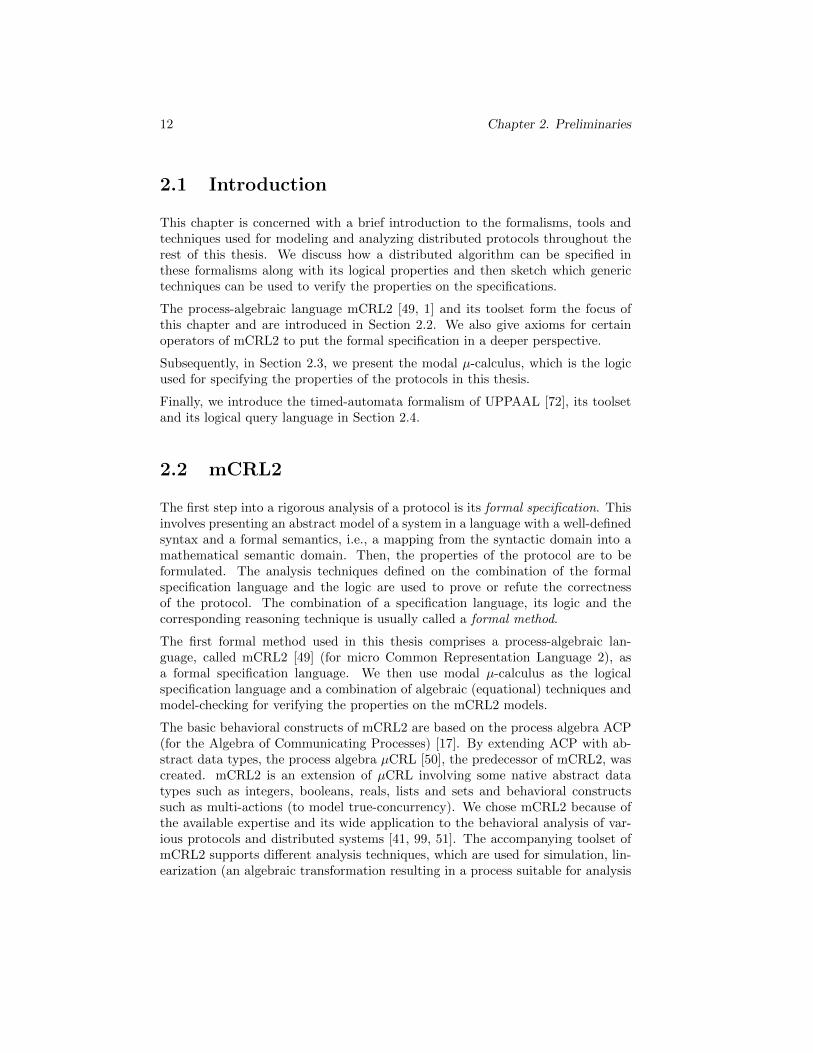
An overview of the mCRL2 toolset architecture is depicted in Figure 2.1 (thanks to[1]), where oval shapes denote the concepts used in formal analysis and rectangularshapes represent the operations over those concepts.
mCRL2Specification
µ-calculusFormula
Lineariser LinearProcess
LTSGenerator
LabeledTransistionSystem
Lineariser
PBESBES
GeneratorBES
Simulators Visualizers
Manipulators
Manipulators Manipulators
Manipulators SolverSolver
Figure 2.1 An overview of the mCRL2 toolset[1]
2.2.1 Data specification
As explained before, mCRL2 is the result of extending a process algebra witha notion of abstract data types. Hence, specification of data types is often anintegral part of an mCRL2 specification. In mCRL2, data sorts are defined usingthe keyword sort. In this way, one can define arbitrary sorts and each sort canhave a (possibly infinite) number of data elements. Constructor functions for asort are defined using the keyword cons. An example of a sort definition is givenbelow.
sort Srt;cons a, b: Srt;
14 Chapter 2. Preliminaries
In this specification, Srt is a sort name and elements of its type are denoted bya and b. Auxiliary functions to manipulate data elements are declared and theirdefining equations are given using the keywords map and eqn, respectively. Todeclare variables used in definition of an auxiliary function, the keyword var isused. As an example we define a sort Nat having two constructors zero and succ(to compute the successor) and then define an auxiliary function isEqual to checkthe equality of two natural numbers. The function isEqual returns zero if itsarguments are unequal and otherwise 1, i.e., successor of zero. (Note that Nat isa built-in type and its definition below is only for our presentation purposes. Theactual definition of Nat in mCRL2 is different, for efficiency reasons.)
sort Nat;cons zero: Nat;
succ:Nat → Nat;map isEqual:Nat×Nat→ Nat;var n,m:Nat;eqn isEqual(n,n)=succ(0);
isEqual(zero,succ(n))=zero;isEqual(succ(n),zero)=zero;isEqual(succ(n),succ(m))=eq(n,m);
mCRL2 provides built-in support for common datatypes, e.g., natural numbers(N), positive natural numbers (N+), integers (Z), real numbers (R) and booleans(B). For details we refer to [1, 50].
2.2.2 Process Specification
Atomic actions are the basic ingredients of processes. A simultaneous occurrenceof multiple actions is called a multi-action which is defined as:
α ::= τ | a | a(~d) | α|β,
where a is an atomic action, ~d is a vector of data parameters and τ is the emptymulti-action (the unit-element for |). The basic actions a and a(~d) are withoutand with data arguments, respectively. The multi-action α|β comprises the actionsfrom both the multi-actions α and β, all of which must happen at the same time.
A process specification composes actions or multi-actions using different typesof operators, most notably, alternative compositional operator (+, also calledchoice operator) and sequential compositional operators (·), e.g., p + q, p · q,where p and q are processes. To generalize the alternative compositional op-erator to parameterized processes with a parameter taken from a (possibly in-
finite) data domain, we use∑d:D
p(d) where D is some data domain. For ex-
ample, assume that a domain domain D comprises the days of a week, i.e.,
2.2 mCRL2 15
A1 x+ y = y + xA2 x+ (y + z) = (x+ y) + zA3 x+ x = xA4 (x+ y)·z = x·z + y·zA5 (x·y)·z = x·(y·z)A6 α+ δ = αA7 δ·x = δ
Cond1 true→x � y = xCond2 false→x � y = y
SUM1∑d:D x = x
SUM3∑d:DX(d) = X(e) +
∑d:DX(d)
{e is an unbounded variable in domain D}SUM4
∑d:D(X(d) + Y (d)) =
∑d:DX(d) +
∑d:D Y (d)
SUM5 (∑d:DX(d))·y =
∑d:DX(d)·y
Table 2.1 Axioms for the basic operators [53]
D = {Sat ,Sun,Mon,Tue,Wed ,Thu,Fri} then∑d:D
p(d) is equal to:
p(Sat) + p(Sun) + p(Mon) + p(Tue) + p(Wed) + p(Thu) + p(Fri).
Deadlock or inaction, denoted by δ, denotes the process that cannot perform anyaction, i.e., it has no behavior. A conditional statement is written as c → p � q,which intuitively means if c then p else q. As syntactic sugar, c→ p denotes c→p � δ. Axioms for basic operators are given in Table 2.1. Time dependent actionsare expressed as a↪t, which denotes that action a occurs at time t. Actions happenin an interleaved as well as a truly concurrent fashion when multiple processes areput in parallel using the parallel composition operator (‖). Interleaving of actionsin p ‖ q means that each action from p can happen before or after each action fromq (while preserving the internal order of actions in each of the two components).The concurrent execution of actions from p and q leads to multi-actions. Anotheroperator for putting processes in parallel is T, called left merge, which behaves likethe operator ‖ except that the first action should emanate from the first (left-hand-side) component, i.e., p in p T q; after performing its first action a left merge turnsinto a parallel composition. This operator is particularly useful in axiomatizingparallel composition (and the process of linearization, defined below). If a part ofa process is required to happen (in time) before another process, we use �, e.g.,p� q, whereas its dual is written as t� p where t is a time tag. Axioms for theparallel composition operators are given in Table 2.2.
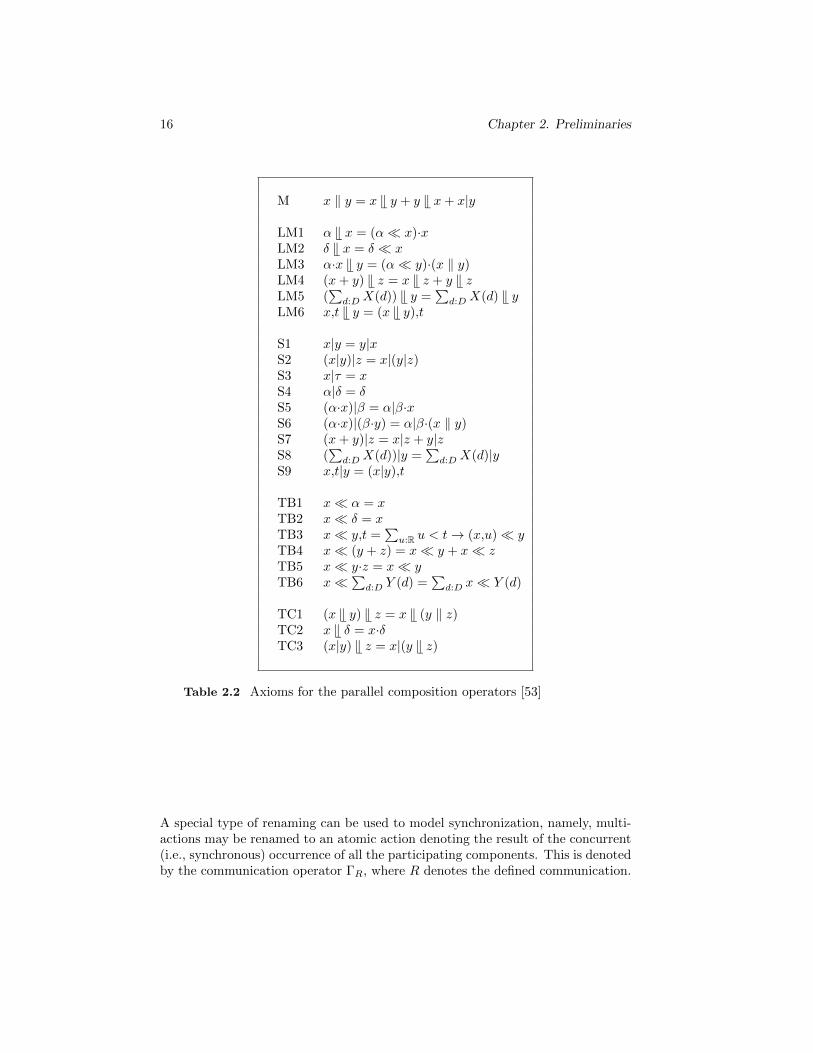
16 Chapter 2. Preliminaries
M x ‖ y = x T y + y T x+ x|y
LM1 α T x = (α� x)·xLM2 δ T x = δ � xLM3 α·x T y = (α� y)·(x ‖ y)LM4 (x+ y) T z = x T z + y T zLM5 (
∑d:DX(d)) T y =
∑d:DX(d) T y
LM6 x↪t T y = (x T y)↪t
S1 x|y = y|xS2 (x|y)|z = x|(y|z)S3 x|τ = xS4 α|δ = δS5 (α·x)|β = α|β·xS6 (α·x)|(β·y) = α|β·(x ‖ y)S7 (x+ y)|z = x|z + y|zS8 (
∑d:DX(d))|y =
∑d:DX(d)|y
S9 x↪t|y = (x|y)↪t
TB1 x� α = xTB2 x� δ = xTB3 x� y↪t =
∑u:R u < t→ (x↪u)� y
TB4 x� (y + z) = x� y + x� zTB5 x� y·z = x� yTB6 x�∑
d:D Y (d) =∑d:D x� Y (d)
TC1 (x T y) T z = x T (y ‖ z)TC2 x T δ = x·δTC3 (x|y) T z = x|(y T z)
Table 2.2 Axioms for the parallel composition operators [53]
A special type of renaming can be used to model synchronization, namely, multi-actions may be renamed to an atomic action denoting the result of the concurrent(i.e., synchronous) occurrence of all the participating components. This is denotedby the communication operator ΓR, where R denotes the defined communication.
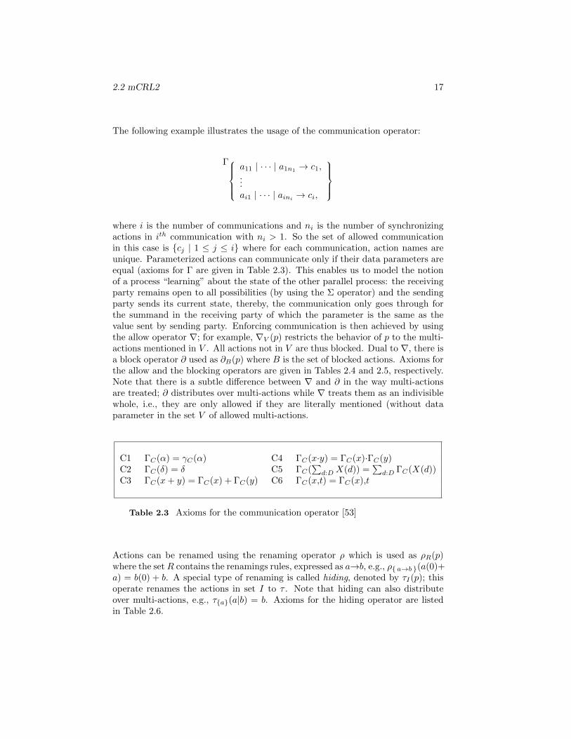
2.2 mCRL2 17
The following example illustrates the usage of the communication operator:
Γa11 | · · · | a1n1 → c1,...ai1 | · · · | aini → ci,
where i is the number of communications and ni is the number of synchronizingactions in ith communication with ni > 1. So the set of allowed communicationin this case is {cj | 1 ≤ j ≤ i} where for each communication, action names areunique. Parameterized actions can communicate only if their data parameters areequal (axioms for Γ are given in Table 2.3). This enables us to model the notionof a process “learning” about the state of the other parallel process: the receivingparty remains open to all possibilities (by using the Σ operator) and the sendingparty sends its current state, thereby, the communication only goes through forthe summand in the receiving party of which the parameter is the same as thevalue sent by sending party. Enforcing communication is then achieved by usingthe allow operator ∇; for example, ∇V (p) restricts the behavior of p to the multi-actions mentioned in V . All actions not in V are thus blocked. Dual to ∇, there isa block operator ∂ used as ∂B(p) where B is the set of blocked actions. Axioms forthe allow and the blocking operators are given in Tables 2.4 and 2.5, respectively.Note that there is a subtle difference between ∇ and ∂ in the way multi-actionsare treated; ∂ distributes over multi-actions while ∇ treats them as an indivisiblewhole, i.e., they are only allowed if they are literally mentioned (without dataparameter in the set V of allowed multi-actions.
C1 ΓC(α) = γC(α) C4 ΓC(x·y) = ΓC(x)·ΓC(y)C2 ΓC(δ) = δ C5 ΓC(
∑d:DX(d)) =
∑d:D ΓC(X(d))
C3 ΓC(x+ y) = ΓC(x) + ΓC(y) C6 ΓC(x↪t) = ΓC(x)↪t
Table 2.3 Axioms for the communication operator [53]
Actions can be renamed using the renaming operator ρ which is used as ρR(p)where the setR contains the renamings rules, expressed as a→b, e.g., ρ{ a→b }(a(0)+a) = b(0) + b. A special type of renaming is called hiding, denoted by τI(p); thisoperate renames the actions in set I to τ . Note that hiding can also distributeover multi-actions, e.g., τ{a}(a|b) = b. Axioms for the hiding operator are listedin Table 2.6.
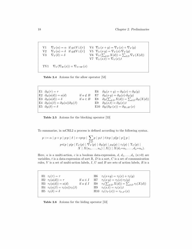
18 Chapter 2. Preliminaries
V1 ∇V (α) = α if α∈V ∪{τ} V4 ∇V (x+ y) = ∇V (x) +∇V (y)V2 ∇V (α) = δ if α 6∈V ∪{τ} V5 ∇V (x·y) = ∇V (x)·∇V (y)V3 ∇V (δ) = δ V6 ∇V (
∑d:DX(d)) =
∑d:D∇V (X(d))
V7 ∇V (x↪t) = ∇V (x)↪t
TV1 ∇V (∇W (x)) = ∇V ∩W (x)
Table 2.4 Axioms for the allow operator [53]
E1 ∂B(τ) = τ E6 ∂B(x+ y) = ∂B(x) + ∂B(y)E2 ∂B(a(d)) = a(d) if a 6∈ B E7 ∂B(x·y) = ∂B(x)·∂B(y)E3 ∂B(a(d)) = δ if a ∈ B E8 ∂B(
∑d:DX(d)) =
∑d:D ∂B(X(d))
E4 ∂B(α|β) = ∂B(α)|∂B(β) E9 ∂B(x↪t) = ∂B(x)↪tE5 ∂B(δ) = δ E10 ∂H(∂H′(x)) = ∂H∪H′(x)
Table 2.5 Axioms for the blocking operator [53]
To summarize, in mCRL2 a process is defined according to the following syntax.
p ::= α | p+ p | p·p | δ | c→p�p |∑d:D
p | p↪t | t�p | p‖p | p T p |
p�p | p|p | ΓC(p) | ∇V (p) | ∂B(p) | ρR(p) | τI(p) | ΥU (p) |X | X(u1, . . . , un) | X() | X(d1=u1, . . . , dn=un).
Here, α is a multi-action, c is a boolean data-expression, d, d1, . . . , dn (n>0) arevariables, t is a data-expression of sort R, D is a sort, C is a set of communicationrules, V is a set of multi-action labels, I, U and B are sets of action labels, R is a
H1 τI(τ) = τ H6 τI(x+y) = τI(x) + τI(y)H2 τI(a(d)) = τ if a ∈ I H7 τI(x·y) = τI(x)·τI(y)H3 τI(a(d)) = a(d) if a 6∈ I H8 τI(
∑d:DX(d)) =
∑d:D τI(X(d))
H4 τI(α|β) = τI(α)|τI(β) H9 τI(x↪t) = τI(x)↪tH5 τI(δ) = δ H10 τI(τI′(x)) = τI∪I′(x)
Table 2.6 Axioms for the hiding operator [53]
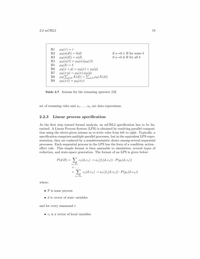
2.2 mCRL2 19
R1 ρR(τ) = τR2 ρR(a(d)) = b(d) if a→b ∈ R for some bR3 ρR(a(d)) = a(d) if a→b 6∈ R for all bR4 ρR(α|β) = ρR(α)|ρR(β)R5 ρR(δ) = δR6 ρR(x+ y) = ρR(x) + ρR(y)R7 ρR(x·y) = ρR(x)·ρR(y)R8 ρR(
∑d:DX(d)) =
∑d:D ρR(X(d))
R9 ρR(x↪t) = ρR(x)↪t
Table 2.7 Axioms for the renaming operator [53]
set of renaming rules and u1, . . . , un are data expressions.
2.2.3 Linear process specification
As the first step toward formal analysis, an mCRL2 specification has to be lin-earized. A Linear Process System (LPS) is obtained by resolving parallel composi-tion using the above-given axioms as re-write rules from left to right. Typically, aspecification comprises multiple parallel processes, but in the equivalent LPS repre-sentation, they are replaced by a nondeterministic choice among several sequentialprocesses. Each sequential process in the LPS has the form of a condition–action–effect rule. This simple format is then amenable to simulation, several types ofreduction, and state-space generation. The format of an LPS is given below:
P (d:D) =∑e1:D1
c1(d, e1)→ a1(f1(d, e1)) · P (g1(d, e1))
+ . . .
+∑en:Dn
cn(d, en)→ an(fn(d, en)) · P (gn(d, en))
where:
• P is some process
• d is vector of state variables
and for every summand i:
• ei is a vector of local variables
20 Chapter 2. Preliminaries
• ci is a condition
• ai is an action
• fi is a function used as parameter for ai
• gi computes the next state.
In mCRL2, the mcrl22lps tool is used to generate LPSs from mCRL2 specifications.The tool has several options, among others, for determining the rewriting strategyused for linearization.
An LPS can be simulated efficiently by taking the set of enabled actions and alsocalculating the parameters of the resulting process. The tools lpsxsim and lpssimare simulators, available in mCRL2.
Using lps2lts, we can generate the state space (LTS) of an LPS. Generating anLTS can be very time consuming so to make the LPS simpler the following toolscan be applied to an LPS.
• lpsconstelm (eliminates constant process parameters).
• lpsparelm (eliminates unused parameters).
• lpssumelm (eliminates superfluous summations).
Applying these reductions may even bound the state space of an infinite system.
2.2.4 LTS tools
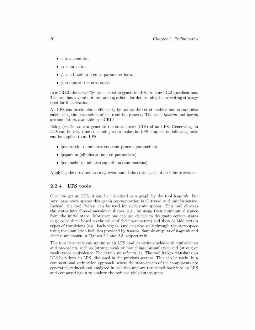
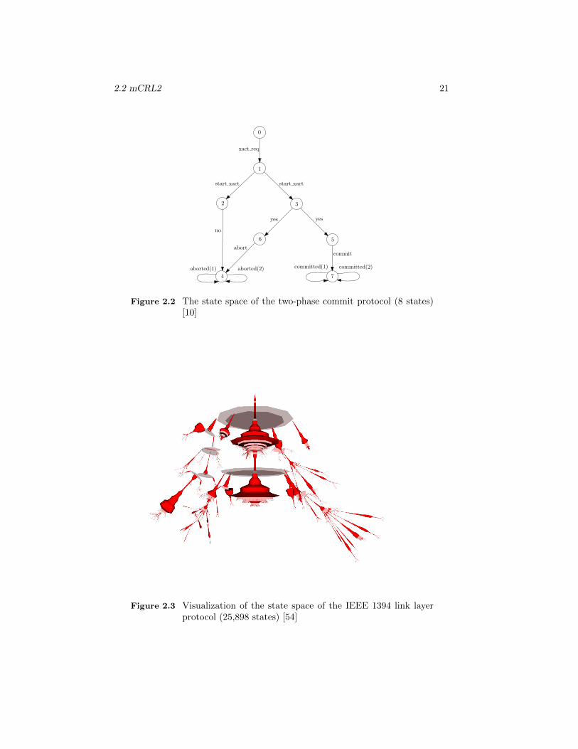
Once we get an LTS, it can be visualized as a graph by the tool ltsgraph. Forvery large state spaces this graph representation is cluttered and uninformative.Instead, the tool ltsview can be used for such state spaces. This tool clustersthe states into three-dimensional shapes, e.g., by using their minimum distancefrom the initial state. Moreover one can use ltsview to designate certain states(e.g., color them based on the value of their parameters) and show or hide certaintypes of transitions (e.g., back-edges). One can also walk through the state-spaceusing the simulation facilities provided by ltsview. Sample outputs of ltsgraph andltsview are shown in Figures 2.2 and 2.3, respectively.
The tool ltsconvert can minimize an LTS modulo various behavioral equivalencesand pre-orders, such as (strong, weak or branching) bisimulation and (strong orweak) trace equivalence. For details we refer to [1]. The tool lts2lps translates anLTS back into an LPS, discussed in the previous section. This can be useful in acompositional verification approach, where the state-spaces of the components aregenerated, reduced and analyzed in isolation and are translated back into an LPSand composed again to analyze the reduced global state-space.
2.2 mCRL2 21
xact req
start xact
no
yes yes
commit
committed(1) committed(2)aborted(2)aborted(1)
abort
0
1
2 3
4
6 5
7
start xact
Figure 2.2 The state space of the two-phase commit protocol (8 states)[10]
Figure 2.3 Visualization of the state space of the IEEE 1394 link layerprotocol (25,898 states) [54]
22 Chapter 2. Preliminaries
2.3 Modal µ-calculus
The modal µ-calculus of Kozen [63] is used to express behavioral properties oflabelled transition systems (LTSs) and is one of the most expressive variants of oftemporal logic [84]. All the properties expressible in CTL, CTL*, LTL are easilyexpressible in the modal µ-calculus [29]. A very restricted subset of the modalµ-calculus is the Hennessy-Milner logic [58], of which the BNF grammar is givenbelow:
φ ::= true | false | ¬φ | φ ∧ φ | φ ∨ φ | 〈a〉φ | [a]φ.
The diamond modality 〈a〉φ means “for some direct a successors, φ holds” and thebox modality [a]φ means “for all direct a successors, φ holds”. A useful extensionof Hennessy-Milner logic is provide by extending the modalities to action formulae,which define a set of actions. The syntax of an action formula is:
α ::= a1| · · · |an | true | false | α | α ∩ α | α ∪ α.
where
• a1| · · · |an defines the set having only the multi-action a1| · · · |an,
• false means empty set,
• true means set of all actions,
• ∩ and ∪ denote intersection and union (of sets of actions), respectively and
• α means the set of all action except α.
The resulting logic is still rather restrictive and does not allow one to specify manypractical properties such as unbounded eventualities. A straight-forward extensionis obtained by allowing for regular expression in the action formulae, as definedbelow:
R ::= ε | α | R·R| R+R | R? | R+,
where
• ε represents the empty sequence of actions,
• R1·R2 denotes the concatenation of sequences of actions in R1 and R2,
• R1+R2 denotes the union of sequences of actions in R1 and R2,
• R? means zero or more repetitions of the sequences in R and
• R+ means one or more repetitions of the sequences in R,
2.3 Modal µ-calculus 23
2.3.1 Fixed point modalities
To obtain even more expressiveness, the minimal (µ) and maximal (ν) fixed pointoperators are added the logical specification language. The fixed point operatorsµ and ν, respectively are, to some extent, analogous to the quantifiers ∃ and ∀.The grammar of the modal µ-calculus is:
φ ::= true | false | ¬φ | φ ∧ φ | φ ∨ φ | 〈a〉φ | [a]φ | µX.φ | νX.φ | X.
In this grammar, X is used to denote the class of recursive variables.
Generally, using the minimal fixed point operator liveness properties (i.e., some-thing eventually wil happen) are formulated, whereas for safety properties (i.e.,nothing bad will happen), we use the maximal fixed point operator. The fixedpoint operators are dual to each other, as given below:
¬νX.φ = µX.¬φ ¬µX.φ = νX.¬φ
2.3.2 Modal formulae with data and quantifiers
Due to the genuine presence of data elements in mCRL2 specification, there is aneed to extend the logical language of modal µ-calculus with data. The additionof data to the modal µ-calculus results in a very expressive logic, in which dataexpressions cannot only be used to refer to the occurrence of parameterized actionsbut also can be used to parameterize the recursive variables, e.g., allowing forcounting the occurrence of a certain action. The syntax of this expressive logic isgiven below.
α ::= τ | a(t1, . . . , tn) | α|α.af ::= t | true | false | α | af | af ∩ af | af ∪ af | ∀d:D.af | ∃d:D.af | af ↪u.R ::= ε | af | R·R | R+R | R? | R+.φ ::= true | false | t | ¬φ | φ ∧ φ | φ ∨ φ | φ→ φ | ∀d:D.φ | ∃d:D.φ | 〈R〉φ |
[R]φ | µX(d1:D1:=t1, . . . , dn:Dn:=tn).φ |νX(d1:D1:=t1, . . . , dn:Dn:=tn).φ | X(t1, . . . , tn).
Existential (∃) and universal quantifier (∀) are also included in this language whichallow for concise specification of parameterized logical properties. For, example,consider the consensus protocol where a process p is allowed to decide only onceon any value from a give domain V . This formula is expressed as:
∀p∈π,∀v ,v ′∈V [true∗ · decide(p, v) · true∗ · decide(p, v′)]false,
where π is the set of participants in the protocol and decide(p, v) is the actionwhich denotes that process p has decided on value v. This property is discussedin more detail in Chapter 4, Section 4.4.1.
24 Chapter 2. Preliminaries
2.3.3 Model checking using PBESs
Model checking is a technique used to exhaust the state-space of a system in orderto determine whether a modeled system satisfies the desired/claimed properties.Boolean Equation Systems (BESs) have been proposed as a means to to verifymodal µ-calculus formulae on transition systems [75]. In mCRL2, parameterizedboolean equation systems (PBESs) are used as an intermediate representation formodel checking logical properties with data on mCRL2 specifications; PBESs areessentially an extension to BESs with data. In the mCRL2 toolset, the model andits property are encoded into a PBES and solving that PBES leads to the solutionof the model checking problem, i.e., if the initial variable of the PBES is solved tobe true then the property is satisfied and otherwise a counterexample is generatedwitnessing why the property is violated. A PBES contains a sequence of equationsof the following form:
σXi(d1 : D1, . . . , dn : Dn) = ϕi,
where i ∈ N, σ denotes either the least fixed point (µ) or the greatest fixed point(ν) operator, di is data of type Di, Xi is a predicate variable and ϕi is a predicateformula. The syntax of a predicate formula is given below:
ϕ ::= b | X(~e) | ϕ⊕ ϕ | Qd:D.ϕ,
where b is a data term of sort boolean, ⊕ ∈ {∧,∨}, Q ∈ {∀,∃}, X is predicatevariable, d is a data variable of some sort D and e is also a data term.
Although solving a PBES in general is undecidable, practically it is observed thatby adopting pragmatic approaches like simplifying and/or rewriting a PBES, wecan solve a PBES in most cases, cf. the results discussed in Chapter 5 and [55].To apply this technique we need an LPS and a µ-calculus formula (expressinga desired property). The tool lps2pbes generates a PBES which is solved usinganother tool pbes2bool to get either true if the formula holds or otherwise false.
2.4 UPPAAL
2.4.1 The specification language
Another formal method that is used in this thesis is based on the theory of timedautomata, which is incarnated in the UPPAAL toolset [71]. UPPAAL is a toolboxused for modeling and verification of real-time distributed systems. The specifi-cation language of UPPAAL is an extension of the well-known timed automata ofAlur and Dill [2, 102]. One of the main extensions concerns allowing for communi-cation of timed automata, leading to a network of timed automata. The behavioral
2.4 UPPAAL 25
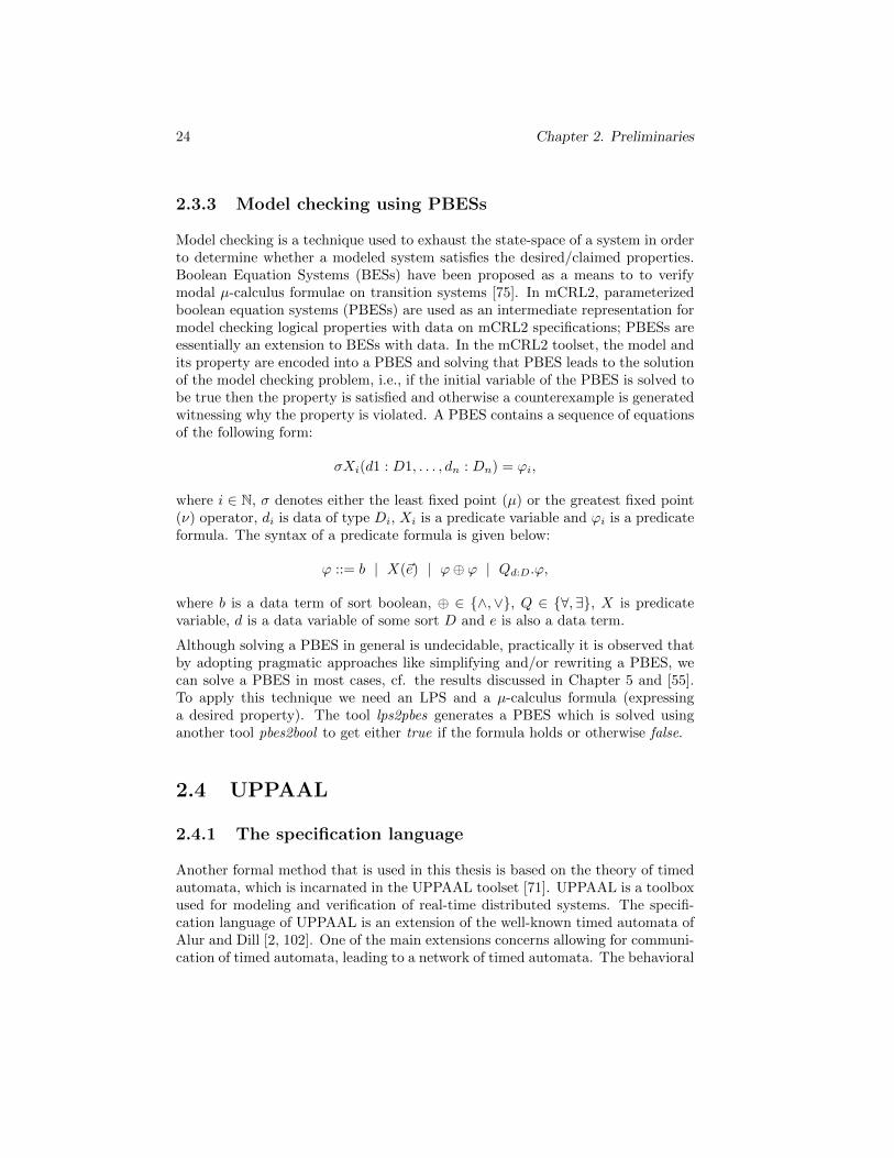
specification of a process type, called template, is described as a timed automa-ton. Processes can be instantiated from templates and composed using parallelcomposition to form the description of the system. Time-based transitions are putinto effect by means of real-valued clocks as introduced in the standard timed au-tomata. Time is supposed to be continuous and all the clocks declared in a systemprogress simultaneously with the same rate. Every automaton has an initial loca-tion, denoted by a double circle. Each transition from one location to another canbe guarded by a boolean expression comprising local and global variables as wellas certain clock expressions (e.g., comparing a clock against a constant). Duringa transition, a process can synchronize with another process (handshaking) or canbroadcast a message for multiple recipients using channels. For example, automatafor train and gate in the train-gate example (thanks to [18]) are shown in Figures2.4(a) and 2.4(b), respectively.
Safe
Stop
Crossx<=5
Apprx<=20
Startx<= 15
x>=10x=0
x<=10stop[id]?
x>=3leave[id]!
appr[id]!x=0
x>=7x=0
go[id]?x=0
(a) The train automaton
Occ
Free
e : id_tappr[e]?enqueue(e)
e : id_te == front()leave[e]?dequeue()
stop[tail()]!
len > 0go[front()]!
e : id_tlen == 0appr[e]?enqueue(e)
(b) The gate automaton
Figure 2.4 A train-gate example in UPPAAL
A location can be marked as urgent or committed, denoted, respectively, by en-circled “U” or “C”. The former means that time is not allowed to progress whileresiding in that location. Committed, in addition to being urgent, has the prop-erty that the transition at the system level should be a transition from one of thecurrent committed states. Urgent locations are helpful to enforce progress andcommitted locations reduce the state space due to the reduced possibilities forinterleaving with other transitions from other processes, i.e., non-committed ones.Furthermore, locations can be given invariants (in terms of boolean expressions,possibly involving clocks), which should hold as long as the system resides in thestate.
UPPAAL provides the following four data types:
26 Chapter 2. Preliminaries
int: For integers, ranging from -32768 to 32767.
bool: For booleans, true or false.
clock: For time, clocks evaluate to a real number.
chan: For channels, used for hand-shaking synchronization or broadcasting.
UPPAAL also supports scalars which are integer-like elements used for symme-try reduction, a technique used in state space reduction [57]. This technique ishelpful when a system model contains multiple symmetrically behaving processes.Allowed operators with scalars of the same type are testing (in)equality (= or 6=)and assignment (:=). Symmetry reduction has been successfully applied to theverification of systems and protocols, e.g., in [42, 89, 46] and Chapter 6 of thisthesis.
2.4.2 The query language
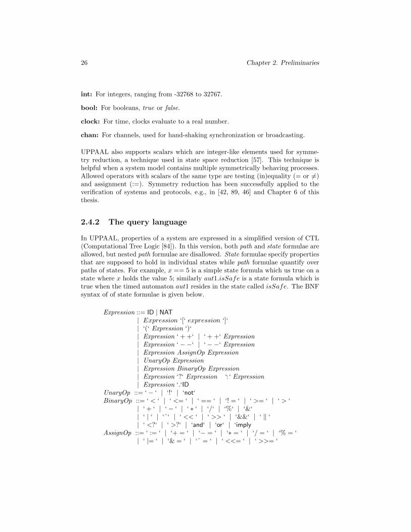
In UPPAAL, properties of a system are expressed in a simplified version of CTL(Computational Tree Logic [84]). In this version, both path and state formulae areallowed, but nested path formulae are disallowed. State formulae specify propertiesthat are supposed to hold in individual states while path formulae quantify overpaths of states. For example, x == 5 is a simple state formula which us true on astate where x holds the value 5; similarly aut1.isSafe is a state formula which istrue when the timed automaton aut1 resides in the state called isSafe. The BNFsyntax of of state formulae is given below.
Expression ::= ID | NAT| Expression ‘[‘ expression ‘]‘| ‘(‘ Expression ‘)‘| Expression ‘ + +‘ | ‘ + +‘ Expression| Expression ‘−−‘ | ‘−−‘ Expression| Expression AssignOp Expression| UnaryOp Expression| Expression BinaryOp Expression| Expression ‘?‘ Expression ‘:‘ Expression| Expression ‘.‘ID
UnaryOp ::= ‘− ‘ | ‘!‘ | ‘not‘BinaryOp ::= ‘ < ‘ | ‘ <= ‘ | ‘ == ‘ | ‘! = ‘ | ‘ >= ‘ | ‘ > ‘
| ‘ + ‘ | ‘− ‘ | ‘ ∗ ‘ | ‘/‘ | ‘%‘ | ‘&‘| ‘ | ‘ | ‘ˆ‘ | ‘ << ‘ | ‘ >> ‘ | ‘&&‘ | ‘ ‖ ‘| ‘ <?‘ | ‘ >?‘ | ‘and‘ | ‘or‘ | ‘imply
AssignOp ::= ‘ := ‘ | ‘+ = ‘ | ‘− = ‘ | ‘∗ = ‘ | ‘/ = ‘ | ‘% = ‘| ‘ |= ‘ | ‘& = ‘ | ‘ˆ = ‘ | ‘ <<= ‘ | ‘ >>= ‘
2.4 UPPAAL 27
Most of the syntax is self-explanatory and has the same intuition as in program-ming languages. ID stands for identifiers, including variable and state names.The operators not, and, or, imply are logical operators for negation, and, or andimplication, respectively. The operators ‘ <?‘ and ‘ >?‘, respectively, determinethe minimum and the maximum of two integers. To check the occurrence of adeadlock state (a state from which there is no outgoing transition), the keyworddeadlock can be used.
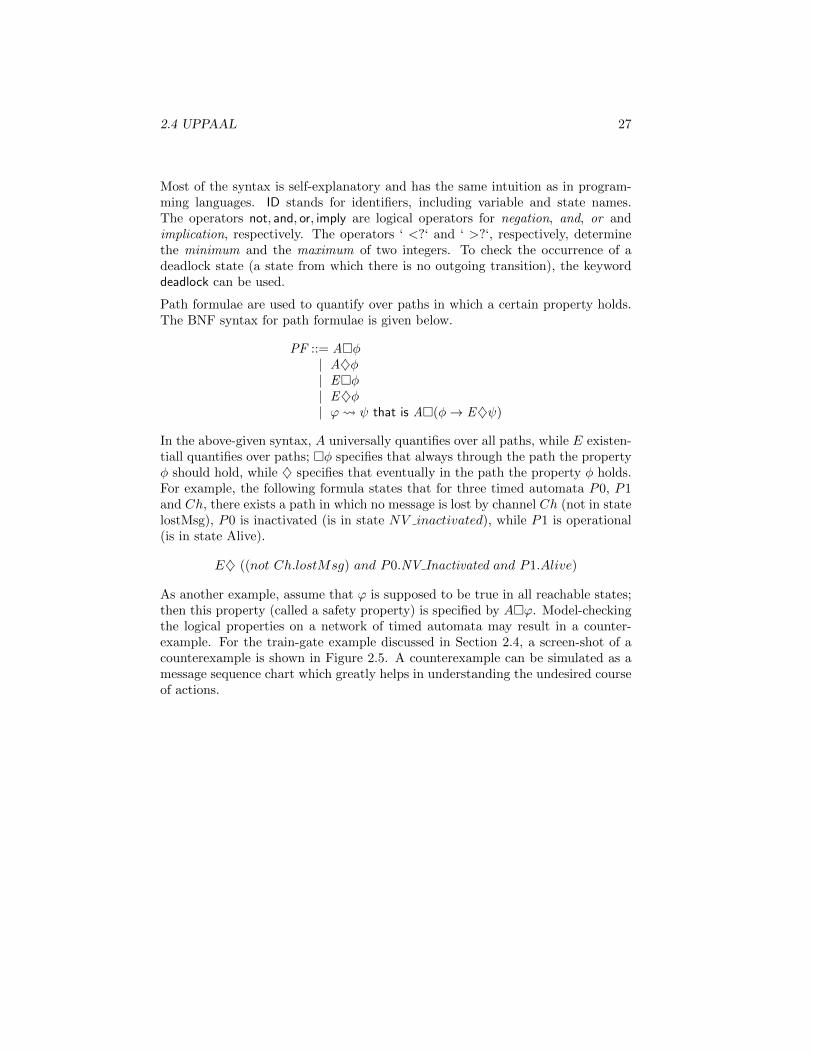
Path formulae are used to quantify over paths in which a certain property holds.The BNF syntax for path formulae is given below.
PF ::= A�φ| A♦φ| E�φ| E♦φ| ϕ ψ that is A�(φ→ E♦ψ)
In the above-given syntax, A universally quantifies over all paths, while E existen-tiall quantifies over paths; �φ specifies that always through the path the propertyφ should hold, while ♦ specifies that eventually in the path the property φ holds.For example, the following formula states that for three timed automata P0, P1and Ch, there exists a path in which no message is lost by channel Ch (not in statelostMsg), P0 is inactivated (is in state NV inactivated), while P1 is operational(is in state Alive).
E♦ ((not Ch.lostMsg) and P0.NV Inactivated and P1.Alive)
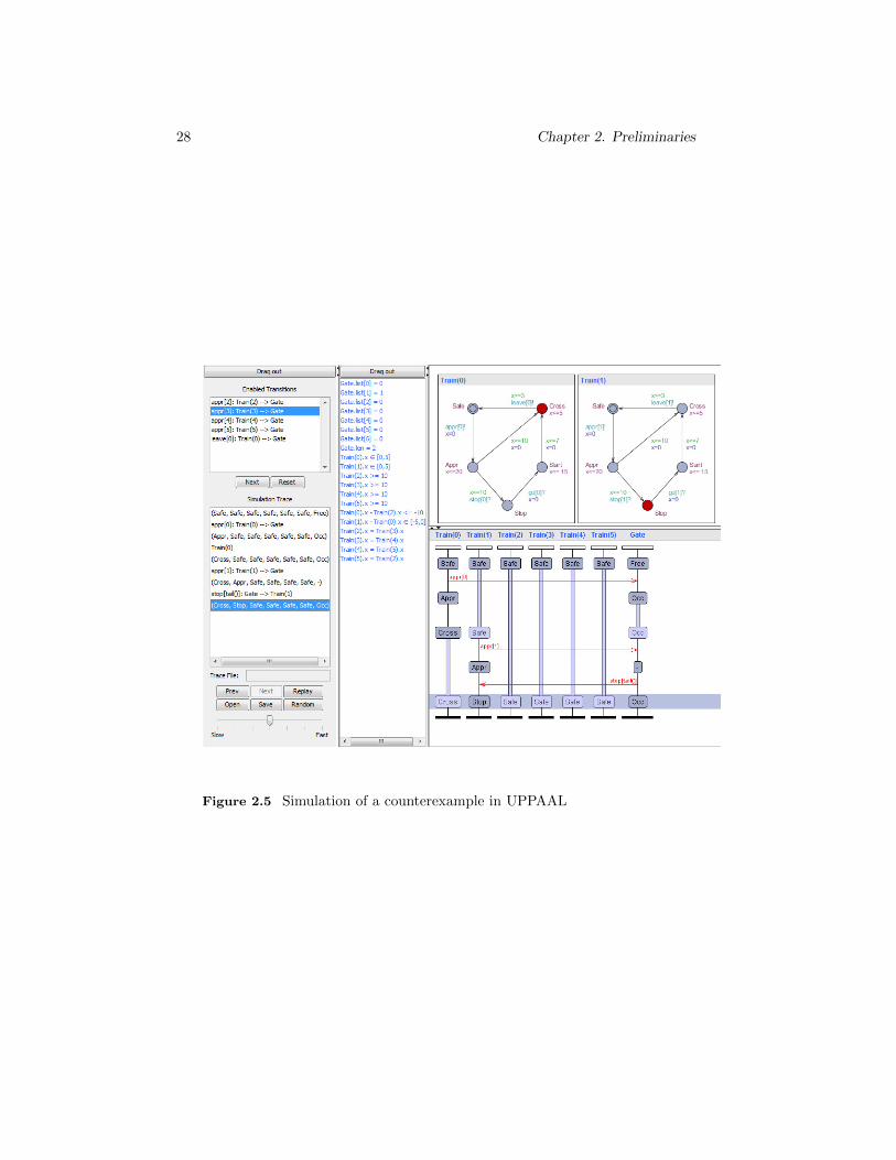
As another example, assume that ϕ is supposed to be true in all reachable states;then this property (called a safety property) is specified by A�ϕ. Model-checkingthe logical properties on a network of timed automata may result in a counter-example. For the train-gate example discussed in Section 2.4, a screen-shot of acounterexample is shown in Figure 2.5. A counterexample can be simulated as amessage sequence chart which greatly helps in understanding the undesired courseof actions.
28 Chapter 2. Preliminaries
Figure 2.5 Simulation of a counterexample in UPPAAL
Chapter 3
Formal Specification andAnalysis of AcceleratedHeartbeat Protocols
In: Proceedings of the Summer Computer Simulation Conference 2010 (SCSC 2010), TheSociety for Modeling & Simulation International, Book 1 of 3, ISBN 978-1-61738-702-9.
30 Chapter 3. Accelerated Heartbeat Protocols
3.1 Introduction
In this chapter, we present a formal analysis of all different variations of acceler-ated heartbeat protocols presented in [47]. We formalize the specification of theprotocols in a process algebraic formalism. Then, we formulate some natural func-tional requirements on the above-mentioned protocols in the modal µ-calculus.Using model-checking techniques, we verify these requirements on each and everyversion. We report counterexamples witnessing that the formulated requirementsare not satisfied. We propose fixes for different versions of the protocol and modelcheck the fixed versions; the model checking results indicate that the fixed versionsindeed satisfy the requirements.
Heartbeat protocols are used as the underlying synchronization mechanism formany other distributed protocols [48, 61, 95, 100, 101]. The basic idea behind aheartbeat protocol is that once a participating process or a communication chan-nel crashes, other processes become aware of this fact and become inactive withina certain interval. To this end, processes periodically exchange simple messages,called heartbeats, to inform each other about their liveness. If an expected heart-beat is not received after a specific time, it is assumed that either the respectiveprocess has failed or the communication medium is down. After a number of pe-riods without any response, the expecting processes eventually become inactive,thus guaranteeing timely inactivation of all participants after a process or channelcrash. In other words, heartbeat protocols can be considered as simplified versionsand/or building blocks of more sophisticated failure detector protocols.
In [47], several variations of heartbeat protocols are presented. These protocols aimat achieving the above-mentioned goal while reducing the overhead, i.e., the rateof heartbeat transmissions. This is why the protocols in [47] are called acceleratedheartbeat protocols. Moreover, they try to minimize the detection delay (theinterval between the crash and the deactivation of all processes) and maximizereliability (minimizing the probability of inactivation due to lost heartbeats).
We formally model and analyze all different versions of heartbeat protocols pre-sented in [47]. To this end, we give a formal specification of these protocols in twoformalisms: the process algebra mCRL2 [50] and the timed-automata language ofUPPAAL [72]. Note that both process-algebraic and automata-theoretic modelsare complete models of the protocols and can be independently used to present thesame results. Then, we specify basic properties about the safety and liveness of theprotocols, namely that upon a crash, all processes will eventually be deactivatedwithin a certain period of time (to be specified precisely by the protocol specifi-cation) and if no process crashes and no message is lost or delayed (beyond itsallowed limit), then no process will decide to deactivate (i.e., suspect any crash).We verify these, rather basic, requirements on the protocols given in [47]. For theprocess algebraic specification, we specify the requirements using a combination ofmonitor processes and modal µ-calculus formulae and use the Caesar/Aldebaran
3.2 Accelerated heartbeat protocols 31
tool-set [45] to model-check the specified properties on the formal specification ofthe protocols. For the automata-theoretic specifications, we use a combination ofmonitor timed-automata and reachability properties and use UPPAAL to model-check them. To our surprise, for each of the protocols we found situations whereone or both of the above properties are not satisfied. In [78], slightly modifiedversions of some of the protocols in [47] are presented. We have also analyzed themodified versions and briefly discuss the results in the remainder of this chapter.To our knowledge, the heartbeat protocols studied in this chapter have not beenformally analyzed before in the literature. An extended version of this chapter ispresented in [13].
Structure of the chapter. Heartbeat protocols are presented informally inSection 3.2. In Sections 3.3 and 3.4, respectively, we give an overview of theprocess-algebraic and the automata-theoretic specification of the protocol. Section3.5 is devoted to the specification of requirements and their analysis. In Section3.6, the discovered counterexamples are discussed and some fixes for the protocolsare proposed. The fixed versions of the protocol are then model-checked and shownto be correct. The Chapter is concluded in Section 3.7.
3.2 Accelerated heartbeat protocols
In this section, we briefly present the following four different types of acceleratedheartbeat protocols introduced in [47].
1. The binary heartbeat protocol.
2. The static heartbeat protocol.
3. The expanding heartbeat protocol.
4. The dynamic heartbeat protocol.
All the protocols, to be presented in the remainder of this section, have the fol-lowing basic assumptions in common.
1. Every process is active in the beginning.
2. Any active process can become inactive anytime (due to a crash) but cannotbecome active again (recover) afterwards. (We call the crash of a processits voluntary inactivation, as opposed to non-voluntary inactivation, whichis caused by the protocol.)
32 Chapter 3. Accelerated Heartbeat Protocols
3. Every sent message will be received provided that the communication mediumis up. In particular, messages sent to crashed processes will be received butwill be given no reply. If a message is to be delivered (the channel is up), itis delivered within a certain period of time; the maximum round-trip delayof channels is bound by the constant tmin.
3.2.1 The binary heartbeat protocol
In this protocol, only two processes participate in exchanging their heartbeats ina round-based fashion. Let p[0] and p[1] be the processes and tmax and tmin bethe maximum and minimum waiting time, respectively, for each round. Let t bethe waiting time of p[0] for each round such that tmin ≤ t ≤ tmax. (Note thattmin is the same constant as the upper bound on the round-trip channel delays.)The process p[0] iteratively follows the steps given below to run the protocol:
1. It waits for a period of length t, where t is initially set to tmax.
2. It sends a heartbeat message to p[1].
3. For the next round, the value for t is tmax if p[0] has received the heartbeatfrom p[1] in the current round, or otherwise t becomes t/2. However, if thenew value of t is less than tmin, p[0] itself becomes inactive (non-voluntarily).
To respond to p[0], p[1] performs the following three steps.
1. Receives a heartbeat from p[0].
2. Sends its heartbeat.
3. If it does not receive a heartbeat from p[0] for a period of length 3tmax−tmin,it becomes inactive (non-voluntarily).
In [78], a slightly modified version of the binary (and static) heartbeat protocolsare presented, in which p[0] does not wait initially but starts off by sending itsheartbeat to p[1]. In the remainder of this chapter, we refer to this version as therevised binary heartbeat protocol.
Also, a modified version of binary heartbeat protocol, called two-phase heartbeatprotocol, is presented in [47]. In the two-phase heartbeat protocol the value of t isreduced immediately to tmin if p[0] does not receive a heartbeat from p[1] in theprevious round. Otherwise, the specification of the two-phase heartbeat protocolis identical to its binary counterpart.
3.2 Accelerated heartbeat protocols 33
3.2.2 The static heartbeat protocol
The static heartbeat protocol extends the binary heartbeat protocol by allowingfor a fixed number of participating processes. In this protocol, p[0] broadcasts itsheartbeat to n processes, where the value of n is fixed and a priori known to p[0].Process p[0] exchanges heartbeat messages periodically by executing the binaryheartbeat protocol with every p[i], where 1 ≤ i ≤ n. (Note that all heartbeatexchanges are with p[0] and other processes do not exchange their heartbeatsamong themselves.) All of the processes in the network commonly use the valuesof tmax and tmin (introduced in Section 3.2.1). Process p[0] maintains a listof type Boolean to record the response of every process with respect to its sentheartbeats. It assigns the value true, if it receives a heartbeat within t time units,or otherwise false to the respective process. Process p[0] also maintains a list oftime periods tm (initialized with tmax as the value of all cells), indicating thewaiting time for each process. This list is changed after each round accordingto the received heartbeat from respective process(es), using the same proceduredescribed for t in Section 3.2.1, i.e., after each round, if p[0] receives a heartbeatfrom p[i] within t time units, then the value of tm[i] is set to tmax, otherwise, it isset to tm[i]/2. In each round, the waiting time t of p[0] is defined by min(tm[1..n]).
3.2.3 The expanding heartbeat protocol
The expanding heartbeat protocol extends the static heartbeat protocol in that theparticipating processes may join the protocol gradually in the course of protocolexecution. At the start of this protocol, p[0] is the only process and later anynumber of other processes can join by sending their heartbeats. The new processrecognizes that it has joined the protocol when it receives the heartbeat from p[0];otherwise, it continues sending its heartbeat every tmin time units until the limit3tmax − tmin is reached, upon which it decides that p[0] or the communicationchannel has crashed and goes to the (non-voluntarily) inactivated state. Processp[0] maintains the list jnd of joined processes and executes the static heartbeatprotocol with them. The response time and waiting time of each process andeach round, respectively, are computed exactly as in the static heartbeat protocol,discussed in Section 3.2.2.
3.2.4 The dynamic heartbeat protocol
This version is the most flexible one as compared to the other protocols introducedin [47]. Each process can join and then leave (permanently) at will. To encode joinand leave messages in this protocol, heartbeats are parameterized with a booleanparameter. For joining or remaining in protocol, heartbeats carry true and forleaving, they carry false as the data parameter. If a process p[i] decides to join
34 Chapter 3. Accelerated Heartbeat Protocols
the protocol, it keeps on sending its heartbeat with parameter true every tminunits of time. Receiving a heartbeat with parameter true from p[0] indicates thatp[i] has actually joined the protocol. Again if p[i] does not receive a heartbeatwith parameter true within a period of 3tmax − tmin, p[i] will assume a crash inthe nodes or channels and will inactivate itself non-voluntarily. When joined theprotocol, the specification of p[i] is identical to the expanding version, except forthe fact that it can leave the protocol by sending heartbeats with parameter false.Again, p[0] acknowledges this by sending a heartbeat with the same parameter. Itis important to differentiate between leaving the protocol and crashing (voluntarilybecoming inactive). The former will not affect the other participants at all whilethe latter will cause the inactivation of every process in the network.
3.3 Formal specification in mCRL2
3.3.1 Introduction
In this section, first we present a general overview of our formal specification inthe process algebraic formalism mCRL2 and then the notational aspects of theformalism used in our specification of the accelerated heartbeat protocols. Ourformal specification in mCRL2 comprises the following aspects.
Data types. The first part of our formal specification is dedicated to formalizingthe data types used in the specification of the protocol. This part involves nonovelty, as data types such as booleans, integers and lists are already built inthe mCRL2 syntax and we only need to compose them in order to obtain morecomplex data structures. Also, we defined straightforward operations on thesedata types to check and update data values in different data structures.
Main processes. The participants of the protocols are modeled as a choiceamong a number of sequential processes, each of which are triggered by a cer-tain event. For example, the specification of process p[0] in the binary heartbeatprotocol comprises the following choices:
1. crashing,
2. receiving a heartbeat from p[1],
3. receiving a time-out (t time units after sending the heartbeat), checkingwhether a heartbeat is received from p[1], and either becoming inactivatednon-voluntarily or adjusting the next waiting time accordingly,
4. passing one time unit.

3.3 Formal specification in mCRL2 35
The structure of p[1] is very similar to that of p[0]; it only replies to the heartbeatreceived from p[0] right away and has a time-out on 3tmax − tmin resulting inimmediate non-voluntary inactivation.
The structure of the main processes in the other three versions are quite simi-lar, except that more choices are added to the specification (e.g., for joining andleaving the protocol) and more details are added to each sequential process (e.g.,calculating the minimum of the list of waiting times).
Channels. Channels are simple processes, which receive a message from oneside and non-deterministically decide to lose it or deliver it to the other side. Weexplain below how the upper-bound on the round-trip delay of channels is enforced.
Timing. Timing constraints play a crucial role in the heartbeat protocols; theyare both present in the protocol specification as well as in the correctness require-ments. In the current version of the mCRL2 toolset, there is limited support forthe analysis of timed specification. Hence, we have set up auxiliary processes whichact as clocks and watchdogs for the actual processes participating in the protocols.There is an underlying clock synchronization mechanism, which enforces differentclocks to proceed at the same speed. This is achieved by a multi-party synchro-nization among clocks (using the so called multi-actions in mCRL2). Moreover,timeouts are implemented as watchdog processes that start ticking when they re-ceive a message corresponding to their triggering event (e.g., sending a heartbeatby p[0] for the watchdog taking care of timeout at t in p[0]) and sending an un-delayable message to the process to be triggered after a certain amount of time(e.g., issuing a timeout message for p[0] after passing t time units from sendingits heartbeat). A similar watchdog mechanism is used to enforce a maximumround-trip delay on channels; the heartbeats are timestamped with their delaywhen delivered from p[0] to each p[i] and the corresponding watchdog will resumecounting down from the point it has left when the replying heartbeat is set on thechannel in the reverse direction. For broadcast messages delays are controlled bya separate watchdog for each process.
We next give an overview of the formal specification of main processes in ourformalization of the binary heartbeat protocol and point out the changes that aremade in order to obtain the other versions of the protocol.
3.3.2 The binary heartbeat protocol in mCRL2
Process p[0]
We define process p[0] by means of following five parameters. Here “Bool” and“Nat” are sorts (types) [50] for boolean and natural numbers respectively.
36 Chapter 3. Accelerated Heartbeat Protocols
• active : Bool. A flag that shows the state of process, i.e., true if activeotherwise false. The initial value for this parameter is true.
• rcvd : Bool. A flag that denotes the receiving a reply from p[1], i.e., true ifreceived, or otherwise false. The initial value for this parameter is true.
• t : Nat. Length of the time period to exchange the beat messages, of whichthe initial value is tmax.
• tmin : Nat. Lower bound for waiting time of each round.
• tmax : Nat. Upper bound for waiting time of each round.
Specification of p[0]: 1
1: P0(t : Nat, active, rcvd : Bool, tmin, tmax : Pos) =2: tick p0.P0(t, active, true, tmin, tmax)3: +4: active→ inactivate v p0.P0(t, false, rcvd, tmin, tmax)5: +6: from p1(hb1).(active→ P0(tmax, active, true, tmin, tmax)7: �8: P0(tmax, active, false, tmin, tmax))9: +
10: active→ (timeout at P0.11: (rcvd→ for p1(hb0).send ticking time(tmax).12: P0(tmax, active, false, tmin, tmax)13: �14: t div 2 ≥ tmin→ for p1(hb0).15: send ticking time(t div 2).16: P0(t div 2, active, false, tmin, tmax)17: �18: inactivate nv p0.P0(tmax, false, rcvd, tmin, tmax)19: )20: );
Process p[0] comprises four summands separated by nondeterministic choice (de-noted by +). In line 2 of the above specification for p[0], tick p0 denotes theclock tick, which allows for time to pass and in line 4, an active process may non-deterministically voluntarily decide to become inactivated. (Notation c→ p0 � p1
stands for “if c then p0 else p1; when the else part is not mentioned, it is assumedto be deadlock. In case of mCRL2 processes without timed actions, deadlock isthe unit element for non-deterministic choice.) Line 6 shows that the process canreceive the heartbeat of p[1] without any precondition using an action from p1.
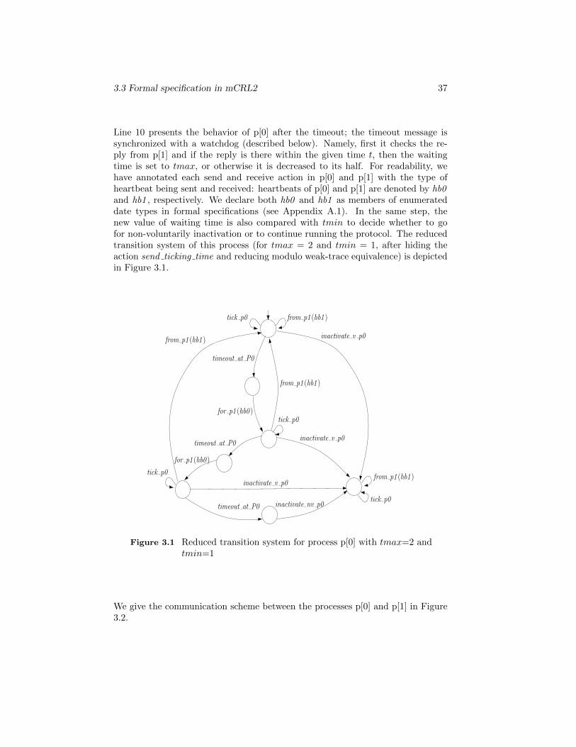
3.3 Formal specification in mCRL2 37
Line 10 presents the behavior of p[0] after the timeout; the timeout message issynchronized with a watchdog (described below). Namely, first it checks the re-ply from p[1] and if the reply is there within the given time t, then the waitingtime is set to tmax, or otherwise it is decreased to its half. For readability, wehave annotated each send and receive action in p[0] and p[1] with the type ofheartbeat being sent and received: heartbeats of p[0] and p[1] are denoted by hb0and hb1 , respectively. We declare both hb0 and hb1 as members of enumerateddate types in formal specifications (see Appendix A.1). In the same step, thenew value of waiting time is also compared with tmin to decide whether to gofor non-voluntarily inactivation or to continue running the protocol. The reducedtransition system of this process (for tmax = 2 and tmin = 1, after hiding theaction send ticking time and reducing modulo weak-trace equivalence) is depictedin Figure 3.1.
tick p0 from p1 (hb1 )
from p1 (hb1 )
tick p0
inactivate v p0
timeout at P0
for p1 (hb0 )
from p1 (hb1 )
timeout at P0
for p1 (hb0 )
from p1 (hb1 )
inactivate v p0
inactivate nv p0timeout at P0
inactivate v p0
tick p0
tick p0
Figure 3.1 Reduced transition system for process p[0] with tmax=2 andtmin=1
We give the communication scheme between the processes p[0] and p[1] in Figure3.2.
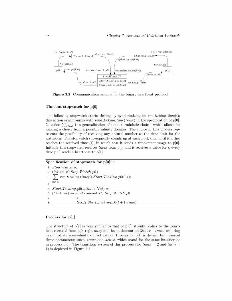
38 Chapter 3. Accelerated Heartbeat Protocols
p[0] p[1]
Stop Watch Ch
Start T icking p0 to p1
Start T icking p1 to p0
Channel p0 to p1 Channel p1 to p0
for p1(hb0)
from p1(hb1)
rcv from p0(hb0)start sw ch(hb0)
rcv from p1(hb1)
update sw ch(hb1)
rcv update sw ch(hb1)rcv start sw ch(hb0)
send to p1(hb0)
from p0(hb0)
for p0(hb1)
send to p0(hb1)
Figure 3.2 Communication scheme for the binary heartbeat protocol
Timeout stopwatch for p[0]
The following stopwatch starts ticking by synchronizing on rcv ticking time(i);this action synchronizes with send ticking time(tmax ) in the specification of p[0].Notation
∑i:Nat is a generalization of nondeterministic choice, which allows for
making a choice from a possibly infinite domain. The choice in this process rep-resents the possibility of receiving any natural number as the time limit for thewatchdog. The stopwatch subsequently counts up at each clock tick, until it eitherreaches the received time (i), in which case it sends a time-out message to p[0].Initially this stopwatch receives tmax from p[0] and it receives a value for i, everytime p[0] sends a heartbeat to p[1].
Specification of stopwatch for p[0]: 2
1: Stop Watch p0 =2: tick sw p0.Stop Watch p0+
3:∑i:Nat
rcv ticking time(i).Start T icking p0(0, i);
4:
5: Start T icking p0(t, time : Nat) =6: (t ≈ time)→ send timeout P0.Stop Watch p07: �8: tick 2.Start T icking p0(t+ 1, time);
Process for p[1]
The structure of p[1] is very similar to that of p[0]; it only replies to the heart-beat received from p[0] right away and has a timeout on 3tmax− tmin, resultingin immediate non-voluntary inactivation. Process for p[1] is defined by means ofthree parameters; tmin, tmax and active, which stand for the same intuition asin process p[0]. The transition system of this process (for tmax = 2 and tmin =1) is depicted in Figure 3.3.
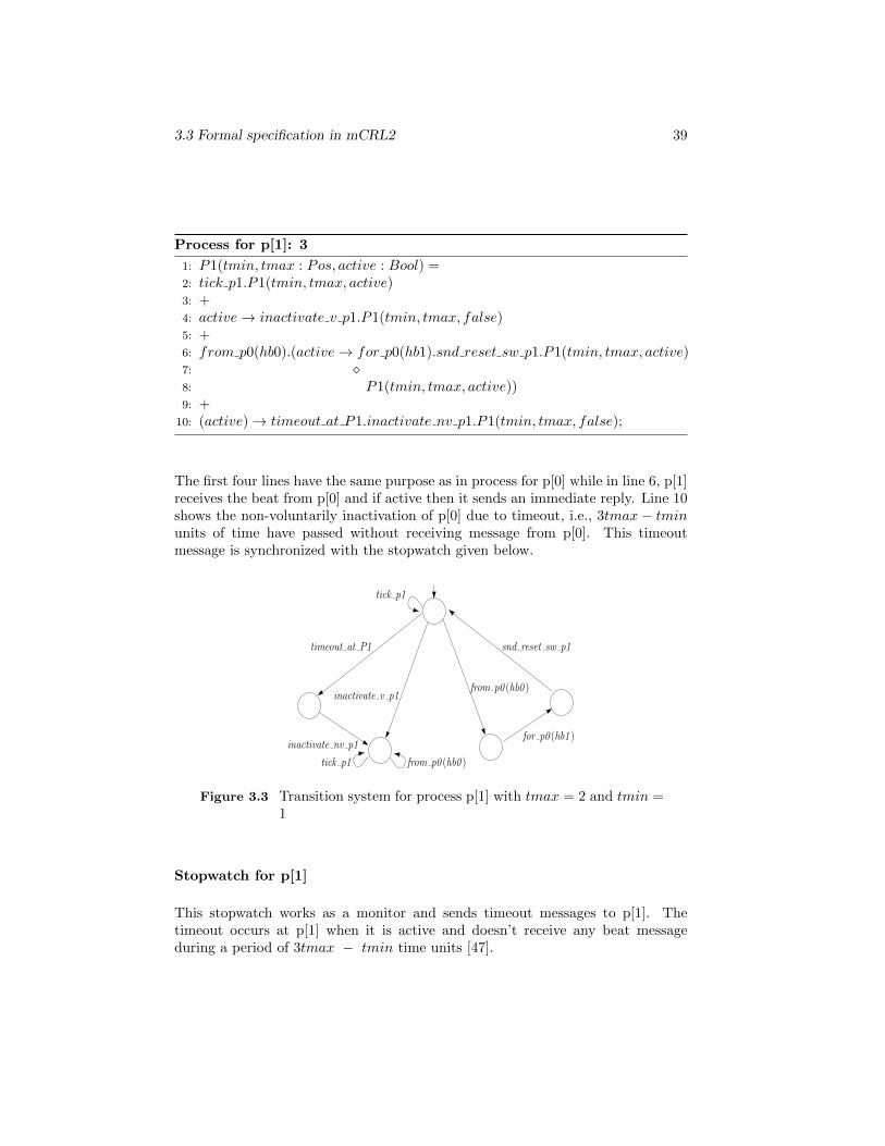
3.3 Formal specification in mCRL2 39
Process for p[1]: 3
1: P1(tmin, tmax : Pos, active : Bool) =2: tick p1.P1(tmin, tmax, active)3: +4: active→ inactivate v p1.P1(tmin, tmax, false)5: +6: from p0(hb0).(active→ for p0(hb1).snd reset sw p1.P1(tmin, tmax, active)7: �8: P1(tmin, tmax, active))9: +
10: (active)→ timeout at P1.inactivate nv p1.P1(tmin, tmax, false);
The first four lines have the same purpose as in process for p[0] while in line 6, p[1]receives the beat from p[0] and if active then it sends an immediate reply. Line 10shows the non-voluntarily inactivation of p[0] due to timeout, i.e., 3tmax− tminunits of time have passed without receiving message from p[0]. This timeoutmessage is synchronized with the stopwatch given below.
tick p1
inactivate nv p1
timeout at P1
from p0 (hb0 )
for p0 (hb1 )
inactivate v p1
tick p1 from p0 (hb0 )
snd reset sw p1
Figure 3.3 Transition system for process p[1] with tmax = 2 and tmin =1
Stopwatch for p[1]
This stopwatch works as a monitor and sends timeout messages to p[1]. Thetimeout occurs at p[1] when it is active and doesn’t receive any beat messageduring a period of 3tmax − tmin time units [47].
40 Chapter 3. Accelerated Heartbeat Protocols
Stopwatch for p[1]: 4
1: Stop Watch p1(t, tmax, tmin : Nat) =2: reset sw p1.tick sw p1.Stop Watch p1(0, tmax, tmin)3: +4: rcv inactivate v p1.Idle T icking5: +6: (t ≈ 3× tmax− tmin)→ for p1 timeout.Stop Watch p1(0, tmax, tmin)7: �8: tick sw p1.Stop Watch p1(t+ 1, tmax, tmin);9: Idle T icking = tick sw p1.IdleT icking;
The stopwatch gets reset by receiving reset sw p1 , which synchronizes with themessage from p[1] after it receives a heartbeat from p[0] (and replies to it). It alsogets inactivated by receiving a message indicating that p[1] has been inactivatedvoluntarily. Otherwise, it ticks and counts up to its limit 3 × tmax − tmin afterwhich it sends a timeout message to p[1].
Communication channels
We define the following two processes, one for channel from p[0] to p[1] and otherfrom p[1] to p[0] as shown below. Both processes synchronize on the clock ticks.The first process receives a heartbeat from p[0] and then non-deterministicallyeither loses it or delivers it to p[1]. Losing a message is indicated by an action“lose message”. The functionality of the other process is identical but in thereverse direction. Both processes synchronize with a stopwatch in order to ensurethe timely delivery of messages w.r.t. the round-trip maximum delay specified bytmin.
Processes for Communication Channels: 51: Channel p0 to p1 =2: tickp0p1.Channel p0 to p13: +4: rcv from p0(hb0).(start sw ch(hb0) + lose message).Channel p0 to p1;5:
6: Channel p1 to p0 =7: tickp1p0.Channel p1 to p08: +9: rcv from p1(hb1).(update sw ch(hb1) + lose message).Channel p1 to p0;
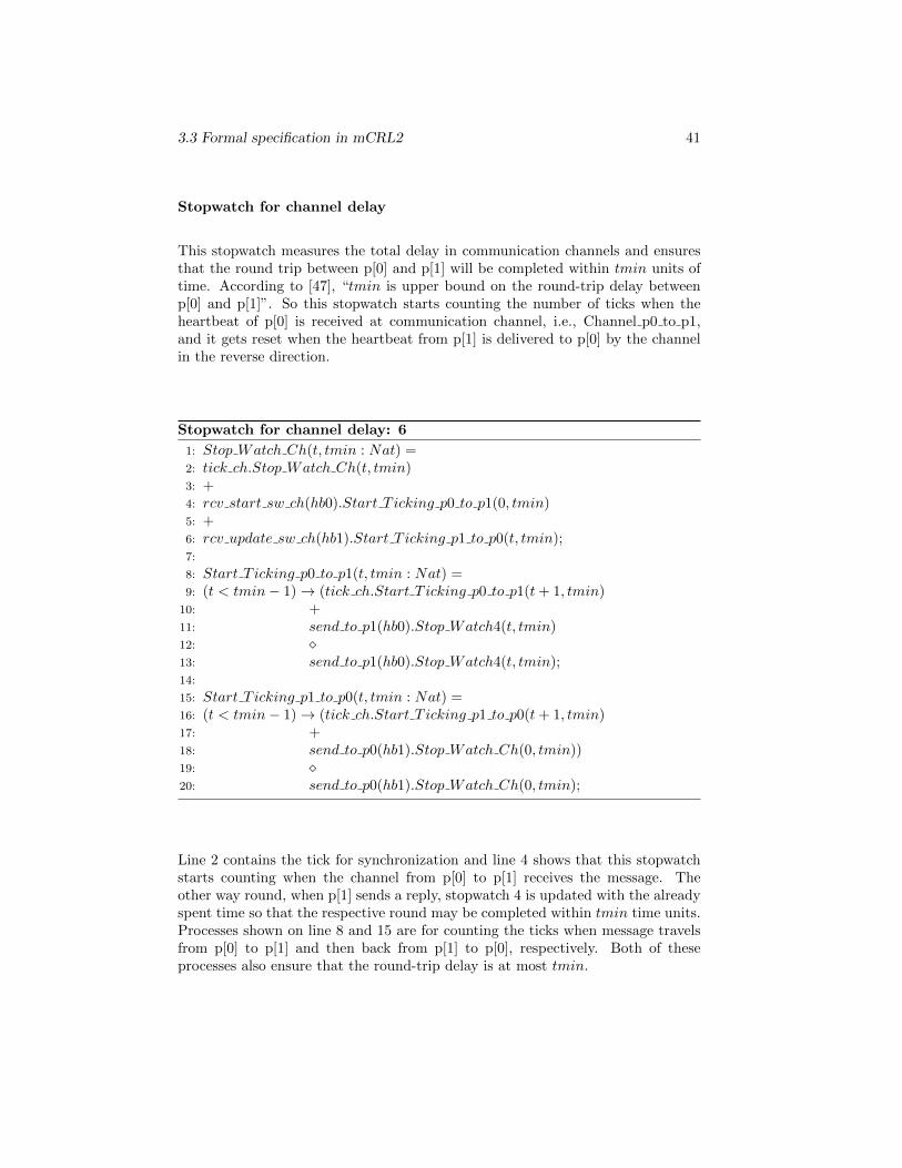
3.3 Formal specification in mCRL2 41
Stopwatch for channel delay
This stopwatch measures the total delay in communication channels and ensuresthat the round trip between p[0] and p[1] will be completed within tmin units oftime. According to [47], “tmin is upper bound on the round-trip delay betweenp[0] and p[1]”. So this stopwatch starts counting the number of ticks when theheartbeat of p[0] is received at communication channel, i.e., Channel p0 to p1,and it gets reset when the heartbeat from p[1] is delivered to p[0] by the channelin the reverse direction.
Stopwatch for channel delay: 6
1: Stop Watch Ch(t, tmin : Nat) =2: tick ch.Stop Watch Ch(t, tmin)3: +4: rcv start sw ch(hb0).Start T icking p0 to p1(0, tmin)5: +6: rcv update sw ch(hb1).Start T icking p1 to p0(t, tmin);7:
8: Start T icking p0 to p1(t, tmin : Nat) =9: (t < tmin− 1)→ (tick ch.Start T icking p0 to p1(t+ 1, tmin)
10: +11: send to p1(hb0).Stop Watch4(t, tmin)12: �13: send to p1(hb0).Stop Watch4(t, tmin);14:
15: Start T icking p1 to p0(t, tmin : Nat) =16: (t < tmin− 1)→ (tick ch.Start T icking p1 to p0(t+ 1, tmin)17: +18: send to p0(hb1).Stop Watch Ch(0, tmin))19: �20: send to p0(hb1).Stop Watch Ch(0, tmin);
Line 2 contains the tick for synchronization and line 4 shows that this stopwatchstarts counting when the channel from p[0] to p[1] receives the message. Theother way round, when p[1] sends a reply, stopwatch 4 is updated with the alreadyspent time so that the respective round may be completed within tmin time units.Processes shown on line 8 and 15 are for counting the ticks when message travelsfrom p[0] to p[1] and then back from p[1] to p[0], respectively. Both of theseprocesses also ensure that the round-trip delay is at most tmin.
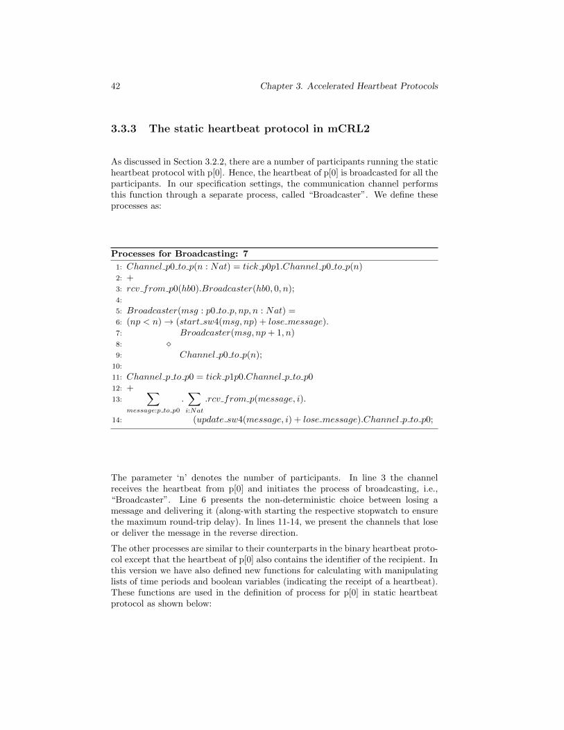
42 Chapter 3. Accelerated Heartbeat Protocols
3.3.3 The static heartbeat protocol in mCRL2
As discussed in Section 3.2.2, there are a number of participants running the staticheartbeat protocol with p[0]. Hence, the heartbeat of p[0] is broadcasted for all theparticipants. In our specification settings, the communication channel performsthis function through a separate process, called “Broadcaster”. We define theseprocesses as:
Processes for Broadcasting: 7
1: Channel p0 to p(n : Nat) = tick p0p1.Channel p0 to p(n)2: +3: rcv from p0(hb0).Broadcaster(hb0, 0, n);4:
5: Broadcaster(msg : p0 to p, np, n : Nat) =6: (np < n)→ (start sw4(msg, np) + lose message).7: Broadcaster(msg, np+ 1, n)8: �9: Channel p0 to p(n);
10:
11: Channel p to p0 = tick p1p0.Channel p to p012: +13:
∑message:p to p0
.∑i:Nat
.rcv from p(message, i).
14: (update sw4(message, i) + lose message).Channel p to p0;
The parameter ‘n’ denotes the number of participants. In line 3 the channelreceives the heartbeat from p[0] and initiates the process of broadcasting, i.e.,“Broadcaster”. Line 6 presents the non-deterministic choice between losing amessage and delivering it (along-with starting the respective stopwatch to ensurethe maximum round-trip delay). In lines 11-14, we present the channels that loseor deliver the message in the reverse direction.
The other processes are similar to their counterparts in the binary heartbeat proto-col except that the heartbeat of p[0] also contains the identifier of the recipient. Inthis version we have also defined new functions for calculating with manipulatinglists of time periods and boolean variables (indicating the receipt of a heartbeat).These functions are used in the definition of process for p[0] in static heartbeatprotocol as shown below:
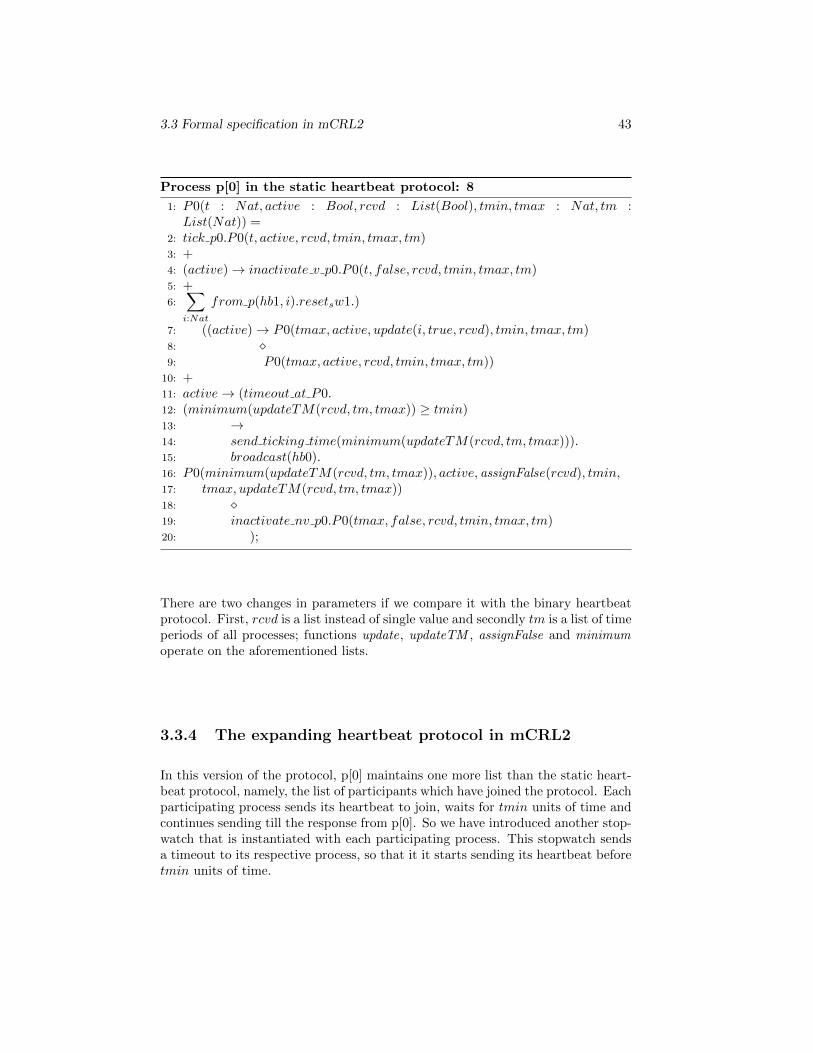
3.3 Formal specification in mCRL2 43
Process p[0] in the static heartbeat protocol: 8
1: P0(t : Nat, active : Bool, rcvd : List(Bool), tmin, tmax : Nat, tm :List(Nat)) =
2: tick p0.P0(t, active, rcvd, tmin, tmax, tm)3: +4: (active)→ inactivate v p0.P0(t, false, rcvd, tmin, tmax, tm)5: +6:
∑i:Nat
from p(hb1, i).resetsw1.)
7: ((active)→ P0(tmax, active, update(i, true, rcvd), tmin, tmax, tm)8: �9: P0(tmax, active, rcvd, tmin, tmax, tm))
10: +11: active→ (timeout at P0.12: (minimum(updateTM(rcvd, tm, tmax)) ≥ tmin)13: →14: send ticking time(minimum(updateTM(rcvd, tm, tmax))).15: broadcast(hb0).16: P0(minimum(updateTM(rcvd, tm, tmax)), active, assignFalse(rcvd), tmin,17: tmax, updateTM(rcvd, tm, tmax))18: �19: inactivate nv p0.P0(tmax, false, rcvd, tmin, tmax, tm)20: );
There are two changes in parameters if we compare it with the binary heartbeatprotocol. First, rcvd is a list instead of single value and secondly tm is a list of timeperiods of all processes; functions update, updateTM , assignFalse and minimumoperate on the aforementioned lists.
3.3.4 The expanding heartbeat protocol in mCRL2
In this version of the protocol, p[0] maintains one more list than the static heart-beat protocol, namely, the list of participants which have joined the protocol. Eachparticipating process sends its heartbeat to join, waits for tmin units of time andcontinues sending till the response from p[0]. So we have introduced another stop-watch that is instantiated with each participating process. This stopwatch sendsa timeout to its respective process, so that it it starts sending its heartbeat beforetmin units of time.
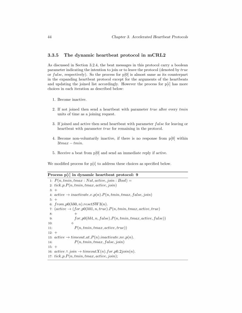
44 Chapter 3. Accelerated Heartbeat Protocols
3.3.5 The dynamic heartbeat protocol in mCRL2
As discussed in Section 3.2.4, the beat messages in this protocol carry a booleanparameter indicating the intention to join or to leave the protocol (denoted by trueor false, respectively). So the process for p[0] is almost same as its counterpartin the expanding heartbeat protocol except for the arguments of the heartbeatsand updating the joined list accordingly. However the process for p[i] has morechoices in each iteration as described below:
1. Become inactive.
2. If not joined then send a heartbeat with parameter true after every tminunits of time as a joining request.
3. If joined and active then send heartbeat with parameter false for leaving orheartbeat with parameter true for remaining in the protocol.
4. Become non-voluntarily inactive, if there is no response from p[0] within3tmax− tmin.
5. Receive a beat from p[0] and send an immediate reply if active.
We modified process for p[i] to address these choices as specified below.
Process p[i] in dynamic heartbeat protocol: 9
1: P (n, tmin, tmax : Nat, active, join : Bool) =2: tick p.P (n, tmin, tmax, active, join)3: +4: active→ inactivate v p(n).P (n, tmin, tmax, false, join)5: +6: from p0(hb0, n).resetSW3(n).7: (active→ (for p0(hb1, n, true).P (n, tmin, tmax, active, true)8: +9: for p0(hb1, n, false).P (n, tmin, tmax, active, false))
10: �11: P (n, tmin, tmax, active, true))12: +13: active→ timeout at P (n).inactivate nv p(n).14: P (n, tmin, tmax, false, join)15: +16: active ∧ join→ timeoutX(n).for p0 2join(n).17: tick p.P (n, tmin, tmax, active, join);
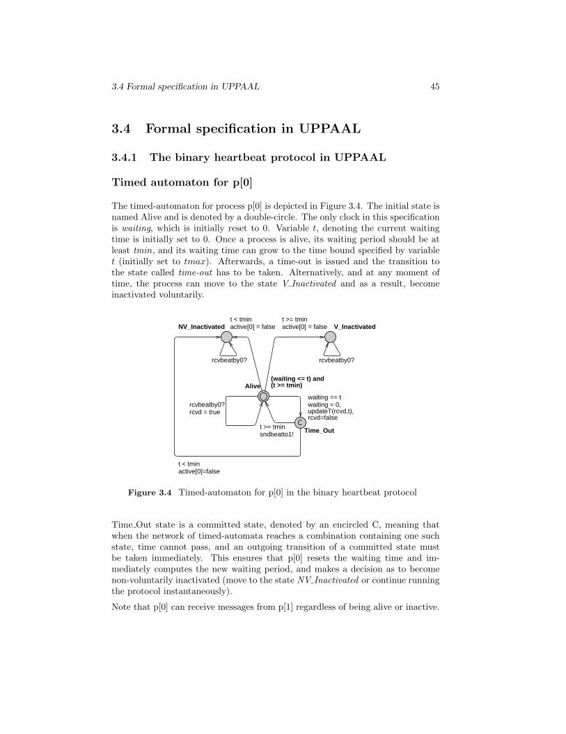
3.4 Formal specification in UPPAAL 45
3.4 Formal specification in UPPAAL
3.4.1 The binary heartbeat protocol in UPPAAL
Timed automaton for p[0]
The timed-automaton for process p[0] is depicted in Figure 3.4. The initial state isnamed Alive and is denoted by a double-circle. The only clock in this specificationis waiting, which is initially reset to 0. Variable t, denoting the current waitingtime is initially set to 0. Once a process is alive, its waiting period should be atleast tmin, and its waiting time can grow to the time bound specified by variablet (initially set to tmax). Afterwards, a time-out is issued and the transition tothe state called time-out has to be taken. Alternatively, and at any moment oftime, the process can move to the state V Inactivated and as a result, becomeinactivated voluntarily.
Time_Out
NV_Inactivated V_Inactivated
Alive(waiting <= t) and (t >= tmin)
rcvbeatby0?
t >= tminsndbeatto1!
t < tminactive[0]=false
waiting == twaiting = 0,updateT(rcvd,t),rcvd=false
rcvbeatby0?
t < tminactive[0] = false
rcvbeatby0?rcvd = true
t >= tminactive[0] = false
Figure 3.4 Timed-automaton for p[0] in the binary heartbeat protocol
Time Out state is a committed state, denoted by an encircled C, meaning thatwhen the network of timed-automata reaches a combination containing one suchstate, time cannot pass, and an outgoing transition of a committed state mustbe taken immediately. This ensures that p[0] resets the waiting time and im-mediately computes the new waiting period, and makes a decision as to becomenon-voluntarily inactivated (move to the state NV Inactivated or continue runningthe protocol instantaneously).
Note that p[0] can receive messages from p[1] regardless of being alive or inactive.
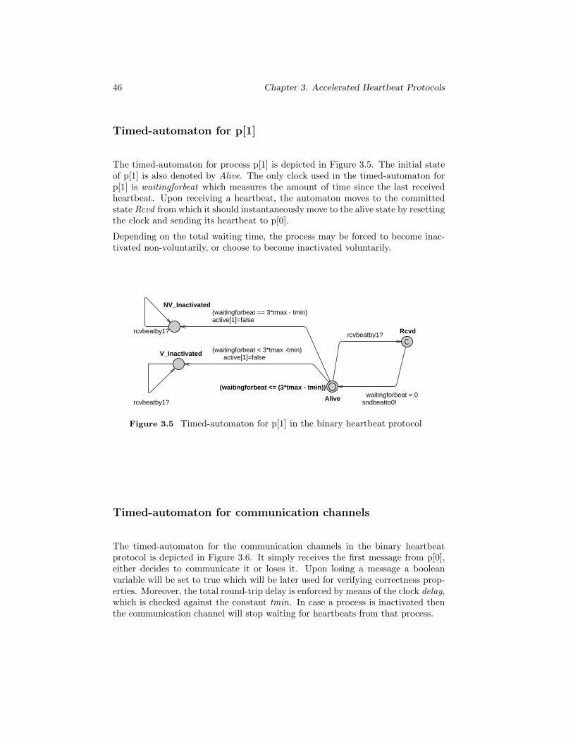
46 Chapter 3. Accelerated Heartbeat Protocols
Timed-automaton for p[1]
The timed-automaton for process p[1] is depicted in Figure 3.5. The initial stateof p[1] is also denoted by Alive. The only clock used in the timed-automaton forp[1] is waitingforbeat which measures the amount of time since the last receivedheartbeat. Upon receiving a heartbeat, the automaton moves to the committedstate Rcvd from which it should instantaneously move to the alive state by resettingthe clock and sending its heartbeat to p[0].
Depending on the total waiting time, the process may be forced to become inac-tivated non-voluntarily, or choose to become inactivated voluntarily.
NV_Inactivated
Rcvd
V_Inactivated
Alive
(waitingforbeat <= (3*tmax - tmin))
rcvbeatby1?
rcvbeatby1?
(waitingforbeat < 3*tmax -tmin)active[1]=false
(waitingforbeat == 3*tmax - tmin)active[1]=false
sndbeatto0!waitingforbeat = 0
rcvbeatby1?
Figure 3.5 Timed-automaton for p[1] in the binary heartbeat protocol
Timed-automaton for communication channels
The timed-automaton for the communication channels in the binary heartbeatprotocol is depicted in Figure 3.6. It simply receives the first message from p[0],either decides to communicate it or loses it. Upon losing a message a booleanvariable will be set to true which will be later used for verifying correctness prop-erties. Moreover, the total round-trip delay is enforced by means of the clock delay,which is checked against the constant tmin. In case a process is inactivated thenthe communication channel will stop waiting for heartbeats from that process.
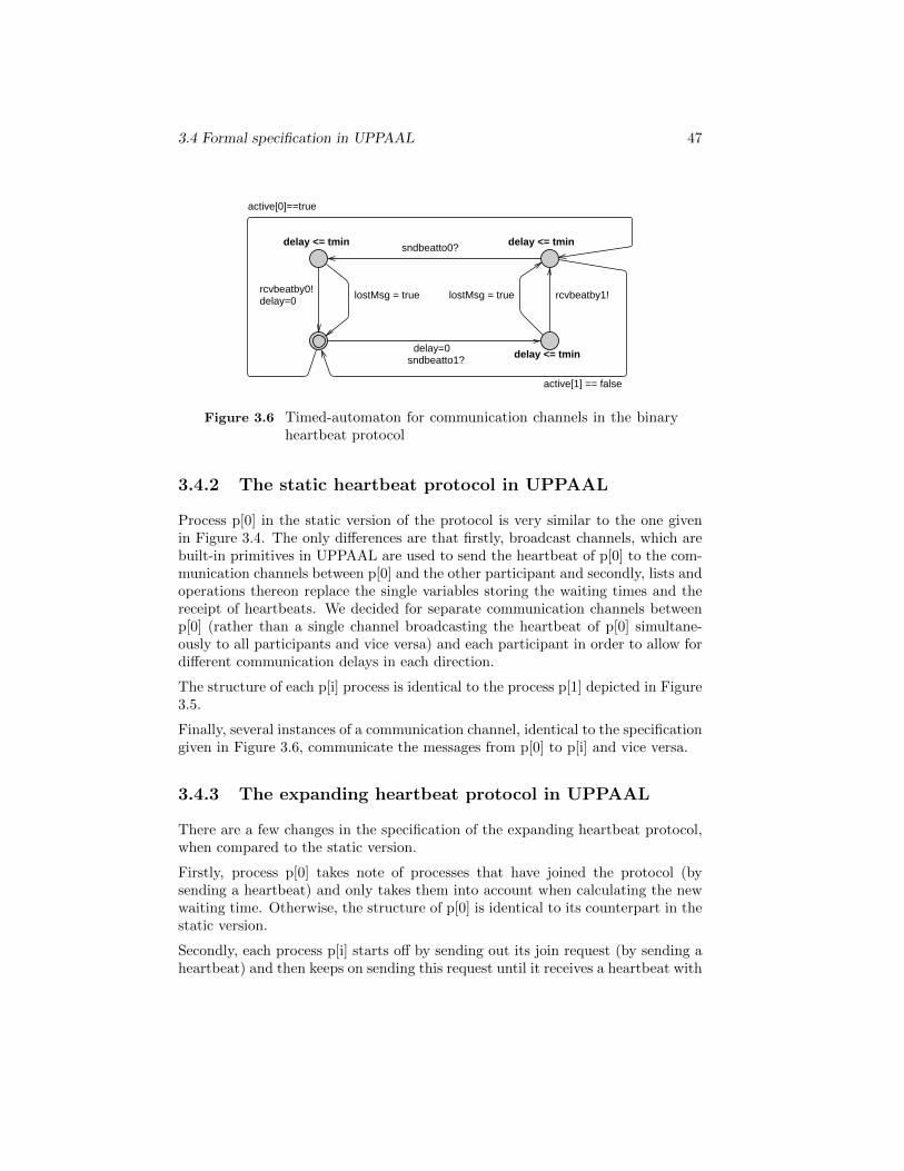
3.4 Formal specification in UPPAAL 47
delay <= tmin delay <= tmin
delay <= tmin
active[0]==true
lostMsg = true lostMsg = true
active[1] == false
rcvbeatby0!delay=0
sndbeatto0?
rcvbeatby1!
sndbeatto1?delay=0
Figure 3.6 Timed-automaton for communication channels in the binaryheartbeat protocol
3.4.2 The static heartbeat protocol in UPPAAL
Process p[0] in the static version of the protocol is very similar to the one givenin Figure 3.4. The only differences are that firstly, broadcast channels, which arebuilt-in primitives in UPPAAL are used to send the heartbeat of p[0] to the com-munication channels between p[0] and the other participant and secondly, lists andoperations thereon replace the single variables storing the waiting times and thereceipt of heartbeats. We decided for separate communication channels betweenp[0] (rather than a single channel broadcasting the heartbeat of p[0] simultane-ously to all participants and vice versa) and each participant in order to allow fordifferent communication delays in each direction.
The structure of each p[i] process is identical to the process p[1] depicted in Figure3.5.
Finally, several instances of a communication channel, identical to the specificationgiven in Figure 3.6, communicate the messages from p[0] to p[i] and vice versa.
3.4.3 The expanding heartbeat protocol in UPPAAL
There are a few changes in the specification of the expanding heartbeat protocol,when compared to the static version.
Firstly, process p[0] takes note of processes that have joined the protocol (bysending a heartbeat) and only takes them into account when calculating the newwaiting time. Otherwise, the structure of p[0] is identical to its counterpart in thestatic version.
Secondly, each process p[i] starts off by sending out its join request (by sending aheartbeat) and then keeps on sending this request until it receives a heartbeat with
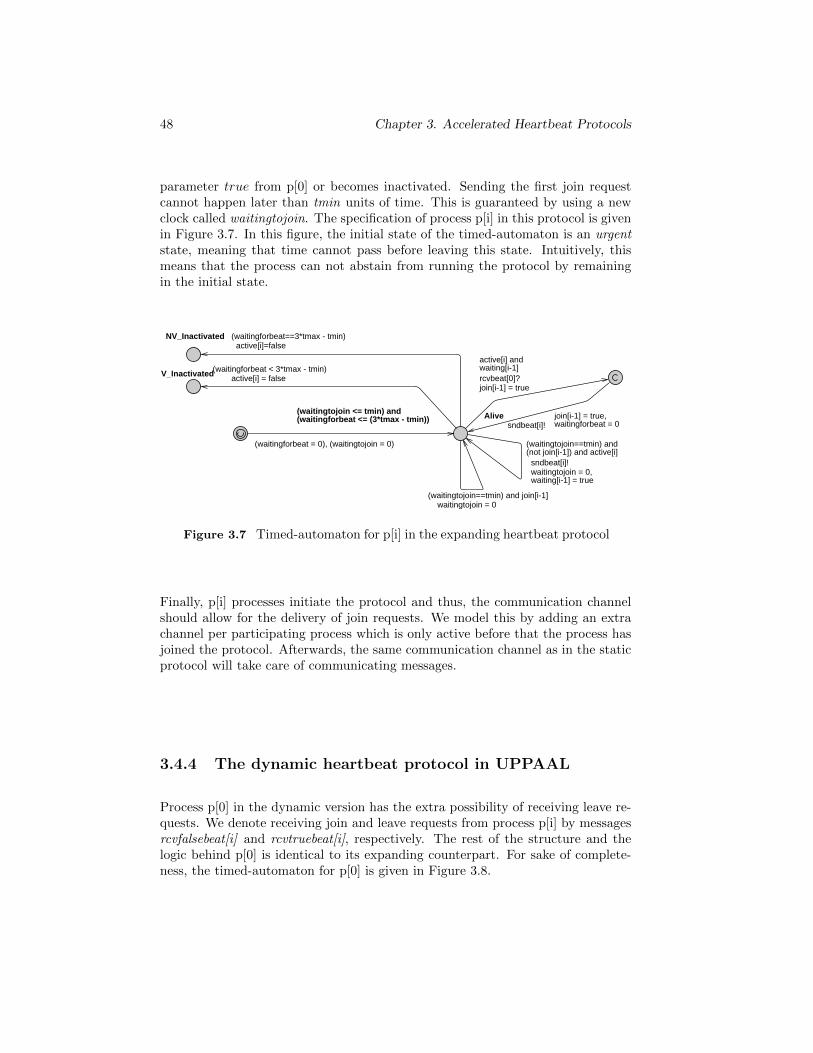
48 Chapter 3. Accelerated Heartbeat Protocols
parameter true from p[0] or becomes inactivated. Sending the first join requestcannot happen later than tmin units of time. This is guaranteed by using a newclock called waitingtojoin. The specification of process p[i] in this protocol is givenin Figure 3.7. In this figure, the initial state of the timed-automaton is an urgentstate, meaning that time cannot pass before leaving this state. Intuitively, thismeans that the process can not abstain from running the protocol by remainingin the initial state.
NV_Inactivated
V_Inactivated
Alive(waitingtojoin <= tmin) and (waitingforbeat <= (3*tmax - tmin))
(waitingforbeat==3*tmax - tmin)active[i]=false
sndbeat[i]!join[i-1] = true, waitingforbeat = 0
active[i] and waiting[i-1]rcvbeat[0]?join[i-1] = true
(waitingtojoin==tmin) and join[i-1]waitingtojoin = 0
(waitingtojoin==tmin) and (not join[i-1]) and active[i]
sndbeat[i]!waitingtojoin = 0,waiting[i-1] = true
(waitingforbeat = 0), (waitingtojoin = 0)
(waitingforbeat < 3*tmax - tmin)active[i] = false
Figure 3.7 Timed-automaton for p[i] in the expanding heartbeat protocol
Finally, p[i] processes initiate the protocol and thus, the communication channelshould allow for the delivery of join requests. We model this by adding an extrachannel per participating process which is only active before that the process hasjoined the protocol. Afterwards, the same communication channel as in the staticprotocol will take care of communicating messages.
3.4.4 The dynamic heartbeat protocol in UPPAAL
Process p[0] in the dynamic version has the extra possibility of receiving leave re-quests. We denote receiving join and leave requests from process p[i] by messagesrcvfalsebeat[i] and rcvtruebeat[i], respectively. The rest of the structure and thelogic behind p[0] is identical to its expanding counterpart. For sake of complete-ness, the timed-automaton for p[0] is given in Figure 3.8.
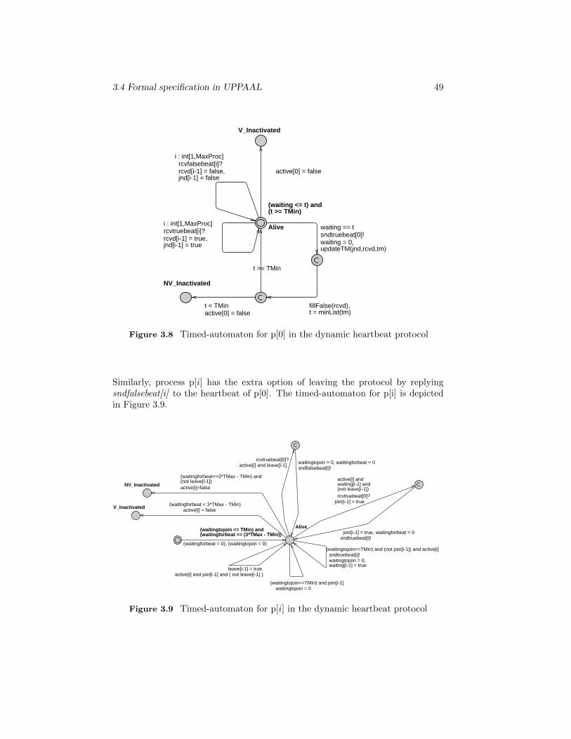
3.4 Formal specification in UPPAAL 49
NV_Inactivated
V_Inactivated
Alive
(waiting <= t) and (t >= TMin)
t < TMinactive[0] = false
t >= TMin
fillFalse(rcvd),t = minList(tm)
waiting == tsndtruebeat[0]!waiting = 0,updateTM(jnd,rcvd,tm)
i : int[1,MaxProc]rcvfalsebeat[i]?rcvd[i-1] = false, jnd[i-1] = false
i : int[1,MaxProc]rcvtruebeat[i]?rcvd[i-1] = true, jnd[i-1] = true
active[0] = false
Figure 3.8 Timed-automaton for p[0] in the dynamic heartbeat protocol
Similarly, process p[i] has the extra option of leaving the protocol by replyingsndfalsebeat[i] to the heartbeat of p[0]. The timed-automaton for p[i] is depictedin Figure 3.9.
NV_Inactivated
V_Inactivated
Alive(waitingtojoin <= TMin) and (waitingforbeat <= (3*TMax - TMin))
(waitingforbeat==3*TMax - TMin) and (not leave[i-1])active[i]=false
sndfalsebeat[i]!waitingtojoin = 0, waitingforbeat = 0active[i] and leave[i-1]
rcvtruebeat[0]?
sndtruebeat[i]!join[i-1] = true, waitingforbeat = 0
active[i] and waiting[i-1] and (not leave[i-1])rcvtruebeat[0]?
join[i-1] = true
active[i] and join[i-1] and ( not leave[i-1] )leave[i-1] = true
(waitingtojoin==TMin) and join[i-1]waitingtojoin = 0
(waitingtojoin==TMin) and (not join[i-1]) and active[i]sndtruebeat[i]!waitingtojoin = 0,waiting[i-1] = true
(waitingforbeat = 0), (waitingtojoin = 0)
(waitingforbeat < 3*TMax - TMin)active[i] = false
Figure 3.9 Timed-automaton for p[i] in the dynamic heartbeat protocol
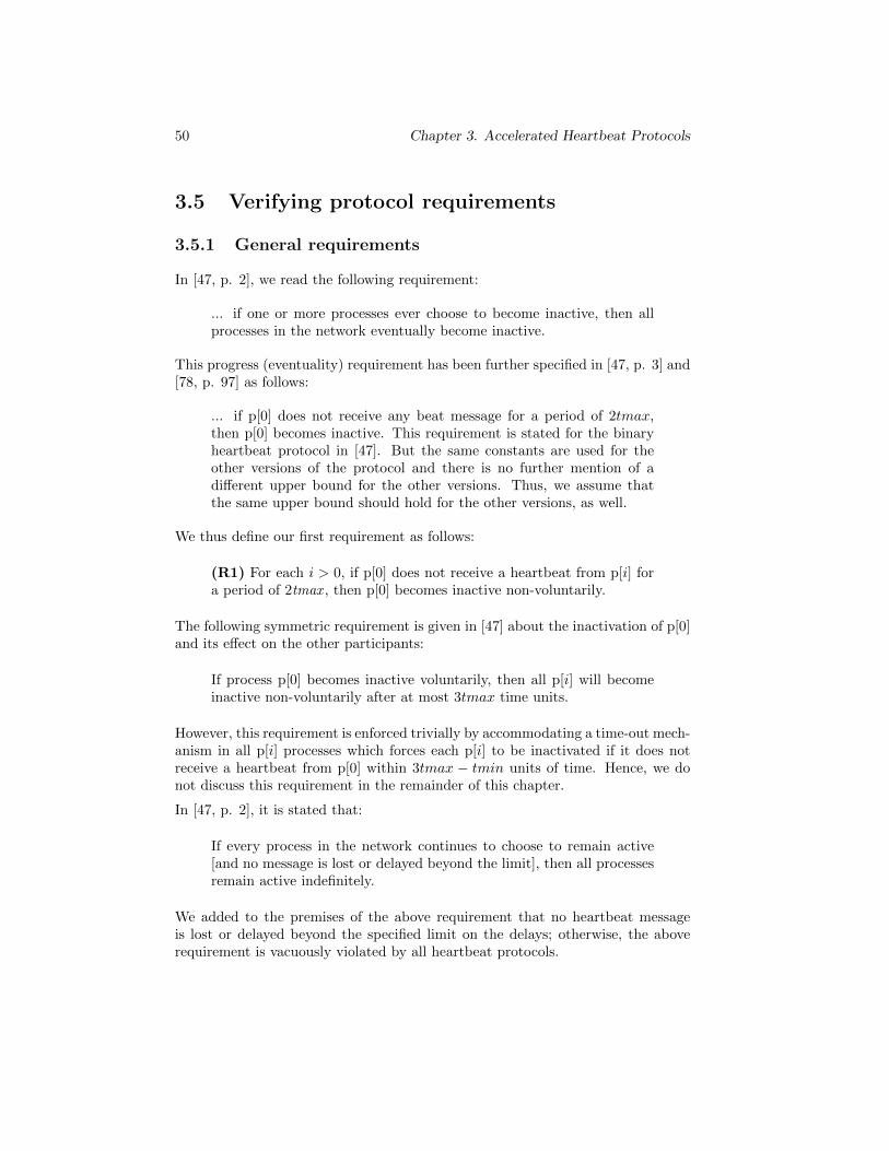
50 Chapter 3. Accelerated Heartbeat Protocols
3.5 Verifying protocol requirements
3.5.1 General requirements
In [47, p. 2], we read the following requirement:
... if one or more processes ever choose to become inactive, then allprocesses in the network eventually become inactive.
This progress (eventuality) requirement has been further specified in [47, p. 3] and[78, p. 97] as follows:
... if p[0] does not receive any beat message for a period of 2tmax,then p[0] becomes inactive. This requirement is stated for the binaryheartbeat protocol in [47]. But the same constants are used for theother versions of the protocol and there is no further mention of adifferent upper bound for the other versions. Thus, we assume thatthe same upper bound should hold for the other versions, as well.
We thus define our first requirement as follows:
(R1) For each i > 0, if p[0] does not receive a heartbeat from p[i] fora period of 2tmax , then p[0] becomes inactive non-voluntarily.
The following symmetric requirement is given in [47] about the inactivation of p[0]and its effect on the other participants:
If process p[0] becomes inactive voluntarily, then all p[i] will becomeinactive non-voluntarily after at most 3tmax time units.
However, this requirement is enforced trivially by accommodating a time-out mech-anism in all p[i] processes which forces each p[i] to be inactivated if it does notreceive a heartbeat from p[0] within 3tmax − tmin units of time. Hence, we donot discuss this requirement in the remainder of this chapter.
In [47, p. 2], it is stated that:
If every process in the network continues to choose to remain active[and no message is lost or delayed beyond the limit], then all processesremain active indefinitely.
We added to the premises of the above requirement that no heartbeat messageis lost or delayed beyond the specified limit on the delays; otherwise, the aboverequirement is vacuously violated by all heartbeat protocols.
3.5 Verifying protocol requirements 51
(R2, R3) For each i ≥ 0, if there has been no voluntary inactivationof any p[j] (for each i 6= j) and no message is lost or delayed beyondits limit, then p[i] is not inactivated non-voluntarily.
We split the above statement into two requirement (R2) and (R3). For eachi > 0, (R2) requires that as long as p[0] and all p[j], where j ≥ 0 and j 6= i,are active, and all channels are up, the protocol should not inactivate p[i] non-voluntarily. Requirement (R3) specifies that if all p[j] processes, where j > 0,are active and all channels are up, then the protocol should not inactivate p[0]non-voluntarily.
3.5.2 Formalizing the requirements in the modal µ-calculus
R1. To formalize the progress requirement (R1), we devised a watchdog for eachprocess p[i], which starts counting down from 2tmax and is reset by eachheartbeat of p[i] received at p[0]. All watchdogs are inactivated when p[0]is non-voluntarily inactivated. If a watchdog reaches 0 and does not receivean inactivation message from p[0] before the next time unit, it will issue aspecial message called “error”. (In case of expanding and dynamic protocols,the watchdog of p[i] is only active after that the first joining request, i.e., aheartbeat with parameter true, is sent by p[i] and in the dynamic protocol, itremains active until a leave request is sent by p[i].) Then, we use the followingsimple formula in the modal µ-calculus, for checking the reachability of atrace containing an action error .
[true∗.error ]false
The notation [r]φ, where r is a regular expression over actions and φ is a for-mula, specifies that after all traces satisfying r, φ should hold. Particularly,[r]false specifies that no trace satisfying r is reachable (since otherwise falseshould be satisfied, which is impossible).
R2. For the binary and static versions of this protocol, the formalization of thisrequirement is straightforward. Namely, for each i > 0, the following formulaformalizes requirement (R2).
[(∧
j≥0,i6=jinactivate v p(j) ∧ lose msg)∗.inactivate nv p(i)]false
The above formula states that non-voluntary inactivation of p[i], denoted byaction inactivate nv p(i), is always preceded by a voluntary inactivation ofanother process p[j], denoted by action inactivate v p(j), or a message loss,denoted by action lose msg.
52 Chapter 3. Accelerated Heartbeat Protocols
However, for the expanding and dynamic protocols, the above formula is tooweak. It disregards joining and leaving requests and for example, allows for aprocess which has not joined, or joined but then left the protocol to becomenon-voluntarily inactive. Next, we give the formalization of this requirementin modal µ-calculus for the dynamic protocol and for three participants:
[p joined(1 )∗.inactivate nv p(1 )]false∧
[nofault({0})∗.p left(2 ).nofault({0})∗.inactivate nv p(1 )]false∧[nofault({0 , 2})∗.inactivate nv p(1 )]false,
where nofault(I ) stands forlose msg∧∧i∈I(inactivate v p(0)∧ inactivate nv p(0)) and p left(2 ) standsfor sent by p[2 ](false). true∗. rcv from p[0 ](true). This formula states thatp[1] is not allowed to be non-voluntarily inactivated, if it has not joinedthe protocol, or if it has joined, no other process has joined and no faulthas occurred in p[0] or the channel, or if no fault has occurred in p[0], theparticipants and the channel.
R3. The following formula formalizes requirement (R3), which states that non-voluntary inactivation of p[0] must be preceded with the voluntary inactiva-tion of some p[i] (for some i > 0) or a message loss.
[(∧i>0
inactivate v p(i) ∧ lose msg)∗.inactivate nv p(0)]false
As in requirement R2, the formalizations of R3 for the expanding and thedynamic protocols are more involved.
[(∧i>0 p joined(i))
∗.inactivate nv p0 ]false∧
[noinact({1})∗.p left(2 ).noinact(1 )∗.inactivate nv p(1 )]false∧
[noinact({0 , 1})∗.inactivate nv p(1 )]false,
where noinact(I ) stands for lose msg ∧∧i∈I inactivate v p(0).
3.5.3 Formalizing the requirements in UPPAAL
R1. To formalize requirement R1, we devise a timed-automaton that runs inparallel with the protocol and observes the receipt of heartbeats and thethe corresponding inactivation. If it is observed that despite not receivinga heartbeat for 2tmax , the monitor processes for the binary and dynamicprotocols are given, respectively, in Figures 3.10.(a) and 3.10.(b).
Subsequently, requirement R1 for the binary protocol is formalized in UP-PAAL in terms of (the negation of) the following reachability property:
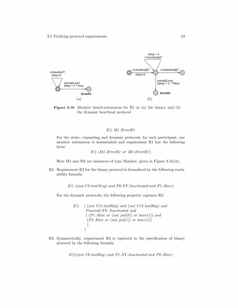
3.5 Verifying protocol requirements 53
ErrorR1
active[0] and delay > 2 * tmax
rcvbeatby0?delay=0
ErrorR1
active[0] and (delay > 2 * TMax)
rcvtruebeat[i]?
delay=0
rcvfalsebeat[i]?
rcvtruebeat[i]?delay = 0
(a) (b)
Figure 3.10 Monitor timed-automaton for R1 in (a) the binary and (b)the dynamic heartbeat protocol
E♦ M1 .ErrorR1
For the static, expanding and dynamic protocols, for each participant, onemonitor automaton is instantiated and requirement R1 has the followingform:
E♦ (M1 .ErrorR1 or M2 .ErrorR1 )
Here M1 and M2 are instances of type Monitor, given in Figure 3.10.(b).
R2. Requirement R2 for the binary protocol is formalized by the following reach-ability formula:
E♦ ((not Ch.lostMsg) and P0.NV Inactivated and P1.Alive)
For the dynamic protocols, the following property captures R2:
E♦ ( (not C11 .lostMsg) and (not C12 .lostMsg) andProcess0 .NV Inactivated and( (P1 .Alive or (not jnd [0 ]) or leave[1 ]) and(P2 .Alive or (not jnd [1 ]) or leave[1 ]))
)
R3. Symmetrically, requirement R3 is captured in the specification of binaryprotocol by the following formula:
E♦((not Ch.lostMsg) and P1 .NV Inactivated and P0 .Alive)
54 Chapter 3. Accelerated Heartbeat Protocols
For the dynamic protocol, the requirement is specified in terms of the fol-lowing formula:
E♦ ((not C11 .lostMsg) and (not C12 .lostMsg) and P1 .NV Inactivatedand (Process0 .Alive and (P2 .Alive or (not jnd [1 ]))))
3.5.4 Verification techniques
We applied model checking techniques for the verification of R1, R2 and R3(discussed in Section 3.5.2) with respect to the different versions of acceleratedheartbeat protocols. We used the process algebra mCRL2 [50] for modeling andevaluated the formulae with model checker CADP [45]. In the process algebraicapproach, a number of steps should be taken between modeling (with mCRL2) andmodel checking (with CADP). Namely, we translated the models to the respectivelinear process specifications (LPS) [52] (a simple format used for storing and ma-nipulating recursive process definitions). From the LPS, we generated the statespace after applying different state space reduction techniques, such as minimiz-ing modulo strong bisimilarity and eliminating constants, superfluous summandsand inconsequential parameters. We also modeled the same protocols in timed-automata and used UPPAAL [72] to verify the properties specified in Section 3.5.3.Both model checkers produced similar results.
3.5.5 Verification results
We used different data sets for tmin and tmax for each protocol presented in [47]and [78]. (Note that the only constraint on tmin and tmax according to [47] isthat 0 < tmin ≤ tmax .) Since the counterexamples reported for the (revised)binary, two-phase and static heartbeat protocols are identical, we report aboutthem once.1
1For the two-phase heartbeat protocol the condition for non-voluntary inactivation of p[0] isnot specified in [47]. Hence, we could not verify properties (R1) and (R3) for this version of theprotocol.
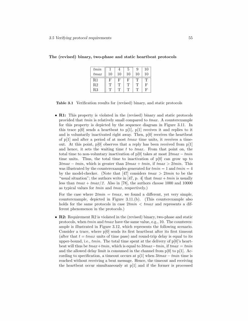
3.5 Verifying protocol requirements 55
The (revised) binary, two-phase and static heartbeat protocols
tmin 1 4 5 9 10tmax 10 10 10 10 10
R1 F F F T TR2 T T T T FR3 T T T T F
Table 3.1 Verification results for (revised) binary, and static protocols
• R1: This property is violated in the (revised) binary and static protocolsprovided that tmin is relatively small compared to tmax . A counterexamplefor this property is depicted by the sequence diagram in Figure 3.11. Inthis trace p[0] sends a heartbeat to p[1], p[1] receives it and replies to itand is voluntarily inactivated right away. Then, p[0] receives the heartbeatof p[1] and after a period of at most tmax time units, it receives a time-out. At this point, p[0] observes that a reply has been received from p[1]and hence, it sets the waiting time t to tmax . From that point on, thetotal time to non-voluntary inactivation of p[0] takes at most 2tmax − tmintime units. Thus, the total time to inactivation of p[0] can grow up to3tmax − tmin, which is greater than 2tmax + tmin, if tmax > 2tmin. Thiswas illustrated by the counterexamples generated for tmin = 1 and tmin = 4by the model-checker. (Note that [47] considers tmax > 2tmin to be the“usual situation”; the authors write in [47, p. 4] that tmax + tmin is usuallyless than tmax + tmax/2 . Also in [78], the authors choose 1000 and 10000as typical values for tmin and tmax , respectively.)
For the case where 2tmin = tmax, we found a different, yet very simple,counterexample, depicted in Figure 3.11.(b). (This counterexample alsoholds for the same protocols in case 2tmin < tmax and represents a dif-ferent phenomenon in the protocols.)
• R2: Requirement R2 is violated in the (revised) binary, two-phase and staticprotocols, when tmin and tmax have the same value, e.g., 10. The counterex-ample is illustrated in Figure 3.12, which represents the following scenario.Consider a trace, where p[0] sends its first heartbeat after its first timeout(after that t = tmax units of time pass) and round-trip delay is equal to itsupper-bound, i.e., tmin. The total time spent at the delivery of p[0]’s heart-beat will thus be tmax +tmin, which is equal to 3tmax−tmin, if tmax = tminand the allowed delay limit is consumed in the channel from p[0] to p[1]. Ac-cording to specification, a timeout occurs at p[1] when 3tmax − tmin time isreached without receiving a beat message. Hence, the timeout and receivingthe heartbeat occur simultaneously at p[1] and if the former is processed
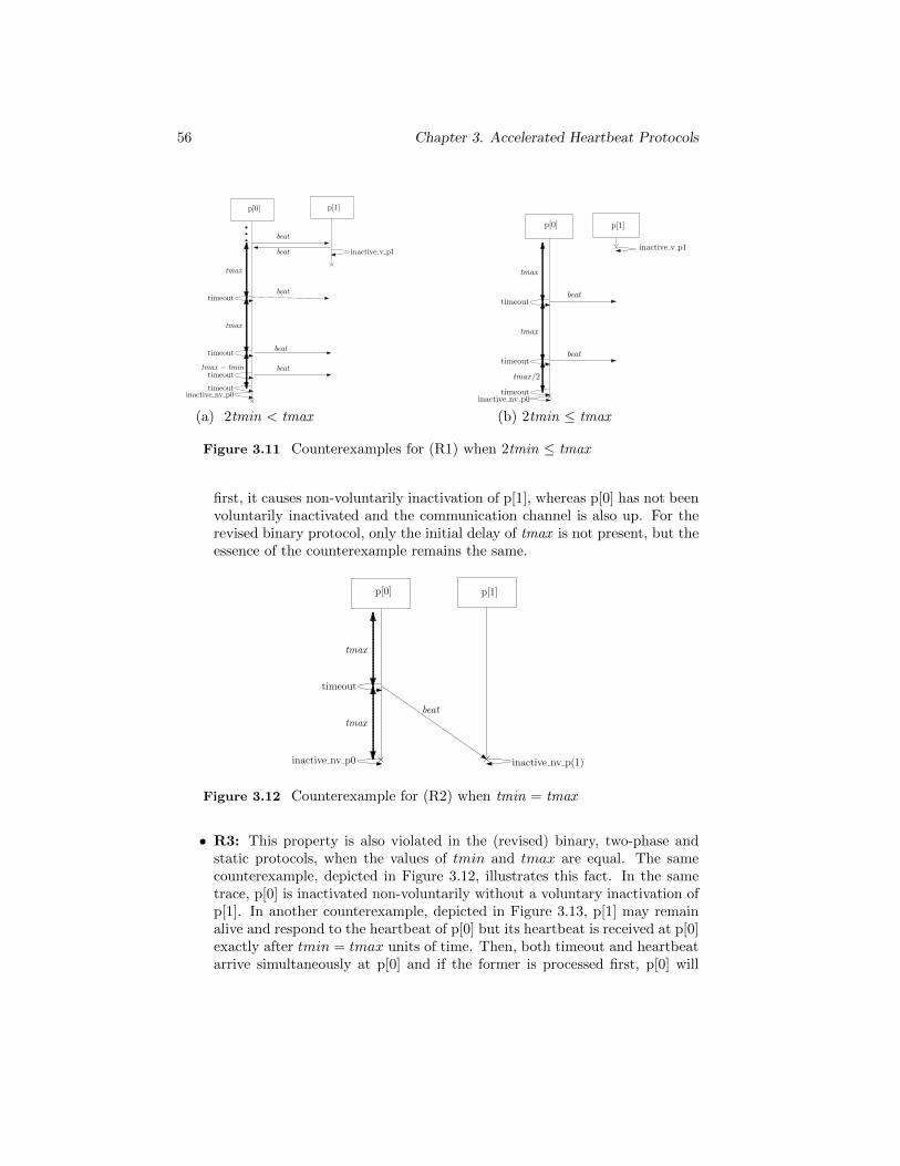
56 Chapter 3. Accelerated Heartbeat Protocols
p[0]
timeout
p[1]
tmax
tmax
inactive v p1
tmax − tmin
timeout
timeout
timeoutinactive nv p0
beat
beat
beat
beat
beat
p[0]
timeout
p[1]
tmax
tmax
beat
timeout
inactive v p1
tmax/2
timeout
beat
inactive nv p0
(a) 2tmin < tmax (b) 2tmin ≤ tmax
Figure 3.11 Counterexamples for (R1) when 2tmin ≤ tmax
first, it causes non-voluntarily inactivation of p[1], whereas p[0] has not beenvoluntarily inactivated and the communication channel is also up. For therevised binary protocol, only the initial delay of tmax is not present, but theessence of the counterexample remains the same.
p[0]
timeout
p[1]
tmax
tmax
inactive nv p(1)inactive nv p0
beat
Figure 3.12 Counterexample for (R2) when tmin = tmax
• R3: This property is also violated in the (revised) binary, two-phase andstatic protocols, when the values of tmin and tmax are equal. The samecounterexample, depicted in Figure 3.12, illustrates this fact. In the sametrace, p[0] is inactivated non-voluntarily without a voluntary inactivation ofp[1]. In another counterexample, depicted in Figure 3.13, p[1] may remainalive and respond to the heartbeat of p[0] but its heartbeat is received at p[0]exactly after tmin = tmax units of time. Then, both timeout and heartbeatarrive simultaneously at p[0] and if the former is processed first, p[0] will
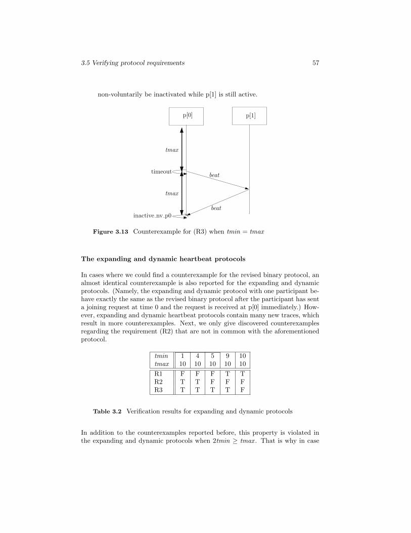
3.5 Verifying protocol requirements 57
non-voluntarily be inactivated while p[1] is still active.
p[0]
timeout
p[1]
tmax
tmax
inactive nv p0
beat
beat
Figure 3.13 Counterexample for (R3) when tmin = tmax
The expanding and dynamic heartbeat protocols
In cases where we could find a counterexample for the revised binary protocol, analmost identical counterexample is also reported for the expanding and dynamicprotocols. (Namely, the expanding and dynamic protocol with one participant be-have exactly the same as the revised binary protocol after the participant has senta joining request at time 0 and the request is received at p[0] immediately.) How-ever, expanding and dynamic heartbeat protocols contain many new traces, whichresult in more counterexamples. Next, we only give discovered counterexamplesregarding the requirement (R2) that are not in common with the aforementionedprotocol.
tmin 1 4 5 9 10tmax 10 10 10 10 10
R1 F F F T TR2 T T F F FR3 T T T T F
Table 3.2 Verification results for expanding and dynamic protocols
In addition to the counterexamples reported before, this property is violated inthe expanding and dynamic protocols when 2tmin ≥ tmax . That is why in case
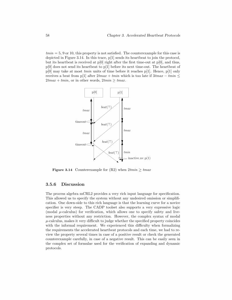
58 Chapter 3. Accelerated Heartbeat Protocols
tmin = 5, 9 or 10, this property is not satisfied. The counterexample for this case isdepicted in Figure 3.14. In this trace, p[1] sends its heartbeat to join the protocol,but its heartbeat is received at p[0] right after the first time-out at p[0], and thus,p[0] does not send its heartbeat to p[1] before its next time-out. The heartbeat ofp[0] may take at most tmin units of time before it reaches p[1]. Hence, p[1] onlyreceives a beat from p[1] after 2tmax + tmin which is too late if 3tmax − tmin ≤2tmax + tmin, or in other words, 2tmin ≥ tmax .
p[0]
timeout
p[1]
tmax
tmax
beat(>)
timeout
inactive nv p(1)
tmax
tminbeat(>)
tmax
beat(>)
beat(>)
Figure 3.14 Counterexample for (R2) when 2tmin ≥ tmax
3.5.6 Discussion
The process algebra mCRL2 provides a very rich input language for specification.This allowed us to specify the system without any undesired omission or simplifi-cation. One down-side to this rich language is that the learning curve for a novicespecifier is very steep. The CADP toolset also supports a very expressive logic(modal µ-calculus) for verification, which allows one to specify safety and live-ness properties without any restriction. However, the complex syntax of modalµ-calculus, makes it very difficult to judge whether the specified property coincideswith the informal requirement. We experienced this difficulty when formalizingthe requirements the accelerated heartbeat protocols and each time, we had to re-view the property several times in case of a positive result or check the generatedcounterexample carefully, in case of a negative result. This can be easily seen inthe complex set of formulae used for the verification of expanding and dynamicprotocols.
3.6 Correcting the protocols 59
On the other hand, UPPAAL provides a graphical input language which is very,easy to learn and use. A clear advantage of UPPAAL’s specification language fortimed systems is its built-in timed constructs such as clocks, urgent transitions andurgent and committed states, which make timing specification very concise andreadable. The input language is, however, more restrictive than mCRL2 in thatthe only available data types are the built-in finite data types such as boundedintegers, booleans, records and arrays. Our UPPAAL models are in that sensemore static than mCRL2 models, e.g., the number of involved processes is fixedand all the initializations are done statically while in mCRL2 we used lists ofdynamic sizes which can be easily adapted for different instances of the protocol.Another shortcoming of the input language of UPPAAL is its flat compositionof timed-automata. Due to the presence of recursion in mCRL2, one can buildhierarchies of process, which is not possible in UPPAAL. This turned out to beless severe a restriction in our experience since the logic of the processes in eachprotocol can be concisely expressed in one process (an automaton) and nestedprocesses were not necessary to divide and simplify the behavior. As for theproperty specification language, we had to rephrase some of the requirements anduse monitor automata to turn them into reachability properties. This is in generala non-trivial task and may involve simplification of the requirements, however,we could make a faithful translation of our requirements into a combination ofmonitor automata and reachability properties. This is mainly due to the fact thatour requirements did not involve many (nested) fixed point constructs.
Concerning the verification possibilities, overall, we got much faster results fromUPPAAL. For the expanding and dynamic protocols, the verification time of eachproperty was in the order of ten minutes to half an hour using UPPAAL 4.0 whilethe same properties took a few hours to be verified by the mCRL2 toolset. This canbe attributed due to dedicated algorithms for analyzing time-related properties inUPPAAL; this is consistent with earlier observations, e.g., communicated by theauthors of [37], that mCRL2 (or its precursor muCRL) can provide faster resultsif the correctness properties do not involve timing, but currently, UPPAAL out-performs mCRL2 when timing is relevant in the correctness requirements (whichis the case for our case-study).
3.6 Correcting the protocols
As observed in Section 3.5.5, all requirements of the protocols are violated undercertain circumstances. These violations can be traced back to two main causes:inappropriate handling of simultaneous events and incorrect time-bounds for theinactivation of processes. In the remainder of this section, we explain the natureof these causes and propose fixes that can fix the discovered problems and evenimprove the performance of accelerated heartbeat protocols.
60 Chapter 3. Accelerated Heartbeat Protocols
3.6.1 Simultaneous events
One clear source of problem in all heartbeat protocols is the possibility of simulta-neous events and lack of appropriate treatment thereof. Particularly, if a heartbeatis received simultaneously with the occurrence of a timeout, the timeout may getprecedence and thus, the receiving process may become non-voluntarily inactivewhile the sending process is still alive and in fact has sent its heartbeat on time.This results in a violation of properties R2 and R3 (see Figures 3.12 and 3.13).To solve this problem, receive operations must be given precedence over timeouts,i.e., before processing timeouts, it has to be checked whether the communicationchannels offer messages that have to be delivered or not. In the former case, thepending messages are first processed and then timeouts are issued.
Adopting the priorities specified above removes all the counterexamples reportedfor R2 and R3 for binary and static heartbeat protocols. This fix is essential forsolving the problems regarding the same properties for the expanding and dynamicprotocols, but it is not sufficient as explained below.
3.6.2 Incorrect time-bounds
All heartbeat protocols assume a total waiting time of 2tmax for p[0] and 3tmax −tmin for p[i] process(es), respectively. We argue below that both of the above-mentioned time-bounds are either incorrect or imprecise (depending on the typeof the protocol). Incorrectness of time-bounds leads to violation of properties R1and R2 and imprecision leads to inefficiency of the protocol (i.e., unnecessarilylong delays before detecting a process or channel failure).
Time bounds for the binary and static heartbeat protocols
As for the total waiting time for p[0], the maximum time between between re-ceiving the last heartbeat from p[1] to the non-voluntary inactivation of p[0] isachieved when p[1] crashes at the beginning of the first round right after sendingits heartbeat to p[0]. To maximize the total waiting time, assume that the heart-beat of p[1] is received at p[0] instantaneously. We distinguish the following twocases:
• 2tmin > tmax : In this case, the maximal waiting time of p[0] is indeed 2tmaxsince after the second round, the waiting time is reduced to tmax/2 and sinceit holds that tmax/2 < tmin, p[0] will be non-voluntarily inactivated.
• 2tmin ≤ tmax : In this case, the maximal waiting time of p[0] is 3tmax−tminaccording to the calculation given below.
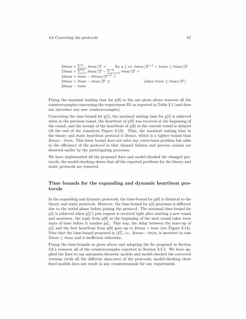
3.6 Correcting the protocols 61
2tmax +∑ji=1 tmax/2i = for a j s.t. tmax/2j+1 < tmin ≤ tmax/2j
2tmax +∑∞i=1 tmax/2i −∑∞
i=j+1 tmax/2i =
2tmax + tmax − 2tmax/2j+1 =2tmax + tmax − tmax/2j ≤ (since tmin ≤ tmax/2j)3tmax − tmin
Fixing the maximal waiting time for p[0] to the one given above removes all thecounterexamples concerning the requirement R1 as reported in Table 3.1 (and doesnot introduce any new counterexamples).
Concerning the time bound for p[1], the maximal waiting time for p[1] is achievedwhen in the previous round, the heartbeat of p[0] was received at the beginning ofthe round, and the receipt of the heartbeat of p[0] in the current round is delayedtill the end of the round(see Figure 3.13). Thus, the maximal waiting time inthe binary and static heartbeat protocol is 2tmax, which is a tighter bound than3tmax− tmin. This lower bound does not solve any correctness problem but addsto the efficiency of the protocol in that channel failures and process crashes aredetected earlier by the participating processes.
We have implemented all the proposed fixes and model-checked the changed pro-tocols; the model-checking shows that all the reported problems for the binary andstatic protocols are removed.
Time bounds for the expanding and dynamic heartbeat pro-tocols
In the expanding and dynamic protocols, the time-bound for p[0] is identical to thebinary and static protocols. However, the time-bound for p[i] processes is differentdue to the initial phase before joining the protocol. The maximal time-bound forp[i] is achieved when p[i]’s join request is received right after starting a new roundand moreover, the reply from p[0] at the beginning of the next round takes tminunits of time before it reaches p[i]. This way, the delay between the start-up ofp[i] and the first heartbeat from p[0] goes up to 2tmax + tmin (see Figure 3.14).Note that the time-bound proposed in [47], i.e., 3tmax− tmin, is incorrect in case2tmin ≥ tmax and is inefficient otherwise.
Fixing the time-bounds as given above and adopting the fix proposed in Section3.6.1 removes all of the counterexamples reported in Section 3.5.5. We have ap-plied the fixes to our automata-theoretic models and model-checked the correctedversions (with all the different data-sets) of the protocols; model-checking thesefixed models does not result in any counterexample for any requirement.
62 Chapter 3. Accelerated Heartbeat Protocols
3.7 Conclusions
We formalized different versions of heartbeat protocols as specified in [47, 78] inthe process algebra mCRL2 and timed-automata-theoretic formalism of UPPAAL.We then formalized some natural properties on these protocols and verified themusing the CADP tool-set and UPPAAL. We reported several counterexamplesthat were discovered during our formal analysis. The properties that are notsatisfied by the accelerated heartbeat protocols are quite natural and essential.Hence, we proposed subsequent improvements on the protocols in order to meetthese requirements. We model-checked the improved versions of the protocols andshowed that they indeed satisfy our requirements.
We believe that the specifications developed in the course of researching heartbeatprotocols can be readily used to verify similar protocols and protocols that buildupon them, e.g., protocols for failure detectors. We have followed this line andapplied our method to verify the correctness of failure detector protocols, see, e,g.,Chapter 6. Moreover, in the present version of the dynamic heartbeat protocol, anupper bound on the number of processes should be a priori known and additionally,a process can never join the protocol once it has left it. An improved version ofthe dynamic heartbeat protocol allowing for an unbounded number of processes,which can join and leave at any time and proving the correctness of the extendedprotocol is also a future research goal.
Chapter 4
Formal Analysis ofConsensus Protocols inAsynchronous DistributedSystems
Formal Analysis of Consensus Protocols in Asynchronous Distributed Systems. CS-Report09-16, Eindhoven University of Technology, 2009.
64 Chapter 4. Consensus Protocols in Asynchronous Distributed Systems
4.1 Introduction
This chapter presents a formal verification of two consensus protocols for dis-tributed systems presented in [22]. These two protocols rely on two underlyingfailure detection protocols. We formalize an abstract model of the underlyingfailure detection protocols and building upon this abstract model, formalize thetwo consensus protocols. We prove that both algorithms satisfy the properties of“uniform agreement”, “uniform integrity”, “termination” and “uniform validity”assuming the correctness of their corresponding failure detectors.
In a consensus protocol, each participating process proposes a value and eventuallyall (non-crashed) processes should reach a state in which they decide upon the samevalue. The decided value has to be chosen from the set of proposed values by theparticipating processes [39]. In an asynchronous environment, there is no upperbound on the delay of (reliable) communication channels; hence, a process cannotdistinguish between a crashed process, for whose proposed value it does not haveto wait, and a process connected to a very slow communication channel, whoseproposed value has to be taken into account in the final result of the consensus.This forms the basic argument behind the impossibility of solving the consensusproblem in an asynchronous environment in the presence of crash failures [40].
To circumvent this problem, the consensus protocols are built upon failure de-tectors, which by a synchronization mechanism can provide us with informationabout crashed (i.e., permanently halted) and correct processes. Upon query at anygiven time, the failure detector of each process outputs the list of its suspectedprocesses. The information provided by a failure detector is not necessarily accu-rate and hence, failure detectors can only suspect other processes. The unreliablefailure detectors are in turn the result of unbounded delays in the asynchronouscommunication channels. Hence, at each moment of time, the output of any twofailure detectors can be different.
We formalize and verify two algorithms (also called protocols) for solving the con-sensus problem proposed by [22]; one uses strong completeness with weak accuracyand the other uses strong completeness with eventual weak accuracy. Strong com-pleteness refers to suspecting all crashed processes, i.e., after a certain amountof time every correct process permanently suspects each crashed process. Weakaccuracy means that some correct process is never suspected. Eventual weak ac-curacy means that after a certain amount of time, some correct process is neversuspected. The first consensus protocol, relying on strongly complete and weaklyaccurate failure detectors, tolerates N − 1 number of process-failures (N is the to-tal number of processes in asynchronous systems) whereas the second one, relyingon a strongly complete and eventually weakly accurate failure detector, requiresa majority of processes to be correct [22]. If the network guarantees the saidnumber of processes to be correct, we prove that both consensus algorithms sat-isfy functional requirements of uniform agreement, uniform integrity, termination
4.2 Consensus Protocols 65
and uniform validity, to be defined precisely in the remainder of this chapter. Anextended version of this chapter is presented in [11].
Related work. In [43], the consensus algorithm of [22] for eventually weaklyaccurate failure detectors (the second algorithm mentioned above) is formally an-alyzed. The formalization is achieved by providing an operational semantics forthe algorithm in terms of a global transition system (with the configuration rep-resenting message histories and the state of the processes). Then, the authors of[43] provide an inductive proof of correctness for the algorithm. A similar ap-proach has been taken in [81] to prove the properties of the same algorithm usingan intermediate formalism, which is a CCS-like process algebra. The approachof [43, 81] is based on inductive proofs, which require human intervention. How-ever, our approach is based on model-checking and the verification procedure isfully mechanized. A major hurdle in applying model checking to the second con-sensus algorithms is the unbounded nature of round numbers (and consequentlyother data structures such as time-stamps). We overcome this problem by divid-ing our verification problem into two sub-problems, namely before and after thatthe failure detector has reached its weakly accurate phase. We apply boundedmodel-checking to the first sub-problem and exhaustively model-check the secondone.
In [96], model checking has been applied to consensus algorithms of [25] and [26],where the latter is a variant of the renown Paxos algorithm of [68]. The maincrux of the approach of [96] is to use an abstraction of the process and channelstates using the Hear-Of (HO) model of [27]. In [97] the approach of [96] has beenimproved by dividing the proof obligation into a few proof obligations to whichbounded model-checking can be applied. This approach bears some resemblanceto our approach in applying bounded model-checking to the second algorithm.However, the HO model is not directly applicable to our setting, as observed in[24], due to the intrinsically strong assumptions of failure detectors. Applyingvariants of Heard-Of model to our setting is the subject of our ongoing research.
Structure of the chapter. We give an informal description of the two consensusprotocols in Sections 4.2.2 and 4.2.3 and process-algebraic specifications of themin Sections 4.3.2 and 4.3.3, respectively. The requirements of the protocols andthe results of our formal analyses are presented in Section 4.4. The chapter isconcluded in Section 4.5.
4.2 Consensus Protocols
Consensus protocols ensure that all correct processes eventually reach a unanimousagreement on one value, called the decided value. The decided value is always
66 Chapter 4. Consensus Protocols in Asynchronous Distributed Systems
selected from a set of values, to which every process (at the beginning of theprotocol) contributes one value, called the proposed value, to this set. The processwill not come to a decision if it crash fails before reaching a decision. A failurepattern, denoted by F in the remaining text, is a function from T to 2π, where Tis the set of natural numbers, denoting discrete time, and π = {p1, p2, . . . , pn} isthe set of participating processes. During the execution of the protocols, a failuredetector D makes (possibly unreliable) information available about the failurepattern F . Next we explain the general assumptions on which the forthcomingalgorithms rely.
4.2.1 General assumptions
1. If a process is crashed, it will never recover. Assume that F (t) denotes theset of crashed processes up to time t then F (t) ⊆ F (t+ 1).
2. All failure detectors are unreliable. This means that they can suspect correctprocesses or unsuspect crashed processes at any time. Hence, in general foreach process p, H(p, t) is unrelated to H(p, t+1) where H is a function fromπ×T to 2π for failure detector history and it provides the history of a failuredetector Dp up to time t, i.e., a timed trace of lists of processes suspectedby pi up to time t. It is assumed that there is a discrete global clock thatacts as a fictional device and the processes do not have access to it. Due tounreliability of failure detectors, it is also possible for two distinct processesp and q that H(p, t) 6= H(q, t) at some time t.
3. A solution for the consensus problem is proposed in the setting of asyn-chronous distributed systems in which there is no upper bound on:
(a) message delays,
(b) clock drifts, and
(c) the amount of time necessary to execute a step.
4. The failure detectors of all correct process participants satisfy strong com-pleteness, i.e., eventually every crashed process is permanently suspected bytheir failure detectors. Due to [22], the following formula formalizes thisdescription.
∀F, ∀H ∈ D(F ), ∃t ∈ T, ∀p ∈ crashed(F ),
∀q ∈ correct(F ),∀t′ ≥ t : p ∈ H(q, t′)
D(F ) is a set of failure detector histories and correct(F ) = π − crashed(F )where crashed(F ) =
⋃t∈T F (t).
4.2 Consensus Protocols 67
5. Although the failure detectors are unreliable, they are assumed to satisfysome notion of accuracy. A failure detector is weakly accurate when somecorrect process is never suspected; it is eventually weakly accurate, if it even-tually never suspects some correct process. The following formula, due to[22], formalizes this description.
∀F, ∀H ∈ D(F ), ∃p ∈ correct(F ), ∀t ∈ T, ∀q ∈ π − F (t) : p /∈ H(q, t)
The above-given formula formalizes weak accuracy if t is universally quan-tified and formalizes eventual weak accuracy if t is existentially quantifiedover T.
6. The consensus algorithm that relies on strong completeness with weak ac-curacy can tolerate any number of process failures whereas the other con-sensus algorithm requiring strong completeness and eventual weak accuracy,requires the majority of the processes to be correct.
7. The communication channel between each pair of processes is reliable.
Along with the property of strong completeness, the algorithms discussed in Sec-tions 4.2.2 and 4.2.3 rely on the above assumptions together with the propertiesof weak accuracy and eventual weak accuracy, respectively.
4.2.2 Solving consensus using strong completeness and weakaccuracy
This algorithm assumes the properties of strong completeness and weak accuracyand solves the consensus problem in an asynchronous system provided that at leastone correct process is never suspected by any failure detector. The algorithm hasthree phases and each process, if it remains operational, is supposed to go throughall phases (from the first to the last). Suppose that n is the total number ofprocesses in the network. In the first phase, each (non-crashed) process p executesn − 1 rounds. In every round each process broadcasts a message that containsits proposed value vp and then receives the same type of message from otherunsuspected processes. At the end of this phase, every process updates its set ofproposed values. These values are obtained either directly from other processes orindirectly in that some processes are still alive but erroneously suspected.
In the second phase, all participating (non-crashed) processes exchange their setsof values and make them identical to each other by dropping the values that arenot part of some received set. In the third and last phase, each process decides thefirst available value in its set. The algorithm for solving the consensus problemusing strong completeness and weak accuracy, due to [22], is given below such thatevery process p executes it with a distinct proposed value vp.
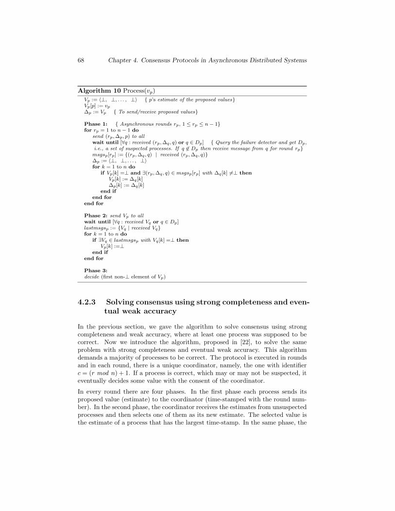
68 Chapter 4. Consensus Protocols in Asynchronous Distributed Systems
Algorithm 10 Process(vp)
Vp := 〈⊥, ⊥, . . . , ⊥〉 { p’s estimate of the proposed values}Vp[p] := vp∆p := Vp { To send/receive proposed values}
Phase 1: { Asynchronous rounds rp, 1 ≤ rp ≤ n− 1}for rp = 1 to n− 1 do
send (rp,∆p, p) to allwait until [∀q : received (rp,∆q , q) or q ∈ Dp] { Query the failure detector and get Dp,i.e., a set of suspected processes. If q 6∈ Dp then receive message from q for round rp}msgsp[rp] := {(rp,∆q , q) | received (rp,∆q , q)}∆p := 〈⊥, ⊥, . . . , ⊥〉for k = 1 to n do
if Vp[k] =⊥ and ∃(rp,∆q , q) ∈ msgsp[rp] with ∆q [k] 6=⊥ thenVp[k] := ∆q [k]∆p[k] := ∆q [k]
end ifend for
end for
Phase 2: send Vp to allwait until [∀q : received Vq or q ∈ Dp]lastmsgsp := {Vq | received Vq}for k = 1 to n do
if ∃Vq ∈ lastmsgsp with Vq [k] =⊥ thenVp[k] :=⊥
end ifend for
Phase 3:decide (first non-⊥ element of Vp)
4.2.3 Solving consensus using strong completeness and even-tual weak accuracy
In the previous section, we gave the algorithm to solve consensus using strongcompleteness and weak accuracy, where at least one process was supposed to becorrect. Now we introduce the algorithm, proposed in [22], to solve the sameproblem with strong completeness and eventual weak accuracy. This algorithmdemands a majority of processes to be correct. The protocol is executed in roundsand in each round, there is a unique coordinator, namely, the one with identifierc = (r mod n) + 1. If a process is correct, which may or may not be suspected, iteventually decides some value with the consent of the coordinator.
In every round there are four phases. In the first phase each process sends itsproposed value (estimate) to the coordinator (time-stamped with the round num-ber). In the second phase, the coordinator receives the estimates from unsuspectedprocesses and then selects one of them as its new estimate. The selected value isthe estimate of a process that has the largest time-stamp. In the same phase, the
4.2 Consensus Protocols 69
coordinator broadcasts its estimate. In the third phase, processes receive the valuesent by the coordinator and send back either ack (acknowledgement message) ifthe coordinator is not suspected or otherwise nack (no acknowledgement). In the
fourth phase, the coordinator waits for d (n+1)2 e replies and if at least for d (n+1)
2 ereplies are of type ack, then estimatec is locked, or otherwise it starts a new roundand consequently other processes waiting for a decision also start a new round.The only reason to send a nack message (in Phase 3) is suspecting the coordinator
(by the failure detector). However, if d (n+1)2 e acknowledgements (ack type mes-
sages) are received, then the coordinator decides the locked value and broadcastsit through a channel, called R-broadcast. Every process p in this protocol executesthe following algorithm [22] where the parameter vp denotes the proposed value.
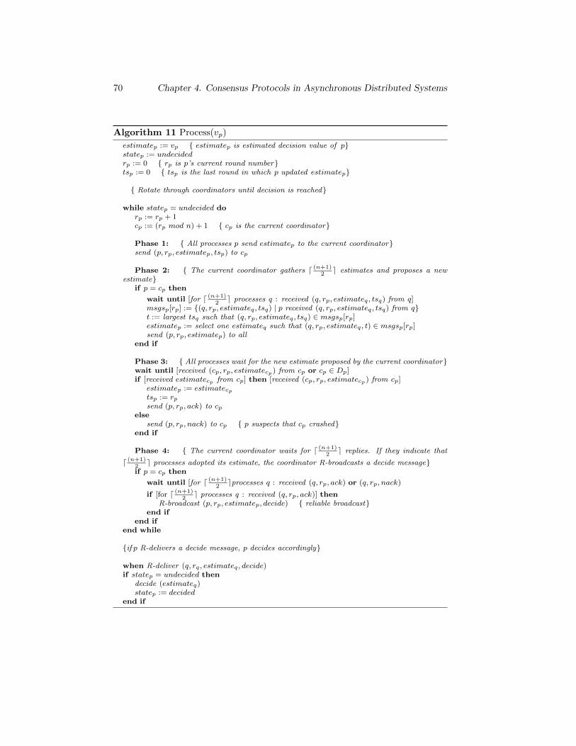
70 Chapter 4. Consensus Protocols in Asynchronous Distributed Systems
Algorithm 11 Process(vp)
estimatep := vp { estimatep is estimated decision value of p}statep := undecidedrp := 0 { rp is p’s current round number}tsp := 0 { tsp is the last round in which p updated estimatep}
{ Rotate through coordinators until decision is reached}
while statep = undecided dorp := rp + 1cp := (rp mod n) + 1 { cp is the current coordinator}
Phase 1: { All processes p send estimatep to the current coordinator}send (p, rp, estimatep, tsp) to cp
Phase 2: { The current coordinator gathers d (n+1)2e estimates and proposes a new
estimate}if p = cp then
wait until [for d (n+1)2e processes q : received (q, rp, estimateq , tsq) from q]
msgsp[rp] := {(q, rp, estimateq , tsq) | p received (q, rp, estimateq , tsq) from q}t := largest tsq such that (q, rp, estimateq , tsq) ∈ msgsp[rp]estimatep := select one estimateq such that (q, rp, estimateq , t) ∈ msgsp[rp]send (p, rp, estimatep) to all
end if
Phase 3: { All processes wait for the new estimate proposed by the current coordinator}wait until [received (cp, rp, estimatecp ) from cp or cp ∈ Dp]if [received estimatecp from cp] then [received (cp, rp, estimatecp ) from cp]
estimatep := estimatecptsp := rpsend (p, rp, ack) to cp
elsesend (p, rp, nack) to cp { p suspects that cp crashed}
end if
Phase 4: { The current coordinator waits for d (n+1)2e replies. If they indicate that
d (n+1)2e processes adopted its estimate, the coordinator R-broadcasts a decide message}
if p = cp then
wait until [for d (n+1)2eprocesses q : received (q, rp, ack) or (q, rp, nack)
if [for d (n+1)2e processes q : received (q, rp, ack)] then
R-broadcast (p, rp, estimatep, decide) { reliable broadcast}end if
end ifend while
{if p R-delivers a decide message, p decides accordingly}
when R-deliver (q, rq , estimateq , decide)if statep = undecided then
decide (estimateq)statep := decided
end if
4.3 Formal Specification 71
4.3 Formal Specification
In this section, we discuss the formalization of the consensus Algorithms 10 and10, given in Sections 4.2.2 and 4.2.3, respectively. We use mCRL2 [50] as ourformal specification language. We need some data types, functions and operatorsto specify the behaviour of the protocols in terms of communication channels,failure detectors and the different phases of the protocols. We face the followingchallenges while formally specifying these protocols.
• To fully realize asynchrony in the underlined distributed system, we haveto use separate channel for every type of message in every round at everyphase. Due to this scheme, it is guaranteed that there is no bound on messagedelays and a message sent in a previous round can reach its destination aftera message of the current round.
• In the second algorithm, the number of rounds till reaching consensus ispotentially unbounded and this poses a serious challenge in model checkingthe algorithm.
We overcome this challenge by dividing the verification of the second algo-rithm into two parts: first, we apply bounded model-checking on the proper-ties of the algorithm that are to be satisfied before the weakly accurate phaseof the failure detector and secondly, we apply exhaustive model-checking onall properties after that the failure detector has become weakly accurate.
• Failure detectors are abstract entities without a specific implementation; alsotheir communication media with processes are unspecified. This leaves someroom for design decisions in the formal model. For example in the first twophases of Algorithm 10 and Phase 3 of Algorithm 11, it is mentioned that aprocess either receives a message from an arbitrary process q or suspects it(i.e., q ∈ Dp). In the formal model, this can be specified as a nondetermin-istic choice between receiving a message and querying the failure detector.However, this naive implementation leads to a diverging behaviour in query-ing the failure detector even there is some value available to receive. Weavoid this by updating the failure detector information once in a round andallowing the failure detector to push its updates, if any, through the roundrather than polling the information each time.
• In the second algorithm, there is a parallel process which takes care of re-ceiving decisions and deciding upon them. However, there is insufficient in-formation about the communication between the participating process andthe deciding process, which is necessary to guarantee termination when itrealizes consensus.
We discuss our approach to address these issues in the remainder of this chapter.
72 Chapter 4. Consensus Protocols in Asynchronous Distributed Systems
4.3.1 Data types
We use the built-in support for standard data types in mCRL2 such as Booleansand natural numbers. We use lists to handle arrays of homogeneous data, e.g.,estimates, msgs, and lastMsgs.
4.3.2 Consensus with strong completeness and weak accu-racy
Before discussing the formalization details of the protocol, we present the auxiliaryfunctions, which are defined in the form of rewrite rules. Function types are usedto define customized transformations on (a combination of) abstract data types.
• minus: To subtract a list from another, e.g., if A and B are two lists ofnatural numbers then minus(A,B) is also a list having all such elements ofA which do not belong to B. This definition is formally specified as:
mapminus : List(N)× List(N)→ List(N);eliminate : List(N)× N→ List(N);{to eliminate the first occurrence of a value from the list}
varln, lg : List(N);m,n : N;
eqnminus([], lg) = []; {[] is an empty list}minus(ln, []) = ln;minus(n� ln,m� lg) =if(m ∈ n� ln,minus(eliminate(n� ln,m), lg),minus(n� ln, lg));{� is the operator to insert an element at the head of a list}
eliminate(n� ln,m) = if(n ≈ m, ln, n� eliminate(ln,m));
• makeIdentical: This function makes two lists (of the same size) identical byreplacing every element that appears in one but not in the other with ⊥(used for null value) at each location. In Phase 2, processes exchange theirlists of values and using this function make them identical.
4.3 Formal Specification 73
mapmakeIdentical : List(N)× List(N)→ List(N);varln : List(N);x, n : N;eqnmakeIdentical([], ln) = ln;makeIdentical(ln, []) = [];makeIdentical(x� lg, n� ln) =if(x ≈⊥,⊥ �makeIdentical(lg, ln), n� makeIdentical(lg, ln));
• findDecided: This function finds the first available non-⊥ value from a list.Each process uses this function in Phase 3 to decide a value.
mapfindDecided : List(N)→ N;varln : List(N);n : N;eqnfindDecided([]) =⊥;findDecided(n� ln) = if(n 6≈⊥, n,findDecided(ln));
• updateDelta: ∆ is the list used in every round of Phase 1 to send the proposedvalue to all other processes. After sending ∆, each process initializes it with⊥ and then updates it with the values received in the current round but notin the previous rounds. To update the data values in this list, the functionupdateDelta is used. This function is only defined when the three lists havethe same size.
mapupdateDelta : List(N)× List(N)× List(N)→ List(N);varlg, ln, ld : List(N);x, n,m : N;eqnupdateDelta([], lg, ln) = [];updateDelta(n� lg,m� ln, x� ld) =if(m 6≈ n,m� updateDelta(lg, ln, ld), x� updateDelta(lg, ln, ld));
• updateMsgs: In phases 1 and 2 processes use two lists msgs and lastmsgsrespectively to store the messages from other participating processes. Thefollowing function is used to store a list at a particular location.
74 Chapter 4. Consensus Protocols in Asynchronous Distributed Systems
mapupdateMsgs : N× List(List(N))× List(N)→ List(List(N))varlg, ln : List(N);n : N;msgs : List(List(N));eqnupdateMsgs(⊥, lg �msgs, ln) = ln�msgs;updateMsgs(⊥, [], ln) = [ln];(n > 0)→ updateMsgs(n, lg �msgs, ln) =lg � updateMsgs(Int2Nat(n− 1),msgs, ln);{Int2Nat function determines the natural number of an integer value}
• updateBoolList : To replace a value at specific location with a given B typevalue in a list of Booleans.
mapupdateBoolList : List(B)× N× B→ List(B);varlb : List(B);n : N;s, b : BeqnupdateBoolList(s� lb, n, b) =
if(n ≈ 0, b� lb, s� updateBoolList(lb, Int2Nat(n− 1), b));
• updateLastMsgs: In Phase 2, every process uses the list lastmsgs to store thelist V received from other processes. After receiving all messages, a processp updates Vp with respect to each entry of lastmsgs. We use this function toupdate Vp of a process p.
mapupdateLastMsgs : List(List(N))× List(N)× B→ List(B);varln, lg : List(N);msgs : List(List(N));eqnupdateLastMsgs([], ln) = ln;updateLastMsgs(lg �msgs, ln) =
if(#msgs > 0, updateLastMsgs(msgs,makeIdentical(lg, ln)),makeIdentical(lg, ln));
Next we discuss the process definitions which specify the behaviour of every par-ticipant in the protocol.
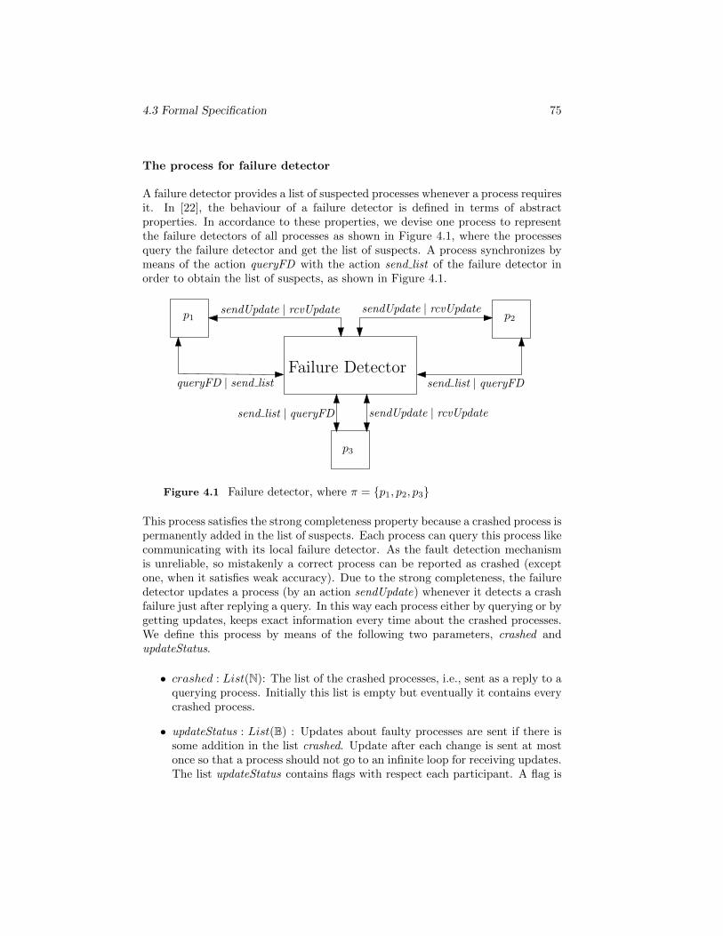
4.3 Formal Specification 75
The process for failure detector
A failure detector provides a list of suspected processes whenever a process requiresit. In [22], the behaviour of a failure detector is defined in terms of abstractproperties. In accordance to these properties, we devise one process to representthe failure detectors of all processes as shown in Figure 4.1, where the processesquery the failure detector and get the list of suspects. A process synchronizes bymeans of the action queryFD with the action send list of the failure detector inorder to obtain the list of suspects, as shown in Figure 4.1.
p1 p2
p3
Failure Detector
sendUpdate | rcvUpdate
sendUpdate | rcvUpdatesendUpdate | rcvUpdate
send list | queryFD
send list | queryFD
queryFD | send list
Figure 4.1 Failure detector, where π = {p1, p2, p3}
This process satisfies the strong completeness property because a crashed process ispermanently added in the list of suspects. Each process can query this process likecommunicating with its local failure detector. As the fault detection mechanismis unreliable, so mistakenly a correct process can be reported as crashed (exceptone, when it satisfies weak accuracy). Due to the strong completeness, the failuredetector updates a process (by an action sendUpdate) whenever it detects a crashfailure just after replying a query. In this way each process either by querying or bygetting updates, keeps exact information every time about the crashed processes.We define this process by means of the following two parameters, crashed andupdateStatus.
• crashed : List(N): The list of the crashed processes, i.e., sent as a reply to aquerying process. Initially this list is empty but eventually it contains everycrashed process.
• updateStatus : List(B) : Updates about faulty processes are sent if there issome addition in the list crashed. Update after each change is sent at mostonce so that a process should not go to an infinite loop for receiving updates.The list updateStatus contains flags with respect each participant. A flag is
76 Chapter 4. Consensus Protocols in Asynchronous Distributed Systems
true if a fault is detected and is toggled if the respective update is sent orthe respective query is replied.
1: FD(crashed : List(N), updateStatus : List(B)) =
2:∑id:N
rcvCrashed(id) · FD(id� crashed, [true,true,true])
3: +4:
∑n:N
(
5: send list(crashed, n)6: +7: (0 ∈ minus(PI, crashed) ∧ n 6= 0)→ send list(0 � crashed, n)8: +9: (1 ∈ minus(PI, crashed) ∧ n 6= 1)→ send list(1 � crashed, n)
10: +11: (#crashed ≈ 0 ∧ n ≈ Correct)→ send list(0 � 1 � crashed, n)12: +13: (updateStatus · n)→14: ( sendUpdate(crashed, n)15: +16: (0 ∈ minus(PI, crashed) ∧ n 6= 0)→ sendUpdate(0 � crashed, n)17: +18: (1 ∈ minus(PI, crashed) ∧ n 6= 1)→ sendUpdate(1 � crashed, n)19: +20: (#crashed ≈ 0 ∧ n ≈ Correct)→ sendUpdate(0 � 1 � crashed, n)21: )22: ) · FD(crashed, updateBoolList(updateStatus, n, false));
The name of the process for the failure detector is FD as shown in line 1 withtwo parameter, crashed and updateStatus. Line 2 shows detecting a crash failureand then adding id of that crashed process to the list crashed. This line alsoshows making the updateStatus of all three processes true which indicates sendingupdates later on. Upon replying a query or sending an update, updateStatus of thecommunicating process becomes false (line 22). Line 5 shows sending the crashedlist to an arbitrary process n. Without loss of generality, we assume that process2 is the correct proces, i.e., it never crashes. So, lines 7 and 9, respectively showadding processes 0 and 1 to suspects when they are not detected as crashed. Line11 shows that if the correct process queries and the crashed list is empty thenboth the processes 0 and 1 can be reported as crashed. This is the scheme we useto model unreliability of the failure detector and the property of weak accuracy.Because the failure detector satisfies the property of strong completeness, so everycrash failure is reported as crashed. Lines from 14 to 20 are similar to lines from 5
4.3 Formal Specification 77
to 11 except they are used to send updates from the failure detector. This is whythese lines are guarded by updateStatus and after replying, the respective flag istoggled (line 22).
The process for Phase 1:
At this phase a process can crash or send its ∆ to others. After sending, a processwaits until ∆ of other participants is received or they are reported as crashed bythe failure detector. We define this process using following six parameters:
• myId :N: The identifier of the process.
• round :N: The round number.
• V : List(N): The list of the proposed values from all unsuspected processes.
• ∆ : List(N): The list to exchange the proposed values, as discussed in Section4.3.2.
• msgs : List(List(N)): The two-dimensional list of the messages from eachprocess in each round.
• msg sent : B: The boolean flag indicating whether the first message of theround has been sent out or not.
In the following definition we assume the existence of a process Correct that re-mains operational and never gets suspected where Correct ∈ π.
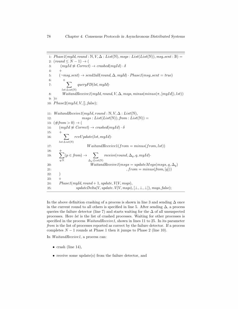
78 Chapter 4. Consensus Protocols in Asynchronous Distributed Systems
1: Phase1(myId, round : N, V,∆ : List(N),msgs : List(List(N)),msg sent : B) =2: (round ≤ N − 1)→ (3: (myId 6≈ Correct)→ crashed(myId) · δ4: +5: (¬msg sent)→ send2all(round,∆,myId) · Phase1(msg sent = true)6: �7:
∑lst:List(N)
queryFD(lst,myId)·
8: WaitandReceive1(myId, round, V,∆,msgs,minus(minus(π, [myId]), lst))9: )�
10: Phase2(myId, V, [], false);
11: WaitandReceive1(myId, round : N, V,∆ : List(N),12: msgs : List(List(N)), from : List(N)) =13: (#from > 0)→ (14: (myId 6≈ Correct)→ crashed(myId) · δ15: +16:
∑lst:List(N)
rcvUpdate(lst,myId)·
17: WaitandReceive1(from = minus(from, lst))18: +19:
∑q:N
(p ∈ from)→∑
∆q :List(N)
receive(round,∆q, q,myId)·
20: WaitandReceive1(msgs = updateMsgs(msgs, q,∆q)21: , from = minus(from, [q]))22: )23: �24: Phase1(myId, round + 1, update V(V,msgs),25: updateDelta(V, update V(V,msgs), [⊥,⊥,⊥]),msgs, false);
In the above definition crashing of a process is shown in line 3 and sending ∆ oncein the current round to all others is specified in line 5. After sending ∆, a processqueries the failure detector (line 7) and starts waiting for the ∆ of all unsuspectedprocesses. Here lst is the list of crashed processes. Waiting for other processes isspecified in the process WaitandReceive1, shown in lines 11 to 25. In its parameterfrom is the list of processes reported as correct by the failure detector. If a processcompletes N − 1 rounds at Phase 1 then it jumps to Phase 2 (line 10).
In WaitandReceive1, a process can:
• crash (line 14),
• receive some update(s) from the failure detector, and
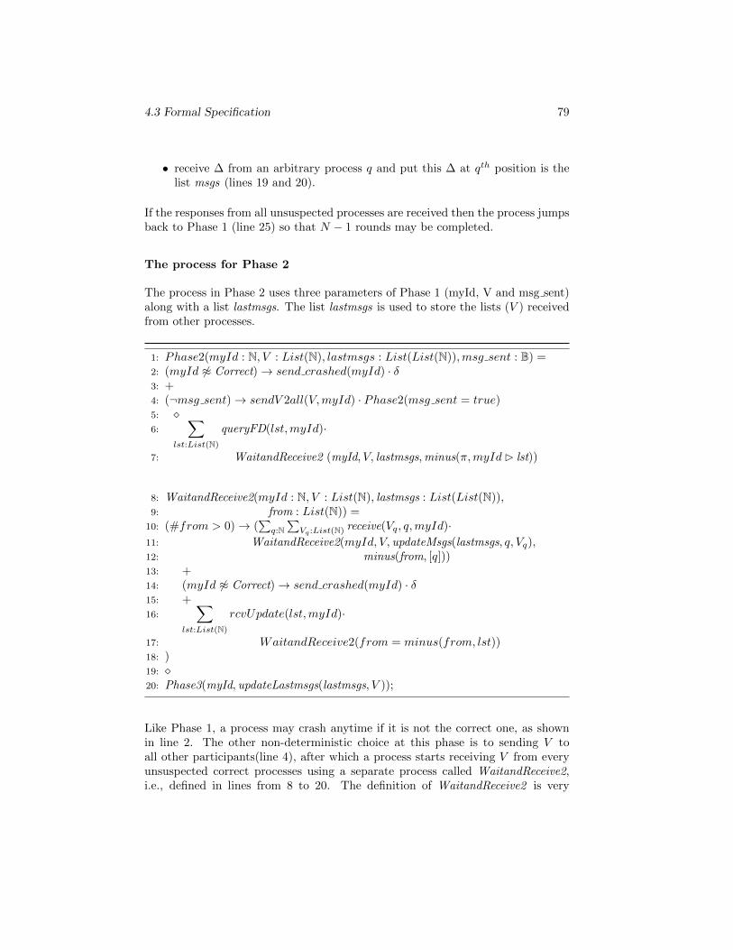
4.3 Formal Specification 79
• receive ∆ from an arbitrary process q and put this ∆ at qth position is thelist msgs (lines 19 and 20).
If the responses from all unsuspected processes are received then the process jumpsback to Phase 1 (line 25) so that N − 1 rounds may be completed.
The process for Phase 2
The process in Phase 2 uses three parameters of Phase 1 (myId, V and msg sent)along with a list lastmsgs. The list lastmsgs is used to store the lists (V ) receivedfrom other processes.
1: Phase2(myId : N, V : List(N), lastmsgs : List(List(N)),msg sent : B) =2: (myId 6≈ Correct)→ send crashed(myId) · δ3: +4: (¬msg sent)→ sendV 2all(V,myId) · Phase2(msg sent = true)5: �6:
∑lst:List(N)
queryFD(lst,myId)·
7: WaitandReceive2 (myId, V, lastmsgs,minus(π,myId� lst))
8: WaitandReceive2(myId : N, V : List(N), lastmsgs : List(List(N)),9: from : List(N)) =
10: (#from > 0)→ (∑q:N
∑Vq :List(N) receive(Vq, q,myId)·
11: WaitandReceive2(myId, V, updateMsgs(lastmsgs, q, Vq),12: minus(from, [q]))13: +14: (myId 6≈ Correct)→ send crashed(myId) · δ15: +16:
∑lst:List(N)
rcvUpdate(lst,myId)·
17: WaitandReceive2(from = minus(from, lst))18: )19: �20: Phase3(myId, updateLastmsgs(lastmsgs, V ));
Like Phase 1, a process may crash anytime if it is not the correct one, as shownin line 2. The other non-deterministic choice at this phase is to sending V toall other participants(line 4), after which a process starts receiving V from everyunsuspected correct processes using a separate process called WaitandReceive2,i.e., defined in lines from 8 to 20. The definition of WaitandReceive2 is very
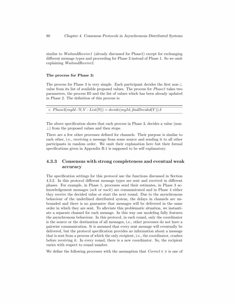
80 Chapter 4. Consensus Protocols in Asynchronous Distributed Systems
similar to WaitandReceive1 (already discussed for Phase1) except for exchangingdifferent message types and proceeding for Phase 3 instead of Phase 1. So we omitexplaining WaitandReceive2.
The process for Phase 3:
The process for Phase 3 is very simple. Each participant decides the first non-⊥value from its list of available proposed values. The process for Phase3 takes twoparameters, the process ID and the list of values which has been already updatedin Phase 2. The definition of this process is:
1: Phase3(myId : N, V : List(N)) = decide(myId,findDecided(V )).δ
The above specification shows that each process in Phase 3, decides a value (non-⊥) from the proposed values and then stops.
There are a few other processes defined for channels. Their purpose is similar toeach other, i.e., receiving a message from some source and sending it to all otherparticipants in random order. We omit their explanation here but their formalspecifications given in Appendix B.1 is supposed to be self explanatory.
4.3.3 Consensus with strong completeness and eventual weakaccuracy
The specification settings for this protocol use the functions discussed in Section4.3.2. In this protocol different message types are sent and received in differentphases. For example, in Phase 1, processes send their estimates, in Phase 3 ac-knowledgement messages (ack or nack) are communicated and in Phase 4 eitherthey receive the decided value or start the next round. Due to the asynchronousbehaviour of the underlined distributed system, the delays in channels are un-bounded and there is no guarantee that messages will be delivered in the sameorder in which they are sent. To alleviate this problematic situation, we instanti-ate a separate channel for each message. In this way our modeling fully featuresthe asynchronous behaviour. In this protocol, in each round, only the coordinatoris the source or the destination of all messages, i.e., other processes do not have apairwise communication. It is assumed that every sent message will eventually bedelivered, but the protocol specification provides no information about a messagethat is sent from a process of which the only recipient, i.e., the coordinator, crashesbefore receiving it. In every round, there is a new coordinator. So, the recipientvaries with respect to round number.
We define the following processes with the assumption that Correct ∈ π is one of
4.3 Formal Specification 81
the correct processes that is never suspected after a certain amount of time.
The process for failure detector
The behaviour of the failure detector shown in this section seems simpler comparedto the one discussed in the Section 4.3.2 because in this algorithm, process areconcerned about the operational status of a coordinator of the current round. Sounreliability of the failure detector is specified only with respect to the coordinator.According to [22], if consensus is not achieved due to the fact that failure detectoris not yet weakly accurate then the participants may continue with unboundedround numbers. Eventually it satisfies weak accuracy, and in such settings thecorrectness of the algorithm is claimed. So, for formal specifications we use thefollowing two schemes with respect to the eventuality of weak accuracy of thefailure detector.
1. The failure detector is initially weakly accurate.
2. The failure detector becomes weakly accurate after some unknown intervalof time.
We discuss our results regarding both of the above mentioned settings in Section4.4.2. In the second version, the failure detector may or may not be weakly accu-rate. Then unboundedness of rounds is a big challenge because we can model suchbehaviour but cannot completely model-check, particularly because sent messagesare time-stamped with round numbers. So, we need some upper bound on roundnumbers and in this chapter we model with N number of rounds where N is thenumber of participant. In this way every participant gets a chance to be the coor-dinator and reach a decision. This remains a bounded search of the state-space,which is infinite and hence cannot be fully covered in its original form.
In this protocol the majority of the processes remains correct and we implementthis property with the help of a failure detector. It keeps track of the number of
crashes (f) and guarantees that f < d (n+1)2 e. In the definition two parameters
crashed and updateStatus are used which we already discussed in the Section 4.3.2.
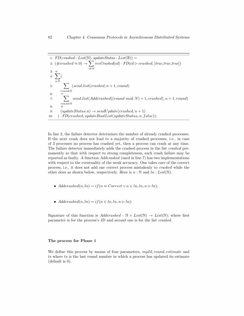
82 Chapter 4. Consensus Protocols in Asynchronous Distributed Systems
1: FD(crashed : List(N), updateStatus : List(B)) =
2: (#crashed ≈ 0)→∑id:N
rcvCrashed(id) · FD(id� crashed, [true,true,true])
3: +4:
∑n:N
(
5:∑
round:N(send list(crashed, n+ 1, round)
6: +7:
∑round:N
send list(Addcrashed((round mod N) + 1, crashed), n+ 1, round)
8: +9: (updateStatus.n)→ sendUpdate(crashed, n+ 1)
10: ) · FD(crashed, updateBoolList(updateStatus, n, false));
In line 2, the failure detector determines the number of already crashed processes.If the next crash does not lead to a majority of crashed processes, i.e., in caseof 3 processes no process has crashed yet, then a process can crash at any time.The failure detector immediately adds the crashed process in the list crashed per-manently so that with respect to strong completeness, each crash failure may bereported as faulty. A function Addcrashed (used in line 7) has two implementationswith respect to the eventuality of the weak accuracy. One takes care of the correctprocess, i.e., it does not add one correct process mistakenly to crashed while theother does as shown below, respectively. Here is n : N and ln : List(N).
• Addcrashed(n, ln) = if(n ≈ Correct ∨ n ∈ ln, ln, n� ln);
• Addcrashed(n, ln) = if(n ∈ ln, ln, n� ln);
Signature of this function is Addcrashed : N × List(N) → List(N); where firstparameter is for the process’s ID and second one is for the list crashed.
The process for Phase 1
We define this process by means of four parameters, myId, round, estimate andts where ts is the last round number in which a process has updated its estimate(default is 0).
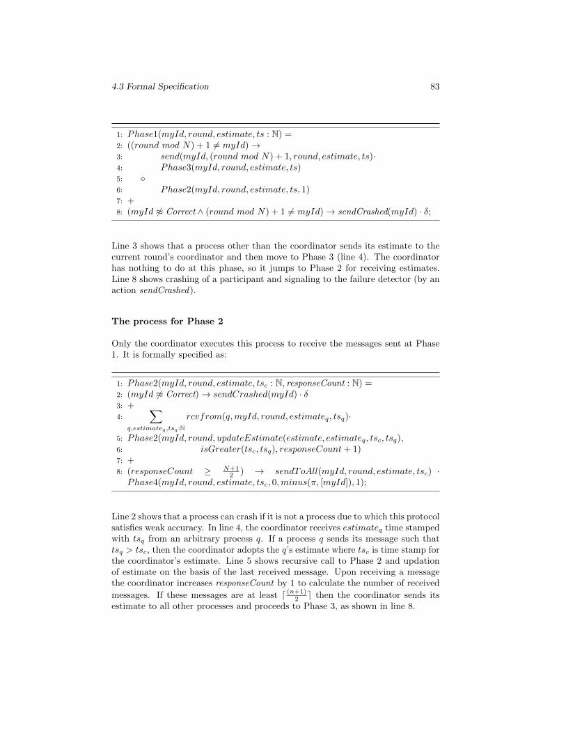
4.3 Formal Specification 83
1: Phase1(myId, round, estimate, ts : N) =2: ((round mod N) + 1 6= myId)→3: send(myId, (round mod N) + 1, round, estimate, ts)·4: Phase3(myId, round, estimate, ts)5: �6: Phase2(myId, round, estimate, ts, 1)7: +8: (myId 6≈ Correct ∧ (round mod N) + 1 6= myId)→ sendCrashed(myId) · δ;
Line 3 shows that a process other than the coordinator sends its estimate to thecurrent round’s coordinator and then move to Phase 3 (line 4). The coordinatorhas nothing to do at this phase, so it jumps to Phase 2 for receiving estimates.Line 8 shows crashing of a participant and signaling to the failure detector (by anaction sendCrashed).
The process for Phase 2
Only the coordinator executes this process to receive the messages sent at Phase1. It is formally specified as:
1: Phase2(myId, round, estimate, tsc : N, responseCount : N) =2: (myId 6≈ Correct)→ sendCrashed(myId) · δ3: +4:
∑q,estimateq,tsq :N
rcvfrom(q,myId, round, estimateq, tsq)·
5: Phase2(myId, round, updateEstimate(estimate, estimateq, tsc, tsq),6: isGreater(tsc, tsq), responseCount+ 1)7: +8: (responseCount ≥ N+1
2 ) → sendToAll(myId, round, estimate, tsc) ·Phase4(myId, round, estimate, tsc, 0,minus(π, [myId]), 1);
Line 2 shows that a process can crash if it is not a process due to which this protocolsatisfies weak accuracy. In line 4, the coordinator receives estimateq time stampedwith tsq from an arbitrary process q. If a process q sends its message such thattsq > tsc, then the coordinator adopts the q’s estimate where tsc is time stamp forthe coordinator’s estimate. Line 5 shows recursive call to Phase 2 and updationof estimate on the basis of the last received message. Upon receiving a messagethe coordinator increases responseCount by 1 to calculate the number of received
messages. If these messages are at least d (n+1)2 e then the coordinator sends its
estimate to all other processes and proceeds to Phase 3, as shown in line 8.
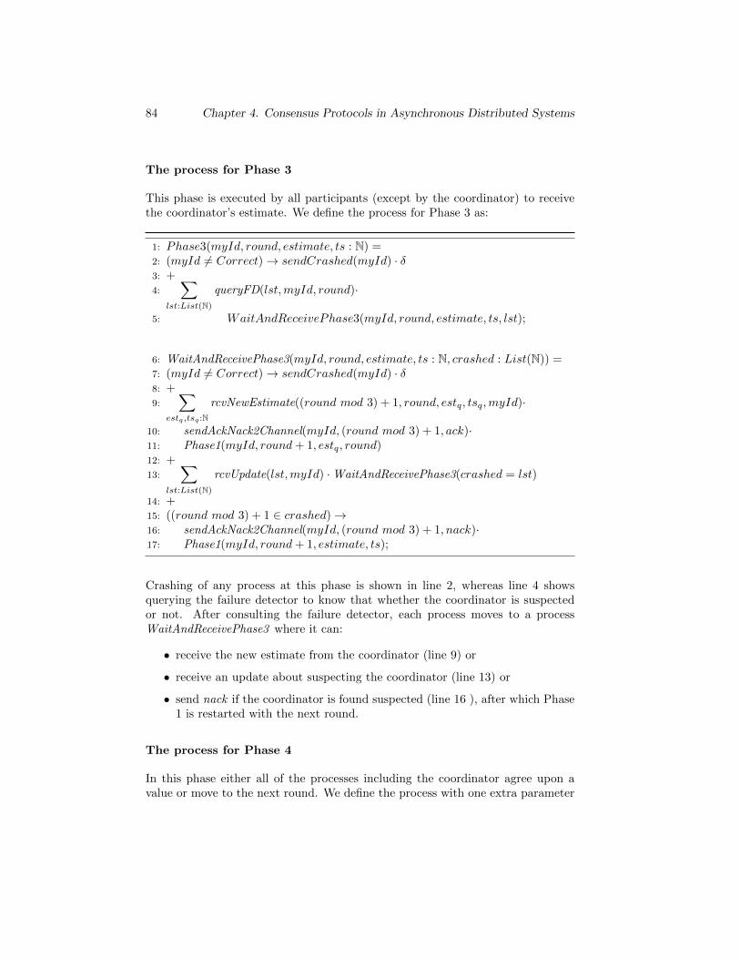
84 Chapter 4. Consensus Protocols in Asynchronous Distributed Systems
The process for Phase 3
This phase is executed by all participants (except by the coordinator) to receivethe coordinator’s estimate. We define the process for Phase 3 as:
1: Phase3(myId, round, estimate, ts : N) =2: (myId 6= Correct)→ sendCrashed(myId) · δ3: +4:
∑lst:List(N)
queryFD(lst,myId, round)·
5: WaitAndReceivePhase3(myId, round, estimate, ts, lst);
6: WaitAndReceivePhase3(myId, round, estimate, ts : N, crashed : List(N)) =7: (myId 6= Correct)→ sendCrashed(myId) · δ8: +9:
∑estq,tsq :N
rcvNewEstimate((round mod 3) + 1, round, estq, tsq,myId)·
10: sendAckNack2Channel(myId, (round mod 3) + 1, ack)·11: Phase1(myId, round+ 1, estq, round)12: +13:
∑lst:List(N)
rcvUpdate(lst,myId) ·WaitAndReceivePhase3(crashed = lst)
14: +15: ((round mod 3) + 1 ∈ crashed)→16: sendAckNack2Channel(myId, (round mod 3) + 1, nack)·17: Phase1(myId, round+ 1, estimate, ts);
Crashing of any process at this phase is shown in line 2, whereas line 4 showsquerying the failure detector to know that whether the coordinator is suspectedor not. After consulting the failure detector, each process moves to a processWaitAndReceivePhase3 where it can:
• receive the new estimate from the coordinator (line 9) or
• receive an update about suspecting the coordinator (line 13) or
• send nack if the coordinator is found suspected (line 16 ), after which Phase1 is restarted with the next round.
The process for Phase 4
In this phase either all of the processes including the coordinator agree upon avalue or move to the next round. We define the process with one extra parameter
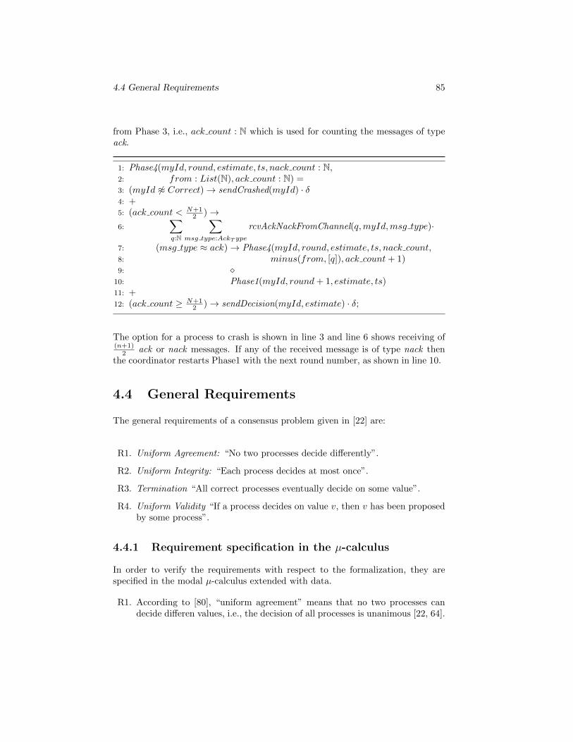
4.4 General Requirements 85
from Phase 3, i.e., ack count : N which is used for counting the messages of typeack.
1: Phase4(myId, round, estimate, ts, nack count : N,2: from : List(N), ack count : N) =3: (myId 6≈ Correct)→ sendCrashed(myId) · δ4: +5: (ack count < N+1
2 )→6:
∑q:N
∑msg type:AckT ype
rcvAckNackFromChannel(q,myId,msg type)·
7: (msg type ≈ ack)→ Phase4(myId, round, estimate, ts, nack count,8: minus(from, [q]), ack count+ 1)9: �
10: Phase1(myId, round+ 1, estimate, ts)11: +12: (ack count ≥ N+1
2 )→ sendDecision(myId, estimate) · δ;
The option for a process to crash is shown in line 3 and line 6 shows receiving of(n+1)
2 ack or nack messages. If any of the received message is of type nack thenthe coordinator restarts Phase1 with the next round number, as shown in line 10.
4.4 General Requirements
The general requirements of a consensus problem given in [22] are:
R1. Uniform Agreement: “No two processes decide differently”.
R2. Uniform Integrity: “Each process decides at most once”.
R3. Termination “All correct processes eventually decide on some value”.
R4. Uniform Validity “If a process decides on value v, then v has been proposedby some process”.
4.4.1 Requirement specification in the µ-calculus
In order to verify the requirements with respect to the formalization, they arespecified in the modal µ-calculus extended with data.
R1. According to [80], “uniform agreement” means that no two processes candecide differen values, i.e., the decision of all processes is unanimous [22, 64].
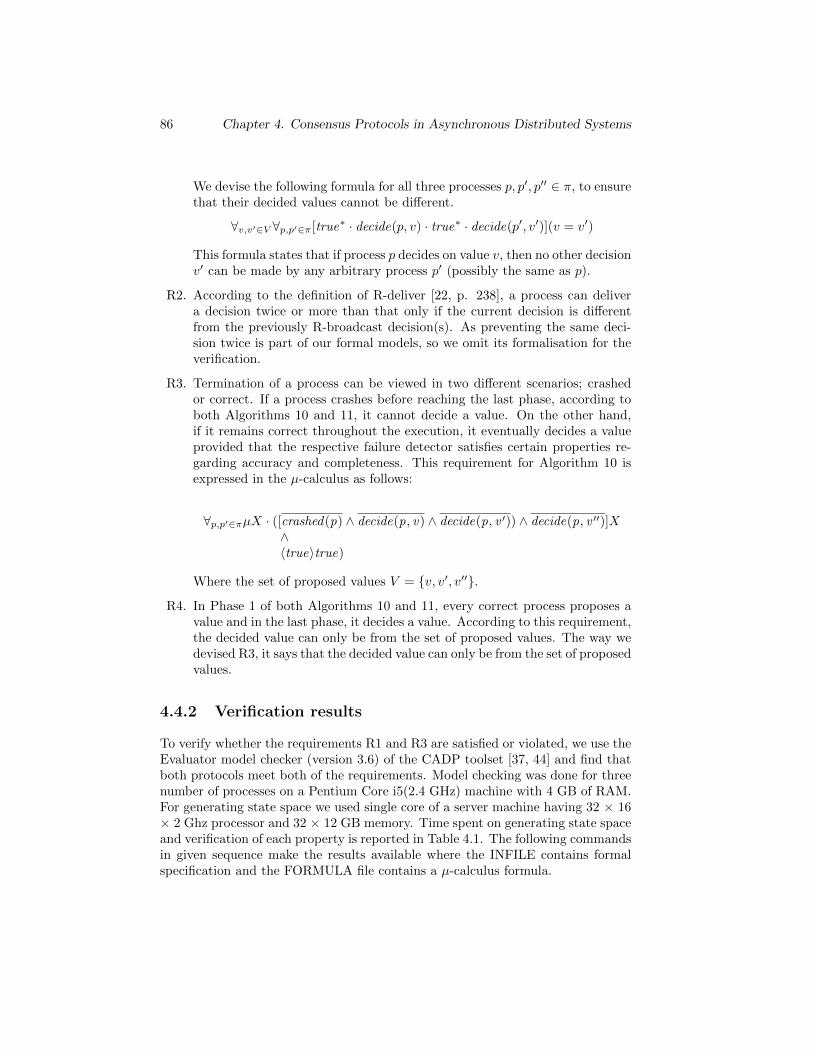
86 Chapter 4. Consensus Protocols in Asynchronous Distributed Systems
We devise the following formula for all three processes p, p′, p′′ ∈ π, to ensurethat their decided values cannot be different.
∀v,v′∈V ∀p,p′∈π[true∗ · decide(p, v) · true∗ · decide(p′, v′)](v = v′)
This formula states that if process p decides on value v, then no other decisionv′ can be made by any arbitrary process p′ (possibly the same as p).
R2. According to the definition of R-deliver [22, p. 238], a process can delivera decision twice or more than that only if the current decision is differentfrom the previously R-broadcast decision(s). As preventing the same deci-sion twice is part of our formal models, so we omit its formalisation for theverification.
R3. Termination of a process can be viewed in two different scenarios; crashedor correct. If a process crashes before reaching the last phase, according toboth Algorithms 10 and 11, it cannot decide a value. On the other hand,if it remains correct throughout the execution, it eventually decides a valueprovided that the respective failure detector satisfies certain properties re-garding accuracy and completeness. This requirement for Algorithm 10 isexpressed in the µ-calculus as follows:
∀p,p′∈πµX · ([crashed(p) ∧ decide(p, v) ∧ decide(p, v ′)) ∧ decide(p, v ′′)]X∧〈true〉true)
Where the set of proposed values V = {v, v′, v′′}.R4. In Phase 1 of both Algorithms 10 and 11, every correct process proposes a
value and in the last phase, it decides a value. According to this requirement,the decided value can only be from the set of proposed values. The way wedevised R3, it says that the decided value can only be from the set of proposedvalues.
4.4.2 Verification results
To verify whether the requirements R1 and R3 are satisfied or violated, we use theEvaluator model checker (version 3.6) of the CADP toolset [37, 44] and find thatboth protocols meet both of the requirements. Model checking was done for threenumber of processes on a Pentium Core i5(2.4 GHz) machine with 4 GB of RAM.For generating state space we used single core of a server machine having 32 × 16× 2 Ghz processor and 32 × 12 GB memory. Time spent on generating state spaceand verification of each property is reported in Table 4.1. The following commandsin given sequence make the results available where the INFILE contains formalspecification and the FORMULA file contains a µ-calculus formula.
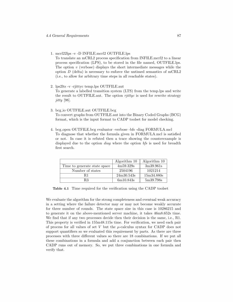
4.4 General Requirements 87
1. mcrl22lps -v -D INFILE.mcrl2 OUTFILE.lpsTo translate an mCRL2 process specification from INFILE.mcrl2 to a linearprocess specification (LPS), to be stored in the file named, OUTFILE.lps.The option v (verbose) displays the short intermediate messages while theoption D (delta) is necessary to enforce the untimed semantics of mCRL2(i.e., to allow for arbitrary time steps in all reachable states).
2. lps2lts -v -rjittyc temp.lps OUTFILE.autTo generate a labelled transition system (LTS) from the temp.lps and writethe result to OUTFILE.aut. The option rjittyc is used for rewrite strategyjitty [98].
3. bcg io OUTFILE.aut OUTFILE.bcgTo convert graphs from OUTFILE.aut into the Binary Coded Graphs (BCG)format, which is the input format to CADP toolset for model checking.
4. bcg open OUTFILE.bcg evaluator -verbose -bfs -diag FORMULA.mclTo diagnose that whether the formula given in FORMULA.mcl is satisfiedor not. In case it is refuted then a trace showing the counterexample isdisplayed due to the option diag where the option bfs is used for breadthfirst search.
Algorithm 10 Algorithm 10Time to generate state space 4m59.329s 3m39.961s
Number of states 2504196 1021214R1 24m30.543s 15m34.880sR3 6m10.843s 5m39.798s
Table 4.1 Time required for the verification using the CADP toolset
We evaluate the algorithm for the strong completeness and eventual weak accuracyin a setting where the failure detector may or may not become weakly accuratefor three number of rounds. The state space size in this case is 10286215 andto generate it on the above-mentioned server machine, it takes 46m8.652s time.We find that if any two processes decide then their decision is the same, i.e., R1.This property is verified in 155m48.115s time. For verification, we need each pairof process for all values of set V but the µ-calculus syntax for CADP does notsupport quantifiers so we evaluated this requirement by parts. As there are threeprocesses with three different values so there are 18 combinations. If we put allthese combinations in a formula and add a conjunction between each pair thenCADP runs out of memory. So, we put three combinations in one formula andverify that.
88 Chapter 4. Consensus Protocols in Asynchronous Distributed Systems
4.5 Conclusions
In fault-tolerant distributed systems, the consensus problem plays a fundamentalrole [80]. In the consensus problem, every process proposes a value and if it remainsnon-crashed during execution then it eventually decides a value with the propertythat the decision is irrevocable and unanimous [64]. Consensus cannot be solvedin asynchronous distributed systems with crash failures [40]. Hence to implementconsensus, participating processes rely on a notion of the failure detector. Afailure detector is called perfect, if it never suspects a correct process but eventuallysuspects every crashed process. In asynchronous systems, it is impossible to devisea perfect failure detector because it cannot differentiate between a crashed failureand a slow process. In [22], unreliable failure detectors are introduced to solve theconsensus problem in an asynchronous system with crash failures provided thatthey satisfy the properties of completeness and accuracy.
In this chapter, we formalized two distributed algorithms for the consensus prob-lem with their requirements. Our verification shows that all of the requirementsare satisfied by both algorithms. We presented our approach for specification ofthe protocols in the mCRL2 syntax and the requirements in the modal µ-calculus.We devised a common failure detector that satisfies weak accuracy and strongcompleteness. We model-checked the behaviour of the protocols with three par-ticipating processes.
Chapter 5
Reconstruction andVerification of GroupMembership Protocols
Reconstruction and Verification of Group Membership Protocols. In: Proceedings of the10th International Workshop on Automated Verification of Critical Systems (AVOCS’10)
90 Chapter 5. Group Membership Protocols
5.1 Introduction
Group membership protocols [28] form an important foundation for distributedsystems, allowing the different nodes in such a system to maintain a consistentview on which nodes are currently active. Naturally, a group membership protocolmust be able to deal with nodes deliberately entering and leaving the currentconfiguration set. However, it is also important for a group membership protocolto be fault-tolerant; due to faulty behaviour of nodes or of the network, nodesmight also be considered inactive.
Pioneering algorithms among group membership protocols are the ones presentedby Amir et al. in [3]; these were the first group membership protocols with supportfor partitioning [28]. Our initial intention was to formally specify and verify the al-gorithms presented in [3]. However, we soon found numerous ambiguities making astraightforward formal specification of these algorithms virtually impossible. Sinceour attempts to communicate with the authors of [3] were not successful, we wereforced to reconstruct these algorithms by systematically enumerating, trying andverifying different possible interpretation of these algorithms. Hence, in this chap-ter, we present two group membership algorithms inspired by [3], formally specifythem in the process algebra mCRL2 [49] and prove them correct with respect tothe requirements formalized in terms of monitor processes. In our presentation, weshow how we have come up with them and why some other (seemingly simpler andmore faithful) interpretations of the algorithms in [3] violate the basic propertiesrequired for a group membership algorithm.
The algorithms presented in [3] are part of a larger distributed system frameworkcalled Transis [5]. They essentially rely on Transis in that they use some servicesprovided by Transis and also augment its functionality by providing facilities forgroup membership. Hence, in our formalization, we not only build a formal modelof these algorithms, but also develop a formal layer of abstraction presenting thebehaviour of Transis. An extended version of this chapter is presented in [12].
Structure of the chapter. The rest of this chapter is organised as follows.In Section 5.2 the architecture of the distributed system and protocols studiedin this chapter is presented. In Section 2.2 an overview of the process algebramCRL2 used for our formalization is given. An informal description of Transisand an excerpt of its formal specification is provided in Section 5.3. Section 5.4is dedicated to the membership algorithms and their formalisation. In Section 5.5the requirements on the algorithms are defined, formalised, and verified on theformal models. A brief overview of the related work is given in Section 5.6. Thechapter is concluded in Section 5.7.
5.2 Architecture of the Distributed System 91
5.2 Architecture of the Distributed System
In short, the goal of the membership protocol is to keep a consistent view of thegroup among the member nodes by handling faults, i.e., failing nodes or commu-nication channels (to be excluded from the group’s view), and joins, nodes joiningthe network (to be added to the group’s view).
The original paper [3] specifies the membership protocol as a combination of afault-handling mechanism and a join-handling mechanism, running on top of acommunication subsystem called Transis. Both mechanisms are first explainedseparately, and then combined (only requiring modification of the join mechanism)to form the full membership protocol.
Essentially, the feature of Transis used in the specification of membership algo-rithms is a service called causal multicast. This service broadcasts messages to agroup of recipients, and guarantees that the delivery of messages at their desti-nation preserves a certain ordering, the causal order (a formal description of thisorder is given in the remainder of this chapter). Preserving this order involves adirected acyclic graph, or DAG, of which the nodes are messages and the edgesare direct causal orderings. This DAG is constructed locally at every node. Aseach node is supposed to construct the exact same graph, the local copies are oftencollectively referred to as ‘the DAG’.
The first thing we would like to establish is what status the membership protocolhas. Is it part of Transis, does it operate on top of Transis, or is it an independentlyoperating application? The following quotes from [3] seem to indicate that noneof the above are exactly true.
The membership protocol operates above the Transis communicationlayer, such that message arrival order within the protocol preservescausality. [3, p. 295]
From [4, 3, 5] we deduce that messages are inserted into the DAG by Transis onarrival. Messages are delivered to the upper level by Transis when they becomedeliverable in the DAG. The first quote above suggests that the membership pro-tocol therefore has to wait until a message becomes deliverable in the DAG. Thefollowing quote however implies that the protocol must be able to handle messagesbefore they are delivered.
When a FA message is inserted into the DAG, the faults algorithmmarks it nondeliverable. [3, p. 298]
The next quote reveals the cause of the confusion: the boundary between Transisand the membership protocol is not a strict one.
The Transis communication sub-system [...] delivers the messages to
92 Chapter 5. Group Membership Protocols
the upper level. The services use different delivery criteria on the mes-sages in the DAG. In some cases, the membership protocol interfereswith the delivery of messages, as we shall see below. [3, p. 296]
We choose to resolve the above inconsistency by ignoring the first quote, whichsuggests a strict separation between Transis and the protocols and assumes causalordering on the arrival of messages. As we will see in the rest of this document, itseems likely that the membership protocol uses Transis to keep track of the causalorder of messages, but does in fact deal with messages that arrive out of causalorder.
In order to make the formalisation of the protocol easier, we would like to de-fine an interface between Transis and the membership protocol. As mentionedbefore, the membership protocol interferes with the normal operation of Transis.In an attempt to formalise this interference, we assume existence of the followingmechanisms:
• Transis keeps a list of senders from which it will refuse to receive messages.The membership protocol may alter this list at any given time. We need thismechanism because the membership protocol needs to “instruct Transis todisallow any message from f set to enter the DAG” ([3, p. 299], fig. 3).
• Transis distinguishes between membership protocol messages and other mes-sages. Since the protocol messages arrive at the membership protocol, butuser messages don’t, this must be the case.
• The membership protocol receives the IDs of the senders of received mes-sages, so that it may recognise nodes that are not in the current configurationset. We need this to identify ‘foreign messages’ ([3, p. 306], fig. 6).
• The membership protocol receives protocol-specific messages from Transisupon reception from the channel. As discussed above, the messages must behandled on arrival, not on delivery.
• The membership protocol may assign markings to messages in the DAG. Thebehaviour of Transis is defined in terms of these markings. This marking isdone on in Figures 3, 5 and 7 on pages 299, 305 and 307 respectively.
The above mechanisms provide all the functionality that the membership protocolneeds to influence the behaviour of Transis. We have chosen these mechanismssuch that Transis’ behaviour can be defined independently of the membershipprotocol. The only exception to this rule is that Transis distinguishes membershipprotocol messages from other messages.
Figure 5.1 shows the context of the membership protocol on a single node. Themembership protocol itself only communicates with Transis, which in turn mayaccept and deliver messages from and to the user (the application layer), and which
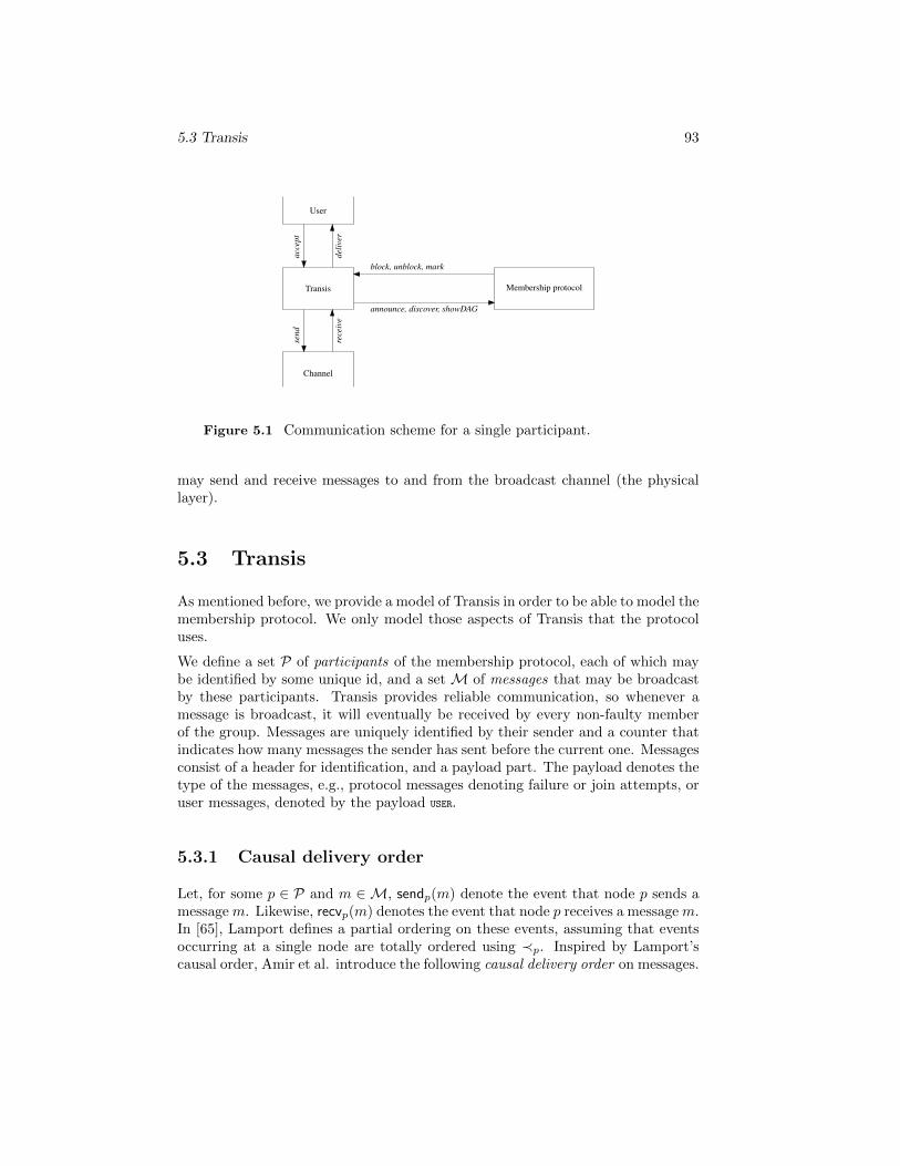
5.3 Transis 93
Transis Membership protocol
Channel
User
block, unblock, mark
announce, discover, showDAGac
cept
deliv
er
send
rece
ive
Figure 5.1 Communication scheme for a single participant.
may send and receive messages to and from the broadcast channel (the physicallayer).
5.3 Transis
As mentioned before, we provide a model of Transis in order to be able to model themembership protocol. We only model those aspects of Transis that the protocoluses.
We define a set P of participants of the membership protocol, each of which maybe identified by some unique id, and a set M of messages that may be broadcastby these participants. Transis provides reliable communication, so whenever amessage is broadcast, it will eventually be received by every non-faulty memberof the group. Messages are uniquely identified by their sender and a counter thatindicates how many messages the sender has sent before the current one. Messagesconsist of a header for identification, and a payload part. The payload denotes thetype of the messages, e.g., protocol messages denoting failure or join attempts, oruser messages, denoted by the payload USER.
5.3.1 Causal delivery order
Let, for some p ∈ P and m ∈ M, sendp(m) denote the event that node p sends amessage m. Likewise, recvp(m) denotes the event that node p receives a message m.In [65], Lamport defines a partial ordering on these events, assuming that eventsoccurring at a single node are totally ordered using ≺p. Inspired by Lamport’scausal order, Amir et al. introduce the following causal delivery order on messages.
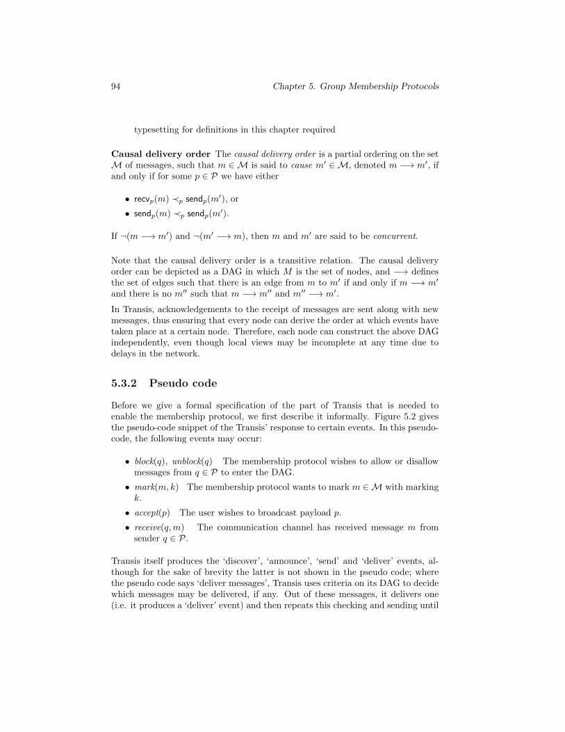
94 Chapter 5. Group Membership Protocols
typesetting for definitions in this chapter required
Causal delivery order The causal delivery order is a partial ordering on the setM of messages, such that m ∈M is said to cause m′ ∈M, denoted m −→ m′, ifand only if for some p ∈ P we have either
• recvp(m) ≺p sendp(m′), or
• sendp(m) ≺p sendp(m′).
If ¬(m −→ m′) and ¬(m′ −→ m), then m and m′ are said to be concurrent.
Note that the causal delivery order is a transitive relation. The causal deliveryorder can be depicted as a DAG in which M is the set of nodes, and −→ definesthe set of edges such that there is an edge from m to m′ if and only if m −→ m′
and there is no m′′ such that m −→ m′′ and m′′ −→ m′.
In Transis, acknowledgements to the receipt of messages are sent along with newmessages, thus ensuring that every node can derive the order at which events havetaken place at a certain node. Therefore, each node can construct the above DAGindependently, even though local views may be incomplete at any time due todelays in the network.
5.3.2 Pseudo code
Before we give a formal specification of the part of Transis that is needed toenable the membership protocol, we first describe it informally. Figure 5.2 givesthe pseudo-code snippet of the Transis’ response to certain events. In this pseudo-code, the following events may occur:
• block(q), unblock(q) The membership protocol wishes to allow or disallowmessages from q ∈ P to enter the DAG.
• mark(m, k) The membership protocol wants to mark m ∈M with markingk.
• accept(p) The user wishes to broadcast payload p.
• receive(q,m) The communication channel has received message m fromsender q ∈ P.
Transis itself produces the ‘discover’, ‘announce’, ‘send’ and ‘deliver’ events, al-though for the sake of brevity the latter is not shown in the pseudo code; wherethe pseudo code says ‘deliver messages’, Transis uses criteria on its DAG to decidewhich messages may be delivered, if any. Out of these messages, it delivers one(i.e. it produces a ‘deliver’ event) and then repeats this checking and sending until
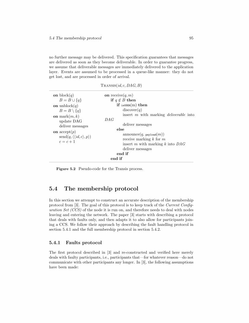
5.4 The membership protocol 95
no further message may be delivered. This specification guarantees that messagesare delivered as soon as they become deliverable. In order to guarantee progress,we assume that deliverable messages are immediately delivered to the applicationlayer. Events are assumed to be processed in a queue-like manner: they do notget lost, and are processed in order of arrival.
Transis(id, c,DAG, B)
on block(q)B = B ∪ {q}
on unblock(q)B = B \ {q}
on mark(m, k)update DAGdeliver messages
on accept(p)send(q, 〈〈id, c〉, p〉)c = c+ 1
on receive(q,m)if q /∈ B then
if isUSER(m) thendiscover(q)insert m with marking deliverable into
DAGdeliver messages
elseannounce(q, payload(m))receive marking k for minsert m with marking k into DAGdeliver messages
end ifend if
Figure 5.2 Pseudo-code for the Transis process.
5.4 The membership protocol
In this section we attempt to construct an accurate description of the membershipprotocol from [3]. The goal of this protocol is to keep track of the Current Config-uration Set (CCS) of the node it is run on, and therefore needs to deal with nodesleaving and entering the network. The paper [3] starts with describing a protocolthat deals with faults only, and then adapts it to also allow for participants join-ing a CCS. We follow their approach by describing the fault handling protocol insection 5.4.1 and the full membership protocol in section 5.4.2.
5.4.1 Faults protocol
The first protocol described in [3] and re-constructed and verified here merelydeals with faulty participants, i.e., participants that—for whatever reason—do notcommunicate with other participants any longer. In [3], the following assumptionshave been made:
96 Chapter 5. Group Membership Protocols
• Messages are not delayed indefinitely.
• Communication breaks can be detected.
• Initially, all participants in CCS know the contents of CCS .
We note that the CCS may differ per node, as the network may be partitioned.
Pseudo-code
The idea behind the faults protocol is quite simple. Once a communication breakwith another participant is detected, this information is shared with the otherparticipants by means of an FA (fault) message. Each node q has its own set Fof participants that it thinks have failed, and a list LastF that contains, for eachparticipant q′, the set of participants that q knows are in the set F of q′. When allparticipants have the same F set, then this will eventually cause LastF to containonly sets equal to F , and participants can then locally conclude that consensus isreached.
Figure 5.3 The faults protocol description.
The original pseudo-code for the faults protocol is shown in Figure 5.3 and consistsof four if -statements. However, the semantics of those four if -statements seems to
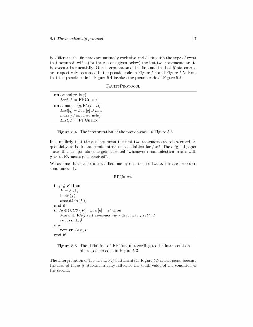
5.4 The membership protocol 97
be different; the first two are mutually exclusive and distinguish the type of eventthat occurred, while (for the reasons given below) the last two statements are tobe executed sequentially. Our interpretation of the first and the last if -statementsare respectively presented in the pseudo-code in Figure 5.4 and Figure 5.5. Notethat the pseudo-code in Figure 5.4 invokes the pseudo-code of Figure 5.5.
FaultsProtocol
on commbreak(q)Last , F = FPCheck
on announce(q,FA(f set))Last [q] = Last [q] ∪ f setmark(id,undeliverable)Last , F = FPCheck
Figure 5.4 The interpretation of the pseudo-code in Figure 5.3.
It is unlikely that the authors mean the first two statements to be executed se-quentially, as both statements introduce a definition for f set. The original paperstates that the pseudo-code gets executed “whenever communication breaks withq or an FA message is received”.
We assume that events are handled one by one, i.e., no two events are processedsimultaneously.
FPCheck
if f 6⊆ F thenF = F ∪ fblock(f)accept(FA(F ))
end ifif ∀q ∈ (CCS \ F ) : Last [q] = F then
Mark all FA(f set) messages slow that have f set ⊆ Freturn ⊥, ∅
elsereturn Last , F
end if
Figure 5.5 The definition of FPCheck according to the interpretationof the pseudo-code in Figure 5.3
The interpretation of the last two if -statements in Figure 5.5 makes sense becausethe first of these if statements may influence the truth value of the condition ofthe second.
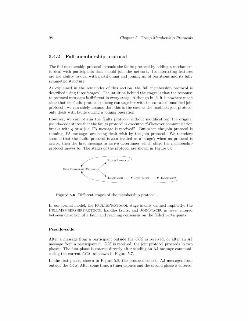
98 Chapter 5. Group Membership Protocols
5.4.2 Full membership protocol
The full membership protocol extends the faults protocol by adding a mechanismto deal with participants that should join the network. Its interesting featuresare the ability to deal with partitioning and joining up of partitions and its fullysymmetric structure.
As explained in the remainder of this section, the full membership protocol isdescribed using three ‘stages’. The intuition behind the stages is that the responseto protocol messages is different in every stage. Although in [3] it is nowhere madeclear that the faults protocol is being run together with the so-called ‘modified joinprotocol’, we can safely assume that this is the case as the modified join protocolonly deals with faults during a joining operation.
However, we cannot run the faults protocol without modification: the originalpseudo-code states that the faults protocol is executed “Whenever communicationbreaks with q or a [sic] FA message is received”. But when the join protocol isrunning, FA messages are being dealt with by the join protocol. We thereforeassume that the faults protocol is also treated as a ‘stage’; when no protocol isactive, then the first message to arrive determines which stage the membershipprotocol moves to. The stages of the protocol are shown in Figure 5.6.
FullMembershipProtocol
FaultsProtocol
JoinStage0 JoinStage1 JoinStage2
Figure 5.6 Different stages of the membership protocol.
In our formal model, the FaultsProtocol stage is only defined implicitly; theFullMembershipProtocol handles faults, and JoinStage0 is never enteredbetween detection of a fault and reaching consensus on the failed participants.
Pseudo-code
After a message from a participant outside the CCS is received, or after an AJmessage from a participant in CCS is received, the join protocol proceeds in twophases. The first phase is entered directly after sending an AJ message communi-cating the current CCS , as shown in Figure 5.7.
In the first phase, shown in Figure 5.8, the protocol collects AJ messages fromoutside the CCS . After some time, a timer expires and the second phase is entered.
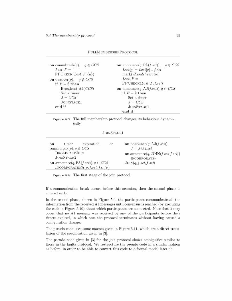
5.4 The membership protocol 99
FullMembershipProtocol
on commbreak(q), q ∈ CCSLast , F =FPCheck(Last , F, {q})
on discover(q), q /∈ CCSif F = ∅ then
Broadcast AJ(CCS)Set a timerJ = CCSJoinStage1
end if
on announce(q,FA(f set)), q ∈ CCSLast [q] = Last [q] ∪ f setmark(id,undeliverable)Last , F =FPCheck(Last , F, f set)
on announce(q,AJ(j set)), q ∈ CCSif F = ∅ then
Set a timerJ = CCSJoinStage1
end if
Figure 5.7 The full membership protocol changes its behaviour dynami-cally.
JoinStage1
on timer expiration orcommbreak(q), q ∈ CCS
BroadcastJoinJoinStage2
on announce(q,FA(f set)), q ∈ CCSIncorporateFA(q, f set, fJ , fF )
on announce(q,AJ(j set))J = J ∪ j set
on announce(q, JOIN(j set, f set))Incorporate-
Join(q, j set, f set)
Figure 5.8 The first stage of the join protocol.
If a communication break occurs before this occasion, then the second phase isentered early.
In the second phase, shown in Figure 5.9, the participants communicate all theinformation from the received AJ messages until consensus is reached (by executingthe code in Figure 5.10) about which participants are connected. Note that it mayoccur that no AJ message was received by any of the participants before theirtimers expired, in which case the protocol terminates without having caused aconfiguration change.
The pseudo code uses some macros given in Figure 5.11, which are a direct trans-lation of the specification given in [3].
The pseudo code given in [3] for the join protocol shows ambiguities similar tothose in the faults protocol. We restructure the pseudo code in a similar fashionas before, in order to be able to convert this code to a formal model later on.
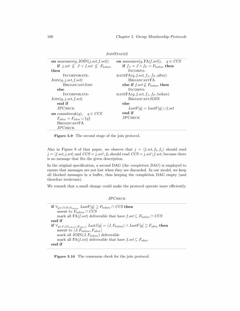
100 Chapter 5. Group Membership Protocols
JoinStage2
on announce(q, JOIN(j set, f set))if j set 6⊆ J ∨ f set 6⊆ Fbefore
thenIncorporate-
Join(q, j set, f set)BroadcastJoin
elseIncorporate-
Join(q, j set, f set)end ifJPCheck
on commbreak(q), q ∈ CCSFafter = Fafter ∪ {q}BroadcastFAJPCheck
on announce(q,FA(f set)), q ∈ CCSif fJ = J ∧ fF = Fbefore then
Incorpo-rateFA(q, f set, fJ , fF , after)
BroadcastFAelse if f set 6⊆ Fbefore then
Incorpo-rateFA(q, f set, fJ , fF ,before)
BroadcastJOINelse
LastF [q] = LastF [q] ∪ f setend ifJPCheck
Figure 5.9 The second stage of the join protocol.
Also in Figure 8 of that paper, we observe that j = 〈f set, fb, fa〉 should readj = 〈f set, j set〉 and CCS = j set\fb should read CCS = j set\ f set, because thereis no message that fits the given description.
In the original specification, a second DAG (the completion DAG) is employed toensure that messages are not lost when they are discarded. In our model, we keepall blocked messages in a buffer, thus keeping the completion DAG empty (andtherefore irrelevant).
We remark that a small change could make the protocol operate more efficiently.
JPCheck
if ∀q∈CCS\FbeforeLastF [q] ⊇ Fbefore ∩ CCS then
assent to Fbefore ∩ CCSmark all FA(f set) deliverable that have f set ⊆ Fbefore ∩ CCS
end ifif ∀q∈J\(Fbefore∪Fafter) LastJ [q] = 〈J, Fbefore〉 ∧ LastF [q] ⊇ Fafter then
assent to 〈J, Fbefore, Fafter〉mark all JOIN(J, Fbefore) deliverablemark all FA(f set) deliverable that have f set ⊆ Fafter
end if
Figure 5.10 The consensus check for the join protocol.
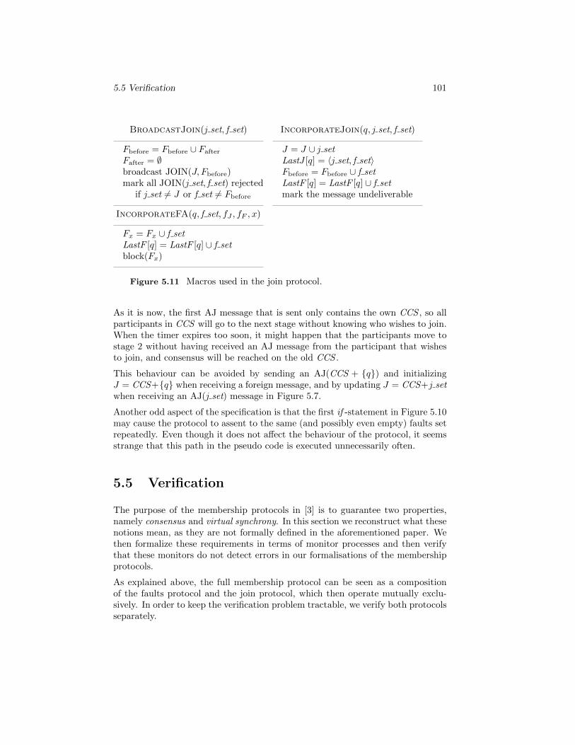
5.5 Verification 101
BroadcastJoin(j set, f set)
Fbefore = Fbefore ∪ Fafter
Fafter = ∅broadcast JOIN(J, Fbefore)mark all JOIN(j set, f set) rejected
if j set 6= J or f set 6= Fbefore
IncorporateFA(q, f set, fJ , fF , x)
Fx = Fx ∪ f setLastF [q] = LastF [q] ∪ f setblock(Fx)
IncorporateJoin(q, j set, f set)
J = J ∪ j setLastJ [q] = 〈j set, f set〉Fbefore = Fbefore ∪ f setLastF [q] = LastF [q] ∪ f setmark the message undeliverable
Figure 5.11 Macros used in the join protocol.
As it is now, the first AJ message that is sent only contains the own CCS , so allparticipants in CCS will go to the next stage without knowing who wishes to join.When the timer expires too soon, it might happen that the participants move tostage 2 without having received an AJ message from the participant that wishesto join, and consensus will be reached on the old CCS .
This behaviour can be avoided by sending an AJ(CCS + {q}) and initializingJ = CCS+{q} when receiving a foreign message, and by updating J = CCS+j setwhen receiving an AJ(j set) message in Figure 5.7.
Another odd aspect of the specification is that the first if -statement in Figure 5.10may cause the protocol to assent to the same (and possibly even empty) faults setrepeatedly. Even though it does not affect the behaviour of the protocol, it seemsstrange that this path in the pseudo code is executed unnecessarily often.
5.5 Verification
The purpose of the membership protocols in [3] is to guarantee two properties,namely consensus and virtual synchrony. In this section we reconstruct what thesenotions mean, as they are not formally defined in the aforementioned paper. Wethen formalize these requirements in terms of monitor processes and then verifythat these monitors do not detect errors in our formalisations of the membershipprotocols.
As explained above, the full membership protocol can be seen as a compositionof the faults protocol and the join protocol, which then operate mutually exclu-sively. In order to keep the verification problem tractable, we verify both protocolsseparately.
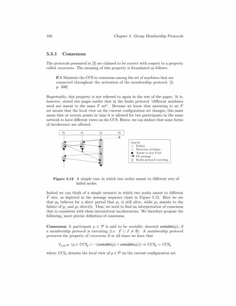
102 Chapter 5. Group Membership Protocols
5.5.1 Consensus
The protocols presented in [3] are claimed to be correct with respect to a propertycalled consensus. The meaning of this property is formulated as follows:
P.1 Maintain the CCS in consensus among the set of machines that areconnected throughout the activation of the membership protocol. [3,p. 300]
Regrettably, this property is not referred to again in the rest of the paper. It is,however, stated two pages earlier that in the faults protocol “different machinesneed not assent to the same F set”. Because we know that assenting to an Fset means that the local view on the current configuration set changes, this mustmean that at certain points in time it is allowed for two participants in the samenetwork to have different views on the CCS. Hence, we can deduce that some formsof incoherence are allowed.
p0 p1 p2 p3
Legend× Failure# Detection of failure Assent to new F-set
FA messageFaults protocol executing
Figure 5.12 A simple case in which two nodes assent to different sets offailed nodes.
Indeed we can think of a simple scenario in which two nodes assent to differentF sets, as depicted in the message sequence chart in Figure 5.12. Here we seethat p0 believes for a short period that p1 is still alive, while p2 assents to thefailure of p1 and p3 directly. Thus, we need to find an interpretation of consensusthat is consistent with these intermittent incoherencies. We therefore propose thefollowing, more precise definition of consensus.
Consensus A participant p ∈ P is said to be unstable, denoted unstable(p), ifa membership protocol is executing (i.e. F ∪ J 6= ∅). A membership protocolpreserves the property of consensus if at all times we have that
∀p,q∈P (q ∈ CCSp ∧ ¬ (unstable(p) ∨ unstable(q)))⇒ CCSp = CCSq
where CCSp denotes the local view of p ∈ P on the current configuration set.
5.5 Verification 103
Note that this definition allows for the existence of cliques (due to partitioning)and for nodes not assenting to the same fault or join sets. In particular, thesituation in Figure 5.12 is allowed.
5.5.2 Virtual synchrony
Another aspect informally described in [3] is the notion of virtual synchrony. Inthe introduction, the following descriptions can be found.
Virtual-synchrony. It guarantees that members of the same configura-tion receive the same set of messages between every pair of configura-tion changes. [3, p. 293]
The technical report [4] describing the membership protocols refers to [92] as thesource of their notion of virtual synchrony. However, the latter paper only definesvirtual synchrony in terms of processes ‘observing consistent delivery orders’, andnot in terms of delivering messages in between configuration changes, like in thesecond quote above. This seems to indicate that all messages should be sent inTransis’ causal multicast mode, but that conflicts with the following quote.
The Basic service of Transis overcomes arbitrary communication de-lays and message losses and guarantees fast delivery of messages atall of the currently connected destinations. The membership protocolautomatically maintains the set of currently connected machines insidethe broadcast domain. [3, p. 293]
The description of causal multicast from the next quote suggests that in basicmulticast mode, delivery order does not preserve causality:
1. Basic multicast: guarantees delivery of the message at all theconnected sites. This service delivers the message immediatelyfrom the DAG to the upper level.
2. Causal multicast: guarantees that delivery order preserves causal-ity. [3, p. 296]
Assuming that messages are delivered as soon as they have been inserted into theDAG however immediately leads to problems: if a configuration change happenssimultaneously at all nodes, but one of the nodes receives a regular message beforethat change while another receives that same message only later, then virtualsynchrony (as described in the second quote) is violated.
In the proof of the faults protocol, we find the following:
104 Chapter 5. Group Membership Protocols
If a message follows any of the messages in Electorsp(f), it is deliveredonly after the configuration change of f . [3, p. 300]
Then p and q deliver the same set of causal messages [...] [3, p. 300]
These quotes seem to indicate that we are dealing with causal delivery order.
The above quote speaks of “causal messages”, which seems to indicate that thereare other types of messages being delivered too. We therefore assume that thebasic multicast and causal multicast services can be used independently.
Remember that the faults and join protocol change the CCS on delivery of FAand JOIN messages. Call these messages configuration changing messages. Tryingto formulate a property in the spirit of [92] that matches [3], we define virtualsynchrony as follows:
Virtual synchrony The network is virtually synchronous if and only if
• configuration changing messages are delivered in the same order at everynode, and between every two delivered, and
• if m1 and m2 are configuration changing messages, and a node delivers amessage m that was sent using the causal multicast service after m1 butbefore m2, then all other nodes in the current CCS deliver m after m1 andbefore m2.
5.5.3 Requirements monitoring
In order to verify that the faults and join protocols have the desired properties,we construct monitor processes that produce an error action upon violation ofthe requirement they encode. We check reachability of this action on the systemcomposed in parallel with the monitor processes.
The consensus monitor synchronises with the system whenever a process crashesand whenever a process starts or stops executing the faults (resp. join) protocol(i.e. whenever a process assents to a configuration change). When no processes areexecuting the faults (join) protocol, we require that the processes have assentedto the same changes. If not, then an error action is possible.
The virtual synchrony monitor synchronises with the system whenever a processdelivers a message. For every process, the monitor process keeps a list of deliveredmessages. Whenever these lists violate the definition of Virtual Synchrony inSection 5.5.2, an error action is possible.
To check the faults protocol, we model a network consisting of three nodes, of whichone can crash. For the join protocol, we start with a network that is partitionedinto a clique of two nodes, of which one may crash at any given time, and a cliqueconsisting of a single node. Every node is allowed to send a user message (i.e. a
5.6 Related Work 105
message that has no meaning for the protocol, but that is sent using the causalmulticast service) once.
Results
The specification of the protocols in mCRL2 are transformed to linear processspecification format [49] using the mcrl22lps tool. We then check reachability ofthe error action with the lps2lts tool. If an error action is reachable, then thistool will produce a trace that leads to this action.
Verification was done using a Q9400 Intel R© CoreTM 2 Quad CPU (of which onecore is used) and 3GB of memory using the mCRL2 toolset development version(revision 7884).
For the faults protocol, it took 28 minutes and 55 seconds to exhaust the statespace comprising about 1.2 million states (this state space is the result of thecomposition of the monitor process and the protocol specification). We couldsuccessfully verify both consensus and virtual synchrony for our formal model ofthe faults protocol.
For the join protocol, the state-space proved to be too large to be verified in afew days. Hence, we resorted to bounded model-checking by limiting the depth orthe breadth of the search algorithm. Using the limit on the depth, we successfullyverified over 4 million system states (22 levels, i.e. 22 ‘steps’ in the protocol),and over 113 million for the consensus property alone. Using the highway search(breadth-constrained) algorithm [36], we could verify 1000 randomly chosen stateson every level of the state space.
For the complete models of the protocols and the monitors see Appendices C.1and C.2.
5.6 Related Work
An overview of different group membership protocols can be found in [28], where[3] is cited as the first group membership protocol dealing partitioning. We havegathered and used scattered information about the algorithms of [3] and its un-derlying Transis system from [3, 4, 5].
In the literature several attempts have been made to formalise and verify groupmembership protocols. The first one, that we are aware of is [86], where a groupmembership algorithm has been formalised and verified. Later in [7], a number offlaws were identified in the formalisation of [86] and a new formal verification ofthe corrected version has been presented. Along the same lines, in [16] a formalspecification of a group membership protocol is presented.
106 Chapter 5. Group Membership Protocols
5.7 Conclusions
We provided a formal specification of the group membership protocols presentedin [3] and their correctness properties and model-checked the properties on the for-mal specifications. For the formalisation, we had to disambiguate the descriptionprovided in the original paper and in order to realise the properties, we had totry different interpretations of the informal text. The process of disambiguationhas been laborious and rather difficult; it often appeared from the formal analysisthat the most natural interpretation of the text led to inconsistencies or incorrectbehaviour and thus, less faithful interpretations of the text had to be used in orderto reconstruct correct group membership protocols. We could successfully model-check our final specification of the faults protocol. For the join protocol, we hadto resort to bounded model-checking, which did not indicate any counterexampleafter both a highway search (breadth-constrained) as well as depth-constrainedsearch.
We have verified these protocols for a fixed number of participants; extending theresults to an arbitrary number of participants means of parametric verificationtechniques remains as an avenue for future work.
Chapter 6
Formal Verification ofEfficient Algorithms toImplement UnreliableFailure Detectors inPartially SynchronousSystems
Formal Verification of Unreliable Failure Detectors in Partially Synchronous Systems. CS-Report 11-12, Eindhoven University of Technology, 2011.
108 Chapter 6. Unreliable Failure Detectors in Partially Synchronous Systems
6.1 Introduction
Distributed systems are vulnerable to faults such as the crash of the participatingprocesses or the communication media among them. A key challenge is to designdistributed failure detectors that allow processes to distinguish slow processes fromthose which have crashed. It is important that these detectors are accurate, i.e.,do not suspect correct processes, and complete, i.e., do suspect crashed ones.Given their non-trivial design, it is highly desirable to validate that these protocolssatisfy their required or claimed properties. M. Larrea et al. introduce “efficientalgorithms to implement failure detectors in partially synchronous systems” in [70],whose formal verification forms the subject matter of this chapter. An extendedversion of this chapter is presented in [14].
In this chapter, we formally verify the four algorithms proposed in [70]. Each algo-rithm is specified formally as a network of timed automata [2] and is verified withrespect to completeness and accuracy properties which are already introduced inChapter 4. In this Chapter, we discuss two more classes of properties for thesealgorithms. Using the model-checking tool UPPAAL, we detect and report occur-rences of deadlock (for all algorithms) between each pair of communicating andnon-faulty nodes due to buffer overflow in the communication channels with arbi-trarily large buffers. We propose one solution for deadlock avoidance. Moreover,we use one of the algorithms studied in this chapter as a measure to comparethe effectiveness of three model-checking tools, namely, UPPAAL, mCRL2 andFDR2. We also show that the deadlock-free version of all algorithms satisfy theircompleteness and accuracy properties if the required number of processes remainoperational.
6.1.1 Types of unreliable failure detectors
A failure detector is called unreliable, if it can mistakenly report a correct process(a process that remains operational during the protocol) as faulty (also known assuspected or crashed; suspected refers to the belief of the detector and crashedrefers to the type of purported failure). Chandra and Toueg proposed differentclasses of unreliable failure detectors in [22] (see also Chapter 4) to guaranteetwo essential properties, namely, completeness and accuracy. Completeness isabout suspecting each faulty process and accuracy concerns not suspecting anycorrect process. These properties are further classified into weak and strong as:strong completeness, weak completeness, eventual strong accuracy and eventualweak accuracy. We have already discussed two of these properties in Chapter 4;the remaining two are defined below:
1. Weak completeness: Eventually every faulty process is permanently sus-pected by some non-faulty process.
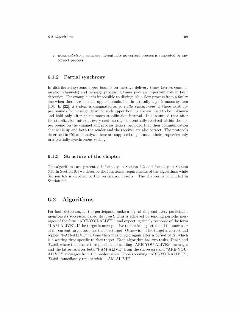
6.2 Algorithms 109
2. Eventual strong accuracy : Eventually no correct process is suspected by anycorrect process.
6.1.2 Partial synchrony
In distributed systems upper bounds on message delivery times (across commu-nication channels) and message processing times play an important role in faultdetection. For example, it is impossible to distinguish a slow process from a faultyone when there are no such upper bounds, i.e., in a totally asynchronous system[40]. In [22], a system is designated as partially synchronous, if there exist up-per bounds for message delivery; such upper bounds are assumed to be unknownand hold only after an unknown stabilization interval. It is assumed that afterthe stabilization interval, every sent message is eventually received within the up-per bound on the channel and process delays, provided that their communicationchannel is up and both the sender and the receiver are also correct. The protocolsdescribed in [70] and analyzed here are supposed to guarantee their properties onlyin a partially synchronous setting.
6.1.3 Structure of the chapter
The algorithms are presented informally in Section 6.2 and formally in Section6.3. In Section 6.4 we describe the functional requirements of the algorithms whileSection 6.5 is devoted to the verification results. The chapter is concluded inSection 6.6.
6.2 Algorithms
For fault detection, all the participants make a logical ring and every participantmonitors its successor, called its target. This is achieved by sending periodic mes-sages of the form “ARE-YOU-ALIVE?” and expecting timely response of the form“I-AM-ALIVE”. If the target is unresponsive then it is suspected and the successorof the current target becomes the new target. Otherwise, if the target is correct andreplies “I-AM-ALIVE” in time then it is pinged again after a period of ∆, whichis a waiting time specific to that target. Each algorithm has two tasks, Task1 andTask2, where the former is responsible for sending “ARE-YOU-ALIVE?” messagesand the latter receives both “I-AM-ALIVE” from the successors and “ARE-YOU-ALIVE?” messages from the predecessors. Upon receiving “ARE-YOU-ALIVE?”,Task2 immediately replies with “I-AM-ALIVE”.
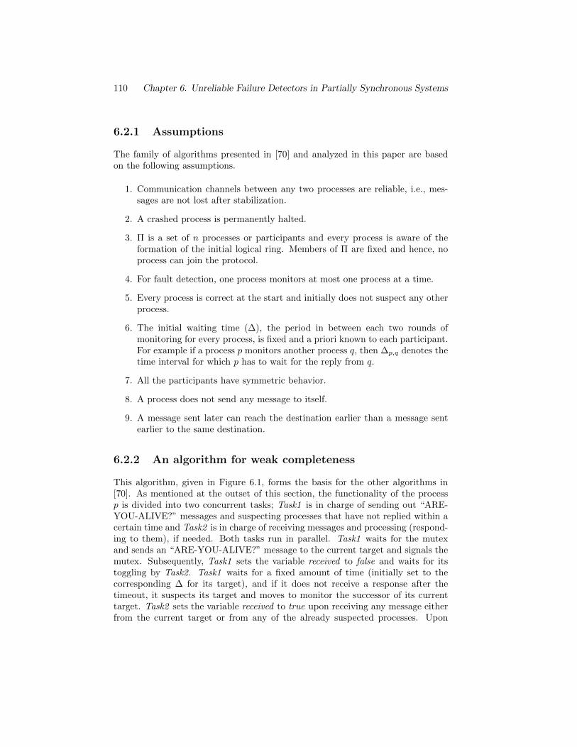
110 Chapter 6. Unreliable Failure Detectors in Partially Synchronous Systems
6.2.1 Assumptions
The family of algorithms presented in [70] and analyzed in this paper are basedon the following assumptions.
1. Communication channels between any two processes are reliable, i.e., mes-sages are not lost after stabilization.
2. A crashed process is permanently halted.
3. Π is a set of n processes or participants and every process is aware of theformation of the initial logical ring. Members of Π are fixed and hence, noprocess can join the protocol.
4. For fault detection, one process monitors at most one process at a time.
5. Every process is correct at the start and initially does not suspect any otherprocess.
6. The initial waiting time (∆), the period in between each two rounds ofmonitoring for every process, is fixed and a priori known to each participant.For example if a process p monitors another process q, then ∆p,q denotes thetime interval for which p has to wait for the reply from q.
7. All the participants have symmetric behavior.
8. A process does not send any message to itself.
9. A message sent later can reach the destination earlier than a message sentearlier to the same destination.
6.2.2 An algorithm for weak completeness
This algorithm, given in Figure 6.1, forms the basis for the other algorithms in[70]. As mentioned at the outset of this section, the functionality of the processp is divided into two concurrent tasks; Task1 is in charge of sending out “ARE-YOU-ALIVE?” messages and suspecting processes that have not replied within acertain time and Task2 is in charge of receiving messages and processing (respond-ing to them), if needed. Both tasks run in parallel. Task1 waits for the mutexand sends an “ARE-YOU-ALIVE?” message to the current target and signals themutex. Subsequently, Task1 sets the variable received to false and waits for itstoggling by Task2. Task1 waits for a fixed amount of time (initially set to thecorresponding ∆ for its target), and if it does not receive a response after thetimeout, it suspects its target and moves to monitor the successor of its currenttarget. Task2 sets the variable received to true upon receiving any message eitherfrom the current target or from any of the already suspected processes. Upon
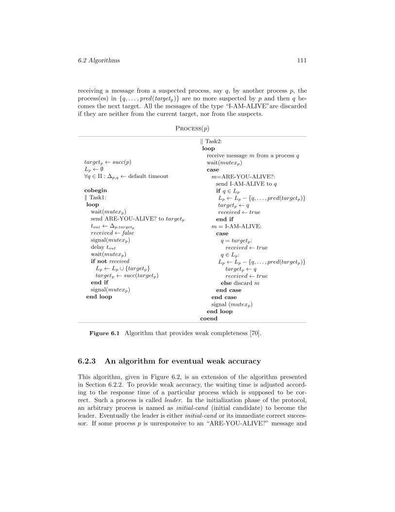
6.2 Algorithms 111
receiving a message from a suspected process, say q, by another process p, theprocess(es) in {q, . . . , pred(targetp)} are no more suspected by p and then q be-comes the next target. All the messages of the type “I-AM-ALIVE”are discardedif they are neither from the current target, nor from the suspects.
Process(p)
targetp ← succ(p)Lp ← ∅∀q ∈ Π : ∆p,q ← default timeout
cobegin‖ Task1:loop
wait(mutexp)send ARE-YOU-ALIVE? to targetptout ← ∆p,targetp
received← falsesignal(mutexp)delay toutwait(mutexp)if not receivedLp ← Lp ∪ {targetp}targetp ← succ(targetp)
end ifsignal(mutexp)
end loop
‖ Task2:loop
receive message m from a process qwait(mutexp)casem=ARE-YOU-ALIVE?:
send I-AM-ALIVE to qif q ∈ Lp
Lp ← Lp − {q, . . . , pred(targetp)}targetp ← qreceived← trueend if
m = I-AM-ALIVE:caseq = targetp:received← true
q ∈ Lp:Lp ← Lp − {q, . . . , pred(targetp)}
targetp ← qreceived← true
else discard mend case
end casesignal (mutexp)
end loopcoend
Figure 6.1 Algorithm that provides weak completeness [70].
6.2.3 An algorithm for eventual weak accuracy
This algorithm, given in Figure 6.2, is an extension of the algorithm presentedin Section 6.2.2. To provide weak accuracy, the waiting time is adjusted accord-ing to the response time of a particular process which is supposed to be cor-rect. Such a process is called leader. In the initialization phase of the protocol,an arbitrary process is named as initial-cand (initial candidate) to become theleader. Eventually the leader is either initial-cand or its immediate correct succes-sor. If some process p is unresponsive to an “ARE-YOU-ALIVE?” message and
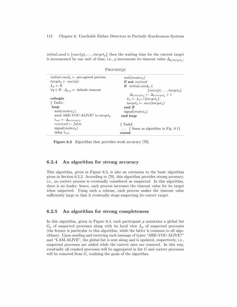
112 Chapter 6. Unreliable Failure Detectors in Partially Synchronous Systems
initial cand ∈ {succ(p), . . . , targetp} then the waiting time for the current targetis incremented by one unit of time, i.e., p increments its timeout value ∆p,targetp .
Process(p)
initial candp ← pre-agreed processtargetp ← succ(p)Lp ← ∅∀q ∈ Π : ∆p,q ← default timeout
cobegin‖ Task1:loop
wait(mutexp)send ARE-YOU-ALIVE? to targetptout ← ∆p,targetp
received← falsesignal(mutexp)delay tout
wait(mutexp)if not receivedif initial candp ∈
{succ(p), . . . , targetp}∆p,targetp ← ∆p,targetp + 1
Lp ← Lp ∪ {targetp}targetp ← succ(targetp)
end ifsignal(mutexp)
end loop
‖ Task2:. . . { Same as algorithm in Fig. 6.1}
coend
Figure 6.2 Algorithm that provides weak accuracy [70].
6.2.4 An algorithm for strong accuracy
This algorithm, given in Figure 6.3, is also an extension to the basic algorithmgiven in Section 6.2.2. According to [70], this algorithm provides strong accuracy,i.e., no correct process is eventually considered as suspected. In this algorithm,there is no leader; hence, each process increases the timeout value for its targetwhen suspected. Using such a scheme, each process makes the timeout valuesufficiently large so that it eventually stops suspecting its correct target.
6.2.5 An algorithm for strong completeness
In this algorithm, given in Figure 6.4, each participant p maintains a global listGp of suspected processes along with its local view Lp of suspected processes(the former is particular to this algorithm, while the latter is common to all algo-rithms). Upon sending and receiving each message of types “ARE-YOU-ALIVE?”and “I-AM-ALIVE”, the global list is sent along and is updated, respectively, i.e.,suspected processes are added while the correct ones are removed. In this way,eventually all crashed processes will be aggregated in list G and correct processeswill be removed from G, realizing the goals of the algorithm.
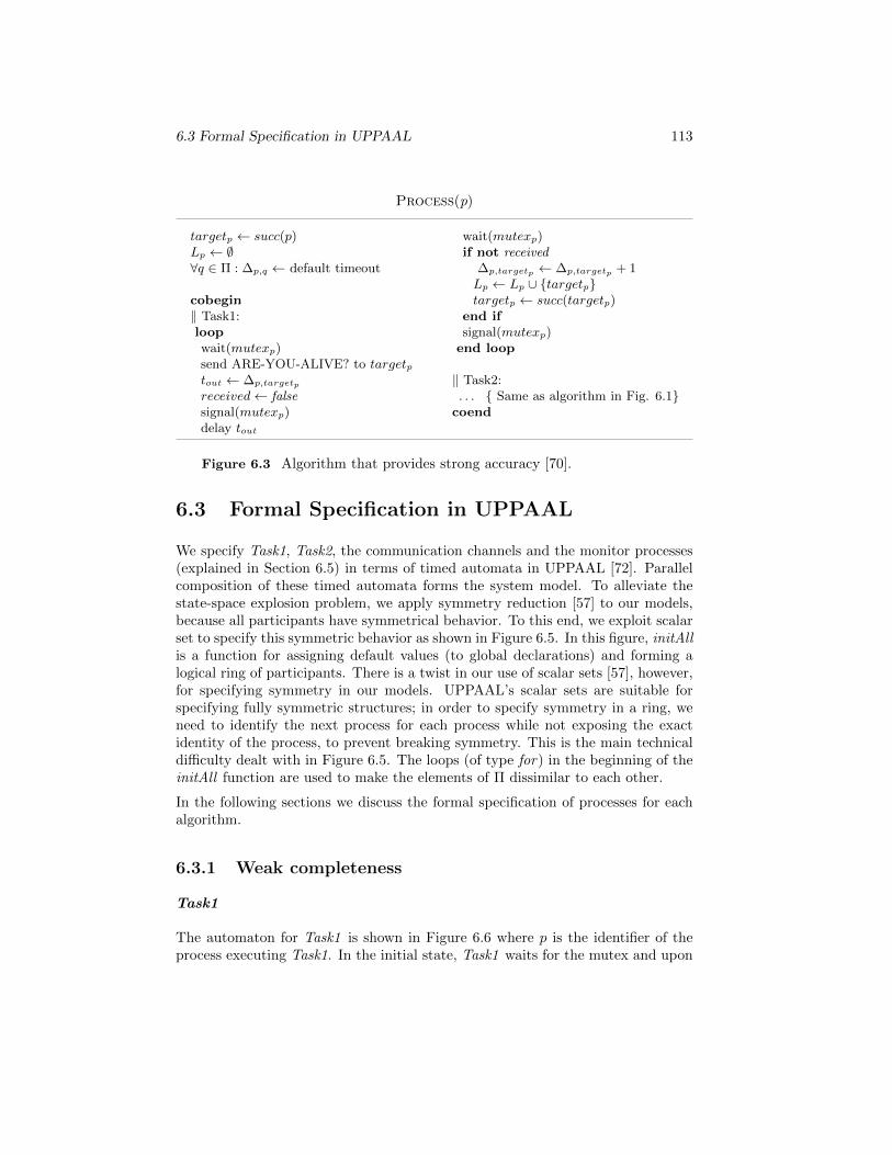
6.3 Formal Specification in UPPAAL 113
Process(p)
targetp ← succ(p)Lp ← ∅∀q ∈ Π : ∆p,q ← default timeout
cobegin‖ Task1:loopwait(mutexp)send ARE-YOU-ALIVE? to targetptout ← ∆p,targetp
received← falsesignal(mutexp)delay tout
wait(mutexp)if not received
∆p,targetp ← ∆p,targetp + 1Lp ← Lp ∪ {targetp}targetp ← succ(targetp)
end ifsignal(mutexp)end loop
‖ Task2:. . . { Same as algorithm in Fig. 6.1}
coend
Figure 6.3 Algorithm that provides strong accuracy [70].
6.3 Formal Specification in UPPAAL
We specify Task1, Task2, the communication channels and the monitor processes(explained in Section 6.5) in terms of timed automata in UPPAAL [72]. Parallelcomposition of these timed automata forms the system model. To alleviate thestate-space explosion problem, we apply symmetry reduction [57] to our models,because all participants have symmetrical behavior. To this end, we exploit scalarset to specify this symmetric behavior as shown in Figure 6.5. In this figure, initAllis a function for assigning default values (to global declarations) and forming alogical ring of participants. There is a twist in our use of scalar sets [57], however,for specifying symmetry in our models. UPPAAL’s scalar sets are suitable forspecifying fully symmetric structures; in order to specify symmetry in a ring, weneed to identify the next process for each process while not exposing the exactidentity of the process, to prevent breaking symmetry. This is the main technicaldifficulty dealt with in Figure 6.5. The loops (of type for) in the beginning of theinitAll function are used to make the elements of Π dissimilar to each other.
In the following sections we discuss the formal specification of processes for eachalgorithm.
6.3.1 Weak completeness
Task1
The automaton for Task1 is shown in Figure 6.6 where p is the identifier of theprocess executing Task1. In the initial state, Task1 waits for the mutex and upon
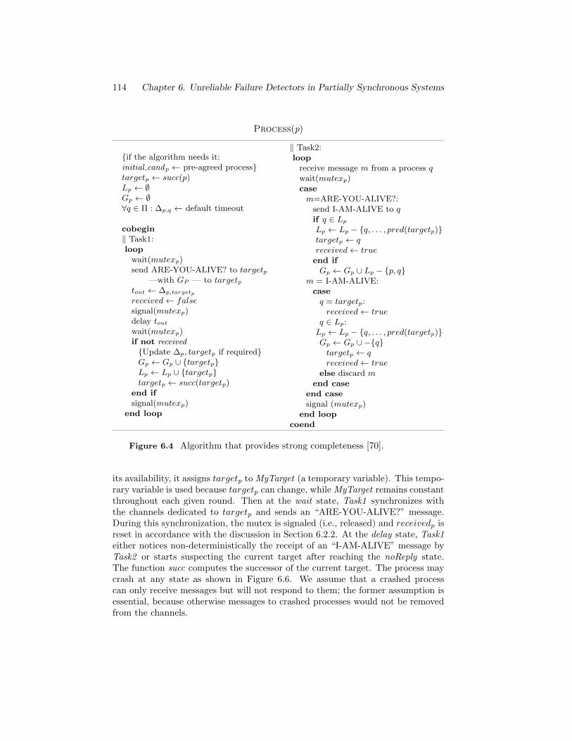
114 Chapter 6. Unreliable Failure Detectors in Partially Synchronous Systems
Process(p)
{if the algorithm needs it:initial candp ← pre-agreed process}targetp ← succ(p)Lp ← ∅Gp ← ∅∀q ∈ Π : ∆p,q ← default timeout
cobegin‖ Task1:loop
wait(mutexp)send ARE-YOU-ALIVE? to targetp
—with GP — to targetptout ← ∆p,targetp
received← falsesignal(mutexp)delay toutwait(mutexp)if not received{Update ∆p, targetp if required}Gp ← Gp ∪ {targetp}Lp ← Lp ∪ {targetp}targetp ← succ(targetp)
end ifsignal(mutexp)
end loop
‖ Task2:loop
receive message m from a process qwait(mutexp)casem=ARE-YOU-ALIVE?:
send I-AM-ALIVE to qif q ∈ Lp
Lp ← Lp − {q, . . . , pred(targetp)}targetp ← qreceived← trueend ifGp ← Gp ∪ Lp − {p, q}
m = I-AM-ALIVE:caseq = targetp:received← true
q ∈ Lp:Lp ← Lp − {q, . . . , pred(targetp)}Gp ← Gp ∪ −{q}targetp ← qreceived← true
else discard mend case
end casesignal (mutexp)
end loopcoend
Figure 6.4 Algorithm that provides strong completeness [70].
its availability, it assigns targetp to MyTarget (a temporary variable). This tempo-rary variable is used because targetp can change, while MyTarget remains constantthroughout each given round. Then at the wait state, Task1 synchronizes withthe channels dedicated to targetp and sends an “ARE-YOU-ALIVE?” message.During this synchronization, the mutex is signaled (i.e., released) and receivedp isreset in accordance with the discussion in Section 6.2.2. At the delay state, Task1either notices non-deterministically the receipt of an “I-AM-ALIVE” message byTask2 or starts suspecting the current target after reaching the noReply state.The function succ computes the successor of the current target. The process maycrash at any state as shown in Figure 6.6. We assume that a crashed processcan only receive messages but will not respond to them; the former assumption isessential, because otherwise messages to crashed processes would not be removedfrom the channels.
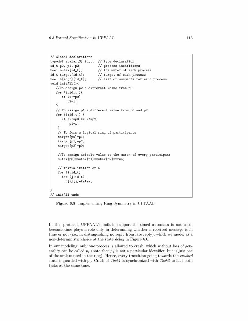
6.3 Formal Specification in UPPAAL 115
// Global declarations
typedef scalar[3] id_t; // type declaration
id_t p0, p1, p2; // process identifiers
bool mutex[id_t]; // the mutex of each process
id_t target[id_t]; // target of each process
bool L[id_t][id_t]; // list of suspects for each process
void initAll(){
//To assign p2 a different value from p0
for (i:id_t ){
if (i!=p0)
p2=i;
}
// To assign p1 a different value from p0 and p2
for (i:id_t ) {
if (i!=p0 && i!=p2)
p1=i;
}
// To form a logical ring of participants
target[p0]=p1;
target[p1]=p2;
target[p2]=p0;
//To assign default value to the mutex of every participant
mutex[p0]=mutex[p1]=mutex[p2]=true;
// initialization of L
for (i:id_t)
for (j:id_t)
L[i][j]=false;
}
// initAll ends
Figure 6.5 Implementing Ring Symmetry in UPPAAL
In this protocol, UPPAAL’s built-in support for timed automata is not used,because time plays a role only in determining whether a received message is intime or not (i.e., in distinguishing no reply from late reply), which we model as anon-deterministic choice at the state delay in Figure 6.6.
In our modeling, only one process is allowed to crash, which without loss of gen-erality can be called p1 (note that p1 is not a particular identifier, but is just oneof the scalars used in the ring). Hence, every transition going towards the crashedstate is guarded with p1. Crash of Task1 is synchronized with Task2 to halt bothtasks at the same time.
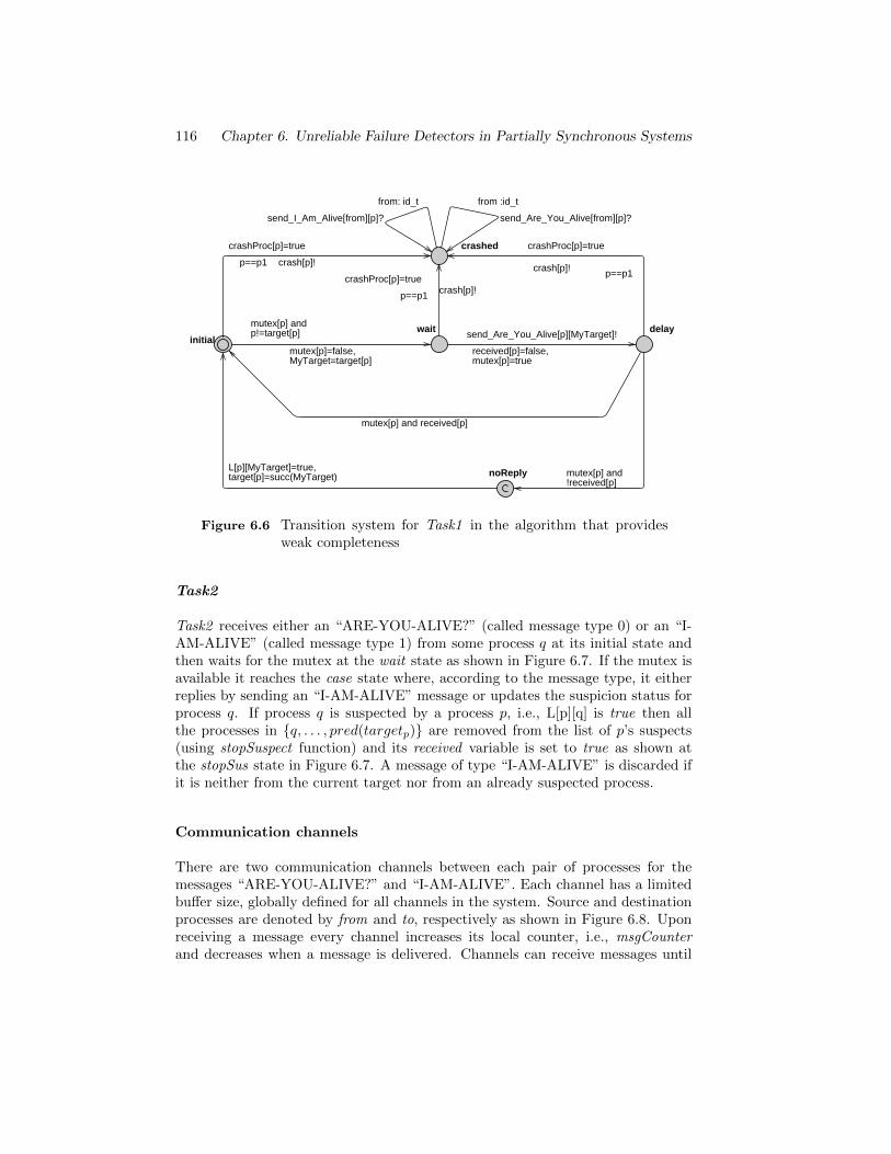
116 Chapter 6. Unreliable Failure Detectors in Partially Synchronous Systems
noReply
wait
crashed
delayinitial
from: id_t
send_I_Am_Alive[from][p]?
mutex[p] and p!=target[p]
mutex[p]=false,MyTarget=target[p]
from :id_t
send_Are_You_Alive[from][p]?
L[p][MyTarget]=true,target[p]=succ(MyTarget) mutex[p] and
!received[p]
p==p1 crash[p]!crashProc[p]=true
send_Are_You_Alive[p][MyTarget]!
received[p]=false,mutex[p]=true
mutex[p] and received[p]
p==p1crash[p]!
crashProc[p]=true
p==p1 crash[p]!
crashProc[p]=true
Figure 6.6 Transition system for Task1 in the algorithm that providesweak completeness
Task2
Task2 receives either an “ARE-YOU-ALIVE?” (called message type 0) or an “I-AM-ALIVE” (called message type 1) from some process q at its initial state andthen waits for the mutex at the wait state as shown in Figure 6.7. If the mutex isavailable it reaches the case state where, according to the message type, it eitherreplies by sending an “I-AM-ALIVE” message or updates the suspicion status forprocess q. If process q is suspected by a process p, i.e., L[p][q] is true then allthe processes in {q, . . . , pred(targetp)} are removed from the list of p’s suspects(using stopSuspect function) and its received variable is set to true as shown atthe stopSus state in Figure 6.7. A message of type “I-AM-ALIVE” is discarded ifit is neither from the current target nor from an already suspected process.
Communication channels
There are two communication channels between each pair of processes for themessages “ARE-YOU-ALIVE?” and “I-AM-ALIVE”. Each channel has a limitedbuffer size, globally defined for all channels in the system. Source and destinationprocesses are denoted by from and to, respectively as shown in Figure 6.8. Uponreceiving a message every channel increases its local counter, i.e., msgCounterand decreases when a message is delivered. Channels can receive messages until
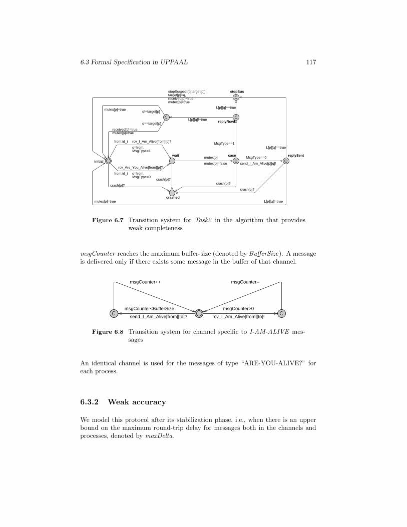
6.3 Formal Specification in UPPAAL 117
wait
stopSus
replyRcvd
replySentcase
crashed
initial
L[p][q]!=truemutex[p]=true
stopSuspect(q,target[p]),target[p]=q,received[p]=true,mutex[p]=true
q!=target[p]mutex[p]=true
q==target[p]
received[p]=true,mutex[p]=true
mutex[p]
mutex[p]=false
from:id_t rcv_I_Am_Alive[from][p]?
q=from,MsgType=1
L[p][q]==true
crash[p]?
L[p][q]!=true
crash[p]?
from:id_t
rcv_Are_You_Alive[from][p]?
q=from,MsgType=0
L[p][q]==true
crash[p]?
MsgType==1
MsgType==0
send_I_Am_Alive[p][q]!
crash[p]?
Figure 6.7 Transition system for Task2 in the algorithm that providesweak completeness
msgCounter reaches the maximum buffer-size (denoted by BufferSize). A messageis delivered only if there exists some message in the buffer of that channel.
msgCounter--
msgCounter>0
rcv_I_Am_Alive[from][to]!
msgCounter++
msgCounter<BufferSize
send_I_Am_Alive[from][to]?
Figure 6.8 Transition system for channel specific to I-AM-ALIVE mes-sages
An identical channel is used for the messages of type “ARE-YOU-ALIVE?” foreach process.
6.3.2 Weak accuracy
We model this protocol after its stabilization phase, i.e., when there is an upperbound on the maximum round-trip delay for messages both in the channels andprocesses, denoted by maxDelta.
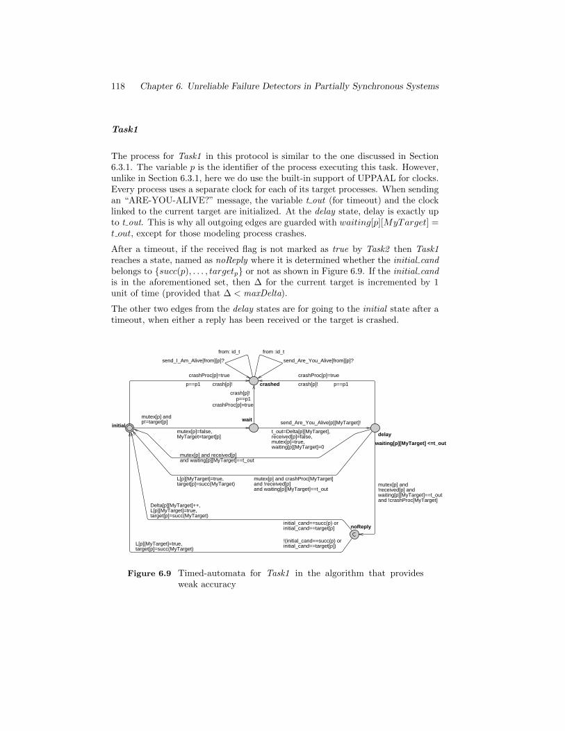
118 Chapter 6. Unreliable Failure Detectors in Partially Synchronous Systems
Task1
The process for Task1 in this protocol is similar to the one discussed in Section6.3.1. The variable p is the identifier of the process executing this task. However,unlike in Section 6.3.1, here we do use the built-in support of UPPAAL for clocks.Every process uses a separate clock for each of its target processes. When sendingan “ARE-YOU-ALIVE?” message, the variable t out (for timeout) and the clocklinked to the current target are initialized. At the delay state, delay is exactly upto t out. This is why all outgoing edges are guarded with waiting[p][MyTarget] =t out, except for those modeling process crashes.
After a timeout, if the received flag is not marked as true by Task2 then Task1reaches a state, named as noReply where it is determined whether the initial candbelongs to {succ(p), . . . , targetp} or not as shown in Figure 6.9. If the initial candis in the aforementioned set, then ∆ for the current target is incremented by 1unit of time (provided that ∆ < maxDelta).
The other two edges from the delay states are for going to the initial state after atimeout, when either a reply has been received or the target is crashed.
noReply
wait
crashed
delay
waiting[p][MyTarget] <=t_out
initial
from: id_t
send_I_Am_Alive[from][p]?
mutex[p] and p!=target[p]
mutex[p]=false,MyTarget=target[p]
mutex[p] and crashProc[MyTarget] and !received[p]and waiting[p][MyTarget]==t_out
L[p][MyTarget]=true,target[p]=succ(MyTarget)
from :id_t
send_Are_You_Alive[from][p]?
!(initial_cand==succ(p) orinitial_cand==target[p])L[p][MyTarget]=true,
target[p]=succ(MyTarget)
initial_cand==succ(p) orinitial_cand==target[p]
Delta[p][MyTarget]++,L[p][MyTarget]=true,target[p]=succ(MyTarget)
mutex[p] and !received[p] andwaiting[p][MyTarget]==t_outand !crashProc[MyTarget]
p==p1crash[p]!
crashProc[p]=true
send_Are_You_Alive[p][MyTarget]!
t_out=Delta[p][MyTarget],received[p]=false,mutex[p]=true,waiting[p][MyTarget]=0
mutex[p] and received[p]and waiting[p][MyTarget]==t_out
p==p1crash[p]!
crashProc[p]=true
p==p1 crash[p]!
crashProc[p]=true
Figure 6.9 Timed-automata for Task1 in the algorithm that providesweak accuracy
6.4 General Requirements 119
Task2
Task2 is exactly the same as the corresponding task discussed in Section 6.3.1except for the added invariant to make sure that the processing time remainswithin maxDelta. This invariant checks the amount of time spent for a receivedmessage so that in the remaining time (maximum delay=maxDelta) the receivedmessage is processed.
6.3.3 Strong accuracy
For this algorithm, Task1 discussed in Section 6.3.2 is slightly modified while Task2remains intact. The only difference is at the noReply state in Figure 6.9. Thereis only one outgoing transition from the noReply state to the initial state. Thistransition has no guard and updates ∆p,targetp , Lp and targetp as follows:
• ∆p,targetp = ∆p,targetp + 1,
• L[p][MyTarget] = true, and
• targetp = succ(MyTarget).
6.3.4 Strong completeness
In the specification of this protocol, we declare a global list G for all suspectedprocesses. Hence, Task1 of each process adds its target to G if the target issuspected and Task2 removes the process if a process from this list communicateswith its monitoring process. Task1 discussed in Section 6.3.3 is modified to addthe target in G to the only outgoing transition from the noReply state. There isno other change in Task1.
Task2 is also slightly modified by adding the list G, i.e., if an already suspectedprocess q sends an “I-AM-ALIVE” message to a process p, then p removes q fromG and likewise, if the received message is of the type “ARE-YOU-ALIVE?” thenboth p and q are removed from G.
6.4 General Requirements
The algorithms to implement unreliable failure detectors in partially synchronoussystems given in [70] are supposed to satisfy the following requirements.
1. Deadlock freedom: There must not be a deadlock in any protocol providedthat at least two processes are correct.
120 Chapter 6. Unreliable Failure Detectors in Partially Synchronous Systems
2. Weak completeness: For the protocol discussed in Section 6.2.2.
3. Eventual weak accuracy : For the protocol discussed in Section 6.2.3.
4. Strong accuracy : For the protocol discussed in Section 6.2.4.
5. Strong completeness: For the protocol discussed in Section 6.2.5.
6.5 Results
In this section, we report on our analysis results for all four algorithms presentedearlier in this chapter. For each algorithm, we first discuss the result of deadlockchecking in UPPAAL. In order to compare the effectiveness of UPPAAL, we com-pare its performance with two other model-checking tools, namely, FDR2 [88, 90]and mCRL2 [49]. Then, we propose a slight correction of the algorithms to removethe detected deadlock. Finally, we report on the verification of other propertieson the corrected algorithms.
6.5.1 Results for weak completeness
Detecting deadlocks in UPPAAL
In UPPAAL, we specify the absence of deadlock throughout the state space bythe following formula:
A[] not deadlock
We have used client and server components of UPPAAL 4.1.4 (64 bit, release July11, 2011) on different machines, i.e., a client on a Windows-based machine and theserver on a Unix-based server machine (4 × 2.5 Ghz processor and 64 GB RAM).
To express eventuality while not breaking symmetry, we devise monitor processesfor liveness properties, which we discuss in detail in the following sections. Inthe remainder of this section, we assume Π = {p0, p1, p2} and p0, p1, and p2,respectively, form a logical ring.
Figure 6.10 shows a counter-example where a finite buffer (of an arbitrary size)overflows and as a consequence the protocol encounters a deadlock. Particularly,the buffer used to store “ARE-YOU-ALIVE?” messages overflows due to sendingmore “ARE-YOU-ALIVE?” messages and receiving less “I-AM-ALIVE” messages.In this deadlock scenario, the process p2 sends “ARE-YOU-ALIVE?” to its targetp0 and after a timeout suspects p0. Then p2 receives “ARE-YOU-ALIVE?” fromp0, replies with “I-AM-ALIVE” and stops suspecting p0. Task2 of p2 receives“I-AM-ALIVE” but at that time the mutex is taken by Task1 which sends “ARE-YOU-ALIVE?” to p0 and releases the mutex. Task2 takes the mutex and processes
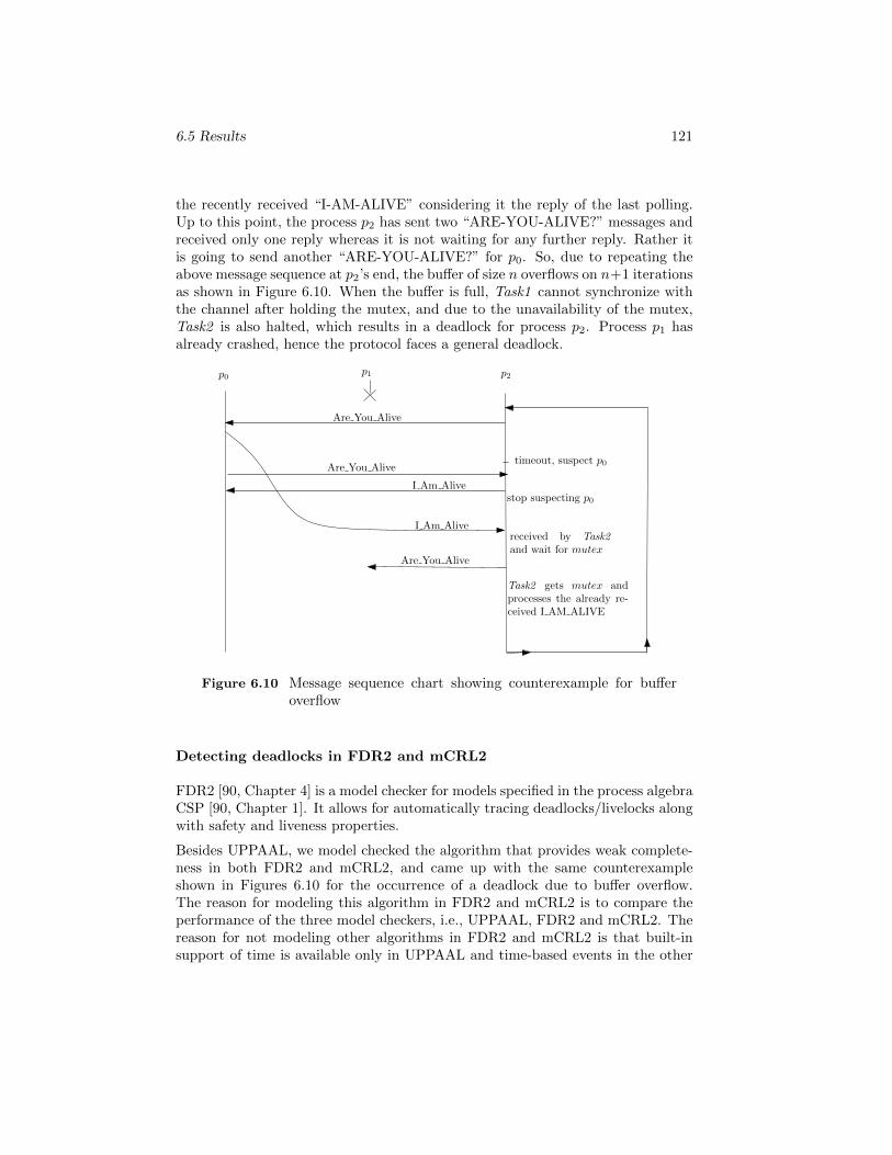
6.5 Results 121
the recently received “I-AM-ALIVE” considering it the reply of the last polling.Up to this point, the process p2 has sent two “ARE-YOU-ALIVE?” messages andreceived only one reply whereas it is not waiting for any further reply. Rather itis going to send another “ARE-YOU-ALIVE?” for p0. So, due to repeating theabove message sequence at p2’s end, the buffer of size n overflows on n+1 iterationsas shown in Figure 6.10. When the buffer is full, Task1 cannot synchronize withthe channel after holding the mutex, and due to the unavailability of the mutex,Task2 is also halted, which results in a deadlock for process p2. Process p1 hasalready crashed, hence the protocol faces a general deadlock.
p0 p1 p2
Are You Alive
timeout, suspect p0
stop suspecting p0
I Am Alive
Are You Alive
received by Task2and wait for mutex
Are You Alive
I Am Alive
Task2 gets mutex andprocesses the already re-ceived I AM ALIVE
Figure 6.10 Message sequence chart showing counterexample for bufferoverflow
Detecting deadlocks in FDR2 and mCRL2
FDR2 [90, Chapter 4] is a model checker for models specified in the process algebraCSP [90, Chapter 1]. It allows for automatically tracing deadlocks/livelocks alongwith safety and liveness properties.
Besides UPPAAL, we model checked the algorithm that provides weak complete-ness in both FDR2 and mCRL2, and came up with the same counterexampleshown in Figures 6.10 for the occurrence of a deadlock due to buffer overflow.The reason for modeling this algorithm in FDR2 and mCRL2 is to compare theperformance of the three model checkers, i.e., UPPAAL, FDR2 and mCRL2. Thereason for not modeling other algorithms in FDR2 and mCRL2 is that built-insupport of time is available only in UPPAAL and time-based events in the other
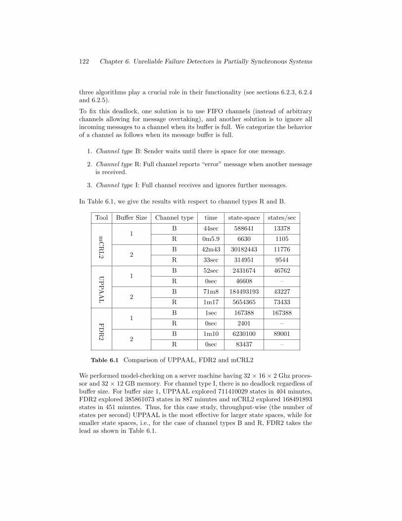
122 Chapter 6. Unreliable Failure Detectors in Partially Synchronous Systems
three algorithms play a crucial role in their functionality (see sections 6.2.3, 6.2.4and 6.2.5).
To fix this deadlock, one solution is to use FIFO channels (instead of arbitrarychannels allowing for message overtaking), and another solution is to ignore allincoming messages to a channel when its buffer is full. We categorize the behaviorof a channel as follows when its message buffer is full.
1. Channel type B: Sender waits until there is space for one message.
2. Channel type R: Full channel reports “error” message when another messageis received.
3. Channel type I: Full channel receives and ignores further messages.
In Table 6.1, we give the results with respect to channel types R and B.
Tool Buffer Size Channel type time state-space states/sec
mC
RL
2
1B 44sec 588641 13378
R 0m5.9 6630 1105
2B 42m43 30182443 11776
R 33sec 314951 9544
UP
PA
AL
1B 52sec 2431674 46762
R 0sec 46608 –
2B 71m8 184493193 43227
R 1m17 5654365 73433F
DR
2
1B 1sec 167388 167388
R 0sec 2401 –
2B 1m10 6230100 89001
R 0sec 83437 –
Table 6.1 Comparison of UPPAAL, FDR2 and mCRL2
We performed model-checking on a server machine having 32 × 16 × 2 Ghz proces-sor and 32 × 12 GB memory. For channel type I, there is no deadlock regardless ofbuffer size. For buffer size 1, UPPAAL explored 711410029 states in 404 minutes,FDR2 explored 385861073 states in 887 minutes and mCRL2 explored 168491893states in 451 minutes. Thus, for this case study, throughput-wise (the number ofstates per second) UPPAAL is the most effective for larger state spaces, while forsmaller state spaces, i.e., for the case of channel types B and R, FDR2 takes thelead as shown in Table 6.1.
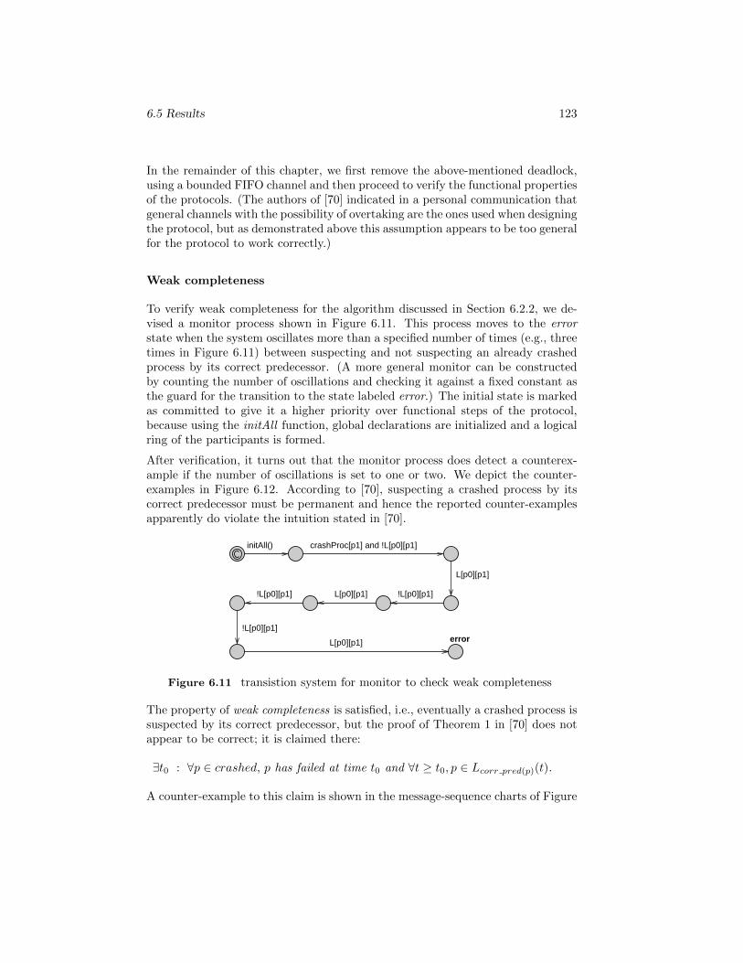
6.5 Results 123
In the remainder of this chapter, we first remove the above-mentioned deadlock,using a bounded FIFO channel and then proceed to verify the functional propertiesof the protocols. (The authors of [70] indicated in a personal communication thatgeneral channels with the possibility of overtaking are the ones used when designingthe protocol, but as demonstrated above this assumption appears to be too generalfor the protocol to work correctly.)
Weak completeness
To verify weak completeness for the algorithm discussed in Section 6.2.2, we de-vised a monitor process shown in Figure 6.11. This process moves to the errorstate when the system oscillates more than a specified number of times (e.g., threetimes in Figure 6.11) between suspecting and not suspecting an already crashedprocess by its correct predecessor. (A more general monitor can be constructedby counting the number of oscillations and checking it against a fixed constant asthe guard for the transition to the state labeled error.) The initial state is markedas committed to give it a higher priority over functional steps of the protocol,because using the initAll function, global declarations are initialized and a logicalring of the participants is formed.
After verification, it turns out that the monitor process does detect a counterex-ample if the number of oscillations is set to one or two. We depict the counter-examples in Figure 6.12. According to [70], suspecting a crashed process by itscorrect predecessor must be permanent and hence the reported counter-examplesapparently do violate the intuition stated in [70].
error
initAll()
!L[p0][p1]
L[p0][p1]
!L[p0][p1] L[p0][p1]
crashProc[p1] and !L[p0][p1]
!L[p0][p1]
L[p0][p1]
Figure 6.11 transistion system for monitor to check weak completeness
The property of weak completeness is satisfied, i.e., eventually a crashed process issuspected by its correct predecessor, but the proof of Theorem 1 in [70] does notappear to be correct; it is claimed there:
∃t0 : ∀p ∈ crashed, p has failed at time t0 and ∀t ≥ t0, p ∈ Lcorr pred(p)(t).
A counter-example to this claim is shown in the message-sequence charts of Figure
124 Chapter 6. Unreliable Failure Detectors in Partially Synchronous Systems
6.12, where (a) shows the scenario given as the proof of Theorem 1 while (b) and(c) depict the counterexamples to this proof, i.e., exclusion of a crashed processfrom the list of suspects. Although this exclusion is eventually stopped, oscillatingbetween suspecting and not-suspecting a crashed process is not addressed in theproof.
In Figure 6.12, a correct predecessor of a process p sends an “ARE-YOU-ALIVE?”message to p and receives its reply after which p crashes. At time t′, another “ARE-YOU-ALIVE?” message is sent and because of p’s crash failure, it is assumed thatthere will be no further message from p. Hence, p is permanently suspected asshown in Figure 6.12(a) after ∆correct pred(p),p(t′). However, Figure 6.12(b) showsreceiving of a “ARE-YOU-ALIVE?” message (late, due to unbounded delay inchannels) from p which causes it to stop suspecting process p. Figure 6.12(c)shows a different situation when Task2 of corr prd(p) receives a “I-AM-ALIVE”message and waits for the mutex but at the same time, timeout occurs at Task1which adds the process p in suspects and releases the mutex. Task2 takes themutex and processes the reply, due to which p is again excluded from the list ofsuspects.
6.5.2 Results for weak accuracy
Deadlock
The counterexample shown in Figure 6.13 exhibits the deadlock scenario which isdifferent from the one discussed in Section 6.5.1 but it resembles it in the sensethat it is also due to not-suspecting by receiving an “ARE-YOU-ALIVE?” messagewhen an “I-AM-ALIVE” message is expected. An explanation of reaching deadlockin process p0 is given below.
1. Send “ARE-YOU-ALIVE?” to p1, but p1 is already crashed.
2. Suspect p1 and change target to p2.
3. Send “ARE-YOU-ALIVE?” to p2.
4. Timeout and suspect p2.
5. Receive “ARE-YOU-ALIVE?” from p2.
6. Send “I-AM-ALIVE” and stop suspecting p2.
7. Send “ARE-YOU-ALIVE?” to p2.
8. Task2 receives “ARE-YOU-ALIVE?” from p2 and gets the mutex but cannotsend “I-AM-ALIVE” because the same message (mentioned at step 6) isalready there to be delivered. Now Task2 continues to wait for a free channel
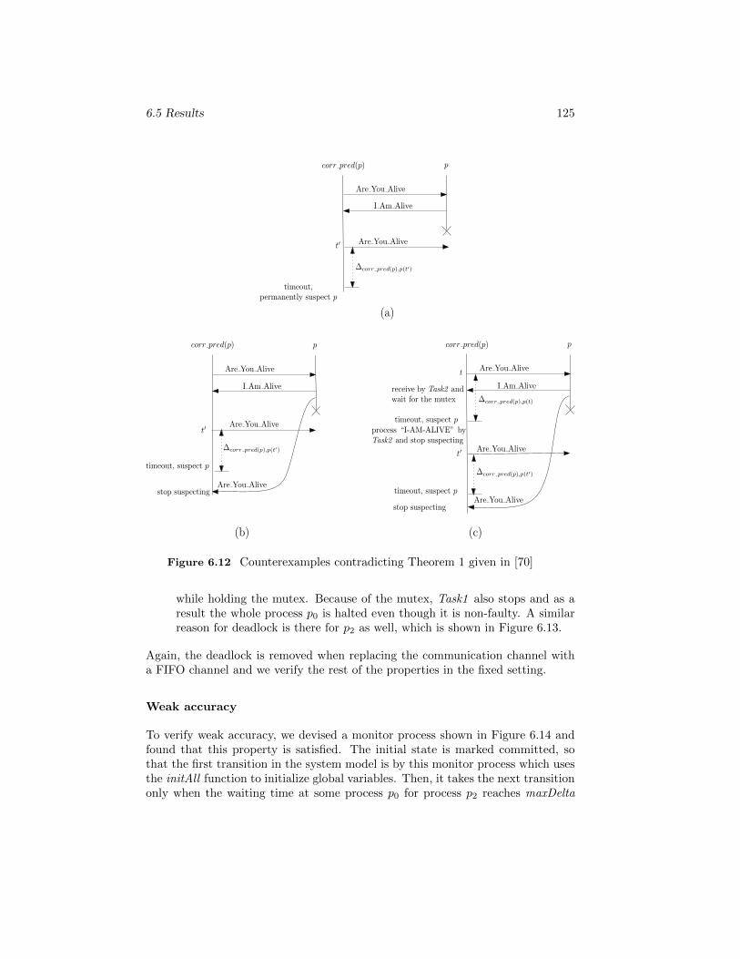
6.5 Results 125
corr pred(p) p
Are You Alive
stop suspecting
I Am Alive
Are You Alive
corr pred(p) p
Are You Alive
timeout, suspect p
I Am Alive
Are You Alive
Are You Alive
stop suspecting
corr pred(p) p
Are You Alive
timeout, suspect p
I Am Alive
Are You Alive
receive by Task2 andwait for the mutex
process “I-AM-ALIVE” byTask2 and stop suspecting
Are You Alivetimeout, suspect p
∆corr pred(p),p(t′)
∆corr pred(p),p(t′)
∆corr pred(p),p(t′)
timeout,permanently suspect p
t′
t′
t′
∆corr pred(p),p(t)
t
(a)
(b) (c)
Figure 6.12 Counterexamples contradicting Theorem 1 given in [70]
while holding the mutex. Because of the mutex, Task1 also stops and as aresult the whole process p0 is halted even though it is non-faulty. A similarreason for deadlock is there for p2 as well, which is shown in Figure 6.13.
Again, the deadlock is removed when replacing the communication channel witha FIFO channel and we verify the rest of the properties in the fixed setting.
Weak accuracy
To verify weak accuracy, we devised a monitor process shown in Figure 6.14 andfound that this property is satisfied. The initial state is marked committed, sothat the first transition in the system model is by this monitor process which usesthe initAll function to initialize global variables. Then, it takes the next transitiononly when the waiting time at some process p0 for process p2 reaches maxDelta
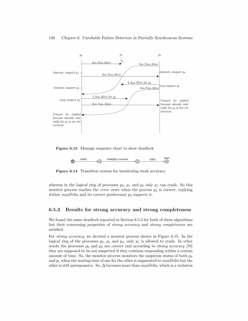
126 Chapter 6. Unreliable Failure Detectors in Partially Synchronous Systems
p0 p1 p2
Are You Alive
timeout, suspect p0
stop suspect p0
Are You Alive
Cannot be repliedbecause already sentreply for p0 is not yetreceived
Are You Alive
timeout, suspect p1
I Am Alive for p0
Are You Alive
I Am Alive for p2
Are You Alive
Cannot be repliedbecause already sentreply for p2 is not yetreceived
timeout, suspect p2
stop suspect p2
Figure 6.13 Message sequence chart to show deadlock
errorinitAll() L[a][c]Delta[a][c]==maxDelta
Figure 6.14 Transition system for monitoring weak accuracy
whereas in the logical ring of processes p0, p1 and p2 only p1 can crash. So thismonitor process reaches the error state when the process p2 is correct, replyingwithin maxDelta and its correct predecessor p0 suspects it.
6.5.3 Results for strong accuracy and strong completeness
We found the same deadlock reported in Section 6.5.2 for both of these algorithmsbut their concerning properties of strong accuracy and strong completeness aresatisfied.
For strong accuracy, we devised a monitor process shown in Figure 6.15. In thelogical ring of the processes p0, p1 and p2, only p1 is allowed to crash. In otherwords the processes p0 and p2 are correct and according to strong accuracy [70]they are supposed to be not suspected if they continue responding within a certainamount of time. So, the monitor process monitors the suspicion status of both p0
and p1 when the waiting time of one for the other is augmented to maxDelta but theother is still unresponsive. So, ∆ becomes more than maxDelta, which is a violation
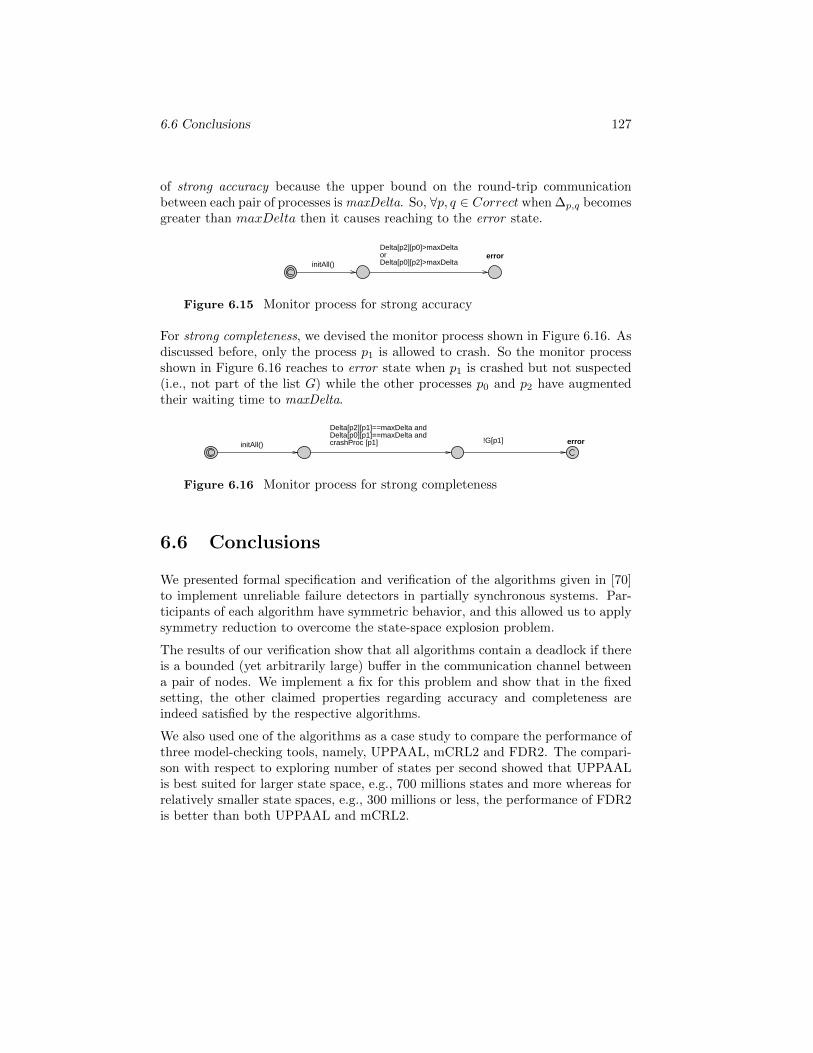
6.6 Conclusions 127
of strong accuracy because the upper bound on the round-trip communicationbetween each pair of processes is maxDelta. So, ∀p, q ∈ Correct when ∆p,q becomesgreater than maxDelta then it causes reaching to the error state.
errorDelta[p2][p0]>maxDeltaor Delta[p0][p2]>maxDeltainitAll()
Figure 6.15 Monitor process for strong accuracy
For strong completeness, we devised the monitor process shown in Figure 6.16. Asdiscussed before, only the process p1 is allowed to crash. So the monitor processshown in Figure 6.16 reaches to error state when p1 is crashed but not suspected(i.e., not part of the list G) while the other processes p0 and p2 have augmentedtheir waiting time to maxDelta.
errorinitAll() !G[p1]
Delta[p2][p1]==maxDelta andDelta[p0][p1]==maxDelta and crashProc [p1]
Figure 6.16 Monitor process for strong completeness
6.6 Conclusions
We presented formal specification and verification of the algorithms given in [70]to implement unreliable failure detectors in partially synchronous systems. Par-ticipants of each algorithm have symmetric behavior, and this allowed us to applysymmetry reduction to overcome the state-space explosion problem.
The results of our verification show that all algorithms contain a deadlock if thereis a bounded (yet arbitrarily large) buffer in the communication channel betweena pair of nodes. We implement a fix for this problem and show that in the fixedsetting, the other claimed properties regarding accuracy and completeness areindeed satisfied by the respective algorithms.
We also used one of the algorithms as a case study to compare the performance ofthree model-checking tools, namely, UPPAAL, mCRL2 and FDR2. The compari-son with respect to exploring number of states per second showed that UPPAALis best suited for larger state space, e.g., 700 millions states and more whereas forrelatively smaller state spaces, e.g., 300 millions or less, the performance of FDR2is better than both UPPAAL and mCRL2.

128 Chapter 6. Unreliable Failure Detectors in Partially Synchronous Systems
Chapter 7
Conclusions
130 Chapter 7 Conclusions
7.1 Introduction
In this chapter, we review the results achieved in this thesis. The research themeis mainly to investigate the application of prominent formal verification techniquesto failure-detection distributed algorithms where the system under considerationcan be synchronous, asynchronous or partially synchronous. Performing formalanalysis on distributed algorithms is still a challenge as the number of states growsexponentially with the number of concurrent/interactive system participants. Wefound that some papers claim to offer correct protocols while the details provided inthese papers are insufficient to establish those claims or even disprove the claimedproperties.
7.2 Achieved results
In Chapter 3, we found that the accelerated heartbeat protocols proposed by [47],violated some natural and essential properties. We proved the results by giv-ing counterexamples and developed the techniques to address the time-triggeredevents in mCRL2 and investigated the correct time bounds for all the protocolsdiscussed in [47] and [78]. In this chapter, we applied model checking as a debug-ging technique and found several issues in the verified protocols. Subsequently, weproposed some solutions to fix the discovered issues.
Chapter 4 shows the analysis of the consensus problem (a paradigm for reachingagreement despite failures) in an asynchronous system where the failure detectorsare unreliable (i.e., failure detectors may make mistakes). The problem we ana-lyzed, was first investigated in [21, 22]. According to [39], solving consensus inasynchronous systems is impossible even if:
• at most one process is allowed to crash, and
• all communication channels are reliable.
We proved the correctness of the proposed algorithms under its specified assump-tions.
In Chapter 5, we formally specified the group membership protocols proposed in[3]. We found that the protocol specifications and the text explaining the pro-tocols can be interpreted in different ways and even some natural interpretationscontradict each other. Our formalization with respect to different interpretationsshowed the violation of claimed properties. So to resolve the ambiguities and thedetected issues, we reconstructed the protocols and model-checked them.
Chapter 6 gave the results of performing formal analysis on the algorithms pro-posed by [70] for the purpose of implementing unreliable failure detectors in par-tially synchronous systems. We applied symmetry reduction techniques to manage
7.3 Future work 131
the state-space of this algorithm. We report that regardless of the buffer size, theprotocol is subject to buffer overflow. We propose fixes for avoiding this issue andmodel check the proposed algorithm in UPPAAL, FDR2 and mCRL2. We alsopresent a comparison of these three tools for model checking one of the given fourprotocols.
7.3 Future work
An interesting line of future research is to study the protocols discussed in thisthesis with respect to finite but arbitrarily many participants, i.e., performingparameterized model checking. Although the parameterized model checking prob-lem is undecidable in general [9], challenging future work is to establish sufficientconditions for yielding decidability such as proposed in [35].
In Chapter 3, we have investigated correct time bounds in which the given pro-tocols work correctly, i.e., time bounds for minimal tmin and tmax. tmin is theminimum waiting time and tmax is the maximum waiting time for each message inevery round (tmin is also the maximum-round trip delay of channels). Correctnessof the given protocols essentially depends upon the parameters for time boundsand hence by using parameterized model-checking with respect to tmin and tmax,we can prove the protocol correct for all possible values that have a certain ratio.HyTech [59] provides us with a means for such parametric analysis and we planto explore this in the future.
In Chapter 4, we performed formal analysis of two consensus protocols, where thecorrectness of the first one is proved with n − 1 rounds (where n is number ofparticipants) while in the second one we modeled three rounds. We modeled thefirst protocol as originally specified in [22] but for the second one, to avoid the statespace explosion problem, we fixed the round numbers. Future work with respect tothe second consensus algorithm is to study abstractions to relate different rounds,and hence to investigate this algorithm with unbounded round numbers such asthe formal analysis performed in [6].
In Chapter 5, we modeled the join protocol and applied the highway search tech-nique of [36] with restricted width and depth and found no violation of the prop-erties. In the future we would like to provide some quantitative measure of cor-rectness when applying highway search (e.g., the likelihood of finding a bug usingsome statistical measure on the explored state space).
In Chapter 6, we have found some action traces which shows the violation of somedesired properties but to overcome the state space explosion problem we applied afew restrictions like a restricted number of failures and a fixed number of rounds forprocesses believed to remain correct. Future work is to investigate the protocolswithout such limitations.

132 Chapter 7 Conclusions
References
[1] mcrl2 toolset. http://www.mcrl2.org.
[2] Rajeev Alur and David L. Dill. A theory of timed automata. Theor. Comput.Sci., 126(2):183–235, 1994.
[3] Yair Amir, Danny Dolev, Shlomo Kramer, and Dalia Malki. Membershipalgorithms for multicast communication groups. In WDAG ’92: Proceedingsof the 6th International Workshop on Distributed Algorithms, pages 292–312,London, UK, 1992. Springer-Verlag.
[4] Yair Amir, Danny Dolev, Shlomo Kramer, and Dalia Malki. Membership al-gorithms in broadcast domains. Technical Report 10, The Hebrew Universityof Jerusalem, 1992.
[5] Yair Amir, Danny Dolev, Shlomo Kramer, and Dalia Malki. Transis: Acommunication subsystem for high availability. In FTCS, pages 76–84, 1992.
[6] Xin An and Jun Pang. Model checking round-based distributed algorithms.In Radu Calinescu, Richard F. Paige, and Marta Z. Kwiatkowska, editors,ICECCS, pages 127–135. IEEE Computer Society, 2010.
[7] Emmanuelle Anceaume, Bernadette Charron-bost, Pascale Minet, and SamToueg. On the formal specification of group membership services. TechnicalReport 95-1534, Department of Computer Science, Cornell University, 1995.
[8] David P. Anderson. BOINC: A system for public-resource computing andstorage. In 5th IEEE/ACM International Workshop on Grid Computing,pages 4–10, Washington, DC, USA, 2004. IEEE Computer Society.
[9] Krzysztof R. Apt and Dexter Kozen. Limits for automatic verification offinite-state concurrent systems. Inf. Process. Lett., 22(6):307–309, 1986.
[10] Muhammad Atif. Analysis and verification of two-phase commit & three-phase commit protocols. In Proceedings of the 5th International Conferenceon Emerging Technologies, ICET 2009, pages 326 –331. IEEE, 2009.
133
134 References
[11] Muhammad Atif. Formal analysis of consensus protocols in asynchronousdistributed systems. Technical Report CSR-09-16, Department of ComputerScience, Eindhoven University of Technology, Eindhoven, The Netherlands,2009.
[12] Muhammad Atif, Sjoerd Cranen, and MohammadReza Mousavi. Recon-struction and verification of group membership protocols. Technical ReportCSR-10-08, Department of Computer Science, Eindhoven University of Tech-nology, Eindhoven, The Netherlands, 2010.
[13] Muhammad Atif and MohammadReza Mousavi. Formal specification andanalysis of accelerated heartbeat protocols. Technical Report CSR-09-04,Department of Computer Science, Eindhoven University of Technology,Eindhoven, The Netherlands, 2009.
[14] Muhammad Atif, MohammadReza Mousavi, and Ammar Osaiweran. Formalverification of unreliable failure detectors in partially synchronous systems.Technical Report CSR-11-12, Department of Computer Science, EindhovenUniversity of Technology, Eindhoven, The Netherlands, 2011.
[15] Hagit Attiya and Jennifer Welch. Distributed Computing: Fundamentals,Simulations, and Advanced Topics. Wiley-Interscience, 2004.
[16] Ozalp Babaoglu, Renzo Davoli, and Alberto Montresor. Group communi-cation in partitionable systems: Specification and algorithms. IEEE Trans.Software Eng., 27(4):308–336, 2001.
[17] Jos C. M. Baeten and W. Peter Weijland. Process Algebra. CambridgeUniversity Press, New York, NY, USA, 1990.
[18] Gerd Behrmann, Alexandre David, and Kim G. Larsen. A tutorial on UP-PAAL. In Marco Bernardo and Flavio Corradini, editors, SFM, volume 3185of Lecture Notes in Computer Science, pages 200–236. Springer, 2004.
[19] Bard Bloom. Constructing two-writer atomic registers. IEEE Transactionson Computers, 37(12):1506–1514, 1988.
[20] Ed Brinksma, Rance Cleaveland, Kim G. Larsen, Tiziana Margaria, andBernhard Steffen, editors. Tools and Algorithms for Construction and Anal-ysis of Systems, First International Workshop, TACAS ’95, Aarhus, Den-mark, May 19-20, 1995, Proceedings, volume 1019 of Lecture Notes in Com-puter Science. Springer, 1995.
[21] Tushar Deepak Chandra, Vassos Hadzilacos, and Sam Toueg. The weakestfailure detector for solving consensus. In Proceedings of the eleventh annualACM symposium on Principles of distributed computing, PODC ’92, pages147–158, New York, NY, USA, 1992. ACM.
References 135
[22] Tushar Deepak Chandra and Sam Toueg. Unreliable failure detectors forreliable distributed systems. J. ACM, 43(2):225–267, 1996.
[23] Daniel Marcos Chapiro. Globally-asynchronous locally-synchronous systems(performance, reliability, digital). PhD thesis, Stanford, CA, USA, 1985.
[24] Bernadette Charron-Bost, Martin Hutle, and Josef Widder. In search of losttime. Inf. Process. Lett., 110(21):928–933, 2010.
[25] Bernadette Charron-Bost and Andre Schiper. The Heard-Of model: Uni-fying all benign failures. Technical Report LSR-REPORT-2006-004, Ecolepolytechnique federale de Lausanne (EPFL), 2006.
[26] Bernadette Charron-Bost and Andre Schiper. Improving Fast Paxos: beingoptimistic with no overhead. In Proceedings of the 12th IEEE Pacific RimInternational Symposium on Dependable Computing (PRDC 2006), pages287–295. IEEE Computer Society, 2006.
[27] Bernadette Charron-Bost and Andre Schiper. The Heard-Of model: com-puting in distributed systems with benign faults. Distributed Computing,22(1):49–71, 2009.
[28] Gregory V. Chockler, Idit Keidar, and Roman Vitenberg. Group communica-tion specifications: a comprehensive study. ACM Comput. Surv., 33(4):427–469, 2001.
[29] Sjoerd Cranen, Jan Friso Groote, and Michel A. Reniers. A linear translationfrom LTL to the first-order modal µ-calculus. Technical Report CSR-10-09, Department of Computer Science, Eindhoven University of Technology,Eindhoven, The Netherlands, 2010.
[30] Flaviu Cristian. Synchronous and asynchronous group communication. Com-mun. ACM, 39:88–97, 1996.
[31] Edsger W. Dijkstra. Solution of a problem in concurrent programming con-trol. Commun. ACM, 8:569, 1965.
[32] Danny Dolev, Cynthia Dwork, and Larry Stockmeyer. On the minimal syn-chronism needed for distributed consensus. J. ACM, 34:77–97, January 1987.
[33] Danny Dolev and H. Raymond Strong. Authenticated algorithms for byzan-tine agreement. SIAM J. Comput., 12(4):656–666, 1983.
[34] Assia Doudou, Benoıt Garbinato, and Rachid Guerraoui. Encapsulatingfailure detection: From crash to byzantine failures. In Johann Blieberger andAlfred Strohmeier, editors, Proceedings of the 7th International Conferenceon Reliable Software Technologies - Ada-Europe 2002, volume 2361 of LectureNotes in Computer Science, pages 24–50. Springer, 2002.
136 References
[35] E. Allen Emerson and Vineet Kahlon. Parameterized model checking ofring-based message passing systems. In Jerzy Marcinkowski and AndrzejTarlecki, editors, CSL, volume 3210 of Lecture Notes in Computer Science,pages 325–339. Springer, 2004.
[36] Tom A.N. Engels, Jan Friso Groote, Muck J. van Weerdenburg, andTim A.C. Willemse. Search algorithms for automated validation. Journal ofLogic and Algebraic Programming, 78(4):274 – 287, 2009.
[37] Jean-Claude Fernandez, Hubert Garavel, Alain Kerbrat, Laurent Mounier,Radu Mateescu, and Mihaela Sighireanu. Cadp - a protocol validation andverification toolbox. In CAV, pages 437–440, 1996.
[38] Faith Fich and Eric Ruppert. Hundreds of impossibility results for dis-tributed computing. Distributed Computing, 16:121–163, 2003.
[39] Michael J. Fischer. The consensus problem in unreliable distributed systems(a brief survey). In Marek Karpinski, editor, FCT, volume 158 of LectureNotes in Computer Science, pages 127–140. Springer, 1983.
[40] Michael J. Fischer, Nancy A. Lynch, and Michael S. Paterson. Impossibilityof distributed consensus with one faulty process. J. ACM, 32:374–382, 1985.
[41] Wan Fokkink, Jan Friso Groote, Jun Pang, Bahareh Badban, and Jacovan de Pol. Verifying a sliding window protocol in µCRL. In Charles Rat-tray, Savi Maharaj, and Carron Shankland, editors, Algebraic Methodologyand Software Technology, volume 3116 of Lecture Notes in Computer Sci-ence, pages 148–163. Springer, 2004.
[42] Wan Fokkink, Allard Kakebeen, and Jun Pang. Adapting the UPPAALmodel of a distributed lift system. In Farhad Arbab and Marjan Sirjani,editors, Fundamentals of Software Engineering, volume 4767 of Lecture Notesin Computer Science, pages 81–97. Springer, 2007.
[43] Rachele Fuzzati, Massimo Merro, and Uwe Nestmann. Distributed consen-sus, revisited. Acta Inf., 44(6):377–425, 2007.
[44] Hubert Garavel, Frederic Lang, Radu Mateescu, and Wendelin Serwe.CADP 2006: A Toolbox for the Construction and Analysis of DistributedProcesses. In Werner Damm and Holger Hermanns, editors, Computer AidedVerification (CAV’2007) Lecture Notes in Computer Science, volume 4590 ofLecture Notes in Computer Science, pages 158–163, Berlin Germany, 2007.
[45] Hubert Garavel, Radu Mateescu, Frederic Lang, and Wendelin Serwe. CADP2006: A toolbox for the construction and analysis of distributed processes.volume 4590 of Lecture Notes in Computer Science, pages 158–163. Springer,2007.
References 137
[46] Biniam Gebremichael, Frits Vaandrager, and Miaomiao Zhang. Analysis ofthe zeroconf protocol using UPPAAL. In EMSOFT ’06: Proceedings of the6th ACM & IEEE International conference on Embedded software, pages242–251, New York, NY, USA, 2006. ACM.
[47] Mohamed G. Gouda and Tommy M. McGuire. Accelerated heartbeat pro-tocols. In ICDCS, pages 202–209, 1998.
[48] Mohamed G. Gouda and Tommy M. McGuire. Alert communication primi-tives above tcp. J. High Speed Netw., 9(2):139–150, 2000.
[49] Jan Friso Groote, Aad Mathijssen, Michel A. Reniers, Yaroslav S. Usenko,and Muck van Weerdenburg. Analysis of distributed systems with mCRL2.In Handbook of Process Algebra for Parallel and Distributed Processing, pages99–128. CRC Press, 2009.
[50] Jan Friso Groote, Aad Mathijssen, Muck van Weerdenburg, and Yaroslav S.Usenko. From µCRL to mCRL2: motivation and outline. Electr. NotesTheor. Comput. Sci., 162:191–196, 2006.
[51] Jan Friso Groote, Jun Pang, and Arno G. Wouters. Analysis of a distributedsystem for lifting trucks. J. Log. Algebr. Program., 55(1-2):21–56, 2003.
[52] Jan Friso Groote, Alban Ponse, and Yaroslav S. Usenko. Linearization inparallel pCRL. J. Log. Algebr. Program., 48(1-2):39–70, 2001.
[53] Jan Friso Groote and Michel Reniers. Modelling and analysis of communi-cating systems. preprint (2010), available at www.win.tue.nl/~jfg/educ/
2IW26/herfst2010/mcrl2-book.pdf.
[54] Jan Friso Groote and Frank van Ham. Large state space visualization. InHubert Garavel and John Hatcliff, editors, TACAS, volume 2619 of LectureNotes in Computer Science, pages 585–590. Springer, 2003.
[55] Jan Friso Groote and Tim A. C. Willemse. Model-checking processes withdata. Sci. Comput. Program., 56(3):251–273, 2005.
[56] Vassos Hadzilacos and Joseph Y. Halpern. Message-optimal protocols forbyzantine agreement (extended abstract). In Proceedings of the tenth annualACM symposium on Principles of distributed computing, PODC ’91, pages309–323, New York, NY, USA, 1991. ACM.
[57] Martijn Hendriks, Gerd Behrmann, Kim G. Larsen, Peter Niebert, andFrits W. Vaandrager. Adding symmetry reduction to UPPAAL. In Kim G.Larsen and Peter Niebert, editors, Formal Modeling and Analysis of TimedSystems, volume 2791 of Lecture Notes in Computer Science, pages 46–59.Springer, 2003.
138 References
[58] Matthew Hennessy and Robin Milner. Algebraic laws for nondeterminismand concurrency. J. ACM, 32(1):137–161, 1985.
[59] Thomas A. Henzinger, Pei-Hsin Ho, and Howard Wong-Toi. A user guide tohytech. In Brinksma et al. [20], pages 41–71.
[60] Maurice Herlihy and Nir Shavit. The art of multiprocessor programming.Morgan Kaufmann, 2008.
[61] Hugh W. Holbrook, Sandeep K. Singhal, and David R. Cheriton. Log-basedreceiver-reliable multicast for distributed interactive simulation. SIGCOMMComput. Commun. Rev., 25(4):328–341, 1995.
[62] Kim Potter Kihlstrom, Louise E. Moser, and P. M. Melliar-Smith. Byzantinefault detectors for solving consensus. Comput. J., 46(1):16–35, 2003.
[63] Dexter Kozen. Results on the propositional mu-calculus. Theor. Comput.Sci., 27:333–354, 1983.
[64] Ajay D. Kshemkalyani and Mukesh Singhal. Distributed Computing. Cam-bridge University Press, 2008.
[65] Leslie Lamport. Time, clocks, and the ordering of events in a distributedsystem. Commun. ACM, 21(7):558–565, 1978.
[66] Leslie Lamport. On interprocess communication. part i: Basic formalism.Distributed Computing, 1(2):77–85, 1986.
[67] Leslie Lamport. On interprocess communication. part ii: Algorithms. Dis-tributed Computing, 1(2):86–101, 1986.
[68] Leslie Lamport. The part-time parliament. ACM Trans. Comput. Syst.,16(2):133–169, 1998.
[69] Leslie Lamport, Robert E. Shostak, and Marshall C. Pease. The byzantinegenerals problem. ACM Trans. Program. Lang. Syst., 4(3):382–401, 1982.
[70] Mikel Larrea, Sergio Arevalo, and Antonio Fernandez. Efficient algorithmsto implement unreliable failure detectors in partially synchronous systems.In Prasad Jayanti, editor, DISC, volume 1693 of Lecture Notes in ComputerScience, pages 34–48. Springer, 1999.
[71] Kim G. Larsen, Paul Pettersson, and Wang Yi. Model-checking for real-timesystems. In Horst Reichel, editor, International Symposium on Fundamentalsof Computation Theory, volume 965 of Lecture Notes in Computer Science,pages 62–88. Springer, 1995.
[72] Kim G. Larsen, Paul Pettersson, and Wang Yi. UPPAAL in a nutshell.STTT, 1(1-2):134–152, 1997.
References 139
[73] Nancy Lynch. A hundred impossibility proofs for distributed computing.In Proceedings of the eighth annual ACM Symposium on Principles of dis-tributed computing, pages 1–28, New York, NY, USA, 1989. ACM.
[74] Nancy A. Lynch. Distributed Algorithms. Morgan Kaufmann PublishersInc., San Francisco, CA, USA, 1996.
[75] Angelika Mader. Modal µ-calculus, model checking and gauß elimination.In Brinksma et al. [20], pages 72–88.
[76] Dahlia Malkhi and Michael K. Reiter. Unreliable intrusion detection in dis-tributed computations. In Proceedings of the 10th Computer Security Foun-dations Workshop (CSFW ’97), pages 116–125. IEEE Computer Society,1997.
[77] Kirk Martinez, Paritosh Padhy, Ahmed Elsaify, Gang Zou, A. Riddoch,Jane K. Hart, and H. L. R. Ong. Deploying a sensor network in an ex-treme environment. In Proceedings of the IEEE International Conference onSensor Networks, Ubiquitous, and Trustworthy Computing, pages 186–193.IEEE Computer Society, 2006.
[78] Tommy M. McGuire and Mohamed G. Gouda. The Austin Protocol Compiler(Advances in Information Security). Springer-Verlag TELOS, Santa Clara,CA, USA, 2004.
[79] Sape Mullender, editor. Distributed systems. ACM, New York, NY, USA,1989.
[80] Gil Neiger and Sam Toueg. Automatically increasing the fault-tolerance ofdistributed algorithms. J. Algorithms, 11(3):374–419, 1990.
[81] Uwe Nestmann, Rachele Fuzzati, and Massimo Merro. Modeling consensusin a process calculus. In Roberto M. Amadio and Denis Lugiez, editors,Proceedings of the 14th International Conference on Concurrency Theory(CONCUR 2003), volume 2761 of Lecture Notes in Computer Science, pages393–407. Springer-Verlag, 2003.
[82] Marshall C. Pease, Robert E. Shostak, and Leslie Lamport. Reaching agree-ment in the presence of faults. J. ACM, 27(2):228–234, 1980.
[83] Kenneth J. Perry and Sam Toueg. Distributed agreement in the presence ofprocessor and communication faults. IEEE Trans. Software Eng., 12(3):477–482, 1986.
[84] Amir Pnueli. The temporal logic of programs. In Foundations of ComputerScience, pages 46–57. IEEE, 1977.
140 References
[85] John H. Reif. Synthesis of parallel algorithms. Morgan Kaufmann, SantaMateo, California, USA, 1993.
[86] Aleta Ricciardi. The Group Membership Problem in Asynchronous Systems.PhD thesis, Department of Computer Science, Cornell University, 1993.
[87] Dirk Riehle. How and why Wikipedia works: an interview with AngelaBeesley, Elisabeth Bauer, and Kizu Naoko. In Proceedings of the 2006 In-ternational Symposium on Wikis, pages 3–8, New York, NY, USA, 2006.ACM.
[88] Bill Roscoe. Understanding Concurrent Systems. Springer, 2010.
[89] Valerio Rosset, Pedro F. Souto, and Francisco Vasques. Formal verificationof a group membership protocol using model checking. In Robert Meersmanand Zahir Tari, editors, On The Move, volume 4803 of Lecture Notes inComputer Science, pages 471–488. Springer, 2007.
[90] Peter Y. A. Ryan and Steve A. Schneider. The modelling and analysis ofsecurity protocols: the CSP approach. Addison-Wesley Professional, firstedition, 2000.
[91] Nicola Santoro. Design and Analysis of Distributed Algorithms (Wiley Serieson Parallel and Distributed Computing). Wiley-Interscience, 2006.
[92] Andre Schiper, Kenneth Birman, and Pat Stephenson. Lightweight causaland atomic group multicast. ACM Transactions on Computer Systems(TOCS), 9(3):314, 1991.
[93] Fred B. Schneider. Byzantine generals in action: Implementing fail-stopprocessors. ACM Trans. Comput. Syst., 2(2):145–154, 1984.
[94] Andrew S. Tanenbaum and Maarten Van Steen. Distributed Systems: Prin-ciples and Paradigms. Prentice Hall, 2006.
[95] Yung Ting, F. M. Shan, Wen-Bin Lu, and Cheng-Hung Chen. Implemen-tation and evaluation of failsafe computer-controlled systems. Comput. Ind.Eng., 42(2-4):401–415, 2002.
[96] Tatsuhiro Tsuchiya and Andre Schiper. Using bounded model checking toverify consensus algorithms. In Gadi Taubenfeld, editor, 22nd InternationalSymposium on Distributed Computing (DISC’ 2008), volume 5218 of LectureNotes in Computer Science, pages 466–480. Springer, 2008.
[97] Tatsuhiro Tsuchiya and Andre Schiper. Verification of consensus algorithmsusing satisfiability solving. Distributed Computing, 23(5-6):341–358, 2011.
References 141
[98] Jaco van de Pol. Jitty: A rewriter with strategy annotations. In SophieTison, editor, RTA, volume 2378 of Lecture Notes in Computer Science,pages 367–370. Springer, 2002.
[99] Jaco van de Pol and Miguel Valero Espada. Verification of javaspacestm
parallel programs. In Application of Concurrency to System Design, pages196–205. IEEE Computer Society, 2003.
[100] Werner Vogels. World wide failures. In Andrew Herbert and Andrew S.Tanenbaum, editors, ACM SIGOPS European Workshop, pages 115–120.ACM, 1996.
[101] Guojun Wang, Zhongshan Gao, Lifan Zhang, and Jiannong Cao. Prediction-based multicast mobility management in mobile internet. In Yi Pan, DaoxuChen, Minyi Guo, Jiannong Cao, and Jack Dongarra, editors, InternationalSymposium on Parallel and Distributed Processing with Applications, volume3758 of Lecture Notes in Computer Science, pages 1024–1035. Springer, 2005.
[102] Sergio Yovine. Model checking timed automata. In Grzegorz Rozenberg andFrits W. Vaandrager, editors, European Educational Forum: School on Em-bedded Systems, volume 1494 of Lecture Notes in Computer Science, pages114–152. Springer, 1996.

142 References
Appendix A
mCRL2 Specifications forHeartbeat Protocols
143
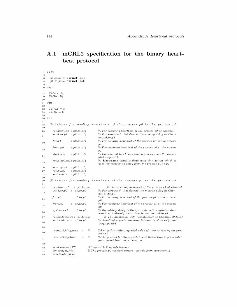
144 Appendix A. Heartbeat protocols
A.1 mCRL2 specification for the binary heart-beat protocol
1 sort2
3 p0 to p1 = struct hb0;4 p1 to p0 = struct hb1;5
6 map7
8 TMAX : N;9 TMIN : N;
10
11 eqn12
13 TMAX = 6;14 TMIN = 1;15
16 act17
18 % Actions for sending hear tbea t s of the process p0 to the process p119
20 rcv from p0 : p0 to p1 ; % For receiving heartbeat of the process p0 at channel
21send to p1 : p0 to p1 ; % For stopwatch that detects the messag delay in Chan-
nel p0 to p1
22for p1 : p0 to p1 ; % For sending heartbeat of the process p0 to the process
p1
23from p0 : p0 to p1 ; % For receiving heartbeat of the process p0 at the process
p1
24start sw4 : p0 to p1 ; % Channel p0 to p1 uses this action to start the associ-
ated stopwatch
25rcv start sw4 : p0 to p1 ; % Staopwatch starts ticking with this action which is
used for measuring delay from the process p0 to p1
26 sent by p0 : p0 to p1 ;
27 rcv by p1 : p0 to p1 ;
28 sw4 starts : p0 to p1 ;29
30 % Actions for sending hear tbea t s of the process p1 to the process p031
32 rcv from p1 : p1 to p0 ; % For receiving heartbeat of the process p1 at channel
33send to p0 : p1 to p0 ; % For stopwatch that detects the messag delay in Chan-
nel p1 to p0
34for p0 : p1 to p0 ; % For sending heartbeat of the process p1 to the process
p0
35from p1 : p1 to p0 ; % For receiving heartbeat of the process p1 at the process
p0
36update sw4 : p1 to p0 ; % Round-trip delay is fixed, so this action updates stop-
watch with already spent time in channel p0 to p1
37 rcv update sw4 : p1 to p0 ; % To synchronize with ‘update sw4’ at Channel p0 to p1
38sw4 updated : p1 to p0 ; % Result of scynchronixation between ‘update sw4’ and
‘sw4 updated’
39
40send ticking time : N; %Using this action, updated value of tmax is sent by the pro-
cess p0
41rcv ticking time : N; %The process fpr stopewatch 2 uses this action to get a value
for timeout from the process p0
42
43 send timeout P0 ; %Stopwatch 2 signals timeout
44 timeout at P0 ; %The process p0 receives timeout signals from stopwatch 2
45 inactivate p0 nv ;
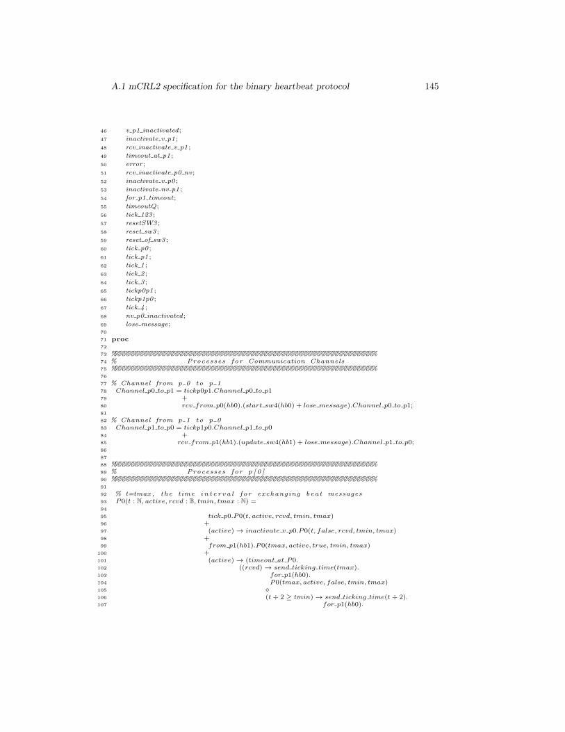
A.1 mCRL2 specification for the binary heartbeat protocol 145
46 v p1 inactivated;
47 inactivate v p1 ;
48 rcv inactivate v p1 ;
49 timeout at p1 ;
50 error ;
51 rcv inactivate p0 nv ;
52 inactivate v p0 ;
53 inactivate nv p1 ;
54 for p1 timeout;
55 timeoutQ;
56 tick 123 ;
57 resetSW3 ;
58 reset sw3 ;
59 reset of sw3 ;
60 tick p0 ;
61 tick p1 ;
62 tick 1 ;
63 tick 2 ;
64 tick 3 ;
65 tickp0p1 ;
66 tickp1p0 ;
67 tick 4 ;
68 nv p0 inactivated;
69 lose message;70
71 proc72
73 %%%%%%%%%%%%%%%%%%%%%%%%%%%%%%%%%%%%%%%%%%%%%%%%%%%%%%%%%%%%74 % Processes for Communication Channels75 %%%%%%%%%%%%%%%%%%%%%%%%%%%%%%%%%%%%%%%%%%%%%%%%%%%%%%%%%%%%76
77 % Channel from p 0 to p 178 Channel p0 to p1 = tickp0p1.Channel p0 to p179 +80 rcv from p0(hb0).(start sw4(hb0) + lose message).Channel p0 to p1;81
82 % Channel from p 1 to p 083 Channel p1 to p0 = tickp1p0.Channel p1 to p084 +85 rcv from p1(hb1).(update sw4(hb1) + lose message).Channel p1 to p0;86
87
88 %%%%%%%%%%%%%%%%%%%%%%%%%%%%%%%%%%%%%%%%%%%%%%%%%%%%%%%%%%%%89 % Processes for p [ 0 ]90 %%%%%%%%%%%%%%%%%%%%%%%%%%%%%%%%%%%%%%%%%%%%%%%%%%%%%%%%%%%%91
92 % t=tmax , the time i n t e r v a l for exchanging beat messages93 P0(t : N, active, rcvd : B, tmin, tmax : N) =94
95 tick p0.P0(t, active, rcvd, tmin, tmax)96 +97 (active)→ inactivate v p0.P0(t, false, rcvd, tmin, tmax)98 +99 from p1(hb1).P0(tmax, active, true, tmin, tmax)
100 +101 (active)→ (timeout at P0.102 ((rcvd)→ send ticking time(tmax).103 for p1(hb0).104 P0(tmax, active, false, tmin, tmax)105 �106 (t÷ 2 ≥ tmin)→ send ticking time(t÷ 2).107 for p1(hb0).
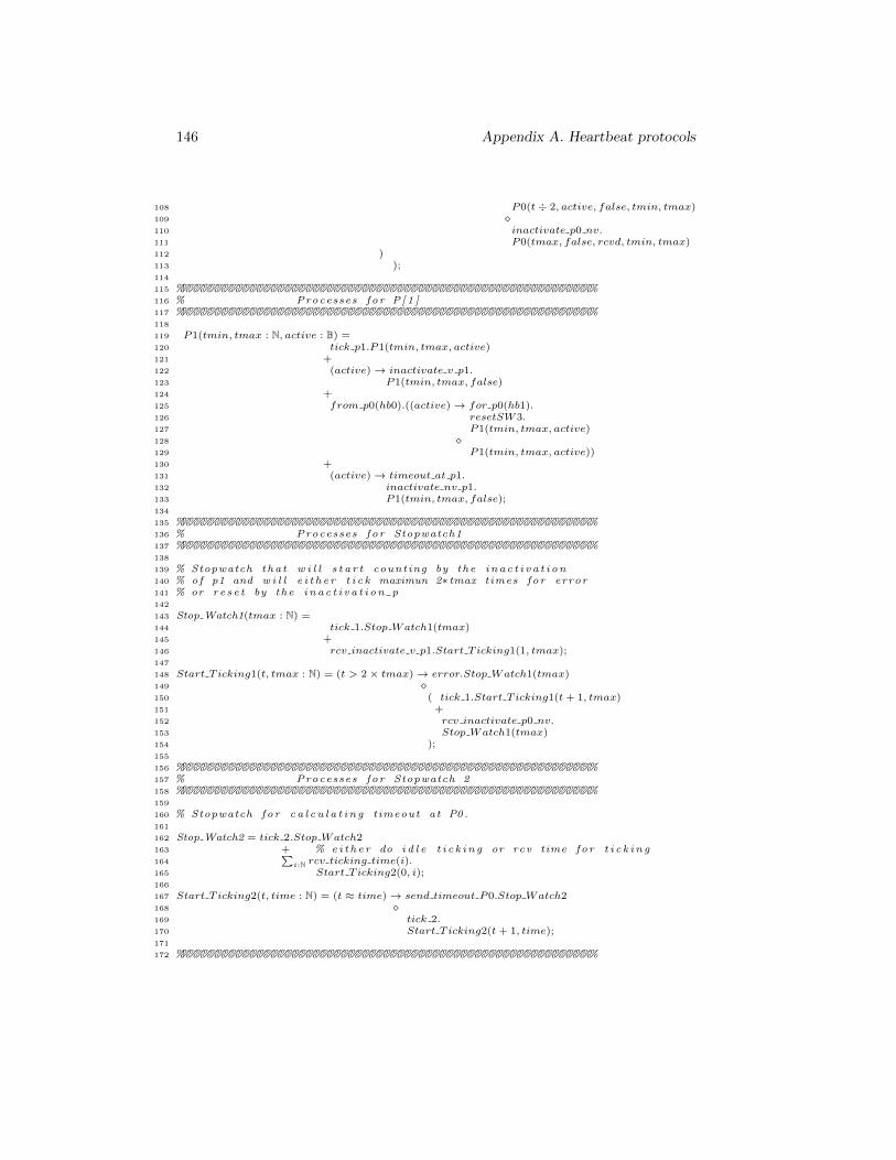
146 Appendix A. Heartbeat protocols
108 P0(t÷ 2, active, false, tmin, tmax)109 �110 inactivate p0 nv.111 P0(tmax, false, rcvd, tmin, tmax)112 )113 );114
115 %%%%%%%%%%%%%%%%%%%%%%%%%%%%%%%%%%%%%%%%%%%%%%%%%%%%%%%%%%%%116 % Processes for P[ 1 ]117 %%%%%%%%%%%%%%%%%%%%%%%%%%%%%%%%%%%%%%%%%%%%%%%%%%%%%%%%%%%%118
119 P1(tmin, tmax : N, active : B) =120 tick p1.P1(tmin, tmax, active)121 +122 (active)→ inactivate v p1.123 P1(tmin, tmax, false)124 +125 from p0(hb0).((active)→ for p0(hb1).126 resetSW3.127 P1(tmin, tmax, active)128 �129 P1(tmin, tmax, active))130 +131 (active)→ timeout at p1.132 inactivate nv p1.133 P1(tmin, tmax, false);134
135 %%%%%%%%%%%%%%%%%%%%%%%%%%%%%%%%%%%%%%%%%%%%%%%%%%%%%%%%%%%%136 % Processes for Stopwatch1137 %%%%%%%%%%%%%%%%%%%%%%%%%%%%%%%%%%%%%%%%%%%%%%%%%%%%%%%%%%%%138
139 % Stopwatch tha t w i l l s t a r t counting by the i n a c t i v a t i o n140 % of p1 and w i l l e i t h e r t i c k maximun 2∗tmax times for error141 % or r e s e t by the i n a c t i v a t i o n p142
143 Stop Watch1(tmax : N) =144 tick 1.Stop Watch1(tmax)145 +146 rcv inactivate v p1.Start T icking1(1, tmax);147
148 Start T icking1(t, tmax : N) = (t > 2× tmax)→ error.Stop Watch1(tmax)149 �150 ( tick 1.Start T icking1(t+ 1, tmax)151 +152 rcv inactivate p0 nv.153 Stop Watch1(tmax)154 );155
156 %%%%%%%%%%%%%%%%%%%%%%%%%%%%%%%%%%%%%%%%%%%%%%%%%%%%%%%%%%%%157 % Processes for Stopwatch 2158 %%%%%%%%%%%%%%%%%%%%%%%%%%%%%%%%%%%%%%%%%%%%%%%%%%%%%%%%%%%%159
160 % Stopwatch for c a l c u l a t i n g timeout at P0.161
162 Stop Watch2 = tick 2.Stop Watch2163 + % e i t h e r do i d l e t i c k i n g or rcv time for t i c k i n g164
∑i:N rcv ticking time(i).
165 Start T icking2(0, i);166
167 Start T icking2(t, time : N) = (t ≈ time)→ send timeout P0.Stop Watch2168 �169 tick 2.170 Start T icking2(t+ 1, time);171
172 %%%%%%%%%%%%%%%%%%%%%%%%%%%%%%%%%%%%%%%%%%%%%%%%%%%%%%%%%%%%
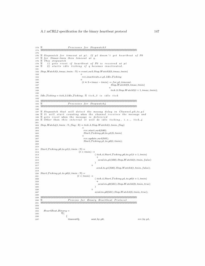
A.1 mCRL2 specification for the binary heartbeat protocol 147
173 % Processes for Stopwatch3174 %%%%%%%%%%%%%%%%%%%%%%%%%%%%%%%%%%%%%%%%%%%%%%%%%%%%%%%%%%%%175
176 % Stopwatch for timeout at p1 . I f p1 doesn ’ t ge t hear tbeat of P0177 % for 3tmax−tmin then timeout at q .178 % This stopwatch179 % 1) ge t s r e s e t i f hear tbeat of P0 i s rece ived at p1180 % 2) s t a r t s i d l e t i c k i n g i f q becomes i n a c t i v a t e d .181
182 Stop Watch3(t, tmax, tmin : N) = reset sw3.Stop Watch3(0, tmax, tmin)183 +184 rcv inactivate v p1.Idle T icking185 +186 (t ≈ 3 ∗ tmax− tmin)→ for p1 timeout.187 Stop Watch3(0, tmax, tmin)188 �189 tick 3.Stop Watch3(t+ 1, tmax, tmin);190
191 Idle T icking = tick 3.Idle T icking; % t i c k 3 i s i d l e t i c k192
193 %%%%%%%%%%%%%%%%%%%%%%%%%%%%%%%%%%%%%%%%%%%%%%%%%%%%%%%%%%%%194 % Processes for Stopwatch4195 %%%%%%%%%%%%%%%%%%%%%%%%%%%%%%%%%%%%%%%%%%%%%%%%%%%%%%%%%%%%196
197 % Stopwatch tha t w i l l de t ec t the messag delay in Channel p0 to p1198 % I t w i l l s t a r t counting when the channel r ec e i ve s the message and199 % get s r e s e t when the message i s d e l i v e r e d200 % Other than t h i s i n t e r v a l i t w i l l do i d l e t i ck ing , i . e . , t i c k 4201
202 Stop Watch4(t, tmin : N, flag : B) = tick 4.Stop Watch4(t, tmin, flag)203 +204 rcv start sw4(hb0).205 Start T icking p0 to p1(0, tmin)206 +207 rcv update sw4(hb1).208 Start T icking p1 to p0(t, tmin);209
210
211 Start T icking p0 to p1(t, tmin : N) =212 (t < tmin)→213 ( tick 4.Start T icking p0 to p1(t+ 1, tmin)214 +215 send to p1(hb0).Stop Watch4(t, tmin, false)216 )217 �218 send to p1(hb0).Stop Watch4(t, tmin, false);219
220 Start T icking p1 to p0(t, tmin : N) =221 (t < tmin)→222 ( tick 4.Start T icking p1 to p0(t+ 1, tmin)223 +224 send to p0(hb1).Stop Watch4(0, tmin, true)225 )226 �227 send to p0(hb1).Stop Watch4(0, tmin, true);228
229 %%%%%%%%%%%%%%%%%%%%%%%%%%%%%%%%%%%%%%%%%%%%%%%%%%%%%%%%%%%%230 % Process for Binary Heartbeat Protocol231 %%%%%%%%%%%%%%%%%%%%%%%%%%%%%%%%%%%%%%%%%%%%%%%%%%%%%%%%%%%%232
233
234 HeartBeat Binary =235 ∇(236 {237 timeoutQ, sent by p0, rcv by p1,
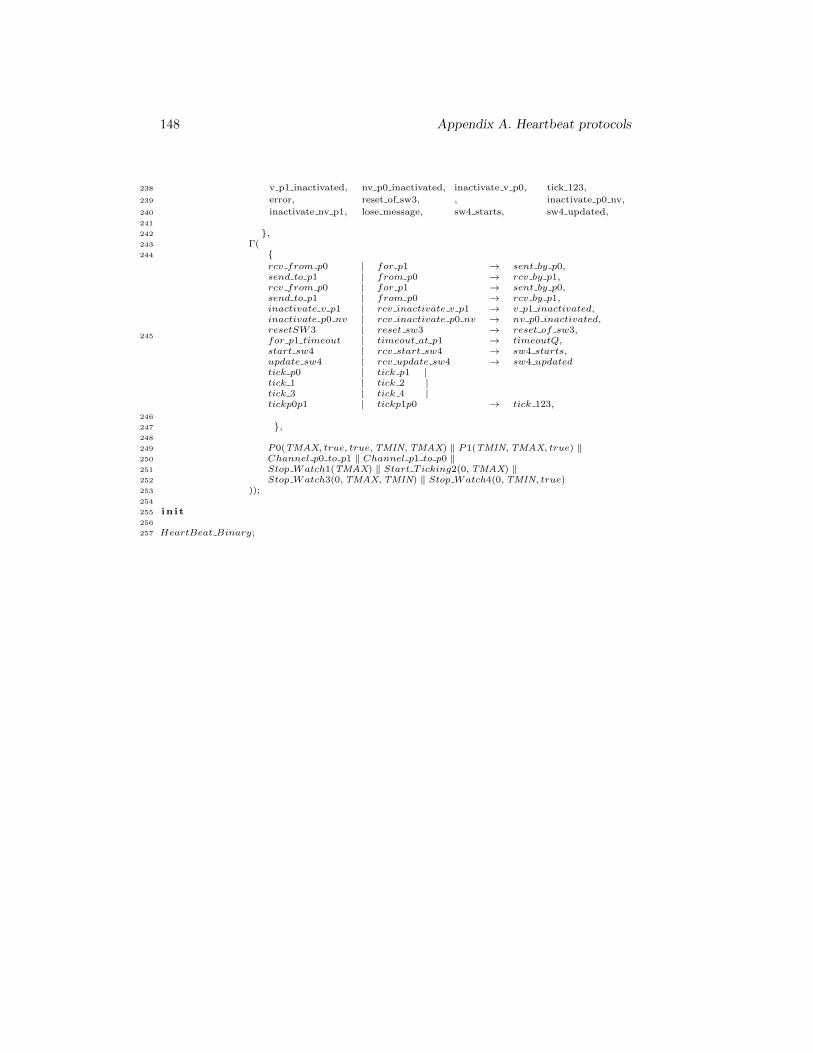
148 Appendix A. Heartbeat protocols
238 v p1 inactivated, nv p0 inactivated, inactivate v p0, tick 123,
239 error, reset of sw3, , inactivate p0 nv,
240 inactivate nv p1, lose message, sw4 starts, sw4 updated,241
242 },243 Γ(244 {
245
rcv from p0 | for p1 → sent by p0,send to p1 | from p0 → rcv by p1,rcv from p0 | for p1 → sent by p0,send to p1 | from p0 → rcv by p1,inactivate v p1 | rcv inactivate v p1 → v p1 inactivated,inactivate p0 nv | rcv inactivate p0 nv → nv p0 inactivated,resetSW3 | reset sw3 → reset of sw3,for p1 timeout | timeout at p1 → timeoutQ,start sw4 | rcv start sw4 → sw4 starts,update sw4 | rcv update sw4 → sw4 updatedtick p0 | tick p1 |tick 1 | tick 2 |tick 3 | tick 4 |tickp0p1 | tickp1p0 → tick 123,
246
247 },248
249 P0(TMAX, true, true,TMIN,TMAX) ‖ P1(TMIN,TMAX, true) ‖250 Channel p0 to p1 ‖ Channel p1 to p0 ‖251 Stop Watch1(TMAX) ‖ Start T icking2(0,TMAX) ‖252 Stop Watch3(0,TMAX,TMIN) ‖ Stop Watch4(0,TMIN, true)253 ));254
255 in i t256
257 HeartBeat Binary;
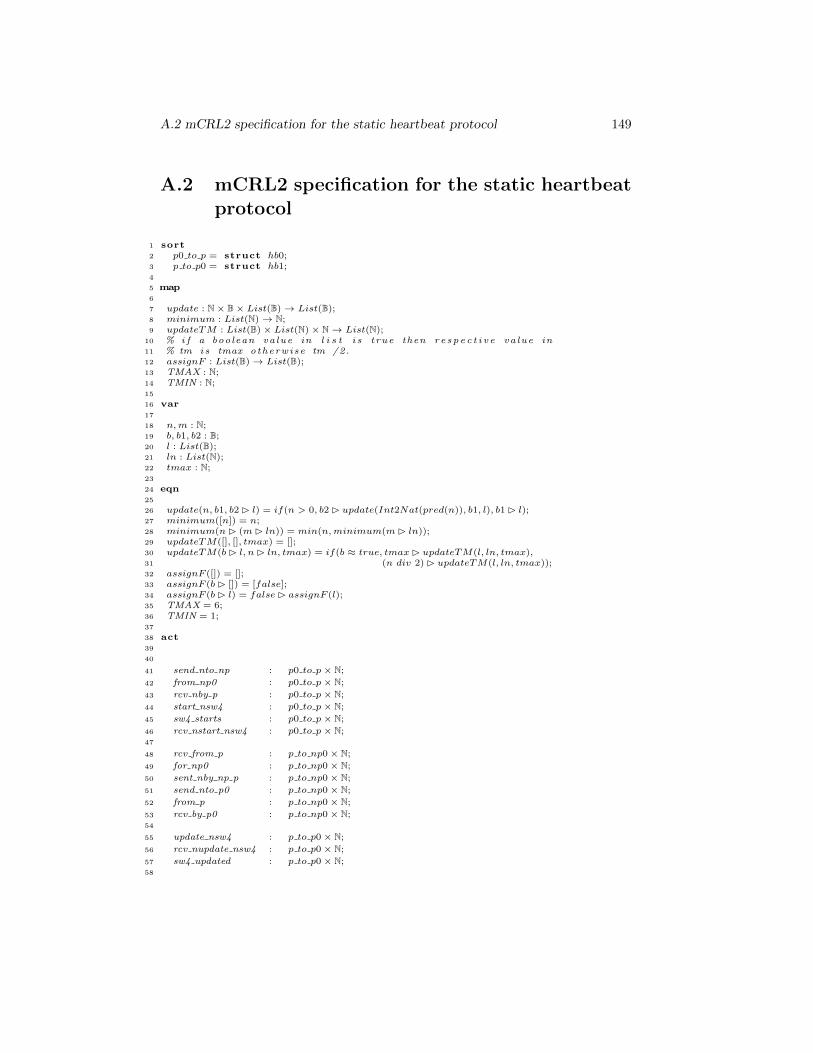
A.2 mCRL2 specification for the static heartbeat protocol 149
A.2 mCRL2 specification for the static heartbeatprotocol
1 sort2 p0 to p = struct hb0;3 p to p0 = struct hb1;4
5 map6
7 update : N× B× List(B)→ List(B);8 minimum : List(N)→ N;9 updateTM : List(B)× List(N)× N→ List(N);
10 % i f a boolean value in l i s t i s true then r e s p e c t i v e value in11 % tm i s tmax otherwise tm /2.12 assignF : List(B)→ List(B);13 TMAX : N;14 TMIN : N;15
16 var17
18 n,m : N;19 b, b1, b2 : B;20 l : List(B);21 ln : List(N);22 tmax : N;23
24 eqn25
26 update(n, b1, b2 � l) = if(n > 0, b2 � update(Int2Nat(pred(n)), b1, l), b1 � l);27 minimum([n]) = n;28 minimum(n� (m� ln)) = min(n,minimum(m� ln));29 updateTM([], [], tmax) = [];30 updateTM(b� l, n� ln, tmax) = if(b ≈ true, tmax� updateTM(l, ln, tmax),31 (n div 2) � updateTM(l, ln, tmax));32 assignF ([]) = [];33 assignF (b� []) = [false];34 assignF (b� l) = false� assignF (l);35 TMAX = 6;36 TMIN = 1;37
38 act39
40
41 send nto np : p0 to p× N;
42 from np0 : p0 to p× N;
43 rcv nby p : p0 to p× N;
44 start nsw4 : p0 to p× N;
45 sw4 starts : p0 to p× N;
46 rcv nstart nsw4 : p0 to p× N;47
48 rcv from p : p to np0× N;
49 for np0 : p to np0× N;
50 sent nby np p : p to np0× N;
51 send nto p0 : p to np0× N;
52 from p : p to np0× N;
53 rcv by p0 : p to np0× N;54
55 update nsw4 : p to p0× N;
56 rcv nupdate nsw4 : p to p0× N;
57 sw4 updated : p to p0× N;58
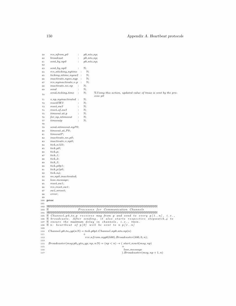
150 Appendix A. Heartbeat protocols
59 rcv nfrom p0 : p0 nto np;
60 broadcast : p0 nto np;
61 sent by np0 : p0 nto np;62
63 sent by np0 : N;
64 rcv nticking nytime : N;
65 ticking ntime nysw2 : N;
66 inactivate nynv nyp : N;
67 rcv nyinactivate v p : N;
68 inactivate nv np : N;
69 send : N;
70send ticking time : N; %Using this action, updated value of tmax is sent by the pro-
cess p0
71 v np nyinactivated : N;
72 resetSW3 : N;
73 reset sw3 : N;
74 reset of sw3 : N;
75 timeout at p : N;
76 for np ntimeout : N;
77 timeoutp : N;78
79 send ntimeout nyP0 ;
80 timeout at P0 ;
81 timeoutP ;
82 inactivate nv p0 ;
83 inactivate v np0 ;
84 tick n123 ;
85 tick p0 ;
86 tick p;
87 tick 1 ;
88 tick 2 ;
89 tick 3 ;
90 tick p0p1 ;
91 tick p1p0 ;
92 tick n4 ;
93 nv np0 inactivated;
94 lose message;
95 reset sw1 ;
96 rcv reset sw1 ;
97 sw1 nreset;
98 error ;99
100 proc101
102 %%%%%%%%%%%%%%%%%%%%%%%%%%%%%%%%%%%%%%%%%%%%%%%%%%%%%%%%%%%%103 % Processes for Communication Channels104 %%%%%%%%%%%%%%%%%%%%%%%%%%%%%%%%%%%%%%%%%%%%%%%%%%%%%%%%%%%%105 % Channel p0 to p r ec e i ve s msg from p and send to every p [ 1 . . n ] , i . e . ,106 % broadcasts . After sending , i t a l so s t a r t s r e s p e c t i v e stopwatch 4 to107 % ensure the maximum delay in channels , i . e . , tmin .108 % n : heartbeat of p [ 0 ] w i l l be sent to n p [ 1 . . n ]109
110 Channel p0 tonyp(n:N) = tick p0p1.Channel np0 nto np(n)111 +112 rcv nfrom nyp0(hb0).Broadcaster(hb0, 0, n);113
114 Broadcaster(msg:p0nytonyp, np, n:N) = (np < n)→ ( start nsw4(msg, np)115 +116 lose message117 ).Broadcaster(msg, np+ 1, n)
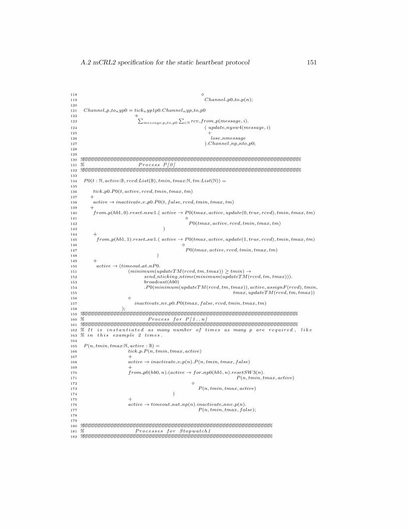
A.2 mCRL2 specification for the static heartbeat protocol 151
118 �119 Channel p0 to p(n);120
121 Channel p tonyp0 = ticknyp1p0.Channelnyp to p0122 +123
∑message:p to p0
∑i:N rcv from p(message, i).
124 ( update nysw4(message, i)125 +126 lose nmessage127 ).Channel np nto p0;128
129
130 %%%%%%%%%%%%%%%%%%%%%%%%%%%%%%%%%%%%%%%%%%%%%%%%%%%%%%%%%%%%%%%%%%%%%131 % Process P[ 0 ]132 %%%%%%%%%%%%%%%%%%%%%%%%%%%%%%%%%%%%%%%%%%%%%%%%%%%%%%%%%%%%%%%%%%%%%133
134 P0(t : N, active:B, rcvd:List(B), tmin, tmax:N, tm:List(N)) =135
136 tick p0.P0(t, active, rcvd, tmin, tmax, tm)137 +138 active→ inactivate v p0.P0(t, false, rcvd, tmin, tmax, tm)139 +140 from p(hb1, 0).reset nsw1.( active→ P0(tmax, active, update(0, true, rcvd), tmin, tmax, tm)141 �142 P0(tmax, active, rcvd, tmin, tmax, tm)143 )144 +145 from p(hb1, 1).reset sw1.( active→ P0(tmax, active, update(1, true, rcvd), tmin, tmax, tm)146 �147 P0(tmax, active, rcvd, tmin, tmax, tm)148 )149 +150 active→ (timeout at nP0.151 (minimum(updateTM(rcvd, tm, tmax)) ≥ tmin)→152 send nticking ntime(minimum(updateTM(rcvd, tm, tmax))).153 broadcast(hb0)154 .P0(minimum(updateTM(rcvd, tm, tmax)), active, assignF (rcvd), tmin,155 tmax, updateTM(rcvd, tm, tmax))156 �157 inactivate nv p0.P0(tmax, false, rcvd, tmin, tmax, tm)158 );159 %%%%%%%%%%%%%%%%%%%%%%%%%%%%%%%%%%%%%%%%%%%%%%%%%%%%%%%%%%%%%%%%%%%%160 % Process for P[ 1 . . n ]161 %%%%%%%%%%%%%%%%%%%%%%%%%%%%%%%%%%%%%%%%%%%%%%%%%%%%%%%%%%%%%%%%%%%%162 % I t i s i n s t a n t i a t e d as many number of times as many p are required , l i k e163 % in t h i s example 2 times .164
165 P (n, tmin, tmax:N, active : B) =166 tick p.P (n, tmin, tmax, active)167 +168 active→ inactivate v p(n).P (n, tmin, tmax, false)169 +170 from p0(hb0, n).(active→ for np0(hb1, n).resetSW3(n).171 P (n, tmin, tmax, active)172 �173 P (n, tmin, tmax, active)174 )175 +176 active→ timeout nat np(n).inactivate nnv p(n).177 P (n, tmin, tmax, false);178
179
180 %%%%%%%%%%%%%%%%%%%%%%%%%%%%%%%%%%%%%%%%%%%%%%%%%%%%%%%%%%%%181 % Processes for Stopwatch1182 %%%%%%%%%%%%%%%%%%%%%%%%%%%%%%%%%%%%%%%%%%%%%%%%%%%%%%%%%%%%
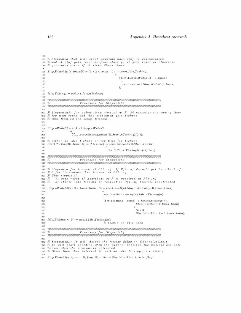
152 Appendix A. Heartbeat protocols
183
184 % Stopwatch tha t w i l l s t a r t counting when p [ 0 ] i s i n s t a n t i a t e d185 % and i f p [ 0 ] ge t s response from other p , i t ge t s r e s e t or otherwise186 % generates error i f i t t i c k s 2tmax times .187
188 Stop Watch1(t:N, tmax:N) = (t ≈ 2× tmax+ 1)→ error.Idle T icking1189 �190 ( tick 1.Stop Watch1(t+ 1, tmax)191 +192 rcv reset sw1.Stop Watch1(0, tmax)193 );194
195 Idle Ticking1 = tick n1 .Idle nTicking1 ;196
197 %%%%%%%%%%%%%%%%%%%%%%%%%%%%%%%%%%%%%%%%%%%%%%%%%%%%%%%%%%%%198 % Processes for Stopwatch2199 %%%%%%%%%%%%%%%%%%%%%%%%%%%%%%%%%%%%%%%%%%%%%%%%%%%%%%%%%%%%200
201 % Stopwatch2 : for c a l c u l a t i n g timeout at P. P0 computes the wating time202 % for next round and t h i s stopwatch ge t s t i c k i n g203 % time from P0 and sends timeout204
205
206 Stop nWatch2 = tick n2.Stop nWatch2207 +208
∑i:N .rcv nticking ntime(i).Start nTicking2(0, i);
209
210 % e i t h e r do i d l e t i c k i n g or rcv time for t i c k i n g211 Start T icking2(t, time : N) = (t ≈ time)→ send timeout P0.Stop Watch2212 �213 tick 2.Start T icking2(t+ 1, time);214
215 %%%%%%%%%%%%%%%%%%%%%%%%%%%%%%%%%%%%%%%%%%%%%%%%%%%%%%%%%%%%216 % Processes for Stopwatch3217 %%%%%%%%%%%%%%%%%%%%%%%%%%%%%%%%%%%%%%%%%%%%%%%%%%%%%%%%%%%%218
219 % Stopwatch for timeout at P[ 1 . . n ] . I f P [ 1 . . n ] doesn ’ t ge t hear tbeat of220 % P for 3tmax−tmin then timeout at P[ 1 . . n ] .221 % This stopwatch222 % 1) ge t s r e s e t i f hear tbeat of P i s rece ived at P[ 1 . . n ]223 % 2) s t a r t s i d l e t i c k i n g i f r e s p e c t i v e P[ 1 . . n ] becomes i n a c t i v a t e d .224
225 Stop nWatch3(n : N, t, tmax, tmin : N) = reset nsw3(n).Stop nWatch3(n, 0, tmax, tmin)226 +227 rcv inactivate nv np(n).Idle nTicking(n)228 +229 (t ≈ 3× tmax− tmin)→ for np timeout(n).230 Stop Watch3(n, 0, tmax, tmin)231 �232 tick 3.233 Stop Watch3(n, t+ 1, tmax, tmin);234
235 Idle T icking(n : N) = tick 3.Idle T icking(n);236 % t i c k 3 i s i d l e t i c k237
238 %%%%%%%%%%%%%%%%%%%%%%%%%%%%%%%%%%%%%%%%%%%%%%%%%%%%%%%%%%%%239 % Processes for Stopwatch4240 %%%%%%%%%%%%%%%%%%%%%%%%%%%%%%%%%%%%%%%%%%%%%%%%%%%%%%%%%%%%241
242 % Stopwatch4 : I t w i l l de t ec t the messag de lay in Channel p0 to p243 % I t w i l l s t a r t counting when the channel r ec e i v e s the message and ge t s244 %r e s e t when the message i s d e l i v e r e d245 % Other than t h i s i n t e r v a l i t w i l l do i d l e t i ck ing , i . e t i c k 4246
247 Stop Watch4(n, t, tmin : N, flag : B) = tick 4.Stop Watch4(n, t, tmin, flag)
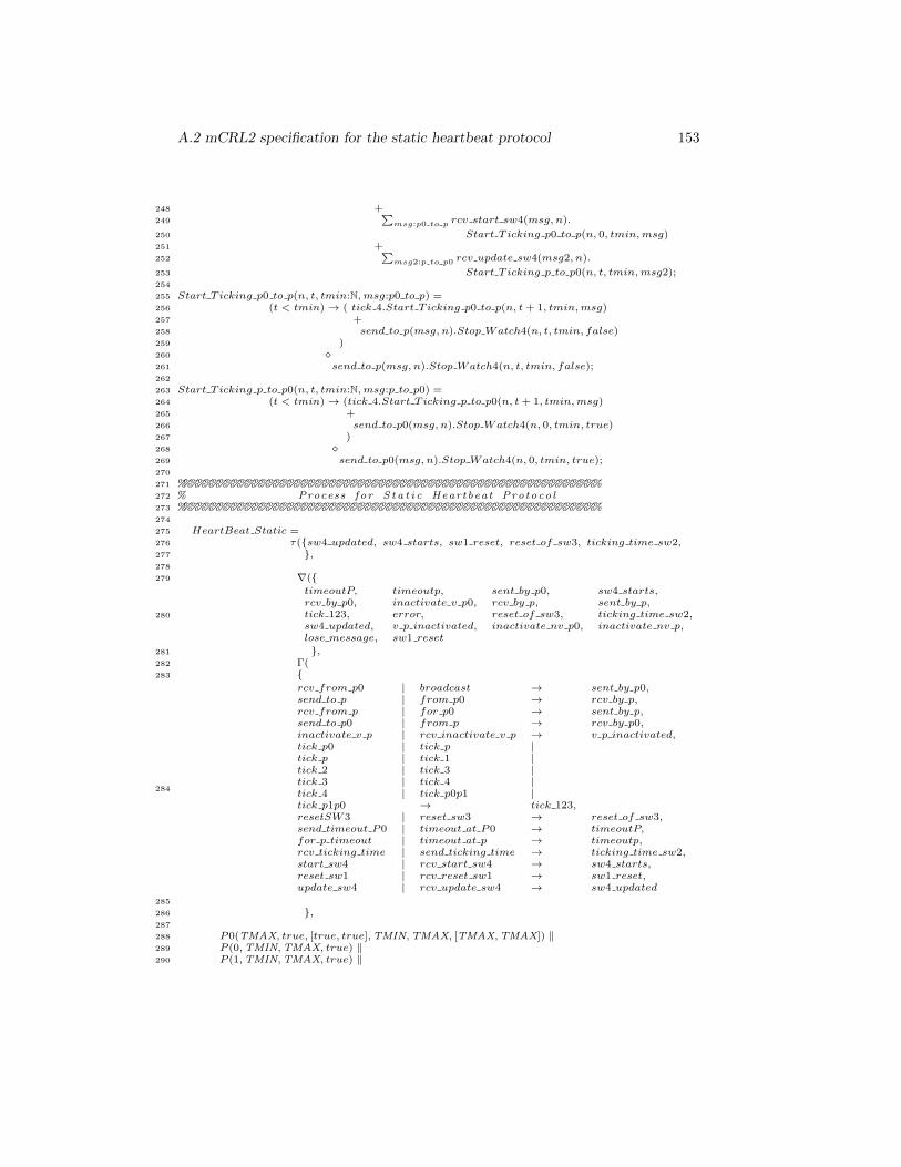
A.2 mCRL2 specification for the static heartbeat protocol 153
248 +249
∑msg:p0 to p rcv start sw4(msg, n).
250 Start T icking p0 to p(n, 0, tmin,msg)251 +252
∑msg2:p to p0 rcv update sw4(msg2, n).
253 Start T icking p to p0(n, t, tmin,msg2);254
255 Start T icking p0 to p(n, t, tmin:N,msg:p0 to p) =256 (t < tmin)→ ( tick 4.Start T icking p0 to p(n, t+ 1, tmin,msg)257 +258 send to p(msg, n).Stop Watch4(n, t, tmin, false)259 )260 �261 send to p(msg, n).Stop Watch4(n, t, tmin, false);262
263 Start T icking p to p0(n, t, tmin:N,msg:p to p0) =264 (t < tmin)→ (tick 4.Start T icking p to p0(n, t+ 1, tmin,msg)265 +266 send to p0(msg, n).Stop Watch4(n, 0, tmin, true)267 )268 �269 send to p0(msg, n).Stop Watch4(n, 0, tmin, true);270
271 %%%%%%%%%%%%%%%%%%%%%%%%%%%%%%%%%%%%%%%%%%%%%%%%%%%%%%%%%%%%272 % Process for S t a t i c Heartbeat Protocol273 %%%%%%%%%%%%%%%%%%%%%%%%%%%%%%%%%%%%%%%%%%%%%%%%%%%%%%%%%%%%274
275 HeartBeat Static =276 τ({sw4 updated, sw4 starts, sw1 reset, reset of sw3, ticking time sw2,277 },278
279 ∇({
280
timeoutP, timeoutp, sent by p0, sw4 starts,rcv by p0, inactivate v p0, rcv by p, sent by p,tick 123, error, reset of sw3, ticking time sw2,sw4 updated, v p inactivated, inactivate nv p0, inactivate nv p,lose message, sw1 reset
281 },282 Γ(283 {
284
rcv from p0 | broadcast → sent by p0,send to p | from p0 → rcv by p,rcv from p | for p0 → sent by p,send to p0 | from p → rcv by p0,inactivate v p | rcv inactivate v p → v p inactivated,tick p0 | tick p |tick p | tick 1 |tick 2 | tick 3 |tick 3 | tick 4 |tick 4 | tick p0p1 |tick p1p0 → tick 123,resetSW3 | reset sw3 → reset of sw3,send timeout P0 | timeout at P0 → timeoutP,for p timeout | timeout at p → timeoutp,rcv ticking time | send ticking time → ticking time sw2,start sw4 | rcv start sw4 → sw4 starts,reset sw1 | rcv reset sw1 → sw1 reset,update sw4 | rcv update sw4 → sw4 updated
285
286 },287
288 P0(TMAX, true, [true, true],TMIN,TMAX, [TMAX,TMAX]) ‖289 P (0,TMIN,TMAX, true) ‖290 P (1,TMIN,TMAX, true) ‖
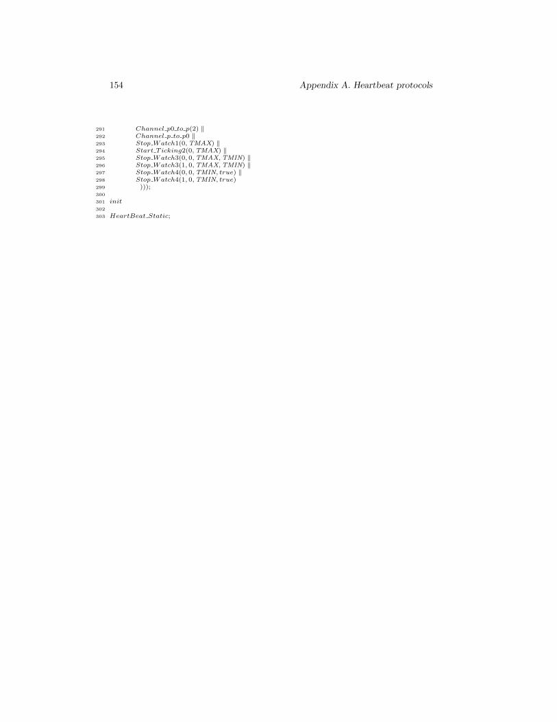
154 Appendix A. Heartbeat protocols
291 Channel p0 to p(2) ‖292 Channel p to p0 ‖293 Stop Watch1(0,TMAX) ‖294 Start T icking2(0,TMAX) ‖295 Stop Watch3(0, 0,TMAX,TMIN) ‖296 Stop Watch3(1, 0,TMAX,TMIN) ‖297 Stop Watch4(0, 0,TMIN, true) ‖298 Stop Watch4(1, 0,TMIN, true)299 )));300
301 init302
303 HeartBeat Static;
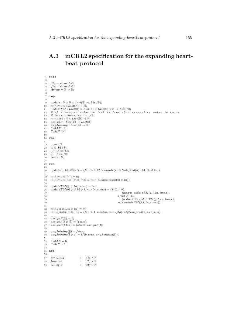
A.3 mCRL2 specification for the expanding heartbeat protocol 155
A.3 mCRL2 specification for the expanding heart-beat protocol
1 sort2
3 p2q = structhb0;4 q2p = structhb1;5 Array = N→ N;6
7 map8
9 update : N× B× List(B)→ List(B);10 minimum : List(N)→ N;11 updateTM : List(B)× List(B)× List(N)× N→ List(N);12 % i f a boolean value in l i s t i s true then r e s p e c t i v e value in tm i s13 % tmax otherwise tm /2.14 minupto : N× List(N)→ N;15 assignF : List(B)→ List(B);16 anyJoining : List(B)→ B;17 TMAX : N;18 TMIN : N;19
20 var21
22 n,m : N;23 b, b1, b2 : B;24 l, j : List(B);25 ln : List(N);26 tmax : N;27
28 eqn29
30 update(n, b1, b2 � l) = if(n > 0, b2 � update(Int2Nat(pred(n)), b1, l), b1 � l);31
32 minimum([n]) = n;33 minimum(n� (m� ln)) = min(n,minimum(m� ln));34
35 updateTM([], [], ln, tmax) = ln;36 updateTM(b1 � j, b2 � l, n� ln, tmax) = if(b1 ∧ b2,37 tmax� updateTM (j, l, ln, tmax),38 if(b1 ∧ ¬b2,39 (n div 2) � updateTM (j, l, ln, tmax),40 n� updateTM (j, l, ln, tmax)));41
42 minupto(1,m� ln) = m;43 minupto(n,m� ln) = if(n > 1,min(m,minupto(Int2Nat(pred(n)), ln)),m);44
45 assignF ([]) = [];46 assignF (b� []) = [false];47 assignF (b� l) = false � assignF (l);48
49 anyJoining([]) = false;50 anyJoining(b� l) = if(b, true, anyJoining(l));51
52 TMAX = 6;53 TMIN = 1;54
55 act56
57 send to q : p2q × N;
58 from p0 : p2q × N;
59 rcv by p : p2q × N;
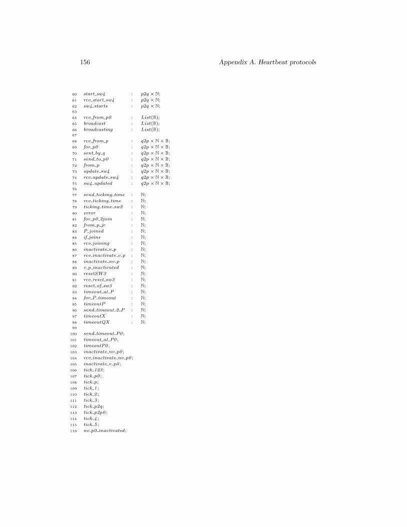
156 Appendix A. Heartbeat protocols
60 start sw4 : p2q × N;
61 rcv start sw4 : p2q × N;
62 sw4 starts : p2q × N;63
64 rcv from p0 : List(B);
65 broadcast : List(B);
66 broadcasting : List(B);67
68 rcv from p : q2p× N× B;
69 for p0 : q2p× N× B;
70 sent by q : q2p× N× B;
71 send to p0 : q2p× N× B;
72 from p : q2p× N× B;
73 update sw4 : q2p× N× B;
74 rcv update sw4 : q2p× N× B;
75 sw4 updated : q2p× N× B;76
77 send ticking time : N;
78 rcv ticking time : N;
79 ticking time sw2 : N;
80 error : N;
81 for p0 2join : N;
82 from p jr : N;
83 P joined : N;
84 if joins : N;
85 rcv joining : N;
86 inactivate v p : N;
87 rcv inactivate v p : N;
88 inactivate nv p : N;
89 v p inactivated : N;
90 resetSW3 : N;
91 rcv reset sw3 : N;
92 reset of sw3 : N;
93 timeout at P : N;
94 for P timeout : N;
95 timeoutP : N;
96 send timeout 2 P : N;
97 timeoutX : N;
98 timeoutQX : N;99
100 send timeout P0 ;
101 timeout at P0 ;
102 timeoutP0 ;
103 inactivate nv p0 ;
104 rcv inactivate nv p0 ;
105 inactivate v p0 ;
106 tick 123 ;
107 tick p0 ;
108 tick p;
109 tick 1 ;
110 tick 2 ;
111 tick 3 ;
112 tick p2q;
113 tick p2p0 ;
114 tick 4 ;
115 tick 5 ;
116 nv p0 inactivated;
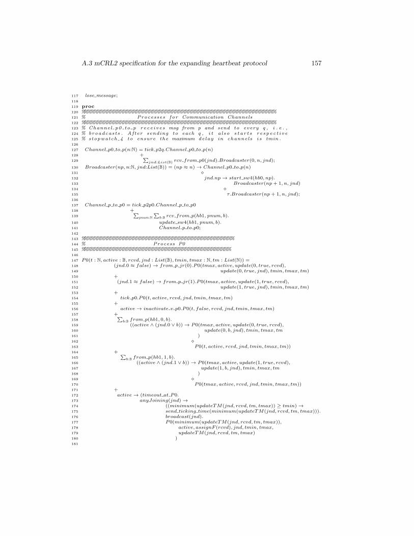
A.3 mCRL2 specification for the expanding heartbeat protocol 157
117 lose message;118
119 proc120 %%%%%%%%%%%%%%%%%%%%%%%%%%%%%%%%%%%%%%%%%%%%%%%%%%%%%%%%%%%%121 % Processes for Communication Channels122 %%%%%%%%%%%%%%%%%%%%%%%%%%%%%%%%%%%%%%%%%%%%%%%%%%%%%%%%%%%%123 % Channel p0 to p rec e i ve s msg from p and send to every q , i . e . ,124 % broadcasts . After sending to each q , i t a l so s t a r t s r e s p e c t i v e125 % stopwatch 4 to ensure the maximum delay in channels i s tmin .126
127 Channel p0 to p(n:N) = tick p2q.Channel p0 to p(n)128 +129
∑jnd:List(B) rcv from p0(jnd).Broadcaster(0, n, jnd);
130 Broadcaster(np, n:N, jnd:List(B)) = (np ≈ n)→ Channel p0 to p(n)131 �132 jnd.np→ start sw4(hb0, np).133 Broadcaster(np+ 1, n, jnd)134 �135 τ.Broadcaster(np+ 1, n, jnd);136
137 Channel p to p0 = tick p2p0.Channel p to p0138 +139
∑pnum:N
∑b:B rcv from p(hb1, pnum, b).
140 update sw4(hb1, pnum, b).141 Channel p to p0;142
143 %%%%%%%%%%%%%%%%%%%%%%%%%%%%%%%%%%%%%%%%%%%%%%%144 % Process P0145 %%%%%%%%%%%%%%%%%%%%%%%%%%%%%%%%%%%%%%%%%%%%%%146
147 P0(t : N, active : B, rcvd, jnd : List(B), tmin, tmax : N, tm : List(N)) =148 (jnd.0 ≈ false)→ from p jr(0).P0(tmax, active, update(0, true, rcvd),149 update(0, true, jnd), tmin, tmax, tm)150 +151 (jnd.1 ≈ false)→ from p jr(1).P0(tmax, active, update(1, true, rcvd),152 update(1, true, jnd), tmin, tmax, tm)153 +154 tick p0.P0(t, active, rcvd, jnd, tmin, tmax, tm)155 +156 active→ inactivate v p0.P0(t, false, rcvd, jnd, tmin, tmax, tm)157 +158
∑b:B from p(hb1, 0, b).
159 ((active ∧ (jnd.0 ∨ b))→ P0(tmax, active, update(0, true, rcvd),160 update(0, b, jnd), tmin, tmax, tm161 )162 �163 P0(t, active, rcvd, jnd, tmin, tmax, tm))164 +165
∑b:B from p(hb1, 1, b).
166 ((active ∧ (jnd.1 ∨ b))→ P0(tmax, active, update(1, true, rcvd),167 update(1, b, jnd), tmin, tmax, tm168 )169 �170 P0(tmax, active, rcvd, jnd, tmin, tmax, tm))171 +172 active→ (timeout at P0.173 anyJoining(jnd)→174 ((minimum(updateTM(jnd, rcvd, tm, tmax)) ≥ tmin)→175 send ticking time(minimum(updateTM(jnd, rcvd, tm, tmax))).176 broadcast(jnd).177 P0(minimum(updateTM(jnd, rcvd, tm, tmax)),178 active, assignF (rcvd), jnd, tmin, tmax,179 updateTM(jnd, rcvd, tm, tmax)180 )181
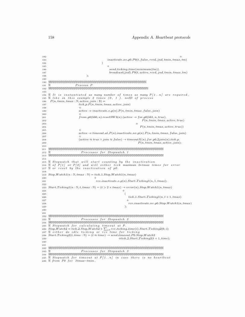
158 Appendix A. Heartbeat protocols
182 �183 inactivate nv p0.P0(t, false, rcvd, jnd, tmin, tmax, tm)184 )185 �186 send ticking time(minimum(tm)).187 broadcast(jnd).P0(t, active, rcvd, jnd, tmin, tmax, tm)188 );189
190 %%%%%%%%%%%%%%%%%%%%%%%%%%%%%%%%%%%%%%%%%%%%%%%%%%%191 % Process P192 %%%%%%%%%%%%%%%%%%%%%%%%%%%%%%%%%%%%%%%%%%%%%%%%%%%%193
194 % I t i s i n s t a n t i a t e d as many number of times as many P[ 1 . . n ] are required ,195 % l i k e in t h i s example 2 times (0 , 1 ) . n=ID of process196 P (n, tmin, tmax : N, active, join : B) =197 tick p.P (n, tmin, tmax, active, join)198 +199 active→ inactivate v p(n).P (n, tmin, tmax, false, join)200 +201 from p0(hb0, n).resetSW3(n).(active→ for p0(hb1, n, true).202 P (n, tmin, tmax, active, true)203 �204 P (n, tmin, tmax, active, true))205 +206 active→ timeout at P (n).inactivate nv p(n).P (n, tmin, tmax, false, join)207 +208 (active ≈ true ∧ join ≈ false)→ timeoutX(n).for p0 2join(n).tick p.209 P (n, tmin, tmax, active, join);210
211 %%%%%%%%%%%%%%%%%%%%%%%%%%%%%%%%%%%%%%%%%%%%%%%%%%%%%%%%%%%%212 % Processes for Stopwatch 1213 %%%%%%%%%%%%%%%%%%%%%%%%%%%%%%%%%%%%%%%%%%%%%%%%%%%%%%%%%%%%214
215 % Stopwatch tha t w i l l s t a r t counting by the i n a c t i v a t i o n216 % of P[ 1 ] or P[ 2 ] and w i l l e i t h e r t i c k maximun 2∗tmax times for error217 % or r e s e t by the i n a c t i v a t i o n of p0 .218
219 Stop Watch1(n : N, tmax : N) = tick 1.Stop Watch1(n, tmax)220 +221 rcv inactivate v p(n).Start T icking1(n, 1, tmax);222
223 Start T icking1(n : N, t, tmax : N) = (t > 2× tmax)→ error(n).Stop Watch1(n, tmax)224 �225 (226 tick 1.Start T icking1(n, t+ 1, tmax)227 +228 rcv inactivate nv p0.Stop Watch1(n, tmax)229 );230
231
232 %%%%%%%%%%%%%%%%%%%%%%%%%%%%%%%%%%%%%%%%%%%%%%%%%%%%%%%%%%%%233 % Processes for Stopwatch 2234 %%%%%%%%%%%%%%%%%%%%%%%%%%%%%%%%%%%%%%%%%%%%%%%%%%%%%%%%%%%%235 % Stopwatch for c a l c u l a t i n g timeout at P.236 Stop Watch2 = tick 2.Stop Watch2 +
∑i:N rcv ticking time(i).Start T icking2(0, i);
237 % e i t h e r do i d l e t i c k i n g or rcv time for t i c k i n g238 Start T icking2(t, time : N) = (t ≈ time)→ send timeout P0.Stop Watch2239 �tick 2.Start T icking2(t+ 1, time);240
241
242 %%%%%%%%%%%%%%%%%%%%%%%%%%%%%%%%%%%%%%%%%%%%%%%%%%%%%%%%%%%%243 % Processes for Stopwatch 3244 %%%%%%%%%%%%%%%%%%%%%%%%%%%%%%%%%%%%%%%%%%%%%%%%%%%%%%%%%%%%245 % Stopwatch for timeout at P[ 1 . . n ] in case there i s no heartbeat246 % from P0 for 3tmax−tmin .
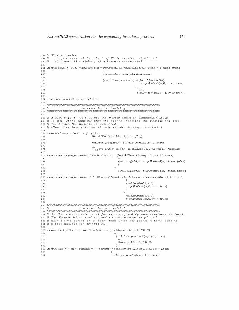
A.3 mCRL2 specification for the expanding heartbeat protocol 159
247 % This stopwatch248 % 1) ge t s r e s e t i f hear tbeat of P0 i s rece ived at P[ 1 . . n ]249 % 2) s t a r t s i d l e t i c k i n g i f q becomes i n a c t i v a t e d .250
251 Stop Watch3(n : N, t, tmax, tmin : N) = rcv reset sw3(n).tick 3.Stop Watch3(n, 0, tmax, tmin)252 +253 rcv inactivate v p(n).Idle T icking254 +255 (t ≈ 3× tmax− tmin)→ for P timeout(n).256 Stop Watch3(n, 0, tmax, tmin)257 �258 tick 3.259 Stop Watch3(n, t+ 1, tmax, tmin);260
261 Idle T icking = tick 3.Idle T icking;262
263 %%%%%%%%%%%%%%%%%%%%%%%%%%%%%%%%%%%%%%%%%%%%%%%%%%%%%%%%%%%%264 % Processes for Stopwatch 4265 %%%%%%%%%%%%%%%%%%%%%%%%%%%%%%%%%%%%%%%%%%%%%%%%%%%%%%%%%%%%266
267 % Stopwatch4 : I t w i l l de t ec t the messag de lay in Channel p0\ t o p268 % I t w i l l s t a r t counting when the channel r ec e i ve s the message and ge t s269 % r e s e t when the message i s d e l i v e r e d270 % Other than t h i s i n t e r v a l i t w i l l do i d l e t i ck ing , i . e t i c k 4271
272 Stop Watch4(n, t, tmin : N, flag : B) =273 tick 4.Stop Watch4(n, t, tmin, flag)274 +275 rcv start sw4(hb0, n).Start T icking p2q(n, 0, tmin)276 +277
∑b:B rcv update sw4(hb1, n, b).Start T icking q2p(n, t, tmin, b);
278
279 Start T icking p2q(n, t, tmin : N) = (t < tmin)→ (tick 4.Start T icking p2q(n, t+ 1, tmin)280 +281 send to q(hb0, n).Stop Watch4(n, t, tmin, false)282 )283 �284 send to q(hb0, n).Stop Watch4(n, t, tmin, false);285
286 Start T icking q2p(n, t, tmin : N, b : B) = (t < tmin)→ (tick 4.Start T icking q2p(n, t+ 1, tmin, b)287 +288 send to p0(hb1, n, b).289 Stop Watch4(n, 0, tmin, true)290 )291 �292 send to p0(hb1, n, b).293 Stop Watch4(n, 0, tmin, true);294
295 %%%%%%%%%%%%%%%%%%%%%%%%%%%%%%%%%%%%%%%%%%%%%%%%%%%%%%%%%%%%296 % Processes for Stopwatch 5297 %%%%%%%%%%%%%%%%%%%%%%%%%%%%%%%%%%%%%%%%%%%%%%%%%%%%%%%%%%%%298 % Another timeout introduced for expanding and dynamic hear tbeat pro toco l .299 % The Stopwatch5 i s used to send timeout message to p [ 1 . . n ]300 % when a time period of at l e a s t tmin uni t s has passed without sending301 % a beat message for jo in ing P0.302
303 StopwatchX(n:N, t:Int, tmax:N) = (t ≈ tmax)→ Stopwatch5(n, 0,TMIN)304 �305 (tick 5.StopwatchX(n, t+ 1, tmax)306 +307 Stopwatch5(n, 0,TMIN)308 );309 Stopwatch5(n:N, t:Int, tmin:N) = (t ≈ tmin)→ send timeout 2 P (n).Idle T ickingX(n)310 �311 tick 5.Stopwatch5(n, t+ 1, tmin);
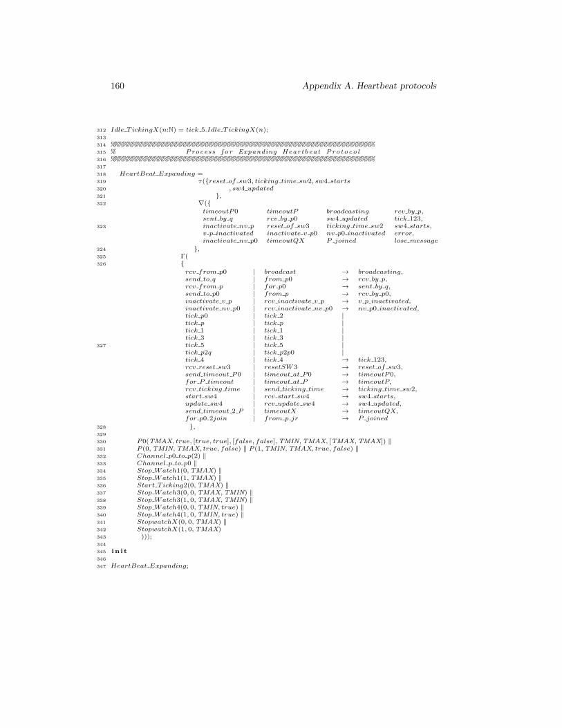
160 Appendix A. Heartbeat protocols
312 Idle T ickingX(n:N) = tick 5.Idle T ickingX(n);313
314 %%%%%%%%%%%%%%%%%%%%%%%%%%%%%%%%%%%%%%%%%%%%%%%%%%%%%%%%%%%%315 % Process for Expanding Heartbeat Protocol316 %%%%%%%%%%%%%%%%%%%%%%%%%%%%%%%%%%%%%%%%%%%%%%%%%%%%%%%%%%%%317
318 HeartBeat Expanding =319 τ({reset of sw3, ticking time sw2, sw4 starts320 , sw4 updated321 },322 ∇({
323
timeoutP0 timeoutP broadcasting rcv by p,sent by q rcv by p0 sw4 updated tick 123,inactivate nv p reset of sw3 ticking time sw2 sw4 starts,v p inactivated inactivate v p0 nv p0 inactivated error,inactivate nv p0 timeoutQX P joined lose message
324 },325 Γ(326 {
327
rcv from p0 | broadcast → broadcasting,send to q | from p0 → rcv by p,rcv from p | for p0 → sent by q,send to p0 | from p → rcv by p0,inactivate v p | rcv inactivate v p → v p inactivated,inactivate nv p0 | rcv inactivate nv p0 → nv p0 inactivated,tick p0 | tick 2 |tick p | tick p |tick 1 | tick 1 |tick 3 | tick 3 |tick 5 | tick 5 |tick p2q | tick p2p0 |tick 4 | tick 4 → tick 123,rcv reset sw3 | resetSW3 → reset of sw3,send timeout P0 | timeout at P0 → timeoutP0,for P timeout | timeout at P → timeoutP,rcv ticking time | send ticking time → ticking time sw2,start sw4 | rcv start sw4 → sw4 starts,update sw4 | rcv update sw4 → sw4 updated,send timeout 2 P | timeoutX → timeoutQX,for p0 2join | from p jr → P joined
328 },329
330 P0(TMAX, true, [true, true], [false, false],TMIN,TMAX, [TMAX,TMAX]) ‖331 P (0,TMIN,TMAX, true, false) ‖ P (1,TMIN,TMAX, true, false) ‖332 Channel p0 to p(2) ‖333 Channel p to p0 ‖334 Stop Watch1(0,TMAX) ‖335 Stop Watch1(1,TMAX) ‖336 Start T icking2(0,TMAX) ‖337 Stop Watch3(0, 0,TMAX,TMIN) ‖338 Stop Watch3(1, 0,TMAX,TMIN) ‖339 Stop Watch4(0, 0,TMIN, true) ‖340 Stop Watch4(1, 0,TMIN, true) ‖341 StopwatchX(0, 0,TMAX) ‖342 StopwatchX(1, 0,TMAX)343 )));344
345 in i t346
347 HeartBeat Expanding;
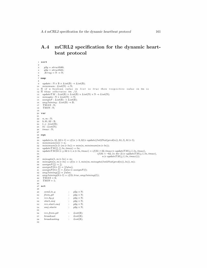
A.4 mCRL2 specification for the dynamic heartbeat protocol 161
A.4 mCRL2 specification for the dynamic heart-beat protocol
1 sort2
3 p2q = structhb0;4 q2p = structhb1;5 Array = N→ N;6
7 map8
9 update : N× B× List(B)→ List(B);10 minimum : List(N)→ N;11 % i f a boolean value in l i s t i s true then r e s p e c t i v e value in tm i s12 % tmax otherwise tm /2.13 updateTM : List(B)× List(B)× List(N)× N→ List(N);14 minupto : N× List(N)→ N;15 assignF : List(B)→ List(B);16 anyJoining : List(B)→ B;17 TMAX : N;18 TMIN : N;19
20 var21
22 n,m : N;23 b, b1, b2 : B;24 l, j : List(B);25 ln : List(N);26 tmax : N;27
28 eqn29
30 update(n, b1, b2 � l) = if(n > 0, b2 � update(Int2Nat(pred(n)), b1, l), b1 � l);31 minimum([n]) = n;32 minimum(n� (m� ln)) = min(n,minimum(m� ln));33 updateTM([], [], ln, tmax) = ln;34 updateTM(b1 � j, b2 � l, n� ln, tmax) = if(b1 ∧ b2, tmax� updateTM(j, l, ln, tmax),35 if(b1 ∧ ¬b2, (n div 2) � updateTM(j, l, ln, tmax),36 n� updateTM(j, l, ln, tmax)));37 minupto(1,m� ln) = m;38 minupto(n,m� ln) = if(n > 1,min(m,minupto(Int2Nat(pred(n)), ln)),m);39 assignF ([]) = [];40 assignF (b� []) = [false];41 assignF (b� l) = false� assignF (l);42 anyJoining([]) = false;43 anyJoining(b� l) = if(b, true, anyJoining(l));44 TMAX = 6;45 TMIN = 1;46
47 act48
49 send to q : p2q × N;
50 from p0 : p2q × N;
51 rcv by p : p2q × N;
52 start sw4 : p2q × N;
53 rcv start sw4 : p2q × N;
54 sw4 starts : p2q × N;55
56 rcv from p0 : List(B);
57 broadcast : List(B);
58 broadcasting : List(B);59
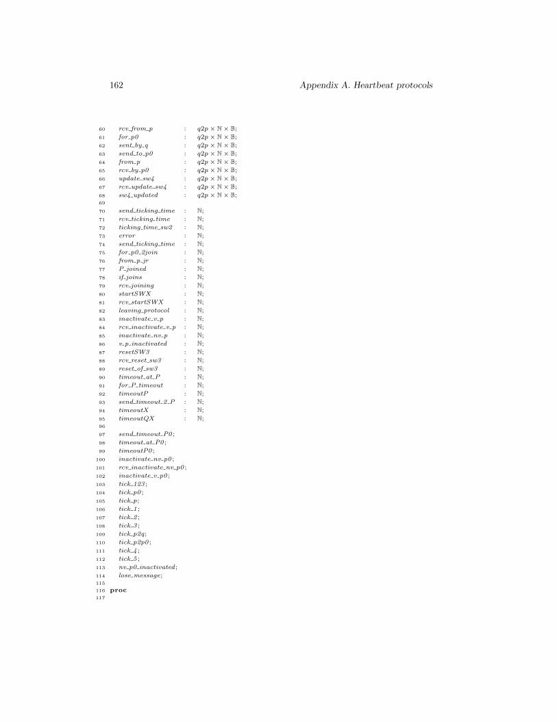
162 Appendix A. Heartbeat protocols
60 rcv from p : q2p× N× B;
61 for p0 : q2p× N× B;
62 sent by q : q2p× N× B;
63 send to p0 : q2p× N× B;
64 from p : q2p× N× B;
65 rcv by p0 : q2p× N× B;
66 update sw4 : q2p× N× B;
67 rcv update sw4 : q2p× N× B;
68 sw4 updated : q2p× N× B;69
70 send ticking time : N;
71 rcv ticking time : N;
72 ticking time sw2 : N;
73 error : N;
74 send ticking time : N;
75 for p0 2join : N;
76 from p jr : N;
77 P joined : N;
78 if joins : N;
79 rcv joining : N;
80 startSWX : N;
81 rcv startSWX : N;
82 leaving protocol : N;
83 inactivate v p : N;
84 rcv inactivate v p : N;
85 inactivate nv p : N;
86 v p inactivated : N;
87 resetSW3 : N;
88 rcv reset sw3 : N;
89 reset of sw3 : N;
90 timeout at P : N;
91 for P timeout : N;
92 timeoutP : N;
93 send timeout 2 P : N;
94 timeoutX : N;
95 timeoutQX : N;96
97 send timeout P0 ;
98 timeout at P0 ;
99 timeoutP0 ;
100 inactivate nv p0 ;
101 rcv inactivate nv p0 ;
102 inactivate v p0 ;
103 tick 123 ;
104 tick p0 ;
105 tick p;
106 tick 1 ;
107 tick 2 ;
108 tick 3 ;
109 tick p2q;
110 tick p2p0 ;
111 tick 4 ;
112 tick 5 ;
113 nv p0 inactivated;
114 lose message;115
116 proc117
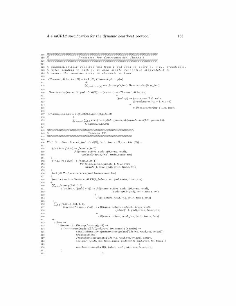
A.4 mCRL2 specification for the dynamic heartbeat protocol 163
118 %%%%%%%%%%%%%%%%%%%%%%%%%%%%%%%%%%%%%%%%%%%%%%%%%%%%%%%%%%%%119 % Processes for Communication Channels120 %%%%%%%%%%%%%%%%%%%%%%%%%%%%%%%%%%%%%%%%%%%%%%%%%%%%%%%%%%%%121
122 % Channel p0 to p rec e i ve s msg from p and send to every q , i . e . , broadcasts .123 % After sending to each q , i t a l so s t a r t s r e s p e c t i v e stopwatch 4 to124 % ensure the maximum delay in channels i s tmin .125
126 Channel p0 to p(n : N) = tick p2q.Channel p0 to p(n)127 +128
∑jnd:List(B) rcv from p0(jnd).Broadcaster(0, n, jnd);
129
130 Broadcaster(np, n : N, jnd : List(B)) = (np ≈ n)→ Channel p0 to p(n)131 �132 (jnd.np)→ (start sw4(hb0, np)).133 Broadcaster(np+ 1, n, jnd)134 �135 τ.Broadcaster(np+ 1, n, jnd);136
137 Channel p to p0 = tick p2p0.Channel p to p0138 +139
∑pnum:N
∑b:B rcv from p(hb1, pnum, b).(update sw4(hb1, pnum, b)).
140 Channel p to p0;141
142 %%%%%%%%%%%%%%%%%%%%%%%%%%%%%%%%%%%%%%%%%%%%%%%143 % Process P0144 %%%%%%%%%%%%%%%%%%%%%%%%%%%%%%%%%%%%%%%%%%%%%%145
146 P0(t : N, active : B, rcvd, jnd : List(B), tmin, tmax : N, tm : List(N)) =147
148 (jnd.0 ≈ false)→ from p jr(0).149 P0(tmax, active, update(0, true, rcvd),150 update(0, true, jnd), tmin, tmax, tm)151 +152 (jnd.1 ≈ false)→ from p jr(1).153 P0(tmax, active, update(1, true, rcvd),154 update(1, true, jnd), tmin, tmax, tm)155 +156 tick p0.P0(t, active, rcvd, jnd, tmin, tmax, tm)157 +158 (active)→ inactivate v p0.P0(t, false, rcvd, jnd, tmin, tmax, tm)159 +160
∑b:B from p(hb1, 0, b).
161 ((active ∧ (jnd.0 ∨ b))→ P0(tmax, active, update(0, true, rcvd),162 update(0, b, jnd), tmin, tmax, tm)163 �164 P0(t, active, rcvd, jnd, tmin, tmax, tm))165 +166
∑b:B from p(hb1, 1, b).
167 ((active ∧ (jnd.1 ∨ b))→ P0(tmax, active, update(1, true, rcvd),168 update(1, b, jnd), tmin, tmax, tm)169 �170 P0(tmax, active, rcvd, jnd, tmin, tmax, tm))171 +172 active→173 ( timeout at P0.anyJoining(jnd)→174 ( (minimum(updateTM(jnd, rcvd, tm, tmax)) ≥ tmin)→175 send ticking time(minimum(updateTM(jnd, rcvd, tm, tmax))).176 broadcast(jnd).177 P0(minimum(updateTM(jnd, rcvd, tm, tmax)), active,178 assignF (rcvd), jnd, tmin, tmax, updateTM(jnd, rcvd, tm, tmax))179 �180 inactivate nv p0.P0(t, false, rcvd, jnd, tmin, tmax, tm)181 )182 �
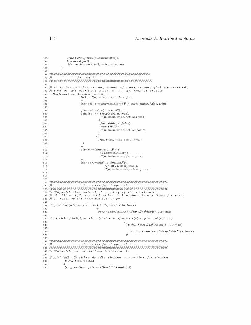
164 Appendix A. Heartbeat protocols
183 send ticking time(minimum(tm)).184 broadcast(jnd).185 P0(t, active, rcvd, jnd, tmin, tmax, tm)186 );187
188 %%%%%%%%%%%%%%%%%%%%%%%%%%%%%%%%%%%%%%%%%%%%%%%%%%%189 % Process P190 %%%%%%%%%%%%%%%%%%%%%%%%%%%%%%%%%%%%%%%%%%%%%%%%%%%%191
192 % I t i s i n s t a n t i a t e d as many number of times as many q ( s ) are required ,193 % l i k e in t h i s example 3 times (0 , 1 , 2) . n=ID of process194 P (n, tmin, tmax : N, active, join : B) =195 tick p.P (n, tmin, tmax, active, join)196 +197 (active)→ inactivate v p(n).P (n, tmin, tmax, false, join)198 +199 from p0(hb0, n).resetSW3(n).200 ( active→ ( for p0(hb1, n, true).201 P (n, tmin, tmax, active, true)202 +203 for p0(hb1, n, false).204 startSWX(n).205 P (n, tmin, tmax, active, false)206 )207 �208 P (n, tmin, tmax, active, true)209 )210 +211 active→ timeout at P (n).212 inactivate nv p(n).213 P (n, tmin, tmax, false, join)214 +215 (active ∧ ¬join)→ timeoutX(n).216 for p0 2join(n).tick p.217 P (n, tmin, tmax, active, join);218
219
220
221 %%%%%%%%%%%%%%%%%%%%%%%%%%%%%%%%%%%%%%%%%%%%%%%%%%%%%%%%%%%%222 % Processes for Stopwatch 1223 %%%%%%%%%%%%%%%%%%%%%%%%%%%%%%%%%%%%%%%%%%%%%%%%%%%%%%%%%%%%224 % Stopwatch tha t w i l l s t a r t counting by the i n a c t i v a t i o n225 % of P[ 1 ] or P[ 2 ] and w i l l e i t h e r t i c k maximun 2∗tmax times for error226 % or r e s e t by the i n a c t i v a t i o n of p0 .227
228 Stop Watch1(n:N, tmax:N) = tick 1.Stop Watch1(n, tmax)229 +230 rcv inactivate v p(n).Start T icking1(n, 1, tmax);231
232 Start T icking1(n:N, t, tmax:N) = (t > 2× tmax)→ error(n).Stop Watch1(n, tmax)233 �234 ( tick 1.Start T icking1(n, t+ 1, tmax)235 +236 rcv inactivate nv p0.Stop Watch1(n, tmax)237 );238
239 %%%%%%%%%%%%%%%%%%%%%%%%%%%%%%%%%%%%%%%%%%%%%%%%%%%%%%%%%%%%240 % Processes for Stopwatch 2241 %%%%%%%%%%%%%%%%%%%%%%%%%%%%%%%%%%%%%%%%%%%%%%%%%%%%%%%%%%%%242 % Stopwatch for c a l c u l a t i n g timeout at P.243
244 Stop Watch2 = % e i t h e r do i d l e t i c k i n g or rcv time for t i c k i n g245 tick 2.Stop Watch2246 +247
∑i:N rcv ticking time(i).Start T icking2(0, i);
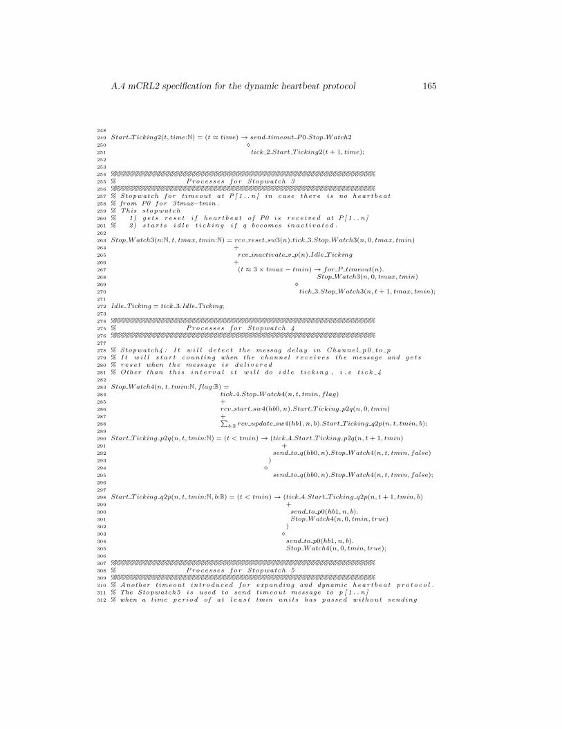
A.4 mCRL2 specification for the dynamic heartbeat protocol 165
248
249 Start T icking2(t, time:N) = (t ≈ time)→ send timeout P0.Stop Watch2250 �251 tick 2.Start T icking2(t+ 1, time);252
253
254 %%%%%%%%%%%%%%%%%%%%%%%%%%%%%%%%%%%%%%%%%%%%%%%%%%%%%%%%%%%%255 % Processes for Stopwatch 3256 %%%%%%%%%%%%%%%%%%%%%%%%%%%%%%%%%%%%%%%%%%%%%%%%%%%%%%%%%%%%257 % Stopwatch for timeout at P[ 1 . . n ] in case there i s no heartbeat258 % from P0 for 3tmax−tmin .259 % This stopwatch260 % 1) ge t s r e s e t i f hear tbeat of P0 i s rece ived at P[ 1 . . n ]261 % 2) s t a r t s i d l e t i c k i n g i f q becomes i n a c t i v a t e d .262
263 Stop Watch3(n:N, t, tmax, tmin:N) = rcv reset sw3(n).tick 3.Stop Watch3(n, 0, tmax, tmin)264 +265 rcv inactivate v p(n).Idle T icking266 +267 (t ≈ 3× tmax− tmin)→ for P timeout(n).268 Stop Watch3(n, 0, tmax, tmin)269 �270 tick 3.Stop Watch3(n, t+ 1, tmax, tmin);271
272 Idle Ticking = tick 3.Idle Ticking;273
274 %%%%%%%%%%%%%%%%%%%%%%%%%%%%%%%%%%%%%%%%%%%%%%%%%%%%%%%%%%%%275 % Processes for Stopwatch 4276 %%%%%%%%%%%%%%%%%%%%%%%%%%%%%%%%%%%%%%%%%%%%%%%%%%%%%%%%%%%%277
278 % Stopwatch4 : I t w i l l de t ec t the messag de lay in Channel p0 to p279 % I t w i l l s t a r t counting when the channel r ec e i ve s the message and ge t s280 % r e s e t when the message i s d e l i v e r e d281 % Other than t h i s i n t e r v a l i t w i l l do i d l e t i ck ing , i . e t i c k 4282
283 Stop Watch4(n, t, tmin:N, flag:B) =284 tick 4.Stop Watch4(n, t, tmin, flag)285 +286 rcv start sw4(hb0, n).Start T icking p2q(n, 0, tmin)287 +288
∑b:B rcv update sw4(hb1, n, b).Start T icking q2p(n, t, tmin, b);
289
290 Start T icking p2q(n, t, tmin:N) = (t < tmin)→ (tick 4.Start T icking p2q(n, t+ 1, tmin)291 +292 send to q(hb0, n).Stop Watch4(n, t, tmin, false)293 )294 �295 send to q(hb0, n).Stop Watch4(n, t, tmin, false);296
297
298 Start T icking q2p(n, t, tmin:N, b:B) = (t < tmin)→ (tick 4.Start T icking q2p(n, t+ 1, tmin, b)299 +300 send to p0(hb1, n, b).301 Stop Watch4(n, 0, tmin, true)302 )303 �304 send to p0(hb1, n, b).305 Stop Watch4(n, 0, tmin, true);306
307 %%%%%%%%%%%%%%%%%%%%%%%%%%%%%%%%%%%%%%%%%%%%%%%%%%%%%%%%%%%%308 % Processes for Stopwatch 5309 %%%%%%%%%%%%%%%%%%%%%%%%%%%%%%%%%%%%%%%%%%%%%%%%%%%%%%%%%%%%310 % Another timeout introduced for expanding and dynamic hear tbeat pro toco l .311 % The Stopwatch5 i s used to send timeout message to p [ 1 . . n ]312 % when a time period of at l e a s t tmin uni t s has passed without sending
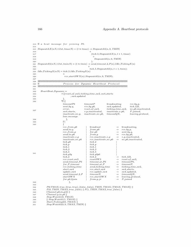
166 Appendix A. Heartbeat protocols
313 % a beat message for jo in ing P0.314
315 StopwatchX(n:N, t:Int, tmax:N) = (t ≈ tmax)→ Stopwatch5(n, 0,TMIN)316 �317 (tick 5.StopwatchX(n, t+ 1, tmax)318 +319 Stopwatch5(n, 0,TMIN)320 );321 Stopwatch5(n:N, t:Int, tmin:N) = (t ≈ tmin)→ send timeout 2 P (n).Idle T ickingX(n)322 �323 tick 5.Stopwatch5(n, t+ 1, tmin);324 Idle T ickingX(n:N) = tick 5.Idle T ickingX(n)325 +326 rcv startSWX(n).Stopwatch5(n, 0,TMIN);327
328 %%%%%%%%%%%%%%%%%%%%%%%%%%%%%%%%%%%%%%%%%%%%%%%%%%%%%%%%%%%%329 % Process for Dynamic Heartbeat Protocol330 %%%%%%%%%%%%%%%%%%%%%%%%%%%%%%%%%%%%%%%%%%%%%%%%%%%%%%%%%%%%331
332 HeartBeat Dynamic =333 τ({reset of sw3, ticking time sw2, sw4 starts334 , sw4 updated335 },336 ∇({
337
timeoutP0 timeoutP broadcasting rcv by p,sent by q, rcv by p0, sw4 updated, tick 123,error, reset of sw3, ticking time sw2, nv p0 inactivated,sw4 starts, v p inactivated, inactivate v p0, P joined,inactivate nv p, inactivate nv p0, timeoutQX, leaving protocol,lose message
338 },339 Γ(340 {
341
rcv from p0 | broadcast → broadcasting,send to q | from p0 → rcv by p,rcv from p | for p0 → sent by q,send to p0 | from p → rcv by p0,inactivate v p | rcv inactivate v p → v p inactivated,inactivate nv p0 | rcv inactivate nv p0 → nv p0 inactivated,tick p0 | tick 2 |tick p | tick p |tick 1 | tick 1 |tick 3 | tick 3 |tick 5 | tick 5 |tick p2q | tick p2p0 |tick 4 | tick 4 → tick 123,rcv reset sw3 | resetSW3 → reset of sw3,send timeout P0 | timeout at P0 → timeoutP0,for P timeout | timeout at P → timeoutP,rcv ticking time | send ticking time → ticking time sw2,start sw4 | rcv start sw4 → sw4 starts,update sw4 | rcv update sw4 → sw4 updated,send timeout 2 P | timeoutX → timeoutQX,startSWX | rcv startSWX → leaving protocol,for p0 2join | from p jr → P joined
342 },343
344 P0(TMAX, true, [true, true], [false, false],TMIN,TMAX, [TMAX,TMAX]) ‖345 P (0,TMIN,TMAX, true, false) ‖ P (1,TMIN,TMAX, true, false) ‖346 Channel p0 to p(2) ‖347 Channel p to p0 ‖348 Stop Watch1(0,TMAX)349 ‖ Stop Watch1(1,TMAX) ‖350 Start T icking2(0,TMAX) ‖351 Stop Watch3(0, 0,TMAX,TMIN) ‖
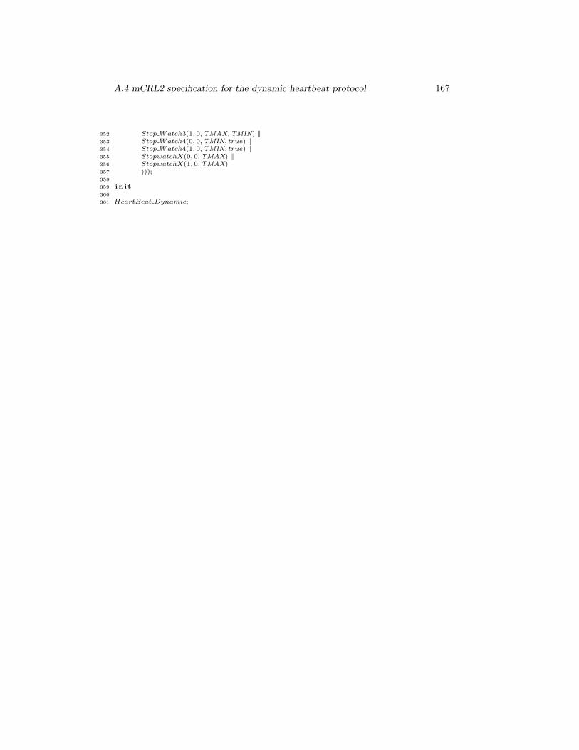
A.4 mCRL2 specification for the dynamic heartbeat protocol 167
352 Stop Watch3(1, 0,TMAX,TMIN) ‖353 Stop Watch4(0, 0,TMIN, true) ‖354 Stop Watch4(1, 0,TMIN, true) ‖355 StopwatchX(0, 0,TMAX) ‖356 StopwatchX(1, 0,TMAX)357 )));358
359 in i t360
361 HeartBeat Dynamic;

168 Appendix A. Heartbeat protocols

Appendix B
mCRL2 Specifications forConsensus Protocols
169
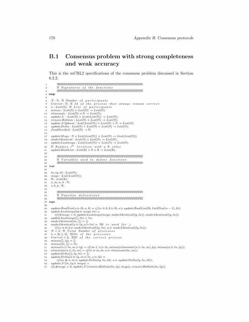
170 Appendix B. Consensus protocols
B.1 Consensus problem with strong completenessand weak accuracy
This is the mCRL2 specifications of the consensus problem discussed in Section6.2.2.
1 %%%%%%%%%%%%%%%%%%%%%%%%%%%%%%%%%%%%%%%%%%%%2 % Signatures of the funct ions3 %%%%%%%%%%%%%%%%%%%%%%%%%%%%%%%%%%%%%%%%%%%%4 map5
6 N : N; % Number of p a r t i c i p a n t s7 Correct : N; % Id of the process tha t always remain correc t8 π : List(N); % Lis t of p a r t i c i p a n t s9 minus : List(N)× List(N)→ List(N);
10 eliminate : List(N)× N→ List(N);11 update V : List(N)× List(List(N))→ List(N);12 removeBottom : List(N)× List(N)→ List(N);13 update V 2phase : List(List(N))× List(N)× N→ List(N);14 updateDelta : List(N)× List(N)× List(N)→ List(N);15 findDecided : List(N)→ N;16
17 updateMsgs : N× List(List(N))× List(N)→ List(List(N));18 makeIdentical : List(N)× List(N)→ List(N);19 updateLastmsgs : List(List(N))× List(N)→ List(N);
20 % Replace ith l o ca t ion with a B value21 updateBoolList : List(B)× N× B→ List(B);22
23 %%%%%%%%%%%%%%%%%%%%%%%%%%%%%%%%%%%%%%%%%%%%24 % Variab les used to de f ine funct ions25 %%%%%%%%%%%%%%%%%%%%%%%%%%%%%%%%%%%%%%%%%%%%26 var27
28 ln, lg, ld : List(N);29 msgs : List(List(N));30 lb : List(B);31 x,m, n, k : N;32 s, b, p : B;33
34 %%%%%%%%%%%%%%%%%%%%%%%%%%%%%%%%%%%%%%%%%%%%35 % Function d e f i n i t i o n s36 %%%%%%%%%%%%%%%%%%%%%%%%%%%%%%%%%%%%%%%%%%%%37 eqn38
39 updateBoolList(s� lb, n, b) = if(n ≈ 0, b� lb, s� updateBoolList(lb, Int2Nat(n− 1), b));40 updateLastmsgs(lg �msgs, ln) =41 if(#msgs > 0, updateLastmsgs(msgs,makeIdentical(lg, ln)),makeIdentical(lg, ln));42 updateLastmsgs([], ln) = ln;43 makeIdentical(ln, []) = [];44 makeIdentical(x� lg, n� ln) = %0 i s used for ⊥45 if(x ≈ 0, 0 �makeIdentical(lg, ln), n�makeIdentical(lg, ln));46 N = 3; % Total Number of processes47 π = [0, 1, 2]; %IDs of the processes48 Correct = 2; %ID of the correc t process49 minus([], lg) = [];50 minus(ln, []) = ln;51 minus(n� ln,m� lg) = if(m ∈ n� ln,minus(eliminate(n� ln,m), lg),minus(n� ln, lg));52 eliminate(n� ln,m) = if(n ≈ m, ln, n� eliminate(ln,m));53 updateDelta([], lg, ln) = [];54 updateDelta(n� lg,m� ln, x� ld) =55 if(m 6≈ n,m� updateDelta(lg, ln, ld), x� updateDelta(lg, ln, ld));56 update V (ln, lg �msgs) =57 if(#msgs > 0, update V (removeBottom(ln, lg),msgs), removeBottom(ln, lg));
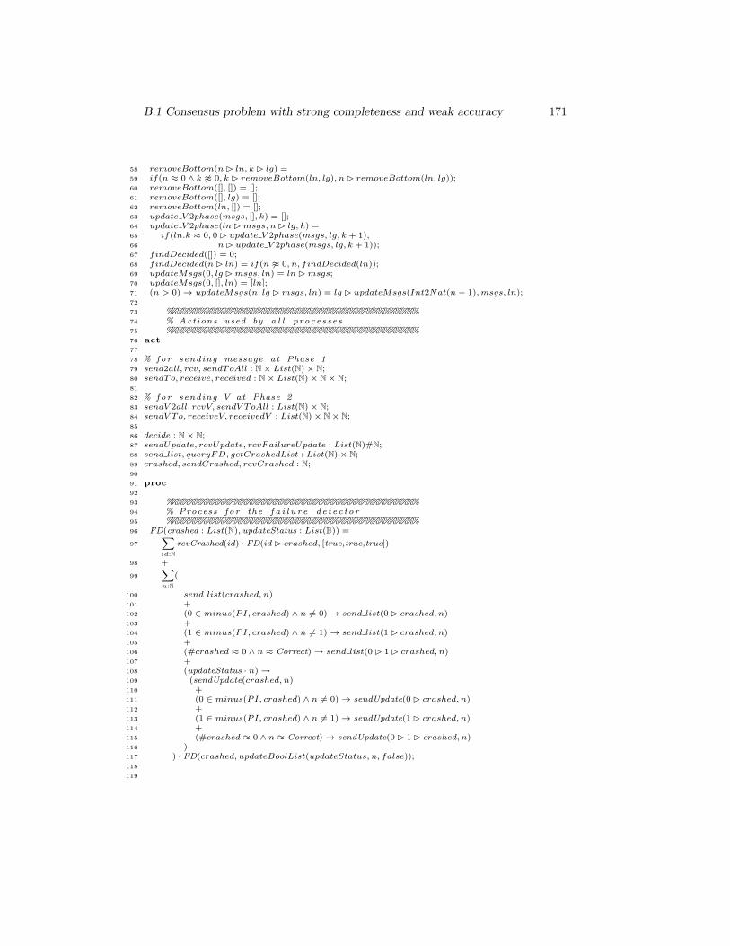
B.1 Consensus problem with strong completeness and weak accuracy 171
58 removeBottom(n� ln, k � lg) =59 if(n ≈ 0 ∧ k 6≈ 0, k � removeBottom(ln, lg), n� removeBottom(ln, lg));60 removeBottom([], []) = [];61 removeBottom([], lg) = [];62 removeBottom(ln, []) = [];63 update V 2phase(msgs, [], k) = [];64 update V 2phase(ln�msgs, n� lg, k) =65 if(ln.k ≈ 0, 0 � update V 2phase(msgs, lg, k + 1),66 n� update V 2phase(msgs, lg, k + 1));67 findDecided([]) = 0;68 findDecided(n� ln) = if(n 6≈ 0, n, findDecided(ln));69 updateMsgs(0, lg �msgs, ln) = ln�msgs;70 updateMsgs(0, [], ln) = [ln];71 (n > 0)→ updateMsgs(n, lg �msgs, ln) = lg � updateMsgs(Int2Nat(n− 1),msgs, ln);72
73 %%%%%%%%%%%%%%%%%%%%%%%%%%%%%%%%%%%%%%%%%%%%74 % Actions used by a l l processes75 %%%%%%%%%%%%%%%%%%%%%%%%%%%%%%%%%%%%%%%%%%%%76 act77
78 % for sending message at Phase 179 send2all, rcv, sendToAll : N× List(N)× N;80 sendTo, receive, received : N× List(N)× N× N;81
82 % for sending V at Phase 283 sendV 2all, rcvV, sendV ToAll : List(N)× N;84 sendV To, receiveV, receivedV : List(N)× N× N;85
86 decide : N× N;87 sendUpdate, rcvUpdate, rcvFailureUpdate : List(N)#N;88 send list, queryFD, getCrashedList : List(N)× N;89 crashed, sendCrashed, rcvCrashed : N;90
91 proc92
93 %%%%%%%%%%%%%%%%%%%%%%%%%%%%%%%%%%%%%%%%%%%%94 % Process for the f a i l u r e de tec tor95 %%%%%%%%%%%%%%%%%%%%%%%%%%%%%%%%%%%%%%%%%%%%96 FD(crashed : List(N), updateStatus : List(B)) =
97
∑id:N
rcvCrashed(id) · FD(id� crashed, [true,true,true])
98 +
99
∑n:N
(
100 send list(crashed, n)101 +102 (0 ∈ minus(PI, crashed) ∧ n 6= 0)→ send list(0 � crashed, n)103 +104 (1 ∈ minus(PI, crashed) ∧ n 6= 1)→ send list(1 � crashed, n)105 +106 (#crashed ≈ 0 ∧ n ≈ Correct)→ send list(0 � 1 � crashed, n)107 +108 (updateStatus · n)→109 (sendUpdate(crashed, n)110 +111 (0 ∈ minus(PI, crashed) ∧ n 6= 0)→ sendUpdate(0 � crashed, n)112 +113 (1 ∈ minus(PI, crashed) ∧ n 6= 1)→ sendUpdate(1 � crashed, n)114 +115 (#crashed ≈ 0 ∧ n ≈ Correct)→ sendUpdate(0 � 1 � crashed, n)116 )117 ) · FD(crashed, updateBoolList(updateStatus, n, false));118
119
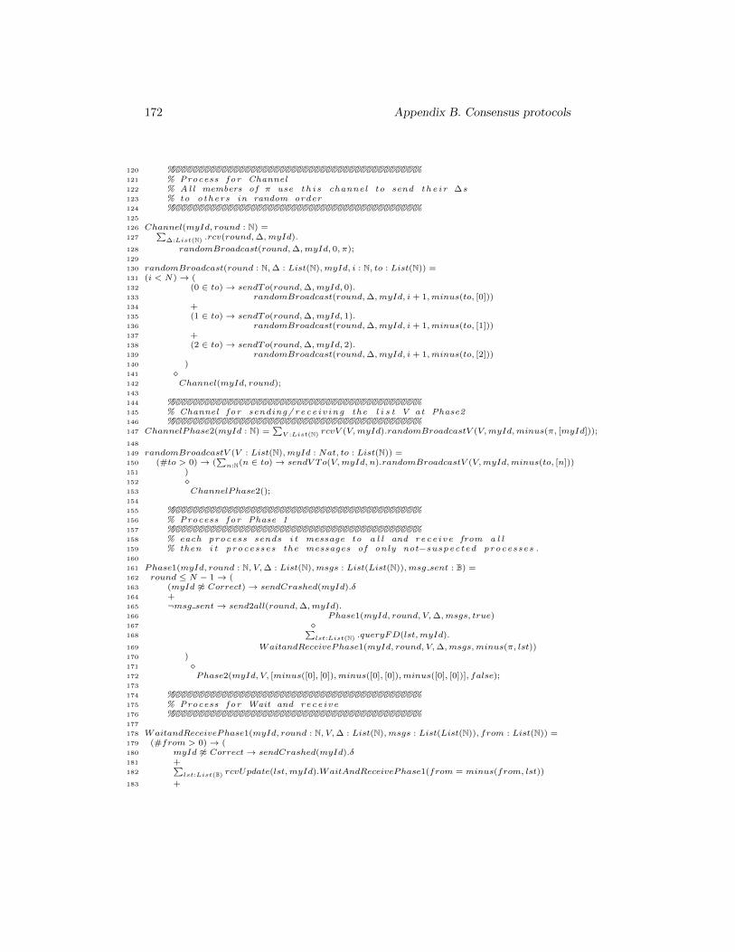
172 Appendix B. Consensus protocols
120 %%%%%%%%%%%%%%%%%%%%%%%%%%%%%%%%%%%%%%%%%%%%121 % Process for Channel122 % Al l members of π use t h i s channel to send t h e i r ∆s123 % to others in random order124 %%%%%%%%%%%%%%%%%%%%%%%%%%%%%%%%%%%%%%%%%%%%125
126 Channel(myId, round : N) =127
∑∆:List(N) .rcv(round,∆,myId).
128 randomBroadcast(round,∆,myId, 0, π);129
130 randomBroadcast(round : N,∆ : List(N),myId, i : N, to : List(N)) =131 (i < N)→ (132 (0 ∈ to)→ sendTo(round,∆,myId, 0).133 randomBroadcast(round,∆,myId, i+ 1,minus(to, [0]))134 +135 (1 ∈ to)→ sendTo(round,∆,myId, 1).136 randomBroadcast(round,∆,myId, i+ 1,minus(to, [1]))137 +138 (2 ∈ to)→ sendTo(round,∆,myId, 2).139 randomBroadcast(round,∆,myId, i+ 1,minus(to, [2]))140 )141 �142 Channel(myId, round);143
144 %%%%%%%%%%%%%%%%%%%%%%%%%%%%%%%%%%%%%%%%%%%%145 % Channel for sending / rece i v ing the l i s t V at Phase2146 %%%%%%%%%%%%%%%%%%%%%%%%%%%%%%%%%%%%%%%%%%%%147 ChannelPhase2(myId : N) =
∑V :List(N) rcvV (V,myId).randomBroadcastV (V,myId,minus(π, [myId]));
148
149 randomBroadcastV (V : List(N),myId : Nat, to : List(N)) =150 (#to > 0)→ (
∑n:N(n ∈ to)→ sendV To(V,myId, n).randomBroadcastV (V,myId,minus(to, [n]))
151 )152 �153 ChannelPhase2();154
155 %%%%%%%%%%%%%%%%%%%%%%%%%%%%%%%%%%%%%%%%%%%%156 % Process for Phase 1157 %%%%%%%%%%%%%%%%%%%%%%%%%%%%%%%%%%%%%%%%%%%%158 % each process sends i t message to a l l and rece ive from a l l159 % then i t processes the messages of only not−suspected processes .160
161 Phase1(myId, round : N, V,∆ : List(N),msgs : List(List(N)),msg sent : B) =162 round ≤ N − 1→ (163 (myId 6≈ Correct)→ sendCrashed(myId).δ164 +165 ¬msg sent→ send2all(round,∆,myId).166 Phase1(myId, round, V,∆,msgs, true)167 �168
∑lst:List(N) .queryFD(lst,myId).
169 WaitandReceivePhase1(myId, round, V,∆,msgs,minus(π, lst))170 )171 �172 Phase2(myId, V, [minus([0], [0]),minus([0], [0]),minus([0], [0])], false);173
174 %%%%%%%%%%%%%%%%%%%%%%%%%%%%%%%%%%%%%%%%%%%%175 % Process for Wait and rece ive176 %%%%%%%%%%%%%%%%%%%%%%%%%%%%%%%%%%%%%%%%%%%%177
178 WaitandReceivePhase1(myId, round : N, V,∆ : List(N),msgs : List(List(N)), from : List(N)) =179 (#from > 0)→ (180 myId 6≈ Correct→ sendCrashed(myId).δ181 +182
∑lst:List(B) rcvUpdate(lst,myId).WaitAndReceivePhase1(from = minus(from, lst))
183 +
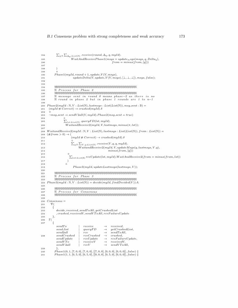
B.1 Consensus problem with strong completeness and weak accuracy 173
184∑
q:N∑
∆q :List(N) .receive(round,∆q, q,myId).
185 WaitAndReceivePhase1(msgs = updatemsgs(msgs, q,Deltaq),186 from = minus(from, [q]))187
188 )189 �190 Phase1(myId, round+ 1, update V (V,msgs),191 updateDelta(V, update V (V,msgs), [⊥,⊥,⊥]),msgs, false);192
193
194 %%%%%%%%%%%%%%%%%%%%%%%%%%%%%%%%%%%%%%%%%%%%195 % Process for Phase 2196 %%%%%%%%%%%%%%%%%%%%%%%%%%%%%%%%%%%%%%%%%%%%197 % message sent in round 0 means phase−2 as there i s no198 % round in phase 2 but in phase 1 rounds are 1 to n−1199
200 Phase2(myId : N, V : List(N), lastmsgs : List(List(N)),msg sent : B) =201 (myId 6≈ Correct)→ crashed(myId).δ202 +203 ¬msg sent→ sendV 2all(V,myId).Phase2(msg sent = true)204 �205
∑lst:List(N) .queryFD(lst,myId).
206 WaitandReceive2(myId, V, lastmsgs,minus(π, lst));207
208 WaitandReceive2(myId : N, V : List(N), lastmsgs : List(List(N)), from : List(N)) =209 (#from > 0)→ (210 (myId 6≈ Correct)→ crashed(myId).δ211 +212
∑q:N
∑V q:List(N) .receive(V q, q,myId).
213 WaitandReceive2(myId, V, updateMsgs(q, lastmsgs, V q),214 minus(from, [q]))215 +216
∑lst:List(B) rcvUpdate(lst,myId).WaitAndReceive2(from = minus(from, lst))
217 )218 �219 Phase3(myId, updateLastmsgs(lastmsgs, V ));220
221 %%%%%%%%%%%%%%%%%%%%%%%%%%%%%%%%%%%%%%%%%%%%222 % Process for Phase 3223 %%%%%%%%%%%%%%%%%%%%%%%%%%%%%%%%%%%%%%%%%%%%224 Phase3(myId : N, V : List(N)) = decide(myId, findDecided(V )).δ;225
226 %%%%%%%%%%%%%%%%%%%%%%%%%%%%%%%%%%%%%%%%%%%%227 % Process for Consensus228 %%%%%%%%%%%%%%%%%%%%%%%%%%%%%%%%%%%%%%%%%%%%229
230 Consensus =231 ∇(232 {233 decide, received, sendToAll, getCrashedList234 , crashed, receivedV, sendV ToAll, rcvFailureUpdate235 },236 Γ(237 {
238
sendTo | receive → received,send list | queryFD → getCrashedList,send2all | rcv → sendToAll,sendCrashed | rcvCrashed → crashed,sendUpdate | rcvUpdate → rcvFailureUpdate,sendV To | receiveV → receivedV,sendV 2all | rcvV → sendV ToAll,
239 },240 Phase1(0, 1, [7, 0, 0], [7, 0, 0], [[7, 0, 0], [0, 0, 0], [0, 0, 0]], false) ‖241 Phase1(1, 1, [0, 5, 0], [0, 5, 0], [[0, 0, 0], [0, 5, 0], [0, 0, 0]], false) ‖
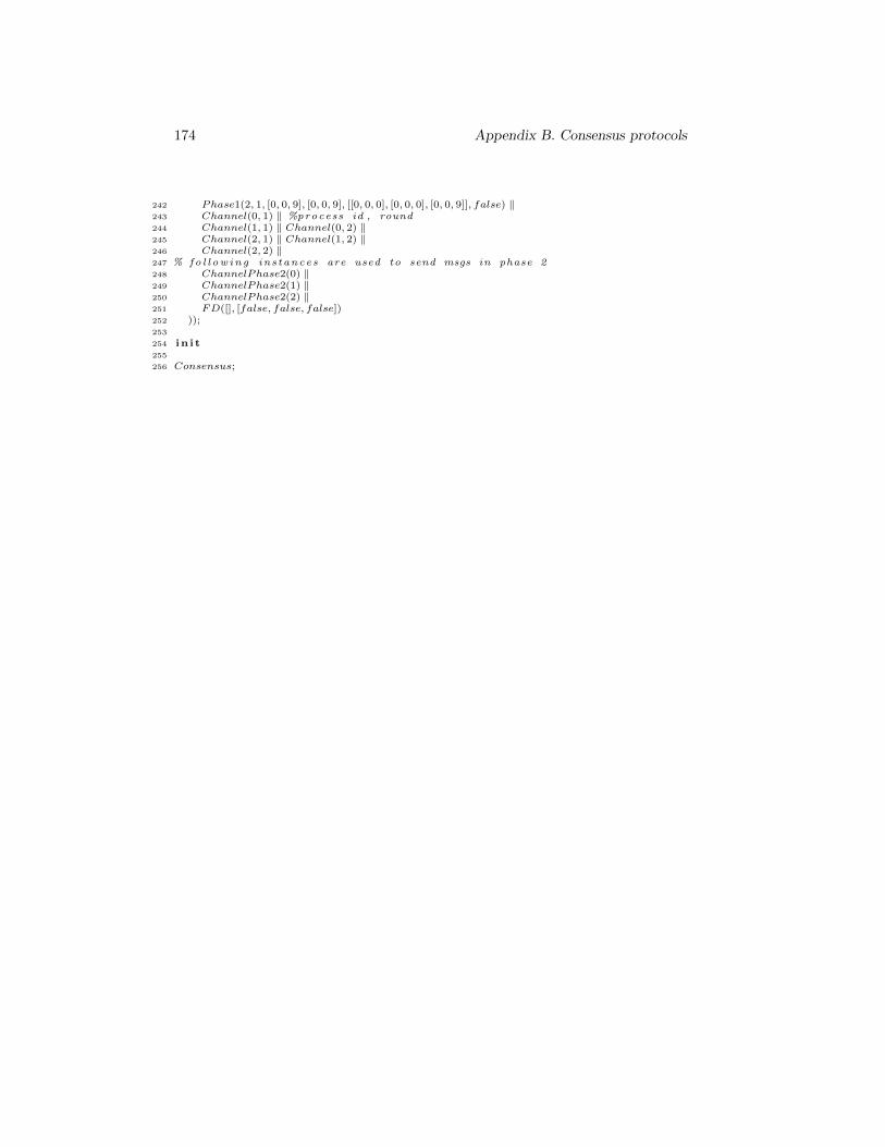
174 Appendix B. Consensus protocols
242 Phase1(2, 1, [0, 0, 9], [0, 0, 9], [[0, 0, 0], [0, 0, 0], [0, 0, 9]], false) ‖243 Channel(0, 1) ‖ %process id , round244 Channel(1, 1) ‖ Channel(0, 2) ‖245 Channel(2, 1) ‖ Channel(1, 2) ‖246 Channel(2, 2) ‖247 % f o l l o w i n g ins tances are used to send msgs in phase 2248 ChannelPhase2(0) ‖249 ChannelPhase2(1) ‖250 ChannelPhase2(2) ‖251 FD([], [false, false, false])252 ));253
254 in i t255
256 Consensus;
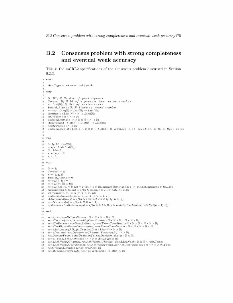
B.2 Consensus problem with strong completeness and eventual weak accuracy175
B.2 Consensus problem with strong completenessand eventual weak accuracy
This is the mCRL2 specifications of the consensus problem discussed in Section6.2.3.
1 sort2
3 Ack Type = struct ack | nack;4
5 map6
7 N : N+; % Number of p a r t i c i p a n t s8 Correct : N; % Id of a process tha t never crashes9 π : List(N); % Set of p a r t i c i p a n t s
10 Initial Round : N; % Star t ing round number11 minus : List(N)× List(N)→ List(N);12 eliminate : List(N)× N→ List(N);13 isGreater : N× N→ N;14 updateEstimate : N× N× N× N→ N;15 Addcrashed : List(N)× List(N)→ List(N);16 nextProcess : N→ N;17 updateBoolList : List(B)× N× B→ List(B); % Replace i ˆ th loca t ion with a Bool va lue18
19
20 var21
22 ln, lg, ld : List(N);23 msgs : List(List(N));24 lb : List(B);25 x,m, n, k : N;26 s, b : B;27
28 eqn29
30 N = 3;31 Correct = 2;32 π = [1, 2, 3];33 Initial Round = 0;34 minus([], lg) = [];35 minus(ln, []) = ln;36 minus(n� ln,m� lg) = if(m ∈ n� ln,minus(eliminate(n� ln,m), lg),minus(n� ln, lg));37 eliminate(n� ln,m) = if(n ≈ m, ln, n� eliminate(ln,m));38 isGreater(n,m) = if(m > n,m, n);39 updateEstimate(x, k, n,m) = if(m > n, k, x);40 Addcrashed(n, lg) = if(n ≈ Correct ∨ n ∈ lg, lg, n� lg);41 nextProcess(n) = if(n ≈ 2, 0, n+ 1);42 updateBoolList(s� lb, n, b) = if(n ≈ 0, b� lb, s� updateBoolList(lb, Int2Nat(n− 1), b));43
44 act45
46 send, rcv, send2Coordinator : N× N× N× N× N;47 sendTo, rcvfrom, receivedByCoordinator : N× N× N× N× N× N;48 sendToProcess, rcvNewEstimate, rcvdFromCoordinatorN× N× N× N× N× N;49 sendToAll, rcvFromCoordinator, sentFromCoordinator : N× N× N× N× N;50 send list, queryFD, getCrashedList : List(N)× N× N;51 sendDecision, rcvDecisionatChannel,DecisionBC : N× N;52 rcvDecisioFrom, sendDecisionTo, rcvDecision, decide : N× N;53 send3, rcv3, SendAckNack : N× N× Ack Type× N;54 sendAckNack2Channel, rcvAckNackatChannel, SendAckNack : N× N× Ack Type;55 sendAckNack2Coordinator, rcvAckNackFromChannel, RcvAckNack : N× N× Ack Type;56 rcvCrashed, sendCrashed, crashed : N;57 sendUpdate, rcvUpdate, rcvFailureUpdate : List(N)× N;
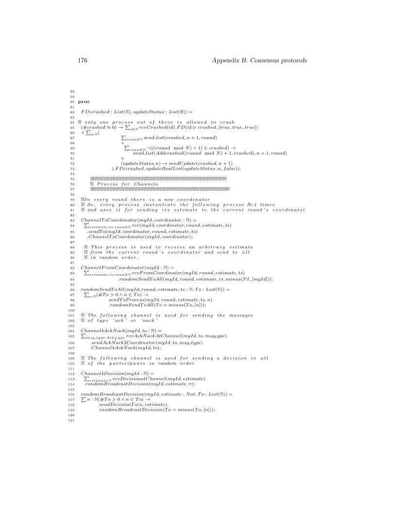
176 Appendix B. Consensus protocols
58
59
60 proc61
62 FD(crashed : List(N), updateStatus : List(B)) =63
64 % only one process out of three i s a l lowed to crash65 (#crashed ≈ 0)→∑
id:N rcvCrashed(id).FD(id� crashed, [true, true, true])66 +
∑n:N(
67∑
round:N send list(crashed, n+ 1, round)68 +69
∑round:N ¬(((round mod N) + 1) ∈ crashed)→
70 send list(Addcrashed((round mod N) + 1, crashed), n+ 1, round)71 +72 (updateStatus.n)→ sendUpdate(crashed, n+ 1)73 ).FD(crashed, updateBoolList(updateStatus, n, false));74
75 %%%%%%%%%%%%%%%%%%%%%%%%%%%%%%%%%%%%%%%%%%%%76 % Process for Channels77 %%%%%%%%%%%%%%%%%%%%%%%%%%%%%%%%%%%%%%%%%%%%%78
79 %In every round there i s a new coordinator80 % So , every process i n s t a n t i a t e the f o l l o w i n g process N−1 times81 % and uses i t for sending i t s est imate to the current round ’ s coordinator82
83 ChannelToCoordonator(myId, coordinator : N) =84
∑estimate,ts,round:N rcv(myId, coordinator, round, estimate, ts)
85 .sendTo(myId, coordinator, round, estimate, ts)86 .ChannelToCoordonator(myId, coordinator);87
88 % This process i s used to rece ive an a r b i t r a r y est imate89 % from the current round ’ s coordinator and send to a l l90 % in random order .91
92 ChannelFromCoordonator(myId : N) =93
∑estimate,ts,round:N rcvFromCoordinator(myId, round, estimate, ts)
94 .randomSendToAll(myId, round, estimate, ts,minus(PI, [myId]));95
96 randomSendToAll(myId, round, estimate, ts : N, To : List(N)) =97
∑n:N(#To > 0 ∧ n ∈ To)→
98 sendToProcess(myId, round, estimate, ts, n)99 .randomSendToAll(To = minus(To, [n]));
100
101 % The f o l l o w i n g channel i s used for sending the messages102 % of type ‘ ack ’ or ‘ nack ’103
104 Channel4AckNack(myId, to : N) =105
∑msg type:AckT ype rcvAckNackAtChannel(myId, to,msgtype)
106 .sendAckNack2Coordinator(myId, to,msg type)107 .Channel4AckNack(myId, to);108
109 % The f o l l o w i n g channel i s used for sending a dec i s ion to a l l110 % of the p a r t i c i p a n t s in random order111
112 Channel4Decision(myId : N) =113
∑estimate:N rcvDecisionatChannel(myId, estimate)
114 .randomBroadcastDecision(myId, estimate, π);115
116 randomBroadcastDecision(myId, estimate : Nat, To : List(N)) =117
∑n : N(#To > 0 ∧ n ∈ To)→
118 sendDecisionTo(n, estimate).119 randomBroadcastDecision(To = minus(To, [n]));120
121
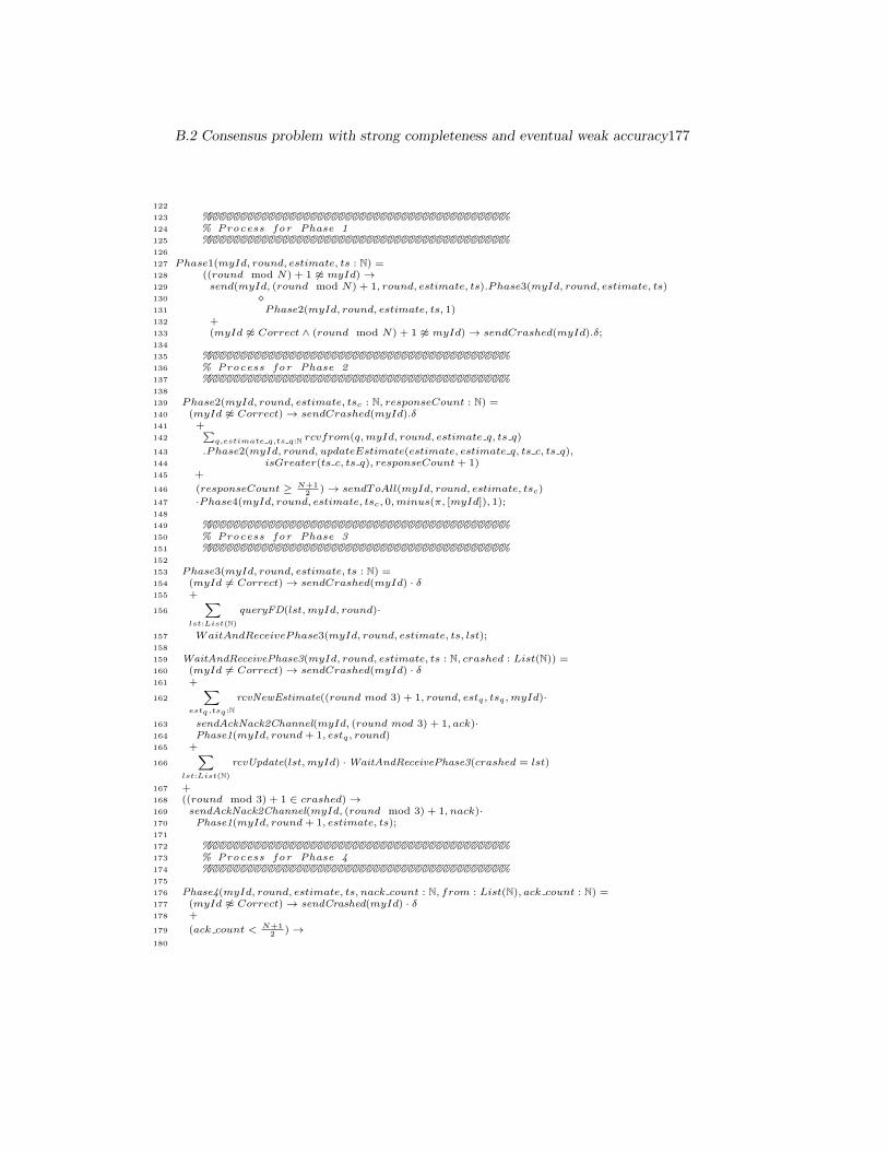
B.2 Consensus problem with strong completeness and eventual weak accuracy177
122
123 %%%%%%%%%%%%%%%%%%%%%%%%%%%%%%%%%%%%%%%%%%%%124 % Process for Phase 1125 %%%%%%%%%%%%%%%%%%%%%%%%%%%%%%%%%%%%%%%%%%%%126
127 Phase1(myId, round, estimate, ts : N) =128 ((round mod N) + 1 6≈ myId)→129 send(myId, (round mod N) + 1, round, estimate, ts).Phase3(myId, round, estimate, ts)130 �131 Phase2(myId, round, estimate, ts, 1)132 +133 (myId 6≈ Correct ∧ (round mod N) + 1 6≈ myId)→ sendCrashed(myId).δ;134
135 %%%%%%%%%%%%%%%%%%%%%%%%%%%%%%%%%%%%%%%%%%%%136 % Process for Phase 2137 %%%%%%%%%%%%%%%%%%%%%%%%%%%%%%%%%%%%%%%%%%%%138
139 Phase2(myId, round, estimate, tsc : N, responseCount : N) =140 (myId 6≈ Correct)→ sendCrashed(myId).δ141 +142
∑q,estimate q,ts q:N rcvfrom(q,myId, round, estimate q, ts q)
143 .Phase2(myId, round, updateEstimate(estimate, estimate q, ts c, ts q),144 isGreater(ts c, ts q), responseCount+ 1)145 +
146 (responseCount ≥ N+12 )→ sendToAll(myId, round, estimate, tsc)
147 ·Phase4(myId, round, estimate, tsc, 0,minus(π, [myId]), 1);148
149 %%%%%%%%%%%%%%%%%%%%%%%%%%%%%%%%%%%%%%%%%%%%150 % Process for Phase 3151 %%%%%%%%%%%%%%%%%%%%%%%%%%%%%%%%%%%%%%%%%%%%152
153 Phase3(myId, round, estimate, ts : N) =154 (myId 6= Correct)→ sendCrashed(myId) · δ155 +
156
∑lst:List(N)
queryFD(lst,myId, round)·
157 WaitAndReceivePhase3(myId, round, estimate, ts, lst);158
159 WaitAndReceivePhase3(myId, round, estimate, ts : N, crashed : List(N)) =160 (myId 6= Correct)→ sendCrashed(myId) · δ161 +
162
∑estq,tsq :N
rcvNewEstimate((round mod 3) + 1, round, estq, tsq,myId)·
163 sendAckNack2Channel(myId, (round mod 3) + 1, ack)·164 Phase1(myId, round+ 1, estq, round)165 +
166
∑lst:List(N)
rcvUpdate(lst,myId) ·WaitAndReceivePhase3(crashed = lst)
167 +168 ((round mod 3) + 1 ∈ crashed)→169 sendAckNack2Channel(myId, (round mod 3) + 1, nack)·170 Phase1(myId, round+ 1, estimate, ts);171
172 %%%%%%%%%%%%%%%%%%%%%%%%%%%%%%%%%%%%%%%%%%%%173 % Process for Phase 4174 %%%%%%%%%%%%%%%%%%%%%%%%%%%%%%%%%%%%%%%%%%%%175
176 Phase4(myId, round, estimate, ts, nack count : N, from : List(N), ack count : N) =177 (myId 6≈ Correct)→ sendCrashed(myId) · δ178 +
179 (ack count < N+12 )→
180
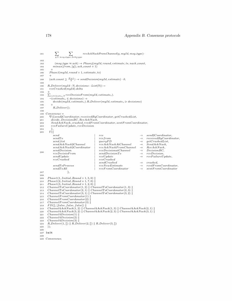
178 Appendix B. Consensus protocols
181
∑q:N
∑msg type:AckT ype
rcvAckNackFromChannel(q,myId,msg type)·
182
183 (msg type ≈ ack)→ Phase4(myId, round, estimate, ts, nack count,184 minus(from, [q]), ack count+ 1)185 �186 Phase1(myId, round+ 1, estimate, ts)187 +
188 (ack count ≥ N+12 )→ sendDecision(myId, estimate) · δ;
189
190 R Deliver(myId : N, decisions : List(N)) =191 rcvCrashed(myId).delta192 +193
∑estimatec:N rcvDecisioFrom(myId, estimatec).
194 ¬(estimatec ∈ decisions)→195 decide(myId, estimatec).R Deliver(myId, estimatec � decisions)196 �197 R Deliver();198
199 Consensus =200 ∇({send2Coordinator, receivedByCoordinator, getCrashedList,201 decide,DecisionBC,RcvAckNack,202 SendAckNack, crashed, rcvdFromCoordinator, sentFromCoordinator,203 rcvFailureUpdate, rcvDecision204 },205 Γ({
206
send | rcv → send2Coordinator,sendTo | rcvfrom → receivedByCoordinator,send list | queryFD → getCrashedList,sendAckNack2Channel | rcvAckNackAtChannel → SendAckNack,sendAckNack2Coordinator | rcvAckNackFromChannel → RcvAckNack,sendDecision | rcvDecisionatChannel → DecisionBC,rcvDecisioFrom | sendDecisionTo → rcvDecision,sendUpdate | rcvUpdate → rcvFailureUpdate,rcvCrashed | rcvCrashed
| sendCrashed → crashed,sendToProcess | rcvNewEstimate → rcvdFromCoordinator,sendToAll | rcvFromCoordinator → sentFromCoordinator
207 },208
209 Phase1(1, Initial Round+ 1, 5, 0) ‖210 Phase1(2, Initial Round+ 1, 7, 0) ‖211 Phase1(3, Initial Round+ 1, 2, 0) ‖212 ChannelToCoordonator(1, 2) ‖ ChannelToCoordonator(1, 3) ‖213 ChannelToCoordonator(2, 1) ‖ ChannelToCoordonator(2, 3) ‖214 ChannelToCoordonator(3, 1) ‖ ChannelToCoordonator(3, 2) ‖215 ChannelFromCoordonator(1) ‖216 ChannelFromCoordonator(2) ‖217 ChannelFromCoordonator(3) ‖218 FD([], [false, false, false]) ‖219 Channel4AckNack(1, 2) ‖ Channel4AckNack(1, 3) ‖ Channel4AckNack(2, 1) ‖220 Channel4AckNack(3, 2) ‖ Channel4AckNack(2, 3) ‖ Channel4AckNack(3, 1) ‖221 Channel4Decision(1) ‖222 Channel4Decision(2) ‖223 Channel4Decision(3) ‖224 R Deliver(1, []) ‖ R Deliver(2, []) ‖ R Deliver(3, [])225 ));226
227 in i t228
229 Consensus;
Appendix C
mCRL2 Specifications forMembership Protocols
179
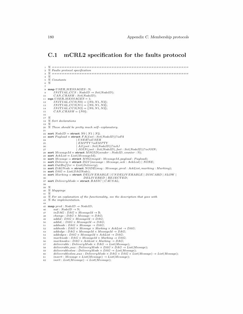
180 Appendix C. Membership protocols
C.1 mCRL2 specification for the faults protocol
1 % =======================================================2 % Faults protocol specification3 % =======================================================4 %5 % Constants6 %7
8 map USER MESSAGES : N;9 INITIAL CCS : NodeID → Set(NodeID);
10 CAN CRASH : Set(NodeID);11 eqn USER MESSAGES = 1;12 INITIAL CCS(N0) = {N0, N1, N2};13 INITIAL CCS(N1) = {N0, N1, N2};14 INITIAL CCS(N2) = {N0, N1, N2};15 CAN CRASH = {N0};16
17 %18 % Sort declarations19 %20 % These should be pretty much self−explanatory.21
22 sort NodeID = struct N0 | N1 | N2;23 sort Payload = struct FA(fset : Set(NodeID))?isFA24 | USER?isUSER25 | EMPTY ?isEMPTY26 | AJ(jset : Set(NodeID))?isAJ27 | JOIN(jset : Set(NodeID), fset : Set(NodeID))?isJOIN ;28 sort MessageId = struct MSGID(sender : NodeID, counter : N);29 sort AckList = List(MessageId);30 sort Message = struct MSG(msgid : MessageId, payload : Payload);31 sort Delivery = struct DLV (message : Message, ack : AckList) | NONE ;32 sort OutBuffer = List(Delivery);33 sort DAGNode = struct NODE(msg : Message, pred : AckList,marking : Marking);34 sort DAG = List(DAGNode);35 sort Marking = struct DELIV ERABLE | UNDELIV ERABLE | DISCARD | SLOW |36 DELIV ERED | REJECTED;37 sort DeliveryMode = struct BASIC | CAUSAL;38
39 %40 % Mappings41 %42 % For an explanation of the functionality, see the description that goes with43 % the implementation.44
45 map pred : NodeID → NodeID;46 nat : NodeID → N;47 inDAG : DAG ×MessageId → B;48 change : DAG ×Message → DAG;49 addid : DAG ×MessageId → DAG;50 addid : DAG ×MessageId → DAG;51 addnode : DAG ×Message → DAG;52 addnode : DAG ×Message ×Marking × AckList → DAG;53 addedge : DAG ×MessageId ×MessageId → DAG;54 addedges : DAG ×MessageId × AckList → DAG;55 marknode : DAG ×MessageId ×Marking → DAG;56 marknodes : DAG × AckList ×Marking → DAG;57 deliverable : DeliveryMode×DAG → List(Message);58 deliverable aux : DeliveryMode×DAG ×DAG → List(Message);59 deliverableslow : DeliveryMode×DAG → List(Message);60 deliverableslow aux : DeliveryMode×DAG ×DAG × List(Message)→ List(Message);61 insert : Message× List(Message)→ List(Message);62 isort : List(Message)→ List(Message);
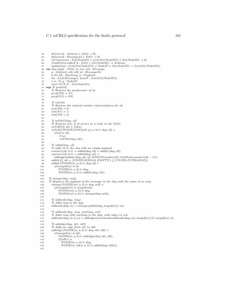
C.1 mCRL2 specification for the faults protocol 181
63 delivered : AckList×DAG → B;64 delivered : MessageId×DAG → B;65 isConsensus : Set(NodeID)× List(Set(NodeID))× Set(NodeID)→ B;66 findDeliverableFA : DAG × Set(NodeID)→ AckList;67 updatelast : List(Set(NodeID))× NodeID × Set(NodeID)→ List(Set(NodeID));68 var dag, dag1 : DAG; m,m1,m2 : Message;69 a : AckList; id1, id2, id : MessageId;70 k, k1, k2 : Marking; p : Payload;71 lm : List(Message); LastF : List(Set(NodeID));72 r, n : N; q : NodeID;73 fset, CCS, F : Set(NodeID);74 eqn % pred(id)75 % Returns the predecessor of id.76 pred(N2) = N1;77 pred(N1) = N0;78
79 % nat(id)80 % Returns the natural number representation for id.81 nat(N0) = 0;82 nat(N1) = 1;83 nat(N2) = 2;84
85 % inDAG(dag, id)86 % Returns true if id occurs as a node in the DAG.87 inDAG([], id) = false;88 inDAG(NODE(MSG(id1, p), a, k) � dag, id) =89 if(id ≈ id1,90 true,91 inDAG(dag, id));92
93 % addid(dag, id)94 % adds id to the dag with an empty payload95 counter(id) ≈ 0→ addid(dag, id) = addid (dag, id);96 counter(id) 6= 0→ addid(dag, id) =97 addedge(addid (dag, id), id,MSGID(sender(id), Int2Nat(counter(id)− 1)));98 addid ([], id) = [NODE(MSG(id, EMPTY ), [], UNDELIV ERABLE)];99 addid (NODE(m, a, k) � dag, id) =
100 if(msgid(m) ≈ id,101 NODE(m, a, k) � dag,102 NODE(m, a, k) � addid (dag, id));103
104 % change(dag, msg)105 % Replaces the payload of the message in the dag with the same id as msg.106 change(NODE(m1, a, k) � dag,m2) =107 if(msgid(m1) ≈ msgid(m2),108 NODE(m2, a, k) � dag,109 NODE(m1, a, k) � change(dag,m2));110
111 % addnode(dag, msg)112 % Adds msg to the dag.113 addnode(dag,m) = change(addid(dag,msgid(m)),m);114
115 % addnode(dag, msg, marking, ack)116 % Adds msg with marking to the dag, with edges to ack.117 addnode(dag,m, k, a) = addedges(marknode(addnode(dag,m),msgid(m), k),msgid(m), a);118
119 % addedge(dag, id1, id2)120 % Adds an edge from id1 to id2.121 addedge(NODE(m, a, k) � dag, id1, id2) =122 if(msgid(m) 6= id1,123 NODE(m, a, k) � addedge(dag, id1, id2),124 if(id2 ∈ a,125 NODE(m, a, k) � dag,126 NODE(m, id2 � a, k) � addid(dag, id2)));127
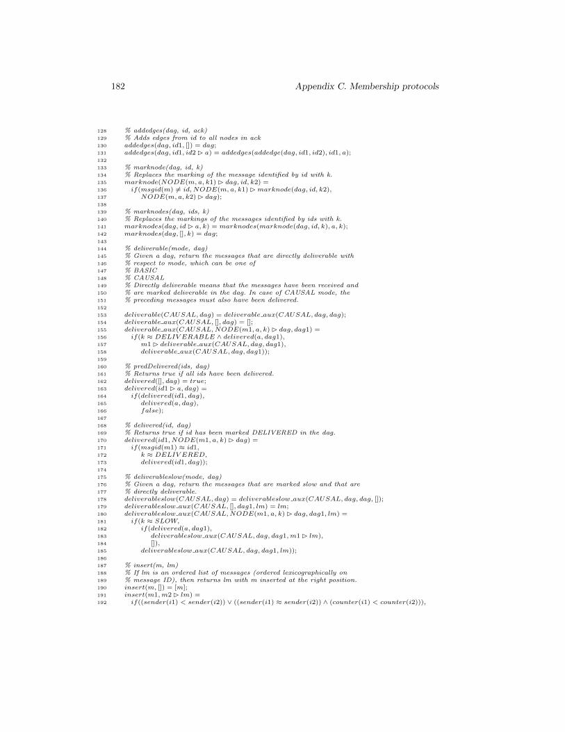
182 Appendix C. Membership protocols
128 % addedges(dag, id, ack)129 % Adds edges from id to all nodes in ack130 addedges(dag, id1, []) = dag;131 addedges(dag, id1, id2 � a) = addedges(addedge(dag, id1, id2), id1, a);132
133 % marknode(dag, id, k)134 % Replaces the marking of the message identified by id with k.135 marknode(NODE(m, a, k1) � dag, id, k2) =136 if(msgid(m) 6= id,NODE(m, a, k1) �marknode(dag, id, k2),137 NODE(m, a, k2) � dag);138
139 % marknodes(dag, ids, k)140 % Replaces the markings of the messages identified by ids with k.141 marknodes(dag, id� a, k) = marknodes(marknode(dag, id, k), a, k);142 marknodes(dag, [], k) = dag;143
144 % deliverable(mode, dag)145 % Given a dag, return the messages that are directly deliverable with146 % respect to mode, which can be one of147 % BASIC148 % CAUSAL149 % Directly deliverable means that the messages have been received and150 % are marked deliverable in the dag. In case of CAUSAL mode, the151 % preceding messages must also have been delivered.152
153 deliverable(CAUSAL, dag) = deliverable aux(CAUSAL, dag, dag);154 deliverable aux(CAUSAL, [], dag) = [];155 deliverable aux(CAUSAL,NODE(m1, a, k) � dag, dag1) =156 if(k ≈ DELIV ERABLE ∧ delivered(a, dag1),157 m1 � deliverable aux(CAUSAL, dag, dag1),158 deliverable aux(CAUSAL, dag, dag1));159
160 % predDelivered(ids, dag)161 % Returns true if all ids have been delivered.162 delivered([], dag) = true;163 delivered(id1 � a, dag) =164 if(delivered(id1, dag),165 delivered(a, dag),166 false);167
168 % delivered(id, dag)169 % Returns true if id has been marked DELIVERED in the dag.170 delivered(id1, NODE(m1, a, k) � dag) =171 if(msgid(m1) ≈ id1,172 k ≈ DELIV ERED,173 delivered(id1, dag));174
175 % deliverableslow(mode, dag)176 % Given a dag, return the messages that are marked slow and that are177 % directly deliverable.178 deliverableslow(CAUSAL, dag) = deliverableslow aux(CAUSAL, dag, dag, []);179 deliverableslow aux(CAUSAL, [], dag1, lm) = lm;180 deliverableslow aux(CAUSAL,NODE(m1, a, k) � dag, dag1, lm) =181 if(k ≈ SLOW,182 if(delivered(a, dag1),183 deliverableslow aux(CAUSAL, dag, dag1,m1 � lm),184 []),185 deliverableslow aux(CAUSAL, dag, dag1, lm));186
187 % insert(m, lm)188 % If lm is an ordered list of messages (ordered lexicographically on189 % message ID), then returns lm with m inserted at the right position.190 insert(m, []) = [m];191 insert(m1,m2 � lm) =192 if((sender(i1) < sender(i2)) ∨ ((sender(i1) ≈ sender(i2)) ∧ (counter(i1) < counter(i2))),
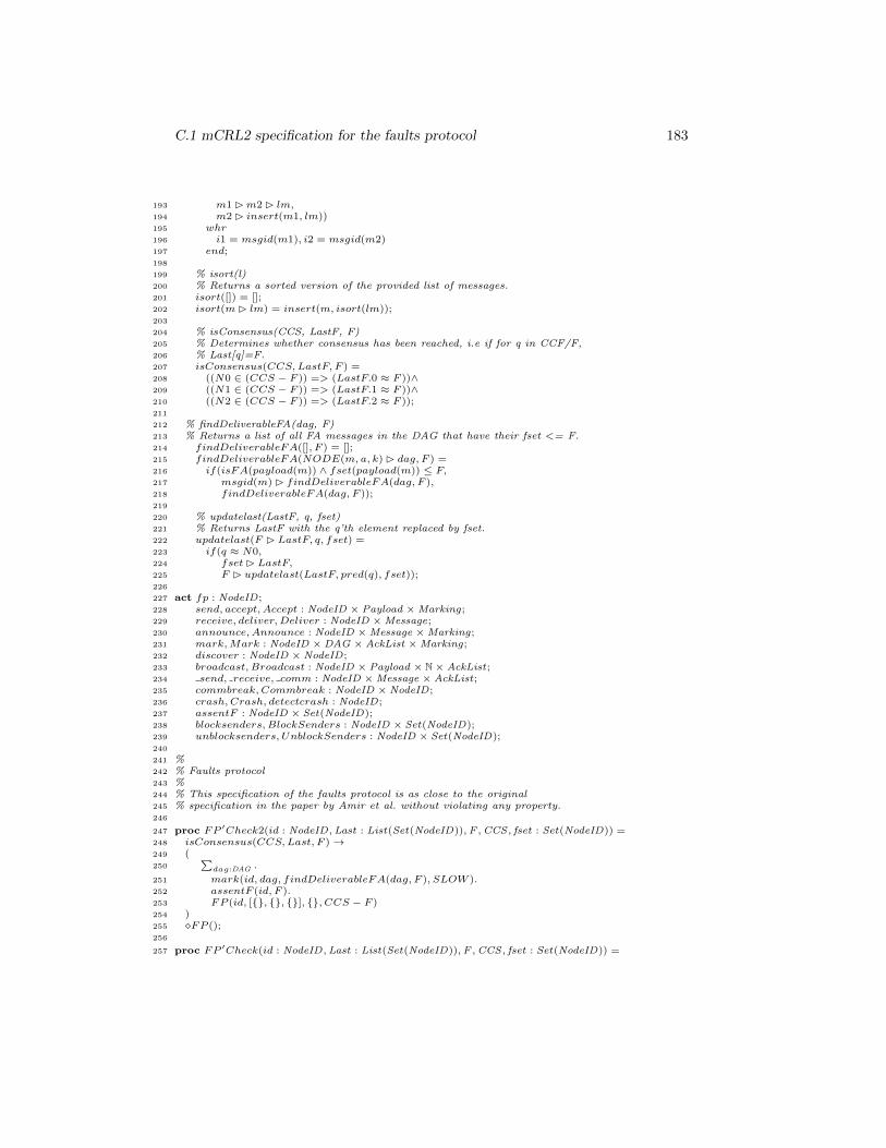
C.1 mCRL2 specification for the faults protocol 183
193 m1 �m2 � lm,194 m2 � insert(m1, lm))195 whr196 i1 = msgid(m1), i2 = msgid(m2)197 end;198
199 % isort(l)200 % Returns a sorted version of the provided list of messages.201 isort([]) = [];202 isort(m� lm) = insert(m, isort(lm));203
204 % isConsensus(CCS, LastF, F)205 % Determines whether consensus has been reached, i.e if for q in CCF/F,206 % Last[q]=F.207 isConsensus(CCS,LastF, F ) =208 ((N0 ∈ (CCS − F )) => (LastF.0 ≈ F ))∧209 ((N1 ∈ (CCS − F )) => (LastF.1 ≈ F ))∧210 ((N2 ∈ (CCS − F )) => (LastF.2 ≈ F ));211
212 % findDeliverableFA(dag, F)213 % Returns a list of all FA messages in the DAG that have their fset <= F.214 findDeliverableFA([], F ) = [];215 findDeliverableFA(NODE(m, a, k) � dag, F ) =216 if(isFA(payload(m)) ∧ fset(payload(m)) ≤ F,217 msgid(m) � findDeliverableFA(dag, F ),218 findDeliverableFA(dag, F ));219
220 % updatelast(LastF, q, fset)221 % Returns LastF with the q’th element replaced by fset.222 updatelast(F � LastF, q, fset) =223 if(q ≈ N0,224 fset� LastF,225 F � updatelast(LastF, pred(q), fset));226
227 act fp : NodeID;228 send, accept, Accept : NodeID × Payload ×Marking;229 receive, deliver,Deliver : NodeID ×Message;230 announce,Announce : NodeID ×Message ×Marking;231 mark,Mark : NodeID ×DAG × AckList ×Marking;232 discover : NodeID × NodeID;233 broadcast, Broadcast : NodeID × Payload × N× AckList;234 send, receive, comm : NodeID ×Message × AckList;235 commbreak, Commbreak : NodeID × NodeID;236 crash, Crash, detectcrash : NodeID;237 assentF : NodeID × Set(NodeID);238 blocksenders,BlockSenders : NodeID × Set(NodeID);239 unblocksenders, UnblockSenders : NodeID × Set(NodeID);240
241 %242 % Faults protocol243 %244 % This specification of the faults protocol is as close to the original245 % specification in the paper by Amir et al. without violating any property.246
247 proc FP ′Check2(id : NodeID,Last : List(Set(NodeID)),F ,CCS , fset : Set(NodeID)) =248 isConsensus(CCS,Last, F )→249 (250
∑dag:DAG .
251 mark(id, dag, findDeliverableFA(dag, F ), SLOW ).252 assentF (id, F ).253 FP (id, [{}, {}, {}], {}, CCS − F )254 )255 �FP ();256
257 proc FP ′Check(id : NodeID,Last : List(Set(NodeID)),F ,CCS , fset : Set(NodeID)) =
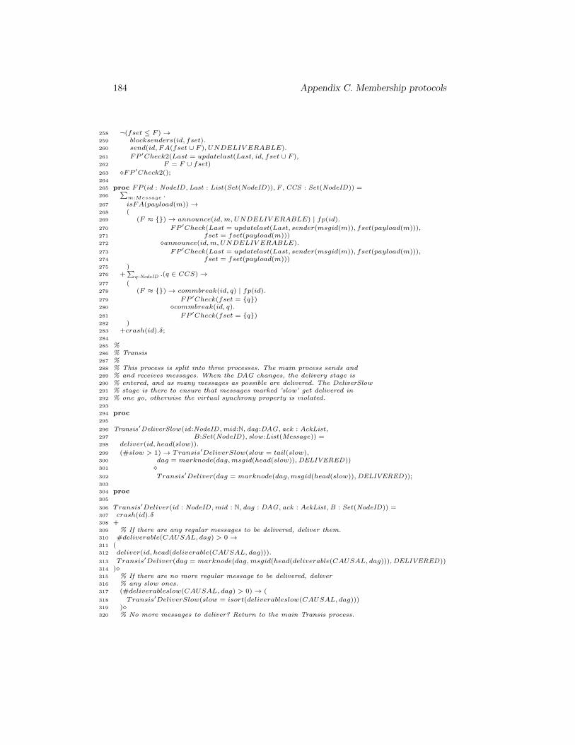
184 Appendix C. Membership protocols
258 ¬(fset ≤ F )→259 blocksenders(id, fset).260 send(id, FA(fset ∪ F ), UNDELIV ERABLE).
261 FP ′Check2(Last = updatelast(Last, id, fset ∪ F ),262 F = F ∪ fset)263 �FP ′Check2();264
265 proc FP (id : NodeID,Last : List(Set(NodeID)),F ,CCS : Set(NodeID)) =266
∑m:Message .
267 isFA(payload(m))→268 (269 (F ≈ {})→ announce(id,m,UNDELIV ERABLE) | fp(id).
270 FP ′Check(Last = updatelast(Last, sender(msgid(m)), fset(payload(m))),271 fset = fset(payload(m)))272 �announce(id,m,UNDELIV ERABLE).
273 FP ′Check(Last = updatelast(Last, sender(msgid(m)), fset(payload(m))),274 fset = fset(payload(m)))275 )276 +
∑q:NodeID .(q ∈ CCS)→
277 (278 (F ≈ {})→ commbreak(id, q) | fp(id).
279 FP ′Check(fset = {q})280 �commbreak(id, q).
281 FP ′Check(fset = {q})282 )283 +crash(id).δ;284
285 %286 % Transis287 %288 % This process is split into three processes. The main process sends and289 % and receives messages. When the DAG changes, the delivery stage is290 % entered, and as many messages as possible are delivered. The DeliverSlow291 % stage is there to ensure that messages marked ’slow’ get delivered in292 % one go, otherwise the virtual synchrony property is violated.293
294 proc295
296 Transis′DeliverSlow(id:NodeID,mid:N, dag:DAG, ack : AckList,297 B:Set(NodeID), slow :List(Message)) =298 deliver(id, head(slow)).
299 (#slow > 1)→ Transis′DeliverSlow(slow = tail(slow),300 dag = marknode(dag,msgid(head(slow)),DELIVERED))301 �302 Transis′Deliver(dag = marknode(dag,msgid(head(slow)),DELIVERED));303
304 proc305
306 Transis′Deliver(id : NodeID,mid : N, dag : DAG, ack : AckList,B : Set(NodeID)) =307 crash(id).δ308 +309 % If there are any regular messages to be delivered, deliver them.310 #deliverable(CAUSAL, dag) > 0→311 (312 deliver(id, head(deliverable(CAUSAL, dag))).
313 Transis′Deliver(dag = marknode(dag,msgid(head(deliverable(CAUSAL, dag))),DELIVERED))314 )�315 % If there are no more regular message to be delivered, deliver316 % any slow ones.317 (#deliverableslow(CAUSAL, dag) > 0)→ (
318 Transis′DeliverSlow(slow = isort(deliverableslow(CAUSAL, dag)))319 )�320 % No more messages to deliver? Return to the main Transis process.
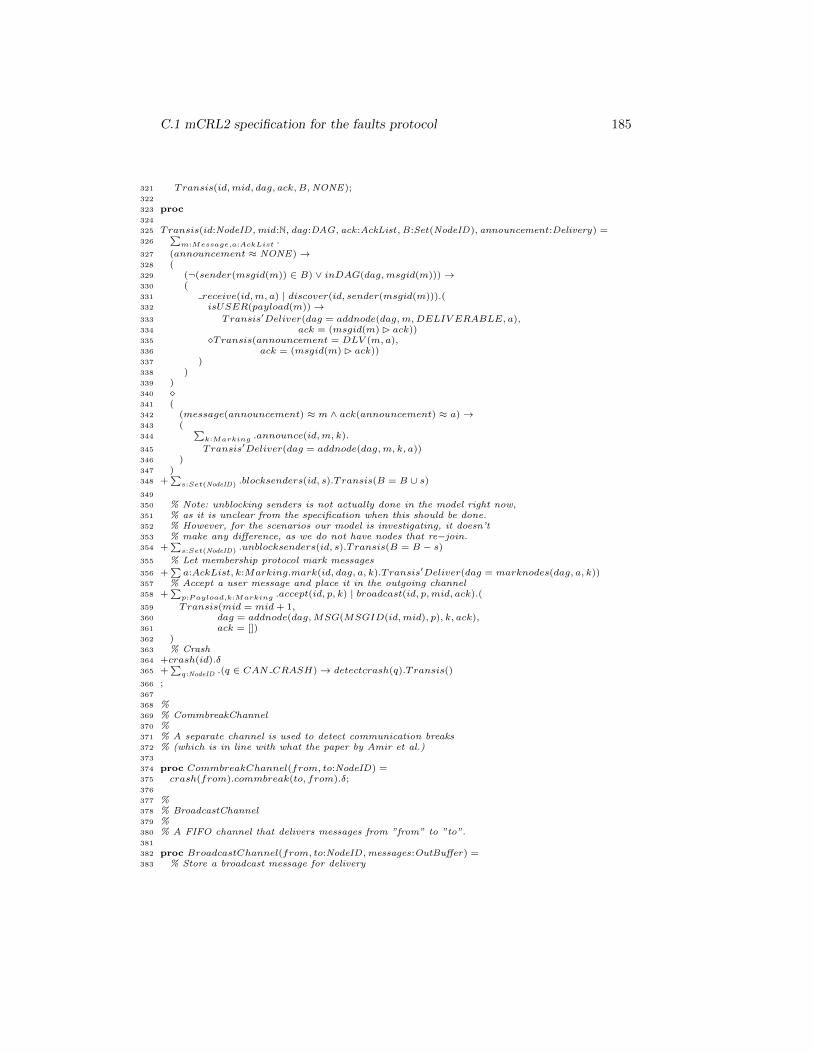
C.1 mCRL2 specification for the faults protocol 185
321 Transis(id,mid, dag, ack,B,NONE);322
323 proc324
325 Transis(id:NodeID,mid:N, dag:DAG, ack :AckList,B :Set(NodeID), announcement:Delivery) =326
∑m:Message,a:AckList .
327 (announcement ≈ NONE)→328 (329 (¬(sender(msgid(m)) ∈ B) ∨ inDAG(dag,msgid(m)))→330 (331 receive(id,m, a) | discover(id, sender(msgid(m))).(332 isUSER(payload(m))→333 Transis′Deliver(dag = addnode(dag,m,DELIV ERABLE, a),334 ack = (msgid(m) � ack))335 �Transis(announcement = DLV (m, a),336 ack = (msgid(m) � ack))337 )338 )339 )340 �341 (342 (message(announcement) ≈ m ∧ ack(announcement) ≈ a)→343 (344
∑k:Marking .announce(id,m, k).
345 Transis′Deliver(dag = addnode(dag,m, k, a))346 )347 )348 +
∑s:Set(NodeID) .blocksenders(id, s).Transis(B = B ∪ s)
349
350 % Note: unblocking senders is not actually done in the model right now,351 % as it is unclear from the specification when this should be done.352 % However, for the scenarios our model is investigating, it doesn’t353 % make any difference, as we do not have nodes that re−join.354 +
∑s:Set(NodeID) .unblocksenders(id, s).Transis(B = B − s)
355 % Let membership protocol mark messages
356 +∑a:AckList, k:Marking.mark(id, dag, a, k).Transis′Deliver(dag = marknodes(dag, a, k))
357 % Accept a user message and place it in the outgoing channel358 +
∑p:Payload,k:Marking .accept(id, p, k) | broadcast(id, p,mid, ack).(
359 Transis(mid = mid+ 1,360 dag = addnode(dag,MSG(MSGID(id,mid), p), k, ack),361 ack = [])362 )363 % Crash364 +crash(id).δ365 +
∑q:NodeID .(q ∈ CAN CRASH)→ detectcrash(q).Transis()
366 ;367
368 %369 % CommbreakChannel370 %371 % A separate channel is used to detect communication breaks372 % (which is in line with what the paper by Amir et al.)373
374 proc CommbreakChannel(from, to:NodeID) =375 crash(from).commbreak(to, from).δ;376
377 %378 % BroadcastChannel379 %380 % A FIFO channel that delivers messages from ”from” to ”to”.381
382 proc BroadcastChannel(from, to:NodeID,messages:OutBuffer) =383 % Store a broadcast message for delivery
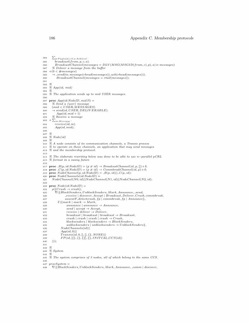
186 Appendix C. Membership protocols
384∑
p:Payload,c:N,a:AckList .
385 broadcast(from, p, c, a).386 BroadcastChannel(messages = DLV (MSG(MSGID(from, c), p), a) �messages)387 % Deliver a message from the buffer388 +(0 < #messages)389 → send(to,message(rhead(messages)), ack(rhead(messages))).390 BroadcastChannel(messages = rtail(messages));391
392 %393 % App(id, mid)394 %395 % The application sends up to mid USER messages.396
397 proc App(id:NodeID,mid:N) =398 % Send a (user) message399 (mid < USER MESSAGES)400 → send(id, USER,DELIV ERABLE).401 App(id,mid+ 1)402 % Receive a message403 +
∑m:Message .
404 receive(id,m).405 App(id,mid);406
407 %408 % Node(id)409 %410 % A node consists of its communication channels, a Transis process411 % to operate on those channels, an application that may send messages412 % and the membership protocol.413
414 % The elaborate rewriting below was done to be able to use n−parallel pCRL415 % format in a sunny future416
417 proc B(p, id:NodeID) = (p 6= id)→ BroadcastChannel(id, p, []) � δ;418 proc C(p, id:NodeID) = (p 6= id)→ CommbreakChannel(id, p) � δ;419 proc NodeChannel(p, id:NodeID) = B(p, id)|| C (p, id);420 proc NodeChannels(id:NodeID) =421 NodeChannel(N0, id)||NodeChannel(N1, id)||NodeChannel(N2, id);422
423 proc Node(id:NodeID) =424 ρ({Crash→ crash},425 ∇({BlockSenders, UnblockSenders,Mark,Announce, send,426 receive | discover, Accept | Broadcast,Deliver, Crash, commbreak,427 assentF, detectcrash, fp | commbreak, fp | Announce},428 Γ({mark | mark →Mark,429 announce | announce→ Announce,430 send | accept→ Accept,431 receive | deliver → Deliver,432 broadcast | broadcast | broadcast→ Broadcast,433 crash | crash | crash | crash→ Crash,434 blocksenders | blocksenders→ BlockSenders,435 unblocksenders | unblocksenders→ UnblockSenders},436 NodeChannels(id)||437 App(id, 0)||438 Transis(id, 0, [], [], {},NONE)||439 FP (id, [{}, {}, {}], {}, INITIAL CCS(id))440 )));441
442 %443 % System444 %445 % The system comprises of 3 nodes, all of which belong to the same CCS.446
447 procSystem =448 ∇({BlockSenders, UnblockSenders,Mark,Announce, comm | discover,
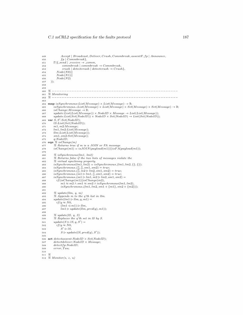
C.1 mCRL2 specification for the faults protocol 187
449 Accept | Broadcast,Deliver, Crash, Commbreak, assentF, fp | Announce,450 fp | Commbreak},451 Γ({ send | receive→ comm,452 commbreak | commbreak → Commbreak,453 crash | detectcrash | detectcrash→ Crash},454 Node(N0)||455 Node(N1)||456 Node(N2)457 ));458
459
460 % −−−−−−−−−−−−−−−−−−−−−−−−−−−−−−−−−−−−−−−−−−−−−−−−−−−461 % Monitoring462 % −−−−−−−−−−−−−−−−−−−−−−−−−−−−−−−−−−−−−−−−−−−−−−−−−−−463
464 map isSynchronous:List(Message)× List(Message)→ B;465 isSynchronous :List(Message)× List(Message)× Set(Message)× Set(Message)→ B;466 isChange:Message→ B;467 update:List(List(Message))× NodeID ×Message → List(List(Message));468 update:List(Set(NodeID))× NodeID × Set(NodeID)→ List(Set(NodeID));
469 var S, S′:Set(NodeID);470 lS:List(Set(NodeID));471 m1,m2:Message;472 lm1, lm2:List(Message);473 llm:List(List(Message));474 sm1, sm2:Set(Message);475 q:NodeID;476 eqn % isChange(m)477 % Returns true if m is a JOIN or FA message478 isChange(m1) = isJOIN(payload(m1))||isFA(payload(m1));479
480 % isSynchronous(lm1, lm2)481 % Returns false if the two lists of messages violate the482 % virtual synchrony property.483 isSynchronous(lm1, lm2) = isSynchronous (lm1, lm2, {}, {});484 isSynchronous ([], [], sm1, sm2) = true;485 isSynchronous ([],m2 � lm2, sm1, sm2) = true;486 isSynchronous (m1 � lm1, [], sm1, sm2) = true;487 isSynchronous (m1 � lm1,m2 � lm2, sm1, sm2) =488 if(isChange(m1)||isChange(m2),489 m1 ≈ m2 ∧ sm1 ≈ sm2 ∧ isSynchronous(lm1, lm2),490 isSynchronous (lm1, lm2, sm1 + {m1}, sm2 + {m2}));491
492 % update(llm, q, m)493 % Appends m to the q’th list in llm.494 update(lm1 � llm, q,m1) =495 if(q ≈ N0,496 (lm1 �m1) � llm,497 lm1 � update(llm, pred(q),m1));498
499 % update(lS, q, S)500 % Replaces the q’th set in lS by S.
501 update(S � lS, q, S′) =502 if(q ≈ N0,
503 S′ � lS,
504 S � update(lS, pred(q), S′));505
506 act detectassent:NodeID × Set(NodeID);507 detectdeliver:NodeID ×Message;508 detectfp:NodeID;509 error, Tau;510
511 %512 % Monitor(s, c, u)
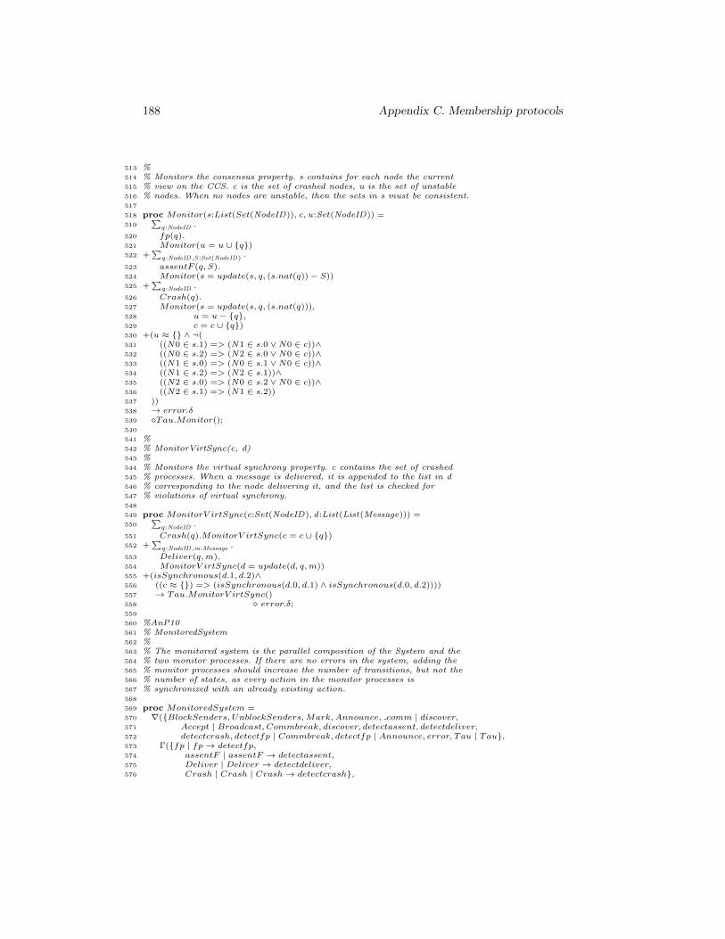
188 Appendix C. Membership protocols
513 %514 % Monitors the consensus property. s contains for each node the current515 % view on the CCS. c is the set of crashed nodes, u is the set of unstable516 % nodes. When no nodes are unstable, then the sets in s must be consistent.517
518 proc Monitor(s:List(Set(NodeID)), c, u:Set(NodeID)) =519
∑q:NodeID .
520 fp(q).521 Monitor(u = u ∪ {q})522 +
∑q:NodeID,S:Set(NodeID) .
523 assentF (q, S).524 Monitor(s = update(s, q, (s.nat(q))− S))525 +
∑q:NodeID .
526 Crash(q).527 Monitor(s = update(s, q, (s.nat(q))),528 u = u− {q},529 c = c ∪ {q})530 +(u ≈ {} ∧ ¬(531 ((N0 ∈ s.1) => (N1 ∈ s.0 ∨N0 ∈ c))∧532 ((N0 ∈ s.2) => (N2 ∈ s.0 ∨N0 ∈ c))∧533 ((N1 ∈ s.0) => (N0 ∈ s.1 ∨N0 ∈ c))∧534 ((N1 ∈ s.2) => (N2 ∈ s.1))∧535 ((N2 ∈ s.0) => (N0 ∈ s.2 ∨N0 ∈ c))∧536 ((N2 ∈ s.1) => (N1 ∈ s.2))537 ))538 → error.δ539 �Tau.Monitor();540
541 %542 % MonitorVirtSync(c, d)543 %544 % Monitors the virtual synchrony property. c contains the set of crashed545 % processes. When a message is delivered, it is appended to the list in d546 % corresponding to the node delivering it, and the list is checked for547 % violations of virtual synchrony.548
549 proc MonitorV irtSync(c:Set(NodeID), d:List(List(Message))) =550
∑q:NodeID .
551 Crash(q).MonitorV irtSync(c = c ∪ {q})552 +
∑q:NodeID,m:Message .
553 Deliver(q,m).554 MonitorV irtSync(d = update(d, q,m))555 +(isSynchronous(d.1, d.2)∧556 ((c ≈ {}) => (isSynchronous(d.0, d.1) ∧ isSynchronous(d.0, d.2))))557 → Tau.MonitorV irtSync()558 � error.δ;559
560 %AnP10561 % MonitoredSystem562 %563 % The monitored system is the parallel composition of the System and the564 % two monitor processes. If there are no errors in the system, adding the565 % monitor processes should increase the number of transitions, but not the566 % number of states, as every action in the monitor processes is567 % synchronized with an already existing action.568
569 proc MonitoredSystem =570 ∇({BlockSenders, UnblockSenders,Mark,Announce, comm | discover,571 Accept | Broadcast, Commbreak, discover, detectassent, detectdeliver,572 detectcrash, detectfp | Commbreak, detectfp | Announce, error, Tau | Tau},573 Γ({fp | fp→ detectfp,574 assentF | assentF → detectassent,575 Deliver | Deliver → detectdeliver,576 Crash | Crash | Crash→ detectcrash},
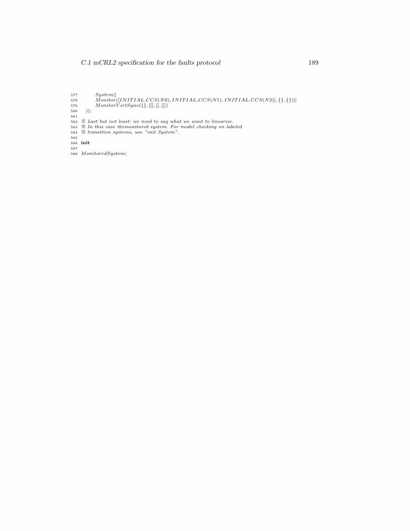
C.1 mCRL2 specification for the faults protocol 189
577 System||578 Monitor([INITIAL CCS(N0), INITIAL CCS(N1), INITIAL CCS(N2)], {}, {})||579 MonitorV irtSync({}, [[], [], []])580 ));581
582 % Last but not least: we need to say what we want to linearize.583 % In this case themonitored system. For model checking on labeled584 % transition systems, use ”init System”.585
586 init587
588 MonitoredSystem;
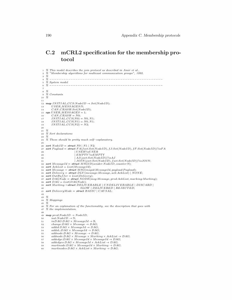
190 Appendix C. Membership protocols
C.2 mCRL2 specification for the membership pro-tocol
1 % This model describes the join protocol as described in Amir et al.,2 % ”Membership algorithms for multicast communication groups”, 1992.3 %4 % −−−−−−−−−−−−−−−−−−−−−−−−−−−−−−−−−−−−−−−−−−−−−−−−5 % System model6 % −−−−−−−−−−−−−−−−−−−−−−−−−−−−−−−−−−−−−−−−−−−−−−−−7
8 %9 % Constants
10 %11
12 map INITIAL CCS:NodeID → Set(NodeID);13 USER MESSAGES:N;14 CAN CRASH:Set(NodeID);15 eqn USER MESSAGES = 1;16 CAN CRASH = N0;17 INITIAL CCS(N0) = N0, N1;18 INITIAL CCS(N1) = N0, N1;19 INITIAL CCS(N2) = N2;20
21 %22 % Sort declarations23 %24 % These should be pretty much self−explanatory.25
26 sort NodeID = struct N0 | N1 | N2;27 sort Payload = struct FA(fset:Set(NodeID), fJ:Set(NodeID), fF :Set(NodeID))?isFA28 | USER?isUSER29 | EMPTY ?isEMPTY30 | AJ(jset:Set(NodeID))?isAJ31 | JOIN(jset:Set(NodeID), fset:Set(NodeID))?isJOIN ;32 sort MessageId = struct MSGID(sender:NodeID, counter:N);33 sort AckList = List(MessageId);34 sort Message = struct MSG(msgid:MessageId, payload:Payload);35 sort Delivery = struct DLV (message:Message, ack:AckList) | NONE;36 sort OutBuffer = List(Delivery);37 sort DAGNode = struct NODE(msg:Message, pred:AckList,marking:Marking);38 sort DAG = List(DAGNode);39 sort Marking =struct DELIV ERABLE | UNDELIV ERABLE | DISCARD |40 SLOW | DELIV ERED | REJECTED;41 sort DeliveryMode = struct BASIC | CAUSAL;42
43 %44 % Mappings45 %46 % For an explanation of the functionality, see the description that goes with47 % the implementation.48
49 map pred:NodeID → NodeID;50 nat:NodeID → N;51 inDAG:DAG×MessageId→ B;52 change:DAG×Message→ DAG;53 addid:DAG×MessageId→ DAG;54 addid :DAG×MessageId→ DAG;55 addnode:DAG×Message→ DAG;56 addnode:DAG×Message×Marking × AckList→ DAG;57 addedge:DAG×MessageId×MessageId→ DAG;58 addedges:DAG×MessageId× AckList→ DAG;59 marknode:DAG×MessageId×Marking → DAG;60 marknodes:DAG× AckList×Marking → DAG;
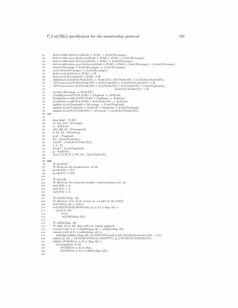
C.2 mCRL2 specification for the membership protocol 191
61 deliverable:DeliveryMode×DAG→ List(Message);62 deliverable aux:DeliveryMode×DAG×DAG→ List(Message);63 deliverableslow:DeliveryMode×DAG→ List(Message);64 deliverableslow aux:DeliveryMode×DAG×DAG× List(Message)→ List(Message);65 insert:Message× List(Message)→ List(Message);66 isort:List(Message)→ List(Message);67 delivered:AckList×DAG→ B;68 delivered:MessageId×DAG→ B;69 addtolast:List(Set(NodeID))×NodeID × Set(NodeID)→ List(Set(NodeID));70 JPConsensusF :Set(NodeID)× Set(NodeID)× List(Set(NodeID))→ B;71 JPConsensusJ:Set(NodeID)× Set(NodeID)× Set(NodeID)× List(Payload)×72 List(Set(NodeID))→ B;73 sender:Message→ NodeID;74 findRejectedJOIN :DAG× Payload→ AckList;75 findDeliverableJOIN :DAG× Payload→ AckList;76 findDeliverableFA:DAG× Set(NodeID)→ AckList;77 update:List(Payload)×Message→ List(Payload);78 update:List(Payload)×NodeID × Payload→ List(Payload);79 update:List(Set(NodeID))×Message→ List(Set(NodeID));80 var81
82 dag, dag1 : DAG;83 m,m1,m2 : Message;84 a : AckList;85 id1, id2, id : MessageId;86 k, k1, k2 : Marking;
87 p, p′ : Payload;88 lm : List(Message);89 LastF : List(Set(NodeID));90 r, n : N;91 LastJ : List(Payload);92 q : NodeID;93 fset, CCS, F, J, Fb, Fa : Set(NodeID);94
95 eqn96 % pred(id)97 % Returns the predecessor of id.98 pred(N2) = N1;99 pred(N1) = N0;
100
101 % nat(id)102 % Returns the natural number representation for id.103 nat(N0) = 0;104 nat(N1) = 1;105 nat(N2) = 2;106
107 % inDAG(dag, id)108 % Returns true if id occurs as a node in the DAG.109 inDAG([], id) = false;110 inDAG(NODE(MSG(id1, p), a, k) � dag, id) =111 if(id ≈ id1,112 true,113 inDAG(dag, id));114
115 % addid(dag, id)116 % adds id to the dag with an empty payload117 counter(id) ≈ 0→ addid(dag, id) = addid (dag, id);118 counter(id) 6= 0→ addid(dag, id) =119 addedge(addid (dag, id), id,MSGID(sender(id), Int2Nat(counter(id)− 1)));120 addid ([], id) = [NODE(MSG(id, EMPTY ), [], UNDELIV ERABLE)];121 addid (NODE(m, a, k) � dag, id) =122 if(msgid(m) ≈ id,123 NODE(m, a, k) � dag,124 NODE(m, a, k) � addid (dag, id));125
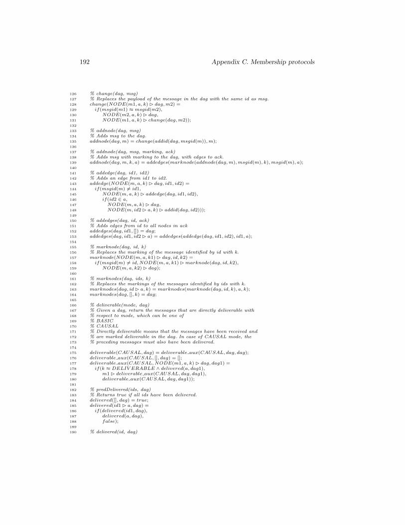
192 Appendix C. Membership protocols
126 % change(dag, msg)127 % Replaces the payload of the message in the dag with the same id as msg.128 change(NODE(m1, a, k) � dag,m2) =129 if(msgid(m1) ≈ msgid(m2),130 NODE(m2, a, k) � dag,131 NODE(m1, a, k) � change(dag,m2));132
133 % addnode(dag, msg)134 % Adds msg to the dag.135 addnode(dag,m) = change(addid(dag,msgid(m)),m);136
137 % addnode(dag, msg, marking, ack)138 % Adds msg with marking to the dag, with edges to ack.139 addnode(dag,m, k, a) = addedges(marknode(addnode(dag,m),msgid(m), k),msgid(m), a);140
141 % addedge(dag, id1, id2)142 % Adds an edge from id1 to id2.143 addedge(NODE(m, a, k) � dag, id1, id2) =144 if(msgid(m) 6= id1,145 NODE(m, a, k) � addedge(dag, id1, id2),146 if(id2 ∈ a,147 NODE(m, a, k) � dag,148 NODE(m, id2 � a, k) � addid(dag, id2)));149
150 % addedges(dag, id, ack)151 % Adds edges from id to all nodes in ack152 addedges(dag, id1, []) = dag;153 addedges(dag, id1, id2 � a) = addedges(addedge(dag, id1, id2), id1, a);154
155 % marknode(dag, id, k)156 % Replaces the marking of the message identified by id with k.157 marknode(NODE(m, a, k1) � dag, id, k2) =158 if(msgid(m) 6= id,NODE(m, a, k1) �marknode(dag, id, k2),159 NODE(m, a, k2) � dag);160
161 % marknodes(dag, ids, k)162 % Replaces the markings of the messages identified by ids with k.163 marknodes(dag, id� a, k) = marknodes(marknode(dag, id, k), a, k);164 marknodes(dag, [], k) = dag;165
166 % deliverable(mode, dag)167 % Given a dag, return the messages that are directly deliverable with168 % respect to mode, which can be one of169 % BASIC170 % CAUSAL171 % Directly deliverable means that the messages have been received and172 % are marked deliverable in the dag. In case of CAUSAL mode, the173 % preceding messages must also have been delivered.174
175 deliverable(CAUSAL, dag) = deliverable aux(CAUSAL, dag, dag);176 deliverable aux(CAUSAL, [], dag) = [];177 deliverable aux(CAUSAL,NODE(m1, a, k) � dag, dag1) =178 if(k ≈ DELIV ERABLE ∧ delivered(a, dag1),179 m1 � deliverable aux(CAUSAL, dag, dag1),180 deliverable aux(CAUSAL, dag, dag1));181
182 % predDelivered(ids, dag)183 % Returns true if all ids have been delivered.184 delivered([], dag) = true;185 delivered(id1 � a, dag) =186 if(delivered(id1, dag),187 delivered(a, dag),188 false);189
190 % delivered(id, dag)
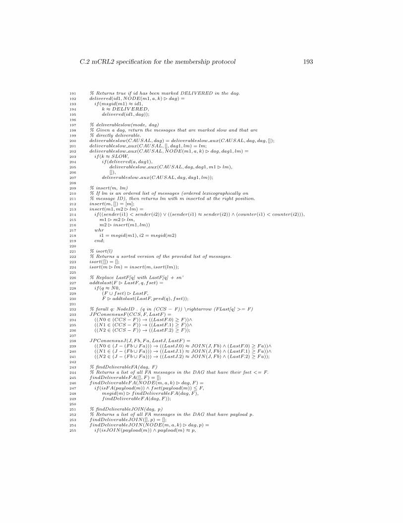
C.2 mCRL2 specification for the membership protocol 193
191 % Returns true if id has been marked DELIVERED in the dag.192 delivered(id1, NODE(m1, a, k) � dag) =193 if(msgid(m1) ≈ id1,194 k ≈ DELIV ERED,195 delivered(id1, dag));196
197 % deliverableslow(mode, dag)198 % Given a dag, return the messages that are marked slow and that are199 % directly deliverable.200 deliverableslow(CAUSAL, dag) = deliverableslow aux(CAUSAL, dag, dag, []);201 deliverableslow aux(CAUSAL, [], dag1, lm) = lm;202 deliverableslow aux(CAUSAL,NODE(m1, a, k) � dag, dag1, lm) =203 if(k ≈ SLOW,204 if(delivered(a, dag1),205 deliverableslow aux(CAUSAL, dag, dag1,m1 � lm),206 []),207 deliverableslow aux(CAUSAL, dag, dag1, lm));208
209 % insert(m, lm)210 % If lm is an ordered list of messages (ordered lexicographically on211 % message ID), then returns lm with m inserted at the right position.212 insert(m, []) = [m];213 insert(m1,m2 � lm) =214 if((sender(i1) < sender(i2)) ∨ ((sender(i1) ≈ sender(i2)) ∧ (counter(i1) < counter(i2))),215 m1 �m2 � lm,216 m2 � insert(m1, lm))217 whr218 i1 = msgid(m1), i2 = msgid(m2)219 end;220
221 % isort(l)222 % Returns a sorted version of the provided list of messages.223 isort([]) = [];224 isort(m� lm) = insert(m, isort(lm));225
226 % Replace LastF[q] with LastF[q] + sn’227 addtolast(F � LastF, q, fset) =228 if(q ≈ N0,229 (F ∪ fset) � LastF,230 F � addtolast(LastF, pred(q), fset));231
232 % forall q: NodeID . (q in (CCS − F)) \rightarrow (FLast[q] >= F)233 JPConsensusF (CCS, F, LastF ) =234 ((N0 ∈ (CCS − F ))→ ((LastF.0) ≥ F ))∧235 ((N1 ∈ (CCS − F ))→ ((LastF.1) ≥ F ))∧236 ((N2 ∈ (CCS − F ))→ ((LastF.2) ≥ F ));237
238 JPConsensusJ(J, Fb, Fa, LastJ, LastF ) =239 ((N0 ∈ (J − (Fb ∪ Fa)))→ ((LastJ.0) ≈ JOIN(J, Fb) ∧ (LastF.0) ≥ Fa))∧240 ((N1 ∈ (J − (Fb ∪ Fa)))→ ((LastJ.1) ≈ JOIN(J, Fb) ∧ (LastF.1) ≥ Fa))∧241 ((N2 ∈ (J − (Fb ∪ Fa)))→ ((LastJ.2) ≈ JOIN(J, Fb) ∧ (LastF.2) ≥ Fa));242
243 % findDeliverableFA(dag, F)244 % Returns a list of all FA messages in the DAG that have their fset <= F.245 findDeliverableFA([], F ) = [];246 findDeliverableFA(NODE(m, a, k) � dag, F ) =247 if(isFA(payload(m)) ∧ fset(payload(m)) ≤ F,248 msgid(m) � findDeliverableFA(dag, F ),249 findDeliverableFA(dag, F ));250
251 % findDeliverableJOIN(dag, p)252 % Returns a list of all FA messages in the DAG that have payload p.253 findDeliverableJOIN([], p) = [];254 findDeliverableJOIN(NODE(m, a, k) � dag, p) =255 if(isJOIN(payload(m)) ∧ payload(m) ≈ p,
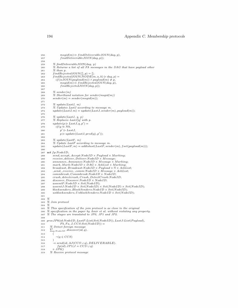
194 Appendix C. Membership protocols
256 msgid(m) � findDeliverableJOIN(dag, p),257 findDeliverableJOIN(dag, p));258
259 % findDeliverableJOIN(dag, p)260 % Returns a list of all FA messages in the DAG that have payload other261 % than p.262 findRejectedJOIN([], p) = [];263 findRejectedJOIN(NODE(m, a, k) � dag, p) =264 if(isJOIN(payload(m)) ∧ payload(m) 6= p,265 msgid(m) � findRejectedJOIN(dag, p),266 findRejectedJOIN(dag, p));267
268 % sender(m)269 % Shorthand notation for sender(msgid(m))270 sender(m) = sender(msgid(m));271
272 % update(LastJ, m)273 % Updates LastJ according to message m.274 update(LastJ,m) = update(LastJ, sender(m), payload(m));275
276 % update(LastJ, q, p)277 % Replaces LastJ[q] with p.
278 update(p� LastJ, q, p′) =279 if(q ≈ N0,
280 p′ � LastJ,
281 p� update(LastJ, pred(q), p′));282
283 % update(LastF, m)284 % Update LastF according to message m.285 update(LastF,m) = addtolast(LastF, sender(m), fset(payload(m)));286
287 act fp:NodeID;288 send, accept, Accept:NodeID × Payload×Marking;289 receive, deliver,Deliver:NodeID ×Message;290 announce,Announce:NodeID ×Message×Marking;291 mark,Mark:NodeID ×DAG× AckList×Marking;292 broadcast, Broadcast:NodeID × Payload× N× AckList;293 send, receive, comm:NodeID ×Message× AckList;294 commbreak, Commbreak:NodeID ×NodeID;295 crash, detectcrash, Crash,DetectCrash:NodeID;296 discover,Discover:NodeID ×NodeID;297 assentF :NodeID × Set(NodeID);298 assentJ:NodeID × Set(NodeID)× Set(NodeID)× Set(NodeID);299 blocksenders,BlockSenders:NodeID × Set(NodeID);300 unblocksenders, UnblockSenders:NodeID × Set(NodeID);301
302 %303 % Join protocol304 %305 % This specification of the join protocol is as close to the original306 % specification in the paper by Amir et al. without violating any property.307 % The stages are translated to JP0, JP1 and JP2.308
309 procJP0(id:NodeID,LastF :List(Set(NodeID)), LastJ:List(Payload),310 Fb, Fa, J, CCS:Set(NodeID)) =311 % Detect foreign message312
∑q:NodeID .discover(id, q).
313 (314 ¬(q ∈ CCS)315 )316 → send(id, AJ(CCS ∪ q), DELIV ERABLE).317 fp(id).JP1(J = CCS ∪ q)318 � JP0()319 % Receive protocol message
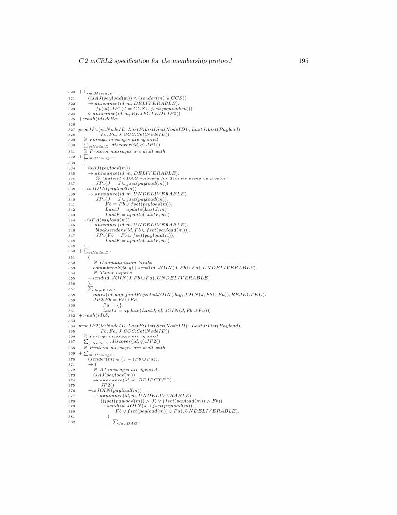
C.2 mCRL2 specification for the membership protocol 195
320 +∑
m:Message .
321 (isAJ(payload(m)) ∧ (sender(m) ∈ CCS))322 → announce(id,m,DELIV ERABLE).323 fp(id).JP1(J = CCS ∪ jset(payload(m)))324 � announce(id,m,REJECTED).JP0()325 +crash(id).delta;326
327 procJP1(id:NodeID,LastF :List(Set(NodeID)), LastJ:List(Payload),328 Fb, Fa, J, CCS:Set(NodeID)) =329 % Foreign messages are ignored330
∑q:NodeID .discover(id, q).JP1()
331 % Protocol messages are dealt with332 +
∑m:Message .
333 (334 isAJ(payload(m))335 → announce(id,m,DELIV ERABLE).336 % ”Extend CDAG recovery for Transis using cut vector”337 JP1(J = J ∪ jset(payload(m)))338 +isJOIN(payload(m))339 → announce(id,m,UNDELIV ERABLE).340 JP1(J = J ∪ jset(payload(m)),341 Fb = Fb ∪ fset(payload(m)),342 LastJ = update(LastJ,m),343 LastF = update(LastF,m))344 +isFA(payload(m))345 → announce(id,m,UNDELIV ERABLE).346 blocksenders(id, Fb ∪ fset(payload(m))).347 JP1(Fb = Fb ∪ fset(payload(m)),348 LastF = update(LastF,m))349 )350 +
∑q:NodeID .
351 (352 % Communication breaks353 commbreak(id, q) | send(id, JOIN(J, Fb ∪ Fa), UNDELIV ERABLE)354 % Timer expires355 +send(id, JOIN(J, Fb ∪ Fa), UNDELIV ERABLE)356 ).357
∑dag:DAG .
358 mark(id, dag, findRejectedJOIN(dag, JOIN(J, Fb ∪ Fa)), REJECTED).359 JP2(Fb = Fb ∪ Fa,360 Fa = {},361 LastJ = update(LastJ, id, JOIN(J, Fb ∪ Fa)))362 +crash(id).δ;363
364 procJP2(id:NodeID,LastF :List(Set(NodeID)), LastJ:List(Payload),365 Fb, Fa, J, CCS:Set(NodeID)) =366 % Foreign messages are ignored367
∑q:NodeID .discover(id, q).JP2()
368 % Protocol messages are dealt with369 +
∑m:Message .
370 (sender(m) ∈ (J − (Fb ∪ Fa)))371 → (372 % AJ messages are ignored373 isAJ(payload(m))374 → announce(id,m,REJECTED).375 JP2()376 +isJOIN(payload(m))377 → announce(id,m,UNDELIV ERABLE).378 ((jset(payload(m)) > J) ∨ (fset(payload(m)) > Fb))379 → send(id, JOIN(J ∪ jset(payload(m)),380 Fb ∪ fset(payload(m)) ∪ Fa), UNDELIV ERABLE).381 (382
∑dag:DAG .
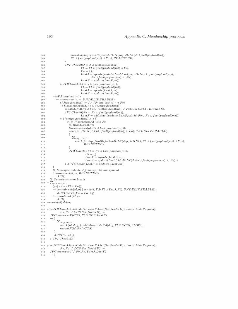
196 Appendix C. Membership protocols
383 mark(id, dag, findRejectedJOIN(dag, JOIN(J ∪ jset(payload(m)),384 Fb ∪ fset(payload(m)) ∪ Fa)), REJECTED)385 ).
386 JP2′Check0(J = J ∪ jset(payload(m)),387 Fb = Fb ∪ fset(payload(m)) ∪ Fa,388 Fa = {},389 LastJ = update(update(LastJ,m), id, JOIN(J ∪ jset(payload(m)),390 Fb ∪ fset(payload(m)) ∪ Fa)),391 LastF = update(LastF,m))
392 � JP2′Check0(J = J ∪ jset(payload(m)),393 Fb = Fb ∪ fset(payload(m)),394 LastJ = update(LastJ,m),395 LastF = update(LastF,m))396 +isFA(payload(m))397 → announce(id,m,UNDELIV ERABLE).398 (fJ(payload(m)) ≈ J ∧ fF (payload(m)) ≈ Fb)399 → blocksenders(id, Fa ∪ fset(payload(m))).400 send(id, FA(Fb ∪ Fa ∪ fset(payload(m)), J, Fb), UNDELIV ERABLE).
401 JP2′Check0(Fa = Fa ∪ fset(payload(m)),402 LastF = addtolast(update(LastF,m), id, Fb ∪ Fa ∪ fset(payload(m))))403 � (fset(payload(m)) > Fb)404 −> % IncorporateFA into Fb405 % BroadcastJOIN406 blocksenders(id, Fb ∪ fset(payload(m))).407 send(id, JOIN(J, Fb ∪ fset(payload(m)) ∪ Fa), UNDELIV ERABLE).408 (409
∑dag:DAG .
410 mark(id, dag, findRejectedJOIN(dag, JOIN(J, Fb ∪ fset(payload(m)) ∪ Fa)),411 REJECTED)412 ).
413 JP2′Check0(Fb = Fb ∪ fset(payload(m)),414 Fa = {},415 LastF = update(LastF,m),416 LastJ = update(LastJ, id, JOIN(J, Fb ∪ fset(payload(m)) ∪ Fa)))
417 � JP2′Check0(LastF = update(LastF,m))418 )419 % Messages outside J\(Fb\cup Fa) are ignored420 � announce(id,m,REJECTED).421 JP2()422 % Communication breaks423 +
∑q:NodeID .
424 (q ∈ (J − (Fb ∪ Fa)))425 → commbreak(id, q) | send(id, FA(Fb ∪ Fa, J, Fb), UNDELIV ERABLE).
426 JP2′Check0(Fa = Fa ∪ q)427 � commbreak(id, q).428 JP2()429 +crash(id).delta;430
431 procJP2′Check0(id:NodeID,LastF :List(Set(NodeID)), LastJ:List(Payload),432 Fb, Fa, J, CCS:Set(NodeID)) =433 JPConsensusF (CCS, Fb ∩ CCS,LastF )434 → (435
∑dag:DAG .
436 mark(id, dag, findDeliverableFA(dag, Fb ∩ CCS), SLOW ).437 assentF (id, Fb ∩ CCS)438 ).
439 JP2′Check1()
440 � JP2′Check1();441
442 procJP2′Check1(id:NodeID,LastF :List(Set(NodeID)), LastJ:List(Payload),443 Fb, Fa, J, CCS:Set(NodeID)) =444 JPConsensusJ(J, Fb, Fa, LastJ, LastF )445 → (
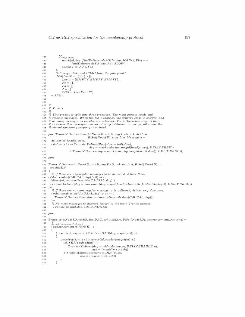
C.2 mCRL2 specification for the membership protocol 197
446∑
dag:DAG .
447 mark(id, dag, findDeliverableJOIN(dag, JOIN(J, Fb)) + +448 findDeliverableFA(dag, Fa), SLOW ).449 assentJ(id, J, Fb, Fa)450 ).451 % ”merge DAG and CDAG from the join point”452 JP0(LastF = [{}, {}, {}],453 LastJ = [EMPTY,EMPTY,EMPTY ],454 Fb = {},455 Fa = {},456 J = {},457 CCS = J − (Fa ∪ Fb))458 � JP2();459
460
461 %462 % Transis463 %464 % This process is split into three processes. The main process sends and465 % receives messages. When the DAG changes, the delivery stage is entered, and466 % as many messages as possible are delivered. The DeliverSlow stage is there467 % to ensure that messages marked ’slow’ get delivered in one go, otherwise the468 % virtual synchrony property is violated.469
470 proc Transis′DeliverSlow(id:NodeID,mid:N, dag:DAG, ack:AckList,471 B:Set(NodeID), slow:List(Message)) =472 deliver(id, head(slow)).
473 (#slow > 1)→ Transis′DeliverSlow(slow = tail(slow),474 dag = marknode(dag,msgid(head(slow)), DELIV ERED))
475 � Transis′Deliver(dag = marknode(dag,msgid(head(slow)), DELIV ERED));476
477 proc478
479 Transis′Deliver(id:NodeID,mid:N, dag:DAG, ack:AckList, B:Set(NodeID)) =480 crash(id).δ481 +482 % If there are any regular messages to be delivered, deliver them.483 (#deliverable(CAUSAL, dag) > 0)→ (484 deliver(id, head(deliverable(CAUSAL, dag))).
485 Transis′Deliver(dag = marknode(dag,msgid(head(deliverable(CAUSAL, dag))), DELIV ERED))486 ) �487 % If there are no more regular message to be delivered, deliver any slow ones.488 (#deliverableslow(CAUSAL, dag) > 0)→ (
489 Transis′DeliverSlow(slow = isort(deliverableslow(CAUSAL, dag)))490 ) �491 % No more messages to deliver? Return to the main Transis process.492 Transis(id,mid, dag, ack,B,NONE);493
494 proc495
496 Transis(id:NodeID,mid:N, dag:DAG, ack:AckList, B:Set(NodeID), announcement:Delivery) =497
∑m:Message,a:AckList .
498 (announcement ≈ NONE)→499 (500 (¬(sender(msgid(m)) ∈ B) ∨ inDAG(dag,msgid(m)))→501 (502 receive(id,m, a) | discover(id, sender(msgid(m))).(503 isUSER(payload(m))→504 Transis′Deliver(dag = addnode(dag,m,DELIV ERABLE, a),505 ack = (msgid(m) � ack))506 � Transis(announcement = DLV (m, a),507 ack = (msgid(m) � ack))508 )509 )
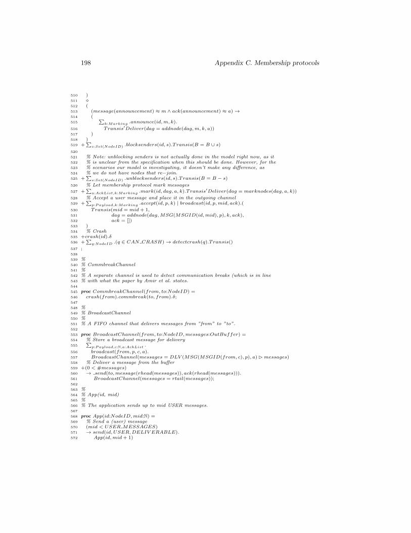
198 Appendix C. Membership protocols
510 )511 �512 (513 (message(announcement) ≈ m ∧ ack(announcement) ≈ a)→514 (515
∑k:Marking .announce(id,m, k).
516 Transis′Deliver(dag = addnode(dag,m, k, a))517 )518 )519 +
∑s:Set(NodeID) .blocksenders(id, s).Transis(B = B ∪ s)
520
521 % Note: unblocking senders is not actually done in the model right now, as it522 % is unclear from the specification when this should be done. However, for the523 % scenarios our model is investigating, it doesn’t make any difference, as524 % we do not have nodes that re−join.525 +
∑s:Set(NodeID) .unblocksenders(id, s).Transis(B = B − s)
526 % Let membership protocol mark messages
527 +∑
a:AckList,k:Marking .mark(id, dag, a, k).Transis′Deliver(dag = marknodes(dag, a, k))
528 % Accept a user message and place it in the outgoing channel529 +
∑p:Payload,k:Marking .accept(id, p, k) | broadcast(id, p,mid, ack).(
530 Transis(mid = mid+ 1,531 dag = addnode(dag,MSG(MSGID(id,mid), p), k, ack),532 ack = [])533 )534 % Crash535 +crash(id).δ536 +
∑q:NodeID .(q ∈ CAN CRASH)→ detectcrash(q).Transis()
537 ;538
539 %540 % CommbreakChannel541 %542 % A separate channel is used to detect communication breaks (which is in line543 % with what the paper by Amir et al. states.544
545 proc CommbreakChannel(from, to:NodeID) =546 crash(from).commbreak(to, from).δ;547
548 %549 % BroadcastChannel550 %551 % A FIFO channel that delivers messages from ”from” to ”to”.552
553 proc BroadcastChannel(from, to:NodeID,messages:OutBuffer) =554 % Store a broadcast message for delivery555
∑p:Payload,c:N,a:AckList .
556 broadcast(from, p, c, a).557 BroadcastChannel(messages = DLV (MSG(MSGID(from, c), p), a) �messages)558 % Deliver a message from the buffer559 +(0 < #messages)560 → send(to,message(rhead(messages)), ack(rhead(messages))).561 BroadcastChannel(messages = rtail(messages));562
563 %564 % App(id, mid)565 %566 % The application sends up to mid USER messages.567
568 proc App(id:NodeID,mid:N) =569 % Send a (user) message570 (mid < USER MESSAGES)571 → send(id, USER,DELIV ERABLE).572 App(id,mid+ 1)
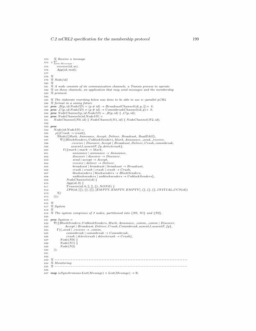
C.2 mCRL2 specification for the membership protocol 199
573 % Receive a message574 +
∑m:Message .
575 receive(id,m).576 App(id,mid);577
578 %579 % Node(id)580 %581 % A node consists of its communication channels, a Transis process to operate582 % on those channels, an application that may send messages and the membership583 % protocol.584
585 % The elaborate rewriting below was done to be able to use n−parallel pCRL586 % format in a sunny future587 proc B(p, id:NodeID) = (p 6= id)→ BroadcastChannel(id, p, []) � δ;588 proc C(p, id:NodeID) = (p 6= id)→ CommbreakChannel(id, p) � δ;589 proc NodeChannel(p, id:NodeID) = B(p, id) ‖ C(p, id);590 proc NodeChannels(id:NodeID) =591 NodeChannel(N0, id) ‖ NodeChannel(N1, id) ‖ NodeChannel(N2, id);592
593 proc594 Node(id:NodeID) =595 ρ({Crash→ crash},596 %hide({Mark, Announce, Accept, Deliver, Broadcast, ReadDAG},597 ∇({BlockSenders, UnblockSenders,Mark,Announce, send, receive,598 receive | Discover, Accept | Broadcast,Deliver, Crash, commbreak,599 assentJ, assentF, fp, detectcrash},600 Γ({mark | mark →Mark,601 announce | announce→ Announce,602 discover | discover → Discover,603 send | accept→ Accept,604 receive | deliver → Deliver,605 broadcast | broadcast | broadcast→ Broadcast,606 crash | crash | crash | crash→ Crash,607 blocksenders | blocksenders→ BlockSenders,608 unblocksenders | unblocksenders→ UnblockSenders},609 NodeChannels(id) ‖610 App(id, 0) ‖611 Transis(id, 0, [], [], {}, NONE) ‖612 JP0(id, [{}, {}, {}], [EMPTY,EMPTY,EMPTY ], {}, {}, {}, INITIAL CCS(id))613 %)614 )));615
616 %617 % System618 %619 % The system comprises of 3 nodes, partitioned into {N0, N1} and {N2}.620
621 proc System =622 ∇({BlockSenders, UnblockSenders,Mark,Announce, comm, comm | Discover,623 Accept | Broadcast,Deliver, Crash, Commbreak, assentJ, assentF, fp},624 Γ({ send | receive→ comm,625 commbreak | commbreak → Commbreak,626 crash | detectcrash | detectcrash→ Crash},627 Node(N0) ‖628 Node(N1) ‖629 Node(N2)630 ));631
632
633 % −−−−−−−−−−−−−−−−−−−−−−−−−−−−−−−−−−−−−−−−−−−−−−−−−−−634 % Monitoring635 % −−−−−−−−−−−−−−−−−−−−−−−−−−−−−−−−−−−−−−−−−−−−−−−−−−−636
637 map isSynchronous:List(Message)× List(Message)→ B;
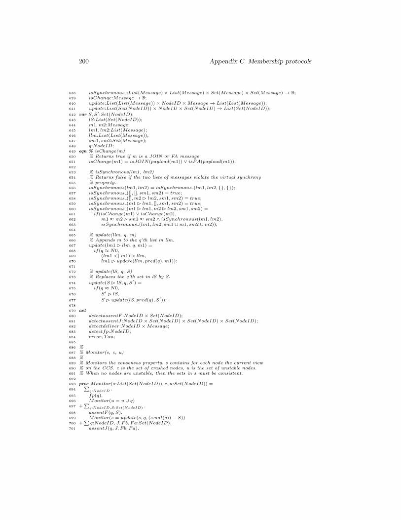
200 Appendix C. Membership protocols
638 isSynchronous :List(Message)× List(Message)× Set(Message)× Set(Message)→ B;639 isChange:Message→ B;640 update:List(List(Message))×NodeID ×Message→ List(List(Message));641 update:List(Set(NodeID))×NodeID × Set(NodeID)→ List(Set(NodeID));
642 var S, S′:Set(NodeID);643 lS:List(Set(NodeID));644 m1,m2:Message;645 lm1, lm2:List(Message);646 llm:List(List(Message));647 sm1, sm2:Set(Message);648 q:NodeID;649 eqn % isChange(m)650 % Returns true if m is a JOIN or FA message651 isChange(m1) = isJOIN(payload(m1)) ∨ isFA(payload(m1));652
653 % isSynchronous(lm1, lm2)654 % Returns false if the two lists of messages violate the virtual synchrony655 % property.656 isSynchronous(lm1, lm2) = isSynchronous (lm1, lm2, {}, {});657 isSynchronous ([], [], sm1, sm2) = true;658 isSynchronous ([],m2 � lm2, sm1, sm2) = true;659 isSynchronous (m1 � lm1, [], sm1, sm2) = true;660 isSynchronous (m1 � lm1,m2 � lm2, sm1, sm2) =661 if(isChange(m1) ∨ isChange(m2),662 m1 ≈ m2 ∧ sm1 ≈ sm2 ∧ isSynchronous(lm1, lm2),663 isSynchronous (lm1, lm2, sm1 ∪m1, sm2 ∪m2));664
665 % update(llm, q, m)666 % Appends m to the q’th list in llm.667 update(lm1 � llm, q,m1) =668 if(q ≈ N0,669 (lm1 <| m1) � llm,670 lm1 � update(llm, pred(q),m1));671
672 % update(lS, q, S)673 % Replaces the q’th set in lS by S.
674 update(S � lS, q, S′) =675 if(q ≈ N0,
676 S′ � lS,
677 S � update(lS, pred(q), S′));678
679 act680 detectassentF :NodeID × Set(NodeID);681 detectassentJ:NodeID × Set(NodeID)× Set(NodeID)× Set(NodeID);682 detectdeliver:NodeID ×Message;683 detectfp:NodeID;684 error, Tau;685
686 %687 % Monitor(s, c, u)688 %689 % Monitors the consensus property. s contains for each node the current view690 % on the CCS. c is the set of crashed nodes, u is the set of unstable nodes.691 % When no nodes are unstable, then the sets in s must be consistent.692
693 proc Monitor(s:List(Set(NodeID)), c, u:Set(NodeID)) =694
∑q:NodeID .
695 fp(q).696 Monitor(u = u ∪ q)697 +
∑q:NodeID,S:Set(NodeID) .
698 assentF (q, S).699 Monitor(s = update(s, q, (s.nat(q))− S))700 +
∑q:NodeID, J, Fb, Fa:Set(NodeID).
701 assentJ(q, J, Fb, Fa).
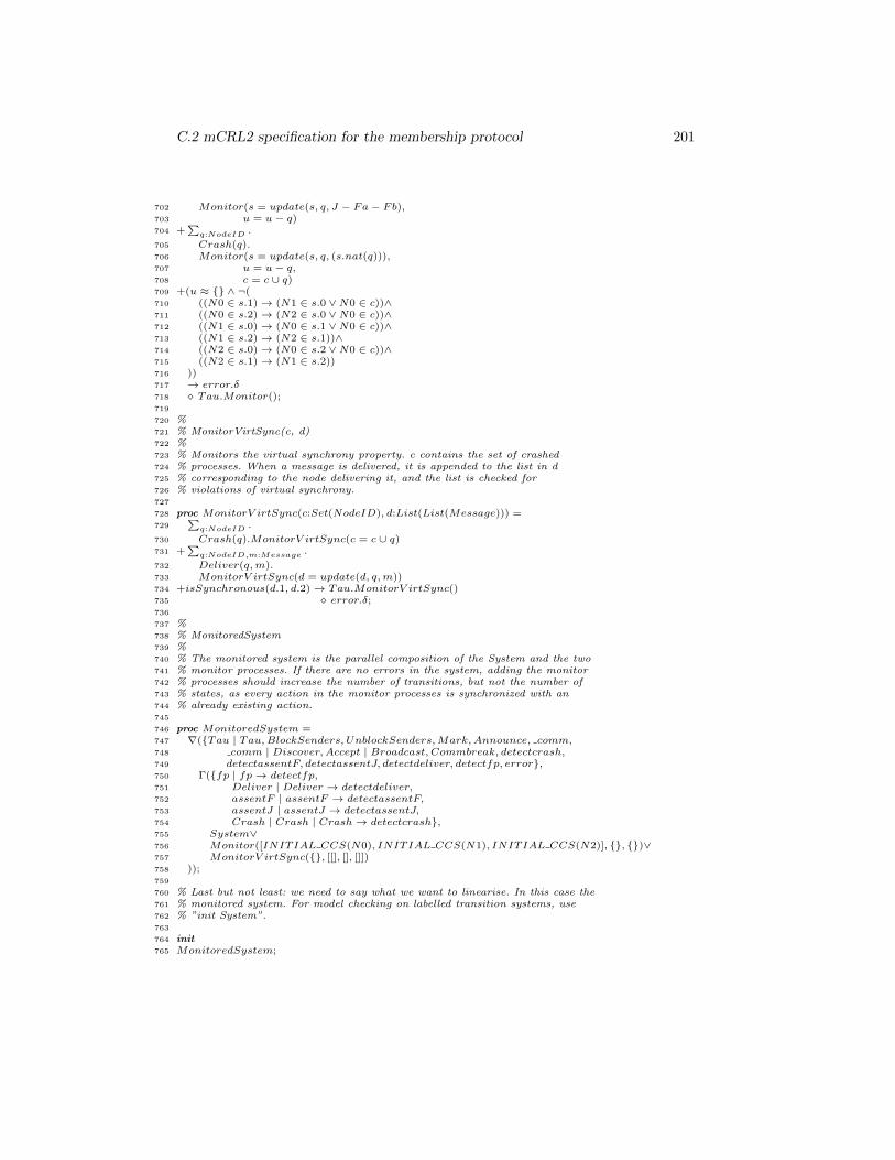
C.2 mCRL2 specification for the membership protocol 201
702 Monitor(s = update(s, q, J − Fa− Fb),703 u = u− q)704 +
∑q:NodeID .
705 Crash(q).706 Monitor(s = update(s, q, (s.nat(q))),707 u = u− q,708 c = c ∪ q)709 +(u ≈ {} ∧ ¬(710 ((N0 ∈ s.1)→ (N1 ∈ s.0 ∨N0 ∈ c))∧711 ((N0 ∈ s.2)→ (N2 ∈ s.0 ∨N0 ∈ c))∧712 ((N1 ∈ s.0)→ (N0 ∈ s.1 ∨N0 ∈ c))∧713 ((N1 ∈ s.2)→ (N2 ∈ s.1))∧714 ((N2 ∈ s.0)→ (N0 ∈ s.2 ∨N0 ∈ c))∧715 ((N2 ∈ s.1)→ (N1 ∈ s.2))716 ))717 → error.δ718 � Tau.Monitor();719
720 %721 % MonitorVirtSync(c, d)722 %723 % Monitors the virtual synchrony property. c contains the set of crashed724 % processes. When a message is delivered, it is appended to the list in d725 % corresponding to the node delivering it, and the list is checked for726 % violations of virtual synchrony.727
728 proc MonitorV irtSync(c:Set(NodeID), d:List(List(Message))) =729
∑q:NodeID .
730 Crash(q).MonitorV irtSync(c = c ∪ q)731 +
∑q:NodeID,m:Message .
732 Deliver(q,m).733 MonitorV irtSync(d = update(d, q,m))734 +isSynchronous(d.1, d.2)→ Tau.MonitorV irtSync()735 � error.δ;736
737 %738 % MonitoredSystem739 %740 % The monitored system is the parallel composition of the System and the two741 % monitor processes. If there are no errors in the system, adding the monitor742 % processes should increase the number of transitions, but not the number of743 % states, as every action in the monitor processes is synchronized with an744 % already existing action.745
746 proc MonitoredSystem =747 ∇({Tau | Tau,BlockSenders, UnblockSenders,Mark,Announce, comm,748 comm | Discover, Accept | Broadcast, Commbreak, detectcrash,749 detectassentF, detectassentJ, detectdeliver, detectfp, error},750 Γ({fp | fp→ detectfp,751 Deliver | Deliver → detectdeliver,752 assentF | assentF → detectassentF,753 assentJ | assentJ → detectassentJ,754 Crash | Crash | Crash→ detectcrash},755 System∨756 Monitor([INITIAL CCS(N0), INITIAL CCS(N1), INITIAL CCS(N2)], {}, {})∨757 MonitorV irtSync({}, [[], [], []])758 ));759
760 % Last but not least: we need to say what we want to linearise. In this case the761 % monitored system. For model checking on labelled transition systems, use762 % ”init System”.763
764 init765 MonitoredSystem;

202 Appendix C. Membership protocols
Appendix D
mCRL2/FDR2Specifications for FailureDetectors
203
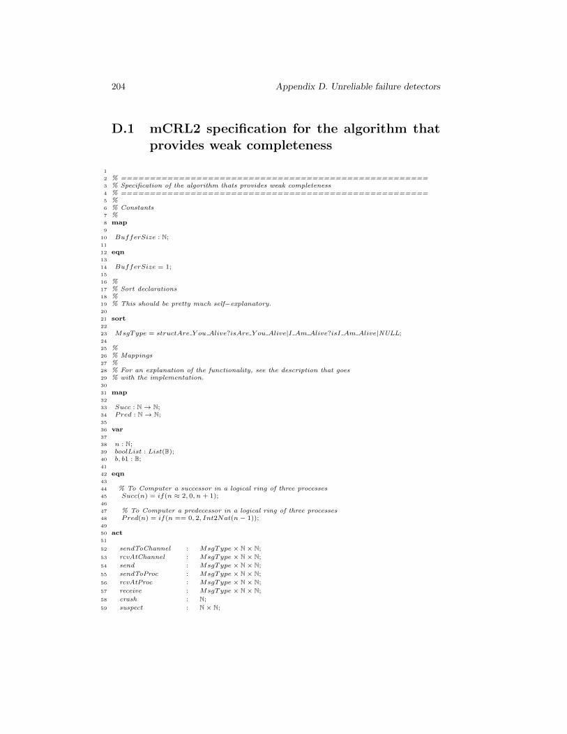
204 Appendix D. Unreliable failure detectors
D.1 mCRL2 specification for the algorithm thatprovides weak completeness
1
2 % =====================================================3 % Specification of the algorithm thats provides weak completeness4 % =====================================================5 %6 % Constants7 %8 map9
10 BufferSize : N;11
12 eqn13
14 BufferSize = 1;15
16 %17 % Sort declarations18 %19 % This should be pretty much self−explanatory.20
21 sort22
23 MsgType = structAre Y ou Alive?isAre Y ou Alive|I Am Alive?isI Am Alive|NULL;24
25 %26 % Mappings27 %28 % For an explanation of the functionality, see the description that goes29 % with the implementation.30
31 map32
33 Succ : N→ N;34 Pred : N→ N;35
36 var37
38 n : N;39 boolList : List(B);40 b, b1 : B;41
42 eqn43
44 % To Computer a successor in a logical ring of three processes45 Succ(n) = if(n ≈ 2, 0, n+ 1);46
47 % To Computer a predecessor in a logical ring of three processes48 Pred(n) = if(n == 0, 2, Int2Nat(n− 1));49
50 act51
52 sendToChannel : MsgType× N× N;
53 rcvAtChannel : MsgType× N× N;
54 send : MsgType× N× N;
55 sendToProc : MsgType× N× N;
56 rcvAtProc : MsgType× N× N;
57 receive : MsgType× N× N;
58 crash : N;
59 suspect : N× N;
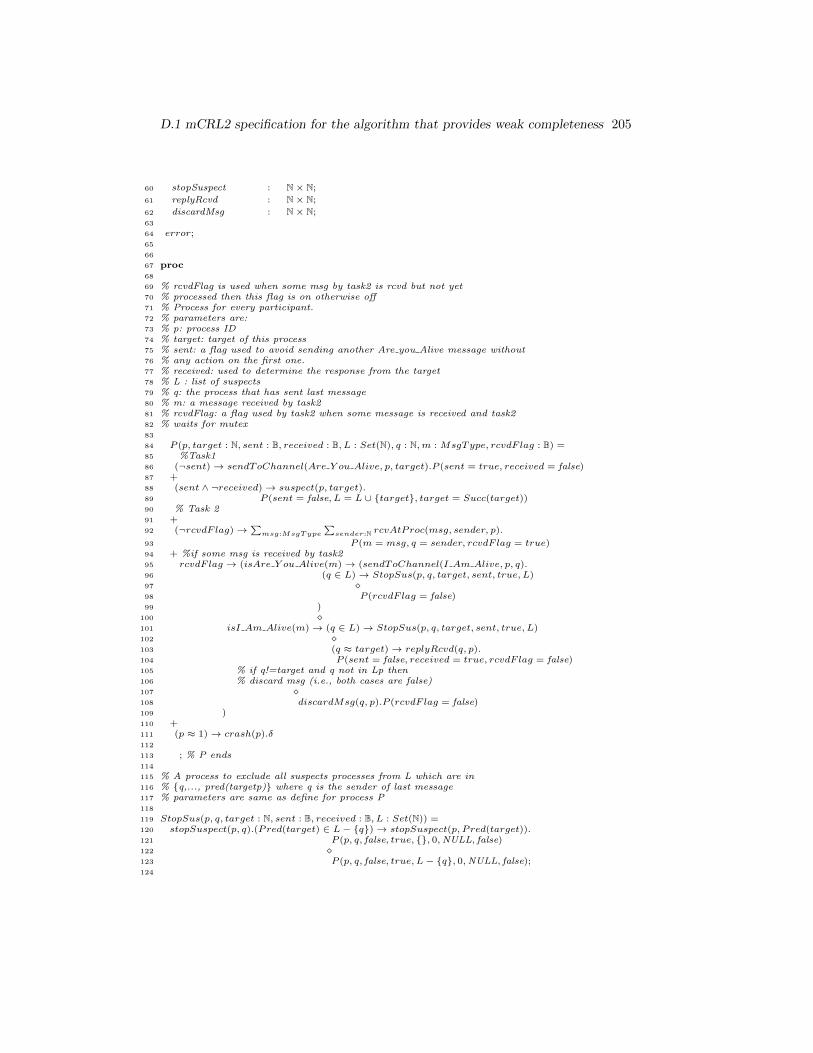
D.1 mCRL2 specification for the algorithm that provides weak completeness 205
60 stopSuspect : N× N;
61 replyRcvd : N× N;
62 discardMsg : N× N;63
64 error;65
66
67 proc68
69 % rcvdFlag is used when some msg by task2 is rcvd but not yet70 % processed then this flag is on otherwise off71 % Process for every participant.72 % parameters are:73 % p: process ID74 % target: target of this process75 % sent: a flag used to avoid sending another Are you Alive message without76 % any action on the first one.77 % received: used to determine the response from the target78 % L : list of suspects79 % q: the process that has sent last message80 % m: a message received by task281 % rcvdFlag: a flag used by task2 when some message is received and task282 % waits for mutex83
84 P (p, target : N, sent : B, received : B, L : Set(N), q : N,m : MsgType, rcvdF lag : B) =85 %Task186 (¬sent)→ sendToChannel(Are Y ou Alive, p, target).P (sent = true, received = false)87 +88 (sent ∧ ¬received)→ suspect(p, target).89 P (sent = false, L = L ∪ {target}, target = Succ(target))90 % Task 291 +92 (¬rcvdF lag)→∑
msg:MsgType
∑sender:N rcvAtProc(msg, sender, p).
93 P (m = msg, q = sender, rcvdF lag = true)94 + %if some msg is received by task295 rcvdF lag → (isAre Y ou Alive(m)→ (sendToChannel(I Am Alive, p, q).96 (q ∈ L)→ StopSus(p, q, target, sent, true, L)97 �98 P (rcvdF lag = false)99 )
100 �101 isI Am Alive(m)→ (q ∈ L)→ StopSus(p, q, target, sent, true, L)102 �103 (q ≈ target)→ replyRcvd(q, p).104 P (sent = false, received = true, rcvdF lag = false)105 % if q!=target and q not in Lp then106 % discard msg (i.e., both cases are false)107 �108 discardMsg(q, p).P (rcvdF lag = false)109 )110 +111 (p ≈ 1)→ crash(p).δ112
113 ; % P ends114
115 % A process to exclude all suspects processes from L which are in116 % {q,..., pred(targetp)} where q is the sender of last message117 % parameters are same as define for process P118
119 StopSus(p, q, target : N, sent : B, received : B, L : Set(N)) =120 stopSuspect(p, q).(Pred(target) ∈ L− {q})→ stopSuspect(p, Pred(target)).121 P (p, q, false, true, {}, 0,NULL, false)122 �123 P (p, q, false, true, L− {q}, 0,NULL, false);124
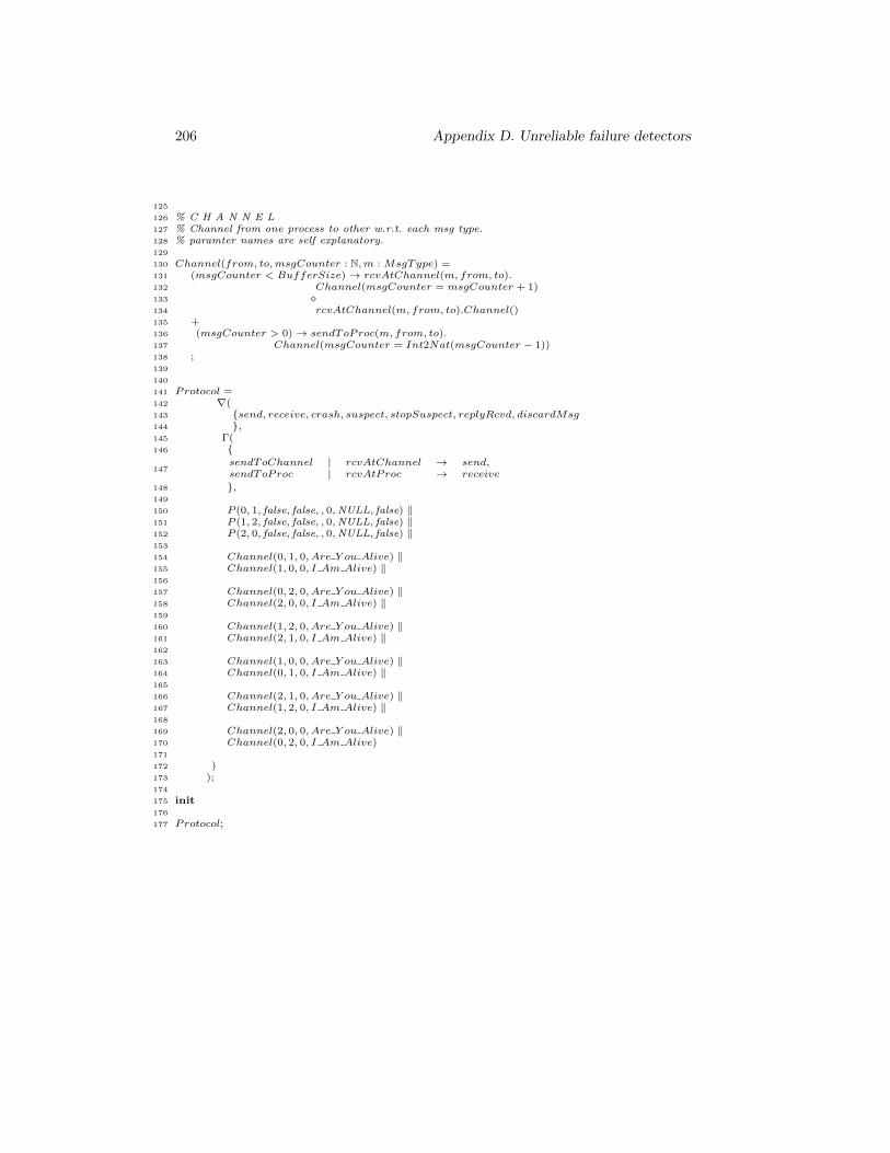
206 Appendix D. Unreliable failure detectors
125
126 % C H A N N E L127 % Channel from one process to other w.r.t. each msg type.128 % paramter names are self explanatory.129
130 Channel(from, to,msgCounter : N,m : MsgType) =131 (msgCounter < BufferSize)→ rcvAtChannel(m, from, to).132 Channel(msgCounter = msgCounter + 1)133 �134 rcvAtChannel(m, from, to).Channel()135 +136 (msgCounter > 0)→ sendToProc(m, from, to).137 Channel(msgCounter = Int2Nat(msgCounter − 1))138 ;139
140
141 Protocol =142 ∇(143 {send, receive, crash, suspect, stopSuspect, replyRcvd, discardMsg144 },145 Γ(146 {147
sendToChannel | rcvAtChannel → send,sendToProc | rcvAtProc → receive
148 },149
150 P (0, 1, false, false, , 0,NULL, false) ‖151 P (1, 2, false, false, , 0,NULL, false) ‖152 P (2, 0, false, false, , 0,NULL, false) ‖153
154 Channel(0, 1, 0, Are Y ou Alive) ‖155 Channel(1, 0, 0, I Am Alive) ‖156
157 Channel(0, 2, 0, Are Y ou Alive) ‖158 Channel(2, 0, 0, I Am Alive) ‖159
160 Channel(1, 2, 0, Are Y ou Alive) ‖161 Channel(2, 1, 0, I Am Alive) ‖162
163 Channel(1, 0, 0, Are Y ou Alive) ‖164 Channel(0, 1, 0, I Am Alive) ‖165
166 Channel(2, 1, 0, Are Y ou Alive) ‖167 Channel(1, 2, 0, I Am Alive) ‖168
169 Channel(2, 0, 0, Are Y ou Alive) ‖170 Channel(0, 2, 0, I Am Alive)171
172 )173 );174
175 init176
177 Protocol;
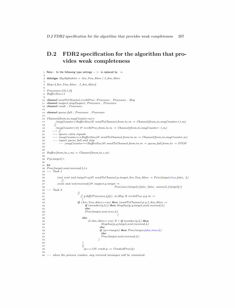
D.2 FDR2 specification for the algorithm that provides weak completeness 207
D.2 FDR2 specification for the algorithm that pro-vides weak completeness
1 Note : In the following type settings − > is replaced by →2
3 datatype MyAlphabets = Are You Alive | I Am Alive4
5 Msg={Are You Alive , I Am Alive}6
7 Processes={0,1,2}8 BufferSize=19
10 channel sendToChannel,rcvAtProc: Processes . Processes . Msg11 channel suspect,stopSuspect: Processes . Processes12 channel crash : Processes13
14 channel queue full : Processes . Processes15
16 Channel(from,to,msgCounter,m)=17 (msgCounter<BufferSize)& sendToChannel.from.to.m → Channel(from,to,msgCounter+1,m)18 []19 (msgCounter>0) & rcvAtProc.from.to.m → Channel(from,to,msgCounter−1,m)20 −− []21 −− ignore extra signals22 −− (msgCounter==BufferSize)& sendToChannel.from.to.m → Channel(from,to,msgCounter,m)23 −− report queue full and stop24 −− (msgCounter==BufferSize)& sendToChannel.from.to.m → queue full.from.to → STOP25
26
27 Buffer(from,to,c,m) = Channel(from,to,c,m)28
29 P(p,target)=30
31 let32 Proc(target,sent,received,L)=33 −− Task 134
35 (not sent and target!=p)& sendToChannel.p.target.Are You Alive → Proc(target,true,false, L)36 []37 (sent and not(received))& suspect.p.target →38 Proc(succ(target),false, false, union(L,{target}))39 −− Task 240 []41 [] q:diff(Processes,{p}), m:Msg @ rcvAtProc.q.p.m →42 (43 if (Are You Alive==m) then (sendToChannel.p.q.I Am Alive →44 if (member(q,L)) then StopSus(p,q,target,sent,received,L)45 else46 Proc(target,sent,true,L)47 )48 else49 (I Am Alive==m) & ( if member(q,L) then50 StopSus(p,q,target,sent,received,L)51 else52 if (q==target) then Proc(target,false,true,L)53 else54 Proc(target,sent,received,L)55 )56 )57 []58 (p==1)& crash.p → CrashedProc(p)59
60 −− when the process crashes, any received messages will be consumed.
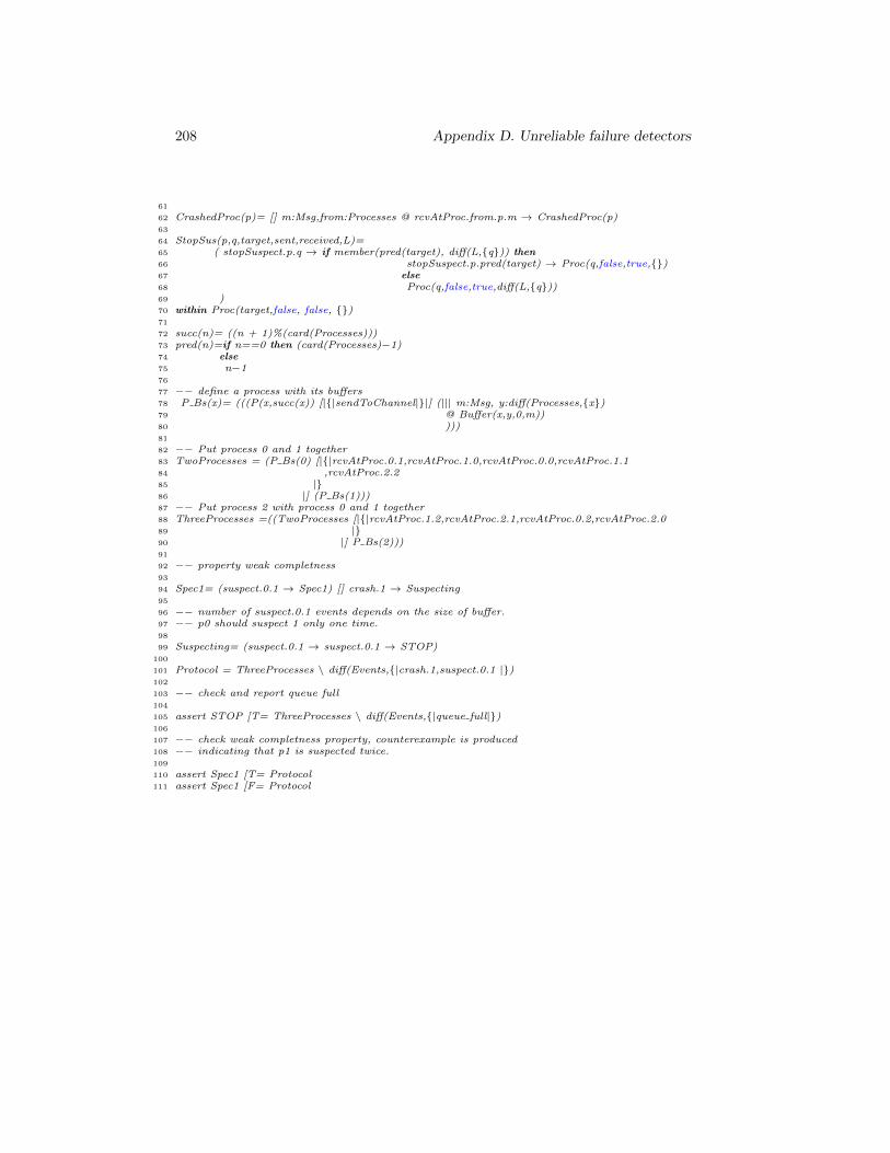
208 Appendix D. Unreliable failure detectors
61
62 CrashedProc(p)= [] m:Msg,from:Processes @ rcvAtProc.from.p.m → CrashedProc(p)63
64 StopSus(p,q,target,sent,received,L)=65 ( stopSuspect.p.q → if member(pred(target), diff(L,{q})) then66 stopSuspect.p.pred(target) → Proc(q,false,true,{})67 else68 Proc(q,false,true,diff(L,{q}))69 )70 within Proc(target,false, false, {})71
72 succ(n)= ((n + 1)%(card(Processes)))73 pred(n)=if n==0 then (card(Processes)−1)74 else75 n−176
77 −− define a process with its buffers78 P Bs(x)= (((P(x,succ(x)) [|{|sendToChannel|}|] (||| m:Msg, y:diff(Processes,{x})79 @ Buffer(x,y,0,m))80 )))81
82 −− Put process 0 and 1 together83 TwoProcesses = (P Bs(0) [|{|rcvAtProc.0.1,rcvAtProc.1.0,rcvAtProc.0.0,rcvAtProc.1.184 ,rcvAtProc.2.285 |}86 |] (P Bs(1)))87 −− Put process 2 with process 0 and 1 together88 ThreeProcesses =((TwoProcesses [|{|rcvAtProc.1.2,rcvAtProc.2.1,rcvAtProc.0.2,rcvAtProc.2.089 |}90 |] P Bs(2)))91
92 −− property weak completness93
94 Spec1= (suspect.0.1 → Spec1) [] crash.1 → Suspecting95
96 −− number of suspect.0.1 events depends on the size of buffer.97 −− p0 should suspect 1 only one time.98
99 Suspecting= (suspect.0.1 → suspect.0.1 → STOP)100
101 Protocol = ThreeProcesses \ diff(Events,{|crash.1,suspect.0.1 |})102
103 −− check and report queue full104
105 assert STOP [T= ThreeProcesses \ diff(Events,{|queue full|})106
107 −− check weak completness property, counterexample is produced108 −− indicating that p1 is suspected twice.109
110 assert Spec1 [T= Protocol111 assert Spec1 [F= Protocol
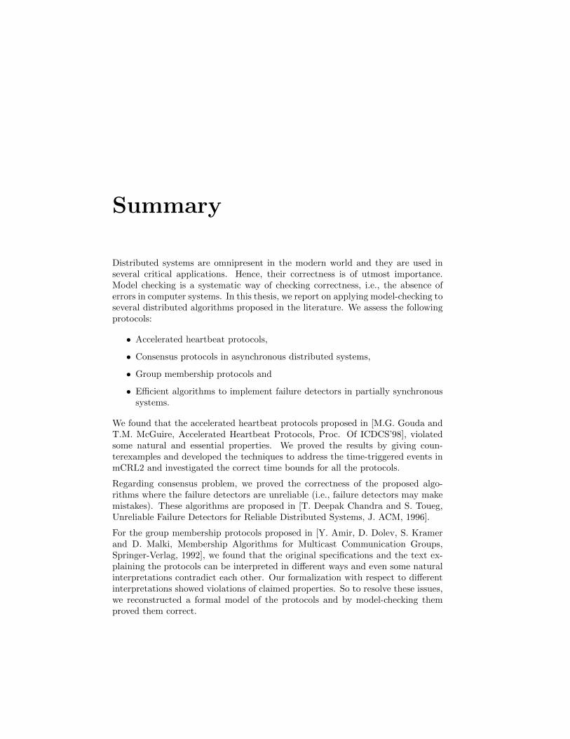
Summary
Distributed systems are omnipresent in the modern world and they are used inseveral critical applications. Hence, their correctness is of utmost importance.Model checking is a systematic way of checking correctness, i.e., the absence oferrors in computer systems. In this thesis, we report on applying model-checking toseveral distributed algorithms proposed in the literature. We assess the followingprotocols:
• Accelerated heartbeat protocols,
• Consensus protocols in asynchronous distributed systems,
• Group membership protocols and
• Efficient algorithms to implement failure detectors in partially synchronoussystems.
We found that the accelerated heartbeat protocols proposed in [M.G. Gouda andT.M. McGuire, Accelerated Heartbeat Protocols, Proc. Of ICDCS’98], violatedsome natural and essential properties. We proved the results by giving coun-terexamples and developed the techniques to address the time-triggered events inmCRL2 and investigated the correct time bounds for all the protocols.
Regarding consensus problem, we proved the correctness of the proposed algo-rithms where the failure detectors are unreliable (i.e., failure detectors may makemistakes). These algorithms are proposed in [T. Deepak Chandra and S. Toueg,Unreliable Failure Detectors for Reliable Distributed Systems, J. ACM, 1996].
For the group membership protocols proposed in [Y. Amir, D. Dolev, S. Kramerand D. Malki, Membership Algorithms for Multicast Communication Groups,Springer-Verlag, 1992], we found that the original specifications and the text ex-plaining the protocols can be interpreted in different ways and even some naturalinterpretations contradict each other. Our formalization with respect to differentinterpretations showed violations of claimed properties. So to resolve these issues,we reconstructed a formal model of the protocols and by model-checking themproved them correct.
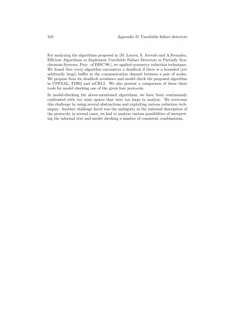
210 Appendix D. Unreliable failure detectors
For analyzing the algorithms proposed in [M. Larrea, S. Arevalo and A.Fernndez,Efficient Algorithms to Implement Unreliable Failure Detectors in Partially Syn-chronous Systems, Proc. of DISC’99 ], we applied symmetry reduction techniques.We found that every algorithm encounters a deadlock if there is a bounded (yetarbitrarily large) buffer in the communication channel between a pair of nodes.We propose fixes for deadlock avoidance and model check the proposed algorithmin UPPAAL, FDR2 and mCRL2. We also present a comparison of these threetools for model checking one of the given four protocols.
In model-checking the above-mentioned algorithms, we have been continuouslyconfronted with too state spaces that were too large to analyze. We overcomethis challenge by using several abstractions and exploiting various reduction tech-niques. Another challenge faced was the ambiguity in the informal description ofthe protocols; in several cases, we had to analyze various possibilities of interpret-ing the informal text and model checking a number of consistent combinations.

Curriculum Vitae
Muhammad Atif was born on the 1st of April 1972 in Samundri, district Faisalabad,Pakistan. In June 1986 he passed the matriculation exam with distinction fromGovernment High School No 1, Samundri and then for secondary education he wentto Mian Channu and passed intermediate examination there in December 1989with pre-engineering subjects. He got his bachelor degree with Mathematics (asmajor) and Physics (as minor) from Bahauddin Zakariya University Multan in May1993. He obtained his master degree in Computer Science from Gomal UniversityD.I.Khan in January 1997. His master project was displayed in All PakistanSoftware Competition and Exhibition 1996 organized by the A.Q. Khan ResearchLaboratories. He has worked with both software companies and universities foralmost eight years. In September 2007 he joined TU/e as Ph.D student on ascholarship issued by the Higher Education Commission of Pakistan.

212 Appendix D. Unreliable failure detectors
Index
µ-calculus, 22
Asynchrony, 5
Causal delivery order, 93Consensus Protocols, 7, 64, 65
Using strong completeness andeventual weak accuracy, 68
Using strong completeness andweak accuracy, 67
Verification results, 86
Efficient algorithms to implement fail-ure detectors in partially syn-chronous systems, 108
Verification results, 120
Failure detectors, 8FDR2, 121
Group membership protocol, 8Group membership protocols, 90
Fault protocol, 95Join protocol, 98Verification results, 101
Heartbeat protocols, 30, 31The binary heartbeat protocol,
31, 32The dynamic heartbeat protocol,
31, 33The expanding heartbeat proto-
col, 31, 33The static heartbeat protocol, 31,
33Verification results, 50
Leader election protocol, 8
mCRL2, 12
Partial synchrony, 4, 109Partially synchronous systems
strong accuracy for failure detec-tors, 112
strong completeness for failure de-tectors, 112
weak accuracy for failure detec-tors, 111
weak completeness for failure de-tectors, 110
Synchrony, 4
Transis, 93
Unreliable failure detector, 64, 108UPPAAL, 24
Virtual Synchrony, 103
213

214 Index
Titles in the IPA Dissertation Series since 2005
E. Abraham. An Assertional ProofSystem for Multithreaded Java -Theoryand Tool Support- . Faculty ofMathematics and Natural Sciences,UL. 2005-01
R. Ruimerman. Modeling andRemodeling in Bone Tissue. Fac-ulty of Biomedical Engineering,TU/e. 2005-02
C.N. Chong. Experiments in RightsControl - Expression and Enforce-ment. Faculty of Electrical Engineer-ing, Mathematics & Computer Science,UT. 2005-03
H. Gao. Design and Verification ofLock-free Parallel Algorithms. Facultyof Mathematics and Computing Sci-ences, RUG. 2005-04
H.M.A. van Beek. Specification andAnalysis of Internet Applications. Fac-ulty of Mathematics and ComputerScience, TU/e. 2005-05
M.T. Ionita. Scenario-Based Sys-tem Architecting - A Systematic Ap-proach to Developing Future-ProofSystem Architectures. Faculty ofMathematics and Computing Sciences,TU/e. 2005-06
G. Lenzini. Integration of Analy-sis Techniques in Security and Fault-Tolerance. Faculty of Electrical En-gineering, Mathematics & ComputerScience, UT. 2005-07
I. Kurtev. Adaptability of ModelTransformations. Faculty of Electri-
cal Engineering, Mathematics & Com-puter Science, UT. 2005-08
T. Wolle. Computational Aspects ofTreewidth - Lower Bounds and Net-work Reliability. Faculty of Science,UU. 2005-09
O. Tveretina. Decision Proceduresfor Equality Logic with UninterpretedFunctions. Faculty of Mathematicsand Computer Science, TU/e. 2005-10
A.M.L. Liekens. Evolution of Fi-nite Populations in Dynamic Environ-ments. Faculty of Biomedical Engi-neering, TU/e. 2005-11
J. Eggermont. Data Mining us-ing Genetic Programming: Classifica-tion and Symbolic Regression. Facultyof Mathematics and Natural Sciences,UL. 2005-12
B.J. Heeren. Top Quality Type Er-ror Messages. Faculty of Science,UU. 2005-13
G.F. Frehse. Compositional Verifi-cation of Hybrid Systems using Sim-ulation Relations. Faculty of Science,Mathematics and Computer Science,RU. 2005-14
M.R. Mousavi. Structuring Struc-tural Operational Semantics. Facultyof Mathematics and Computer Sci-ence, TU/e. 2005-15
A. Sokolova. Coalgebraic Analysisof Probabilistic Systems. Faculty ofMathematics and Computer Science,TU/e. 2005-16
T. Gelsema. Effective Models for theStructure of pi-Calculus Processes withReplication. Faculty of Mathematicsand Natural Sciences, UL. 2005-17
P. Zoeteweij. Composing ConstraintSolvers. Faculty of Natural Sciences,Mathematics, and Computer Science,UvA. 2005-18
J.J. Vinju. Analysis and Transfor-mation of Source Code by Parsing andRewriting. Faculty of Natural Sci-ences, Mathematics, and ComputerScience, UvA. 2005-19
M.Valero Espada. Modal Abstrac-tion and Replication of Processes withData. Faculty of Sciences, Division ofMathematics and Computer Science,VUA. 2005-20
A. Dijkstra. Stepping throughHaskell. Faculty of Science,UU. 2005-21
Y.W. Law. Key management andlink-layer security of wireless sensornetworks: energy-efficient attack anddefense. Faculty of Electrical En-gineering, Mathematics & ComputerScience, UT. 2005-22
E. Dolstra. The Purely FunctionalSoftware Deployment Model. Facultyof Science, UU. 2006-01
R.J. Corin. Analysis Models for Se-curity Protocols. Faculty of Electri-cal Engineering, Mathematics & Com-puter Science, UT. 2006-02
P.R.A. Verbaan. The Computa-tional Complexity of Evolving Systems.Faculty of Science, UU. 2006-03
K.L. Man and R.R.H. Schiffel-ers. Formal Specification and Anal-ysis of Hybrid Systems. Faculty ofMathematics and Computer Scienceand Faculty of Mechanical Engineer-ing, TU/e. 2006-04
M. Kyas. Verifying OCL Specifi-cations of UML Models: Tool Sup-port and Compositionality. Facultyof Mathematics and Natural Sciences,UL. 2006-05
M. Hendriks. Model Checking TimedAutomata - Techniques and Applica-tions. Faculty of Science, Mathematicsand Computer Science, RU. 2006-06
J. Ketema. Bohm-Like Trees forRewriting. Faculty of Sciences,VUA. 2006-07
C.-B. Breunesse. On JML: topics intool-assisted verification of JML pro-grams. Faculty of Science, Mathemat-ics and Computer Science, RU. 2006-08
B. Markvoort. Towards Hy-brid Molecular Simulations. Fac-ulty of Biomedical Engineering,TU/e. 2006-09
S.G.R. Nijssen. Mining StructuredData. Faculty of Mathematics andNatural Sciences, UL. 2006-10
G. Russello. Separation and Adap-tation of Concerns in a Shared DataSpace. Faculty of Mathematics andComputer Science, TU/e. 2006-11
L. Cheung. Reconciling Nonde-terministic and Probabilistic Choices.Faculty of Science, Mathematics andComputer Science, RU. 2006-12
B. Badban. Verification tech-niques for Extensions of EqualityLogic. Faculty of Sciences, Division ofMathematics and Computer Science,VUA. 2006-13
A.J. Mooij. Constructive formalmethods and protocol standardization.Faculty of Mathematics and ComputerScience, TU/e. 2006-14
T. Krilavicius. Hybrid Techniquesfor Hybrid Systems. Faculty of Electri-cal Engineering, Mathematics & Com-puter Science, UT. 2006-15
M.E. Warnier. Language Based Se-curity for Java and JML. Faculty ofScience, Mathematics and ComputerScience, RU. 2006-16
V. Sundramoorthy. At Home InService Discovery. Faculty of Electri-cal Engineering, Mathematics & Com-puter Science, UT. 2006-17
B. Gebremichael. Expressivity ofTimed Automata Models. Faculty ofScience, Mathematics and ComputerScience, RU. 2006-18
L.C.M. van Gool. FormalisingInterface Specifications. Faculty ofMathematics and Computer Science,TU/e. 2006-19
C.J.F. Cremers. Scyther - Seman-tics and Verification of Security Pro-tocols. Faculty of Mathematics andComputer Science, TU/e. 2006-20
J.V. Guillen Scholten. MobileChannels for Exogenous Coordina-tion of Distributed Systems: Seman-tics, Implementation and Composition.
Faculty of Mathematics and NaturalSciences, UL. 2006-21
H.A. de Jong. Flexible Heteroge-neous Software Systems. Faculty ofNatural Sciences, Mathematics, andComputer Science, UvA. 2007-01
N.K. Kavaldjiev. A run-time recon-figurable Network-on-Chip for stream-ing DSP applications. Faculty ofElectrical Engineering, Mathematics &Computer Science, UT. 2007-02
M. van Veelen. Considerationson Modeling for Early Detection ofAbnormalities in Locally AutonomousDistributed Systems. Faculty ofMathematics and Computing Sciences,RUG. 2007-03
T.D. Vu. Semantics and Applicationsof Process and Program Algebra. Fac-ulty of Natural Sciences, Mathematics,and Computer Science, UvA. 2007-04
L. Brandan Briones. Theories forModel-based Testing: Real-time andCoverage. Faculty of Electrical En-gineering, Mathematics & ComputerScience, UT. 2007-05
I. Loeb. Natural Deduction: Shar-ing by Presentation. Faculty of Sci-ence, Mathematics and Computer Sci-ence, RU. 2007-06
M.W.A. Streppel. MultifunctionalGeometric Data Structures. Faculty ofMathematics and Computer Science,TU/e. 2007-07
N. Trcka. Silent Steps in Transi-tion Systems and Markov Chains. Fac-ulty of Mathematics and ComputerScience, TU/e. 2007-08
R. Brinkman. Searching in en-crypted data. Faculty of Electrical En-gineering, Mathematics & ComputerScience, UT. 2007-09
A. van Weelden. Putting typesto good use. Faculty of Science,Mathematics and Computer Science,RU. 2007-10
J.A.R. Noppen. Imperfect Infor-mation in Software Development Pro-cesses. Faculty of Electrical Engineer-ing, Mathematics & Computer Science,UT. 2007-11
R. Boumen. Integration and Testplans for Complex Manufacturing Sys-tems. Faculty of Mechanical Engineer-ing, TU/e. 2007-12
A.J. Wijs. What to do Next?:Analysing and Optimising System Be-haviour in Time. Faculty of Sciences,Division of Mathematics and Com-puter Science, VUA. 2007-13
C.F.J. Lange. Assessing and Improv-ing the Quality of Modeling: A Seriesof Empirical Studies about the UML.Faculty of Mathematics and ComputerScience, TU/e. 2007-14
T. van der Storm. Component-based Configuration, Integration andDelivery. Faculty of Natural Sci-ences, Mathematics, and ComputerScience,UvA. 2007-15
B.S. Graaf. Model-Driven Evolutionof Software Architectures. Faculty ofElectrical Engineering, Mathematics,and Computer Science, TUD. 2007-16
A.H.J. Mathijssen. Logical Calculifor Reasoning with Binding. Faculty of
Mathematics and Computer Science,TU/e. 2007-17
D. Jarnikov. QoS framework forVideo Streaming in Home Networks.Faculty of Mathematics and ComputerScience, TU/e. 2007-18
M. A. Abam. New Data Structuresand Algorithms for Mobile Data. Fac-ulty of Mathematics and ComputerScience, TU/e. 2007-19
W. Pieters. La Volonte Machi-nale: Understanding the ElectronicVoting Controversy. Faculty of Sci-ence, Mathematics and Computer Sci-ence, RU. 2008-01
A.L. de Groot. Practical Automa-ton Proofs in PVS. Faculty of Science,Mathematics and Computer Science,RU. 2008-02
M. Bruntink. Renovation of Id-iomatic Crosscutting Concerns in Em-bedded Systems. Faculty of ElectricalEngineering, Mathematics, and Com-puter Science, TUD. 2008-03
A.M. Marin. An Integrated Sys-tem to Manage Crosscutting Concernsin Source Code. Faculty of ElectricalEngineering, Mathematics, and Com-puter Science, TUD. 2008-04
N.C.W.M. Braspenning. Model-based Integration and Testing ofHigh-tech Multi-disciplinary Systems.Faculty of Mechanical Engineering,TU/e. 2008-05
M. Bravenboer. Exercises in FreeSyntax: Syntax Definition, Pars-ing, and Assimilation of Language
Conglomerates. Faculty of Science,UU. 2008-06
M. Torabi Dashti. Keeping Fair-ness Alive: Design and Formal Ver-ification of Optimistic Fair ExchangeProtocols. Faculty of Sciences, Di-vision of Mathematics and ComputerScience, VUA. 2008-07
I.S.M. de Jong. Integration and TestStrategies for Complex ManufacturingMachines. Faculty of Mechanical En-gineering, TU/e. 2008-08
I. Hasuo. Tracing Anonymity withCoalgebras. Faculty of Science,Mathematics and Computer Science,RU. 2008-09
L.G.W.A. Cleophas. Tree Al-gorithms: Two Taxonomies and aToolkit. Faculty of Mathematics andComputer Science, TU/e. 2008-10
I.S. Zapreev. Model CheckingMarkov Chains: Techniques and Tools.Faculty of Electrical Engineering,Mathematics & Computer Science,UT. 2008-11
M. Farshi. A Theoretical and Exper-imental Study of Geometric Networks.Faculty of Mathematics and ComputerScience, TU/e. 2008-12
G. Gulesir. Evolvable BehaviorSpecifications Using Context-SensitiveWildcards. Faculty of Electrical En-gineering, Mathematics & ComputerScience, UT. 2008-13
F.D. Garcia. Formal and Com-putational Cryptography: Protocols,Hashes and Commitments. Faculty of
Science, Mathematics and ComputerScience, RU. 2008-14
P. E. A. Durr. Resource-based Veri-fication for Robust Composition of As-pects. Faculty of Electrical Engineer-ing, Mathematics & Computer Science,UT. 2008-15
E.M. Bortnik. Formal Meth-ods in Support of SMC Design.Faculty of Mechanical Engineering,TU/e. 2008-16
R.H. Mak. Design and Perfor-mance Analysis of Data-IndependentStream Processing Systems. Faculty ofMathematics and Computer Science,TU/e. 2008-17
M. van der Horst. Scalable BlockProcessing Algorithms. Faculty ofMathematics and Computer Science,TU/e. 2008-18
C.M. Gray. Algorithms for Fat Ob-jects: Decompositions and Applica-tions. Faculty of Mathematics andComputer Science, TU/e. 2008-19
J.R. Calame. Testing Reactive Sys-tems with Data - Enumerative Meth-ods and Constraint Solving. Faculty ofElectrical Engineering, Mathematics &Computer Science, UT. 2008-20
E. Mumford. Drawing Graphs forCartographic Applications. Faculty ofMathematics and Computer Science,TU/e. 2008-21
E.H. de Graaf. Mining Semi-structured Data, Theoretical and Ex-perimental Aspects of Pattern Evalua-tion. Faculty of Mathematics and Nat-ural Sciences, UL. 2008-22
R. Brijder. Models of Natural Com-putation: Gene Assembly and Mem-brane Systems. Faculty of Mathemat-ics and Natural Sciences, UL. 2008-23
A. Koprowski. Termination ofRewriting and Its Certification. Fac-ulty of Mathematics and ComputerScience, TU/e. 2008-24
U. Khadim. Process Algebras for Hy-brid Systems: Comparison and Devel-opment. Faculty of Mathematics andComputer Science, TU/e. 2008-25
J. Markovski. Real and Stochas-tic Time in Process Algebras for Per-formance Evaluation. Faculty ofMathematics and Computer Science,TU/e. 2008-26
H. Kastenberg. Graph-Based Soft-ware Specification and Verification.Faculty of Electrical Engineering,Mathematics & Computer Science,UT. 2008-27
I.R. Buhan. Cryptographic Keysfrom Noisy Data Theory and Applica-tions. Faculty of Electrical Engineer-ing, Mathematics & Computer Science,UT. 2008-28
R.S. Marin-Perianu. Wireless Sen-sor Networks in Motion: ClusteringAlgorithms for Service Discovery andProvisioning. Faculty of Electrical En-gineering, Mathematics & ComputerScience, UT. 2008-29
M.H.G. Verhoef. Modeling andValidating Distributed Embedded Real-Time Control Systems. Faculty of Sci-ence, Mathematics and Computer Sci-ence, RU. 2009-01
M. de Mol. Reasoning about Func-tional Programs: Sparkle, a proof as-sistant for Clean. Faculty of Science,Mathematics and Computer Science,RU. 2009-02
M. Lormans. Managing Require-ments Evolution. Faculty of ElectricalEngineering, Mathematics, and Com-puter Science, TUD. 2009-03
M.P.W.J. van Osch. AutomatedModel-based Testing of Hybrid Sys-tems. Faculty of Mathematics andComputer Science, TU/e. 2009-04
H. Sozer. Architecting Fault-TolerantSoftware Systems. Faculty of Electri-cal Engineering, Mathematics & Com-puter Science, UT. 2009-05
M.J. van Weerdenburg. EfficientRewriting Techniques. Faculty ofMathematics and Computer Science,TU/e. 2009-06
H.H. Hansen. Coalgebraic Mod-elling: Applications in Automata The-ory and Modal Logic. Faculty of Sci-ences, Division of Mathematics andComputer Science, VUA. 2009-07
A. Mesbah. Analysis and Testingof Ajax-based Single-page Web Appli-cations. Faculty of Electrical Engineer-ing, Mathematics, and Computer Sci-ence, TUD. 2009-08
A.L. Rodriguez Yakushev. To-wards Getting Generic ProgrammingReady for Prime Time. Faculty of Sci-ence, UU. 2009-9
K.R. Olmos Joffre. Strategies forContext Sensitive Program Trans-
formation. Faculty of Science,UU. 2009-10
J.A.G.M. van den Berg. Reason-ing about Java programs in PVS usingJML. Faculty of Science, Mathematicsand Computer Science, RU. 2009-11
M.G. Khatib. MEMS-Based Stor-age Devices. Integration in Energy-Constrained Mobile Systems. Facultyof Electrical Engineering, Mathematics& Computer Science, UT. 2009-12
S.G.M. Cornelissen. Evaluating Dy-namic Analysis Techniques for Pro-gram Comprehension. Faculty of Elec-trical Engineering, Mathematics, andComputer Science, TUD. 2009-13
D. Bolzoni. Revisiting Anomaly-based Network Intrusion DetectionSystems. Faculty of Electrical En-gineering, Mathematics & ComputerScience, UT. 2009-14
H.L. Jonker. Security Matters: Pri-vacy in Voting and Fairness in DigitalExchange. Faculty of Mathematics andComputer Science, TU/e. 2009-15
M.R. Czenko. TuLiP - ReshapingTrust Management. Faculty of Electri-cal Engineering, Mathematics & Com-puter Science, UT. 2009-16
T. Chen. Clocks, Dice and Pro-cesses. Faculty of Sciences, Division ofMathematics and Computer Science,VUA. 2009-17
C. Kaliszyk. Correctness and Avail-ability: Building Computer Algebraon top of Proof Assistants and mak-ing Proof Assistants available over the
Web. Faculty of Science, Mathematicsand Computer Science, RU. 2009-18
R.S.S. O’Connor. Incompleteness &Completeness: Formalizing Logic andAnalysis in Type Theory. Faculty ofScience, Mathematics and ComputerScience, RU. 2009-19
B. Ploeger. Improved VerificationMethods for Concurrent Systems. Fac-ulty of Mathematics and ComputerScience, TU/e. 2009-20
T. Han. Diagnosis, Synthesisand Analysis of Probabilistic Mod-els. Faculty of Electrical Engineer-ing, Mathematics & Computer Science,UT. 2009-21
R. Li. Mixed-Integer Evolution Strate-gies for Parameter Optimization andTheir Applications to Medical ImageAnalysis. Faculty of Mathematics andNatural Sciences, UL. 2009-22
J.H.P. Kwisthout. The Computa-tional Complexity of Probabilistic Net-works. Faculty of Science, UU. 2009-23
T.K. Cocx. Algorithmic Tools forData-Oriented Law Enforcement. Fac-ulty of Mathematics and Natural Sci-ences, UL. 2009-24
A.I. Baars. Embedded Compilers.Faculty of Science, UU. 2009-25
M.A.C. Dekker. Flexible AccessControl for Dynamic Collaborative En-vironments. Faculty of Electrical En-gineering, Mathematics & ComputerScience, UT. 2009-26
J.F.J. Laros. Metrics and Visualisa-tion for Crime Analysis and Genomics.
Faculty of Mathematics and NaturalSciences, UL. 2009-27
C.J. Boogerd. Focusing AutomaticCode Inspections. Faculty of ElectricalEngineering, Mathematics, and Com-puter Science, TUD. 2010-01
M.R. Neuhaußer. Model Check-ing Nondeterministic and RandomlyTimed Systems. Faculty of Electri-cal Engineering, Mathematics & Com-puter Science, UT. 2010-02
J. Endrullis. Termination and Pro-ductivity. Faculty of Sciences, Divi-sion of Mathematics and ComputerScience, VUA. 2010-03
T. Staijen. Graph-Based Specificationand Verification for Aspect-OrientedLanguages. Faculty of Electrical En-gineering, Mathematics & ComputerScience, UT. 2010-04
Y. Wang. Epistemic Modelling andProtocol Dynamics. Faculty of Science,UvA. 2010-05
J.K. Berendsen. Abstraction, Pricesand Probability in Model CheckingTimed Automata. Faculty of Science,Mathematics and Computer Science,RU. 2010-06
A. Nugroho. The Effects of UMLModeling on the Quality of Software.Faculty of Mathematics and NaturalSciences, UL. 2010-07
A. Silva. Kleene Coalgebra. Fac-ulty of Science, Mathematics and Com-puter Science, RU. 2010-08
J.S. de Bruin. Service-Oriented
Discovery of Knowledge - Founda-tions, Implementations and Applica-tions. Faculty of Mathematics andNatural Sciences, UL. 2010-09
D. Costa. Formal Models for Com-ponent Connectors. Faculty of Sci-ences, Division of Mathematics andComputer Science, VUA. 2010-10
M.M. Jaghoori. Time at Your Ser-vice: Schedulability Analysis of Real-Time and Distributed Services. Fac-ulty of Mathematics and Natural Sci-ences, UL. 2010-11
R. Bakhshi. Gossiping Models: For-mal Analysis of Epidemic Protocols.Faculty of Sciences, Department ofComputer Science, VUA. 2011-01
B.J. Arnoldus. An Illumination ofthe Template Enigma: Software CodeGeneration with Templates. Faculty ofMathematics and Computer Science,TU/e. 2011-02
E. Zambon. Towards Optimal ITAvailability Planning: Methods andTools. Faculty of Electrical Engineer-ing, Mathematics & Computer Science,UT. 2011-03
L. Astefanoaei. An Executable The-ory of Multi-Agent Systems Refine-ment. Faculty of Mathematics andNatural Sciences, UL. 2011-04
J. Proenca. Synchronous coordina-tion of distributed components. Fac-ulty of Mathematics and Natural Sci-ences, UL. 2011-05
A. Moralı. IT Architecture-BasedConfidentiality Risk Assessment inNetworks of Organizations. Faculty of
Electrical Engineering, Mathematics &Computer Science, UT. 2011-06
M. van der Bijl. On changing mod-els in Model-Based Testing. Faculty ofElectrical Engineering, Mathematics &Computer Science, UT. 2011-07
C. Krause. Reconfigurable Com-ponent Connectors. Faculty ofMathematics and Natural Sciences,UL. 2011-08
M.E. Andres. Quantitative Analy-sis of Information Leakage in Proba-bilistic and Nondeterministic Systems.Faculty of Science, Mathematics andComputer Science, RU. 2011-09
M. Atif. Formal Modeling and Verifi-cation of Distributed Failure Detectors.Faculty of Mathematics and ComputerScience, TU/e. 2011-10